SVDD-Based Pattern Denoising

LETTER Communicated by Klaus-Robert Muller

SVDD-Based Pattern Denoising

Jooyoung [email protected] [email protected] of Control and Instrumentation Engineering, Korea University,Jochiwon, Chungnam, 339-700, Korea

Jongho [email protected] and Manufacturing Technology Center, Samsung Electronics Co., Ltd.,Suwon, Gyeonggi, 443-742, Korea

James T. [email protected] W. [email protected] of Computer Science and Engineering, Hong Kong University of Scienceand Technology, Clear Water Bay, Hong Kong

The support vector data description (SVDD) is one of the best-knownone-class support vector learning methods, in which one tries the strategyof using balls defined on the feature space in order to distinguish aset of normal data from all other possible abnormal objects. The majorconcern of this letter is to extend the main idea of SVDD to patterndenoising. Combining the geodesic projection to the spherical decisionboundary resulting from the SVDD, together with solving the preimageproblem, we propose a new method for pattern denoising. We first solveSVDD for the training data and then for each noisy test pattern, obtain itsdenoised feature by moving its feature vector along the geodesic on themanifold to the nearest decision boundary of the SVDD ball. Finally wefind the location of the denoised pattern by obtaining the pre-image of thedenoised feature. The applicability of the proposed method is illustratedby a number of toy and real-world data sets.

1 Introduction

Recently, the support vector learning method has become a viable tool inthe area of intelligent systems (Cristianini & Shawe-Taylor, 2000; Scholkopf& Smola, 2002). Among the important application areas for support

Neural Computation 19, 1919–1938 (2007) C© 2007 Massachusetts Institute of Technology

1920 J. Park et al.

vector learning, we have the one-class classification problems (Campbell &Bennett, 2001; Crammer & Chechik, 2004; Lanckriet, El Ghaoui, & Jordan,2003; Laskov, Schafer, & Kotenko, 2004; Muller, Mika, Ratsch, Tsuda, &Scholkopf, 2001; Pekalska, Tax, & Duin, 2003; Ratsch, Mika, Scholkopf,& Muller, 2002; Scholkopf, Platt, & Smola, 2000; Scholkopf, Platt, Shawe-Taylor, Smola, & Williamson, 2001; Scholkopf & Smola, 2002; Tax, 2001;Tax & Duin, 1999). In one-class classification problems, we are givenonly the training data for the normal class, and after the training phaseis finished, we are required to decide whether each test vector belongsto the normal or the abnormal class. One-class classification problemsare often called outlier detection problems or novelty detection prob-lems. Obvious examples of this class include fault detection for machinesand the intrusion detection system for computers (Scholkopf & Smola,2002).

One of the best-known support vector learning methods for the one-class problems is the SVDD (support vector data description) (Tax, 2001;Tax & Duin, 1999). In the SVDD, balls are used for expressing the regionfor the normal class. Among the methods having the same purpose withthe SVDD are the so-called one-class SVM of Scholkopf and others (Ratschet al., 2002; Scholkopf et al., 2001; Scholkopf et al., 2000), the linear program-ming method of Campbell and Bennet (2001), the information-bottleneck-principle-based optimization approach of Crammer and Chechik (2004),and the single-class minimax probability machine of Lanckriet et al.(2003). Since balls on the input domain can express only a limitedclass of regions, the SVDD in general enhances its expressing powerby utilizing balls on the feature space instead of the balls on the inputdomain.

In this letter, we extend the main idea of the SVDD toward the use forthe problem of pattern denoising (Kwok & Tsang, 2004; Mika et al., 1999;Scholkopf et al., 1999). Combining the movement to the spherical decisionboundary resulting from the SVDD together with a solver for the preimageproblem, we propose a new method for pattern denoising that consists ofthe following steps. First, we solve the SVDD for the training data consistingof the prototype patterns. Second, for each noisy test pattern, we obtain itsdenoised feature by moving its feature vector along the geodesic to thespherical decision boundary of the SVDD ball on the feature space. Finallyin the third step, we recover the location of the denoised pattern by obtainingthe preimage of the denoised feature following the strategy of Kwok andTsang (2004).

The remaining parts of this letter are organized as follows. In section 2,preliminaries are provided regarding the SVDD. Our main results on pat-tern denoising based on the SVDD are presented in section 3. In section4, the applicability of the proposed method is illustrated by a number oftoy and real-world data sets. Finally, in section 5, concluding remarks aregiven.

SVDD-Based Pattern Denoising 1921

2 Preliminaries

The SVDD method, which approximates the support of objects belonging tonormal class, is derived as follows (Tax, 2001; Tax & Duin, 1999). Consider aball B with center a ∈ R

d and radius R, and the training data set D consistingof objects xi ∈ R

d , i = 1, . . . , N. The main idea of SVDD is to find a ball thatcan achieve two conflicting goals (it should be as small as possible andcontain as many training data as possible) simultaneously by solving

min L0(R2, a, ξ ) = R2 + CN∑

i=1

ξi

s.t. ‖xi − a‖2 ≤ R2 + ξi , ξi ≥ 0, i = 1, . . . , N. (2.1)

Here, the slack variable ξi represents the penalty associated with the devia-tion of the ith training pattern outside the ball, and C is a trade-off constantcontrolling the relative importance of each term. The dual problem of equa-tion 2.1 is

maxα

N∑i=1

αi 〈xi , xi 〉 −N∑

i=1

N∑j=1

αi α j 〈xi , x j 〉

s.t.N∑

i=1

αi = 1, αi ∈ [0, C], i = 1, . . . , N. (2.2)

In order to express more complex decision regions in Rd , one can use the

so-called feature map φ : Rd → F and balls defined on the feature space F .

Proceeding similar to the above and utilizing the kernel trick 〈φ(x), φ(z)〉 =k(x, z), one can find the corresponding feature space SVDD ball BF in F .Moreover, from the Kuhn-Tucker condition, its center can be expressed as

aF =N∑

i=1

αiφ(xi ), (2.3)

and its radius RF can be computed by utilizing the distance between aF

and any support vector x on the ball boundary:

R2F = k(x, x) − 2

N∑i=1

αi k(xi , x) +N∑

i=1

N∑j=1

αiα j k(xi , x j ). (2.4)

In this letter, we always use the gaussian kernel k(x, z) = exp(−‖x − z‖2/s2),and so k(x, x) = 1 for each x ∈ R

d . Finally, note that in this case, the SVDD

1922 J. Park et al.

formulation is equivalent to

minα

N∑i=1

N∑j=1

αiα j k(xi , x j )

s.t.N∑

i=1

αi = 1, αi ∈ [0, C], i = 1, . . . , N, (2.5)

and the resulting criterion for the normality is

fF (x)= R2

F − ‖φ(x) − aF ‖2 ≥ 0. (2.6)

3 Main Results

In SVDD, the objective is to find the support of the normal objects; anythingoutside the support is viewed as abnormal. In the feature space, the supportis expressed by a reasonably small ball containing a reasonably large portionof the φ(xi )’s. The main idea of this letter is to utilize the ball-shaped supporton the feature space for correcting test inputs distorted by noise. Moreprecisely, with the trade-off constant C set appropriately,1 we can find aregion where the normal objects without noise generally reside. When anobject (which was originally normal) is given as a test input x in a distortedform, the network resulting from the SVDD is supposed to judge that thedistorted object x does not belong to the normal class. The role of the SVDDhas been conventional up to this point, and the problem of curing thedistortion might be thought of as beyond the scope of the SVDD.

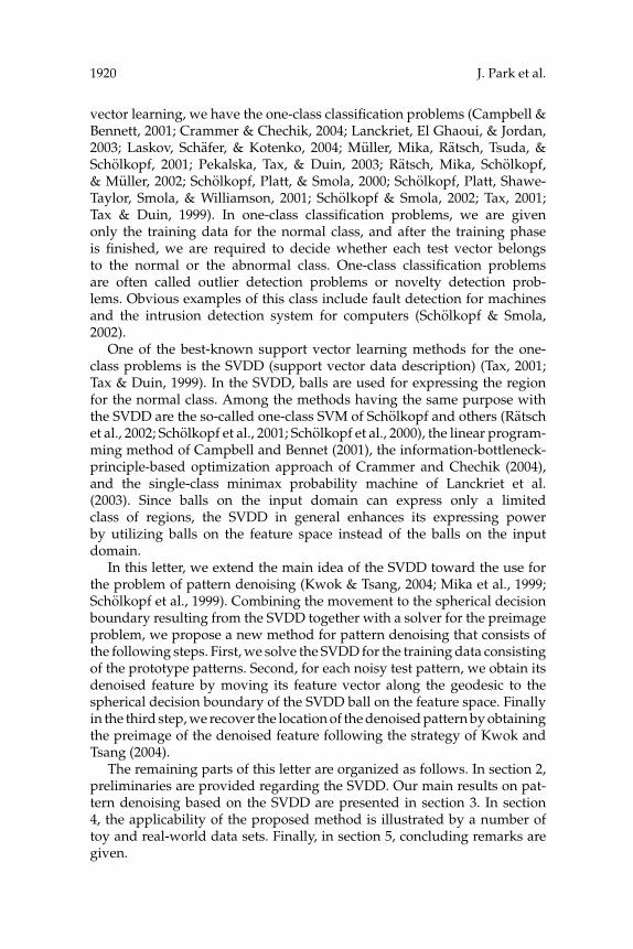
In this letter, we go one step further and move the feature vector φ(x)of the distorted test input x to the point Qφ(x) lying on the surface of theSVDD ball BF so that it can be tailored enough to be normal (see Figure 1).Given that all the points in the input space are mapped to a manifold inthe kernel-induced feature space (Burges, 1999), the movement is alongthe geodesic on this manifold, and so the point Qφ(x) can be consideredas the geodesic projection of φ(x) onto the SVDD ball. Of course, sincethe movement starts from the distorted feature φ(x), there are plenty ofreasons to believe that the tailored feature Qφ(x) still contains essentialinformation about the original pattern. We claim that the tailored featureQφ(x) is the denoised version of the feature vector φ(x). Pertinent to thisclaim is the discussion of Ben-Hur, Horn, Siegelmann, and Vapnik (2001)on the support vector clustering, in which the SVDD is shown to be a veryefficient tool for clustering since the SVDD ball, when mapped back to

1 In our experiments for noisy handwritten digits, C = 1/(N × 0.2) was used for thepurpose of denoising.


φ(x)Qφ(x)

SVDD ball

Figure 1: Basic idea for finding the denoised feature vector Qφ(x) by movingalong the geodesic.

the input space, can separate into several components, each enclosing aseparate cluster of normal data points, and can generate cluster boundariesof arbitrary shapes. These arguments, together with an additional step forfinding the preimage of Qφ(x), comprise our proposal for a new denoisingstrategy. In the following, we present the proposed method more preciselywith mathematical details.

The proposed method consists of three steps. First, we solve the SVDD,

equation 2.5, for the given prototype patterns D= {xi ∈ R

d |i = 1, . . . , N}.As a result, we find the optimal αi ’s along with aF and R2

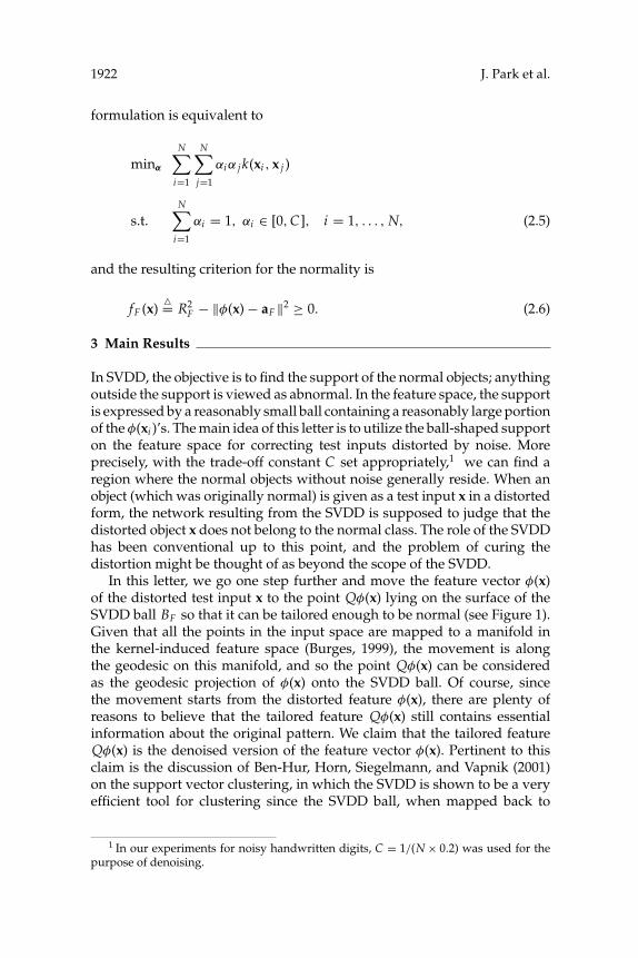
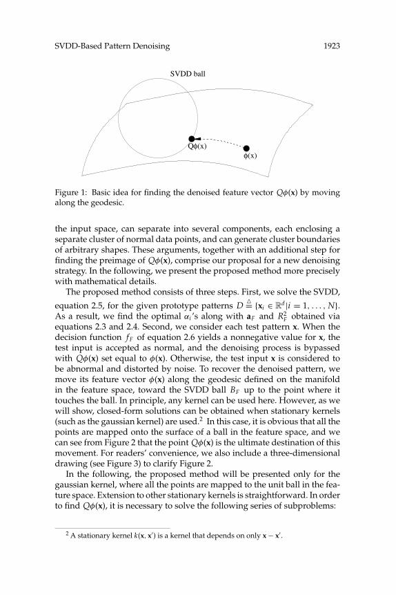
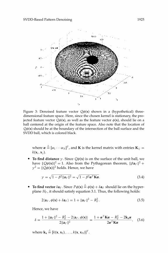
F obtained viaequations 2.3 and 2.4. Second, we consider each test pattern x. When thedecision function fF of equation 2.6 yields a nonnegative value for x, thetest input is accepted as normal, and the denoising process is bypassedwith Qφ(x) set equal to φ(x). Otherwise, the test input x is considered tobe abnormal and distorted by noise. To recover the denoised pattern, wemove its feature vector φ(x) along the geodesic defined on the manifoldin the feature space, toward the SVDD ball BF up to the point where ittouches the ball. In principle, any kernel can be used here. However, as wewill show, closed-form solutions can be obtained when stationary kernels(such as the gaussian kernel) are used.2 In this case, it is obvious that all thepoints are mapped onto the surface of a ball in the feature space, and wecan see from Figure 2 that the point Qφ(x) is the ultimate destination of thismovement. For readers’ convenience, we also include a three-dimensionaldrawing (see Figure 3) to clarify Figure 2.

In the following, the proposed method will be presented only for thegaussian kernel, where all the points are mapped to the unit ball in the fea-ture space. Extension to other stationary kernels is straightforward. In orderto find Qφ(x), it is necessary to solve the following series of subproblems:

2 A stationary kernel k(x, x′) is a kernel that depends on only x − x′.

1924 J. Park et al.

aF

δaF

φ(x) Qφ(x)

βaF

γ

HF

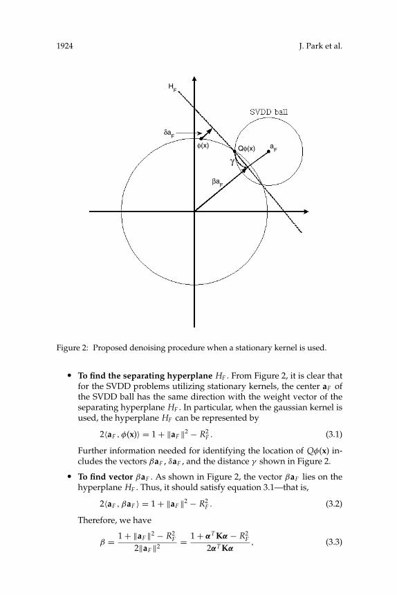
Figure 2: Proposed denoising procedure when a stationary kernel is used.

� To find the separating hyperplane HF . From Figure 2, it is clear thatfor the SVDD problems utilizing stationary kernels, the center aF ofthe SVDD ball has the same direction with the weight vector of theseparating hyperplane HF . In particular, when the gaussian kernel isused, the hyperplane HF can be represented by

2〈aF , φ(x)〉 = 1 + ‖aF ‖2 − R2F . (3.1)

Further information needed for identifying the location of Qφ(x) in-cludes the vectors βaF , δaF , and the distance γ shown in Figure 2.

� To find vector βaF . As shown in Figure 2, the vector βaF lies on thehyperplane HF . Thus, it should satisfy equation 3.1—that is,

2〈aF , βaF 〉 = 1 + ‖aF ‖2 − R2F . (3.2)

Therefore, we have

β = 1 + ‖aF ‖2 − R2F

2‖aF ‖2 = 1 + αT Kα − R2F

2αT Kα, (3.3)


Figure 3: Denoised feature vector Qφ(x) shown in a (hypothetical) three-dimensional feature space. Here, since the chosen kernel is stationary, the pro-jected feature vector Qφ(x), as well as the feature vector φ(x), should lie on aball centered at the origin of the feature space. Also note that the location ofQφ(x) should be at the boundary of the intersection of the ball surface and theSVDD ball, which is colored black.

where α= [α1 · · · αN]T , and K is the kernel matrix with entries Ki j =

k(xi , x j ).� To find distance γ . Since Qφ(x) is on the surface of the unit ball, we

have ‖Qφ(x)‖2 = 1. Also from the Pythagorean theorem, ‖βaF ‖2 +γ 2 = ‖Qφ(x)‖2 holds. Hence, we have

γ =√

1 − β2‖aF ‖2 =√

1 − β2αT Kα. (3.4)

� To find vector δaF . Since Pφ(x)= φ(x) + δaF should lie on the hyper-

plane HF , it should satisfy equation 3.1. Thus, the following holds:

2〈aF , φ(x) + δaF 〉 = 1 + ‖aF ‖2 − R2F . (3.5)

Hence, we have

δ = 1 + ‖aF ‖2 − R2F − 2〈aF , φ(x)〉

2‖aF ‖2 = 1 + αT Kα − R2F − 2kxα

2αT Kα, (3.6)

where kx= [k(x, x1), . . . , k(x, xN)]T .

1926 J. Park et al.

� To find the denoised feature vector Qφ(x). From Figure 2, we see that

Qφ(x) = βaF + γ

‖φ(x) + (δ − β)aF ‖ (φ(x) + (δ − β)aF ). (3.7)

Note that with

λ1= γ

‖φ(x) + (δ − β)aF ‖ (3.8)

and

λ2= β + γ (δ − β)

‖φ(x) + (δ − β)aF ‖ , (3.9)

the above expression for Qφ(x) can be further simplified into

Qφ(x) = λ1φ(x) + λ2aF , (3.10)

where λ1 and λ2 can be computed from

λ1 = γ√1 + 2(δ − β)kxα + (δ − β)2αT Kα

, (3.11)

λ2 = β + γ (δ − β)√1 + 2(δ − β)kxα + (δ − β)2αT Kα

. (3.12)

Obviously, the movement from the feature φ(x) to Qφ(x) is along thegeodesic to the noise-free normal class and thus can be interpreted as per-forming denoising in the feature space. With this interpretation in mind,the feature vector Qφ(x) will be called the denoised feature of x in this letter.In the third and final steps, we try to find the preimage of the denoised fea-ture Qφ(x). If the inverse map φ−1 : F → R

d is well defined and available,this final step attempting to get the denoised pattern via x = φ−1(Qφ(x))will be trivial. However, the exact preimage typically does not exist (Mikaet al., 1999). Thus, we need to seek an approximate solution instead. Forthis, we follow the strategy of Kwok and Tsang (2004), which uses a sim-ple relationship between feature-space distance and input-space distance(Williams, 2002) together with the MDS (multi-dimensional scaling) (Cox& Cox, 2001). Using the kernel trick and the simple relation, equation 3.10,we see that 〈Qφ(x), φ(xi )〉 can be easily computed as follows:

〈Qφ(x), φ(xi )〉 = λ1k(xi , x) + λ2

N∑j=1

α j k(xi , x j ). (3.13)

Thus, the feature space distance between Qφ(x) and φ(xi ) can be obtainedby plugging equation 3.13 into

d2(Qφ(x), φ(xi ))= ‖Qφ(x) − φ(xi )‖2

= 2 − 2〈Qφ(x), φ(xi )〉. (3.14)


Now, note that for the gaussian kernel, the following simple relation-

ship holds true between d(xi , x j )= ‖xi − x j‖ and d(φ(xi ), φ(x j ))

= ‖φ(xi ) −φ(x j )‖ (Williams, 2002):

d2(φ(xi ), φ(x j )) = ‖φ(xi ) − φ(x j )‖2

= 2 − 2k(xi , x j )

= 2 − 2 exp(−‖xi − x j‖2/s2)

= 2 − 2 exp(−d2(xi , x j )/s2). (3.15)

Since the feature space distance d2(Qφ(x), φ(xi )) is now available from equa-tion 3.14 for each training pattern xi , we can easily obtain the correspondinginput space distance between the desired approximate preimage x of Qφ(x)and each xi . Generally, the distances with neighbors are the most importantin determining the location of any point. Hence, here we consider only thesquared input space distances between Qφ(x) and its n nearest neighbors{φ(x(1)), . . . , φ(x(n))} ⊂ DF , and define

d2 = [d21 , d2

2 , . . . , d2n]T , (3.16)

where di is the input space distance between the desired preimage of Qφ(x)and x(i). In MDS (Cox & Cox, 2001), one attempts to find a representationof the objects that preserves the dissimilarities between each pair of them.Thus, we can use the MDS idea to embed Qφ(x) back to the input space.For this, we first take the average of the training data {x(1), . . . , x(n)} ⊂ D toget their centroid x = (1/n)

∑ni=1 x(i), and construct the d × n matrix,

X= [x(1), x(2), . . . , x(n)]. (3.17)

Here, we note that by defining the n × n centering matrix H= In −

(1/n)1n1Tn , where In

= diag[1, . . . , 1] ∈ Rn×n and 1n

= [1, . . . , 1]T ∈ Rn×1, the

matrix XH centers the x(i)’s at their centroid:

XH = [x(1) − x, . . . , x(n) − x]. (3.18)

The next step is to define a coordinate system in the column space ofXH. When XH is of rank q , we can obtain the SVD (singular value

1928 J. Park et al.

decomposition) (Moon & Stirling, 2000) of the d × n matrix XH as

XH = [U1U2]

[�1 0

0 0

] [VT

1

VT2

]

= U1�1VT1

= U1Z, (3.19)

where U1 = [e1, . . . , eq ] is the d × q matrix with orthonormal columns ei ,and Z

= �1VT1 = [z1, . . . , zn] is a q × n matrix with columns zi being the

projections of x(i) − x onto the e j ’s. Note that

‖x(i) − x‖2 = ‖zi‖2, i = 1, . . . , n, (3.20)

and collect these into an n-dimensional vector:

d20

= [‖z1‖2, . . . , ‖zn‖2]T . (3.21)

The location of the preimage x is obtained by requiring d2(x, x(i)), i =1, . . . , n to be as close to those values in equation 3.16 as possible; thus,we need to solve the LS (least squares) problem to find x:

d2(x, x(i)) � d2i , i = 1, . . . , n. (3.22)

Now following the steps of Kwok and Tsang (2004) and Gower (1968),z ∈ R

n×1 defined by x − x = U1z can be shown to satisfy

z = −12�−1

1 VT1

(d2 − d2

0

). (3.23)

Therefore, by transforming equation 3.23 back to the original coordinatedsystem in the input space, the location of the recovered denoised patternturns out to be

x = U1z + x. (3.24)

4 Experiments

In this section, we compare the performance of the proposed method withother denoising methods on toy and real-world data sets. For simplicity, wedenote the proposed method by SVDD.


4.1 Toy Data Set. We first use a toy example to illustrate the proposedmethod and compare its reconstruction performance with PCA. The setup issimilar to that in Mika et al. (1999). Eleven clusters of samples are generatedby first choosing 11 independent sources randomly in [−1, 1]10 and thendrawing samples uniformly from translations of [−σ0, σ0]10 centered at eachsource. For each source, 30 points are generated to form the training dataand 5 points to form the clean test data. Normally distributed noise, withvariance σ 2

o in each component, is then added to each clean test data pointto form the corrupted test data.

We carried out SVDD (with C = 1N×0.6 ) and PCA for the training set,

and then performed reconstructions of each corrupted test point usingboth the proposed SVDD-based method (with neighborhood size n = 10)and the standard PCA method.3 The procedure was repeated for differentnumbers of principal components in PCA and for different values of σ0.For the width s of the gaussian kernel, we used s2 = 2 × 10 × σ 2

0 as in Mikaet al. (1999). From the simulations, we found out that when the input spacedimensionality d is low (as in this example, where d = 10), applying theproposed method iteratively (i.e., recursively applying the denoising to theprevious denoised results) can improve the performance.

We compared the results of our method (with 100 iterations) to those ofthe PCA-based method using the mean squared distance (MSE), which isdefined as

MSE= 1

M

M∑k=1

‖tk − tk‖2, (4.1)

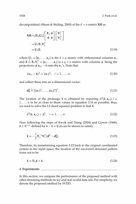
where M is the number of test patterns, tk is the kth clean test pattern, andtk is the denoised result for the kth noisy test pattern. Table 1 shows theratio of MSEPC A/MSESVDD. Note that ratios larger than one indicate thatthe proposed SVDD-based method performs better compared to the otherone.

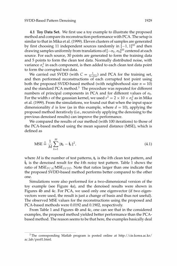
Simulations were also performed for a two-dimensional version of thetoy example (see Figure 4a), and the denoised results were shown inFigures 4b and 4c. For PCA, we used only one eigenvector (if two eigen-vectors were used, the result is just a change of basis and thus not useful).The observed MSE values for the reconstructions using the proposed andPCA-based methods were 0.0192 and 0.1902, respectively.

From Table 1 and Figures 4b and 4c, one can see that in the consideredexamples, the proposed method yielded better performance than the PCA-based method. The reason seems to be that here, the examples basically deal

3 The corresponding Matlab program is posted online at http://cie.korea.ac.kr/ac lab/pro01.html.

1930 J. Park et al.

Table 1: Comparison of MSE Ratios After Reconstructing the Corrupted TestPoints in R

10.

#EV=1 #EV=3 #EV=5 #EV=7 #EV=9

σ0 = 0.05 193.6 91.90 37.37 12.44 2.528σ0 = 0.10 49.36 23.85 10.51 4.667 2.421σ0 = 0.15 22.71 11.34 5.613 3.241 2.419σ0 = 0.20 13.13 6.853 3.854 2.705 2.392

Note: Performance ratios, MSEPC A/MSESVDD, being larger than one, indicate howmuch better SVDD did compared to PCA for different choices of σ0, and differentnumbers of principal components (#EV) in reconstruction using PCA.

−1 −0.5 0 0.5 1

−0.5

0

0.5

1

−1 −0.5 0 0.5 1

−0.5

0

0.5

1

−1 −0.5 0 0.5 1

−0.5

0

0.5

1

Figure 4: A two-dimensional version of the toy example (with σ0 = 0.15) andits denoised results. Lines join each corrupted point (denoted +) with itsreconstruction (denoted o). For SVDD, s2 = 2 × 2 × σ 2

0 and C = 1/(N × 0.6).(a) Training data (denoted •) and corrupted test data (denoted +). (b) Recon-struction using the proposed method (with 100 iterations) along with the resul-tant SVDD balls. (c) Reconstruction using the PCA-based method, where oneprincipal component was used.


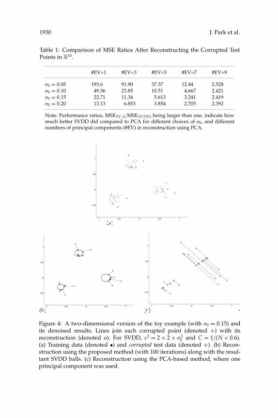
(a)

(d) (e)

(b) (c)

Figure 5: Sample USPS digit images. (a) Clean. (b) With gaussian noise (σ 2 =0.3). (c) With gaussian noise (σ 2 = 0.6). (d) With salt-and-pepper noise (p = 0.3).(e) With salt-and-pepper noise (p = 0.6).

with clustering-type tasks, so any reconstruction method directly utilizingprojection onto low-dimensional linear manifolds would be inefficient.

4.2 Handwritten Digit Data. In this section, we report the denoising re-sults on the USPS digit database (http://www.kernel-machines.org), whichconsists of 16 × 16 handwritten digits of 0 to 9. We first normalized eachfeature value to the range [0, 1]. For each digit, we randomly chose 60 exam-ples to form the training set and 100 examples as the test set (see Figure 5).Two types of additive noise were added to the test set.

The first is the gaussian noise N(0, σ 2) with variance σ 2, and the secondis the so-called salt-and-pepper noise with noise level p, where p/2 is theprobability that a pixel flips to black or white. Denoising was applied toeach digit separately. The width s of the gaussian kernel is set to

s20 = 1

N(N − 1)

N∑i=1

N∑j=1

‖xi − x j‖2, (4.2)

the average squared distance between training patterns. Here, the value ofC was set to the effect that the support for the normal class resulting fromthe SVDD may cover approximately 80% (=100% − 20%) of the trainingdata. Finally, in the third step, we used n = 10 neighbors to recover thedenoised pattern x by solving the preimage problem.

1932 J. Park et al.

0 10 20 30 40 50 601.5

2

2.5

3

3.5

4

4.5

5

#EVs

SN

R (

in d

B)

SVDDKPCA (Mika et. al.)KPCA (Kwok & Tsang)PCAWavelet (VisuShrink)Wavelet (SureShrink)

(a)

0 10 20 30 40 50 601.5

2

2.5

3

3.5

4

4.5

5

#EVs

SN

R (

in d

B)


(b)

0 10 20 30 40 50 602

2.5

3

3.5

4

4.5

5

5.5

#EVs

SN

R (

in d

B)


(c)

0 10 20 30 40 50 601

1.5

2

2.5

3

3.5

4

4.5

#EVs

SN

R (

in d

B)


(d)0 10 20 30 40 50 60

1.5

2

2.5

3

3.5

4

4.5

5

#EVs

SN

R (

in d

B)


(e)0 10 20 30 40 50 60

2

2.5

3

3.5

4

4.5

5

#EVs

SN

R (

in d

B)


(f)

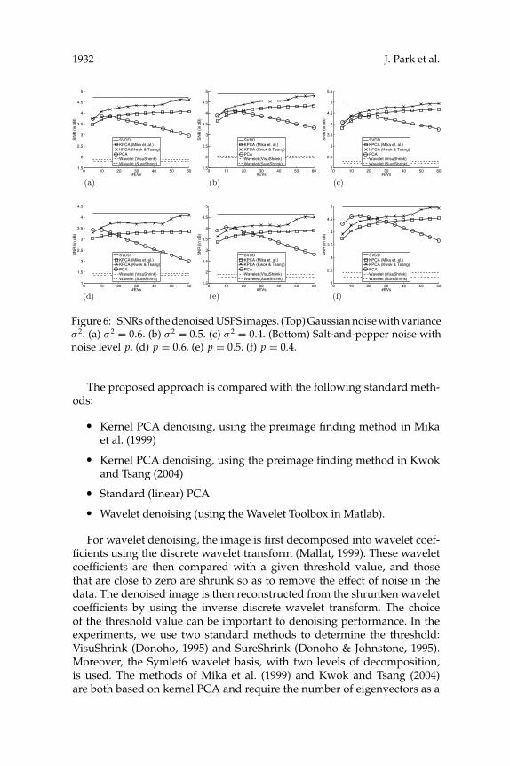
Figure 6: SNRs of the denoised USPS images. (Top) Gaussian noise with varianceσ 2. (a) σ 2 = 0.6. (b) σ 2 = 0.5. (c) σ 2 = 0.4. (Bottom) Salt-and-pepper noise withnoise level p. (d) p = 0.6. (e) p = 0.5. (f) p = 0.4.

The proposed approach is compared with the following standard meth-ods:

� Kernel PCA denoising, using the preimage finding method in Mikaet al. (1999)

� Kernel PCA denoising, using the preimage finding method in Kwokand Tsang (2004)

� Standard (linear) PCA� Wavelet denoising (using the Wavelet Toolbox in Matlab).

For wavelet denoising, the image is first decomposed into wavelet coef-ficients using the discrete wavelet transform (Mallat, 1999). These waveletcoefficients are then compared with a given threshold value, and thosethat are close to zero are shrunk so as to remove the effect of noise in thedata. The denoised image is then reconstructed from the shrunken waveletcoefficients by using the inverse discrete wavelet transform. The choiceof the threshold value can be important to denoising performance. In theexperiments, we use two standard methods to determine the threshold:VisuShrink (Donoho, 1995) and SureShrink (Donoho & Johnstone, 1995).Moreover, the Symlet6 wavelet basis, with two levels of decomposition,is used. The methods of Mika et al. (1999) and Kwok and Tsang (2004)are both based on kernel PCA and require the number of eigenvectors as a


(a) (b) (c)

(d) (e) (f)

(g) (h) (i)

(j) (k) (l)

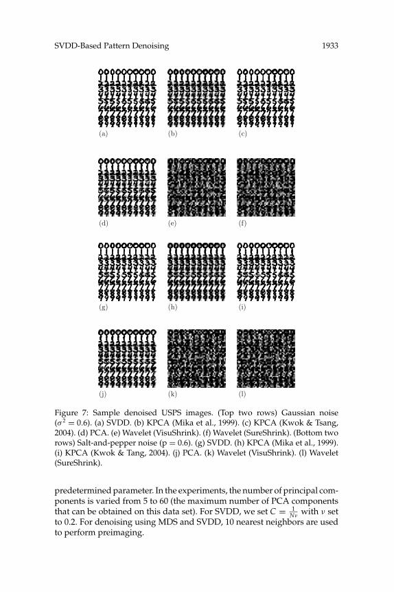
Figure 7: Sample denoised USPS images. (Top two rows) Gaussian noise(σ 2 = 0.6). (a) SVDD. (b) KPCA (Mika et al., 1999). (c) KPCA (Kwok & Tsang,2004). (d) PCA. (e) Wavelet (VisuShrink). (f) Wavelet (SureShrink). (Bottom tworows) Salt-and-pepper noise (p = 0.6). (g) SVDD. (h) KPCA (Mika et al., 1999).(i) KPCA (Kwok & Tang, 2004). (j) PCA. (k) Wavelet (VisuShrink). (l) Wavelet(SureShrink).

predetermined parameter. In the experiments, the number of principal com-ponents is varied from 5 to 60 (the maximum number of PCA componentsthat can be obtained on this data set). For SVDD, we set C = 1

Nνwith ν set

to 0.2. For denoising using MDS and SVDD, 10 nearest neighbors are usedto perform preimaging.

1934 J. Park et al.

0 50 100 150 200 250 3000

1

2

3

4

5

6

#EVs

SN

R (

in d

B)


(a)

0 50 100 150 200 250 3000

1

2

3

4

5

6

#EVs

SN

R (

in d

B)


(b)

0 50 100 150 200 250 3001

2

3

4

5

6

7

#EVs

SN

R (

in d

B)


(c)

0 50 100 150 200 250 300−2

−1

0

1

2

3

4

5

#EVs

SN

R (

in d

B)


(d)0 50 100 150 200 250 300

−2

−1

0

1

2

3

4

5

#EVs

SN

R (

in d

B)


(e)0 50 100 150 200 250 300

0

1

2

3

4

5

6

7

#EVs

SN

R (

in d

B)


(f)

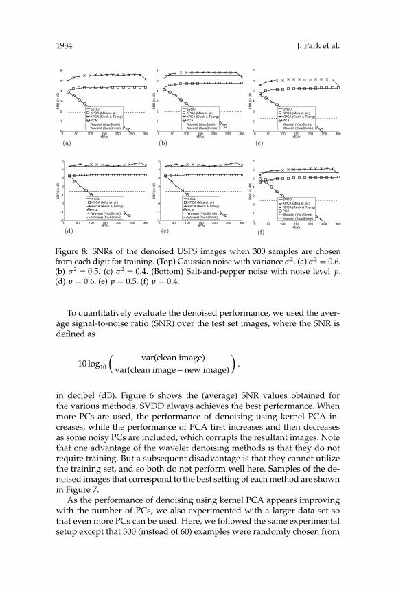
Figure 8: SNRs of the denoised USPS images when 300 samples are chosenfrom each digit for training. (Top) Gaussian noise with variance σ 2. (a) σ 2 = 0.6.(b) σ 2 = 0.5. (c) σ 2 = 0.4. (Bottom) Salt-and-pepper noise with noise level p.(d) p = 0.6. (e) p = 0.5. (f) p = 0.4.

To quantitatively evaluate the denoised performance, we used the aver-age signal-to-noise ratio (SNR) over the test set images, where the SNR isdefined as

10 log10

(var(clean image)

var(clean image – new image)

),

in decibel (dB). Figure 6 shows the (average) SNR values obtained forthe various methods. SVDD always achieves the best performance. Whenmore PCs are used, the performance of denoising using kernel PCA in-creases, while the performance of PCA first increases and then decreasesas some noisy PCs are included, which corrupts the resultant images. Notethat one advantage of the wavelet denoising methods is that they do notrequire training. But a subsequent disadvantage is that they cannot utilizethe training set, and so both do not perform well here. Samples of the de-noised images that correspond to the best setting of each method are shownin Figure 7.

As the performance of denoising using kernel PCA appears improvingwith the number of PCs, we also experimented with a larger data set sothat even more PCs can be used. Here, we followed the same experimentalsetup except that 300 (instead of 60) examples were randomly chosen from


0.1 0.2 0.3 0.4 0.5 0.64.4

4.6

4.8

5

5.2

5.4

ν

SN

R (

in d

B)

σ2=0.3

σ2=0.4

σ2=0.5

σ2=0.6

(a)0 2 4 6 8

4

4.5

5

5.5

weighting factor for s2

SN

R (

in d

B)

σ2=0.3

σ2=0.4

σ2=0.5

σ2=0.6

(b)

6 8 10 12 144.4

4.6

4.8

5

5.2

5.4

n

SN

R (

in d

B)

σ2=0.3

σ2=0.4

σ2=0.5

σ2=0.6

(c)

0.1 0.2 0.3 0.4 0.5 0.63.5

4

4.5

5

5.5

6

ν

SN

R (

in d

B)

p=0.3p=0.4p=0.5p=0.6

(d)0 2 4 6 8

3.5

4

4.5

5

5.5

6

weighting factor for s2

SN

R (

in d

B)

p=0.3p=0.4p=0.5p=0.6

(e)6 8 10 12 14

3.8

4

4.2

4.4

4.6

4.8

5

5.2

5.4

n

SN

R (

in d

B)

p=0.3p=0.4p=0.5p=0.6

(f)

Figure 9: SNR results of the proposed method on varying each of ν, width of thegaussian kernel (s) and the neighborhood size for MDS (n). (Top) Gaussian noisewith different σ 2’s. (a) Varying ν. (b) Varying s as a factor of s0 in equation 4.2.(c) Varying n. (Bottom) Salt-and-pepper noise with different p’s. (d) Varying ν.(e) Varying s as a factor of s0 in equation 4.2. (f) Varying n.

each digit to form the training set. Figure 8 shows the SNR values for thevarious methods. On this larger data set, denoising using kernel PCA doesperform better than the others when a suitable number of PCs are chosen.This demonstrates that the proposed denoising procedure is comparativelymore effective on small training sets.

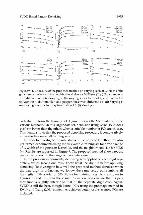
In order to investigate the robustness of the proposed method, we alsoperformed experiments using the 60-example training set for a wide rangeof ν, width of the gaussian kernel (s), and the neighborhood size for MDS(n). Results are reported in Figure 9. The proposed method shows robustperformance around the range of parameters used.

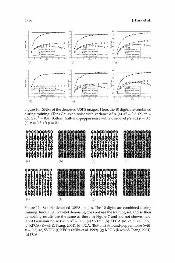
In the previous experiments, denoising was applied to each digit sep-arately, which means one must know what the digit is before applyingdenoising. To investigate how well the proposed method denoises whenthe true digit is unknown, we follow the same setup but combine allthe digits (with a total of 600 digits) for training. Results are shown inFigures 10 and 11. From the visual inspection, one can see that its per-formance is slightly inferior to that of the separate digit case. Again,SVDD is still the best, though kernel PCA using the preimage method inKwok and Tsang (2004) sometimes achieves better results as more PCs areincluded.

1936 J. Park et al.

0 10 20 30 40 50 601.5

2

2.5

3

3.5

4

4.5

5

#EVs

SN

R (

in d

B)


(a)

0 10 20 30 40 50 601.5

2

2.5

3

3.5

4

4.5

5

5.5

#EVs

SN

R (

in d

B)


(b)

0 10 20 30 40 50 602

2.5

3

3.5

4

4.5

5

5.5

#EVs

SN

R (

in d

B)


(c)

0 10 20 30 40 50 601

1.5

2

2.5

3

3.5

4

4.5

#EVs

SN

R (

in d

B)


(d)0 10 20 30 40 50 60

1.5

2

2.5

3

3.5

4

4.5

5

#EVs

SN

R (

in d

B)


(e)0 10 20 30 40 50 60

2

2.5

3

3.5

4

4.5

5

5.5

#EVs

SN

R (

in d

B)


(f)

Figure 10: SNRs of the denoised USPS images. Here, the 10 digits are combinedduring training. (Top) Gaussian noise with variance σ 2’s. (a) σ 2 = 0.6. (b) σ 2 =0.5. (c) σ 2 = 0.4. (Bottom) Salt-and-pepper noise with noise level p’s. (d) p = 0.6.(e) p = 0.5. (f) p = 0.4.

(a) (b) (c) (d)

(e) (f) (g) (h)

Figure 11: Sample denoised USPS images. The 10 digits are combined duringtraining. Recall that wavelet denoising does not use the training set, and so theirde-noising results are the same as those in Figure 7 and are not shown here.(Top) Gaussian noise (with σ 2 = 0.6). (a) SVDD. (b) KPCA (Mika et al. 1999).(c) KPCA (Kwok & Tsang, 2004). (d) PCA. (Bottom) Salt-and-pepper noise (withp = 0.6). (e) SVDD. (f) KPCA (Mika et al. 1999). (g) KPCA (Kwok & Tsang, 2004).(h) PCA.


5 Conclusion

We have addressed the problem of pattern denoising based on the SVDD.Along with a brief review over the SVDD, we presented a new denoisingmethod that uses the SVDD, the geodesic projection of the noisy point tothe surface of the SVDD ball in the feature space, and a method for findingthe preimage of the denoised feature vectors. Work yet to be done includesmore extensive comparative studies, which will reveal the strengths andweaknesses of the proposed method, and refinement of the method forbetter denoising.

References

Ben-Hur, A., Horn D., Siegelmann H. T., & Vapnik V. (2001). Support vector cluster-ing. Journal of Machine Learning Research, 2, 125–137.

Burges, C. J. C. (1999). Geometry and invariance in kernel based methods. In A. J.Smola, P. L. Bartlett, B. Scholkopf, & D. Schuurmons (Eds.), Advances in kernelmethods—support vector learning. Cambridge, MA: MIT Press.

Campbell, C., & Bennett, K. P. (2001). A linear programming approach to nov-elty detection. In T. K. Leen, T. G. Dietterich, & V. Tresp (Eds.), Advances inneural information processing systems, 13, (pp. 395–401). Cambridge, MA: MITPress.

Cox, T. F., & Cox, M. A. A. (2001). Multidimensional scaling (2nd ed.). London: Chap-man & Hall.

Crammer, K., & Chechik, G. (2004). A needle in a haystack: Local one-class optimiza-tion. In Proceedings of the Twenty-First International Conference on Machine Learning.Banff, Alberta, Canada.

Cristianini, N., & Shawe-Taylor, J. (2000). An introduction to support vector machinesand other kernel-based learning methods. Cambridge: Cambridge University Press.

Donoho, D. L. (1995). De-noising by soft-thresholding. IEEE Transactions on Informa-tion Theory, 41(3), 613–627.

Donoho, D. L., & Johnstone, I. M. (1995). Adapting to unknown smoothness viawavelet shrinkage. Journal of the American Statistical Association, 90(432), 1200–1224.

Gower, J. C. (1968). Adding a point to vector diagrams in multivariate analysis.Biometrika, 55(3), 582–585.

Kwok, J. T., & Tsang, I. W. (2004). The pre-image problem in kernel methods. IEEETransactions on Neural Networks, 15(6), 1517–1525.

Lanckriet, G. R. G., El Ghaoui, L., & Jordan, M. I. (2003). Robust novelty detectionwith single-class MPM. In S. Becker, S. Thron, & K. Obermayer (Eds.), Advancesin neural information processing systems, 15, (pp. 905–912). Cambridge, MA: MITPress.

Laskov, P., Schafer, C., & Kotenko, I. (2004). Intrusion detection in unlabeled data withquarter-sphere support vector machines. In Proceeding of Detection of Intrusionsand Malware and Vulnerability Assessment (DIMVA) 2004 (pp. 71–82). Dortmund,Germany.

1938 J. Park et al.

Mallat, S. G. (1999). A wavelet tour of signal processing (2nd ed.). San Diego, CA:Academic Press.

Mika, S., Scholkopf, B., Smola, A. J., Muller, K. R., Scholz, M., & Ratsch, G. (1999).Kernel PCA and de-noising in feature space. In M. S. Kearns, S. Solla, & D.Cohn (Eds.), Advances in neural information processing systems, 11 (pp. 536–542).Cambridge, MA: MIT Press.

Moon, T. K., & Stirling, W. C. (2000). Mathematical methods and algorithms for signalprocessing. Upper Saddle River, NJ: Prentice Hall.

Muller, K.-R., Mika, S., Ratsch, G., Tsuda, K., & Scholkopf, B. (2001). An introductionto kernel-based learning algorithms. IEEE Transactions on Neural Networks, 12(2),181–201.

Pekalska, E., Tax, D. M. J., & Duin, R. P. W. (2003). One-class LP classifiers for dissim-ilarity representations. In S. Becker, S. Thrun, & K. Obermayer (Eds.) Advancesin neural information processing systems, 15 (pp. 761–768). Cambridge, MA: MITPress.

Ratsch, G., Mika, S., Scholkopf, B., & Muller, K.-R. (2002). Constructing boosting al-gorithms from SVMs: An application to one-class classification. IEEE Transactionson Pattern Analysis and Machine Intelligence, 24(9), 1184–1199.

Scholkopf, B., Mika, S., Burges, C., Knirsch, P., Muller, K.-R., Ratsch, G., & Smola, A. J.(1999). Input space vs feature space in kernel-based methods. IEEE Transactionson Neural Networks, 10(5), 1000–1017.

Scholkopf, B., Platt, J. C., Shawe-Taylor, J., Smola, A. J., & Williamson, R. C. (2001).Estimating the support of a high-dimensional distribution. Neural Computation,13(7), 1443–1471.

Scholkopf, B., Platt, J. C., & Smola, A. J. (2000). Kernel method for percentile featureextraction (Tech. Rep. MSR-TR-2000-22). Redmond, WA: Microsoft Research.

Scholkopf, B., & Smola, A. J. (2002). Learning with kernels, Cambridge, MA: MIT Press.Tax, D. (2001). One-class classification. Unpublished doctoral/dissertation, Delft Uni-

versity of Technology.Tax, D., & Duin, R. (1999). Support vector data description. Pattern Recognition Letters,

20(11–13), 1191–1199.Williams, C. K. I. (2002). On a connection between kernel PCA and metric multidi-

mensional scaling. Machine Learning, 46(1–3), 11–19.

Received August 31, 2005; accepted October 30, 2006.

SVDD-Based Pattern Denoising

Documents