SUSTAINABLE WORLDWIDE TRANSPORTATION

SWT-2017-12 AUGUST 2017

SENSOR FUSION: A COMPARISON OF SENSING CAPABILITIES OF HUMAN DRIVERS AND

HIGHLY AUTOMATED VEHICLES

BRANDON SCHOETTLE

SUSTAINABLE WORLDWIDETRANSPORTATION

SENSOR FUSION: A COMPARISON OF SENSING CAPABILITIES

OF HUMAN DRIVERS AND HIGHLY AUTOMATED VEHICLES

Brandon Schoettle

The University of Michigan Sustainable Worldwide Transportation

Ann Arbor, Michigan 48109-2150 U.S.A.

Report No. SWT-2017-12 August 2017

i

Technical Report Documentation Page 1. Report No.

SWT-2017-12 2. Government Accession No.

3. Recipient’s Catalog No.

4. Title and Subtitle Sensor Fusion: A Comparison of Sensing Capabilities of Human Drivers and Highly Automated Vehicles

5. Report Date

August 2017 6. Performing Organization Code

383818 7. Author(s)

Brandon Schoettle 8. Performing Organization Report No. SWT-2017-12

9. Performing Organization Name and Address The University of Michigan Sustainable Worldwide Transportation 2901 Baxter Road Ann Arbor, Michigan 48109-2150 U.S.A.

10. Work Unit no. (TRAIS)

11. Contract or Grant No.

12. Sponsoring Agency Name and Address The University of Michigan Sustainable Worldwide Transportation

13. Type of Report and Period Covered 14. Sponsoring Agency Code

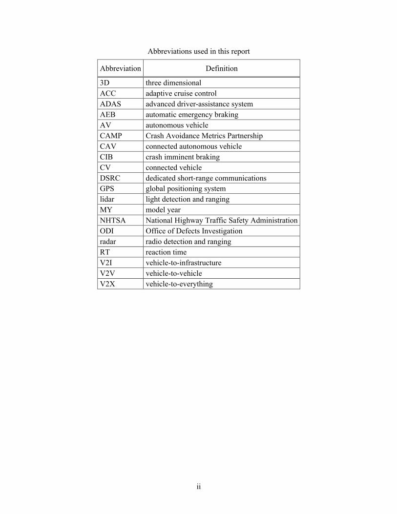
15. Supplementary Notes Information about Sustainable Worldwide Transportation is available at http://www.umich.edu/~umtriswt. 16. Abstract

This white paper analyzes and compares the sensing capabilities of human drivers and highly automated vehicles. The key findings from this study are as follows:

• Machines/computers are generally well suited to perform tasks like driving, especially in regard to reaction time (speed), power output and control, consistency, and multichannel information processing.

• Human drivers still generally maintain an advantage in terms of reasoning, perception, and sensing when driving.

• Matching (or exceeding) human sensing capabilities requires autonomous vehicles (AVs) to employ a variety of sensors, which in turn requires complete sensor fusion across the system, combining all sensor inputs to form a unified view of the surrounding roadway and environment.

• While no single sensor completely equals human sensing capabilities, some offer capabilities not possible for a human driver.

• Integration of connected-vehicle technology extends the effective range and coverage area of both human-driven vehicles and AVs, with a longer operating range and omnidirectional communication that does not require unobstructed line of sight the way human drivers and AVs generally do.

• Combining human-driven vehicles or AVs that can “see” traffic and their environment with connected vehicles (CVs) that can “talk” to other traffic and their environment maximizes potential awareness of other roadway users and roadway conditions.

• AV sensing will still be critical for detection of any road user or roadway obstacle that is not part of the interconnected dedicated short-range communications (DSRC) system used by CVs.

• A fully implemented connected autonomous vehicle offers the best potential to effectively and safely replace the human driver when operating vehicles at NHTSA automation levels 4 and 5. 17. Key Words self-driving, autonomous vehicle, human driver, driver performance, sensing, sensors, radar, lidar, connected vehicle, connected autonomous vehicle

18. Distribution Statement Unlimited

19. Security Classification (of this report) None

20. Security Classification (of this page) None

21. No. of Pages 45

22. Price

ii

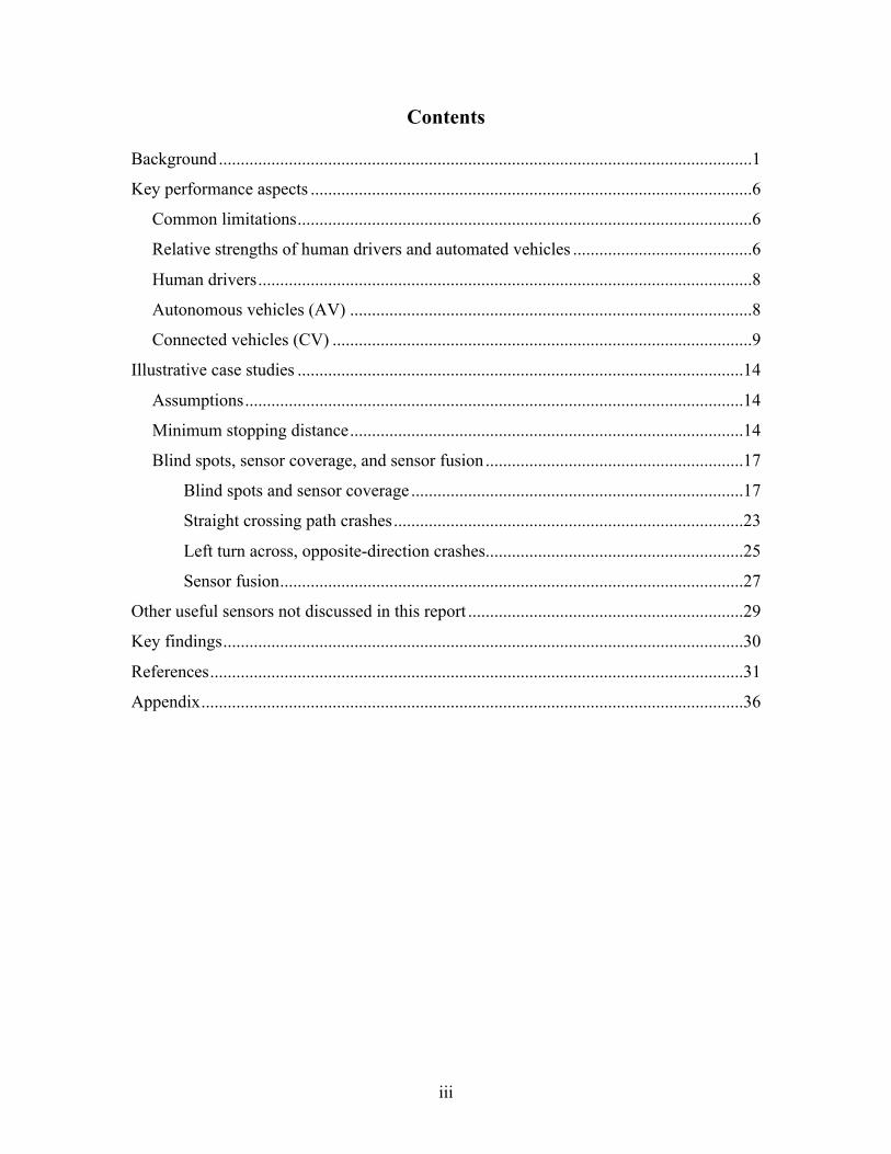
Abbreviations used in this report

Abbreviation Definition

3D three dimensional ACC adaptive cruise control ADAS advanced driver-assistance system AEB automatic emergency braking AV autonomous vehicle CAMP Crash Avoidance Metrics Partnership CAV connected autonomous vehicle CIB crash imminent braking CV connected vehicle DSRC dedicated short-range communications GPS global positioning system lidar light detection and ranging MY model year NHTSA National Highway Traffic Safety Administration ODI Office of Defects Investigation radar radio detection and ranging RT reaction time V2I vehicle-to-infrastructure V2V vehicle-to-vehicle V2X vehicle-to-everything

iii

Contents

Background ..........................................................................................................................1

Key performance aspects .....................................................................................................6

Common limitations ........................................................................................................6

Relative strengths of human drivers and automated vehicles .........................................6

Human drivers .................................................................................................................8

Autonomous vehicles (AV) ............................................................................................8

Connected vehicles (CV) ................................................................................................9

Illustrative case studies ......................................................................................................14

Assumptions ..................................................................................................................14

Minimum stopping distance ..........................................................................................14

Blind spots, sensor coverage, and sensor fusion ...........................................................17

Blind spots and sensor coverage ............................................................................17

Straight crossing path crashes ................................................................................23

Left turn across, opposite-direction crashes ...........................................................25

Sensor fusion ..........................................................................................................27

Other useful sensors not discussed in this report ...............................................................29

Key findings .......................................................................................................................30

References ..........................................................................................................................31

Appendix ............................................................................................................................36

1

Background Fully autonomous vehicles promise to be able to replace the human driver for most if not

all driving situations and scenarios (NHTSA, 2016). To do this efficiently, effectively, and

safely requires a multitude of sensors linked to the overall autonomous (also called self-driving

or driverless) vehicle system. Not only is it essential that such vehicles accurately know where

they are located within the world, they must be equally aware as an alert human driver (but

ideally, significantly more aware) of what is physically located around them and what is

happening around them. This is no easy task considering the extensive range of fixed objects

(signs, light poles, buildings, trees, mailboxes, etc.) and moving objects (vehicles, bicycles,

pedestrians, animals, etc.), other roadway users and pedestrians, and environmental conditions

(especially severe conditions such as rain, snow, fog, etc.). Adding to this challenge is the fact

that most experienced drivers are reasonably capable of anticipating or predicting the behavior of

other roadway users and pedestrians (Anthony, 2016; Lee & Sheppard, 2016; MacAdam, 2003).1

(For additional discussion of these issues, see: Sivak & Schoettle, 2015.)

With 35,092 fatalities on U.S. roadways in 2015, and with 94% of crashes associated

with “a human choice or error” (NHTSA, 2016), implementation of safe, successful automated-

vehicle technology stands to significantly improve safety on U.S. roads. However, to fully

realize substantial improvements in traffic safety will likely require implementation of self-

driving technology across all forms of road transportation. For example, in 2015 there were

more than 12 million large trucks and buses registered in the U.S., and these vehicle types were

involved in crashes resulting in 4,337 fatalities, or about 12% of all traffic fatalities that year

(FMCSA, 2017). In addition to automated systems for everyday light-duty passenger vehicles,

such systems are also being planned or currently in development for other major road users,

including heavy-duty vehicles (Daimler, 2017a; Freedman, 2017), buses (Daimler, 2017b;

Walker, 2015), and taxi-like or ride-hailing services (Ohnsman, 2017).

To sense and guide their way through the world, autonomous vehicles (AVs) will use a

variety of sensors to accomplish this task, each with their own advantages and disadvantages.

Furthermore, certain sensors may be employed to perform multiple tasks. For example, lidar can 1 Fitts (1962): “If we understand how a man performs a function, we will have available a mathematical model which presumably should permit us to build a physical device or program a computer to perform the function in the same way (or in a superior manner). Inability to build a machine that will perform a given function as well as or better than a man, therefore, simply indicates our ignorance of the answers to fundamental problems of psychology.”

2

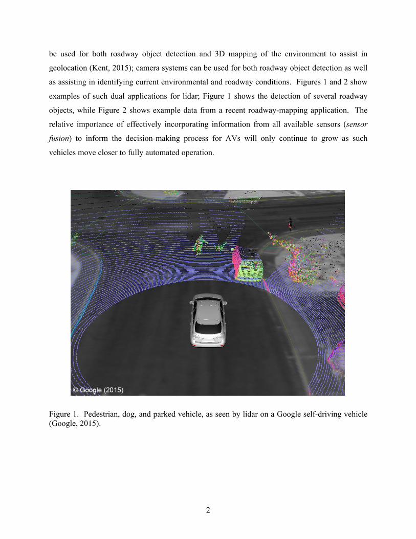
be used for both roadway object detection and 3D mapping of the environment to assist in

geolocation (Kent, 2015); camera systems can be used for both roadway object detection as well

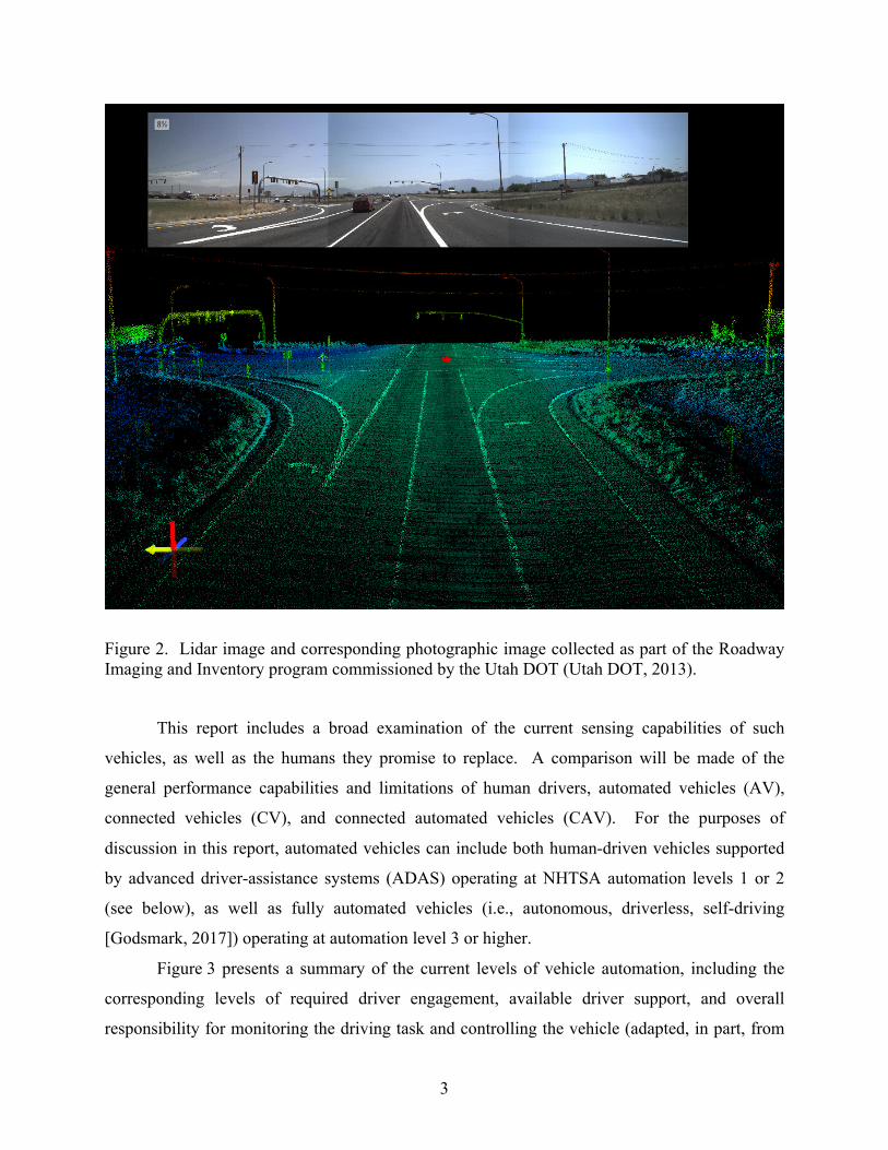
as assisting in identifying current environmental and roadway conditions. Figures 1 and 2 show

examples of such dual applications for lidar; Figure 1 shows the detection of several roadway

objects, while Figure 2 shows example data from a recent roadway-mapping application. The

relative importance of effectively incorporating information from all available sensors (sensor

fusion) to inform the decision-making process for AVs will only continue to grow as such

vehicles move closer to fully automated operation.

Figure 1. Pedestrian, dog, and parked vehicle, as seen by lidar on a Google self-driving vehicle (Google, 2015).

3

Figure 2. Lidar image and corresponding photographic image collected as part of the Roadway Imaging and Inventory program commissioned by the Utah DOT (Utah DOT, 2013).

This report includes a broad examination of the current sensing capabilities of such

vehicles, as well as the humans they promise to replace. A comparison will be made of the

general performance capabilities and limitations of human drivers, automated vehicles (AV),

connected vehicles (CV), and connected automated vehicles (CAV). For the purposes of

discussion in this report, automated vehicles can include both human-driven vehicles supported

by advanced driver-assistance systems (ADAS) operating at NHTSA automation levels 1 or 2

(see below), as well as fully automated vehicles (i.e., autonomous, driverless, self-driving

[Godsmark, 2017]) operating at automation level 3 or higher.

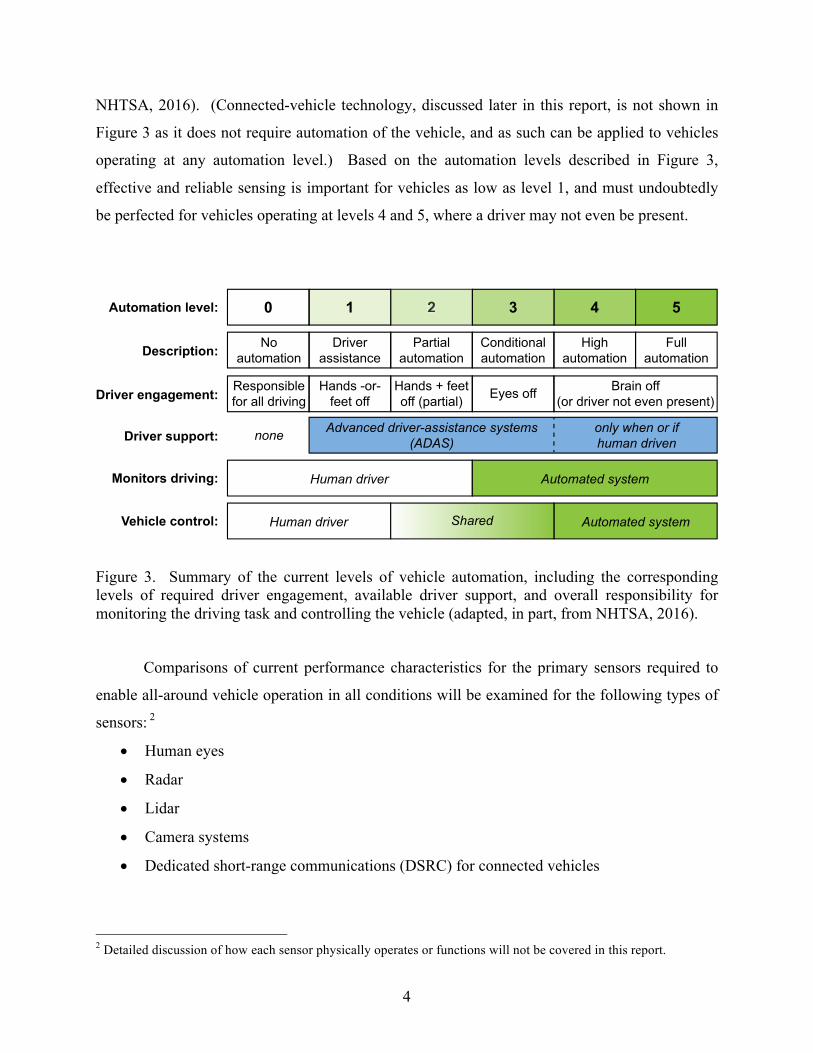
Figure 3 presents a summary of the current levels of vehicle automation, including the

corresponding levels of required driver engagement, available driver support, and overall

responsibility for monitoring the driving task and controlling the vehicle (adapted, in part, from

4

NHTSA, 2016). (Connected-vehicle technology, discussed later in this report, is not shown in

Figure 3 as it does not require automation of the vehicle, and as such can be applied to vehicles

operating at any automation level.) Based on the automation levels described in Figure 3,

effective and reliable sensing is important for vehicles as low as level 1, and must undoubtedly

be perfected for vehicles operating at levels 4 and 5, where a driver may not even be present.

Figure 3. Summary of the current levels of vehicle automation, including the corresponding levels of required driver engagement, available driver support, and overall responsibility for monitoring the driving task and controlling the vehicle (adapted, in part, from NHTSA, 2016).

Comparisons of current performance characteristics for the primary sensors required to

enable all-around vehicle operation in all conditions will be examined for the following types of

sensors: 2

• Human eyes

• Radar

• Lidar

• Camera systems

• Dedicated short-range communications (DSRC) for connected vehicles

2 Detailed discussion of how each sensor physically operates or functions will not be covered in this report.

543210Automation level:

Fullautomation

Highautomation

Conditionalautomation

Partialautomation

Driverassistance

NoautomationDescription:

Human driver Automated systemMonitors driving:

Advanced driver-assistance systems(ADAS)Driver support: none

Automated systemHuman driver SharedVehicle control:

Brain off(or driver not even present)Eyes offHands + feet

off (partial)Hands -or-

feet offResponsiblefor all drivingDriver engagement:

only when or ifhuman driven

5

(Ultrasonic and other short-range sensors are not included in this analysis as they are nearly

exclusively used for low-speed applications such as parking, and are not as critical to safe

vehicle operation at moderate to high speeds as the other sensors examined here. Similarly,

while GPS is integral to geolocation for navigation, it is not a sensor applicable to the

discussion in this report.)

6

Key performance aspects

Common limitations

There are several shared limitations affecting each driver or vehicle type. The following

list, though not exhaustive, identifies some of the most common performance limitations and

related causes:

• Extreme weather (heavy rain, snow, or fog): Reduces maximum range and signal quality

(acuity, contrast, excessive visual clutter) for human vision, AV visual systems (cameras,

lidar), and DSRC transmissions (though to a lesser extent).

• Excessive dirt or physical obstructions (such as snow or ice) on the vehicle: Interferes

with or reduces maximum range and signal quality (acuity, contrast, physical occlusion

of field of view) for human vision and all basic AV sensors (cameras, lidar, radar).

• Darkness or low illumination: Reduces maximum range and signal quality (acuity,

contrast, possible glare from external light sources) for human vision and AV camera

systems.

• Large physical obstructions (buildings, terrain, heavy vegetation, etc.): Interferes with

line of sight for human vision and all basic AV sensors (cameras, radar, lidar); some

obstructions can also reduce the maximum signal range for DSRC.

• Dense traffic: Interferes with or reduces line of sight for human vision and all basic AV

sensors (cameras, radar, lidar); can also interfere with effective DSRC transmission

caused by excessive volumes of signals/messages. (However, human drivers do have

some limited ability to see through the windows of adjacent vehicles.)

Relative strengths of human drivers and automated vehicles

A topic of frequent discussion when designing a system combining human and machine

relates to the question of which tasks are performed best by whom (human versus machine).

(For the purposes of this discussion, the term machine also encompasses computer systems and

combined computer/mechanical systems such as automated vehicles.) A classic analysis by Fitts

(1951) outlined the major categories of strengths and weaknesses for each side of the human-

machine interaction relationship (i.e., ideal function allocation) (also see: Cummings, 2014; de

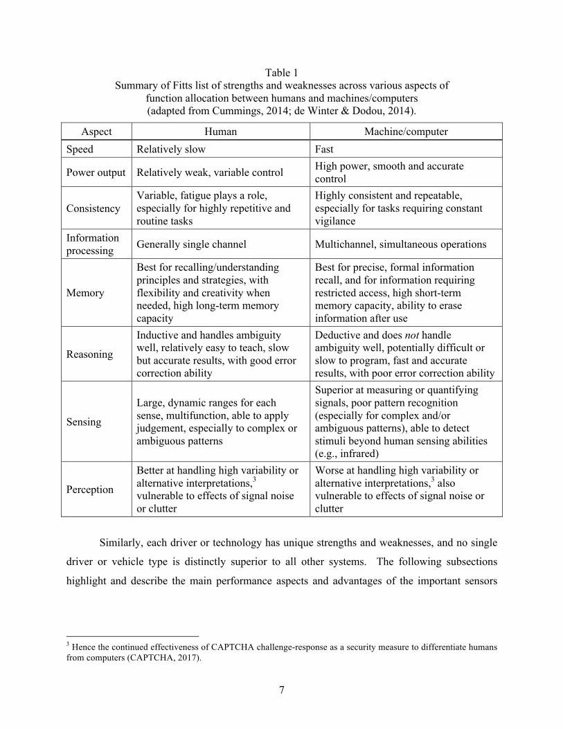
Winter & Dodou, 2014). Table 1 shows a summary of the so-called Fitts list (adapted from

Cummings, 2014; de Winter & Dodou, 2014).

7

Table 1 Summary of Fitts list of strengths and weaknesses across various aspects of

function allocation between humans and machines/computers (adapted from Cummings, 2014; de Winter & Dodou, 2014).

Aspect Human Machine/computer Speed Relatively slow Fast

Power output Relatively weak, variable control High power, smooth and accurate control

Consistency Variable, fatigue plays a role, especially for highly repetitive and routine tasks

Highly consistent and repeatable, especially for tasks requiring constant vigilance

Information processing Generally single channel Multichannel, simultaneous operations

Memory

Best for recalling/understanding principles and strategies, with flexibility and creativity when needed, high long-term memory capacity

Best for precise, formal information recall, and for information requiring restricted access, high short-term memory capacity, ability to erase information after use

Reasoning

Inductive and handles ambiguity well, relatively easy to teach, slow but accurate results, with good error correction ability

Deductive and does not handle ambiguity well, potentially difficult or slow to program, fast and accurate results, with poor error correction ability

Sensing

Large, dynamic ranges for each sense, multifunction, able to apply judgement, especially to complex or ambiguous patterns

Superior at measuring or quantifying signals, poor pattern recognition (especially for complex and/or ambiguous patterns), able to detect stimuli beyond human sensing abilities (e.g., infrared)

Perception

Better at handling high variability or alternative interpretations,3 vulnerable to effects of signal noise or clutter

Worse at handling high variability or alternative interpretations,3 also vulnerable to effects of signal noise or clutter

Similarly, each driver or technology has unique strengths and weaknesses, and no single

driver or vehicle type is distinctly superior to all other systems. The following subsections

highlight and describe the main performance aspects and advantages of the important sensors

3 Hence the continued effectiveness of CAPTCHA challenge-response as a security measure to differentiate humans from computers (CAPTCHA, 2017).

8

associated with each driver or technology.4 While the specific focus of these sections is light-

duty passenger vehicles, automated heavy-duty vehicles employ the same types of sensors, with

generally the same performance characteristics (Daimler, 2014).

Human drivers

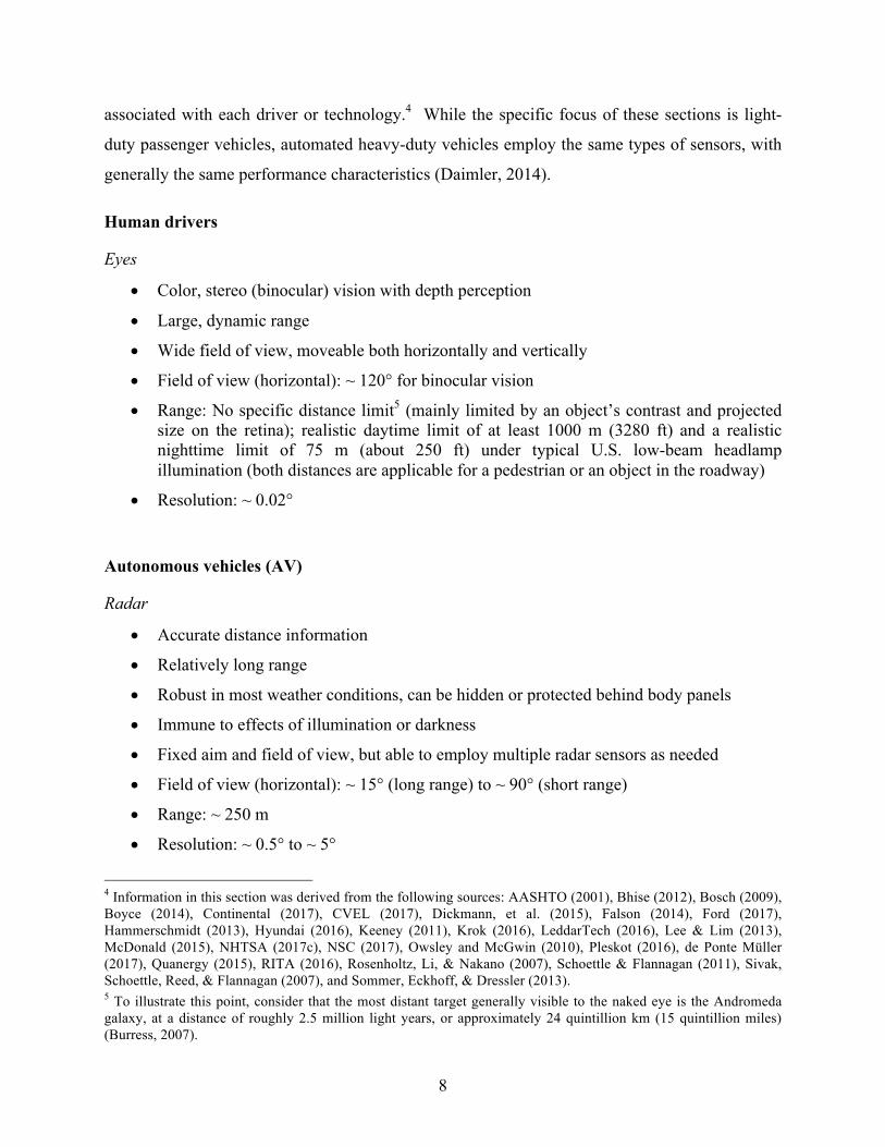
Eyes

• Color, stereo (binocular) vision with depth perception

• Large, dynamic range

• Wide field of view, moveable both horizontally and vertically

• Field of view (horizontal): ~ 120° for binocular vision

• Range: No specific distance limit5 (mainly limited by an object’s contrast and projected size on the retina); realistic daytime limit of at least 1000 m (3280 ft) and a realistic nighttime limit of 75 m (about 250 ft) under typical U.S. low-beam headlamp illumination (both distances are applicable for a pedestrian or an object in the roadway)

• Resolution: ~ 0.02°

Autonomous vehicles (AV)

Radar

• Accurate distance information

• Relatively long range

• Robust in most weather conditions, can be hidden or protected behind body panels

• Immune to effects of illumination or darkness

• Fixed aim and field of view, but able to employ multiple radar sensors as needed

• Field of view (horizontal): ~ 15° (long range) to ~ 90° (short range)

• Range: ~ 250 m

• Resolution: ~ 0.5° to ~ 5°

4 Information in this section was derived from the following sources: AASHTO (2001), Bhise (2012), Bosch (2009), Boyce (2014), Continental (2017), CVEL (2017), Dickmann, et al. (2015), Falson (2014), Ford (2017), Hammerschmidt (2013), Hyundai (2016), Keeney (2011), Krok (2016), LeddarTech (2016), Lee & Lim (2013), McDonald (2015), NHTSA (2017c), NSC (2017), Owsley and McGwin (2010), Pleskot (2016), de Ponte Müller (2017), Quanergy (2015), RITA (2016), Rosenholtz, Li, & Nakano (2007), Schoettle & Flannagan (2011), Sivak, Schoettle, Reed, & Flannagan (2007), and Sommer, Eckhoff, & Dressler (2013). 5 To illustrate this point, consider that the most distant target generally visible to the naked eye is the Andromeda galaxy, at a distance of roughly 2.5 million light years, or approximately 24 quintillion km (15 quintillion miles) (Burress, 2007).

9

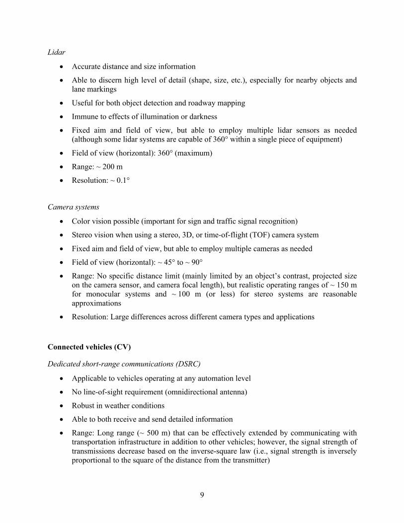
Lidar

• Accurate distance and size information

• Able to discern high level of detail (shape, size, etc.), especially for nearby objects and lane markings

• Useful for both object detection and roadway mapping

• Immune to effects of illumination or darkness

• Fixed aim and field of view, but able to employ multiple lidar sensors as needed (although some lidar systems are capable of 360° within a single piece of equipment)

• Field of view (horizontal): 360° (maximum)

• Range: ~ 200 m

• Resolution: ~ 0.1°

Camera systems

• Color vision possible (important for sign and traffic signal recognition)

• Stereo vision when using a stereo, 3D, or time-of-flight (TOF) camera system

• Fixed aim and field of view, but able to employ multiple cameras as needed

• Field of view (horizontal): ~ 45° to ~ 90°

• Range: No specific distance limit (mainly limited by an object’s contrast, projected size on the camera sensor, and camera focal length), but realistic operating ranges of ~ 150 m for monocular systems and ~ 100 m (or less) for stereo systems are reasonable approximations

• Resolution: Large differences across different camera types and applications

Connected vehicles (CV)

Dedicated short-range communications (DSRC)

• Applicable to vehicles operating at any automation level

• No line-of-sight requirement (omnidirectional antenna)

• Robust in weather conditions

• Able to both receive and send detailed information

• Range: Long range (~ 500 m) that can be effectively extended by communicating with transportation infrastructure in addition to other vehicles; however, the signal strength of transmissions decrease based on the inverse-square law (i.e., signal strength is inversely proportional to the square of the distance from the transmitter)

10

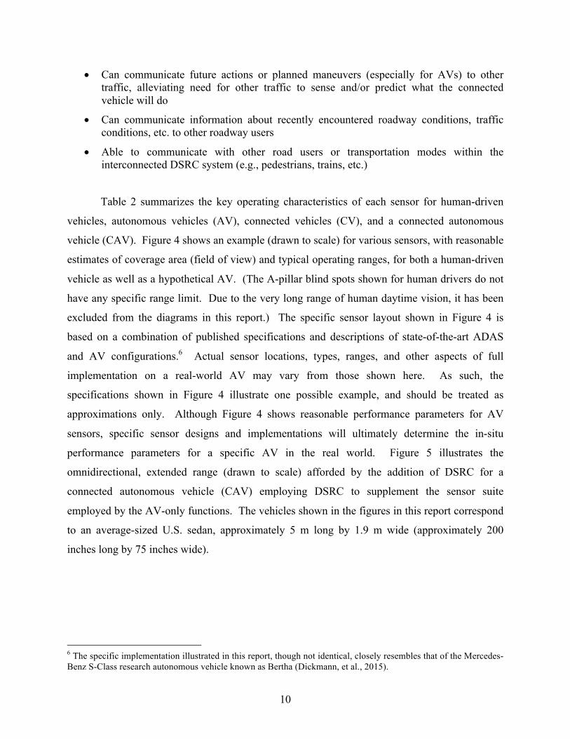
• Can communicate future actions or planned maneuvers (especially for AVs) to other traffic, alleviating need for other traffic to sense and/or predict what the connected vehicle will do

• Can communicate information about recently encountered roadway conditions, traffic conditions, etc. to other roadway users

• Able to communicate with other road users or transportation modes within the interconnected DSRC system (e.g., pedestrians, trains, etc.)

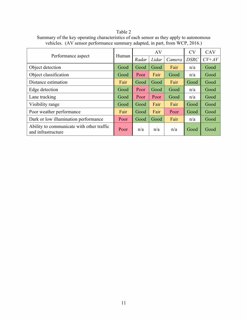
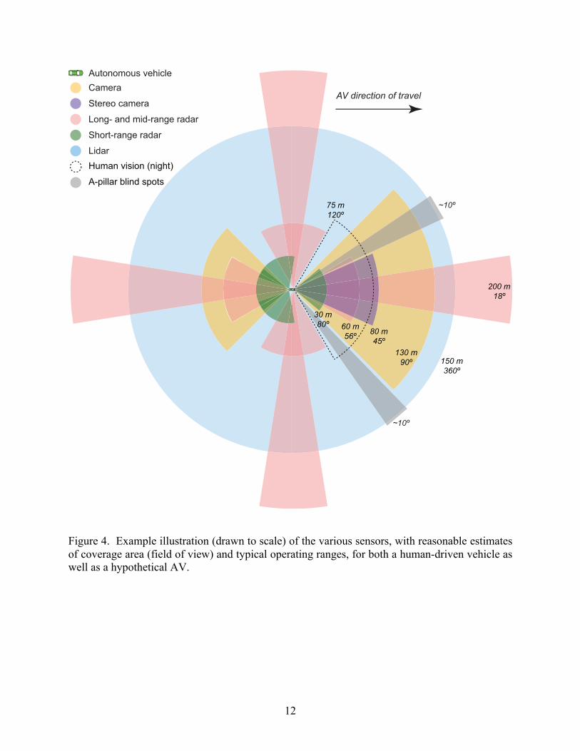
Table 2 summarizes the key operating characteristics of each sensor for human-driven

vehicles, autonomous vehicles (AV), connected vehicles (CV), and a connected autonomous

vehicle (CAV). Figure 4 shows an example (drawn to scale) for various sensors, with reasonable

estimates of coverage area (field of view) and typical operating ranges, for both a human-driven

vehicle as well as a hypothetical AV. (The A-pillar blind spots shown for human drivers do not

have any specific range limit. Due to the very long range of human daytime vision, it has been

excluded from the diagrams in this report.) The specific sensor layout shown in Figure 4 is

based on a combination of published specifications and descriptions of state-of-the-art ADAS

and AV configurations.6 Actual sensor locations, types, ranges, and other aspects of full

implementation on a real-world AV may vary from those shown here. As such, the

specifications shown in Figure 4 illustrate one possible example, and should be treated as

approximations only. Although Figure 4 shows reasonable performance parameters for AV

sensors, specific sensor designs and implementations will ultimately determine the in-situ

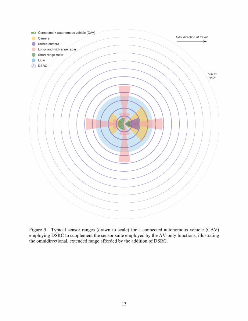
performance parameters for a specific AV in the real world. Figure 5 illustrates the

omnidirectional, extended range (drawn to scale) afforded by the addition of DSRC for a

connected autonomous vehicle (CAV) employing DSRC to supplement the sensor suite

employed by the AV-only functions. The vehicles shown in the figures in this report correspond

to an average-sized U.S. sedan, approximately 5 m long by 1.9 m wide (approximately 200

inches long by 75 inches wide).

6 The specific implementation illustrated in this report, though not identical, closely resembles that of the Mercedes-Benz S-Class research autonomous vehicle known as Bertha (Dickmann, et al., 2015).

11

Table 2 Summary of the key operating characteristics of each sensor as they apply to autonomous

vehicles. (AV sensor performance summary adapted, in part, from WCP, 2016.)

Performance aspect Human AV CV CAV

Radar Lidar Camera DSRC CV+AV Object detection Good Good Good Fair n/a Good Object classification Good Poor Fair Good n/a Good Distance estimation Fair Good Good Fair Good Good Edge detection Good Poor Good Good n/a Good Lane tracking Good Poor Poor Good n/a Good Visibility range Good Good Fair Fair Good Good Poor weather performance Fair Good Fair Poor Good Good Dark or low illumination performance Poor Good Good Fair n/a Good Ability to communicate with other traffic and infrastructure Poor n/a n/a n/a Good Good

12

Figure 4. Example illustration (drawn to scale) of the various sensors, with reasonable estimates of coverage area (field of view) and typical operating ranges, for both a human-driven vehicle as well as a hypothetical AV.

~10º

~10º

200 m18º

150 m360º

130 m90º

80 m45º

60 m56º

30 m80º

75 m120º

Autonomous vehicleCamera

Stereo camera

Long- and mid-range radar

Short-range radar

LidarHuman vision (night)

A-pillar blind spots

AV direction of travel

13

Figure 5. Typical sensor ranges (drawn to scale) for a connected autonomous vehicle (CAV) employing DSRC to supplement the sensor suite employed by the AV-only functions, illustrating the omnidirectional, extended range afforded by the addition of DSRC.

Camera

Stereo camera

Lidar

Short-range radar

Long- and mid-range radar

Connected + autonomous vehicle (CAV)

DSRC

CAV direction of travel

500 m360º

14

Illustrative case studies

Assumptions

The following case studies present a variety of scenarios and vehicle maneuvers, and all

analyses and calculations assume ideal conditions unless otherwise described. The ideal

conditions assumed are as follows:

• All vehicles and tires are in proper working order.

• The human driver is alert and rested, skilled/experienced, and has good color vision with

good visual acuity (i.e., 20/20).

• Human drivers have clear fields of view and AV sensors are clean and functioning

properly. This includes having an unobstructed line of sight (if needed) when discussing

detection distances.

• Both the human driver and AV system will make the appropriate decision for the given

scenario.

• Both the human driver and AV system will be capable of controlling the vehicle when

performing the required maneuver.

• The analyses to follow will discuss performance capabilities of humans and automated

vehicles, but not the associated probabilities of each level of performance occurring.

Minimum stopping distance

The minimum stopping distance for a vehicle is dependent upon the reaction time of the

driver (human or automated), the speed of the vehicle, and the minimum braking distance for

that specific vehicle under the current roadway conditions (e.g., dry, wet, snowy, etc.). For

scenarios involving maximum braking (to achieve the minimum braking distance), the main

variable in the minimum stopping distance for each driver type is reaction time.

Calculations of minimum stopping distances were performed for four scenarios involving

two extreme roadway conditions (dry and wet) and two driver types (human drivers and

automated vehicles operating at level 2 or higher). For each set of roadway conditions and driver

15

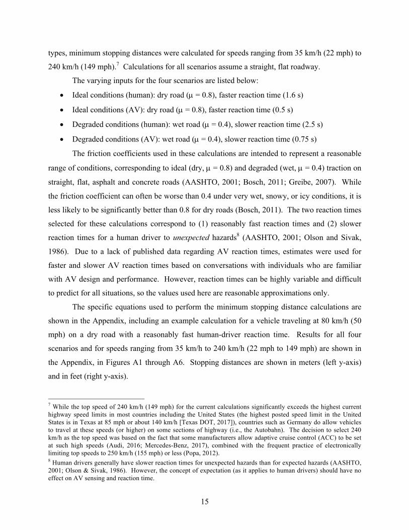
types, minimum stopping distances were calculated for speeds ranging from 35 km/h (22 mph) to

240 km/h (149 mph).7 Calculations for all scenarios assume a straight, flat roadway.

The varying inputs for the four scenarios are listed below:

• Ideal conditions (human): dry road (µ = 0.8), faster reaction time (1.6 s)

• Ideal conditions (AV): dry road (µ = 0.8), faster reaction time (0.5 s)

• Degraded conditions (human): wet road (µ = 0.4), slower reaction time (2.5 s)

• Degraded conditions (AV): wet road (µ = 0.4), slower reaction time (0.75 s)

The friction coefficients used in these calculations are intended to represent a reasonable

range of conditions, corresponding to ideal (dry, µ = 0.8) and degraded (wet, µ = 0.4) traction on

straight, flat, asphalt and concrete roads (AASHTO, 2001; Bosch, 2011; Greibe, 2007). While

the friction coefficient can often be worse than 0.4 under very wet, snowy, or icy conditions, it is

less likely to be significantly better than 0.8 for dry roads (Bosch, 2011). The two reaction times

selected for these calculations correspond to (1) reasonably fast reaction times and (2) slower

reaction times for a human driver to unexpected hazards8 (AASHTO, 2001; Olson and Sivak,

1986). Due to a lack of published data regarding AV reaction times, estimates were used for

faster and slower AV reaction times based on conversations with individuals who are familiar

with AV design and performance. However, reaction times can be highly variable and difficult

to predict for all situations, so the values used here are reasonable approximations only.

The specific equations used to perform the minimum stopping distance calculations are

shown in the Appendix, including an example calculation for a vehicle traveling at 80 km/h (50

mph) on a dry road with a reasonably fast human-driver reaction time. Results for all four

scenarios and for speeds ranging from 35 km/h to 240 km/h (22 mph to 149 mph) are shown in

the Appendix, in Figures A1 through A6. Stopping distances are shown in meters (left y-axis)

and in feet (right y-axis).

7 While the top speed of 240 km/h (149 mph) for the current calculations significantly exceeds the highest current highway speed limits in most countries including the United States (the highest posted speed limit in the United States is in Texas at 85 mph or about 140 km/h [Texas DOT, 2017]), countries such as Germany do allow vehicles to travel at these speeds (or higher) on some sections of highway (i.e., the Autobahn). The decision to select 240 km/h as the top speed was based on the fact that some manufacturers allow adaptive cruise control (ACC) to be set at such high speeds (Audi, 2016; Mercedes-Benz, 2017), combined with the frequent practice of electronically limiting top speeds to 250 km/h (155 mph) or less (Popa, 2012). 8 Human drivers generally have slower reaction times for unexpected hazards than for expected hazards (AASHTO, 2001; Olson & Sivak, 1986). However, the concept of expectation (as it applies to human drivers) should have no effect on AV sensing and reaction time.

16

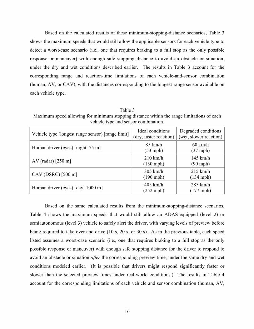
Based on the calculated results of these minimum-stopping-distance scenarios, Table 3

shows the maximum speeds that would still allow the applicable sensors for each vehicle type to

detect a worst-case scenario (i.e., one that requires braking to a full stop as the only possible

response or maneuver) with enough safe stopping distance to avoid an obstacle or situation,

under the dry and wet conditions described earlier. The results in Table 3 account for the

corresponding range and reaction-time limitations of each vehicle-and-sensor combination

(human, AV, or CAV), with the distances corresponding to the longest-range sensor available on

each vehicle type.

Table 3 Maximum speed allowing for minimum stopping distance within the range limitations of each

vehicle type and sensor combination.

Vehicle type (longest range sensor) [range limit] Ideal conditions (dry, faster reaction)

Degraded conditions (wet, slower reaction)

Human driver (eyes) [night: 75 m] 85 km/h (53 mph)

60 km/h (37 mph)

AV (radar) [250 m] 210 km/h (130 mph)

145 km/h (90 mph)

CAV (DSRC) [500 m] 305 km/h (190 mph)

215 km/h (134 mph)

Human driver (eyes) [day: 1000 m] 405 km/h (252 mph)

285 km/h (177 mph)

Based on the same calculated results from the minimum-stopping-distance scenarios,

Table 4 shows the maximum speeds that would still allow an ADAS-equipped (level 2) or

semiautonomous (level 3) vehicle to safely alert the driver, with varying levels of preview before

being required to take over and drive (10 s, 20 s, or 30 s). As in the previous table, each speed

listed assumes a worst-case scenario (i.e., one that requires braking to a full stop as the only

possible response or maneuver) with enough safe stopping distance for the driver to respond to

avoid an obstacle or situation after the corresponding preview time, under the same dry and wet

conditions modeled earlier. (It is possible that drivers might respond significantly faster or

slower than the selected preview times under real-world conditions.) The results in Table 4

account for the corresponding limitations of each vehicle and sensor combination (human, AV,

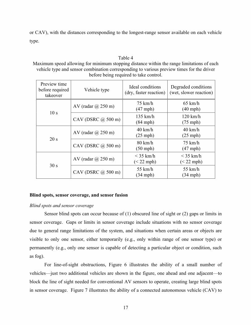
17

or CAV), with the distances corresponding to the longest-range sensor available on each vehicle

type.

Table 4 Maximum speed allowing for minimum stopping distance within the range limitations of each

vehicle type and sensor combination corresponding to various preview times for the driver before being required to take control.

Preview time before required

takeover Vehicle type Ideal conditions

(dry, faster reaction) Degraded conditions (wet, slower reaction)

10 s AV (radar @ 250 m) 75 km/h

(47 mph) 65 km/h (40 mph)

CAV (DSRC @ 500 m) 135 km/h (84 mph)

120 km/h (75 mph)

20 s AV (radar @ 250 m) 40 km/h

(25 mph) 40 km/h (25 mph)

CAV (DSRC @ 500 m) 80 km/h (50 mph)

75 km/h (47 mph)

30 s AV (radar @ 250 m) < 35 km/h

(< 22 mph) < 35 km/h (< 22 mph)

CAV (DSRC @ 500 m) 55 km/h (34 mph)

55 km/h (34 mph)

Blind spots, sensor coverage, and sensor fusion

Blind spots and sensor coverage

Sensor blind spots can occur because of (1) obscured line of sight or (2) gaps or limits in

sensor coverage. Gaps or limits in sensor coverage include situations with no sensor coverage

due to general range limitations of the system, and situations when certain areas or objects are

visible to only one sensor, either temporarily (e.g., only within range of one sensor type) or

permanently (e.g., only one sensor is capable of detecting a particular object or condition, such

as fog).

For line-of-sight obstructions, Figure 6 illustrates the ability of a small number of

vehicles—just two additional vehicles are shown in the figure, one ahead and one adjacent—to

block the line of sight needed for conventional AV sensors to operate, creating large blind spots

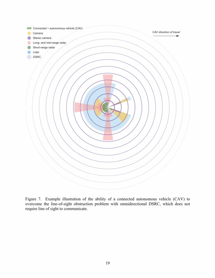
in sensor coverage. Figure 7 illustrates the ability of a connected autonomous vehicle (CAV) to

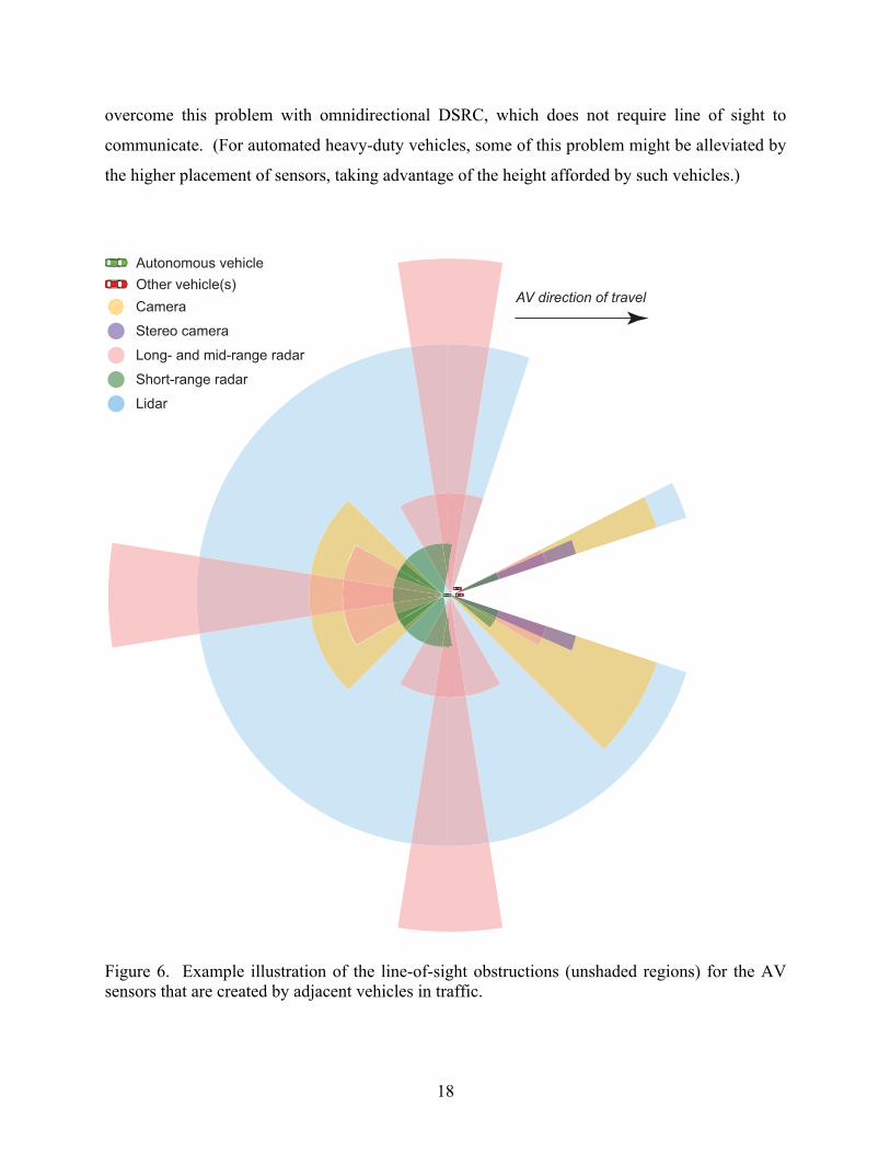
18

overcome this problem with omnidirectional DSRC, which does not require line of sight to

communicate. (For automated heavy-duty vehicles, some of this problem might be alleviated by

the higher placement of sensors, taking advantage of the height afforded by such vehicles.)

Figure 6. Example illustration of the line-of-sight obstructions (unshaded regions) for the AV sensors that are created by adjacent vehicles in traffic.

Camera

Stereo camera

Lidar

Short-range radar

Long- and mid-range radar

Autonomous vehicleOther vehicle(s)

AV direction of travel

19

Figure 7. Example illustration of the ability of a connected autonomous vehicle (CAV) to overcome the line-of-sight obstruction problem with omnidirectional DSRC, which does not require line of sight to communicate.

Camera

Stereo camera

Lidar

Short-range radar

Long- and mid-range radar

Connected + autonomous vehicle (CAV)

DSRC

CAV direction of travel

20

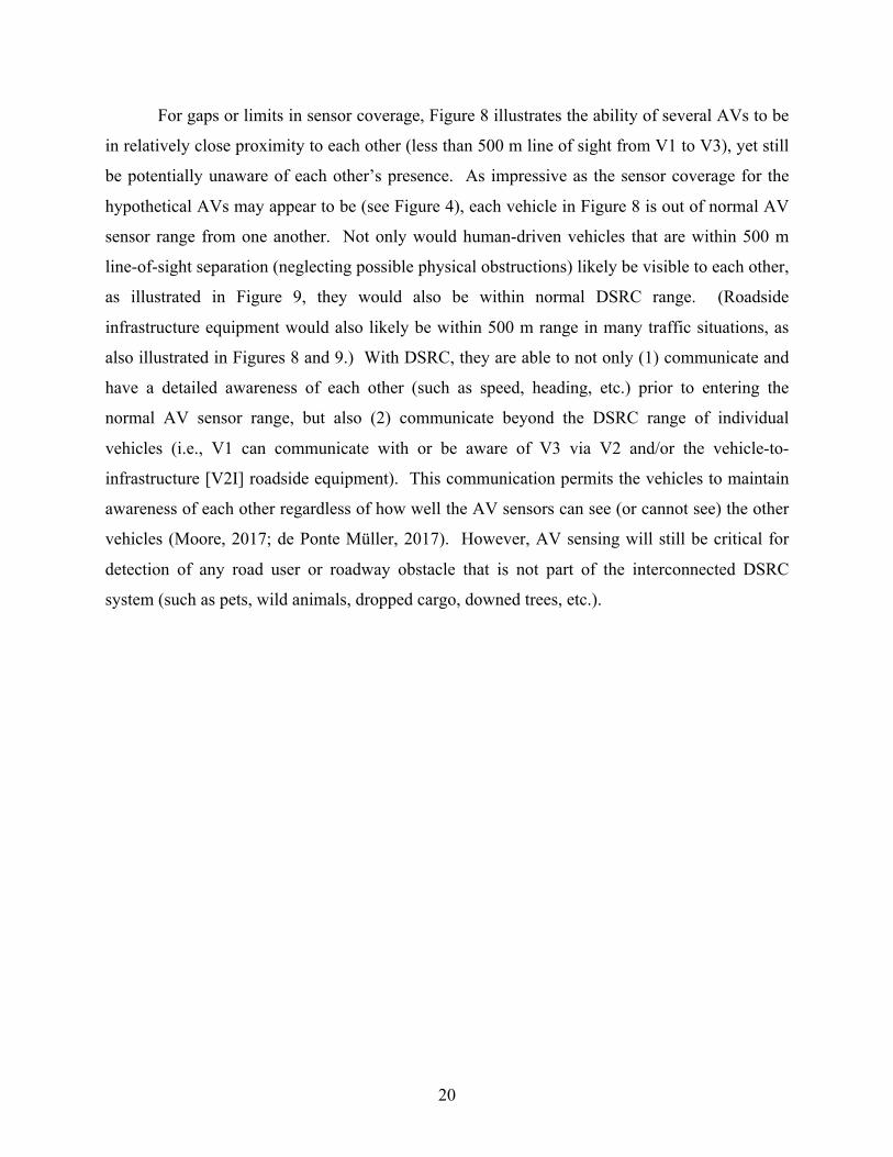
For gaps or limits in sensor coverage, Figure 8 illustrates the ability of several AVs to be

in relatively close proximity to each other (less than 500 m line of sight from V1 to V3), yet still

be potentially unaware of each other’s presence. As impressive as the sensor coverage for the

hypothetical AVs may appear to be (see Figure 4), each vehicle in Figure 8 is out of normal AV

sensor range from one another. Not only would human-driven vehicles that are within 500 m

line-of-sight separation (neglecting possible physical obstructions) likely be visible to each other,

as illustrated in Figure 9, they would also be within normal DSRC range. (Roadside

infrastructure equipment would also likely be within 500 m range in many traffic situations, as

also illustrated in Figures 8 and 9.) With DSRC, they are able to not only (1) communicate and

have a detailed awareness of each other (such as speed, heading, etc.) prior to entering the

normal AV sensor range, but also (2) communicate beyond the DSRC range of individual

vehicles (i.e., V1 can communicate with or be aware of V3 via V2 and/or the vehicle-to-

infrastructure [V2I] roadside equipment). This communication permits the vehicles to maintain

awareness of each other regardless of how well the AV sensors can see (or cannot see) the other

vehicles (Moore, 2017; de Ponte Müller, 2017). However, AV sensing will still be critical for

detection of any road user or roadway obstacle that is not part of the interconnected DSRC

system (such as pets, wild animals, dropped cargo, downed trees, etc.).

21

Figure 8. Example illustration of the ability of several AVs to be in relatively close proximity to each other (less than 500 m line of sight from V1 to V3), yet still be out of normal AV sensor range and potentially unaware of each other’s presence. (Sensor ranges are the same as those shown in Figure 4.)

Camera

Stereo camera

Lidar

Short-range radar

Long- and mid-range radar

Autonomous vehicle (AV)

V1

V2 V3

Roadsideinfrastructure

(V2I)

Scale: 100 m 200 m 300 m

22

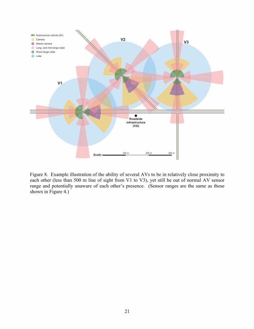
Figure 9. Example illustration of the overlapping DSRC ranges for each vehicle and the roadside infrastructure (V2I) equipment, allowing for detailed awareness of each vehicle (such as speed, heading, etc.) prior to entering the normal AV sensor ranges. (Sensor ranges are the same as those shown in Figure 4.)

V1

V2 V3Camera

Stereo camera

Lidar

Short-range radar

Long- and mid-range radar

Connected + autonomous vehicle (CAV)

DSRC

Roadsideinfrastructure

(V2I)

23

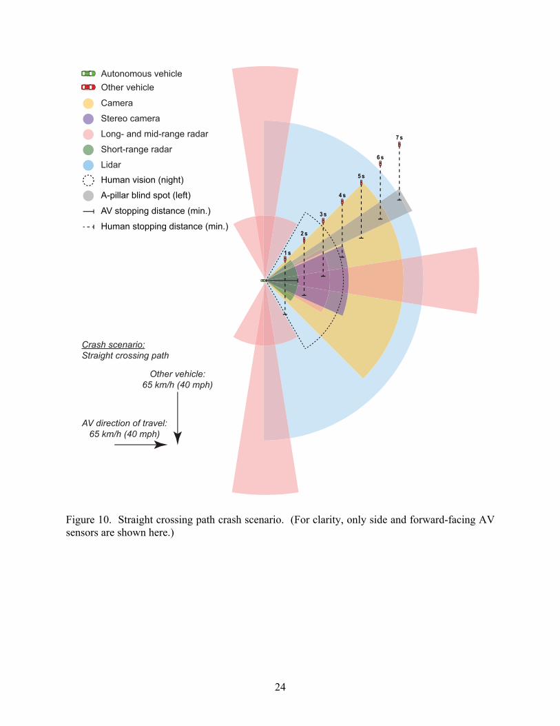
Straight crossing path crashes Other vehicles can travel through large blind spots or gaps in sensors, or potentially

through zones where only one sensor is able to see the vehicle, or even skirt the edge of where

two sensors overlap, creating a possible tracking problem as that vehicle repeatedly enters then

leaves the field of view for a particular sensor. Each of these scenarios can result in minimal or

possibly no coverage, or late coverage (in terms of safe reaction time). An example illustrating a

similar overall layout and geometry to a documented Google AV crash that occurred on

September 23, 2016, in Mountain View, California (California DMV, 2016) is shown in

Figure 10. The exact geometry and speeds for the referenced crash are not identical to the

simplified scenario shown here. Therefore, this discussion of an example crash scenario is not

intended as an analysis of the specific referenced crash. However, the example scenario was

selected because a similar scenario had proven to be problematic for a highly automated vehicle

(level 3) in the real world. In the scenario illustrated here, two potential problems exist: the other

vehicle is either (1) visible to only one sensor (i.e., lidar), or (2) it skirts the edge of a sensor’s

range (i.e., camera).

Assuming unobstructed line of sight for both human drivers and AV sensors, the other

vehicle would have been visible to a human driver for the entire 7 s (or more) prior to a collision

during both day or night (the approaching vehicle would be assumed to also have headlamps

illuminated, negating the 75 m limit for nighttime vision). The other vehicle would have entered

the range of the lidar sensor with just under 6 s to collision, possibly entering camera range

around 5 s before collision (but possibly also remaining just outside of camera range).

With a human-driven vehicle needing a distance corresponding to just under 3 s of travel

to stop at 65 km/h (40 mph), a human driver would have a buffer of 4 s (or more) to react and

stop. (Stopping distances assume a dry road with a faster reaction time.) The AV needs a

distance corresponding to just over 1.5 s of travel to stop at 65 km/h (40 mph), and would have a

buffer of around 4 s (but not likely more) to react and stop during both day or night (most

sensors are not affected by darkness or illumination levels). In this example scenario, the AV

has approximately the same amount of time (or less) to respond as the human driver. Significant

improvement in the time available for an AV to respond would require (1) increased sensor

range, (2) increased sensor coverage, and/or (3) faster AV reaction time.

24

Figure 10. Straight crossing path crash scenario. (For clarity, only side and forward-facing AV sensors are shown here.)

Camera

Stereo camera

Lidar

Short-range radar

Long- and mid-range radar

Human vision (night)

A-pillar blind spot (left)

Autonomous vehicleOther vehicle

AV stopping distance (min.)

Human stopping distance (min.)

6 s

5 s

4 s

3 s

2 s

1 s

7 s

Crash scenario:Straight crossing path

AV direction of travel:65 km/h (40 mph)

Other vehicle:65 km/h (40 mph)

25

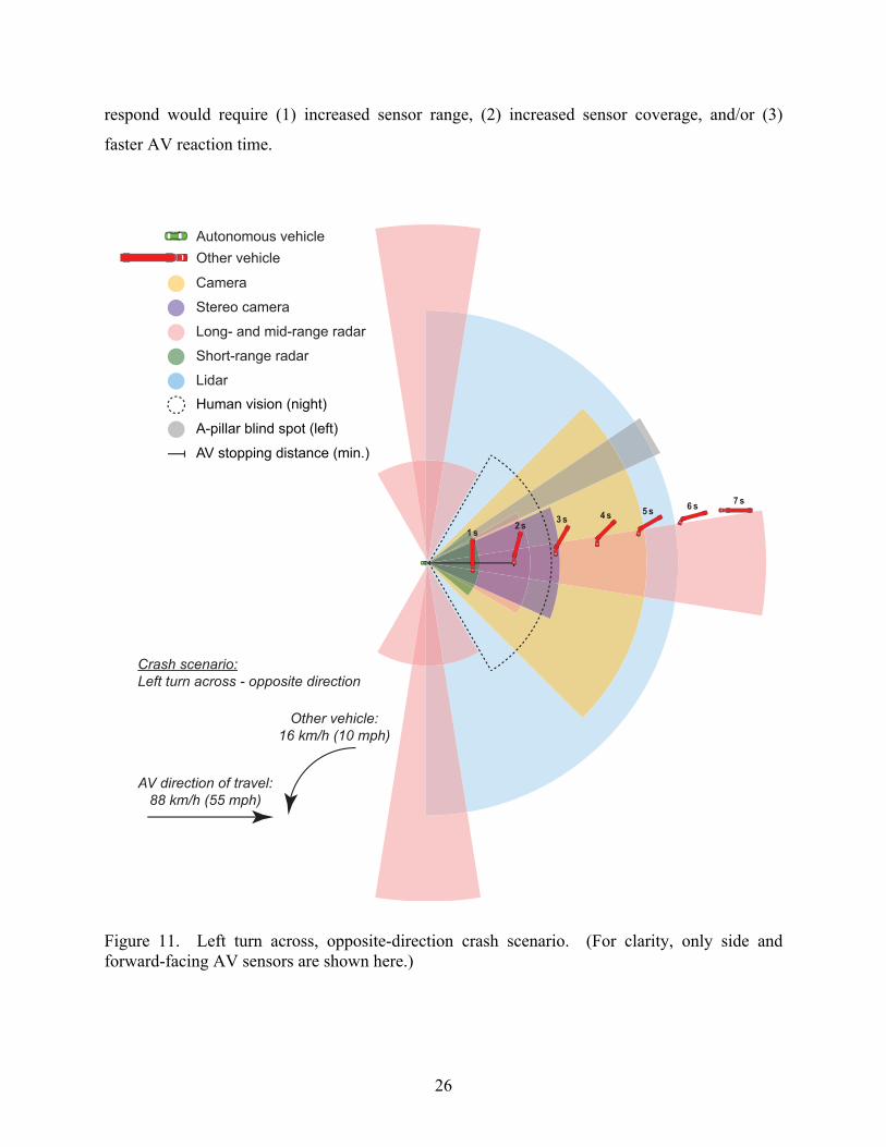
Left turn across, opposite-direction crashes Similar to the straight crossing path example, other vehicles can travel through zones

where only one sensor is able to see the vehicle, or skirting the edge where two sensors overlap,

creating a tracking problem as that vehicle enters then leaves the field of view in rapid

succession for a particular sensor. The other vehicle might be seen as parallel, non-crossing

traffic until very late (in terms of safe reaction time), prior to turning/crossing. An example

illustrating a similar overall layout and geometry to the well-publicized Tesla crash that occurred

on May 7, 2016, in Williston, Florida (NHTSA, 2017b) is shown in Figure 11. The exact

geometry and speeds for the referenced crash are not identical to the simplified scenario shown

here. Therefore, this discussion of an example crash scenario is not intended as an analysis of

the specific referenced crash. However, the example scenario was selected because a similar

scenario had proven to be problematic for a highly automated vehicle (level 2) in the real world.

In the scenario illustrated here, the other vehicle (1) enters the sensor coverage area relatively

late (less than 6 s to collision), and (2) skirts the edge of a sensor’s range (i.e., long-range radar).

Assuming unobstructed line of sight for both human drivers and AV sensors, and

assuming the other vehicle started to turn between 7 s and 6 s to collision, the other vehicle

would have been visible to a human driver for the entire 7 s (or more) prior to a collision during

both day or night (the approaching vehicle would be assumed to also have headlamps

illuminated, negating the 75 m limit for nighttime vision). The other vehicle would have entered

the range of the lidar sensor with just under 6 s to collision, then entered the coverage area of the

camera and long-range radar at around 5 s, then stereo camera range at around 3 s, and short-

range radar just before 2 s. (Detection that occurs after that time would be too late to stop the

vehicle and avoid a collision.)

With a human-driven vehicle needing a distance corresponding to just over 3 s of travel

to stop at 88 km/h (55 mph), a human driver would have a buffer of between 3 s and 4 s to react

and stop. (Stopping distances assume a dry road with a faster reaction time.) The AV needs a

distance corresponding to just over 2 s of travel to stop at 88 km/h (55 mph), and would have a

buffer of around 4 s to react and stop during both day or night (most sensors are not affected by

darkness or illumination levels). In this example scenario, the AV has approximately 1 s more

than the human driver to respond. Significant improvement in the time available for an AV to

26

respond would require (1) increased sensor range, (2) increased sensor coverage, and/or (3)

faster AV reaction time.

Figure 11. Left turn across, opposite-direction crash scenario. (For clarity, only side and forward-facing AV sensors are shown here.)

Camera

Stereo camera

Lidar

Short-range radar

Long- and mid-range radar

Human vision (night)

A-pillar blind spot (left)

Autonomous vehicleOther vehicle

AV stopping distance (min.)

7 s6 s5 s4 s3 s2 s1 s

Crash scenario:Left turn across - opposite direction

AV direction of travel:88 km/h (55 mph)

Other vehicle:16 km/h (10 mph)

27

Sensor fusion The selected case studies illustrated in this report show that some traffic scenarios still

pose a challenge for automated vehicles. The two specific crash geometries described in the

previous subsections (both considered angle-impact crashes) were also identified by NHTSA as

being especially problematic for automated vehicles.9 The likelihood or probability that an AV

will react to a hazard (based on processing and perception) is a separate issue from theoretically

available time to react (based on sensor range or technical capabilities). In a recent report

investigating crash-imminent braking (CIB) systems (i.e., automated braking), NHTSA found

that for four specific scenarios, including straight crossing path and left turn across, opposite

direction crashes, “system performance, regardless of system configuration or settings, [was] not

capable of reliably responding” (NHTSA, 2011a). In agreement with both crash scenarios

presented in this report, the NHTSA report states that, “the limited time the target is in the field

of view prior to impact challenges the system’s ability to perform threat assessment and apply

the CIB system. A target is usually recognized very late or not at all prior to impact” (NHTSA,

2011b). (These same findings were also quoted in the NHTSA investigative report for the Tesla

crash referenced earlier in this report [NHTSA, 2017b].)10

However, such systems rely predominantly on radar and single cameras, and the potential

to improve performance in these scenarios is considerably better when additional,

complementary sensors such as lidar and stereo camera systems are all brought together to

analyze the roadway and environment. This is particularly true when the sensor-fusion strategy

of a system requires at least two sensors to agree before taking action (usually to avoid false

activation) (Dickmann, et al., 2015). However, waiting for such sensor agreement can be

problematic, especially when “complex or unusual shapes may delay or prevent the system from

classifying certain vehicles as targets/threats” (NHTSA, 2017b). Ultimately, to maximize

performance and available response time beyond the range of typical AV sensors, it is crucial to

9 It should be noted that these types of crashes are also problematic for human drivers, with 6,446 fatalities occurring in angle-impact crashes, contributing to around 18% of the 35,092 fatalities on U.S. roadways in 2015 (NHTSA, 2017a). 10 While the CIB tests referenced by NHTSA were performed in 2011, no significant improvements in CIB performance for these types of crashes appear to have occurred since that report. The NHTSA (2017b) investigative report for the Tesla crash states that, “ODI surveyed a dozen automotive manufacturers and several major suppliers to determine if the AEB capabilities in crossing path collisions had changed since the CAMP CIB project was completed. None of the companies contacted by ODI indicated that AEB systems used in their products through MY 2016 production were designed to brake for crossing path collisions.”

28

effectively fuse sensor input and data acquisition across all forms, integrating traditional AV

technologies with connected-vehicle technologies (DSRC) for a complete CAV. If the vehicles

in the previous crash examples were all connected vehicles (autonomous or human driven), they

would have been well within DSRC range for the 7 s prior to a potential crash shown in each

diagram. Implementation of omnidirectional DSRC satisfies the need for both (1) extended

range and (2) extended coverage area identified in the two previous example crash scenarios.

29

Other useful sensors not discussed in this report There are several other potentially useful sensors that might be considered for use with

automated vehicles. The following list, though not exhaustive, identifies some of the most

common additional sensors not discussed in this report, and their related capabilities:

• Far-infrared (heat; 50-1000 µm) sensor: Often used for night-vision systems for human

drivers, far-infrared sensors are capable of passively detecting heat differences in the

environment, which is particularly useful for detecting humans and animals present in the

roadway.

• Mid- and near-infrared sensors: Capable of projecting and receiving middle (3-50 µm)

and near (0.75-3 µm) infrared (IR) wavelengths, which allows these devices to illuminate

their environment with an invisible (and potentially high power) IR source.

• Dead reckoning sensors and/or inertial measurement units (IMU): accelerometers,

gyroscopes, and/or magnetometers in IMU; chassis control sensors in locations such as

wheels, brakes, steering, etc. Used for both electronic stability-control systems and also

potentially for vehicle navigation.

• Tire-based sensors: capable of detecting and communicating data about the current

physical condition of each tire, specifications and manufacturing information, and/or

current roadway conditions.

While the addition of the sensors listed here (or others) would extend the effectiveness of

an AV’s sensing capabilities, each additional sensor type would also add to the overall

processing load for the self-driving system to properly interpret and respond to sensor inputs.

30

Key findings This white paper analyzed and compared the sensing capabilities of human drivers and

highly automated vehicles. The key findings from this study are as follows:

• Machines/computers are generally well suited to perform tasks like driving,

especially in regard to reaction time (speed), power output and control, consistency

(especially for tasks requiring constant vigilance), and multichannel information

processing.

• At slow speeds, AV performance under degraded conditions may actually exceed

human-driver performance under ideal conditions.

• Human drivers still generally maintain an advantage in terms of reasoning,

perception, and sensing when driving.

• Matching (or exceeding) human sensing capabilities requires AVs to employ a variety

of sensors, which in turn requires complete sensor fusion across the system, combining

all sensor inputs to form a unified view of the surrounding roadway and environment.

• While no single sensor completely equals human sensing capabilities, some offer

capabilities not possible for a human driver (e.g., accurate distance measurement with

lidar, seeing through inclement weather with radar).

• Integration of connected-vehicle (CV) technology (e.g., DSRC) extends the effective

range and coverage area of both human-driven vehicles and AVs, with a longer operating

range and omnidirectional communication that does not require unobstructed line of sight

the way human drivers and AVs generally do.

• Combining human-driven vehicles or AVs that can “see” traffic and their

environment with CVs that can “talk” to other traffic and their environment maximizes

potential awareness of other roadway users and roadway conditions.

• AV sensing will still be critical for detection of any road user or roadway obstacle

that is not part of the interconnected DSRC system (such as pets, wild animals, dropped

cargo, downed trees, etc.)

• A fully implemented connected autonomous vehicle (CAV) offers the best potential

to effectively and safely replace the human driver when operating vehicles at automation

levels 4 and 5.

31

References AASHTO [American Association of State Highway and Transportation Officials]. (2001). A

policy on geometric design of highways and streets. Available at: https://nacto.org/docs/usdg/geometric_design_highways_and_streets_aashto.pdf

Anthony, S. E. (2016, March 1). The trollable self-driving car. Available at: http://www.slate.com/articles/technology/future_tense/2016/03/google_self_driving_cars_lack_a_human_s_intuition_for_what_other_drivers.html

Audi. (2016). Adaptive cruise control with stop & go function. Available at: https://www.audi-technology-portal.de/en/electrics-electronics/driver-assistant-systems/adaptive-cruise-control-with-stop-go-function

Bhise, V. D. (2012). Ergonomics in the automotive design process. Boca Raton, FL: Taylor & Francis Group, LLC. Available at: https://doi.org/10.1201/b11237

Bosch. (2009). Chassis systems control. LRR3: 3rd generation long-range radar sensor. Available at: http://products.bosch-mobility-solutions.com/media/db_application/downloads/pdf/safety_1/en_4/lrr3_datenblatt_de_2009.pdf

Bosch. (2011). Automotive handbook. 8th ed., rev. and extended. Plochingen, Germany: Robert Bosch.

Boyce, P. R. (2014). Human factors in lighting, third edition. Boca Raton, FL: Taylor & Francis Group, LLC. Available at: https://doi.org/10.1201/b16707

Burress, B. (2007). The unaided eye. Available at: https://ww2.kqed.org/quest/2007/09/28/the-unaided-eye/

California DMV [California Department of Motor Vehicles]. (2016). Report of traffic accident involving an autonomous vehicle (OL 316); Google September 23, 2016. Available at: https://www.dmv.ca.gov/portal/wcm/connect/d3f31000-2d71-4483-9584-70be2f2ed2c5/google_092316.pdf?MOD=AJPERES

CAPTCHA [Completely Automated Public Turing test to tell Computers and Humans Apart]. (2017). CAPTCHA: Telling humans and computers apart automatically. Available at: http://www.captcha.net/

Continental. (2017). Long range radar. Available at: http://www.continental-automated-driving.com/Navigation/Enablers/Radar/Long-Range-Radar

Cummings, M. (2014). Man versus machine or man + machine? IEEE Intelligent Systems, 29(5), 62-69. Available at: http://ieeexplore.ieee.org/document/6949509/

CVEL [Clemson Vehicular Electronics Laboratory]. (2017). Automotive electronic systems. Available at: http://www.cvel.clemson.edu/auto/systems/auto-systems.html

32

Daimler. (2014). World premiere for the traffic system of tomorrow – more efficient, safer, networked – and autonomous. Available at: http://media.daimler.com/marsMediaSite/ko/en/9905075

Daimler. (2017a). The auto pilot for trucks. Available at: https://www.daimler.com/innovation/autonomous-driving/special/technology-trucks.html

Daimler. (2017b). The Mercedes-Benz future bus. Available at: https://www.daimler.com/innovation/autonomous-driving/future-bus.html

Dickmann, J., Appenrodt, N., Klappstein, J., Bloecher, H.-L., Muntzinger, M., Sailer, A., Hahn, M., & Brenk, C. (2015). Making Bertha see even more: Radar contribution. IEEE Access, 3, 1233-1247. Available at: http://ieeexplore.ieee.org/document/7161279/

Falson, A. (2014, November 19). Mercedes-Benz steps up autonomous vehicle technology. Available at: http://performancedrive.com.au/mercedes-benz-steps-autonomous-vehicle-technology-1913/

Fitts, P. M. (Ed.). (1951). Human engineering for an effective air-navigation and traffic-control system. Washington, D.C.: National Research Council.

Fitts, P. M. (1962). Functions of man in complex systems. Aerospace Engineering, 21, 34-39.

FMCSA [Federal Motor Carrier Safety Administration]. (2017). Large truck and bus crash facts 2015. Available at: https://www.fmcsa.dot.gov/safety/data-and-statistics/large-truck-and-bus-crash-facts-2015#A3

Ford. (2017). Further with Ford. Available at: https://media.ford.com/content/fordmedia/fna/us/en/news/2016/09/12/further-with-ford.html

Freedman, D. H. (2017). Self-driving trucks. Available at: https://www.technologyreview.com/s/603493/10-breakthrough-technologies-2017-self-driving-trucks/

Godsmark, P. (2017, February 24). Driverless, autonomous, self-driving… naming a baby is easier than naming new car tech. https://www.driverless.id/news/driverless-autonomous-self-driving-naming-baby-is-easier-than-naming-new-car-tech-0175495/

Google (2015). Google self-driving car project monthly report, July 2015. Available at: https://www.google.com/selfdrivingcar/files/reports/report-0715.pdf

Greibe, P. (2007). Braking distance, friction and behaviour. Available at: http://www.trafitec.dk/sites/default/files/publications/braking%20distance%20-%20friction%20and%20driver%20behaviour.pdf

Hammerschmidt, C. (2013, September 11). Daimler, KIT send autonomous vehicle on historic course. Available at: http://www.eenewsautomotive.com/news/daimler-kit-send-autonomous-vehicle-historic-course

33

Hyundai. (2016). Hyundai motor company introduces new autonomous Ioniq concept at Automobility Los Angeles. Available at: https://www.hyundaiusa.com/about-hyundai/news/corporate_hyundai-motor-company- introduces-new-autonomous-ioniq-concept-at-automobility-los-angeles4-20161116.aspx

Kenney, J. B. (2011). Dedicated short-range communications (DSRC) standards in the United States. Proceedings of the IEEE, 99(7), 1162-1182. Available at: http://ieeexplore.ieee.org/document/5888501/

Kent, L. (2015). Autonomous cars can only understand the real world through a map. Available at: http://360.here.com/2015/04/16/autonomous-cars-can-understand-real-world-map/

Krok, A. (2016, November 16). Hyundai's next Ioniq is a fully autonomous concept. Available at: https://www.cnet.com/roadshow/news/hyundais-next-ioniq-is-a-fully-autonomous-concept/

LeddarTech. (2016). LeddarTech launches LeddarVu, a new scalable platform towards high-resolution LiDAR. Available at: http://leddartech.com/leddartech-launches-leddarvu-new-scalable-platform-towards-high-resolution-lidar/

Lee, S. & Lim, A. (2013). An empirical study on ad hoc performance of DSRC and Wi-Fi vehicular communications. International Journal of Distributed Sensor Networks, 9(11). Available at: http://journals.sagepub.com/doi/full/10.1155/2013/482695

Lee, Y. M. & Sheppard, E. (2016). The effect of motion and signalling on drivers’ ability to predict intentions of other road users. Accident Analysis and Prevention, 95, 202-208. Available at: http://www.sciencedirect.com/science/article/pii/S0001457516302408

MacAdam, C. C. (2003). Understanding and modeling the human driver. Vehicle System Dynamics, 40(1-3), 101-134. Available at: http://hdl.handle.net/2027.42/65021

McDonald, M. (2015, October 16). Automotive fusion: Combining legacy and emerging sensors for safer and increasingly autonomous vehicles. Available at: http://www.sensorsmag.com/components/automotive-fusion-combining-legacy-and-emerging-sensors-for-safer-and-increasingly

Mercedes-Benz. (2017). Distronic Plus. Available at: https://www.mbusa.com/mercedes/technology/videos/detail/class-CLA_Class/title-claclass/videoId-caf758b451127410VgnVCM100000ccec1e35RCRD

Moore, N. C. (2017, June 23). Mcity demos: Self-driving cars can be even safer with connected technology. Available at: http://ns.umich.edu/new/multimedia/videos/24932-mcity-demos-self-driving-cars-can-be-even-safer-with-connected-technology

34

NHTSA [National Highway Traffic Safety Administration]. (2016). Federal automated vehicles policy. Available at: https://one.nhtsa.gov/nhtsa/av/pdf/Federal_Automated_Vehicles_Policy.pdf

NHTSA [National Highway Traffic Safety Administration]. (2017a). Fatality Analysis Reporting System (FARS) encyclopedia. Available at: http://www-fars.nhtsa.dot.gov/Main/index.aspx

NHTSA [National Highway Traffic Safety Administration]. (2017b). ODI resume. Automatic vehicle control systems. Available at: https://static.nhtsa.gov/odi/inv/2016/INCLA-PE16007-7876.PDF

NHTSA [National Highway Traffic Safety Administration]. (2017c). Vehicle-to-vehicle communications. Available at: https://www.safercar.gov/v2v/index.html

NSC [National Safety Council]. (2017). The most dangerous time to drive. Available at: http://www.nsc.org/learn/safety-knowledge/Pages/news-and-resources-driving-at-night.aspx

Ohnsman, A. (2017, May 14). Waymo forges driverless car tech tie-up with Lyft amid its legal battle with Uber. Available at: https://www.forbes.com/sites/alanohnsman/2017/05/14/waymo-forges-driverless-car-tech-tie-up-with-lyft-amid-its-legal-battle-with-uber/#4486bc126594

Olson, P. L. & Sivak, M. (1986). Perception-response time to unexpected roadway hazards. Human Factors, 28(1), 91-96. Available at: http://journals.sagepub.com/doi/abs/10.1177/001872088602800110

Owsley, C. & McGwin, G., Jr. (2010). Vision and driving. Vision Research, 50(23), 2348-2361.

Pleskot, K. (2016, November 16). Hyundai Ioniq autonomous concept debuts hidden lidar system in L.A. Available at: http://www.motortrend.com/news/hyundai-ioniq-autonomous-concept-debuts-hidden-lidar-system-in-l-a/

de Ponte Müller, F. (2017). Survey on ranging sensors and cooperative techniques for relative positioning of vehicles. Sensors, 17, 271-287. Available at: http://www.mdpi.com/1424-8220/17/2/271

Popa, B. (2012, July 28). Gentlemen’s agreement: Not so fast, sir! Available at: https://www.autoevolution.com/news/gentlemens-agreement-not-so-fast-sir-47736.html

Quanergy. (2015). 360° 3D LIDAR M8-1 sensor. Available at: http://www.lidarusa.com/uploads/5/4/1/5/54154851/quanergy_m8-1_lidar_datasheet_v4.0.pdf

RITA [Research and Innovative Technology Administration]. (2016). Dedicated short-range communications (DSRC). Available at: https://www.its.dot.gov/factsheets/pdf/JPO-034_DSRC.pdf

35

Rosenholtz, R., Li, Y., & Nakano, L. (2007). Measuring visual clutter. Journal of Vision, 7(2), 1-22. Available at: http://jov.arvojournals.org/article.aspx?articleid=2122001

Schoettle, B. & Flannagan, M. J. (2011). A market-weighted description of low-beam and high-beam headlighting patterns in the U.S.: 2011 (Technical Report No. UMTRI-2011-33). Ann Arbor: University of Michigan Transportation Research Institute.

Sivak, M. & Schoettle, B. (2015). Road safety with self-driving vehicles: General limitations and road sharing with conventional vehicles (Technical Report No. UMTRI-2015-2). Available at: http://hdl.handle.net/2027.42/111735

Sivak, M., Schoettle, B., Reed, M. P., & Flannagan, M. J. (2007). Body-pillar vision obstructions and lane-change crashes. Journal of Safety Research, 38, 557-561. Available at: http://www.sciencedirect.com/science/article/pii/S002243750700103X

Sommer, C., Eckhoff, D., & Dressler, F. (2013). IVC in cities: Signal attenuation by buildings and how parked cars can improve the situation. IEEE Transactions on Mobile Computing, 13(8), 1733-1745. Available at: http://ieeexplore.ieee.org/document/6544519/

Texas DOT [Texas Department of Transportation]. (2017). Setting speed limits. Available at: http://www.txdot.gov/driver/laws/speed-limits/setting.html

Utah DOT [Utah Department of Transportation]. (2013). Utah DOT leveraging LiDAR for asset management leap. Available at: http://blog.udot.utah.gov/2013/02/utah-dot-leveraging-lidar-for-asset-management-leap/

Walker, A. (2015, October 12). 5 cities with driverless public buses on the streets right now. Available at: http://gizmodo.com/5-cities-with-driverless-public-buses-on-the-streets-ri-1736146699

de Winter, J. C. F. & Dodou, D. (2014). Why the Fitts list has persisted throughout the history of function allocation. Cognition, Technology & Work, 16(1), 1-11. Available at: https://link.springer.com/article/10.1007/s10111-011-0188-1

WCP [Woodside Capital Partners]. (2016). Beyond the headlights: ADAS and autonomous sensing. Available at: http://www.woodsidecap.com/wcp-publishes-adasautonomous-sensing-industry-beyond-headlights-report/

36

Appendix

The equations corresponding to each minimum-stopping-distance calculation are shown

below:

𝑅𝑅𝑅𝑅𝑅𝑅𝑅𝑅𝑅𝑅𝑅𝑅𝑅𝑅𝑅𝑅𝑅𝑅𝑅𝑅𝑡𝑡𝑅𝑅𝑑𝑑𝑅𝑅𝑑𝑑𝑅𝑅𝑅𝑅𝑅𝑅𝑅𝑅𝑅𝑅 = 𝑟𝑟𝑅𝑅𝑅𝑅𝑅𝑅𝑅𝑅𝑅𝑅𝑅𝑅𝑅𝑅𝑅𝑅𝑅𝑅𝑡𝑡𝑅𝑅×𝑑𝑑𝑠𝑠𝑅𝑅𝑅𝑅𝑑𝑑 (1)

𝐵𝐵𝑟𝑟𝑅𝑅𝐵𝐵𝑅𝑅𝑅𝑅𝐵𝐵𝑑𝑑𝑅𝑅𝑑𝑑𝑅𝑅𝑅𝑅𝑅𝑅𝑅𝑅𝑅𝑅789 =𝑣𝑣;

2𝜇𝜇𝐵𝐵=

𝑑𝑑𝑠𝑠𝑅𝑅𝑅𝑅𝑑𝑑;

2× 𝑓𝑓𝑟𝑟𝑅𝑅𝑅𝑅𝑅𝑅𝑅𝑅𝑅𝑅𝑅𝑅𝑅𝑅𝑅𝑅𝑅𝑅𝑓𝑓𝑓𝑓𝑅𝑅𝑅𝑅𝑅𝑅𝑅𝑅𝑅𝑅𝑅𝑅 ×(𝐵𝐵𝑟𝑟𝑅𝑅𝑣𝑣𝑅𝑅𝑅𝑅𝑅𝑅𝑅𝑅𝑅𝑅𝑅𝑅𝑅𝑅𝑅𝑅𝑔𝑔𝑅𝑅𝑅𝑅𝑅𝑅𝑅𝑅𝑔𝑔𝑅𝑅𝑟𝑟𝑅𝑅𝑅𝑅𝑅𝑅𝑅𝑅𝑅𝑅)(2)

𝑆𝑆𝑅𝑅𝑅𝑅𝑠𝑠𝑠𝑠𝑅𝑅𝑅𝑅𝐵𝐵𝑑𝑑𝑅𝑅𝑑𝑑𝑅𝑅𝑅𝑅𝑅𝑅𝑅𝑅𝑅𝑅789 = 𝑟𝑟𝑅𝑅𝑅𝑅𝑅𝑅𝑅𝑅𝑅𝑅𝑅𝑅𝑅𝑅𝑅𝑅𝑅𝑅𝑡𝑡𝑅𝑅𝑑𝑑𝑅𝑅𝑑𝑑𝑅𝑅𝑅𝑅𝑅𝑅𝑅𝑅𝑅𝑅 + 𝑏𝑏𝑟𝑟𝑅𝑅𝐵𝐵𝑅𝑅𝑅𝑅𝐵𝐵𝑑𝑑𝑅𝑅𝑑𝑑𝑅𝑅𝑅𝑅𝑅𝑅𝑅𝑅𝑅𝑅789 (3)

An example set of calculations for a vehicle traveling at 80 km/h (22.22 m/s or 50 mph)

on a dry roadway (µ = 0.8) with a reasonably fast human-driver reaction time (1.6 s) is shown

below:

𝑅𝑅𝑅𝑅𝑅𝑅𝑅𝑅𝑅𝑅𝑅𝑅𝑅𝑅𝑅𝑅𝑅𝑅𝑅𝑅𝑡𝑡𝑅𝑅𝑑𝑑𝑅𝑅𝑑𝑑𝑅𝑅𝑅𝑅𝑅𝑅𝑅𝑅𝑅𝑅 = 1.6𝑑𝑑×22.22𝑡𝑡 𝑑𝑑 = 35.55𝑡𝑡

𝐵𝐵𝑟𝑟𝑅𝑅𝐵𝐵𝑅𝑅𝑅𝑅𝐵𝐵𝑑𝑑𝑅𝑅𝑑𝑑𝑅𝑅𝑅𝑅𝑅𝑅𝑅𝑅𝑅𝑅789 =22.22𝑡𝑡 𝑑𝑑 ;

2× 0.8 × 9.81𝑡𝑡 𝑑𝑑; = 31.46𝑡𝑡

𝑆𝑆𝑅𝑅𝑅𝑅𝑠𝑠𝑠𝑠𝑅𝑅𝑅𝑅𝐵𝐵𝑑𝑑𝑅𝑅𝑑𝑑𝑅𝑅𝑅𝑅𝑅𝑅𝑅𝑅𝑅𝑅789 = 35.55𝑡𝑡 + 31.46𝑡𝑡 = 67.01𝑡𝑡

Results for all four scenarios and for speeds (35 km/h to 240 km/h) are shown in Figures

A1 through A6.

37

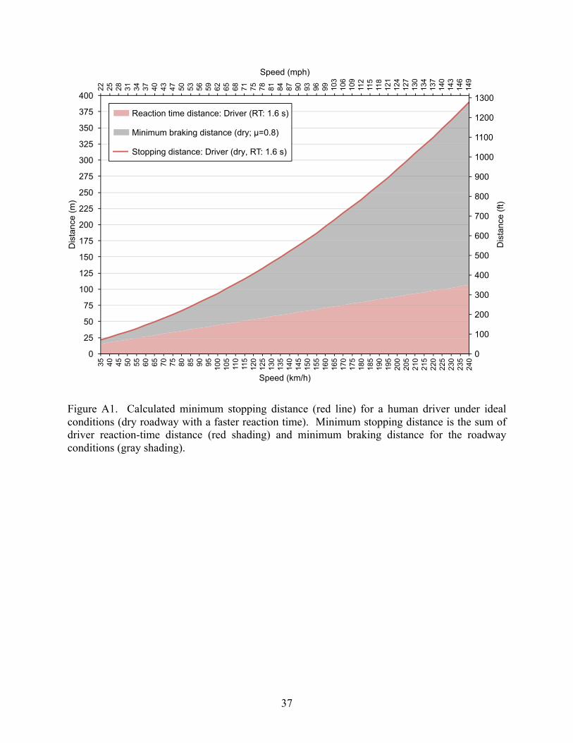
Figure A1. Calculated minimum stopping distance (red line) for a human driver under ideal conditions (dry roadway with a faster reaction time). Minimum stopping distance is the sum of driver reaction-time distance (red shading) and minimum braking distance for the roadway conditions (gray shading).

0

25

50

75

100

125

150

175

200

225

250

275

300

325

350

375

40035 40 45 50 55 60 65 70 75 80 85 90 95 100

105

110

115

120

125

130

135

140

145

150

155

160

165

170

175

180

185

190

195

200

205

210

215

220

225

230

235

240

Dis

tanc

e (m

)

Speed (km/h)

0

100

200

300

400

500

600

700

800

900

1000

1100

1200

1300

Dis

tanc

e (ft

)

22 25 28 31 34 37 40 43 47 50 53 56 59 62 65 68 71 75 78 81 84 87 90 93 96 99 103

106

109

112

115

118

121

124

127

130

134

137

140

143

146

149

Speed (mph)

Reaction time distance: Driver (RT: 1.6 s)

Minimum braking distance (dry; µ=0.8)

Stopping distance: Driver (dry, RT: 1.6 s)

38

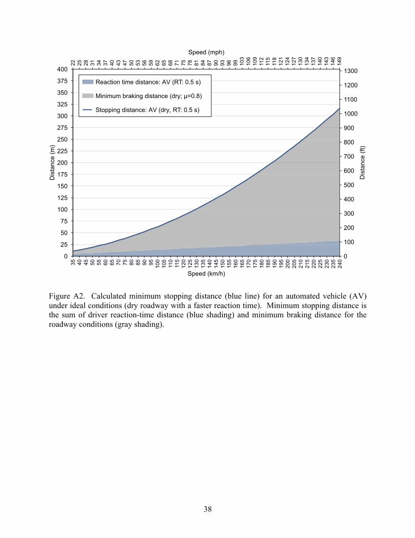
Figure A2. Calculated minimum stopping distance (blue line) for an automated vehicle (AV) under ideal conditions (dry roadway with a faster reaction time). Minimum stopping distance is the sum of driver reaction-time distance (blue shading) and minimum braking distance for the roadway conditions (gray shading).

0

25

50

75

100

125

150

175

200

225

250

275

300

325

350

375

40035 40 45 50 55 60 65 70 75 80 85 90 95 100

105

110

115

120

125

130

135

140

145

150

155

160

165

170

175

180

185

190

195

200

205

210

215

220

225

230

235

240

Dis

tanc

e (m

)

Speed (km/h)

Reaction time distance: AV (RT: 0.5 s)

Minimum braking distance (dry; µ=0.8)

Stopping distance: AV (dry, RT: 0.5 s)

0

100

200

300

400

500

600

700

800

900

1000

1100

1200

1300

Dis

tanc

e (ft

)

22 25 28 31 34 37 40 43 47 50 53 56 59 62 65 68 71 75 78 81 84 87 90 93 96 99 103

106

109

112

115

118

121

124

127

130

134

137

140

143

146

149

Speed (mph)

39

Figure A3. Calculated minimum stopping distance (red dashed line) for a human driver under degraded conditions (wet roadway with a slower reaction time). Minimum stopping distance is the sum of driver reaction-time distance (red shading) and minimum braking distance for the roadway conditions (gray shading).

0

50

100

150

200

250

300

350

400

450

500

550

600

650

700

75035 40 45 50 55 60 65 70 75 80 85 90 95 100

105

110

115

120

125

130

135

140

145

150

155

160

165

170

175

180

185

190

195

200

205

210

215

220

225

230

235

240

Dis

tanc

e (m

)

Speed (km/h)

Reaction time distance: Driver (RT: 2.5 s)

Minimum braking distance (wet; µ=0.4)

Stopping distance: Driver (wet, RT: 2.5 s)

22 25 28 31 34 37 40 43 47 50 53 56 59 62 65 68 71 75 78 81 84 87 90 93 96 99 103

106

109

112

115

118

121

124

127

130

134

137

140

143

146

149

Speed (mph)

Dis

tanc

e (ft

)

0

200

400

600

800

1000

1200

1400

1600

1800

2000

2200

2400

40

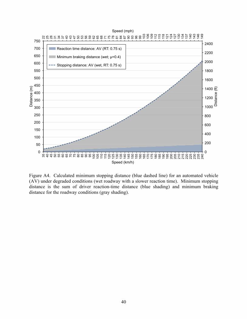
Figure A4. Calculated minimum stopping distance (blue dashed line) for an automated vehicle (AV) under degraded conditions (wet roadway with a slower reaction time). Minimum stopping distance is the sum of driver reaction-time distance (blue shading) and minimum braking distance for the roadway conditions (gray shading).

0

50

100

150

200

250

300

350

400

450

500

550

600

650

700

75035 40 45 50 55 60 65 70 75 80 85 90 95 100

105

110

115

120

125

130

135

140

145

150

155

160

165

170

175

180

185

190

195

200

205

210

215

220

225

230

235

240

Dis

tanc

e (m

)

Speed (km/h)

Reaction time distance: AV (RT: 0.75 s)

Minimum braking distance (wet; µ=0.4)

Stopping distance: AV (wet, RT: 0.75 s)

22 25 28 31 34 37 40 43 47 50 53 56 59 62 65 68 71 75 78 81 84 87 90 93 96 99 103

106

109

112

115

118

121

124

127

130

134

137

140

143

146

149

Speed (mph)

Dis

tanc

e (ft

)

0

200

400

600

800

1000

1200

1400

1600

1800

2000

2200

2400

41

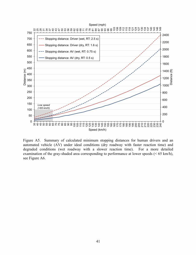
Figure A5. Summary of calculated minimum stopping distances for human drivers and an automated vehicle (AV) under ideal conditions (dry roadway with faster reaction time) and degraded conditions (wet roadway with a slower reaction time). For a more detailed examination of the gray-shaded area corresponding to performance at lower speeds (< 65 km/h), see Figure A6.

0

50

100

150

200

250

300

350

400

450

500

550

600

650

700

75035 40 45 50 55 60 65 70 75 80 85 90 95 100

105

110

115

120

125

130

135

140

145

150

155

160

165

170

175

180

185

190

195

200

205

210

215

220

225

230

235

240

Dis

tanc

e (m

)

Speed (km/h)

Stopping distance: Driver (wet, RT: 2.5 s)

Stopping distance: Driver (dry, RT: 1.6 s)

Stopping distance: AV (wet, RT: 0.75 s)

Stopping distance: AV (dry, RT: 0.5 s)

22 25 28 31 34 37 40 43 47 50 53 56 59 62 65 68 71 75 78 81 84 87 90 93 96 99 103

106

109

112

115

118

121

124

127

130

134

137

140

143

146

149

Speed (mph)

Dis

tanc

e (ft

)

0

200

400

600

800

1000

1200

1400

1600

1800

2000

2200

2400

Low speed(<65 km/h)

42

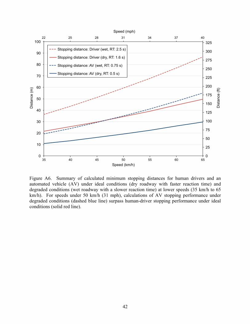
Figure A6. Summary of calculated minimum stopping distances for human drivers and an automated vehicle (AV) under ideal conditions (dry roadway with faster reaction time) and degraded conditions (wet roadway with a slower reaction time) at lower speeds (35 km/h to 65 km/h). For speeds under 50 km/h (31 mph), calculations of AV stopping performance under degraded conditions (dashed blue line) surpass human-driver stopping performance under ideal conditions (solid red line).

0

10

20

30

40

50

60

70

80

90

100

35 40 45 50 55 60 65

Dis

tanc

e (m

)

Speed (km/h)

0

25

50

75

100

125

150

175

200

225

250

275

300

325

Dis

tanc

e (ft

)

22 25 28 31 34 37 40

Speed (mph)

Stopping distance: Driver (wet, RT: 2.5 s)

Stopping distance: Driver (dry, RT: 1.6 s)

Stopping distance: AV (wet, RT: 0.75 s)

Stopping distance: AV (dry, RT: 0.5 s)