SUSTAINABLE DEVELOPMENT OF RAINFED AGRICULTURE IN INDIA John M. Kerr EPTD DISCUSSION PAPER NO. 20 with contributions by Derek Byerlee, Kumaresan Govindan, Peter Hazell, Behjat Hojjati, S. Thorat and Satya Yadav Environment and Production Technology Division International Food Policy Research Institute 1200 Seventeenth Street, N.W. Washington, D.C. 20036-3006 U.S.A. November 1996 EPTD Discussion Papers contain preliminary material and research results, and are circulated prior to a full peer review in order to stimulate discussion and critical comment. It is expected that most Discussion Papers will eventually be published in some other form, and that their content may also be revised.

Welcome message from author
This document is posted to help you gain knowledge. Please leave a comment to let me know what you think about it! Share it to your friends and learn new things together.
Transcript

SUSTAINABLE DEVELOPMENT OF RAINFED AGRICULTURE IN INDIA
John M. Kerr
EPTD DISCUSSION PAPER NO. 20
with contributions by
Derek Byerlee, Kumaresan Govindan, Peter Hazell, Behjat Hojjati,S. Thorat and Satya Yadav
Environment and Production Technology Division
International Food Policy Research Institute1200 Seventeenth Street, N.W.
Washington, D.C. 20036-3006 U.S.A.
November 1996
EPTD Discussion Papers contain preliminary material and research results, and are circulatedprior to a full peer review in order to stimulate discussion and critical comment. It is expected that mostDiscussion Papers will eventually be published in some other form, and that their content may also berevised.

ABSTRACT
India's agricultural growth has been sufficient to move the country from severe foodcrises of the 1960s to aggregate food surpluses today. Most of the increase in agriculturaloutput over the years has taken place under irrigated conditions. The opportunities forcontinued expansion of irrigated area are limited, however, so Indian planners increasinglyare looking to rainfed, or unirrigated agriculture to help meet the rising demand for foodprojected over the next several decades. Rainfed areas are highly diverse, ranging fromresource-rich areas with good agricultural potential to resource-poor areas with much morerestricted potential. Some resource-rich rainfed areas potentially are highly productive andalready have experienced widespread adoption of improved seeds. In drier, less favorableareas, on the other hand, productivity growth has lagged behind, and there is widespreadpoverty and degradation of natural resources. Even given that rainfed agriculture shouldreceive greater emphasis in public investments, a key issue is how much investment shouldbe allocated among different types of rainfed agriculture.
This paper addresses a wide variety of issues related to rainfed agriculturaldevelopment in India. It examines the historical record of agricultural productivity growthin different parts of the country under irrigated and rainfed conditions, and it reviews theevidence regarding agricultural technology development and adoption, natural resourcemanagement, poverty alleviation, risk management, and policy and institutional reform. Itpresents background information on all of these topics, offering some preliminary conclusionsand recommending areas where further research is needed. The analysis of agriculturalproductivity growth is based on district level data covering the Indo-Gangetic plains andpeninsular India from 1956 to 1990. Disaggregating the districts into a number ofagroclimatic zones to examine predominantly irrigated and rainfed zones separately providesinsights into the conditions that determined productivity growth.

i
CONTENTS
1. Introduction . . . . . . . . . . . . . . . . . . . . . . . . . . . . . . . . . . . . . . . . . . . . . . . . . . . . . . . . 1Objectives of the Paper . . . . . . . . . . . . . . . . . . . . . . . . . . . . . . . . . . . . . . . . . . . 3
2. Characteristics of Rainfed Agriculture . . . . . . . . . . . . . . . . . . . . . . . . . . . . . . . . . . . . 4Defining Rainfed Agriculture . . . . . . . . . . . . . . . . . . . . . . . . . . . . . . . . . . . . . . . 5
Rainfall Criteria . . . . . . . . . . . . . . . . . . . . . . . . . . . . . . . . . . . . . . . . . . . 5Irrigated Area Criteria . . . . . . . . . . . . . . . . . . . . . . . . . . . . . . . . . . . . . . 7
The Need for a Typology of Rainfed Agriculture . . . . . . . . . . . . . . . . . . . . . . . . 9Existing Typologies . . . . . . . . . . . . . . . . . . . . . . . . . . . . . . . . . . . . . . . . 9What a New Typology Should Look Like . . . . . . . . . . . . . . . . . . . . . . . 14
3. Performance of Rainfed Agriculture: an Overview . . . . . . . . . . . . . . . . . . . . . . . . . . 15Importance of Rainfed Agriculture in Overall Sector Performance . . . . . . . . . . 15Crop Yields in Rainfed and Irrigated Agriculture . . . . . . . . . . . . . . . . . . . . . . . 17Adoption of Modern Inputs: HYVs and Fertilizer . . . . . . . . . . . . . . . . . . . . . . . 23Patterns of Output and Yield Growth Before and Since the Green Revolution . 30
4. Growth of Output, Yields and Cropped Area: a District-level Analysis . . . . . . . . . . . 37Tabular Analysis of Growth Rates in Value of Output . . . . . . . . . . . . . . . . . . . 39
All Crops . . . . . . . . . . . . . . . . . . . . . . . . . . . . . . . . . . . . . . . . . . . . . . . 40All Cereals . . . . . . . . . . . . . . . . . . . . . . . . . . . . . . . . . . . . . . . . . . . . . . 42Individual Cereals . . . . . . . . . . . . . . . . . . . . . . . . . . . . . . . . . . . . . . . . . 44Summary Comments on the Tabular Analysis . . . . . . . . . . . . . . . . . . . . 53
Production Function Analysis of Sources of Growth in Productivity . . . . . . . . . 54
5. Technological Challenges in Rainfed Systems . . . . . . . . . . . . . . . . . . . . . . . . . . . . . 60Issues in Technology Development . . . . . . . . . . . . . . . . . . . . . . . . . . . . . . . . . 61
Seed Technology . . . . . . . . . . . . . . . . . . . . . . . . . . . . . . . . . . . . . . . . . 61Fertilizer Use . . . . . . . . . . . . . . . . . . . . . . . . . . . . . . . . . . . . . . . . . . . . 63Soil and Water Management . . . . . . . . . . . . . . . . . . . . . . . . . . . . . . . . . 64Protective Irrigation and Water Harvesting . . . . . . . . . . . . . . . . . . . . . . 65
Issues for the Future . . . . . . . . . . . . . . . . . . . . . . . . . . . . . . . . . . . . . . . . . . . . 67How Much Research? . . . . . . . . . . . . . . . . . . . . . . . . . . . . . . . . . . . . . . 67Approaches to Research . . . . . . . . . . . . . . . . . . . . . . . . . . . . . . . . . . . . 69
Watershed Management Projects . . . . . . . . . . . . . . . . . . . . . . . . . . . . . . . . . . . 77Technical Vs. Socioeconomic Orientation . . . . . . . . . . . . . . . . . . . . . . . 79The Scale of Operations . . . . . . . . . . . . . . . . . . . . . . . . . . . . . . . . . . . . 81Employment Objectives Vs. Watershed Objectives . . . . . . . . . . . . . . . . 81Watershed Evaluations Are Scarce . . . . . . . . . . . . . . . . . . . . . . . . . . . . 82
ii
6. Poverty and Rainfed Agriculture . . . . . . . . . . . . . . . . . . . . . . . . . . . . . . . . . . . . . . . 84Special Programs for Poverty Alleviation . . . . . . . . . . . . . . . . . . . . . . . . . . . . . 89Grassroots Antipoverty Initiatives That Support Rainfed Agriculture . . . . . . . . 92
7. Natural Resource Degradation and Rainfed Agriculture . . . . . . . . . . . . . . . . . . . . . . 93Soil Degradation . . . . . . . . . . . . . . . . . . . . . . . . . . . . . . . . . . . . . . . . . . . . . . . 94
Estimated Rates of Soil Erosion and its Consequences . . . . . . . . . . . . . 96Costs and Benefits of Soil Conservation Investments . . . . . . . . . . . . . 103Farmers’ Adoption of Soil Conservation Practices . . . . . . . . . . . . . . . 105Waterlogging, Salinization and Alkalinization of Irrigated Lands . . . . . 107Groundwater Degradation . . . . . . . . . . . . . . . . . . . . . . . . . . . . . . . . . 108Degradation of Uncultivated Lands . . . . . . . . . . . . . . . . . . . . . . . . . . . 111Responses to the Declining Productivity of Common Lands . . . . . . . . 113
8. Risk and Rainfed Agriculture . . . . . . . . . . . . . . . . . . . . . . . . . . . . . . . . . . . . . . . . . 118Instability of Rainfed vs. Irrigated Agriculture . . . . . . . . . . . . . . . . . . . . . . . . 118Instability Associated with Improved Agricultural Technology . . . . . . . . . . . . 119
Instability at the Farm Level . . . . . . . . . . . . . . . . . . . . . . . . . . . . . . . . 120Instability at the Aggregate Level . . . . . . . . . . . . . . . . . . . . . . . . . . . . 123
Drought Risk . . . . . . . . . . . . . . . . . . . . . . . . . . . . . . . . . . . . . . . . . . . . . . . . . 126Government Interventions to Manage Risk . . . . . . . . . . . . . . . . . . . . . . . . . . . 126
9. Infrastructure, Institutions and Policies . . . . . . . . . . . . . . . . . . . . . . . . . . . . . . . . . 133Infrastructure . . . . . . . . . . . . . . . . . . . . . . . . . . . . . . . . . . . . . . . . . . . . . . . . . 134Decentralization and Local Government . . . . . . . . . . . . . . . . . . . . . . . . . . . . . 135
Specific Institutional Issues . . . . . . . . . . . . . . . . . . . . . . . . . . . . . . . . . 139Price and Trade Policies . . . . . . . . . . . . . . . . . . . . . . . . . . . . . . . . . . . . . . . . . 142
10. Conclusions . . . . . . . . . . . . . . . . . . . . . . . . . . . . . . . . . . . . . . . . . . . . . . . . . . . . . 144District Level Data Analysis . . . . . . . . . . . . . . . . . . . . . . . . . . . . . . . . . . . . . . 144Specific Issues . . . . . . . . . . . . . . . . . . . . . . . . . . . . . . . . . . . . . . . . . . . . . . . . 147
Agricultural Research and Extension . . . . . . . . . . . . . . . . . . . . . . . . . . 147Irrigation . . . . . . . . . . . . . . . . . . . . . . . . . . . . . . . . . . . . . . . . . . . . . . 148Sustainable Use of Fragile Lands . . . . . . . . . . . . . . . . . . . . . . . . . . . . 150Infrastructure . . . . . . . . . . . . . . . . . . . . . . . . . . . . . . . . . . . . . . . . . . . 153Decentralization and Local Institutional Development . . . . . . . . . . . . . 154Other Issues . . . . . . . . . . . . . . . . . . . . . . . . . . . . . . . . . . . . . . . . . . . . 155Tradeoffs Between Investments in Different Types of Agriculture . . . . 157Steps Toward Increased Participation of Rural People . . . . . . . . . . . . 159
References . . . . . . . . . . . . . . . . . . . . . . . . . . . . . . . . . . . . . . . . . . . . . . . . . . . . . . . . . 161

John Kerr is a Research Fellow in the Environment and Production Technology*
Division of IFPRI.
SUSTAINABLE DEVELOPMENT OF RAINFED AGRICULTURE IN INDIA
John Kerr*
1. INTRODUCTION
India's agricultural growth has been sufficient to move the country from severe food
crises of the 1960s to aggregate food surpluses today. Underlying this growth were massive
public investments in irrigation, agricultural research and extension, rural infrastructure, farm
credit and rural development programs. India's agricultural sector, however, faces severe
challenges for the future. Despite sizeable national food stocks (30 million tons in 1995),
widespread poverty and hunger remain because agricultural and national economic growth
have not adequately benefitted disadvantaged regions and the poor. The demand for basic
staples, non-food grains, and exports is increasing. At the same time, resources are shrinking
and the productivity of some resources already being utilized is threatened by environmental
degradation. Growth in total factor productivity is reported to have declined slightly in major
crops. Returns to investment in agricultural research and rural infrastructure are reported to
be high, but these investments remain low.
Most of the increase in agricultural output over the years has taken place under
irrigated conditions. The opportunities for continued expansion of irrigated area are limited,
however, so Indian planners increasingly are looking to rainfed, or unirrigated agriculture to
help meet the rising demand for food projected over the next several decades. Despite the
historic bias in favor of irrigated agriculture in terms of research and infrastructural
investments, rainfed agriculture has always been an important part of the agricultural sector.
Rainfed agriculture accounts for about two-thirds of total cropped area (Government of India
1994b, nearly half of the total value of agricultural output. Nearly half of all food grains are

- 2 -
grown under rainfed conditions, and hundreds of millions of poor rural people depend on
rainfed agriculture as the primary source of their livelihoods.
Rainfed areas are highly diverse, ranging from resource-rich areas with good
agricultural potential to resource-poor areas with much more restricted potential. Some
resource-rich rainfed areas potentially are highly productive and already have experienced
widespread adoption of improved seeds. In drier, less favorable areas, on the other hand,
productivity growth has lagged behind, and there is widespread poverty and degradation of
natural resources. Even given that rainfed agriculture should receive greater emphasis in
public investments, a key issue is how much investment should be allocated among different
types of rainfed agriculture. Outmigration and income diversification into the nonagricultural
sector must provide the long term solution to economic development of many resource poor
areas, but these opportunities currently are inadequate in relation to population growth to
provide short to medium term solutions. Agricultural growth in these areas will be essential
for reducing poverty and environmental problems in the decades ahead.
There is a need to identify the opportunities for stimulating agricultural growth and
reducing poverty and environmental degradation in rainfed areas. Likewise, there is a need
to assess the opportunity costs of diverting scarce public resources from resource-rich to
resource-poor areas. The tradeoffs between investing in resource-rich and resource-poor
areas in terms of their productivity, poverty and environmental outcomes need to be
understood in order to guide public policy decisions toward productive outcomes.
Developing strategies for rainfed areas is difficult because of their diversity in terms
of agroecological characteristics, infrastructural development, and other socioeconomic
variables. On an all-India scale, for example, rainfed systems include high-rainfall agriculture
in the east and northeast as well as the drought-prone areas of the Deccan Plateau. Other
agroclimatic characteristics such as soil types also vary, as do infrastructure development,
human capital, and other socioeconomic factors. Across villages within a district, for
example, there is wide variation in access to paved roads and public transportation to market
centers. Similar diversity of agricultural systems is found even at the local level. Individual
villages in the semi-arid regions, for example, often contain numerous soil types with widely
- 3 -
differing crop production potential (Dvorak 1988). Irrigation wells are found in practically
every village, so irrigated and rainfed agriculture co-exist almost everywhere.
Diversity at both the national and local scale has implications for agricultural
development strategies. At the national scale, there is a need to distinguish among regions
according to their constraints to agricultural development. This requires creating a typology
of rainfed agriculture that would incorporate both agroecological and socioeconomic
variables in order to serve as a tool for planning agricultural research and other public
investments. Local-level diversity of rainfed agricultural systems, meanwhile, implies that
planners must recognize that changes in policy, technology or infrastructure may have varying
impacts across small areas, and that there is a limit to the extent to which external
interventions can induce finely-tuned responses. Regional or district-level planning must be
complemented by local initiatives that can be more responsive to specific needs.
OBJECTIVES OF THE PAPER
The overall goal of this paper is to review the important issues in rainfed agricultural
development and report on the progress made in India to date. This will serve as a precursor
to a detailed study to be carried out by the Indian Council of Agricultural Research, IFPRI,
ICRISAT and the World Bank. That study will result in recommendations for designing a
strategy to develop rainfed agriculture in India. In this paper, we compare the past
performance of rainfed and irrigated agriculture and of different types of rainfed agriculture,
including relatively high- and low-potential areas. We attempt to identify the factors that
determine differences in performance, and we examine the possibilities for influencing those
factors. Where information is not available, we recommend further analysis that may be
required as a prerequisite to formulating a thorough strategy for rainfed agricultural
development.
We approach the problem by reviewing the relevant literature on the subject and
conducting a statistical analysis of all-India district-level data. The database contains several
agroclimatic and socioeconomic variables that we hypothesize to influence agricultural
performance at the district level. The district-level approach, of course, does not permit

- 4 -
analysis of the implications of micro-level diversity of rainfed agricultural systems. Therefore
we focus on broader indicators with implications for area-wide development efforts.
In addition to the district level data analysis, we review the literature on rainfed
agricultural performance in terms of technology adoption and performance, yield levels and
their variability, natural resource sustainability, and poverty alleviation. We examine the role
of economic and social policies, area development programs and infrastructural investments
in promoting sustainable rainfed agricultural development. On some topics sufficient evidence
is available to draw conclusions and make policy recommendations, and on others, additional
analysis is recommended.
2. CHARACTERISTICS OF RAINFED AGRICULTURE
In this section we introduce some characteristics of rainfed agriculture that will
influence our approach to the problem of deriving recommendations to stimulate rainfed
agricultural growth.
As mentioned in the previous section, rainfed and irrigated agriculture coexist in
practically every village in India. Public investment programs, however, usually cannot be
targeted so precisely. For practical purposes, they need to be planned and implemented on
a larger scale, such as at the village, taluk, district or state level. For example, public
programs that provide credit, employ people, or build roads cannot target their efforts to
either rainfed of irrigated agriculture; they can only target areas that are relatively more
irrigated or more rainfed.
Price policies, on the other hand, can attempt to target rainfed or irrigated agriculture
within a given location by targeting crops that may be more likely to be rainfed or irrigated.
But few crops are either 100% irrigated or 100% dryland, so some spillover will always
remain. Also, every crop is grown over a large geographic area, so it is difficult to isolate the
socioeconomic and agroclimatic variables affecting their performance. And while price
policies are important, they are not the only approach through which policy makers can
influence agricultural development.
- 5 -
DEFINING RAINFED AGRICULTURE
In the present investigation we use the district as the unit of analysis. We do so for
two main reasons. First, through a district level focus our analysis may be relevant for public
investment programs that provide infrastructure or other social services to particular areas.
Second, a district focus enables us to examine the contributions of both socioeconomic and
agroclimatic variables on a nation-wide basis. The district is the smallest administrative unit
for which the required data are available. To arrive at a district-level definition of rainfed
agriculture, we consider the percentage of each district that is irrigated or rainfed, and
consider predominantly rainfed districts as "rainfed" and predominantly irrigated districts as
"irrigated." Obviously there is a certain degree of arbitrariness to any threshold we may
choose to distinguish between irrigated and rainfed districts.
Several previous studies have faced this same dilemma in categorizing rainfed areas.
Some of them have distinguished between irrigated and rainfed districts according to certain
criteria such as the amount of rainfall and the level of irrigation. Some of these studies and
their definitions of rainfed areas are listed in Table 2.1.
As mentioned above, all of these definitions suffer from the inability to distinguish
between rainfed and irrigated agriculture within districts, but we accept this as an inevitable
limitation. Another problem is that both the rainfall and irrigation thresholds are defined
somewhat arbitrarily. We discuss rainfall and irrigation thresholds in turn.
Rainfall Criteria
Among the definitions listed in table 2.1, Bapna et al, (1984) and subsequently Jodha
(1985) used broad rainfall thresholds, which is important in order not to be too exclusive. At
the same time, the 500-1500 mm range maintains a degree of homogeneity in the types of
agriculture under analysis by excluding both very dry, desert areas and very high rainfall areas.
Such areas may face unique constraints that limit comparability to agriculture under the more
moderate conditions that predominate in most of the country. Shah and Sah (1993) and
Thorat (1993) use narrow rainfall thresholds with a relatively low maximum because they
intended to focus on very dry (but not quite desert) areas. It is important to note that the
impact of the level of rainfall on crop production is conditioned by both the distribution

- 6 -
These include the pattern of rainfall distribution within the year, soil characteristics,1
altitude, temperature and slope, among other things. In India, the most important of thesefactors is probably soil type. Indian soil types range widely from moisture-retentive black claysoils (vertisols) to sandy red soils (alfisols) that hold very little moisture. Except inmountainous areas, rainfall distribution, temperature, slope and altitude all vary but notradically so.
Additional problems arise when soil types are introduced. Just as the concentration1
of irrigated area varies within districts, so does soil type. Since many districts includesignificant areas of both alfisols and vertisols (or other soil types), a single soil typespecification for a given district is bound to be somewhat inaccurate.
Table 2.1 Alternative criteria to define rainfed agriculture
Authors Criteria used
Bapnal et al Percentage of gross cropped area under irrigation (less than 25(1981) percent) and average annual rainfall (between 500 and 1500 mm)
Rangaswamy Percentage of gross cropped area under irrigation (less than 30(1981) percent) and average annual rainfall (between 375 and 1125 mm)
Jodha (1985) Percentage of gross cropped area under irrigation (less than 25percent) and average annual rainfall (between 500 mm and 1500mm)
Subbarao (1985) Percentage of gross cropped area under irrigation (less than 25percent) and average annual rainfall (less than 970 mm)
Shah and Sah Percentage of gross cropped area under irrigation (less than 25(1993) percent) and average annual rainfall (between 400 and 750 mm)
Thorat (1993) Percentage of gross cropped area under irrigation (less than 10percent) and average annual rainfall (between 375 and 750 mm)(high intensity dry farming area)
of rainfall over the course of the season and the factors that determine moisture retention in
a given location. As a result, narrow rainfall thresholds such as those used by Thorat (1993)1
are likely to combine some areas with disparate moisture regimes and separate others with
similar moisture regimes. A narrow rainfall range probably makes sense only if limited to
relatively uniform soil types. Incorporating soil types into the definition, however, introduces
yet another variable and makes the definition somewhat clumsy. For this reason, our1

- 7 -
preference is to utilize a relatively broad range of rainfall levels such as used by Bapna et al,
(1984), excluding only those that are either desert environments or extremely humid. We
choose a range of 450-1600 mm average annual rainfall as the range for predominantly rainfed
districts. The lower bound of 450 mm excludes the desert districts of western Rajasthan as
well as one district each in Punjab, Haryana and Gujarat. The 1600 mm upper bound
excludes the Himalayas, the northeastern states, Kerala, all the coastal districts of Karnataka
and Maharashtra, and one coastal district each in Tamil Nadu and Gujarat.
Where more disaggregated analysis is required to examine the performance of
relatively moist or dry rainfed areas, we can subdivide the rainfall criteria into a low rainfall
area (<750 mm per annum), a medium rainfall area (750-1125 mm), and a high rainfall area
(>1125 mm), sometimes described as the arid, semi-arid and humid areas. To repeat the
earlier caveat, these broad rainfall classes are heavily conditioned by the factors that determine
moisture retention, particularly soil type.
Irrigated Area Criteria
Classifying districts by irrigated area is difficult for several reasons. First, any
threshold percentage area irrigated must be defined somewhat arbitrarily, and second, in most
districts irrigated area has increased steadily during the period under study. As a result, we
consider some alternate approaches to categorizing districts by irrigated area.
All of the studies listed in table 2.1 use a single irrigated area threshold to distinguish
between irrigated and rainfed districts. In these studies the threshold ranges from 10 percent
to 30 percent, with most defining rainfed districts as those with less than 25 percent irrigated
area. 25 percent is the mean irrigated area for the years 1956-90, so according to this
definition, rainfed areas are those with less than average area irrigated, while irrigated areas
are those with more than average area irrigated. A number of arguments can be made about
whether the figure of 25 percent is appropriate, but ultimately any definition based on such
a threshold suffers from the problem that slight differences in irrigation levels will move some
districts from one category to the other. One approach is to use three categories of irrigation
instead of two in order to more clearly identify the characteristics of lightly and heavily
irrigated districts. This approach however, also has weaknesses, because more categories
- 8 -
means more thresholds, which means that fewer districts will remain in one category over the
entire period. As a result, when the three irrigation categories are used as described above,
nearly half of all districts shift categories at some point in the period. When only two
irrigation categories are used, on the other hand, only about one quarter of the districts shift
categories. For that reason, we also conduct the analysis with only two irrigation categories,
with districts with less than 25 percent area irrigated considered unirrigated, and districts with
25 percent or more area irrigated considered irrigated. We conduct the analysis twice; in one
case all districts are analyzed, and in the other only districts that remain in one category or the
other throughout the study period are used.
Before continuing, we briefly discuss two other criteria for defining rainfed areas that
we considered but rejected. First, districts could also be subdivided by the extent of different
types of irrigation, in particular, canals, wells, or tanks. The justification for this concerns the
quality of irrigation services delivered to each farm. Well irrigation, for example, is controlled
by the individual farmer (to the extent that the aquifer yields water), whereas under canal
irrigation farmers depend more on the amount of water taken by their upstream neighbors,
so they incur a greater risk of drought. As a result, farmers with well irrigation apply more
inputs and have much higher yields on average (Shah, 1993). The district-level data cover
gross cropped area as opposed to net cropped area, so we control for variations in the
quantity of irrigation water delivered to the farm. However, the data do not control for
variations in quality or differences in farmers’ response to the different levels of risk under
each irrigation source. When the circumstances warrant it we may examine irrigation by
source, but mainly we do not, since our main focus is on rainfed agriculture, not distinctions
in irrigated types.
A second alternative criterion for defining irrigation levels would be to distinguish
districts by the proportion of farmers who have access to some irrigation. In many areas,
water markets or shared irrigation wells enable farmers to gain access to irrigation even if they
do not own a well or are not directly serviced by a canal or a tank. As a result, the number
of farmers with access to irrigation can be much larger than the number who own wells (Shah
1993). The distinction between the proportion of area irrigated and the proportion of farmers
is important because it can affect the way in which most farmers manage their crops. If a
- 9 -
larger proportion of farmers have access to a small amount of irrigation, they may concentrate
their managerial and other inputs on irrigated plots, which they may perceive to be more
productive and less prone to risk of crop failure than dry plots. In this case, perhaps dryland
crops would be less productive (though more farmers will be better off). Farmers without
access to irrigation, on the other hand, may devote relatively more resources to rainfed crops
than those with some irrigation. Unfortunately we do not have access to district-level data
on the proportion of farmers with access to irrigation, and we do not know if the proportion
of farmers with access to irrigation and the proportion of area irrigated vary independently
of each other across districts. Therefore we cannot consider using this definition; we raise
it only to draw attention to some of the issues to consider in developing a definition of a
rainfed district.
THE NEED FOR A TYPOLOGY OF RAINFED AGRICULTURE
The definition of rainfed agriculture presented in the previous section will assist us in
comparing the performance of predominantly rainfed and irrigated districts. We also wish to
compare the performance within rainfed agricultural districts and relate differences to a range
of constraints to agricultural development. This in turn will be useful for prioritizing and
organizing agricultural research, public investment, and policy and institutional reform. To
characterize districts according to the various agroclimatic and socioeconomic variables that
constrain agricultural development, we will need to construct a typology based on those
variables. In this section we discuss in a bit more detail the typologies of Indian rainfed
agriculture that already exist, the reasons why a new typology needs to be constructed, and
the ways in which such a typology would be used.
Existing Typologies
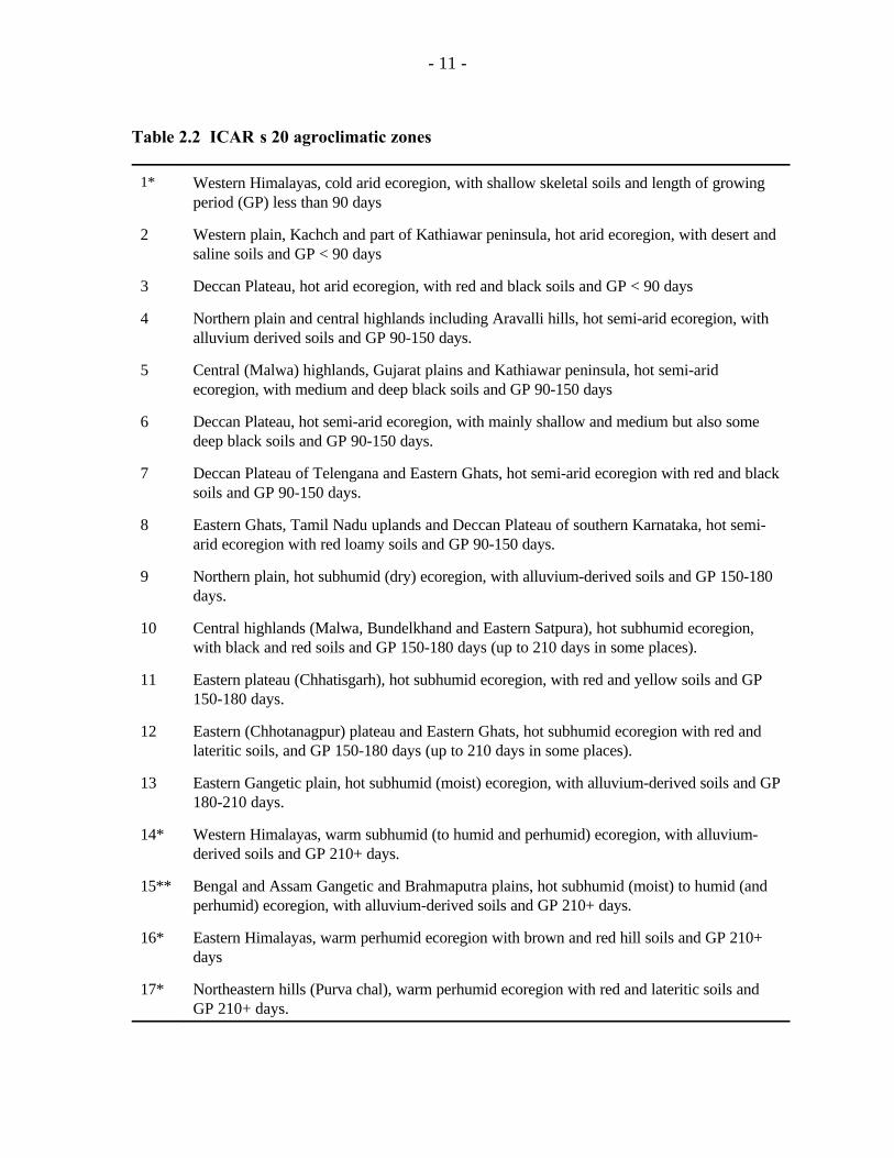
Current typologies of Indian agriculture are based on agroecological zones. Recently,
ICAR delineated 20 agroclimatic regions based on soils and climate (NBSS&LUP, 1992).
13 of these zones cover the area of this study; of the rest, 5 are in the Northeast, the
Himalayas, and the Andaman, Nicobar and Lakshadweep Islands; one zone covers the high
rainfall areas of the Western Ghats and the Arabian Sea coast; and one zone covers the desert

- 10 -
in the western parts of Rajasthan and Gujarat. Figure 2.1 displays the 20 zones, and table 2.2
presents some distinguishing features of each.
ICAR’s agroecological zoning system is based on variations in rainfall, soil type and
temperature. Irrigation status, however, is conspicuously absent. This is a severe limitation
due to the primary importance of irrigation in determining cropping patterns and productivity
in most of the country. In this analysis we overcome that shortcoming by dividing zones into
primarily rainfed and primarily irrigated districts. We discuss this division further below.
The 20-zone system is sufficiently disaggregated to enable it to keep problems of
within-zone variation to a manageable level, and the number of zones remains small enough
to be manageable for most uses. Also, the zones can be easily reaggregated for particular
purposes. Recently ICAR subdivided the 20-zone typology into a total of about 50 subzones;
such a disaggregated typology may be useful for certain agricultural research purposes, but
for policy analysis it is too large to be functional.
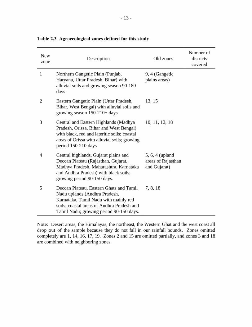
In our analysis, using rainfed and irrigated districts in the 13 zones covered in our data
would yield a total of 26 categories, which becomes unmanageable. For the purposes of our
district-level analysis, we modify the 20-zone system so that it is sufficiently aggregated for
our purposes. We create a new 5-zone system in which each zone is a combination of two
or more of the zones of the 20-zone system.
The new zones, shown in table 2.3, require some explanation. First, the 20-zone
system does not follow district boundaries, but in our analysis districts must remain intact.
As a result, in many cases we classify a district as lying in one zone even though part of it may
actually lie in another. Districts in ICAR’s Zone 18 along the Bay of Bengal coast, for
example, also lie in adjoining agroclimatic zones 7,8 and 12. As a result, zone 18 drops out
of the sample. Second, by combining the zones it is inevitable that some new, aggregated
zones will contain substantial within-zone diversity. We find that for the case of ICAR zone
4, it makes sense to place the portion of zone 4 that lies in the Gangetic plain in one new
zone, and the part that lies in upland areas of Rajasthan and Gujarat in another.
- 11 -
Table 2.2 ICAR’s 20 agroclimatic zones
1* Western Himalayas, cold arid ecoregion, with shallow skeletal soils and length of growingperiod (GP) less than 90 days
2 Western plain, Kachch and part of Kathiawar peninsula, hot arid ecoregion, with desert andsaline soils and GP < 90 days
3 Deccan Plateau, hot arid ecoregion, with red and black soils and GP < 90 days
4 Northern plain and central highlands including Aravalli hills, hot semi-arid ecoregion, withalluvium derived soils and GP 90-150 days.
5 Central (Malwa) highlands, Gujarat plains and Kathiawar peninsula, hot semi-aridecoregion, with medium and deep black soils and GP 90-150 days
6 Deccan Plateau, hot semi-arid ecoregion, with mainly shallow and medium but also somedeep black soils and GP 90-150 days.
7 Deccan Plateau of Telengana and Eastern Ghats, hot semi-arid ecoregion with red and blacksoils and GP 90-150 days.
8 Eastern Ghats, Tamil Nadu uplands and Deccan Plateau of southern Karnataka, hot semi-arid ecoregion with red loamy soils and GP 90-150 days.
9 Northern plain, hot subhumid (dry) ecoregion, with alluvium-derived soils and GP 150-180days.
10 Central highlands (Malwa, Bundelkhand and Eastern Satpura), hot subhumid ecoregion,with black and red soils and GP 150-180 days (up to 210 days in some places).
11 Eastern plateau (Chhatisgarh), hot subhumid ecoregion, with red and yellow soils and GP150-180 days.
12 Eastern (Chhotanagpur) plateau and Eastern Ghats, hot subhumid ecoregion with red andlateritic soils, and GP 150-180 days (up to 210 days in some places).
13 Eastern Gangetic plain, hot subhumid (moist) ecoregion, with alluvium-derived soils and GP180-210 days.
14* Western Himalayas, warm subhumid (to humid and perhumid) ecoregion, with alluvium-derived soils and GP 210+ days.
15** Bengal and Assam Gangetic and Brahmaputra plains, hot subhumid (moist) to humid (andperhumid) ecoregion, with alluvium-derived soils and GP 210+ days.
16* Eastern Himalayas, warm perhumid ecoregion with brown and red hill soils and GP 210+days
17* Northeastern hills (Purva chal), warm perhumid ecoregion with red and lateritic soils andGP 210+ days.

- 12 -
Table 2.2 (continued)
18 Eastern coastal plain, hot subhumid to semi-arid ecoregion, with coastal alluvium-derivedsoils and GP 90-210+ days.
19* Western ghats and coastal plain, hot humid-perhumid ecoregion with red, lateritic andalluvium-derived soils, and GP 210+ days.
20* Islands of Andaman-Nicobar and Lakshadweep hot humid to perhumid island ecoregion,with red loamy and sandy soils, and GP 210+ days.
* Indicates zones not included in the district level data.** District level data contains Zone 13 districts in West Bengal but not Assam.
Source: NBSS&LUP, 1992
- 13 -
Table 2.3 Agroecological zones defined for this study
Newzone
Description Old zones districtsNumber of
covered
1 Northern Gangetic Plain (Punjab, 9, 4 (GangeticHaryana, Uttar Pradesh, Bihar) with plains areas)alluvial soils and growing season 90-180days
2 Eastern Gangetic Plain (Uttar Pradesh, 13, 15Bihar, West Bengal) with alluvial soils andgrowing season 150-210+ days
3 Central and Eastern Highlands (Madhya 10, 11, 12, 18Pradesh, Orissa, Bihar and West Bengal)with black, red and lateritic soils; coastalareas of Orissa with alluvial soils; growingperiod 150-210 days
4 Central highlands, Gujarat plains and 5, 6, 4 (uplandDeccan Plateau (Rajasthan, Gujarat, areas of RajasthanMadhya Pradesh, Maharashtra, Karnataka and Gujarat)and Andhra Pradesh) with black soils;growing period 90-150 days.
5 Deccan Plateau, Eastern Ghats and Tamil 7, 8, 18Nadu uplands (Andhra Pradesh,Karnataka, Tamil Nadu with mainly redsoils; coastal areas of Andhra Pradesh andTamil Nadu; growing period 90-150 days.
Note: Desert areas, the Himalayas, the northeast, the Western Ghat and the west coast alldrop out of the sample because they do not fall in our rainfall bounds. Zones omittedcompletely are 1, 14, 16, 17, 19. Zones 2 and 15 are omitted partially, and zones 3 and 18are combined with neighboring zones.

- 14 -
What a New Typology Should Look Like
The existing agroclimatic typologies may be adequate for a narrow set of objectives,
such as locating where certain crops are likely to be produced and which regions may be
prone to certain natural resource management problems. Beyond such highly specific
applications, however, the agroclimatic typologies are of limited use because they are so
narrowly defined.
In order to be useful for designing a strategy to develop rainfed agriculture, a typology
must be constructed on the basis of the whole range of factors that affect agricultural
development. These extend far beyond simple agroclimatic conditions or even irrigation
status. If a district has favorable growing conditions but lacks the infrastructure needed to
support productive farming, for example, it should not be surprising to find poor performance
in that district despite the favorable agroclimatic conditions. Later in the paper we will
examine the determinants of agricultural performance and demonstrate that other factors in
addition to agroclimatic conditions help explain the variation in performance.
In addition to agroclimatic conditions and irrigation status, numerous additional
variables can be hypothesized to influence agricultural development. Physical infrastructure
such as roads and electrification, for example, and social infrastructure such as banks, markets
and agricultural research and extension services, can be expected to play an important role
in stimulating the agricultural sector. Demographic indicators such as population density and
literacy levels also may be related to agricultural performance, as may economic policies that
directly or indirectly affect input or output prices. Institutional considerations also may affect
performance; they include laws governing trade, property rights, prices of inputs and outputs,
etc., and the quality of services provided by government agencies.
Just as there are many determinants of performance of the agricultural sector, there
also are many criteria for evaluating performance. Productivity growth is one that is
commonly applied, but others include the levels of poverty and food security, the variability
of production and income, and the degree of degradation of natural resources.
The ideal typology of Indian agriculture would characterize regions or areas according
to all the factors that determine performance over a broad range of criteria. In this way it
could serve as a valuable planning tool for public investment in agricultural research,

- 15 -
infrastructural development, poverty alleviation programs, policy and institutional reform, etc.
While such a "super typology" might be unattainable, it presents an objective to work toward.
In preparing this paper we lack the resources to develop an acceptable typology, but it
remains a high priority for future research intended to support Indian rainfed agricultural
development.
Later in the paper we analyze the determinants of rainfed agricultural development
using multiple regression analysis. We will identify many of the agroclimatic and
socioeconomic factors that contribute to performance of Indian rainfed agriculture according
to a variety of criteria. We will stop short of creating a typology, but we will gain preliminary
indications of the kinds of information that need to go into such a typology.
3. PERFORMANCE OF RAINFED AGRICULTURE: AN OVERVIEW
In this section we begin with some summary statistics of rainfed and irrigated
agriculture, and then scrutinize differences in their growth rates for different crops over space
and time. Section 3 reviews the relevant literature, and section 4 presents an analysis based
on district-level data.
IMPORTANCE OF RAINFED AGRICULTURE IN OVERALL SECTORPERFORMANCE
Rainfed agriculture is clearly critical to agricultural performance in India.
Nonetheless, it is difficult to precisely quantify the overall importance of the sector. The
widely quoted statistic is that 70% of cultivated area is rainfed, implying that rainfed
agriculture is more important than irrigated agriculture. However, this statistic grossly
overstates the importance of rainfed agriculture in the economy for several reasons:
1. Since cropping intensity is lower in rainfed areas, the proportion of gross cropped
area in rainfed areas was 66% in 1992.
2. Rainfed yields are on average less than half of irrigated yields (for food grains), so that
the proportion of food grains produced in rainfed areas was 43% in the late 1980s
(Planning Commission 1986). For non-food grains, the yield difference is even
- 16 -
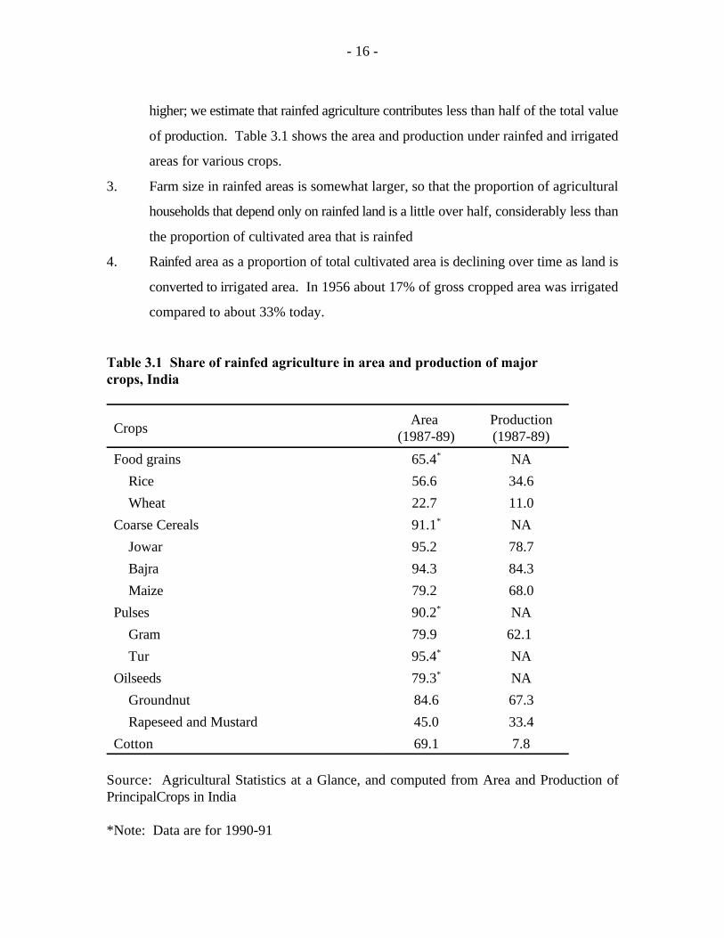
higher; we estimate that rainfed agriculture contributes less than half of the total value
of production. Table 3.1 shows the area and production under rainfed and irrigated
areas for various crops.
3. Farm size in rainfed areas is somewhat larger, so that the proportion of agricultural
households that depend only on rainfed land is a little over half, considerably less than
the proportion of cultivated area that is rainfed
4. Rainfed area as a proportion of total cultivated area is declining over time as land is
converted to irrigated area. In 1956 about 17% of gross cropped area was irrigated
compared to about 33% today.
Table 3.1 Share of rainfed agriculture in area and production of majorcrops, India
CropsArea Production
(1987-89) (1987-89)
Food grains 65.4 NA*
Rice 56.6 34.6
Wheat 22.7 11.0
Coarse Cereals 91.1 NA*
Jowar 95.2 78.7
Bajra 94.3 84.3
Maize 79.2 68.0
Pulses 90.2 NA*
Gram 79.9 62.1
Tur 95.4 NA*
Oilseeds 79.3 NA*
Groundnut 84.6 67.3
Rapeseed and Mustard 45.0 33.4
Cotton 69.1 7.8
Source: Agricultural Statistics at a Glance, and computed from Area and Production ofPrincipalCrops in India
*Note: Data are for 1990-91

- 17 -
Against this background, there may be counterbalancing factors that would increase
the weight to rainfed areas in development strategies. First, if sources of yield growth in
irrigated areas are being exhausted and there are low returns to additional intensification in
irrigated areas, then the potential role of rainfed areas in the future will increase. In a later
section, we briefly examine the evidence on yield potential in rainfed areas.
Second, to the extent that other development objectives, especially poverty alleviation
and conservation of the natural resource base, are important, rainfed areas merit increased
attention relative to their weight in agricultural income generation. In another section of this
report, we have established that the poorest groups of the population depend on rainfed
agriculture and that given the emphasis of the GOI and the Bank on poverty alleviation,
rainfed agriculture deserves greater attention.
CROP YIELDS IN RAINFED AND IRRIGATED AGRICULTURE
A conventional wisdom that is widely held in the development community both inside
and outside of India is that rainfed agriculture has been technologically stagnant. In part, this
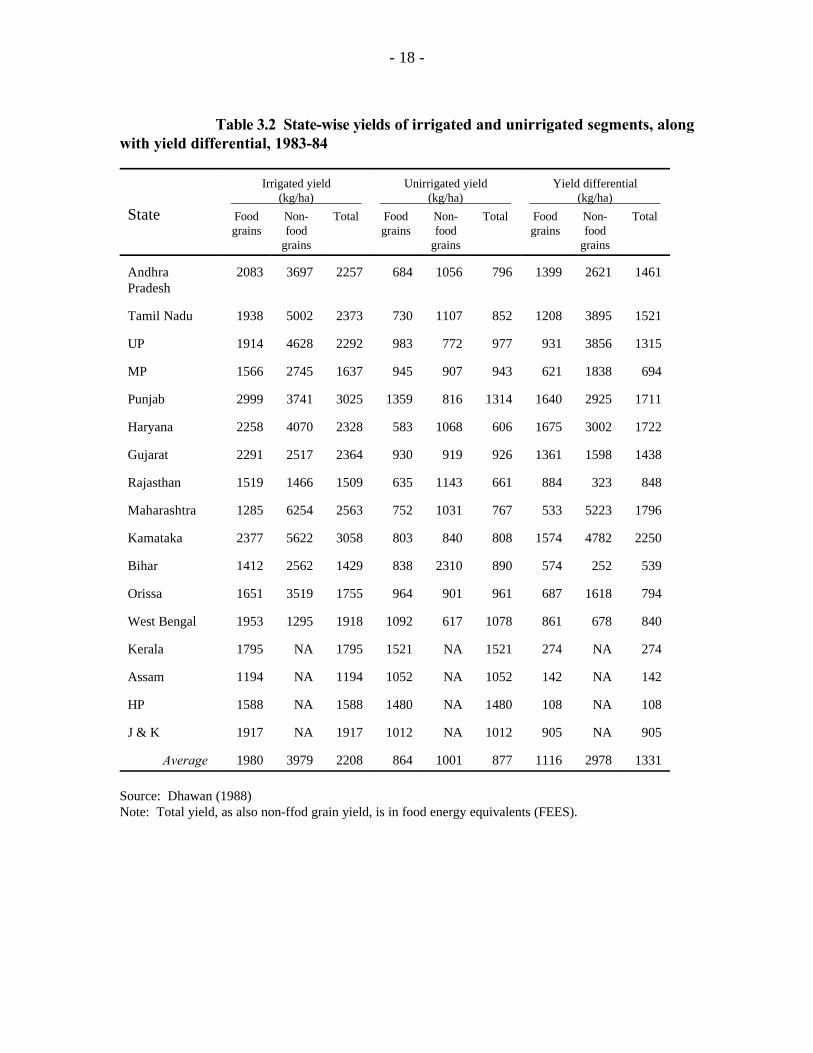
arises from comparisons of yields and input use between rainfed and irrigated areas. Dhawan,
for example, has commented in several publications that the high yields in irrigated agriculture
indicate the need for greater investment in the irrigated sector (Dhawan, 1988a). Table 3.2,
for example, shows Dhawan’s comparison of irrigated and rainfed crop yields for the year
1983-84. In most of the country, irrigated yields surpass rainfed yields by about 1-2 tons/ha,
though in the wetter states of the Himalayas, the northeast, and Kerala the difference is
smaller. These yield differences, while significant, are of only limited use because they do not
control for differences in the composition of crops grown.
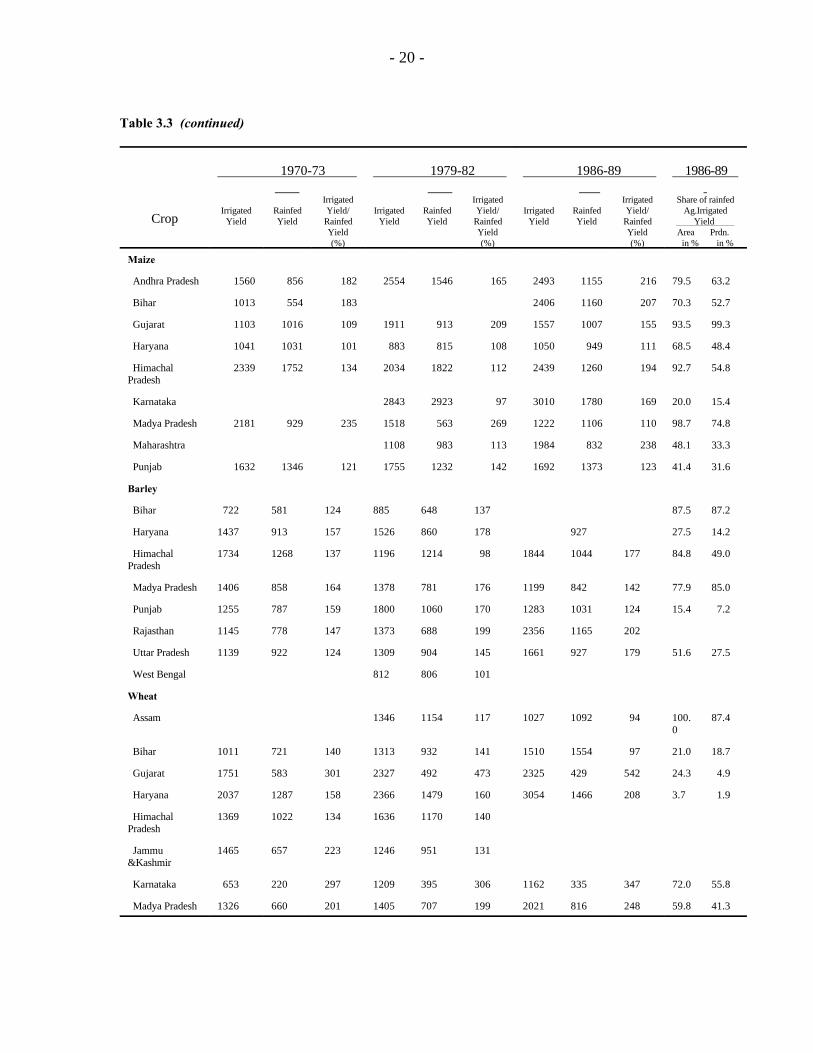
Table 3.3 presents average crop yields for irrigated and rainfed conditions in different
states for the periods 1970-73, 1979-82, and 1986-89. It shows that irrigated yields are
generally much higher than rainfed yields, as expected. In many cases yield gaps are widening
over time in favor of irrigated areas. The difference is consistently high for cotton and quite
high also for sorghum (though this excludes data for Maharashtra, which has the
- 18 -
Table 3.2 State-wise yields of irrigated and unirrigated segments, alongwith yield differential, 1983-84
State
Irrigated yield Unirrigated yield Yield differential (kg/ha) (kg/ha) (kg/ha)
Food Non- Total Food Non- Total Food Non- Totalgrains food grains food grains food
grains grains grains
Andhra 2083 3697 2257 684 1056 796 1399 2621 1461Pradesh
Tamil Nadu 1938 5002 2373 730 1107 852 1208 3895 1521
UP 1914 4628 2292 983 772 977 931 3856 1315
MP 1566 2745 1637 945 907 943 621 1838 694
Punjab 2999 3741 3025 1359 816 1314 1640 2925 1711
Haryana 2258 4070 2328 583 1068 606 1675 3002 1722
Gujarat 2291 2517 2364 930 919 926 1361 1598 1438
Rajasthan 1519 1466 1509 635 1143 661 884 323 848
Maharashtra 1285 6254 2563 752 1031 767 533 5223 1796
Kamataka 2377 5622 3058 803 840 808 1574 4782 2250
Bihar 1412 2562 1429 838 2310 890 574 252 539
Orissa 1651 3519 1755 964 901 961 687 1618 794
West Bengal 1953 1295 1918 1092 617 1078 861 678 840
Kerala 1795 NA 1795 1521 NA 1521 274 NA 274
Assam 1194 NA 1194 1052 NA 1052 142 NA 142
HP 1588 NA 1588 1480 NA 1480 108 NA 108
J & K 1917 NA 1917 1012 NA 1012 905 NA 905
Average 1980 3979 2208 864 1001 877 1116 2978 1331
Source: Dhawan (1988)Note: Total yield, as also non-ffod grain yield, is in food energy equivalents (FEES).

- 19 -
Table 3.3 State-wise irrigated and rainfed yields of major crops and the share of rainfed agriculturein area and production
1970-73 1979-82 1986-89 1986-89
Crop Irrigated Rainfed Yield/ Irrigated Rainfed Yield/ Irrigated Rainfed Yield/ Ag.IrrigatedYield Yield Rainfed Yield Yield Rainfed Yield Yield Rainfed Yield
Irrigated Irrigated Irrigated Share of rainfed
Yield Yield Yield Area Prdn. (%) (%) (%) in % in %
Rice
Andhra Pradesh 1512 691 219 1986 833 238 2134 746 286 5.8 2.9
Assam 1353 805 1412 778 181 66.2 54.7
Bihar 880 533 165 1278 621 206 1258 791 159 64.2 56.0
Gujarat 1762 1144 154 1772 947 187 2232 983 227 57.0 35.1
Himachal 1337 945 141 1454 956 152 1263 1229 103 45.8 45.9Pradesh
Karnataka 1771 1243 142 1852 1544 120 2350 1336 176 39.0 23.6
Kerala 1577 1242 127 1430 1290 111 1775 1433 124 55.0 27.1
Madya Pradesh 1095 741 148 1083 633 171 1454 793 183 79.0 71.4
Maharashtra 909 767 119 1535 1443 106 1305 1207 108 74.2 68.0
Orissa 1007 910 111 1153 653 176 1139 688 166 66.8 43.0
Punjab 1979 1296 153 2460 1018 242 3278 1155 284 1.2 0.4
Rajasthan 1511 553 273 2204 1129 195 58.5 57.7
Tamil Nadu 1990 1012 197 2064 862 239 3256 969 336 8.5 1.7
Uttar Pradesh 1247 758 164 1581 1163 136 66.8 54.9
West Bengal 1683 1012 166 1513 784 193 1663 1013 164 75.4 46.9
Jowar
Andhra Pradesh 523 292 179 1316 573 230 1511 589 257 98.4 92.9
Gujarat 829 221 375 1302 467 279 680 278 245 97.2 78.6
Haryana 265 260 102 316 214 147 318 109 292 67.1 27.7
Karnataka 1329 720 185 1132 876 129 2677 1100 243 93.0 60.9
Madya Pradesh 187 1042 703 148 758 99.9 98.6
Maharashtra 419 1050 1105 94.2 69.7
Tamil Nadu 1313 584 225 1638 748 219 2425 908 267 92.7 93.9
Bajra
Andhra Pradesh 1050 367 286 1508 586 257 1031 508 203 89.0 77.8
Gujarat 1100 717 153 1302 878 148 1026 572 179 90.9 79.7
Haryana 843 594 142 845 557 152 917 531 173 84.6 96.7
Karnataka 949 174 545 689 361 191 1064 482 221 91.5 95.1
- 20 -
Table 3.3 (continued)
1970-73 1979-82 1986-89 1986-89
CropIrrigated Rainfed Yield/ Irrigated Rainfed Yield/ Irrigated Rainfed Yield/ Ag.Irrigated
Yield Yield Rainfed Yield Yield Rainfed Yield Yield Rainfed Yield
Irrigated Irrigated Irrigated Share of rainfed
Yield Yield Yield Area Prdn. (%) (%) (%) in % in %
Maize
Andhra Pradesh 1560 856 182 2554 1546 165 2493 1155 216 79.5 63.2
Bihar 1013 554 183 2406 1160 207 70.3 52.7
Gujarat 1103 1016 109 1911 913 209 1557 1007 155 93.5 99.3
Haryana 1041 1031 101 883 815 108 1050 949 111 68.5 48.4
Himachal 2339 1752 134 2034 1822 112 2439 1260 194 92.7 54.8Pradesh
Karnataka 2843 2923 97 3010 1780 169 20.0 15.4
Madya Pradesh 2181 929 235 1518 563 269 1222 1106 110 98.7 74.8
Maharashtra 1108 983 113 1984 832 238 48.1 33.3
Punjab 1632 1346 121 1755 1232 142 1692 1373 123 41.4 31.6
Barley
Bihar 722 581 124 885 648 137 87.5 87.2
Haryana 1437 913 157 1526 860 178 927 27.5 14.2
Himachal 1734 1268 137 1196 1214 98 1844 1044 177 84.8 49.0Pradesh
Madya Pradesh 1406 858 164 1378 781 176 1199 842 142 77.9 85.0
Punjab 1255 787 159 1800 1060 170 1283 1031 124 15.4 7.2
Rajasthan 1145 778 147 1373 688 199 2356 1165 202
Uttar Pradesh 1139 922 124 1309 904 145 1661 927 179 51.6 27.5
West Bengal 812 806 101
Wheat
Assam 1346 1154 117 1027 1092 94 100. 87.40
Bihar 1011 721 140 1313 932 141 1510 1554 97 21.0 18.7
Gujarat 1751 583 301 2327 492 473 2325 429 542 24.3 4.9
Haryana 2037 1287 158 2366 1479 160 3054 1466 208 3.7 1.9
Himachal 1369 1022 134 1636 1170 140Pradesh
Jammu 1465 657 223 1246 951 131&Kashmir
Karnataka 653 220 297 1209 395 306 1162 335 347 72.0 55.8
Madya Pradesh 1326 660 201 1405 707 199 2021 816 248 59.8 41.3

- 21 -
Table 3.3 (continued)
1970-73 1979-82 1986-89 1986-89
CropIrrigated Rainfed Yield/ Irrigated Rainfed Yield/ Irrigated Rainfed Yield/ Ag.Irrigated
Yield Yield Rainfed Yield Yield Rainfed Yield Yield Rainfed Yield
Irrigated Irrigated Irrigated Share of rainfed
Yield Yield Yield Area Prdn. (%) (%) (%) in % in %
Maharashtra 1107 524 211 1233 599 206 44.1 20.5
Punjab 2393 1112 215 2887 1489 194 3310 1752 189 5.1 3.3
Rajasthan 1441 749 192 1622 808 201 2159 1257 172 9.8 6.4
Uttar Pradesh 1422 910 156 1667 948 176 2006 1257 160 14.1 9.1
West Bengal 1429 971 147
Gram
Gujarat 1127 666 169 1027 635 162 877 489 179 73.6 65.2
Haryana 845 553 153 552 450 123 733 527 139 66.1 41.3
Karnataka 348 123 283 588 438 134 512 429 119 91.7 11.2
Madya Pradesh 812 623 130 931 536 174 825 640 129 82.9 80.5
Maharashtra 530 332 160 567 383 148 77.0 67.1
Punjab 870 722 120 622 477 130 623 477 131 86.8 54.9
Rajasthan 887 564 157 814 522 156 806 716 113 74.9 75.2
Uttar Pradesh 823 750 110 760 637 119 1041 716 145 82.6 75.9
Groundnut
Andhra Pradesh 1016 719 141 1160 705 164 948 808 117 81.5 69.8
Gujarat 1051 927 113 929 791 117 1593 680 234 91.6 68.2
Karnataka 1616 1345 120 964 629 153 970 647 150 79.7 65.3
Madya Pradesh 630 642 98 1189 923 129 94.3 91.2
Maharashtra 1400 682 205 967 752 129 97.3 78.3
Punjab 980 1022 96 1151 933 123 920 412 223 47.5 22.1
Rajasthan 1388 592 235 951 510 187 1195 761 157 67.8 64.9
Tamil Nadu 1539 903 170 1649 820 201 1838 943 195 73.8 61.4
Cotton
Andhra Pradesh 308 70 440 387 184 211 746 311 240 77.8 16.3
Gujarat 306 165 185 358 133 269 387 89 435 67.1 3.9
Karnataka 134 23 583 310 83 374 419 122 343 81.6 4.8
Madya Pradesh 140 73 192 293 110 266 11.0 14.1
Maharashtra 246 46 535 210 86 245 293 76 386 96.0 9.0
Rajasthan 217 106 205 213 63 338 391 206 190 5.8 0.5
Tamil Nadu 312 71 439 375 77 485 445 167 266 59.7 5.7
Source: Area and Production of Principal Crops in India, Various issues

- 22 -
highest rainfed sorghum yield of any state). The difference is consistently smaller for gram.
For other crops, the gap varies substantially by state; more information would be needed on
the agroclimatic conditions under which these crops are being grown in order to say more
about the reasons for differences in relative yields.
The yield comparisons between irrigated and rainfed agriculture are not surprising,
but they should not be the sole basis for comparison between rainfed and irrigated agriculture.
Rainfed yields and input use will always lag behind those in irrigated areas, so other
performance measures must be used. In fact, there are many indicators of remarkable success
in technology adoption and yield growth in rainfed agriculture in India. Examples include the
following:
C The rapid shifts of cropping patterns and adoption of new crops in rainfed areas
(Kelley and Parthasarathy Rao 1994). The recent widespread adoption of new oilseed
crops, especially soyabeans and sunflowers, in central and southern India is testimony
to the potential for rapid change in rainfed areas, given appropriate technology, input
and marketing support, and policy incentives (Singh et al). The rapid and broadly
based growth of the cotton sector is further testimony to the potential for these types
of changes.
! The relatively high growth performance in yields of some crops that are grown largely
under rainfed conditions. This is most apparent for cash crops, especially cotton and
oilseeds but is also evident for some food grains in some states (e.g. sorghum in
Maharashtra, pearl millet in Gujarat, finger millet (ragi) in Karnataka, and maize and
pigeon pea in some districts).
! The overall growth of total factor productivity of 1% annually in agroclimatic zones
that depend largely on rainfed agriculture (Evenson, Pray and Rosegrant, 1995).
Although this growth rate lags behind the 1.5% rate observed in the Green Revolution
areas of northwest India, the difference is surprisingly small.
Nonetheless, the overall growth of rainfed agriculture has been slow. This is evident
in overall statistics for coarse grains and especially pulses, and rising real prices for some

- 23 -
crops such as pulses that are largely grown in rainfed areas (Kelley and Parthasarathy Rao,
1994). In a few states where there are fairly complete and reliable data on irrigated and
rainfed yields, the growth rate of rainfed yields has generally lagged. For example, for the
period 1960-85, rainfed wheat yields increased at a rate of 1.4% annually, only half of that
observed in irrigated areas (Byerlee, 1992). Yields of rainfed rice lagged irrigated yields until
1980 but showed remarkable growth thereafter, especially in West Bengal (table 3.3 and table
3.4). Table 3.4 shows changes in growth rates over time under irrigated and rainfed
conditions between 1970 and 1989. Patterns vary by crop and region, and clear patterns are
difficult to discern.
ADOPTION OF MODERN INPUTS: HYVs AND FERTILIZER
The significant success stories for rainfed areas reflect widespread adoption of modern
inputs, especially improved seed and fertilizers. One of the best kept secrets of Indian
agriculture (at least from the point of view of an outside observer of Indian agriculture) has
been the remarkable spread of HYVs in rainfed areas beginning in the mid-1970s and
accelerating in the past decade. In 1976, 84% of the HYV area was under irrigation
(calculated from table 27 of Desai, 1982). By the early 1990s over 40% of the area of HYVs
was sown in rainfed areas. From about 1976, the cereal area sown to HYVs has exceeded
the irrigated area of cereals, and this gap has widened over time. We estimate that in the
1980s, an additional 22 million ha of cereal area was sown to HYVs. Of this amount, 16
million ha or nearly three quarters of the total area expansion occurred in rainfed areas. This
represents the most spectacular example of widespread adoption of HYVs by small-scale
farmers under rainfed conditions in the world. The following statistics and assumptions,
drawn mainly from table 3.5 (NCAER 1990), elaborate on these calculations.
! The largest expansion in area of HYVs has been for rice in eastern India. HYVs are
now sown on 50% of the rice area in Eastern India compared to only 20% of the rice
area that is irrigated.
! The next largest expansion has been in coarse grains, nearly all under rainfed
conditions, especially sorghum in Maharashtra, pearl millet in Gujarat and ragi

- 24 -
Table 3.4 Growth rates of state-wise irrigated and rainfed crop yields
Growth Rates (%) 1970-73 - 1979-82 1979-82 - 1986-89 1970-73 - 1986-89
Crop Irrigated Rainfed Irrigated Rainfed Irrigated RainfedYield Yield Yield Yield Yield Yield
Rice
Andhra Pradesh 3.08 2.11 1.03 -1.56 2.18 0.48
Assam 0.62 -0.48
Bihar 4.23 1.71 -0.23 3.53 2.26 2.50
Gujarat 0.07 -2.08 3.35 0.53 1.49 -0.95
Himachal Pradesh 0.94 0.12 -1.99 3.65 -0.35 1.65
Karnataka 0.50 2.43 3.46 -2.04 1.78 0.45
Kerala -1.08 0.42 3.14 1.52 0.74 0.90
Madya Pradesh -0.12 -1.74 4.30 3.28 1.79 0.43
Maharashtra 5.99 7.29 -2.29 -2.52 2.29 2.88
Orissa 1.51 -3.62 -0.17 0.75 0.77 -1.73
Punjab 2.45 -2.64 4.18 1.82 3.20 -0.72
Rajasthan 5.54 10.73
Tamil Nadu 0.40 -1.77 6.73 1.69 3.12 -0.27
Uttar Pradesh 3.44 6.30
West Bengal -1.18 -2.80 1.36 3.74 -0.07 0.01
Jowar
Andra Pradesh 10.80 7.77 1.99 0.40 6.86 4.48
Gujarat 5.14 8.67 -6.96 5.51 -1.23 7.28
Haryana 1.96 -2.11 0.11 -9.21 1.15 -5.28
Karnataka -1.77 2.20 13.08 3.31 4.47 2.69
Madya Pradesh 15.86 1.08 9.14
Maharashtra 10.77 0.73 6.26
Tamil Nadu 2.49 2.78 5.77 2.81 3.91 2.80
Bajra
Andhra Pradesh 4.10 5.33 -5.29 -2.01 -0.11 2.05
Gujarat 1.88 2.28 -3.34 -5.94 -0.44 -1.40

- 25 -
Table 3.4 (continued)
Growth Rates (%) 1970-73 - 1979-82 1979-82 - 1986-89 1970-73 - 1986-89
Crop Irrigated Rainfed Irrigated Rainfed Irrigated RainfedYield Yield Yield Yield Yield Yield
Haryana 0.03 -0.71 1.18 -0.69 0.53 -0.70
Karnataka -3.49 8.44 6.40 4.23 0.72 6.58
Madya Pradesh 13.68 -4.64 7.82 0.62
Maharashtra 8.07 10.57 0.06 -2.04 4.49 4.87
Punjab 0.06 -0.70 2.00 -0.04 0.90 -0.41
Rajasthan -0.05 13.60
Tamil Nadu 3.55 3.65 3.37 5.60 3.47 4.50
Maize
Andhra Pradesh 5.63 6.79 -0.34 -4.08 2.97 1.89
Bihar 5.55 4.73
Gujarat 6.30 -1.18 -2.89 1.41 2.18 -0.06
Haryana -1.82 -2.57 2.51 2.19 0.05 -0.51
Himachal Pradesh -1.54 0.44 2.63 -5.13 0.26 -2.04
Karnataka 0.82 -6.84
Madya Pradesh -3.95 -5.41 -3.05 10.12 -3.56 1.10
Maharashtra 8.68 -2.35
Punjab 0.81 -0.97 -0.52 1.56 0.22 0.13
Rajasthan -2.65 -3.77 0.34 9.43 -1.36 1.79
Barley
Bihar 2.29 1.23
Haryana 0.67 -0.66
Himachal Pradesh -4.05 -0.48 6.38 -2.14 0.39 -1.21
Madya Pradesh -0.22 -1.05 -1.96 1.09 -0.99 -0.12
Punjab 4.09 3.36 -4.72 -0.40 0.14 1.70
Rajasthan 2.04 -1.34 8.02 7.81 4.61 2.56
Uttar Pradesh 1.55 -0.22 3.46 0.36 2.38 0.03
West Bengal

- 26 -
Table 3.4 (continued)
Growth Rates (%) 1970-73 - 1979-82 1979-82 - 1986-89 1970-73 - 1986-89
Crop Irrigated Rainfed Irrigated Rainfed Irrigated RainfedYield Yield Yield Yield Yield Yield
Wheat
Assam -3.79 -0.79
Bihar 2.95 2.88 2.02 7.59 2.54 4.91
Gujarat 3.21 -1.86 -0.01 -1.94 1.79 -1.90
Haryana 1.67 1.56 3.72 -0.13 2.56 0.82
Himachal Pradesh
Jammu & Kashmir
Karnataka 7.08 6.73 -0.56 -2.31 3.67 2.68
Madya Pradesh 0.65 0.77 5.33 2.06 2.67 1.33
Maharashtra 1.55 1.94
Punjab 2.11 3.30 1.97 2.35 2.05 2.88
Rajasthan 1.32 0.85 4.17 6.52 2.56 3.29
Uttar Pradesh 1.78 0.46 2.68 4.11 2.17 2.04
West Bengal
Gram
Gujarat -1.03 -0.52 -2.23 -3.67 -1.56 -1.91
Haryana -4.62 -2.26 4.13 2.27 -0.89 -0.30
Karnataka 6.00 15.16 -1.96 -0.30 2.44 8.12
Madya Pradesh 1.53 -1.64 -1.71 2.56 0.10 0.17
Maharashtra 0.96 2.05
Punjab -3.66 -4.51 0.03 0.00 -2.06 -2.56
Rajasthan -0.94 -0.86 -0.15 4.63 -0.59 1.51
Uttar Pradesh -0.89 -1.79 4.60 1.68 1.48 -0.29
West Bengal
Groundnut
Andhra Pradesh 1.48 -0.21 -2.84 1.96 -0.43 0.73
Gujarat -1.36 -1.75 8.01 -2.14 2.63 -1.92

- 27 -
Table 3.4 (continued)
Growth Rates (%) 1970-73 - 1979-82 1979-82 - 1986-89 1970-73 - 1986-89
Crop Irrigated Rainfed Irrigated Rainfed Irrigated RainfedYield Yield Yield Yield Yield Yield
Karnataka -5.58 -8.09 0.09 0.40 -3.14 -4.47
Madya Pradesh 9.50 5.33
Maharashtra -5.15 1.42
Punjab 1.80 -1.01 -3.15 -11.02 -0.39 -5.52
Rajasthan -4.11 -1.64 3.31 5.88 -0.93 1.59
Tamil Nadu 0.77 -1.07 1.57 2.02 1.12 0.27
Cotton
Andhra Pradesh 2.56 11.31 9.83 7.81 5.68 9.77
Gujarat 1.75 -2.37 1.13 -5.58 1.48 -3.78
Karnataka 9.78 15.33 4.38 5.66 7.39 10.99
Madya Pradesh 4.72 2.60
Maharashtra -1.73 7.20 4.85 -1.75 1.10 3.19
Rajasthan -0.22 -5.62 9.09 18.44 3.75 4.24
Tamil Nadu 2.07 0.95 2.46 11.63 2.24 5.49
Source: Computed from Table 3.

- 28 -
(finger millet) in Karnataka. Much of this area expansion has been through adoption
of hybrids produced by both the public and private sectors (Pray et al, 1991).
Although use of HYVs is undoubtedly greater in better rainfall zones, there have been
notable successes in some dry areas, especially the cases of millet and ragi (finger
millet) noted above.
! Similarly in cash crops, adoption of improved varieties of cotton has been widespread
(an estimated 86% of the rainfed cotton area), including the sowing of hybrid cotton
on nearly 3 million ha (NCAER, 1990; Basu, Narayanan and Singh, 1992). The
expansion of nontraditional oilseeds has also taken place using newly introduced
varieties and hybrids, and about half of the groundnut area is now sown to HYVs.
! The most rapid gains in yields of rainfed crops have usually been associated with areas
of expansion of HYVs.
Nonetheless, about half of the rainfed area is still sown to traditional varieties. The
adoption of HYVs of pulses has been minimal, and for post-rainy season crops, especially rabi
sorghum and wheat in Central and Southern India, the use of HYVs is negligible. We will
return below to the special problems of developing HYVs for difficult rainfed areas.
Fertilizer use in rainfed areas has expanded rapidly, especially since 1976. In that
year, less than 20% of the rainfed area was fertilized and the average dose per ha of rainfed
area was only 9 kg/ha (Desai, 1982). By 1989, over half of the area was fertilized with an
average application of 34 kg/ha of rainfed area (table 3.5). The use of fertilizer on rainfed
crops is generally associated with use of HYVs. Again, the lowest use of fertilizer is in pulses
and the highest use is on cash crops, such as cotton.
Other modern inputs have also been adopted fairly widely for some crops, especially
pesticide use on cotton and hybrid sorghum. However, no comprehensive data set exists on
use of these inputs.
To summarize this section, patterns in rainfed agriculture clearly show evidence that
it is not a technologically stagnant sector, though regional variations exist. In the next section
we examine growth rates in different categories of rainfed agriculture in order to see how

- 29 -
changes in HYV and fertilizer adoption have led to changes in growth rates of output and
other performance indicators, and to get a better understanding of the circumstances under
which rainfed agriculture has performed relatively well or poorly.
Table 3.5 Irrigation, HYV and fertilizer status of major crops, all India, 1989
Percent Percent Percent area Percent Fertilizer use per ha fertilized Average fertilizerIrrigated HYV HYV fertilized (kg/ha) (kg/ha)
Irrigated Rainfed Irrigated Rainfed All Irrigated Rainfed Irrigated Rainfed
Rice - K 57 68 88 42 94 57 78 116 57 109 32
Wheat 86 78 85 34 99 62 94 135 54 133 33
Sorghum 17 56 72 52 83 63 67 67 57 55 36
Pearl 20 57 80 52 81 48 55 60 43 49 21millet
Maize 49 55 73 38 95 74 84 83 52 79 38
Finger 13 33 67 28 89 71 73 124 72 110 51millet
Pulses-K 8 12 31 10 74 39 42 64 53 47 20
Pulses-R 38 14 19 10 75 37 52 66 41 50 15
G/nuts-K 32 51 76 40 76 82 80 86 61 65 50
G/nuts-R 62 79 83 57 89 74 83 114 85 101 63
Oilseeds 22 39 54 35 94 72 76 63 45 59 32
Cotton 47 91 98 86 98 75 85 123 79 120 59
Sugarcane 99 86 92 72 98 68 98 168 129 165 88
Tobacco 72 60 45 56 99 94 98 165 119 164 111
All Kharif n.a. n.a. n.a. n.a. 86 56 73 88 33 76 19
All Rabi n.a. n.a. n.a. n.a. 87 51 79 111 35 96 18
Source: NCAER 1990
- 30 -
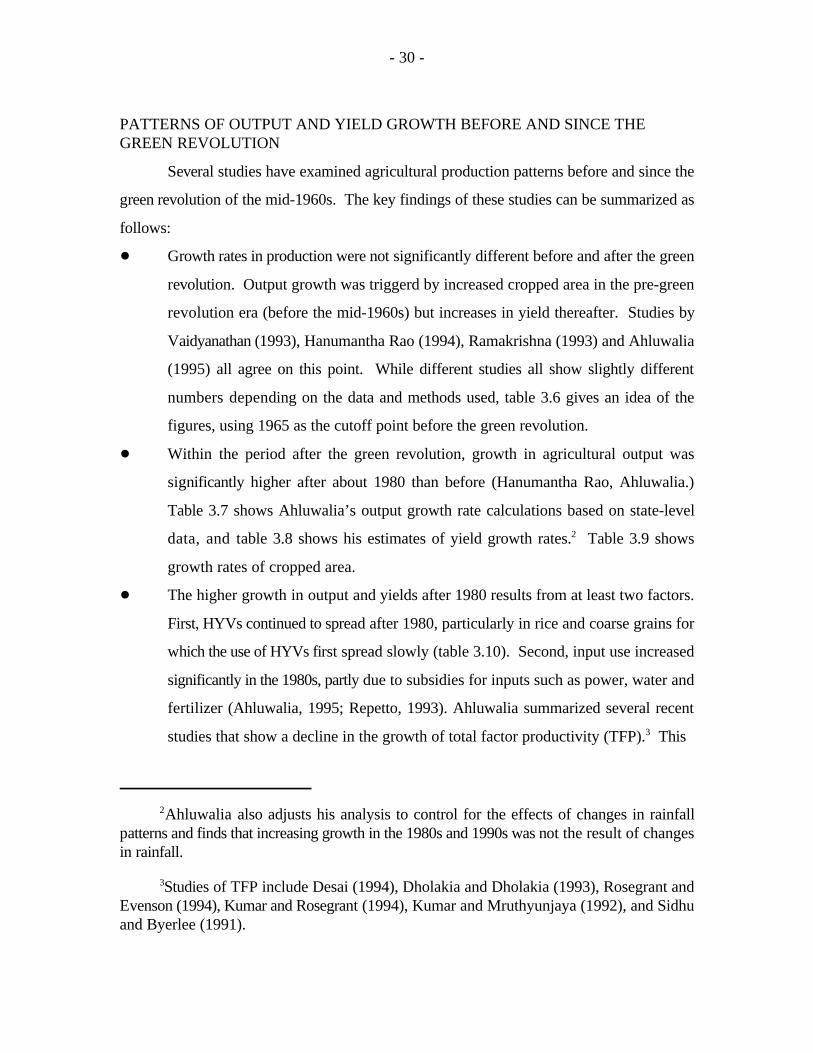
Ahluwalia also adjusts his analysis to control for the effects of changes in rainfall2
patterns and finds that increasing growth in the 1980s and 1990s was not the result of changesin rainfall.
Studies of TFP include Desai (1994), Dholakia and Dholakia (1993), Rosegrant and3
Evenson (1994), Kumar and Rosegrant (1994), Kumar and Mruthyunjaya (1992), and Sidhuand Byerlee (1991).
PATTERNS OF OUTPUT AND YIELD GROWTH BEFORE AND SINCE THEGREEN REVOLUTION
Several studies have examined agricultural production patterns before and since the
green revolution of the mid-1960s. The key findings of these studies can be summarized as
follows:
! Growth rates in production were not significantly different before and after the green
revolution. Output growth was triggerd by increased cropped area in the pre-green
revolution era (before the mid-1960s) but increases in yield thereafter. Studies by
Vaidyanathan (1993), Hanumantha Rao (1994), Ramakrishna (1993) and Ahluwalia
(1995) all agree on this point. While different studies all show slightly different
numbers depending on the data and methods used, table 3.6 gives an idea of the
figures, using 1965 as the cutoff point before the green revolution.
! Within the period after the green revolution, growth in agricultural output was
significantly higher after about 1980 than before (Hanumantha Rao, Ahluwalia.)
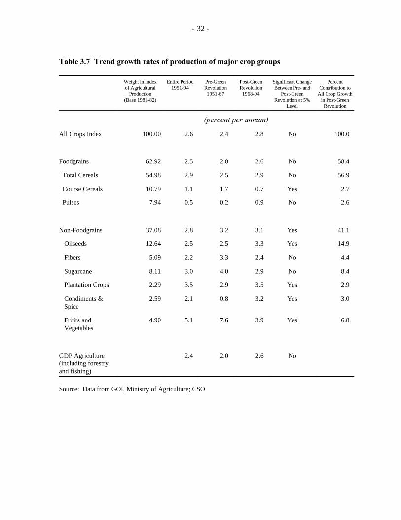
Table 3.7 shows Ahluwalia’s output growth rate calculations based on state-level
data, and table 3.8 shows his estimates of yield growth rates. Table 3.9 shows2
growth rates of cropped area.
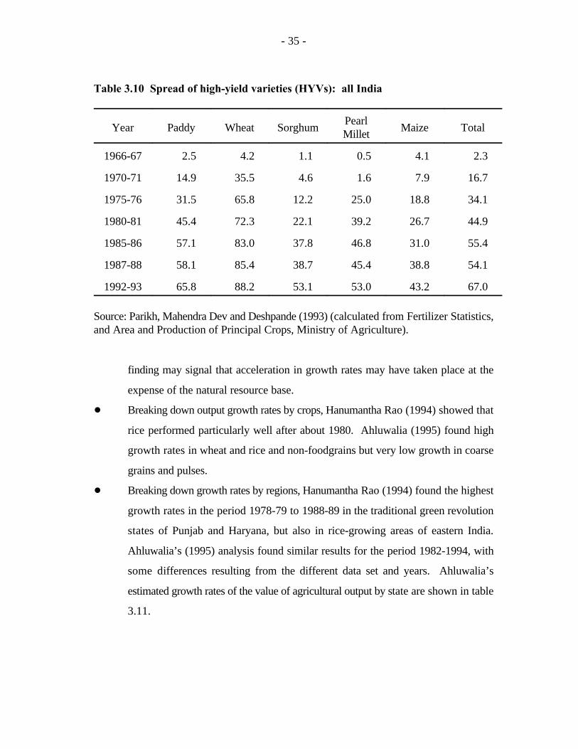
! The higher growth in output and yields after 1980 results from at least two factors.
First, HYVs continued to spread after 1980, particularly in rice and coarse grains for
which the use of HYVs first spread slowly (table 3.10). Second, input use increased
significantly in the 1980s, partly due to subsidies for inputs such as power, water and
fertilizer (Ahluwalia, 1995; Repetto, 1993). Ahluwalia summarized several recent
studies that show a decline in the growth of total factor productivity (TFP). This 3

- 31 -
Table 3.6 Annual growth in food grain production, area and productivity1950-51 to 1990-91
Food grains Non-food grains All crops Period Produc- Area Yield Produc- Area Yield Produc- Area Yield
tion tion tion
1950-51 to 2.58 1.24 1.32 3.41 2.18 1.20 2.75 1.43 1.311964-65
1967-68 to 2.80 0.20 2.60 2.82 0.54 2.27 02.82 0.27 2.531990-91
1950-51 to 2.71 0.55 2.16 2.76 0.91 1.75 2.69 0.63 2.051990-91
Source: Ramakrishna, 1993.
Note: Ramakrishna omits the severe drought years of 1965-66 and 1966-67 because as starting orending points in the analysis, they would move growth rates excessively downward or upward.
- 32 -
Table 3.7 Trend growth rates of production of major crop groups
Weight in Index Entire Period Pre-Green Post-Green Significant Change Percentof Agricultural 1951-94 Revolution Revolution Between Pre- and Contribution to
Production 1951-67 1968-94 Post-Green All Crop Growth(Base 1981-82) Revolution at 5% in Post-Green
Level Revolution
(percent per annum)
All Crops Index 100.00 2.6 2.4 2.8 No 100.0
Foodgrains 62.92 2.5 2.0 2.6 No 58.4
Total Cereals 54.98 2.9 2.5 2.9 No 56.9
Course Cereals 10.79 1.1 1.7 0.7 Yes 2.7
Pulses 7.94 0.5 0.2 0.9 No 2.6
Non-Foodgrains 37.08 2.8 3.2 3.1 Yes 41.1
Oilseeds 12.64 2.5 2.5 3.3 Yes 14.9
Fibers 5.09 2.2 3.3 2.4 No 4.4
Sugarcane 8.11 3.0 4.0 2.9 No 8.4
Plantation Crops 2.29 3.5 2.9 3.5 Yes 2.9
Condiments & 2.59 2.1 0.8 3.2 Yes 3.0 Spice
Fruits and 4.90 5.1 7.6 3.9 Yes 6.8 Vegetables
GDP Agriculture 2.4 2.0 2.6 No(including forestryand fishing)
Source: Data from GOI, Ministry of Agriculture; CSO

- 33 -
Table 3.8. Trend growth rates of yield of major crop groups
Weight in Post-Green Post-Green Post-Green SignificantIndex of Revolution Revolution Revolution Change
Agricultural 1968-94 Period-I Period-II BetweenProduction 1968-81 1982-94 Period I and
(Base Period II at1981-82) 5% Level
(percent per annum)
All Crops Index 100.00 2.0 1.3 2.5 Yes
Foodgrains 62.92 2.2 1.3 2.8 Yes
Total Cereals 54.98 2.4 1.7 2.9 Yes
Coarse Cereals 10.79 1.7 1.6 2.4 No
Pulses 7.94 0.7 -0.7 1.1 Yes
Non-Foodgrains 37.08 1.8 1.2 2.3 Yes
Oilseeds 12.64 1.6 0.5 2.3 Yes
Fibers 5.09 2.6 2.3 4.0 No
Sugarcane 8.11 1.3 0.8 1.5 No
Plantation Crops 2.29 1.8 2.3 2.2 No
Condiments & Spice 2.59 1.5 0.4 1.8 Yes
Fruits & Vegetables 4.90 1.9 2.0 2.0 No
Source: Data till 1991 from GOI, Ministry of Agriculture, ‘Area and Production ofPrincipal Crops in India 1990-93.’ Data from 1992-94 from Ministry of Agriculture

- 34 -
Table 3.9. Trend growth rates of area of major crop groups
Weight in Post-Green Post-Green Post-Green SignificantIndex of Revolution Revolution Revolution Change
Agricultural 1968-94 Period-I Period-II BetweenProduction 1968-81 1982-94 Period I and
(Base Period II at1981-82) 5% Level
(percent per annum)
All Crops Index 100.00 0.4 0.5 0.2 No
Foodgrains 62.92 0.1 0.4 -0.4 Yes
Total Cereals 54.98 0.1 0.4 -0.4 Yes
Coarse Cereals 10.79 -1.2 -1.0 -1.9 Yes
Pulses 7.94 0.2 0.4 -0.3 No
Non-Foodgrains 37.08 1.3 0.9 1.9 Yes
Oilseeds 12.64 1.2 0.3 2.6 Yes
Fibers 5.09 -0.3 0.2 -0.6 No
Sugarcane 8.11 1.6 1.8 1.4 No
Plantation Crops 2.29 2.2 2.5 2.2 Yes
Condiments & Spice 2.59 1.6 1.6 1.3 No
Fruits & Vegetables 4.90 1.7 2.3 1.4 Yes
Source: Data until 1991 from GOI, Ministry of Agriculture, ‘Area and Production ofPrincipal Crops in India 1990-93.’ Data from 1992-94 from Ministry of Agriculture.
- 35 -
Table 3.10 Spread of high-yield varieties (HYVs): all India
Year Paddy Wheat Sorghum Maize TotalPearlMillet
1966-67 2.5 4.2 1.1 0.5 4.1 2.3
1970-71 14.9 35.5 4.6 1.6 7.9 16.7
1975-76 31.5 65.8 12.2 25.0 18.8 34.1
1980-81 45.4 72.3 22.1 39.2 26.7 44.9
1985-86 57.1 83.0 37.8 46.8 31.0 55.4
1987-88 58.1 85.4 38.7 45.4 38.8 54.1
1992-93 65.8 88.2 53.1 53.0 43.2 67.0
Source: Parikh, Mahendra Dev and Deshpande (1993) (calculated from Fertilizer Statistics,and Area and Production of Principal Crops, Ministry of Agriculture).
finding may signal that acceleration in growth rates may have taken place at the
expense of the natural resource base.
! Breaking down output growth rates by crops, Hanumantha Rao (1994) showed that
rice performed particularly well after about 1980. Ahluwalia (1995) found high
growth rates in wheat and rice and non-foodgrains but very low growth in coarse
grains and pulses.
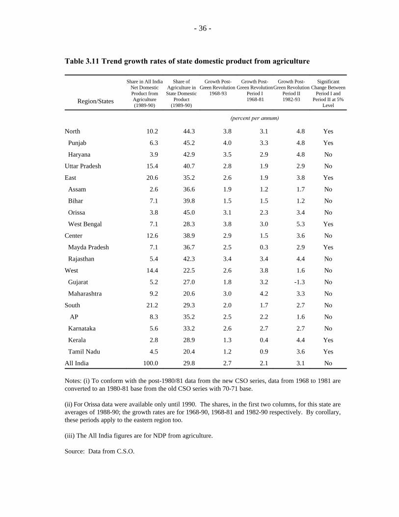
! Breaking down growth rates by regions, Hanumantha Rao (1994) found the highest
growth rates in the period 1978-79 to 1988-89 in the traditional green revolution
states of Punjab and Haryana, but also in rice-growing areas of eastern India.
Ahluwalia’s (1995) analysis found similar results for the period 1982-1994, with
some differences resulting from the different data set and years. Ahluwalia’s
estimated growth rates of the value of agricultural output by state are shown in table
3.11.
- 36 -
Table 3.11 Trend growth rates of state domestic product from agriculture
Region/States
Share in All India Share of Growth Post- Growth Post- Growth Post- SignificantNet Domestic Agriculture in Green Revolution Green RevolutionGreen Revolution Change BetweenProduct from State Domestic 1968-93 Period I Period II Period I andAgriculture Product 1968-81 1982-93 Period II at 5%(1989-90) (1989-90) Level
(percent per annum)
North 10.2 44.3 3.8 3.1 4.8 Yes
Punjab 6.3 45.2 4.0 3.3 4.8 Yes
Haryana 3.9 42.9 3.5 2.9 4.8 No
Uttar Pradesh 15.4 40.7 2.8 1.9 2.9 No
East 20.6 35.2 2.6 1.9 3.8 Yes
Assam 2.6 36.6 1.9 1.2 1.7 No
Bihar 7.1 39.8 1.5 1.5 1.2 No
Orissa 3.8 45.0 3.1 2.3 3.4 No
West Bengal 7.1 28.3 3.8 3.0 5.3 Yes
Center 12.6 38.9 2.9 1.5 3.6 No
Mayda Pradesh 7.1 36.7 2.5 0.3 2.9 Yes
Rajasthan 5.4 42.3 3.4 3.4 4.4 No
West 14.4 22.5 2.6 3.8 1.6 No
Gujarat 5.2 27.0 1.8 3.2 -1.3 No
Maharashtra 9.2 20.6 3.0 4.2 3.3 No
South 21.2 29.3 2.0 1.7 2.7 No
AP 8.3 35.2 2.5 2.2 1.6 No
Karnataka 5.6 33.2 2.6 2.7 2.7 No
Kerala 2.8 28.9 1.3 0.4 4.4 Yes
Tamil Nadu 4.5 20.4 1.2 0.9 3.6 Yes
All India 100.0 29.8 2.7 2.1 3.1 No
Notes: (i) To conform with the post-1980/81 data from the new CSO series, data from 1968 to 1981 areconverted to an 1980-81 base from the old CSO series with 70-71 base.
(ii) For Orissa data were available only until 1990. The shares, in the first two columns, for this state areaverages of 1988-90; the growth rates are for 1968-90, 1968-81 and 1982-90 respectively. By corollary,these periods apply to the eastern region too.
(iii) The All India figures are for NDP from agriculture.
Source: Data from C.S.O.

- 37 -
! Ahluwalia’s summary of studies of TFP suggest that the main sources of TFP
growth are agricultural research, education, extension, market infrastructure,
irrigation and mechanization.
4. GROWTH OF OUTPUT, YIELDS AND CROPPED AREA: A DISTRICT-LEVEL ANALYSIS
In this section we compare growth rates of value of output in irrigated and
unirrigated areas using district level data. The analysis in this section proceeds in two steps.
First, we conduct tabular analysis of the growth of value of output for irrigated and rainfed
districts of the five agroclimatic zones listed in table 2.3. This analysis is based on district
level data for 243 districts, the majority of the districts in the five zones. Figures are
presented for three different time periods to examine differences in summary performance
indicators over space and time. Second, we estimate a production function based on the
district level data. The production function follows ICAR’s agroecological zoning system;
of the 20 zones defined by ICAR, 15 are included in the area under study.
Based on the background information provided in the previous section, we expect
to find in the analysis the following trends. In the production function analysis, we expect
irrigation to make the greatest contribution to the value of output. In the tabular analysis
in which the years before, during and after the green revolution are examined separately,
we expect the trends to change as follows. In period 1, prior to the green revolution, we
expect rising growth rates to be driven by increases in both net and gross cropped area. Net
cropped area rises as more land is cleared for agriculture, and gross cropped area increases
with the spread of irrigation and multiple-cropping in dryland areas. In addition, irrigation
will raise crop yields somewhat even without the benefit of HYVs. In period 2, we expect
growth rates to be triggered by large yield increases in irrigated areas. In period 3, we
expect growth rates in irrigated areas to slow but growth rates in favorable rainfed areas
to rise. In periods 2 and 3 we do not expect much overall change in net cropped area,
though of course we do expect shifts in area from one crop to another.

- 38 -
Defining three subperiods in the study period of 1956-1991 necessarily is somewhat
arbitrary. Ideally the divisions would be based on changes in the factors expected to affect
growth in value of output, such as the spread of HYVs or irrigation. On the other hand,
easily observable changes in such variables may not exist. Other factors will also be
important when we calculate growth rates for each of the subperiods. For example, the
calculated growth rate may rise significantly if the first year of a subperiod is a drought year,
and it may fall if the last year is a drought year. As a result, working around drought years
is more important than identifying changes in trends in growth rates and HYV adoption.
The three subperiods defined in the study are 1956/57-1967/68, 1968/69-1979/80,
and 1980/81-1990/1991. The first period extends until 1968/69 even though 1965/66, the
year HYVs were introduced, would be a natural starting point for period 2. However,
1965/66 and 1966/67 were both severe drought years. If the last year of a period is a
drought year with unusually low output, the growth rate for the period as a whole will be
underestimated. Likewise, if the first year is a drought year, the growth rate for the whole
period will be overestimated. At the end of the first period, HYVs covered roughly 5% of
all area under cereals. At the end of the second period, HYVs covered nearly half of all
cereal area, and about three quarters of all wheat area. We expect that almost all of the
growth in HYVs in period 2 took place in irrigated areas, and much of that in period 3 took
place in rainfed areas. While the definition of subperiods may not perfectly capture changes
in the status of HYVs, it is acceptable.
An alternate approach would be to delete the two drought years, ending period 1
in 1964/65 and beginning period 2 in 1967/68. This is the same approach as used by Hazell
(1982), Hanumantha Rao (1994) and Ramakrishna (1993) in similar studies, cited above.
In fact, a number of reasonable divisions could have been devised, but none would be
perfect. It is important to note that every delineation of time periods will yield slightly
different results. The results reported below represent rough indications of the growth rates
in output, yield and cropped area for different regions and conditions and time periods in
the overall period under study, but they are not the last word. More detailed analysis will
be needed for more precise results.

- 39 -
Net cropped area and cropping intensity are the appropriate data for the analysis of all4
crops. For cereals and other crops, gross cropped area is sufficient and cropping intensitymay be omitted. “Output” refers to the value of output for the analysis of all crops and allcereals, but physical output is used for the analysis of individual crops.
TABULAR ANALYSIS OF GROWTH RATES IN VALUE OF OUTPUT
For the tabular analysis of the sources of growth of output, we group districts into
a total of ten categories, including five agroclimatic zones and two irrigation categories as
described in table 2.3. We conduct the analysis separately for all crops, all cereals, and
major cereal crops. The tables contain growth rates of value of output, yield, net cropped
area and cropping intensity. Note that because 4
production = net area x yield x cropping intensity , (a) (A) (Y) (C)
then
growth (a) = growth (A) + growth (Y) + growth (C).
The figures in the tables reflect this disaggregation, as the growth of output is
always the sum of the growth rates of the other three factors.
As explained in section 2, irrigated area grew steadily during the period under study,
so some districts changed from less than 25% area irrigated to greater than 25% area
irrigated. This is the case for 59 districts out of the 243 districts in the sample. To be as
precise as possible in defining rainfed and irrigated districts requires omitting these 59
districts from the analysis. On the other hand, doing so reduces the sample to 184 and thus
fails to utilize valuable data. As a result, the analysis is carried out twice, once with 184
districts and again with 243. We report both sets of results in order to demonstrate their
sensitivity to changes in specifications. The analysis based on 184 districts is more suitable
if our intention is to compare performance of districts with distinctly different irrigation
status, but the analysis based on 243 districts is more appropriate if we wish to examine
trends in the aggregate, because it uses more data.

- 40 -
All Crops
Table 4.1 shows the growth rate of value of output for all crops for the ten zones
and 3 subperiods. The calculations are based on the 184 districts whose irrigation status
is constant for the period under study. The most notable output of this analysis is that the
value of output grows steadily in each period, at rates of 1.75% in period 1, 2.69% in
period 2, and 3.56% in period 3. For all three periods taken together, overall output grew
at 2.37%; this overall growth was driven heavily by yield increases of 2.00% per year.
Rising yields are a key factor in each period examined separately; in periods 2 and 3,
increases in cropping intensity are also somewhat important. Increases in net cropped area
are small in the first period and zero or negative thereafter. These findings are consistent
with gradual increases in irrigation and adoption of HYVs and other inputs.
Examining the results by agroclimatic zone shows few interesting patterns. In
period 1, zone 2 (the eastern Gangetic plain) had the highest growth, followed by zones 1
(northwestern Indogangetic plain) and 3 (central/eastern highlands). In period 2, growth
was fastest in zone 4 (the central/western areas of Madhya Pradesh and Rajasthan plus most
of Gujarat), followed by zone 5, the south. In period 3, growth in value of output was high
in all zones. When these results are broken down to account for differences in irrigation,
the results change somewhat; irrigated areas of zone 1, the northwestern plains, has the
highest aggregate growth overall though not the highest growth in each period examined
separately.
Value of output and yields were generally higher in irrigated districts, but the
difference is not great. In zone 1, the northern Indo-Gangetic Plain, value of output and
yields were consistently higher in irrigated than dry districts for all three periods. This is
not surprising given the high proportion of area irrigated and the low rainfall. In zone 2,
the eastern Gangetic plain, and zone 3, the eastern and central highlands of Madhya
Pradesh, Orissa and southern Bihar, there was no clear pattern, with only small differences

- 41 -
Table 4.1 Growth rates of output, yield, net cropped area and cropping intensity: All crops
District All periods (1956-1990) Period 1 (1956-1965) Period 2 (1966-1979) Period 3 (1980-1990) Category
Compound Annual Growth (%)
Value of Cropping Value of Cropping Value of Cropping Value of Croppingoutput intensity output intensity output intensity output intensity
Yield cropped Yield cropped Yield cropped Yield croppedNet Net Net Net
area area area area
All districts(sample of
184)
2.37 2.01 -0.01 0.29 1.75 1.41 0.29 0.55 2.69 2.20 0.04 0.44 3.56 2.81 -0.25 0.38
All districts(sample of
243)
2.48 2.09 -0.01 0.32 2.07 1.63 0.36 0.07 2.65 2.19 0.01 0.43 3.69 2.97 -0.23 0.40
Disaggregated by Zones (sample of 184)
Zone 1,rainfed
2.50 2.03 0.26 0.20 1.69 1.52 0.31 -0.15 0.33 0.11 -0.02 0.23 1.69 1.25 0.24 0.19
Zone 1,irrigated
3.78 3.09 0.06 0.61 3.27 2.96 0.02 0.27 3.33 2.47 0.18 0.65 4.14 3.60 0.01 0.51
Zone 2,rainfed
2.19 1.07 0.09 0.57 4.54 3.52 1.07 -0.08 1.60 0.32 0.36 0.91 4.73 0.89 -0.36 0.65
Zone 2,irrigated
2.89 2.23 -0.11 0.45 4.37 3.40 0.73 0.20 2.42 1.89 0.04 0.49 4.82 1.76 -0.23 0.79
Zone 3,rainfed
2.14 1.53 0.39 0.21 2.02 1.17 0.91 -0.06 1.42 0.74 0.41 0.27 3.75 3.58 -0.19 0.35
Zone 3,irrigated
2.18 1.09 0.42 0.31 2.35 0.59 1.26 0.49 1.64 1.03 0.11 0.50 3.88 -1.15 1.41 0.87
Zone 4,rainfed
2.13 1.97 -0.13 0.29 0.63 0.57 0.07 -0.01 3.53 3.22 -0.13 0.43 2.96 3.27 -0.77 0.47
Zone 4,irrigated
2.58 1.67 0.37 0.52 0.44 -0.39 1.52 -0.68 3.06 2.35 -0.36 1.06 3.78 2.79 0.65 0.31
Zone 5,rainfed
2.47 2.67 -0.34 0.14 1.10 1.38 -0.42 0.15 3.07 2.86 0.03 0.17 4.22 3.42 0.54 0.24
Zone 5,irrigated
2.06 2.33 -0.16 -0.10 1.98 1.53 0.37 0.06 2.62 2.40 -0.09 0.30 3.19 2.57 0.34 0.27
- 42 -
between rainfed and irrigated performance. This is not very surprising given the high rainfall
in these two regions. Zone 4, the central and western highlands of Madhya Pradesh and
Rajasthan and most of Gujarat, had low growth in both irrigated and rainfed districts in period
1 but high growth in both thereafter. In Zone 5, covering most of the southern states of
Maharashtra, Andhra Pradesh and Karnataka, output and yield grew faster in irrigated areas
in period 1, but faster in rainfed areas in periods 2 and 3. We do not have an explanation for
this observed pattern.
As mentioned above, we also examine the results for all districts in the 450-1600 mm
rainfall range, including those whose irrigation status changed during the period under study.
This increases the number of districts from 184 to 243; the data are also shown in table 4.1.
The results for the period as a whole do not change much between the two samples, but for
some zones in some periods, the results do change significantly. As mentioned above, the
243-district sample is most useful for examining more aggregate results, so we are not
concerned about differences in the disaggregated results.
All Cereals
The data for cereals, not surprisingly, show results that are more consistent with what
we would expect based on our knowledge of changes in agricultural technology during the
period under study. Examining the data for both the 184-district and 243-district data sets
in table 4.2, growth in output and yields was highest in periods 2, the main green revolution
years, and period 3, when green revolution technology was still spreading for some crops in
some areas but cropped area was not growing as fast. Growth in output and yield was lowest
(but still significantly positive) in period 1. Cropped area under cereals also shows expected
results; it grew fastest in periods 1 and 2, when irrigation spread most rapidly, but it slowed
in period 3.
Examining the data for 184 districts by zone, the fastest growth in value of output for
any zone in any period comes in periods 2 in irrigated areas of zone 1, the main green
revolution areas of Punjab, Haryana and Western UP, and in zone 2, the eastern Gangetic
plains, in period 3. Zone 2 performs well in all periods; interestingly, its growth is driven
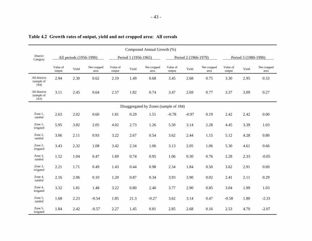
- 43 -
Table 4.2 Growth rates of output, yield and net cropped area: All cereals
DistrictCategory
Compound Annual Growth (%)
All periods (1956-1990) Period 1 (1956-1965) Period 2 (1966-1979) Period 3 (1980-1990)
Value of Net cropped Value of Net cropped Value of Net cropped Value of Net croppedoutput area output area output area output areaYield Yield Yield Yield
All districts(sample of
184)
2.94 2.30 0.62 2.19 1.49 0.68 3.45 2.68 0.75 3.30 2.95 0.33
All districts(sample of
243)
3.11 2.45 0.64 2.57 1.82 0.74 3.47 2.69 0.77 3.37 3.09 0.27
Disaggregated by Zones (sample of 184)
Zone 1,rainfed
2.63 2.02 0.60 1.81 0.29 1.51 -0.78 -0.97 0.19 2.42 2.42 0.00
Zone 1,irrigated
5.95 3.82 2.05 4.02 2.73 1.26 5.50 3.14 2.28 4.45 3.39 1.03
Zone 2,rainfed
3.06 2.11 0.93 3.22 2.67 0.54 3.62 2.44 1.15 5.12 4.28 0.80
Zone 2,irrigated
3.43 2.32 1.08 3.42 2.34 1.06 3.13 2.05 1.06 5.30 4.61 0.66
Zone 3,rainfed
1.52 1.04 0.47 1.69 0.74 0.95 1.06 0.30 0.76 2.28 2.33 -0.05
Zone 3,irrigated
2.21 1.71 0.49 1.43 0.44 0.98 2.34 1.84 0.50 3.62 2.91 0.69
Zone 4,rainfed
2.16 2.06 0.10 1.20 0.87 0.34 3.93 3.90 0.02 2.41 2.11 0.29
Zone 4,irrigated
3.32 1.81 1.48 3.22 0.80 2.40 3.77 2.90 0.85 3.04 1.99 1.03
Zone 5,rainfed
1.68 2.23 -0.54 1.85 21.3 -0.27 3.62 3.14 0.47 -0.58 1.80 -2.33
Zone 5,irrigated
1.84 2.42 -0.57 2.27 1.45 0.81 2.85 2.68 0.16 2.53 4.70 -2.07

- 44 -
mainly by yield increases but also by increases in cropped area. Very high growth rates of
output are also found in period 1 in irrigated areas of zones 2 and 4, in period 2 in rainfed
areas of zone 5 and both rainfed and irrigated districts of zones 2 and 4. Zone 3 (the central
eastern plateau) performs poorly in period 1, better in irrigated areas in period 2, and fairly
well in period 3 as yield grew fairly rapidly.
Individual Cereals
In this section we examine the data for 5 individual cereal crops: wheat, rice, maize,
sorghum (jowar) and pearl millet (bajra). Output is measured in tons rather than prices, since
physical units are comparable within a given crop.
Wheat shows the most consistently high growth rates of any crop (table 4.3). In the
aggregate (for the data based on both 184 and 243 districts), output growth and yield growth
were high in period one but even higher in periods 2 and 3. These results are consistent with
those of Byerlee (1992), who found rapid growth in wheat yields even after HYVs accounted
for the vast majority of wheat acreage.
Looking at individual zones for the 184 district data set, growth in output in period
1, prior to the introduction of HYVs, was centered in irrigated areas of zone 1 (the
northwest) and both rainfed and irrigated districts of zone 2 (the east). In period 2, these
areas continued to have high growth in output but were also joined by irrigated districts of
zone 3 (central/eastern India), both irrigated and rainfed districts of zone 4 (central/western
India), and rainfed districts of zone 5 (the south). Most of these high growth rates in output
continued in period 3, with the notable exception of rainfed areas of zone 5 (the south), where
output fell precipitously. This is only a very minor wheat growing area, so swings in output
will have little impact on nationwide performance. In all three periods, growth in output was
stimulated by a combination of increases in both yield and cropped area.
Rice also performed well (table 4.4), but not to the same extent as wheat. Examining
the aggregate data from 184 districts, growth in value is significantly positive for all three
periods; it is highest in the green revolution years of period 2 and lowest in period 3.
Interestingly, period 3 shows the highest growth in rice yields, but these are more than

- 45 -
Table 4.3 Growth rates of output, yield and cropped area: Wheat
DistrictCategory
Compound Annual Growth (%)
All periods (1956-1990) Period 1 (1956-1965) Period 2 (1966-1979) Period 3 (1980-1990)
Value of Net cropped Value of Net cropped Value of Net cropped Value of Net croppedoutput area output area output area output areaYield Yield Yield Yield
All districts(sample of
184)
5.81 3.50 2.23 3.74 2.84 0.88 4.81 2.39 2.36 6.29 5.07 1.16
All districts(sample of
243)
5.85 3.53 2.25 3.07 2.50 0.55 5.23 2.60 2.56 5.60 4.41 1.13
Disaggregated by Zones (sample of 184)
Zone 1,rainfed
3.14 1.87 1.24 -0.59 -1.32 0.74 0.02 -0.96 0.99 1.86 2.03 -0.16
Zone 1,irrigated
6.31 3.51 2.70 5.07 3.52 1.50 5.22 2.22 2.93 3.86 2.99 0.84
Zone 2,rainfed
6.96 4.07 2.78 10.07 9.89 0.16 6.13 3.28 2.76 6.09 1.12 4.91
Zone 2,irrigated
6.96 3.57 3.27 7.40 3.80 3.47 5.58 3.31 2.20 5.69 3.80 1.82
Zone 3,rainfed
2.20 1.83 0.37 1.65 1.54 0.11 2.07 1.37 0.69 4.12 3.68 0.42
Zone 3,irrigated
6.15 3.44 2.61 2.95 1.20 1.73 5.50 3.56 1.87 8.66 5.76 2.74
Zone 4,rainfed
2.68 2.83 -0.14 0.65 1.89 -1.22 4.10 2.39 1.70 12.78 14.46 -1.47
Zone 4,irrigated
5.36 2.56 2.72 -1.73 -0.92 -0.82 9.06 2.79 6.09 2.66 2.99 -0.32
Zone 5,rainfed
0.61 -0.48 1.36 -1.25 1.93 -2.97 11.19 5.38 5.77 -19.45 -25.70 8.06
Zone 5,irrigated
-0.15 0.13 -0.06 0.61 0.26 0.05 -0.68 0.00 -0.32 -1.83 -0.17 -0.28
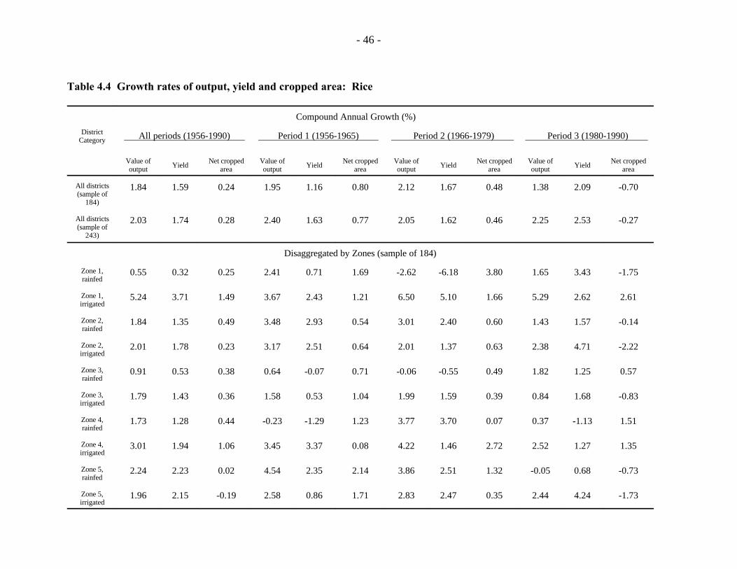
- 46 -
Table 4.4 Growth rates of output, yield and cropped area: Rice
DistrictCategory
Compound Annual Growth (%)
All periods (1956-1990) Period 1 (1956-1965) Period 2 (1966-1979) Period 3 (1980-1990)
Value of Net cropped Value of Net cropped Value of Net cropped Value of Net croppedoutput area output area output area output areaYield Yield Yield Yield
All districts(sample of
184)
1.84 1.59 0.24 1.95 1.16 0.80 2.12 1.67 0.48 1.38 2.09 -0.70
All districts(sample of
243)
2.03 1.74 0.28 2.40 1.63 0.77 2.05 1.62 0.46 2.25 2.53 -0.27
Disaggregated by Zones (sample of 184)
Zone 1,rainfed
0.55 0.32 0.25 2.41 0.71 1.69 -2.62 -6.18 3.80 1.65 3.43 -1.75
Zone 1,irrigated
5.24 3.71 1.49 3.67 2.43 1.21 6.50 5.10 1.66 5.29 2.62 2.61
Zone 2,rainfed
1.84 1.35 0.49 3.48 2.93 0.54 3.01 2.40 0.60 1.43 1.57 -0.14
Zone 2,irrigated
2.01 1.78 0.23 3.17 2.51 0.64 2.01 1.37 0.63 2.38 4.71 -2.22
Zone 3,rainfed
0.91 0.53 0.38 0.64 -0.07 0.71 -0.06 -0.55 0.49 1.82 1.25 0.57
Zone 3,irrigated
1.79 1.43 0.36 1.58 0.53 1.04 1.99 1.59 0.39 0.84 1.68 -0.83
Zone 4,rainfed
1.73 1.28 0.44 -0.23 -1.29 1.23 3.77 3.70 0.07 0.37 -1.13 1.51
Zone 4,irrigated
3.01 1.94 1.06 3.45 3.37 0.08 4.22 1.46 2.72 2.52 1.27 1.35
Zone 5,rainfed
2.24 2.23 0.02 4.54 2.35 2.14 3.86 2.51 1.32 -0.05 0.68 -0.73
Zone 5,irrigated
1.96 2.15 -0.19 2.58 0.86 1.71 2.83 2.47 0.35 2.44 4.24 -1.73

- 47 -
counterbalanced by a drop in cropped area. In the data for all 243 districts, periods 2 and 3
reverse order in the ranking of overall output growth rates, while the yield and cropped area
findings do not change. This shows that the rankings are not very robust; in fact, in the data
for 243 districts, the three periods show nearly identical performance in growth of output.
For aggregate data in which we are not concerned about changes in irrigated area, the 243
district sample is more reliable because it contains more observations.
Examining the data by zone using the 184 district sample, irrigated districts in zone
1 (the northwest) consistently show the highest growth. In period 2 this comes from rapidly
increasing yields, but in period 3 it is evenly divided between yield and area growth. Notably,
performance in output and yield are very poor in rainfed areas of zone 1 in period 2, the green
revolution years. There is not much evidence of the rapid growth in rice output in eastern
India, mentioned above, though yields do rise substantially in irrigated areas of zone 2 in
period 3. On the other hand, cropped area drops greatly in this zone during the same time
period. Output and yield are also high in irrigated districts of zones 4 and 5, which are mainly
along the coast of the Bay of Bengal. With a few exceptions, performance is generally better
in predominantly irrigated than predominantly rainfed districts. We do not have an
explanation for the lack of evidence of growth in rainfed rice in recent years.
There are a few notable differences between the results for the data for 243 districts
vs 184 districts. In particular, output and yield performed extremely well in rainfed districts
of zone 1 in period 3 when all 243 districts are analyzed. Also, the poor performance for this
zone in period 2 is not found when all 243 districts are examined.
Maize shows the surprising pattern of low growth in output and yields during the
green revolution years of period 2, but high growth in periods 1 and 3 (table 4.5). Yields
grew at a fast rate in period one only, while cropped area grew at reasonably high rates in
periods 1 and 3. One explanation for this pattern may lie in table 3.10, which shows that
HYVs spread more slowly for maize than other crops. By 1984, only 33% of maize was
under HYVs compared with 52% for rice and 81% for wheat. Yield growth in period one
may have come from increases in irrigated area. The negative yield growth in period 2 is
puzzling, however, as percent area under HYVs grew from 6% to 33%. Yields rebounded
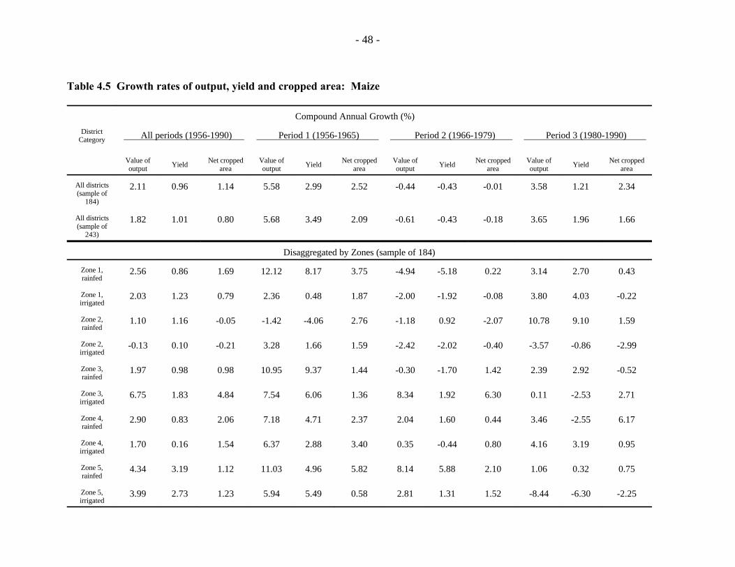
- 48 -
Table 4.5 Growth rates of output, yield and cropped area: Maize
DistrictCategory
Compound Annual Growth (%)
All periods (1956-1990) Period 1 (1956-1965) Period 2 (1966-1979) Period 3 (1980-1990)
Value of Net cropped Value of Net cropped Value of Net cropped Value of Net croppedoutput area output area output area output areaYield Yield Yield Yield
All districts(sample of
184)
2.11 0.96 1.14 5.58 2.99 2.52 -0.44 -0.43 -0.01 3.58 1.21 2.34
All districts(sample of
243)
1.82 1.01 0.80 5.68 3.49 2.09 -0.61 -0.43 -0.18 3.65 1.96 1.66
Disaggregated by Zones (sample of 184)
Zone 1,rainfed
2.56 0.86 1.69 12.12 8.17 3.75 -4.94 -5.18 0.22 3.14 2.70 0.43
Zone 1,irrigated
2.03 1.23 0.79 2.36 0.48 1.87 -2.00 -1.92 -0.08 3.80 4.03 -0.22
Zone 2,rainfed
1.10 1.16 -0.05 -1.42 -4.06 2.76 -1.18 0.92 -2.07 10.78 9.10 1.59
Zone 2,irrigated
-0.13 0.10 -0.21 3.28 1.66 1.59 -2.42 -2.02 -0.40 -3.57 -0.86 -2.99
Zone 3,rainfed
1.97 0.98 0.98 10.95 9.37 1.44 -0.30 -1.70 1.42 2.39 2.92 -0.52
Zone 3,irrigated
6.75 1.83 4.84 7.54 6.06 1.36 8.34 1.92 6.30 0.11 -2.53 2.71
Zone 4,rainfed
2.90 0.83 2.06 7.18 4.71 2.37 2.04 1.60 0.44 3.46 -2.55 6.17
Zone 4,irrigated
1.70 0.16 1.54 6.37 2.88 3.40 0.35 -0.44 0.80 4.16 3.19 0.95
Zone 5,rainfed
4.34 3.19 1.12 11.03 4.96 5.82 8.14 5.88 2.10 1.06 0.32 0.75
Zone 5,irrigated
3.99 2.73 1.23 5.94 5.49 0.58 2.81 1.31 1.52 -8.44 -6.30 -2.25

- 49 -
in period three to significantly positive, if not high rates. The results are robust between the
184 and 243 district data sets.
Examining the data by district, output grew at very high rates in period 1 in several
zones; they were highest in rainfed areas of zones 1 (the northwest), 3 (the eastern central
highlands) and 5 (the south), but irrigated zones also experienced rapid growth. Yields
followed a similar pattern, and net cropped area increased significantly in most zones. In
period 2, most zones experienced negative yield growth, with the exception of rainfed areas
of zone 5, where it continued to grow rapidly. Irrigated areas of zone 3 and rainfed areas of
zone 5 continued to show very high growth rates in output in period 2. In period 3,
performance was strong in many zones. Growth in output stemmed from yield growth in
some districts but area increases in others. Only irrigated areas of zone 5 performed poorly,
a result of rapid declines in both yield and area. The results for maize are mainly robust
between data sets, but there are some exceptions.
Sorghum (jowar) grew rapidly in both output and yields -- both over 3% per year --
in period 2, the green revolution years, followed by smaller increases of about 1.5% in period
3 (table 4.6). Cropped area showed practically no growth in these periods, however. This
pattern is consistent with the view of sorghum as an inferior crop that will not realize
increased net cropped area in response to increases in yield. In the pre-green revolution years
of period 1, on the other hand, yield was stagnant but increases in net cropped area drove
modest increases in output. These patterns are all insensitive to changes in the data set.
Disaggregating the data does not reveal consistent patterns. Most zones show
negative trends in net cropped area throughout the period; these are counterbalanced by a few
zones with positive growth. In period 1, only rainfed districts of zones 1 (the northwest), 3
(the eastern central highlands) and 5 (the south) show positive growth in area, but of these,
only zone 3 has positive yield growth. Only the irrigated districts of zone 4 (the western
central areas) had high increases in yield, but these were more than offset by a reduction in
area. Only one district had more than 1% annual growth in output. These findings are
roughly constant for both data sets.

- 50 -
Table 4.6 Growth rates of output, yield and cropped area: Jowar (Sorghum)
DistrictCategory
Compound Annual Growth (%)
All periods (1956-1990) Period 1 (1956-1965) Period 2 (1966-1979) Period 3 (1980-1990)
Value of Net cropped Value of Net cropped Value of Net cropped Value of Net croppedoutput area output area output area output areaYield Yield Yield Yield
All districts(sample of
184)
1.51 1.53 0.00 0.82 -0.03 0.90 3.17 3.15 0.03 1.48 1.53 0.12
All districts(sample of
243)
1.38 1.47 -0.06 0.94 0.09 0.89 2.91 3.00 -0.08 1.27 1.48 -0.05
Disaggregated by Zones (sample of 184)
Zone 1,rainfed
-0.06 0.22 -0.28 -1.26 -2.70 1.48 -4.62 -4.25 -0.39 0.63 1.39 -0.75
Zone 1,irrigated
0.06 2.51 -2.38 -3.05 -2.69 -0.37 -2.07 0.75 -2.79 5.88 4.35 1.50
Zone 2,rainfed
-0.04 0.12 -0.19 0.58 0.66 -0.08 -0.20 -0.03 -0.17 1.54 0.80 0.42
Zone 2,irrigated
0.76 0.33 1.18 0.78 1.27 -0.48 0.66 0.19 0.47 2.11 0.30 8.63
Zone 3,rainfed
0.69 1.11 -0.42 2.18 1.03 1.14 -0.16 0.86 -1.01 -0.88 2.68 -3.48
Zone 3,irrigated
-0.83 0.36 -1.18 -2.80 -1.89 -0.93 -0.72 1.23 -1.93 -3.82 0.11 -3.93
Zone 4,rainfed
1.58 1.65 -0.01 0.90 -0.11 1.02 3.79 3.86 -0.07 1.44 1.38 0.28
Zone 4,irrigated
0.65 0.92 -0.43 -0.94 3.17 -0.01 0.42 2.56 -1.86 1.07 1.10 -0.03
Zone 5,rainfed
0.73 1.48 -0.75 -0.97 -0.12 -0.86 3.10 3.25 -0.15 -1.76 1.05 -2.79
Zone 5,irrigated
0.31 1.50 -1.18 0.17 0.62 -0.45 2.24 2.44 -0.19 1.19 4.00 -2.70
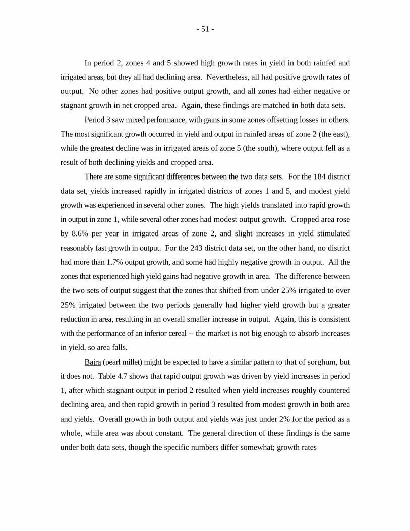
- 51 -
In period 2, zones 4 and 5 showed high growth rates in yield in both rainfed and
irrigated areas, but they all had declining area. Nevertheless, all had positive growth rates of
output. No other zones had positive output growth, and all zones had either negative or
stagnant growth in net cropped area. Again, these findings are matched in both data sets.
Period 3 saw mixed performance, with gains in some zones offsetting losses in others.
The most significant growth occurred in yield and output in rainfed areas of zone 2 (the east),
while the greatest decline was in irrigated areas of zone 5 (the south), where output fell as a
result of both declining yields and cropped area.
There are some significant differences between the two data sets. For the 184 district
data set, yields increased rapidly in irrigated districts of zones 1 and 5, and modest yield
growth was experienced in several other zones. The high yields translated into rapid growth
in output in zone 1, while several other zones had modest output growth. Cropped area rose
by 8.6% per year in irrigated areas of zone 2, and slight increases in yield stimulated
reasonably fast growth in output. For the 243 district data set, on the other hand, no district
had more than 1.7% output growth, and some had highly negative growth in output. All the
zones that experienced high yield gains had negative growth in area. The difference between
the two sets of output suggest that the zones that shifted from under 25% irrigated to over
25% irrigated between the two periods generally had higher yield growth but a greater
reduction in area, resulting in an overall smaller increase in output. Again, this is consistent
with the performance of an inferior cereal -- the market is not big enough to absorb increases
in yield, so area falls.
Bajra (pearl millet) might be expected to have a similar pattern to that of sorghum, but
it does not. Table 4.7 shows that rapid output growth was driven by yield increases in period
1, after which stagnant output in period 2 resulted when yield increases roughly countered
declining area, and then rapid growth in period 3 resulted from modest growth in both area
and yields. Overall growth in both output and yields was just under 2% for the period as a
whole, while area was about constant. The general direction of these findings is the same
under both data sets, though the specific numbers differ somewhat; growth rates

- 52 -
Table 4.7 Growth rates of output, yield and cropped area: Bajra (Millet)
DistrictCategory
Compound Annual Growth (%)
All periods (1956-1990) Period 1 (1956-1965) Period 2 (1966-1979) Period 3 (1980-1990)
Value of Net cropped Value of Net cropped Value of Net cropped Value of Net croppedoutput area output area output area output areaYield Yield Yield Yield
All districts(sample of
184)
1.92 1.83 0.09 1.04 2.10 -1.04 -0.13 1.25 -1.36 3.52 1.91 1.63
All districts(sample of
243)
2.10 1.95 0.15 3.10 3.32 -0.21 0.05 1.29 -1.22 2.53 1.58 0.97
Disaggregated by Zones (sample of 184)
Zone 1,rainfed
1.48 1.18 0.30 9.07 6.22 2.68 -6.05 -4.30 -1.83 6.91 4.56 2.26
Zone 1,irrigated
2.16 2.21 -0.05 0.81 2.02 -1.19 -0.67 -1.85 1.20 0.45 3.91 -3.32
Zone 2,rainfed
-0.28 0.20 -0.48 -0.27 0.41 -0.67 0.06 0.22 -0.16 -2.74 -0.31 -2.43
Zone 2,irrigated
1.29 0.12 1.17 1.63 1.59 0.03 -0.56 -0.10 -0.46 5.57 0.03 5.54
Zone 3,rainfed
0.97 0.55 0.46 -0.87 -2.05 1.37 -0.27 -0.27 0.38 -0.69 -0.50 -0.22
Zone 3,irrigated
0.74 1.10 -0.36 2.07 0.97 1.10 2.93 2.33 0.59 -6.46 -2.09 -4.47
Zone 4,rainfed
1.99 2.16 -0.15 0.14 1.99 -1.82 0.87 2.44 -1.53 2.72 1.70 1.07
Zone 4,irrigated
3.05 1.60 1.43 10.36 3.96 6.15 -2.57 -0.68 -1.93 10.60 6.38 3.97
Zone 5,rainfed
-2.13 0.42 -2.54 -3.27 -0.21 -3.07 -1.50 -0.97 -0.53 -4.87 1.33 -6.12
Zone 5,irrigated
0.73 2.13 -1.36 -0.65 1.40 -2.03 2.18 3.42 -1.19 1.76 2.65 -0.87

- 53 -
are significantly higher in period 1 but significantly lower in period 3 when all 243 districts
are analyzed, and overall growth rates are slightly higher.
Positive growth in output in period 1 resulted from a mixture of increases and declines
in area and yield in different zones. Three zones had an increase in both: these include rainfed
districts of zone 1 (the northwest), irrigated districts of zone 3 (the central/eastern highlands),
and irrigated districts of zone 4 (the western/central areas). Zones 1 and 4 had very rapid
output growth. Several other zones had yield and area moving in opposite directions, and
rainfed areas of zone 5 (the south) had negative growth in area, yield and output. These
patterns are largely duplicated in the data for 243 districts, though output changes from
stagnant to 2% growth in rainfed areas of zone 4.
In period 2, irrigated districts of zones 3 and 5 show positive growth in output, but
other zones have either negative or stagnant output. Most districts either declined in both
yield and area or one or the other. Rainfed areas of zone 1 showed a very sharp drop in yields
and output. These findings are roughly constant across data sets.
In period 3, the poor performance of rainfed areas of zone 1 were completely
reversed, with rapid growth in yield, area and output. High output growth in irrigated areas
of zone 2 is driven by area increases, and output growth in irrigated areas of zone 4 is driven
by growth in both area and yield. Most zones show rapid yield growth, while growth in
cropped area is significantly positive in some areas but significantly negative in others. These
findings are qualitatively the same in both data sets, but magnitudes of some indicators change
significantly between one district and another. Irrigated districts of zone 4, for example, show
only 2.3% growth in output in period 4 in the 243 district data set compared to 10.6% in the
184 district data set.
Summary Comments on the Tabular Analysis
Growth rates of the value of output, yield, cropped area and cropping intensities
provide an indication of the pattern of agricultural growth under different conditions in India.
On the whole, the findings reflect our prior expectations; for example, irrigated areas in zone
1, the northwestern green revolution belt, consistently show the highest growth rates in yield

- 54 -
and output, particularly in periods 2 and 3. Contrary to our expectations, we did not find
much evidence of exceptional rice and sorghum growth in period 3 in favorable rainfed areas
eastern and central India. However, in most zones for most crops, output and yield in
predominantly rainfed districts grew quite rapidly, nearly as much as in irrigated zones. This
suggests that rainfed agriculture has performed quite well, even if not up to the high standards
set by the performance of irrigated agriculture.
It is important to reiterate that the findings of the tabular analysis are more indicative
than definitive of trends in irrigated and rainfed agriculture in different agroecological zones
of India. As mentioned above, sensitivity of the calculated growth rates to specification of the
time periods and zones requires that we treat these results with caution. More precise
understanding requires a more detailed analysis that could not be undertaken with the
resources available for this study.
PRODUCTION FUNCTION ANALYSIS OF SOURCES OF GROWTH INPRODUCTIVITY
We use the district data to estimate a production function for Indian agriculture. As
mentioned earlier, the data cover 243 districts, or most of those in the Indo-Gangetic plains
and peninsular India with an average annual rainfall between 450 mm and 1600 mm. Those
with desert conditions (as in Western Rajasthan) or very high rainfall (as in the Western
Ghats) are excluded, since their conditions are not comparable to those in the rest of the
sampled districts.
The production function approach has some important advantages over tabular
analysis. First, there is no need to define districts as either irrigated or dry; instead, each
district is associated with a continuous variable indicating the percent irrigated area. Second,
there is no need to divide the sample into subperiods. Third, we can classify districts into
disaggregated agroclimatic zones without encountering presentation difficulties, as each zone
simply adds an additional line to the output. The data provide us with sufficient degrees
freedom and enough districts in each zone to categorize all districts according to ICAR’s 20-
- 55 -
See section 2 for a listing of the 20 zones. Many districts straddle two zones, in which5
case we put them in the zone in which most of the district lies. Coastal districts in TamilNadu, Orissa and Andhra Pradesh lie partially in zone 18 and partly in adjoining zones 7, 8,12 and 15; in this categorization they are all placed in the adjoining zones. Zone 3 is excludedfrom the production function analysis because it contains only one full district; others areplaced in adjoining zones.
zone system. The zones included in our sample are 2, 4, 5, 6, 7, 8, 9, 10, 11, 12, 13, and 15,
for a total of 12 of the 20 zones.5
The production function is a Cobb-Douglas type in which the coefficients represent
elasticities; the dependent variable is the value of output. Most of the variables in the
production function are self-explanatory. They are listed in table 4.8.
Prices in the analysis are taken as the average of prices prevailing over the overall
period under study. Constant prices are taken to avoid terms of trade effects that change
during the course of the study period. In a subsequent analysis a more sophisticated method
will be used to deflate prices over the course of the study period, but the system used here is
sufficient for our purpose, which is to obtain a preliminary understanding of the contribution
of various factors to agricultural production.
The estimated production function for 243 districts is presented in table 4.9. The
model’s explanatory power is reasonably high. All variables except the logarithm of literacy
and the dummy variables for zones 10 and 11 are significant at the 10% confidence level; the
remainder are all significant at the 1% confidence level.
On the whole, the elasticities are quite small, in most cases less than 0.15%. The
regression coefficients sum to about 1.15, suggesting the presence of economies of scale. The
variables with the highest values are gross cropped area, percent irrigated area, rainfall, labor,
tractors, and several of the zone dummies. Most of these results are not surprising; in a
country where water is scarce in most places most of the year, it makes sense that rainfall and
irrigation have a large impact on value of production. Gross cropped area has the largest
coefficient because the dependent variable is the total value of output, not the value of output
per hectare. The positive zone dummies are also to be expected, because the base zone is 2,
on the fringe of the Rajasthan desert where output is expected to be low. The
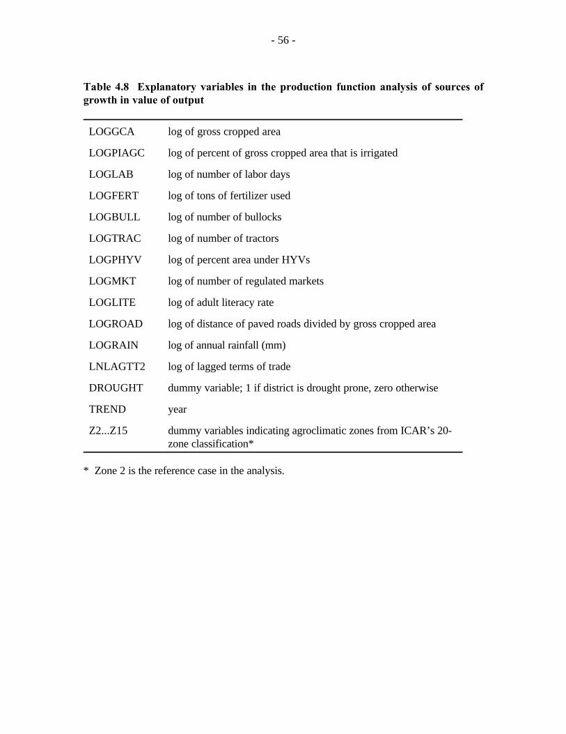
- 56 -
Table 4.8 Explanatory variables in the production function analysis of sources ofgrowth in value of output
LOGGCA log of gross cropped area
LOGPIAGC log of percent of gross cropped area that is irrigated
LOGLAB log of number of labor days
LOGFERT log of tons of fertilizer used
LOGBULL log of number of bullocks
LOGTRAC log of number of tractors
LOGPHYV log of percent area under HYVs
LOGMKT log of number of regulated markets
LOGLITE log of adult literacy rate
LOGROAD log of distance of paved roads divided by gross cropped area
LOGRAIN log of annual rainfall (mm)
LNLAGTT2 log of lagged terms of trade
DROUGHT dummy variable; 1 if district is drought prone, zero otherwise
TREND year
Z2...Z15 dummy variables indicating agroclimatic zones from ICAR’s 20-zone classification*
* Zone 2 is the reference case in the analysis.

- 57 -
Table 4.9 Coefficients of the production function variables
Variable Coeffecient
INTERCEP -1.77* (0.174)
LOGGCA 0.72* (0.014)
LOGPIAGC 0.13* (0.016)
LOGLAB 0.12* (0.014)
LOGFERT 0.05* (0.004)
LOGBULL 0.01* (0.003)
LOGTRAC 0.12* (0.004)
LOGPHYV 0.02* (0.004)
LOGMKT -0.02* (0.005)
LOGLITE -0.01 (0.015)
LOGROAD 0.03* (0.009)
LOGRAIN 0.16* (0.013)
LNLAGTT2 0.09* (0.017)
DROUGHT 0.07* (0.010)
TREND 0.01* (0.001)
Z4 0.25* (0.032)
Z5 0.32* (0.033)
Z6 0.14* (0.035)
Z7 0.14* (0.037)
Z8 0.30* (0.038)
Z9 0.28* (0.036)
Z10 0.05 (0.034)
Z11 0.01 (0.039)
Z12 0.37* (0.036)
Z13 0.16* (0.040)
Z15 1.26* (0.042)
R-square = 0.77Note: Standard errors in parentheses

- 58 -
strong positive contribution of tractors is not entirely straightforward. It may in fact reflect
the importance of overcoming power constraints in land preparation. A possible alternative
is that tractors act as a proxy for other variables related to infrastructure and capital that
contribute positively to the value of output. Yet another possibility is that tractors may be
highly collinear with bullocks and labor, two other variables that represent a “horsepower”
input. If so, tractors may simply capture much of the effect resulting from those two
variables. This would be consistent with the strong positive contribution of labor.
The significantly negative value of the coefficient for markets is puzzling, as is the
negative but insignificant coefficient for literacy. The negative coefficient for markets
represents the direct effect of the number of government regulated markets on output.
However, there may also be indirect effects that this analysis does not attempt to identify; for
example, markets may increase input use, thus increasing production indirectly despite the
negative direct effect in the production function estimation. More detailed analysis is needed
to fully explain the counterintuitive result shown here. A simultaneous equations model
would be needed to capture any possible indirect effects and eliminate endogeneity.
The negative value of the lagged terms of trade is also somewhat difficult to explain.
This finding suggests that the value of agricultural output declines after agricultural prices rise
relative to nonagricultural prices. A reasonable explanation for this result would be that
demand declines in response to higher prices, thus reducing the value of output in the
subsequent period. However, agricultural supply is relatively inelastic, and terms of trade
generally do not move very much over time (Hazell et al 1995). A possible alternate
explanation of the negative coefficient of the terms of trade would be reverse causality: that
terms of trade respond negatively to changes in output, which would make sense. Yet
another alternate explanation is the same as that for the negative coefficient for markets,
explained above: terms of trade may have a negative direct effect on the value of output, but
a positive indirect effect through positive effects on input use. Higher terms of trade would
reduce the price of inputs relative to outputs, presumably increasing their use and thus
increasing production. Again, in this analysis we cannot measure any indirect effects that
might exist.
- 59 -
The coefficients of the zone dummies indicate the change in the intercept for each
zone after controlling for all the other variables, such as irrigation, rainfall, and technology
adoption. Remaining factors that the zone dummies may capture include soil, sunlight and
slope conditions, infrastructure, factor markets conditions, and various state-level policies and
institutions. By far the largest coefficient (1.26) is for zone 15, which covers the Gangetic
plains of West Bengal. Zones with the next highest coefficients, ranging from 0.25 to 0.37
are 4 (Northwest Indo-Gangetic plains and uplands areas), 5 (plains and highlands areas of
eastern Gujarat and western Madhya Pradesh), 8 (Tamil Nadu, southern Karnataka, and
Chittoor district of Andhra Pradesh), 9 (northwestern Indo-Gangetic plains or Punjab,
Haryana and Uttar Pradesh), and 12 (Orissa, Bastar district of Madhya Pradesh, and north
Coastal Andhra Pradesh). A third tier of zones with coefficients ranging from 0.14 to 0.16
are 6 (Maharashtra and northern Karnataka), 7 (Andhra Pradesh and central Madhya
Pradesh), and 13 (eastern Gangetic plains areas of Bihar and Uttar Pradesh). Other zones (10
and 11, representing, respectively (western Madhya Pradesh and the uplands of eastern
Madhya Pradesh and southwestern Bihar) have small positive coefficients.
While the specific values of the zone dummy coefficients may be difficult to interpret,
the signs and most of the ordinal rankings are not. The Gangetic plains areas have the best
soils and other growing conditions, for example, both West Bengal and Gujarat have strong
infrastructure and service organizations supporting agriculture, so these areas should be
expected to have strong performance even after accounting for the other variables in the
production function. As we discuss later, in section 7, West Bengal has the strongest local
government institutions. Other zones are not expected to so well as they face inferior soils
and weather (much of the south) or are in economically undeveloped areas with poor
infrastructure (the central and eastern highlands of Madhya Pradesh, Orissa and Bihar).
In a subsequent study, the production function analysis will be expanded to include
a more detailed decomposition of the sources of growth of output. Like the tabular analysis,
the estimation presented here gives an indication of the sources of agricultural output if not
the detailed information needed to design future agricultural development strategies. The
relatively large, significant coefficient of percent irrigated area confirms the need to construct
- 60 -
an agricultural typology that accounts for differences in irrigation. More detailed analysis may
suggest additional criteria for defining typologies.
5. TECHNOLOGICAL CHALLENGES IN RAINFED SYSTEMS
The immense diversity of rainfed areas in India defies easy generalizations.
Nonetheless, in most rainfed areas the main challenges to developing and diffusing new
technologies revolve around soil and water management (exceptions may be some of the
rainfed areas in the Himalayan valleys). In most areas, conservation of soil moisture, both in
situ and ex situ, is the major challenge. However, in high rainfall areas, and even in many
medium rainfall areas with heavy soils, excess moisture in the monsoon season is also an
important problem in many years. In general, rainfed agriculture is characterized by substantial
heterogeneity over time and space. Season-to-season variation in the amount and timing of
rainfall is a major challenge to crop management and the applicability of new technologies.
Crop yields are highly variable over years, as shown in the previous section.
Perhaps as important or more important than variability over time is spatial variability
across fields and farms due to microclimatic differences in soil type, topography and irrigation
status. For example, interfarm variation in yields in predominantly rainfed villages is often
greater than 50%, compared to 20-30% in irrigated areas (Byerlee and Hussain, 1992; Shah
and Sah, 1992). These microlevel variations have often been found to be major factors
explaining adoption of new technologies. Studies which ignore these variations often
mistakenly blame the resource situation of farmers for low adoption (Gupta, 1991; Shah and
Sah 1992). In some regions, these variations can result in a bewildering array of micro-
ecosystems each with their own form of management (e.g., see Mahapatra, 1990 for a
description of rainfed rice ecosystems in Eastern India).
A third aspect that characterizes much rainfed agriculture is the close interaction of
crop and livestock production. Crop residues are a key source of animal nutrition; in rainfed
areas crop residues may constitute over half of the value of crop production. On the other
side, livestock provide the bulk of draft power and manure for soil fertility improvement in
- 61 -
rainfed areas. However, since fodder supplies are limited, draft power is often inadequate at
the beginning of the monsoon, limiting both the intensity and timeliness of farm operations.
Further system interactions are involved in the management of rangeland and forest resources,
often as common property of the community. Since livestock range freely in the dry season,
farmers cannot make individual decisions on crop intensification or range management. The
decline in availability of fuelwood from community lands means more reliance on manures for
household fuel, reducing the amount returned to the soil. Thus technology interventions in
rainfed areas usually have to consider the whole system, including crops and livestock, and
farm and as well as community management.
ISSUES IN TECHNOLOGY DEVELOPMENT
Seed Technology
From the information on the spread of HYVs presented in section 3, it is clear that
improved seeds have been the most important source of productivity growth in rainfed areas
over the past decade or more (Walker, 1989; Ryan and Walker, 1990). The success of
improved seeds is due to several factors:
! The development of early maturing and pest resistant varieties and hybrids
! The release of improved varieties for different agroecological systems.
! The improved distribution of seed, especially with the increased participation of
private seed companies
Nonetheless, there remain significant challenges to the further spread of HYVs,
especially since the areas where adoption has still not taken place are the more marginal areas.
1. A key factor in farmers’ acceptance of new varieties in the drier areas is the increasing
importance of crop residues as livestock feed. Over time, the price of fodder has risen
in real terms in rainfed areas and in many areas half or more of the value of cereal
crop production is from fodder (Kelley et al., 1993). Despite the importance of
fodder, breeders have historically focused on grain yield. Kelley et al. present evidence
that there are significant differences in the yield and quality of fodder by variety. In

- 62 -
dry areas, traditional varieties are often preferred for their higher fodder yields and
because of a price premium for quality.
2. Grain quality is also an important consideration in many rainfed areas where farmers
specialize in producing crops that command a price premium. Examples include post-
rainy season sorghum and durum wheat where rainfed farmers may receive price
premiums of 50-100% for quality produce. These quality premiums provide an
additional challenge to crop breeders and help explain the low adoption of HYVs in
some areas.
3. There are also many “hard core” cases where farmers produce crops under very harsh
conditions and where it will be very difficult for breeders to make significant
breakthroughs. These include the crops produced under post-rainy season conditions
of receding moisture (e.g., sorghum, wheat and gram), millet in sandy soils and rice
in areas of poor water control (e.g., rice in upland systems or the “beushening”
system).
There are clearly opportunities for further expansion of improved varieties in rainfed
areas. The largest such opportunity is through wider use of improved varieties of pulses
where the current adoption rate is still very low. Recently released varieties of gram will
probably have significant impacts in the next few years (Kelley and Parthasarathy Rao, 1994).
With closer attention to farmers varietal needs in terms of maturity, fodder, grain quality etc.,
HYVs will likely continue to spread in rainfed areas. Given the diversity of rainfed ecologies,
some have argued for more decentralization of crop breeding programs and greater
participation by farmers in varietal selection (Maurya et al., 1989). The basis of this argument
is that it will be difficult to develop widely adapted varieties for highly diverse systems.
However, there are many examples of a variety that has been widely adopted across a wide
area in rainfed agriculture—for example, the sowing of wheat variety C306 over millions of
hectares in Central India. On the other hand, the extreme heterogeneity of rice ecologies in
a small area each with its own traditional varieties may require a different breeding strategy.
- 63 -
Fertilizer Use
Despite the growing use of fertilizer in rainfed areas, soil fertility is a major problem.
Use of organic manures is inadequate and many plots do not receive fertilizer or manure over
a period of several years of continual cropping (Desai and Rustagi, 1994.). Chemical fertilizer
is still only used on a little over half of the rainfed grossed cropped area. Use of fertilizer is
related to rainfall, access to credit and proximity to a town (Kumar and Desai, 1994). Use
of HYVs and an efficient fertilizer distribution system may partly compensate for lower
response to fertilizer in drier areas as shown by the example of Gujarat where most farmers
use modest doses of fertilizer even in dry conditions (Nampootheri and Desai, 1995; Desai,
1985). Fertilizer use is also generally much more widespread on cash crops compared to food
grains as shown by Table 3.5 above (NCAER 1990). Indeed it is frequently observed that
fertilizer use varies considerable within a farm, with many farmers applying fertilizer to a cash
crop such as cotton but not to a food crop. This of course, reflects the relative profitability
of fertilizer use and the fact that fertilizer use on food grains is often not very profitable
(Ranjaswamy, 1990). Thus in many areas, farmers are already familiar with fertilizer use.
The relatively slow rate of intensification of fertilizer use (measured by the rate of fertilizer
use per fertilized ha) also suggests that further gains will be made through expansion of
fertilizer to areas that do not currently receive fertilizer. Since these are generally areas
characterized by severe drought stress or poor water control, future progress in fertilizer use
in rainfed areas is likely to have lower marginal gains than in the past.
In dry areas too, the profitable use of fertilizer will generally require greater fertilizer
efficiency through a balanced dose, timely planting, time of application and placement. It is
also likely that fertilizer will only be profitable in marginal areas in some years and locations
(Dvorak, 1992). This suggests a movement away from general recommendations to more
specific recommendations conditional on factors such as crop rotation, moisture availability,
and time of planting. In addition to the important agroclimatic effects on fertilizer response,
other demand related factors affecting fertilizer use are farmers’ knowledge and access to
credit and use of improved varieties. Recent studies have shown that supply-related factors
also influence fertilizer use, especially access to a town. Over the next decade or so, fertilizer
- 64 -
use in rainfed areas is likely to continue to steadily expand as these various supply and
demand related constraints are relaxed. Probably the major intervention needed to accelerate
the speed of diffusion is more location specific research to generate conditional
recommendations, combined with a change in extension focus away from the package
approach toward more specific information, and increasing farmers’ understanding of factors
affecting fertilizer efficiency.
Soil and Water Management
Although farmers have practiced various forms of soil and water management (SWM)
for centuries in rainfed India, there is surprisingly little study of the extent and effectiveness
of these traditional SWM systems. Some systems such as the Haveli system in Madhya
Pradesh to harvest water in the kharif season for rabi planting have been widely adopted, as
has terracing of steep land especially for rice cultivation. These systems are also quite
effective in improving soil and water management. Other traditional systems such as border
bunds are also widely used but are less effective in SWM, especially soil erosion control.
However, farmers have multiple objectives for adopting SWC technologies (e.g., demarcation
of fields, ease of land preparation etc.) and these traditional systems often meet these
multiple objectives better than various introduced systems (Kerr and Sanghi, 1992).
Since the 1920s, considerable efforts have been made to develop and extend SWM
technologies in rainfed areas of India. These can be summarized in several stages:
1. Early work in pre-independent India to introduce essentially engineering approaches
to soil and water management--especially the Bombay Dryland Farming method.
These methods which focused on contouring and other land improvement techniques,
gave little emphasis to agronomic and institutional issues in increasing productivity.
As a result, impacts on crop yields were very modest and adoption was low (Singh,
Vijayalakshmi, Sullivan and Shaw 1987, Ranjaswamy 1990).
2. Beginning around 1970, renewed attempts were made to develop packages for
dryland farming, especially through the newly established all India dryland projects
and ICRISAT. These packages, based on a microwatershed approach, differed from
- 65 -
their predecessors in including both techniques for SWC as well as improved cropping
systems and agronomic practices. Considerable attention was also given to in situ soil
and water management, through improved tillage and drainage. Overall these
packages promised yield increases of three to four times the traditional methods.
However, adoption of these packages has been low, although elements of the
packages, especially the agronomic practices, have been fairly widely adopted in some
states. Adoption of SWM components of the packages have been very slow (Walker
and Ryan, 1990; Kshirsagar and Ghodake; Kerr and Sanghi, 1992). The relatively
high cost of the package, draft power constraints, and lack of community organization
all contributed to the low uptake of these technologies.
3. In the 1980s attention shifted to integrated watershed management (IWM) projects
that combined elements of the microwatershed approach with efforts to manage the
whole watershed including community lands. Watershed projects are often quite
complex, including components for water harvesting, forestry, engineering works,
improved agronomic practices etc. Although total costs were low in relation to major
irrigation works, a large part of these costs were in the form of subsidized engineering
works for land improvement and inputs. Watershed management projects are
discussed in more detail below.
Protective Irrigation and Water Harvesting
Given that water is the limiting natural resource in agricultural production, scientists
and policy analysts have long sought to develop cost effective mechanisms to secure one or
two protective irrigations for dryland crops. This idea is very attractive given the substantial
within year rainfall variability in much of India. Moisture stress is an annual threat in SAT
areas, where 2 to 3 week dry spells are common during the rainy season. Two approaches
to protective irrigation are harvesting runoff water to store for subsequent irrigation purposes,
and extensive irrigation from existing irrigation sources.
Water harvesting is a common component of watershed projects (described further
below). The idea is to channel runoff from agricultural plots into small farm ponds, where

- 66 -
it is stored long enough to provide irrigation water during a dry spell or in the postrainy
season. The principle is similar to that of the traditional irrigation tank, except on a much
smaller scale. Simulation studies conducted at ICRISAT, however, found that the costs of
water harvesting were unlikely to exceed the benefits in semi-arid areas (Walker and Ryan,
1990). This is because water is most likely to be available in the pond when crops enjoy
abundant moisture, but when rain is sparse and crops suffer from moisture stress, the pond
is likely to be empty. This state of affairs could be altered by costly investments to line ponds
with plastic or cement that prevents percolation, but the financial costs would exceed the
returns.
Further studies at ICRISAT found that water harvesting might be cost effective under
certain circumstances in higher rainfall zones in central Madhya Pradesh with moisture-
retaining black soils. In these areas, studies suggest that water harvesting toward the end of
the rainy season could provide enough moisture at the start of the postrainy season to support
a postrainy season crop grown on residual moisture, after the harvest of the rainy season
soyabean crop. Water stored in a farm pond is likely to have a significant impact on postrainy
season crop growth in two out of every three years, which might be enough to make it cost-
effective (Pandey 1986). It is worth experimenting with small scale water harvesting systems
in relatively high rainfall areas.
Protective irrigation from canals and wells is another possible means of making
available water go farther. Dhawan (1988b) argues that it is more realistic to increase
agricultural output by using available irrigation more prudently than by increasing the yields
of purely rainfed crops. In particular, he cites evidence that yields of many rainfed food crops
can be boosted significantly with one or two protective irrigations to supplement the moisture
supplied by rainfall. In many water-scarce regions, however, irrigation water is used
intensively for such crops as paddy, sugarcane and horticultural crops, while no water is
allocated to rainfed crops. There is scattered evidence of farmers shifting to crops that
require only a few irrigations when the water supply is unreliable. (Kerr 1993) found that
farmers in a village in Andhra Pradesh shifted from paddy (which requires daily irrigation) to
groundnut (which requires weekly irrigation) when electricity supply became subject to

- 67 -
Meri Whitaker, Economist, and Eva Weltzien, Millet Breeder, ICRISAT.6
unscheduled power cuts during the summer season. Whitaker and Weltzien (personal6
communication) indicate that farmers in dry areas in Rajasthan or on the fringes of irrigated
areas irrigate millet extensively when they are not sure how much water they will have access
to. However, substantial irrigation resources remain allocated to water intensive crops.
Some of the reasons for this behavior are quite obvious; for example, sugarcane is popular
in Maharashtra because it is easy to manage and fetches a high price. Paddy is popular in
Andhra Pradesh because it is the staple food grain.
Presumably, if price signals indicated a growing scarcity of food crops, irrigation
resources would probably shift endogenously toward more extensive use. However, it is
worth examining the factors that would affect such a decision. Further work is needed to
understand the private and social costs and benefits of extensive vs intensive irrigation, the
circumstances under which farmers practice one as opposed to the other, and policy tools that
can be taken to encourage the most efficient use of irrigation water.
ISSUES FOR THE FUTURE
How Much Research?
The above review suggests that the impacts of agricultural research in rainfed areas
have been uneven, with significant successes in some areas and types of technologies and
almost no impacts in other areas and technology types. As a broad generalization, we can say
that varietal improvement research has had major impacts over the past two decades in most
crops, while research on SWM has had little impact. One logical conclusion often reached
from such an observation is that the more modest successes of research in rainfed areas
reflects the bias in allocating research resources toward irrigated areas. In the case of crop
improvement research, there is little evidence of such a bias. Research intensities based on
ICAR allocations are generally higher for rainfed crops than they are for rice and wheat
(World Bank, 1990) (Table 5.1). Recent work by Mruthyunjaya et al (1995) confirms these
results. In addition, for some rainfed crops, especially maize, sorghum, millet, cotton and
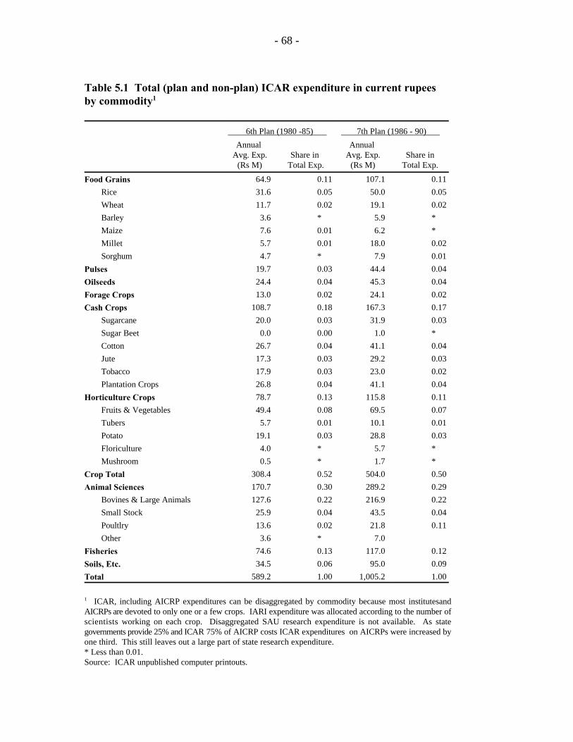
- 68 -
Table 5.1 Total (plan and non-plan) ICAR expenditure in current rupeesby commodity1
6th Plan (1980 -85) 7th Plan (1986 - 90)
Annual Annual Avg. Exp. Share in Avg. Exp. Share in (Rs M) Total Exp. (Rs M) Total Exp.
Food Grains 64.9 0.11 107.1 0.11
Rice 31.6 0.05 50.0 0.05
Wheat 11.7 0.02 19.1 0.02
Barley 3.6 * 5.9 *
Maize 7.6 0.01 6.2 *
Millet 5.7 0.01 18.0 0.02
Sorghum 4.7 * 7.9 0.01
Pulses 19.7 0.03 44.4 0.04
Oilseeds 24.4 0.04 45.3 0.04
Forage Crops 13.0 0.02 24.1 0.02
Cash Crops 108.7 0.18 167.3 0.17
Sugarcane 20.0 0.03 31.9 0.03
Sugar Beet 0.0 0.00 1.0 *
Cotton 26.7 0.04 41.1 0.04
Jute 17.3 0.03 29.2 0.03
Tobacco 17.9 0.03 23.0 0.02
Plantation Crops 26.8 0.04 41.1 0.04
Horticulture Crops 78.7 0.13 115.8 0.11
Fruits & Vegetables 49.4 0.08 69.5 0.07
Tubers 5.7 0.01 10.1 0.01
Potato 19.1 0.03 28.8 0.03
Floriculture 4.0 * 5.7 *
Mushroom 0.5 * 1.7 *
Crop Total 308.4 0.52 504.0 0.50
Animal Sciences 170.7 0.30 289.2 0.29
Bovines & Large Animals 127.6 0.22 216.9 0.22
Small Stock 25.9 0.04 43.5 0.04
Poultlry 13.6 0.02 21.8 0.11
Other 3.6 * 7.0
Fisheries 74.6 0.13 117.0 0.12
Soils, Etc. 34.5 0.06 95.0 0.09
Total 589.2 1.00 1,005.2 1.00
ICAR, including AICRP expenditures can be disaggregated by commodity because most institutesand1
AICRPs are devoted to only one or a few crops. IARI expenditure was allocated according to the number ofscientists working on each crop. Disaggregated SAU research expenditure is not available. As stategovernments provide 25% and ICAR 75% of AICRP costs ICAR expenditures on AICRPs were increased byone third. This still leaves out a large part of state research expenditure.* Less than 0.01.Source: ICAR unpublished computer printouts.
- 69 -
some oilseeds, public sector investments in research are matched by private sector
investments (Pray et al., 1991; Singh et al., 1995). Even within a commodity, there is no
evidence of systematic underinvestment in crop improvement research for rainfed areas, as
shown by the recent analysis of allocation of research resources to wheat improvement
research where rainfed areas receive a high share of resources relative to their contribution
to value of production (Jain, Byerlee and Traxler, 1996). In addition, the area of some rainfed
crops is declining over time due to low demand (e.g., sorghum and millet) or conversion of
land from rainfed to irrigated, requiring a decrease in the share of research resources invested
in these crops. Unfortunately there are no comparable data on the share of resources being
allocated to SWM research for rainfed areas. There are significant investments through
CRIDA and the all-India coordinated project for rainfed areas, but there is no baseline to
show to what extent there may be systematic under or over-investment in SWM research for
rainfed areas.
Approaches to Research
Tapping existing potential vs. developing new potential. Productivity increases can
be achieved both by encouraging farmers to attain yields that are achievable with existing
technology (closing the yield gap between research stations and farmers’ fields) and
developing new technologies that increase yield potential (widening the yield gap in the very
short term). These two approaches are not mutually exclusive, but rather can be carried out
side-by-side. Clearly, both approaches are important. On the whole, closing the yield gap
requires working relatively closely with farmers to identify the causes of their yield shortfalls,
while expanding the yield ceiling involves work mainly on research stations. Indian
agricultural research tends to focus heavily on on-station work compared to on-farm work,
suggesting that there are potential gains to be made from marginal increases in the allocation
of resources to on-farm work.
Shah and Sah (1993) present several types of evidence to support this contention.
Table 5.2 shows their assessment of differences between on-station and on-farm yields; they
point out that it is unlikely that this gap could ever be closed completely because farmers do
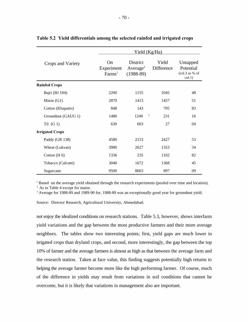
- 70 -
Table 5.2 Yield differentials among the selected rainfed and irrigated crops
Crops and Variety
Yield (Kg/Ha)
On District Yield Untapped Experiment Average Difference Potential
Farms (1988-89)1
2
(col.3 as % ofcol.1)
Rainfed Crops
Bajri (BJ 104) 2200 1155 1045 48
Maize (G1) 2870 1413 1457 51
Cotton (Khapatio) 848 143 705 83
Groundnut (GAUG 1) 1480 1249 231 163
Til (G 1) 630 603 27 04
Irrigated Crops
Paddy (GR 138) 4580 2153 2427 53
Wheat (Lokvan) 3980 2627 1353 34
Cotton (H 6) 1336 235 1102 82
Tobacco (Calcutti) 3040 1672 1368 45
Sugarcane 9500 8603 897 09
Based on the average yield obtained through the research experiments (pooled over time and location).1
As in Table 4 except for maize.2
Average for 1988-89 and 1989-90 for, 1988-89 was an exceptionally good year for groundnut yield.3
Source: Director Research, Agricultural University, Ahmedabad.
not enjoy the idealized conditions on research stations. Table 5.3, however, shows interfarm
yield variations and the gap between the most productive farmers and their more average
neighbors. The tables show two interesting points; first, yield gaps are much lower in
irrigated crops than dryland crops, and second, more interestingly, the gap between the top
10% of farmer and the average farmers is almost as high as that between the average farm and
the research station. Taken at face value, this finding suggests potentially high returns to
helping the average farmer become more like the high performing farmer. Of course, much
of the difference in yields may result from variations in soil conditions that cannot be
overcome, but it is likely that variations in management also are important.
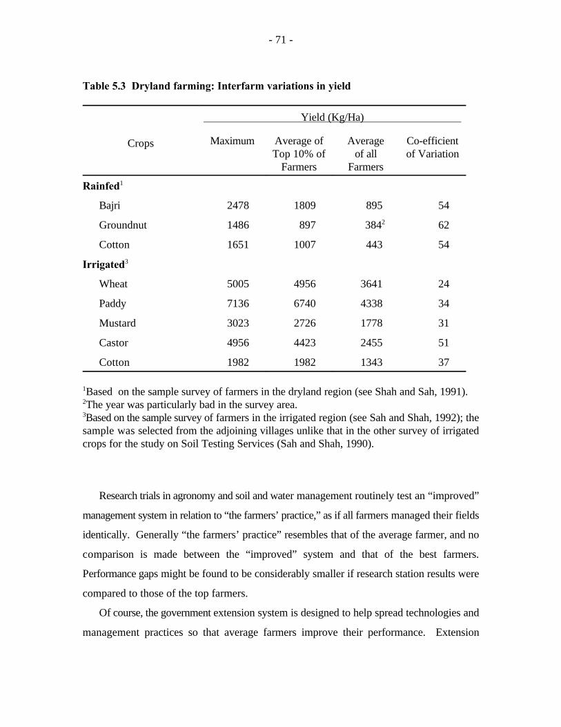
- 71 -
Table 5.3 Dryland farming: Interfarm variations in yield
Crops
Yield (Kg/Ha)
Maximum Average of Average Co-efficientTop 10% of of all of Variation
Farmers Farmers
Rainfed1
Bajri 2478 1809 895 54
Groundnut 1486 897 384 622
Cotton 1651 1007 443 54
Irrigated3
Wheat 5005 4956 3641 24
Paddy 7136 6740 4338 34
Mustard 3023 2726 1778 31
Castor 4956 4423 2455 51
Cotton 1982 1982 1343 37
Based on the sample survey of farmers in the dryland region (see Shah and Sah, 1991).1
The year was particularly bad in the survey area.2
Based on the sample survey of farmers in the irrigated region (see Sah and Shah, 1992); the3
sample was selected from the adjoining villages unlike that in the other survey of irrigatedcrops for the study on Soil Testing Services (Sah and Shah, 1990).
Research trials in agronomy and soil and water management routinely test an “improved”
management system in relation to “the farmers’ practice,” as if all farmers managed their fields
identically. Generally “the farmers’ practice” resembles that of the average farmer, and no
comparison is made between the “improved” system and that of the best farmers.
Performance gaps might be found to be considerably smaller if research station results were
compared to those of the top farmers.
Of course, the government extension system is designed to help spread technologies and
management practices so that average farmers improve their performance. Extension

- 72 -
services, however, operate on the principle of taking findings directly from the research
station to the farm. No emphasis is put on helping the average farmer learn lessons from the
best farmer. Some NGOs, notably the Aga Khan Rural Support Programme (AKRSP) in
Gujarat, have developed farmer-to-farmer extension programs designed explicitly to reduce
interfarm variations in performance by helping average farmers learn from better farmers.
One of the principles implicit in this approach is that even top-performing farmers operate
under conditions more similar to those of the average farmer than those of the research
station, so they may have more to offer to average farmers than would the extension worker
who brings knowledge from the research station. Impressive results have been achieved from
this approach; Shah and Kaul Shah (1994) report production increases of 30%-100% in the
project villages they study, though these gains result only partly from farmer-to-farmer
extension and partly from other sources. Farmer-to-farmer extension is also spreading in
other countries with growing success.
Need for farmer-based research. This review of the research directed to rainfed areas
indicates that much of the research has been experiment-station based using promising SWM
techniques as the point of departure for developing technological packages for rainfed areas.
In particular, there has been relatively little in depth research to understand traditional systems
and farmers’ rationale for following particular practices. Even the ICRISAT village studies,
while providing an excellent analysis of how factor markets work at the village level, devoted
relatively little attention to describing and understanding traditional farming systems. Where
in-depth efforts have been made to understand local systems, the results often suggest that
much of the technology being promoted to farmers is not relevant to their agroecological and
socioeconomic circumstances. Excellent examples include the careful studies of the
Bueshening system for rainfed rice (Fujisaka et al, 1991, Singh et al., 1994), which show that
practices used by farmers, such as high seed rates and ploughing of seedlings, provide similar
yield to recommended systems at lower costs and have other advantages such as more
dispersed seasonal labor use patterns, greater flexibility to withstand drought and floods, and
more yield stability. Similarly, Kerr and Sanghi (1992) describe farmers’ traditional SWM
practices and the rationale for their use. Once understood in terms of farmers’ objectives and

- 73 -
resources, the reasons for the low adoption rate of recommended SWM practices become
obvious. Likewise, detailed farm level studies in dryland Gujarat help identify the constraints
on soil fertility management under conditions of severe water stress (Shah and Sah 1993).
These examples indicate that the focus of research on SWM should now shift from the
research station to the farmers’ fields with farmers’ active participation. This implies the need
for detailed farm-level diagnostic studies to understand existing systems and practices in
different agroecological zones, combined with onfarm testing of promising technological
components identified in the diagnostic studies. It is also important that this work be closely
linked with work on the experiment station to ensure that findings from the onfarm work be
fed into the design of on-station research.
Such an approach to research is in its infancy in India, but it has shown that it can
yield valuable results. Pimbert (1991), for example, used matrix ranking and other
participatory rural appraisal (PRA) approaches to learn the preferences of groups of Indian
women farmers. Matrix ranking had the advantage of displaying the problem at hand in a way
that was easy for both farmers and researchers to understand. The women indicated
numerous uses of pigeonpeas, including grain to consume at home, grain to sell, leaves to
use as fodder, and stalks to use as construction material. They also listed various preferred
characteristics, such as seed yield, market price, pest resistance, storability, taste, and yield
and quality of leaves and stalks. Using matrix ranking, they indicated the relative importance
of each of these characteristics. They also explained that usually they plant more than one
variety in order to meet their various objectives.
Based on the information thus collected, Pimbert searched computerized databases
to identify varieties with characteristics likely to be attractive to the women farmers. He
found that some varieties that had been rejected by researchers had traits that were likely to
make them attractive to farmers. He then offered several varieties to the farmers, who
planted small amounts of each, including some local varieties, a variety that recently had been
officially released, and some improved varieties that had not been released. At the end of the
season, the women again used matrix ranking to rate the performance of each variety in terms
of all the criteria identified previously (figure 5.1). They found three unreleased varieties to

- 74 -
meet their various needs, but they unanimously rejected the officially released variety due to
its bitter taste.
Pimbert’s study shows the power of participatory research approaches to help guide
scientists to design technology that meets clients’ needs. In particular, he found that
scientists’ traditional focus on seed yield as the sole evaluation criterion led them to design
an unacceptable technology. Using information gained through participatory research,
subsequently they could reallocate their research resources more effectively.
Similar work is underway in collaboration between ICRISAT, ICAR and the
Government of Rajasthan to involve farmers in the selection of pearl millet varieties for
marginal environments. Sanghi (1989) reports initial efforts at participatory research in
dryland agriculture; Gupta (1991) and Sanghi et al (1994) present frameworks for organizing
and institutionalizing participatory work in the future.
Finally, it is important to point out that significant expansion of on-farm, participatory
research will require significant changes in the culture of agricultural research in India. To
date, on-farm research has been limited almost entirely to demonstration trials in which a
previous experiment is simply duplicated on a farmer’s field. Farmers have no little or no
input into these scientist-dominated exhibitions. Gupta (1989), arguing in favor of
participatory on-farm research, documents agricultural scientists’ attitudes that farmers’
indigenous practices are not worthy of study. Sanghi et al (1994) note that while farmers
rejected recommended soil and water conservation practices because they were not suitable
to existing farming systems, soil conservation officials and scientists believed the reason was
that farmers did not understand nor care about erosion. Such attitudes and approaches will
have to change if progress is to be made.
Package vs gradient approach to technology transfer. Closely related to the above
challenge is the fixation of the research system on developing technological packages for
rainfed areas. These packages have become steadily more complex over time as the strategy
has moved from SWM to include agronomic practices and various components of integrated
watershed programs. Yet packages are of dubious relevance in rainfed areas due to (1) the
diversity in time and space of production conditions, (2) risk factors (discussed below in

- 75 -
section 7), and (3) farmers’ resource constraints. The philosophy of most packages for rainfed
areas has been to replace traditional production systems with an entirely new system. An
alternative approach is to begin with farmers’ existing systems and introduce changes in a
stepwise manner from a menu of options from which the farmer can choose (Gupta, 1991;
Walker et al, 1982; Byerlee, 1994; Ryan and Subrahmanyan, 1975; Sanghi et al 1994). Such
a stepwise approach would allow technologies to be introduced that are consistent with
farmers’ objectives and resources.
Breeding strategies for rainfed environments. The above lessons also hold for
developing improved cultivars for and with farmers. A closer orientation to existing system
would enable the earlier identification of priority traits for different rainfed systems, such as
fodder yield and quality. In addition, there are two other unresolved challenges for breeders
targeting their products to rainfed areas.
The first of these is the relative emphasis to place on yield stability versus yield levels.
As discussed in more detail in section 8, some evidence suggests that yield variability of
HYVs is greater than for traditional varieties (Walker, 1989a). However, it is not clear if
improved yield stability would significantly improve adoption and farmers’ welfare, given that
yield variability is not a large component of income variability (Walker and Ryan, 1990). A
closely related issue is the emphasis on broad adaptation versus narrow specificity in variety
development. Since yield stability and adaptability are highly correlated (Binswanger and
Barah 1980), varieties that are stable over seasons are also likely to be fairly widely adapted.
However, some observers have argued for narrow specificity of adaptation of improved
cultivars and the involvement of farmers in improved cultivar selection (Maurya et al., 1988).
This issue may be more relevant for rice where micro level differences in rice ecologies due
to land type and water depth may be more pronounced than in dryland areas of Central and
southern India. Farmers often have identified particular local varieties for these different
ecologies and introduction of improved varieties will have to recognize these differences.
However, for dryland crops, inter-year differences may be more pronounced than inter-field
differences, suggesting the need for more widely adapted materials. In fact, the record of
- 76 -
adoption (see Section 3 above) supports the fact that widely adapted materials are also widely
adopted materials.
Research emphasis: breeding, crop management or SWM. A further unresolved issue
is the extent that research for rainfed areas should emphasize cultivar improvement, better
agronomic practices or soil and water management. The answer to this question is probably
quite location specific. In addition, there are significant complementarities between the three
technology groups. The above review has shown that improved cultivars have been widely
adopted in rainfed areas with a significant impact on productivity (although less than in
irrigated areas). Some agronomic practices have also been widely adopted, especially
fertilizer use. However, the role of research versus other factors such as extension, improved
infrastructure, and adoption of improved varieties in the spread of fertilizer use has not been
isolated. In general, research has played only a minor role in the first adoption of fertilizer
(Byerlee, 1994). Finally, adoption of SWM practices has been quite low, despite considerable
investment of research resources over the past two decades. Given that improved varieties
offer a proven track record of increasing productivity in many rainfed areas, there is a strong
case for maintaining continued strong crop breeding programs. However, to the extent that
the private sector is now able to meet the demand for improved varieties and hybrids for some
crops, there may be a case for consolidation of public sector programs.
While improved varieties can continue to be the lead technology in medium and higher
rainfed areas, the payoff to this effort will be higher with complementary investments in
improved agronomy and SWM practices. In addition, adoption of SWM practices may be
critical to preservation of the quality of the resource base (e.g., reduced soil erosion).
In the most marginal areas, improved varieties have generally had little impact and are
unlikely to have much impact without adoption of practices to improved moisture supply and
conservation. This implies that SWM will be the lead technology in these areas, although it
may be that there are many marginal areas where improved technology of any type will have
little impact. Thus the emphasis will differ by ecological region and over time in the same
region. However, to better inform decisions on resource allocation, there is an urgent need
to increase the capacity within the research system to measure and analyze the patterns of
- 77 -
research resource allocation between different types of research in different regions and to
analyze the impact of each type of research on productivity. Very little effort in the research
system is oriented to this type of analysis.
WATERSHED MANAGEMENT PROJECTS
As mentioned above, watershed management projects have become increasingly
widespread and increasingly complex in recent years. As they have come to represent the
principal vehicle for the transfer of rainfed agricultural technology, it is worth examining them
in detail to get an understanding of their performance to date and the issues they raise.
A watershed (or catchment) is a geographic area that drains to a common point, which
makes it an attractive planning unit for technical efforts to conserve soil and maximize the
utilization of surface and subsurface water for crop production. A watershed is also an area
that contains socioeconomic administrative and plot boundaries, lands that fall under different
property regimes, and farmers whose actions may affect each others' interests.
Socioeconomic boundaries, however, normally do not match biophysical ones. In watershed
management projects, mechanical or vegetative structures are installed across gullies and rills
and along contour lines, and areas are earmarked for particular land use based on their land
use classification. Cultivable areas are put under crops according to strict principles of
contour-based cultivation. Erosion-prone, less favorable lands are put under perennial
vegetation. This approach aims to optimize moisture retention and reduce soil erosion, thus
maximizing productivity and minimizing land degradation. Improved moisture management
increases the productivity of improved seeds and fertilizer, so conservation and productivity-
enhancing measures are complementary.
Excess surface runoff water is harvested in irrigation tanks while subsurface runoff
recharges groundwater aquifers, so conservation measures in the upper watershed have a
positive impact on productivity in the lower watershed. Reducing erosion in the upper
reaches of the watershed also helps to reduce sedimentation of irrigation tanks in the lower
reaches. The watershed approach enables planners to internalize such externalities and other
linkages among agricultural and related activities by accounting for all types of land uses in
- 78 -
all locations and seasons. This systems-based approach is what distinguishes watershed
management from earlier plot-based approaches to soil and water management.
The World Bank-funded Pilot Project for Watershed Development in Rainfed Areas,
which began in 1984, typifies the experience of the early, large scale integrated watershed
projects. Covering four watersheds averaging about 25,000 ha in four states -- Madhya
Pradesh, Maharashtra, Andhra Pradesh and Karnataka -- these projects pursued a highly
technocratic approach to soil and water management and afforestation. Trees, pasture
grasses and vegetative soil conservation barriers were planted, and farmers were told to
maintain them. Project managers soon realized, however, that unless inhabitants of
watersheds were convinced of the benefits of the new technologies introduced under the
project, they would not maintain them. The experience of this and similar watershed projects
gave rise to the new calls for people's participation.
"People's participation" gradually became a buzzword for watershed management and
other rural development projects in the late 1980s and early 1990s. While virtually everyone
agrees that it is a good idea, however, different people define participation in different ways.
Two extremes help to characterize the experience to date with participatory watershed
management. One extreme is based on the view that people will accept watershed technology
once they are made aware of its benefits; this requires a mechanism for project officials to
explain to watershed inhabitants what the work involves, how the various recommended
practices operate, and why it is important to adopt and maintain them. Taking people's
involvement a step further, in such projects local committees are established to mobilize
laborers for moving earth and planting vegetation, and to facilitate communication within the
village to improve the management of common lands.
The opposite extreme is based on the view that people know best how to take care
of their land and simply need outside assistance to help organize them and gain access to
resources, including funds and social services. Under this approach, project officials develop
mechanisms for local people to organize themselves, work collectively, and explain their
priorities for external assistance. Watershed projects that emerge from such a process tend

- 79 -
to pursue a combination of local soil and water management technologies with improved
agronomic practices.
While not necessarily reflecting these two broad extremes, most government projects
tend to operate closer to the first while many NGO projects resemble the second. Some of
the major issues confronting these projects are as follows:
Technical vs. Socioeconomic Orientation
As mentioned above, a watershed is both a technical and socioeconomic unit. While
both NGO and Government projects address both biophysical and socioeconomic
relationships in the watershed, government projects devote relatively more attention to
technical relationships while NGOs devote relatively more to socioeconomic relationships.
This can be seen in differences in the composition of project staff and the approaches to social
organization of watershed inhabitants, administrative organization, and technology choice.
Staff. Compared to NGOs, government project staff have more technical training but
less experience in working closely with community organizations.
Village-level institution building. NGOs approach watershed management as one of
a range of rural development activities that are chosen on the basis of villagers' priorities.
Since villagers rarely consider soil and water management to be their most pressing need,
watershed efforts often follow other types of projects that focus on income generation and
rural health, for example. Such projects tend to focus on building community-level
institutions that build organizational skills and support collective action. These institutions,
usually consisting of people of similar socioeconomic characteristics facing similar concerns,
become an asset once watershed management efforts are underway. Government projects,
on the other hand, also attempt to build local institutions to help implement watersheds and
build support among the people to maintain them over the years. In these projects, watershed
management (including treatment of private and common lands and support to livestock
owners) is introduced in isolation from other activities, and village-level organizations are
established solely to support the watershed project. Relatively less staff time is devoted to

- 80 -
support the local organization, and more is devoted to technical issues. This reflects the
composition of project staff mentioned above.
Administrative organization. Government projects are administered at the watershed
and microwatershed level, while NGO projects are more likely to be administered at the
village or miniwatershed level. (A microwatershed usually is larger than a village and may
contain parts of several villages, while a miniwatershed usually is smaller than a village and
usually is part of only one village.) Clearly there is a tradeoff between planning according to
the optimal biophysical unit (the watershed) as opposed to the optimal socioeconomic unit
(the village). Operating at the watershed level reflects the view that watershed management
is primarily a technological problem, whereas planning at the village level reflects the view
that watershed management is primarily a problem of social organization. It is important to
stress that planning at the watershed and village levels need not be mutually exclusive, since
watersheds consist of villages. With relatively small adjustments, government projects could
use the village as the planning unit and still adhere to watershed principles. Relatively minor
deviations from either the socioeconomic optimum or the technical optimum probably would
generate overall gains.
Technology choice. An analogous conflict takes place at the ground level in
implementing project works. Technologically optimal watershed management requires that
all bunds and ditches and cultivation adhere to contour lines. This approach, however,
conflicts with plot boundaries, which generally are aligned to slopes but not precise contours.
Contour-based watershed technologies interfere with farm boundaries and traditional
cultivation practices, imposing opportunity costs on farmers and slowing adoption.
Government projects adhere more strictly to contour based barriers and cultivation,
while NGO projects are more willing to accept barriers and cultivation across the slope,
aligned to plot boundaries. Also, government projects follow strict guidelines regarding the
dimensions and materials of bunds and other structures, whereas NGO projects are more
flexible, depending on farmers' preferences and locally available materials. Because watershed
management involves both physical and social processes, a compromise needs to be struck
that is both reasonably technically efficient and socially workable. More information is

- 81 -
needed on the tradeoffs involved in order to determine what is the most cost-effective
approach.
The Scale of Operations
Government and NGO projects tend to operate at very different scales. Government
projects cover vastly more territory, both relative to the size of the staff and in absolute terms.
This makes it difficult to compare the performance of NGO and government projects. Given
the small scale and higher intensity of human capital that characterize many NGO projects,
better performance than government projects is to be expected. This makes it difficult to
assess the effect on performance of differences in technology choice and social organization,
described above.
Another difficult question regarding the comparison between NGO and government
projects concerns the feasibility of "scaling up", or replicating the NGO approach to social
organization on a larger scale. The same degree of human capital intensity may not be
feasible in a large scale project, which in turn may constrain the degree of attention devoted
to social organization. This is a question that requires further consideration, and to which
several development agencies and researchers are devoting attention these days (e.g. the ODA
watershed project in Karnataka).
Employment Objectives vs. Watershed Objectives
All government watershed projects and most NGO projects double as employment
generation schemes. Government projects, for example, generally pay 90% of the cost of
works on private lands and 100% or works on common lands. Many NGO projects offer the
same subsidy as government projects, and practically all NGO projects offer a subsidy of at
least 50%. The majority of costs are for labor. Given that the minimum wage paid under the
project often exceeds the market agricultural wage, employment under the project is an
attractive activity for laborers and many farmers. As a result, in some cases employment
generation is the most important project component from villagers' perspective (Kerr and
Pender, 1996a). This creates the risk that villagers will accept project activities solely to gain

- 82 -
employment, with little interest in pursuing recommended practices or maintaining
engineering works or protecting permanent vegetation. There is ample evidence that this
problem occurs (Kerr, Sanghi and Sriramappa 1995).
While generating employment is a worthy objective that appeals to villagers, if it
interferes with watershed development objectives then perhaps the two should be separated.
If so, perhaps employment could be generated more cheaply and watershed management
could be promoted more effectively. This question needs examination.
Watershed Evaluations are Scarce
To date there are few comprehensive evaluation studies of integrated watershed
management projects. Some evaluations show considerable impacts on adoption of some
practices and on yields (see for example, the studies in the Indian Journal of Agricultural
Economics, Dec., 1991, referred to below in section 6). A few studies have computed ex post
cost-benefit ratios and shown a favorable ratio to the investments made. However,
inadequate data limits rigorous measurement of net benefits; there are few systematic
assessments of 1) the extent of adoption of watershed technologies and 2) their impact on
crop yields, runoff management and soil conservation.
Several reasons underlie the scarcity of information on project performance. First,
detailed farm-level data on crop yields and soil and water management are expensive and time
consuming to collect. Experimental data are available from watershed trials, mainly from
research stations. Some experimental data were collected on trials conducted on farmers'
fields but managed by project staff, so they do not reflect true farm-level conditions. Many
studies estimate net benefits of government or research station watershed projects by
calculating actual project costs, assuming yield impacts based on experimental data, and
assuming adoption and maintenance by farmers (e.g. Singh et al 1989). This approach is not
useful because too many assumptions are made in the absence of real data. On the whole,
watershed projects represent a lost opportunity to collect detailed data that would offer
clearer information about performance to date.
- 83 -
There is little evidence of sustained adoption of SWM technologies. Measuring initial
technology adoption is meaningless because it is so heavily subsidized. Only revisiting project
sites after the project has ended to assess the extent to which farmers continue to maintain
watershed practices would give accurate information about technology acceptance. Few if
any watershed projects commission evaluations of this nature. Some evidence suggests,
however, that even the subsidized engineering works have often been neglected on the
termination of the project (Kerr, Sanghi and Sriramappa, 1992).
Rigorous benefit-cost analysis is limited to a few highly successful, highly publicized
projects with a heavy infusion of technical assistance from state universities or ICAR
institutes, etc. (e.g., Singh et al, 1991; Dhyani et al, 1993). A few projects, such as
Sukhomajri in Haryana and Ralegaon Siddhi in Maharashtra, have received disproportionate
attention. These projects, however impressive, should not be taken too casually as replicable
models for other watershed projects. Both projects have certain unique characteristics not
necessarily replicable elsewhere, such as vast administrative support, favorable topographic
features, and single caste social structure in the case of Sukhomajri, and exceptionally
charismatic leadership in Ralegaon Siddhi. It is questionable whether these successes can be
replicated on a wide scale.
The few watershed evaluation studies that have been conducted raise a number of
issues with regard to design and implementation of IWM projects:
! What is the role of subsidies and credit versus farmers’ contribution of in kind
resources, especially labor, in adoption of SWM technologies?
! How can projects increase the participation of local people in the design and
management of the project?
! Can project complexity be reduced through focusing on a few components that are
most relevant in the local situation?.
! What institutional mechanisms can be used to design projects which are replicable
over a wider area and sustainable in the long term?

- 84 -
Repetto (1994, 26) points out shortcomings of the poverty line indicator and suggests7
that welfare improvements based on the poverty line are probably overstated. This is becausenoncash income sources, which tend to go unreported, are disappearing and being replacedby cash sources.
6. POVERTY AND RAINFED AGRICULTURE
Measuring poverty and relating it to the growth of rainfed agriculture is a complex
topic that we treat only briefly here. We refer to existing literature to review various aspects
of rural poverty, and we discuss poverty alleviation measures and their strengths and
weaknesses. The literature on poverty in India is large, so we cannot do justice to it.
Table 6.1 shows changes in the percentage of people falling below the poverty line in
different states between the years 1973-74 and 1987-88. Unfortunately this table does not
give us any indication of the distribution of poverty between rainfed and irrigated areas or
across different rainfed types, but it does show some important trends. In particular, the
percentage of rural people who are considered poor by the poverty line indicator has fallen
steadily in every state listed. This constitutes part of the evidence for what Singh (1990)7
refers to as the beginning of the “great ascent” out of poverty in rural South Asia.
Rainfed regions are characterized by higher poverty than irrigated regions. Table 6.2
shows clearly, for the year 1973, that the percentage of the population below the poverty line
falls steadily as irrigated area rises. The district database does not include information on the
number of people below the poverty line, so a rigorous analysis of the relationship between
irrigated area and percentage of people in poverty is not attempted here. State level data are
available, however, and can give us some indication. Table 6.3 shows the relationship
between the number of people below the poverty line and the percentage of rainfed area at
the state level for the years 1983 and 1987. The correlation coefficient is 0.45 for 1987,
suggesting a fairly strong relationship. The state level data, however, are too aggregated to
be very precise, and they do not distinguish between rural and urban poverty. Also, in this
approach tiny states like Tripura and Sikkim receive as much weight as large

- 85 -
Table 6.1 Changes in percentage of rural people falling below poverty line in majorstates, 1978-1988
StatePercentage of Rural People Falling Below Official Poverty Line
1977-78 1982-83 1987-88
Andhra Pradesh 48 38 27Bihar 63 63 64Gujarat 46 42 30Haryana 34 28 21Karnataka 55 48 36Kerala 59 52 39Madhya Pradesh 63 63 49Maharashtra 58 64 45Orissa 67 72 68Punjab 28 16 13Rajasthan 45 36 34Tamil Nadu 57 58 54Uttar Pradesh 57 48 46West Bengal 73 68 63
Source: Tables 4.2-4.5, Report of the Expert Group on Estimation of Proportion andNumber of Poor. Planning Commission, 1993.
Table 6.2 Percentage of population below the poverty line in relation to the percentageof area irrigated (1973)
Gross Irrigated Area as Number of Regions Percentage ofPercent of the Gross Cropped Population Below theArea in the Triennium Ending Poverty Line1973
Below 10 percent 16 68.75
10 - 20 percent 13 53.70
20 - 30 percent 10 45.62
35 -50 percent 8 48.39
Above 50 percent 7 26.46
Source: Rao et. al. (1988)

- 86 -
Table 6.3 Poverty and percentage of rainfed areas by state, 1983 and 1987
1983 1987
State Below Area Below Area% People % Rainfed % People % Rainfed
Poverty Line Poverty Line
Andhra Pradesh 29.88 63.40 27.20 62.70
Assam 40.86 84.60 36.84 84.30
Bihar 62.51 63.30 53.37 63.30
Gujarat 33.27 74.50 32.33 75.40
Haryana 21.24 36.40 16.63 30.90
Himachal Pradesh 16.39 82.90 15.46 82.90
Jammu & Kashmir 24.10 59.50 23.20 60.60
Karnataka 38.47 82.00 38.14 81.00
Kerala 40.91 85.30 32.08 85.20
Madya Pradesh 50.13 86.10 43.40 84.40
Maharashtra 43.54 86.90 40.10 87.60
Manipur 38.08 59.70 32.93 60.30
Meghalaya 39.46 76.40 34.60 75.20
Nagaland 39.75 71.70 34.85 71.20
Orissa 65.32 76.90 55.61 77.50
Punjab 16.29 9.50 12.70 8.70
Rajasthan 35.02 77.80 34.60 75.30
Sikkim 39.62 87.20 34.67 88.10
Tamil Nadu 52.38 50.50 45.13 56.30
Tripura 40.79 89.30 36.84 89.20
Uttar Pradesh 47.19 51.60 41.99 49.00
West Bengal 54.72 73.90 43.99 76.70
All India 44.76 69.30 39.34 68.60
Correlation coefficient 0.35 0.45
Source: Planning Commission 1993 and Area and Production of Principal Crops in India,various issues
- 87 -
states like Uttar Pradesh and Bihar. Therefore we should not draw strong conclusions from
this table.
As mentioned above, rural wages are an imperfect indicator of poverty. Repetto
(1994) examined changes in agricultural employment associated with growth in agricultural
output in the 1970s and 1980s. He found that on-farm employment actually fell in Haryana
and Punjab, where agricultural output grew the fastest. This information alone has little
implication for rural poverty, however, considering the fact that these two states have by far
the lowest levels of rural poverty in the country, in part because the green revolution also
stimulated strong growth in the nonfarm economy. Still, Repetto points out that over the
years, agricultural growth has had a less than commensurate effect on employment growth.
He cites Basu and Kashyap (1992) as finding that the employment elasticity of agricultural
growth declined continuously during the 1970s and 1980s. Each percent increase in
agricultural output yielded an increase in agricultural employment of 0.7% in the 1970s but
only 0.3% in the 1980s.
There has been a long debate about whether the productivity gains of the Green
Revolution resulted in welfare improvements for the rural poor. Ravallion and Datt (1994)
cited two studies, one that argued that “trickle down” of benefits to the poor has been a
reality, and another that argued that growth has led to increased inequality. These two studies
addressed roughly the same period of time, so their conflicting conclusions are surprising.
More recent empirical work has suggested that agricultural growth has in fact succeeded in
reducing poverty levels. Singh (1990) argued that all income groups gained from the green
revolution, but said it is “widely accepted” that wealthier groups benefitted more than less
wealthy groups. Hazell and Ramasamy (1991), on the other hand, show evidence that the
large income gains associated with the green revolution between 1973-74 and 1983-84 in
North Arcot, Tamil Nadu, did benefit landless and small farm households by at least the same
proportion as for large farm households. They found that a 4% decrease in total agricultural
employment was more than offset by large wage increases and increased off-farm employment
opportunities. Also, the lower on-farm employment figures reflected a drop in labor market
participation by members of households farming more than one hectare of land rather than the
- 88 -
landless or holders of even smaller plots. Larger farms also gained from the green revolution,
but less so due to larger cost increases they faced due to rising labor and fertilizer costs. The
conflicting findings of Singh, on the one hand, and Hazell and Ramasamy on the other may
reflect differences in the rate of adoption of green revolution technology. Hazell and
Ramasamy found that larger farmers adopted much more rapidly than small farmers, but after
ten years the use of green revolution technologies was scale neutral. They also showed that
smaller farmers were able to retain their land holdings despite their initially inferior position,
enabling them to remain in a position to make strong gains after they eventually adopted.
Also, Hazell and Ramasamy only studied one small region.
Hazell and Ramasamy also found that every additional rupee of value added in
agriculture stimulated growth in value added in the nonagricultural sector equivalent to Rs
0.80. This large multiplier effect has important implications for the role of agriculture in
stimulating widespread economic development. It also helps to offset concerns that may be
generated by the reports of the small impact of agricultural growth on agricultural
employment, cited above. Ravallion and Datt (1994), in a study of household data from 1951
to 1991, drew conclusions similar to those of Hazell and Ramasamy. They found that rural
economic growth spread gains evenly and so brought ample gains to the rural poor; rural
growth even helped reduce urban poverty to a certain extent.
A related debate addresses the question of whether urban or rural economic growth
has the greater impact on poverty alleviation. Ravallion and Datt (1994) found that urban
economic growth was associated with unequal distribution of benefits, so that its impact on
urban poverty alleviation was small and the impact on rural poverty was insignificant. This
contrasts sharply with their findings above regarding the favorable impact of rural economic
growth on poverty alleviation. Ravallion and Datt concluded that both continued rural
economic growth -- including growth in rainfed agriculture -- and a more equitable process
of urban growth will be important to poverty alleviation in the future.

- 89 -
SPECIAL PROGRAMS FOR POVERTY ALLEVIATION
The relatively favorable performance of better endowed rainfed regions was
documented in sections 3 and 4. Continued increases in productivity in such regions can be
expected to help reduce poverty, particularly in combination with efforts to improve
infrastructure and institutions critical for delivery of services. Likewise, widespread poverty
is likely to remain for a long time in poorly endowed areas less likely to enjoy high agricultural
growth and rising wages. For these areas even more than others, migration and development
of the nonagricultural sector must provide the solutions. Singh (1990), von Braun (1995) and
others, however, comment that while economic growth and diversification may be the
solution to long term poverty alleviation, the process takes too long to solve today’s poverty
problems. Growth on the scale required cannot happen overnight, and it takes time for it to
have a significant impact on poverty.
This is the rationale for the introduction of numerous special antipoverty programs
introduced in India beginning in the 1970s. The programs are intended to alleviate poverty
in the short term while seeking to stimulate economic growth that will reduce poverty in the
long term. Of the many central government schemes initiated in India, the largest are the
Integrated Rural Development Program (IRDP), introduced in 1978-79, and the National
Rural Employment Program (NREP), which began in 1980. The IRDP mainly provided
subsidies and credit to purchase livestock and milch animals, outlaying Rs 10 billion and
covering about 3 million families per year in the mid 1980s. This program, however, suffered
from difficulties in targeting benefits to the poor and encouraging repayment of loans.
Despite its large coverage, it paled in comparison with the needs of the estimated 260 million
rural people. The NREP focused mainly on employment, generating 350 million additional
days of employment per year through Food for Work programs that executed a wide variety
of public works projects, including roads, drinking water projects, small scale irrigation
works, soil and water conservation and afforestation (Dantwala, 1986, cited in Singh (1990).
Singh and Dantwala argue that employment programs have a greater capacity to help the
poorest people because they can be self-targeted, with less spillover than other measures such
as food aid, and they can also create durable infrastructure that leads to development.

- 90 -
Von Braun (1995) presents a conceptual model and detailed evidence of the positive
contribution that employment programs can make to poverty alleviation. He shows why
employment generation can be a superior alternative to other measures such as food subsidies,
which benefit poor people but are expensive, distort food prices, and suffer significant leakage
to nonpoor households due to targeting difficulties (Pinstrup-Anderson, 1988; Repetto, 1994;
Parthasarathy, 1995). Employment programs, on the other hand, can be self-targeted toward
poor people whose only productive asset is their labor. Employment programs can, in
principle, be self-financed though taxation that pays not only for employment but productive
assets and improved infrastructure that employment generates. In India, employment
programs have been used for constructing canal irrigation schemes, building roads and
drinking water wells and buildings. Eventually some concern arose that the opportunities for
productive, labor intensive infrastructure development were dwindling (Thomas Walker, pers
comm.). The amount of unutilized canal irrigation potential dwindled, virtually every village
had a school house and a health center, and road work was confined mainly to maintenance,
not construction of new roads. With the increased focus on developing rainfed agriculture
over the last decade, there has been an increased focus on using employment to support
rainfed agriculture. Watershed development, including soil conservation bunds and ditches,
check dams and tree planting, appeared to be a useful way to support the development of
rainfed agriculture in distressed areas while also providing short term employment
(Hanumantha Rao, 1992).
The focus on asset creation to support rainfed agriculture is attractive, but there is
insufficient information regarding its effectiveness to date. Jackson (1992), in a worldwide
study that included India, argued that the asset-creation impact of employment programs was
exaggerated due to the low quality of work they produce. Kerr et al (1994) argue that in
India, watershed development efforts linked to public employment programs are unlikely to
have a lasting impact on rainfed agriculture under current program design. They present
numerous field observations suggesting that soil and water conservation programs based on
employment programs may create illusory gains. This is because in order to obtain
employment at the minimum wage, which in some cases exceeds the market wage,

- 91 -
participants are encouraged to install mechanical structures that they may dismantle
immediately afterward, or to plant trees that they will not protect. For this reason, the link
between public employment and rainfed agricultural development may be more complex than
first thought. In fact, in several countries, particularly in Africa and the Caribbean,
employment subsidies have been separated from soil and water conservation programs
because the objectives of employment and natural resource management appeared to be in
conflict (Kerr et al, 1994).
The point is that long run asset-generation effects of employment programs should
not be taken for granted, particularly as related to rainfed agriculture. The papers in Von
Braun (1995), for example, examine in great detail the benefits of employment but largely
assume the durability of assets created. They devote more attention to whether such assets
will result in equitable income distribution than the amount of such assets they will actually
generate. Further research and field experimentation are needed to understand the nature of
incentives they create and the steps needed to ensure that they are consistent with long term
asset creation as well as short term poverty alleviation. Kerr et al (1994) suggest some ideas
tried on the ground in India and Africa to achieve that objective. Still, it may prove to be that
some kinds of assets, like roads, wells and buildings can be created more effectively through
employment programs than others, like trees and soil conservation bunds.
Other problems also remain with employment programs. Jackson (1992), for
example, argues that such programs often are associated with high leakage. Unpublished
ethnographic data from ICRISAT (1993, 1995) also cites villagers’ complaints of leakages
and favoritism in distributing employment benefits, but there is no evidence on the scale of
the problem. On the other hand, such government programs will always be associated with
some leakage, but that does not necessarily mean that they should be eliminated. In any case,
there is room for improvement in making employment programs more cost-effective.
Finally, one important aspect of employment generation programs is their capacity to
be self-targeting, with minimal distortion to the rural economy. These objectives can be
achieved if wages are kept slightly below the going market wage, and if they are concentrated
in the slack season, when employment demand is low. If wages are low, only those people
- 92 -
who really need them will participate. If they are high -- above the market wage, in particular
-- then employment will be rationed and some people who need it will not be able to get it.
Ravallion, Datt and Chaudhuri (1990), for example, found that raising wages may cause a
greater proportion of the poorest people who seek work to be excluded. This is so because
as program benefits become more attractive and have to be rationed, less powerful people will
have a more difficult time bidding for them.
Low wages also ensure that small farmers who rely on hired labor during peak periods
do not suffer from having to pay high wages due to labor scarcity created artificially through
public employment programs. Legislation in India requiring public employment programs to
pay the national minimum daily wage of Rs 22, though well-intentioned, may cause
employment programs to be less effective in reaching the poorest people, make them
financially unaffordable, and damage the interests of small farmers by raising wages above the
market wages that prevail in some areas.
GRASSROOTS ANTIPOVERTY INITIATIVES THAT SUPPORT RAINFEDAGRICULTURE
Over the years, Indian NGOs have experimented with a wide variety of grassroots
approaches to rural development. Some of these, honed by a relatively small number of high
quality NGOs, appear to have promise for poverty alleviation and increased productivity even
in marginal areas. The wide variety of approaches to community development defy easy
categorization, but to be brief, we outline a stylized example of the experience to date.
Many NGOs find that informal savings cooperative groups are high on the list of
villagers’ priorities for development assistance (Fernandez, 1991; G. Sriramappa, Oxfam, pers
comm.). Savings groups are established loosely, with members selecting the composition of
their own groups, and many groups, typically of homogeneous membership, often operate
simultaneously in the same village. Experience suggests that participation in these groups
helps people generate capital, develop organizational skills, build villagers' confidence to work
collectively, to seriously consider new investment opportunities, and to act where they never
bothered to previously (James Mascarenhas, OUTREACH, personal communication;

- 93 -
Parthasarathy, 1994). Active local groups can stimulate psychological incentives that
previously were stifled by cultural or political constraints.
Mascarenhas, et al (1991) and Fernandez (1993) discuss links between promotion of
such groups and the development of rainfed agriculture through watershed management.
First, participation in credit groups can help villagers save funds to invest in rainfed
agriculture. One common experience in MYRADA’s and Oxfam’s thrift group projects is
that even without any financial assistance, within a year or two participants find that their
greatest challenge is to figure out how to spend their savings. Second, developing and
strengthening cooperative groups prior to tackling watershed development helps villagers
build organizational and conflict resolution skills that are important in watershed management.
Third, the groups can serve as a focal point for spreading awareness about the benefits of
watershed development. In MYRADA watershed programs, existing cooperative groups
developed to solve an unrelated set of problems become a focal point for development of
rainfed agriculture.
Small group credit generation programs have multiplied rapidly in south India.
MYRADA’s and Oxfam’s thrift projects, for example, have tens of thousands of participants,
and they are spreading rapidly. Information about these projects is limited, and their potential
to promote rainfed agriculture through indirect means is not well understood. They are
worthy of further attention, both to understand the role they can play in alleviating poverty
and promoting rainfed agriculture, and to understand how to extend such an approach to a
state or national scale.
7. NATURAL RESOURCE DEGRADATION AND RAINFED AGRICULTURE
Natural resource degradation in rural areas is a controversial topic. There is a wide
range of opinions regarding its causes, extent, consequences, and even its definition.
Narrowly defined, degradation of a natural resource can refer to a permanent, irreversible loss
of its productive capacity relative to its natural state. In a broader, socioeconomic
perspective, on the other hand, often human use of natural resources may be taken for

- 94 -
granted, so the natural state is not particularly relevant. Productive capacity must be defined
in terms of a given use; exploitation of a natural resource may lead to a situation in which it
becomes unsuitable in one type of use yet still productive in another. Equally importantly, in
some cases losses in productive capacity at one point in time may be reversed later, because
human activity can also improve the productive capacity of natural resources. In discussing
degradation, therefore, it is important to be explicit about what we are talking about. We
follow Scherr et al (1995), who suggest that for policy purposes, a dynamic view of natural
resource degradation and improvement is most useful because it allows us to examine the
question of how human exploitation affects natural resource productivity under particular
uses.
There are many types of natural resource degradation, such as deforestation, soil
erosion and other types of soil degradation, loss or pollution of surface water or groundwater
supplies, and loss of resistance to pests and diseases. All of these have some relationship to
rainfed agriculture. Data on natural resource degradation are relatively sparse, and
information on the implications for productivity are still more rare. We draw on a small
amount of published data in this section to present some evidence about the extent and
implications of various forms of natural resource degradation. Then we discuss some
determinants of people’s actions that lead to degradation or improvement in natural resource
productivity.
SOIL DEGRADATION
Soil is the natural resource whose degradation causes the most widespread concern
about rainfed agriculture in India. Soil degradation comes in several forms, including erosion
by wind or water, and chemical deterioration such as loss of nutrients or salinization. Sehgal
and Abrol (1994) compile the available information on soil degradation and conclude that
erosion by water is the most widespread form of land degradation in India. Table 7.1 shows
ICAR’s official estimate of the distribution of lands affected by different types of

- 95 -
Table 7.1 ICAR’s estimate of area of land subjected to various forms of degradation (million hectares)
StatusLand subject to degradation Land subject to degradation
(including land slightly affected) (excluding land slightly affected)
Area Percent of total Area Percent of total
WaterErosion
148 45 122 37
WindErosion
14 4 13 4
ChemicalDeterioration
14 4 11 3
Water-logging
12 4 5 2
Not fit forAgriculture
18 6 18 6
Total AreaDegraded
187 57 169 46
UnaffectedArea
123 37 160 49
TotalArea
329 100 329 100
Source: Sehgal and Abrol, 1994.
Note: Numbers may not add up due to rounding errors.
degradation in the country. Water erosion is distributed throughout the country; its most
severe form is found in parts of Uttar Pradesh, Madhya Pradesh, Rajasthan and Gujarat that
are prone to wide, deep ravines that disfigure the land and make agriculture impossible. In
other areas, erosion gradually removes topsoil and reduces yields, but it does not cause much
land to be taken out of production in the short term. Wind erosion in India is confined to
desert regions of Rajasthan and Gujarat, but it is not a significant problem elsewhere. Salinity
is a serious problem affecting mainly irrigated areas; it causes severe productivity losses on
- 96 -
high potential lands; some lands are even taken out of production. Lands with other nutrient
losses are surprisingly small in area given the large area of drylands with soils that are
naturally deficient in nutrients and receive only small applications of fertilizer and organic
matter.
Sehgal and Abrol’s estimates of area under erosion exceed most of those estimated
elsewhere. Table 7.2 shows the figures derived from other studies. The various studies
address slightly different questions and use different methods to arrive at estimated figures,
so their comparability is limited. We use the Sehgal and Abrol study because it is based on
the most systematic assessment, following the guidelines in the Global Assessment of Soil
Degradation (GLASOD) (Oldeman, 1988). Sehgal and Abrol rely on several sources of
information, including a generalized soil map of India, remote sensing data from selected
areas, and published information on forestry and different soil degradation problems.
Estimated Rates of Soil Erosion and its Consequences
Estimates of rates of erosion and its consequences vary. Also, the impact on
productivity of a given rate of soil loss depends greatly on the soil type, its original depth, and
the time period over which the rate of erosion is sustained.
Aggregate figures on soil loss per hectare can be misleading, because often they are
estimated on the basis of soil loss measurements on individual experimental plots. Often
under this approach, all soil that erodes in a given area is assumed to disappear, to be lost
permanently. Observations on farmers’ fields in India, however, reveal that sometimes
erosion can be a loss to one farmer but a gain to another on whose land the eroded soil is
deposited. Many farmers actually encourage erosion on one part of a plot in order to
concentrate soil where it can contribute to greater overall productivity (Kerr and Sanghi,
1992). What this means is that a given estimated rate of soil loss for a given region probably
is accurate on some plots or parts of some plots, but other areas are probably losing a smaller
amount and some are probably even gaining more than they are losing.
With this caveat in mind, we present briefly some estimated rates of soil loss for India.
Singh et al (1992) produced an iso-erosion map of India that delineates areas by their rate of

- 97 -
soil loss per ha. On the high end, ravine areas (mentioned above) are estimated to lose over
40 tons/ha per year, and the Shivalik Hills at the foot of the Himalayas are thought to lose
over 80 tons/ha/yr. Rates in the Indo-Gangetic Plains are estimated at uniformly less
Table 7.2 Estimates of degraded area in India
Study Area CommentsDegraded
(million ha)
FAO/RAPA 172(1992)
Includes 127 m ha subject to erosion, 29 m ha fertilitydecline, 9 m ha waterlogging, 7 m ha salinizationalkalinization.
Dregne and 102Chou (1992)
This figure only refers to dry areas (but not deserts) totaling163 m ha according to the authors. Their figure includes 60m ha rainfed lands, 8 m ha irrigated lands, and 34 m harangelands. Forests are excluded. As a percentage of thearea studied, this estimate is relatively high.
Bentley 115(1984)
Bentley defined wastelands as land currently producing lessthan 20% of biological potential. His figure includes 15 mha of marginal agricultural lands and recently deforestedlands.
Bhumbla and 93Khare (1984)
If nonforest wastelands are included, this figure becomes129 m ha, the figure accepted by the National WastelandsDevelopment Board.
Gadgil et al 88(1982)
This estimate excludes cultivated lands. Degraded landsdistributed as follows: pasture lands 12 m ha, degradedforests 36 m ha, culturable waste 17 m ha, fallows 23 m ha.
Vohra (1985) 103 Distribution is as follows: 30 m ha forest land, 33 m hauncultivated land, and 40 m ha crop land.
World Bank 115-130(1988)
Includes 32-40 m ha of degraded land; the rest is similar toGadgil et al (1982).
Chambers, 109Saxena andShah (1989)
Refers to lands producing substantially below potential.Distribution is 38 m ha cultivated lands, 2 m ha strips andboundaries, 36 ma ha degraded forest land, and 33 m hauncultivated degraded lands.

- 98 -
than 10 tons/ha/yr, and those in peninsular India, excluding mountainous areas, range from
less than 5 to over 30 tons/ha/yr.
Dhruvanarayana and Ram Babu (1983) attempted to aggregate soil loss throughout
India. They estimated an average nationwide soil loss rate of about 16 tons/ha/yr, with about
29 percent of eroded soil being permanently lost to the sea. They also estimated that about
9 percent of the total soil lost nationwide was deposited into major reservoirs, reducing their
capacity by 1-2% annually. The remaining quantity of soil lost simply moved from one place
to another.
El-Swaify et al (1982) suggests that 11 tons/ha/year is an acceptable rate of erosion
on most soils because it is the rate of natural formation of new soil. Beyond 12 tons/ha,
erosion will cause soils to become continually shallower.
Unfortunately, the consequences of soil erosion are no better understood than the
rates. According to Dregne, quoted by Crosson (1994), there is an “abysmal lack of
knowledge“ about the productivity implications of soil erosion. Measuring erosion and its
productivity effects is expensive and time consuming, especially in semi-arid areas where
weather changes from year to year, so that data must be collected over several years in order
to understand biophysical relationships correctly. This situation has led to increased interest
in crop simulation models which, once they are validated under a wide range of conditions,
can provide information on erosion rates and productivity implications quite quickly.
Simulation models estimate the likely amount of runoff under different agroclimatic
conditions, such as rainfall, slope, length of slope, soil type and soil cover, and the likely
amount of erosion associated with that runoff under those conditions. The models
incorporate probable weather patterns based on decades of daily rainfall data. Then they use
crop growth models to estimate the impact on productivity. Littleboy et al (1996) used the
PERFECT model to relate yields to soil depth and simulated soil loss for given soil
conditions. They calibrated the model to conditions on red soils at ICRISAT, near
Hyderabad, and found relatively little short term yield decline, but a permanent, catastrophic
loss in yields after 40-90 years of soil erosion. The time horizon, of course, depends on
erosion rates associated with different soil management practices. Their findings showed that

- 99 -
alfisols with slope greater than 5% should not be cropped. Other simulation models of soil
loss have not been calibrated to agroclimatic conditions in India, but there is increasing
activity in this field, and new, more accurate information will probably be available in coming
years.
Sehgal and Abrol (1994) present estimates of the severity of erosion in India. They
cite experimental data on erosion-productivity relationships based on three-year experiments
on vertisols in Nagpur, Maharashtra, that shows very small losses if erosion is kept to less
than 10 tons/ha/year, but very high losses under higher rates of erosion. They find that
erosion at the rate of 10-20 tons/ha/year causes yields to fall by 7.8-34.3% per year, and
erosion at the rate of 20/40 tons/ha/year, causes losses of 58-68% per year. These findings
suggest that for most crops, erosion at rates of more than 10 tons per year would lead to
practically zero yield in less than two decades (table 7.3).
Such rapid losses in productivity are not without precedent. Alison (1973), for
example, says that millions of acres throughout the United States suffered such heavy rates
of erosion that cultivation became unprofitable until abundant use of fertilizer made it possible
to use them again. The restoration of such soils raises an important point regarding the
distinction between reversible and irreversible effects of erosion. Reduced soil depth is
obviously an irreversible effect of erosion, unless a plot actually receives soil deposits
resulting from erosion further up the slope. A sustained reduction in soil depth will eventually
make cultivation impossible, as mentioned above in the discussion of the findings of the
PERFECT model.
Other losses associated with erosion, on the other hand, are reversible albeit at a
potentially high cost. It is well-known that as soil erodes, disproportionately large amounts
of organic matter tend to be lost. According to Allison (1973), eroding soil can contain up
to five times as much organic matter as soil left behind. Experiments at ICRISAT found that
on plots that received applications of farm yard manure, it was found to be heavily
concentrated in eroded material (QDPI/ICRISAT, 1991, pg 6). Water holding capacity also
drops with erosion; this takes different forms in the short and long term. In the long term,
water holding capacity is permanently reduced because shallower soil contains less space

- 100 -
Table 7.3 Loss in crop productivity (yield) at different degrees of erosion, slope and soildepth
ClassRange
Loss in Productivity/Actual YieldQ/ha and (percent loss)
Sorghum Cotton Pigeonpea Groundnut Soybean
Soil Parameter: Erosion
e1: Slight 0.8 -- -- 1.0 --
(5-10t ha yr ) (2.5) (--) (--) (5.8) (--)-1 -1
e2: Moderate 5.9 1.4 4.1 5.9 6.0
(10-20t ha yr ) (18.5) (7.8) (21.5) (34.3) (29.8)-1 -1
e3: Strong 21.7 11.0 11.1 11.7 12.7
(20-40t ha yr ) (68.0) (61.1) (58.1) (68.0) (62.9)-1 -1
Soil Parameter: Depth
Deep -- -- -- 2.1 2.7
(>100 cm) (--) (--) (--) (12.2) (13.4)
Medium 14.1 8.4 5.0 0.6 3.0
(50-100 cm) (44.2) (46.6) (26.2) (3.5) (14.9)
Shallow 23.4 6.7 11.2 9.2 12.7
(<50 cm) (73.4) (37.2) (58.6) (53.5) (62.9)
Model Yield* 31.9 18.0 19.1 17.2 20.2
* Model yield with soil-site suitability at optimum (suitable) level

- 101 -
Farmers were asked to estimate changes in yield on a given plot over several years8
under two cases, one in which it is subject to erosion, and the other after conservationmeasures are adopted. They also indicated the amount of fertilizer and farm yard manure theyapplied to their fields and the amount of these inputs they expected would be lost to erosion.Regressions on the basis of these data yielded the perceived erosion-yield relationship, andalso the portion of yield resulting from loss of applied nutrients compared to other factors.Unfortunately, farmers were not asked to about the effect on yields of lost moisture lost due
to store water. In the short term, erosion is correlated with high runoff, indicating that when
erosion is taking place, the soil captures less moisture to supply to crops. When conservation
is introduced and erosion ends, however, moisture retention can be increased and organic
matter content can be restored.
This distinction between short- and long term impacts of erosion is important to
consider when trying to assess the aggregate impact of erosion on productivity. Sehgal and
Abrol (1994), for example, combine estimates of the extent of erosion in India with those of
its severity (table 7.4), and their findings are alarming indeed. They divide severity of
degradation into four categories: low, medium, high and very high. Low severity indicates
that yield losses resulting from degradation are less than 15%; medium means losses of 15%-
33%, high means that 33-67% of productivity is lost, so that cultivation is uneconomical and
other uses, like agroforestry, provide the only hope; finally, very high indicates that soil
degradation is so great as to make the soil unusable. Given these categories, it is difficult to
believe the finding that over 142 million ha suffer from “high” or “very high” severity of
degradation out of a total cultivated area of 187.7 million ha. This would imply that over
75% of the land cannot be cultivated economically, a conclusion not entirely consistent with
the observation that farmers continue to cultivate most of that land. Continued cultivation
is also inconsistent with the finding in table 7.3 that even moderate erosion would bring yields
down to practically zero in less than a decade on all plots subject to moderate erosion.
Experimental findings of high yield losses due to erosion are not greatly different from
rates estimated by farmers. Farmers interviewed in three villages in Maharashtra and Andhra
Pradesh estimated that yields would fall on eroding fields by an average of 5-10% per year,
depending on the village (Kerr and Pender 1996b). One of the villages, 8
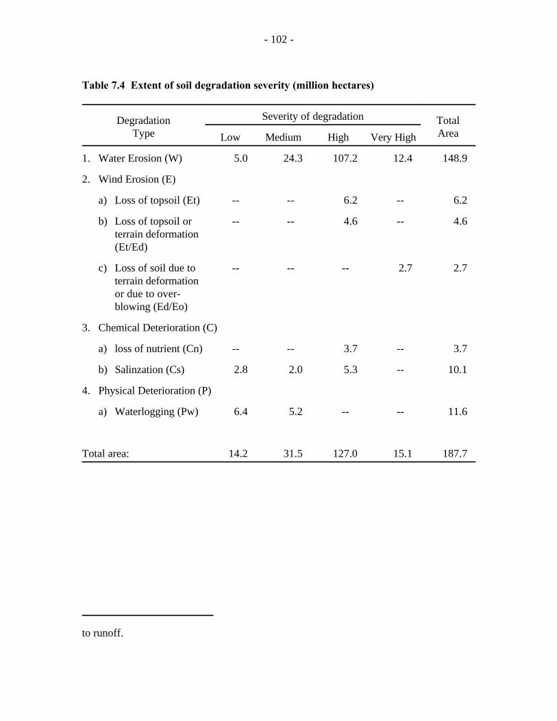
- 102 -
to runoff.
Table 7.4 Extent of soil degradation severity (million hectares)
Degradation TotalType Area
Severity of degradation
Low Medium High Very High
1. Water Erosion (W) 5.0 24.3 107.2 12.4 148.9
2. Wind Erosion (E)
a) Loss of topsoil (Et) -- -- 6.2 -- 6.2
b) Loss of topsoil or -- -- 4.6 -- 4.6terrain deformation(Et/Ed)
c) Loss of soil due to -- -- -- 2.7 2.7terrain deformationor due to over-blowing (Ed/Eo)
3. Chemical Deterioration (C)
a) loss of nutrient (Cn) -- -- 3.7 -- 3.7
b) Salinzation (Cs) 2.8 2.0 5.3 -- 10.1
4. Physical Deterioration (P)
a) Waterlogging (Pw) 6.4 5.2 -- -- 11.6
Total area: 14.2 31.5 127.0 15.1 187.7
- 103 -
Kanzara, has agroclimatic conditions similar to those in Nagpur, where the experimental data
reported in table 7.3 were generated. The farmers’ estimates are extremely rough, or course.
Nevertheless, the reported yield loss rates make an interesting comparison to the experimental
findings. Farmers’ yield loss rates appear to be on the low side compared to the experimental
data.
Farmers’ perceptions of erosion-yield relationships are consistent with the suggestion
that moisture retention and organic matter content can be restored after conservation
measures are introduced. Their responses suggest that farmers perceive that up to 25% of
the yield decline results from the runoff of farm yard manure and fertilizer they applied to their
fields. Farmers estimated that yields will rise by 3% to 14% per year when soil conservation
practices are put in place (Kerr and Pender, 1996b). Although these figures should be
considered as no more than rough indicators of farmers’ perceptions, it is clear that they do
not perceive productivity losses from erosion to be entirely irreversible. This makes sense in
light of the discussion above.
To summarize this section, evidence of declining yields associated with soil erosion
should be taken seriously, especially given predictions that irreversible losses due to reduced
soil depth will make cultivation impossible on many soils in less than a century. In addition,
experiments that show short term losses of 10%-50% resulting from erosion also imply a
serious reduction in current production levels. On the other hand, clearly there is a danger
in estimating all-India erosion rates by extrapolating from findings on small-plot experiments.
Likewise, it is important not to assume that evidence of short term yield decline represents
a permanent, monotonic relationship. More information is needed about spatial and temporal
variation in erosion rates under different biophysical conditions and management practices.
Costs and Benefits of Soil Conservation Investments
Data on the costs and benefits of soil conservation benefits are scarce. Some studies
have tried to estimate costs and benefits on the basis of experimental data of improved
practices. Even if their erosion-productivity data are accurate, their estimates of costs may
be inaccurate because, although they can capture cash costs of conservation investments, they

- 104 -
omit opportunity costs associated with changing other aspects of the farming system in order
to accommodate the improved conservation practice (Kerr and Sanghi, 1992). Other studies
use actual cash cost data from watershed projects and estimate the benefits on the basis of
either experimental data or observed field data for a year or two, and the assumption of
adoption and continued maintenance. These studies, however, are misleading because there
is little or no evidence of sustained adoption of recommended practices introduced under
watershed projects. In some cases farmers may selectively retain certain components of
watershed technologies (Joshi, 1995), but data are not available on the net returns to using
the components in isolation.
With this caveat in mind, we present some figures on the net benefits of improved soil
conservation from the Indian literature. The literature on costs and benefits of soil
conservation investments in India is large, even if most studies are not very comprehensive,
and we lack the resources to do justice to it here. A thorough literature review of watershed
and soil and water conservation literature from India will be conducted as part of the ICAR-
World Bank-IFPRI-ICRISAT rainfed agriculture study. The Indian Journal of
Agricultural Economics (1991) contains summaries of numerous evaluations of watershed
management projects. These projects include far more than just soil and water conservation;
for example, they introduce new seeds and other inputs, they try to increase grass and forest
cover and, in some cases, they even develop irrigation. In addition, the summary reports use
a wide variety of indicators of net project benefits, so direct comparison is not feasible.
Rather than recite the exact findings of the many studies listed in the volume, we simply list
a few general points.
! Many studies list cost-benefit ratios. In all cases they are greater than one, and in
some cases they range up to over 2.
! Two studies calculate internal rates of return. In one study the various project
components have rates of return ranging from 8-12%, including 10% for the soil
conservation component. In the other study the range is 12-15%, with 12% for the
soil conservation component.

- 105 -
! Many studies cite increased yields of various crops; they range from 10% to 100%.
Most of these studies do not provide information about net returns associated with
yield increases.
! Other studies cite qualitative improvements such as increased cropping intensity,
rising water tables, increased irrigated area, higher input use, and higher employment.
It is important to note that many of the studies compare performance in two years,
one before the project and another during the project. They attribute the improved
performance in the latter year to the watershed project. This method is flawed, however,
because any effect of a watershed project may be dwarfed by the effects of large swings in
weather. The studies that pursued this approach did not address this potential problem.
While many studies have evaluated the net benefits of watershed projects, they have
not followed a common methodology, and many of them present questionable results.
Clearly, further work is needed to take a more systematic approach to comparing watershed
management experiences under different circumstances.
Farmers’ Adoption of Soil Conservation Practices
Little work has been done on the determinants of farmers’ decisions regarding soil and
water conservation investment. Some studies address these questions in the context of special
soil conservation or watershed management projects but, as mentioned in section 4 the
relevance of this approach is questionable, because programs are so highly subsidized that
initial adoption is meaningless. A more useful approach would be to return to project sites
after they have been completed in order to assess farmers’ continued use of technologies and
practices introduced under a project.
Kerr and Sanghi (1992) and Pender and Kerr (1996) study the circumstances under
which farmers invest in soil conservation. These studies focus on areas that are outside of
watershed project areas, so farmers’ investments are unsubsidized. As a result, the
conservation practices in question are indigenous ones, not those introduced under watershed

- 106 -
projects. The differences in the two types of technology were discussed in the section on
agricultural technology.
Some of the findings of Kerr and Sanghi (1992) regarding technology design are
discussed above in section 5. They presented several hypotheses on the basis of field
observations and group interviews; we mention a few of them here. They suggested, for
example, that farmers invest in soil conservation at least as much for short term productivity
as long term conservation objectives, because soil conservation measures also conserve
moisture and organic matter. As a result, farmers are more likely to invest in conservation
on their most productive plots, even if they are not the most prone to long term erosion-
induced productivity losses. Kerr and Sanghi also hypothesized that farmers under tenancy
are unlikely to invest in soil conservation, because state laws in their study area (several south
Indian states) discourage tenancy, effectively limiting tenancy contracts to no more than two
seasons, and usually not more than one. As a result, tenants will not realize the long term
benefits of conservation investments. Another hypothesis is that farmers are less likely to
invest in soil conservation on dryland the more income they derive from alternative sources,
including irrigated land. The rationale for this hypothesis is that farmers with alternative
income sources will be less dependent on rainfed agriculture and thus less concerned about
its long term productivity. On the other hand, if credit markets are imperfect, farmers with
alternative sources of income might invest more because they are less constrained financially.
A related hypothesis is that farmers with more family labor available for agricultural work will
invest more in soil conservation, because the marginal product of their labor in other uses may
be lower. This argument is based on the view that in many cases soil conservation is an
activity with relatively low returns, so it is worth devoting a few hours of work here and
there, but not necessarily worth hiring workers for a full day at the market wage. This
argument would imply an imperfection in labor markets.
Pender and Kerr (1996) test these and other hypotheses about soil and water
conservation investments in the same study area. Their preliminary econometric findings
support the hypotheses that plots under tenancy receive less investment than owner-operated
plots, and that farmers tend to invest in their best plots first. They found mixed evidence
- 107 -
about the effects of family labor and alternate income sources, depending on the village.
These differences can be explained in part by the diverse agroclimatic conditions across
villages, which may change the benefits of soil and water conservation investments. This
research is still in progress, and alternate specifications of the model may yield additional
information or clarify some of the ambiguities in the preliminary results.
Waterlogging, Salinization and Alkalinization of Irrigated Lands
This is potentially a very serious problem for Indian agriculture because it affects the
most fertile lands in the breadbasket areas of Punjab, Haryana, and northwestern Uttar
Pradesh. Estimates of salt-affected lands also vary greatly, ranging from about 3 million ha
(Joshi and Singh 1991) to about 25 million ha (Bowonder and Ravi 1984). Joshi and Jha
(1991) found that after 10 years of salt accumulation, rice yields declined by 61% and wheat
yields by 68%. Some soils in rainfed areas also suffer from salinization, but the area affected
is smaller and the absolute yield decline is smaller. But salinity and alkalinity on irrigated
lands affect rainfed agriculture indirectly, because it increases the need for production on
rainfed lands to augment production on irrigated lands.
In many places salt-affected lands are taken out of production completely, but this
need not be the case. The Central Soil Salinity Research Institute has developed salt-tolerant
HYVs of rice and wheat, for example. Also, large amendments of gypsum and other
chemicals and minerals can remove salinity, though eventually it may return. In the longer
term, better drainage is needed in order to reduce the water table in irrigated areas. In many
cases this requires significant up-front investment, and also collective action among area
farmers to ensure that drainage is managed properly across several farms.
Joshi (1996) discussed the conditions under which farmers will invest in soil
amendments to neutralize soil salinity by comparing the cases of Punjab, Haryana and Uttar
Pradesh. He found that the extent of investment depends greatly on the alternative options
for investment open to farmers. In Uttar Pradesh, many plots remain fallow and there remains
significant unexploited groundwater irrigation potential. Farmers with saline lands often find
it more profitable to sink a well on a neighboring plot, for example, or to increase fertilizer

- 108 -
applications on another plot, than to invest in reclaiming a salt-affected plot. In Punjab and
Haryana, on the other hand, groundwater potential is almost completely exploited, and there
are relatively few other investment opportunities to increase land productivity. As a result,
investment in reclamation of salt-affected soils is quite high. Joshi estimates that 42% of salt-
affected plots have been reclaimed in Punjab and 36% in Haryana, but only 11% in Uttar
Pradesh.
Joshi recommended that credit programs are needed to encourage private land
reclamation. Drainage, meanwhile, requires government assistance because it must be
addressed on a scale larger than an individual farm or even a village. Efforts are needed to
encourage farmers to act collectively to maintain drainage arrangements.
Groundwater Degradation
Groundwater is another resource that, in many places, is inextricably linked to rainfed
agriculture. This is especially so in semi-arid areas with unreliable monsoon rains. Although
access to groundwater immediately converts a rainfed agricultural plot to an irrigated plot,
it still has important implications for dryland farming because virtually all farmers with wells
also operate rainfed plots, and they allocate their time and financial resources between
irrigated and rainfed agriculture. Likewise, through joint ownership of wells and groundwater
market, the percentage of farmers with access to some irrigation greatly exceeds the
percentage of area irrigated (Mehra, 1995; Shah, 1993). Walker and Ryan (1990), in fact,
cite farmers’ interest in irrigation as a major constraint to adoption of improved dryland
agricultural practices: farmers would rather allocate their money to irrigation wells than
dryland technologies. Although wells have only moderately high expected rates of return
(Pender, 1993), farmers prefer to invest in them in part because of the relatively stable
production obtained through irrigation.
Groundwater is a difficult resource to manage, especially in hard rock areas
characterized by low groundwater recharge and small aquifers whose boundaries are not
known. Irrigation wells have existed for centuries in India, but they have only become
widespread in the last couple of decades, as a result of easy access to electricity and diesel
- 109 -
fuel. In some areas, groundwater exploitation has reached such an advanced stage that water
tables are falling in some places by more than a meter per year, so that farmers have to deepen
their wells every few years to retain access to water (Vaidyanathan, 1994, cited by Repetto,
1994). In some areas, deep drilling has led to saltwater intrusion into aquifers, rendering
water unfit for agricultural or domestic use.
Two factors have contributed to growing scarcity of groundwater in many areas in the
last decade: low, flat rate prices for electricity to power wells, and the absence of property
rights to groundwater. Regarding property rights, anyone in India who owns a plot of land
has the right to sink a well and extract virtually as much water as they please. Aquifers,
however, underlie a great many plots, so one person’s pumping may reduce another’s access
to groundwater. Wealthier farmers have a competitive advantage over their less wealthy
counterparts in this process, because wealthier farmers can more easily make the repeated
investments to deepen a well. State governments have introduced some restrictions intended
to prevent the digging of new wells in areas with too much pressure on groundwater, but as
Repetto (1994) points out, such provisions only solidify the gains that wealthier farmers made
by investing in wells first. Less wealthy, later adopters are unfairly excluded. This inequality
is reinforced by subsidies for credit, fertilizers and other inputs that are used more intensively
by farmers with irrigation (Repetto, 1994).
Shah (1993) suggests mechanisms to convert groundwater from an open access
resource to a community-based common property resource with well-defined rights for local
users, but numerous logistical difficulties pose a serious challenge to such efforts. Despite
the difficulties, ultimately such an approach is probably the best hope for a property rights
specification that generates an allocation pattern that is efficient, equitable and
environmentally sustainable.
Most states have charged flat rates for power consumption since the early 1980. Flat
rates are easier to administer than per unit pricing, but they have serious, negative implications
for groundwater management in water-scarce areas. Under flat rate power tariffs, there is no
relationship between the quantity pumped and the tariff paid, so well owners have an incentive
to pump water until the average product is practically zero. Farmers have responded
- 110 -
Panchayats could play a role in groundwater management if they are strengthened.9
Panchayats are discussed further in section 7.
predictably, planting water-intensive crops such as sugarcane and paddy. State electricity
boards have resorted to quantitative rationing to limit pumping, and higher tariffs to industrial
users that effectively subsidize agricultural use. The results are scheduled and unscheduled
power cuts for industrial, agricultural and residential users; structural imbalances in the
allocation of power between sectors; and continuing deficits for most state electricity boards
(Kerr et al 1996).
Some analysts have suggested that higher flat rate tariffs will solve the problems facing
electricity boards. Kerr et al (1996), however, demonstrate that even high flat rates do not
create an incentive for farmers to reduce pumping, because once the fee is paid there is still
no relationship between the amounts pumped and paid. The high fixed fee may also be
inequitable, because it may constrain cash-constrained farmers from purchasing an electricity
connection in the first place.
Property rights and power tariff problems may have to be solved jointly, through
collective property rights to groundwater. As mentioned above, Shah (1993) suggests some
cooperative approaches to groundwater management. Kerr et al (1996) suggest that property
rights and power tariffs could be village-based, with laws to designate the relative rights and
duties of farmers who own wells and those who don’t. This would be a second-best solution
that ignores the fact that aquifer boundaries and village boundaries do not match, but it may
prove to be a pragmatic compromise given the difficulty of mapping aquifers and organizing
people around aquifer boundaries.9
So far we have focused on the problem of groundwater scarcity in relatively dry areas.
In many canal command areas, on the other hand, environmental problems associated with
groundwater paradoxically result from its underexploitation. This is because in canal
command areas, pumping groundwater has the beneficial effect of reducing the threat of
waterlogging and salinization by lowering the water table, which tends to be high in surface
irrigated areas. Farmers in such areas have less incentive to develop groundwater resources

- 111 -
because they already enjoy virtually free access to surface water. In these areas, exploiting
groundwater is associated with positive externalities and thus should be subsidized by the
government. Low, flat rate prices make sense under these circumstances (Shah 1993).
Finally, Repetto (1994) points out that groundwater remains underexploited in higher
rainfall areas of eastern India. This is attributed to the lower marginal benefits of irrigation
in such areas than in semi-arid regions; the poor state of rural electrification and other
infrastructure that is conducive to agricultural intensification; and complex tenure
relationships that inhibit expensive, long term land improvement investments.
Degradation of Uncultivated Lands
The poor condition of India’s village forest and pasture lands evoke stark images of
the “tragedy of the commons.” Jodha (1992) documents the breakdown of traditional
mechanisms to govern use of common lands and the severe consequences in terms of decline
in their area, productivity and employment generation. Area under common lands declined
by 30-50 percent in 8 semi-arid states between 1950 and 1980. Bentley (1984) estimates that
over 80% of India’s 123 million hectares of uncultivated lands produce 20% or less of their
biological potential. He argues that low productivity is particularly acute on the common
lands that make up most of this area.
While about 23% of India’s territory is officially classified as forested, the area
actually covered by trees is no more than about 10-12% (Bentley, 1984; CSE 1982). Some
forest lands have been converted to grazing pasture, but these too are unproductive (Gadgil,
1982). The resulting shortage of biomass has significant implications for the development of
rainfed areas. One well-known problem is that villagers have to look for other fuel sources
in addition to wood to cook meals and heat water. Chambers et al (1989) cite UNDP figures
showing that the real price of firewood in rural areas doubled between 1973 and 1975.
As a result, cow dung has a high opportunity cost for use as fuel, so its application to
crops has declined (Motavalli and Anders 1991). Farmers correctly perceive that manure has
residual productivity effects lasting up to three years, but many farmers do not apply manure
so frequently. In dryland areas, irrigated plots and the most productive dry plots receive

- 112 -
manure more manure than less productive dry plots. Motavalli and Anders found that about
70% of irrigated plots received manure at least once every three years; the figure for dryland
plots was less than 20%. Biomass shortages also limit farmers’ ability to retain stubble on
crop lands during the dry season. Farmers cut as much stubble as possible to use as feed or
fuel, and grazing animals finish what is left. The bare soil that remains is highly prone to
erosion by early rains. Cogle and Rao (1993) report that applying straw mulch to alfisols
greatly raises yields by increasing infiltration and reducing erosion, and that this practice
would pay for itself within a few years. It is not known if farmers will be willing to adopt this
practice, however, given the high, immediate demand for fodder and the scarcity of capital
with which to make long term investments.
The decline in forest cover has other negative implications for rural areas. Gupta
(1982) estimated that for every person directly employed in forestry, four are employed
indirectly though forward linkages. Gupta (1982) also estimated that nontimber forest
products generated 2 million man-years of employment in India, and that the number could
be more than doubled if markets were better developed. Bentley (1984) pointed out that a
much larger increase could be realized if uncultivated lands were managed for higher
productivity. Jodha’s (1990) finding that common lands in 24 villages in 8 semi-arid states
generated an average of about 150 employment days for poor families further demonstrates
their employment potential. In these same villages, the poorest families derived as much as
25 percent of their incomes from common lands.
Numerous causes underlie the decline in production of common lands; we mention
them only briefly here. Repetto (1994) (citing Jodha 1992 and Agarwal 1992) outline some
of the traditional mechanisms for managing village common lands in pre-colonial times and
their emphasis on sustainability. The British Colonial administration usurped the ownership
of these lands, managing them as a source of government revenue and natural resources to
support the colonial economy (Bentley 1984, Gadgil and Guha, 1992). An adversarial
relationship between villagers and Forest Departments developed as early as the late 19th
century, when villagers were deprived of their traditional rights to natural resources that were
an integral part of their local economy (Gadgil and Guha, 1992). Independence did not
- 113 -
change this situation as the new government retained the same approach to forest
management. Government policies also reserved many areas for forest-based industries,
which received access to forest products at heavily subsidized rates and with little or no
obligation to manage forest resources on a sustainable basis. People living in forest areas had
little stake in the long term health of forest resources because they would be excluded from
the benefits. As a result, they would intrude on the forests when they could, illegally taking
what resources they could.
On common lands not managed by Forest Departments, the colonial administration
nurtured relationships with large landlords (zamindars) who took responsibility for enforcing
restrictions on the use of common lands. The zamindari system worked from the perspective
of managing natural resources, but it was feudalistic in nature, with highly inequitable
distribution of benefits. After Independence, the new government stripped zamindars of their
power and with it, the effective systems for restricting the exploitation of common lands.
State governments attempted to take responsibility to manage common lands but with poor
results (Bentley 1984).
Responses to the Declining Productivity of Common Lands
Declining productivity of common lands has stimulated two kinds of responses. One
response is action by government and nongovernment organizations to develop special
programs to manage forests and pastures, and the other is a spontaneous response by rural
people to either manage these lands differently or develop new ways to produce the goods
that the commons no longer supply. We discuss each of these in turn.
Government initiatives. Special programs come in many forms. Among the largest
has been the government’s effort to promote social forestry, in which the state Forest
Departments involve rural people to manage trees, rather managing trees to the exclusion of
rural people. Table 7.5 shows that between the 1950s and 1980s, the government both
greatly increased its emphasis on tree production and changed its approach to doing so.
Under social forestry, the aim was to grow trees on village common lands, roadsides, and
private plots, rather than in the reserved forests where people were not allowed.

- 114 -
Table 7.5 Forestry expenditures in the 1st and 6th plans
Social Forestry Reserved Forests
ha (mill) percent ha (mill) percent
1st Plan 15 29 37 71(1951-56)
6th Plan 1524 71 624 29(1980-85)
Source: Bentley, 1984
In the initial efforts to promote social forestry, production was concentrated on
private lands, while common lands remained unproductive, with low survival rates (Bentley
1984). Social forestry projects often worked with private farmers simply because it was
easier to grow trees on private than common land. There was nothing particularly “social”
about such forestry initiatives. Following this experience, more recent projects working on
common lands have tried to organize and motivate people to act collectively to protect trees.
These projects have had mixed success, in part because of differences in the way they are
managed (Hinchcliffe et al, 1995; Kerr and Pender, 1996a, but also because of differences in
communities: some communities may be more willing to engage in collective action than
others (Wade, 1988).
Legal rights of villagers may be critical to the success of efforts to develop common
lands. There is growing appreciation of the fact that under Indian forest laws, local people
have had very limited rights to the products of forest lands, and this has reduced their
incentive to protect them. This realization led to the development of Joint Forest
Management, an arrangement that represents a compromise between state ownership of forest
lands and increased access rights for local people. Under Joint Forest Management, villagers
receive a certain percentage of the proceeds of timber sales; they also own the rights to all
nontimber forest products. The logic is simple: villagers will have more incentive to protect

- 115 -
the forest if they own a share of the benefits. Institutions for collective action within villages
still need to be strengthened, but Joint Forest Management is a step that will increase the
returns to collective action. Joint Forest Management is a recent initiative; it will take more
time to judge its performance.
The new Panchayat Raj law is a more broad-based initiative to transfer rights and
responsibilities for various aspects of the rural economy, including natural resource
management. Although this movement is in its infancy, in some respects it represents a return
to precolonial systems of village level autonomy. Villagers will determine how and where to
invest public funds for development of their economy, and they will make and enforce rules
for managing many natural resources. This will provide an interesting test of the hypothesis
that villagers manage common property natural resources poorly because they are alienated
by laws that limit the benefits they can obtain from them. The Panchayat Raj is discussed
further in section 9.
Rural people’s actions. As mentioned above, rural people have also acted
spontaneously to cope with the reduced area and productivity of common lands. These
spontaneous actions receive less attention than special government and NGO projects, but
they may be more significant because they represent endogenous change with concrete
results. Farmers have shifted their cropping patterns in response to the decline of government
and common lands. Trees, for example, are increasingly cultivated by private farmers for sale
to industrial users in large cities. Table 7.6 shows how timber prices rose between 1970 and
1987 relative to other prices; it is easy to see why farmers responded to these prices by
growing timber. Eucalyptus plantations surrounding Bangalore, for example, bear testimony
to this change in the sources of timber. Private tree cultivation has generated so much supply
in north India that markets crashed, leaving tree growers with large losses (Saxena 1990).
Farmers’ choice of sorghum varieties is a case in which farmers have changed their
cropping patterns at least partly in response to declining fodder production on common lands.
Kelley et al (1993) document farmers’ shift toward sorghum varieties that produce more
straw, relating it to an increase in the price of fodder relative to the price of food grain. In
this way, crop lands substitute for common lands to produce fodder.
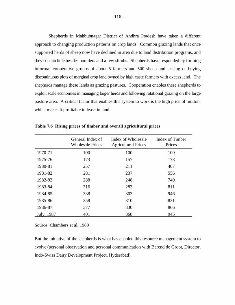
- 116 -
Shepherds in Mahbubnagar District of Andhra Pradesh have taken a different
approach to changing production patterns on crop lands. Common grazing lands that once
supported herds of sheep now have declined in area due to land distribution programs, and
they contain little besides boulders and a few shrubs. Shepherds have responded by forming
informal cooperative groups of about 5 farmers and 500 sheep and leasing or buying
discontinuous plots of marginal crop land owned by high caste farmers with excess land. The
shepherds manage these lands as grazing pastures. Cooperation enables these shepherds to
exploit scale economies in managing larger herds and following rotational grazing on the large
pasture area. A critical factor that enables this system to work is the high price of mutton,
which makes it profitable to lease in land.
Table 7.6 Rising prices of timber and overall agricultural prices
General Index of Index of Wholesale Index of TimberWholesale Prices Agricultural Prices Prices
1970-71 100 100 100
1975-76 173 157 178
1980-81 257 211 407
1981-82 281 237 556
1982-83 288 248 740
1983-84 316 283 811
1984-85 338 303 946
1985-86 358 310 821
1986-87 377 330 866
July, 1987 401 368 945
Source: Chambers et al, 1989
But the initiative of the shepherds is what has enabled this resource management system to
evolve (personal observation and personal communication with Berend de Groot, Director,
Indo-Swiss Dairy Development Project, Hyderabad).

- 117 -
In addition to shifting cropping patterns, villagers in many places have changed the
way they manage common lands. Privatization of the commons has occurred in many places.
In most areas the privatization process reflects the problem more than a response to problems
of common land management, as populist government programs distribute ever more marginal
lands to landless constituents (Pender and Kerr, 1996). In some areas, however, villagers
have taken the initiative to privatize common pasture lands informally. Kerr and Pender
(1996a) document this process for the case of grazing pastures in southeastern Rajasthan;
they find that both visual evidence and most biological indicators suggest private pastures are
better managed than their common counterparts.
In other cases, the outcome of greener pastures or more productive forests may be
attained through alternate approaches. Anecdotal information abounds of cases of successful
collective action to manage village common lands productively. Honey Bee (1995), for
example, cites the case of Mr. Balvantsinh in the village of Takhua, Banaskantha district,
Gujarat who, alarmed by the degradation of common lands in his village, single-handedly
mobilized his fellow villagers to protect common lands. In this particular case, linking the
management of the commons to religious practices and associated duties was a critical
element in making the management system work. Though cases such as this one appear to
more of an exception than a rule under current conditions, they do provide evidence that
collective action can work. More significantly, they demonstrate the capacity of local
institutional innovation to develop a system that is appropriate to the prevailing
circumstances. Legal reforms that guarantee villagers greater benefits from protecting the
commons will support such efforts. The Panchayat Raj and Joint Forest Management are
prime examples.
These examples of spontaneous responses to the problems of declining productivity
of common land resources demonstrate the need for caution when documenting resource
degradation and estimating its impact on the rural economy. These few examples, some
isolated and others widespread, probably have innumerable counterparts that can be observed
easily if the effort is made to search for them. Declining productivity of the commons does
not occur in isolation; rather, rural people devise mechanisms to cope with the consequences
- 118 -
The coefficient of variation is equal to the standard deviation divided by the mean.10
of reduced productivity of common lands. Simple indicators of the consequences of the
declining commons may be misleading as a result. This is not to suggest that some people are
not hurt by the declining productivity of the commons; Jodha (1990), for example, shows that
the poorest people suffered the most from the declining commons. But there is a need to take
the next step of finding out how such people have responded to changing circumstances. If
the rural economy has changed significantly, they may have replaced their dependence on the
commons with some other livelihood strategy. The low-caste shepherds of Mahbubnagar,
mentioned above, initially suffered from the decline of common grazing pastures, but now
they are among the wealthier groups of villagers (personal communication, Y. Mohan Rao,
Senior Research Associate, ICRISAT).
8. RISK AND RAINFED AGRICULTURE
Rainfed agriculture in semi-arid or sub-humid regions is generally risky and unstable.
Rainfall in the semi-arid tropics is not only low, but also unreliable, with a higher CV than in
more humid areas. Weather-related risk places hardship on people in these areas, and it may
constrain adoption of more productive agricultural technology. In this section we review the
evidence on instability and its consequences, and we discuss some mechanisms to alleviate the
problems.
INSTABILITY OF RAINFED VS. IRRIGATED AGRICULTURE
Agricultural yields are more unstable in rainfed areas than where irrigation is assured.
But if irrigation water supplies fail, then irrigated agricultural area can fall sharply, leading to
even more unstable output than under rainfed agriculture.
Dhawan (1988a) used the coefficient of variation (CV) as the indicator of instability10
of production, yield and area cultivated for irrigated and rainfed food grains. Using national
data, Dhawan found that the CV of output of unirrigated food grains for the period 1970-83

- 119 -
was 11.4%, significantly higher then the 6.4% for irrigated food grains. Decomposing these
into output and yield instability, the CVs of yield were 9.2% and 5.3% for rainfed and
irrigated food grains, respectively, and for area they were 3.1% and 2.3%, respectively. This
suggests that yield and area moved together to increase output instability.
Shah and Sah (1993) also found higher yield variations in rainfed than irrigated crops.
They calculated CVs ranging from 36% to 70% for yields of rainfed food grain crops and 9%-
26% for irrigated food grains. They did not examine how these yield variations translated
into production instability. The larger variations found by Shah and Sah most likely result
from their small sample size of a few rainfed and a few irrigated districts over 10 years in the
state of Gujarat. Dhawan’s study was based on nationwide data, which is likely to be more
smooth.
Walker (1989b) found similarly large fluctuations in the yields of both rainfed and
irrigated crops in a village level study in Maharashtra and Andhra Pradesh. This study was
based on 40 households in each of three villages over 10 years, so it is not expected to be
smooth. For irrigated paddy in one Andhra Pradesh village, the mean CV was 31% between
1975-76 and 1983-84, and for several rainfed crops in three villages in Andhra Pradesh and
Maharashtra, the mean CVs ranged from 44% to 69%.
In tank irrigated areas of south India, Hazell and Ramasamy (1991) found that paddy
production fell 50% in their study villages in Tamil Nadu in the 1982-83 drought; virtually all
of the decline resulted from reduced area planted. Bidinger et al (1990) found an even greater
decline in paddy area in their study village in Andhra Pradesh in the 1985-87 drought, with
little change in irrigated yields.
INSTABILITY ASSOCIATED WITH IMPROVED AGRICULTURAL TECHNOLOGY
There has been much concern over the possibility that improved crop varieties are
associated with increased output instability in addition to higher yields. If this is the case, it
could deter adoption of more productive technology and hence retard agricultural
development.
- 120 -
Instability at the Farm Level
In discussions of farmers’ adoption of HYVs, it is often assumed that new seeds have
more volatile yields. Indigenous landraces often have the characteristic of being fairly
unresponsive to improved management and increased inputs, but also robust in the face of
unfavorable agroclimatic conditions, such as drought. HYVs, on the other hand, often are
characterized as being highly responsive to management and inputs, but very low yielding in
the event of bad weather. If this is the case, then plant breeders must breed on the basis of
one strategy (high average yield) for high potential areas and another (risk minimization) for
low potential areas.
Research on pearl millet, which is commonly grown in unfavorable agroclimatic areas,
suggests that the above characterization of traditional varieties and HYVs is not necessarily
correct. Witcombe (1989), in a study of Pakistan and India, found that good performance of
a particular millet seed over all environments appears to indicate good performance in
environments of low potential. In three years out of his four year study, the highest yielding
entry across all environments was also one of the two highest yielding entries in the lowest
yielding environment. These results suggest that the typical plant breeder’s strategy of
selecting among the highest yielding seeds across all environments is satisfactory. Farmers
who adopt HYVs do not necessarily subject themselves to greater risk of catastrophic loss
in the event of bad weather.
Farmers’ Strategies to Reduce and Cope with Risk. Walker and Jodha (1986) point
out that dryland farmers have various methods to reduce their exposure to crop production
risk. Cultural practices play an important risk-reducing role; they include planting different
crops with relatively low covariate yield (either in an intercrop or on separate fields);
diversifying spatially by operating multiple plots with different environmental characteristics;
and staggering planting dates in the face of variable rainfall patterns. Sharecropping is a
common tenancy arrangement that distributes risk between the tenant and landlord. Many
farmers have multiple sources of income, reducing risk if they have low covariation.

- 121 -
Byerlee (1992) finds the same phenomenon in rabi wheat farming.11
Farmers also have various mechanisms to cope with risk that they cannot eliminate.
For example, they can borrow from local stores or money lenders, draw down food stocks
or savings, sell assets, obtain transfers from relatives, participate in government relief
programs, or migrate. Most of these options are not particularly desirable; for especially poor
people they can be quite devastating: selling assets or going into debt may make a family
permanently worse off even after drought is over. Jodha (198_) indicates that some families
will reduce their food consumption as much as possible before parting with their assets; this
has obvious negative short term health implications that are particularly severe for those who
consume only minimum requirements to begin with.
Effect of Risk on Technology Adoption. While weather-related risk undoubtedly
presents great hardship for a very large number of people, Walker (1989b) indicated that it
may not be as important as generally believed in adoption of new technologies in rainfed
areas. The tradeoff between expected income and the variance of that income suggests that
given farmers’ measured risk preferences, the overall effect on adoption decisions is modest.
Also, Walker stressed that yield instability does not translate into major variability in income
due to farmers’ mechanisms to absorb risk. As mentioned above, multiple sources of income
and diverse cropping patterns mean that yield variability of one crop only affects a portion of
the income from crops. Equally important, in many cases farmers can adjust the area under
each crop depending on the weather at the start of the season. For example, dryland rabi
(postrainy season) sorghum farmers in black soil areas know at the start of the season how
much moisture is available and adjust their cropped area accordingly. Similarly, castor11
farmers in Andhra Pradesh know that pest attacks are more prevalent when the rainy season
begins late, so they plant less castor. And farmers with irrigation from tanks or wells know
roughly how much water will be available in the postrainy season, so they adjust planted area
accordingly. Hazell and Ramasamy (1991), for example, found that sharply reduced paddy
production in North Arcot, Tamil Nadu, in the drought year 1982-83 resulted from a fall in
area, not yield. Not surprisingly, Walker (1989b) also found that variations in cultivated area
- 122 -
This is why SWC programs are sometimes referred to as “drought-proofing”12
measures.
exceeded those in yield. He also found that given farmers’ diversified farming and livelihood
strategies, the large variations in yield translated into only small variations in income. The
variations were so small that even if plant breeders could develop varieties with perfect
stability (zero variation), the contribution to household income stability would amount to less
than 1% for most of the crops studied, and a maximum of 2.9% for paddy (which,
paradoxically, had the least yield variability to begin with).
Walker’s (1989b) results demonstrate the importance of looking beyond yield
variability of a single crop to variations in all the crops in a given household, village or region,
and beyond crop variation to income variation. From this perspective, yield instability does
not appear to be a major determinant of adoption, and hence not a top priority for plant
breeders. He pointed out (in his 1989a study) that policies related to international trade and
storage between surplus and deficit years can be more cost-effective in coping with increasing
yield instability.
Soil and water conservation (SWC) investments also are associated with a variety of
risks. First, erosion itself is a matter of risk. For example, some plots may be at risk of
productivity loss from continuous, gradual erosion, but others may be more susceptible to
significant erosion only in the event of a once-in-five-years or once-in-fifty-years storm. For
such lands, in normal years there is no gain from investments to reduce erosion, but in
exceptional years the gain -- actually the avoided loss -- may be quite high. Second, often
SWC practices serve to conserve soil moisture as well as reduce erosion. Soil moisture
retention is more likely to offer immediate, productivity-increasing benefits than erosion
prevention. However, these benefits may exceed the costs only when rainfall is unusually low
or unevenly distributed, so that moisture stress constrains productivity. In a good rainfall12
year, on the other hand, short term gross returns to increased moisture retention may be low
or zero, and in a very high rainfall year they may even be negative if they lead to
waterlogging.

- 123 -
Little information is available regarding the impact of risk on Indian farmers’ SWC
investments. As mentioned above in section 5, most SWC or watershed projects are so
heavily subsidized that risk is not a factor. The little research conducted on adoption outside
of such projects did not address the issue of risk.
Instability at the Aggregate Level
Ramakrishna (1993) used a log function to calculate CVs to compare instability of
production, yield and area cultivated for cereals between the pre-green revolution and green
revolution periods. The CVs are shown in table 8.1. Ramakrishna found that for food grains,
output was more stable during the green revolution than before. Yields were about equally
stable between the two periods, and area became more stable. For other crops, on the other
hand, Ramakrishna found that output and yield instability both increased during the green
revolution, while area again became more stable. Combining food grains and other crops,
output and yield instability increased slightly during the green revolution, while area instability
was constant. On the whole, Ramakrishna’s data suggest that the green revolution had little
impact on agricultural instability.
Table 8.1 Instability indices for production, productivity and area in Indianagriculture
Period tion tion tion
Food grains Other crops All crops
Produc- Produc- Produc-Area Yield Area Yield Area Yield
1950-1to 7.35 3.01 5.40 3.84 4.18 3.34 4.80 2.38 4.15
1964-5
1967-8to 6.50 2.10 5.44 5.49 3.70 4.01 5.80 2.39 4.50
1990-1
Source: Ramakrishna, 1993.
- 124 -
Hazell dropped the two drought years, 1965-66 and 1966-67, from the analysis.13
Hanumantha Rao (1994) took a slightly different approach and found different results.
Instead of taking CVs of output levels, he took the standard deviation of annual output
growth rates as a measure of instability. He found that the standard deviation of output
growth of food grains was 8.1 in 1950-51 but 11.4 between 1968-85, and took this to
indicate that output instability increased with the green revolution. He also found that the
standard deviation rose from 9.4 in the first decade of the green revolution to 11.8 in the
second decade. Hanumantha Rao did not provide detailed figures regarding yield and area
instability. His figures do not really offer a good comparison to those of Ramakrishna,
because his pre-green revolution figures are based only on a single year. Also, it is difficult
to compare the magnitude of Hanumantha Rao’s figures (expressed as the standard deviation
of output growth rates) to Ramakrishna’s (expressed as the CV of the level of output). Since
we do not know the growth rates from which Hanumantha Rao calculated the standard
deviation, we cannot relate his standard deviations to Ramakrishna’s CVs.
Hazell (1982) examined cereal crop production between 1954-55 and 1964-65 (before
the green revolution) and 1967-68 and 1977-78 (during the green revolution, after the
introduction of high yielding varieties). He found that the CV of production increased by13
about 50%, from 0.04 to 0.059 between the two periods. Hazell hypothesized that if the
increased instability were due to HYVs, variances in production within states would have to
rise. However, he found that changes in yield covariances were much more important than
changes in yield variances. Only about 18 percent of the increase in variance of total cereal
production resulted from changes in crop production variances; the remaining 82 percent was
explained by changes in covariances; interstate covariances within crops contributed 41
percent to the change in variance in total cereal production. As a result, Hazell concluded
that HYVs were probably not the primary cause of increased variability.
In a later paper, Hazell (1984) suggested that HYVs could possibly affect yield
covariances of maize in India and the United States, because the narrower genetic base of
improved varieties would make them susceptible to common yield inhibitors such as pests and
- 125 -
diseases. This would then be a contributing factor to greater variability in national ceral
production.
Walker (1989a) studied changes in yield and output variability of sorghum and pearl
millet in India resulting from the spread of HYVs. This study followed Hazell’s 1984 study
relating the rising covariance of yields between states to the spread of HYVs; it used district-
level data for the 48 largest sorghum districts and the 40 largest pearl millet districts. Walker
found that variability had indeed increased significantly between the period 1956-57 to 1967-
68 and 1968-69 to 1979-80, from 8% to 16% for sorghum and 11% to 34% for pearl millet.
He also found that covariance of yields across districts was by far the most important factor
in overall output variance of sorghum and pearl millet. Walker examined several possible
causes of increased covariance, including 1) changes in rainfall covariance, 2) changes in
irrigated area, and 3) adoption of HYVs. He found evidence that provided weak support for
each of these possible sources of covariance. However, he also stressed that the contribution
of HYVs to increased instability is dwarfed by their contribution to productivity, so he did not
recommend changes in existing breeding strategies that develop HYVs for adoption over a
large area.
Walker’s (1989a) study helps clarify that numerous factors can contribute to changes
in stability. Researchers who find that stability increased or decreased with the green
revolution should hesitate before proclaiming that HYVs were the cause. Changes in
cropping patterns, fluctuations in weather, and the quality of land on which a particular crop
tends to be planted all can have an impact on the variations in yield. More importantly,
variations in area may either counteract or reinforce those in yield; it is important to know the
composition of output fluctuations between yield and area variations.
The studies by Hazell and Walker also highlight the need to distinguish between
variability at the regional or national levels from farm or field level risks. Because of the
dominance of covariance relations in aggregate production data, variability can increase at the
aggregate level even while farm level variability changes little or not at all.

- 126 -
Although diets were stable, health problems increased due to a shortage of clean14
drinking water in the village resulting from the drought.
DROUGHT RISK
The preceding discussion on output instability has underemphasized the risks
associated with the specific problem of severe, prolonged drought. When severe drought
occurs over a wide area, yield and income risks can be particularly great. In Hazell and
Ramasamy’s (1991) study of North Arcot district, Tamil Nadu, for example, they found that
the 50% decline in paddy production in their study villages was replicated throughout the
district and beyond. Incomes fell by 50% on average as even nonfarm incomes fell sharply.
Consumption expenditure fell by 50% on average, and diet quality deteriorated. Clearly, the
effects of drought were covariate across villages and sectors. This problem of covariate risk
is particularly challenging because poor performance of one income source, or one location,
cannot necessarily be compensated by better performance in another. As a result, people may
face severe hardships in the event of drought.
In the Bidinger et al (1990) study, on the other hand, despite a similar 50% decline
in income, dietary intake did not change compared to the pre-drought situation. People14
maintained their dietary intake through increases in temporary migration and consumption
credit, and government rice subsidies that kept prices low and stable, enabling people to
translate meager incomes into normal diets. The number of people who migrated only
increased by about 10%, but they stayed away much longer on average. Interest rates did not
show the expected increase as demand for consumption credit rose, even though the bulk of
borrowing was done through the informal village credit market rather than the formal banking
system, which contributed little. Distress sales of land and livestock were rare, but two
families did sell all their assets and move permanently to become urban laborers.
GOVERNMENT INTERVENTIONS TO MANAGE RISK
Severe droughts impact negatively on most rural households simultaneously and are
therefore difficult to manage through traditional risk sharing and coping strategies. As a
- 127 -
result, government policy may sometimes play an important role in helping farmers manage
risk. While some government interventions are well-established, other ideas remain relatively
untested. Likewise, even where farmers and rural communities have developed effective
mechanisms to manage production risk, it is not clear what the costs of these mechanisms are
in terms of reduced production efficiency. Perhaps market-based or government-sponsored
alternatives can be introduced that protect farmers from the effects of risk but without
requiring diverse income sources and fragmented agricultural holdings. Anderson and Hazell
(1994) point out that more information is needed about the costs of these risk-reducing and
coping mechanisms. In this section we briefly review government measures to manage risk
and discuss some additional possible government approaches.
Most of the existing drought management efforts were discussed above, in section 5.
These are poverty allevation programs to cope with the effects of drought, namely
employment programs and food subsidies. There is no need to repeat the discussion of these
programs here. Bidinger et al (1990), stress the importance of food subsidies in mitigating
the effects of drought in their study, but they also point out that a timely public works
program could have prevented much of the unemployment and debt experienced by laborers
in the village.
Crop insurance is provided by the public sector in many countries. The impetus for
such programs often originates in governmental concern about catastrophic risks such as
drought, or the desire to reduce the incidence of loan defaults to banks.
With few exceptions, the financial performance of public crop insurers has been
ruinous (Hazell 1992). To be financially viable without government subsideis, an insurer
needs to keep the average value of its annual outgoings—indemnities plus administration
costs—below the average value of the premiums it collects from farmers. In practice, many
of the larger insurance programs pay out $2.50 or more for every dollar of premium they
collect from farmers. The difference is paid by governments, at costs varying from $10 to
$400 per insured hectare. Even at these levels of subsidy, many farmers are still reluctant to
purchase insurance. As such, many crop insurance programs are compulsory, either for all
farmers growing specified crops or for those who borrow from agricultural banks.
- 128 -
The primary reason for the high cost of public crop insurance schemes is that they
invariably attempt to insure risks that are prone to severe moral hazard problems, whereby
farmers have incentive to lie about their production levels, or to allow their crops to fail in
order to receive insurance payments (Hazell 1995a). These risks include many climate,
disease and pest risks that are difficult to quantify and assess, and whose damage can be
influenced by armers’ management practices. The problem is aggravated by a common
practice of insuring “target” yields rather than compensating for actual losses. But this is not
the only reason for failure.
Another overwhelming factor is the incentive problem that arises oce the government
establishes a pattern of guaranteeing the financial viability of an insurer. If the insurance staff
know that any losses will automatically be covered by governmetn, they have little incentive
to pursue sound insurance practices when setting premiums and assessing losses. In fact, they
may find it profitable to collude with farmers in filing exaggerated or falsified claims.
Yet another common reason for failure has been that governments undermine public
insurers for political reasons. In Mexico, the total indemnities paid has borne a strong
statistical relationship with the electoral cycle, increasing sharply immediately before and
during election years, and falling off thereafter. In the USA, the government has repeately
undermined the national crop insurer (FCIC) by providing direct assistance to producers in
disaster areas. Why should farmers purchase crop insurance against major calamities
(including drought) if they know that farm lobbies can usually apply the necessary political
pressure to obtain direct assistance for them in times of need at no financial cost?
Another reason for their high cost is that crop insurers tend to be too specialized,
focusing on specific crops, regions and types of farmers, particularly when the insurance is
tied to credit programs designed to serve particular target groups identified by the
government. Without a well-diversified insurance portfolio, crop insurers are susceptible to
covariability problems, a face the prospe t of sizable losss in some years. Since public insurers
are rarely able to obtain commercial reinsurance or contingent loan arrangements, thsi
specialization increasestheir dependence on the government.

- 129 -
Crop insurances is provided by the public sector in many countries. The impetus for
such programs often originates in governmental concern about catastrophic risks such as
drought, or the desire to reduce the incidence of loan defaults to banks.
With few exceptions, the financial performance of public crop insurers has been
ruinous (Hazell 1992). To be financially viable without government subsidies, an insurer
needs to keep the average value of its annual outgoings -- indemnities plus administration
costs -- below the average value of the premiums it collects from farmers. In practice, many
of the larger insurance programs pay out $2.50 or more for every dollar of premium they
collect from farmers. The difference is paid by governments, at costs varying from $10 to
$400 per insured hectare. Even at these levels of subsidy, many farmers are still reluctant to
purchase insurance. As such, many crop-insurance programs are compulsory, either for all
farmers growing specified crops, or for those who borrow from agricultural banks.
The primary reason for the high cost of public crop-insurance schemes is that they
invariably attempt to insure risks that are prone to severe moral hazard problems whereby
farmers have incentive to lie about their production levels, or to allow their crops to fail in
order to receive insurance payments (Hazell 1995a). These risks include many climate,
disease and pest risks that are difficult to quantify and assess, and whose damage can be
influenced by farmers' management practices. The problem is aggravated by a common
practice of insuring “target” yields rather than compensating for actual losses. But this is not
the only reason for failure.
Another overwhelming factor is the incentive problem that arises once the
government establishes a pattern of guaranteeing the financial viability of an insurer. If the
insurance staff know that any losses will automatically be covered by government, they have
little incentive to pursue sound insurance practices when setting premiums and assessing
losses. In fact, they may find it profitable to collude with farmers in filing exaggerated or
falsified claims.
Yet another common reason for failure has been that governments undermine public
insurers for political reasons. In Mexico, the total indemnities paid has borne a strong
statistical relationship with the electoral cycle, increasing sharply immediately before and

- 130 -
during election years, and falling off thereafter. In the USA, the government has repeatedly
undermined the national crop insurer (FCIC) by providing direct assistance to producers in
disaster areas. Why should farmers purchase crop insurance against major calamities
(including drought) if they know that farm lobbies can usually apply the necessary political
pressure to obtain direct assistance for them in times of need at no financial cost?
Another reason for their high cost is that crop insurers tend to be too specialized,
focusing on specific crops, regions and types of farmers, particularly when the insurance is
tied to credit programs designed to serve particular target groups identified by the
government. Without a well-diversified insurance portfolio, crop insurers are susceptible to
covariability problems, and face the prospect of sizable losses in some years. Since public
insurers are rarely able to obtain commercial reinsurance or contingent loan arrangements, this
specialization increases their dependence on the government.
Public crop insurers also tend to have high administration costs. This is partly because
they often insure small-scale farmers, but also because crop-insurance work is very seasonal,
and the absence of a well-diversified portfolio means that staff and field equipment are
underemployed for significant parts of the year.
There is no convincing evidence that public subsidization of crop insurance has been
socially beneficial. Indeed, social benefit-cost analyses of the Mexican and Japanese schemes
show negligible social returns in relation to their high costs (Bassoco et al. 1986, Tsujii 1986).
Nor is there much evidence that it has increased agricultural lending or benefited agricultural
banks. In a rare study, Pomareda (1984) compared the performance of insured and uninsured
loans in the portfolio of the Agricultural Development Bank (BDA) of Panama. Insured loans
had slightly higher and more stable returns than uninsured loans. They were also repaid and
cleared from the books closer to their expected duration. But the overall gains to the Bank
were modest, and could have been achieved more easily at no cost to the government simply
by allowing a 2 percent increase in the interest rate that BDA charged its borrowers. This
would also have been cheaper for the borrowers than the premium rates they paid for the
compulsory insurance.

- 131 -
In order to overcome the major problems associated with crop insurance, and to
substantially reduce its administration costs, several authors have proposed area-based yield
insurance (e.g. Halcrow, 1948; Dandekar, 1977; Miranda, 1991). Under this proposal, the
crop yield for a homogeneous region is insured, and all insured farmers in the region pay the
same premium and receive the same indemnity. Indemnities are paid whenever the average
yield for the region falls below some critical level irrespective of the actual yields obtained by
individual farmers. Premiums are calculated on the basis of year-to year variations in the
average yield for the region, and would vary from one homogeneous region to another in
accordance with differences in risk levels.
This approach reduces moral hazard problems, and hence broadens the range of yield
risks that can be viably insured. Moreover, since the premiums and indemnities are identical
for all insured farmers in a region, it avoids the adverse selection problem. The latter refers
to the situation in which farmers facing below-average risk tend to drop out of insurance
programmes if they are charged premium rates based on average risk levels but are paid
indemnities based on their own losses. Also, by eliminating the need for field inspections and
loss assessments, the cost of administering an area-based scheme could be kept very low.
Providing farmers pay their premium, it is not really necessary that they even grow the crop
that they have insured.
Despite its appeal and its potential scope for reaching small-scale farmers, there are
problems with the proposal. First, the insurance will be attractive to individual farmers only
if their yields are highly correlated with the average yield for the region. Dandekar (1977)
argues the homogenous areas can be defined in India in which inter-farm yield correlations
are positive, but their is a growing body of micro-evidence showing that yield correlations
between plots within the same village, or even within the same farm, are surprisingly low (e.g.
Walker and Jodha, 1986). Small differences in ground contours, slope, and wind and sun
exposure can lead to substantial differences in the yield damage caused by unfavorable
climatic, pets and disease events, as can a few days difference in planting dates or the crop
varieties grown.

- 132 -
Second, the scheme is subject to severe covariability problems. When the average
yield is below the critical value in a region, all the insured farmers have to be compensated
simultaneously. An unsubsidized insurer could hope to survive only if the scheme were to
span a large number of regions with negative or positive but weakly correlated yields. The
alternative of seeking commercial reinsurance seems unlikely given private insurers' reluctance
to insure yields against a wide array of perils.
India introduced a national area-yield crop insurance scheme in 1985 (the
Comprehensive Crop Insurance Scheme, CCIS), following a pilot phase from 1979 to 1984.
The insurance is only available to farmers who borrow credit from financial institutions; and
the indemnities are paid directly to the lending institution. Mishra (1994) provides evidence
from Gujarat that the insurance did increase lending to small farmers, though repayment rates
varied slightly. Unfortunately, the premium rates charged farmers are only a fraction of the
rates needed to cover the indemnities paid, and even the small premiums charged (1-2% of
coverage) are heavily subsidized by government. As a result, the financial performance of
CCIS to date has been disastrous. The CCIS collected Rs 11,961 lakhs ($40 million) of
premium during 1985-92, but paid Rs 90,163 lakhs ($303 million) indemnities over the same
period (Joshi, nd). Considering that government subsidized about half the premium
collected, CCIS paid Rs 15 for each rupee of premium collected from farmers. The
insurance program will clearly need to be reformed if it is to become a cost-effective risk
management policy.
Another variant of area-based insurance is regional rainfall insurance. In this case the
insurance pays out whenever the average rainfall for a region falls below some critical value.
Rainfall is easier to measure than average yield, and with modern satellite imagery it is now
possible to assess the soil moisture content for a region with the minimum of field inspection.
This information could be used to confirm rainfall readings, or even used directly as the
insured peril.
Unlike regional yield insurance, rainfall insurance is not tied to the performance of
specific crops, Since most farm families rarely depend on a single crop for their total income,
the attractiveness of rainfall insurance should depend more on how the total insurance is
- 133 -
limited to the occurrence of severe drought or floods, it is likely that in semi-arid or flood-
prone areas the indemnities would coincide with catastrophic income outcomes for many
rural families.
Drought insurance could be marketed rather like lottery tickets, employing low-
income people to sell tickets on a commission basis. Unlike standard lotteries, however, all
ticket holders would win a prize in a disaster year, bot no prize would be given in non-disaster
years. There is no need to restrict the insurance to farm families, and all types of rural
households might find it attractive. This is because a decline in farm incomes in drought or
flood years usually leads to a sharp contraction in the rural non-farm economy, and the
incomes of many workers and businessmen decline in tandem.
Drought insurance faces the same covariability problem as regional yield insurance,
but because it is limited to a specific weather peril, it might be much easier to obtain
international reinsurance. This prospect could be enhanced if the scheme were run by a
commercial bank or insurer within the country.
Schemes of this kind have yet to be tried, and without pilot projects it will be difficult
to assess their potential value. Their cost-effectiveness would also need to be compared with
alternative means of assisting vulnerable households, such as relief employment schemes, and
targeted food rations or income transfers.
9. INFRASTRUCTURE, INSTITUTIONS AND POLICIES
This section briefly addresses the role of infrastructure, institutions and policies in
agricultural development. Part of the reason they are presented together is that the three
issues have some degree of overlap with each other. We discuss two kinds of infrastructure:
physical and social. Sometimes the distinction between the two is not very clear. Physical
infrastructure includes roads, irrigation facilities, electrification, banks, markets and other
things. Banks and markets, however, also can be considered as social infrastructure; in fact
markets are a social institution. Formal and informal cooperative societies may also be

- 134 -
considered as social infrastructure, and so can educational facilities. Policies, meanwhile,
cover a wide range of issues, including institutions.
INFRASTRUCTURE
Table 9.1 gives some indicators of the levels of infrastructure in rainfed and irrigated
areas. Studies of various forms of infrastructure have confirmed its important role in
promoting agricultural development. Subbarao (1985), for example, focused on
infrastructure related to delivery systems for crop inputs such as fertilizers, seeds and
pesticides. This study described input markets and, using state-level data, examined the
relationship between infrastructural development and the availability of private input delivery
systems. Subbarao found that rainfed agriculture is characterized by poorly developed roads
and scarcity of educational, marketing and financial infrastructure. Not surprisingly, he found
that the presence of such infrastructural facilities had a strong positive impact on provision
of inputs by the private sector.
Table 9.1 Level of infrastructure in SAT districts of India
VariablesUnirrigated Irrigated
SAT SAT
Barah and Binswanger (1981):
No. of regulated markets/100000 km 50.49 61.102
KM of roads/ 10 km of geog. area 1.34 2.942
Area under HYV as % of gross cropped area 0.47 6.45
Subbarao (1985):
NPK/ha of gross cropped area 2.74 6.50
Per capita financial infrastructure. (Rs.) 259.80 642.50
Binswanger et al (1993) studied the interactions among infrastructure and agricultural
output and investment by government and farmers. Using district-level data from 85 districts
- 135 -
in 13 states, they found that education infrastructure and rural banks played a strong role in
farmers’ investment and input and output decisions. State governments, meanwhile, invested
in infrastructure on the basis of a district’s agroclimatic potential, while banks located
branches where both agroclimate and infrastructure were favorable. As a result, agricultural
output was the result of a complex series of interdependent relationships. One important
implication of these findings is that irrigated areas are likely to enjoy superior infrastructural
facilities, augmenting their agroclimatic advantages over rainfed areas. Better-endowed
rainfed areas, in turn, are likely to have better infrastructure than drier, less favorable rainfed
areas.
Several studies have estimated the elasticity of agricultural output with respect to
various forms of rural infrastructure. These studies confirm the importance of infrastructure
and show its complementarity to favorable prices. Table 9.2 shows some previous estimates.
The table suggests that prices, roads, markets and primary schools have all been found to
have relatively strong impacts on agricultural growth, although the range of finding is quite
broad. These findings are not necessarily in agreement with those from the production
function analysis in section 4 above. Also, there is no information about interactions among
different types of infrastructure or between infrastructure and other factors. The analysis in
section 4 also suffers from this limitation. More detailed analysis is needed in order to derive
robust conclusions regarding priority areas for further investments to promote agricultural
growth.
DECENTRALIZATION AND LOCAL GOVERNMENT
Decentralization has been proposed as a way to improve the quality of government
investment in rural development infrastructure and improve rural governance in general. State
governments undertake construction of physical infrastructure on a large scale, and they assist
in promoting social institutions such as cooperative societies. Although local government
exists in the form of districts, mandals (subdistricts) and panchayats (collections of a small
number of villages), in most states local government bodies have no power. Investment and
resource allocation decisions are made by the state government despite its

- 136 -
Table 9.2 Short run agricultural supply elasticities, India
Study Crop Price Roads Markets IrrigationPrimary Commercial
Schools Banks
Binswanger et all crops 0.13 0.20 0.08 0.34 0.02 0.03
al (1993)
Chhibber all crops 0.28 - 0.29
(1988)
Krishna all crops 0.2 - 0.3
(1982)
Bapna, cereals 0.29 - 0.36 0.17
Binswanger,
and Quizon
(1984)
Bapna, other 0.02-1.42 0.01-0.33
Binswanger, crops
and Quizon
(1984)
McGuirk and rice 0.11 0.66 0.19
Mundlak
(1992)
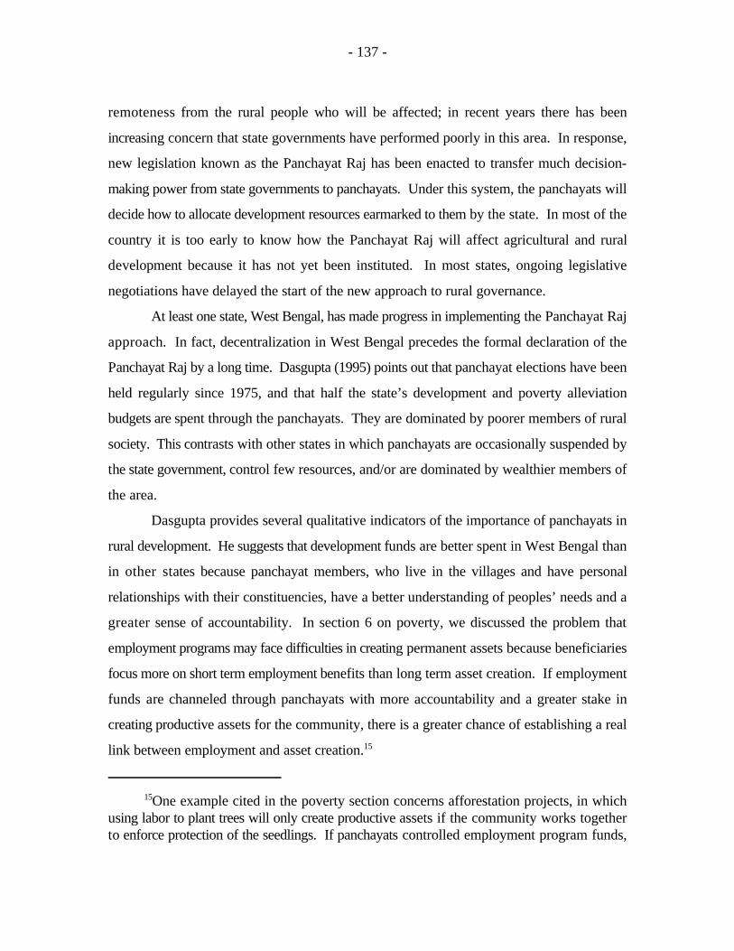
- 137 -
One example cited in the poverty section concerns afforestation projects, in which15
using labor to plant trees will only create productive assets if the community works togetherto enforce protection of the seedlings. If panchayats controlled employment program funds,
remoteness from the rural people who will be affected; in recent years there has been
increasing concern that state governments have performed poorly in this area. In response,
new legislation known as the Panchayat Raj has been enacted to transfer much decision-
making power from state governments to panchayats. Under this system, the panchayats will
decide how to allocate development resources earmarked to them by the state. In most of the
country it is too early to know how the Panchayat Raj will affect agricultural and rural
development because it has not yet been instituted. In most states, ongoing legislative
negotiations have delayed the start of the new approach to rural governance.
At least one state, West Bengal, has made progress in implementing the Panchayat Raj
approach. In fact, decentralization in West Bengal precedes the formal declaration of the
Panchayat Raj by a long time. Dasgupta (1995) points out that panchayat elections have been
held regularly since 1975, and that half the state’s development and poverty alleviation
budgets are spent through the panchayats. They are dominated by poorer members of rural
society. This contrasts with other states in which panchayats are occasionally suspended by
the state government, control few resources, and/or are dominated by wealthier members of
the area.
Dasgupta provides several qualitative indicators of the importance of panchayats in
rural development. He suggests that development funds are better spent in West Bengal than
in other states because panchayat members, who live in the villages and have personal
relationships with their constituencies, have a better understanding of peoples’ needs and a
greater sense of accountability. In section 6 on poverty, we discussed the problem that
employment programs may face difficulties in creating permanent assets because beneficiaries
focus more on short term employment benefits than long term asset creation. If employment
funds are channeled through panchayats with more accountability and a greater stake in
creating productive assets for the community, there is a greater chance of establishing a real
link between employment and asset creation.15

- 138 -
they would recognize this problem and either: 1) ensure that trees were protected, or 2)allocate employment resources elsewhere. Similarly, panchayats could play a critical rolein defining and enforcing collective property rights to groundwater, as discussed in section7.
As an example of panchayats’ legitimacy among rural people in West Bengal,
Dasgupta notes that they play a strong role in dispute resolution even though their actual legal
power is weak. Historically village level disputes, such as over property boundaries, damages
resulting from intrusive grazing, etc., were handled at the village level (Jodha 1980). In
recent years, however, village level institutions have disintegrated, so in many states villagers
settle disputes in distant, state-run courts of law that can take months or even years to reach
decisions. This contrasts sharply with the major role of panchayats in settling disputes in
West Bengal.
Dasgupta points out various weaknesses with the West Bengali panchayat system, but
on the whole, it provides some indication that the Panchayat Raj system may make a strong
contribution to political and economic development in the future.
On the other hand, there is still a shortage of quantitative measurement of the positive
effects of decentralization. Rao and Kalirajan (1995) propose to undertake a study in which
they will use econometric modeling to test the relationship between decentralized governance,
on the one hand, and various development indicators on the other. In addition to the
consistently strong status of panchayats in West Bengal, Andhra Pradesh and Karnataka have
also decentralized, though various changes in state governments have interrupted the
panchayats from time to time. Rao and Kalirajan propose to use district level data for their
analysis and use dummy variables to indicate the districts in West Bengal, Andhra Pradesh and
Karnataka that have had functioning panchayats. The results of this study are not yet
available, but the proposed approach suggests a useful way to address the issue.
Nongovernment Institutions and Weak Local Government. The lack of strong,
credible local government in most states has stimulated the growth of informal committees
and cooperative groups that provide members with important economic and social services.
As discussed in section 6 on poverty and section 7 on watershed management programs,

- 139 -
recent years have seen the spread of informal village level committees and cooperative groups
that provide their members with important economic and social services (Fernandez 1991,
Parthasarathy 1994). Various NGOs are helping villagers organize themselves into self-help
groups that focus on issues ranging from credit to health to watershed management. Informal
thrift groups help their members work collectively to mobilize resources and learn
organizational skills, and they either replace government services too remote from the village
or help link members to them by reducing transaction costs through scale economies.
Clearly, one reason for the appeal of these informal associations is the weakness of
local government. Although such groups would still have a role to play even if local
government were stronger, the fact that it is not increases the demands on such groups. Of
course, while they are able to perform certain important functions, these groups are no
substitute for local government. While they can resolve disputes within a group, for example,
they have no authority and little influence beyond their own membership. And while they can
mobilize meager develop resources of their own members, they have little or no influence on
the allocation of government funds earmarked for village development. Clearly, a strong,
representative local government system is needed to combine the grassroots appeal of
informal groups with the broader powers and authority of government.
Specific Institutional Issues
A few specific institutional concerns affecting agricultural development deserve special
mention.
Credit is well known to play an important role in facilitating investment in improved
agricultural technology. The positive production elasticities for banks in table 9.2 provide
evidence in this regard. Likewise, table 9.3 (from Desai, 1988) shows that, on the whole,
those states with better agricultural performance have a higher volume of short term
production credit per ha.
In most of India, weak formal banking and cooperative systems provide subsidized
credit, but defaults are extremely high and funds are provided disproportionately to relatively

- 140 -
Table 9.3 Comparison of state-wise short-term credit requirement and creditsupply for crop production in 1984-85
Sr. No.
States Supply Requirements Supply toCredit Credit Percent of Credit
Requirement
1. Jammu & Kashmir 5 230 2
2. Himachal Pradesh 5 131 4
3. West Bengal 101 2,959 3
4. Assam 3 870 *
5. Punjab 351 2,118 17
6. Uttar Pradesh 281 3,252 9
7. Bihar 43 1,830 2
8. Orissa 87 2,172 4
9. Andhra Pradesh 493 2,339 21
10. Haryana 187 1,284 14
11. Rajasthan 119 1,048 11
12. Gujarat 223 1,849 12
13. Madhya Pradesh 185 2,236 8
14. Maharashtra 352 2,776 13
15. Karnataka 259 1,466 18
16. Kerala 429 419 102
17. Tamil Nadu 367 2,298 16
Total 3,490** 29,277 12
* Less than one percent** Short-term credit not adjusted to the concept discussed earlier
Source: Desai, D.K. (1988)

- 141 -
large farmers. In addition, occasional interference by politicians to forgive farmers’ debts only
serve to weaken the banking system. Desai (1988) estimates that, excluding Kerala, the ratio
of credit supply to farmers’ short term credit requirements in India is about 1:10. Meanwhile,
informal village moneylenders provide coverage to a wider range of clients but at very high
rates of interest. Hanumantha Rao and Gulati (1994) indicate that many village moneylenders
borrow from the formal sector at concessional rates in order to relend to their poorer
neighbors at higher rates.
Hanumantha Rao and Gulati suggest that for most farmers, the advantages of
subsidized interest rates offered by the formal sector are far outweighed by the fact that
formal sector funds often are not available due to rationing and bureaucratic hassles. They
suggest that the neediest farmers would be made better off if concessional lending were
abandoned and bank managers were given more autonomy and protection against political
interference. Banking operations could be made simpler and more decentralized in order to
reduce transactions costs of both banks and their clients. Higher interest rates would help
banks become viable credit institutions rather than merely a means for channeling concessional
funds. Under these circumstances, banks could attract deposits, and they would have more
incentive to develop better loan portfolios. In short, this step would help develop greater
professionalism in the banking sector (Hanumantha Rao and Gulati 1994).
Land tenure is another issue in which some reform is needed. As mentioned in the
section on natural resource management, land-to-the-tiller laws have led to a situation in
which tenancy is widespread but unofficial, and leases are limited to a year or two in order
to avoid potential ownership claims by tenants. From a natural resource conservation
perspective, this system makes it likely that tenants’ management decisions will be guided by
short time horizons. Not surprisingly, Pender and Kerr (1996) have found in a village level
econometric study that land under tenancy is less likely to receive soil conservation
investments. This situation might not hold if longer term leases were permitted.
Even aside from natural resource management concerns, freeing the tenancy market
would make it easier for landowners to allocate land to its most productive use. Jodha (1984)
shows that much of the lease market in semi-arid areas comprises plots leased by smaller

- 142 -
farmers to larger farmers. An active lease market enables such farmers, who may lack the
means to cultivate their land in any given year, to earn income from it yet retain full
ownership. In other circumstances, land owned in larger holdings is often kept fallow by
absentees who have lost interest in farming but wish to retain their land as a long term asset
(Kerr and Sanghi 1992). An active lease market would encourage such farmers to lease their
land to be used productively rather than left fallow. Land taxes, meanwhile, would reduce
the value of absentee land holdings and possibly encourage sales by absentees.
PRICE AND TRADE POLICIES
Indian agriculture is subject to a wide range of policies, including export restrictions
ranging from licensing requirements to complete bans for certain products, input and output
price controls, and interstate trade restrictions. We do not provide a detailed description of
economic policies affecting agriculture here. Recent years have seen the realization that
despite heavy subsidies for inputs such as fertilizers, credit and irrigation, most of Indian
agriculture is net taxed, not net subsidized (Gulati et al 1989). Taxation comes in the form
of direct restrictions on interstate and international trade, output price controls, and an
overvalued currency that discriminates against tradable goods sectors such as agriculture.
Within the agricultural sector, policies have been mixed in their impact on irrigated
and rainfed agriculture. Some policies are crop-specific; for example, oilseeds have been
heavily protected in recent years, while cotton has been discriminated against (Gulati et al,
1989). Both have large areas under rainfed conditions.
In other respects, however, irrigated agriculture clearly has been favored. We have
already mentioned the infrastructure bias in favor of irrigated areas and its implications for
agricultural development. In addition, canal irrigation is heavily subsidized; not only do users
not bear the massive investment costs, but the charges they pay are so low they cannot even
cover maintenance costs. Well irrigation investments are almost entirely borne by users, but
operations for most users are heavily subsidized via underpriced electricity to power pumps.
Gulati et al (1989) found that, thanks to subsidies on both canal and tubewell irrigation,
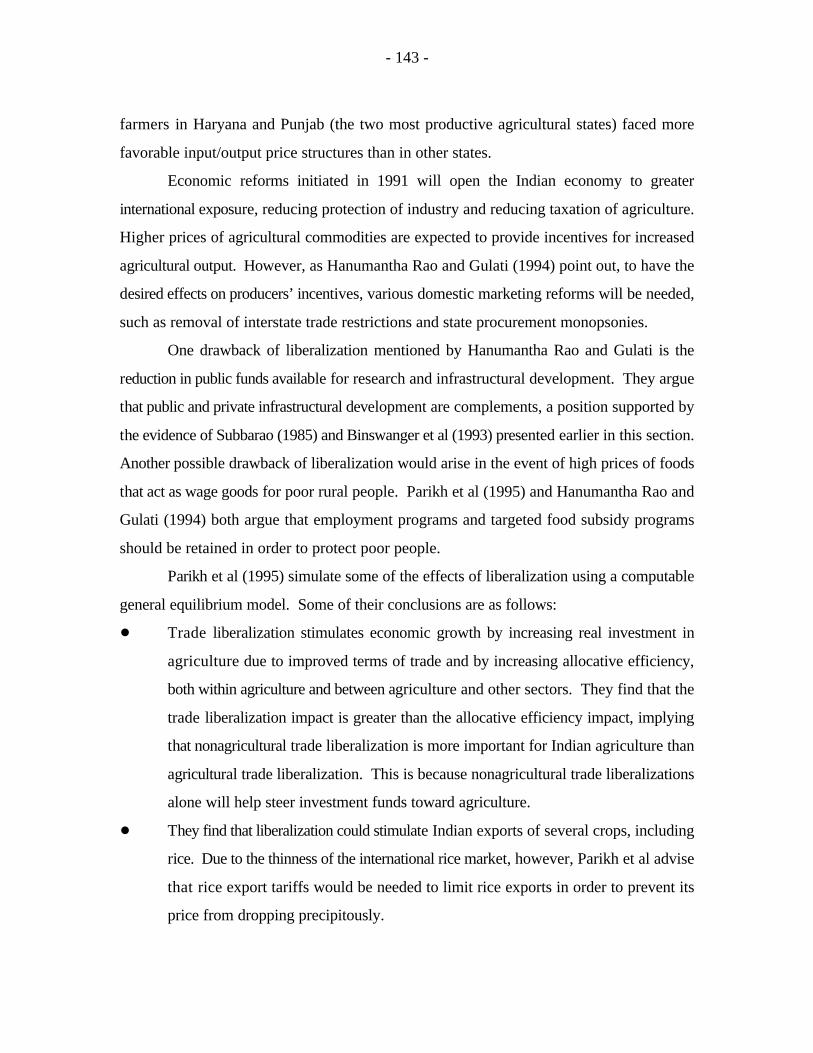
- 143 -
farmers in Haryana and Punjab (the two most productive agricultural states) faced more
favorable input/output price structures than in other states.
Economic reforms initiated in 1991 will open the Indian economy to greater
international exposure, reducing protection of industry and reducing taxation of agriculture.
Higher prices of agricultural commodities are expected to provide incentives for increased
agricultural output. However, as Hanumantha Rao and Gulati (1994) point out, to have the
desired effects on producers’ incentives, various domestic marketing reforms will be needed,
such as removal of interstate trade restrictions and state procurement monopsonies.
One drawback of liberalization mentioned by Hanumantha Rao and Gulati is the
reduction in public funds available for research and infrastructural development. They argue
that public and private infrastructural development are complements, a position supported by
the evidence of Subbarao (1985) and Binswanger et al (1993) presented earlier in this section.
Another possible drawback of liberalization would arise in the event of high prices of foods
that act as wage goods for poor rural people. Parikh et al (1995) and Hanumantha Rao and
Gulati (1994) both argue that employment programs and targeted food subsidy programs
should be retained in order to protect poor people.
Parikh et al (1995) simulate some of the effects of liberalization using a computable
general equilibrium model. Some of their conclusions are as follows:
! Trade liberalization stimulates economic growth by increasing real investment in
agriculture due to improved terms of trade and by increasing allocative efficiency,
both within agriculture and between agriculture and other sectors. They find that the
trade liberalization impact is greater than the allocative efficiency impact, implying
that nonagricultural trade liberalization is more important for Indian agriculture than
agricultural trade liberalization. This is because nonagricultural trade liberalizations
alone will help steer investment funds toward agriculture.
! They find that liberalization could stimulate Indian exports of several crops, including
rice. Due to the thinness of the international rice market, however, Parikh et al advise
that rice export tariffs would be needed to limit rice exports in order to prevent its
price from dropping precipitously.
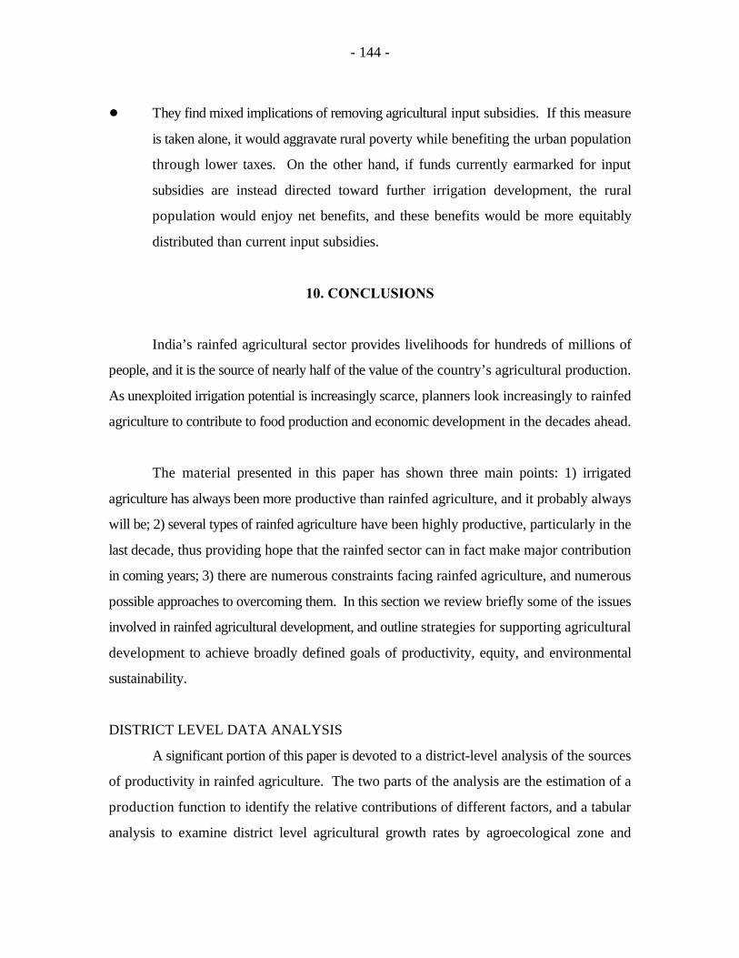
- 144 -
! They find mixed implications of removing agricultural input subsidies. If this measure
is taken alone, it would aggravate rural poverty while benefiting the urban population
through lower taxes. On the other hand, if funds currently earmarked for input
subsidies are instead directed toward further irrigation development, the rural
population would enjoy net benefits, and these benefits would be more equitably
distributed than current input subsidies.
10. CONCLUSIONS
India’s rainfed agricultural sector provides livelihoods for hundreds of millions of
people, and it is the source of nearly half of the value of the country’s agricultural production.
As unexploited irrigation potential is increasingly scarce, planners look increasingly to rainfed
agriculture to contribute to food production and economic development in the decades ahead.
The material presented in this paper has shown three main points: 1) irrigated
agriculture has always been more productive than rainfed agriculture, and it probably always
will be; 2) several types of rainfed agriculture have been highly productive, particularly in the
last decade, thus providing hope that the rainfed sector can in fact make major contribution
in coming years; 3) there are numerous constraints facing rainfed agriculture, and numerous
possible approaches to overcoming them. In this section we review briefly some of the issues
involved in rainfed agricultural development, and outline strategies for supporting agricultural
development to achieve broadly defined goals of productivity, equity, and environmental
sustainability.
DISTRICT LEVEL DATA ANALYSIS
A significant portion of this paper is devoted to a district-level analysis of the sources
of productivity in rainfed agriculture. The two parts of the analysis are the estimation of a
production function to identify the relative contributions of different factors, and a tabular
analysis to examine district level agricultural growth rates by agroecological zone and
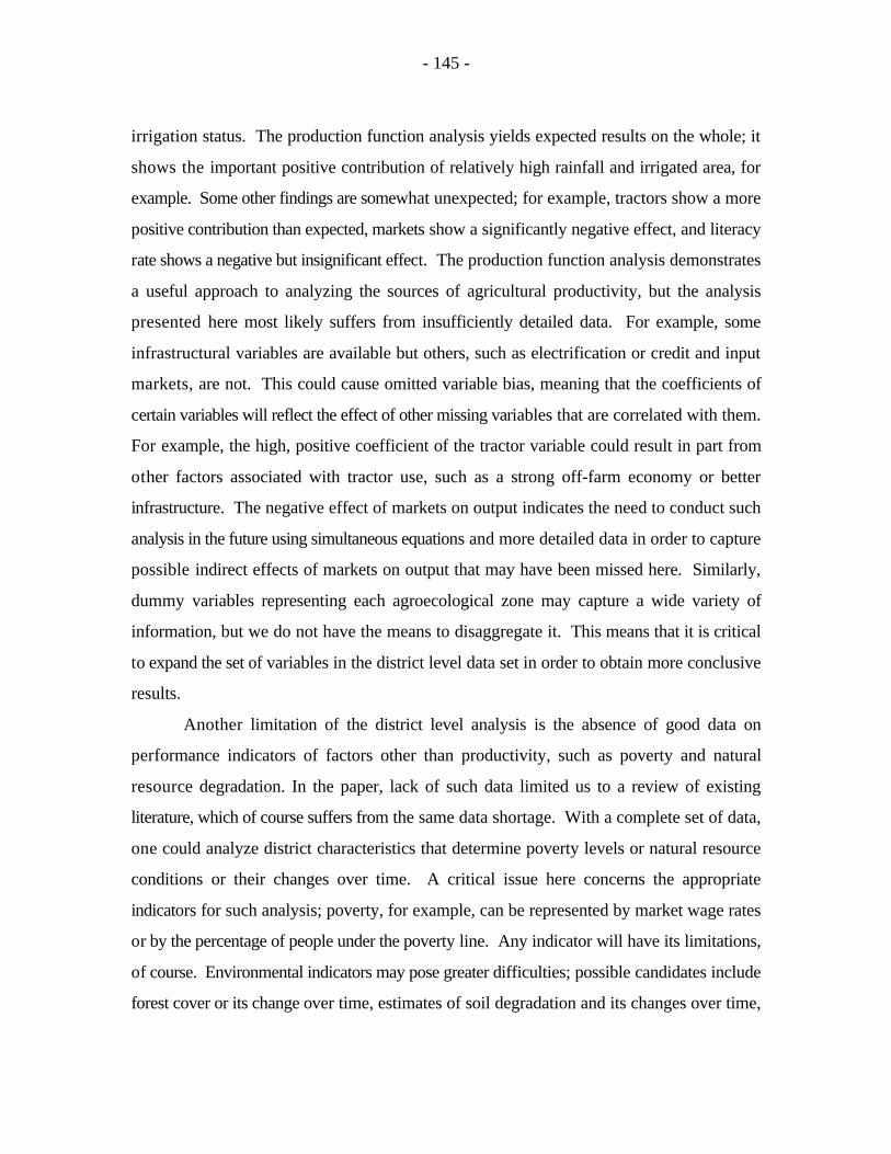
- 145 -
irrigation status. The production function analysis yields expected results on the whole; it
shows the important positive contribution of relatively high rainfall and irrigated area, for
example. Some other findings are somewhat unexpected; for example, tractors show a more
positive contribution than expected, markets show a significantly negative effect, and literacy
rate shows a negative but insignificant effect. The production function analysis demonstrates
a useful approach to analyzing the sources of agricultural productivity, but the analysis
presented here most likely suffers from insufficiently detailed data. For example, some
infrastructural variables are available but others, such as electrification or credit and input
markets, are not. This could cause omitted variable bias, meaning that the coefficients of
certain variables will reflect the effect of other missing variables that are correlated with them.
For example, the high, positive coefficient of the tractor variable could result in part from
other factors associated with tractor use, such as a strong off-farm economy or better
infrastructure. The negative effect of markets on output indicates the need to conduct such
analysis in the future using simultaneous equations and more detailed data in order to capture
possible indirect effects of markets on output that may have been missed here. Similarly,
dummy variables representing each agroecological zone may capture a wide variety of
information, but we do not have the means to disaggregate it. This means that it is critical
to expand the set of variables in the district level data set in order to obtain more conclusive
results.
Another limitation of the district level analysis is the absence of good data on
performance indicators of factors other than productivity, such as poverty and natural
resource degradation. In the paper, lack of such data limited us to a review of existing
literature, which of course suffers from the same data shortage. With a complete set of data,
one could analyze district characteristics that determine poverty levels or natural resource
conditions or their changes over time. A critical issue here concerns the appropriate
indicators for such analysis; poverty, for example, can be represented by market wage rates
or by the percentage of people under the poverty line. Any indicator will have its limitations,
of course. Environmental indicators may pose greater difficulties; possible candidates include
forest cover or its change over time, estimates of soil degradation and its changes over time,
- 146 -
etc. The tremendous diversity of natural resources over small areas may suggest that the
district is actually too large a unit for such analysis, because different parts of a district may
face different kinds of problems. Researchers at ICRISAT and the Indo-Swiss Livestock
Project have recently used mandal level data to analyze crop and livestock production
patterns in Andhra Pradesh; this may prove to be a more appropriate level of analysis for
certain problems. As in all socioeconomic research, the utility of using the more
disaggregated data depends on the additional costs of collecting it and the additional benefits
of the information that it is expected to yield.
The tabular analysis was designed to provide a disaggregated analysis of growth rates
over time under different conditions. Other studies have conducted the same analysis on an
aggregated scale, for example to compare agricultural growth in predominantly irrigated vs
predominantly rainfed districts, or to compare agricultural growth before and after the green
revolution. Our analysis also does this, and it agrees with other studies that growth rates have
been roughly constant over the entire period. Our study further attempts a more
disaggregated analysis in order to identify the sources of growth in different periods. This
approach can help us examine, for example, whether irrigated wheat regions drove growth
in the first 10-15 years of the green revolution but favorable rainfed areas drove growth
subsequently. Our study also disaggregates rainfed agriculture into different types, unlike
other studies. This enables us to identify variations in the performance of rainfed agriculture
on the basis of region and other characteristics.
Our analysis does not show conclusive results regarding changes in the sources of
growth over time. One reason for this may be that in tabular analysis, the data cannot be
disaggregated perfectly, and somewhat arbitrary decisions are required to classify districts by
irrigation status and to delineate time periods. More persistent efforts to analyze the data
under alternate specifications of time periods and irrigation status may or may not result in
more striking findings.
Our analysis also does not show conclusive evidence regarding the determinants of
growth for different rainfed agricultural types. The tabular analysis shows that rainfed
agriculture has grown slowest in the green revolution areas of the northwest, where irrigated

- 147 -
agriculture has driven large increases in overall food production. Rainfed agriculture grew
at less than 1% during the period 1968-84, and less than 2% in the period 1984-91. In the
rest of the country, rainfed agricultural production grew at rates of 1.4% to 3.5% percent
during the period 1968-84, and 2.9% to 4.7% between 1984 and 1990 (table 4.1). The
production function analysis is designed to help explain the factors that drive these variations.
It shows that rainfall levels are perhaps the most important determinant; it also supports the
point made by earlier researchers that differences in the level of infrastructure (particularly
roads) help determine rainfed agricultural growth rates. However, the data are insufficiently
detailed to provide a more definitive picture of the causes of variations in growth rates for
different rainfed agricultural types. Subsequent analysis will address this question.
SPECIFIC ISSUES
Agricultural Research and Extension
Evidence suggests that public and private sector agricultural research efforts have
been highly successful in developing seed technology that is widely adopted and highly
productive in irrigated areas and favorable rainfed zones. The strong performance in recent
years of rainfed rice in eastern India and rainfed sorghum in central India provide the basis for
optimism that rainfed agriculture can in fact be an important source of agricultural production
in the coming decades.
For soil and water management technology in these areas and for all kinds of
agricultural technology in unfavorable rainfed areas, however, agricultural research has had
limited impact. Evidence suggests that the current approach of developing technology
packages on research stations and then transferring them to farmers’ fields has had limited
effectiveness. This is the case for two reasons. First, the diversity of rainfed agricultural
systems may require location specific approaches to soil and water management, so that a
single system developed in isolation on a research station may not be widely applicable.
Second, farming systems in marginal areas are highly diversified, and they coexist with other
nonagricultural activities that comprise a household’s livelihood strategy. As a result, new
- 148 -
land management technologies developed on research stations may interfere with other
components of existing farming systems. If this is so, then adopting the new technologies
imposes opportunity costs on farmers who must adapt or sacrifice other components of their
existing farming systems, which of course makes the new technologies less attractive. This
implies the need for more diagnostic work to understand farming systems better. It also
suggests that developing new technology in participation with farmers, building on their
existing farming systems to improve soil and water management, may yield new technologies
that are both effective and widely adopted.
The extension system faces a similar set of challenges. The extension system
traditionally has followed a one-way system of communication; it transfers technology
developed on research stations to farmers. There is no formal system for reversing the flow
of communication, so scientists are rarely in direct correspondence from farmers in order to
receive specific, detailed reactions to the new technologies developed. The extension system
may become more effective if it serves as a channel for more effective two-way
communication between farmers and researchers. Similarly, the extension system can benefit
from increased farmer-to-farmer extension. This is the case for two reasons. First, farmers
are likely to understand each other’s objectives and constraints better than outsiders, so they
can communicate more effectively. Second, the large discrepancies in agricultural
productivity within villages may suggest that there may be significant scope for transferring
knowledge from more productive farmers to their neighbors. Much of the difference may be
attributable to differences in soil types and other constraints, but some evidence suggests that
differences in technical knowledge also matter.
Irrigation
One obvious approach to developing agriculture in rainfed areas is to expand the area
under irrigation. Irrigation is the agricultural investment of choice among private farmers in
semi-arid areas (Pender 1993), and as we have seen, irrigation enables farmers to achieve
higher, more stable yields. Irrigation development, however, can never be more than a partial
solution to the problems of agricultural development, because total irrigation potential is only

- 149 -
sufficient to irrigate about half of the total cultivated area. The rest will remain rainfed.
Nevertheless, it is important to continue to develop new sources of irrigation and improve the
economic and technical efficiency of existing irrigation capacity. Equity and environmental
sustainability also are critical issues in irrigation development. The major issues are as
follows:
! In many water scarce areas, groundwater capacity is nearly fully utilized; additional
wells cause water tables to fall, in some cases depleting aquifers or leading to
saltwater intrusion. In large part, this problem results from the low, flat rate charged
for electricity to power wells and the lack of property rights assigned to groundwater.
Serious efforts are needed in water scarce areas to link pumping charges to the
volume pumped, and to develop effective property rights to groundwater. Little
effort has been made in reforming power prices and water property rights, but there
is growing awareness of the problems and some movement toward developing
solutions.
! The status quo in well irrigation in dry areas potentially is highly inequitable, since
it favors farmers who can afford to continually deepen existing wells or dig new ones.
Water markets are a mitigating factor that enable farmers without wells to enjoy the
benefits of groundwater. Groundwater markets have developed rapidly in some areas
but slowly in others, and their competitiveness varies as well. Shah (1993) has
shown that water buyers receive the most favorable prices when electricity is charged
at a flat rate, but in dry areas this pricing system leads to overexploitation of the
resource (Kerr et al 1996). Additional work is needed to see how to further develop
water markets in dry areas in ways that are both equitable and environmentally
sustainable.
! Protective or supplementary irrigation of dryland crops is potentially a powerful
mechanism to spread the benefits of irrigation over a much larger area and to
increasing numbers of farmers (Dhawan 1988b). Many dryland crops show
substantial yield increases resulting from one or two protective irrigations, yet in many
water-scarce regions, irrigation water is used intensively for such crops as paddy,
- 150 -
sugarcane and horticultural crops, while dryland crops remain purely rainfed. Further
work is needed to understand the private and social costs and benefits of extensive vs
intensive irrigation, the circumstances under which farmers practice one as opposed
to the other, and policy tools that can be taken to encourage the most efficient use of
irrigation water.
! Groundwater irrigation is less developed in many more favorable rainfed areas, such
as eastern India. This is partly due to the fact that water is less limiting to crop
production in such areas, but also possibly to complex tenure relations that inhibit
long term land improvement investments such as wells (Repetto 1994). Irrigation
development would increase dry season cultivation in these areas, with potentially
strong implications for increased production. More work is needed to assess private
and social net benefits of well investment in these areas and constraints to socially
optimal investment.
! In canal irrigated areas, the area that actually receives irrigation water can be
increased through better management of canals that leads to a greater transfer of
water from “front end” to “tail end” water users. Engineering and social organization
solutions can be combined to organize water users into smaller, more cohesive groups
in order to facilitate more efficient and equitable distribution of irrigation water.
Sustainable Use of Fragile Lands
Much of the effort devoted to increased productivity of rainfed agriculture revolves
around land use planning for integrated use of different types of land. Watershed development
is the vehicle by which improved land use principles are promoted. Several problems plague
the concept of improved land use, and various steps are needed to solve them.
! According to ICAR, large areas of land are used in ways that are inconsistent with
their capability; for example, sloped plots with shallow soil are used to grow field
crops even though perennial vegetation is recommended to reduce soil erosion and
build up soil nutrients. While unsustainable land use is undoubtedly widespread, it is
worth studying indigenous farming systems to make sure we understand them well

- 151 -
enough to know their sustainability implications. In many cases farmers do undertake
steps to protect resources, but outsiders do not recognize them as such because they
do not resemble practices developed by scientists (Kerr and Sanghi 1992). Often
understanding a natural resource management system requires observing it in a
dynamic context, since what we see in a single point in time may be misleading. For
example, many farmers in hilly areas deliberately induce erosion within their plots in
order to encourage natural terracing. A casual observer visiting the site in its erosion
stage might miss the point.
! Similarly, where farmers are using land unsustainably, there is a need to understand
better why they do so. Understanding the determinants of land use is needed to
identify the constraints to change, and thus to developing effective, adoptable
alternatives. For example, often the argument is made that farmers use
environmentally damaging practices because they do not know any better, or because
they are too poor to be concerned about sustaining future productive capacity. On
the other hand, a growing body of evidence suggests that farmers do perceive
environmental degradation and know how to reduce or prevent it, and that
inappropriate policies and institutions may be more to blame than ignorance or
poverty in leading to degradation. Examples in the Indian context include soil erosion
and the adoption of measures to prevent it, and the management of various common
property resources.
! Watershed management projects provide a useful context for identifying the
conditions under which farmers are or are not willing to adopt recommended
practices. Technology transfer in most watershed projects has been so heavily
subsidized, however, that it is extremely difficult to learn whether farmers accept
technology for its own sake or simply to obtain subsidy benefits. Watershed projects
also present a means for experimenting with alternate approaches to technology
development and social organization leading to more efficient and sustainable land
use. But most projects are managed so inflexibly that inhabitants have little say
regarding the design and implementation of project interventions. They are also

- 152 -
heavily oriented toward promotion of new technology. Yet evidence from around the
world shows that cases of sustainable rural resource management have relied not on
externally introduced technology but rather sound economic policies, infrastructure
and institutions that give villagers the incentive to manage natural resources better and
encourage them to put their existing knowledge to better use. Watershed projects so
far have been an unexploited opportunity for developing innovative approaches to
land use, both at the individual and community levels.
! The district level analysis was not able to address issues related to environmental
degradation because the data were inadequate for the task. Environmental indicators
have two kinds of shortcomings. First, rarely are they available on a district level
basis, and second, many are not available on a historical basis, making it difficult to
relate their changes over time to possible causal factors. Soil degradation is a good
example; the NBSS&LUP in Nagpur has recently mapped the erosion status in
various regions of the country, but the data are not matched to districts. With some
effort this could be done on a very rough basis, but only for one period in time (the
early 1990s). Some data, such as changes in approximate area covered by forests or
percent of groundwater utilized, could be constructed for at least some part of the
period under study. Additional efforts to construct such data may be useful. On the
other hand, in some cases diversity of natural resource condition might justify the use
of a smaller scale of analysis, such as the taluk or mandal. Likewise, under this
approach analysis could be undertaken even if data are available only from a few
states.
District- or even mandal-level data can be critical for analyzing some
determinants of natural resource management, such as different institutional or legal
approaches or the effects of pricing and marketing policies. However, village and
household studies also are needed to understand people’s knowledge about natural
resource management and mechanisms by which they make decisions. A balance
between more aggregated studies that yield “big-picture” trends and village-level
studies that yield the details of how decisions are made is needed to understand what

- 153 -
drives environmental degradation and devise policies and institutions needed to
reverse it.
Infrastructure
The few studies available on infrastructure suggest that it has a strong positive impact
on agricultural development, and that government infrastructure investments are concentrated
in more favorable agroclimatic areas. The analysis in this study showed little if any effect of
roads and regulated markets, the two infrastructural variables available, on agricultural
output. However, this may be due to insufficient disaggregation of the data. Infrastructure,
like environment, is a subject on which additional district level variables are needed to
facilitate more detailed analysis of its contribution to agricultural development. In the present
analysis, the data on kilometers of roads and the number of regulated markets in a district may
(or may not) be correlated with other types of infrastructure such as access to credit, specific
inputs, or public transportation, for example. In any event, it would be beneficial to conduct
the district level analysis with more detailed infrastructural data that captures 1) more types
of infrastructure and 2) its quality.
Additional types of infrastructure might include health and educational facilities,
formal and informal credit sources, electrification, and extent of public transportation, to
name a few. More importantly, the quality of infrastructure is critical to whether it stimulates
the economy. Formal credit services, for example, are well known to ration credit, so a
variable such as the number of banks may indicate nothing about poor people’s access to
credit. The number of markets, likewise, may not indicate whether agricultural inputs are
available to all who need them on a timely basis. All types of infrastructure are subject to
similar questions about quality -- do schools attract students or teach them anything? Does
the current run in electrified villages? Indicators of the quality of infrastructure may be
difficult to obtain, in which case proxies may be sought. The presence of the Integrated Rural
Development Program (IRDP) or other such schemes may give an indication of widespread
access to credit or inputs, for example. Perhaps the best indicator of access to credit is the
prevailing market rate of interest from informal sources, but this information would be

- 154 -
available only through village-level data. Quality indicators for other kinds infrastructure,
such as delivery of electricity or petroleum-based energy, perhaps may be obtained from
appropriate state government offices.
Decentralization and Local Institutional Development
In many respects, decentralization and local level institutional development are the
“hot item” expected to overcome numerous constraints to agricultural and rural development.
Both theory and experience support arguments in favor of rural infrastructural development,
but it is too early to know what will happen as India embarks on the Panchayat Raj
decentralization plan. The concept behind decentralization is that local governments will be
more aware of local problems and peoples’ priorities, and that they will have more at stake
in delivering high quality service. State government planners, on the other hand, cannot be
expected to have as clear an understanding of local concerns, nor are they as accountable to
specific constituents in remote areas. Evidence in favor of this view is limited, coming mainly
in the form of 1) the positive experience of strong panchayat government in West Bengal and
2) the rise of informal local organizations, such as thrift groups and natural resource users’
groups, that have helped their members raise funds or promote collective action, among other
things.
Some observers believe that the local groups’ informality is their greatest strength.
By remaining small, with a limited agenda, they can focus on issues of specific interest to the
group, which is defined by the homogeneity and common interests of its members. These
groups may select their own members and are accountable to and controlled by only
themselves, which simplifies their operation. Neither government bureaucracy not local elites
can do much to obstruct them. For these reasons, a formal local government system may not
be able to duplicate their strengths.
Others, meanwhile, suggest that the logical step to follow the positive experience of
informal local organizations is to develop formal, institutionalized local organizations with
authority extending beyond the group. The panchayat would embody this approach.
Proponents anticipate that it will combine the advantages of local participation and

- 155 -
organization with access to government resources and real authority over how they are
allocated.
Of course, even if panchayats cannot duplicate all the advantages of informal
organizations, there is no reason the two cannot coexist. In fact, informal groups may
become more effective under the Panchayat Raj system because they can more easily influence
a government that operates at the local level as opposed to the state capital.
Whether the Panchayat Raj will be able to stimulate rural development will depend
ultimately on the quality of governance by panchayat bodies. Will local government be truly
representative and address development objectives of a broad spectrum of the rural
population, or will it be dominated by local elites, so that they be in a better position than ever
to channel funds and other resources in their favor? The semi-feudalistic history of rural India
makes it easy to envision the latter scenario. Information is probably available on
determinants of the quality of local governance, but it was not available for this study. In any
event, some steps will be needed to nurse the panchayat system to become a healthy, mature
democratic institution.
It is important to point out that the Panchayat Raj and other institutional
innovations, such as Joint Forest Management, indicate that the central government is
committed to diffusion of authority to the local level. This process can only be expected
to move gradually, but evidence suggests that it is certainly moving. In time, many other
institutional innovations may follow from the emergence of the Panchayat Raj; for example,
it may spawn new mechanisms for managing common property natural resources such as
groundwater.
Other Issues
Price policy reforms are underway and are likely to have a favorable effect on
agriculture relative to other sectors. The limited evidence is mixed regarding the likely
relative impact on rainfed and dryland crops; the effect will depend largely on the crop in
question. Oilseeds, which are grown widely under rainfed conditions, are protected and will
become less favorable under price reforms, while cotton has been taxed will become more
- 156 -
favorable with reforms. Additional research currently underway at ICRISAT and NCAER
is expected to provide information about the likely effects of reforms on other crops.
Technical assistance, information dissemination, and income support measures may be needed
to help farmers in the transition from crops that become less favorable to others that become
more favorable.
Production risk. Although the unreliable weather in many rainfed areas causes
growing conditions and yields to vary greatly across years, farmers have developed various
coping strategies to insulate themselves from income risk, at least to a certain degree. As a
result, even if individual crop yields vary greatly across years, farmers’ incomes may not, so
increased yield variability of HYVs is not necessarily a deterrent to adoption. Moreover,
research on improved pearl millet seeds shows that high yielding hybrids will often be superior
to traditional varieties even under poor rainfall conditions, implying that higher expected yield
does not necessarily translate to greater yield risk.
Farmers’ drought management strategies fail, however, in the event that widespread
drought causes crop failure over a wide area and depresses the rural economy so much that
all sources of income are affected. Such aggregate level, covariate risk calls for government
intervention to help stabilize incomes and prevent famine. Rural employment and food
subsidy programs deserve credit for reducing drought-related hunger in India in the last two
decades. On the other hand, government-sponsored rainfall insurance schemes have probably
not contributed to increased adoption of improved seeds, but they have done a great deal to
drain public funds.
Poverty alleviation programs can play an important role in supporting the poorest
rural people, and they have the potential to help mitigate the effects of price reforms on those
people whose incomes will fall with reforms. Poverty alleviation programs enjoy widespread
political support, but they face two challenges: 1) to operate in as cost-effective a manner as
possible, and 2) to stimulate the creation of long term development assets. Many observers
argue that employment programs represent the best way to achieve these objectives while also
alleviating poverty, but only under certain conditions. Most importantly, they should offer
wages slightly below the prevailing market wage in order to attract people who really need
- 157 -
assistance and to minimize distortions in the rural economy. Second, using employment
programs to create long term assets is more complicated than it first appears; in many cases
only illusory assets are created (Jackson 1982; Kerr et al 1994). As a result, such programs
should be developed only after experimentation on a small scale yields an understanding of
their ability to create long term development assets.
Human capital development is often mentioned as a critical step toward stimulating
the rural economy. Educated farmers can more easily process information and thus are
prepared to make better decisions; they also may contribute to the diversification of the local
economy, because they will have more to offer to a variety of nonfarm economic activities.
Walker and Ryan (1990) show that household level education is negatively correlated with
poverty; Hazell and Singh 1993 find the same. Also, better educated farmers may impose
pressure on government to be more accountable to its constituents and serve them more
effectively.
The production function analysis in this study provided counterintuitive results
regarding the contribution of literacy to the value of agricultural output. The reason for the
negative relationship found between the two is not clear; perhaps it is simply an anomaly of
the data resulting from the fact that many infrastructural and institutional variables are not
available.
Despite the findings of our analysis, it seems reasonable to argue in favor of increased
investment in education in rural areas. Education will contribute to economic diversification,
which probably represents the long term solution to development of less favorable areas, and
it will contribute to declining rates of growth in the population.
Tradeoffs Between Investments in Different Types of Agriculture
One of the questions motivating this study concerned the likely returns and tradeoffs
involved in diverting development resources from more favorable to less favorable areas.
Unfortunately the quantitative analysis did not shed much light on this subject, but the review
of existing literature offers some useful insights.

- 158 -
Binswanger et al (1993) provide evidence that more favored areas receive more
infrastructure investment, which in turn creates further regional disparities. Their finding of
the positive impact of infrastructure may suggest that areas with less developed infrastructure
will have higher marginal returns to additional investment, in which case shifting resource
allocation in favor of less developed areas would be more efficient as well as more equitable.
More decentralized infrastructural investment allocation under the Panchayat Raj may lead
to less biased allocation between regions, as long as funds are distributed equitably among
panchayats.
Other recommendations listed above argue for changes in the way problems are
addressed, but they may not have major implications for interregional or intersectoral resource
allocation. Agricultural research in marginal areas provides a good example. As shown in
section 4, there is no bias against marginal areas in the allocation of resources for agricultural
research, and no strong argument in favor of shifting resources from favorable to marginal
areas. Instead, the main argument presented here regarding the allocation of research
resources in marginal areas is that there should be a shift in emphasis toward on-farm research
and toward solutions based increasingly on social organization, not just technology. The shift
in resource allocation that this would imply is strictly within the region and the sector, not
between sectors. The key challenge is to change the culture of agricultural research to
overcome the aversion to working in farmers’ fields and the perception that farmers have little
to offer the research process. This challenge is by no means trivial. Researchers need
stronger incentives to conduct more on-farm work. In many cases they will need help in
building collaborative arrangements with people, such as extension workers or NGO officials,
for example, who can help bring them in contact with farmers.
As mentioned above, there is a distinct trend toward the view that the solutions to
rural problems lie with rural people. The introduction of Joint Forest Management and the
Panchayat Raj provide strong evidence of this shift. Meanwhile, gradual movement is taking
place toward more participatory approaches to watershed management, technology
development, and other activities. Truly participatory approaches are still in the minority, but
they are less frequently treated as anomalies. Government projects are increasingly
- 159 -
attempting to become participatory in nature, and although their progress is slow, it is also
steady.
Steps toward Increased Participation of Rural People
As with most problems, it is easier to diagnose shortcomings than to prescribe
solutions. Agricultural development is prone to fads, in which recommendations come in
style with little solid evidence of their worth and then eventually go out of style. In this paper
the main strategy argued for is more decentralization and participation in planning and
developing infrastructure, institutions, and technology. While there is growing evidence of
the advantages of participatory approaches to research and development, it remains fairly
scattered and anecdotal. In India, most of the evidence comes from the voluntary sector, and
much of it is not well documented. Agricultural researchers and development project
managers in the government sector do not have ready access to this material, and there is little
incentive for them to try to obtain it. In recent years participation has become a “buzz word”
in development circles, and many government projects have paid lip service to the term.
However, they are not truly participatory because local people still have little or no influence
in project planning and implementation. Meanwhile, government officials exposed to these
projects may rightly argue that the so-called participatory approach has not yielded any
particular benefits, and participation will have a bad name. This is the surest way to turn
participatory development into a passing fad.
Efforts are needed to expose more scientists, planners and project managers to truly
participatory methods and train them in their use. This should be done incrementally, for
several reasons. First, arguments in favor of greater participation are based on relatively
limited experience, and they require further testing in the field before embarking on them in
full force. Special grants may be made available to researchers interested in pursuing on-farm
research, or to project planners who wish to try new approaches on a small scale. It is
important to note that ICAR tends to promote research that follows fairly strict
methodological guidelines which, incidentally, do not favor participatory research. Various
government ministries organize development projects in the same manner: large scale

- 160 -
programs follow strict implementation guidelines, with little flexibility for experimenting with
project design. The resulting “all-India coordinated project” approach inhibits testing ideas
that fall outside the realm of the specific guidelines. Moreover, such a rigid approach means
that when project guidelines change, they apply to everyone. Radical changes in project
guidelines would be highly risky, in case the new approach does not work. A better approach
would be to build flexibility in project design, so that some special, small scale projects are
allowed to try new approaches. Researchers and project managers working under such
circumstances would have to adapt to a variety of local conditions, and they would have to
be willing and able to accept and learn from feedback from farmers.
A second reason why participatory approaches should be implemented gradually is
that researchers and development planners cannot be transformed overnight. People have
spent entire careers in these fields without ever seriously seeking input from local people, so
change will come gradually. Special grants for participatory projects would attract creative,
field-oriented researchers and project managers. Their more conservative colleagues could
observe their work and be influenced accordingly.
A third, important point is that some problems are more suited to participatory
approaches than others. In agricultural research, for example, traditional research-station
approaches are highly suited to activities such as mapping plant genes or analyzing soil
chemical and physical processes, for example. The argument in favor of increased
collaboration between scientists and farmers is not an effort to dismantle the existing research
system. Rather, it is an effort to change the culture of research so that scientists understand
problems from farmers’ perspectives and design technologies that are more applicable to
farmers’ conditions.
- 161 -
REFERENCES
Agarwal, B. 1992. Rural women, poverty and natural resources: sustenance, sustainabilityand struggle for change. In Poverty in India: Research and Policy, eds. B. Harriss, S.Guhan and R Cassen. New Delhi: Oxford University Press.
Aggarwal, Rimjhim. 1995. Collective Action in Small Groups: The Case of Group OwnedWells in India. Department of Agricultural and Resource Economics, University ofMaryland.
Ahluwalia, Deepak. 1995. Agricultural Growth in India: Trends, Sources and Challenges.(draft). New Delhi: World Bank.
Allison, F.E. 1973. Soil Organic Matter and Its Role in Crop Production. Amsterdam:Elsevier.
Anderson, Jock, and Peter Hazell. 1989. Variability in Grain Yields. Baltimore: JohnsHopkins.
Anderson, Jock, and Peter Hazell. 1994. Risk considerations in the design and transfer ofagricultural technology. In Agricultural Technology: Policy Issues for the InternationalCommunity, ed. Jock Anderson. Wallingford, UK: CAB International.
Bapna, S.L., H. Binswanger, and J. Quizon. 1984. Systems of output supply and factordemand equations for semi-arid tropical India. Indian Journal of Agricultural Economics39 (2): 179-202.
Basu, D.N. and S.P. Kashyap. 1992. Rural nonagricultural employment in India: Role ofdevelopment process and rural-urban employment linkages. Economic and PoliticalWeekly (December 19).
Basu, A.K., Narayan, S.S., and P. Singh. 1992. Cotton Production and Improvement inIndia. Agricultural Situation in India 47 (5).
Bentley, William R. 1984. The uncultivated half of India: Problems and possible solutions.Discussion Paper No. 12. New Delhi: Ford Foundation.
Bidinger, Patricia D., T.S. Walker, B. Sarkar, A. Ram Murthy, and P. Babu. 1990.Economic, health, and nutritional consequences of the mid-1980s drought on a tank-irrigated, Deccan village in South India. Economics Group Progress Report No. 98.Patancheru, India: ICRISAT.
Binswanger, Hans. 1978. The Economics of Tractors in South Asia: an Analytical Review.New York: Agricultural Development Council and Hyderabad, India: ICRISAT.

- 162 -
Binswanger, H. and B. Barah. 1980. Yield risk, risk aversion, and genotype selection:Conceptual issues and approaches. Research Bulletin No. 3. Hyderabad, India:ICRISAT.
Binswanger, Hans P., Shahidur R. Khandker, and Mark Rosenzweig. 1993. How infra-structure and financial institutions affect agricultural output and investment in India.Journal of Development Economics 41 (2) (August).
Bowonder, B. and C. Ravi. 1984. Waterlogging From Irrigation Projects: AnEnvironmental Management Problem. Hyderabad: Centre for Energy and Technology,Administrative Staff College of India.
Byerlee, Derek. 1992. Dryland wheat in India: The impact of technical change and futureresearch challenges. Economics Working Paper No. 92-05. Mexico City: CIMMYT.
Byerlee, D. 1994. Technology transfer systems for improved crop management: Lessons forthe future. In Agricultural Technology: Policy Issues for the International Community,ed. J.R. Anderson. CAB, Wallingford, UK.
Chambers, Robert, N.C. Saxena, and Tushaar Shah. 1989. To the Hands of the Poor: Waterand Trees. New Delhi: Oxford and IBH.
Chhibber, A. 1988. The aggregate supply response in agriculture: A survey in S.Commander. In Structural Adjustment in Agriculture: Theory and Practice in Africa andLatin America. London: James Curry.
Cogle, A.L., and K.P.C. Rao. 1993. Water conservation in soils of the semi-arid tropics.Proceedings of the International Symposium on Agroclimatology and SustainableAgriculture in Stressed Environments. Hyderabad: ICAR/ICRISAT.
Cogle, A.L., M. Littleboy, K.P.C. Rao, G.D. Smith and D.F. Yule. 1996. Soil managementand production of alfisols in the semi-arid tropics. Part III: Long-term effects on waterconservation and production. Australian Journal of Soil Research 34.
Dantwala. 1986. Agrarian structure and agrarian relations in India. In Indian Society ofAgricultural Economics: Indian Agricultural Development Since Independence.Bombay: Oxford University Press and IBH Publishing Co.
Dasgupta, Biplab. 1995. Institutional reforms and poverty alleviation in West Bengal.Economic and Political Weekly (October 14-21).
Desai, B.M. 1994. Raising agricultural output: price and nonprice factors. Finance andDevelopment (June).
- 163 -
Desai, D.K. 1988. Institutional credit requirements for agricultural production-2000 AD,Indian Journal of Agricultural Economics 43 (3).
Desai, G.M. 1982. Sustaining rapid growth in India’s fertilizer consumption: A perspectivebased on composition of use. Research Report No. 41. Washington, DC: IFPRI.
Desai, G.M. 1985. Market channels and growth of fertilizer use in rainfed agriculture:Conceptual considerations and experience in India. In Agricultural Markets in theSemi-arid Tropics. Proceedings of the International Workshop (October 24-28, 1983).Patancheru, India: ICRISAT.
Desai, G.M., and S. Rustagi. 1994. Agricultural Growth in India: A Perspective Based onAgro-Climatic Regions. Washington: IFPRI.
Dhawan. B. 1988a. Irrigation in India’s Agricultural Development. New Delhi: Sage.
Dhawan. B. 1988b. Dryland versus irrigated farming. Economic and Political Weekly(March 19).
Dholakia, R.M., and B.M. Dholakia. 1993. Growth of total factor productivity in Indianagriculture. Indian Economic Review 28 (1).
Dhruvanarayana, V.V., and Ram Babu. 1983. Estimation of soil erosion in India. Journalof Irrigation Drainage Engineering. ASCE 109 (4).
Dhyani, B.L., Ram Babu, Sewa Ram, V.S. Katiyar, Y.K. Arora, G.P. Juyal and M.K.Vishwanatham. 1993. Indian Journal of Agricultural Economics 48 (2) (April-June).
Dregne, Harold E., and Nan-Ting Chou. 1992. Global desertification: Dimensions and costs.In Degradation and Restoration of Arid Lands, ed. Harold E. Dregne. Lubbock, Texas:Texas Tech University.
Dvorak. 1988. Indigenous soil classification in semi-arid tropical India. Economics GroupProgress Report No. 84, Resource Management Program. Patancheru: ICRISAT.
Dvorak, 1992. On-farm experiments as a diagnostic method: Constraints to nitrogenfertilizer use on sorghum in semi-arid tropical India. Experimental Agriculture 28 (2)(April).
El-Swaify, Samir E., W. Dangler and C.L. Armstrong. 1982. Soil Erosion by Water in theTropics. Honolulu: College of Tropical Agriculture and Human Resources, Universityof Hawaii.

- 164 -
Evenson, Robert. E., Carl. E. Pray and Mark. W. Rosegrant. 1996. Agricultural researchand productivity growth in India. Research Report (Forthcoming), Washington, DC:IFPRI.
Fernandez, A.P. 1991. The MYRADA Experience: Alternate Management Systems forSavings and Credit of the Rural Poor. Bangalore: MYRADA.
Fernandez, A.P. 1993. The MYRADA Experience: The Interventions of a Voluntary Agencyin the Emergence and Growth Peoples' Institutions for Sustained and EquitableManagement of Micro-watersheds. Bangalore: MYRADA.
Fujisaka, J.S, K.T. Ingram, and K. Moody. 1991. Crop establishment (Beusani) in CuttackDistrict, India. IRRI Research Paper Series No. 148. Los Banos, Philippines: IRRI.
Gadgil, Madhav. 1982. Forest Management and Forest Policy in India: a Critical Review.In Forests, Environment and People, ed. Fernandes, Walter. New Delhi: Indian SocialInstitute.
Gadgil, Madhav, and Ramachandra Guha. 1992. This Fissured Land: An Ecological Historyof India. New Delhi: Oxford University Press.
Gill, G.J. 1995. Major natural resource management concerns in South Asia. Prepared forthe Conference on a 2020 Vision for Agriculture. Washington, DC: IFPRI.
GOI. 1976. Report of the National Commission on Agriculture, Part IX: Forestry. Ministryof Agriculture and Cooperation, Government of India, New Delhi.
Gulati, Ashok, with James Hanson and Garry Purcell. 1989. Effective incentives in India’sagriculture: Cotton, groundnuts, wheat and rice. New Delhi: World Bank.
Gupta, Anil. 1989. Scientists’ views of farmers’ practices in India: Barriers to effectiveinteraction. In Farmer First: Farmer Innovation and Agricultural Research, RobertChambers, Arnold Pacey and Lori Ann Thrupp. London: Intermediate TechnologyPublications.
Gupta, Anil. 1991. An Alternative Approach to Development and Diffusion of Technologyfor Dry Regions (mimeo). Ahmedabad: Indian Institute of Management.
Gupta, Tirath, and Amar Guleria. 1982a. Non-wood Forest Products in India. New Delhi:Oxford and IBH.
- 165 -
Hanumantha Rao, C.H. 1992. Integrating poverty alleviation programmes with developmentstrategies: Indian experience. Economic and Political Weekly (November 28).
Hanumantha Rao, C.H., and P. Rangaswamy. 1988. Efficiency of investments in IRDP: Astudy of Uttar Pradesh. Economic and Political Weekly (June 25).
Hanumantha Rao, C.H., Susanta K Ray, and K. Subbarao. 1988. Unstable Agriculture andDroughts. Delhi: Institute of Economic Growth.
Hanumantha Rao, C.H., and Ashok Gulati. 1994. Indian agriculture: Emergingperspectives and policy Issues. New Delhi: ICAR and Washington, DC: IFPRI.
Hazell, Peter. 1982. Instability in India foodgrain production. Research Report No. 30.Washington, DC: IFPRI.
Hazell, Peter. 1984. Sources of increased instability in Indian and US cereal production.American Journal of Agricultural Economics 66 (3).
Hazell, Peter B.R., V.N. Mishra, and Behjat Hojjati. 1995. Role of terms of trade in Indianagricultural growth: A national and state level analysis. EPTD Discussion Paper No. 15.Washington, DC: IFPRI.
Hazell, Peter B.R., Pomareda, C., and Valdes, A., eds. 1986. Crop Insurance forAgricultural Development: Issues and Experiences. Baltimore: Johns Hopkins UniversityPress.
Hazell, Peter B.R., and C. Ramasamy. 1991. The Green Revolution Reconsidered: TheImpact of High Yielding Rice Varieties in South India. Baltimore: Johns HopkinsUniversity Press.
Hazell, Peter B.R., and R.P. Singh. 1993. Rural poverty in the semi-arid tropics of India:identification, determinants and policy interventions. Economic and Political Weekly(March 20-27).
Hinchcliffe, Fiona, Irene Guijt, Jules Pretty, and Parmesh Shah. 1995. New horizons: Theeconomic, social and envrionmental impacts of participatory watershed development.Gatekeeper Series Paper No. 50, Sustainable Agriculture Program. London: InternationalInstitute for Environment and Development.
Honey Bee. 1995. Eco-preneurship for renewing commons: A case of missing tree. HoneyBee 6 (3) (July-September).

- 166 -
Indian Journal of Agricultural Economics. 1991. Subject 1. Watershed Development. 46(July-September).
Jackson, Tony, with Deborah Eade. 1982. Against the Grain. Oxford: Oxfam.
Jain K.B.L, Derek Byerlee, and Greg Traxler. 1996. Efficiency of research investments atnational level: A case study of wheat improvement research in India. Research Report.Mexico: CIMMYT.
Jodha, N.S. 1984. Agricultural tenancy in semi-arid tropical India. In ContractualArrangements, Employment, and Wages in Rural Labor Markets in Asia, eds. H.P.Binswanger and M.R. Rosenzweig. New Haven: Yale University Press.
Jodha. N.S. 1985. Development Strategy for rainfed agriculture: Possibilities andconstraints. Economics Program, ICRISAT.
Jodha, N.S. 1991. Rural common property resources: a growing crisis. Gatekeeper SeriesPaper No. 24. London: International Institute of Environment and Development.
Jodha, N.S. 1992. Common property resources: A missing dimension of developmentstrategies. World Bank Discussion Paper No. 169. Washington, DC: World Bank.
Joshi, P.K. 1996. Farmers’ investments and government intervention in salt-affected andwaterlogged soils. In Natural Resource Economics: Theory and Application in India,eds. John M. Kerr, D.K. Marothia, Katar Singh, C. Ramasamy and William R. Bentley.New Delhi: Oxford and IBH Publishers.
Joshi, P.K., and Dayanatha Jha. 1991. Farm level effects of soil degradation in ShardaSahayak Irrigation Project. Working paper, Future Growth in Indian Agriculture.Washington, DC: IFPRI.
Joshi, P.K., and N.T. Singh. 1991. Environmental issues in relation to incentives andresource allocation in Indian agriculture (mimeo). Karnal, Haryana: CSSRI.
Kelley, T.G., and P. Parthasarathy Rao. 1994. Chickpea competitiveness in India. Economicand Political Weekly (January 25).
Kelley, T.G., P. Parthasarathy Rao and Thomas S. Walker. 1993. The relative value ofcereal straw fodder in the semi-arid tropics of India: Implications for cereal breedingprogrammes at ICRISAT. In Social Science Research for Agricultural TechnologyDevelopment. Spatial and Temporal Dimensions, ed. Dovorak. Wallingford, U.K.: CABInternational.

- 167 -
Kerr, John M. 1993. The impact of electricity rationing on irrigated agriculture. EconomicsGroup Progress Report No. 113. Patancheru, India: ICRISAT.
Kerr, J.M., N.K. Sanghi, and G Sriramappa. 1994. How subsidies distort incentives andundermine watershed projects in India. Paper presented at the New Horizons Conferenceon Participatory Watershed Development, Bangalore, India, Nov 28-Dec 2. London:International Institute for Environment and Development.
Kerr, J.M., M.G. Chandrakanth and R.S. Deshpande. 1995. Economics of groundwaterscarcity in Karnataka. In Natural Resource Economics: Concepts and Applications toIndia, J.M. Kerr, D.K. Marothia, K. Singh, C. Ramasamy and W.R. Bentley(Forthcoming). New Delhi: Oxford and IBH.
Kerr, John M., and John L. Pender. 1996a. Economics of pasture protection anddevelopment in Rajasthan. Interim Report to the Government of Rajasthan. Patancheru,India: ICRISAT.
Kerr, John M., and John L. Pender. 1996b. Farmers’ Perceptions of Soil Erosion and itsConsequences in India’s Semi-Arid Tropics. EPTD Draft. Washington, DC: IFPRI.
Kerr, John M., and N.K. Sanghi. 1992. Indigenous soil and water conservation in India’ssemi-arid tropics. Sustainable Agriculture Programme Gatekeeper Series Paper No. 34.London: IIED.
Khan, Irshad. 1987. Wastelands Afforestation. New Delhi: Oxford and IBH Publishing.
Krishna, R. 1982. Some aspects of agricultural growth price policy and equity in developingcountries. Food Research Institute Studies 18 (3).
Kshirsagar, K.G., and R.D. Ghodake. 1991. Watershed based technology: experiences andlessons. Indian Journal of Agricultural Economics (July-September).
Kumar, P., and G. Desai. 1994. Fertiliser use patterns in India during the mid 1980s: Micro-level evidence on marginal and small farms. In Strategic Issues in Guture Growth inFertiliser Use in India, G.M. Desai and A. Vaidyanathan. New Delhi: ICAR andWashington, DC: IFPRI.
Kumar, P., and Mruthyunjaya. 1992. Measurement and analysis of total factor productivitygrowth in wheat. Indian Journal of Agricultural Economics 47 (3) (July-September).
Kumar, P., and Mark W. Rosegrant. 1994. Productivity and sources of growth for rice inIndia. Economic and Political Weekly 29 (53) (December 31).

- 168 -
Littleboy, M., A.L. Cogle, G.D. Smith, K.P.C. Rao, and D.F. Yule. 1996. Soil managementand production of alfisols in the semi-arid tropics. Part IV: Simulating decline inproductivity caused by soil erosion. Australian Journal of Soil Research 34.
Mahapatra, I.C. 1990. Production constraints and future prospects of rice in Eastern India.Proceedings of the International Symposium on Natural Resource Management for SustainableAgriculture, Volume I, February 6-10. New Delhi: Indian Society of Agronomy.
Mascarenhas, J., J. Jangal, P.D. Prem Kumar, Ramachandran Rathod, Devalu Naik, andMaidrappa. 1991. Community organization and participatory learning methods in thewatershed context. In Farmers' Practices and Soil and Water Conservation Programs, ed.J.M. Kerr. Summary Proceedings of a workshop held at ICRISAT, June 19-21, 1991,Patancheru, India.
Maurya, D.M. 1989. The innovative approach of Indian farmers. In Farmer First: FarmerInnovation and Agricultural Research, Robert Chambers, Arnold Pacey and Lori AnnThrupp. London: Intermediate Technology Publications.
Maurya, D.M., A. Bottrall, and J. Farrington. 1988. Improved livelihoods, genetic diversityand farmer participation: A strategy for rice breeding in rainfed areas of India.Experimental Agriculture 24 (3) (July).
McGuirk, A. and Y. Mundlak. 1991. Incentives and constraints in the transformation ofPunjab agriculture. Research Report No. 87. Washington, DC: IFPRI.
Motavalli, Peter, and Merle Anders. 1991. Management of Farmyard Manure in India’sSemi-Arid Torpics: Farmer Perceptions and Practice. Resource Management Program.Production Agronomy Progress Report No. 1.
Mruthyunjaya; P. Ranjita; S. Selvarajan. 1995. Congruency Analysis of Resource Allocationin Indian Agricultural Research System. New Delhi: Division of Agricultural Economics,IARI.
Nampootheri and Desai. 1995. Demand versus supply factors in growth of fertiliser:Gujarat’s experience. In Strategic Issues in Future Growth of Fertiliser Use in India, eds.G.M. Desai and A. Vaidyanathan. Delhi: Macmillan.
NBSS&LUP. 1992. Agro-ecological regions of India, 2nd edition. NBSS Publication No.24. Nagpur: National Bureau of Soil Survey and Land Use Planning, and New Delhi:Oxford and IBH.
NCAER. 1990. Study of fertiliser consumption and quality seeds. Draft Report. NewDelhi: NCAER.
- 169 -
Oldeman, L.R, ed. 1988. Global Assessment of Soil Degradation (GLASOD). Guidelinesfor General Assessment of Status of Human-induced Soil Degradation. Wageningen,Netherlands: ISRIC.
Pandey, S. 1986. Economics of water harvesting and supplementary irrigation in the semi-arid tropics of India: A systems approach. Ph.D. dissertation, University of New England,Armidale, Australia.
Parikh, K.S., S. Mahendra Dev and S. Deshpande. 1993. Technology and AgriculturalDevelopment in India. In Food Security and Food Inventories in Developing Countries,eds. P. Berck, and D. Bigman. Wallingford, UK: CAB International.
Parikh, Kirit, N.S.S. Narayana, Manoj Panda, and A. Ganesh Kumar. 1995. Strategies forAgricultural Liberalization: Consequences for Growth, Welfare and Distribution.Bombay: Indira Gandhi Institute of Development Research.
Parthasarathy, G. 1994. Economic Impact of Women's Thrift and Credit Societies inCuddapah District. Andhra Pradesh. Visakhapatnam: Institute of Development andPlanning Studies.
Parthasarathy, G. 1995. Public intervention and rural poverty: A case of non-sustainablereduction in Andhra Pradesh. Economic and Political Weekly (October 14-21).
Pender, John. 1993. Farmers' irrigation investments in the presence of credit constraints:Theory and evidence from South India. Brigham Young University, Department ofEconomics Working Paper No. 93-16, Provo, Utah.
Pender, J.L., and J.M. Kerr. 1996. Determinants of Farmers' Investments in Soil and WaterConservation Investments in India's Semi-Arid Tropics. Washington, DC: IFPRI.
Pender, J.L. and J.M. Kerr. 1996. The Effect of Transferable Land Rights on Credit, LandInvestment and Use: Evidence from South India. Technological Forecasting and SocialChange (Forthcoming).
Pimbert, M. 1991. Designing integrated pest management for sustainable and productivefutures. Gatekeeper Series 29. London: IIED.
Pinstrup-Andersen, Per, ed. 1988. Food Subsidies in Developing Countries: Costs, Benefitsand Policy Options. Baltimore: Johns Hopkins.
Planning Commission. 1986. Seventh Five Year Plan (1985-90). Volume I. New Delhi:Government of India.
- 170 -
Planning Commission. 1993. Report of the Expert Group on Estimation of Proportion andNumber of Poor. New Delhi.
Pray, C.E., R. Mueller and S. Ribeiro. 1991. Private research and public benefit: The privateseed industry for sorghum and pearl millet in India. Research Policy 20(4).
QDPI/ICRISAT. 1991. Review of QDPI/ICRISAT Project - Response of soil processes tomodification of soil structure of an alfisol. Internal Queensland Department of PrimaryIndustries, ICRISAT.
Rangaswamy, P. 1981. Economics of dry farming in drought prone areas: A case study ofHissar in Haryana. Research Study No. 81/1. Agricultural Econcomics Research Centre,University of Delhi.
Ranjaswamy, P. 1990. Dryland Farming Technologies in India. New Delhi: AgricolePublishers.
Ramakrishna, G. 1993. Growth and fluctuations in Indian agriculture. Asian EconomicReview (35) (April).
Rao and Kalirajan. 1995. Proposal for a district level study of the role of infrastructure. NewDelhi: National Institute for Public Finance and Policy.
Ravallion, Martin, and Gaurav Datt. 1994. How important to India’s poor is the urban-ruralcomposition of growth? Policy Research Working Paper No. 1399. Washington, DC:World Bank.
Ravallion, Martin, and Gaurav Datt. 1995. Growth and poverty in rural India. PolicyResearch Working Paper No. 1405. Washington, DC: World Bank.
Ravallion, Martin, Gaurav Datt and S. Chaudhuri. 1990. Higher Wages for Relief Work canMake Many of the Poor Worse Off: Recent Evidence from Maharashtra’s EmploymentGuarantee Scheme (mimeo) . Washington, DC: World Bank.
Repetto, Robert. 1994. The “Second India” Revisited: Population, Poverty andEnvironmental Stress Over Two Decades. Washington, DC: World Resources Institute.
Rosegrant, Mark W., and Robert E. Evenson. 1994. Total factor productivity and sourcesof long-term growth in Indian agriculture. Paper prepared for the IFPRI/IARI Workshopon Agricultural Growth in India. May 1-6, New Delhi.

- 171 -
Ryan, J.G., and C. Krishnagopal, in association with M. Pereira, S.M. Virmani, and S.J.Reddy. 1981. Assessing the Economics of Water Harvestng and SupplementaryIrrigation: A Simulation Approach. Economics Program. Patancheru, India: ICRISAT.
Ryan, J. and Subramanian, K.V. 1975. Package of practices approach in adoption ofhigh-yelding varities: an appraisal. Economic and Political Weekly 10 (4).
Sanghi, N.K. 1989. Changes in the organization of research on dryland agriculture. InFarmer First: Farmer Innovation and Agricultural Research, Robert Chambers, ArnoldPacey and Lori Ann Thrupp. London: Intermediate Technology Publications.
Sanghi, N.K., J.M. Kerr, and S. Sharma. 1994. Learning from and working with farmers topromote soil and water conservation in India's semi-arid tropics. 8th International SoilConservation Conference, Dec 4-8, 1994. New Delhi.
Saxena, N.C. 1990. Farm Forestry in Northwest India. Studies in Sustainable ForestManagement Number 4. New Delhi: Ford Foundation.
Scherr, Sara J., Bruno Barbier, Lee Ann Jackson, and Satya Yadav. 1995. Land degradationin the developing world: Implications for food, agriculture and the environment to theYear 2020. 2020 Vision for Food, Agriculture and the Environment Discussion Paper.Washington, DC: IFPRI.
Sehgal, J. 1992. Agroclimatic Regions of India. New Delhi: Oxford and IBH.
Sehgal, J., and I.P. Abrol. 1994. Soil Degradation in India: Status and Impact. New Delhi:Oxford and IBH.
Sehgal, J., and I.P. Abrol. 1994. Soil Degradation in India: Status and Impact. Nagpur:National Bureau of Soil Survey and Land Use Planning.
Shah, Tushaar. 1993. Groundwater Markets and Irrigation Development. New Delhi:Oxford University Press.
Shah, Amita, and D.C. Sah. 1993. Dryland farming under the changing source environment:A case study of Gujarat. Artha Vijnana 35 (3) (September).
Shah, Parmesh, and M. Kaul Shah. 1994. Impact of local institutions and Para-professionalson watersheds: Case study of AKRSP in India. Paper presented at the New HorizonsConference on Participatory Watershed Development, November 28 - December 2,Bangalore, India. London: IIED.

- 172 -
Sharma, S. and P.K. Mishra. 1995. Watershed management in dryland areas: Principles andpractices. In Sustainable Development of Dryland Agriculture in India, ed. R.P. Singh.Jodhpur: Scientific Publishers.
Sidhu, D.S., and D. Byerlee. 1991. Technical change and wheat productivity in post-GreenRevolution Punjab. Economic and Political Weekly 26 (52) (December 28).
Singh, A.J., A.S. Joshi, R.P. Singh, and Ravi Gupta. 1993. An economic appraisal of Kandiwatershed and area development project in Punjab. Indian Journal of AgriculturalEconomics 46 (July-September).
Singh, Gurmel, Ram Babu, L.S. Bhushan and I.P. Abrol. 1992. Soil erosion rates in India.Journal of Soil and Water Conservation 47 (1).
Singh, Inderjit. 1990. The Great Ascent: The Rural Poor in South Asia. Baltimore: JohnsHopkins University Press for World Bank.
Singh, R.K., V.P. Singh and C.V. Singh. 1994. Agronomic Assessment of Beushening inRainfed Lowland Rice Cultivation in Bihar, India. Agroecology Unit, IRRI, Los Banos,Philippines: IRRI.
Singh, R.P., S. Pal, and M. Morris. 1995. Maize research and development and seedproduction in India: Contributions of the public and private sectors. CIMMYTEconomics Working Paper No. 95-03. Mexico, D.F.: CIMMYT.
Singh, R.P., K.P.R Vittal, S.K. Das, N.K. Sanghi. 1989. Watershed technology stabilizesyields in Andhra Pradesh. Indian Farming 39 (9).
Singh, S.P., K. Vijayalakshmi, P.A.O. Sullivan, and G. Shaw. 1987. TechnologicalAdvances in Dryland Agriculture. Hyderabad: Central Research Institute for DrylandAgriculture (CRIDA).
SPWD. 1984. Estimates of Wastelands in India. D.R. Bhumbla and Arvind Hare. NewDelhi: Society for Promotion of Wastelands Development.
Subbarao, K. 1985. Institutions, infrastructure and regional variations in India’s inputdelivery system. In Agricultural Markets in the Semi-Arid Tropics: Proceedings of theInternational Workshop, October 24-28, 198. Patancheru, India: ICRISAT.
Thorat, S.K. 1993. Technological Change and Regional Differentiation. New Delhi:Khama Publishers.

- 173 -
Vaidyanathan, A. 1993. Second India series revisited: Food and agriculture. MadrasInstitute of Development Studies. Background Paper, Second India ReassessmentProject. Madras, India.
Vohra. B.B. 1980. A Policy for Land and Water. Sardar Patel Memorial Lectures. NewDelhi: Department of Environment, GOI.
Vohra B.B. 1985. The greening of India. In India’s Environment, Crises and Responses,eds. Bandyopadhyay et al. Natraj, Dehradun.
von Braun, Joachim, ed. 1995. Employment for Poverty Reduction and Food Security.Washington, DC: IFPRI.
Wade, Robert. 1988. Village Republics: Economic Conditions for Collective Action inSouth India. Cambridge: Cambridge University Press.
Walker, Thomas. 1989a. High-yielding varieties and variability in sorghum and pearl milletproduction in India. In Variability in Grain Yields, Jock Anderson and Peter Hazell.1989. Baltimore: Johns Hopkins.
Walker, Thomas. 1989b. Yield and household income variability in India’s semi-arid tropics.In Variability in Grain Yields, Jock Anderson and Peter Hazell. Baltimore: JohnsHopkins.
Walker, Thomas, and James Ryan. 1990. Village and Household Economies in India’sSemi-Arid Tropics. Baltimore: Johns Hopkins.
Walker, Thomas, James Ryan, K.G. Kshirsagar and R. Sarin. 1983. The economics of deepvertisol technology options: Implications for design, testing and transfer. In TechnologyOptions and Economic Policy for Dryland Agriculture: Potential and Challenge.Proceedings of a workshop held at ICRISAT August 22-24, 1983. New Delhi: ConceptPublishing.
Witcombe, John R. 1989. Variability in the yield of pearl millet varieties and hybrids in Indiaand Pakistan. In Variablity in Grain Yields, eds. Jock Anderson and Peter Hazell.Baltimore: Johns Hopkins.
World Bank. 1988. India: Wasteland Development Review. Washington, DC: World Bank.
World Bank. 1990. Agricultural research in India: Prologue, performance and prospects.Report No. 8383-IN. Agricultural Operations Division, India Department, Asia Region.Washington, DC: World Bank.
Related Documents