Sustainability Analysis for Fog Nodes with Renewable ...

2327-4662 (c) 2018 IEEE. Personal use is permitted, but republication/redistribution requires IEEE permission. See http://www.ieee.org/publications_standards/publications/rights/index.html for more information.

This article has been accepted for publication in a future issue of this journal, but has not been fully edited. Content may change prior to final publication. Citation information: DOI 10.1109/JIOT.2019.2910875, IEEE Internet ofThings Journal

JOURNAL OF LATEX CLASS FILES, VOL. 14, NO. 8, AUGUST 2015 1

Sustainability Analysis for Fog Nodes withRenewable Energy Supplies

Jiaojiao Jiang, Longxiang Gao, Jiong Jin, Tom H. Luan, Shui Yu, Yong Xiang, and, Saurabh Garg

Abstract—There is a growing interest in the use of renewable energy sources to power fog networks in order to mitigate thedetrimental effects of conventional energy production. However, renewable energy sources, such as solar and wind, are by natureunstable in their availability and capacity. The dynamics of energy supply hence impose new challenges for network planning andresource management. In this paper, the sustainable performance of a fog node powered by renewable energy sources is studied. Wedevelop a generic analytical model to study the energy sustainability of fog nodes powered by renewable energy sources, bygeneralizing the Leaky Bucket model to shape and police traffic source for rate-based congestion control in high-speed fog networks.Based on the closed-form solutions of energy buffer analysis, i.e., the energy depletion probability and mean energy length, we studythe energy sustainability in two special but real-happening scenarios. The experimental results show that with proper design the LeakyBucket model effectively reflects the energy sustainability of data traffic in fog networks. Numerical results also reveal that the modelperformance is sensitive to certain traffic source characteristics in fog networks.

Index Terms—Fog networks, sustainability analysis, renewable energy

F

1 INTRODUCTION

THE explosively growing demand for ubiquitous mobiledevices has led to a significant increase in energy con-

sumption by fog networks [1], [2]. To counter this increase,fog networks are expected to make use of renewable energysources [3], [4], [5], [6], [7], e.g., wind, solar, tides, etc., tofulfill the ever-increasing user demand, while reducing thedetrimental effects of conventional energy production [8],[9], [10]. However, unlike traditional energy supplied fromthe electricity grid, renewable energy sources are often withunstable availability. For example, although solar panels canprovide relatively continuous power supply, the energy sup-ply varies across the time of a day and the season of the year,and is influenced by atmospheric conditions and geography.As a result, when renewable energy is deployed to powercommunication in fog networks, its unreliable nature willaffect the availability and efficiency of communications, andtherefore will make energy-sustainable network design anecessity.

Many papers have been devoted to address energyconsumption issues [11], [12], [13], [14]. For example, in arecent work [11], [15], [16], [17], researchers developed ananalytical framework to study the transient evolution ofthe energy buffer for adaptive resource management andadmission control. They model the energy buffer of a fognode as a G/G/1(/N) queuing model [18], [19], [20], which

• J. Jiang and J. Jin are with the School of Software and ElectricalEngineering, Swinburne University of Technology, Australia (e-mail:[email protected], [email protected]). L. Gao, and Y. Xiangare with the School of Information Technology, Deakin University, Aus-tralia (e-mail: [email protected], [email protected]).T. H. Luan is with the National Key Laboratory of Integrated NetworksServices, Xidian University, China (e-mail: [email protected]). S.Yu is with the School of Software, University of Technology Sydney,Australia (e-mail: [email protected]). S. Garg is with the Departmentof Computing and Information System, Faculty of Engineering andICT, University of Tasmania, Hobart, TAS, 7001, Australia. (e-mail:[email protected])

Mobile

users

Energy Buffer

(rechargable

battery)

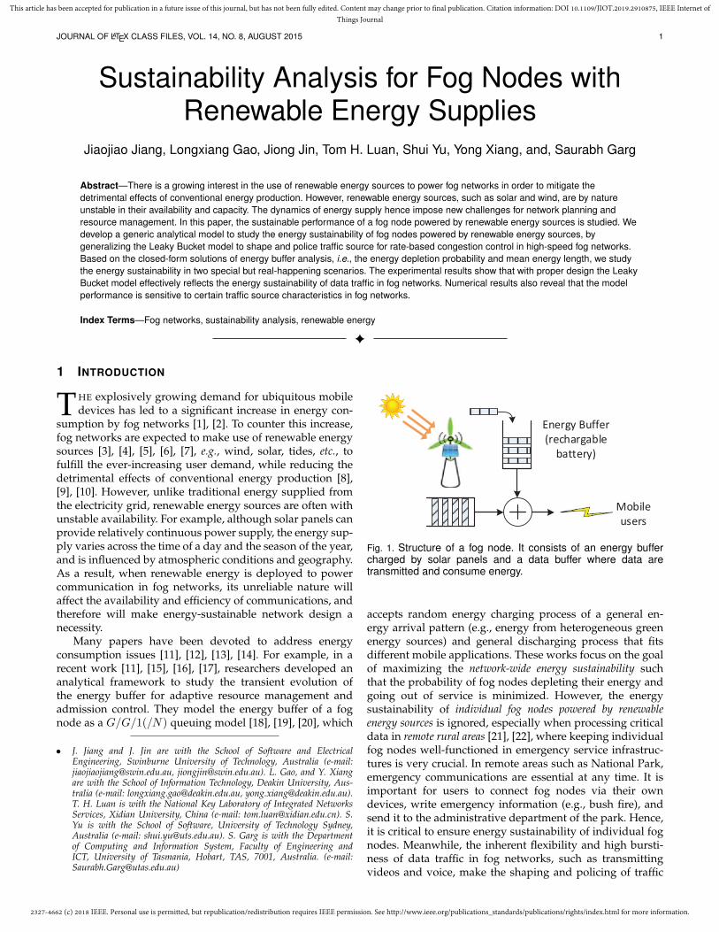
Fig. 1. Structure of a fog node. It consists of an energy buffercharged by solar panels and a data buffer where data aretransmitted and consume energy.

accepts random energy charging process of a general en-ergy arrival pattern (e.g., energy from heterogeneous greenenergy sources) and general discharging process that fitsdifferent mobile applications. These works focus on the goalof maximizing the network-wide energy sustainability suchthat the probability of fog nodes depleting their energy andgoing out of service is minimized. However, the energysustainability of individual fog nodes powered by renewableenergy sources is ignored, especially when processing criticaldata in remote rural areas [21], [22], where keeping individualfog nodes well-functioned in emergency service infrastruc-tures is very crucial. In remote areas such as National Park,emergency communications are essential at any time. It isimportant for users to connect fog nodes via their owndevices, write emergency information (e.g., bush fire), andsend it to the administrative department of the park. Hence,it is critical to ensure energy sustainability of individual fognodes. Meanwhile, the inherent flexibility and high bursti-ness of data traffic in fog networks, such as transmittingvideos and voice, make the shaping and policing of traffic




control problems of such networks very critical and makethe energy resource management at individual nodes verycrucial.

In this paper, we focus on the energy sustainabilityof fog nodes with renewable energy supplies in fog net-works, especially in the remote rural areas. Fig. 1 showsthe structure of a fog node charged by solar panels. It ismainly composed of an energy buffer and a data buffer.The energy buffer has variable energy arrival rates due tothe unstable availability of renewable energy sources. Withadequate energy storage, data traffic in the data buffer couldbe transmitted and consume energy. We first generalize theLeaky Bucket stochastic fluid model [23] to shape and policebursty data traffic in fog networks. In our generalized LeakyBucket model, we model the incoming data traffic as an N-state Markov modulated fluid sources. The energy arrivalrate r reflects different stages of energy supply scenarios.The Leaky Bucket corresponds to a counter, which is in-cremented each time a cell is generated by the source andis decremented periodically with a suitable leaky rate. TheLeaky Bucket can be analyzed as a G/D/1/N queue withfinite waiting room N and a suitable arrival process. Eachactive virtual connection has its own counter. Fig. 2 portraysthe Leaky Bucket model on a fog node.

Based on the Leaky Bucket model, we then develop amathematical model to analyze the “energy sustainability”performance of fog nodes theoretically under certain en-ergy sustainability constraints. More specifically, we firstderive the the closed-form distributions of data buffer andand energy buffer in the stochastic fluid model. Then, wecompute the mean lengths of data buffer and energy buffer.According to the mean energy buffer length, we considertwo particular but real-happening scenarios of energy sus-tainability. Again, we use the renewable energy source, solar(see Fig. 1), as an example to introduce the two scenarios.Solar panels can generate relatively stable power energyduring sunny daylights, but it cannot generate energy atnight. In order to supply ordinary data transmission atnight, it is necessary to consider (1) how much data unitsthe remaining energy can supply for ordinary data trans-mission. Another example would be in raining days, it isreasonable to assume there is no energy supply by solarpanel. If the rain last for a few days (in raining season), weneed to consider (2) how much remaining energy buffer isrequired to support a certain days of emergency data trans-mission. We mathematically analyze energy sustainabilityrelated to these two fundamental questions, and finallynumerically verify the proposed model can properly reflectsenergy sustainability of fog nodes.

We summarize the key contributions in this paper asfollows.

• We model the high diversity and burstiness of datatraffic and energy consumption in fog networks byextending the Leaky Bucket model.

• We derive the the closed-form distributions of databuffer and and energy buffer, and the mean lengthsof data buffer and energy buffer.

• According to the Leaky Bucket model, two funda-mental questions related to energy sustainability aremathematically analyzed and numerically verified.

Markov-modulated

fluid traffic

Data buffer

BD

BE Energy buffer

Energy arrival rate r

Departing cells

X

Y

Fig. 2. Leaky Bucket stochastic fluid model. The data traffic ismodeled as an N-state Markov modulated fluid sources, and theenergy supply is modeled with a stage-based constant energyarrival rate.

The rest of this paper is organized as follows. The analy-sis of the Leaky Bucket model is presented in Section 2. Wecarry out the analysis of energy sustainability performancein Section 3. Section 4 applies the analysis based on thedeveloped Leaky Bucket model on a simple but illustrativeexample: the ON-OFF data source scenario. Experimentalresults of the model performance are presented in Section 5.Section 6 concludes the remarks of this paper.

TABLE 1Notations used in paper.

Notation Description

µij The transition rate from state i to state j in the N -state

Markov-modulated Poisson process of data flow.

λi The state-dependent rate at state i in the Poisson process.

πi The stationary state probability for state i.

BD Data bucket capacity in the Leaky Bucket model.

BE Energy bucket capacity in the Leaky Bucket model.

Xt The contents of data buffer at time t.

Yt The contents of energy buffer at time t.

α The transition rate from OFF state to ON state.

β The transition rate from ON state to OFF state.

2 MODELING ENERGY BUFFERING AND DATABUFFERING

In this section, we first introduce a stage-based model forenergy buffering. Then, we generalize the Leaky Bucketmechanism to model data traffic shaping and policing ata fog node. The main notations used in this paper are listedin Table 1.

2.1 Stage-based Model of Energy BufferingWith the increasing number of applications moving on tofog networks, using renewable energy to power edge nodeshas become a significant strategy to alleviate the increasing




Hour

Po

we

r (M

W)

18 20 22 24

0

150

300

450

600

750

19 21 23

Fig. 3. A typical wind power curve of E.ON Netz in 3rd November2002 [24].

En

erg

y

bu

ffe

r

Time

Fig. 4. An illustration of energy buffer at different time stages. It isassumed that the energy power supply keeps consistent withineach time stage.

energy demands. In particular, as edge infrastructures aresmaller in size than centralized data center, they can make abetter use of renewable energy. However, renewable energysource (such as wind power and solar power) is often influ-enced by atmospheric conditions and geography, so it oftenpresents a fluctuating energy generation process. Figure 3shows a typical wind power curve of the E.ON Netz area[24] at 3rd November 2002. As we can see it presents a fluc-tuating process, and it is difficult to mathematically modelthe dynamic and real-time renewable energy generatingprocess.

In this paper, we simplify the renewable energy gener-ating process by assuming that renewable energy supply keepsconstant at each certain stage of an hour (or day or week).For example, in Figure 3, it is reasonable to assume thatthe wind power is relatively in each hour. Another examplewould be solar energy power. We may split a day intothree time stages (7am–10am, 10am–5pm, and 5pm–7am),and solar power output is relatively consistent at each timestage. Fig. 4 illustrates the energy arrival rate differing fromstage to stage, but within each stage the energy arrival rateis consistent.

2.2 Leaky Bucket Model of Data BufferingIn this subsection, we generalize the Leaky Bucket mech-anism to model data traffic shaping and policing on afog node. The “Leaky Bucket algorithm” [25], [26], andits performance have been analyzed in many works, suchas [27], [28], [29]. Fig. 2 portrays the Leaky Bucket modelon a fog node. In general, the Leaky Bucket algorithm ischaracterized by its bucket depth or threshold (BD) and itsleak rate (BE) as shown in Fig. 2. The basic idea is that acertain amount of fluid is added to the bucket contents eachtime a cell enters the network. The bucket leaks at a constant

rate set equal to the cell rate as agreed for that particularconnection. If cells are sent at a higher rate than the leakrate, the level of the fluid inside the bucket will rise until acertain critical level (the bucket limit) is exceeded. Then it isconcluded that the connection violates the agreed rate andthe cell is discarded. For discarded cells no fluid is added.All cells for that connection will be blocked until the bucketlevel has dropped below the limit. Hence, Leaky Bucketalgorithm has been commonly used in monitoring peakand average traffic rates of variable bitrate (VBR) services.Through setting the average traffic rates according to theLeaky Bucket algorithm and thereafter we can control traffic.From Fig. 2, we see that there are three critical parametersinvolved in Leaky Bucket algorithm: energy arrival rater, energy buffer capacity BE , and data buffer capacityBD. Additionally, in the Leaky Bucket model, batteries arerequired for storing the renewable energy and dischargingpower in data transmission. Hence, we assume the batteriesare with appropriate capacities and a certain number ofcycles of useful life. In the following, we will analyze theprobabilities of energy buffer and data buffer.

Now, we carry out a general analysis of Leaky Bucketalgorithm from which the energy sustainability can be read-ily derived. Fig. 2 portrays a fluid analysis version of thedata traffic. The energy arrival rate and the energy bucketsize are r and BE respectively, and the data buffer size isBD. The incoming bursty data traffic is modeled as an N -state Markov-modulated Poisson process (MMPP) (see Fig.5). Transition from state i to state j is governed by a Markovchain with a rate parameter µij for 1 ≤ i, j ≤ N , and theinput rate of the fluid data at state i is λi. The underlyingcontinuous time Markov chain of the fluid data for its statetransition can be represented by an N × N infinitesimalgenerating matrix M , defined by

M =

µ11 µ12 · · · µ1j · · · µ1N

µ21 µ22 · · · µ2j · · · µ2N

......

......

µi1 µi2 · · · µij · · · µiN...

......

...µN1 µN2 · · · µNj · · · µNN

, (1)

where, the diagonal rate parameter µii is given as

µii = −N∑

j=1,j 6=iµij , 1 ≤ i ≤ N. (2)

Then, the steady-state probability πi that the Markov chainis in state i can then be derived by solving the followingequation

πM = 0, (3)

where, the row vector π is of theN steady state probabilities

π =[π1 π2 · · · πi · · · πN

],

and a normalization condition∑Ni=1 πi = 1.

Assume two random variables Xt and Yt are the con-tents of the data buffer and the energy buffer at time t,where 0 ≤ Xt ≤ BD and 0 ≤ Yt ≤ BE . The objectiveis now to find the steady-state occupancy statistics of thetwo buffers, Xt and Yt, for the data and energy buffers,




1 2 3 i N

λ1 λ2 λ3 λi λN

µ21 µ32

µ1N

µ12 µ2i µiN

State-dependent

fluid input rates

Fig. 5. Markov-modulated fluid data model.

respectively. As soon as the buffer occupancy statistics ofXt and Yt are known, the cell loss and other performancemetrics can be found. In practice, however, the statisticsof Xt and Yt cannot be found separately since these tworandom variables are highly related to each other. Instead,we apply the method in [30], and define an equivalent“virtual” queue representation of Xt and Yt jointly. Notethe following two facts from the Leaky Bucket technique:

1) The data buffer can be occupied only if the energyqueue is empty (Yt = 0); otherwise the data cellswould be transmitted, one per energy buffer (Xt ≥0). Hence,

Yt = 0, Xt ≥ 0. (4)

2) Conversely, the energy buffer can be occupied onlyif the data buffer is empty (Xt = 0). If data cellswere queued, they would each capture a unit ofenergy and be transmitted (Yt ≥ 0). Hence,

Xt = 0, Yt ≥ 0. (5)

The equality (Yt = 0, Xt = 0) in Eq. (4) and Eq. (5) holdsfor the initial state where data buffer and energy buffer areempty. Now, combining Eqs. (4) and (5), we obtain

XtYt = 0. (6)

Therefore, instead of finding the individual statistics of Xt

or Yt directly, we shall find the joint probability first fromwhich the data cell loss is then derived.

Following the approach of [30], by combining the twobuffers of Xt and Yt together, we now define the followingsingle “virtual buffer” random variable Wt

Wt ≡ Xt − Yt +BE . (7)

Given the ranges of Xt and Yt and the condition in Eqs.(4) and (5), by defining B as the sum of the two buffer sizes,

B ≡ BD +BE . (8)

We note that Wt has the following properties:

1) 0 ≤Wt ≤ B.2) In the range 0 ≤Wt ≤ BE ,

Xt = 0, Wt = BE − Yt. (9)

3) In the range BE ≤Wt ≤ B = BE +BD,

Yt = 0, Wt = Xt +BE . (10)

BE

W

Y = 0

0 B=BE + BD

0BE

BDX = 0 X

Y

Fig. 6. “Virtual buffer” variable Wt.

Once the statistics of Wt is found, we can find the statisticsof Xt and Yt using the second and the third property above.The range of Wt and its relation to Yt are diagrammed inFig. 6. Define the joint probability of w,

Fi(w) = Pr [Wt ≤ w, S = i] , (11)

at time t at state i of the input data Markov chain, 1 ≤ i ≤N . Note from the definition of Wt that this implies

Fi(B) = πi. (12)

We derive the solution to Fi(w) based on the approach in[31]. The solution to Fi(w) is given by the solutions to thefollowing set of differential equations,

(λi − r)Fi(w)

dw=

N∑j=1

µjiFj(w), 1 ≤ i ≤ N. (13)

It is straightforward to obtain the governing differentialequations:

dF (w)

dwD = F (w)M, (14)

where

F (w) =[F1(w) F2(w) · · · FN (w)

],

M is the matrix of Eq. (1), and D is N ×N diagonal matrix

D ≡ Diag [λi − r] . (15)

Let scalar F (w) be the sum of state probability Fi(w),

F (w) =N∑i=1

Fi(w). (16)

Combining Eqs. (14) and (16) and the analysis in [32], weobtain the solution to Eq. (14) as follows:

dF (w) =N∑j=1

ajΦjezjw, (17)

where, (zj ,Φj) is the (eigenvalue, eigenvector) pair satisfy-ing the eigenvalue equation

zjΦjD = ΦjM , 1 ≤ j ≤ N. (18)

The aj ’s, 1 ≤ j ≤ N , are constants to be determinedby invoking N boundary conditions. Since πM = 0, oneeigenvalue of Eq. (18) must be zero. Calling this eigenvaluez1, its associated eigenvector Φ1 = π. Hence, Eq. (17) canbe simplified to

F (w) = a1π +N∑j=2

ajΦjezjw. (19)




2.3 Distributions of Data Buffer and Energy Buffer

In this subsection, we will derive the closed-form distribu-tions of data and energy buffers based on the Leaky BucketModel. According to Eq. (19), we know that we need Nboundary conditions to find the unknown constants aj ,1 ≤ j ≤ N to get the explicit form of F (w). To establishthese, we note that some of the Markov chain states must beunderload or “downward” states for those states i, λi < r;the others must be overload or “upward” states for thoseStates i, λi > r. Hence, all N states of the Markov chainmodulating the data arrival rate can be divided into twodisjoint sets,

SU ≡ {i ∈ N |λi − r > 0} : upward states; (20)

and

SD ≡ {i ∈ N |λi − r < 0} : downward states. (21)

Consider an arbitrary downward state, i ∈ SD. Since,the data arrival rate is less than the energy arrival rate inthese states, λi < r, the energy is tending to collect. Thedata queue is tending to empty (Xt → 0) and the energyqueue is tending to fill (Yt → BE). Hence,

Wt = Xt − Yt +BE → 0 (22)

For these states then, the probability the “virtual queue” isfull tends to zero, or we can write

Pr[Wt = B,S = i] = 0, i ∈ SD (23)

As Eq. (23) is the PDF (Probability Density Function) ofW , we note that Pr[Wt = B,S = i] is equal to the dif-ference between the CDFs (Cumulative Distribution Func-tion) Pr[W ≤ B,S = i] − Pr[Wt ≤ B−, S = i], i.e.,Fi(B)−Fi(B−). Note that B− is our notation for the largestvalue less than B in the PDF of Wt. Given Eq. (12), we thushave

Fi(B−) = πi, i ∈ SD. (24)

Consider an arbitrary upward state, i ∈ SU . For thesestates, with λi > r, the energy buffer tends to empty (Yt →0), the data buffer tends to fill (Xt → BD), and

Wt = Xt − Yt +BE → BD +BE = B. (25)

For these states, then, the probability that the virtual queueis empty must be zero. We thus have

Fi(0+) = Pr[Wt ≤ 0+, S = i] = 0, i ∈ SU . (26)

Note that 0+ is our notation for the smallest value largerthan 0 in the PDF of Wt.

Since a state is either a downward state or upwardstate, Eqs. (24) and (26) provide the necessary N boundaryconditions from which to find the N unknown constants aj ,1 ≤ j ≤ N , of Eq. (19). The N equations to be solved forthe N unknown aj could be written out in scalar form asfollows:

1) i ∈ SD :

Fi(B−) = πi = a1πi +

N∑j=2

ajΦjiezjB

−. (27)

2) i ∈ SU :

Fi(0+) = 0 = a1πi +

N∑j=2

ajΦji. (28)

Having found the distributions of Wt, we now canextract from it the distributions of the energy buffer contentYt and the data buffer content Xt. Specifically, we obtain

Pr[data buffer full] = 1− F (B), (29)

Pr[energy buffer full] = F (0), (30)

and we also obtain

Pr[Xt ≤ x, S = i] = Fi(x+BE), 0 ≤ x ≤ BD, (31)

and

Pr[Yt ≤ y, S = i] = πi − Fi(BE − y), 0 ≤ y ≤ BE , (32)

where, Fi(·) and F (·) are defined in Eqs. (11) and (16),respectively.

So far, we have derived the closed-form distributions ofdata buffer and energy buffer in Eq. (31) and Eq. (32), respec-tively. Based on these two distributions, we will analyze theenergy sustainability in the next section.

3 ENERGY SUSTAINABILITY ANALYSIS

Based on the fluid-flow analysis of the Leaky Bucket model,we now study the energy sustainability in this section.

According to the above assumption, we now need toanalyze the energy sustainability of fog nodes at certainstage rather. For other stages, we just need to carry outthe same analysis on each stage. In the following, we par-ticularly analyze data transmission under some special butreal-happening situation—the fail of energy buffer supply. Letus consider the solar power energy as an example, wherethe energy buffer is generated by solar panel. The solarpanel can generate relatively stable power energy duringsunny daylights. However, it could not generate energy atnight. Hence, we need to consider (1) how much data unitsthe remaining energy can supply for ordinary data transmission.Particularly, in raining days, it is reasonable to assume thereis no energy supply by solar panel. If the rain last for a fewdays (in raining season), we need to consider (2) how muchremaining energy buffer is required for support a certain days ofemergency data transmission.

In the following sub-sections, we first analyze and deriveclosed-form distributions of the mean data buffer lengthand energy buffer length. Then we analyze the energysustainability under the above two scenarios.

3.1 Mean Data Length and Energy Length

From Eqs. (32) and (31), we can obtain the overall distribu-tions of data buffer and energy buffer [33], [34] as follows:

Pr[Xt ≤ x] =∑i

Fi(x+BE) = F (x+BE), (33)

and

Pr[Yt ≤ y] =∑i

(πi − Fi(BE − y)) = 1−F (BE−y). (34)




Particularly, we have

{Pr[Xt ≤ BD] = F (BD +BE) = F (B),Pr[Yt ≤ BE ] = 1− F (BE −BE) = 1− F (0).

(35)

According to Eq. (19), we obtain the following equationto calculate F (w) for an arbitrary w ∈ [0, B]:

F (w) =∑i

Fi(w) = a1 +N∑j=2

ajezjw ·

∑i

Φji (36)

Hence, we can rewrite Eqs. (34) and (33) as follows:

Pr[Yt ≤ y] = 1−

a1 +N∑j=2

ajezj(BE−y) ·

∑i

Φji

, (37)

and

Pr[Xt ≤ x] = a1 +N∑j=2

ajezj(x+BE) ·

∑i

Φji. (38)

We use E[Xt] to denote the mean data buffer, then E[Xt]can be calculated as follows:

E[Xt] =

∫ B−D

0xdPr[Xt ≤ x] +BD · Pr[Xt = BD]

=

∫ B−D

0xdPr[Xt ≤ x] +BD · (1− Pr[Xt < BD])

=

∫ B−D

0xdPr[Xt ≤ x] +BD · (1− F (BD +BE))

=

∫ B−D

0xd

a1 +N∑j=2

ajezj(x+BE) ·

∑i

Φji

+BD ·

1−

a1 +N∑j=2

ajezj(BD+BE) ·

∑i

Φji

= x

a1 +N∑j=2

ajezj(x+BE) ·

∑i

Φji

∣∣∣∣x=B−D

x=0

−∫ B−

D

0

a1 +N∑j=2

ajezj(x+BE) ·

∑i

Φji

dx+BD ·

1−

a1 +N∑j=2

ajezj(BD+BE) ·

∑i

Φji

= (1− a1)BD +

N∑j=2

ajzjezjBE ·

∑i

Φji · (1− ezjBD ).

(39)

Similarly, we useE[Yt] to denote the mean energy buffer,

then E[Yt] can be calculated as follows:

E[Yt] =

∫ B−E

0ydPr[Yt ≤ y] +BE · Pr[Yt = BE ]

=

∫ B−E

0ydPr[Yt ≤ y] +BE · (1− Pr[Yt < BE ])

=

∫ B−E

0ydPr[Yt ≤ y] +BE · F (0)

=

∫ B−E

0yd

1− a1 −N∑j=2

ajezj(BE−y) ·

∑i

Φji

+BE ·

a1 +N∑j=2

aj ·∑i

Φji

= y

1− a1 −N∑j=2

ajezj(BE−y) ·

∑i

Φji

∣∣∣∣y=B−E

y=0

−∫ B−

E

0

1− a1 −N∑j=2

ajezj(BE−y) ·

∑i

Φji

dy+BE ·

a1 +N∑j=2

aj ·∑i

Φji

= a1BE −

N∑j=2

ajzj·∑i

Φji · (1− ezjBE ).

(40)

3.2 Energy Sustainability

Now, suppose there is no energy supply after a certain time.That is to say, the energy arrival rate r becomes 0. Here,we analyze the energy sustainability of the two scenariosdescribed in the opening of Section 3: the maximum dataunits can be transmitted based on the remaining energybuffer, and the minimum energy buffer required to supporta certain period of emergency data transmission. Both of thescenarios requires us to know the upper bound of energybuffer units required for every unit of data transmission.The following analysis investigates the upper bound fromthe aspect of the average data throughput 〈λ〉.

The average throughput 〈λ〉 can be calculated in a num-ber of equivalent ways. One is to say that this is the averageload, other than the cell loss when the data buffer is full.This could be written as

〈λ〉 =N∑i=1

λiπi −N∑i=1

(λi − r)Pr[Xt = BD, S = i]. (41)

The first term on the right-hand side is the average load, av-eraged over allN states. The second term is the average datacell loss, also averaged over theN states. However, note thatthe upward states only will be included in the second sumin Eq. (41) since we have already seen that in the downwardstates the data buffer cannot be full and cells cannot be lost(see Eq. (23)). The probability Pr[Xt = BD, S = i] that thedata buffer is full with the system in overload state i, isreadily calculated as

Pr[Xt = BD, S = i]= Pr[Wt = B,S = i]= Pr[Wt ≤ B,S = i]− Pr[Wt ≤ B−, S = i]= πi − Fi(B−).

(42)




We thus have, from Eq. (41),

〈λ〉 =N∑i=1

λiπi −N∑i=1

(λi − r)[πi − Fi(B−)

]. (43)

This can be rewritten as follows,

〈λ〉 = r +N∑i=1

Fi(B−)(λi − r). (44)

Assuming that every unit of data buffer transmissionrequires e units energy buffer, then we have the followingin-equation

e ≤ BE〈λ〉

. (45)

If e > BE/ 〈λ〉, the arrival energy will aways insufficientfor data transmission, which will result into too much dataloss in transmission and little energy for sustainability. Inaddition, energy supply devices generally requires someenergy for the basic functionality. Here, we assume anenergy supply device needs at least ξ(ξ � BE) energystored for functionality.

Finally, we analyze energy sustainability for the twoaforementioned scenarios. For scenario (1), we need to ana-lyze how much data units the remaining energy can supplyfor ordinary data transmission. That is to say, the fluid datainput rates λi are the same as before the fail of energysupply. From Eqs. (39) and (40), we have obtained the meandata buffer left and mean remaining energy buffer. Then, themaximum data units xmax the remaining energy can supplyis

xmax =E[Yt]− ξ

e− E[Xt]. (46)

For scenario (2), we need to analyze, how much remain-ing energy buffer is required to support a certain time ofemergency data transmission. That is to say, the averagefluid data input rate λ′ is different from the average ordinarydata input rate λ, where λ � λ′. Suppose, over the certaintime period (e.g., a day/week/month), the total emergencydata is xtotal. It requires xtotal · e units of energy to transmitthe data. Hence, the minimum energy ymin required is

ymin = (xtotal + E[Xt]) · e+ ξ. (47)

Similarly, we can calculate the probability of transmittingxtotal units of data by adjusting the Leaky Bucket model.

4 EXAMPLE OF ON-OFF DATA SOURCES

In Section 2.2, we model the incoming bursty data trafficas an N-state Markov modulated fluid flow (see Fig. 5),where the transition from state i to state j is governed by a

1 2

RP

β

α

off

Fig. 7. Simple ON-OFF fluid data source.

Markov chain with a rate parameter µij for 1 ≤ i, j ≤ N .In this section, we apply the above proposed Leaky Bucketmodel and the analysis of energy sustainability on a simplebut illustrative 2-state Markov data model, the ON-OFF datasource model (see Fig. 7). In Fig. 7, the inter-arrival rates are 0and Rp in the OFF state and the ON state respectively. Thiscould be representative of a voice data source or an imagedata source, depending on the choice of parameters. Alsoassume the transition rate from OFF state to ON state is αand from ON state to OFF state is β. In this model, notethat the OFF state refers to state 1 and ON state refers tostate 2 in the analysis. Notice that λ1 = 0, λ1 = Rp, and thecontinuous time Markov chain generating matrix and thesteady state probability row vector are as follows

M =

[µ11 µ12

µ21 µ22

]=

[−α αβ −β

],

andπ =

[π1 π2

]=[

βα+β

αα+β

].

Here, there is only one eigenvalue z to be found.Through basic computation, we have

z = − α+ β

Rp − r(1− ρ), (48)

where

ρ =Rpr

(α

α+ β

)=Rpp

r, with p ≡ α

α+ β. (49)

For the single eigenvector Φ = [Φ1,Φ2] appearing in Eq.(28), we have

Φ1/Φ2 = (Rp − r)/r =

(Rpr− 1

). (50)

Letting Φ2 = 1 arbitrarily, we get, for this example,

F (x) = a1π + a2

[(Rpr− 1

), 1

]ezx. (51)

The two unknown constants a1 and a2 are found using theboundary conditions of Eqs. (27) and (28). In this simpleexample, withN = 2 states only, state one with λ1 = 0 is thedownward state and state two with λ2 = Rp is the upwardstate. We must thus have 0 < r < Rp for the fluid analysisto provide a stationary solution in this case. This impliesthat the single eigenvalue z of Eq. (48) will be negative ifthe parameter ρ defined by Eq. (49) is less than 1.

From Eq. (27), we have, using Eq. (51),

F1(B−) = π1 = a1π1 + a2

(Rpr− 1

)ezB

−, (52)

with π1 = (1− p) = β/(α+ β).Similarly, from Eqs. (28) and (51), we have

F1(0+) = 0 = a1π2 + a2, (53)

where π2 = p = α/(α+ β).Solving Eqs. (52) and (53) simultaneously for a1 and a2,

we get

a1 = 1/

[1− α

β

(Rpr− 1

)ezB

], (54)

anda2 = −π2a1 = −a1α/(α+ β). (55)




Using Eqs. (54) and (55) in Eq. (51), we finally get the twoprobability distribution functions in this case of a single ON-OFF data source,

F1(w) = π1∆(w)/∆(B), (56)

andF2(w) = π2(1− ezw)/∆(B), (57)

with

∆(w) ≡ 1− α

β

(Rpr− 1

)ezw, (58)

where π1 = β/(α+ β), π2 = 1− π1 = α/(α+ β), and z aregiven by Eq. (48). Then, we have

F (w) = F1(w) + F2(w) =1− ρezw

∆(B). (59)

All the performance analysis of interest can be obtainedfrom F (w). For example, for the average data throughput,recall that λ1 = 0, λ2 = Rp, ρ ≡ Rpp/r, p = α/(α + β) inON-OFF data sources. Then it is readily shown, using Eqs.(56) and (57) in (44), that the normalized throughput for thisexample is given by

〈λ〉 /r = 1− (1− ρ)/∆(B), (60)

where, ∆(B) is defined in Eq. (58).Similarly, the mean length of data buffer E[Xt] in the

ON-OFF data sources becomes:

E[Xt] =

∫ B−D

0xd[F (x+BE)] +BD · (1− F (B))

=

∫ B−D

0xd

1− ρez(x+BE)

∆(B)+BD · (1−

1− ρezB

∆(B))

= BD −∫ B−

D

0dx− ρ

z ez(x+BE)

∆(B)

= BD −BD − ρ

z ezB

∆(B)+−ρz e

zBE

∆(B)

=ρ(ezB − ezBE )

z∆(B)+BD(1− 1

∆(B)).

(61)The mean length of energy buffer E[Yt] in ON-OFF datasources becomes:

E[Yt] =

∫ B−E

0yd [1− F (BE − y)] +BE · F (0)

=

∫ B−E

0yd

[1− 1− ρez(BE−y)

∆(B)

]+BE ·

1− ρ∆(B)

= BE −∫ B−

E

0d

[y −

y + ρz ez(BE−y)

∆(B)

]=ρ(1− ezBE )

z∆(B)+

BE∆(B)

.

(62)

Then, for the two scenarios of energy sustainabilityanalysis in the ON-OFF data sources, we can get (1) themaximum data buffer xmax which could be transmittedwhen energy rate becomes 0, and (2) the minimum energybuffer ymin required for transmitting a certain amount ofemergency data transmission.

0 5 10 15 20

Energy buffer space (BE

)

0

5

10

15

20

Me

an

le

ng

th

ana (Energy)

ana (Data)

sim (Energy)

sim (Data)

Fig. 8. Mean data length and mean energy length as a functionof total buffer space B, with ρ = 0.81.

5 NUMERICAL RESULTS

In this section, we validate the energy buffer analysis andevaluate the energy sustainability performance through an-alytical results and simulation results. All the experimentsare implemented on MatLab. We particularly use the ON-OFF data source model for experiments. In the exact LeakyBucket model, the data source alternates between the ONstate and the OFF state. During the ON state, whose meanduration is 1/β seconds; the source transmits data cells(which are with fixed length packets) at a constant rate ofr cells per second. The energy arrives at the energy bucketat a constant rate of r energy buckets per second. To ensurethat the data traffic density is relatively moderate (whereα/β < 1) rather than extremely intensive (where α/β ≈ 1),we particularly set β and α to 1.0 and 0.57. We set Rp = 1and r is chosen from {0.45, 0.42, 0.39}. We set the maximumtotal buffer size B as 20 and let BE increase from 0 to 20.For each group of parameter values (in terms of B,BE andr), we get the average simulation result over 100 runs whereeach run consists of 100 attempts of data transmission.

We first investigate the mean data length and meanenergy length on energy arrival rate (r) and energy buffersize (BE). From Eqs. (61) and (40), we know that E[Xt]depends on z (which ultimately depends on r), and BE .The experimental results are shown in Figs. 8, 9, and 10,corresponding to r = {0.45, 0.42, 0.39}, respectively. Fromthese figures, we see that the the simulation results are veryclose to the analytical results across different parameter set-tings. When the energy arrival rate decreases, the simulationresults become conservative and thus slightly lower than theanalytical results. Overall, the mean energy buffer lengthincreases with the increase of energy buffer size BE , whilethe mean data buffer length decreases with the increase ofBE . Moreover, as energy traffic intensity ρ approaches 1 (oralternatively r close to the energy source mean rate), themean energy buffer length E[Yt] increases slower with BEand achieves a desirable as the size of BE . This is becausethe greater BE allows larger data transmission. Hence, theaverage length of energy becomes larger.




0 5 10 15 20


)

0

5

10

15

20

Mean length

ana (Energy)

ana (Data)

sim (Energy)

sim (Data)


0 5 10 15 20


)

0

5

10

15

20

Me

an

le

ng

th

ana (Energy)

ana (Data)

sim (Energy)

sim (Data)


We then investigate the energy sustainability of the twoparticular scenarios discussed in Section 3.2. The results aredisplayed in Fig. 11 and Fig. 12 for ρ = {0.81, 0.87, 0.93}against the energy buffer size BE . Fig. 11 presents themaximum units xmax of data could be transmitted after afailure of energy supply, and Fig. 12 presents the minimumunits ymin of energy buffer required to supply a certainunits of emergency data demergency transmission. Overall,the simulation results present to be relatively conservative.From the perspective of xmax, a smaller number of dataunits can be transmitted than analytical results when theenergy power supply fails. From the perspective of ymin, alarger number of energy units are required for emergencydata transmission when the energy power supply fails. InFig. 11, the energy buffer size BE ranges from 0 to 20 units.As energy buffer size BE increases, the maximum unitsxmax of data transmission also increases. In particular, thegreater ρ (or the less energy arrival rate r) the less data couldbe transmitted. This is because, the lower energy arrival

0 5 10 15 20


)

0

2

4

6

8

10

12

14

xm

ax

ana ( = 0.8081)

ana ( = 0.8658)

ana ( = 0.9324)

sim ( = 0.8081)

sim ( = 0.8658)

sim ( = 0.9324)

Fig. 11. The maximum units of data that the remaining energycould supply for ordinary data transmission.

0 5 10 15 20


)

2

4

6

8

10

12

14

ym

in

ana ( = 0.8081)

ana ( = 0.8658)

ana ( = 0.9324)

sim ( = 0.8081)

sim ( = 0.8658)

sim ( = 0.9324)

Fig. 12. The minimum units of energy required to support acertain period of emergency data transmission.

rate r the less energy can be stored, which in turn supportless data transmission after the failure of the energy powersupply. In Fig. 12, we particularly set demergency = 7. Aswe can see, ymin increases with BE . This is because, again,the lower energy arrival rate r the less energy can be stored,which in turn requires much more energy power (ymin) foremergency data transmission after the failure of the energypower supply.

6 CONCLUSION AND DISCUSSION

In this paper, we have generalized a stochastic fluid modelto analyze the energy sustainability performance on fognodes. We first generalize the well-known Leaky Bucketmodel to police and shape traffic from diverse and burstydata sources. Based on the Leaky Bucket model, we derivedclosed-forms for the distribution of energy buffer and databuffer, and the explicit formulas of mean energy buffer andmean data buffer, and achieved mathematically analysis ofthe energy sustainability performance on fog nodes. On the




basis of the Leaky Bucket model and the derived closed-form formulas, we perform numerical evaluations with theaim of assessing the effectiveness of the Leaky Bucket mech-anism and its effectiveness in reflecting the energy sustain-ability of of data traffic in fog networks. The experimentalresults have shown how the Leaky Bucket mechanism canbe used to police and shape traffic in emergency scenarios(e.g., the failure of energy supply). Numerical results havealso revealed the sensitivity of performance to source trafficassumptions.

Note that we assume that the energy arrival rate differsfrom stage to stage, but within each stage the energy arrivalrate is relatively consistent. In the real world, however, therenewable energy sources are often heterogeneous [35], andthe energy charging process is often stochastic and may followcertain distribution (e.g., time-varying Poisson distribution[36]). The Leaky Bucket model generalized in this paper isnot applicable for continues time-varying energy chargingprocess. As our future work, we plan to extend the LeakyBucket model for continues time-varying energy powersupply. Meanwhile, in this paper, the data buffer is assumedwith no MAC delay and the wireless links are assumed tobe reliable. However, real-world data transmission on fognetworks often involves MAC delay and unreliable wirelesslinks. Hence, our second future work is to extend currentmodel through considering those realistic network features.

REFERENCES

[1] M. Chiang and T. Zhang, “Fog and iot: An overview of researchopportunities,” IEEE Internet of Things Journal, vol. 3, no. 6, pp.854–864, 2016.

[2] I. Stojmenovic, S. Wen, X. Huang, and H. Luan, “An overview offog computing and its security issues,” Concurrency and Computa-tion: Practice and Experience, vol. 28, no. 10, pp. 2991–3005, 2016.

[3] L. Yu, T. Jiang, Y. Cao, and Q. Qi, “Carbon-aware energy costminimization for distributed internet data centers in smart mi-crogrids,” IEEE Internet of Things Journal, vol. 1, no. 3, pp. 255–264,2014.

[4] H. H. R. Sherazi, G. Piro, L. A. Grieco, and G. Boggia, “Whenrenewable energy meets lora: A feasibility analysis on cable-lessdeployments,” IEEE Internet of Things Journal, 2018.

[5] L. Lei, Y. Kuang, X. S. Shen, K. Yang, J. Qiao, and Z. Zhong, “Op-timal reliability in energy harvesting industrial wireless sensornetworks,” IEEE Transactions on Wireless Communications, vol. 15,no. 8, pp. 5399–5413, 2016.

[6] Q. Han, B. Yang, C. Chen, and X. Guan, “Energy-aware and qos-aware load balancing for hetnets powered by renewable energy,”Computer Networks, vol. 94, pp. 250–262, 2016.

[7] T. D. Hieu, B.-S. Kim et al., “Stability-aware geographic routingin energy harvesting wireless sensor networks,” Sensors, vol. 16,no. 5, p. 696, 2016.

[8] M. Moness and A. M. Moustafa, “A survey of cyber-physicaladvances and challenges of wind energy conversion systems:prospects for internet of energy,” IEEE Internet of Things Journal,vol. 3, no. 2, pp. 134–145, 2016.

[9] F. Bonomi, R. Milito, J. Zhu, and S. Addepalli, “Fog computing andits role in the internet of things,” in Proceedings of the first editionof the MCC workshop on Mobile cloud computing. ACM, 2012, pp.13–16.

[10] L. M. Vaquero and L. Rodero-Merino, “Finding your way in thefog: Towards a comprehensive definition of fog computing,” ACMSIGCOMM Computer Communication Review, vol. 44, no. 5, pp. 27–32, 2014.

[11] L. X. Cai, Y. Liu, T. H. Luan, X. Shen, J. W. Mark, and H. V. Poor,“Sustainability analysis and resource management for wirelessmesh networks with renewable energy supplies,” IEEE Journal onSelected Areas in Communications, vol. 32, no. 2, pp. 345–355, 2014.

[12] R. Deng, R. Lu, C. Lai, T. H. Luan, and H. Liang, “Optimal work-load allocation in fog-cloud computing toward balanced delay andpower consumption,” IEEE Internet of Things Journal, vol. 3, no. 6,pp. 1171–1181, 2016.

[13] W. Shi, J. Cao, Q. Zhang, Y. Li, and L. Xu, “Edge computing: Visionand challenges,” IEEE Internet of Things Journal, vol. 3, no. 5, pp.637–646, 2016.

[14] L. Gao, T. H. Luan, S. Yu, W. Zhou, and B. Liu, “Fogroute: Dtn-based data dissemination model in fog computing,” IEEE Internetof Things Journal, vol. 4, no. 1, pp. 225–235, 2017.

[15] R. Ranjan, O. Rana, S. Nepal, M. Yousif, P. James, Z. Wen, S. Barr,P. Watson, P. P. Jayaraman, D. Georgakopoulos et al., “The nextgrand challenges: Integrating the internet of things and datascience,” IEEE Cloud Computing, vol. 5, no. 3, pp. 12–26, 2018.

[16] A. Khoshkbarforoushha, R. Ranjan, R. Gaire, E. Abbasnejad,L. Wang, and A. Y. Zomaya, “Distribution based workload mod-elling of continuous queries in clouds,” IEEE Transactions onEmerging Topics in Computing, vol. 5, no. 1, pp. 120–133, 2017.

[17] D. Puthal, S. Nepal, R. Ranjan, and J. Chen, “A dynamic key lengthbased approach for real-time security verification of big sensingdata stream,” in International conference on web information systemsengineering. Springer, 2015, pp. 93–108.

[18] J. Kingman, “The single server queue in heavy traffic,” in Math-ematical Proceedings of the Cambridge Philosophical Society, vol. 57,no. 4. Cambridge University Press, 1961, pp. 902–904.

[19] W. Fischer and K. Meier-Hellstern, “The markov-modulated pois-son process (mmpp) cookbook,” Performance evaluation, vol. 18,no. 2, pp. 149–171, 1993.

[20] T. Naishuo, “Queue m/g/1 with adaptive multistage vacation [j],”Mathematica Applicata, vol. 4, p. 002, 1992.

[21] J. Li, T. Zhang, J. Jin, Y. Yang, D. Yuan, and L. Gao, “Latencyestimation for fog-based internet of things,” in TelecommunicationNetworks and Applications Conference (ITNAC), 2017 27th Interna-tional. IEEE, 2017, pp. 1–6.

[22] T. Khatib, A. Mohamed, and K. Sopian, “A review of photovoltaicsystems size optimization techniques,” Renewable and SustainableEnergy Reviews, vol. 22, pp. 454–465, 2013.

[23] M. P. McGarry, M. Maier, and M. Reisslein, “Ethernet pons: asurvey of dynamic bandwidth allocation (dba) algorithms,” IEEEcommunications magazine, vol. 42, no. 8, pp. S8–15, 2004.

[24] B. Ernst, K. Rohrig, and R. Jursa, “Online-monitoring and pre-diction of wind power in german transmission system operationcentres,” in Proceedings of the First IEA Joint Action Symposium onWind Forecasting Techniques, Norrkoping, Sweden, 2002, pp. 125–145.

[25] M. Schwartz, Broadband integrated networks. Prentice Hall PTRNew Jersey, 1996, vol. 19.

[26] G. Niestegge, “The leaky bucketpolicing method in the atm (asyn-chronous transfer mode) network,” International Journal of Digital& Analog Communication Systems, vol. 3, no. 2, pp. 187–197, 1990.

[27] N. Yamanaka, Y. Sato, and K.-I. Sato, “Performance limitation ofleaky bucket algorithm for usage parameter control and band-width allocation methods,” IEICE Transactions on Communications,vol. 75, no. 2, pp. 82–86, 1992.

[28] N. Yin and M. G. Hluchyj, “Analysis of the leaky bucket algorithmfor on-off data sources,” Journal of High Speed Networks, vol. 2, no. 1,pp. 81–98, 1993.

[29] K. Sohraby and M. Sidi, “On the performance of bursty and mod-ulated sources subject to leaky bucket rate-based access controlschemes,” IEEE Transactions on Communications, vol. 42, no. 234,pp. 477–487, 1994.

[30] A. I. Elwalid and D. Mitra, “Stochastic fluid models in the analysisof access regulation in high speed networks,” in Global Telecommu-nications Conference, 1991. GLOBECOM’91.’Countdown to the NewMillennium. Featuring a Mini-Theme on: Personal CommunicationsServices. IEEE, 1991, pp. 1626–1632.

[31] D. Anick, D. Mitra, and M. M. Sondhi, “Stochastic theory of a data-handling system with multiple sources,” Bell Labs Technical Journal,vol. 61, no. 8, pp. 1871–1894, 1982.

[32] B. Noble, J. W. Daniel et al., Applied linear algebra. Prentice-HallNew Jersey, 1988, vol. 3.

[33] B. Everitt and A. Skrondal, The Cambridge dictionary of statistics.Cambridge University Press Cambridge, 2002, vol. 106.

[34] G. F. Reed, F. Lynn, and B. D. Meade, “Use of coefficient ofvariation in assessing variability of quantitative assays,” Clinicaland diagnostic laboratory immunology, vol. 9, no. 6, pp. 1235–1239,2002.




[35] R. Mahmud, R. Kotagiri, and R. Buyya, “Fog computing: Ataxonomy, survey and future directions,” in Internet of everything.Springer, 2018, pp. 103–130.

[36] A. Ihler, J. Hutchins, and P. Smyth, “Adaptive event detectionwith time-varying poisson processes,” in Proceedings of the 12thACM SIGKDD international conference on Knowledge discovery anddata mining. ACM, 2006, pp. 207–216.

Jiaojiao Jiang received the Ph.D. degree inSchool of Information Technology from DeakinUniversity, Australia in 2017. She is currently aPostdoctoral Research Fellow in the School ofSoftware and Electrical Engineering, SwinburneUniversity of Technology, Australia. Her researchinterests include service virtualization, cyber se-curity, and complex networks. She has servedas Program Chair, TPC Chair, Symposium Chair,and Session Chair for a number of internationalconferences, including GlobeCom and ICC.

Longxiang Gao received his PhD in ComputerScience from Deakin University, Australia. Heis currently a Lecturer at School of Informa-tion Technology, Deakin University. Before joinedDeakin University, he was a post-doctoral re-search fellow at IBM Research & DevelopmentAustralia. His research interests include dataprocessing, mobile social networks, Fog com-puting and network security. Dr. Gao has over 40publications, including patent, monograph, bookchapter, journal and conference papers. Some

of his publications have been published in the top venue, such as IEEETMC, IEEE IoT, IEEE TDSC and IEEE TVT. Dr. Gao is a Senior Memberof IEEE and active in IEEE Communication Society. He has served asthe TPC co-chair, publicity co-chair, organization chair and TPC memberfor many international conferences.

Jiong Jin received the B.E. degree with FirstClass Honours in Computer Engineering fromNanyang Technological University, Singapore, in2006, and the Ph.D. degree in Electrical andElectronic Engineering from the University ofMelbourne, Australia, in 2011. He is currently aSenior Lecturer in the School of Software andElectrical Engineering, Faculty of Science, En-gineering and Technology, Swinburne Universityof Technology, Melbourne, Australia. Prior to it,he was a Research Fellow in the Department

of Electrical and Electronic Engineering at the University of Melbournefrom 2011 to 2013. His research interests include network design andoptimization, fog and edge computing, robotics and automation, Internetof Things and cyber-physical systems as well as their applications insmart manufacturing and smart cities.

Tom H. Luan received his B.Eng. degree fromXi’an Jiao Tong University, China, in 2004, theM.Phil. degree from Hong Kong University ofScience and Technology in 2007, and Ph.D. de-gree from the University of Waterloo, Ontario,Canada, in 2012. He is a professor at the Schoolof Cyber Engineering of Xidian University, Xi’an,China. His research mainly focuses on contentdistribution and media streaming in vehicular adhoc networks and peer-to-peer networking, aswell as the protocol design and performance

evaluation of wireless cloud computing and edge computing. Dr. Luanhas authored/coauthored more than 40 journal papers and 30 technicalpapers in conference proceedings, and awarded one US patent. Heserved as a TPC member for IEEE Globecom, ICC, PIMRC and thetechnical reviewer for multiple IEEE Transactions including TMC, TPDS,TVT, TWC and ITS.

Shui Yu is currently a full Professor of Schoolof Software, University of Technology Sydney,Australia. Dr Yus research interest includes Se-curity and Privacy, Networking, Big Data, andMathematical Modelling. He has published twomonographs and edited two books, more than200 technical papers, including top journals andtop conferences, such as IEEE TPDS, TC, TIFS,TMC, TKDE, TETC, ToN, and INFOCOM. Dr Yuinitiated the research field of networking for bigdata in 2013. His h-index is 32. Dr Yu actively

serves his research communities in various roles. He is currently servingthe editorial boards of IEEE Communications Surveys and Tutorials,IEEE Communications Magazine, IEEE Internet of Things Journal, IEEECommunications Letters, IEEE Access, and IEEE Transactions on Com-putational Social Systems.

Yong Xiang received the Ph.D. degree in Elec-trical and Electronic Engineering from The Uni-versity of Melbourne, Australia. He is a Professorand the Director of the Artificial Intelligence andImage Processing Research Cluster, School ofInformation Technology, Deakin University, Aus-tralia. His research interests include informationsecurity and privacy, signal and image process-ing, data analytics and machine intelligence, andInternet of Things. He has published 2 mono-graphs, over 100 refereed journal articles, and

numerous conference papers in these areas. He is an Associate Editorof IEEE Signal Processing Letters and IEEE Access. He has served asProgram Chair, TPC Chair, Symposium Chair, and Session Chair for anumber of international conferences.

Saurabh Garg is currently a Lecturer with theUniversity of Tasmania, Australia. He is one ofthe few Ph.D. students who completed in lessthan three years from the University of Mel-bourne. He has authored over 40 papers inhighly cited journals and conferences. Duringhis Ph.D., he has been received various specialscholarships for his Ph.D. candidature. His re-search interests include resource management,scheduling, utility and grid computing, Cloudcomputing, green computing, wireless networks,

and ad hoc networks.

Sustainability Analysis for Fog Nodes with Renewable ...

Documents