Susskind Lectures on String Theory

Susskind Lectures on String Theory

July 10, 2022

version 2.1

These notes are from a series of lectures given by Leonard Susskind (one of thefounders of string theory). They follow the logic he used when he first started thinkingabout strings and are an exceptionally clear and accessible introduction to stringtheory. Susskind gave this series of lectures for retired engineers and other scientistsin his continuing education course at Stanford.1 I wrote these notes for graduatestudents interested in quantum gravity. These notes are not verbatim; I watched thelectures (while jogging) and reproduced them afterwards.

Part I of this document follows the lecture series by Susskind titled “String theoryand M-theory.” This is a basic introduction to bosonic string theory using the infi-nite momentum frame description. In this “light cone” frame one is able to quantizethe non-relativistic degrees of freedom in the transverse plane using canonical quan-tization. The massless excitations are examined and found to contain photon-likeand graviton-like particles, as well as tachyon states. We show that to obtain a zeromass for the photon-like state requires that the critical dimension of spacetime beD=26. The Veneziano amplitude is introduced in the context of meson scattering,and is, remarkably, shown to result from the scattering amplitude of two open bosonicstrings. Part II follows the Susskind lectures titled “Topics in String Theory”. PartII is incomplete.

If you find any errors or typos in this document please email them to me [email protected]. I hope you enjoy the notes.

1All of Susskind’s continuing education lectures are easily found on YouTube. Even for advancedstudents these lectures are well worth watching.

1

CONTENTS CONTENTS

Contents

Contents 2

List of Figures 3

I Bosonic String Theory 5

1 Particle Energies 51.1 Non-relativistic particles . . . . . . . . . . . . . . . . . . . . . . . . . 51.2 Composite particles . . . . . . . . . . . . . . . . . . . . . . . . . . . . 51.3 The infinite momentum frame . . . . . . . . . . . . . . . . . . . . . . 6

2 Infinite Momentum Frame 82.1 The continuum limit . . . . . . . . . . . . . . . . . . . . . . . . . . . 8

2.1.1 Canonical quantization of the string . . . . . . . . . . . . . . 82.1.2 Helicity for massless particles . . . . . . . . . . . . . . . . . . 112.1.3 Low energy excitations of the string . . . . . . . . . . . . . . 122.1.4 Open vs. closed strings . . . . . . . . . . . . . . . . . . . . . . 13

2.2 Closed string spectrum . . . . . . . . . . . . . . . . . . . . . . . . . . 132.3 Critical dimension . . . . . . . . . . . . . . . . . . . . . . . . . . . . 16

3 Open String Scattering 183.1 Mandelstam variables . . . . . . . . . . . . . . . . . . . . . . . . . . . 183.2 The Veneziano amplitude . . . . . . . . . . . . . . . . . . . . . . . . 213.3 Bosonic open string scattering . . . . . . . . . . . . . . . . . . . . . . 21

3.3.1 Euler Beta function . . . . . . . . . . . . . . . . . . . . . . . 25

4 World sheet symmetries 264.1 Conformal mapping . . . . . . . . . . . . . . . . . . . . . . . . . . . . 274.2 Compactification . . . . . . . . . . . . . . . . . . . . . . . . . . . . . 314.3 Winding number . . . . . . . . . . . . . . . . . . . . . . . . . . . . . 33

5 Kaluza-Klein 355.1 Kaluza-Klein metric . . . . . . . . . . . . . . . . . . . . . . . . . . . 355.2 D-branes . . . . . . . . . . . . . . . . . . . . . . . . . . . . . . . . . . 37

2

LIST OF FIGURES LIST OF FIGURES

II Topics in String Theory 38

6 Fundamental Objects 386.1 The electron and the monopole . . . . . . . . . . . . . . . . . . . . . 396.2 D-branes and S-duality . . . . . . . . . . . . . . . . . . . . . . . . . . 39

7 The Schwarzchild metric 417.1 Black holes . . . . . . . . . . . . . . . . . . . . . . . . . . . . . . . . 42

7.1.1 Information and entropy . . . . . . . . . . . . . . . . . . . . . 427.1.2 Black hole quantum mechanics . . . . . . . . . . . . . . . . . 437.1.3 Hidden degrees of freedom . . . . . . . . . . . . . . . . . . . . 45

7.2 Metric near the horizon . . . . . . . . . . . . . . . . . . . . . . . . . 467.2.1 Rindler space . . . . . . . . . . . . . . . . . . . . . . . . . . . 48

7.3 Penrose diagrams . . . . . . . . . . . . . . . . . . . . . . . . . . . . . 487.4 Black hole formation . . . . . . . . . . . . . . . . . . . . . . . . . . . 487.5 Counting black hole microstates . . . . . . . . . . . . . . . . . . . . . 49

List of Figures

1 Four-particle interaction with incoming momenta k1, k2 and outgoingmomenta q3, q4. . . . . . . . . . . . . . . . . . . . . . . . . . . . . . . 19

2 Feynman diagrams for S- (left) and t-channel (right) scattering withtime running from left to right. Making particle 4 incoming and 2outgoing corresponds to u-channel scattering. (The gluon line hererepresents many kinds of particles of different mass.) . . . . . . . . . 20

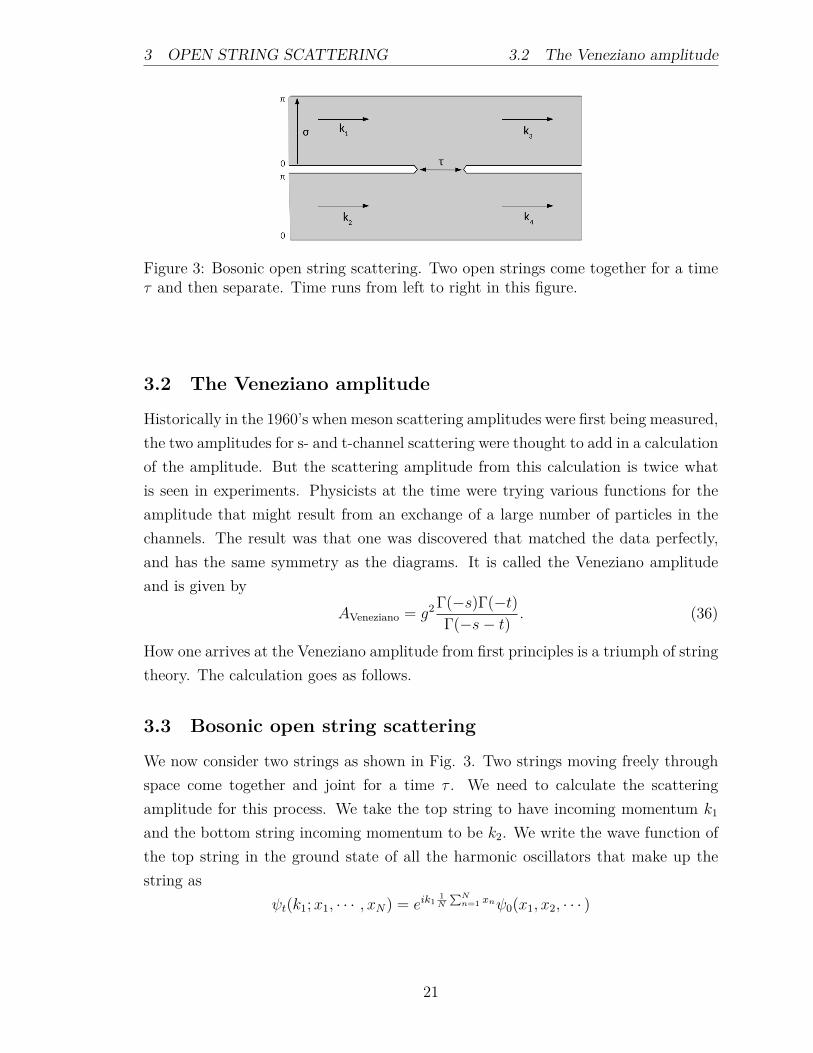
3 Bosonic open string scattering. Two open strings come together for atime τ and then separate. Time runs from left to right in this figure. 21

4 Conformal mapping of the two-string interaction in Fig. 3 to the unitdisk. The interior of the disk is the interior of the shaded string regionin Fig. 3 and the injection points are shown as exaggerated cutouts inthe disk. These are mapped to infinitesimal points on the exterior ofthe disk. . . . . . . . . . . . . . . . . . . . . . . . . . . . . . . . . . . 27

5 s- and t-channel scattering maps. The τ parameter determines thesymmetric locations of the four vertex operators. For τ = 0 the pointswould move closer and overlap on the left. For τ → ∞ the point onthe right map would move closer and overlap. . . . . . . . . . . . . . 27

3

LIST OF FIGURES LIST OF FIGURES

6 Linear fractional map w(z) = z+1z−1

. . . . . . . . . . . . . . . . . . . . . 297 Rindler spacetime diagram. The horizon of a black hole is the 45-

degree line defining the light cone from the origin. . . . . . . . . . . 488 Rindler metric, near and far from the horizon. . . . . . . . . . . . . . 48

4

1 PARTICLE ENERGIES

Part I

Bosonic String Theory

1 Energy of Non-relativistic and Relativistic Par-ticles

1.1 Non-relativistic particles

The energy of a “particle” is given the by the momentum of the particle plus therest mass of the particle plus whatever binding energy holds together the constituentparts. Classically, we write this as

E =p2

2m+mc2 +B. (1)

Here B represents the internal binding energy of the particle. If the particle remainsslow and is bound tightly, then this energy will never be observed and can be movedto the LHS of (1) with a redefinition of the energy E ′ = E −mc2 −B giving

E ′ =p2

2m. (2)

For example, the energy of a cup of coffee would be the momentum of the centerof mass of the motion of the coffee plus the rest mass m of all the atoms in the coffeeplus the binding energy B of the water in the coffee. The rest mass m of the coffeewould include the internal motion of the atoms (heat). The binding energy of thecoffee would be the latent heat needed to evaporate all of the coffee and this wouldgo into B.

1.2 Composite particles

What separates “elementary” particles from composite particles? It is the relativemagnitude of the energy required to increase the internal angular momentum of theinternal constituents of the particle.2 If this number is a large fraction of the rest mass

2In particle accelerator experiments a plot of mass squared m2 vs angular momentum J of pions,for example, shows a linear relationship. All hadrons including for example the pions (two-quarkparticles) and deltas (three-quark particles with spin 3/2) show the same behavior with the samesloping trajectories.

5

1.3 The infinite momentum frame 1 PARTICLE ENERGIES

of the particle it is considered to be an elementary particle. If the required energy is avery small fraction of the rest mass of the particle it is considered a composite particle.Examples here are given by the electron, an elementary particle, and the cup of coffee,which is clearly composite. An electron has spin ±h/2. Is it possible to “spin up”an electron to a higher angular momentum state similar to the way hadrons can bespun up, resulting in the Regge trajectories seen in particle accelerators? Classicallythe energy of a rotating object is given by the kinetic energy E = Iω2/2 and theangular momentum is given by L = Iω. Quantum mechanics dictates that angularmomentum is quantized in units of h. For a large, classical object like a basket ballit is easy to increase the angular momentum by one unit of h by slightly increasingthe spin rate ω. Clearly, this is a small fraction of the total energy of the basketball.On the other hand an electron’s intrinsic angular momentum is h/2, and increasingit requires at least one unit of h. In contrast to a macroscopic object, spinning upthe electron from h/2 to 3h/2 triples its angular momentum. The change in energywould be given by E3/2 − E1/2 = 8Iω2

0/2 = 8E1/2 or eight times the rest energy ofthe particle, if an electron could be considered as a tiny spinning object (it cannot!).Another way to look at this large change in energy is through the equation E = L/2I,the energy is inversely proportional to the rotational inertia. The size of the electronis known to be very small, on the order of 10−20 m, so that the energy required toincrease the angular momentum by one unit must be very large (on the order of thePlanck energy).

1.3 Relativistic particles and the infinite momentum frame

We have argued that composite particles can be “spun up” by increasing the angularmomentum of their constituent parts. We would like to consider now the motionof a composite particle after it is given a large Lorentz boost. Starting from theKlein-Gordon relation and setting c = 1 we have

E2 = p2 +m2 (3)

we can approximate the energy in two ways. First we can assume that the particlemomentum is low and so the rest mass dominates the energy. Then we write

E =√p2 +m2 = m

(1 +

p2

m2

)1/2

≈ m+p2

2m(4)

6

1 PARTICLE ENERGIES 1.3 The infinite momentum frame

giving the usual relationship upon restoring c: E = p2/2m + mc2 . In the secondcase we perform a Lorentz boost along the z-direction. Here the momentum along zdominates the energy and we expand as

E =√p2z + p2x + p2y +m2

= pz

(1 +

p2x + p2y +m2

p2z

)1/2

≈ pz +p2x + p2y2pz

+m2

2pz. (5)

We can assume that as pz → ∞ the only dynamics that are left are those in theperpendicular plane. In this case pz on the RHS is simply a constant and can be movedto the LHS as an additive constant to the total energy. The Lorentz contraction alongthe boost direction flattens the dynamics to the perpendicular plane with the totalmomentum along the boost direction acting as an inertial mass

p2x + p2y2pz

←→p2x + p2y2M

with pz playing the role of M . A Lorentz boost of the system results in time dilationand apparently slow dynamics from the point of view of the stationary observer dueto the large momentum. A rescaling of the time variable can effectively scale outthe pz or one can simply multiply (5) through by pz. Redefining the total energy asE ′ = (E − pz)pz we have

E ′ =p2x + p2y

2+m2

2. (6)

Now the dynamics is given in terms of momentum in the plane perpendicular tothe boost and the internal additive energy of the particle is given by B = m2/2.At relativistic energies m2 is something that is measured, giving rise to the Reggetrajectories described earlier. The two important points to remember from this sectionare (1) the internal energy goes as m2 in the infinite momentum frame, and (2) Themotion can be described classically in the plane perpendicular to the boost direction.

7

2 INFINITE MOMENTUM FRAME

2 Relativistic String in the Infinite MomentumFrame

2.1 Coupled spring system in the continuum limit

In this section we model the string as a collection of point masses connected bysprings. Consider an open spring system of finite length consisting of N point massesconnected by springs, with the equilibrium spacing a and spring constant κ. If thesystem is boosted along the 3-direction the total energy in the 1,2-plane is given by

E =N∑

n=1

mx2n2

+N−1∑n=1

κ(xn+1 − xn)2

2

where x ≡ (x, y) is the position of mass n. In the limit as N → ∞, a → 0, and thespring constant κ → ∞ such that the product is finite aκ → constant, we can writethe energy as an integral over the length of the string. In particular

∑n

κa(a∆n)(xn+1 − xn)2

a2→∫dσ

(∂x

∂σ

)2

(κa)

where dσ = lima→0 a∆n, and ∆n = 1, and in the first term we write

∑n

mx2

2aa∆n→

∫dσx2

2(m/a).

This clearly requires that m → 0 such that m/a → constant. Redefining x =√κax

will give the total energy

E =

∫ π

0

dσ1

2

[(∂x

∂t

)2

+

(∂x

∂σ

)2]

where the length was defined such that σ goes from 0 to π. This is convenient inthe Fourier expansion below, and is defined this way for the open string so that theintegral for closed strings will go in a loop from 0 to 2π.

2.1.1 Canonical quantization of the string

Now we can quantize canonically using the Lagrangian L =∫ π

0dσ 1

2

[(∂x∂t

)2 − ( ∂x∂σ

)2].

Susskind writes this with some constants in front that can be absorbed into the

8

2 INFINITE MOMENTUM FRAME 2.1 The continuum limit

definition of the field and also uses τ , the proper time.

L =1

2π

∫ π

0

dσ

[(∂x

∂τ

)2

−(∂x

∂σ

)2]

(7)

Note that this is the Lagrangian for a wave field and the Euler-Lagrange equationis the wave equation. In order to Fourier analyze the string one must make a deci-sion on the boundary conditions. At the end of the string the last mass point has aforce proportional to the stretch in the spring or mx ∝ ∂x/∂σ but the mass pointswere tending to zero so the acceleration would be increasing without bound. There-fore the boundary condition chosen is ∂x/∂σ = 0 or Neumann boundary conditions.Expanding in a Fourier series we have

x(σ, τ) =∞∑n=0

xn(τ) cos(nσ) (8)

x(σ, τ) =∞∑n=0

xn(τ) cos(nσ) (9)

x,σ(σ, τ) = −∞∑n=0

nxn(τ) sin(nσ) (10)

Plugging these equations into the Lagrangian (7) and using the orthogonality of thesines and cosines3 we will find an infinite collection of harmonic oscillators of frequencyωn = n. Explicitly

L =1

2π

∫ π

0

dσ

[∑n,n′

xn cos(nσ)xn′ cos(n′σ)−∑n,n′

nxn sin(nσ)n′xn′ sin(n′σ)

]

=1

2

[x20 +

1

2

∞∑n=1

(x2n − n2x2n

)](11)

This is a set of harmonic oscillators of increasing energy. The oscillator labeled n = 1

has one unit of energy, n = 2 corresponds to two units. The zero point energy of aharmonic oscillator is hω/2 so for oscillator n the ZPE is n/2. The total energy ofthe n-th oscillator in the m-th excited state is

Em = n(m+1

2)

3∫ π

0dx sin(nx) sin(mx) = δnm

π2 and

∫ π

0dx cos(nx) cos(mx) = π

2 δnm + π2 δn0δm0

9

2.1 The continuum limit 2 INFINITE MOMENTUM FRAME

To obtain the Hamiltonian from this Lagrangian one calculates the conjugatemomentum

pn = ∂L/∂xn = xn/2

and rewrites the Lagrangian as

L =1

2x20 +

∞∑n=1

(p2n −

n2x2n4

). (12)

The Hamiltonian is

H =∑n=0

pnxn − L

=∑n=1

(p2n +

n2x2n4

)(13)

where we have dropped the CM motion term. Let us write this in terms of the usualcreation and annihilation operators. Focusing on one of the terms we follow the usualprocedure for harmonic oscillator quantization(

n2x2n4

+ x2)

=(nxn

2+ ix

)(nxn2− ix

)and identify each term with either the creation or annihilation operator. Using thecanonical quantization condition [x, p] = i and knowing we need [a−, a+] = 1 wecalculate the commutator[(nx

2+ ip

),(nx

2− ip

)]=

ni

2([p, x]− [x, p])

= n (14)

so we definea±n =

√n

2xn ∓

i√npn. (15)

These are the creation and annihilation operators. By adding and subtracting themwe can represent the position and momentum operators in terms of the creation andannihilation operators

xn =1√n

(a+ + a−

)(16)

pn = i

√n

2

(a+ − a−

)(17)

10

2 INFINITE MOMENTUM FRAME 2.1 The continuum limit

If we define the operators a± to correspond to excitations of the oscillators in x,we can define b± operators for the excitations of the oscillators in y. Then we canbegin to discuss the excitations from the ground state of the string, denoted by|0〉. Note that |0〉 is not the vacuum state, but the ground state of an existingstring. The first excited state is doubly degenerate and consists of the states a+1 |0〉and b+1 |0〉. The second excited state is 5-fold degenerate and consists of the statesa+1 a+1 |0〉 , a+1 b+1 |0〉 , b+1 b+1 |0〉 , a+2 |0〉 , b+2 |0〉. Remember here that a+n excites the n-thmode of the oscillator in the x direction, so a+2 excites a mode with frequency ω = 2,and

(a+1)2 excites the mode-1 oscillator twice, giving energy 1 + 1 = 2.

String theory is not consistent in 3+1 dimensions and requires higher dimensions.These can be incorporated easily in our discussion by simply allowing the oscillatorto move in D+1 dimensions and adding the appropriate number of terms to theHamiltonian and defining their corresponding creation and annihilation operators.Here we are identifying the excitations of the string in the transverse plane thathas only two dimensions. In real string theory there are more dimensions, but theremaining dimensions are compactified.

The excitations of the string will be described by the creation and annihilationoperators acting on the ground state of the string |0〉. Keep in mind that the energyof the internal motion of the string is to be identified with the mass squared. If thestring is in its ground state we would write EGS → m2

0.

2.1.2 Helicity for massless particles

Massless particles that have spin J can only have two spin states instead of the usual2J + 1 states for a massive particle. This is because massless particles move at thespeed of light and cannot be brought to a rest frame in which a rotation operator canact on the spin state to orient it in a direction perpendicular to its motion. The tworemaining spin states are ±J and are called helicity.

A photon is a spin-1 particle described by the vector potential Aµ. It has two spinstates of its angular momentum, |R〉 and |L〉, for left and right circularly polarized. Inclassical electrodynamics we describe the electric field vector of Maxwell’s equationsas having two possible orientations along the direction of motion of the electromag-netic wave. These are the linear polarizations along the x- or y-direction, which wewould label quantum mechanically as |x〉 and |y〉. To go from one description (lin-ear polarization) to another (circular polarization) we use a linear combination with

11

2.1 The continuum limit 2 INFINITE MOMENTUM FRAME

complex coefficients.

|x〉 = |R〉+ i |L〉 (18)

|y〉 = |R〉 − i |L〉 (19)

Keep in mind that a linear combination of |x〉 and |y〉 with real coefficients wouldsimply be a linearly polarized light wave along some angle between the x- or y-direction.

2.1.3 Low energy excitations of the string

The energy of the quiescent string in the light cone frame is EGS → m20. It will

include zero-point oscillations, but those can be absorbed in m20. The lowest energy

excitations of the string will involve using the creation operators to give one unit ofoscillation to the string,

a+1 |0〉 (20)

for example. It would increase the energy of the string by one in some units. Wewould write

E = m20 + 1 (21)

The same would be true for exciting oscillations along the y-axis. We could combinethe creation operators to create a linearly polarized oscillation along an arbitrarydirection. For example, along a 45 degree angle would be (a+1 + b+1 )/

√2. Both a+

and b+ transform as components of a vector. It is the transformation properties ofthe operators that is important. Note that we could also create oscillations thatcorrespond to the photon with circular polarization by using

(a+1 ± ib+1 )/√2 (22)

Importantly, we notice that there are only two states of this energy that are linearcombinations of a+1 and b+1 . In particular there is not a third state, and becausethese states transform as vectors under rotation they represent polarization vectorsjust as in the case of photons. One can have either linear polarization with linearcombinations (a+1 ±b+1 )/

√2 or circular polarizations with (a+1 ± ib+1 )/

√2. So there are

photon-like objects in the open string. But there is a problem, photons are massless.They must be massless for Lorentz invariance to hold. This is a problem becausethe energy of the string is to be associated with its mass squared, E ∼ m2 = 0 and

12

2 INFINITE MOMENTUM FRAME 2.2 Closed string spectrum

implies that we have

m20 = −1 (23)

a negative ground-state mass squared. This is called a tachyon and was originallythought of as particles that had to move faster than the speed of light since E =√p2 +m2 implies the speed of the wave should be

∂ω/∂k = ∂E/∂p = p/√p2 +m2 > 1

This is unreasonable of course, and the correct interpretation is that the negative masssquared means there is an unstable vacuum from the point of view of field theory. Ina field theory Lagrangian, L = (∂φ)2 −m2φ2 with the potential V (φ) = +m2φ2, thenegative mass term corresponds to a potential that has no ground state.

2.1.4 Open vs. closed strings

If string ends are allowed to interact, then two open strings can approach each otherand join ends, making a longer string. Think of the quark model in hadronic physicswhere quark-antiquark pairs are joined by stings and may interact in this way byannihilating a quark-antiquark pair and making a longer string. If this interactionis possible, then the ends of a single string may interact and form a closed string.So open string interactions imply the existence of closed strings. This does not workthe other way around; closed strings do not have allow opening and so closed stringtheory does not have to contain open strings. So string theory predicts the existenceof closed strings. We will find that open strings behave like photons, and closedstrings behave like gravitons.

If an open string can interact with a closed string it can open the closed stringto form an open string; it can absorb a graviton. Closed strings can do the same.It appears that every kind of string-like object can absorb closed strings, and this iswhy gravitons interact with everything.

2.2 Closed string spectrum

Susskind starts the lecture (number 4) with Noether’s theorem and states the factthat the charge of a conserved quantity is the generator of the transformation thatgives the conserved quantity. This is standard basic QFT so I have not written it uphere.

13

2.2 Closed string spectrum 2 INFINITE MOMENTUM FRAME

The closed string spectrum is found by a similar analysis of the Lagrangian (7) butinstead of the Neumann boundary condition one uses periodic boundary conditions. Ifthe string is closed then the waves can be considered to run either left or right aroundthe string, i.e., in the positive or negative σ direction. Before we Fourier expand thecoordinates let us rewrite the Lagrangian to reflect the left- and right-moving waves.

L =1

2π

∫ 2π

0

dσ1

2

[(∂x

∂τ

)+

(∂x

∂σ

)]2+

[(∂x

∂τ

)−(∂x

∂σ

)]2(24)

In this equation the cross terms cancel and, except for the change in limits, we have(7). In this In this case we let the length of the string go from 0 to 2π for convenienceand require that x(σ + 2π) = x(σ). The solutions with this boundary conditioninclude both sines and cosines, and we write

x(σ, τ) = x0 +∑n>0

[xn(τ)e

inσ + x−n(τ)e−inσ

]where right-moving waves are given by the exponential einσ and left-moving wavesare given by e−inσ. Following the same canonical quantization procedure above wefind a set of creation and annihilation operators

a+n a+−n b+n b+−n

where we now have operators that create waves moving to the left or right, indicatedby the subscripts. For the closed string we require that the right- and left-movingwaves have the same energy. This requirement can be stated in the form of theintegral

∆E =

∫ 2π

0

dσ1

2

[(∂x

∂τ

)+

(∂x

∂σ

)]2−[(

∂x

∂τ

)−(∂x

∂σ

)]2= 0

which clearly implies that ∫ 2π

0

dσ

(∂x

∂τ

)(∂x

∂σ

)= 0. (25)

This result also follows from reparameterization invariance of the position along thestring. Mathematically the quantum mechanical wave function must be the same fora reparameterization of σ. Here we consider an infinitesimal change σ → σ + ε and

14

2 INFINITE MOMENTUM FRAME 2.2 Closed string spectrum

writeψ [x(σ + ε)] = ψ [x(σ)] . (26)

We should write this as a functional since σ varies over a continuous range andany construction, of say the partition function, will be a functional integral over allpossible x(σ). In this case we expand (26), integrate over σ and find∫ 2π

0

dσ∂ψ

∂x

∂x

∂σε = 0.

This is an integral operator:(∫ 2π

0dσ ∂x(σ)

∂σ∂

∂x(σ)

)|ψ〉. But ∂

∂x(σ)= −ip(σ) and the

momentum p(σ) = x(σ) is proportional to ∂x∂τ

so we again arrive at (25).The lowest energy excitations of the string must have the same energy in left-

moving excitations as right-moving excitations. The lowest energy energy excitationsare then given by

a+1 a+−1 |0〉

with a total of 2 units of energy, one left and one right. Similarly forb+1 b+−1, a

+−1b

+1 , a

+1 b

+−1. Now write them in terms of circular polarization states:

(a+1 + ib+1 )(a+−1 + ib+−1) |0〉 (27)

(a+1 − ib+1 )(a+−1 − ib+−1) |0〉 (28)

(a+1 + ib+1 )(a+−1 − ib+−1) |0〉 (29)

(a+1 − ib+1 )(a+−1 + ib+−1) |0〉 (30)

Equations (27) and (28) correspond to 2 units of angular momentum, and equations(29) and (30) correspond to zero units of angular momentum. For a zero mass particleof spin-2 we expect the two states m = ±2. These are the gravitons. We do notexpect zero angular momentum states. Equations (29) and (30) are particles calledthe dilaton and axion, respectively. Neither of these particles has ever been observed.These particles can be removed from the theory while keeping the gravitons.

In response to a question, Susskind discusses in some detail the question of whatis or is not a fundamental particle. Consider the example of the electron vs. themagnetic monopole. From Dirac’s argument that the charges satisfy eg = 2π, themagnetic charge must be large if e 1, and Feynman diagrams in QED convergebecause the probability for every vertex contains a factor of e2. In contrast, if g 1

then the Feynman diagrams would all diverge, and so one might expect that the elec-tron is fundamental while the monopole is not. The argument can be turned around

15

2.3 Critical dimension 2 INFINITE MOMENTUM FRAME

if one considers that Maxwell’s equations have some interesting symmetry (duality)and that if the ratio of e/g were varied and g 1 then one would consider themonopole to be fundamental and the electron composite. Are strings fundamental?Well, strings have a duality with D-branes, and they morph into each other as aparameter of the theory is varied; from some viewpoints the strings are fundamentaland in others the D-branes are fundamental.

2.3 Critical dimension of the open bosonic string

The negative mass squared we found in (23) is problematic and needs an explanation.We have previously ignored the zero point energy of the string, and this is where itcomes in. If we consider the photon-like excitation of the string that must be masslesswe are left with explaining how the zero point motion could give rise to m2

0 = −1.The zero point energy for a single oscillator is hω/2, and if our string can vibrate inD − 2 dimensions we should have a ZPE of (D − 2)hω/2. The D − 2 comes from D

spacetime dimensions, minus one dimension for time, and minus one dimension forthe coordinate which contained the boost to very high momentum. The number ofdimensions in the transverse plane is D − 2. Using h = 1 and ω = n we have

(D − 2)

2

∞∑n=1

n = −1. (31)

This looks bad because the sum is formally divergent. However, infinite sums canbe assigned numerical values. This is not trickery, there is physics involved. Asimilar situation arises in a mathematical analysis of the Casimir force between twoconducting plates. In that case one needs to “regularize” the sum because arbitrarilyhigh frequencies of electromagnetic waves will not be contained by the plates andthe regularized sum is not divergent. It is, however confusing it may be, negative.There are more and less sophisticated ways of arriving at the sum and we will do itinformally, using a mathematically inconsistent technique, but it will give the correctanswer. The sum is

S = 1 + 2 + 3 + 4 + 5 + 6 + · · ·

16

2 INFINITE MOMENTUM FRAME 2.3 Critical dimension

To make an alternating and therefore more convergent, but not convergent series, wewrite

S = 1 + 2 + 3 + 4 + 5 + 6 + · · ·

T = 0− 4 + 0− 8 + 0− 12 + · · · = −4S

S − 4S = 1− 2 + 3− 4 + 5− 6 + · · ·

The last series is the Taylor expansion of 1/(1 + x)2 about x = 0 and setting x = 1.We then have

S − 4S =1

4

or S = −1/12 giving∞∑n=1

n = − 1

12. (32)

Adding infinite series as we have done with the additional zeros in T is inconsistentand not mathematically rigorous.4 A rigorous derivation of this result requires use ofthe Riemann zeta function. Plugging (32) into (31) we find

(D − 2)

2 · 12= 1

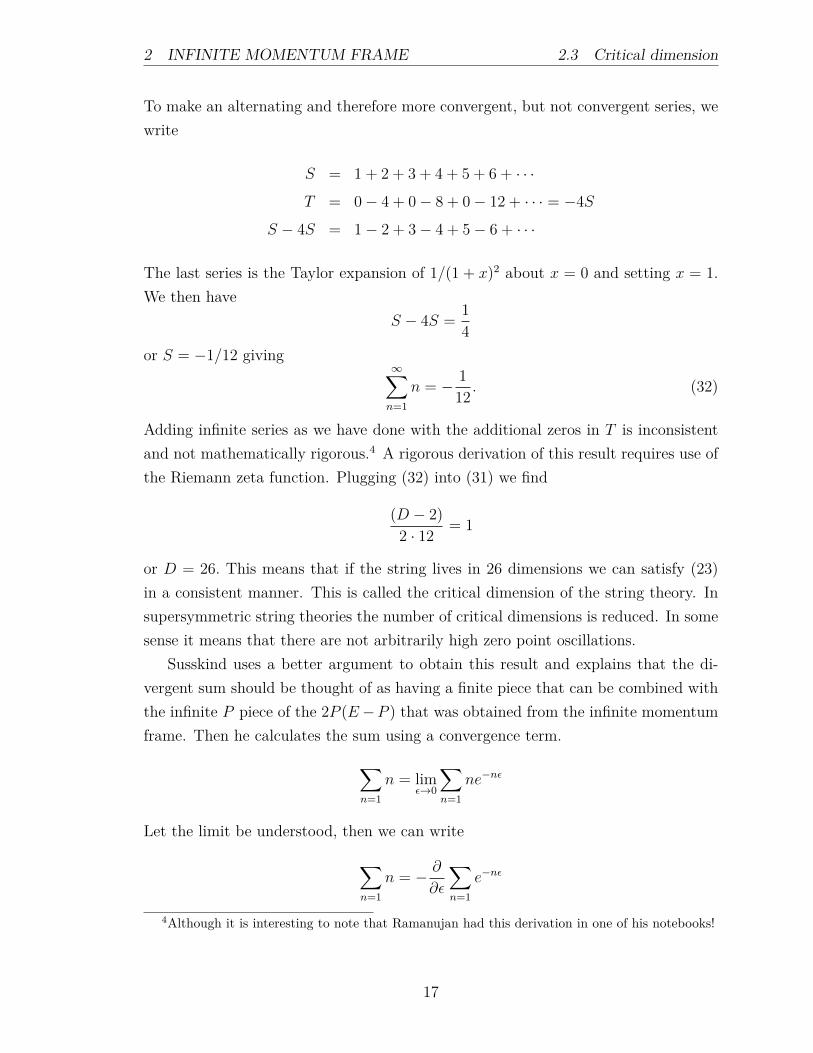
or D = 26. This means that if the string lives in 26 dimensions we can satisfy (23)in a consistent manner. This is called the critical dimension of the string theory. Insupersymmetric string theories the number of critical dimensions is reduced. In somesense it means that there are not arbitrarily high zero point oscillations.

Susskind uses a better argument to obtain this result and explains that the di-vergent sum should be thought of as having a finite piece that can be combined withthe infinite P piece of the 2P (E−P ) that was obtained from the infinite momentumframe. Then he calculates the sum using a convergence term.∑

n=1

n = limε→0

∑n=1

ne−nε

Let the limit be understood, then we can write

∑n=1

n = − ∂

∂ε

∑n=1

e−nε

4Although it is interesting to note that Ramanujan had this derivation in one of his notebooks!

17

3 OPEN STRING SCATTERING

where we note that the sum starts from n = 1. Performing the sum gives e−ε/(1−e−ε)

and expanding the exponentials to third order gives

− ∂

∂ε

[(1− ε+ ε2/2− ε3/6)

(ε− ε2/2 + ε3/6− ε4/24)

]= − ∂

∂ε

[1

ε

(1− ε+ ε2/2− ε3/6)(1− ε/2 + ε2/6− ε3/24)

].

Keeping terms to order ε2, and using 1/(1− x) = 1 + x+ x2 + · · · , gives

− ∂

∂ε

[1

ε

(1− ε+ ε2/2

) (1 + ε/2− ε2/6 + ε2/4

)]where the ε2/4 comes from (ε/2− ε2/6)2, the x2 in the expansion. Then we have

− ∂

∂ε

[1

ε

(1− ε/2 + ε2/12

)]−→ lim

ε→0

1

ε2− 1

12

which contains the formally infinite piece (infinity!) plus the finite piece −1/12.The fermionic string reduces the number of required dimensions to D=10, and

removes the tachyon states.

3 Open String Scattering

3.1 Mandelstam variables

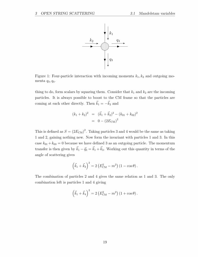
In particle scattering analysis it is useful to define the Mandelstam variables. Considera 4-particle scattering event with four identical particles with incoming and outgoingfour-momenta k1, k2, q3, q4. Momentum and energy conservation dictate that wewrite k1 + k2 = q3 + q4. If we relabel q3 = −k3 and q4 = −k4 we have

k1 + k2 + k3 + k4 = 0.

In this case, the figure would show all lines going in to the blob. The Klein-Gordonrelation can be written p2 − E2 = kµk

µ = −m2 for each of the particle and provideconstraints. There are 16 independent variables in the four-momenta of each of theparticles. The constraint equations reduce the number of independent variables tojust two. In the center of mass frame there are ultimately only two variables thatdescribe the amplitude of scattering, the total energy ECM, and the angle throughwhich the scattered particles depart, θ. There is only one relevant angle if all fourparticles are identical. To form invariants from the four-momenta there is only one

18

3 OPEN STRING SCATTERING 3.1 Mandelstam variables

k1

k2

q3

q4

Figure 1: Four-particle interaction with incoming momenta k1, k2 and outgoing mo-menta q3, q4.

thing to do, form scalars by squaring them. Consider that k1 and k2 are the incomingparticles. It is always possible to boost to the CM frame so that the particles arecoming at each other directly. Then ~k1 = −~k2 and

(k1 + k2)2 = (~k1 + ~k2)

2 − (k01 + k02)2

= 0− (2ECM)2

This is defined as S = (2ECM)2. Taking particles 3 and 4 would be the same as taking1 and 2, gaining nothing new. Now form the invariant with particles 1 and 3. In thiscase k01+k03 = 0 because we have defined 3 as an outgoing particle. The momentumtransfer is then given by ~k1− ~q3 = ~k1 +~k3. Working out this quantity in terms of theangle of scattering gives(

~k1 + ~k3

)2= 2

(E2

CM −m2)(1− cos θ) .

The combination of particles 2 and 4 gives the same relation as 1 and 3. The onlycombination left is particles 1 and 4 giving(

~k1 + ~k4

)2= 2

(E2

CM −m2)(1 + cos θ) .

19

3.1 Mandelstam variables 3 OPEN STRING SCATTERING

k2 k4

k1 k3

k1 k3

k2 k4

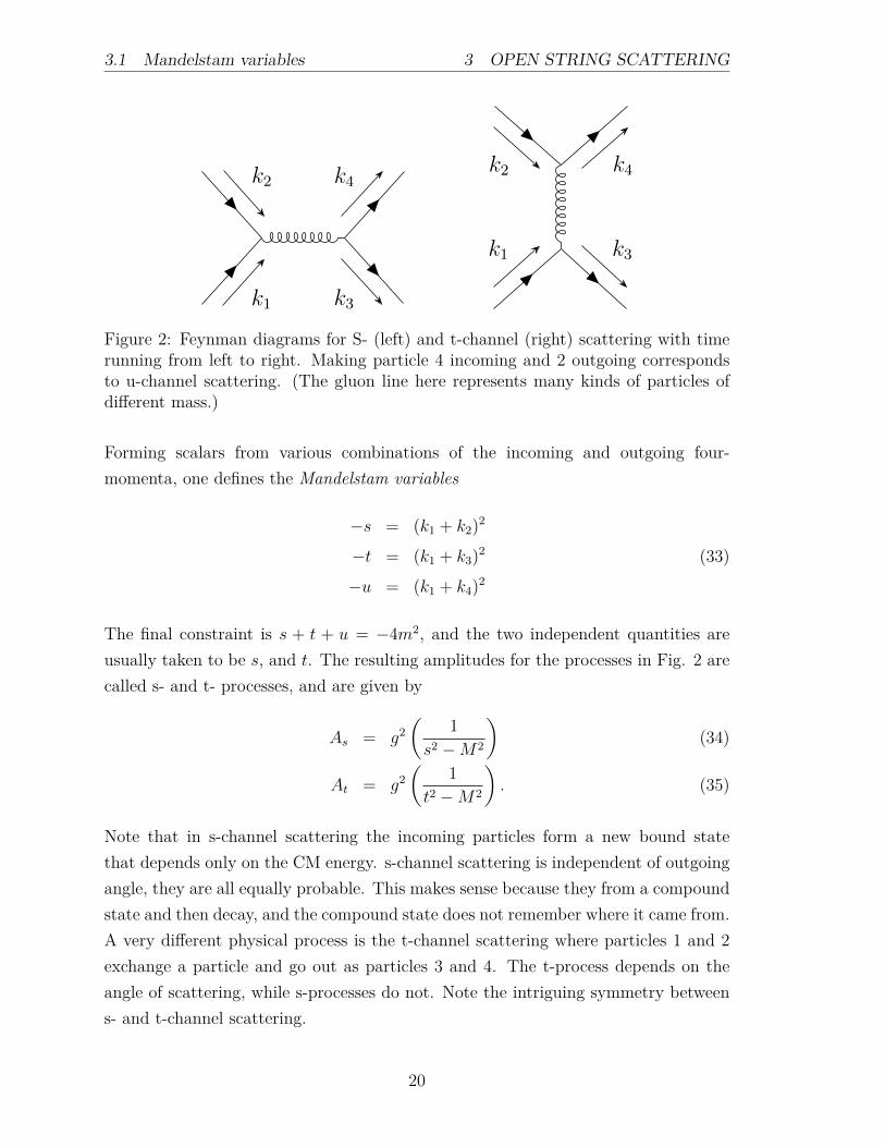
Figure 2: Feynman diagrams for S- (left) and t-channel (right) scattering with timerunning from left to right. Making particle 4 incoming and 2 outgoing correspondsto u-channel scattering. (The gluon line here represents many kinds of particles ofdifferent mass.)

Forming scalars from various combinations of the incoming and outgoing four-momenta, one defines the Mandelstam variables

−s = (k1 + k2)2

−t = (k1 + k3)2 (33)

−u = (k1 + k4)2

The final constraint is s + t + u = −4m2, and the two independent quantities areusually taken to be s, and t. The resulting amplitudes for the processes in Fig. 2 arecalled s- and t- processes, and are given by

As = g2(

1

s2 −M2

)(34)

At = g2(

1

t2 −M2

). (35)

Note that in s-channel scattering the incoming particles form a new bound statethat depends only on the CM energy. s-channel scattering is independent of outgoingangle, they are all equally probable. This makes sense because they from a compoundstate and then decay, and the compound state does not remember where it came from.A very different physical process is the t-channel scattering where particles 1 and 2exchange a particle and go out as particles 3 and 4. The t-process depends on theangle of scattering, while s-processes do not. Note the intriguing symmetry betweens- and t-channel scattering.

20

3 OPEN STRING SCATTERING 3.2 The Veneziano amplitude

Figure 3: Bosonic open string scattering. Two open strings come together for a timeτ and then separate. Time runs from left to right in this figure.

3.2 The Veneziano amplitude

Historically in the 1960’s when meson scattering amplitudes were first being measured,the two amplitudes for s- and t-channel scattering were thought to add in a calculationof the amplitude. But the scattering amplitude from this calculation is twice whatis seen in experiments. Physicists at the time were trying various functions for theamplitude that might result from an exchange of a large number of particles in thechannels. The result was that one was discovered that matched the data perfectly,and has the same symmetry as the diagrams. It is called the Veneziano amplitudeand is given by

AVeneziano = g2Γ(−s)Γ(−t)Γ(−s− t)

. (36)

How one arrives at the Veneziano amplitude from first principles is a triumph of stringtheory. The calculation goes as follows.

3.3 Bosonic open string scattering

We now consider two strings as shown in Fig. 3. Two strings moving freely throughspace come together and joint for a time τ . We need to calculate the scatteringamplitude for this process. We take the top string to have incoming momentum k1

and the bottom string incoming momentum to be k2. We write the wave function ofthe top string in the ground state of all the harmonic oscillators that make up thestring as

ψt(k1;x1, · · · , xN) = eik11N

∑Nn=1 xnψ0(x1, x2, · · · )

21

3.3 Bosonic open string scattering 3 OPEN STRING SCATTERING

where xl is the position of the l-th mass point on the string. Do not confuse this withthe Fourier mode decomposition above where we quantized. The bottom string as

ψb(k2;xN+1, · · · , x2N) = eik21N

∑2Nn=N+1 xnψ0(xN+1, xN+2, · · · ).

The state ψ0 is the wave function of a collection of harmonic oscillators in theirground states and is just a product of exponentials.Note that the CM is given byxCM = 1

N

∑Nn=1 xn; we describe the momentum state of the string in terms of the

motion of the center of mass. The crucial point in this analysis is the following. Forthe time period in which the strings are attached, we set xN = xN+1, providing aconstraint, and describe the wave function of the combined strings as

Ψ(k1, k2;x1, · · · , xN , xN , xN+1, · · · , x2N) =

eik1

1N

(xN+1+

∑N−1n=1 xn

)eik2

1N

∑2Nn=N+1 xnψ0(x1, x2, · · · , xN)ψ0(xN , xN+2, · · · ). (37)

At this point we must evolve the system in time using the Hamiltonian, Ψ(τ) =

e−iHτΨ(0), which we have already expressed above. The amplitude for the event isgiven by projecting the time-evolved state Ψ(τ) onto the disconnected string stateswith outgoing momenta k3 and k4. According to the Feynman rules we must calculatethe amplitude5 by summing the projection for all possible times τ , giving

A =

∫ ∞

0

dτ ψ(k3, x1, · · · , xN)ψ(k4, xN+1, · · · , x2N) e−iHτΨ(0). (38)

One can approach the calculation of eiHτΨ(0) by considering a few simple cases.First, a one-dimensional quantum harmonic oscillator has ground state wave functionφ0(x) = αe−mωx2/2 with α = (mω/π)1/4. This is a stationary state so Hφ0 = ω

2φ0,

and e−iHτφ0 = e−iωτ/2φ0. In the case of the string we have a collection of mass pointsconnected by springs and the Hamiltonian is given by

H =1

2m

N∑l

x2l +1

2mω2

N∑l

(xl+1 − xl)2 .

5A path integral calculation of the scattering amplitude would involve an integral over all of thetrajectories Xµ(τ) for each of the mass points. Then the amplitude would be something like

A =

∫[DXµ] e−

∫dτ L

where exponential is the Wick-rotated action for the interacting strings.

22

3 OPEN STRING SCATTERING 3.3 Bosonic open string scattering

Focus on the mass point located at xl. This piece of the Hamiltonian will be

hl =1

2mx2l +

1

2mω2

[(xl − xl−1)

2 + (xl+1 − xl)2]

= − 1

2m∂2l +

1

2mω2

(∆2

l−1,l +∆2l,l+1

)where we have defined ∆l,l−1 = xl − xl−1. The wave function for the string is

Ψ = eik(···+xl−1+xl+xl+1+··· )/Ne−mω

2

[···+(xl+1−xl)

2+(xl−xl−1)2+···

](39)

We need the action of the Hamiltonian on this piece of string moving with a momen-tum k, i.e.

e−ihlτΨ(0)

so we needhle

ik(···+xl+··· )/Ne−mω

2

(···+(xl−xl−1)

2+(xl+1−xl)2+···

)

to give us an eigenvalue so that the full exponential e−ih1τψ = e−i(eval)τψ. Calculating,we have

e(all that) ≡ eik(···+xl+··· )/Ne−mω

2

(···+∆2

l−1,l+∆2l,l+1+···

)∂le

(all that) = e(all that) [+mω∆l−1,l −mω∆l,l+1 + ik/N ]

∂2l e(all that) = e(all that)×

[+mω (∆l−1,l −∆l,l+1) + ik/N ]2 − 2mω

so that

hle(all that) =

(− 1

2m∂2l +

1

2mω2

[∆2

l−1,l +∆2l,l+1

])e(all that) =

+mω2∆l−1,l∆l,l+1 + ik

Nω (∆l−1,l −∆l,l+1) +

k2

2N2m+ ω

In the limit N →∞ the spacing between points goes to zero, and ∆l,l±1 → 0, leavingus finally with the result

hle(all that) → k2

2N2m+ ω

so that we may writee−ih1τψ → e

−i(

k2

2N2m+ω

)τψ.

23

3.3 Bosonic open string scattering 3 OPEN STRING SCATTERING

We have N →∞ oscillators, giving

e−i

(k2

2N2m+ω

)Nτψ = e−i k2

2Nmτe−iNωτψ.

In the limit, the mass points go to zero such that Nm → 1 (a constant we define tobe unity), finally giving

e−i k2

2τe−iNωτψ

The wave function Ψ = ψtψb will have evolution

Ψ(τ) = e−iHτΨ(0) = e−iτ

[12(k1+k2)

2+Nω]Ψ(0).

Recall that s = − (k1 + k2)2. The amplitude we seek (38) will have another term

with (k3 + k4)2 and also has xN+1 = xN in the initial state before time evolution.

This particular term will give (k1 + k2 − k3)2. We still need to fill in the details here(Wick rotation?). If we Wick rotate, then the infinite term Nω gives e−Nωτ → 0 andwe are left with terms like e−τs. The calculation of the full amplitude (38) results in

A =

∫ ∞

0

dτ eτ(s+1) (1− eτ )−t−1 e−τ

which upon setting z = e−τ gives

A = −∫ 0

1

dz z−(s+1)(1− z)−t−1

=Γ(−s)Γ(−t)Γ(−s− t)

.

This is the Veneziano amplitude (36) for the scattering of two strings each in theirground state which we recall is a tachyon state. This function has a name in math-ematics, the Euler beta function β(a, b) ≡ Γ(a)Γ(b)/Γ(a + b). What we have justdemonstrated is remarkable; the scattering of two strings produces the amplitude ofs- or t-channel processes described by Veneziano for the scattering of mesons, anddoes so analytically. This strongly suggests that there is validity in the idea thatstrings are fundamental objects in nature.

Further confidence was gained by calculating the scattering amplitudes of thephoton-like and graviton-like (excited state) strings with themselves and with othertypes of string states. In QFT the scattering amplitudes of photon-photon andgraviton-graviton scattering are distinctive and string theory reproduces those am-

24

3 OPEN STRING SCATTERING 3.3 Bosonic open string scattering

plitudes.

3.3.1 Euler Beta functionThe beta function is defined as

β(n,m) =

∫ 1

0dl ln−1(1− l)m−1 (40)

We can construct a solution to this integral using the gamma function Γ(t) =∫∞o dt e−ttn−1. First we write the

product of two gamma functions.

Γ(n)Γ(m) =

∫ ∞

0dt e−ttn−1

∫ ∞

0dq e−qqm−1

We want to manipulate this integral to contain the beta integral in (40). We need to cover the right upper quadrantthat is represented by the integral over t and q. We will perform a coordinate transformation (t, q) → (z, l). To obtainthe correct measure we use differential forms with the substitutions

t → zl

q → z(1− l)

giving ∫ ∞

0dt

∫ ∞

0dq −→

∫ ∞

0dz

∫ 1

0f(z, l) dl

where we need to find the function f(z, l). The Jacobian can be calculated in the usual way. Here we’ll use differentialforms and write

dt = l dz + z dl

dq = dz − z dl − l dz

dt ∧ dq = (l dz + z dl) ∧ (dz − z dl − l dz)

= l dz ∧ dz − l dz ∧ z dl − l dz ∧ l dz

+ z dl ∧ dz − z dl ∧ z dl − z dl ∧ l dz

= −l dz ∧ z dl + z dl ∧ dz − z dl ∧ l dz

= −lz dz ∧ dl + z dl ∧ dz + zl dz ∧ dl

⇒ dt dq = z dl dz

Our double integral is transformed to

Γ(n)Γ(m) =

∫ ∞

0dz e−z zn+m−2 z

∫ 1

0dl ln−1(1− l)m−1

orΓ(n)Γ(m) = Γ(n+m)

∫ 1

0dl ln−1(1− l)m−1.

Finally we have the form of the beta function we desire∫ 1

0dl ln−1(1− l)m−1 =

Γ(n)Γ(m)

Γ(n+m).

The LHS is the beta function β(n,m). Note that when doing this manipulation the substitutions must follow the

25

4 WORLD SHEET SYMMETRIES

rules t+ q = z and t = z f(l), and g = z g(l), where f(l) and g(l) are functions of l. This allows the gamma functionto come out.

4 World sheet symmetries

The trajectory for a point particle is a world line xµ(λ) where λ is a parameter alongthe world line of the particle. A string sweeps out a world sheet. Each point alongthe string is parameterized by xµ(τ, σ). The path integral is written as∫

[Dx] eiS

with

S =1

2

∫dτ dσ

[(∂xµ

∂τ

)2

−(∂xµ

∂σ

)2]

(41)

In order to make the path integral converge we Wick rotate τ → −iτ .6 An integralover all surfaces is what defines the path integral for strings. For closed strings theworld sheet of a single string is a tube and interactions among closed strings look liketubes that join into larger tubes, and separate again. This is the generalization of asingle vertex in point particle QFT. If one allows the strings to have any arbitrarynumber of holes it becomes the generalization of the sum over all Feynman graphscontaining any number of loops and so on. So the path integral is a sum over allpossible surfaces that connect the starting positions and end positions of a set ofstrings.

The equation of motion for (41) yields the wave equation. After Wick rotationthe signs of the derivative terms are the same and the equation of motion will insteadbe the Laplace equation

∂x2µ

∂τ 2+∂2xµ

∂σ2= 0

The symmetries of the Laplace equation include reparameterization of the coor-dinates σ′ = (σ, τ) and τ ′ = (σ, τ). In particular, the kinds of coordinate transforma-tions that preserve the Laplace equation are conformally invariant transformations.Conformal transformations preserve angles, and infinitesimal squares are mapped

6The generic path integral in QFT is given by something like∫[Dx] ei

∫ t2t1

dt L(x,x) where theweight for each path is eiS(x) with S(x) =

∫ t2t1

dtL(x, x) and therefore has the same magnitude(they are points on the unit circle in the complex plane). Generally, this integral is hard to definemathematically and is non-convergent. The standard prescription is analytically continuing the pathintegral by setting t = iτ so that the path integral becomes

∫[Dx] e−

∫ −it2−it1

dτ L(x,x) = F (it1, it2) andthen analytically continuing the result back.

26

4 WORLD SHEET SYMMETRIES 4.1 Conformal mapping

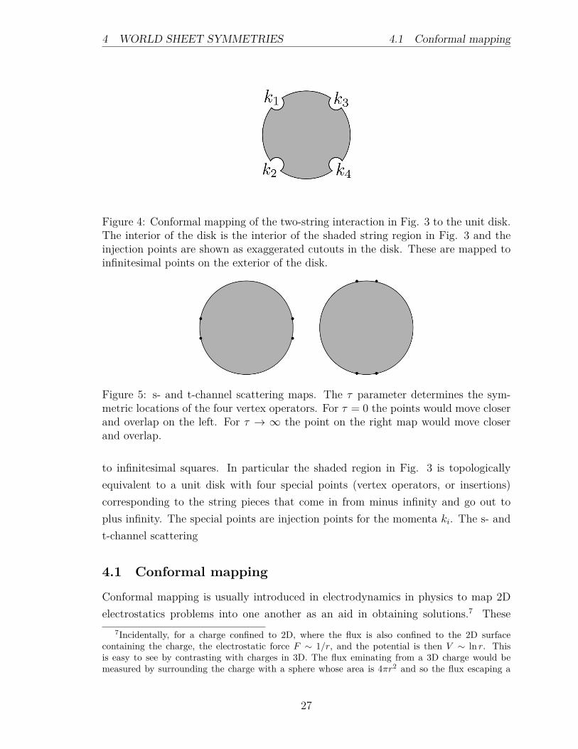
Figure 4: Conformal mapping of the two-string interaction in Fig. 3 to the unit disk.The interior of the disk is the interior of the shaded string region in Fig. 3 and theinjection points are shown as exaggerated cutouts in the disk. These are mapped toinfinitesimal points on the exterior of the disk.

Figure 5: s- and t-channel scattering maps. The τ parameter determines the sym-metric locations of the four vertex operators. For τ = 0 the points would move closerand overlap on the left. For τ → ∞ the point on the right map would move closerand overlap.

to infinitesimal squares. In particular the shaded region in Fig. 3 is topologicallyequivalent to a unit disk with four special points (vertex operators, or insertions)corresponding to the string pieces that come in from minus infinity and go out toplus infinity. The special points are injection points for the momenta ki. The s- andt-channel scattering

4.1 Conformal mapping

Conformal mapping is usually introduced in electrodynamics in physics to map 2Delectrostatics problems into one another as an aid in obtaining solutions.7 These

7Incidentally, for a charge confined to 2D, where the flux is also confined to the 2D surfacecontaining the charge, the electrostatic force F ∼ 1/r, and the potential is then V ∼ ln r. Thisis easy to see by contrasting with charges in 3D. The flux eminating from a 3D charge would bemeasured by surrounding the charge with a sphere whose area is 4πr2 and so the flux escaping a

27

4.1 Conformal mapping 4 WORLD SHEET SYMMETRIES

techniques are standard methods used in elementary complex variables so we willsummarize the basics quickly. Consider a mapping w(z) that takes the complex z

plane to the complex w plane. Where z = x + iy and w(z) = u(x, y) + iv(x, y). Weassume that the mapping is one-to-one and onto (bijective). In defining the derivativeof the mapping, w′(z) we examine the quantity

w′(z) =dw

dz=du+ idv

dx+ idy.

For the derivative to be uniquely defined, it must be the same if approached along anydirection in the z plane. It is easiest to come in along the x and y axes independently,so that dy = 0 and dx = 0, respectively. Setting these two derivatives equal yieldsthe Cauchy-Riemann equations

∂u

∂x=∂v

∂y

∂u

∂y= −∂v

∂x. (42)

Mappings that satisfy the Cauchy-Riemann equations are called analytic or holomor-phic. Setting the mixed partials of these equations equal shows that both of thefunctions u(x, y) and v(x, y) satisfy the Laplace equation, ∇2u = 0 and ∇2v = 0.

We will now show that any analytic mapping is a conformal mapping, i.e. itwill preserve angles. For this we consider two small arrows in the z plane, δz =

ρeiθ and ∆z = ρ′eiθ′ starting at the point z. The ratio of these displacements is

δz/∆z = (ρ/ρ′) ei(θ−θ′), indicating that the angle between these displacements is(θ − θ′). For an analytic mapping w(z), we stipulate that the derivative w′(z) exists.Then w(z + δz) = w(z) + δz w′(z) and w(z +∆z) = w(z) + ∆z w′(z). Therefore wehave the following ratios equal

δz

∆z=

δw

∆w

and the mapping is angle preserving. A few simple examples of analytic functionsare f(z) = z, and any power of zn, except 1/z, which has a pole at the origin, butis analytic everywhere else. Typical functions such as ez and sin(z), are analytic.An example of a non-analytic function is f(z) = z∗. It is easy to see that thisfunction does not satisfy the Caucy-Riemann equations. However, it is important instring theory to consider functions that are anti-analytic. These are functions thatare analytic in the variable z∗, often denoted with a bar as z. The Cauchy-Riemannequations for anti-analytic functions differ by a minus sign from the usual definition

small patch of area da on the sphere must be da/4πr2. In 2D, the flux would pass throug a circle of’area’ 2πr.

28

4 WORLD SHEET SYMMETRIES 4.1 Conformal mapping

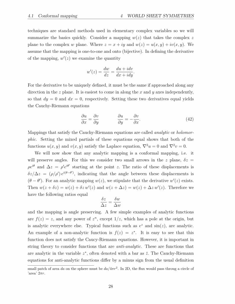
Figure 6: Linear fractional map w(z) = z+1z−1

.

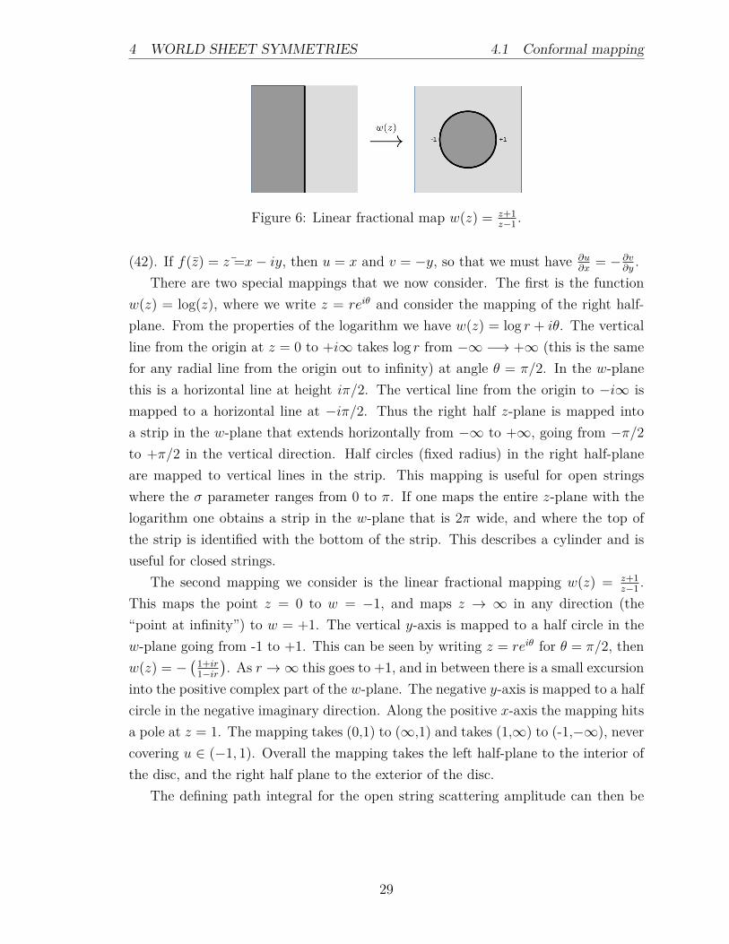
(42). If f(z) = ¯z =x− iy, then u = x and v = −y, so that we must have ∂u∂x

= −∂v∂y

.There are two special mappings that we now consider. The first is the function

w(z) = log(z), where we write z = reiθ and consider the mapping of the right half-plane. From the properties of the logarithm we have w(z) = log r + iθ. The verticalline from the origin at z = 0 to +i∞ takes log r from −∞ −→ +∞ (this is the samefor any radial line from the origin out to infinity) at angle θ = π/2. In the w-planethis is a horizontal line at height iπ/2. The vertical line from the origin to −i∞ ismapped to a horizontal line at −iπ/2. Thus the right half z-plane is mapped intoa strip in the w-plane that extends horizontally from −∞ to +∞, going from −π/2to +π/2 in the vertical direction. Half circles (fixed radius) in the right half-planeare mapped to vertical lines in the strip. This mapping is useful for open stringswhere the σ parameter ranges from 0 to π. If one maps the entire z-plane with thelogarithm one obtains a strip in the w-plane that is 2π wide, and where the top ofthe strip is identified with the bottom of the strip. This describes a cylinder and isuseful for closed strings.

The second mapping we consider is the linear fractional mapping w(z) = z+1z−1

.This maps the point z = 0 to w = −1, and maps z → ∞ in any direction (the“point at infinity”) to w = +1. The vertical y-axis is mapped to a half circle in thew-plane going from -1 to +1. This can be seen by writing z = reiθ for θ = π/2, thenw(z) = −

(1+ir1−ir

). As r →∞ this goes to +1, and in between there is a small excursion

into the positive complex part of the w-plane. The negative y-axis is mapped to a halfcircle in the negative imaginary direction. Along the positive x-axis the mapping hitsa pole at z = 1. The mapping takes (0,1) to (∞,1) and takes (1,∞) to (-1,−∞), nevercovering u ∈ (−1, 1). Overall the mapping takes the left half-plane to the interior ofthe disc, and the right half plane to the exterior of the disc.

The defining path integral for the open string scattering amplitude can then be

29

4.1 Conformal mapping 4 WORLD SHEET SYMMETRIES

written as

A =

∫ (∏j

dzj

)∫DX e

−∫dτdσ

[∂Xµ∂τ

∂Xµ

∂τ+

∂Xµ∂σ

∂Xµ

∂σ

]∏j

eik(j)µ Xµ(~z) (43)

where the integral over the zj is the integral of the vertex operator positions on theboundary of the unit disc that inject strings of momentum k(j) into the world sheet.By conformal mapping three of these positions can be fixed, but the rest must beintegrated over. The number of vertex opertors corresponds to the number of stringsinteracting. This is a genus 0 sheet, it captures all s- and t-processes and anythingthat can be deformed topologically without tearing the sheet. So this takes care ofall tree-level processes.

The action in (43) is conformally invariant and the equation of motion for eachfield Xµ satisfies the Laplace equation. The path integrals are all Gaussian and canbe done independently for each of the 26 fields. The problem is therefore reducedto solving the Laplace equation on the disc with the charges being the k(j)µ . In thecase where there are four strings interacting, we have k(1)µ , · · · , k(4)µ and 26 kinds of“charge,” one for each dimension. What is being calculated is the analog of theelectrostatic energy for each field Xµ. The final result is that the amplitude is givenby

A =

∫ (∏j

dzj

)e−

∑j Ej(~z) (44)

where Ej(~z) is the energy of the j-th type charge which depends on the locations ofall the other injected charges of the same type. This is the simplest form of openstring theory and (43) can be taken as a definition of this theory.

This result (44) is calculated for strings in 26 dimensions and the mathematicsso far has been relatively simple. The real complexity in string theory comes inwith the compactification of these extra dimensions to leave only the 3+1 dimensionsthat we see. The number of ways of compacting these dimensions is very subtleand mathematically difficult. The compactification allows one to put gauge groupsymmetries into string theory thus giving a connection the Standard Model. However,the number of ways of compactifying results in a large number of possible “standardmodels” of the order 10500. The current problem with string theory is that thereseems to be no way of picking one and that they may occur randomly.

30

4 WORLD SHEET SYMMETRIES 4.2 Compactification

4.2 Compactification

Let us contrast the difference between a point particle and a string moving on a surfaceembedded in a large flat space. A point particle that is constrained to remain in thesurface with no other forces on the particle will move along a geodesic. Classically,we can divide up the trajectory of the particle into small pieces, and in the limit wehave a continuous line. Quantum mechanically the picture is different.

On a sphere of radius R a point particle with no other forces would travel on agreat circle. The energy of the center of mass of the particle would be mv2/2 = p2/2m.Because the angular momentum is quantized, and because L = mvR = pR, we havethat

E = L2/2mR2

= L2/I, (45)

where the moment of inertia is I = mR2. For a string moving on the geometry of asphere things are much different. We have to consider the spatial extent of the stringdue to its zero point motion. We could calculate the root mean square by calculatingXrms =

√〈0|X2(σ)|0〉. Using the creation and annihilation operators we have

〈0|∑nn′

1√n√n′

(a+n + a−n

) (a+n′ + a−n′

)|0〉

and the only contributing term will be a−n a+n′ with n = n′. This will give∑

n1n

whichis formally divergent. Again we regulate the sum using a cutoff

∑nmaxn and look for

the dependency of the energy in (45) on the regulator. The integral approximation tothe sum is

∑nmaxn ∼ ln(nmax). On a sphere, when the higher ZP modes are included

in the string Xrms begins to cover the surface of the sphere and the CM of this “stringtangle” moves closer to the center of the sphere and in the limit of including all themodes we find I → 0, and (45) becomes divergent. We interpret this to mean thatstring motion in this geometry is not allowed; the sphere is a bad geometry for stringsto move in. In order to find a suitable geometry we have to consider the metric, gµν(x),of the surface it moves in. Because the string itself has energy and can deform themetric of the space, we need the change in the metric of the space to be well-behavedwith the regulator introduced above. This will require that the space be “Ricci flat.”We can write this as

δgµν = R αµνα = Rµν . (46)

31

4.2 Compactification 4 WORLD SHEET SYMMETRIES

This is the variation of the metric with a change in the regulator. We want this tobe zero.

δgµν = Rµν = 0 (47)

Now consider the Einstein equations for the vacuum,8

Rµν −1

2gµνR = 0.

The scalar curvature R = Rαα is the trace of the Ricci tensor. Raising one index in

the free field equation we have

Rµνgνα − 1

2gµνg

ναR = 0

Rαµ −

1

2g αµ R = 0

Rαµ −

1

2δ αµ R = 0.

Now form the trace by setting α = µ and summing, giving

R− 4

2R = 0

R = 2R.

Clearly this can be satisfied only for R = 0, or the space is Ricci flat. This means thatthe consistency condition (46) for strings moving in a spacetime background requiresthat the background space be a solution of the free field Einstein equations. This isremarkable.

Compactification of a surface can be done many ways, and we begin with anexample of a 2D spatial sheet of finite extent. If we take a rectangle and identifythe left side with the right side we obtain a cylinder. If we take the same rectangleand identify the lhs with the rhs and the top with the bottom, we obtain a torus.Topologically the two are identical if we remember the identifications required on therectangle. If we start with a 3D rectangular parallelopiped, infinite in one direction,and identify the front with the back and the top with the bottom (the compact

8The full Einstein field equations have the energy-momentum tensor Tµν on the rhs that containsmatter and everything other than the gravitational field. Solutions to the vacuum equations include,in particular, gravitational waves, e.g. think about the vacuum Maxwell equations that admit wavesolutions. Other “solutions” include Schwarzchild, and FRW, but those have singularities. The deSitter spaces are solutions to the vacuum equations provided there is an additional cosmologicalconstant term.

32

4 WORLD SHEET SYMMETRIES 4.3 Winding number

directions), we have a torus at each point of the non-compact direction. This can beimagined as a 1D line with a torus attached at each point of the line. Similarly wecould imagine another topology consisting of a line with a sphere attached at eachpoint of the line. However, we have seen above that a sphere is not a good geometryfor strings to move on. Toroids are the simplest and most direct way to compactifydimensions, and this process is called “toroidal compactification.”

There are three parameters that describe a 2-torus. If we unwrap a 2-torus wefirst cut it and unwrap it to form a cylinder, and then cut the cylinder lengthwise toa rectangle of sides a and b. The three parameters are (1) the area ab, also called theKahler modulus, (2) the ratio of the sides a/b, is the complex structure modulus, and(3) the identification “angle” or parameter that describes any twist applied to thecylinder before reconnecting it to form the 2-torus is called the Dehn twist. Theseare called the moduli, and make up the moduli space of the torus.9

Other Ricci flat manifolds called Calabi-Yao manifolds are good manifolds forstrings to move on. They appear to provide more of a connection to the particlephysics we know because they are less symmetric than tori, and the tori are toosymmetric.

4.3 Energy spectrum and winding number

Consider a point particle moving on a 2D surface which is compact in one dimension,e.g. a long cylinder of radius r. It can have two components of momentum, onealong the non-compact direction and one along the compact direction. Momentumalong the compact direction is quantized. This can be seen using the usual periodicboundary condition for a plane wave, eikx = eik(x+2πr), and so 2πkr = 2πn for someinteger n. Therefore km = n/r. For a massless particle E = |p|, and so E ∼ n/r forn ∈ Z. Because energy is mass, the mass spectrum of these particles will have spacing1/r. As r →∞, then the spacing between the states is very small. This particle canalso be a string of small spread.

Now consider a string wrapped around the compact dimension. Its length has anenergy density, so the number of times the string is wrapped around the compactdimension gives its energy, and this goes as nr, where n is called the winding number.Negative n correspond to the direction in which the string is wound. So we havetwo types of mass spectra, the non-wound string that goes as n/r, and the wound

9There are non-orientable surfaces such as the Klein bottle that can be made by identifying thecylinder edges before reconnecting, but they are not good surfaces for strings to move on. Thesurfaces must be Ricci flat.

33

4.3 Winding number 4 WORLD SHEET SYMMETRIES

string that goes as nr. Note that the spectrum of these two pictures exchange andgo into each other as r → 0 or r → ∞. These pictures are dual to each otherby exchanging the n of the quantized momentum with the winding number andexchanging r ←→ 1/r. This is a symmetry of the theory. At the radius r = 1

the spectra are the same. As one reduces the compact dimension length scale belowr < 1, the non-wound theory just looks like the string theory with winding numberin a space with r > 1.10 This is called T-duality where the T is for torus.

The winding number is a conserved quantity. To show this we remember thatfor closed oriented strings, there is a sense of direction along the string. Take twostrings of winding number w = 1 and w = −1 wrapped around the compact directionin opposite directions. If the strings are allowed to interact and combine, we mustfollow the rule that the sense of direction of a string cannot change along the string.Then when the strings combine, the only way for them to do so is to form one stringthat is no longer wound around the compact direction. The total winding number 0is conserved. Drawing a picture is easy and it will be obvious. If instead we wraptwo strings both with w = 1, and let them combine to form one string it is easy tosee that the winding number of the single string is 2.

The mathematics of the T-duality can be described as follows. For an unwoundstring with (quantized) momentum along the compact direction we write E = p =

n/r, but p ∼ dy/dτ where y(σ) is the coordinate in the compact direction at thepoint σ along the string. So we can write

n = r

∫dσdy(σ)

dτ

where the integral over dσ accounts for different parts of the string moving at differentvelocity. Similarly, we can consider the winding number of a string. The coordinatealong the string σ goes from 0 → 2π for a closed string. The circumference of thecompact space coordinate is 2πr, therefore we can write σ = y/r so that as y goesfrom 0→ 2πr, σ goes from 0→ 2π. Here the energy E = w2πr is proportional to rand we write

w =1

r

∫dσdy(σ)

dσ.

T-duality takes n→ w, r → 1/r, τ → σ.10This implies that there is a smallest length scale.

34

5 KALUZA-KLEIN

5 The Kaluza-Klein Picture

Closed strings on a compact manifold exhibit repulsion and attraction; they behavelike charged particles. If two strings attract or repel each other in this way it isnatural to ask how. For simplicity we consider 5 dimensions, one time and fourspace, one of which is compact. This is the Kaluza-Klein (KK) picture that is able tocombine electromagnetism with general relativity. The mathematics is also used instring theory. Here we are considering closed strings. We will see that closed stringswith momentum number +n in the compact direction attract those with momentumnumber −n, and likewise for strings with winding number +w and −w. Repulsionoccurs between objects whose momentum number or winding number is the samesign.

5.1 Kaluza-Klein metric

The generalization to an extra compact dimension of space was first proposed byKaluza and later refined by Klein. The idea is simple. Instead of the usual GRmetric gµν where µ, ν ∈ 0, 1, 2, 3 we define a more general metric tensor

gMN =

(gµν gµ5

gµ5 g55

). (48)

We want to find an analog electric or magnetic field to describe the attraction andrepulsion of these strings. Recall from electromagnetism that the fundamental objectis the vector potential Aµ = (φ,A1, A2, A3) where ~B = ∇× ~A, and ~E = −∇·φ−∂t ~A.The vector potential Aµ is a four-vector. The photon is a vector particle and hasa vector index corresponding to the µ. The KK metric tensor contains two newfields, gµ5, a four-vector that can be identified with Aµ, and g55, a scalar Φ called thedilaton. The dilaton or g55 is the component of the metric around the 5-th directionand tells you how big the 5-th direction is. If g55 is big or small, then so is the 5-thdirection. Both new fields are functions of the spacetime coordinates gµ5 = gµ5(x)

and g55 = g55(x). If g55 can vary, then the compact dimension can vary and looks likea tube of varying radius. These represent waves in the compact direction or particlesassociated with the dilaton. The quiescent vacuum would have no such waves andthe radius would be constant.

Recall the definition of the energy-momentum tensor Tµν , the time componentsT0j correspond to the momentum flow in each spatial direction. In the KK metric the

35

5.1 Kaluza-Klein metric 5 KALUZA-KLEIN

terms gµ5 correspond to momentum flow in the 5-direction. The source of the analogvector potential is the component of momentum going around the 5-direction. Themomentum quantum number ±n can be though of as electric charge corresponding tothe vector field gµ5. This electric field is associated with the graviton. The momentumnumber n, and the winding number w correspond to two kinds of electric charge,giving rise to n-photons, and w-photons. Momentum photons are a piece of thegravitational field gµ5, gravitons which are polarized along the µ5-direction. The moregeneral picture including photons emitted and absorbed by the winding number areas follows. Recall the spectrum of closed strings where we had to use level matching.The creation and annihilation operators can now create oscillations in the usual threedirections of the non-compact space. These are

(ai±n

)± where i ∈ x1, x2, x3 andthe left and right operators are given by ±n. The tachyon has -2 units of energy andwe ignore it. To get a non-tachyonic state we must create two units of energy andform states like ai+−1a

j++1 |0〉, corresponding to gravitons polarized in two directions in

space. We can also form excitations like ai+−1a5++1 |0〉, which has one index and can

be identified with the polarization of the photon since we have only one index inthis state. We can also form ai++1a

5+−1 |0〉. The correct thing to do is to form linear

superpositions and form two kinds of photon fields

(ai++1a

5+−1 ± ai+−1a

5++1

)|0〉

where + ↔ n-photons, and − ↔ w-photons. The n-photons are identified with gµ5,gravitons, and the Ramond field bµ5 is associated with the w-photons or winding num-ber. There is also a combination of creation operators that have no index structureand correspond to a scalar particle, a5++1a

5+−1 |0〉, the field quanta of the dilaton field Φ.

T-duality can be stated

n↔ w

r ↔ 1/r

∂x/∂τ ↔ ∂x/∂σ

gµ5 ↔ bµ5.

At the moment these are mathematical constructions and real particle candidates arenot known for all of these particles. However, there is plenty of room in physics forthese objects.

36

5 KALUZA-KLEIN 5.2 D-branes

5.2 D-branes

T-duality for open strings leads to the idea of Dirichlet branes or D-branes, discoveredby Polchinski. The D-branes can have different dimensions and a Dn-brane hasn dimensions. Consider the space R3 × S1 where the compact space is S1 withcoordinate y and take it to be very small. Suppose a string lives in this space. TheNeumann boundary condition on the string is ∂y/∂σ|0,π = 0, which means there is nostretch of the string at the very endpoints. If we insist that T-duality holds for thestring, then in the dual space where S1 is very large we have the dual condition that∂y/∂τ |σ=0,π = 0, or that the string end points cannot move; the string is pinned inthe S1 space. This object that has dimension 1 anchors the end of the string and canbe thought of as a 1-dimensional object that is heavy, because strings attached to itcannot leave it. These objects have to be deformable to make sense from a generalrelativistic point of view, and so they are objects that have their own dynamics.A D0-brane is a point, a D1-brane is a string (though it is heavy and not like thestrings that are attached to it). A D2-brane is a membrane, and a D3-brane is a3-dimensional space where strings attach. If we think about open string theory in our3-dimensional world we would say the strings are attached to a space-filling D3-branewhere they move all about the space because the endpoints are attached to the wholespace. One can say that open string theory in which T-duality is imposed predictsD-branes.

The strings attached to a D-brane have an orientation that gives rules for joiningand breaking of strings for scattering amplitudes. Each string attached to a branehas an arrow along its length. If two strings attached to a D2-brane approach eachother the only ends that can join are the two of opposite orientation. In other wordstwo strings cannot join that have arrows coming out of the points. That would leadto a string that had two arrows along its length of opposite direction. This leads tostrings conserving orientation number.

QCD has a beautiful connection to D-branes and string theory in the followingsense. Consider three separate D3-branes labeled R, G, B that are embedded in ahigher dimensional space. Then a string attached to the R3-brane has points labeledr, r, where one has an arrow going into the brane and the other an arrow going out.Strings can attach at one brane and go to another type of brane so there could berb strings, and so forth. Incidentally there are 8 gluons and not 9 because one linearcombination can come together and disappear. For example the ends of an rr gluoncan come together and lift off the sheet and thus is not stable. An isolated quark inthis picture would be a string that starts one of the RGB sheets and goes off to some

37

6 FUNDAMENTAL OBJECTS

distant other brane of a different kind. These rules are the same as super Yang-MillsQCD rules.

Supposing we have only one D3-brane the structure of the theory is like electro-magnetism. In this picture a string with both ends attached to the brane is a photonlike object, and a string with one end in the brane and one end at infinity is a anelectron. A positron would have the opposite orientation. The theory predicts in thispicture that a D1-brane that ends on the D3-brane is a magnetic monopole. It isheavier than the usual string that ends on the D3-brane that represents the electronor positron.

Finally, if open strings are attached to D-branes, and if our physical world isa D3-brane with open strings attached. Then open strings may describe all of theStandard Model particles, and closed strings which do not attach to these branes maydescribe the gravitons. These gravitons can wander freely over all of the spaces andthis may explain why gravitational forces are so much weaker than the others; gravitycan “leak out” into the other dimensions.

Part II

Topics in String TheoryThis part of the document follows the first several lectures of Susskind’s “Topics inString Theory” lectures.

6 Fundamental Objects

In quantum field theory there is a well-known picture associated with bosonizationthat indicates there is difficulty in determining what objects are fundamental or not.Consider two spin-1/2 fermions with coupling g. A field ψ describes the fermion field.If g 1 then the fermions move freely and are considered the fundamental particles.If the coupling is very strong, g 1, then the fermions look like a composite particlethat can have a ground state of spin 0 and look like a boson. In this picture theboson would be considered the fundamental particle. The boson field φ is an effectivedescription of the fermions. The boson field creates pairs of fermions. The bosonscannot be paired together to look like fermions because any pair of two bosons is alsoa boson. However, there is a completely different way to think about the fermions in

38

6 FUNDAMENTAL OBJECTS 6.1 The electron and the monopole

terms of the bosons in terms of kinks in the boson field. The field φ smoothly jumpsover some small distance. A good example is a belt that is twisted 2π over some smalldistance. Kinks are heavier than the bosons that make up excitations in the field φ,and these kinks behave like fermions.

For some ranges of the parameters in the field theories ψ and φ it is easier tothink of ψ is the fundamental field and its building blocks are fundamental, and forother parameters of the field theory the bosons are more useful to think of as thefundamental objects. Here the bosons would behave more simply for example.

6.1 The electron and the monopole

A more sophisticated example is given by quantum electrodynamics. Here we thinkof the electron as a fundamental particle. The fine structure constant α ∼ e2, witha numerical value of ≈ 1/137, is the coupling constant that describes the probabilityof an electron emitting a photon if it is accelerated. The electron only emits photonsperhaps 1% of the time. It takes very large energies to probe the structure of theelectron and infer the cloud of virtual photons and e+e− pairs that surround it. FromDirac’s famous calculation of the charge of the magnetic monopole, g = 2π/e, we seethat the magnetic monopole will interact with photons much more strongly. In doingso there will be a complicated cloud of virtual photons, and electron-positron pairsthat surround it. The monopole is therefore much heavier than the electron. If weconsider the electric charge e as a parameter, then as we vary the parameter fromvery small to very large, the electron and the monopole trade places in the complexityof the cloud that surrounds them. The monopole would become very light and theelectron very heavy. It is therefore not entirely clear then what object is consideredfundamental.

6.2 D-branes and S-duality

In string theory the presence of D-branes is part of the mathematical framework andthese objects must exist as discussed in the section above. We will now discuss twoversions of string theory. In one theory there are only even dimensional D-branes andin the other only odd dimensional D-branes. If we consider first the odd dimensionalversion, then there are no D0-branes, but there are D1-branes which we discussedas being much heavier than fundamental strings. In string theory the parameterthat allows for duality is the string coupling constant, g. This constant controls theprobability of strings breaking and connecting.

39

6.2 D-branes and S-duality 6 FUNDAMENTAL OBJECTS

In a theory that contains D1 branes the same behavior is present, the D1 stringhas lots of fundamental strings (F-strings) attached to it, and so it is a heavy object.In this type of theory a fundamental string and a D1 string will morph into each otherbased on the value of the coupling constant g of the theory. If g 1 the F-strings arevery light. As g becomes large the F-string gets heavier and so the D1 string cannot“emit” as many F-strings and so it starts to look more simple. At the same time anybits of string that break off from the F-string will form closed loops and be attractedaround the F-string. The closed loops form the particles like the graviton, etc. Asg 1 these become very massive and turn into black holes. The D1 strings thenget lighter and they make up the gravitons. This is called S-duality for “strengthduality”, the strength of the coupling constant. In string theory g can vary in spaceand it satisfies field equations.

In a string theory that contains D0 branes they behave like heavy objects becausethey have lots of fundamental strings attached to them. The look like little loops thatcome out of and return to the D0 brane, like a fluffy ball. Imagine a 3D space whereone of the dimensions is compactified that looks like a thick sheet. As g starts toincrease, the compact dimension decompactifies. The D0 branes become lighter andturn into the gravitons in the decompactified space. In 10D string theory this resultsin 11 total dimensions. The F-strings in the original 2D space (with compactified 3rddimensioin) that form a loop for example will, upon g getting larger, form ribbonsthat are stretched in the direction that is becoming decompactified. These are D2branes. There are also D2 branes that float between the two noncompact spaces.This is the nature of the dualities in string theory.

D3-branes can act as our usual 3D space. One can imagine that two stringsattached to the D3-brane can come together and join, move around, and then breakagain. This looks like the particle scattering that we are familiar with from quantumfield theory.

There are other objects in string theory in addition to D-branes. There are fluxes,and other objects. The spaces of real interest in string theory are Calabi-Yao man-ifolds. They have handles or holes. A relatively simple Calabi-Yao manifold withgenus 500, then around each handle we can wrap fluxes, D-branes, and so forth. Thisconfiguration space is what gives the roughly 10500 possible ground states for stringtheory that result in the many different possible particle physics we see. It couldbe that particle physics is so complicated because there are lots of moving parts inthe string theory, even though the underlying rules in the string theory are relativelysimple. If string theory is correct then particle physics may be so complicated that

40

7 THE SCHWARZCHILD METRIC

we will not be able to completely unravel. The figure 10500 is actually a conservativenumber and of this large number there may be very many that look similar and sowe may never be able to tell the difference between individual choices, but we maybe able to only know the region of the configuration space we may be in.

Do we live in a compactified space? We don’t know. Old-fashioned cosmologicaltheories were that we live on the 3D surface of S3, so all dimensions were compact!Observationally we can only say how flat the universe looks.

7 The Schwarzchild metric

Let us consider first the Euclidean and Minkowski metrics. The Euclidean metric isds2 = dx2 + dy2 + dz2 and is the usual generalization of the Pythagorean theorem.There is no time in the Euclidean metric. The Minkowski metric is ds2 = c2dt2 −dx2 − dy2 − dz2 where time and space have different “signature.” In terms of propertime we would write dτ 2 = dt2 − (dx2 + dy2 + dz2)/c2.11 It is seen here that thespeed of light is just a conversion factor for the dimensions. Light rays follow nulltrajectories and in the Minkowski metric this means that dτ 2 = 0, and in one spacedimension we have 0 = dt2 − dx2/c2 or dx/dt = ±c for left or right moving lightrays. The universal statement in physics is that the proper time along a light ray iszero. We have just seen in Minkowski space, which defines special relativity, that thisimplies the constancy of the speed of light.

From here on we set c = 1. Writing the Minkowski metric in spherical coordinateswe have dτ 2 = dt2 − (dr2 + r2dθ2 + r2 sin2 θ dφ2) which we write as dτ 2 = dt2 −dr2 − r2dΩ2

2 where dΩ22 is the metric for a unit 2-sphere dΩ2

2 = dθ2 + sin2 θ dφ2. TheSchwarzchild metric is a spherically symmetric line element describing a black holefrom the point of view of a stationary observer at spatial infinity. The time for theobserver at infinity is called coordinate time. The metric is given by

dτ 2 =

(1− 2MG

r

)dt2 − 1(

1− 2MGr

)dr2 − r2dΩ22 (49)

where rS = 2MG is the Schwarzchild radius and is the radial location of the horizonof the black hole. We can examine how a radial light ray behaves by looking at the

11There are two conventions when writing metrics. The invariant interval is what it is, invariant.However if one is interested in time-like events one uses the proper time convention dτ2 = dt2 −dx2 − dy2 − dz2, so that the proper time comes out positive. The proper-distance convention is forinvestigating space-like phenomena and one puts in a sign change, writing ds2 = −dt2+dx2+dy2+dz2, so that the proper distance is positive.

41

7.1 Black holes 7 THE SCHWARZCHILD METRIC

null trajectory and ignoring the angular part of the metric. We have then

dr

dt= ±

(1− rS

r

)and outside the horizon light rays, both ingoing and outgoing, have smaller andsmaller velocities in coordinate time. The constancy of the speed of light is broken incurved space! From the perspective of the observer at spatial infinity, ingoing objectsnever cross the horizon but rather get ever closer; the horizon has a “sediment” offlattened objects just outside. Even a light ray shined into the black hole nevercrosses the horizon from the perspective of the observer at spatial infinity. From theperspective of the observer falling into a sufficiently large black hole the experience isunremarkable and they simply cross the horizon. At r = rS there is a type of singularbehavior but the real coordinate singularity is at r = 0 where the tidal forces becomeinfinite. We will come back to the horizon and what happens there later.

7.1 Black holes

7.1.1 Information and entropy

The idea of entropy goes back to the nineteenth century and the work of Boltzmannwho put it on firm mathematical grounds. The more recent ideas in informationtheory began with the work of Claude Shannon in the 1940’s. The information contentof a system can be determined by asking a series of “yes” or “no” questions about thesystem and forming a string of 1’s and 0’s to represent the answers. For a macroscopicobject this list would be very large and could contain for example a list of whetherthere is a molecule or not in each small subdivision of the object.

The essential concept behind entropy is that it is the amount of inaccessible in-formation content in a physical system. Take the following example. Consider twolarge tanks that are half full of water. In the first tank one drips in water in Morsecode that contains the Feynman lectures on physics, and in the other tank one dripsin the MTW treatise on gravitation. After some time the tanks become quiescent.By all appearances the water in the tanks looks identical.12 In fact, the informationis still in the water, but it is contained in degrees of freedom so numerous and sodifficult to measure that it is for all practical purposes inaccessible. The entropy,temperature, and energy of a system are related by dE = TdS. A modern definition

12The rule in physics is that information never disappears it simply moves from one form toanother. For this rule one needs the concept of ergodicity in the phase space of the system wherephase space trajectories never cross; the trajectory is required to be microscopically time-reversible.

42

7 THE SCHWARZCHILD METRIC 7.1 Black holes

of the temperature of a system is the following. The temperature of a system is equalto the change in energy of a system when adding one bit of information. If ∆S = 1,then ∆E = T .

A black hole that absorbs energy (information, if thought of as the bits of infor-mation that are arranged in the Planck squared array on the surface of the hole) willeventually radiate that energy out. So the information that fell into the black hole isevaporated back out through Hawking radiation. This fact has to be reconciled withthe notion that nothing can escape from behind the horizon. This is a major puzzleof quantum theories of gravity.

The conservation of information is more fundamental than the conservation of en-ergy or momentum. It is so fundamental that most people forget about it. Withoutconservation of information there would be no conservation of energy or momentum.Consider an object in empty space where there is no friction whatsoever. Suppose thatthe natural law was that objects given a push will come to rest because they followedequations of motion that said they did. It follows then that no matter what directionthe object was pushed it will come to rest without any interaction with anything. Ifthe object “forgets” where it came from there is no time reversal symmetry. Fromtime reversal symmetry follows energy conservation, so there is no energy conserva-tion.13 Also, there is no momentum conservation if it comes to rest. Is translationinvariance broken? No, but then the statement that momentum conservation followsfrom translation invariance is broken. For momentum conservation it is necessary tohave both information conservation and translation invariance.

In short, information conservation is probably the most fundamental idea inphysics. It is similar to, but distinct from, the idea of causality. These are bothmeta-principles without which there is essentially no place to begin thinking aboutphysics. In classical physics the statement of information conservation is the same asLiouville’s theorem that the phase space volume of a system does not change. In quan-tum mechanics the conservation of information is called unitarity: orthogonal statesremain orthogonal with time, which means that distinctions are always preserved.Unitarity is deeply connected with energy conservation in quantum mechanics.

7.1.2 Black hole quantum mechanics

Black holes are objects. Are they objects that violate quantum mechanics? Do thingsfall into a black hole? If they go in then all the information they take into the black

13Clearly if an object simply comes to rest and there is no friction to slow it down, then there isno energy conservation.

43

7.1 Black holes 7 THE SCHWARZCHILD METRIC

hole is lost inside. If things don’t fall in it appears to be stuck at the horizon. Howeverblack holes evaporate over time, so what happens to the information? Does it getradiated out, is it stuck in the remnant of the evaporating black hole? There are manysuch questions that were largely resolved in part by string theory. The Beckensteinargument for an evaporating black hole is the following. First we must establish thata black hole has a temperature and an entropy.

Using our fundamental definition above, that the temperature of a system is thechange in energy of a system due to adding one bit of information, we calculate thechange in energy of a black hole. If we can calculate this, then the change in theradius of the horizon is simply related to the change in mass. To add one bit ofinformation to a black hole it is most simple to consider throwing in one photon. Itcontains one bit of information in its polarization state. But if the black hole is large,say a kilometer, we don’t want to throw in a photon of visible light that has a smallwavelength. Then one could ask whether the photon entered at an angle θ with theblack hole, etc. Instead we use light of wavelength near the size of the black hole sothat its location of entry is uncertain.14

Proceeding with the calculation we need the Schwarzchild radius rS = 2MG/c2.The energy of a photon of this radius is E = hν = hc/λ or the change in energy ofthe black hole is ∆E = hc3/2MG. Thus the temperature of a black hole of mass Mis TBH = hc3

2MG. A proper calculation gives

TBH =hc3

8πMG.

Using ∆E = ∆Mc2 we have the change in mass of the black hole upon introducingone bit of information is ∆M = hc/2MG. The change in radius of the black hole is

∆rS = 2 (∆M)G/c2

= 2

(hc

2MG

)G/c2

=h

Mc

14It is interesting to note that photons of wavelength larger than the size of the black hole willnot enter, but will be reflected out. See Susskind’s book on black holes for this calculation

44

7 THE SCHWARZCHILD METRIC 7.1 Black holes

and the change in area of the black hole is ∆A = 8πrS∆rS or

∆A = 8π2MG

c2h

Mc

= 16πGh

c3.

The length associated with this change in area is L =√Gh/c3, the Planck length.

This means that the entropy of a black hole of finite size is given by the area of thehorizon divided by the Planck length squared. A proper calculation getting all of thefactors of 2 and π correct gives

SBH =Ac3

4Gh. (50)

This is one of the most remarkable equations in physics. Unlike the entropy definedin classical statistical mechanics that varies with the system volume, the quantummechanical entropy of a black hole is proportional to the area of the horizon, notthe volume of the black hole. Note that the Beckenstein-Hawking entropy has h inthe denominator. In classical physics h → 0, so classically a black hole can haveinfinite entropy. In fact, in classical physics, any amount of entropy can be stored ina vanishingly small energy because h→ 0. It is the presence of h in the denominatorthat prevents the black hole from having an infinite entropy. Finally, it is importantto point out how large is the black hole entropy. It is vastly larger than anything ofcomparable size that is not a black hole.

How long does it take for a black hole to radiate away its mass? Using the Stefan-Boltzmann law we can calculate the luminosity

−dEdt

= AT 4

and using A ∝ r2S ∼ m2, T ∝ h/λ ∼ 1/m, and E = m, gives −m2dm/dt = 1 ort ∼ m3. A solar mass black hole takes approximately 1043 seconds to evaporate,much longer than the age of the universe.

7.1.3 Hidden degrees of freedom

What is the mechanism by which a black hole has entropy? Putting together a set ofprinciples including quantum mechanics and thermodynamics the result is that thereare many hidden degrees of freedom that give the black hole its entropy. These degreesof freedom are not apparent in the classical description of black holes or gravity. Theunderstanding of classical general relativity is in a sense like fluid dynamics. Fluid

45

7.2 Metric near the horizon 7 THE SCHWARZCHILD METRIC

dynamics describes the smooth flow of a uniform fluid. It can also describe turbulentflow and so forth, but it does not take into account the microscopic structure offluids. Only in special cases is this considered. Ordinary fluid flow is described bythe Navier-Stokes equations, a set of equations that are the effective theory. Onedoes put entropy in the flow, but one does not ask where it came from. But thesimple fact that there is entropy in a fluid tells us that there is a hidden microscopicstructure; it is a hint that there is something more. The temperature and entropy wehave discussed so far with black holes is also a hint that classical Einstein gravity ismissing hidden degrees of freedom to be found in a proper quantum theory of gravity.

7.2 Metric near the Schwarzchild radius

The space near the surface of the horizon of a black hole is unremarkable. Wewant to show now that the metric there is that of flat space by several coordinatetransformations of the Schwarzchild metric (49).

First we draw some inspiration by working with some simple metrics. Consider2D flat Euclidean space with metric ds2 = dy2+ dx2. In polar coordinates x = ρ sin θand y = ρ cos θ, the metric becomes ds2 = dρ2 + ρ2dθ2. In Minkowski space we haveds2 = −dT 2 + dx2 and here we need hyperbolic functions. Defining x = ρ coshω andT = ρ sinhω, we again have15

ds2 = −ρ2dω2 + dρ2. (51)

The coordinate ω is the “time”. This is called the Rindler metric for reasons that willbecome clear below.

Now let us write the Schwarzchild metric in terms of proper distance so that wecan make our analogy with flat Minkowski space. We write

ds2 = −(1− 2MG

r

)dt2 +

1(1− 2MG

r

)dr2 + r2dΩ22 (52)

15In polar coordinates in flat space the right triangle with hypotenuse ρ drawn from the originhas x, y coordinates as given here. Similarly for the Minkowski space one can draw the same righttriangle, but the “radius” ω draws out a hyperbola. Dropping the perpendicular to the x-axis, oneagain has the sides of the right triangle as x = ρ coshω and T = ρ sinhω.

46

7 THE SCHWARZCHILD METRIC 7.2 Metric near the horizon

and consider the case where r ≈ 2MG. Writing r = 2MG+ δ we have(1− 2MG

r

)=

(r − 2MG

r

)≈ δ/2MG

and we could expand around this, but let us instead do a variable change insteadkeeping in mind that δ is a positive number; we are expanding outside the horizon.Dropping the angular part of (52) we have

ds2 = −(1− 2MG

r

)dt2 +

dr2(1− 2MG

r

) .= −1

r(r − 2MG)dt2 +

rdr2

r − 2MG

≈ − 1

2MG(r − 2MG)dt2 + 2MG

dr2

r − 2MG(53)

If we use dρ =√2MGdr/

√r − 2MG for a variable change then the second term goes

to dρ2 and we are halfway there. Integrating we find∫dρ =

√2MG

∫ r dr′√r′ − 2MG

=√2MG · 2

√r − 2MG

orρ2 = 8MG(r − 2MG).

Then (53) goes to

ds2 = − 1

16M2G2ρ2dt2 + dρ2

= −ρ2dω2 + dρ2

where we have defined ω = t/√16M2G2. Note that this metric is the flat metric

(51). Therefore spacetime is approximately flat near the event horizon in a smalllocal frame. This means that nothing crazy happens at the horizon for an observerfalling through.

47

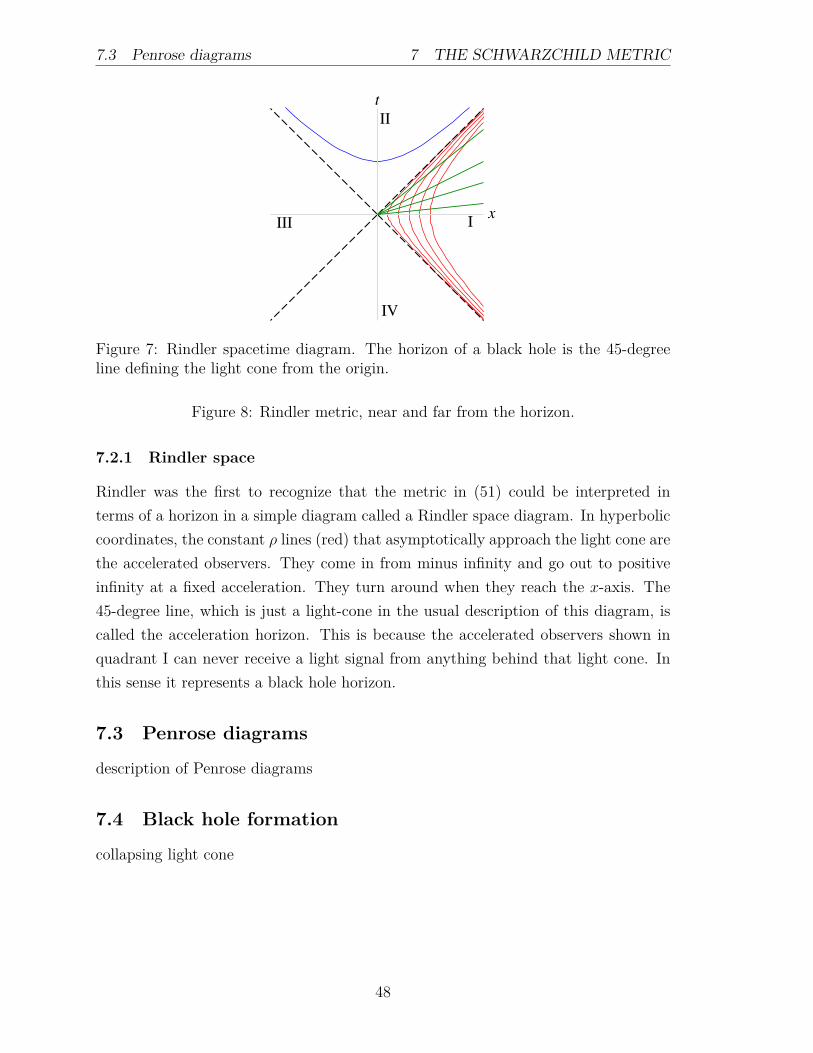
7.3 Penrose diagrams 7 THE SCHWARZCHILD METRIC

x

t

I

II

III

IV

Figure 7: Rindler spacetime diagram. The horizon of a black hole is the 45-degreeline defining the light cone from the origin.

Figure 8: Rindler metric, near and far from the horizon.

7.2.1 Rindler space

Rindler was the first to recognize that the metric in (51) could be interpreted interms of a horizon in a simple diagram called a Rindler space diagram. In hyperboliccoordinates, the constant ρ lines (red) that asymptotically approach the light cone arethe accelerated observers. They come in from minus infinity and go out to positiveinfinity at a fixed acceleration. They turn around when they reach the x-axis. The45-degree line, which is just a light-cone in the usual description of this diagram, iscalled the acceleration horizon. This is because the accelerated observers shown inquadrant I can never receive a light signal from anything behind that light cone. Inthis sense it represents a black hole horizon.

7.3 Penrose diagrams

description of Penrose diagrams

7.4 Black hole formation

collapsing light cone

48

7 THE SCHWARZCHILD METRIC 7.5 Counting black hole microstates

7.5 Counting black hole microstates

The following is a simplified argument for obtaining the entropy of a black hole fromstring theory. In units where c = h = 1 we have, dimensionally, length = time andenergy = 1/time, respectively. In particular this means that energy ~ 1/length, whichwe know from simple formulas like E = hc/λ for the energy of a photon of wavelengthλ. Newton’s constant in natural units is then [G] = [Fr2/M2] = El/E2 = l2 or unitsof length squared. This is the Planck length, so we write G ∼ l2P . In black holephysics or GR physics, the Beckenstein entropy formula is

SBH ∼ A/l2P = A/G, (54)

with A the area of the horizon. We would like to obtain this formula from stringyarguments. If the string coupling constant is g and this constant gives the amplitudefor a string to “emit” a closed loop (graviton) for absorption by another string, thenthe probability of a graviton exchange will be g4. The amplitude for the exchangeprocess is g2 because there are to events. If this is related to gravity we should beable to connect these ideas by writing g2 ∼ G but g is dimensionless. The only thingit can be related to with dimension is the characteristic string length, lS, which is thelength of the wiggles on a ball of string, not the size of the ball of string. Then wecan write

g2l2S = l2P (55)

or just glS = lP . This should make some sense in that the coupling constant shouldbe less than one, and we have g = lP/lS and lS > lP .

We now need the entropy of a string, or approximate entropy of a string. Theeasiest way to approximate it is to consider a simple cubic lattice of points that makeup space. The string can be any configuration from one point on the lattice to anotherand can even go back on itself. Then in one space dimension the string can move oneof two ways from each point. In two space dimensions, the string can move in any oneof four directions. Clearly in d dimensions the string can go in any of 2d directions. Ifthe string length is L = lSn, n links long, then the number of configurations is (2d)n.This gives an entropy for the string of SS = ln (2d)n = n ln 2d. This is essentiallySS ∼ n and from the string length equation we have

SS ∼ n = L/lS. (56)

Note the similarity with the Beckenstein formula, the characteristic parameter for a

49

7.5 Counting black hole microstates 7 THE SCHWARZCHILD METRIC

black hole is the area of the horizon, while for a string it is the string length. Simplydivide out the characteristic lengths to obtain a dimensionless quantity and we arriveat the entropy.

The entropy of the black hole can be written SBH = M2G2/G = M2G using theSchwarzchild radius RS ∼ MG. Can we write the string entropy in this way? Themass of the string is MS = n/lS where the mass of a segment of the string is 1/lS.Then we can write MS = L/l2S, and the entropy of the string as SS = L/lS = lSMS.Using (55) and G = l2Pwe can write SS = msMSG.

50