Ž . Coastal Engineering 41 2000 317–352 www.elsevier.comrlocatercoastaleng Suspended sediment modelling in a shelf sea ž / North Sea Herman Gerritsen a, ) , Robert J. Vos a,1 , Theo van der Kaaij a , Andrew Lane b , Johan G. Boon a a WL r Delft Hydraulics, P.O. Box 177, 2600 MH Delft, Netherlands b Proudman Oceanographic Laboratory, Bidston ObserÕatory, Birkenhead, CH43 7RA, UK Abstract Ž . This paper extends the modelling of suspended particulate matter SPM on the local coastal Ž . scale described in preceding papers to SPM modelling on the scale of the North Sea, focusing on representing SPM patterns and their seasonal distribution. The modelling includes a sensitivity study, in which model results are assessed using surface SPM concentration patterns extracted from NOAA reflectance imagery, as well as North Sea Project in situ data. Over the past decade or so, first-order estimates of the net suspended load and its associated sources and sinks have been available and are generally substantiated. However, developments in the simulation of large-scale SPM behaviour are still severely restricted by the available descriptions of available sediment sources and sediment erosion and deposition processes. This paper indicates how remotely sensed reflectance images can provide additional information on the Ž . spatial distribution of sea surface suspended sediments. A primary objective of this paper is to examine sensitivities of SPM simulations in 2D Ž . vertically averaged and 3D models. A boundary-fitted coordinate modelling approach with intra-tidal resolution and synoptic meteorology is applied, as well as more schematic approaches. A related objective is to examine how both limited in situ observational data and reflectance imagery can be used to assess and improve such simulations. Ž . An integrated modelling-monitoring approach, using inverse and ‘Goodness-of-Fit’ GoF approaches applied to remotely sensed reflectance imagery, is used to derive a structured sensitivity analysis providing a quantified assessment of the strengths and weaknesses of mod- elling and input data. It is shown that, especially in the coastal zone where salinity stratification ) Corresponding author. Tel.: q 31-15-2858470; fax: q 31-15-285-8582. Ž . E-mail address: [email protected] H. Gerritsen . 1 Present address: University of Amsterdam, Institute for Environmental Studies, de Boelelaan 1105, 1081 HV Amsterdam, Netherlands. 0378-3839r00r$ - see front matter q 2000 Elsevier Science B.V. All rights reserved. Ž . PII: S0378-3839 00 00042-9

Welcome message from author
This document is posted to help you gain knowledge. Please leave a comment to let me know what you think about it! Share it to your friends and learn new things together.
Transcript
Ž .Coastal Engineering 41 2000 317–352www.elsevier.comrlocatercoastaleng
Suspended sediment modelling in a shelf seaž /North Sea
Herman Gerritsen a,), Robert J. Vos a,1, Theo van der Kaaij a,Andrew Lane b, Johan G. Boon a
a WLrDelft Hydraulics, P.O. Box 177, 2600 MH Delft, Netherlandsb Proudman Oceanographic Laboratory, Bidston ObserÕatory, Birkenhead, CH43 7RA, UK
Abstract
Ž .This paper extends the modelling of suspended particulate matter SPM on the local coastalŽ .scale described in preceding papers to SPM modelling on the scale of the North Sea, focusing on
representing SPM patterns and their seasonal distribution. The modelling includes a sensitivitystudy, in which model results are assessed using surface SPM concentration patterns extractedfrom NOAA reflectance imagery, as well as North Sea Project in situ data.
Over the past decade or so, first-order estimates of the net suspended load and its associatedsources and sinks have been available and are generally substantiated. However, developments inthe simulation of large-scale SPM behaviour are still severely restricted by the availabledescriptions of available sediment sources and sediment erosion and deposition processes. Thispaper indicates how remotely sensed reflectance images can provide additional information on the
Ž .spatial distribution of sea surface suspended sediments.A primary objective of this paper is to examine sensitivities of SPM simulations in 2D
Ž .vertically averaged and 3D models. A boundary-fitted coordinate modelling approach withintra-tidal resolution and synoptic meteorology is applied, as well as more schematic approaches.A related objective is to examine how both limited in situ observational data and reflectanceimagery can be used to assess and improve such simulations.
Ž .An integrated modelling-monitoring approach, using inverse and ‘Goodness-of-Fit’ GoFapproaches applied to remotely sensed reflectance imagery, is used to derive a structuredsensitivity analysis providing a quantified assessment of the strengths and weaknesses of mod-elling and input data. It is shown that, especially in the coastal zone where salinity stratification
) Corresponding author. Tel.: q31-15-2858470; fax: q31-15-285-8582.Ž .E-mail address: [email protected] H. Gerritsen .
1 Present address: University of Amsterdam, Institute for Environmental Studies, de Boelelaan 1105, 1081HV Amsterdam, Netherlands.
0378-3839r00r$ - see front matter q2000 Elsevier Science B.V. All rights reserved.Ž .PII: S0378-3839 00 00042-9
( )H. Gerritsen et al.rCoastal Engineering 41 2000 317–352318
may occur, 3D modelling is required while much of the sensitivity analysis can be based on a 2Dmodelling approach. This quantification of the effects of uncertainties of inputs and erosionrde-position parameters improves understanding of the sediment distribution and budgets on the NorthSea scale.
It is concluded that whilst process studies are likely to contribute to improving erosionrdeposi-tion algorithms, and model developments will provide enhanced dynamical descriptions, accurate
Ž .overall simulation will remain dependent on some inverse processes to reduce the uncertainty insediment sources. q 2000 Elsevier Science B.V. All rights reserved.
Keywords: Boundary-fitted modelling grid; NOAArAVHRR reflectance imagery; Sensitivity analysis; Sus-pended sediment modelling; North Sea
1. Introduction
ŽA primary objective of PRe-Operational Modelling In the Seas of Europe PROM-.ISE was to develop the methodology to ‘quantify the rates and scales of exchange of
sediments between the coast and the near-shore zone’. This involves developing theŽ .capabilities to simulate near-shore waves Monbaliu et al., 2000 , couple these with
Ž . Žcurrents Ozer et al., 2000 and compute the resultant turbulence distributions Baumert.et al., 2000 . While these models provide the dynamical framework for the suspended
Ž .particulate matter SPM modelling, additional information on coastal and offshoreŽsources of sediments is required — direct monitoring by remote sensing Johannessen et
. Ž . Ž .al., 2000 or in situ observations Lane et al., 2000 provide by inverse means suchŽ .information. For eroding coasts, local area models Prandle et al., 2000 can provide
ŽSPM input to shelf sea scale simulations. For other coastal zones Schneggenburger et.al., 2000 , SPM exchanges may constitute alternatively imports and exports — differing
over seasons, tranquil or storm conditions and for fine-to-coarse sediments. In tidalŽ .straits Chapalain and Thais, 2000 , the exchange may be essentially a through-flow.
The primary objective of the modelling in this paper is the representation of thesuspended sediment distribution or patterns on the scale of the North Sea and theirvariation over the seasons. A related objective is to perform structured sensitivityanalyses to identify strengths and weaknesses of various approaches. The limitedmobility of coarse, sandy sediments restricts consideration here to finer siltrclayparticles, which can remain in suspension for periods of months. Both 2D and 3Dapproaches are considered. Tide resolving simulations with synoptic meteorology aremade, as well as simulations with spatially and temporally averaged hydrodynamics andforcing. A novel feature is the use of a boundary-fitted coordinate grid with highresolution in the coastal zones alongside modelling on a rectangular grid. For validationof the model results, both SPM in situ data sets and newly available remotely sensedreflectance imagery are used.
Summarising the above, we re-examine our knowledge of larger-scale SPM budgetsfor the North Sea, with the aim of identifying how modelling developments inPROMISE and more traditional in situ data sets plus newly available remotely sensed
Ž .data can be combined Vos et al., 2000 to advance this knowledge. In terms of the
( )H. Gerritsen et al.rCoastal Engineering 41 2000 317–352 319
Ž .scales of interest, the present work is comparable to the work by Lehmann et al. 1995 ,i.e. essentially North Sea wide, while most other North Sea applications consider a
Ž .small-scale local application see e.g. de Kok, 1992 .Section 2 comprises a review of existing sediment budget estimates for the North
Sea. Section 3 analyses the component modules required in a North Sea SPM model.Section 4 presents a 2D-model approach to determine the significance of sedimentsources for the SPM distribution in the North Sea, using multiple linear regressionŽ .McManus and Prandle, 1997 . Section 5 presents a sensitivity analysis of modelling ofthe North Sea SPM distribution and its seasonal distribution using a curvilinear grid in
Ž .2D and 3D and NOAA satellite reflectance imagery see also Gerritsen et al., 2000 . Inthe present analysis, attention is given to aspects such as uncertainties in hydrodynamics,forcing, etc., as well as SPM modelling per se.
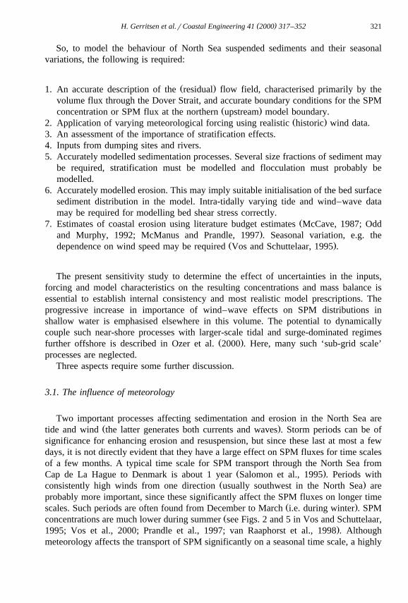
Reiterating — the aim in the modelling simulation is to reproduce the North Seascale SPM patterns and their seasonal variations — not individual localised, short-livedevents. Given the synoptic nature of remote sensing imagery, these data are better suitedfor validation than much of the in situ data. Fig. 1 gives a characteristic composite
Ž .Fig. 1. North Sea remote sensing reflectance image for March 1994 courtesy of KNMI . Note the plume ofsediment across the North Sea. The continental coast features a high concentration of sediment in a rathernarrow band of about 10–20 km.

( )H. Gerritsen et al.rCoastal Engineering 41 2000 317–352320
reflectance image of the North Sea, which is a measure for the SPM distribution at thesurface.
Conclusions and recommendations relating to future efforts follow in Section 6.
2. Estimation of North Sea SPM supplies and losses
ŽEstimates of supply and loss of sediment for the entire North Sea extending from the.Dover Strait to the Atlantic Ocean and the Baltic Sea , obtained from several references
in the literature are given in Appendix A, Tables A1 and A2. Many of these estimatesshow large uncertainties, and hence a detailed quantitative judgement may be misleadingŽ .Eisma and Irion, 1988 . Estimates are given here as an indication of sources and sinksof SPM in the North Sea.
The tables show that the most relevant sources of sediment in the North Sea are indecreasing order of importance:
Ø An influx of 20–40=109 kg yeary1 through the Dover StraitØ Effect of dumping from dredging activities, estimated to be 14=109 kg yeary1
Ø Influx from the Atlantic Ocean of 10=109 kg yeary1
Ž 9 y1.Ø Effect of coastal erosion from the east coast of England 2–8=10 kg yearŽ 9 y1.Ø River inputs 4=10 kg year
Estimates of sediment losses are:
9 y1 Ž 9 y1Ø Net sedimentation of 32–45=10 kg year of which 25=10 kg year outside.the model domain considered below
Ø Net outflow to the Atlantic Ocean of 11–14=109 kg yeary1
3. SPM modelling — component specifications
SPM is usually defined as the particles in suspension with a diameter smaller than 63Ž .mm but may include all particles that are in suspension. In the North Sea Project NSP
Ž .Natural Environment Research Council, 1992 , SPM was measured optically. In theNorth Sea, SPM determined with remote sensing usually corresponds to fine siltrclay,
Žsince only the top of the water column is sampled phytoplankton can generally be.differentiated in such data .
The SPM concentration is the result of the following three ‘processes’:
ŽØ Emissions of suspended matter river discharges, sewage sludge, dumping andŽ ..exchange with external waters inputs and boundary conditions
Ø Vertical transport and exchange with the seabed due to sedimentation and erosionprocesses, generated by currents and wind-induced waves
Ø Horizontal transport brought about by wind-, tide- and density-induced currents
( )H. Gerritsen et al.rCoastal Engineering 41 2000 317–352 321
So, to model the behaviour of North Sea suspended sediments and their seasonalvariations, the following is required:
Ž .1. An accurate description of the residual flow field, characterised primarily by thevolume flux through the Dover Strait, and accurate boundary conditions for the SPM
Ž .concentration or SPM flux at the northern upstream model boundary.Ž .2. Application of varying meteorological forcing using realistic historic wind data.
3. An assessment of the importance of stratification effects.4. Inputs from dumping sites and rivers.5. Accurately modelled sedimentation processes. Several size fractions of sediment may
be required, stratification must be modelled and flocculation must probably bemodelled.
6. Accurately modelled erosion. This may imply suitable initialisation of the bed surfacesediment distribution in the model. Intra-tidally varying tide and wind–wave datamay be required for modelling bed shear stress correctly.
Ž7. Estimates of coastal erosion using literature budget estimates McCave, 1987; Odd.and Murphy, 1992; McManus and Prandle, 1997 . Seasonal variation, e.g. the
Ž .dependence on wind speed may be required Vos and Schuttelaar, 1995 .
The present sensitivity study to determine the effect of uncertainties in the inputs,forcing and model characteristics on the resulting concentrations and mass balance isessential to establish internal consistency and most realistic model prescriptions. Theprogressive increase in importance of wind–wave effects on SPM distributions inshallow water is emphasised elsewhere in this volume. The potential to dynamicallycouple such near-shore processes with larger-scale tidal and surge-dominated regimes
Ž .further offshore is described in Ozer et al. 2000 . Here, many such ‘sub-grid scale’processes are neglected.
Three aspects require some further discussion.
3.1. The influence of meteorology
Two important processes affecting sedimentation and erosion in the North Sea areŽ .tide and wind the latter generates both currents and waves . Storm periods can be of
significance for enhancing erosion and resuspension, but since these last at most a fewdays, it is not directly evident that they have a large effect on SPM fluxes for time scalesof a few months. A typical time scale for SPM transport through the North Sea from
Ž .Cap de La Hague to Denmark is about 1 year Salomon et al., 1995 . Periods withŽ .consistently high winds from one direction usually southwest in the North Sea are
probably more important, since these significantly affect the SPM fluxes on longer timeŽ .scales. Such periods are often found from December to March i.e. during winter . SPM
Žconcentrations are much lower during summer see Figs. 2 and 5 in Vos and Schuttelaar,.1995; Vos et al., 2000; Prandle et al., 1997; van Raaphorst et al., 1998 . Although
meteorology affects the transport of SPM significantly on a seasonal time scale, a highly
( )H. Gerritsen et al.rCoastal Engineering 41 2000 317–352322
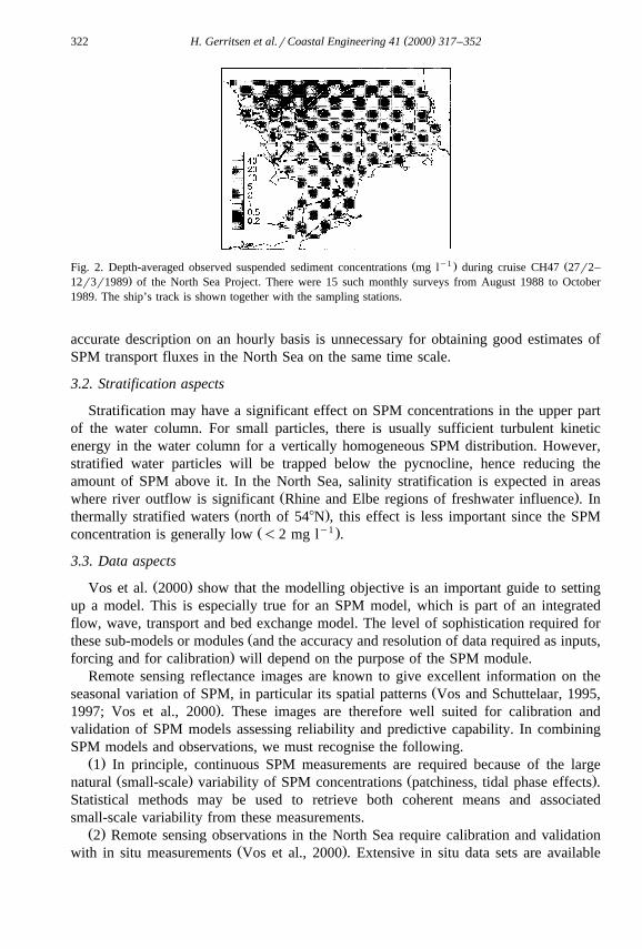
Ž y1 . ŽFig. 2. Depth-averaged observed suspended sediment concentrations mg l during cruise CH47 27r2–.12r3r1989 of the North Sea Project. There were 15 such monthly surveys from August 1988 to October
1989. The ship’s track is shown together with the sampling stations.
accurate description on an hourly basis is unnecessary for obtaining good estimates ofSPM transport fluxes in the North Sea on the same time scale.
3.2. Stratification aspects
Stratification may have a significant effect on SPM concentrations in the upper partof the water column. For small particles, there is usually sufficient turbulent kineticenergy in the water column for a vertically homogeneous SPM distribution. However,stratified water particles will be trapped below the pycnocline, hence reducing theamount of SPM above it. In the North Sea, salinity stratification is expected in areas
Ž .where river outflow is significant Rhine and Elbe regions of freshwater influence . InŽ .thermally stratified waters north of 548N , this effect is less important since the SPM
Ž y1 .concentration is generally low -2 mg l .
3.3. Data aspects
Ž .Vos et al. 2000 show that the modelling objective is an important guide to settingup a model. This is especially true for an SPM model, which is part of an integratedflow, wave, transport and bed exchange model. The level of sophistication required for
Žthese sub-models or modules and the accuracy and resolution of data required as inputs,.forcing and for calibration will depend on the purpose of the SPM module.
Remote sensing reflectance images are known to give excellent information on theŽseasonal variation of SPM, in particular its spatial patterns Vos and Schuttelaar, 1995,
.1997; Vos et al., 2000 . These images are therefore well suited for calibration andvalidation of SPM models assessing reliability and predictive capability. In combiningSPM models and observations, we must recognise the following.
Ž .1 In principle, continuous SPM measurements are required because of the largeŽ . Ž .natural small-scale variability of SPM concentrations patchiness, tidal phase effects .
Statistical methods may be used to retrieve both coherent means and associatedsmall-scale variability from these measurements.
Ž .2 Remote sensing observations in the North Sea require calibration and validationŽ .with in situ measurements Vos et al., 2000 . Extensive in situ data sets are available
( )H. Gerritsen et al.rCoastal Engineering 41 2000 317–352 323
Ž . Žfrom ZISCH Sundermann, 1994 and from the NSP Natural Environment Research¨.Council, 1992 . Large spatial coverage of the North Sea is obtained from remote sensing
data, notably NOAArAVHRR, for which high-quality processed data sets of weeklyand monthly composite images exist.
Ž .3 Knowledge of North Sea bed–sediment characteristics is varied. Information isŽ . Ž . Žfound in the studies by Jarke 1956 and van Alphen 1987 , from maps for example,
Figge, 1981; Geological Survey of The Netherlands, 1986; Balson et al., 1991; BritishŽ .. ŽGeological Survey BGS and from the recent Holderness Coastal Experiment Prandle
.et al., 2000 . Since the source of sediment at the seabed may have a large naturalvariability, accurate quantification of erosion fluxes is not possible.
Ž .4 The sophistication of SPM models is effectively limited by the amount of usefulfield data available to validate associated coefficients. Thus, the models here use onlythe simpler SPM concepts, usually having some four to six empirical parameters.
( )4. 2D SPM model rectangular coordinates
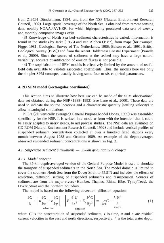
This section aims to illustrate how best use can be made of the SPM observationalŽ . Ž .data set obtained during the NSP 1988–1992 see Lane et al., 2000 . These data are
Ž .used to indicate the source locations and a characteristic quantity settling velocity toallow meaningful simulations.
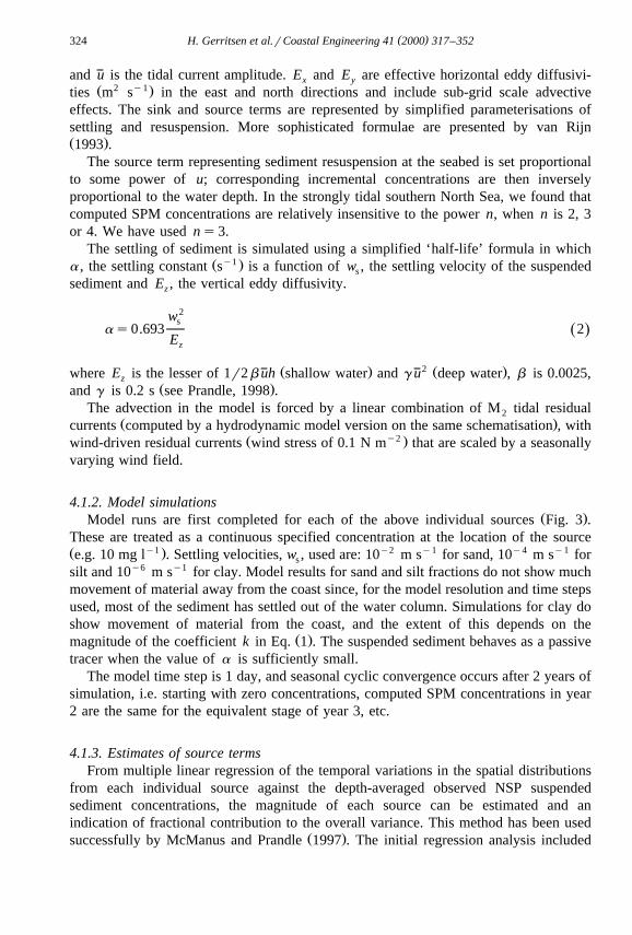
Ž . Ž .POL’s 2D vertically averaged General Purpose Model Jones, 1999 was assembledspecifically for the NSP. It is written in a modular form with the intention that it couldbe easily adapted to users’ needs, to aid process studies. The NSP data are available on
Ž .CD ROM Natural Environment Research Council, 1992 and include vertical profiles ofsuspended sediment concentration collected at over a hundred fixed stations everymonth between August 1988 and October 1989. An example of the depth-averagedobserved suspended sediment concentrations is shown in Fig. 2.
4.1. Suspended sediment simulations — 35-km grid, tidally aÕeraged
4.1.1. Model conceptThe 35-km depth-averaged version of the General Purpose Model is used to simulate
the transport of suspended sediments in the North Sea. The model domain is limited tocover the southern North Sea from the Dover Strait to 55.58N and includes the effects ofadvection, diffusion, settling of suspended sediments and resuspension. Sources of
Ž .sediment are from the major rivers Humber, Thames, Rhine, Elbe, TynerTees , theDover Strait and the northern boundary.
The model is based on the following advection–diffusion equation:n2 2 < <EC EC EC E C E C k u
q u qÕ y E qE sya Cq 1Ž .x y2 2Et Ex E y hEx E y sinksourceadvection diffusion
where C is the concentration of suspended sediment, t is time, u and Õ are residualcurrent velocities in the east and north directions, respectively, h is the total water depth,
( )H. Gerritsen et al.rCoastal Engineering 41 2000 317–352324
and u is the tidal current amplitude. E and E are effective horizontal eddy diffusivi-x yŽ 2 y1.ties m s in the east and north directions and include sub-grid scale advective
effects. The sink and source terms are represented by simplified parameterisations ofsettling and resuspension. More sophisticated formulae are presented by van RijnŽ .1993 .
The source term representing sediment resuspension at the seabed is set proportionalto some power of u; corresponding incremental concentrations are then inverselyproportional to the water depth. In the strongly tidal southern North Sea, we found thatcomputed SPM concentrations are relatively insensitive to the power n, when n is 2, 3or 4. We have used ns3.
The settling of sediment is simulated using a simplified ‘half-life’ formula in whichŽ y1 .a , the settling constant s is a function of w , the settling velocity of the suspendeds
sediment and E , the vertical eddy diffusivity.z
w2s
as0.693 2Ž .Ez
2Ž . Ž .where E is the lesser of 1r2b uh shallow water and g u deep water , b is 0.0025,zŽ .and g is 0.2 s see Prandle, 1998 .
The advection in the model is forced by a linear combination of M tidal residual2Ž .currents computed by a hydrodynamic model version on the same schematisation , with
Ž y2 .wind-driven residual currents wind stress of 0.1 N m that are scaled by a seasonallyvarying wind field.
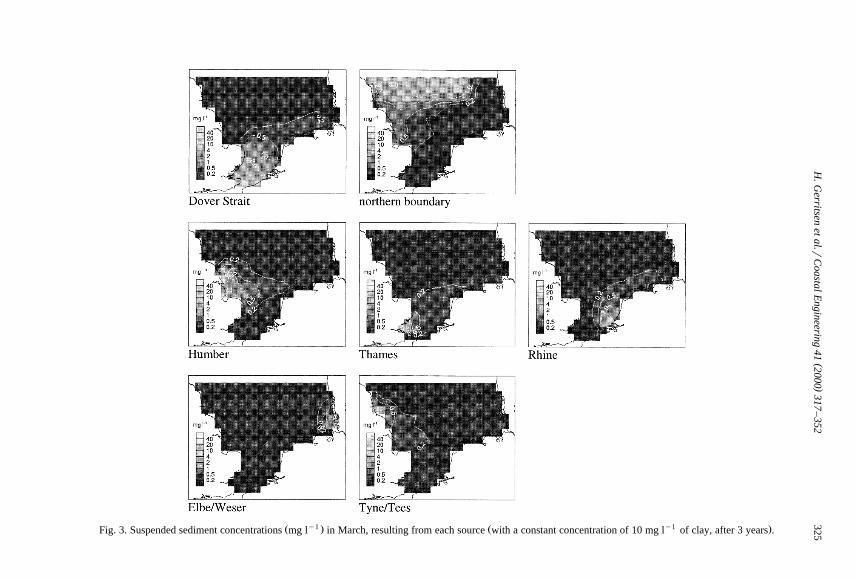
4.1.2. Model simulationsŽ .Model runs are first completed for each of the above individual sources Fig. 3 .
These are treated as a continuous specified concentration at the location of the sourceŽ y1 . y2 y1 y4 y1e.g. 10 mg l . Settling velocities, w , used are: 10 m s for sand, 10 m s fors
silt and 10y6 m sy1 for clay. Model results for sand and silt fractions do not show muchmovement of material away from the coast since, for the model resolution and time stepsused, most of the sediment has settled out of the water column. Simulations for clay doshow movement of material from the coast, and the extent of this depends on the
Ž .magnitude of the coefficient k in Eq. 1 . The suspended sediment behaves as a passivetracer when the value of a is sufficiently small.
The model time step is 1 day, and seasonal cyclic convergence occurs after 2 years ofsimulation, i.e. starting with zero concentrations, computed SPM concentrations in year2 are the same for the equivalent stage of year 3, etc.
4.1.3. Estimates of source termsFrom multiple linear regression of the temporal variations in the spatial distributions
from each individual source against the depth-averaged observed NSP suspendedsediment concentrations, the magnitude of each source can be estimated and anindication of fractional contribution to the overall variance. This method has been used
Ž .successfully by McManus and Prandle 1997 . The initial regression analysis included
()
H.G
erritsenet
al.rC
oastalEngineering
412000
317–
352325Ž y1 . Ž y1 .Fig. 3. Suspended sediment concentrations mg l in March, resulting from each source with a constant concentration of 10 mg l of clay, after 3 years .
( )H. Gerritsen et al.rCoastal Engineering 41 2000 317–352326
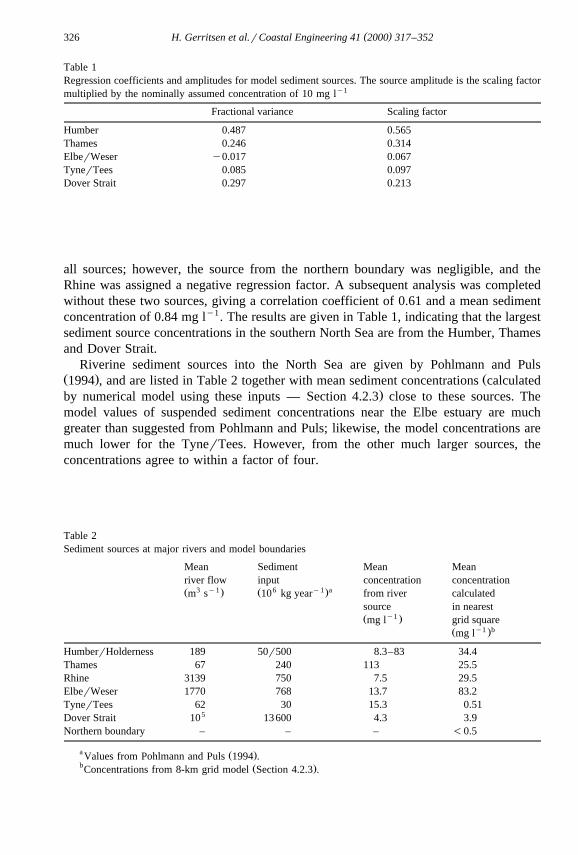
Table 1Regression coefficients and amplitudes for model sediment sources. The source amplitude is the scaling factormultiplied by the nominally assumed concentration of 10 mg ly1
Fractional variance Scaling factor
Humber 0.487 0.565Thames 0.246 0.314ElberWeser y0.017 0.067TynerTees 0.085 0.097Dover Strait 0.297 0.213
all sources; however, the source from the northern boundary was negligible, and theRhine was assigned a negative regression factor. A subsequent analysis was completedwithout these two sources, giving a correlation coefficient of 0.61 and a mean sedimentconcentration of 0.84 mg ly1. The results are given in Table 1, indicating that the largestsediment source concentrations in the southern North Sea are from the Humber, Thamesand Dover Strait.
Riverine sediment sources into the North Sea are given by Pohlmann and PulsŽ . Ž1994 , and are listed in Table 2 together with mean sediment concentrations calculated
.by numerical model using these inputs — Section 4.2.3 close to these sources. Themodel values of suspended sediment concentrations near the Elbe estuary are muchgreater than suggested from Pohlmann and Puls; likewise, the model concentrations aremuch lower for the TynerTees. However, from the other much larger sources, theconcentrations agree to within a factor of four.
Table 2Sediment sources at major rivers and model boundaries
Mean Sediment Mean Meanriver flow input concentration concentration
3 y1 6 y1 aŽ . Ž .m s 10 kg year from river calculatedsource in nearest
y1Ž .mg l grid squarey1 bŽ .mg l
HumberrHolderness 189 50r500 8.3–83 34.4Thames 67 240 113 25.5Rhine 3139 750 7.5 29.5ElberWeser 1770 768 13.7 83.2TynerTees 62 30 15.3 0.51
5Dover Strait 10 13600 4.3 3.9Northern boundary – – – -0.5
a Ž .Values from Pohlmann and Puls 1994 .b Ž .Concentrations from 8-km grid model Section 4.2.3 .
( )H. Gerritsen et al.rCoastal Engineering 41 2000 317–352 327
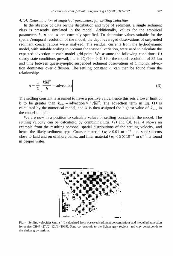
4.1.4. Determination of empirical parameters for settling ÕelocitiesIn the absence of data on the distribution and type of sediment, a single sediment
class is presently simulated in the model. Additionally, values for the empiricalparameters k, n and a are currently specified. To determine values suitable for thespatialrtemporal resolution of the model, the depth-averaged observations of suspendedsediment concentrations were analysed. The residual currents from the hydrodynamicmodel, with suitable scaling to account for seasonal variation, were used to calculate the
Ž .expected advection at each model grid-point. We assume the following conditions: iŽ .steady-state conditions prevail, i.e. is ECrEts0, ii for the model resolution of 35 km
and time between quasi-synoptic suspended sediment observations of 1 month, advec-tion dominates over diffusion. The settling constant a can then be found from therelationship:
n< <1 k uas yadvection 3Ž .
C h
The settling constant is assumed to have a positive value, hence this sets a lower limit ofn< < Ž .k to be greater than k sadvection=hr u . The advection term in Eq. 1 ismin
calculated by the numerical model, and k is then assigned the highest value of k inmin
the model domain.We are now in a position to calculate values of settling constant in the model. The
Ž . Ž .settling velocity can be calculated by combining Eqs. 2 and 3 . Fig. 4 shows anexample from the resulting seasonal spatial distributions of the settling velocity, and
Ž y1 .hence the likely sediment type. Coarser material w )0.01 m s , i.e. sand occurssŽ y4 y1.close to land and on offshore banks, and finer material w -5=10 m s is founds
in deeper water.
Ž y1 .Fig. 4. Settling velocities mm s calculated from observed sediment concentrations and modelled advectionŽ .for cruise CH47 27r2–12r3r1989 . Sand corresponds to the lighter grey regions, and clay corresponds to
the darker grey regions.
( )H. Gerritsen et al.rCoastal Engineering 41 2000 317–352328
4.2. Suspended sediment simulations — 8-km grid, tidally resolÕing
4.2.1. Model conceptThe 35-km model grid spacing is too large to resolve the shallow coastal regions, and
is also insufficient for sediment sources to be identified accurately. A higher resolutionmodel was therefore required.
An 8-km version of the General Purpose Model was employed to carry out thesuspended sediment simulation. The S tidal residual transports are included, in addition2
to M residuals and monthly varying wind-driven residuals. The model time-step is 152
min.The sediment sources are again at rivers and the model open boundaries. This time,
the model resolution is sufficiently fine so that the river sources can be specified as massŽ .input rates given in Table 2 .
4.2.2. Sedimentation and erosionŽ .In addition to the sourcersink terms from Eq. 1 , simulations were also made using
Ž Ž . Ž ..‘threshold stress’ formulae Eqs. 4 and 5 to represent the deposition and erosionŽ .processes from Odd and Murphy, 1992; Krone–Partheniades formulae .
t d tbdC s 1y C w for t -t otherwise dC s0 4Ž .dep bed s b dep dep
t hdep
t d tbdC s y1 E for t )t otherwise dC s0 5Ž .ero 0 b ero ero
t hero
where C is the suspended sediment concentration close to the seabed, t is the stressbed b
at the seabed. The threshold stress for deposition, t , is assumed equal to that fordep
erosion, t , with a value of 0.06 N my2 . The erosion rate E is 0.1 kg my2 sy1. Toero 0
simplify the calculations, we assume in this case that there is an unlimited supply ofsediment at the seabed for resuspension and keep track of the amount of material insuspension as well as on the seabed.
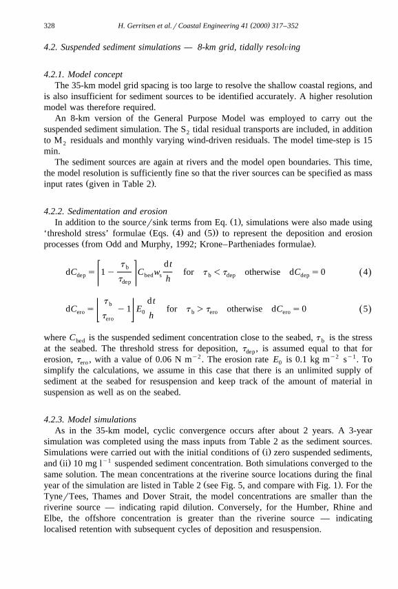
4.2.3. Model simulationsAs in the 35-km model, cyclic convergence occurs after about 2 years. A 3-year
simulation was completed using the mass inputs from Table 2 as the sediment sources.Ž .Simulations were carried out with the initial conditions of i zero suspended sediments,
Ž . y1and ii 10 mg l suspended sediment concentration. Both simulations converged to thesame solution. The mean concentrations at the riverine source locations during the final
Ž .year of the simulation are listed in Table 2 see Fig. 5, and compare with Fig. 1 . For theTynerTees, Thames and Dover Strait, the model concentrations are smaller than theriverine source — indicating rapid dilution. Conversely, for the Humber, Rhine andElbe, the offshore concentration is greater than the riverine source — indicatinglocalised retention with subsequent cycles of deposition and resuspension.
( )H. Gerritsen et al.rCoastal Engineering 41 2000 317–352 329
Fig. 5. Depth-averaged suspended sediment concentrations predicted by the 8-km grid model in March of yearŽ .3, resulting from the clay sources given in Table 2.
Ž .Direct comparison with observations is complicated by i availability and poorŽ .timerspace resolution of direct observations, ii sharp gradients of suspended sediment
concentrations close to the sources. It is therefore more realistic to compare, instead,patterns in the model results with that of observations rather than the absolute valuesŽ .see for example, the curvilinear approach in Section 5 .
( )5. 3D and 2D SPM model curvilinear grid
In this section, a sensitivity analysis of the modelling of North Sea SPM distributionand its seasonal distribution is presented. A curvilinear grid in 2D and 3D is used
Žtogether with NOAA satellite reflectances in the assessment Boon et al., 1997;.Gerritsen et al., 2000 . We first discuss the specific model set-up and key model aspects
such as the net hydrodynamic volume transport, the inclusion of wind–wave effects inthe SPM model, the formulation of settling, erosion and sedimentation processes in 2Dand 3D, and the effect of stratification. In subsequent subsections, the sensitivity
Ž .analysis for the 2D model application and the 3D model application on the same gridare discussed.
It is noted once again that the aim in the modelling simulation is to reproduce theNorth Sea scale SPM patterns and their seasonal variations — not individual localised,short-lived events. With its synoptic nature, remote sensing image data are more suitedfor validation than much of the in situ data. The focus is on using NOAArAVHRRimages for SPM, while using a structured modelling approach to assess results and
Ž .sensitivities see also Vos et al., 2000 .Modelling SPM correctly on a seasonal scale requires a chain of models or modules
forming an integrated model. This sequence is outlined below.Ø A hydrodynamic model for tidally and meteorologically induced flows, with
inclusion of salinity variation and a model for the turbulence parameters. The modeldomain, model grid and related gridded model geometry and bathymetry should be
( )H. Gerritsen et al.rCoastal Engineering 41 2000 317–352330
designed to reflect the requirements of the SPM transports, rather than the hydrodynam-ics per se.
Ø A wave module to generate wave characteristics that are key parameters in bederosion. Here, the wave-induced bed shear stress is the relevant parameter rather thanaccurate wave spectra.
Ø The SPM transport model based on the hydrodynamic database, to which is linkeda module describing the sedimentation and erosion processes and flocculation of silt.
There are uncertainties associated with each module and the resulting errors propa-Ž .gate from one module to the next see Fig. 1 of Vos et al., 2000 . To make an
assessment of the SPM modelling, we need to qualitatively analyse the uncertainties dueŽ .to: specification of bathymetry, hydrodynamics effect on residual flow , meteorological
Ž .forcing fixed wind or spatially and temporally varying wind , wind–waves andstratification and inputs such as dumping and coastal erosion.
The uncertainties due to parameter variations of the SPM model are quantified andŽ . Ž .ranked employing a ‘Goodness-of-Fit’ GoF concept outlined by Vos et al. 2000 or, inŽ .more detail by ten Brummelhuis et al. 2000 .
5.1. Model set-up and hydrodynamics
The model area and model grid were selected by taking into account the objectives ofthis modelling, i.e. accurate simulation of the large-scale spatial behaviour of suspendedmatter in the region. Given the importance of sediment fluxes through the Dover Strait,the model domain was extended into the English Channel. The grid was designed toreflect the requirements of all processes in the integrated model, which led to the
Ž .following grid characteristics: 1 an orthogonal curvilinear boundary fitted grid designthat is sufficiently detailed and smooth in the Dover Strait to represent the local flows
Ž .and sediment transport; 2 a grid design that allows for a proper numerical representa-tion of the strong cross-shore SPM gradients in the near-coastal zone. Attention has beengiven to the interfacing with an encompassing model in view of meteorological forcing,in order to analyse the sensitivity to propagation of uncertainties and errors in such
Ž .linking; 3 highest resolution in the near-coastal zone where most of the sedimentŽ . Žtransport and processes take place; and 4 a s-coordinate approach for the 3D
.simulations to ensure sufficient vertical resolution in the near-coastal zone.In view of computational flexibility, the number of horizontal computational elements
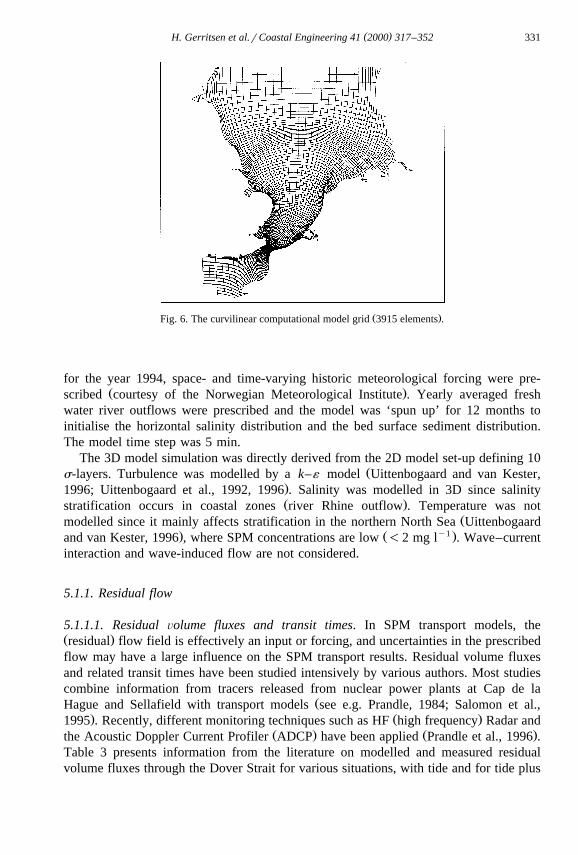
is limited in the central parts of the model area. The resulting model grid is shown inFig. 6.
The hydrodynamic basis of the suspended matter modelling is created by applying thehydrostatic inhomogeneous tide resolving 2D and 3D shallow water equations including
Ž .a k–´ turbulence model on a general orthogonal curvilinear grid Delft3D, 1997 . Thegridded bathymetry with varying detail was constructed merging available model
Ž .bathymetries of North Sea Model Advection Dispersion Study NOMADS andŽPROMISE partners. The bathymetry and open boundary tidal forcing obtained byŽ .nesting the model in the shelf-wide model Dutch Continental Shelf Model DCSM were
adjusted by applying adjoint modelling techniques and water level criteria, using theŽ .model in 2D mode ten Brummelhuis et al., 1997 . In the historic hindcast simulations
( )H. Gerritsen et al.rCoastal Engineering 41 2000 317–352 331
Ž .Fig. 6. The curvilinear computational model grid 3915 elements .
for the year 1994, space- and time-varying historic meteorological forcing were pre-Ž .scribed courtesy of the Norwegian Meteorological Institute . Yearly averaged fresh
water river outflows were prescribed and the model was ‘spun up’ for 12 months toinitialise the horizontal salinity distribution and the bed surface sediment distribution.The model time step was 5 min.
The 3D model simulation was directly derived from the 2D model set-up defining 10Žs-layers. Turbulence was modelled by a k–´ model Uittenbogaard and van Kester,
.1996; Uittenbogaard et al., 1992, 1996 . Salinity was modelled in 3D since salinityŽ .stratification occurs in coastal zones river Rhine outflow . Temperature was not
Žmodelled since it mainly affects stratification in the northern North Sea Uittenbogaard. Ž y1 .and van Kester, 1996 , where SPM concentrations are low -2 mg l . Wave–current
interaction and wave-induced flow are not considered.
5.1.1. Residual flow
5.1.1.1. Residual Õolume fluxes and transit times. In SPM transport models, theŽ .residual flow field is effectively an input or forcing, and uncertainties in the prescribedflow may have a large influence on the SPM transport results. Residual volume fluxesand related transit times have been studied intensively by various authors. Most studiescombine information from tracers released from nuclear power plants at Cap de la
ŽHague and Sellafield with transport models see e.g. Prandle, 1984; Salomon et al.,. Ž .1995 . Recently, different monitoring techniques such as HF high frequency Radar and
Ž . Ž .the Acoustic Doppler Current Profiler ADCP have been applied Prandle et al., 1996 .Table 3 presents information from the literature on modelled and measured residualvolume fluxes through the Dover Strait for various situations, with tide and for tide plus
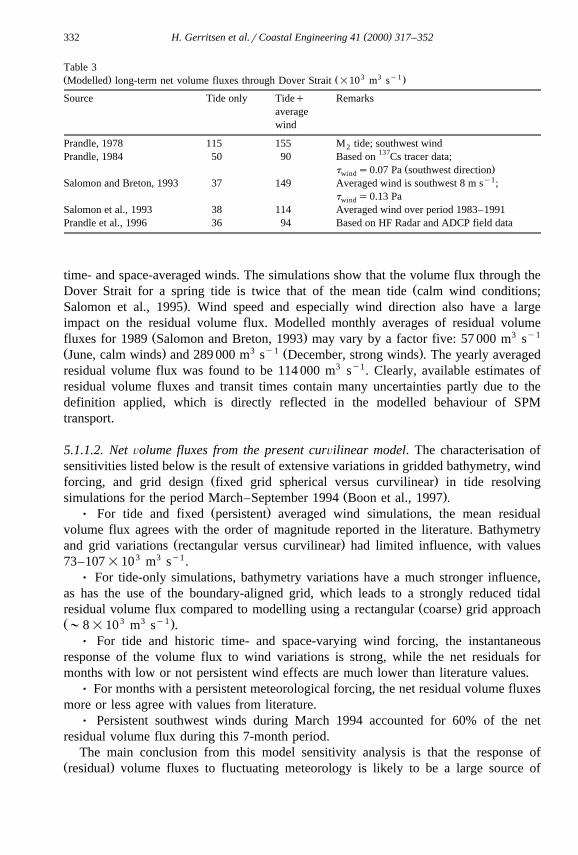
( )H. Gerritsen et al.rCoastal Engineering 41 2000 317–352332
Table 3Ž . Ž 3 3 y1.Modelled long-term net volume fluxes through Dover Strait =10 m s
Source Tide only Tideq Remarksaveragewind
Prandle, 1978 115 155 M tide; southwest wind2137Prandle, 1984 50 90 Based on Cs tracer data;
Ž .t s0.07 Pa southwest directionwindy1Salomon and Breton, 1993 37 149 Averaged wind is southwest 8 m s ;
t s0.13 Pawind
Salomon et al., 1993 38 114 Averaged wind over period 1983–1991Prandle et al., 1996 36 94 Based on HF Radar and ADCP field data
time- and space-averaged winds. The simulations show that the volume flux through theŽDover Strait for a spring tide is twice that of the mean tide calm wind conditions;
.Salomon et al., 1995 . Wind speed and especially wind direction also have a largeimpact on the residual volume flux. Modelled monthly averages of residual volume
Ž . 3 y1fluxes for 1989 Salomon and Breton, 1993 may vary by a factor five: 57 000 m sŽ . 3 y1 Ž .June, calm winds and 289 000 m s December, strong winds . The yearly averagedresidual volume flux was found to be 114 000 m3 sy1. Clearly, available estimates ofresidual volume fluxes and transit times contain many uncertainties partly due to thedefinition applied, which is directly reflected in the modelled behaviour of SPMtransport.
5.1.1.2. Net Õolume fluxes from the present curÕilinear model. The characterisation ofsensitivities listed below is the result of extensive variations in gridded bathymetry, wind
Ž .forcing, and grid design fixed grid spherical versus curvilinear in tide resolvingŽ .simulations for the period March–September 1994 Boon et al., 1997 .
Ž .Ø For tide and fixed persistent averaged wind simulations, the mean residualvolume flux agrees with the order of magnitude reported in the literature. Bathymetry
Ž .and grid variations rectangular versus curvilinear had limited influence, with values73–107=103 m3 sy1.
Ø For tide-only simulations, bathymetry variations have a much stronger influence,as has the use of the boundary-aligned grid, which leads to a strongly reduced tidal
Ž .residual volume flux compared to modelling using a rectangular coarse grid approachŽ 3 3 y1.;8=10 m s .
Ø For tide and historic time- and space-varying wind forcing, the instantaneousresponse of the volume flux to wind variations is strong, while the net residuals formonths with low or not persistent wind effects are much lower than literature values.
Ø For months with a persistent meteorological forcing, the net residual volume fluxesmore or less agree with values from literature.
Ø Persistent southwest winds during March 1994 accounted for 60% of the netresidual volume flux during this 7-month period.
The main conclusion from this model sensitivity analysis is that the response ofŽ .residual volume fluxes to fluctuating meteorology is likely to be a large source of
( )H. Gerritsen et al.rCoastal Engineering 41 2000 317–352 333
error. This suggests the need for a fundamental improvement of the air–sea momentumexchange concept for long-term flow modelling. Until then, the present common
Ž .approach of calibrating long-term volume fluxes using time-averaged persistent windŽ .estimates Salomon et al., 1995 is best practice.
5.1.1.3. Transit times of radionuclides discharged at Cap de la Hague. An estimatedmean persistent wind of 7 m sy1 from the southwest was used in a 2D model to
Ždetermine transit times of a tracer patch released from Cap de la Hague 1st March.1994 . This was compared with 2D model-based long-term transit time results calibrated
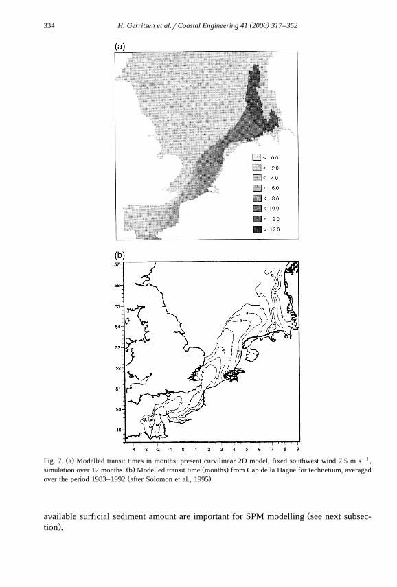
Ž .on experimental radionuclide data from Salomon et al. 1995 . The results are shown inFig. 7 and compare well. The model results also compare well with residual volume flux
Ž .estimates from HF Radar and ADCP by Prandle et al. 1996 , but deviate from these forhigh winds and very calm conditions.
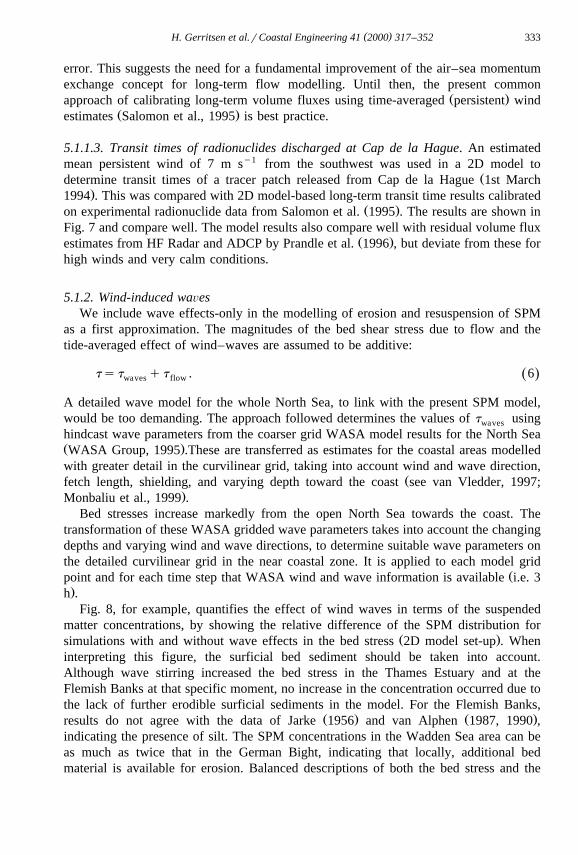
5.1.2. Wind-induced waÕesWe include wave effects-only in the modelling of erosion and resuspension of SPM
as a first approximation. The magnitudes of the bed shear stress due to flow and thetide-averaged effect of wind–waves are assumed to be additive:
tst qt . 6Ž .waves flow
A detailed wave model for the whole North Sea, to link with the present SPM model,would be too demanding. The approach followed determines the values of t usingwaves
hindcast wave parameters from the coarser grid WASA model results for the North SeaŽ .WASA Group, 1995 .These are transferred as estimates for the coastal areas modelledwith greater detail in the curvilinear grid, taking into account wind and wave direction,
Žfetch length, shielding, and varying depth toward the coast see van Vledder, 1997;.Monbaliu et al., 1999 .
Bed stresses increase markedly from the open North Sea towards the coast. Thetransformation of these WASA gridded wave parameters takes into account the changingdepths and varying wind and wave directions, to determine suitable wave parameters onthe detailed curvilinear grid in the near coastal zone. It is applied to each model grid
Žpoint and for each time step that WASA wind and wave information is available i.e. 3.h .
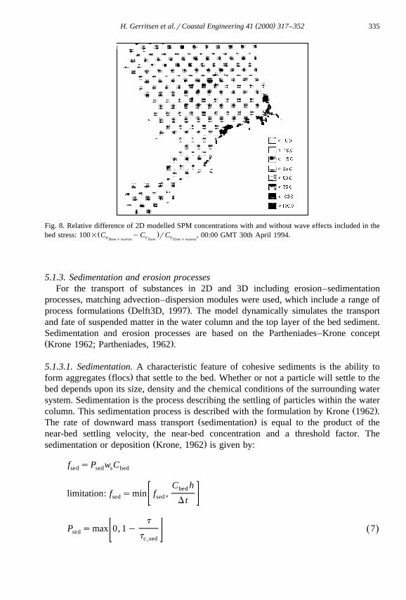
Fig. 8, for example, quantifies the effect of wind waves in terms of the suspendedmatter concentrations, by showing the relative difference of the SPM distribution for
Ž .simulations with and without wave effects in the bed stress 2D model set-up . Wheninterpreting this figure, the surficial bed sediment should be taken into account.Although wave stirring increased the bed stress in the Thames Estuary and at theFlemish Banks at that specific moment, no increase in the concentration occurred due tothe lack of further erodible surficial sediments in the model. For the Flemish Banks,
Ž . Ž .results do not agree with the data of Jarke 1956 and van Alphen 1987, 1990 ,indicating the presence of silt. The SPM concentrations in the Wadden Sea area can beas much as twice that in the German Bight, indicating that locally, additional bedmaterial is available for erosion. Balanced descriptions of both the bed stress and the
( )H. Gerritsen et al.rCoastal Engineering 41 2000 317–352334
Ž . y1Fig. 7. a Modelled transit times in months; present curvilinear 2D model, fixed southwest wind 7.5 m s ,Ž . Ž .simulation over 12 months. b Modelled transit time months from Cap de la Hague for technetium, averagedŽ .over the period 1983–1992 after Solomon et al., 1995 .
Žavailable surficial sediment amount are important for SPM modelling see next subsec-.tion .
( )H. Gerritsen et al.rCoastal Engineering 41 2000 317–352 335
Fig. 8. Relative difference of 2D modelled SPM concentrations with and without wave effects included in theŽ .bed stress: 100= C yC rC , 00:00 GMT 30th April 1994.t t tflowqwaves flow flowqwaves
5.1.3. Sedimentation and erosion processesFor the transport of substances in 2D and 3D including erosion–sedimentation
processes, matching advection–dispersion modules were used, which include a range ofŽ .process formulations Delft3D, 1997 . The model dynamically simulates the transport
and fate of suspended matter in the water column and the top layer of the bed sediment.Sedimentation and erosion processes are based on the Partheniades–Krone conceptŽ .Krone 1962; Partheniades, 1962 .
5.1.3.1. Sedimentation. A characteristic feature of cohesive sediments is the ability toŽ .form aggregates flocs that settle to the bed. Whether or not a particle will settle to the
bed depends upon its size, density and the chemical conditions of the surrounding watersystem. Sedimentation is the process describing the settling of particles within the water
Ž .column. This sedimentation process is described with the formulation by Krone 1962 .Ž .The rate of downward mass transport sedimentation is equal to the product of the
near-bed settling velocity, the near-bed concentration and a threshold factor. TheŽ .sedimentation or deposition Krone, 1962 is given by:
f sP w Csed sed s bed
C hbedlimitation: f smin f ,sed sed
D t
tP smax 0, 1y 7Ž .sed
tc ,sed
( )H. Gerritsen et al.rCoastal Engineering 41 2000 317–352336
Ž y2 y1. Ž .where f is the sedimentation flux of SPM kg m s , D t the model time step s ,sedŽ . Ž y1 .h the average water depth m , w the settling velocity of SPM m s , C thes bed
Ž y3 .concentration of SPM near the bed kg m , P the sedimentation factor, t the bedsedŽ . Ž . Ž .shear stress Pa and t the critical shear stress for sedimentation Pa . Eqs. 4 andc,sed
Ž .7 differ in that the latter formally assumes an upper limit to the sedimentation rate toavoid negative concentrations in the model.
5.1.3.2. Settling Õelocity w , 2D model. Various laboratory and field measurements shows
that the suspended matter concentration strongly influences the aggregation process andthereby the settling velocities of the aggregates. Large-size flocs are denser and havehigher settling velocities. In 2D, the effect of the sediment concentration on the
Žflocculation process can be described by the following common formula after van.Leussen, 1994 :
w slC m 8Ž .s
Ž y1 . Ž ymwhere w is the settling velocity m s , l the velocity conversion constant kgs3mq1 y1. Ž y3 .m s , and C the suspended matter concentration kg m .The settling velocity is not constant in time and space for values of m/0 used. In
Ž .the literature, m ranges from 0 to 2 van Leussen, 1994 . The spread in settlingvelocities increases with m. Therefore, for larger m, more size fractions of sediment areeffectively lumped into the single fraction model. In coastal areas where concentrationsand concentration gradients are high, large spatial differences in settling velocities areobtained with this approach. This mimics the presence of various fractions in theseareas.
5.1.3.3. Erosion. Erosion of seabed material occurs when the bed shear forces exceedthe resistance of the bed sediment. The resistance of the bed is characterised by a certaincritical erosive shear stress. This critical stress is determined by several factors, such as,the chemical composition of the bed material, particle size distribution and bioturbation.Since often only qualitative information on the type of bed is available, usually auniform value for this critical shear stress is employed in large-scale models. Erosion ofsediment is induced by the bed stress due to tidal and wind-induced advective flows andsurface waves.
Erosion is directly proportional to the excess of the applied shear stress over thecritical bed shear stress for erosion. The erosion of homogeneous beds is based on the
Ž .resuspension formula of Partheniades 1962 :
f sP Eres res 0
limitations: 1 f s0 if h-hŽ . res min
DM2 f smin f ,Ž . res res
D tA
tP smax 0, y1 9Ž .res
tc ,ero
( )H. Gerritsen et al.rCoastal Engineering 41 2000 317–352 337
Table 4Sedimentation characteristics
Parameter Value Reference
Ž .Critical stress for sedimentation t 0.04 Pa Nicholson and O’Connor, 1986c,sed
0.05–0.25 Pa Winterwerp, 19890.10–0.12 Pa Amos and Mosher, 1985
y1Ž .Settling velocity w 0.27–2.1 mm s Amos and Mosher, 1985sy10.01–0.1 mm s Mehta, 1986
Ž .Settling velocity constant l 0.513 Thorn, 1981 Severn EstuaryŽ .Settling velocity constant m 1.33 Krone, 1962 San Francisco BayŽ .1.29 Thorn, 1981 Severn Estuary
mŽ . Ž .w s lC 1.2 van Leussen, 1994 Ems EstuarysŽ .1.37 Burt, 1986 Thames Estuary
Ž .1.04 Puls et al., 1988 Elbe Estuary
Ž y2 y1.where f is the erosion rate kg m s , P the erosion threshold factor, E theres DW res 0Ž y2 y1. Ž .first-order erosion rate kg m s , t the bed shear stress Pa , t the criticalDW c,eroŽ . Ž .shear stress for erosion Pa , h the minimal water depth for erosion default 0.1 mmin
and DMrA the amount of locally available dry matter, expressed as dry weight per unitŽ y2 . Ž . Ž .square kg m . Eqs. 5 and 9 differ in that in the latter, the limitation by theDW
available erodible surface sediments is formally included.The value of E strongly depends on the sediment properties and environmental0
parameters. In this model, the erosion rate is limited by the available amount ofsediment, which has settled in previous periods.
A first estimate of suitable parameter values for North Sea sedimentation and erosionof suspended matter is obtained from laboratory and field experiments quoted inliterature. Tables 4 and 5 summarise some typical ranges of sedimentation and erosionparameter values found for estuaries and coastal zones.
The wide ranges found, sometimes factors of 10 or more, show that model parametersserve as bulk parameters in which different detailed processes are lumped. As argued
Ž .above and in more detail in Vos et al. 2000 , given the level of information in the data,we consider it unwarranted to model these processes with much more detail.
5.1.3.4. Settling Õelocity in 3D modelling. In 2D modelling, the water column isassumed to be always completely mixed, so the settling velocity w is verticallys
Table 5Erosion characteristics
Parameter Value Reference
Ž .Critical stress for erosion t 0.05–0.4 Pa Mehta et al., 1982c,ero
0.1–0.5 Pa Winterwerp, 1989y2Erosion rate E 0.01–0.5 g m s Winterwerp, 19890
y20.002–0.02 g m s Kappe et al., 1989
( )H. Gerritsen et al.rCoastal Engineering 41 2000 317–352338
uniform. In 3D modelling, the vertically varying settling velocity w in combinations
with the vertical diffusion coefficient given by the hydrodynamic k–´ module, deter-mines the sedimentation flux. Information from the literature on suitable w values fors
regional scales like the North Sea is limited, and most experimental information refers tosettling velocities for estuaries and coastal zones. The effect of vertical variation may be
Ž .illustrated on the analytic solution in one-dimensional vertical 1DV of the stationarytransport problem with vertical diffusion and concentration-dependent settling velocityand no net sedimentation or erosion.
y1rmlmz
ymC z s qC 10Ž . Ž .bedD
Ž . Ž .where z is the distance from the bed m , C the SPM concentration at the bed zs0bedŽ y3 . Ž 2 y1.kg m , D the vertical diffusion coefficient m s , m the power of concentration-
Ž . Ž ym 3mq1dependent settling m)0 , and l the velocity conversion constant 0.001 kg my1 .s .
This equation shows the basic concept for 3D: a steep decrease in concentration fromthe water surface to the seabed for finite vertical diffusivity with D-0.001 m2 sy1 forthe values of ls5.13=10y4 kgym m3mq1 sy1 and ms1.29 that were used. For the
Ž y2 2 y12D case, one must substitute an infinite value for D Ds1.0=10 m s readily. Žsuffices , and a well-mixed column results. In 3D, the settling velocity as a function of.l and m clearly has an effect for small diffusion, e.g. with stratification and concentra-
tion differences within the water column. Analogous to the 2D case, the settling velocitynear the bed will determine the sedimentation flux.
5.1.4. Stratification and turbulenceStratification may have an important effect on the vertical distribution of cohesive
sediment in the water column. Before embarking upon large-scale 2D and 3D simula-tions, a computationally simple but conceptually rather refined 1DV model was appliedto study the importance of temperature and salinity for the distribution of sediment overthe water column. This 1DV model, or ‘point model’ describes the transport of
Ž .momentum, temperature, turbulent kinetic energy k and the dissipation rate ofŽ .turbulent kinetic energy ´ in a vertical water column with high resolution, accommo-
Ždating various sediment fractions Uittenbogaard and van Kester, 1996; Uittenbogaard et.al., 1996 .
As our interest is in the exchange of the coastal zone, i.e. shallow water and high siltŽ 3 .concentrations and gradients, with the open water, we consider H-35 m, BhrU -2 .
Here, U and B are the maximum velocity and buoyancy flux, respectively, and BhrU 3
is the dimensionless Simpson–Hunter parameter to determine the potential for stratifica-Ž . 3tion Simpson and Hunter, 1974 . For deeper water and BhrU )3, i.e. temperature
Ž y1 .stratification may occur, silt concentrations are low -2 mg l .For homogeneous salinity distributions and realistic sea surface temperatures in the
North Sea, BhrU 3 ;2.0 and depths of Hs20 and Hs35 m, the 1DV calculationsshowed that the effect of temperature on sedimentation is negligible. For the verticalinhomogeneous salinity case, the simulations showed that the effect of salinity on

( )H. Gerritsen et al.rCoastal Engineering 41 2000 317–352 339
settling velocity and sedimentation can be significant, so salinity stratification should beincluded. A combined effect on stratification of both salinity and temperature was notconsidered.
5.2. Results of the SPM transport model in 2D and 3D, ranking of sensitiÕities
5.2.1. ObjectiÕe, GoFThe objective of the modelling and the simulations is the representation of the North
Sea SPM patterns and their variation over the seasons. Generally, the coverage of theSPM in situ data is relatively sparse in the North Sea, is rarely synoptic and shows ahigh natural temporal variability. NOAArAVHRR reflectance images give a synoptic
Ž .view and can be processed into consistent regional-scale SPM patterns see Section 3 .Ž .We have therefore chosen surface concentrations based on NOAA reflectance data of
1994 as data against which we compare the modelled representation of the seasonalSPM patterns. The NOAA images used are processed monthly composites and thereforeideally suited to give information on the variation in SPM patterns over periods of
Ž .months images provided courtesy of the Royal Netherlands Meteorological Institute .For an objective, quantitative and reproducible comparison of model data represented
on varying grid box sizes with concentrations derived from monthly composite NOAAŽ .reflectance images, the GoF concept introduced in Vos et al. 2000 was applied. The
essence of this method is based on a subdivision of the model area into characteristiczones, such that the variation of the NOAA reflectance intensity over a given zone islimited. Fifteen characteristic zones were defined. Averaging of a given NOAA image-based concentration field per zone leads to a limited set of zonally averaged concentra-tions. Applying the same to the corresponding monthly averaged modelled concentra-tions, a least squares criterion or GoF for the level of agreement between model resultsand data is defined using only these 2=15 aggregated values. For details, one is
Ž .referred to Vos et al. 2000 .Ž .The 2D simulations covered the period March–September 1994 7 months . This
corresponds to starting with a winter situation with strong winds and erosion effects, andending with a fully developed summer situation. For the 3D simulations, the period
Ž .April–July 4 months was considered, which enables a comparison with the 2Dsimulations for the period April–July. We note that in 3D, the modelled surfaceconcentrations are used in the GoF, while in the 2D model, the modelled depth meanconcentrations are used, representing a first approximation for the behaviour at the
Ž .surface. The simulations in this subsection complete the more qualitative considera-tions of the sensitivities to both variations in model forcing and options in processdescription given in the previous subsection.
5.2.2. SensitiÕity analysis in 2DBased on the considerations and schematic comparisons described in the previous
section, we assume the following empirical parameters with their initial values for theŽ . m y4 ym 3mq1 y12D case: 1 settling velocity w slC , with ls5.13=10 kg m s andsŽ . Ž . y2 y1 Ž .ms1.29 Thorn, 1981 ; 2 erosion rate E s0.2 g m s Boon and Baart, 1996 ;0
Ž . Ž .3 critical shear stress for sedimentation t s0.10 Pa; 4 critical shear stresses forc,sed
( )H. Gerritsen et al.rCoastal Engineering 41 2000 317–352340
Ž .erosion t s0.75 Pa, based on comparing Boon and Baart 1996 and van Alphenc,eroŽ . Ž .1987 ; 5 scale factors ‘D ’, for uncertainties in dumping data, and accounting fori
return of part of the dumped sediment to the dredging location, and not entering theŽ . Ž . Ž .North Sea system retention factors : D Humber , D Loswal Noord and DH L Z
Ž . Ž .Zeebrugge and Oostende , see Table A1; 6 scale factors ‘S ’, for the amounts ofiŽ .coastal erosion e.g. Holderness S , Norfolk S , and Suffolk S . Initial settings ofH N S
Ž . Ž .these numbers were taken from Odd and Murphy 1992 , see Table A1; and 7 scalefactors ‘B ’ for the concentration of SPM prescribed at the southern open modelS
Žboundary transect Cherbourg–Southampton, initial SPM distribution in time taken fromŽ . .Boxall et al. 1995 ; uniformly applied along the boundary . At the Atlantic open
boundary, the SPM concentration was assumed to be constant at 2 mg ly1.This results in a total of 12 uncertain parameters that were varied in the sensitivity
analysis of the SPM model: l, m, t , t , E , D , D , D , S , S , S and B .c,sed c,ero 0 H L Z H N S S
All were assumed constant in time and independent of spatial coordinates.A series of simulations with single parameter variations were made. The initial values
of the parameters t , t , E , S , S , S , D , B were simply halved and doubledc,sed c,ero 0 H N S Z S
whereas for the others, more specific changes were investigated. A final simulation wasmade in which an intra-annual time variation was applied to the annual coastal erosioninputs based on the time history of the area-averaged wind stress.
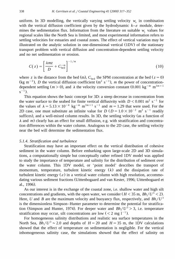
Results of 23 model sensitivity simulations in terms of the percentage change of theŽ .GoF with respect to a run with the above initial parameter settings run 0 are shown
graphically in Fig. 9.The largest relative difference results from a doubling of the input due to coastal
Ž .erosion at Holderness case 10 . The largest model improvement follows for doublingŽ .t case 4 , leading to a value t s1.5 Pa. This parameter value is rather high andc,ero c,ero
Fig. 9. Change of the GoF criterion in percentage for 23 sensitivity simulations with the 2D SPM model,Ž .relative to a reference simulation index 0 . Simulation period 1st March–1st October 1994.
( )H. Gerritsen et al.rCoastal Engineering 41 2000 317–352 341
suggests that erosion occurs only at high wind speed, andror in areas with much waveŽ .activity. Increasing l settling velocity by more than a factor of two gives rise to only a
Ž .small effect case 20 . Cases 9, 11 and 13, representing the effect of halving the assumedinput due to coastal erosion at Holderness, Suffolk and Norfolk, indicate that the inputs
Ž .should be less than those given in Odd and Murphy 1992 and perhaps more in lineŽ . Ž .with McCave 1987 and McManus and Prandle 1997 . There is no good explanation
yet why these results predict an increase of the dumping at Zeebrugge and OostendeŽ .case 16; doubling of the reference value . The results of case 23 confirm the modelassumption that erosion is not uniformly distributed over the year, and is correlated towind stress.
A further aspect is the present assumption of constant and spatial uniform parameters,which, e.g. for sedimentation and erosion parameters, will be too simple. More detailedexperimental information is required on the ranges of the various processes andparameters, including data on surficial bed sediments available for erosion. Improvedparameter formulations should be derived from such information.
The results highlight the complexities of suspended matter modelling. Fig. 9 showsŽ .six single parameter variations cases 4, 9, 13, 16, 21 and 23 that lead to a reduction of
Ž .more than 4% in the GoF criterion. Only one of these exceeds a 10% reduction case 4 .The present model variations are clearly insufficient for optimising the model in termsof adjusting the parameters to give a minimum value for the GoF criterion. Combinedvariations will need to be assessed, e.g. as outlined by the section on adjoint modellingŽ .see ten Brummelhuis et al., 2000; Vos et al., 2000 .
5.2.3. SensitiÕity analysis in 3DThe 3D sensitivity analysis focussed on the one concept that is essentially different
from 2D, namely the settling velocity w . Section 5.1.3 presented some concentration-s
dependent 2D formulations applied in estuaries. For 3D and regional scales, a depen-dence on concentration is unclear from the outset. The conceptual relation w slC m
sw ym 3mq1 y1 xwas retained, with l having dimension kg m day . Five simulations were
made, varying w , and results were compared with the 2D results, all for the periods
April–July 1994. The remaining basic model parameters are unchanged from the 2Dcase, apart from the bed stress assumption t s0, which however is expected to havewave
limited influence for the period of simulation. Table 6 defines the five 3D casesconsidered.
The first three simulations differ in the definition of w . We assume a seasonals
dependence of all coastal erosion inputs in simulations 4 and 5: the annual average atApril, half this value in July and an overall reduction to 72% for these 4 months. This isbecause of the large influence of coastal erosion in 2D and the conclusions relating to
Ž .the uncertainties in coastal inputs from the adjoint analysis in Vos et al. 2000 , and isbased on the seasonal distribution applied in simulation 23 of the previous subsection. In
Ž . Ž .these simulations, parameter settings ls5, ms0 and ls0.5, ms1 were as-sumed, respectively. Fig. 10 presents the results, using remote sensing data and surfacelayer model results in the GoF.
Ž .These results show that: 1 the reference simulation with a constant settling velocityy1 Žof 5 m day compares very well with the 2D model result a difference of 8% is
( )H. Gerritsen et al.rCoastal Engineering 41 2000 317–352342
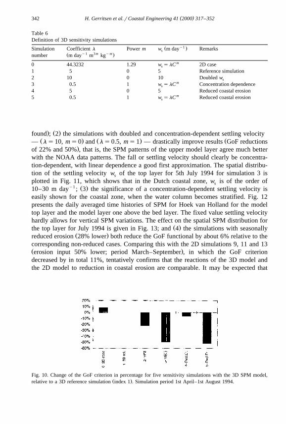
Table 6Definition of 3D sensitivity simulations
y1Ž .Simulation Coefficient l Power m w m day Remarkssy1 3m ymŽ .number m day m kg
m0 44.3232 1.29 w s lC 2D cases
1 5 0 5 Reference simulation2 10 0 10 Doubled ws
m3 0.5 1 w s lC Concentration dependences
4 5 0 5 Reduced coastal erosionm5 0.5 1 w s lC Reduced coastal erosions
. Ž .found ; 2 the simulations with doubled and concentration-dependent settling velocityŽ . Ž . Ž— ls10, ms0 and ls0.5, ms1 — drastically improve results GoF reductions
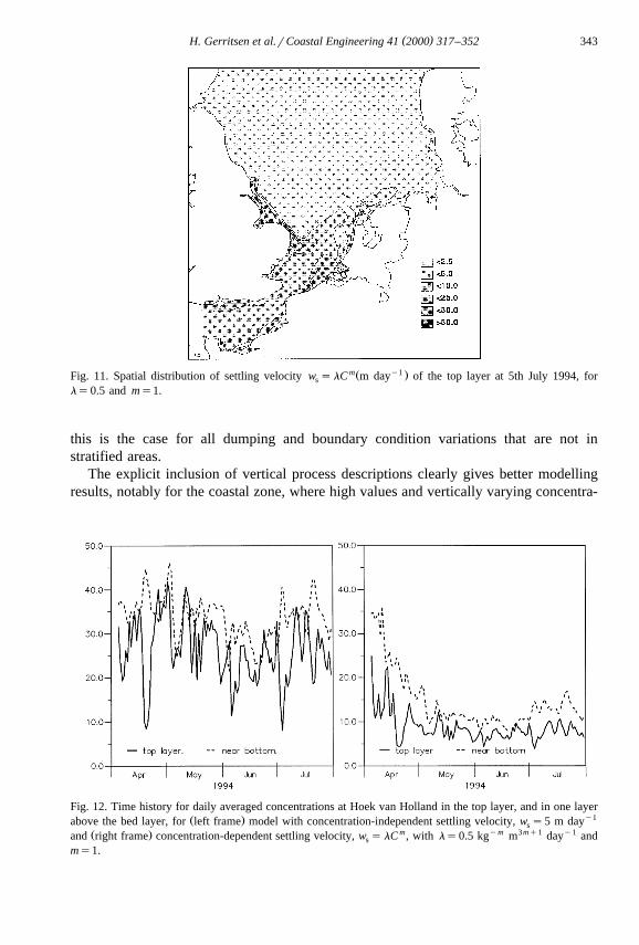
.of 22% and 50% , that is, the SPM patterns of the upper model layer agree much betterwith the NOAA data patterns. The fall or settling velocity should clearly be concentra-tion-dependent, with linear dependence a good first approximation. The spatial distribu-tion of the settling velocity w of the top layer for 5th July 1994 for simulation 3 iss
plotted in Fig. 11, which shows that in the Dutch coastal zone, w is of the order ofsy1 Ž .10–30 m day ; 3 the significance of a concentration-dependent settling velocity is
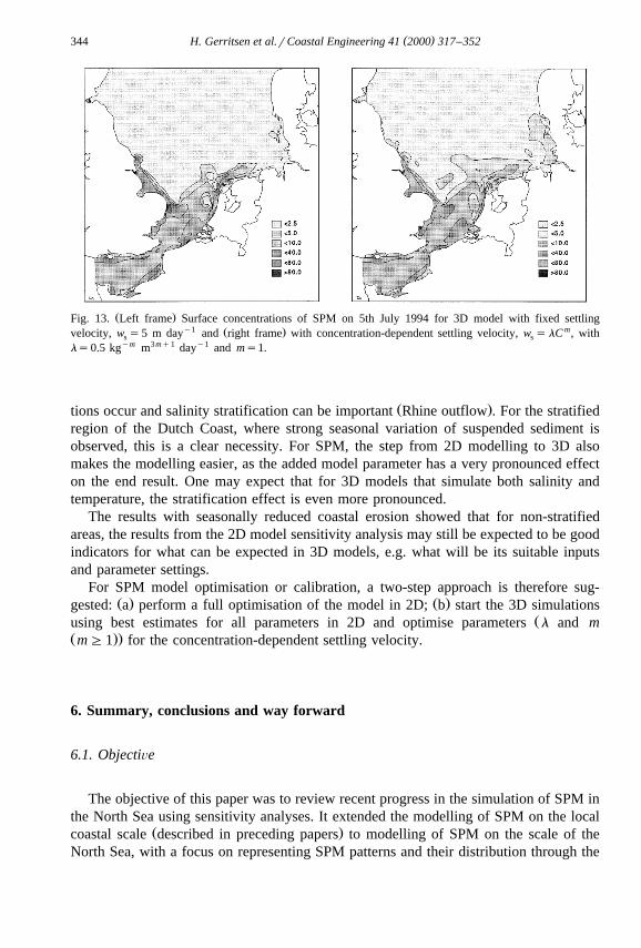
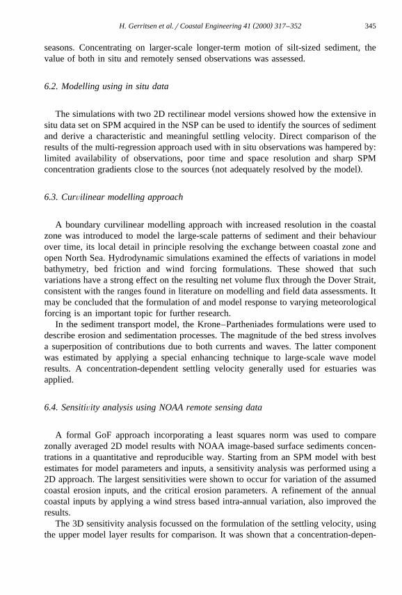
easily shown for the coastal zone, when the water column becomes stratified. Fig. 12presents the daily averaged time histories of SPM for Hoek van Holland for the modeltop layer and the model layer one above the bed layer. The fixed value settling velocityhardly allows for vertical SPM variations. The effect on the spatial SPM distribution for
Ž .the top layer for July 1994 is given in Fig. 13; and 4 the simulations with seasonallyŽ .reduced erosion 28% lower both reduce the GoF functional by about 6% relative to the
corresponding non-reduced cases. Comparing this with the 2D simulations 9, 11 and 13Ž .erosion input 50% lower; period March–September , in which the GoF criteriondecreased by in total 11%, tentatively confirms that the reactions of the 3D model andthe 2D model to reduction in coastal erosion are comparable. It may be expected that
Fig. 10. Change of the GoF criterion in percentage for five sensitivity simulations with the 3D SPM model,Ž .relative to a 3D reference simulation index 1 . Simulation period 1st April–1st August 1994.
( )H. Gerritsen et al.rCoastal Engineering 41 2000 317–352 343
mŽ y1 .Fig. 11. Spatial distribution of settling velocity w s lC m day of the top layer at 5th July 1994, fors
ls0.5 and ms1.
this is the case for all dumping and boundary condition variations that are not instratified areas.
The explicit inclusion of vertical process descriptions clearly gives better modellingresults, notably for the coastal zone, where high values and vertically varying concentra-
Fig. 12. Time history for daily averaged concentrations at Hoek van Holland in the top layer, and in one layerŽ . y1above the bed layer, for left frame model with concentration-independent settling velocity, w s5 m days
Ž . m ym 3mq1 y1and right frame concentration-dependent settling velocity, w s lC , with ls0.5 kg m day ands
ms1.
( )H. Gerritsen et al.rCoastal Engineering 41 2000 317–352344
Ž .Fig. 13. Left frame Surface concentrations of SPM on 5th July 1994 for 3D model with fixed settlingy1 Ž . mvelocity, w s5 m day and right frame with concentration-dependent settling velocity, w s lC , withs s
ls0.5 kgym m3mq1 dayy1 and ms1.
Ž .tions occur and salinity stratification can be important Rhine outflow . For the stratifiedregion of the Dutch Coast, where strong seasonal variation of suspended sediment isobserved, this is a clear necessity. For SPM, the step from 2D modelling to 3D alsomakes the modelling easier, as the added model parameter has a very pronounced effecton the end result. One may expect that for 3D models that simulate both salinity andtemperature, the stratification effect is even more pronounced.
The results with seasonally reduced coastal erosion showed that for non-stratifiedareas, the results from the 2D model sensitivity analysis may still be expected to be goodindicators for what can be expected in 3D models, e.g. what will be its suitable inputsand parameter settings.
For SPM model optimisation or calibration, a two-step approach is therefore sug-Ž . Ž .gested: a perform a full optimisation of the model in 2D; b start the 3D simulations
Žusing best estimates for all parameters in 2D and optimise parameters l and mŽ ..mG1 for the concentration-dependent settling velocity.
6. Summary, conclusions and way forward
6.1. ObjectiÕe
The objective of this paper was to review recent progress in the simulation of SPM inthe North Sea using sensitivity analyses. It extended the modelling of SPM on the local
Ž .coastal scale described in preceding papers to modelling of SPM on the scale of theNorth Sea, with a focus on representing SPM patterns and their distribution through the
( )H. Gerritsen et al.rCoastal Engineering 41 2000 317–352 345
seasons. Concentrating on larger-scale longer-term motion of silt-sized sediment, thevalue of both in situ and remotely sensed observations was assessed.
6.2. Modelling using in situ data
The simulations with two 2D rectilinear model versions showed how the extensive insitu data set on SPM acquired in the NSP can be used to identify the sources of sedimentand derive a characteristic and meaningful settling velocity. Direct comparison of theresults of the multi-regression approach used with in situ observations was hampered by:limited availability of observations, poor time and space resolution and sharp SPM
Ž .concentration gradients close to the sources not adequately resolved by the model .
6.3. CurÕilinear modelling approach
A boundary curvilinear modelling approach with increased resolution in the coastalzone was introduced to model the large-scale patterns of sediment and their behaviourover time, its local detail in principle resolving the exchange between coastal zone andopen North Sea. Hydrodynamic simulations examined the effects of variations in modelbathymetry, bed friction and wind forcing formulations. These showed that suchvariations have a strong effect on the resulting net volume flux through the Dover Strait,consistent with the ranges found in literature on modelling and field data assessments. Itmay be concluded that the formulation of and model response to varying meteorologicalforcing is an important topic for further research.
In the sediment transport model, the Krone–Partheniades formulations were used todescribe erosion and sedimentation processes. The magnitude of the bed stress involvesa superposition of contributions due to both currents and waves. The latter componentwas estimated by applying a special enhancing technique to large-scale wave modelresults. A concentration-dependent settling velocity generally used for estuaries wasapplied.
6.4. SensitiÕity analysis using NOAA remote sensing data
A formal GoF approach incorporating a least squares norm was used to comparezonally averaged 2D model results with NOAA image-based surface sediments concen-trations in a quantitative and reproducible way. Starting from an SPM model with bestestimates for model parameters and inputs, a sensitivity analysis was performed using a2D approach. The largest sensitivities were shown to occur for variation of the assumedcoastal erosion inputs, and the critical erosion parameters. A refinement of the annualcoastal inputs by applying a wind stress based intra-annual variation, also improved theresults.
The 3D sensitivity analysis focussed on the formulation of the settling velocity, usingthe upper model layer results for comparison. It was shown that a concentration-depen-
( )H. Gerritsen et al.rCoastal Engineering 41 2000 317–352346
Ž .dent settling velocity linear gives markedly better results than a fixed value, notably inthe coastal zone where salinity stratification may occur. Furthermore, the sensitivityanalysis to inputs and horizontal transport performed with the 2D modelling approachtends to remain valid for 3D model applications. It is concluded that for operationalmodelling and validation, 2D modelling would be a logical first step to a 3D modelset-up.
6.5. Conclusions
The above structured analysis and quantification of the effects of uncertainties ofinputs and sedimentationrerosion parameters using remote sensing-based concentrationdata has been shown to be feasible and useful. This analysis provides a much better
Ž .understanding of the uncertainties in sediment distribution and budgets on North Seascale and in the strengths and weaknesses of our modelling capabilities.
We can anticipate that process studies are likely to contribute to improvederosionrdeposition algorithms, and model developments will provide enhanced dynami-cal descriptions. However, accurate overall simulation will remain dependent on someŽ .inverse process to reduce the uncertainty in the observational data on sediment sources.
6.6. Specific modelling uncertainties
Ž .The fundamental uncertainties in modelling SPM fluxes arise from: i the dominantŽrole of sediment sources, information on which is often incomplete or inaccurate extent
. Ž . Ž .of source material and associated particle type spectra ; ii relatively simple bulkŽ .erosion and deposition formulae especially regarding the influence of flocculation ,
Ž .though in line with the observational information available for their validation; iiiŽ .insufficient information on bed surface sediments including seasonal variation avail-
able for resuspension.There are further inaccuracies associated with descriptions of tidal,surge and wave dynamics but these are generally relatively well-prescribed. However,the sensitivity of calculated net long-term advective volume fluxes to model character-istics and set-up remains significant. A key item here is the time-integrated response ofthe horizontal motion to fluctuating meteorological forcing with the general air–seamomentum transfer formulations.
6.7. Specific monitoring uncertainties
Ž .Available observations suffer from similar fundamental shortcomings, namely: icalibration from sensor units to concentration — including sensitivity to particle sizespectra in optical and acoustic instruments and to atmospheric corrections and sun angle
Ž . Ž .effects in remote sensing; ii unresolved particle-size spectra; iii limited spatial andtemporal coverage: remote sensing data provide high resolution spatially but for thesurface and at low resolution in time, whereas in situ instruments provide high temporal
( )H. Gerritsen et al.rCoastal Engineering 41 2000 317–352 347
resolution for the whole water column but only for single-points.Thus, the fundamentaldifficulties in simulating SPM transports arise from limited descriptions of key inputs
Ž .and processes coastal erosion, rates of sediment erosion and deposition and limitedaccuracy in the resolution and parameter range of observations. Under these circum-stances, simple simulation models are appropriate. However, despite the general incom-patibility between resolution provided by observations and that which is now possible inmodels, the clear association of major SPM events in specific locations with particular
Ždynamical conditions e.g. wind–wave stirring, major residual flows, stratification,.extreme river discharges, etc. can provide clear support for model refinement.
6.8. Key model refinements
The analysis and intercomparisons described here illustrate the usefulness and oftenŽ .the need, even within the strategy of minimal modelling, for: i fine grid resolution in
Ž . Ž . Ž .key coastal areas; ii fully 3D dynamics reducing empiricism in deposition formulae ;Ž . Ž .iii inclusion of wind–wave effects on bed stress shallow areas .
6.9. Future challenges
The rapid recent developments in modelling of the dynamics of tides, surges andwaves have been noted. Generally, the performance of these models is now limited bythe provision of related bathymetry, air–sea momentum transfer and, especially, seabedand coastal sediment data. Thus, integrated modelling-monitoring strategies exploitinginverse modelling and assimilationrGoF techniques are likely to be necessary for theforeseeable future. Progress in atmospheric corrections and in improved calibration ofremote sensing data is likely both from advances in basic physics, enhanced spectralresolution of sensors and via synergistic usage of in situ sensors. However, the watersurface limitation of remote sensing will remain and thus further development of depthprofiling and side-sweeping acoustic instrumentation is similarly important. Studies ofbasic processes in near-full scale of fluxes etc. will continuously enhance our under-standing of the relationships between tide- and wave-induced stresses and associatedsediment erosion.
Acknowledgements
The present work was funded by the EU MAST III project PROMISE under contractnumber MAS3-CT950025 and co-funded by WLrDelft Hydraulics’ basic researchprogramme. The authors gratefully acknowledge the permission of the Royal Nether-lands Meteorological Institute for use of the NOAArAVHRR data, and that of theNorwegian Meteorological Institute to use their historic wind and pressure data. Theauthors thank the WASA group and Marek Stawarz of GKSS for making availableresults of the WASA wave modelling study and Jean-Claude Salomon of IFREMER for
( )H. Gerritsen et al.rCoastal Engineering 41 2000 317–352348
bathymetry data. Last but not least, we thank David Prandle at POL and Gerbrant vanVledder, formerly at Delft Hydraulics, for the constructive discussions on the presentwork.
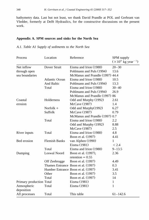
Appendix A. SPM sources and sinks for the North Sea
A.1. Table A1 Supply of sediments to the North Sea
Process Location Reference SPM supply9 y1Ž .=10 kg year
Ž .Net inflow Dover Strait Eisma and Irion 1988 20–30Ž .through open Pohlmann and Puls 1994 13.6
Ž .sea boundaries McManus and Prandle 1997 44.4Ž .Atlantic Ocean Eisma and Irion 1988 10.5
Ž .And Baltic Pohlmann and Puls 1994 13.3Ž .Total Eisma and Irion 1988 30–40
Ž .Pohlmann and Puls 1994 26.9Ž .McManus and Prandle 1997 86
Ž .Coastal Holderness Odd and Murphy 1992 2.61Ž .erosion McCave 1987 1.4
Ž .Norfolkq Odd and Murphy 1992 6.27Ž .Suffolk McCave 1987 0.79
Ž .McManus and Prandle 1997 0.7Ž .Total Eisma and Irion 1988 2.2Ž .Odd and Murphy 1992 8.88
Ž .McCave 1987 2.5Ž .River inputs Total Eisma and Irion 1988 4.8
Ž .Boon et al. 1997 4.41Ž .Bed erosion Flemish Banks van Alphen 1990 1
Ž .Eisma 1981 -2.4Ž .Total Eisma and Irion 1988 9–13.5
Ž .Dumping Loswal Noord Boon et al. 1997 , 2.36retentions0.55
Ž .Off Zeebrugge Boon et al. 1997 4.49Ž .Thames Entrance Boon et al. 1997 0.3Ž .Humber Entrance Boon et al. 1997 3.41Ž .Other Boon et al. 1997 3.5Ž .Total Boon et al. 1997 14
Ž .Primary production Total Eisma 1981 1Ž .Atmospheric Total Eisma 1981 1
depositionAll processes Total This table 61–142.6
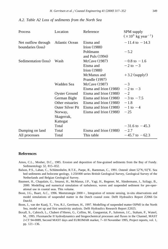
( )H. Gerritsen et al.rCoastal Engineering 41 2000 317–352 349
A.2. Table A2 Loss of sediments from the North Sea
Process Location Reference SPM supply9 y1Ž .=10 kg year
Net outflow through Atlantic Ocean Eisma and y11.4 to y14.3Ž . Ž .boundaries loss Irion 1988
Pohlmann y5.2Ž .and Puls 1994
Ž . Ž .Sedimentation loss Wash McCave 1987 y0.8 to y1.6Eisma and y2 to y3
Ž .Irion 1988Ž .McManus and q3.2 supply!
Ž .Prandle 1997Ž .Wadden Sea McCave 1987 y3
Ž .Eisma and Irion 1988 y2 to y3Ž .Oyster Ground Eisma and Irion 1988 y2Ž .German Bight Eisma and Irion 1988 y3 to y7.5Ž .Other estuaries Eisma and Irion 1988 y1.8Ž .Outer Silver Pit Eisma and Irion 1988 y1 to y4Ž .Norway, Eisma and Irion 1988 y25
Skagerrak,KattegatTotal y31.6 to y45.3
Ž .Dumping on land Total Eisma and Irion 1988 y2.7All processes Total This table y45.7 to y62.3
References
Amos, C.L., Mosher, D.C., 1985. Erosion and deposition of fine-grained sediments from the Bay of Fundy.Sedimentology 32, 815–832.
Balson, P.S., Laban, C., Schuttenhelm, R.T.E., Paepe, R., Baeteman, C., 1991. Ostend: sheet 528Nr028E. Sea¨bed sediments and holocene geology, 1:250000 series British Geological Survey, Geological Survey of theNetherlands and Belgian Geological Survey.
Baumert, H., Chapalain, G., Smaoui, H., McManus, J.P., Yagi, H., Regener, M., Sundermann, J., Szilagy, B.,¨2000. Modelling and numerical simulation of turbulence, waves and suspended sediment for pre-oper-ational use in coastal seas. This volume.
Boon, J.G., Baart, A.C., 1996. Meetstrategie 2000q, Integration of remote sensing, in-situ observations andŽmodel simulations of suspended matter in the Dutch coastal zone. Delft Hydraulics Report Z2066 in
.Dutch .Ž .Boon, J., van der Kaaij, T., Vos, R.J., Gerritsen, H., 1997. Modelling of suspended matter SPM in the North
Sea, model set up and first sensitivity analysis. Delft Hydraulics Research Report Z2025.Boxall, S., Cabioch, L., Chabert d’Hieres, G., Collins, M., Guegueniat, P., Salomon, J.C., Staham, P., Waterl,
M., 1995. Fluxmanche II hydrodynamics and biogeochemical processes and fluxes in the Channel, MAST2-CT 94-0089, Second MAST days and EUROMAR market, 7–10 November 1995, Project reports, vol. 1,pp. 121–136.
( )H. Gerritsen et al.rCoastal Engineering 41 2000 317–352350
Ž . Ž .British Geological Survey BGS . Sea bed sediments around the United Kingdom north and south sheets .Scale 1:1000000.
Ž .Burt, T.N., 1986. Field settling velocities of estuary muds. In: Mehta, A.J. Ed. , Estuarine Cohesive SedimentDynamics. Lecture Notes on Coastal and Estuarine Studies vol. 14 Springer, Berlin, pp. 126–150.
Chapalain, G., Thais, L., 2000. Tide, turbulence and suspended sediment modelling in the eastern EnglishChannel. This volume.
de Kok, J.M., 1992. A three-dimensional finite difference model for computation of near- and far-fieldŽ .transport of suspended matter near a river mouth. Continental Shelf Research 12 5r6 , 625–642.
Delft3D, 1997. Delft 3D-modelling system, User and Reference Manuals. Delft Hydraulics.Eisma, D., 1981. The mass balance of suspended matter and associated pollutants in the North Sea. Rapports
et Proces-Verbaux des Reunions — Conseil International pour l’Exploration de la Mer 181, 7–14.Eisma, D., Irion, G., 1988. Suspended matter and sediment transport. In: Salomons, W., Bayne, B.L.,
Ž .Duursma, E.K., Forstner, U. Eds. , Pollution of the North Sea: An Assessment. Springer, Berlin, pp.¨20–35.
Figge, K., 1981. Karte der Sedimentverteilung in der Deutschen Bucht, Nordsee. Deutsches HydrographischesŽ .Institut, Karte Nr. 2900 mit beiheft , Hamburg. Area: German Bight, western boundary 6 degrees E,
northern boundary 55805X N. Scale 1:250000. Mercator Projection. Content: grain size distribution of theuppermost 10 cm.
Geological Survey of the Netherlands, 1986. Raw materials at or near the surface.Gerritsen, H., Boon, J.G., van der Kaaij, Th., Vos, R.J., 2000. Integrated modelling of suspended particulate
matter in the North Sea. Estuarine, Coastal and Shelf Science, submitted for publication.Jarke, J., 1956. Der Boden der sudlichen Nordsee. Eine neue Bodenkarte der sudlichen Nordsee. Deutsche
Hydrographische Zeitschrift 9, 1–9.Johannessen, O.M., Sandven, S., Jenkins, A.D., Durand, D., Petterssen, L.H., Espedal, H., Evensen, G.,
Hamre, T., 2000. Satellite earth observation in operational oceanography. This volume.Jones, J.E., 1999. POL-2G. Proudman Oceanographic Laboratory 2D General Purpose Model. Proudman
Oceanographic Laboratory Internal Document No. 131.Kappe, B.P., van Koningsbruggen, P., Voogt, L., 1989. Erosion of silt resulting from navigation, extended.
Ž .Report series Integrated Water Management Ketelmeer. Rijkswaterstaat RIZA, Lelystad, in Dutch .Krone R.B., 1962. Flume studies of the transport of sediment in estuarial shoaling processes, Final report,
University of California, Hydraulic Engineering Laboratory and Sanitary Engineering Research Labora-tory, Berkeley, CA, USA.
Lane, A., Riethmuller, R., Herbers, D., Rybaczok, P., Gunther, H., Baumert, H., 2000. Observational data sets¨ ¨for model development. This volume.
Lehmann, H.J, Radach, G., Backhaus, J.O., Pohlmann, T., 1995. Simulations of the North Sea circulation, itsvariability and its implementation as hydrodynamic forcing in ERSEM. Netherlands Journal of SeaResearch 33, 271–299.
Ž .McCave, I.N., 1987. Fine sediment sources and sinks around the East Anglian Coast UK . Journal of theŽ .Geological Society London 144, 149–152.
McManus, J.P., Prandle, D., 1997. Development of a model to reproduce observed suspended sedimentdistributions in the southern North Sea using Principal Component Analysis and Multiple Linear
Ž .Regression. Continental Shelf Research 17 7 , 761–778.Mehta, A.J., 1986. Characterisation of cohesive sediment properties and transport processes in estuaries.
Ž .Estuarine Cohesive Sediment Dynamics. In: Mehta, A.J. Ed. , Lecture Notes on Coastal and EstuarineStudies 14 Springer, Berlin, pp. 290–325.
Mehta, A.J., Parchure, T.M., Dixit, J.G., Ariathurai, R., 1982. Resuspension potential of deposited cohesiveŽ .sediment beds. In: Kennedy, V.S. Ed. , Estuarine Comparisons. Academic Press, New York, pp. 591–609.
Monbaliu, J., Padilla-Hernandez, R., Hargreaves, J.C., Carretero Albiach, J.C., Luo, W., Sclavo, M., Gunther,´ ¨H., 2000. The spectral wave model WAM adapted for applications with high spatial resolution. Thisvolume.
Monbaliu, J., Hargreaves, J.C., Carretero, J.C., Gerritsen, H., Flather, R., 1999. Wave modelling in thePROMISE project. Coastal Engineering 37, 379–407.
Natural Environment Research Council, 1992. North Sea Project data set. CD ROM, British OceanographicData Centre, Proudman Oceanographic Laboratory, UK.
( )H. Gerritsen et al.rCoastal Engineering 41 2000 317–352 351
Nicholson, J., O’Connor, B.A., 1986. Cohesive sediment transport model. Journal of Hydraulic EngineeringŽ .112 7 , 621–640.
Odd N.V.M., Murphy, D.G., 1992. Particulate pollutants in the North Sea. Report SR 292, HydraulicsResearch, Wallingford.
Ozer, J., Padilla-Hernandez, R., Monbaliu, J., Alvarez Fanjul, E., Carretero Albiach, J.C., Osuna, P., Yu,´J.C.S., Wolf, J., 2000. A coupling module for tides, surges and waves. This volume.
Partheniades E., 1962. A study of erosion and deposition of cohesive soils in salt water, PhD dissertation,University of California, USA.
Ž .Pohlmann, T., Puls, W., 1994. Currents and transport in water. In: Sundermann, J. Ed. , Circulation and¨Contaminant Fluxes in the North Sea. Springer, Berlin, Section 3.2.
Prandle, D., 1978. Residual flows and elevations in the Southern North Sea. Proceedings of the Royal SocietyLondon, Series A 259, 189–228.
Prandle, D., 1984. A modelling study of the mixing of 137Cs in the seas of the European continental shelf.Philosophical Transactions of the Royal Society of London, Series A 310, 407–436.
Prandle, D., 1998. Tidal characteristics of suspended sediment concentrations. Journal of Hydraulic Engineer-Ž .ing 123 4 , 341–350.
Prandle, D., Ballard, G., Flatt, D., Harrison, A.J., Jones, S.E., Knight, P.J., Loch, S., McManus, J., 1996.Combining modelling and monitoring to determine fluxes of water, dissolved and particulate metalsthrough Dover Strait. Continental Shelf Research 16, 237–257.
Prandle, D., Hydes, D.J., Jarvis, J., McManus, J., 1997. The seasonal cycles of temperature, salinity, nutrientsand suspended sediment in the Southern North Sea in 1988 and 1989. Estuarine, Coastal and Shelf Science45, 669–680.
Prandle, D., Hargreaves, J.C., McManus, J.P., Campbell, A.R., Duwe, K., Lane, A., Mahnke, P., Shimwell, S.,Wolf, J., 2000. Tide, wave and suspended sediment modelling on an open coast — Holderness. Thisvolume.
Puls, W., Kuhl, H., Heymann, K., 1988. Settling velocity of mud flocs: results of field measurements in the¨Ž .Elbe and Weser estuary. In: Dronkers, J., van Leussen, W. Eds. , Physical Processes in Estuaries.
Springer, Berlin, pp. 404–426.Ž .Salomon, J.C., Breton, M., 1993. An atlas of long-term currents in the Channel. Oceanologica Acta 16 5–6 ,
438–439.Salomon, J.C., Breton, M., Guegueniat, P., 1993. Computed residual flow through the Dover Strait.
Ž .Oceanologica Acta 16 5–6 , 449–455.Salomon, J.C., Breton, M., Guegueniat, P., 1995. A 2D long term advection–dispersion model for the Channel
and southern North Sea: Part B. Transit time and transfer function from Cap de La Hague. Journal ofMarine Systems 6, 515–527.
Schneggenburger, C., Gunther, H., Rosenthal, W., 2000. Spectral wave modelling with non-linear dissipation:¨validation and application in a coastal tidal environment. This volume.
Simpson, J.H., Hunter, J.R., 1974. Fronts in the Irish Sea. Nature 250, 404–406.Ž .Sundermann, J. Ed. , Circulation and Contaminant Fluxes in the North Sea, Springer, Berlin.¨
ten Brummelhuis P.G.J., Gerritsen, H., van der Kaaij, T., 1997. Sensitivity analysis and calibration of thehydrodynamic PROMISE model using adjoint modelling techniques, Delft Hydraulics Research ReportZ2025.
ten Brummelhuis, P.G.J., Vos, R.J., Gerritsen, H., 2000. Skill assessment of transport models using the adjointtechnique. Estuarine, Coastal and Shelf Science, submitted for publication.
Thorn, M.F.C., 1981. Physical processes of siltation in tidal channels. Proceedings of Hydraulic Modellingapplied to Maritime Engineering Problems. ICE, London, 47–55.
Uittenbogaard, R.E., van Kester, J.A.Th.M., 1996. Modelling seasonal temperature stratification with TRI-WAQ. Delft Hydraulics Report Z978.
Uittenbogaard R.E., van Kester, J.A.Th.M., Stelling, G.S., 1992. Implementation of three turbulence models inTRISULA for rectangular horizontal grids. Delft Hydraulics Report Z162.
Uittenbogaard R.E., Winterwerp, J.C., van Kester, J.A.Th.M., Leepel, H., 1996. 3D Cohesive SedimentTransport parts I and II. Delft Hydraulics Report Z1022.
van Alphen, J.S.L.J., 1987. Silt occurrence on the Dutch and Belgian continental shelf sections. Rijkswater-Ž .staat, North Sea Directorate, Internal Document Nr. NZ-N-87.09b in Dutch .
( )H. Gerritsen et al.rCoastal Engineering 41 2000 317–352352
van Alphen, J.S.L.J., 1990. A mud balance for the Belgian–Dutch coastal waters between 1969 and 1986.Netherlands Journal of Sea Research 25, 19–30.
van Leussen, W., 1994. Estuarine macroflocs and their role in fine-grained sediment transport. PhD Thesis,University of Utrecht.
van Raaphorst, W., Philippart, C.J.M., Smits, J.P.C., Dijkstra, F.J., Malschaert, J.F.P., 1998. Distribution ofsuspended particulate matter in the North Sea as inferred from NOAArAVHRR reflectance images and insitu observations. Journal of Sea Research 39, 197–215.
van Rijn, L.C., 1993. Principles of Sediment Transport in Rivers, Estuaries and Coastal Seas. AquaPublications, Amsterdam.
van Vledder, G., 1997. Transformation of wave conditions from the WASA grid to the PROMISE grid andtheir parameterisation in the bed stress. Delft Hydraulics Research Report Z2025.
Vos R.J., Schuttelaar M., 1995. RESTWAQ, Data assessment, data-model integration and application to theSouthern North Sea, BCRS report 95-19, Delft, The Netherlands.
Vos, R.J., Schuttelaar, M., 1997. An integrated data-model system to support monitoring and assessment ofŽ .marine systems. In: Stel, J.H. Ed. , Proceedings of the First International Conference on EuroGOOS,
Elsevier Oceanography Series 62, The Hague, Netherlands, pp. 507–515.Vos, R.J., ten Brummelhuis, P.G.J., Gerritsen, H., 2000. Integrated data-modelling approach for suspended
sediment on a regional scale. This volume.WASA Group, 1995. The WASA project: changing storm and wave climate in the Northeast Atlantic and
adjacent seas. Proceedings of the 4th International Workshop on Wave Hindcasting and Forecasting, Banff,Canada.
Winterwerp, J.C, 1989. Flow-induced erosion of cohesive beds; a literature study. Rijkswaterstaat — DelftHydraulics Report No. 25.
Related Documents