JSS Journal of Statistical Software August 2013, Volume 54, Issue 11. http://www.jstatsoft.org/ survPresmooth: An R Package for Presmoothed Estimation in Survival Analysis Ignacio L´ opez-de-Ullibarri Universidade da Coru˜ na M. Amalia J´ acome Universidade da Coru˜ na Abstract The survPresmooth package for R implements nonparametric presmoothed estimators of the main functions studied in survival analysis (survival, density, hazard and cumulative hazard functions). Presmoothed versions of the classical nonparametric estimators have been shown to increase efficiency if the presmoothing bandwidth is suitably chosen. The survPresmooth package provides plug-in and bootstrap bandwidth selectors, also allowing the possibility of using fixed bandwidths. Keywords : nonparametric estimation, presmoothing, R. 1. Introduction Survival analysis is oriented to the study of the random time (lifetime, failure time) T from an initial point to the occurrence of some event of interest. An important goal is to estimate the functions that characterize the distribution of T (in the following, assumed to be absolutely continuous): (a) the distribution function, F (t)= P (T ≤ t) or, equivalently, the survival function, S (t)=1 - F (t), (b) the density function, f (t)= F 0 (t), c) the hazard function, λ(t) = lim Δt→0 + P (t ≤ T<t +Δt|T ≥ t)/Δt = f (t)/S (t) and d) the cumulative hazard function, Λ(t)= R t 0 λ(v)dv, for t> 0. The handling of incomplete observations is one of the major problems one has to face in the analysis of lifetimes. Typically, the true lifetimes are incompletely observed due to censoring. In the right censoring (RC) model, the lifetime T can be observed only if its value is smaller than that of an independent censoring variable C . Thus, based on a random sample (T i ,C i ), i =1,...,n, the actual information for the ith observation is conveyed by the pair (Z i ,δ i ), where Z i = min(T i ,C i ) is the observed time and δ i = 1 {T i <C i } indicates whether the observation is censored (δ i = 0) or not (δ i = 1). Posed in statistical terms, the problem is how to estimate the different functionals of the lifetime T using the observed (Z, δ). Classical nonparametric estimators in the presence of

Welcome message from author
This document is posted to help you gain knowledge. Please leave a comment to let me know what you think about it! Share it to your friends and learn new things together.
Transcript
JSS Journal of Statistical SoftwareAugust 2013, Volume 54, Issue 11. http://www.jstatsoft.org/
survPresmooth: An R Package for Presmoothed
Estimation in Survival Analysis
Ignacio Lopez-de-UllibarriUniversidade da Coruna
M. Amalia JacomeUniversidade da Coruna
Abstract
The survPresmooth package for R implements nonparametric presmoothed estimatorsof the main functions studied in survival analysis (survival, density, hazard and cumulativehazard functions). Presmoothed versions of the classical nonparametric estimators havebeen shown to increase efficiency if the presmoothing bandwidth is suitably chosen. ThesurvPresmooth package provides plug-in and bootstrap bandwidth selectors, also allowingthe possibility of using fixed bandwidths.
Keywords: nonparametric estimation, presmoothing, R.
1. Introduction
Survival analysis is oriented to the study of the random time (lifetime, failure time) T from aninitial point to the occurrence of some event of interest. An important goal is to estimate thefunctions that characterize the distribution of T (in the following, assumed to be absolutelycontinuous): (a) the distribution function, F (t) = P (T ≤ t) or, equivalently, the survivalfunction, S(t) = 1 − F (t), (b) the density function, f(t) = F ′(t), c) the hazard function,λ(t) = lim∆t→0+ P (t ≤ T < t + ∆t|T ≥ t)/∆t = f(t)/S(t) and d) the cumulative hazardfunction, Λ(t) =
∫ t0 λ(v)dv, for t > 0. The handling of incomplete observations is one of the
major problems one has to face in the analysis of lifetimes. Typically, the true lifetimes areincompletely observed due to censoring. In the right censoring (RC) model, the lifetime Tcan be observed only if its value is smaller than that of an independent censoring variableC. Thus, based on a random sample (Ti, Ci), i = 1, . . . , n, the actual information for the ithobservation is conveyed by the pair (Zi, δi), where Zi = min(Ti, Ci) is the observed time andδi = 1{Ti<Ci} indicates whether the observation is censored (δi = 0) or not (δi = 1).
Posed in statistical terms, the problem is how to estimate the different functionals of thelifetime T using the observed (Z, δ). Classical nonparametric estimators in the presence of
2 survPresmooth: Presmoothed Estimation in Survival Analysis in R
right censoring are well established in the literature. The Kaplan-Meier (KM) estimator ofthe survival function (Kaplan and Meier 1958), the kernel estimator of the density with KMweights (Foldes, Rejto, and Winter 1981), the kernel estimator of the hazard function byTanner and Wong (1983) and the Nelson-Aalen (NA) estimator of the cumulative hazardfunction (Nelson 1972; Aalen 1978) are a representative selection of this type of estimators.A general account of these estimators can be found in standard texts on survival analysis (seee.g., Klein and Moeschberger 2003).
To motivate the presmoothing procedures, note that the KM and NA estimators are stepfunctions with jumps located only at the uncensored observations. Therefore, when manydata are censored, the KM and NA estimators have only a few jumps with increasing sizesand the accuracy of the estimation might not be acceptable. Heavily censored data sets arebecoming more frequent, since developments lead to increasing lifetimes, and if the testingtime is not enlarged (and it usually can not be enlarged), an increase in lifetimes leads toincreasing censoring. In such a situation, more efficient competitors for the classical estimatorsare essential. The presmoothed estimators are a good alternative, since they are computed bygiving mass to all the data, including the censored observations. Central to the idea behindpresmoothing is the function p(t) = P (δ = 1|Z = t), i.e., the conditional probability that theobservation at time t is not censored. The function p depends on the observable variables(Z, δ), and for this reason, it can be easily estimated. Another important feature of p is thatfunctionals of the incomplete lifetimes T can be expressed in terms of p(t) and functions ofthe observed (Z, δ). For example, for the cumulative hazard rate we have
Λ(t) =
∫ t
0
p(u)dH(u)
1−H(u−),
where H denotes the distribution function of Z. The classical NA estimator of Λ is obtainedby replacing H with its empirical estimator Hn and the value of p(Zi) by the correspondingindicator of non-censoring δi, giving rise to a step function with jumps only at the uncensoreddata:
ΛNAn (t) =1
n
∑i:Zi≤t
δi1−Hn(Zi) + 1/n
. (1)
The straightforward idea on which the presmoothed estimators are based is to consider asmoother estimator of p(Zi) rather than δi. This has important implications:
(a) The new estimators are computed by giving mass to each observation regardless ofwhether it is censored or not. Thus, more information on the local behavior of thelifetime distribution is provided. The accuracy of the estimation is then increased,above all for heavily censored data.
(b) Using the smooth estimator of p, the available information can be extrapolated to betterdescribe the tail behavior.
Since δ is a dichotomic variable, p can also be written as a regression function p(t) = E(δ|Z =t). Thus, p can be estimated parametrically (e.g., using a logistic fit) or nonparametrically, forexample, using the Nadaraya-Watson (NW) kernel estimator (Nadaraya 1964; Watson 1964)
Journal of Statistical Software 3
with bandwidth b1:
pb1(t) =
n∑i=1
Kb1(t− Zi)δin∑i=1
Kb1(t− Zi), (2)
where K is a kernel function and Kb(t) = b−1K(t/b) denotes the rescaled kernel. TypicallyK is a symmetric density function compactly supported, without loss of generality, in theinterval [−1, 1].
Estimation of S and Λ with a logistic fit of p has been studied by Dikta (1998, 2000, 2001).It is shown in Dikta (1998) that, when the parametric model assumed for p is correct, thissemiparametric estimator of S is at least as efficient as the KM estimator in terms of theasymptotic variance. As a drawback, there is a clear risk of a miss-specification of the para-metric model for p.
The presmoothed approach is based on the NW estimator of p, and has been extensivelystudied in the literature in the estimation of S and Λ (Cao, Lopez-de-Ullibarri, Janssen, andVeraverbeke 2005), the density f (Cao and Jacome 2004; Jacome and Cao 2007; Jacome,Gijbels, and Cao 2008), the hazard rate λ (Cao and Lopez-de-Ullibarri 2007), and also thequantile function (Jacome and Cao 2008) (for an illustration of the use of nonparametricregression estimators other than the NW smoother, see Jacome et al. 2008). Nonparametrickernel regression, as the NW estimator, does not requires preliminary specification of a para-metric family. In contrast, a bandwidth b1 must be chosen for the computation of pb1(t). Notethat when the bandwidth is very small then pb1(Zi) ' δi, and the presmoothed estimatorsreduce to the classical ones.
The beneficial effect of presmoothing depends, as expected, on the choice of the presmooth-ing bandwidth b1. When the asymptotically optimal bandwidth is used, the presmoothedestimators have smaller asymptotic variance and, therefore, a better performance in termsof mean squared error (MSE). This improvement is of second order in the estimation of Sand Λ (Cao et al. 2005), but may be of first order for the density function (Cao and Jacome2004). The simulation studies confirm this gain in efficiency under moderate sample sizes.Moreover, they also show that the presmoothed estimators are better than the classical ones,not only for the optimal value of the bandwidth but for quite wide ranges of values of b1.A comparison of the semiparametric and presmoothed estimators of S has been carried outunder left truncation and right censored (LTRC) data by Jacome and Iglesias-Perez (2008),where the nice behavior of both estimators, with respect to the classical one, is shown ina simulation study. Specifically, the presmoothed estimator has a better performance thanthe classical estimator in the complete interval of computation, and than the semiparametricestimator for inner points, while the improvement vanishes in the boundary of the interval.In summary, this good performance suggests that presmoothing is a competitive method thatmay outperforms the classical estimators.
The survPresmooth package (Lopez-de-Ullibarri and Jacome 2013) provides an implementa-tion in R (R Core Team 2013) of the presmoothed estimators of the functions S, f , λ andΛ in the RC model, including methods for bandwidth selection and correction of possibleboundary effects.
Our main purpose on writing this paper was twofold: (a) to introduce the survPresmoothpackage to R users, providing at the same time a review of presmoothing techniques; and (b) to

4 survPresmooth: Presmoothed Estimation in Survival Analysis in R
show the performance of presmoothed estimators both in the analysis of a real dataset and insimulated scenarios. The presmoothed estimators implemented in the package are reviewedin Section 2. The two following sections deal with additional technical aspects of presmooth-ing, like bandwidth-parameter selection (Section 3) or boundary-effect correction (Section 4).In Section 5, after describing the package functions, the implemented presmoothed estima-tion procedures are applied to a real dataset and their performance is shown by means of asimulation study. Some concluding remarks are given in Section 6.
2. Presmoothed estimators
Survival and distribution functions
The presmoothed estimator of the survival function S (Jacome and Cao 2007) is
SPb1(t) =∏i:Zi≤t
(1− pb1(Zi)
n(1−Hn(Zi) + 1/n)
).
It can be derived from the KM estimator,
SKMn (t) =∏i:Zi≤t
(1− δi
n(1−Hn(Zi) + 1/n)
),
just by replacing δi with the value at point Zi of the NW estimate of p in Equation 2. Anobvious presmoothed estimator of the distribution function F is FPb1 = 1− SPb1 .
The estimator SPb1 is a decreasing step function, with jumps at the observed (censored or
uncensored) times. In this aspect it differs from SKMn , whose jumps are restricted to theuncensored times. Two further properties relating the presmoothed estimator with its classicalcounterpart should be mentioned. Firstly, when b1 ↓ 0, then SPb1 coincides in the limit with
SKMn . Secondly, when there is no censoring, SPb1 reduces to the empirical estimator of S.
Density function
If F is estimated by a step function F , the density f = F ′ can be estimated by smoothingthe increments of F . This is the idea behind the most popular nonparametric estimator of f ,Parzen-Rosenblatt’s (PR) kernel density estimator (Parzen 1962; Rosenblatt 1956):
fb2(t) =
∫ ∞0
Kb2(t− u)dF (u) (3)
where b2 ≡ b2n ↓ 0 is the smoothing parameter and K a kernel function.
If, for example, F ≡ FKMn = 1 − SKMn , simple calculations show that the estimator inEquation 3 takes the form
fKMb2 (t) =
n∑i=1
Kb2(t− Z(i))WKM(i) ,
where Z(i) denotes the ith ordered observation and the weights WKM(i) are defined as WKM
(i) =
FKMn (Z(i)) − FKMn (Z(i−1)). This is the density estimator proposed by Foldes et al. (1981).

Journal of Statistical Software 5
Note that without censoring, WKM(i) = 1/n and Zi = Ti for i = 1, . . . , n. Then, the well-known
kernel estimator for uncensored data, fb2(t) =∑n
i=1Kb2(t− Ti)/n, is recovered.
In a similar way, if FPb1 is used to estimate F , a presmoothed estimator of the density functionis obtained:
fPb1,b2(t) =
∫ ∞0
Kb2(t− u)dFPb1 (u) =n∑i=1
Kb2(t− Z(i))WP(i),b1
, (4)
where WP(i),b1
= FPb1 (Z(i)) − FPb1 (Z(i−1)). This estimator depends on two parameters: the
presmoothing bandwidth b1, needed to compute pb1 , and a smoothing bandwidth b2. Key
properties of fPb1,b2 , such as its asymptotic normality and an almost sure asymptotic repre-sentation, are proved in Cao and Jacome (2004), Jacome and Cao (2007) and Jacome et al.(2008).
Hazard function and cumulative hazard function
There is a rich literature on nonparametric hazard function estimation. Here we restrict our-selves to the estimator proposed by Tanner and Wong (1983) for right-censored data. Notingthat λ = Λ′ the Tanner-Wong estimator (TW), very similar to the independent proposals byRamlau-Hansen (1983) and Yandell (1983), is obtained by smoothing the increments of theNA estimator in Equation 1:
λb2(t) =
∫ ∞0
Kb2(t− u)dΛNAn (u) =1
n
n∑i=1
Kb2(t− Zi)δi1−Hn(Zi) + 1/n
.
As was pointed out in Section 1, the presmoothed NA estimator of the cumulative hazardfunction results from substituting δi with pb1(Zi), and is defined by:
ΛPb1(t) =1
n
∑i:Zi≤t
pb1(Zi)
1−Hn(Zi) + 1/n.
An asymptotic representation and asymptotic distributional properties of ΛPb1 can be foundin Cao et al. (2005). Some evidence of the beneficial effect of presmoothing is also providedin that reference.
Following the same ideas leading to Equation 4 in the density case, a presmoothed version ofthe Tanner-Wong estimator of λ (Cao and Lopez-de-Ullibarri 2007) can be obtained:
λPb1,b2(t) =
∫ ∞0
Kb2(t− u)dΛPb1(u) =1
n
n∑i=1
Kb2(t− Zi)pb1(Zi)
1−Hn(Zi) + 1/n. (5)
Like the presmoothed density estimator, λPb1,b2 also depends on two parameters, b1 and thesmoothing bandwidth b2.
3. Bandwidth selection
The new estimators depend on the presmoothing bandwidth b1, needed to compute the NWestimator pb1 . In the case of f and λ, their presmoothed estimators, as the classical counter-parts, also depend on a second smoothing bandwidth b2, which controls the degree of kernel
6 survPresmooth: Presmoothed Estimation in Survival Analysis in R
smoothing. If b2 is very small, the resulting estimator is too rough and contains spuriousfeatures. On the contrary, if b2 is too large, oversmoothed estimates are obtained, whereimportant features of the underlying structure of f and λ may have been smoothed away.
In general terms, let us denote by ϕ the target function (i.e., S, Λ, f or λ) and by b the(scalar or vectorial) bandwidth (b = b1 for S or Λ and b = (b1, b2) for f or λ). A way ofchoosing b is as the minimizer of some error measure, usually the mean integrated squarederror (MISE):
MISEϕ(b) = E [ISEϕ(b)] = E
[∫ ∞0
(ϕPb (t)− ϕ(t)
)2ω(t)dt
], (6)
where ω is a nonnegative weight function, introduced to allow elimination of boundary effects(Gasser and Muller 1979). In our implementation ω is an indicator function with user-definedsupport.
Since the MISE depends on the unknown function ϕ, the optimal bandwidth b is in practiceobtained by minimizing an approximation of the MISE. Different bandwidth selectors areobtained depending on the way the MISE is approximated. The survPresmooth packageprovides plug-in and bootstrap bandwidth selectors (allowing also the possibility of usingfixed bandwidths). Both methodologies are competitive in the sense that neither of them canbe claimed to be the best procedure in all cases.
When b1 is close to zero no significant presmoothing is carried out. The survPresmooth pack-age makes possible, by fixing the bandwidth b1 = 0, to compute all the classical estimators,and for f and λ also select automatically the smoothing bandwidth for the kernel estimation.In this sense, the usefulness of the package is clear.
3.1. Plug-in bandwidth selector
The complicated structure of the presmoothed estimators makes the MISE in Equation 6difficult to handle. However, ϕPb can be decomposed as a sum of independent and identicallydistributed (i.i.d.) variables plus a negligible term of lower order (see Cao et al. 2005; Caoand Lopez-de-Ullibarri 2007; Jacome and Cao 2007). Replacing ϕPb in Equation 6 with thisi.i.d. representation yields a more tractable approximation of the MISE, which will be calledAMISE. The plug-in methodology consists in replacing the unknown quantities in that AMISEwith estimates of them and finding the bandwidth b minimizing that approximation.
Both for ϕ = S and Λ, the AMISE bandwidth is:
bAMISE1,ϕ =
(eKQ
2nd2KA
)1/3
, (7)
where eK =∫ 1−1 uK(u)
∫ u−1K(t)dtdu, dK =
∫ 1−1 t
2K(t)dt and A and Q are defined by:
Q =
∫ ∞0
q(t)ω(t)dt with q(t) =p(t)(1− p(t))h(t)
(1−H(t))2,
A =
∫ ∞0
α2(t)ω(t)dt with α(t) =
∫ t
0
p′′(u)h(u)/2 + p′(u)h′(u)
1−H(u)du,
and h = H ′ is the density of Z. The plug-in bandwidth selector of b1 results from replacingin Equation 7 the constants Q and A with estimates of them (obtained by replacing H, h, h′,
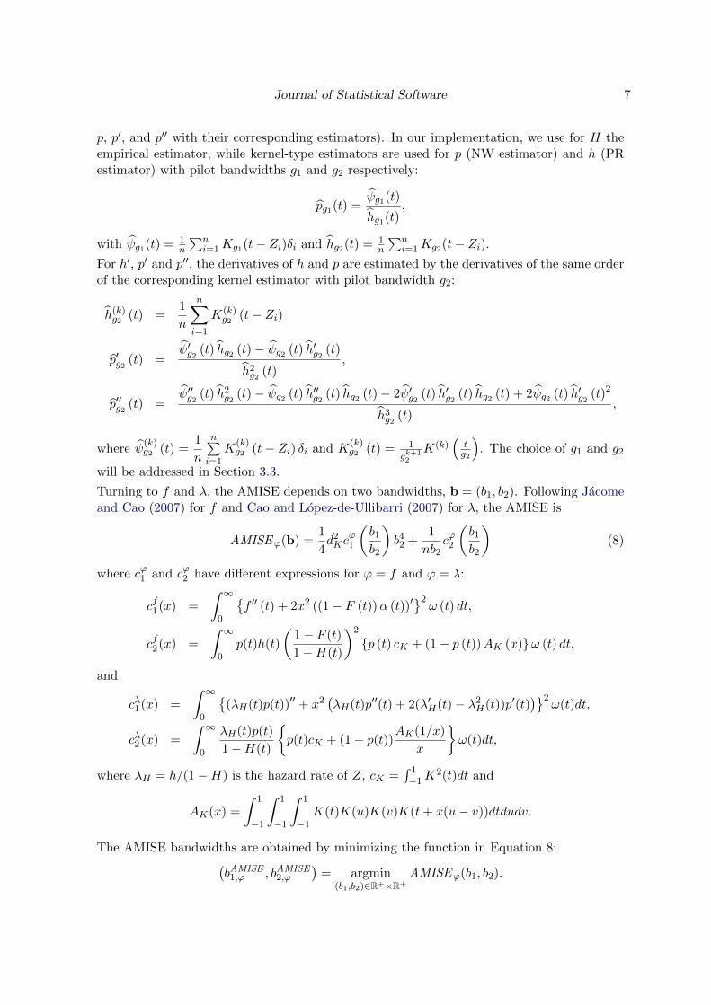
Journal of Statistical Software 7
p, p′, and p′′ with their corresponding estimators). In our implementation, we use for H theempirical estimator, while kernel-type estimators are used for p (NW estimator) and h (PRestimator) with pilot bandwidths g1 and g2 respectively:
pg1(t) =ψg1(t)
hg1(t),
with ψg1(t) = 1n
∑ni=1Kg1(t− Zi)δi and hg2(t) = 1
n
∑ni=1Kg2(t− Zi).
For h′, p′ and p′′, the derivatives of h and p are estimated by the derivatives of the same orderof the corresponding kernel estimator with pilot bandwidth g2:
h(k)g2 (t) =
1
n
n∑i=1
K(k)g2 (t− Zi)
p′g2 (t) =ψ′g2 (t) hg2 (t)− ψg2 (t) h′g2 (t)
h2g2 (t)
,
p′′g2 (t) =ψ′′g2 (t) h2
g2 (t)− ψg2 (t) h′′g2 (t) hg2 (t)− 2ψ′g2 (t) h′g2 (t) hg2 (t) + 2ψg2 (t) h′g2 (t)2
h3g2 (t)
,
where ψ(k)g2 (t) =
1
n
n∑i=1
K(k)g2 (t− Zi) δi and K
(k)g2 (t) = 1
gk+12
K(k)(tg2
). The choice of g1 and g2
will be addressed in Section 3.3.
Turning to f and λ, the AMISE depends on two bandwidths, b = (b1, b2). Following Jacomeand Cao (2007) for f and Cao and Lopez-de-Ullibarri (2007) for λ, the AMISE is
AMISEϕ(b) =1
4d2Kc
ϕ1
(b1b2
)b42 +
1
nb2cϕ2
(b1b2
)(8)
where cϕ1 and cϕ2 have different expressions for ϕ = f and ϕ = λ:
cf1(x) =
∫ ∞0
{f ′′ (t) + 2x2 ((1− F (t))α (t))′
}2ω (t) dt,
cf2(x) =
∫ ∞0
p(t)h(t)
(1− F (t)
1−H(t)
)2
{p (t) cK + (1− p (t))AK (x)}ω (t) dt,
and
cλ1(x) =
∫ ∞0
{(λH(t)p(t))′′ + x2
(λH(t)p′′(t) + 2(λ′H(t)− λ2
H(t))p′(t))}2
ω(t)dt,
cλ2(x) =
∫ ∞0
λH(t)p(t)
1−H(t)
{p(t)cK + (1− p(t))AK(1/x)
x
}ω(t)dt,
where λH = h/(1−H) is the hazard rate of Z, cK =∫ 1−1K
2(t)dt and
AK(x) =
∫ 1
−1
∫ 1
−1
∫ 1
−1K(t)K(u)K(v)K(t+ x(u− v))dtdudv.
The AMISE bandwidths are obtained by minimizing the function in Equation 8:(bAMISE1,ϕ , bAMISE
2,ϕ
)= argmin
(b1,b2)∈R+×R+
AMISEϕ(b1, b2).

8 survPresmooth: Presmoothed Estimation in Survival Analysis in R
It can be shown that without presmoothing (i.e., b1 = 0) thenAK(0) = limx→∞ x−1AK(1/x) =
cK . As a consequence, AMISEϕ reduces to that of the classical estimators of f and λ, and theminimization in b2 of AMISEϕ (0, b2) gives the well-known plug-in bandwidth for the classicalkernel estimates of f and λ (see Sanchez-Sellero, Gonzalez-Manteiga, and Cao 1999).
Again, the plug-in bandwidth selector for b = (b1, b2) requires some estimates of the functionsH, p, p′, p′′, h, h′, h′′, F and f ′′ (the last two only for ϕ = f) to be plugged-in into the termscϕ1 and cϕ2 of Equation 8 and proceeds by numerically minimizing the resulting estimate ofAMISEϕ. As before, our implementation makes use of the empirical estimator for H, the
NW estimator and derivatives with pilot bandwidth b1 for p, p′ and p′′, and the PR estimatorand derivatives with pilot bandwidth b3 for h, h′ and h′′. When ϕ = f , we estimate F and
f using the presmoothed estimators with bandwidths b = b1 and b =(b1, b2
)respectively.
Section 3.3 below explains the procedure we follow to choose the needed pilot bandwidthsb1, b2 and b3.
3.2. Bootstrap bandwidth selector
The bootstrap bandwidth selector for b is obtained by minimizing a bootstrap estimate ofthe MISE in Equation 6 according to the following algorithm:
1. Generate B bootstrap resamples {Z∗i , δ∗i }ni=1 from the original data {Zi, δi}ni=1. The
resampling method must be adapted to the censored data context. Here we use theprocedure called ‘presmoothed simple’ in Jacome et al. (2008), which, in general, exhibitsa good practical performance:
(a) Draw {Z∗i }ni=1 by sampling randomly with replacement from {Zi}ni=1.
(b) Draw {δ∗i }ni=1 from the conditional Bernoulli distribution with parameter p
b1(Z∗i ).
Here, pb1
(·) is the NW estimator of p computed with the pilot bandwidth b1 (seeSection 3.3 for pilot bandwidth selection).
2. For the jth bootstrap resample (j = 1, . . . , B), compute ϕP∗(j)bl
, the presmoothed esti-mator with bandwidth bl, l = 1, 2, . . . , L, in a grid of L bandwidths.
3. With the original sample {Zi, δi}ni=1 compute the presmoothed estimator ϕPb
using the
pilot bandwidth b (see Section 3.3 for pilot bandwidth selection).
4. Obtain the Monte Carlo approximation of the bootstrap version of MISE for eachbandwidth bl, l = 1, 2, . . . , L:
MISE ∗ϕ(bl) '1
B
B∑j=1
∫ ∞0
(ϕP∗(j)bl
(t)− ϕPb
(t))2ω (t) dt. (9)
5. The bootstrap bandwidth, b∗ϕ, is the minimizer of MISE ∗ϕ over the grid of bandwidths:
b∗ϕ = argminb∈{b1,b2,...,bL}
MISE ∗ϕ(b).

Journal of Statistical Software 9
3.3. Selection of the pilot bandwidths
As discussed above, both the bootstrap and plug-in methods require the preliminary compu-tation of some pilot bandwidths.
Plug-in bandwidth
When the estimand ϕ is S or Λ, the plug-in bandwidth selector of b = b1 is obtained byreplacing in Equation 7 the constants Q and A with the following estimates:
Qg1 =1
n
n∑i=1
pg1(Zi)(1− pg1(Zi))ω(Zi)
(1−Hn(Zi) + 1/n)2,
Ag2 =
∫ ∞0
α2g2(v)ω(v)dv with αg2(t) =
∫ t
0
12 p′′g2(u)hg2(u) + p′g2(u)h′g2(u)
1−Hn(u) + 1/ndu.
Theorems 7 and 8 of Cao et al. (2005) give expressions for the optimal pilot bandwidths g1
and g2, in the sense of minimizing the asymptotic MSE of Qg1 and Ag2 . These bandwidthsdepend on some unknown functions: p, H and their first four derivatives. At this stage, weestimate g1 and g2 parametrically by fitting a logistic regression model for p and assuming aWeibull model for H.
In the case of ϕ = f, λ, we choose the pilot bandwidths b1, b2 and b3 following the procedureadopted by Jacome (2005). Specifically, the first pilot bandwidth b1, used for the NW esti-mates of p and its derivatives, is obtained by cross-validation (see Stone 1974). When ϕ = f ,we use for F and f ′′ the corresponding presmoothed estimators with bandwidths b = b1 and
b =(b1, b2
)respectively, where:
b2 =
cK′′
n∑i=1
(1− FKMn (Zi)
1−Hn(Zi) + 1/n
)2
δiω(Zi)
ndK∫∞
0 f ′′′(t)2ω(t)dt
1/7
, (10)
with cK′′ =∫ 1−1K
′′(t)2dt. This expression for the bandwidth b2 is an estimate of the optimal
bandwidth for estimating the curvature∫∞
0 f ′′(t)2ω(t)dt under censoring (see Sanchez-Selleroet al. 1999). The estimation of f ′′′ in Equation 10 is not an easy matter. We use a parametric,but flexible, procedure, which fits a mixture of three Weibull distributions by maximumlikelihood.
Finally, to compute the PR estimates of h and its derivatives, we use another pilot bandwidthb3, which is essentially equivalent to b2 in a setting without censoring:
b3 =
(cK′′
ndK∫∞
0 h′′′(t)2ω(t)dt
)1/7
. (11)
The estimation of h′′′ in Equation 11 is carried out in a similar way to that of f ′′′ in Equa-tion 10.
10 survPresmooth: Presmoothed Estimation in Survival Analysis in R
Bootstrap bandwidth
If the estimands are S or Λ, one pilot bandwidth b1 is required to compute the NW estimatorpb1 and the presmoothed estimator in steps 1 and 3 of the algorithm described in Section 3.2.
On the other hand, when the estimands are f or λ a second bandwidth, b2 is required forcomputing ϕP
bin step 3 of the algorithm mentioned above.
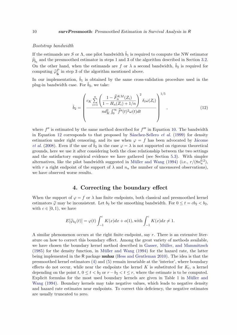
In our implementation, b1 is obtained by the same cross-validation procedure used in theplug-in bandwidth case. For b2, we take:
b2 =
cK
n∑i=1
(1− FKMn (Zi)
1−Hn(Zi) + 1/n
)2
δiω(Zi)
nd2K
∫∞0 f ′′(t)2ω(t)dt
1/5
, (12)
where f ′′ is estimated by the same method described for f ′′′ in Equation 10. The bandwidthin Equation 12 corresponds to that proposed by Sanchez-Sellero et al. (1999) for densityestimation under right censoring, and its use when ϕ = f has been advocated by Jacomeet al. (2008). Even if the use of b2 in the case ϕ = λ is not supported on rigorous theoreticalgrounds, here we use it after considering both the close relationship between the two settingsand the satisfactory empirical evidence we have gathered (see Section 5.3). With simpleralternatives, like the pilot bandwidth suggested in Muller and Wang (1994) (i.e., r/(8n0.2
u ),with r a right endpoint of the support of λ and nu the number of uncensored observations),we have observed worse results.
4. Correcting the boundary effect
When the support of ϕ = f or λ has finite endpoints, both classical and presmoothed kernelestimators ϕ may be inconsistent. Let b2 be the smoothing bandwidth. For 0 ≤ t = cb2 < b2,with c ∈ [0, 1), we have
E[ϕb2(t)] = ϕ(t)
∫ c
−1K(x)dx+ o(1),with
∫ c
−1K(x)dx 6= 1.
A similar phenomenon occurs at the right finite endpoint, say r. There is an extensive liter-ature on how to correct this boundary effect. Among the great variety of methods available,we have chosen the boundary kernel method described in Gasser, Muller, and Mammitzsch(1985) for the density function, in Muller and Wang (1994) for the hazard rate, the latterbeing implemented in the R package muhaz (Hess and Gentleman 2010). The idea is that thepresmoothed kernel estimators (4) and (5) remain invariable at the ‘interior’, where boundaryeffects do not occur, while near the endpoints the kernel K is substituted for Kt, a kerneldepending on the point t, 0 ≤ t < b2 or r− b2 < t ≤ r, where the estimate is to be computed.Explicit formulas for the most used boundary kernels are given in Table 1 in Muller andWang (1994). Boundary kernels may take negative values, which leads to negative densityand hazard rate estimates near endpoints. To correct this deficiency, the negative estimatesare usually truncated to zero.
Journal of Statistical Software 11
In our implementation the selected bandwidth b is the same independently of whether theboundary effect is corrected or not. This is justified by the fact that b is a global bandwidthchosen as the minimizer of the MISEϕ in Equation 6, where the weight function ω discardsthe boundary points.
5. The survPresmooth package
This section contains a brief description of the package functionality. This is followed by theresults of the analysis of a real dataset and a simulation study, both of them carried out withthe package.
5.1. General description
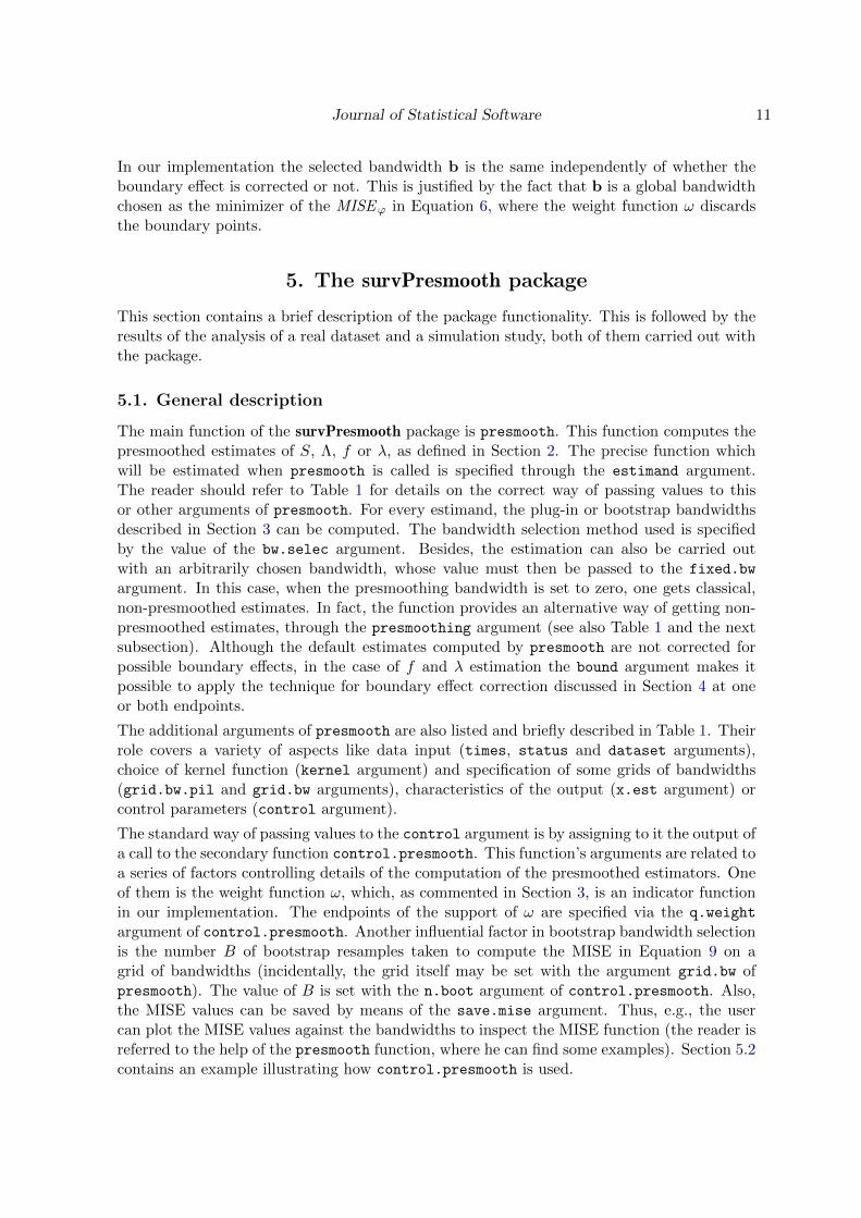
The main function of the survPresmooth package is presmooth. This function computes thepresmoothed estimates of S, Λ, f or λ, as defined in Section 2. The precise function whichwill be estimated when presmooth is called is specified through the estimand argument.The reader should refer to Table 1 for details on the correct way of passing values to thisor other arguments of presmooth. For every estimand, the plug-in or bootstrap bandwidthsdescribed in Section 3 can be computed. The bandwidth selection method used is specifiedby the value of the bw.selec argument. Besides, the estimation can also be carried outwith an arbitrarily chosen bandwidth, whose value must then be passed to the fixed.bw
argument. In this case, when the presmoothing bandwidth is set to zero, one gets classical,non-presmoothed estimates. In fact, the function provides an alternative way of getting non-presmoothed estimates, through the presmoothing argument (see also Table 1 and the nextsubsection). Although the default estimates computed by presmooth are not corrected forpossible boundary effects, in the case of f and λ estimation the bound argument makes itpossible to apply the technique for boundary effect correction discussed in Section 4 at oneor both endpoints.
The additional arguments of presmooth are also listed and briefly described in Table 1. Theirrole covers a variety of aspects like data input (times, status and dataset arguments),choice of kernel function (kernel argument) and specification of some grids of bandwidths(grid.bw.pil and grid.bw arguments), characteristics of the output (x.est argument) orcontrol parameters (control argument).
The standard way of passing values to the control argument is by assigning to it the output ofa call to the secondary function control.presmooth. This function’s arguments are related toa series of factors controlling details of the computation of the presmoothed estimators. Oneof them is the weight function ω, which, as commented in Section 3, is an indicator functionin our implementation. The endpoints of the support of ω are specified via the q.weight
argument of control.presmooth. Another influential factor in bootstrap bandwidth selectionis the number B of bootstrap resamples taken to compute the MISE in Equation 9 on agrid of bandwidths (incidentally, the grid itself may be set with the argument grid.bw ofpresmooth). The value of B is set with the n.boot argument of control.presmooth. Also,the MISE values can be saved by means of the save.mise argument. Thus, e.g., the usercan plot the MISE values against the bandwidths to inspect the MISE function (the reader isreferred to the help of the presmooth function, where he can find some examples). Section 5.2contains an example illustrating how control.presmooth is used.
12 survPresmooth: Presmoothed Estimation in Survival Analysis in R
Argument Description
times An object of mode numeric giving the observed times. If dataset is notNULL it is interpreted as the name of the corresponding variable of thedataset.
status An object of mode numeric giving the censoring status of the times codedin the times object. If dataset is not NULL it is interpreted as the nameof the corresponding variable of the dataset.
dataset A data frame in which the variables named in times and status are in-terpreted. If NULL, times and status must be objects of the workspace.
estimand A character string identifying the function to estimate: "S", the default,for S, "H" for Λ, "f" for f and "h" for λ.
bw.selec A character string specifying the bandwidth selection method: "fixed",the default, if no bandwidth selection is done, "plug-in" for plug-in band-width selection and "bootstrap" for bootstrap bandwidth selection.
presmoothing A logical value indicating if the presmoothed estimates (TRUE, the default)or their non-presmoothed counterparts (FALSE) will be computed.
fixed.bw A numeric vector with the fixed bandwidth(s) used when the value of thebw.selec argument is "fixed". It has length 1 for estimating S and Λ, or2 for f and λ (then, the first element is the presmoothing bandwidth b1).
grid.bw.pil A numeric vector specifying the grid where the presmoothing pilot band-width will be selected using the cross-validation method. Not used inplug-in bandwidth selection for S or Λ estimation.
grid.bw A list of length 1 (for S or Λ estimation) or 2 (for f and λ estimation)whose component(s) is (are) a (two) numeric vector(s) specifying the gridof bandwidths needed for bootstrap bandwidth selection when the valueof the bw.selec argument is "bootstrap". For S or Λ estimation, it canalso be a numeric vector.
kernel A character string specifying the kernel function used. One of "biweight",for biweight kernel (the default), and "triweight", for triweight kernel.
bound A character string specifying the end(s) of the data range where boundarycorrection is applied. If "none", the default, no correction is done; if"left", "right" or "both", the correction is applied at the left, right orboth ends.
x.est A numeric vector specifying the points where the estimate is computed.control A list of control values. The default value is the output returned by the
control.presmooth function called without arguments.
Table 1: Arguments of the presmooth function and their description.
The output produced by presmooth is a list of class survPresmooth. The package implementsa method for printing objects of this class, which by default (i.e., when the object name is en-tered in the command line) performs only a minimal formatting of the output. In Section 5.2,an example showing how to call explicitly the print method is given.
From a computational point of view, although R is the programming environment for thepackage, for efficiency reasons the main function (i.e., presmooth) makes extensive use ofcompiled C code.

Journal of Statistical Software 13
5.2. Application to a real dataset
Here we present an analysis of a dataset taken from Klein and Moeschberger (2003). This is thealloauto dataset included as part of the R package KMsurv (Klein, Moeschberger, and Yan2012). It collects information about a sample of 101 patients with acute myelogenous leukemiareported to the International Bone Marrow Transplant Registry. All patients received a bonemarrow transplantation, but they may differ with respect to its type: allogeneic (ALLO)or autologous (AUTO). It should be clear that our purpose when analyzing this dataset isonly to illustrate the functionality of the package through a real example, not to answer anysubstantive questions about the data itself.
In this dataset, event (i.e., death or relapse) times may be right censored by end of follow-up.The incidence of censoring is moderate (50.5%), slightly higher in the ALLO group (56.0%)than in the AUTO group (45.1%). The variables in data frame alloauto are: time, thetime (months) to death or relapse; delta, an indicator of death or relapse (0 = alive withoutrelapse, 1 = death or relapse); and type, the type of transplant (1 = ALLO, 2 = AUTO). Atotal of 50 patients had ALLO and 51 AUTO transplants.
Before starting our analysis, we create one separate R object for each group of patients.
R> library("KMsurv")
R> data("alloauto")
R> allo <- alloauto[alloauto$type == 1, c("time", "delta")]
R> auto <- alloauto[alloauto$type == 2, c("time", "delta")]
Next, it is shown how to use the presmooth function to obtain estimates of the functions thatcharacterize the survival time for each of the two groups defined by type of transplant:
R> library("survPresmooth")
R> allo.S.pi <- presmooth(times = time, status = delta, dataset = allo,
+ estimand = "S", bw.selec = "plug-in")
R> allo.H.pi <- presmooth(time, delta, allo, "H", "plug-in")
R> allo.S.boot <- presmooth(time, delta, allo, "S", "bootstrap")
R> allo.H.boot <- presmooth(time, delta, allo, "H", "bootstrap")
R> auto.S.pi <- presmooth(time, delta, auto, "S", "plug-in")
R> auto.H.pi <- presmooth(time, delta, auto, "H", "plug-in")
R> auto.S.boot <- presmooth(time, delta, auto, "S", "bootstrap")
R> auto.H.boot <- presmooth(time, delta, auto, "H", "bootstrap")
As can be seen from the code, the identity of the curve which is estimated and the bandwidthselection method used are determined by the values passed to the estimand and bw.selec
arguments, respectively. Let us point out that the program sets an upper bound equal to therange of the observed times for any selected bandwidth.
For comparison reasons, it is interesting to obtain the KM and NA estimates for the twogroups of patients. As mentioned before, these classical estimators are recovered from thecorresponding presmoothed estimators when the presmoothing bandwidth b1 is zero. With thepresmooth function this can be done by setting the bw.selec argument to "fixed" (actually,this is the default value) and the fixed.bw argument to 0:

14 survPresmooth: Presmoothed Estimation in Survival Analysis in R
Presmoothing bandwidth b1 Smoothing bandwidth b2
Group Estimand Plug-in Bootstrap Plug-in Bootstrap
ALLO S,Λ 4.51 6.06 – –f 8.46 8.56 6.63 (6.87) 10.78λ 7.59 6.06 3.91 (4.41) 12.09
AUTO S,Λ 17.53 7.83 – –f 12.26 11.06 13.89 (14.05) 22.07λ 14.60 9.86 12.05 (11.96) 24.76
Table 2: Selected bandwidths for the alloauto dataset. The bandwidths between parenthesescorrespond to the non-presmoothed estimates shown in Figure 2 (see text for details).
R> allo.km <- presmooth(time, delta, allo, "S", "fixed", fixed.bw = 0)
R> allo.na <- presmooth(time, delta, allo, "H", "fixed", fixed.bw = 0)
R> auto.km <- presmooth(time, delta, auto, "S", "fixed", fixed.bw = 0)
R> auto.na <- presmooth(time, delta, auto, "H", "fixed", fixed.bw = 0)
An alternative method of obtaining these non-presmoothed estimates consists in passing thevalue FALSE to the argument presmoothing. For example, allo.km could also be computedby
R> presmooth(time, delta, allo, "S", presmoothing = FALSE)
Figure 1 is a plot of the estimates of the S and Λ functions. It is easily drawn from the objectscreated by the previous code (i.e., from the information contained in their components x.estand estimate), by using R’s basic plotting facilities. For example, the top left panel isproduced by executing:
R> plot(allo.S.pi$x.est, allo.S.pi$estimate, type = "s", xlab = "Time",
+ ylab = "Survival", ylim = c(0, 1), main = "Allogeneic transplant",
+ col = "blue")
R> lines(allo.S.boot$x.est, allo.S.boot$estimate, type = "s", col = "red")
R> lines(allo.km$x.est, allo.km$estimate, type = "s", lty = "dotted")
A general comparison of the different estimates of Figure 1 reveals mainly minor small-scaledifferences. As expected, the presmoothed estimates are characterized by jumps that aresmaller and more frequent than in the corresponding empirical estimates. This reflects thefact that the presmoothed estimates carry more information on the local behavior of thelifetime distribution. Only in the case of the AUTO group with plug-in bandwidth, striking,large-scale differences affecting the right tail of the estimates are observed. Of course, allthese facts are determined by the specific values of the bandwidths, which are collected inTable 2.
The selected bandwidths are saved in the bandwidth component of the objects of classsurvPresmooth. They are printed by default by the print method for objects of the class. Ifa formatted output including other components of the survPresmooth object is needed, theprint.survPresmooth function must be explicitly called, with the name of the component(s)assigned to the more argument. For example, to print the pilot bandwidths:

Journal of Statistical Software 15
0 10 20 30 40 50 60
0.0
0.2
0.4
0.6
0.8
1.0
Allogeneic transplant
Time
Sur
viva
l
0 10 20 30 40 50
0.0
0.2
0.4
0.6
0.8
1.0
Autologous transplant
TimeS
urvi
val
0 10 20 30 40 50 60
0.0
0.1
0.2
0.3
0.4
0.5
0.6
Allogeneic transplant
Time
Cum
ulat
ive
haza
rd
0 10 20 30 40 50
0.0
0.5
1.0
1.5
Autologous transplant
Time
Cum
ulat
ive
haza
rd
Figure 1: alloauto dataset. Estimates of S (top panels) and Λ (bottom panels), conditionedby type of transplant. The presmoothed estimates were obtained with either plug-in (bluelines) or bootstrap (red lines) bandwidth selection. Also shown are the KM and NA estimatesof S and Λ, respectively (dotted black lines).
R> print(allo.S.pi, more = "pilot.bw")
Presmoothed estimation of the survival function, S(t)
t S(t)
1 0.030 0.9800045
2 0.493 0.9601144
....

16 survPresmooth: Presmoothed Estimation in Survival Analysis in R
49 58.322 0.5208789
50 60.625 0.5208789
Bandwidth selection method: plug-in
Bandwidth(s):
presmoothing: 4.510372
Pilot bandwidth(s):
[1] 5.612775 8.989902
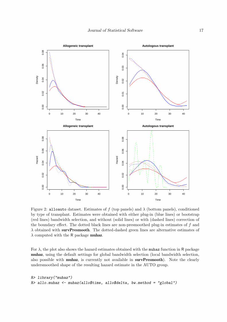
As for the f and λ functions, Figure 2 provides a plot of their presmoothed estimates. Theselected plug-in and bootstrap bandwidths are also collected in Table 2. The bootstrap selec-tor seems to give slightly large smoothing bandwidths b2, which entails smoother estimationsthan those with the plug-in bandwidth selection. We also show how the estimates changedepending on whether the boundary effect is corrected or not.
Here we only give details on the R code run to get the estimates displayed on Figure 2 for thecase of f estimation in the ALLO group:
R> allo.f.pi <- presmooth(time, delta, allo, "f", "plug-in")
R> allo.f.boot <- presmooth(time, delta, allo, "f", "bootstrap")
R> allo.f.pi.bound <- presmooth(time, delta, allo, "f", "plug-in",
+ bound = "both")
R> allo.f.boot.bound <- presmooth(time, delta, allo, "f", "bootstrap",
+ bound = "both")
The estimates are computed at the points given by the x.est argument (see Table 1). When,as in the previous lines of code, its value is not explicitly set, presmooth computes it internally.With the default value of x.est, estimation is done at a sequence of 50 equispaced pointsbetween the minimum and the 90th percentile of the observed times. As a guideline, densityand hazard estimates at the right tail should be taken very cautiously due to their increasedbias and variance.
A warning should be given about computing time, which is usually markedly longer for boot-strap than for plug-in bandwidth selection. Of course, this difference is due to the computer-intensive nature of bootstrap methods. On a machine with an Intel Core i7-3610QM processorand 7.7 GB of memory, the last two lines of code took respectively 3.372 and 14.857 secondsof CPU time.
Our bandwidth selectors for f and λ can be extended to the case without presmoothing,allowing the selection of plug-in and bootstrap smoothing bandwidths for the correspond-ing classical kernel estimators of these curves. For reference, the classical non-presmoothedestimates of f and λ thus obtained (with plug-in bandwidth selection) have been added toFigure 2 (and the values of the corresponding bandwidths to Table 2). For f , this estimateis computed by:
R> allo.f.pi.np <- presmooth(time, delta, allo, "f", "plug-in",
+ presmoothing = FALSE)
Journal of Statistical Software 17
0 10 20 30 40
0.00
0.02
0.04
0.06
0.08
Allogeneic transplant
Time
Den
sity
0 10 20 30 40
0.00
0.01
0.02
0.03
0.04
Autologous transplant
TimeD
ensi
ty
0 10 20 30 40
0.00
0.02
0.04
0.06
0.08
Allogeneic transplant
Time
Haz
ard
0 10 20 30 40
0.00
0.02
0.04
0.06
0.08
Autologous transplant
Time
Haz
ard
Figure 2: alloauto dataset. Estimates of f (top panels) and λ (bottom panels), conditionedby type of transplant. Estimates were obtained with either plug-in (blue lines) or bootstrap(red lines) bandwidth selection, and without (solid lines) or with (dashed lines) correction ofthe boundary effect. The dotted black lines are non-presmoothed plug-in estimates of f andλ obtained with survPresmooth. The dotted-dashed green lines are alternative estimates ofλ computed with the R package muhaz.
For λ, the plot also shows the hazard estimates obtained with the muhaz function in R packagemuhaz, using the default settings for global bandwidth selection (local bandwidth selection,also possible with muhaz, is currently not available in survPresmooth). Note the clearlyundersmoothed shape of the resulting hazard estimate in the AUTO group.
R> library("muhaz")
R> allo.muhaz <- muhaz(allo$time, allo$delta, bw.method = "global")
18 survPresmooth: Presmoothed Estimation in Survival Analysis in R
T C
Model αT βT αC βC π
I 1 4 1 5 0.48II 1 0.7 0.25 0.9 0.73III 1 4 0.8 4 0.71
Table 3: Characteristics of the simulated models I , II and III .
Further aspects of the computation of the presmoothed estimates of S, Λ, f or λ can befine-tuned by means of other arguments, including the control argument and the associatedcontrol.presmooth function. For example, the following code would compute the pres-moothed estimate of S for the AUTO group with bootstrap bandwidth selected from a gridof 150 equispaced bandwidths between 1 and 50, taking B = 10000 bootstrap resamples, anda weight function with support on the interval defined by the 10th and 90th percentiles of theobserved times:
R> presmooth(time, delta, auto, "S", "bootstrap",
+ grid.bw = seq(1, 50, length.out = 150),
+ control = control.presmooth(n.boot = 10000, q.weight = c(0.1, 0.9)))
5.3. Simulations
The practical performance of the presmoothed estimators and bandwidth selectors imple-mented in survPresmooth may be shown by means of simulation experiments. We havesimulated four different models in order to describe the behavior in (non-cumulative and cu-mulative) hazard function estimation with varying sample size. For the sake of brevity, wedo not give any results for survival and density functions. The models we have simulatedtry to define scenarios showing different combinations of purportedly influential conditions,like the intensity of censoring, the constant or non-constant nature of the p function, and theincreasing, decreasing or non-monotonic nature of the hazard function.
In models I , II and III , both survival and censoring times follow a Weibull distribution withhazard function:
λ(t) =β
α
(t
α
)β−1
, t > 0,
where α and β are the scale and shape parameters.
The parameters characterizing the survival and censoring times of these models are collectedin Table 3. Also shown is the value of the unconditional probability of censoring π = 1 −∫∞
0 p(t)h(t)dt, where h is the density of Z.
For model IV we have considered the distribution proposed by Chen (2000). For parametersα > 0, β > 0, Chen’s hazard function is
λ(t) = αβtβ−1 exp(tβ), t > 0.
It can be shown that λ has a bathtub shape for β < 1 and it is an increasing function for β ≥ 1(Chen 2000). In model IV , the survival and censoring times have Chen distributions with
Journal of Statistical Software 19
Model I
t
0.0 0.2 0.4 0.6 0.8 1.0
0.4
0.5
0.6
0.7
0.8
0.9
1.0
p(t)
01
23
4
λ(t)
Model II
t
0.00 0.10 0.20 0.30 0.40
0.20
0.24
0.28
0.32
0.36
0.40
p(t)
1.0
1.5
2.0
2.5
λ(t)
Model III
t
0.0 0.1 0.2 0.3 0.4 0.5 0.6 0.7 0.8 0.9
0.20
0.25
0.30
0.35
0.40
p(t)
01
23
4
λ(t)
Model IV
t
0.0 0.1 0.2 0.3 0.4 0.5 0.6 0.7
0.4
0.5
0.6
0.7
0.8
0.9
p(t)
1.6
1.8
2.0
2.2
2.4
2.6
2.8
λ(t)
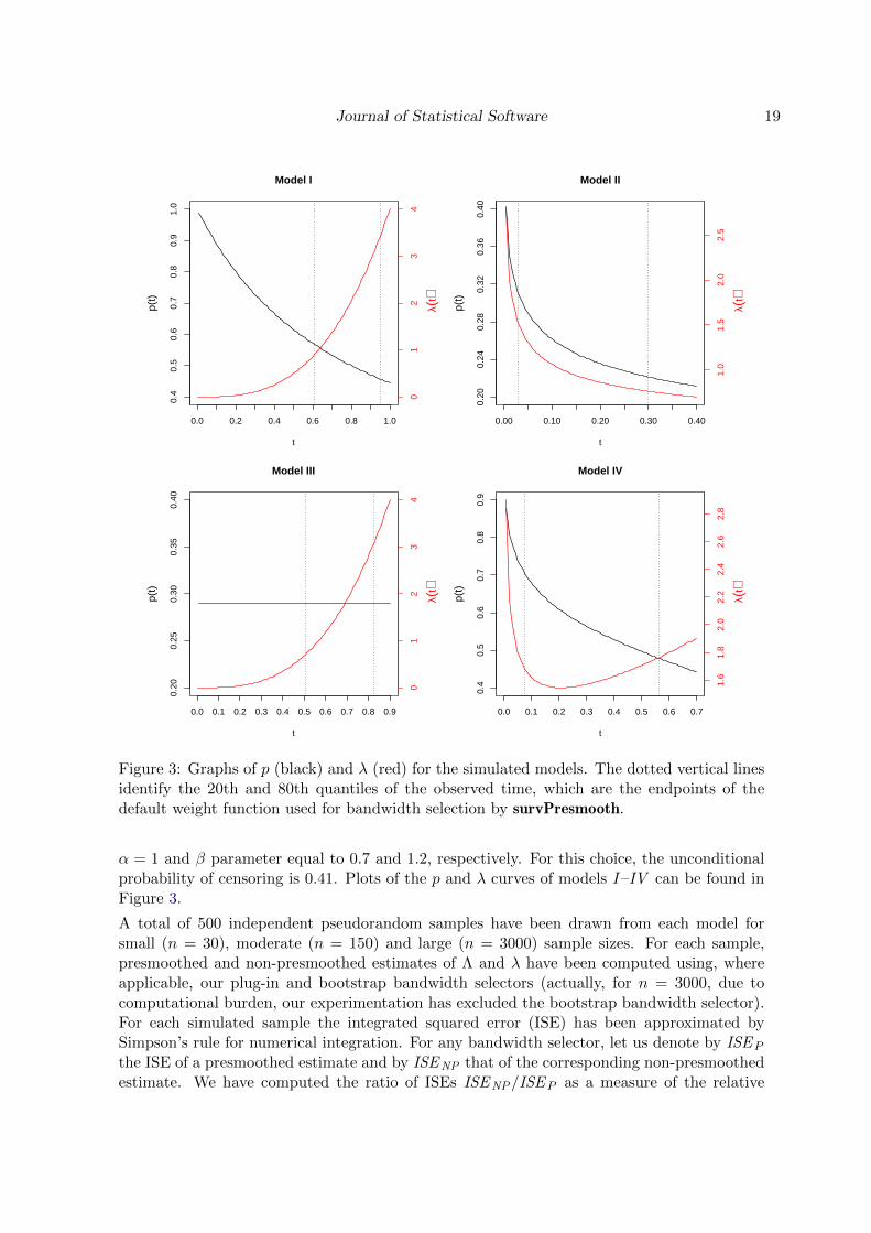
Figure 3: Graphs of p (black) and λ (red) for the simulated models. The dotted vertical linesidentify the 20th and 80th quantiles of the observed time, which are the endpoints of thedefault weight function used for bandwidth selection by survPresmooth.
α = 1 and β parameter equal to 0.7 and 1.2, respectively. For this choice, the unconditionalprobability of censoring is 0.41. Plots of the p and λ curves of models I –IV can be found inFigure 3.
A total of 500 independent pseudorandom samples have been drawn from each model forsmall (n = 30), moderate (n = 150) and large (n = 3000) sample sizes. For each sample,presmoothed and non-presmoothed estimates of Λ and λ have been computed using, whereapplicable, our plug-in and bootstrap bandwidth selectors (actually, for n = 3000, due tocomputational burden, our experimentation has excluded the bootstrap bandwidth selector).For each simulated sample the integrated squared error (ISE) has been approximated bySimpson’s rule for numerical integration. For any bandwidth selector, let us denote by ISEP
the ISE of a presmoothed estimate and by ISENP that of the corresponding non-presmoothedestimate. We have computed the ratio of ISEs ISENP/ISEP as a measure of the relative

20 survPresmooth: Presmoothed Estimation in Survival Analysis in R
0.5
1.0
2.0
5.0
10.0
Model I
Bandwidth selection method
ISE
rat
io
0.5
1.0
2.0
5.0
10.0
PI BOOT
0.2
0.5
1.0
2.0
5.0
10.0
Model II
Bandwidth selection method
ISE
rat
io
0.2
0.5
1.0
2.0
5.0
10.0
PI BOOT
0.1
0.2
0.5
1.0
2.0
5.0
10.0
Model III
Bandwidth selection method
ISE
rat
io
0.1
0.2
0.5
1.0
2.0
5.0
10.0
PI BOOT
0.2
0.5
1.0
2.0
5.0
Model IV
Bandwidth selection method
ISE
rat
io
0.2
0.5
1.0
2.0
5.0
PI BOOT
n = 30 n = 150 n = 3000
Figure 4: Simulation results: box plots of the ISENP/ISEP ratios for the non-presmoothedand presmoothed estimates of Λ (for notation, see text). PI: plug-in bandwidth; BOOT:bootstrap bandwidth.
efficiency of presmoothed and non-presmoothed estimators. When ISENP/ISEP takes a value,say r, greater than 1, presmoothing is more efficient for that sample; more specifically, thepresmoothed estimator is then r times more efficient than the non-presmothed one.
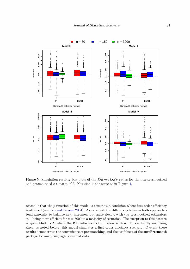
The box plots of the sampling distributions of the ISE ratios under the different simulatedscenarios are shown in Figure 4 for the case of Λ estimation, and in Figure 5 for λ. In theseplots, a logarithm scale has been used to facilitate comparison. The numerical values of themedians of the ISE ratios have been collected in Table 4. It is observed that, whatever thebandwidth selector chosen, for most of the simulated scenarios the presmoothed estimatorsare more efficient than the non-presmoothed ones. This is more striking for Model III ; the
Journal of Statistical Software 21
0.05
0.20
1.00
5.00
20.0
0
Model I
Bandwidth selection method
ISE
rat
io
0.05
0.20
1.00
5.00
20.0
0
PI BOOT
0.2
0.5
1.0
2.0
5.0
10.0
Model II
Bandwidth selection method
ISE
rat
io
0.2
0.5
1.0
2.0
5.0
10.0
PI BOOT
Model III
Bandwidth selection method
ISE
rat
io
PI BOOT
0.01
0.10
1.00
10.0
010
0.00
0.2
0.5
1.0
2.0
5.0
10.0
Model IV
Bandwidth selection method
ISE
rat
io
0.2
0.5
1.0
2.0
5.0
10.0
PI BOOT
n = 30 n = 150 n = 3000
Figure 5: Simulation results: box plots of the ISENP/ISEP ratios for the non-presmoothedand presmoothed estimates of λ. Notation is the same as in Figure 4.
reason is that the p function of this model is constant, a condition where first order efficiencyis attained (see Cao and Jacome 2004). As expected, the differences between both approachestend generally to balance as n increases, but quite slowly, with the presmoothed estimatorsstill being more efficient for n = 3000 in a majority of scenarios. The exception to this patternis again Model III , where the ISE ratio seems to increase with n. This is hardly surprisingsince, as noted before, this model simulates a first order efficiency scenario. Overall, theseresults demonstrate the convenience of presmoothing, and the usefulness of the survPresmoothpackage for analyzing right censored data.

22 survPresmooth: Presmoothed Estimation in Survival Analysis in R
Plug-in Bootstrap
Estimand Model n = 30 n = 150 n = 3000 n = 30 n = 150
Λ I 1.180 1.172 1.151 1.156 1.149II 1.119 1.078 1.009 1.199 1.135III 1.538 1.621 1.766 1.498 1.610IV 1.051 1.056 1.031 1.049 1.028
λ I 1.049 1.014 1.021 1.216 1.057II 1.125 1.280 1.077 1.075 1.194III 1.261 1.227 1.542 1.528 1.186IV 1.050 1.042 0.998 1.082 0.977
Table 4: Simulation results: medians of the ISENP/ISEP ratios for the non-presmoothed andpresmoothed estimates of Λ and λ (for notation, see text).
6. Conclusions
This paper deals mainly with the implementation in R of the presmoothed estimators of thesurvival, density, and cumulative and non-cumulative hazard functions of a right-censoredlifetime. The new R package survPresmooth is introduced and described. Also, the theoryunderlying presmoothing has been summarized and further evidence showing the advantagesof presmoothed estimators over their classical counterparts has been provided. The presmoothfunction of the package computes the presmoothed estimators in a user-friendly way. Thefunction also implements two different methods for computing of the required bandwidths,based on bootstrap and plug-in techniques. Additionally, our software allows to compute well-known classical, non-presmoothed estimators (including, where applicable, their bandwidths),which may be interpreted as particular cases of presmoothed estimators.
There are several topics that are not dealt with by our package. We close the discussion withan enumeration of some of these issues, which give the opportunity for future developmentsof the package.
Although initially the graphical comparison of two or more distributions (straightforwardlydone with survPresmooth) may be enough, hypothesis testing of the equality of survivaldistributions is more satisfactory from a statistical point of view. It is possible to adapt thelog-rank test and, in general, all the weighted tests in the literature to the use of presmoothedestimators. However, these “presmoothed tests” remain largely unexplored and they shouldbe carefully worked out before being implemented.
Our package does not provide confidence bands for the estimated functions. A way of con-structing them could be based on the bootstrap. The same resampling plan used for bootstrapbandwidth selection could be applied in order to compute the percentiles of the bootstrap dis-tribution of the estimates. The limits of pointwise confidence intervals could be constructedfrom these percentiles.
Sometimes, in addition to right censoring (RC), lifetimes are also subject to left trunca-tion (LT). The good properties of presmoothing are conserved in the so-called LTRC model:see Jacome and Iglesias-Perez (2008) for the case of S and Λ estimation, and Jacome andIglesias-Perez (2010) for f . This suggests that, in principe, the procedures implemented insurPresmooth could also be extended to include LTRC data.
Journal of Statistical Software 23
Another issue not considered in survPresmooth is the possible presence of covariates. Pres-moothing ideas are relatively new, and though survival analysis adjusting for covariates isof great interest, it has been scarcely investigated in the context of presmoothed estima-tion. For a semiparametric approach see de Una-Alvarez and Rodrıguez-Campos (2004) andIglesias-Perez and de Una-Alvarez (2008).
Finally, let us point out that the properties of presmoothed estimators have been studiedonly in the setting of independent data, but in some studies survival times may be depen-dent. Under rather weak conditions for dependence, the KM estimator is still consistent andasymptotically normal (Ying and Wei 1994; Cai 1998). Similar ideas could be applied to tryto prove that properties regarding consistency and asymptotic normality of the presmoothedestimators are also valid under the same weak conditions for dependence.
Acknowledgments
This research has been partially supported by the Spanish Ministry of Science and Innovation(Grant MTM2011-22392).
References
Aalen OO (1978). “Nonparametric Inference for a Family of Counting Processes.” The Annalsof Statistics, 6, 701–726.
Cai Z (1998). “Asymptotic Properties of Kaplan-Meier Estimator for Censored DependentData.” Statistics & Probability Letters, 37, 381–389.
Cao R, Jacome MA (2004). “Presmoothed Kernel Density Estimator for Censored Data.”Journal of Nonparametric Statistics, 16, 289–309.
Cao R, Lopez-de-Ullibarri I (2007). “Product-Type and Presmoothed Hazard Rate Estimatorswith Censored Data.” Test, 16, 355–382.
Cao R, Lopez-de-Ullibarri I, Janssen P, Veraverbeke N (2005). “Presmoothed Kaplan-Meierand Nelson-Aalen Estimators.” Journal of Nonparametric Statistics, 17, 31–56.
Chen Z (2000). “A New Two-Parameter Lifetime Distribution with Bathtub Shape or In-creasing Failure Rate Function.” Statistics & Probability Letters, 49, 155–161.
de Una-Alvarez J, Rodrıguez-Campos MC (2004). “Strong Consistency of PresmoothedKaplan-Meier Integrals when Covariables Are Present.” Statistics, 38, 483–496.
Dikta G (1998). “On Semiparametric Random Censorship Models.” Journal of StatisticalPlanning and Inference, 66, 253–279.
Dikta G (2000). “The Strong Law under Semiparametric Random Censorship Models.” Jour-nal of Statistical Planning and Inference, 83, 1–10.
Dikta G (2001). “Weak Representation of the Cumulative Hazard Function under Semipara-metric Censorship Models.” Statistics, 35, 395–409.

24 survPresmooth: Presmoothed Estimation in Survival Analysis in R
Foldes A, Rejto L, Winter BB (1981). “Strong Consistency Properties of Nonparametric Esti-mators for Randomly Censored Data. II Estimation of Density and Failure Rate.” PeriodicaMathematica Hungarica, 12, 15–29.
Gasser T, Muller HG (1979). “Kernel Estimation of Regression Functions.” In T Gasser,M Rosenblatt (eds.), Smoothing Techniques for Curve Estimation, volume 757 of LectureNotes in Mathematics, pp. 23–68. Springer-Verlag.
Gasser T, Muller HG, Mammitzsch V (1985). “Kernels for Nonparametric Curve Estimation.”Journal of the Royal Statistical Society B, 47, 238–252.
Hess K, Gentleman R (2010). muhaz: Hazard Function Estimation in Survival Analysis. Rpackage version 1.2.5, URL http://CRAN.R-project.org/package=muhaz.
Iglesias-Perez MC, de Una-Alvarez J (2008). “Nonparametric Estimation of the ConditionalDistribution Function in a Semiparametric Censorship Model.” Journal of Statistical Plan-ning and Inference, 138, 3044–3058.
Jacome MA (2005). Estimacion Presuavizada de las Funciones de Densidad y Distribucioncon Datos Censurados. Ph.D. thesis, Universidade da Coruna.
Jacome MA, Cao R (2007). “Almost Sure Asymptotic Representation for the PresmoothedDistribution and Density Estimators for Censored Data.” Statistics, 41, 517–534.
Jacome MA, Cao R (2008). “Strong Representation of the Presmoothed Quantile FunctionEstimator for Censored Data.” Statistica Neerlandica, 62, 425–440.
Jacome MA, Gijbels I, Cao R (2008). “Comparison of Presmoothing Methods in KernelDensity Estimation under Censoring.” Computational Statistics, 23, 381–406.
Jacome MA, Iglesias-Perez MC (2008). “Presmoothed Estimation with Left-Truncated andRight-Censored Data.” Communications in Statistics – Theory and Methods, 37, 2964–2983.
Jacome MA, Iglesias-Perez MC (2010). “Presmoothed Estimation of the Density Functionwith Truncated and Censored data.” Statistics, 44, 217–234.
Kaplan EL, Meier P (1958). “Nonparametric Estimation from Incomplete Observations.”Journal of the American Statistical Association, 53, 457–481.
Klein JP, Moeschberger ML (2003). Survival Analysis: Techniques for Censored and Trun-cated Data. Springer-Verlag.
Klein JP, Moeschberger ML, Yan J (2012). KMsurv: Data Sets from Klein and Moeschberger(1997), Survival Analysis. R package version 0.1-5, URL http://CRAN.R-project.org/
package=KMsurv.
Lopez-de-Ullibarri I, Jacome MA (2013). survPresmooth: Presmoothed Estimation in Sur-vival Analysis. R package version 1.1-8, URL http://CRAN.R-project.org/package=
survPresmooth.
Muller HG, Wang JL (1994). “Hazard Rate Estimation under Random Censoring with VaryingKernels and Bandwidths.” Biometrics, 50, 61–76.

Journal of Statistical Software 25
Nadaraya EA (1964). “On Estimating Regression.” Theory of Probability and Its Applications,10, 186–190.
Nelson W (1972). “Theory and Applications of Hazard Plotting for Censored Failure Data.”Technometrics, 14, 945–965.
Parzen E (1962). “On Estimation of a Probability Density Function and Mode.” The Annalsof Mathematical Statistics, 33, 1065–1076.
Ramlau-Hansen H (1983). “Smoothing Counting Process Intensities by Means of KernelFunctions.” The Annals of Statistics, 11, 453–466.
R Core Team (2013). R: A Language and Environment for Statistical Computing. R Founda-tion for Statistical Computing, Vienna, Austria. URL http://www.R-project.org/.
Rosenblatt M (1956). “Remarks on Some Nonparametric Estimates of a Density Function.”The Annals of Mathematical Statistics, 27, 832–837.
Sanchez-Sellero C, Gonzalez-Manteiga W, Cao R (1999). “Bandwidth Selection in DensityEstimation with Truncated and Censored Data.” Annals of the Institute of StatisticalMathematics, 51, 51–70.
Stone M (1974). “Cross-Validatory Choice and Assessment of Statistical Predictions.” Journalof the Royal Statistical Society B, 36, 111–147.
Tanner MA, Wong WH (1983). “The Estimation of the Hazard Function from RandomlyCensored Data by the Kernel Method.” The Annals of Statistics, 11, 989–993.
Watson GS (1964). “Smooth Regression Analysis.” Shankya A, 26, 359–372.
Yandell BS (1983). “Nonparametric Inference for Rates with Censored Data.” The Annals ofStatistics, 11, 1119–1135.
Ying Z, Wei LJ (1994). “The Kaplan-Meier Estimate for Dependent Failure Time Observa-tions.” Journal of Multivariate Analysis, 50, 17–29.
Affiliation:
Ignacio Lopez-de-UllibarriDepartamento de MatematicasUniversidade da CorunaEscuela Universitaria PolitecnicaFerrol, A Coruna, SpainE-mail: [email protected]

26 survPresmooth: Presmoothed Estimation in Survival Analysis in R
M. Amalia JacomeDepartamento de MatematicasUniversidade da CorunaFacultad de CienciasA Coruna, SpainE-mail: [email protected]
Journal of Statistical Software http://www.jstatsoft.org/
published by the American Statistical Association http://www.amstat.org/
Volume 54, Issue 11 Submitted: 2011-03-21August 2013 Accepted: 2013-03-13
Related Documents