Survival Analysis: Weeks 1-2 - Stanford Universityweb.stanford.edu/~lutian/coursepdf/survweek1.pdf · In survival analysis the exponential distribution is the ... observe the first

1

Survival Analysis: Weeks 1-2

Lu Tian and Richard Olshen

Stanford University

2

Survival Time/Failure Time/Event Time

• What is the survival outcomes? the time to a clinical event of

interest: terminal and non-terminal events.

1. the time from diagnosis of cancer to death

2. the time between administration of a vaccine and infection

date

3. the time from the initiation of a treatment to the time of

the disease progression.

3

Survival time T

• Let T be a nonnegative random variable denoting the time to

the event of interest (survival time/event time/failure time).

• The distribution of T could be discrete, continuous or a

mixture of both. We will focus on the continuous distribution.

4

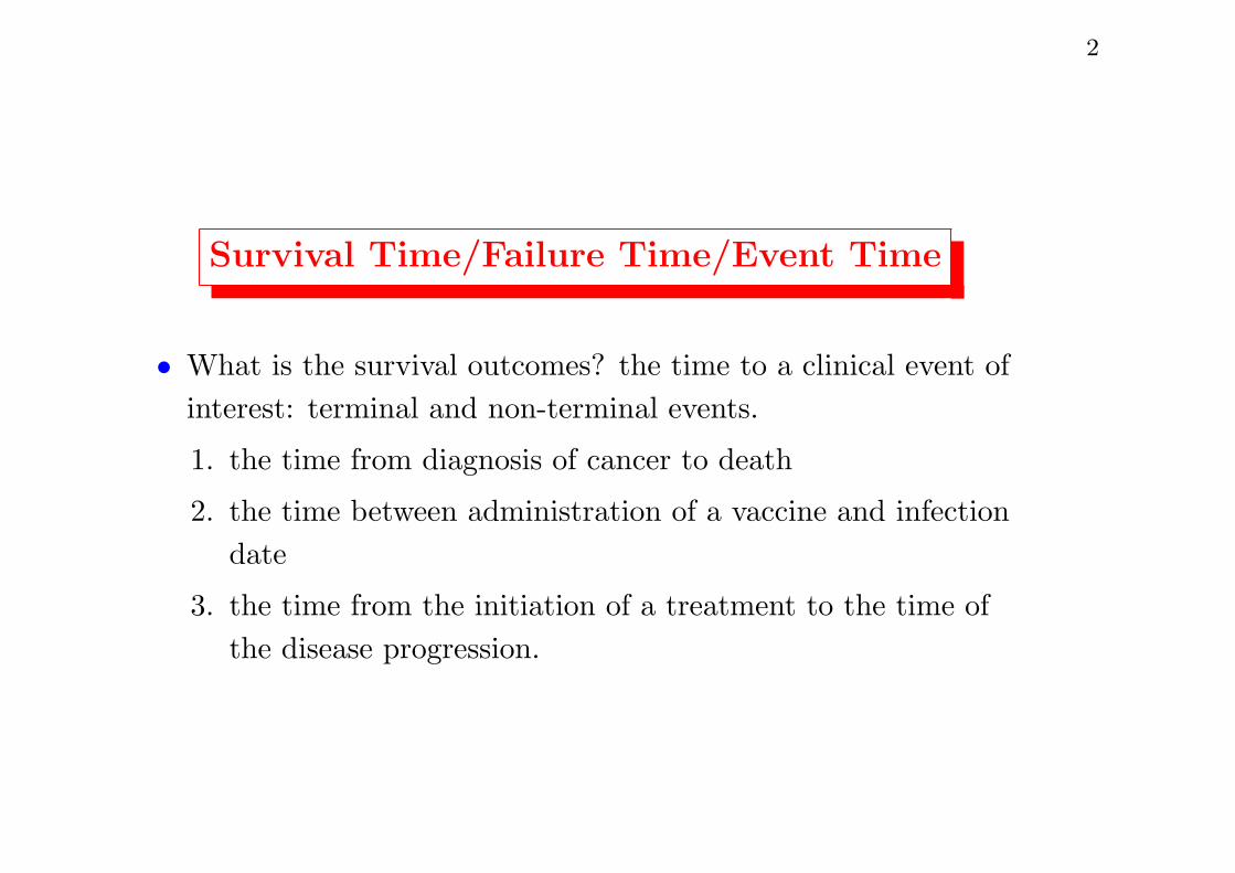
Survival time T

• The distribution of a random variable T ≥ 0 can be

characterized by its probability density function (pdf) and

cumulative distribution function (CDF). However, in survival

analysis, we often focus on

1. Survival function: S(t) = pr(T > t). If T is time to death,

then S(t) is the probability that a subject survives beyond

time t.

2. Hazard function:

h(t) = limϵ↓0

pr(T ∈ (t, t+ ϵ]|T ≥ t)

ϵ.

3. Cumulative hazard function: H(t) =∫ t

0h(u)du.

5

Relationships between survival and hazard functions

• Hazard function: h(t) = f(t)/S(t).

• Cumulative hazard function

H(t) =

∫ t

0

h(u)du =

∫ t

0

f(u)

S(u)du =

∫ t

0

−dS(u)

S(u)du = − log{S(t)}

• f(t) = h(t)S(t) = h(t) exp{−H(t)}

• S(t) = exp{−H(t)}.

6

Additional properties of hazard functions

• If H(t) is the cumulative hazard function of T , then

H(T ) ∼ EXP(1), the unit exponential distribution. (Equivalent

to the statement that F (T ) ∼ U(0, 1), where F (·) is the CDF

of the random variable T.)

• If T1 and T2 are two independent survival times with hazard

functions h1(t) and h2(t), respectively, then T = min(T1, T2)

has a hazard function hT (t) = h1(t) + h2(t). (This statement

can be generalized to the case with more than two survival

times)

7

Hazard functions

• The hazard function h(t) is NOT the probability that the event

(such as death) occurs at time t or before time t. (The latter is

often called “risk” in epidemiology.)

• h(t)∆ is approximately the conditional probability that the

event occurs within the interval (t, t+∆] given that the event

has not occurred before time t for small ∆ > 0.

• If the hazard function h(t) increases X% at [0, τ ], the

probability of failure before τ in general does not increase X%.

8

Why hazard

• Interpretability: in general, it could be fairly straightforward to

understand how the hazard (qualitatively) changes with time,

e.g., think about the hazard (of death) for a person since

his/her birth.

• Advantage in analyzing censored data.

9

Exponential distribution

• In survival analysis the exponential distribution is the “

simplest” parametric distribution for survival time.

• Denote the exponential distribution by EXP(λ) :

• f(t) = λe−λt

• F (t) = 1− e−λt

• h(t) = λ; constant hazard

• H(t) = λt

10

Exponential distribution

• E(T ) = λ−1

The higher the hazard, the shorter the expected survival time.

• Var(T ) = λ−2.

• Memoryless property: pr(T > t) = pr(T > t+ s|T > s), t, s > 0.

• c0 × EXP(λ) ∼ EXP(λ/c0) for c0 > 0.

• The log-transformed exponential distribution is the so called

extreme value distribution.

11

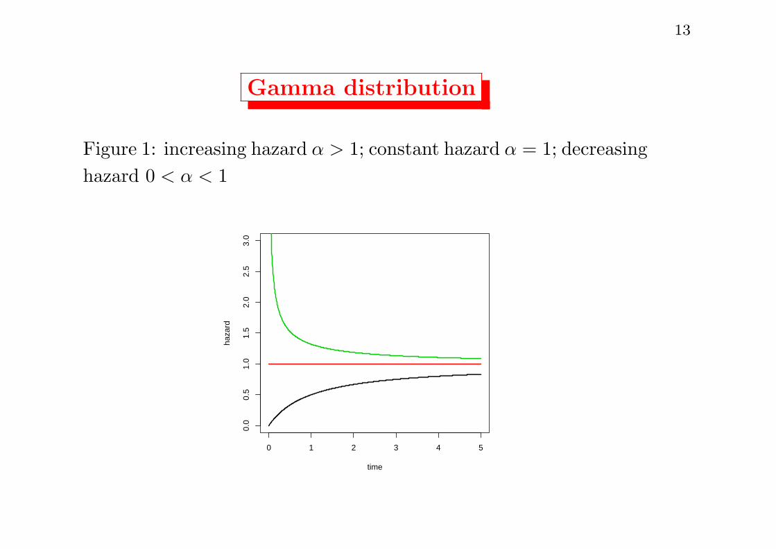
Gamma distribution

• Gamma distribution is a generalization of the simple

exponential distribution.

• Be careful about the parametrization G(α, λ), α, λ > 0 :

1. The density function

f(t) =λαtα−1e−λt

Γ(α)∝ tα−1e−λt,

where

Γ(α) =

∫ ∞

0

tα−1e−tdt

is the Gamma function. For integer α, Γ(α) = (α− 1)!.

2. There is no close formulae for survival or hazard function.

12

Gamma distribution

• E(T ) = αλ−1.

• Var(T ) = αλ−2.

• If Ti ∼ G(αi, λ), i = 1, · · · ,K and Ti, i = 1, · · · ,K are

independent, then

K∑i=1

Ti ∼ G(K∑i=1

αi, λ).

• G(1, λ) ∼ EXP(λ). (A generalization of the exponential

distribution)

13

Gamma distribution

Figure 1: increasing hazard α > 1; constant hazard α = 1; decreasing

hazard 0 < α < 1

0 1 2 3 4 5

0.0

0.5

1.0

1.5

2.0

2.5

3.0

time

haza

rd

14

Weibull distribution

• Weibull distribution is also a generalization of the simple

exponential distribution.

• Be careful about the parametrization W (p, λ), λ > 0(scale

parameter) and p > 0(shape parameter):

1. S(t) = e−(λt)p

2. f(t) = pλ(λt)p−1e−(λt)p ∝ tp−1e−(λt)p .

3. h(t) = pλ(λt)p−1 ∝ tp−1

4. H(t) = (λt)p.

15

Weibull distribution

• E(T ) = λ−1Γ(1 + 1/p).

• Var(T ) = λ−2[Γ(1 + 2/p)− {Γ(1 + 1/p)}2

]• W (1, λ) ∼ EXP(λ).

• W (p, λ) ∼ {EXP(λp)}1/p

16

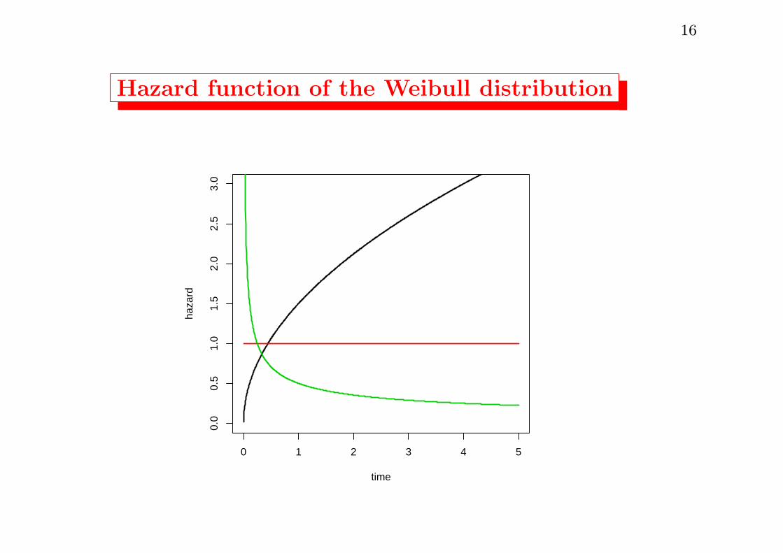
Hazard function of the Weibull distribution

0 1 2 3 4 5

0.0

0.5

1.0

1.5

2.0

2.5

3.0

time

haza

rd

17

Log-normal distribution

• The log-normal distribution is another commonly used

parametric distribution for characterizing the survival time.

• LN(µ, σ2) ∼ exp{N(µ, σ2)}

• E(T ) = eµ+σ2/2

• Var(T ) = e2µ+σ2

(eσ2 − 1)

18

The hazard function of the log-normal distribution

0.0 0.2 0.4 0.6 0.8 1.0

0.0

0.5

1.0

1.5

2.0

2.5

3.0

time

haza

rd

mu=0mu=1mu=−1

19

Generalized gamma distribution

• The generalized gamma distribution becomes popular due to

its flexibility.

• Again be careful about its parametrization GG(α, p, λ) :

• f(t) = pλ(λt)α−1e−(λt)p/Γ(α/p) ∝ tα−1e−(λt)p

• S(t) = 1− γ{α/p, (λt)p}/Γ(α/p), where

γ(s, x) =

∫ x

0

ts−1e−tdt

is the incomplete gamma function.

20

Generalized gamma distribution

• For k = 1, 2, · · ·

E(T k) =Γ {(α+ k)/p}λkΓ(α/p)

• If p = 1, GG(α, 1, λ) ∼ G(α, λ)

• if α = p, GG(p, p, λ) ∼ W (p, λ)

• if α = p = 1, GG(1, 1, λ) ∼ EXP(λ)

• The generalized gamma distribution can be used to test the

adequacy of commonly used Gamma, Weibull and Exponential

distributions, since they are all nested within the generalized

gamma distribution family.

21

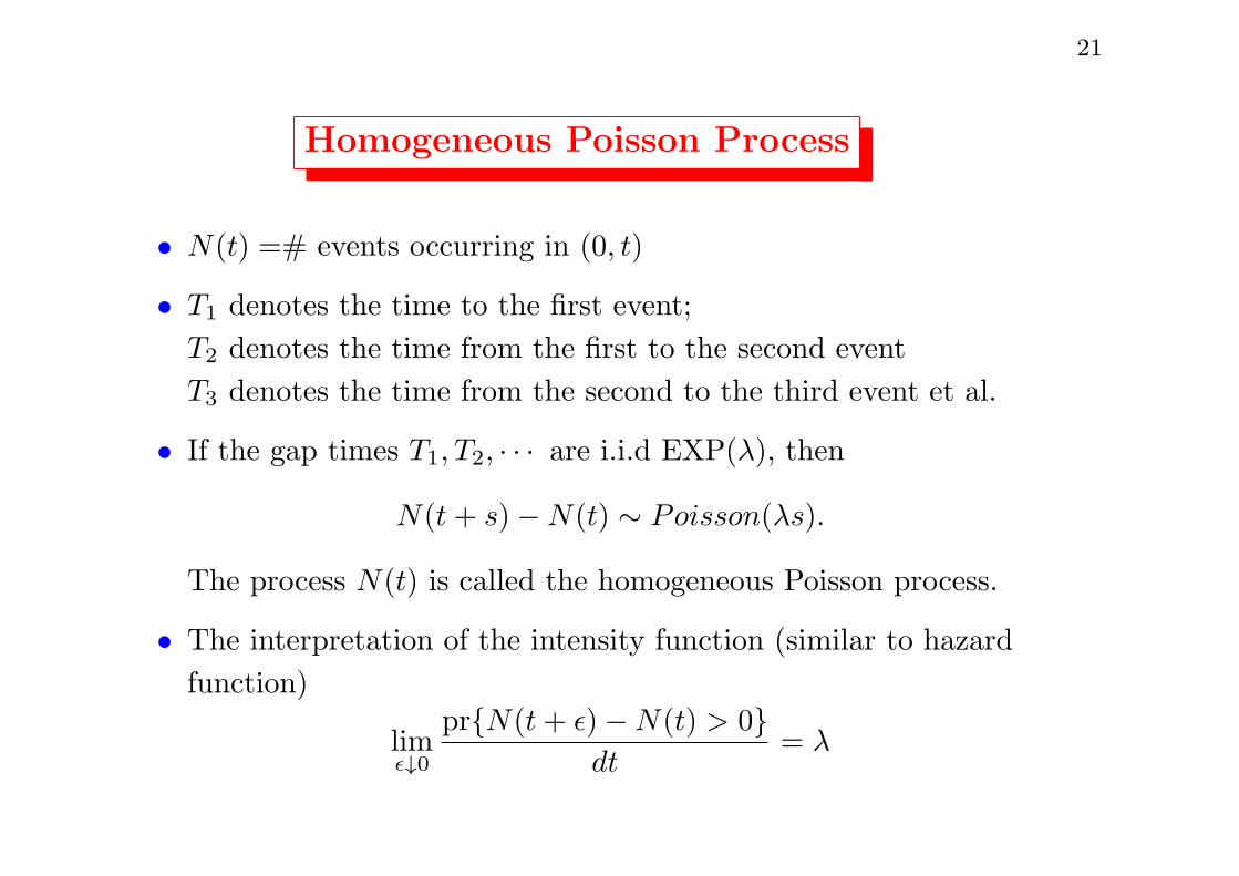
Homogeneous Poisson Process

• N(t) =# events occurring in (0, t)

• T1 denotes the time to the first event;

T2 denotes the time from the first to the second event

T3 denotes the time from the second to the third event et al.

• If the gap times T1, T2, · · · are i.i.d EXP(λ), then

N(t+ s)−N(t) ∼ Poisson(λs).

The process N(t) is called the homogeneous Poisson process.

• The interpretation of the intensity function (similar to hazard

function)

limϵ↓0

pr{N(t+ ϵ)−N(t) > 0}dt

= λ

22

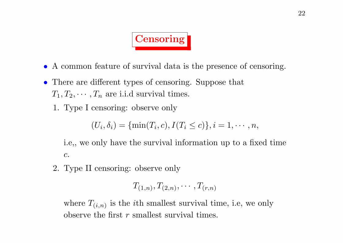
Censoring

• A common feature of survival data is the presence of censoring.

• There are different types of censoring. Suppose that

T1, T2, · · · , Tn are i.i.d survival times.

1. Type I censoring: observe only

(Ui, δi) = {min(Ti, c), I(Ti ≤ c)}, i = 1, · · · , n,

i.e,, we only have the survival information up to a fixed time

c.

2. Type II censoring: observe only

T(1,n), T(2,n), · · · , T(r,n)

where T(i,n) is the ith smallest survival time, i.e, we only

observe the first r smallest survival times.

23

3. Random censoring (The most common type of

censoring): C1, C2, · · · , Cn are potential censoring times

for n subjects, observe only

(Ui, δi) = {min(Ti, Ci), I(Ti ≤ Ci)}, i = 1, · · · , n.

We often treat the censoring time Ci as i.i.d. random

variables in statistical inferences.

4. Interval censoring: observe only (Li, Ui), i = 1, · · · , n such

that Ti ∈ [Li, Ui).

24

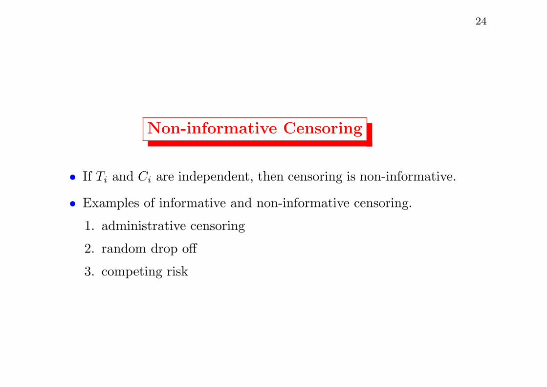
Non-informative Censoring

• If Ti and Ci are independent, then censoring is non-informative.

• Examples of informative and non-informative censoring.

1. administrative censoring

2. random drop off

3. competing risk

25

Non-informative Censoring

• Noninformative censoring condition:

h(t) = limϵ↓0

pr(T ∈ [t, t+ ϵ]|T ≥ t, C ≥ t)

ϵ

• It is slightly weaker than the independence between T and C.

• Consequences of informative censoring:

– There are more than one distribution for (T,C) with

different marginal distribution of T correspond to the same

distribution of (U, δ) = {min(T,C), I(T < C)}.– Based on the distribution (U, δ) alone, it is impossible to

determine the distribution of T.

26

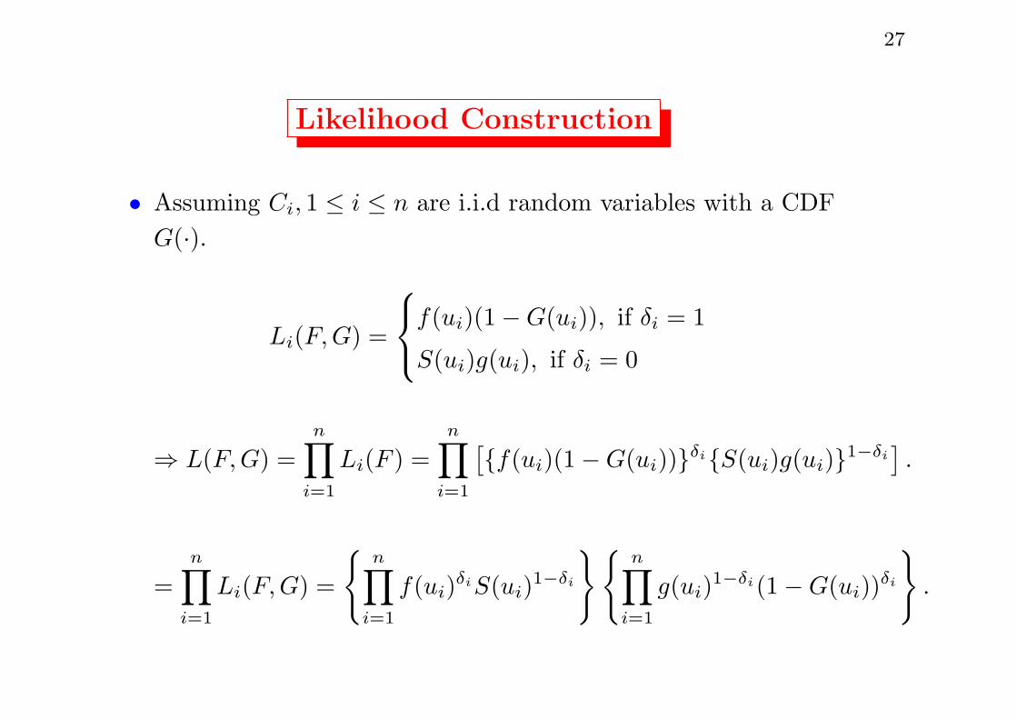
Likelihood Construction

• In the presence of right censoring, we only observe

(Ui, δi), i = 1, · · · , n.

• The likelihood construction must be with respect to the

bivariate random variable (Ui, δi), i = 1, · · · .n.1. If (Ui, δi) = (ui, 1), then Ti = ui, Ci > ui

2. If (Ui, δi) = (ui, 0), then Ti ≥ ui, Ci = ui.

27

Likelihood Construction

• Assuming Ci, 1 ≤ i ≤ n are i.i.d random variables with a CDF

G(·).

Li(F,G) =

f(ui)(1−G(ui)), if δi = 1

S(ui)g(ui), if δi = 0

⇒ L(F,G) =n∏

i=1

Li(F ) =n∏

i=1

[{f(ui)(1−G(ui))}δi{S(ui)g(ui)}1−δi

].

=n∏

i=1

Li(F,G) =

{n∏

i=1

f(ui)δiS(ui)

1−δi

}{n∏

i=1

g(ui)1−δi(1−G(ui))

δi

}.

28

Likelihood Construction

• We have used the noninformative censoring assumption in the

likelihood construction.

• L(F,G) = L(F )× L(G) and therefore the likelihood-based

inference for F can be made based on

L(F ) =n∏

i=1

{f(ui)

δiS(ui)1−δi

}=

n∏i=1

h(ui)δiS(ui)

only.

29

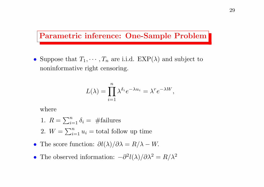
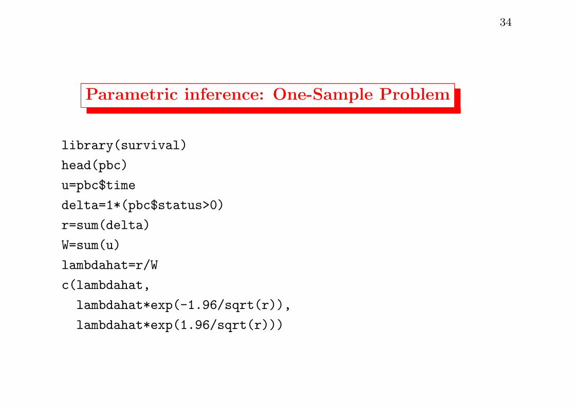
Parametric inference: One-Sample Problem

• Suppose that T1, · · · , Tn are i.i.d. EXP(λ) and subject to

noninformative right censoring.

L(λ) =n∏

i=1

λδie−λui = λre−λW ,

where

1. R =∑n

i=1 δi = #failures

2. W =∑n

i=1 ui = total follow up time

• The score function: ∂l(λ)/∂λ = R/λ−W.

• The observed information: −∂2l(λ)/∂λ2 = R/λ2

30

Parametric inference: One-Sample Problem

• λ = R/W

In epidemiology, the incidence rate is often estimated by the

ratio of total events and total exposure time, which is the MLE

for the constant hazard under the the exponential distribution.

• The information: I(λ) = R/λ2 and

I(λ) = E{I(λ)} = npr(Ci > Ti)/λ2 = np/λ2.

• It follows from the property of MLE

λ− λ√λ2/np

→ N(0, 1)

in distribution as n → ∞.

• λ approximately follows N(λ,R/W 2) for large n.

31

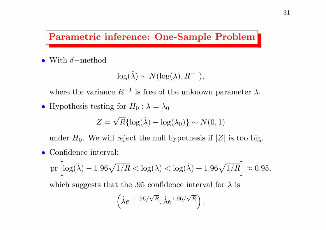
Parametric inference: One-Sample Problem

• With δ−method

log(λ) ∼ N(log(λ), R−1),

where the variance R−1 is free of the unknown parameter λ.

• Hypothesis testing for H0 : λ = λ0

Z =√R{log(λ)− log(λ0)} ∼ N(0, 1)

under H0. We will reject the null hypothesis if |Z| is too big.

• Confidence interval:

pr[log(λ)− 1.96

√1/R < log(λ) < log(λ) + 1.96

√1/R

]≈ 0.95,

which suggests that the .95 confidence interval for λ is(λe−1.96/

√R, λe1.96/

√R).

32

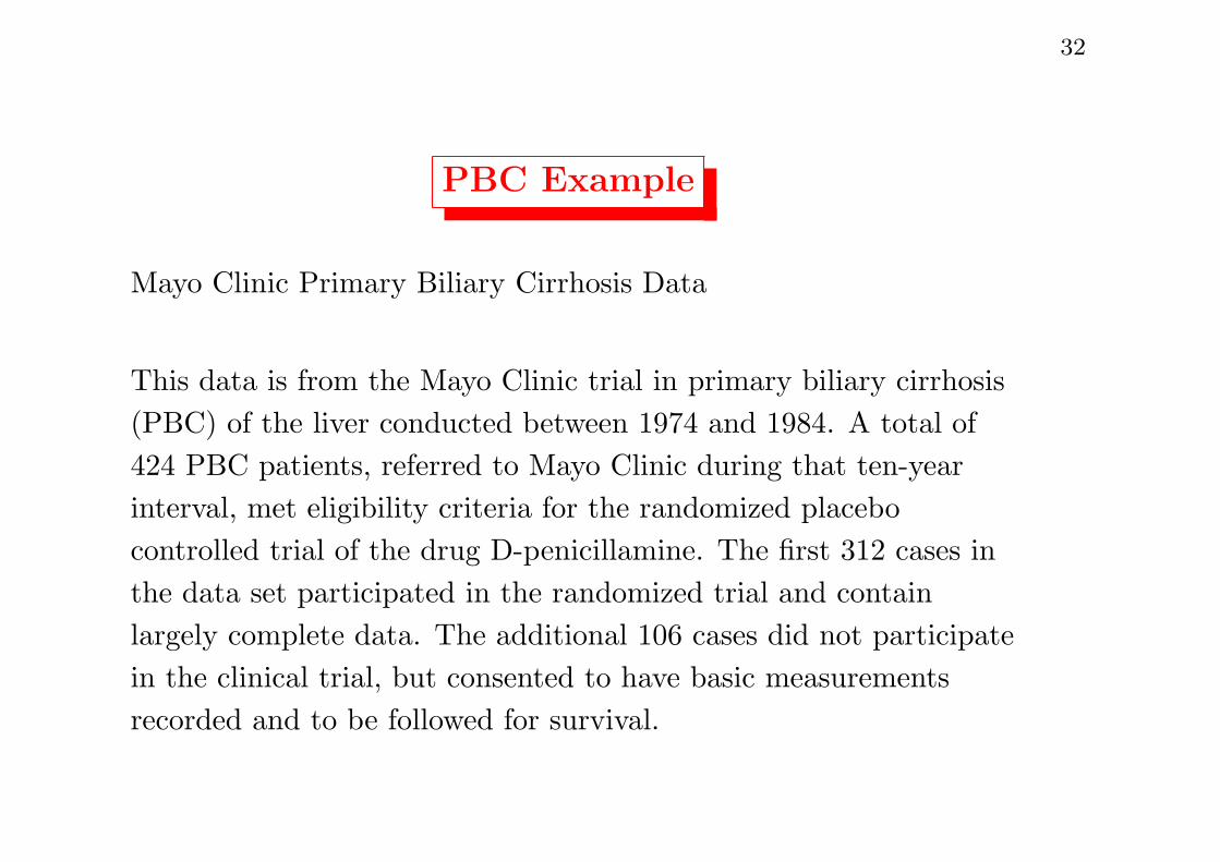
PBC Example

Mayo Clinic Primary Biliary Cirrhosis Data

This data is from the Mayo Clinic trial in primary biliary cirrhosis

(PBC) of the liver conducted between 1974 and 1984. A total of

424 PBC patients, referred to Mayo Clinic during that ten-year

interval, met eligibility criteria for the randomized placebo

controlled trial of the drug D-penicillamine. The first 312 cases in

the data set participated in the randomized trial and contain

largely complete data. The additional 106 cases did not participate

in the clinical trial, but consented to have basic measurements

recorded and to be followed for survival.

33

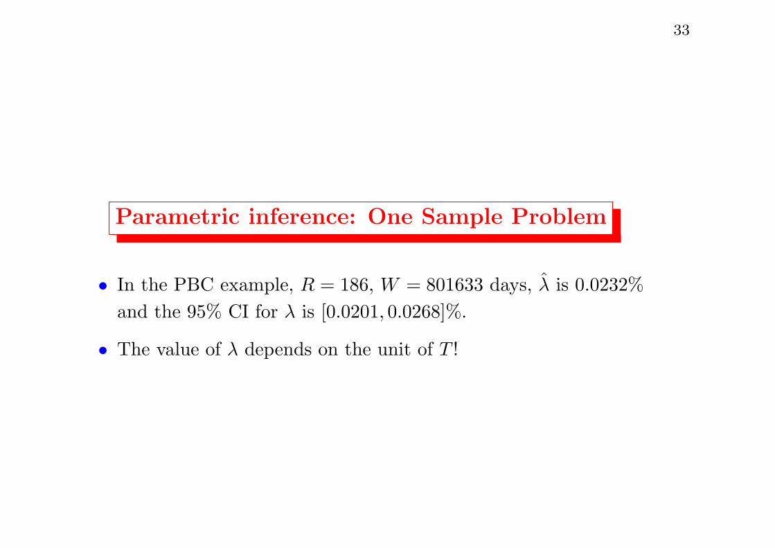
Parametric inference: One Sample Problem

• In the PBC example, R = 186, W = 801633 days, λ is 0.0232%

and the 95% CI for λ is [0.0201, 0.0268]%.

• The value of λ depends on the unit of T !

34

Parametric inference: One-Sample Problem

library(survival)

head(pbc)

u=pbc$time

delta=1*(pbc$status>0)

r=sum(delta)

W=sum(u)

lambdahat=r/W

c(lambdahat,

lambdahat*exp(-1.96/sqrt(r)),

lambdahat*exp(1.96/sqrt(r)))

35

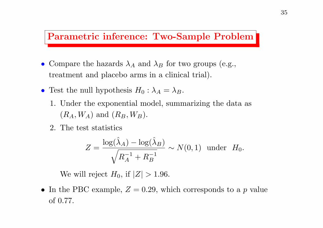
Parametric inference: Two-Sample Problem

• Compare the hazards λA and λB for two groups (e.g.,

treatment and placebo arms in a clinical trial).

• Test the null hypothesis H0 : λA = λB .

1. Under the exponential model, summarizing the data as

(RA,WA) and (RB ,WB).

2. The test statistics

Z =log(λA)− log(λB)√

R−1A +R−1

B

∼ N(0, 1) under H0.

We will reject H0, if |Z| > 1.96.

• In the PBC example, Z = 0.29, which corresponds to a p value

of 0.77.

36

Parametric inference: Two-Sample Problem

library(survival)

head(pbc)

u=pbc$time[1:312]

delta=1*(pbc$status>0)[1:312]

trt=pbc$trt[1:312]

r1=sum(delta[trt==1])

W1=sum(u[trt==1])

lambda1=r1/W1

r2=sum(delta[trt==2])

W2=sum(u[trt==2])

lambda2=r2/W2

z=(log(lambda1)-log(lambda2))/sqrt(1/r1+1/r2)

c(z, 1-pchisq(z^2, 1))

37

Parametric inference: Regression Problem

• z is a p× 1 vector of covariates measured for each subject and

we are interested in assessing the association between z and T

• Observed data: (Ui, δi, zi), i = 1, · · · , n

• Noninformative censoring: Ti ⊥ Ci|Zi = zi (different from

Ti ⊥ Ci)

• What is the appropriate statistical model to link Ti with zi?

38

Parametric inference: Regression Problem

• If we observe (Ti, zi), i = 1, · · ·n, then the linear regression

model can be used:

log(Ti) = β′zi + ϵi,

which is called the accelerated failure time (AFT) model in

survival analysis, where ϵi follows a parametric distribution

such as the extreme value distribution.

• Model the association between the hazard function and

covariates zi

– Ti ∼ EXP(λi)

– log(λi) = log(λ0) + β′zi

• The likelihood function can be used to derive the MLE and

make the corresponding statistical inferences.

39

Parametric Inference

• In practice, the exponential distribution is rarely used due to

its over-simplicity: one parameter λ characterizes the entire

distribution.

• Alternatives such as Weibull, Gamma, Generalized Gamma

distribution and log-normal distribution are more popular, but

they also put specific constraints on the hazard function.

• An intermediate model from parametric to nonparametric

model is the “piecewise exponential” distribution.

40

Parametric Inference

• T1, · · · , Tn i.i.d random variables

• Suppose that the hazard function of T is in the form of

h(t) = λj for vj−1 ≤ t < vj ,

where 0 = v0 < v1 < · · · < vk < vk+1 = ∞ are given cut-off

values.

41

Parametric Inference

Figure 2: The hazard function of piece-wise exponential

h(t)

v v v1 2 k

12 k+1...

...v3 vk-1

k

t

42

Parametric Inference

• L(λ1, · · · , λk+1) = · · ·

• Let Rj and Wj be the total number of events and follow-up

time within the interval [vj , vj+1), respectively. λj = Rj/Wj

• log(λ1), · · · , log(λk+1) are approximately independently

distributed with log(λj) ∼ N(log(λj), R−1j ) for large n.

• The statistical inference for the hazard function follows.