Survival Analysis of Gastric Cancer Patients with ... · Survival Analysis of Gastric Cancer Patients with Incomplete Data ... Survival analysis of gastric cancer patients requires

Original Article

Survival Analysis of Gastric Cancer Patients with Incomplete Data

Abbas Moghimbeigi1,2, Lily Tapak2, Ghodaratolla Roshanaei1,2, and Hossein Mahjub2,3

1Modeling of Noncommunicable Disease Research Center, 2Department of Biostatistics and Epidemiology, 3Research Center for Health Sciences, School of Public Health, Hamadan University of Medical Sciences, Hamadan, Iran

Purpose: Survival analysis of gastric cancer patients requires knowledge about factors that affect survival time. This paper attempted to analyze the survival of patients with incomplete registered data by using imputation methods. Materials and Methods: Three missing data imputation methods, including regression, expectation maximization algorithm, and multiple imputation (MI) using Monte Carlo Markov Chain methods, were applied to the data of cancer patients referred to the cancer institute at Imam Khomeini Hospital in Tehran in 2003 to 2008. The data included demographic variables, survival times, and censored variable of 471 patients with gastric cancer. After using imputation methods to account for missing covariate data, the data were analyzed using a Cox regression model and the results were compared. Results: The mean patient survival time after diagnosis was 49.1±4.4 months. In the complete case analysis, which used information from 100 of the 471 patients, very wide and uninformative confidence intervals were obtained for the chemotherapy and surgery haz-ard ratios (HRs). However, after imputation, the maximum confidence interval widths for the chemotherapy and surgery HRs were 8.470 and 0.806, respectively. The minimum width corresponded with MI. Furthermore, the minimum Bayesian and Akaike information crite-ria values correlated with MI (−821.236 and −827.866, respectively).Conclusions: Missing value imputation increased the estimate precision and accuracy. In addition, MI yielded better results when com-pared with the expectation maximization algorithm and regression simple imputation methods.

Key Words: Survival analysis; Hazard Model; Stomach neoplasms; Regression

J Gastric Cancer 2014;14(4):259-265 http://dx.doi.org/10.5230/jgc.2014.14.4.259

Correspondence to: Abbas Moghimbeigi

Department of Biostatistics and Epidemiology, School of Public Health, Hamadan University of Medical Sciences, Fahmideh Blvd. Mahdieh Ave., Hamadan, IranTel: +98-8118380398, Fax: +98-8118380508E-mail: [email protected] September 7, 2014Revised November 6, 2014Accepted November 6, 2014

Copyrights © 2014 by The Korean Gastric Cancer Association www.jgc-online.org

This is an open-access article distributed under the terms of the Creative Commons Attribution Non-Commercial License (http://creativecommons.org/licenses/by-nc/3.0) which permits unrestricted noncommercial use, distribution, and reproduction in any medium, provided the original work is properly cited.

Introduction

According to statistics published by the World Health Orga-

nization (WHO) in 2010, most deaths occur from noncontiguous

diseases. According to the statistics, more than 36 million deaths

in 2008 were related to noncontiguous diseases, of which 48%,

21%, and 12% were related to heart disease, cancer and respiratory

disease, respectively.1 In Iran, cancer is the third-leading cause of

death after heart disease and accident. According to the most re-

cent statistics from the Iran Cancer Research Center, in Iran gastric

cancer is the most common type of cancer among men and the

third-most common type among women.2,3

The prognosis of gastric cancer is usually poor,4,5 and therefore

this disease has a high mortality rate. Given the low survival rate

of such patients, it is very important to determine the factors that

influence survival in gastric cancer patients. In Iran, various studies

of gastric cancer patients6-10 and factors influencing their survival

have been conducted using Cox regression modeling. Survival data

analysis and modeling in the context of missing covariates present

three major problems: 1) reduced efficacy because of the irregular

information structure and complexity; 2) the lack of ability to use

available software intended to analyze complete data; and 3) biased

Moghimbeigi A, et al.

260

parameter estimation because of differences between observed

and non-observed data.11 Most researchers exclude subjects with at

least 1 missing data point, resulting in a large amount of data and

analytical inefficacy. Ignoring these missing data leads to biased

estimations results, especially when there is a difference between

the survival durations of patients with at least 1 missing data point

and that of patients with complete data.11

Understanding the mechanism of missing data is a substantial

issue when performing an analysis. There are three mechanisms

of missing data, as follows: when the variable with missing data is

independent of the other variables, the missing data are considered

missing completely at random (MCAR); when the variable with

missing data is dependent on the observed data, the missing data

are called missing at random (MAR); and finally, when the variable

is dependent on missing values, the missing data are missing not at

random. In the first two cases, the mechanism of missing data is

ignored11 because the negative effects of missing data on the esti-

mates are unavoidable and the missing data can be imputed. There

are two types of imputation: simple imputation and multiple impu-

tation (MI). In simple imputation, there is only imputed 1 value for

a missing value, whereas in MI more than 1 independent values are

obtained from imputation model to replace each missing value, and

therefore m completed sets of data are obtained.11

The aim of this study was to conduct a comprehensive compar-

ison of the results of registered factors that affect gastric cancers. To

achieve this, we analyzed primary data with missing values using

two simple imputation methods, regression and expectation maxi-

mization (EM) algorithm, and one MI method based on the Monte

Carlo Markov Chain (MCMC).

Materials and Methods

1. Data

In this paper, data related to the survival of 471 gastric cancer

patients who were referred to the cancer institute at Imam Kho-

meini Hospital, Tehran in 2003 to 2008 were investigated. The

study variables included demographic data such as the age at di-

agnosis and sex; degree of tumor differentiation based on WHO

criteria (weak, moderate, or good); tumor site (cardia, body, or an-

trum); tumor size (cm), pathological stage based on the American

Joint Committee on cancer, 6th edition (II, III, or IV); treatment

type, including chemotherapy (adjuvant, neoadjuvant, or pallia-

tive), radiotherapy, or surgery (resection or palliative bypass; yes/

no); and weight loss (yes/no). Patient survival was registered from

the time of diagnosis to death or the end of the study. Subjects who

could not be contacted directly or who did not die before the end

of the study were considered censored observations.10 All tests were

conducted at a significance level of 0.05.

2. Cox proportional hazards model

To identify the factors influencing patient survival, we used a

general form of the Cox proportional hazards model12:

3

are obtained from imputation model to replace each missing value, and therefore m completed

sets of data are obtained (11).

The aim of this study was to conduct a comprehensive comparison of the results of registered

factors that affect gastric cancers. To achieve this, we analyzed primary data with missing

values using two simple imputation methods, regression and expectation maximization (EM)

algorithm, and one MI method based on the Monte Carlo Markov Chain (MCMC).

Materials and Methods

1. Data

In this paper, data related to the survival of 471 gastric cancer patients who were referred to the

cancer institute at Imam Khomeini Hospital, Tehran in 2003 to 2008 were investigated. The

study variables included demographic data such as the age at diagnosis and sex; degree of tumor

differentiation based on WHO criteria (weak, moderate, or good); tumor site (cardia, body, or

antrum); tumor size (cm), pathological stage based on the American Joint Committee on cancer,

6th edition (II, III, or IV); treatment type, including chemotherapy (adjuvant, neoadjuvant, or

palliative), radiotherapy, or surgery (resection or palliative bypass; yes/no); and weight loss

(yes/no). Patient survival was registered from the time of diagnosis to death or the end of the

study. Subjects who could not be contacted directly or who did not die before the end of the

study were considered censored observations (10). All tests were conducted at a significance

level of 0.05.

2. Cox proportional hazards model

To identify the factors influencing patient survival, we used a general form of the Cox

proportional hazards model (12):

1 1( , , , ) ( ) exp( )p

p i iih t X X h t Xβ

== ∑oK .

The proportional hazards hypothesis was evaluated with a goodness of fit test.

.

The proportional hazards hypothesis was evaluated with a

goodness of fit test.

This model was evaluated in complete cases and after complet-

ing a data set consisting of missing data via the three imputation

methods. Although there are many imputation methods, the per-

formance of these methods depends on the percentage of missing

values, missing data pattern, type, and number of variables, and

sample size. In this work, two simple imputation methods, regres-

sion and EM algorithm, and a MI method based on MCMC were

used to impute absent values in a real data set, followed by a com-

parison of the results.

3. Complete case analysis

This method deletes all cases with at least 1 missing variable;

accordingly, the analyses are conducted using cases in which all

variables have been observed and there are no missing values. The

MCAR hypothesis must be stated when using this method to ob-

tain unbiased estimates. The complete case analysis is suitable for

datasets with few missing values and a large sample size.

4. Regression imputation

In this method, missing values based on predictions from the

regression model are imputed.11 The variable with missing values

is considered a response variable and other variables are predicting

variables; therefore, missing values are predicted as new observa-

tions through a fitted model. In this context, two types of logistic

regression (for nominal and ordinal categorical variables) were used

to handle categorical variables and multiple linear regressions were

used for continuous variable imputations.

5. Expectation maximization algorithm

This iterative method is used to find the maximum likelihood

of parameters in problems with missing data along with the simple

Survival Analysis of Gastric Cancer Patients

261

imputation of missing data.13 This algorithm can be summarized

in 4 stages: replacing the missing values with estimated values,

estimation of parameters, re-estimation of the missing values as-

suming that the new parameter is correct, and a new estimation

of parameters. The algorithm is repeated in a loop that continues

to converge. If the matrix of data Y=(Yobs ,Ymis) has a joint density

function P(Y|θ) and log likelihood function l(Y|θ), the EM algo-

rithm can be rewritten as follows:

5

( 1) ( )arg max ( ( | ) | , )t tobsE l Y Y

θθ θ θ+ =

.

6. Multiple imputations using the Monte Carlo Markov Chain method

MI has three steps. First, each missing value is imputed with a set of acceptable values that

reflect uncertainty about the real value to be imputed. These multiple imputed data are

subsequently analyzed using standard methods available for analyzing complete data, and

multiple analyses are combined to yield the final results.

MI can be conducted using various methods, one of which is Gibbs sampling based on the

MCMC methods. In this model, categorical variables are located among the cells of a table at

the level intersections of these variables with multinomial marginal distributions. On each

categorical variable level, continuous variables are considered to have multivariate normal

distributions with means that differ among cells, and the covariance matrix is considered similar

among all cells. In this model, the missing data mechanism is considered to be random and all

hypotheses of this model are based on ignorable missingness.

Assuming the ignorable missingness mechanism, we can obtain m sets of imputed values in the

form of (1) (2) ( ), ,..., mmis mis misY Y Y by using the Bayesian method and considering a prior distribution of

θ. These imputed values are independent observations of the posterior

density ( | ) ( | , ) ( | )mis obs mis obs obsP Y Y P Y Y P Y dθ θ θ= ∫ . To obtain the missing values, data

augmentation was used in two steps; this represents a special case of Gibbs sampling in which

updated values are obtained from conditional distributions in the case of ( )tmisY and ( )tθ in the tth

iteration, as follows:

.

6. Multiple imputations using the Monte Carlo

Markov Chain method

MI has three steps. First, each missing value is imputed with a

set of acceptable values that reflect uncertainty about the real value

to be imputed. These multiple imputed data are subsequently ana-

lyzed using standard methods available for analyzing complete data,

and multiple analyses are combined to yield the final results.

MI can be conducted using various methods, one of which is

Gibbs sampling based on the MCMC methods. In this model, cat-

egorical variables are located among the cells of a table at the level

intersections of these variables with multinomial marginal distribu-

tions. On each categorical variable level, continuous variables are

considered to have multivariate normal distributions with means

that differ among cells, and the covariance matrix is considered

similar among all cells. In this model, the missing data mechanism

is considered to be random and all hypotheses of this model are

based on ignorable missingness.

Assuming the ignorable missingness mechanism, we can obtain

m sets of imputed values in the form

5

( 1) ( )arg max ( ( | ) | , )t tobsE l Y Y

θθ θ θ+ =

.

6. Multiple imputations using the Monte Carlo Markov Chain method

MI has three steps. First, each missing value is imputed with a set of acceptable values that

reflect uncertainty about the real value to be imputed. These multiple imputed data are

subsequently analyzed using standard methods available for analyzing complete data, and

multiple analyses are combined to yield the final results.

MI can be conducted using various methods, one of which is Gibbs sampling based on the

MCMC methods. In this model, categorical variables are located among the cells of a table at

the level intersections of these variables with multinomial marginal distributions. On each

categorical variable level, continuous variables are considered to have multivariate normal

distributions with means that differ among cells, and the covariance matrix is considered similar

among all cells. In this model, the missing data mechanism is considered to be random and all

hypotheses of this model are based on ignorable missingness.

Assuming the ignorable missingness mechanism, we can obtain m sets of imputed values in the

form of (1) (2) ( ), ,..., mmis mis misY Y Y by using the Bayesian method and considering a prior distribution of

θ. These imputed values are independent observations of the posterior

density ( | ) ( | , ) ( | )mis obs mis obs obsP Y Y P Y Y P Y dθ θ θ= ∫ . To obtain the missing values, data

augmentation was used in two steps; this represents a special case of Gibbs sampling in which

updated values are obtained from conditional distributions in the case of ( )tmisY and ( )tθ in the tth

iteration, as follows:

of by us-

ing the Bayesian method and considering a prior distribution of θ.

These imputed values are independent observations of the posterior

density P(Ymis|Yobs)=∫P(Ymis|Yobs ,θ)P(θ|Yobs)dθ. To obtain the missing

values, data augmentation was used in two steps; this represents a

special case of Gibbs sampling in which updated values are ob-

tained from conditional distributions in the case of

5

( 1) ( )arg max ( ( | ) | , )t tobsE l Y Y

θθ θ θ+ =

.

6. Multiple imputations using the Monte Carlo Markov Chain method

MI has three steps. First, each missing value is imputed with a set of acceptable values that

reflect uncertainty about the real value to be imputed. These multiple imputed data are

subsequently analyzed using standard methods available for analyzing complete data, and

multiple analyses are combined to yield the final results.

MI can be conducted using various methods, one of which is Gibbs sampling based on the

MCMC methods. In this model, categorical variables are located among the cells of a table at

the level intersections of these variables with multinomial marginal distributions. On each

categorical variable level, continuous variables are considered to have multivariate normal

distributions with means that differ among cells, and the covariance matrix is considered similar

among all cells. In this model, the missing data mechanism is considered to be random and all

hypotheses of this model are based on ignorable missingness.

Assuming the ignorable missingness mechanism, we can obtain m sets of imputed values in the

form of (1) (2) ( ), ,..., mmis mis misY Y Y by using the Bayesian method and considering a prior distribution of

θ. These imputed values are independent observations of the posterior

density ( | ) ( | , ) ( | )mis obs mis obs obsP Y Y P Y Y P Y dθ θ θ= ∫ . To obtain the missing values, data

augmentation was used in two steps; this represents a special case of Gibbs sampling in which

updated values are obtained from conditional distributions in the case of ( )tmisY and ( )tθ in the tth

iteration, as follows:

and θ(t) in

the tth iteration, as follows:

Under reasonable conditions such as t→∞, the values of (θ(t),

5

( 1) ( )arg max ( ( | ) | , )t tobsE l Y Y

θθ θ θ+ =

.

6. Multiple imputations using the Monte Carlo Markov Chain method

MI has three steps. First, each missing value is imputed with a set of acceptable values that

reflect uncertainty about the real value to be imputed. These multiple imputed data are

subsequently analyzed using standard methods available for analyzing complete data, and

multiple analyses are combined to yield the final results.

MI can be conducted using various methods, one of which is Gibbs sampling based on the

MCMC methods. In this model, categorical variables are located among the cells of a table at

the level intersections of these variables with multinomial marginal distributions. On each

categorical variable level, continuous variables are considered to have multivariate normal

distributions with means that differ among cells, and the covariance matrix is considered similar

among all cells. In this model, the missing data mechanism is considered to be random and all

hypotheses of this model are based on ignorable missingness.

Assuming the ignorable missingness mechanism, we can obtain m sets of imputed values in the

form of (1) (2) ( ), ,..., mmis mis misY Y Y by using the Bayesian method and considering a prior distribution of

θ. These imputed values are independent observations of the posterior

density ( | ) ( | , ) ( | )mis obs mis obs obsP Y Y P Y Y P Y dθ θ θ= ∫ . To obtain the missing values, data

augmentation was used in two steps; this represents a special case of Gibbs sampling in which

updated values are obtained from conditional distributions in the case of ( )tmisY and ( )tθ in the tth

iteration, as follows:

) become stationary and the missing values are obtained from

this distribution after convergence. The EM algorithm is used to

generate the initial data augmentation values. In the MI method, 5

data sets were generated, and each of the 5 imputed sets were ana-

lyzed using the Cox regression model; we then combined the rules

to obtain the final results. In this method, each data set is analyzed

separately, and the results are combined according to specific rules

to yield a general result comprising uncertainty about the missing

data.14

7. Statistical software

Cox proportional hazard model fitting and regression imputa-

tion were performed using SPSS ver. 16.0 (SPSS Inc., Chicago, IL,

USA). A MIX package of R software (version 2.15.1; Institute for

Statistics and Mathematics, Vienna University of Economics and

Business, Vienna, Austria; available at http://www.r-project.org/

index.html) was used for MI and EM algorithm imputation (imp.

mix and da.mix functions).

Results

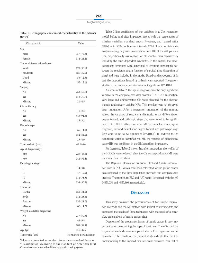
Overall, 153 patients (32.5%) died; the remaining patients were

censored at the end of the study or dropped out. The mean patient

survival time after diagnosis was 49.1±4.4 months, with a maxi-

mum survival time of 125 months. Table 1 lists the demographic

and clinical characteristics of the patients as percentages along with

data missingness information. As shown in Table 1, the following

variables have missing values: tumor differentiation degree (12.1%),

tumor site (14.2%), tumor size (54.8%), pathological stage (50.5%),

chemotherapy (3.2%), radiotherapy (4.9%), surgery (4.5%), and

weight loss (39.9%). The overall missing data rate was 79%, requir-

ing the removal of 371 of the 471 patients.

Regarding the missing data problem, the missing data propor-

tion is not the only criterion for imputation. The missing data

mechanisms and patterns have greater impacts on research results

than does the missing data proportion.15 In order to obtain reliable

results from the imputation, acceptance of the MAR or MCAR

hypothesis is a key assumption. In the present study, Little’s MCAR

test16 was performed using SPSS ver. 16.0 and the MCAR as-

sumption was not rejected (P=0.658). In addition, we considered

the missing and non-missing data as two separate groups for all

variables. We then compared the gender and age of the groups us-

ing the chi-square test and t-test. All P-values exceeded 0.05 and

confirmed the assumption of MCAR for these data.

Moghimbeigi A, et al.

262

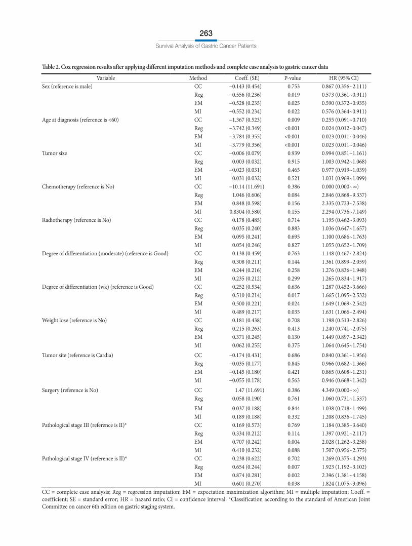
Table 2 lists coefficients of the variables in a Cox regression

model before and after imputation along with the percentages of

missing variables, standard errors, P-values, and hazard ratios

(HRs) with 95% confidence intervals (CIs). The complete case

analysis setting only used information from 100 of the 471 patients.

The proportionality assumption for all variables was evaluated by

including the time-dependent covariates. In this regard, the time-

dependent covariates were generated by creating interactions be-

tween the predictors and a function of survival time (logarithm of

time) and were included in the model. Based on the goodness of fit

test, the proportional hazard hypothesis was supported. The gener-

ated time-dependent covariates were not significant (P＞0.05).

As seen in Table 2, the age at diagnosis was the only significant

variable in the complete case data analysis (P＜0.001). In addition,

very large and uninformative CIs were obtained for the chemo-

therapy and surgery variable HRs. This problem was not observed

after imputation. After a regression imputation of the missing

values, the variables of sex, age at diagnosis, tumor differentiation

degree (weak), and pathologic stage (IV) were found to be signifi-

cant (P＜0.001). Furthermore, after MI the variables of sex, age at

diagnosis, tumor differentiation degree (weak), and pathologic stage

(IV) were found to be significant (P＜0.001). In addition to the

significant variables identified via MI, the variable of pathological

stage (III) was significant in the EM algorithm imputation.

Furthermore, Table 2 shows that after imputation, the widths of

the HR CIs were reduced; also, the CIs corresponding to MI were

narrower than the others.

The Bayesian information crirerion (BIC) and Akaike informa-

tion criteria (AIC) values have been calculated for the gastric cancer

data subjected to the three imputation methods and complete case

analysis. The minimum BIC and AIC values correlated with the MI

(-821.236 and -827.866, respectively).

Discussion

This study evaluated the performances of two simple imputa-

tion methods and the MI method with respect to missing data and

compared the results of these techniques with the result of a com-

plete case analysis of gastric cancer data.

Diagnosis of the prognostic factors of gastric cancer is very im-

portant when determining the type of treatment. The effects of the

imputation methods were compared after a Cox regression model

evaluation. The results of the present study indicate that the CIs

corresponding to the imputed data sets were narrower than that of

Table 1. Demographic and clinical characteristics of the patients (n=471)

Characteristic Value

Sex

Male 357 (75.8)

Female 114 (24.2)

Tumor differentiation degree

Weak 170 (36.1)

Moderate 186 (39.5)

Good 58 (12.3)

Missing 57 (12.1)

Surgery

No 262 (55.6)

Yes 188 (39.9)

Missing 21 (4.5)

Chemotherapy

No 11 (2.3)

Yes 445 (94.5)

Missing 15 (3.2)

Radiotherapy

No 66 (14.0)

Yes 382 (81.1)

Missing 23 (4.9)

Time to death (mo) 49.1±4.4

Age at diagnosis (yr)

<60 229 (48.6)

>60 242 (51.4)

Pathological stage*

II 14 (3.0)

III 47 (10.0)

IV 172 (36.5)

Missing 238 (50.5)

Tumor site

Cardia 160 (34.0)

Body 112 (23.8)

Antrum 132 (28.0)

Missing 67 (14.2)

Weight loss (after diagnosis)

No 237 (50.3)

Yes 46 (9.8)

Missing 188 (39.9)

Age (yr) 59.0±12.7

Tumor size (cm) 5.53±2.6 (54.8% missing)

Values are presented as number (%) or mean±standard deviation. *Classification according to the standard of American Joint Committee on cancer 6th edition on gastric staging system.

Survival Analysis of Gastric Cancer Patients

263

Table 2. Cox regression results after applying different imputation methods and complete case analysis to gastric cancer data

Variable Method Coeff. (SE) P-value HR (95% CI)Sex (reference is male) CC −0.143 (0.454) 0.753 0.867 (0.356~2.111)

Reg −0.556 (0.236) 0.019 0.573 (0.361~0.911)EM −0.528 (0.235) 0.025 0.590 (0.372~0.935)MI −0.552 (0.234) 0.022 0.576 (0.364~0.911)

Age at diagnosis (reference is <60) CC −1.367 (0.523) 0.009 0.255 (0.091~0.710)Reg −3.742 (0.349) <0.001 0.024 (0.012~0.047)EM −3.784 (0.355) <0.001 0.023 (0.011~0.046)MI −3.779 (0.356) <0.001 0.023 (0.011~0.046)

Tumor size CC −0.006 (0.079) 0.939 0.994 (0.851~1.161)Reg 0.003 (0.032) 0.915 1.003 (0.942~1.068)EM −0.023 (0.031) 0.465 0.977 (0.919~1.039)MI 0.031 (0.032) 0.521 1.031 (0.969~1.099)

Chemotherapy (reference is No) CC −10.14 (11.691) 0.386 0.000 (0.000~∞)Reg 1.046 (0.606) 0.084 2.846 (0.868~9.337)EM 0.848 (0.598) 0.156 2.335 (0.723~7.538)MI 0.8304 (0.580) 0.155 2.294 (0.736~7.149)

Radiotherapy (reference is No) CC 0.178 (0.485) 0.714 1.195 (0.462~3.093)Reg 0.035 (0.240) 0.883 1.036 (0.647~1.657)EM 0.095 (0.241) 0.695 1.100 (0.686~1.763)MI 0.054 (0.246) 0.827 1.055 (0.652~1.709)

Degree of differentiation (moderate) (reference is Good) CC 0.138 (0.459) 0.763 1.148 (0.467~2.824)Reg 0.308 (0.211) 0.144 1.361 (0.899~2.059)EM 0.244 (0.216) 0.258 1.276 (0.836~1.948)MI 0.235 (0.212) 0.299 1.265 (0.834~1.917)

Degree of differentiation (wk) (reference is Good) CC 0.252 (0.534) 0.636 1.287 (0.452~3.666)Reg 0.510 (0.214) 0.017 1.665 (1.095~2.532)EM 0.500 (0.221) 0.024 1.649 (1.069~2.542)MI 0.489 (0.217) 0.035 1.631 (1.066~2.494)

Weight lose (reference is No) CC 0.181 (0.438) 0.708 1.198 (0.513~2.826)Reg 0.215 (0.263) 0.413 1.240 (0.741~2.075)EM 0.371 (0.245) 0.130 1.449 (0.897~2.342)MI 0.062 (0.255) 0.375 1.064 (0.645~1.754)

Tumor site (reference is Cardia) CC −0.174 (0.431) 0.686 0.840 (0.361~1.956)Reg −0.035 (0.177) 0.845 0.966 (0.682~1.366)EM −0.145 (0.180) 0.421 0.865 (0.608~1.231)MI −0.055 (0.178) 0.563 0.946 (0.668~1.342)

Surgery (reference is No) CC 1.47 (11.691) 0.386 4.349 (0.000~∞)Reg 0.058 (0.190) 0.761 1.060 (0.731~1.537)

EM 0.037 (0.188) 0.844 1.038 (0.718~1.499)MI 0.189 (0.188) 0.332 1.208 (0.836~1.745)

Pathological stage III (reference is II)* CC 0.169 (0.573) 0.769 1.184 (0.385~3.640)Reg 0.334 (0.212) 0.114 1.397 (0.921~2.117)EM 0.707 (0.242) 0.004 2.028 (1.262~3.258)MI 0.410 (0.232) 0.088 1.507 (0.956~2.375)

Pathological stage IV (reference is II)* CC 0.238 (0.622) 0.702 1.269 (0.375~4.293)Reg 0.654 (0.244) 0.007 1.923 (1.192~3.102)EM 0.874 (0.281) 0.002 2.396 (1.381~4.158)MI 0.601 (0.270) 0.038 1.824 (1.075~3.096)

CC = complete case analysis; Reg = regression imputation; EM = expectation maximization algorithm; MI = multiple imputation; Coeff. = coefficient; SE = standard error; HR = hazard ratio; CI = confidence interval. *Classification according to the standard of American Joint Committee on cancer 6th edition on gastric staging system.

Moghimbeigi A, et al.

264

the complete analysis, indicating improved estimate precision. Gen-

erally, a wider interval implies a less efficient approach. MI is the

best approach in terms of efficiency because it yielded the narrow-

est CI. Furthermore, the complete case analysis yielded the worst

results based on this criterion. Additionally, the MI performance

was superior according to the BIC and AIC criteria for comparing

models. The key point in the present study analysis is that imputa-

tion techniques improved the identification of factors that influence

survival. We found that the variables of sex, age at diagnosis, tumor

differentiation degree (weak), and pathologic stage (IV) all had sig-

nificant effects on survival in gastric cancer patients.

In the MI setting, missing data were imputed five times to

provide highly accurate estimates and avoid random effects on im-

putation. Two other imputation techniques (EM algorithm and re-

gression) are also suitable when working with missing data. How-

ever, these techniques only replace each missing value with a single

value. Accordingly, imputation uncertainty and estimate precision

are not taken into account and may be diminished because of the

high proportion of missing data.17 In this regard, single imputation

cannot represent any additional uncertainty that might arise when

the reason for data missingness is unknown.

In addition, even if the proportion of missing data for each vari-

able is low, this may cause serious problems in multivariate model-

ing when patients with missing data are scattered throughout the

dataset.17 This is because the number of complete cases available for

analysis might be substantially reduced, thus increasing the risk of

bias consequent to case exclusion. Power reduction is another con-

sequence of complete case analysis, and case deletion may result in

biased regression coefficients if the remaining cases are not repre-

sentative of the entire sample.18

Several studies have confirmed the satisfactory performance of

the MI technique in a simulation based on various criteria for han-

dling missing covariates. Peng and Zhu,19 in a study to evaluate the

performance of MI, concluded that MI had a lower bias and better

efficiency and coverage with respect to estimating true parameter

values than did the EM algorithm and complete case analysis.

In their study, Baneshi and Talei17 showed that the exclusion

of cases with missing data led to bias and imprecise estimates and

suggested that missing data imputation should be a primary step

before conducting any modeling. Molenberghs et al.,20 in a study to

compare different imputation techniques, concluded with a strong

recommendation for MI. In addition, Marshall et al.21,22 concluded

that MI might be the preferred approach for handling data miss-

ingness. Accordingly, the results of the present study confirm those

previous findings.

Generally, invalid results are the usual consequence of exclud-

ing cases with missing data and analyzing only those subjects with

complete data (complete case analysis).

Instead, before conducting any analysis, a close examination

should be conducted in an attempt to understand the reasons for

data missingness. Once the MCAR or MAR mechanism is as-

sumed, missing data imputation should be performed before any

modeling practice.

However, these results are only based on a single realistic popu-

lation and the MCAR mechanism. Therefore, a limitation of this

study is that the obtained results are not fully generalizable to other

populations with differing distributions, correlations, and missing

data mechanisms; hence, further studies are required.

This study addressed the performance of three imputation

techniques with respect to a realistic data set from gastric cancer

patients. Based on two evaluation criteria, the performance of MI

was superior to that of simple imputation techniques of EM algo-

rithm and regression. Furthermore, these three imputation methods

yielded better performances than the complete case analysis. How-

ever, further studies are required because these results were based

only on a single data set.

Acknowledgments

This article comprises part of an MSc thesis in Biostatistics and

was supported by Hamadan University of Medical Sciences.

References

1. World Health Organization (WHO). Death and DALY esti-mates by cause [Internet]. Geneva: WHO; [cited 2014 Sep 6]. Available from: http://www.who.int/entity/healthinfo/statistics/bodgbddeathdalyestimates.xls.

2. Mohagheghi M, ed. Annual Report of Tehran Cancer Registry 1999. Tehran: The Cancer Institute Publication, 2004.

3. Mohagheghi M, Musavi Jarahi A, Shariat Torbaghan S, Zeraati H, eds. Annual Report of Tehran University of Medical Scienc-es District Cancer Registry 1997. Tehran: The Cancer Institute Publication, 1998.

4. Biglarian A, Hajizadeh E, Gouhari MR, Khodabakhshi R. Survival analysis of patients with gastric adenocarcinomas and factors related. Kowsar Med J 2008;12:337-347.

5. Zeraati H, Mahmoudi M, Kazemnejad A, Mohammad K. Post-

Survival Analysis of Gastric Cancer Patients

265

operative survival in gastric cancer patients and its associated factors: a time dependent covariates model. Iranian J Public Health 2006;35:40-46.

6. Barnard J, Meng XL. Applications of multiple imputation in medical studies: from AIDS to NHANES. Stat Method Med Res 1999;8:17-36.

7. Burton A, Altman DG. Missing covariate data within cancer prognostic studies: a review of current reporting and proposed guidelines. Br J Cancer 2004;91:4-8.

8. Pourhoseingholi MA, Hajizadeh E, Moghimi Dehkordi B, Safaee A, Abadi A, Zali MR. Comparing Cox regression and parametric models for survival of patients with gastric carci-noma. Asian Pac J Cancer Prev 2007;8:412-416.

9. Roushanaei G, Kazemnejad A, Sedighi S. Postoperative sur-vival estimation of gastric cancer patients in cancer institute of Tehran, Imam Khomeini hospital and its relative factors. Sci J Hamadan Univ Med Sci 2010;17:13-18.

10. Im WJ, Kim MG, Ha TK, Kwon SJ. Tumor size as a prognostic factor in gastric cancer patient. J Gastric Cancer 2012;12:164-172.

11. Little RJ, Rubin DB, eds. Statistical Analysis with Missing Data. New York: John Wiley & Sons, 2002.

12. Kleinbaum DG, Klein M, eds. Survival Analysis. 3rd ed. New York: Springer, 2012.

13. Barzi F, Woodward M. Imputations of missing values in prac-tice: results from imputations of serum cholesterol in 28 cohort studies. Am J Epidemiol 2004;160:34-45.

14. Javaras KN, Van Dyk DA. Multiple imputation for incom-plete data with semicontinuous variables. J Am Stat Assoc 2003;98:703-715.

15. Tabachnick BG, Fidell LS, eds. Using Multivariate Statistics. 6th ed. Needham Heights (MA): Allyn & Bacon, 2012.

16. Little RJ. A test of missing completely at random for multivari-ate data with missing values. J Am Stat Assoc 1988;83:1198-1202.

17. Baneshi MR, Talei A. Impact of imputation of missing data on estimation of survival rates: an example in breast cancer. Ira-nian J Cancer Prev 2012;3:127-131.

18. Altman DG, Bland JM. Missing data. BMJ 2007;334:424.19. Peng CYJ, Zhu J. Comparison of two approaches for handling

missing covariates in logistic regression. Educ Psychol Meas 2008;68:58-77.

20. Molenberghs G, Williams PL, Lipsitz SR. Prediction of survival and opportunistic infections in HIV-infected patients: a com-parison of imputation methods of incomplete CD4 counts. Stat Med 2002;21:1387-1408.

21. Marshall A, Altman DG, Holder RL. Comparison of imputa-tion methods for handling missing covariate data when fitting a Cox proportional hazards model: a resampling study. BMC Med Res Methodol 2010;10:112.

22. Marshall A, Altman DG, Royston P, Holder RL. Comparison of techniques for handling missing covariate data within prog-nostic modelling studies: a simulation study. BMC Med Res Methodol 2010;10:7.