TRIBHUVAN UNIVERSITY Kathmandu Engineering College Kalimati, Kathmandu Report No. 2062/BCE/Survey (EG625) A Report on Survey Camp 2064 at NEATC, Kharipati (For the partial fulfillment of the requirement for the Bachelor’s Degree in Civil Engineering) Submitted By: Submitted to: Group: J The Department of Civil Engineering Rabindra Subedi - 62109/BCE/062 Kathmandu Engineering Subash Thapa Magar - 62115/BCE/062 Kalimati, Kathmandu Nawin Kumar Acharya - 62106/BCE/062 Sukriti Suvedi - 62118/BCE/062 Bhuban Singh - 62084/BCE/062 29 th Jestha 2065

Welcome message from author
This document is posted to help you gain knowledge. Please leave a comment to let me know what you think about it! Share it to your friends and learn new things together.
Transcript

TRIBHUVAN UNIVERSITY
Kathmandu Engineering College Kalimati, Kathmandu
Report No. 2062/BCE/Survey (EG625)
A Report on Survey Camp 2064 at NEATC, Kharipati
(For the partial fulfillment of the requirement for the Bachelor’s Degree in Civil Engineering)
Submitted By: Submitted to: Group: J The Department of Civil Engineering Rabindra Subedi - 62109/BCE/062 Kathmandu Engineering Subash Thapa Magar - 62115/BCE/062 Kalimati, Kathmandu Nawin Kumar Acharya - 62106/BCE/062 Sukriti Suvedi - 62118/BCE/062 Bhuban Singh - 62084/BCE/062
29th Jestha 2065

ABSTRACT
The main objective of the Survey Camp organized by the civil department is to provide an opportunity to consolidate and update the practical & theoretical knowledge in engineering surveying in the actual field condition and habituate to work in different environment with different people. In this survey camp we are supposed to survey a given plot in all its aspect and work on road and bridge alignment and prepare a topographic maps, maps of road and bridge alignment with proper cross section and profile and its topography fulfilling all technical requirements.
This survey camp helped us to build our confidence to conduct engineering survey on required accuracy and we assume that it would be of great use in our future engineering works.
Group J
PREFACE This survey report is truly based on our knowledge gained from the two weeks field trip organized for the partial fulfillment of the requirement for the Bachelor’s Degree in Civil Engineering encoded as EG625CE as per our syllabus in third year first part. This surveying has been able to impart us the great opportunity to consolidate and review the practical and theoretical knowledge on surveying, which we gained in second year.
We have been able to achieve the true objectives of survey and upgrade the knowledge as handling of the instrument, working procedure, problem solving and field booking precisely. This survey camp gave us the practical knowledge of overcoming the technical difficulties and developing a skill in tackling it. It encouraged us to cope with the team members, as the surveying involved all the members equally during the field procedures, calculations and plotting and report preparations.
Actually this survey camp promoted us in developing the ideas of the major and minor traversing, RL transformation, detailing, detailing by plane tabling, topographical map preparation, road and bridge site surveying, curve setting, orientation etc.
In this way the survey camp was really fruitful and it enhanced to enrich our confidence to carryout engineering survey on required accuracy in near future.
ACKNOWLEDGEMENT
This report is the outcome of our work done in two weeks survey camp in NEATC, Kharipati, and Bhaktapur. This camp was organized by Kathmandu Engineering College, Department of Civil Engineering, for the students of 2062 Batch.
We worked on the various aspects of surveying such as topographical and road surveying in NEATC, Kharipati Area and bridge Site at Punyamata River Panauti, Kavre. Our group consisted of five members whose names are listed on the cover page. We worked together as a group in the survey camp – 2064.
We express our great thanks to our respected teachers Er.Narayan Pd. Subedi, Er.Pawan Gautam, Er. Arjun Pd. Parajuli, Er. Ramesh Subedi, Er.Rajendra Soti, Er. Rangan Bhattrai who were very supportive and played a key role in successively finishing the survey camp. We are also thankful to the Department of Civil Engineering, which gave us such a golden opportunity to gain the knowledge on different aspects of surveying that will definitely prove beneficial in every step of the civil engineering projects in near future. We would like to convey our sincere thanks to the management of our college for choosing such a healthy and creative environment for teaching and learning practice for such a long period of fifteen days.
We also would like to thank to the survey camp staffs Mr. Dipendra Shrestha, Mr. Deepak Upreti, Mr. Santosh and Mr. Ram Krishna for their great help during the camp.
Our heartily thanks goes to all other seniors and individuals who helped and guided us with the experiences they had, for the preparation of the Survey Report.
We are also grateful to the very friendly Kharipati natives and the staffs of the NEATC who indirectly helped us for the completion of the project.
Last but not the least we must thank Ar. Chand S. Rana, the principal of KEC for encouraging us during our camping and also the KEC teachers’ team for participating in the DOHORI and Pop Song singing program and on the last evening of our camp for happy ending of our tiresome but very memorable camping.
And at last we would like to thank the readers for their concern in our report. This report is the outcome of our huge and continuous efforts for about 4 months including the survey period.
Group - J

TABLE OF CONTENT ABSTRACT PREFACE ACKNOWLEDGEMENT LIST OF TABLES ……………………………………………………………………………… 1
I. INTRODUCTION……………………………………………………………………… 2 1.1. Background…………………………………………………………………....... 2 1.2. Objectives………………………………………………………………………. 3 1.3. Project Area……………………………………………………………………. 4 1.4. Norms………………………………………………………………………….. 5 1.5. Working Schedule……………………………………………………………… 7
II. TRAVERSING………………………………………………………………………… 9
2.1. Introduction ………………………………………………………………. …… 9 2.2. Principle of theodolite survey ……………………………………………… 9 2.3. Methods of theodolite traversing…………………………………………… 9 2.4. Latitude, Departure and closing error……………………………………… 10 2.5. Balancing of consecutive co-ordinates ……………………………………. 11 2.6. Objective ………………………………………………………………..….. … 11 2.7. Major Traverse ………………………………………………………………… 11
2.7.1. Introduction ……………………………………………………………… 11 2.7.2. Methodology …………………………………………………………… 11
2.7.2.1. Reconnaissance……………………………………………….. 11 2.7.2.2. Pegging………………………………………………………….12 2.7.2.3. Linear measurement…………………………………………… 12 2.7.2.4. Angular measurement………………………………………… 12 2.7.2.5. Correction of internal angles……………………………………12 2.7.3.6. Bearing Computation of Traverse legs………………………… 12 2.7.3.7. Coordinate Computation of Traverse Stations………………… 13 2.7.3.8. Plotting of Major Traverse Stations…………………………… 14 2.7.3.9. Sample Calculation…………………………………………… 14 2.7.3.10. Final Co-ordinate sheet……………………………………… 14
2.8. MINOR TRAVERSE………………………………………………………… 14
2.8.1. Introduction…………………………………………………………. 14 2.8.2. Methodology………………………………………………………… 14 2.8.2.1. Reconnaissance………………………………………………… 14 2.8.2.2. Marking and fixing control points…………………………… 14 2.8.2.3. Measurement of Traverse Legs………………………………… 14 2.8.2.4. Measurement of Interior Angles……………………………… 14 2.8.2.5. Bearing Computation of the Traverse Legs…………………… 15 2.8.2.6. Coordinates Computation of Minor control points……………… 15 2.8.2.7. Plotting of Minor Traverse Stations…………………………… 15 2.8.3. Instruments used………………………………………………… 15 2.8.4. Final Co-ordinate Sheet………………………………………… 15 2.8.5. Other Observation and calculation Sheet……………………… 16
III. LEVELLING ………………………………………………………………………… 16
3.1. Introduction……………………………………………………………………16 3.2. Objective………………………………………………………………………16 3.3. Fly Leveling…………………………………………………………………...16
3.3.1. Introduction……………………………………………………………...16 3.3.2. Procedure…………………………………………………………………17 3.3.3. Observation and Calculation………………………………………….......17 3.3.4. Conclusion……………………………………………………………… 17
3.4. Two Peg Test…………………………………………………………………17 3.4.1. Introduction………………………………………………………………17 3.4.2. Observation……………………………………………………………… 17 3.4.3. Level Transfer from B.M. to T.B.M………………………………………18
3.4.3.1. Observation and calculation……………………………………19 3.4.4. Level transfer from T.B.M. to Major Traverse ………………………… 19
3.4.4.1. Observation and Calculation………………………………… 19 3.4.5. Level transfer from Major to Minor Traverse……………………………..19
3.4.5.1. Observation and calculation……………………………………19 3.5. Reciprocal Leveling……………………………………………………………19
IV. TACHEOMETRIC DETAILING…………………………………………………….20 4.1. Introduction……………………………………………………………………20 4.2. Objective……………………………………………………………………….20 4.3. General theory & Methodology…………………………………………… 21
4.3.1. Measurement and Data……………………………………………………21 4.3.2. Field procedure ………………………………………………………… 21 4.3.3. Calculation ………………………………………………………………. 21 4.3.4. Accuracy and Precision……………………………………………………21 4.3.5. Instrument…………………………………………………………………22
4.4. Contouring……………………………………………………………………..22 4.4.1. Methods of Locating Contour…………………………………………….22 4.4.2. Interpolation of Contours…………………………………………………23
4.5. Conclusion…………………………………………………………………… 24 4.6. Observation and calculation…………………………………………………. 24
V. ORIENTATION……………………………………………………………………. 25 5.1. To determine the position of unknown point by the method of Intersection…25
5.1.1. Introduction………………………………………………………………25 5.1.2. Objective……………………………………………………………… 25 5.1.3. Instruments Required…………………………………………………… 25 5.1.4. Observation and Calculation…………………………………………… 26 5.1.5. Result…………………………………………………………………… 30
5.2. To determine the unknown position of Instrument ………………………….31 5.2.1. Instruments Required……………………………………………………31 5.2.2. Objectives……………………………………………………………….31 5.2.3. Theory…………………………………………………………………...34 5.2.4. Observations And Calculations…………………………………………32 5.2.5. Result…………………………………………………………………... 38
VI. CURVES…………………………………………………………………………… 39 6.1. Introduction………………………………………………………………... 39 6.2. Simple Circular Curves…………………………………………………… 39 6.3. Transition Curves………………………………………………………… 40
6.4. Vertical Curves………………………………………………………… 44 6.5. Field Procedure………………………………………………………….40 6.6. Observation And Calculation……………………………………………46
VII. ROAD SURVEY………………………………………………………………..49 7.1. Introduction…………………………………………………………….. 49 7.2. Objectives ……………………………………………………………….49 7.3. Norms (Technical Specification)………………………………………. 49 7.4. Equipments…………………………………………………………….. 50 7.5. Methodology……………………………………………………………50
7.5.1. Reconnaissance…………………………………………………….50 7.5.2. Horizontal Alignment ……………………………………………..50 7.5.3. Curve fitting with inaccessible ……………………………………51 7.5.4. Levelling …………………………………………………………. 51 7.5.5. Longitudinal Section……………………………………………… 51 7.5.6. Cross section ……………………………………………………… 51 7.5.7. Calculations and plotting …………………………………………..52 7.5.8. Observation and Calculation……………………………………… 52 7.5.9. Comments And Conclusion……………………………………… 53
VIII. BRIDGE SITE SURVEY…………………………………………………… 54 8.1. Introduction ……………………………………………………………54 8.2. Objectives………………………………………………………………54 8.3. Brief Description of the Area………………………………………… 54 8.4. Hydrology, Geology & Soil………………………………………… 54 8.5. Technical Specification……………………………………………… 55 8.6. Instrument required ………………………………………………… 55 8.7. Methodology………………………………………………………… 55
8.7.1. Reconnaissance………………………………………………… 55 8.7.2. Fixing the stations……………………………………………… 56 8.7.3. Topographic Survey…………………………………………… 56 8.7.4. Longitudinal Section…………………………………………… 56 8.7.5. Cross –Section……………………………………………………57 8.7.6. Detailing………………………………………………………… 57 8.7.7. Reciprocal Leveling…………………………………………… 57
8.7.7.1. Observation and Calculation………………………… 58 8.8. Observations and Calculations……………………………………… 59 8.9. Computation And Plotting………………………………………… 59 8.10. Comments And Conclusion………………………………………… 59
IX. CONCLUSION AND RECOMMENDATIONS…………………………… 61 9.1. Conclusion…………………………………………………………… 61 9.2. Recommendations…………………………………………………… 61
X. BIBLIOGRAPHY………………………………………………………… 62 XI. ANNEX…………………………………………………………………… 63
Appendix A Data and Calculation Appendix A1: Topographic Survey Appendix A2: Bridge Site Survey Appendix A3: Road Site Survey

Appendix B Map and Drawing Appendix B1: Major Traverse Appendix B2: Tachometric Detailing of Minor Traverse Appendix B3: Bridge Site (Triangulation and Tachometric) Appendix B4: Road Site Graph No. 1(A) – Bridge (Longitudinal Section) Graph No. 1(B) - Bridge (Cross Section) Graph No. 2(A) - Road (Longitudinal Section) Graph No. 2(B) - Road (Cross Section)

1
Survey Camp 2064 Group J
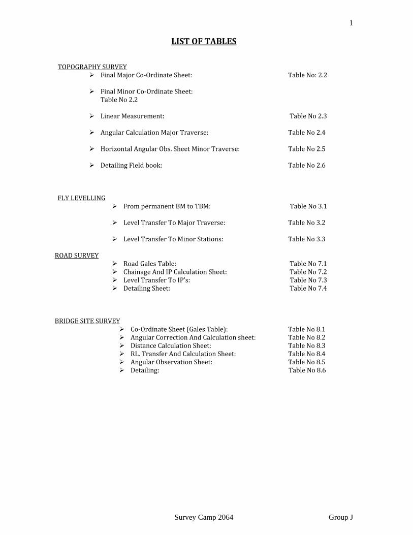
LIST OF TABLES TOPOGRAPHY SURVEY
Final Major Co‐Ordinate Sheet: Table No: 2.2
Final Minor Co‐Ordinate Sheet: Table No 2.2
Linear Measurement: Table No 2.3
Angular Calculation Major Traverse: Table No 2.4
Horizontal Angular Obs. Sheet Minor Traverse: Table No 2.5
Detailing Field book: Table No 2.6
FLY LEVELLING From permanent BM to TBM: Table No 3.1
Level Transfer To Major Traverse: Table No 3.2
Level Transfer To Minor Stations: Table No 3.3
ROAD SURVEY
Road Gales Table: Table No 7.1 Chainage And IP Calculation Sheet: Table No 7.2 Level Transfer To IP’s: Table No 7.3 Detailing Sheet: Table No 7.4
BRIDGE SITE SURVEY Co‐Ordinate Sheet (Gales Table): Table No 8.1 Angular Correction And Calculation sheet: Table No 8.2 Distance Calculation Sheet: Table No 8.3 RL. Transfer And Calculation Sheet: Table No 8.4 Angular Observation Sheet: Table No 8.5 Detailing: Table No 8.6

2
Survey Camp 2064 Group J
I. INTRODUCTION
1.1. BACKGROUND:
Surveying in the simplest form is the measure of relative position of points or absolute measurement of any feature on or beneath the earth surface by using distance, angle, and elevation measuring instruments. Land‐ area surveys are made to determine the relative horizontal and vertical position of topographic features and to establish reference marks to guide construction or to indicate land boundaries. Reconnaissance of the area is followed by a preliminary survey; a map and then a plan are prepared based on the plan. Survey is used to establish property boundaries involving a through knowledge of real‐estate laws as well as skills in survey techniques.
Topographic maps are graphical representations of natural and man‐made features of parts of the Earth’s surface plotted to scale. They provide the bases for specialized maps and data for compilation of generalized maps of smaller scale. It is impossible to start railways, roads, canals, tunnels, transmission power line, dams, and bridge site location, even building without preliminary survey. Before starting any structure or launching the ambitious projects on the earth surface or below the ground, the role of survey is critical. Survey never means measuring and drawing the ground feature to the corresponding scale and portraying, these vertical relationships with others nearly. It encloses the wide area and the system of surveying and the application is increasing day by day. Besides using Theodolite traversing on the land, now remote sensing system and photogrammetric has changed the survey procedure in new format. In true sense the modern scientific methodology is approaching to the true value, which is never defined in terms of survey, with very high precision. Although modern sophisticated instruments such as EDM has introduced new establishment but the basic principle is remains unchanged. However it is true that we are more nearer to their true value with this modern equipment and handling is very easy. For the purpose of water line, sanitary or road also the relative altitude are required, which is ascertain by the levelling. Even the details of the enclosed area and the ground nature can be portrayed in combined form as topographic map. The whole land can be surveyed in different plots and can be united into a single map. The main thing is not to violate the basic survey principles viz. working from whole to part, consistency of work, accuracy required according to scale and independent check.
Above mention things are perquisite while handling the project and for gaining experience such type of survey has to be done and what we do in the survey can is not different from it. In other words it is the combat in field with the theory of survey as tools.
The main objective of the surveying course allocated for Civil Engineering
Students is to promote them the basic knowledge of different surveying techniques relevant to
Civil Engineering works in their professional practice. The surveying is one of the most
important subject matter before and during the civil engineering works like construction of
Highway, Irrigation project, Construction of building etc.
Survey Instruction Committee, Kathmandu Engineering College, organized the
Survey Camp 2064 at Kharipati. The duration of Survey Camp was 15 days, from 2064
Kartik 7 to Kartik 21 NEATC premises at Kharipati V.D.C., Bhaktapur, Nepal.
1.2. Objectives:
The main objective of the camp is to provide a basic knowledge of practical implementation
of different survey works, which is to be encountered in future. It enhances the practical

3
Survey Camp 2064 Group J
knowledge thereby implementing different works and in other side it involves the self‐
confidence eternally. The main objectives of the survey camp can be enlisted as follows:
• To become familiar with the surveying problems that may arise during the field works
in future.
• To became familiar with the instruments, their functions and handling the surveying
instruments for its use in surveying works.
• To become familiar with the spirit and importance of teamwork, as surveying is not a
single person's work.
• To complete the given projects in scheduled time and thus know the value of time.
• To collect required data in the field in systematic ways.
• To compute and manipulate the observed data in the required accuracy and present it in
diagrammatic and tabular form in order to understand by other Engineers and related
personnel easily.
• To tackle the mistakes and incomplete data from the field while in office work.
• To give the good opportunity to use the theoretical background on engineering survey in
the practical life.
• To know the complete methods of report preparation.
Our project was mainly divided into three parts. They were:
I. Topographical Survey of a part of NEATC premises.
II. Bridge Site Survey in Punyamata Khola, Panauti.
III. Road Alignment Survey at NEATC Premises.
a. Topographical Survey:
The first major work during the survey camp was the preparation of
topographical map of NEATC, Kharipati. The topographical map is defined as the map
representing the positions of all the features in x and y‐axis along with the vertical positions
with the help of contour lines. In order to prepare the map, the survey was done in the given
area using the major and minor traverses. Also the elevations (R.L.) were transferred from
the given Benchmark (B.M.) firstly to all the traverse stations and then to all the detailed
points. The contour lines were drawn later by performing the necessary calculations. Finally
the detailed Topographic Map including the major and minor traverse, details and contour
lines of the surveyed area was plotted in the given scale. All the calculations in tabular form
along with the topographical map are presented here with this report.
b. Bridge Site Survey:
4
Survey Camp 2064 Group J
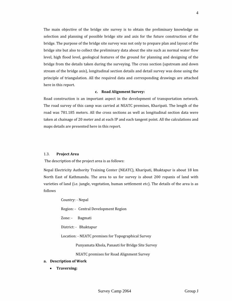
The main objective of the bridge site survey is to obtain the preliminary knowledge on
selection and planning of possible bridge site and axis for the future construction of the
bridge. The purpose of the bridge site survey was not only to prepare plan and layout of the
bridge site but also to collect the preliminary data about the site such as normal water flow
level, high flood level, geological features of the ground for planning and designing of the
bridge from the details taken during the surveying. The cross section (upstream and down
stream of the bridge axis), longitudinal section details and detail survey was done using the
principle of triangulation. All the required data and corresponding drawings are attached
here in this report.
c. Road Alignment Survey:
Road construction is an important aspect in the development of transportation network.
The road survey of this camp was carried at NEATC premises, Kharipati. The length of the
road was 781.185 meters. All the cross sections as well as longitudinal section data were
taken at chainage of 20 meter and at each IP and each tangent point. All the calculations and
maps details are presented here in this report.
1.3. Project Area
The description of the project area is as follows:
Nepal Electricity Authority Training Center (NEATC), Kharipati, Bhaktapur is about 18 km
North East of Kathmandu. The area to us for survey is about 200 ropanis of land with
varieties of land (i.e. jungle, vegetation, human settlement etc). The details of the area is as
follows
Country: ‐ Nepal
Region: ‐ Central Development Region
Zone: ‐ Bagmati
District: ‐ Bhaktapur
Location: ‐ NEATC premises for Topographical Survey
Punyamata Khola, Panauti for Bridge Site Survey
NEATC premises for Road Alignment Survey
a. Description of Work
• Traversing:
5
Survey Camp 2064 Group J
i) No. of Major Traverse Stations =19
ii) No. of Minor Traverse Stations=6
iii) No. of Link Traverse Stations =6
• Road Alignment:
ii) Length of the road: 781.185m
iii) Cross section: 10m left and 10m right on both sides from central line.
• Bridge Site Survey:
i) Bridge span: 54.915m
iii) Cross section up to 120m on upstream and 60m on downstream at 20m interval.
1.4. Norms (Technical Specifications):
All the students at the camp had to work under some norms provided by survey instruction
committee. The norms are listed as follows:
The given work had to be completed within 15 days keeping 2 days each for road
site and bridge site.
The proper handling and care of the instrument was the responsibility of the entire
group.
The major and minor traverse had to be fixed in such a way that these points were to
be followed:
a) At least two consecutive stations should be visible from a station.
b) Two‐way measurement for one traverse leg should be done. The discrepancy should
be greater than 1:2000
c) The number of traverse stations should be minimum.
d) Two sets of horizontal angle should be taken in major traverse & only one set in
minor traverse. The difference between the mean angles of two set reading should
be within the least count of the theodolite.
e) The leg ratio of the traverse stations should not be less than 1:2 for major traverse
and not less than 1:3 for minor traverse, where ratio stands for the longest side:
shortest side
f) All the available checks should be applied to the traverse and adjusted using
appropriate method.
g) After the completion of the fieldwork, the plotting of the traverse along with details
and the contour lines has to be done thus preparing the topographical map of the
worked area.
h) Plotting should be done by independent co‐ordinate.

6
Survey Camp 2064 Group J
i) Fly leveling should be done to transfer RL from the BM. The permissible error in the
leveling should not be greater than ±25√k mm, where k is the distance in km. All
three‐hair readings should be taken in this case.
j) Fly leveling should determine the RL of all the major and minor traverse station. In
this case, only central hair reading should be taken.
k) The permissible closing error for closed loop should within ±C√ minute, where N =
no of stations and usually C is taken as 1.
i. AREA ACTIVITIES:
• TOPOGRAPHICAL MAP PREPARATION
Scale: 1:500
Area: 1.5 to 2 Hectares
Paper size for plotting : A1 or A2
Contour interval: 1m (depending upon the site relief)
Major Traverse scale 1:1000 (or adjustable)
ii. CONTROL POINT ESTABLISHMENT:
At least 12 stations (Main control stations)
Two set of horizontal angle
One set of vertical angle
Two‐way length measurement (taping), check or compare with the
Tachometric distance.
Traverse line orientation, check by graphically (Telescopic Alidade).
Vertical control by Levelling, check by trigonometrical levelling.
Fly levelling carry out at least 1 kilometer away.
Special Technique of Surveying:
Tacheometric detailing by Resection and Intersection (Three
points at least in each case)
Plane table for detailing (using Telescopic alidade) as
required.
iii. LINEAR STRUCTURE ACTIVITIES (Road alignment survey)
• At least 500 m stretch
• Scale Plan 1:1000
• L –section scale: Vertical 1:100, Horizontal 1:1000 (H:V =1:100
• Left/right observation: 10 m minimum on either side
iv. Curve Setting :
• Horizontal curve:
Simple Circular: by both linear and angular method

7
Survey Camp 2064 Group J
Transition: by both linear and angular
• Lead survey by Abney level.
v. BRIDGE SITE SURVEY:
• Up stream: 60m (at least)
• Down stream : 120m (at least)
• Scale for plotting minimum area of observation or coverage.
• Plan 1:500
• Contour interval: 2 m or depending upon site topography.
• Cross‐section: every 20m interval: Scale: Same for both vertical and horizontal (H=V=1:100)
• Observation should be taken 20m beyond the bank on either side of the river or at least 10m above the HFL (high flood level) cover line (contour line).
vi. Instruments Used:
The instruments required during the survey camp are as follows:
Level Machine
Staffs
Theodolite
Magnetic Compass
Measuring tape (30m, 50m)
Ranging rods
Hammer
Arrow
Pegs
Plane table with telescopic alidade
1.5. WORKING SCHEDULE:
Working Schedules no.
Day Survey field Work
1 7th kartik Reconnaissance
2 8th kartik Major Traverse Survey
3 9th Kartik Major and Minor Traverse Survey
4 10th Kartik Two peg Test and Fly Levelling
5 11th Kartik Major, Minor Traverse & Computation
6 12th Kartik Road Site Survey
7 13th Kartik Road Site Survey
8 14th Kartik Coordinate Computation; Adjustment
& plotting

8
Survey Camp 2064 Group J
Project Title: Survey Camp 2064
Location: NEATC, Kharipati, Bhaktapur, Nepal
Duration: Kartik 7th to Kartik 21th
Working time: 07:00a.m. To 6:00 p.m.
Class: 7:00‐8:00 p.m. (daily)
Methodology:
The methodology of the surveying is based on the principle of surveying, which includes:
• Working from Whole to the Parts
• Independent Check
• Accuracy Required
• Consistency in Work
9 15th Kartik Tacheometry/ Detailing
10 16th Kartik Tacheometry/ Detailing
11 17th Kartik Intersection; Resection; Curve Ranging &
Plane table /Theodolite Detailing
12 18th Kartik Bridge Site Survey
13 19th Kartik Bridge Site Survey
14 20th Kartik Tacheometry/ Detailing
15 21th kartik Detail completion; inspection &Checking
9
Survey Camp 2064 Group J
II. TRAVERSING
2.1. INTRODUCTION:
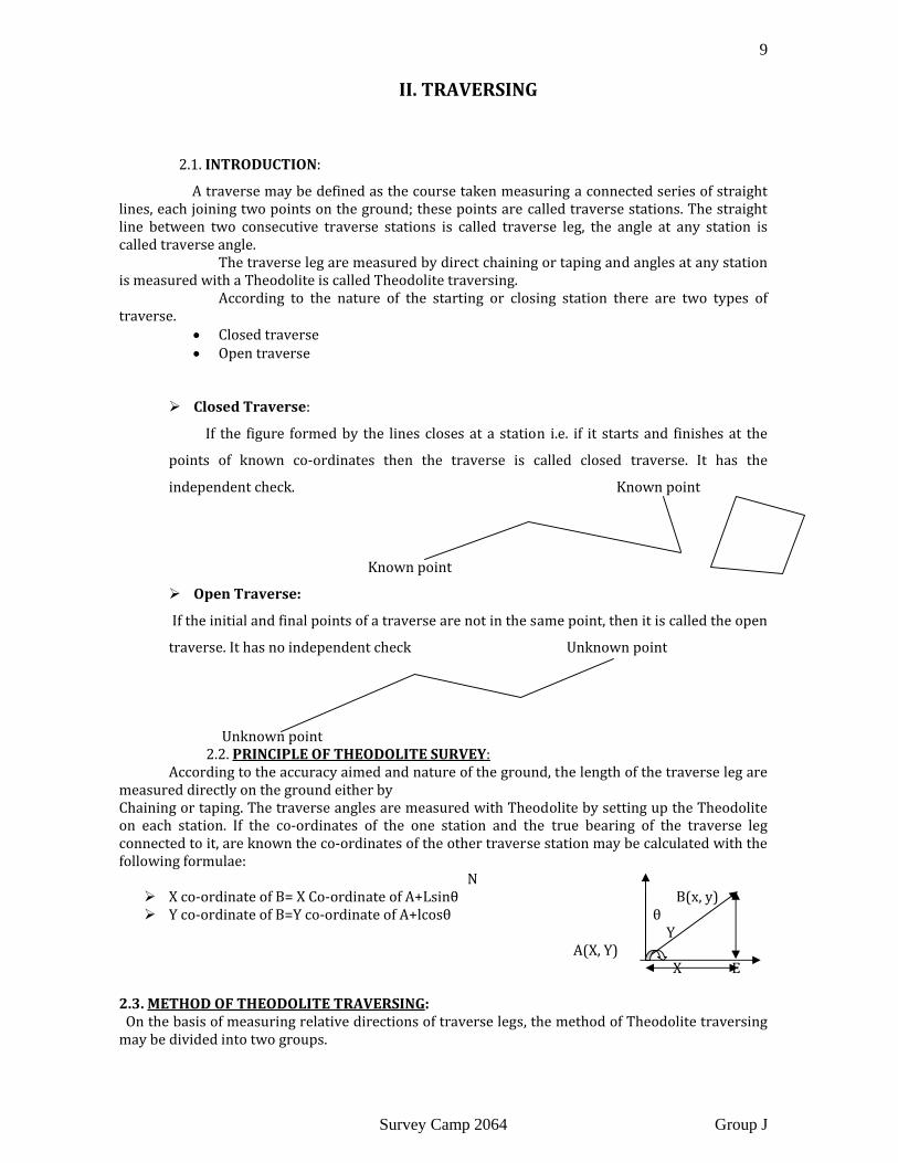
A traverse may be defined as the course taken measuring a connected series of straight lines, each joining two points on the ground; these points are called traverse stations. The straight line between two consecutive traverse stations is called traverse leg, the angle at any station is called traverse angle. The traverse leg are measured by direct chaining or taping and angles at any station is measured with a Theodolite is called Theodolite traversing. According to the nature of the starting or closing station there are two types of traverse.
• Closed traverse • Open traverse
Closed Traverse:
If the figure formed by the lines closes at a station i.e. if it starts and finishes at the
points of known co‐ordinates then the traverse is called closed traverse. It has the
independent check. Known point
Known point
Open Traverse:
If the initial and final points of a traverse are not in the same point, then it is called the open
traverse. It has no independent check Unknown point
Unknown point 2.2. PRINCIPLE OF THEODOLITE SURVEY:
According to the accuracy aimed and nature of the ground, the length of the traverse leg are measured directly on the ground either by Chaining or taping. The traverse angles are measured with Theodolite by setting up the Theodolite on each station. If the co‐ordinates of the one station and the true bearing of the traverse leg connected to it, are known the co‐ordinates of the other traverse station may be calculated with the following formulae: N
X co‐ordinate of B= X Co‐ordinate of A+Lsinθ B(x, y) Y co‐ordinate of B=Y co‐ordinate of A+lcosθ θ Y
A(X, Y) X E
2.3. METHOD OF THEODOLITE TRAVERSING: On the basis of measuring relative directions of traverse legs, the method of Theodolite traversing may be divided into two groups.

10
Survey Camp 2064 Group J
a) By measuring the direct angle between two consecutive traverse leg. b) By measuring the direct bearing of the traverse leg.
THEODOLITE TRAVERSING BY ANGLE MEASUREMENT: This method is generally adopted for long traverse when higher degree of accuracy is required. In this method, bearing of the starting and closing traverse legs are generally determined by making astronomical observations to pole, sun or star. In this method, angle between relative directions of traverse legs, are directly measured with Theodolite. Direct angles measured at different traverse stations may be either included angles or deflected angles. Theodolite traversing by observing included angles: The included angles are those angles which measured on the left side of the direction of traverse. It is customary to run a closed traverse in an anticlockwise direction in which only interior angles are measured. In closed circuits, the accuracy of the angular measurement is easily checked by summing up all the included angles as their total sum should be equal to (2n±4)*90°, where n is no. of traverse legs, the +ve sign is used for exterior angles and negative sign is used for interior angles. Arrows shows the direction of traverse. N F E
A s D B C Fig: ‐ A closed traverse with interior angles. B C 2.4. LATITUDE AND DEPARTURE:‐ The latitude or Northing (N) of a survey line is defined as the co‐ordinate measured parallel to the assumed meridian. The Departure or Easting of a survey line is defined as the co‐ordinate measured at right angle to the assumed meridian. The negative latitude is Southing and Positive Latitude is Northing. Similarly the–ve, Departure is Westing and positive departure is Easting. To calculate the Latitude (L) and Departure (D), the following relation is applied. Latitude (L) =l*Cosθ Departure (D) =l*sinθ Where l & θ are length and reduced bearing of traverse leg. CALCULATION OF CLOSING ERROR: In a complete circuit, the sum of the north Latitudes must be equal to the sum of the south latitudes; the sum of easting must be equal to the sum of westing. If linear as well as angular measurement of the traverse along with their computations is correct. If not the distance between the starting station and position obtained by the calculation is called closing error. The closing error can be expressed as a fraction which is: Closing Error/Perimeter of traverse Where, Closing error= ∆E2 ∆N2

11
Survey Camp 2064 Group J
2.5. BALANCING THE CONSECUTIVE COORDINATES: Generally, there are two methods of balancing the consecutive co‐ordinates.
a) BOWDITCH’S METHOD: ‐ This method is employed when linear and angular measurements of the traverse are of equal accuracy.
If, l=length of leg ∑l=perimeter of legs ∑L=Total error in Latitude ∑D=Total error in Departure ∂L=Correction to the Latitude of the leg ∂D=Correction to the Departure of the leg. Then, ∂L= l/∑l *∑L ∂D = l/∑L *∑D b) Transit Rule: ‐ If angular accuracy is more than linear accuracy, then transit rule is
applied. According to this rule, Correction to the latitude of leg=Total error in latitude/Sum of Latitude*Latitude of that leg Correction to the departure of leg = Total error in departure/sum of departure*Departure of that leg The traversing consists the measurement of following
a. Angles between successive lines or bearings of each line
b. The length of each line
2.6. OBJECTIVES:
As the principle of surveying is to work from the whole to the part, precision control
points are fixed by triangulation at distances 5 to 10 Km apart. The theodolite traverse is,
therefore, carried out for the following purposes:
To provide control points for chain surveying, plane tabling and photogrammetric
surveys in flat country.
To fix the alignment of roads, canals, rivers, boundaries, etc. when better accuracy
is required as compared to plane tabling.
To ascertain the co‐ordinates of boundary pillars in numerical terms that can be
preserved for future reference such as forest boundary pillars, international
boundary pillars, etc. In case the pillars get disturbed, their positions can be
relayed with the help of their co‐ordinates.
2.7. MAJOR TRAVERSE:
2.7.1. Introduction: The whole site is enclosed by the framework interconnecting the successive control stations &is known as major traverse. Different works are conducted sequentially and is the brief.
2.7.2. METHODOLOGY:
2.7.2.1. Reconnaissance:
The first step of any survey is reconnaissance. The area given to us at the camp for
detailing was the part of total area of NEATC, Kharipati. As in the case of major traversing,

12
Survey Camp 2064 Group J
reconnaissance was done before fixing minor stations. These minor stations were purposed
in such a way that it covers each and every important detail. Generally eye estimation is
used and rough calculation is done for fixing the traverse legs. Rough reference sketch
principal features such as buildings, roads are prepared. Various difficulties that had arisen
must be preplanned on the mind.
2.7.2.2. Pegging:
After the completion of the reconnaissance the next step to be taken is to fix the major
traverse first and then the minor ones if necessary. Before fixing a traverse station the care
should be taken that the two other stations are visible from this station and the leg ratio
should be maintained as per the specification. After taking the decision of fixing the station
at any point, that point should be marked with the paint or the peg and then finally the
referencing of the stations should be done.
2.7.2.3. Linear Measurement:
Legs were measured with a standard tape in both forward and backward direction. Ranging
was done for the longer tape lengths with eye estimation and stepping method for slopping
ground. Possible errors due to sagging tension force, temperature change were eliminated
by taking convenient distance and following the error prone methods. Linear accuracy was
within 1:2000
2.7.2.4. Angular measurement:
Two‐set readings were taken in each station one with 00 set and next with 900 set. The
difference in face‐left & face‐right reading and interior angle obtained from both set were
different by more than the least‐count of theodolite used on the field. It was checked in the
field while observation was taken. If it is not the case the reading should be repeated until
the desired accuracy is gained
2.7.2.5. Correction of internal angles:
The traverse must be closed and it was checked by the formula = (2n – 4) x 90°
Where, n = no of traverse stations.
The sum of the interior angles was not equal to (2n – 4) x 90° and the error was equally
distributed in each internal angle of traverse stations.
Adopted accuracy = ± C N minutes Where, C =1 and N= no. of total traverse stations
13
Survey Camp 2064 Group J
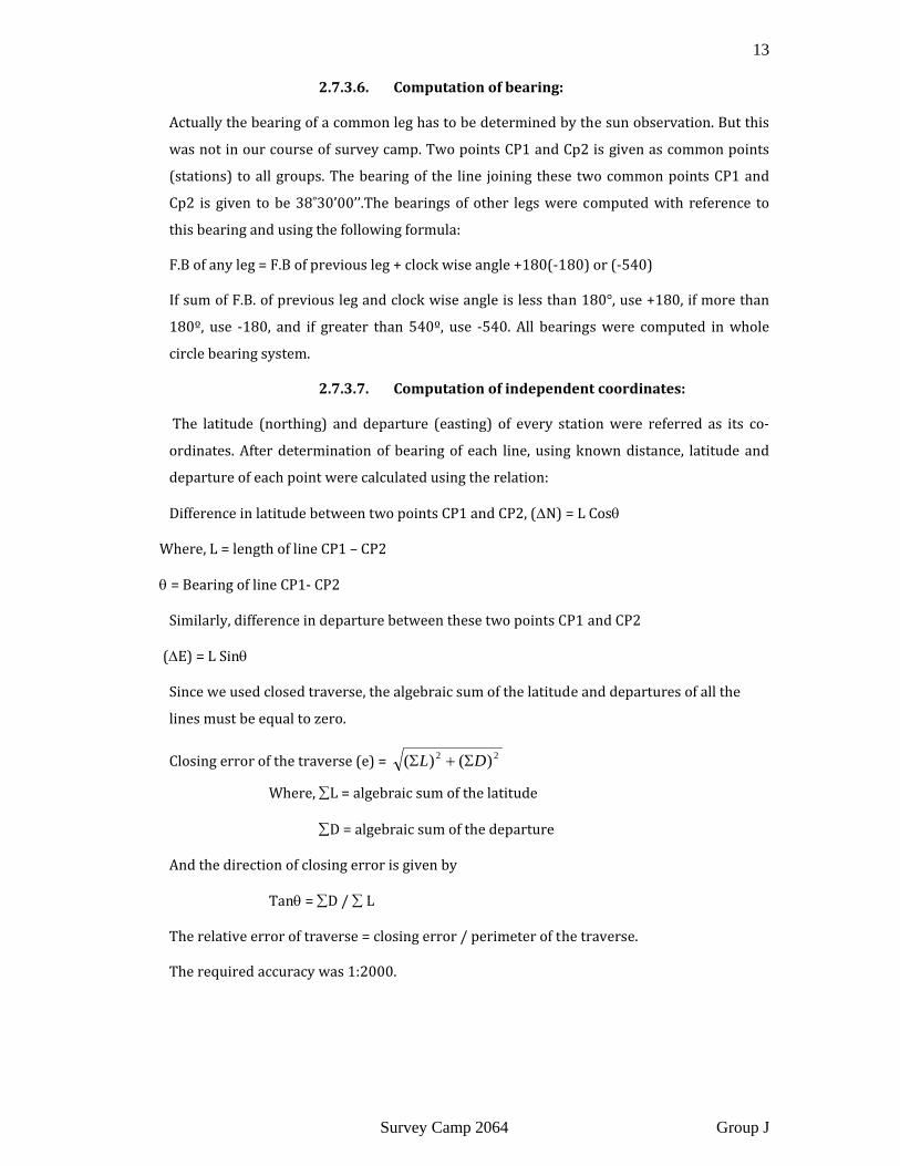
2.7.3.6. Computation of bearing:
Actually the bearing of a common leg has to be determined by the sun observation. But this
was not in our course of survey camp. Two points CP1 and Cp2 is given as common points
(stations) to all groups. The bearing of the line joining these two common points CP1 and
Cp2 is given to be 38˚30’00’’.The bearings of other legs were computed with reference to
this bearing and using the following formula:
F.B of any leg = F.B of previous leg + clock wise angle +180(‐180) or (‐540)
If sum of F.B. of previous leg and clock wise angle is less than 180°, use +180, if more than
180º, use ‐180, and if greater than 540º, use ‐540. All bearings were computed in whole
circle bearing system.
2.7.3.7. Computation of independent coordinates:
The latitude (northing) and departure (easting) of every station were referred as its co‐
ordinates. After determination of bearing of each line, using known distance, latitude and
departure of each point were calculated using the relation:
Difference in latitude between two points CP1 and CP2, (∆N) = L Cosθ
Where, L = length of line CP1 – CP2
θ = Bearing of line CP1‐ CP2
Similarly, difference in departure between these two points CP1 and CP2
(∆E) = L Sinθ
Since we used closed traverse, the algebraic sum of the latitude and departures of all the
lines must be equal to zero.
Closing error of the traverse (e) = 22 )()( DL Σ+Σ
Where, ∑L = algebraic sum of the latitude
∑D = algebraic sum of the departure
And the direction of closing error is given by
Tanθ = ∑D / ∑ L
The relative error of traverse = closing error / perimeter of the traverse.
The required accuracy was 1:2000.

14
Survey Camp 2064 Group J
Since there was some closing error, correction for latitude was necessary to make the
closing error zero i.e. the co‐ordinate must be same while closing the traverse at same point.
The co‐ordinate of succeeding station was calculated as:
Easting = easting of previous point + easting diff.
Northing = northing of previous point + northing diff.
2.7.3.8. Plotting the traverse using the coordinates
After the coordinates were calculated, they were plotted in a grid of 10‐by10 squares in the
scale of 1:1000 for the major traverse and 1:500 for the minor traverse.
Necessity of minor traverse:
When the details to be included in the map cannot be taken from the major traverse
stations then it becomes necessary to establish the control points near the detail so that it
can be observed properly and these stations are called minor stations. The minor traverse
should start from major station and should end at the major station too.
2.7.3.9. Sample Calculation: Reference: Table no:2.1
2.7.3.10. Final Coordinate Sheet: Reference Table no:2.2
2.8. MINOR TRAVERSE:
2.8.1 Introduction:
The traversed framework within the major traverse is called the minor traverse and was run to
detail the small area inside major traverse. All the vertical and horizontal controls were
transferred from the major traverse. Minor traverse legs were stretched in and out the detailing
area according to the requirement so as to achieve maximum information from that station
while performing plane tabling.
2.8.2 Methodology:
2.8.2.1 . Reconnaissance: The area given to us at the camp for detailing was lower zone of NEATC. As in the
case of major traversing reconnaissance was done before fixing minor stations. These minor stations are established in such a way that it covers each and every important detail.
2.8.2.2. Marking and Fixing Control Points:
After reconnaissance, it was concluded that extra four sub stations for detailing, that included 4 links (containing 16 stations in total) and 8 substations and four links joined to the major station forming a close minor traverse. So, 8 minor stations were fixed at the suitable place in such a way that indivisibility criteria between two stations are met.
2.8.2.3. Measurement of Traverse Legs:
As in the major traverse case, two‐way distance measurement was done. The accuracy required for the linear measurement was 1:1000.

15
Survey Camp 2064 Group J
2.8.2.4. Measurement of Interior Angles: On minor traverse stations, only one set of horizontal angles were taken.
Permissible Error = ±C√N minutes for traverse loop, where N is the no of stations. In the same case, error was distributed equally in all measured minor control points only. To determine the R.L. of minor control points, back sight was taken to the major traverse points. Intermediate sight was taken to the staff held at minor control points, and foresight was taken to the same or other major control points for closure. Accuracy =±25√K mm, where K is distance in k.m. Error found was within permissible limit. The error was distributed in each station according to Bowditch’s rule as discussed earlier. If e = total error in R.L. Then, correction =e*l/∑L where, l = length from initial station up to that station and ∑L = perimeter of traverse.
2.8.2.5. Bearing computation of the Traverse Legs: Bearing of traverse leg were calculated in
the same manner as in the major traversing, using the bearing of the major traverse line as known bearing of the initial line. Since the angular error was distributed previously, error in bearing calculation was checked.
2.8.2.6. Coordinate Computation of Minor Control Points:
Using the co‐ordinates of the major control point as given, co‐ordinates of the minor control points is determined in the same manner as in the major traversing. The traversing in this case was closed in the major traverse station and error was distributed in minor control points according to Bowditch’s Rule as done in major traversing.
2.8.2.7. Plotting of Minor Traverse Stations: As in the major traverse station, a full sheet
drawing was divided into 100 mm*100 mm grid and minor control points were plotted on the drawing sheet as a scale of 1:500.
2.8.3. Instrument Used: Theodolite
Staffs
Ranging rods
Tapes
Arrows
Pegs
Compass
2.8.4. Final Coordinate Sheet:

16
Survey Camp 2064 Group J
Reference: Table no. 2.2 2.8.5. Other observation and calculation Sheet:
Reference:
Linear Measurement: Table No.2.3 Horizontal Angular Obs. Sheet Major Traverse: Table No.2.4
Horizontal Angular Obs. Sheet Minor Traverse: Table No.2.5
Detailing : Table No.2.6
III. LEVELLING
3.1. INTRODUCTION:
Leveling is the branch of surveying, which is used to find the elevation of given points with respect to given, or assumed datum, to establish points at a given elevation or at different elevations with respect to a given or assumed datum. To provide vertical controls in topographic map, the elevations of the relevant points must be known so that complete topography of the area can be explored. Leveling was performed to determine the elevation (relative height) from a given datum.
3.2. Objective:
For the execution of engineering projects, such as railways, highways, canals, dams, water supply and sanitary schemes, it is very necessary to determine elevations of different points along the alignments of the proposed projects. Success of such projects depends upon accurate determination of elevations. Levelling is employed to provide an accurate net work of heights, covering the entire area of the project. Levelling is of prime importance to the engineers, both in acquiring necessary data for the design of the project and also during its execution. 3.3. Fly Leveling: 3.3.1. Introduction: Fly leveling is a leveling, which is done to find out the elevation of different points with respect to the standard benchmark. We performed the fly leveling from the TBM1
established by the survey department at Kharipati (way to Nagarkot) which was about 1500
meter away from NEATC. The R.L. of the TBM1 was 1348.122m and after carrying the fly
leveling the R.L. of TBM was 1336.834m but for the uniformity the survey instruction
committee provided the R.L. of TBM as 1336.864m.
17
Survey Camp 2064 Group J
3.3.2. Procedure:
A level machine was set up approximately midway between the benchmark and the
point, whose elevation was to be found by direct leveling. A back sight was taken on the staff
held at the benchmark.
Then,
H.I. = Elevation of B.M. + B.S.
By turning the telescope, another sight was taken on the staff held at the unknown point. At
that time, Elevation = H.I. – F.S. (or I.S.).
In our case before starting fly levelling we performed by the “Two Peg Test” on our
instrument.
3.3.3. Observation and Calculation:
Reference:
From Permanent BM to TBM: Table No.3.1
Level Transfer to Major Stations: Table No 3.2
Level Transfer to Minor Stations: Table No 3.3
3.3.4. Conclusion:
The R.L. of B.M. is given 1348.122 m (provided by the Survey instruction committee). Finally the R.L. of TBM at NEATC was determined by averaging all the R.L. calculated by each group, which was found to be 1336.864 m
3.4. Two Peg Test: 3.4.1. Introduction:
Two‐peg test is one of the methods of adjustment of the line of collimation,
which is done to compensate the collimation error of the leveling instrument. The line of
collimation of the telescope should be parallel to the axis of bubble tube. Therefore, the
adjustment of line of collimation is very necessary, and is of prime importance, since the
whole function of the level is to provide horizontal line of sight. This test is performed prior
to leveling work to confirm the leveling instrument is in the satisfactory condition fulfilling
the permissible limit.
The observations of the two‐peg test are as follows:
3.4.2. Observation:
18
Survey Camp 2064 Group J
T
T M
M B
B
A 25 m C 25m B
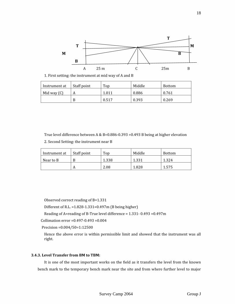
1. First setting: the instrument at mid way of A and B
True level difference between A & B=0.886‐0.393 =0.493 B being at higher elevation
2. Second Setting: the instrument near B
Observed correct reading of B=1.331
Different of R.L. =1.828‐1.331=0.497m (B being higher)
Reading of A=reading of B‐True level difference = 1.331‐ 0.493 =0.497m
Collimation error =0.497‐0.493 =0.004
Precision =0.004/50=1:12500
Hence the above error is within permissible limit and showed that the instrument was all right.
3.4.3. Level Transfer from BM to TBM:
It is one of the most important works on the field as it transfers the level from the known
bench mark to the temporary bench mark near the site and from where further level to major
Instrument at Staff point Top Middle Bottom Mid way (C) A 1.011 0.886 0.761
B 0.517 0.393 0.269
Instrument at Staff point Top Middle Bottom Near to B B 1.338 1.331 1.324
A 2.08 1.828 1.575

19
Survey Camp 2064 Group J
and minor traverse can be done easily. In other words we are establishing the control points
with the level transferred from the national survey department.
In the camp, level is transferred from to B.M. to T.B.M.
• Fore sight distance and backsight distance must be in nearly equal distance so as to
eliminate errors due to focusing, refraction and curvature. For maintaining equal
distance: eye judgment is used when the staff man fixed the fore sight distance with the
pacing.
• Three wire reading is taken. At each attempt mean value of three wire readings should
not differ by 0.002 m with the middle wire reading and was checked on the field.
• Fly levelling was run from T.B.M. to B.M. and back to the starting point so as to form loop.
Further correction was established two T.B.M. at the midway in the fly levelling.
• The permissible error was = ±25√ mm, where K is the distance in Kilometer of a loop.
• The R.L. of each staff station was found from rise and fall method.
• Closing error within the permissible limit was distributed to all staff stations according to their
length (station to staff distance)
3.4.3.1. Observation and Calculation:
Reference: (Table No 3.1)
3.4.4. Level transfer from T.B.M. to Major Traverse Station: The level transferred from B.M. to T.B.M. is now transferred to the Major traverse stations or the establishment of the major traverse stations is done with respect to R.L. of T.B.M...
Three wire reading was taken in each station. Fly levelling is done around the traverse and closed at T.B.M. R.L. is calculated by rise and fall method and error in per4missible limit was distributed.
3.4.4.1. Observation and Calculation: Reference: Table No 3.2
3.4.5. Level transferred from Major to Minor Traverse: It transferred the vertical control from major to the minor stations and from where Level was passed to each and every details point. This help in finding the R.L. of the ground points for contouring. By this means the Level was transferred to the every point on the site/Location where camp was launched. While performing this task, following points must kept in mind:
Three wire reading was taken in each station. Fly levelling could be started from R.L. of the known major station to the minor station and that to the known major station or from any major traverse station and closed that to the same station as it has vertical and horizontal control information.
The permissible error was= ±25√K mm, where K is in Kilometer. Error within the permissible limit was distributed proportionally to their lengths. 3.4.5.1. Observation and Calculation: Reference: Table No. 3.3
3.5. Reciprocal Levelling:
Reference: Chapter 7 bridge site survey (page: 57‐58)
20
Survey Camp 2064 Group J
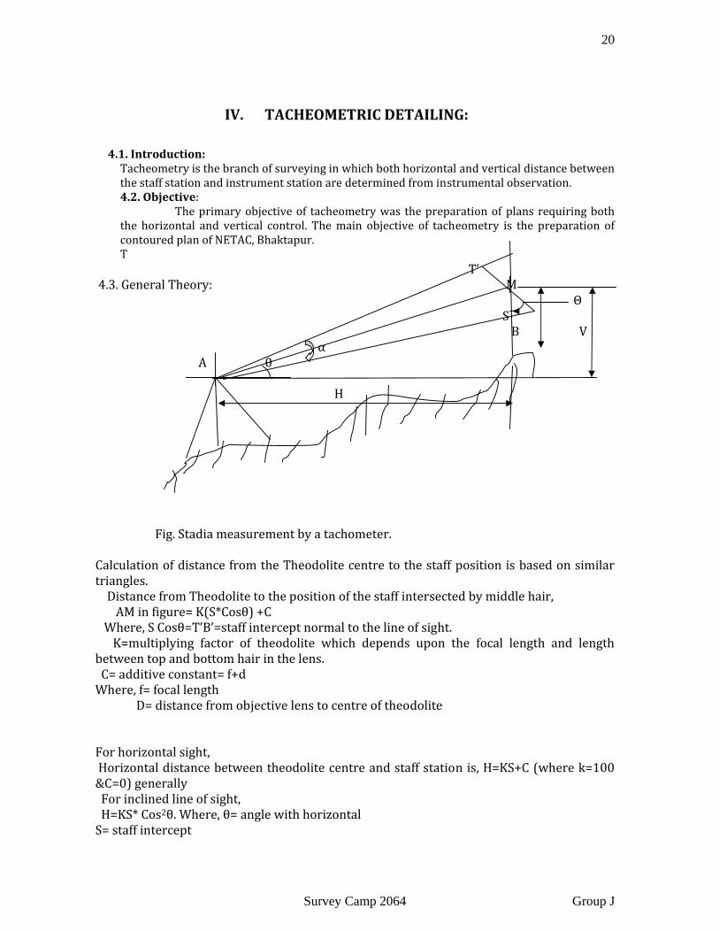
IV. TACHEOMETRIC DETAILING:
4.1. Introduction: Tacheometry is the branch of surveying in which both horizontal and vertical distance between the staff station and instrument station are determined from instrumental observation.
4.2. Objective: The primary objective of tacheometry was the preparation of plans requiring both the horizontal and vertical control. The main objective of tacheometry is the preparation of contoured plan of NETAC, Bhaktapur. T
T’ 4.3. General Theory: M Θ S
B V α A θ H
Fig. Stadia measurement by a tachometer.
Calculation of distance from the Theodolite centre to the staff position is based on similar triangles. Distance from Theodolite to the position of the staff intersected by middle hair, AM in figure= K(S*Cosθ) +C Where, S Cosθ=T’B’=staff intercept normal to the line of sight. K=multiplying factor of theodolite which depends upon the focal length and length between top and bottom hair in the lens. C= additive constant= f+d Where, f= focal length D= distance from objective lens to centre of theodolite For horizontal sight, Horizontal distance between theodolite centre and staff station is, H=KS+C (where k=100 &C=0) generally For inclined line of sight, H=KS* Cos2θ. Where, θ= angle with horizontal S= staff intercept
21
Survey Camp 2064 Group J
For vertical distance, from centre of theodolite to the middle hair position in staff. V=KS Cosθ*Sinθ= (KS Sin2θ)/2 If horizontal angle is taken, H=KS Sin2θ and V=1/2*KS Sin2θ
4.3. Methodology: 4.3.1. Measurement and Data:
Initially the Theodolite is set on a station and necessary adjustment is done. Detailing of the survey area is carried out by setting horizontal angle to 0˚0’0’’ to the corresponding station.
The object is sighted and staff intercept ( top, middle and bottom wire reading ) is Observed and corresponding vertical angle (VCR) and horizontal angle (HCR) is read.
4.3.2. Field Procedure: 1. Zero angles are set at the back sight to the traverse station. 2. Staff reading is taken i.e., bottom, middle and top at the necessary
position. 3. Staff man is allowed to go to the next position. 4. Vertical and horizontal angles are taken. 5. Height of instrument should be taken initially.
Now, the horizontal and vertical distances are obtained using formulas. Then by use of horizontal angles and distance we can plot the necessary details. The vertical distance is reduced to calculate the RL of staff stations which will serve for rough contouring in the topographic map.
4.3.3. Calculation:
If S = Stadia reading (Top wire – Bottom wire)
Θ = Vertical angle (V.C.R. ‐ 90˚ if V.C.R.>90˚ & 90˚‐V.C.R. if V.C.R. <90˚
H = Horizontal distance then,
H = 100*S*Cos2θ + C *Cosθ
And R.L. of staff point = R.L. of instrument station + height of instrument ±V (HTanθ or 50*S*Sin2θ + C Sinθ+ C Sinθ) – Central wire reading.
Note: C= 0 for our instrument, V is taken positive when vertical angle is angle of elevation ( Less than 90˚) and V is taken as negative when vertical angle is angle of depression.
4.3.4. Accuracy and Precision:
The average of sum of upper wire reading and bottom wire reading should be equal to
the central wire reading for the accurate result.
i.e. (Top+ Bottom)/2 = center
22
Survey Camp 2064 Group J
4.3.4. Instrument:
Theodolite
Staffs
Ranging rods
Tapes
Arrows
Pegs
Compass
4.4. Contouring:
The delineation of any property in map form by constructing lines of equal values of
that property from available data points is known as contour mapping. A topographic map,
for example, reveals the relief of an area by means of contour lines that represent elevation
values; each such line passes through points of the same elevation. The method is not wholly
objective because two investigators may produce somewhat different maps whenever
interpolation between data points is necessary for construction of the contours. The
availability of plotting devices in recent years has permitted mapping by computer, which
reduces the effect of human bias on the final product.
Contour lines are imaginary lines exposing the ground features and joining the points of
equal elevations. The map with contour line relief is a topographic map. The relief interval
between two consecutive contour lines is called the contour interval and is fixed. For the
contour plan, the contour interval is kept constant and the provided contour interval was
1m.
4.4.1. Methods of locating Contours
The methods of locating contours depend upon the instrument used. In general there are
main two basic field methods of locating contours. They are:
i. The direct method. & ii. The indirect method.
i. The direct method: In the direct method, the contours to be plotted are actually traced
23
Survey Camp 2064 Group J
on the ground. Only those points are surveyed which happen to be plotted. This method is slow and tedious. Here, contour map is prepared on the field.
ii. The indirect method
In the indirect method, some suitable guide points are selected and surveyed. The guide
point need not necessarily be on the contours. These guide points, having been plotted serve
as a basis for the interpolation of contours. This method was used to locate the contours.
4.4.2. Interpolation of Contours:
Contour interpolation is the process of spacing the contours proportionately between the
plotted ground points established by indirect methods. The methods of interpolation are
based on assumption that the slope of ground between the two points is uniform. There are
three methods of interpolation. They are:
i. By estimation:
The method of estimation is not very precise. In this method contours are
interpolated between two known R.L. by eye judgment. So, the accuracy of this method
is low compared to other two methods. The accuracy of this method depends upon the
experience of the surveyor
ii. By arithmetic calculations:
The arithmetic calculation method was used while interpolation of contours. It is
accurate method and the positions of contour points between the guide points are
located by simple arithmetic calculation.
iii. By graphical method:
The graphical method is one of the methods of contour interpolation. The accuracy
of this method is high compared to the estimation method but this method is long and
tedious.
Detailing: In order to plot the topographic map in the given scale, detailing was done by using
tacheometry from minor traverse plotted on the drawing sheet. From the tacheometry the
horizontal and the vertical distance were observed. Those distances can be used to plot any
details on site and the contour can also be drawn by calculating the R.L. of each and every
points.
Here the distances are calculated as follows:
H = KS (Cosθ)²
V = KS (Sin2θ)
Where K = 100

24
Survey Camp 2064 Group J
S= (top reading – bottom reading)
θ = vertical angle
Now the R.L. of the staff station is calculated as follows
R.L. of staff station = R.L. of instrument station + HI +V – Middle wire reading
To know the use of telescopic alidade, few detailing were done using it. The alidade used
was self‐reducing type. It is the direct method of detailing in the field. Here the horizontal
and vertical distances are calculated on the spot and then plotted immediately. The
calculations of telescopic alidade may be summarized as
V= (top – bottom)*100
H= (Middle – bottom)*100*f (factor)
R.L. of staff station = R.L. of instrument station + HI + V – Middle reading
Field Verification After the completion of the calculation of major and minor coordinates and plotting
them in the scale of 1:500 (Minor traverse) and 1:1000 (Major traverse) with the help of
gridlines, it has to be verified in the field with the help of telescopic alidade by plane table
method.
4.5. Comments And Conclusion:
Since NEATC area has a lot of variation in regard to the altitude, type of vegetation and other
details within itself, it is a very ideal place for topographical surveying. We were able to
familiarize ourselves with the different practical approaches applied in the actual field
condition. We experienced the difference between working in a smaller area and a larger
one. Along with gaining the lots of confidence regarding the use of instrument, we also felt
the responsibility of planning, executing and implementing a project. On the whole we
experienced the value of teamwork and mutual coordination in the execution of any project.
4.6. Observation And calculation:
Reference: Table 4.1. (Detailing sheet)
25
Survey Camp 2064 Group J
V. ORIENTATION
5.1. To determine The Position of Unknown Point By The Method Of
Intersection :
5.1.1. Introduction: Intersection is the process of determining the position of an unknown and inaccessible
Position, with the help of known points, by setting instruments at the known points. In this method, the instrument is set only at the known points. The vertical angle and horizontal angle from each station to the known point is noted with the help of which the position of unknown points is determined.
5.1.2. Objective:
The main objective of intersection is to determine the co‐ordinate of the unknown point
which may or may not accessible, with the help of the three known points.
5.1.3. Instruments Required:
Theodolite
Ranging rods
Arrows

26
Survey Camp 2064 Group J

27
Survey Camp 2064 Group J

28
Survey Camp 2064 Group J

29
Survey Camp 2064 Group J

30
Survey Camp 2064 Group J

31
Survey Camp 2064 Group J

32
Survey Camp 2064 Group J

33
Survey Camp 2064 Group J

34
Survey Camp 2064 Group J

35
Survey Camp 2064 Group J

36
Survey Camp 2064 Group J

37
Survey Camp 2064 Group J

38
Survey Camp 2064 Group J
VI. CURVES
39
Survey Camp 2064 Group J
6.1. INTRODUCTION:
Curves are generally used on highways and railways where it is necessary change the
direction of motion. A curve may be circular, parabolic or spiral and is always tangential to
straight directions. The main objective of curve setting in the highway is to allow the
vehicles turn their direction safely and smoothly so that the passenger doesn’t fill any jerk
and difficulty.
6.2. SIMPLE CIRCULAR CURVES
A simple circular curve is the curve, which consists of a singular arc of a circle. It is
Tangential to both the straight lines. Setting out of curves can be done by two methods
depending upon the instrument used.
i. Linear method: ‐ In this method, only a chain or tape is used when a high degree of
accuracy is not required and the curve is short.
ii. Angular method: ‐ In this method, an instrument like theodolite is used with or without
chain or tape. Before a curve is set out, it is essential to locate the tangent points of
intersection, points of curve and points of tangents.
The linear method adopted for setting out curve in field was ordinate from long chord. The
angular method adopted in field was Rankine’s method.
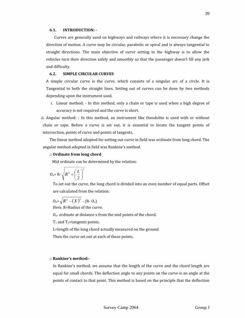
o Ordinate from long chord
Mid ordinate can be determined by the relation:
Oo= R‐2
2
2⎟⎠⎞
⎜⎝⎛+
LR
To set out the curve, the long chord is divided into an even number of equal parts. Offset
are calculated from the relation:
Ox= ( )22 XR − ‐ (R‐ Oo) Here, R=Radius of the curve.
Ox= ordinate at distance x from the mid points of the chord.
T1 and T2=tangents points.
L=length of the long chord actually measured on the ground.
Then the curve set out at each of these points.
o Rankine’s method:
In Rankine’s method, we assume that the length of the curve and the chord length are
equal for small chords. The deflection angle to any points on the curve is an angle at the
points of contact to that point. This method is based on the principle that the deflection
40
Survey Camp 2064 Group J
angle to any points on a circular curve is measured by one half the angles subtended by
the arc on P.C. to that point.
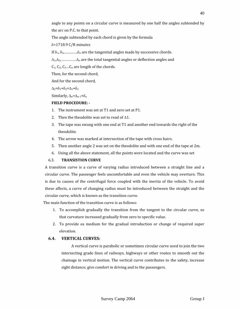
The angle subtended by each chord is given by the formula
δ=1718.9 C/R minutes
If δ1, δ2,………….δn are the tangential angles made by successive chords.
∆1,∆2,……………∆n are the total tangential angles or deflection angles and
C1, C2, C3…Cn are length of the chords.
Then, for the second chord,
And for the second chord,
∆2=δ1+δ2=∆1+δ2
Similarly, ∆n=∆n‐1+δn
FIELD PROCEDURE:
1. The instrument was set at T1 and zero set at P1.
2. Then the theodolite was set to read of ∆1.
3. The tape was swung with one end at T1 and another end towards the right of the
theodolite.
4. The arrow was marked at intersection of the tape with cross hairs.
5. Then another angle 2 was set on the theodolite and with one end of the tape at 2m.
6. Using all the above statement, all the points were located and the curve was set
6.3. TRANSISTION CURVE
A transition curve is a curve of varying radius introduced between a straight line and a
circular curve. The passenger feels uncomfortable and even the vehicle may overturn. This
is due to causes of the centrifugal force coupled with the inertia of the vehicle. To avoid
these affects, a curve of changing radius must be introduced between the straight and the
circular curve, which is known as the transition curve.
The main function of the transition curve is as follows:
1. To accomplish gradually the transition from the tangent to the circular curve, so
that curvature increased gradually from zero to specific value.
2. To provide ea medium for the gradual introduction or change of required super
elevation.
6.4. VERTICAL CURVES:
A vertical curve is parabolic or sometimes circular curve used to join the two
intersecting grade lines of railways, highways or other routes to smooth out the
chainage in vertical motion. The vertical curve contributes to the safety, increase
sight distance; give comfort in driving and to the passengers.

41
Survey Camp 2064 Group J
A grade, which is expressed as percentage or 1 vertical in N horizontal, is
said to be upgrade or +ve grade when elevation along it increases, while it is
termed as downgrade or –ve grade when the elevation decreases along the
direction of motion.
Assumption for calculating data which are required for setting out of Vertical
Curve:
B (apex)
‐ g 2%
+g1% P(x,y) B1 (vertex)
l y l
T1 x B2 T2 EVC
BVC L
Fig. Vertical curve.
Length of vertical curve = length of two tangent
So BT1 +Bt2 = 2l = T1B1+B1T2
Curve is assumed to be equally long on either side of the vertex. So,
T1B1=T2B2 =l
Length of vertical curve, L = no of chains, where r = rate of grade per
chain length.
Chainage of T1 = chainage of B –BT1 (l)
Chainage of T2 = chainage of B + BT2 (l)
R.L. of T1 = R.L. of B ±
R.L. of T2 = R.L. of B±
R.L. of B2 = ½(R.L. of T1 + R.L. of T2)
R.L. of B1 = ½ ( R.L. of B + R.L. of B2)
General formula for R.L. of any point is given by:
R.L. of Point i.e. P (Y) =
+ + R.L. of BVC
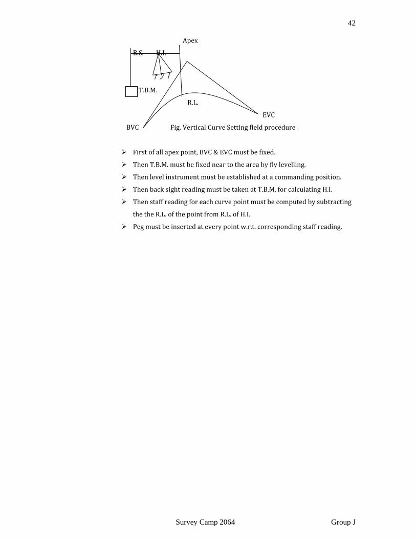
Method Of Setting Out Of Vertical Curve:
42
Survey Camp 2064 Group J
Apex
B.S. H.I.
T.B.M.
R.L.
EVC
BVC Fig. Vertical Curve Setting field procedure
First of all apex point, BVC & EVC must be fixed.
Then T.B.M. must be fixed near to the area by fly levelling.
Then level instrument must be established at a commanding position.
Then back sight reading must be taken at T.B.M. for calculating H.I.
Then staff reading for each curve point must be computed by subtracting
the the R.L. of the point from R.L. of H.I.
Peg must be inserted at every point w.r.t. corresponding staff reading.

43
Survey Camp 2064 Group J

44
Survey Camp 2064 Group J
TRANSITION CURVE:

45
Survey Camp 2064 Group J

46
Survey Camp 2064 Group J

47
Survey Camp 2064 Group J

48
Survey Camp 2064 Group J
49
Survey Camp 2064 Group J
VII. ROAD ALIGNMENT SURVEY
7.1. Introduction
Roads are especially prepared ways between different places for the use of vehicles and
peoples. In country like Nepal, where there is less chance of airways and almost negligible chance
of waterway, roads form the major part of the transportation system. It is an important aspect in
the development of transportation network for the topographical mapping while the knowledge of
longitudinal section as well as cross sections at certain intervals of the road are essential. Also the
density of traffics should be considered before designing the road. The roadside survey was
conducted at NEATC premises .The length of the surveyed road was about 782 m.
7.2. Objectives
Road alignment survey was done to accomplish the following objectives:
To lay out the road joining from the southern part of the NEATC to the
main entrance at northern part.

50
Survey Camp 2064 Group J
To choose the best possible route for the road such that there were a
minimum of number of intermediate points (I. P.) there by decreasing the
number of turns on the road.
To design smooth horizontal curves at points where the road changed its
direction in order to make the road comfortable for the passengers and the
vehicles traveling on it.
To take the sufficient data of the details including the spot height around
the road to prepare the topographical map of the area, cross section of the
road segment hence making it convenient to determine the amount of cut
and fill required for the construction of the road.
7.3. Norms (Technical Specification)
The road has to be designed for a width of 5 meter and length of 500m.
If the external deflection on the road is less then 3º the curve need not to be
fitted.
Simple horizontal curve has to be laid out where the road changed its
direction, determining and pegging the three points on the curves – the
beginning of the curve, mid of the curve and the end of the curve along the
central line of the road.
The radius of the curve should be greater then 12m.
The gradient of the road has to be maintained below 7%.
Cross‐section should be taken at the interval of 15 to 20m and also at the
beginning, middle and end of the curve along the central line of the road.
Plan of the road should be prepared in the scale of 1:500.
L‐ Section of the road has to be plotted on the scale of 1:500 on X‐ axis and
1:100 vertically.
The cross section of the road should be plotted on the scale of 1:100 for both
the axis.
7.4. Instruments required
Theodolite
Staff
Tape
51
Survey Camp 2064 Group J
Level
Tripod
Arrows
Hammer
Compass with stand
7.5. METHODOLOGY
7.5.1. Reconnaissance
The Reconnaissance survey was carried out starting from the point just crossing the
river to the point where the existing road met the market place. Pegging was done at
different places and the possible I.P. were also numbered and pegged. The condition of
indivisibility was checked at each step.
7.5.2. Horizontal Alignment
The location of the simple horizontal curve were determined carefully considering
factors like the stability of the area, enough space for the turning radius etc. The I.P. was fixed
so that the gradient of the road at any place was less than 7‐10%. After determining the I.P
for the road, theodolite was stationed at each I.P. and the deflection angles measured. The
distance between one I.P. and another was measured by two way taping.
The horizontal curve was set out by angular method using theodolite at I.P. and tape.
The radius of the curve was fixed first, assuming it to be more then m. Then for that radius,
the tangent length and apex distance of the curve were calculated using the following
formulas:
Tangent Length = 2
tan ∆R
Apex Distance = ⎟⎠⎞
⎜⎝⎛ −
∆ 12
secR
Length of the Curve = 180∆Rπ
Where ∆ = External deflection angle
After performing the necessary calculation, the points T1 and T2 were fixed at a
distance equal to tangent length from the I.P. using a tape. Then the line bisecting the
internal angle at the I.P. was found out with the help of a theodolite. And on this line,
a peg was driven at mid of curve at a distance equal to the apex distance from the I.P.
Then the necessary calculation was done, thus giving the required numerical values
of different parameters.
7.5.3. Curve fitting with inaccessible
52
Survey Camp 2064 Group J
The same procedure was followed for the two curves designed on the road and
hence chainage of all the points was calculated.
7.5.4. Leveling
The method of fly leveling was applied in transferring the level from the given B.M.
to all the I.P., beginnings, mid points and end of the curve as well as to the points
along the center line of the road where the cross section were taken. After
completing the work of one way leveling on the entire length of the road, fly leveling
was continued back to the B.M making before and after forming the loops should be
less than 25 K mm, where k is total loop distance in km.
7.5.5. Longitudinal section
The L‐section of the road is required to the road engineer an idea about the nature of
the ground and the variation in the elevation of the different points along the length
of the road an also to determined the amount of cutting and filling required at the
road site for maintaining a gentle slope. In order to obtain the data for L‐Section,
Staff reading was taken at a point at 25m intervals along the central line of the road
with the help of a level by the method of fly leveling. And thus after performing the
necessary calculation the level was transferred to all those point with respect R.L. of
the given B.M. Then finally the L‐Section of the road was plotted on a graph paper on
a vertical scale of 1:100 and a horizontal scale of 1:500.
7.5.6. CrossSection
Cross Section at different points is drawn perpendicular to the longitudinal section
of the road on either side its center line is order to present the lateral out line of the
ground. Cross Section is also equally useful in determining the amount of cut and fill
required for the road construction. The cross sections were taken at 25m intervals
along the center line of the road and also at point where there was a sharp change in
the elevation. While doing so, the horizontal distance of the different points from the
center line measured with the help of a tape and vertical height with a measuring
staff. The R.L. was transferred to all the points were performing the necessary
calculation and finally the cross section at different section were plotted at graph
paper on a scale of 1:100 both vertical and horizontal.
7.5.7. Calculations and plotting
After the work of taking the data was completed, all the necessary calculations were
done and tabulated in order to compute the Chainage of the different distinct points
of the road using the following relation:
Chainage of beginning of curve, T1=Chainage of I.P.‐Tangent length
Chainage of mid point of curve, M=Chainage of T1‐1/2*curve length
53
Survey Camp 2064 Group J
Chainage of end of curve, T2= Chainage of T1+Curve length
Similarly,
Chainage of an I.P. = Chainage of previous I.P. +I.P. to distance
The R.L. of the different points was also computed using this formula.
R.L. of a point =R.L. of station + Height of instrument + H* Tan ѳ‐Mid wire reading
Where θ =Vertical Angle
Hence, with the required calculation data regarding the road site in hand, the plan
was plotted on a scale of 1:500,L‐Section on a graph paper on a scale of 1:500
horizontal and 1:100 vertical and the cross section at different points also on a
graph paper on a scale of 1:100(both vertical and horizontal).
All the data, calculation (in a tabulated from) and the drawing of the necessary plan,
longitudinal section and the cross section of the road are presented here with this
report.
7.5.8. Observation And Calculation: Reference:
Co‐Ordinate Sheet (Gales Table): Table No. 7.1 Chainage And IP calculation Sheet: Table No. 7.2 Level Transfer To IPs: Table No. 7.3 Detailing Sheet: Table No. 7.4
7.5.9. Comments And Conclusion
In spite of the different kinds of obstacles in the field, our group was successful in
completing the fieldwork as well as the office work in time. In field, we had spent quite
some time discussing the route of the road and also in designing the two curves, which led
to good results. However, the entire group members were very cautious and tried their
best to get error free data and calculations.
Moreover, after performing this road alignment survey, we were able to build confidence
in designing roads at difficult terrain taking factors like economy, convenience and its use
into consideration. We believe that such a work will be a lot of help for us in
understanding the actual situation while undertaking actual design and construction work

54
Survey Camp 2064 Group J
in the future and we hope that organizes such useful field trips of the entire subject
frequently.
VIII. BRIDGE SITE SURVEY
8.1. Introduction
Bridges are the structures that are constructed with the purpose of connecting the two
places separated by rivers, streams, valleys or seas. The bridges are the network provider
for the different roads. The bridges are usually a part of road, making the road shorter and
hence economical. In Nepal where there are lots of uneven lands and plenty of rivers, the
bridges are almost the economical and efficient way to joint the two places by road in a
convenient way. The bridges are that part which connects the two impossible points, which
may be separated by some river or gorge.
Punyamata Khola was the site provided to us for the bridge site. It is situated at about 3
kilometers south of Banepa chowk. Out of 15 days of our total survey camp, 2 days were
55
Survey Camp 2064 Group J
assigned for the bridge site and road site survey. Out of these three days we had to complete
the work of our bridge site in one and a half days.
8.2. Objectives
The bridge site survey was carried with the following objectives:
To develop an idea for selection of bridge axis over the river considering the factors
like convenience, economy, and geological stability.
To use the method of triangulation and reciprocal leveling, performing the necessary
calculations to calculate the length of the bridge axis using sine rule.
To prepare the topographical map of the area, cross section of the river at certain
intervals and the longitudinal section of the river including the details of the various
features and structures at the upstream and the downstream of the bridge axis.
To know the nature of the river like its discharge, velocity of flow, bed slope, higher
flood level etc.
8.3. Brief description of the site:
The site for the bridge site survey was selected on the way to Panauti at Punyamata
Khola.
The site consists of the mild vegetation including the cultivated land and few houses. To
prevent the high flood level and its devastation to land, the gabion wall has been placed at
the bank of the river as shown in the map. There is also a small bridge, which assists only
the light vehicles.
8.4. Hydrology, Geology & Soil:
The climatic condition of the Kathmandu Valley is sub‐tropical and characterized
by a seasonal pattern of monsoon that occurs mainly during rainy season from June
to September. The rainfall is generally of least during winter season. Another
important feature of this pattern is largely variation in the amount as well as on
place also.
8.5. Norms (Technical Specifications)
The following norms were followed while performing the bridge site survey:
5. Control point fixing as well as determining the length of the bridge axis had to be done by the
method of triangulation. While forming triangles, proper care had to be taken such that the
triangles were well conditioned, i.e. none of the angles of the triangle were greater than 120° or
less than 30°.
6. The triangulation angle had to be measured on two sets of readings at 0° and 90° by theodolite
and the difference between the mean angles of two sets of readings had to be within a minute.
56
Survey Camp 2064 Group J
7. Transferring the level from one bank to another bank had to be done by the method of
reciprocal leveling.
8. The scale for plotting the topographical map was given to be 1:500 In order to plot the
longitudinal section of the river; data had to be taken along the riverbed up to 120 m upstream
and 60m downstream. The plot for the longitudinal section along the flow line had to be done in
a scale of 1:100 for vertical and 1:500 for horizontal. And for the cross section use the scale of
1:100 for both horizontal and vertical or 1:100 for vertical and 1:200for horizontal.
8.6. Instruments Required
The instruments required in the survey during the preparation of topographic map are as
follows:
o Theodolite o Staffs o Ranging rods o Tapes o Leveling instruments o Compass o Pegs o Marker o Tripod o Arrow
8.7. Methodology
8.7.1. Reconnaissance and site selection
The bridge site survey was done at Punyamata Khola. The first step, the
reconnaissance was done for the entire area where the bridge was to be located and
the location of the bridge axis was chosen. The site for the bridge was selected at a
location that was a continuation of the straight portion of the existing road.
8.7.2. Fixing the stations
After the completion of the recce, six stations were fixed which included the two
points of the bridge axis and it also included two points on the left hand side and two
points on the right hand side on upstream and down stream respectively. The length
of the two baselines was measured with the tape with high precision of 1:2000. The
horizontal angles were measured and the coordinates of the control points were

57
Survey Camp 2064 Group J
calculated with the help of the coordinates of temporary benchmark (T.B.M.), which
was (1000.000, 1000.000, and 1456.243).
8.7.3. Topographic Survey
For the topographic survey of the bridge site triangulation was done. First the bridge
axis was set and horizontal control stations were fixed on either side for detailing.
All together six stations were fixed, with three on each bank. Thus traverse was
formed running across the river, covering the distance of 120m upstream and 60m
downstream. The interconnecting triangles were formed and angles were
measured with theodolite. The bridge axis length or span was calculated by solving
the triangles using the sine rule. Thus the horizontal control was set out.
For vertical control, the level was transferred from the TBM at the bridge near the
site by fly leveling and RL was transferred to the stations on the next bank by
reciprocal leveling. For the same bank direct level transfer method was used. For the
RL transfer for other stations then the bridge axis points the tachometric formulas
are used. The checks should be provided as far as possible. All the details were taken
by the tachometric method.
8.7.4. Longitudinal Section:
The triangulation was to determine the length of the bridge axis and to fix the
control points for detailing. The triangular stations were setup keeping in mind the
necessity of the well‐conditioned triangle. The longitudinal section of the river is
required to give an idea about the bed slope, nature of river bed, and variation of the
elevation of the different points along the length of the river. Keeping the instrument
in the control station on the river bank, the staff readings were taken at different
points along the center line of the river at an interval of 20m up to 120m upstream
and 60m downstream of the river. The elevations of the control points being known
previously, the RLs of different points at the center lines was calculated using the
tachometric formulas. Finally the L‐ section (profile) of the river bed was plotted on
the graph paper with the scale of 1:100 in Y‐axis and 1:500 in X‐axis. The graph is
attached here with the report.
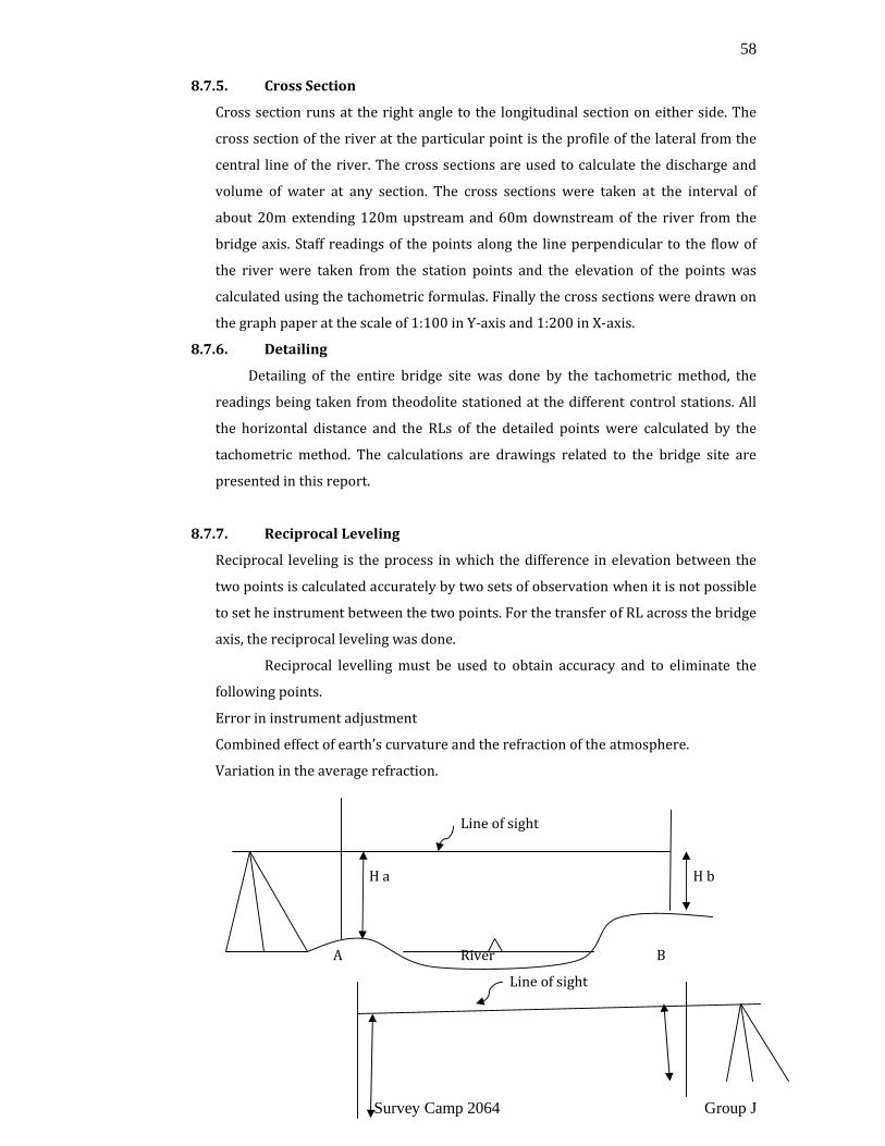
58
Survey Camp 2064 Group J
8.7.5. Cross Section
Cross section runs at the right angle to the longitudinal section on either side. The
cross section of the river at the particular point is the profile of the lateral from the
central line of the river. The cross sections are used to calculate the discharge and
volume of water at any section. The cross sections were taken at the interval of
about 20m extending 120m upstream and 60m downstream of the river from the
bridge axis. Staff readings of the points along the line perpendicular to the flow of
the river were taken from the station points and the elevation of the points was
calculated using the tachometric formulas. Finally the cross sections were drawn on
the graph paper at the scale of 1:100 in Y‐axis and 1:200 in X‐axis.
8.7.6. Detailing
Detailing of the entire bridge site was done by the tachometric method, the
readings being taken from theodolite stationed at the different control stations. All
the horizontal distance and the RLs of the detailed points were calculated by the
tachometric method. The calculations are drawings related to the bridge site are
presented in this report.
8.7.7. Reciprocal Leveling
Reciprocal leveling is the process in which the difference in elevation between the
two points is calculated accurately by two sets of observation when it is not possible
to set he instrument between the two points. For the transfer of RL across the bridge
axis, the reciprocal leveling was done.
Reciprocal levelling must be used to obtain accuracy and to eliminate the
following points.
Error in instrument adjustment
Combined effect of earth’s curvature and the refraction of the atmosphere.
Variation in the average refraction.
Line of sight
H a H b
A River B
Line of sight
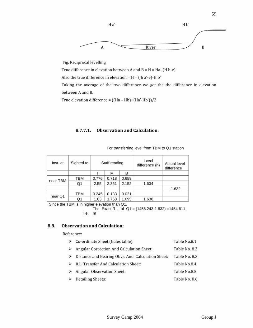
59
Survey Camp 2064 Group J
H a’ H b’
A River B
Fig. Reciprocal levelling
True difference in elevation between A and B = H = Ha‐ (H b‐e)
Also the true difference in elevation = H = ( h a’‐e)‐H b’
Taking the average of the two difference we get the the difference in elevation
between A and B.
True elevation difference = ((Ha – Hb)+(Ha’‐Hb’))/2
8.7.7.1. Observation and Calculation:
For transferring level from TBM to Q1 station
Inst. at Sighted to Staff reading Level difference (h) Actual level
difference T M B
near TBM TBM 0.776 0.718 0.659 Q1 2.55 2.351 2.152 1.634
1.632
near Q1 TBM 0.245 0.133 0.021 Q1 1.83 1.763 1.695 1.630
Since the TBM is in higher elevation than Q1.
i.e. The Exact R.L. of Q1 = (1456.243-1.632) =1454.611 m
8.8. Observation and Calculation:
Reference:
Co‐ordinate Sheet (Gales table): Table No.8.1
Angular Correction And Calculation Sheet: Table No. 8.2
Distance and Bearing Obvs. And Calculation Sheet: Table No. 8.3
R.L. Transfer And Calculation Sheet: Table No.8.4
Angular Observation Sheet: Table No.8.5
Detailing Sheets: Table No. 8.6

60
Survey Camp 2064 Group J
8.9. Computation and Plotting
The bearing of TBM from one of the axis station was taken and the detailing of
the TBM was also done from the same station. By the help of these two the bearing
of all the lines (outer frame joining the control points) was determined. The length
of the two base lines was measured with the tape and the rest is calculated by using
the sine rule in different triangles. From the bearing and the length the coordinates
of all the stations were calculated with reference to the coordinate of TBM.
The horizontal and vertical distances were calculated using the tachometric
formulas.
The formula for the horizontal distance is,
H =KSCos2θ
The formula for the vertical distance is,
V = 2K S Sin2θ
Where K = 100
S = Staff intercept = (Top reading – Bottom reading)
After the completion of all the calculation and the computation, the plotting of
topographic map was done in the scale of 1:500 with the help of proper gridlines.
Then the L‐section and cross sections were done.
8.10. Comments and Conclusion
Bridge site provided to us was quite steep area so it was difficult to take the staff
readings the different points that were required, so all the necessary data were assumed.
After the completion of the bridge site survey and calculation it was found that the bridge
span was 58.153m. The bridge site survey provided great knowledge to us about the
construction of the bridge. After the completion of the bridge site survey we had the idea
about the selection of the bridge axis. It also helped us to know the value of teamwork
with which the completion of the work was not possible. Finally, all maps, graphs and all
the necessary calculations are attached here with the report.
61
Survey Camp 2064 Group J
IX. CONCLUSION AND RECOMMENDATIONS
9.1. Conclusion
The two weeks of surveying have been most educative. As far as field knowledge is
concerned, the traversing and the detailed surveying performed at NEATC, Kharipati helped
to understand better the fundamental principle of surveying working from the whole to
part. The vertical control of the major traverse stations was selected with high degree of
precision. Hence the degree of accuracy achieved was also of great order.
62
Survey Camp 2064 Group J
The topographical survey done at the Punyamata Khola was able to impart a preliminary
knowledge on how to select the bridge axis for the construction of the bridge and the
collection of the data for performing the preliminary office work for bridge construction.
Road survey done at the same site was also helpful for the knowledge required on the
design of road and also and setting the curve.
The selection of members for each group for the survey camp were done by teachers with
the objective that each student should adjust with every other student and know the value
of teamwork. And the objective was greatly fulfilled.
9.2. Recommendations
Survey camp was almost good and also it gives a lot of experiences and helped us to build
up the confidence. Due to limited time, we had to perform every work in hurry due to which
some error were committed in the field but it may be due to instrumental error, whatever it
may be, the main thing is that all the errors were in the permissible limits and were
corrected or distributed. Rather the table work was more than the fieldwork. All the group
members were equally active and co‐operative so we completed our work in time.
X. BIBLIOGRAPHY
1. A Text Book of Surveying. (R.Agor)
2. A Text Book of Surveying (Vol I & II). (Dr. B.C. Purnima)

63
Survey Camp 2064 Group J
3. A Text Book of Surveying (Vol I & II). (David Clark)
4. Surveying (Vol I & II). S.K. Duggal
5. Surveying A. Bannister & S. Raymond
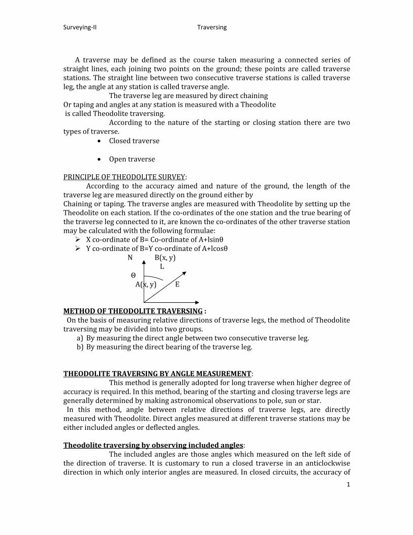
Surveying‐II Traversing
1
A traverse may be defined as the course taken measuring a connected series of straight lines, each joining two points on the ground; these points are called traverse stations. The straight line between two consecutive traverse stations is called traverse leg, the angle at any station is called traverse angle. The traverse leg are measured by direct chaining Or taping and angles at any station is measured with a Theodolite is called Theodolite traversing. According to the nature of the starting or closing station there are two types of traverse.
• Closed traverse
• Open traverse
PRINCIPLE OF THEODOLITE SURVEY: According to the accuracy aimed and nature of the ground, the length of the traverse leg are measured directly on the ground either by Chaining or taping. The traverse angles are measured with Theodolite by setting up the Theodolite on each station. If the co‐ordinates of the one station and the true bearing of the traverse leg connected to it, are known the co‐ordinates of the other traverse station may be calculated with the following formulae:
X co‐ordinate of B= Co‐ordinate of A+lsinθ Y co‐ordinate of B=Y co‐ordinate of A+lcosθ
N B(x, y) L Θ A(x, y) E
METHOD OF THEODOLITE TRAVERSING : On the basis of measuring relative directions of traverse legs, the method of Theodolite traversing may be divided into two groups.
a) By measuring the direct angle between two consecutive traverse leg. b) By measuring the direct bearing of the traverse leg.
THEODOLITE TRAVERSING BY ANGLE MEASUREMENT: This method is generally adopted for long traverse when higher degree of accuracy is required. In this method, bearing of the starting and closing traverse legs are generally determined by making astronomical observations to pole, sun or star. In this method, angle between relative directions of traverse legs, are directly measured with Theodolite. Direct angles measured at different traverse stations may be either included angles or deflected angles. Theodolite traversing by observing included angles: The included angles are those angles which measured on the left side of the direction of traverse. It is customary to run a closed traverse in an anticlockwise direction in which only interior angles are measured. In closed circuits, the accuracy of

Surveying‐II Traversing
2
the angular measurement is easily checked by summing up all the included angles as their total sum should be equal to (2n±4)*90°, where n is no. of traverse legs, the +ve sign is used for exterior angles and negative sign is used for interior angles. Arrows shows the direction of traverse. N F E
A s D B C Fig: ‐ A closed traverse with interior angles. B C LATITUDE AND DEPARTURE:‐ The latitude or Northing (N) of a survey line is defined as the co‐ordinate measured parallel to the assumed meridian. The Departure or Easting of a survey line is defined as the co‐ordinate measured at right angle to the assumed meridian. The negative latitude is Southing and Positive Latitude is Northing. Similarly the–ve, Departure is Westing and positive departure is Easting. To calculate the Latitude (L) and Departure (D), the following relation is applied. Latitude (L) =l*cosθ Departure (D) =l*sinθ Where l & θ are length and reduced bearing of traverse leg. CALCULATION OF CLOSING ERROR: In a complete circuit, the sum of the north Latitudes must be equal to the sum of the south latitudes; the sum of easting must be equal to the sum of westing. If linear as well as angular measurement of the traverse along with their computations is correct. If not the distance between the starting station and position obtained by the calculation is called closing error. The closing error can be expressed as a fraction which is: Closing Error/Perimeter of traverse Where, Closing error= √ (∆x2+∆y2) BALANCING THE CONSECUTIVE COORDINATES: Generally, there are two methods of balancing the consecutive co‐ordinates.
a) BOWDITCH’S METHOD: ‐ This method is employed when linear and angular measurements of the traverse are of equal accuracy.
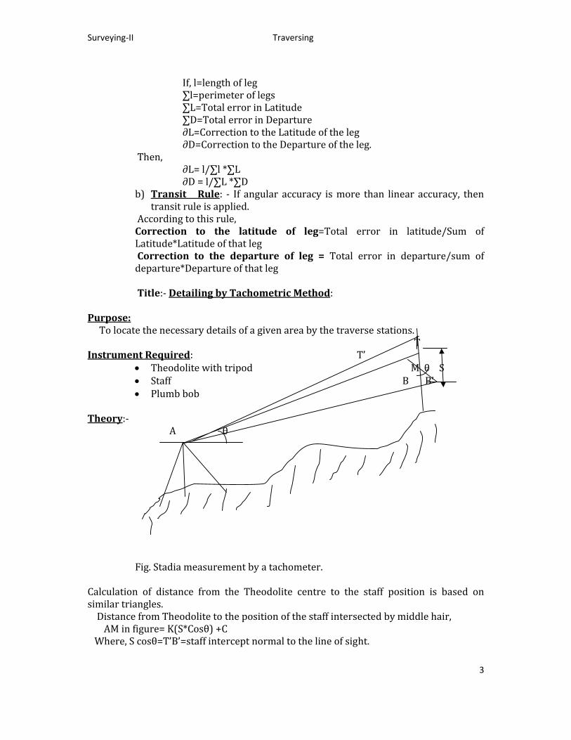
Surveying‐II Traversing
3
If, l=length of leg ∑l=perimeter of legs ∑L=Total error in Latitude ∑D=Total error in Departure ∂L=Correction to the Latitude of the leg ∂D=Correction to the Departure of the leg. Then, ∂L= l/∑l *∑L ∂D = l/∑L *∑D b) Transit Rule: ‐ If angular accuracy is more than linear accuracy, then
transit rule is applied. According to this rule, Correction to the latitude of leg=Total error in latitude/Sum of Latitude*Latitude of that leg Correction to the departure of leg = Total error in departure/sum of departure*Departure of that leg Title:‐ Detailing by Tachometric Method:
Purpose: To locate the necessary details of a given area by the traverse stations. T Instrument Required: T’
• Theodolite with tripod M θ S • Staff B B’ • Plumb bob
Theory:‐ A θ
Fig. Stadia measurement by a tachometer.
Calculation of distance from the Theodolite centre to the staff position is based on similar triangles. Distance from Theodolite to the position of the staff intersected by middle hair, AM in figure= K(S*Cosθ) +C Where, S cosθ=T’B’=staff intercept normal to the line of sight.
Surveying‐II Traversing
4
K=multiplying factor of theodolite which depends upon the focal length and length between top and bottom hair in the lens. C= additive constant= f+d Where, f= focal length D= distance from objective lens to centre of theodolite For horizontal sight, Horizontal distance between theodolite centre and staff station is, H=KS+C (where k=100 &C=0) generally For inclined line of sight, H=KS* Cos2θ. Where, θ= angle with horizontal S= staff intercept For vertical distance, from centre of theodolite to the middle hair position in staff. V=KS Cosθ*Sinθ= (KS Sin2θ)/2 If horizontal angle is taken, H=KS Sin2θ and V=1/2*KS Sin2θ Field Procedure:
1. Zero angles are set at the back sight to the traverse station. 2. Staff reading is taken i.e., bottom, middle and top at the necessary
position. 3. Staff man is allowed to go to the next position. 4. Vertical and horizontal angles are taken. 5. Height of instrument should be taken initially.
Now, the horizontal and vertical distances are obtained using formulas. Then by use of horizontal angles and distance we can plot the necessary details. The vertical distance is reduced to calculate the RL of staff stations which will serve for rough contouring in the topographic map.

Surveying‐II Traversing
5

45
Compound Curve:
IP (1+200m)
∆ 30˚30’40’’
TL D
(1+152.23 M) S (1+244.71 m)
N Φ E SC CS F
(1+122.23m) T1 G T2 (1+274.71m)
(TS) (ST)
A R R
Φ ∆‐2Φ Φ
∆
C
Fig. Compound curve with (Transition, Spiral and Circular curves)

46
6.4. Transition Curves:
A non‐ circular curve introduced between a straight and a circular curve is known as a transition curve. The curvature of transition curve varies from zero at its beginning to a definite value at it’s junction with the circular curve. The transition curve has the following advantages:
It enables to introduce super‐elevation in proportion to the rate of change of curvature. It avoids the danger of derailment at the point of commencement if full amount of super‐elevation is suddenly applied at the point.
It avoids over turning and side slipping of the moving vehicles. It eliminates discomforts caused to the passengers while negotiating a curve. Various types of transition curves are:
I. Cubical Spiral II. Cubic Parabola III. The Lemniscate curve
Cubical spiral and cubic parabolic transition curves are best suited to railway curves and Lemniscate
curves fro highway curves.
I. Cubical Spiral: The standard equation of a cubical spiral curve is given by
x =
Where, L = Total length of the transition curve T1 R = radius of the circular curve l x l =distance measured along the curve L x = perpendicular offset from the tangent Fig. Cubic spiral
II. Cubic Parabola : The standard equation of a cubic parabola is given by :
X=
y x where, y = distance measured along the tangent Fig. Cubic Parabola
III. The Lemniscate curve: The equation of this type of curve is given by:
r =
45˚ ρ
Where, r = radius of the curvature <α ρ = Polar ray of any point. Fig. The Lemniscate Curve α= Polar deflection angle i.e. angle between the polar ray and the straight.
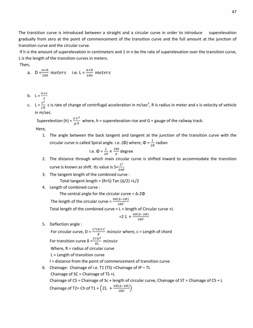
47
The transition curve is introduced between a straight and a circular curve in order to introduce superelevation gradually from zero at the point of commencement of the transition curve and the full amount at the junction of transition curve and the circular curve. If h is the amount of superelevation in centimeters and 1 in n be the rate of superelevation over the transition curve, L is the length of the transition curves in meters. Then,
a. D = i.e. L =
b. L =
c. L = c is rate of change of centrifugal acceleration in m/sec3, R is radius in meter and v is velocity of vehicle
in m/sec.
Superelevtion (h) = where, h = superelevation rise and G = gauge of the railway track.
Here, 1. The angle between the back tangent and tangent at the junction of the transition curve with the
circular curve is called Spiral angle. i.e. (Φ) where, Φ = radian
I.e. Φ = degree
2. The distance through which main circular curve is shifted inward to accommodate the transition
curve is known as shift. Its value is S=
3. The tangent length of the combined curve : Total tangent length = (R+S) Tan (∆/2) +L/2
4. Length of combined curve : The central angle for the circular curve = ∆‐2Φ
The length of the circular curve = ∆
˚
Total length of the combined curve = L + length of Circular curve +L
=2 ∆
˚
5. Deflection angle :
For circular curve, D = . where, c = Length of chord
For transition curve δ =
Where, R = radius of circular curve L = Length of transition curve l = distance from the point of commencement of transition curve.
6. Chainage: Chainage of i.e. T1 (TS) =Chainage of IP – TL Chainage of SC = Chainage of TS +L Chainage of CS = Chainage of Sc + length of circular curve, Chainage of ST = Chainage of CS + L
Chainage of T2= Ch of T1 + 2L ∆˚
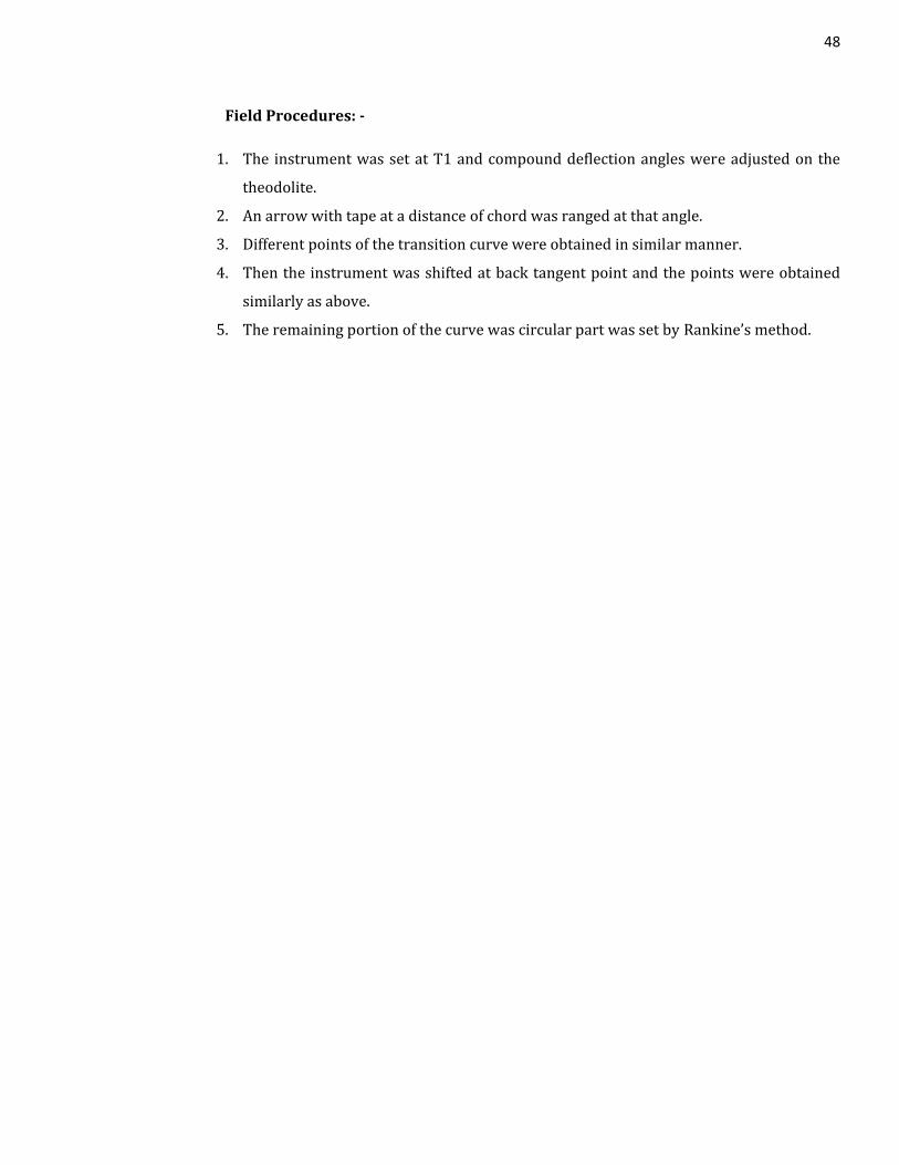
48
Field Procedures:
1. The instrument was set at T1 and compound deflection angles were adjusted on the
theodolite.
2. An arrow with tape at a distance of chord was ranged at that angle.
3. Different points of the transition curve were obtained in similar manner.
4. Then the instrument was shifted at back tangent point and the points were obtained
similarly as above.
5. The remaining portion of the curve was circular part was set by Rankine’s method.
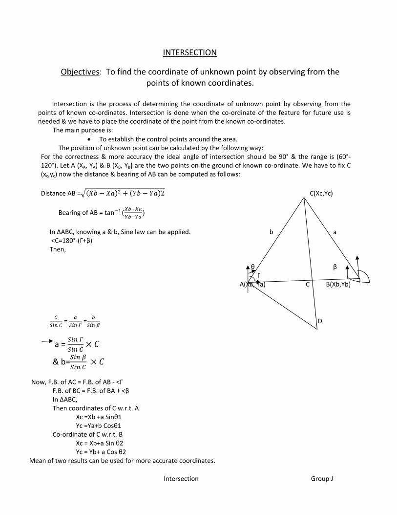
Intersection Group J
INTERSECTION
Objectives: To find the coordinate of unknown point by observing from the points of known coordinates.
Intersection is the process of determining the coordinate of unknown point by observing from the
points of known co‐ordinates. Intersection is done when the co‐ordinate of the feature for future use is needed & we have to place the coordinate of the point from the known co‐ordinates.
The main purpose is: • To establish the control points around the area.
The position of unknown point can be calculated by the following way: For the correctness & more accuracy the ideal angle of intersection should be 90° & the range is (60°‐
120°). Let A (XA, YA) & B (XB, YB) are the two points on the ground of known co‐ordinate. We have to fix C (xc,yc) now the distance & bearing of AB can be computed as follows:
Distance AB = 2 C(Xc,Yc)
Bearing of AB = tan
In ∆ABC, knowing a & b, Sine law can be applied. b a <C=180°‐(Γ+β) Then, θ β Γ A(Xa, Ya) C B(Xb,Yb)
=
=
D
a =
& b=
Now, F.B. of AC = F.B. of AB ‐ <Γ F.B. of BC = F.B. of BA + <β In ∆ABC, Then coordinates of C w.r.t. A Xc =Xb +a Sinθ1 Yc =Ya+b Cosθ1 Co‐ordinate of C w.r.t. B Xc = Xb+a Sin θ2 Yc = Yb+ a Cos θ2 Mean of two results can be used for more accurate coordinates.

Intersection Group J

INTERSECTION OF WATER TANK TOP AT NEATC, KHARIPATI, BHAKTAPUR
Group J
Now, the coordinates i.e. (E, N, R.L.) Of stations are as follows:
CP1 (1000, 1000, 1336.304) Cp2 (1031.497, 1039.595, 1336.606) W3 (1050.270, 1086.099, 1336.818)
Length of CP1CP2 =√∆ ∆ m
= 1031.497 1000 1039.595 1000 = 50.5947 m
Bearing of CP1CP2 = tan ∆∆
=tan ..
=N38˚30’5.47’’E
= 38˚30’5.47’’ (w.c.b.) Length of CP2W3 =√∆ ∆ m = 1050.270 1031.497 1086.099 1039.595 = 50.1502 m
Bearing of CP2W3 =tan ∆∆
W3
= tan ..
116˚19’35’’ <α
=N21˚58’59.61’’E W.T.T. = 21˚58’59.61’’ (W.C.B.) 30˚17’20.86’’ <β 166˚13’45’’ CP2
8˚30’50’’
CP1
Fig. intersection of water tank top
i.e. <CP2CP1W.T. =8˚30’50’’ <CP1CP2W.T. = (360˚‐193˚46’15’’) =166˚13’45’’
<CP2W3W.T. = (360˚‐243˚40’25’’) =116˚19’35’’
Now, From ∆CP1CP2W.T, <CP1+<CP2+<β =180˚ i.e. 8˚30’50’’+166˚13’45˚+<β =180˚ i.e. <β =5˚15’25’’ Now, Length of CP1CP2 = 50.5947 m From ∆CP1CP2W.T,
˚ ’ ’’
= . .
˚ = . .
˚
i.e.
.˚ ’ ’’
= . .
˚= . .
˚ ,
i.e. CP2W.T. =81.754 m
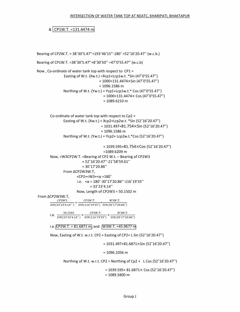
INTERSECTION OF WATER TANK TOP AT NEATC, KHARIPATI, BHAKTAPUR
Group J
& CP1W.T. =131.4474 m
Bearing of CP2W.T. = 38˚30’5.47’’+193˚46’15’’‐180˚ =52˚16’20.47’’ (w.c.b.)
Bearing of CP1W.T. =38˚30’5.47’’+8˚30’50’’ =47˚0’55.47’’ (w.c.b)
Now , Co‐ordinate of water tank top with respect to CP1 = Easting of W.t. (Xw.t.) =Xcp1+Lcp1w.t. *Sin (47˚0’55.47’’) = 1000+131.4474 Sin (47˚0’55.47’’) = 1096.1586 m Northing of W.t. (Yw.t.) = Ycp1+Lcp1w.t.* Cos (47˚0’55.47’’) = 1000+131.4474 Cos (47˚0’55.47’’) = 1089.6210 m Co‐ordinate of water tank top with respect to Cp2 = Easting of W.t. (Xw.t.) = Xcp2+Lcp2w.t. *Sin (52˚16’20.47’’) = 1031.497+81.754 Sin (52˚16’20.47’’) = 1096.1586 m Northing of W.t. (Yw.t.) = Ycp2+ Lcp2w.t.*Cos (52˚16’20.47’’) = 1039.595+81.754 Cos (52˚16’20.47’’) =1089.6209 m Now, <W3CP2W.T. =Bearing of CP2 W.t. – Bearing of CP2W3 = 52˚16’20.47’’‐21˚58’59.61’’ = 30˚17’20.86’’ From ∆CP2W3W.T, <CP2+<W3+<α =180˚ i.e. <α = 180˚‐30˚17’20.86’’‐116˚19’35’’ = 33˚23’4.14’’ Now, Length of CP2W3 = 50.1502 m From ∆CP2W3W.T,
˚ ’ . ’’ ’
= . .
˚ ’ ’’=
. .˚ ’ . ’’
i.e.
.˚ ’ . ’’
= . .
˚ ’ ’’ = . .
˚ ’ . ’’
i.e. CP2W.T. = 81.6871 m, and W3W.T. =45.9677 m
Now, Easting of W.t. w.r.t. CP2 = Easting of CP2+ L Sin (52˚16’20.47’’)
= 1031.497+81.6871 Sin (52˚16’20.47’’)
= 1096.1056 m
Northing of W.t. w.r.t. CP2 = Northing of Cp2 + L Cos (52˚16’20.47’’)
= 1039.595+ 81.6871 Cos (52˚16’20.47’’) = 1089.5800 m

INTERSECTION OF WATER TANK TOP AT NEATC, KHARIPATI, BHAKTAPUR
Group J
Now, Bearing of W3W.t. = 21˚58’59.61’’+243˚40’25’’‐180˚ =85˚39’24.61’’ (w.c.b.) Easting of W.t. w.r.t. W3 = Easting of W3+LSin (85˚39’24.61’’) = 1050.270 +45.9677 Sin (85˚39’24.61’’) = 1096.1057 m Northing of W.t. w.r.t. W3 = Northing of W3+ L Cos (85˚39’24.61’’) = 1086.099+45.9677 Cos (85˚39’24.61’’) = 1089.5801 m
FOR ALTITUDE CALCULATION:
Vertical angle from CP1 i.e.α1 = 11˚30’20’’ Now, Elevation difference between instrument station Cp1 and Water tank top i.e. H1 =D Tanα1 (D= Cp1W.T.) = 131.4474 Tan (11˚30’20’’) = 26.7565 m H.I. of CP1 = 1.44 m R.L. of W.t. w.r.t. Cp1 = R.L. of CP1+1.44+H1 =1336.304+1.44+26.7565 = 1364.500 m And, vertical angle from CP2 i.e. α2 = 17˚54’10’’ H2 = D Tan α2 (D= Cp2W.t.) = 81.754 Tan (17˚54’10’’) = 26.4101m H.I. of CP2 = 1.51 m R.L. of W.t. w.r.t. CP2 = R.L. of CP2 +1.51+ H2 = 1336.606+1.51+26.4101 = 1364.526 m And, Vertical Angle from W3 i.e. α3= 29˚41’55’’ H3= D Tan α3 (D= W3W.t.) = 45.9677 Tan (29˚41’55’’) = 26.2180 m H.I. of W3 = 1.48 m R.L. of W.t. w.r.t. W3 = R.L. of W3+1.48+ H3 = 1336.818 +1.48+26.2180 = 1364.516 m Now the Exact R.L. of W.t. = Average of R.L. from three station observation
= . . .
= 1364.514 m
Result: Hence the co‐ordinate of water tank top at NEATC is found as follows: S.N. Easting(m) Northing(m) Mean
Easting (m) Mean
Northing (m) Reduced Level (m)
Mean Reduced level (m)
Remarks
1 1096.1586 1089.6210 1096.1409m
1089.6073m
1364.500 1364.514m
Obs. from CP1
2 1096.1586 1089.6209 1364.526 Obs. from Cp2
3 1096.1057 1089.5801 1364.516 Obs. from W3

INTERSECTION OF WATER TANK TOP AT NEATC, KHARIPATI, BHAKTAPUR
Group J
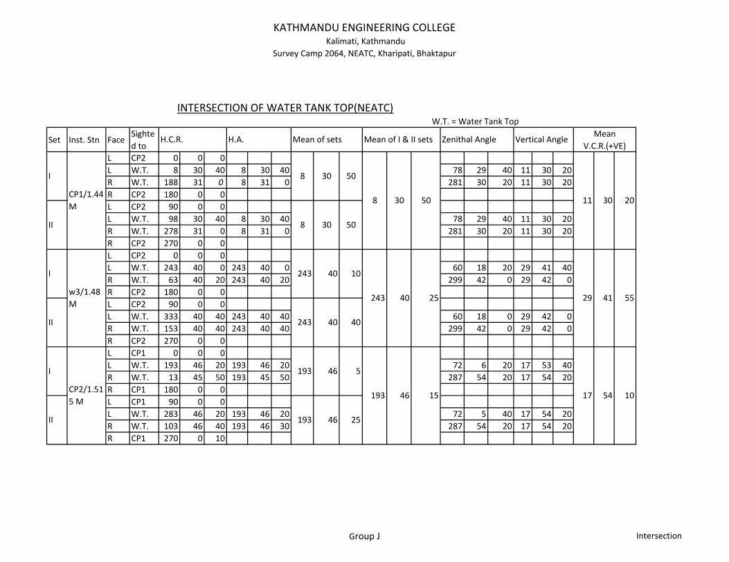
KATHMANDU ENGINEERING COLLEGE Kalimati, Kathmandu
Survey Camp 2064, NEATC, Kharipati, Bhaktapur
W.T. = Water Tank Top
Set Inst. Stn FaceSighted to
L CP2 0 0 0L W.T. 8 30 40 8 30 40 78 29 40 11 30 20R W.T. 188 31 0 8 31 0 281 30 20 11 30 20R CP2 180 0 0L CP2 90 0 0L W.T. 98 30 40 8 30 40 78 29 40 11 30 20R W.T. 278 31 0 8 31 0 281 30 20 11 30 20R CP2 270 0 0L CP2 0 0 0L W.T. 243 40 0 243 40 0 60 18 20 29 41 40R W.T. 63 40 20 243 40 20 299 42 0 29 42 0R CP2 180 0 0L CP2 90 0 0L W.T. 333 40 40 243 40 40 60 18 0 29 42 0R W.T. 153 40 40 243 40 40 299 42 0 29 42 0R CP2 270 0 0L CP1 0 0 0L W.T. 193 46 20 193 46 20 72 6 20 17 53 40R W.T. 13 45 50 193 45 50 287 54 20 17 54 20R CP1 180 0 0L CP1 90 0 0L W.T. 283 46 20 193 46 20 72 5 40 17 54 20R W.T. 103 46 40 193 46 30 287 54 20 17 54 20R CP1 270 0 10
54 10193 46 15 17
30 20
29 41 55
193 46 5
193 46 25
243 40 40
243 40
243
25
30 50
8 30 50
40 10I
II
w3/1.48 M
I
CP2/1.515 M
II
Vertical AngleMean
V.C.R.(+VE)
INTERSECTION OF WATER TANK TOP(NEATC)
I
CP1/1.44M
II
8 30 50
8
H.C.R. H.A. Mean of sets Mean of I & II sets Zenithal Angle
11
Group J Intersection
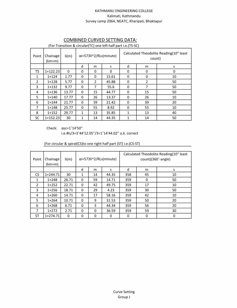
KATHMANU ENGINEERING COLLEGEKalimati, Kathmandu
Survey camp 2064, NEATC, Kharipati, Bhaktapur
Point Chainage(km+m)
li(m)
d m s d m sTS 1+122.23 0 0 0 0 0 0 01 1+124 1.77 0 0 15.61 0 0 102 1+128 5.77 0 2 45.88 0 2 503 1+132 9.77 0 7 55.6 0 7 504 1+136 13.77 0 15 44.77 0 15 505 1+140 17.77 0 26 13.37 0 26 106 1+144 21.77 0 39 21.42 0 39 207 1+148 25.77 0 55 8.92 0 55 108 1+152 29.77 1 13 35.85 1 13 40SC 1+152.23 30 1 14 44.35 1 14 50
Check: αsc=1˚14'50''i.e.Фs/3=3˚44'12.05''/3=1˚14'44.02'' o.k. correct
Point Chainage(km+m)
li(m)
d m s d m sCS 1+244.71 30 1 14 44.35 358 45 101 1+248 26.71 0 59 14.71 359 0 502 1+252 22.71 0 42 49.75 359 17 103 1+256 18.71 0 29 4.23 359 30 504 1+260 14.71 0 17 58.16 359 42 105 1+264 10.71 0 9 31.53 359 50 206 1+268 6.71 0 3 44.34 359 56 207 1+272 2.71 0 0 36.59 359 59 30ST 1+274.71 0 0 0 0 0 0 0
αi=573li^2/RLs(minute)Calculated Theodolite Reading(10" least
count)(360˚‐angle)
(For Transition & circular(TC) one left half part i.e.(TS‐SC)
(For circular & spiral(CS)to one right half part (ST) i.e.(CS‐ST)
COMBINED CURVED SETTING DATA:
αi=573li^2/RLs(minute)Calculated Theodolite Reading(10" least
count)
Curve SettingGroup J

45
Compound Curve:
IP (1+200m)
∆ 30˚30’40’’
TL D
(1+152.23 M) S (1+244.71 m)
N Φ E SC CS F
(1+122.23m) T1 G T2 (1+274.71m)
(TS) (ST)
A R R
Φ ∆‐2Φ Φ
∆
C
Fig. Compound curve with (Transition, Spiral and Circular curves)
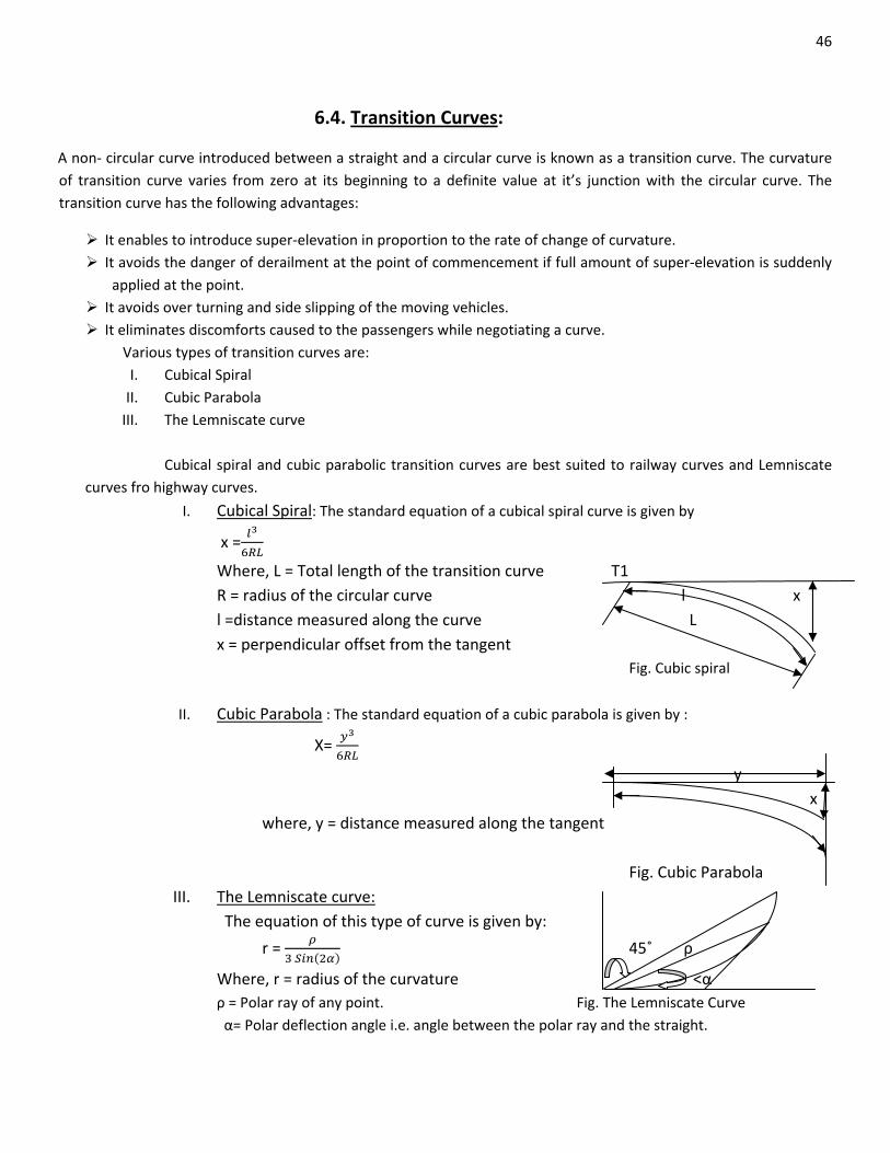
46
6.4. Transition Curves:
A non‐ circular curve introduced between a straight and a circular curve is known as a transition curve. The curvature of transition curve varies from zero at its beginning to a definite value at it’s junction with the circular curve. The transition curve has the following advantages:
It enables to introduce super‐elevation in proportion to the rate of change of curvature. It avoids the danger of derailment at the point of commencement if full amount of super‐elevation is suddenly applied at the point.
It avoids over turning and side slipping of the moving vehicles. It eliminates discomforts caused to the passengers while negotiating a curve. Various types of transition curves are:
I. Cubical Spiral II. Cubic Parabola III. The Lemniscate curve
Cubical spiral and cubic parabolic transition curves are best suited to railway curves and Lemniscate
curves fro highway curves.
I. Cubical Spiral: The standard equation of a cubical spiral curve is given by
x =
Where, L = Total length of the transition curve T1 R = radius of the circular curve l x l =distance measured along the curve L x = perpendicular offset from the tangent Fig. Cubic spiral
II. Cubic Parabola : The standard equation of a cubic parabola is given by :
X=
y x where, y = distance measured along the tangent Fig. Cubic Parabola
III. The Lemniscate curve: The equation of this type of curve is given by:
r =
45˚ ρ
Where, r = radius of the curvature <α ρ = Polar ray of any point. Fig. The Lemniscate Curve α= Polar deflection angle i.e. angle between the polar ray and the straight.

47
The transition curve is introduced between a straight and a circular curve in order to introduce superelevation gradually from zero at the point of commencement of the transition curve and the full amount at the junction of transition curve and the circular curve. If h is the amount of superelevation in centimeters and 1 in n be the rate of superelevation over the transition curve, L is the length of the transition curves in meters. Then,
a. D = i.e. L =
b. L =
c. L = c is rate of change of centrifugal acceleration in m/sec3, R is radius in meter and v is velocity of vehicle
in m/sec.
Superelevtion (h) = where, h = superelevation rise and G = gauge of the railway track.
Here, 1. The angle between the back tangent and tangent at the junction of the transition curve with the
circular curve is called Spiral angle. i.e. (Φ) where, Φ = radian
I.e. Φ = degree
2. The distance through which main circular curve is shifted inward to accommodate the transition
curve is known as shift. Its value is S=
3. The tangent length of the combined curve : Total tangent length = (R+S) Tan (∆/2) +L/2
4. Length of combined curve : The central angle for the circular curve = ∆‐2Φ
The length of the circular curve = ∆
˚
Total length of the combined curve = L + length of Circular curve +L
=2 ∆
˚
5. Deflection angle :
For circular curve, D = . where, c = Length of chord
For transition curve δ =
Where, R = radius of circular curve L = Length of transition curve l = distance from the point of commencement of transition curve.
6. Chainage: Chainage of i.e. T1 (TS) =Chainage of IP – TL Chainage of SC = Chainage of TS +L Chainage of CS = Chainage of Sc + length of circular curve, Chainage of ST = Chainage of CS + L
Chainage of T2= Ch of T1 + 2L ∆˚

48
Field Procedures:
1. The instrument was set at T1 and compound deflection angles were adjusted on the
theodolite.
2. An arrow with tape at a distance of chord was ranged at that angle.
3. Different points of the transition curve were obtained in similar manner.
4. Then the instrument was shifted at back tangent point and the points were obtained
similarly as above.
5. The remaining portion of the curve was circular part was set by Rankine’s method.
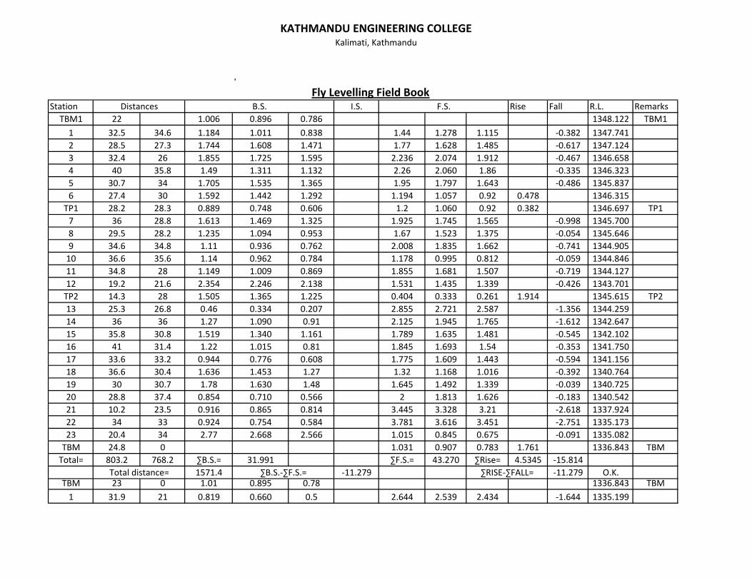
KATHMANDU ENGINEERING COLLEGEKalimati, Kathmandu
l
Station I.S. Rise Fall R.L. RemarksTBM1 22 1.006 0.896 0.786 1348.122 TBM1
1 32.5 34.6 1.184 1.011 0.838 1.44 1.278 1.115 ‐0.382 1347.7412 28.5 27.3 1.744 1.608 1.471 1.77 1.628 1.485 ‐0.617 1347.1243 32.4 26 1.855 1.725 1.595 2.236 2.074 1.912 ‐0.467 1346.6584 40 35.8 1.49 1.311 1.132 2.26 2.060 1.86 ‐0.335 1346.3235 30.7 34 1.705 1.535 1.365 1.95 1.797 1.643 ‐0.486 1345.8376 27.4 30 1.592 1.442 1.292 1.194 1.057 0.92 0.478 1346.315TP1 28.2 28.3 0.889 0.748 0.606 1.2 1.060 0.92 0.382 1346.697 TP17 36 28.8 1.613 1.469 1.325 1.925 1.745 1.565 ‐0.998 1345.7008 29.5 28.2 1.235 1.094 0.953 1.67 1.523 1.375 ‐0.054 1345.6469 34.6 34.8 1.11 0.936 0.762 2.008 1.835 1.662 ‐0.741 1344.90510 36.6 35.6 1.14 0.962 0.784 1.178 0.995 0.812 ‐0.059 1344.84611 34.8 28 1.149 1.009 0.869 1.855 1.681 1.507 ‐0.719 1344.12712 19.2 21.6 2.354 2.246 2.138 1.531 1.435 1.339 ‐0.426 1343.701TP2 14.3 28 1.505 1.365 1.225 0.404 0.333 0.261 1.914 1345.615 TP213 25.3 26.8 0.46 0.334 0.207 2.855 2.721 2.587 ‐1.356 1344.25914 36 36 1.27 1.090 0.91 2.125 1.945 1.765 ‐1.612 1342.64715 35.8 30.8 1.519 1.340 1.161 1.789 1.635 1.481 ‐0.545 1342.10216 41 31.4 1.22 1.015 0.81 1.845 1.693 1.54 ‐0.353 1341.75017 33.6 33.2 0.944 0.776 0.608 1.775 1.609 1.443 ‐0.594 1341.15618 36.6 30.4 1.636 1.453 1.27 1.32 1.168 1.016 ‐0.392 1340.76419 30 30.7 1.78 1.630 1.48 1.645 1.492 1.339 ‐0.039 1340.72520 28.8 37.4 0.854 0.710 0.566 2 1.813 1.626 ‐0.183 1340.54221 10.2 23.5 0.916 0.865 0.814 3.445 3.328 3.21 ‐2.618 1337.92422 34 33 0.924 0.754 0.584 3.781 3.616 3.451 ‐2.751 1335.17323 20.4 34 2.77 2.668 2.566 1.015 0.845 0.675 ‐0.091 1335.082TBM 24.8 0 1.031 0.907 0.783 1.761 1336.843 TBMTotal= 803.2 768.2 ∑B.S.= 31.991 ∑F.S.= 43.270 ∑Rise= 4.5345 ‐15.814
1571.4 ‐11.279 ‐11.279 O.K.TBM 23 0 1.01 0.895 0.78 1336.843 TBM
1 31.9 21 0.819 0.660 0.5 2.644 2.539 2.434 ‐1.644 1335.199
Fly Levelling Field Book
Total distance= ∑B.S.‐∑F.S.= ∑RISE‐∑FALL=
Distances B.S. F.S.

KATHMANDU ENGINEERING COLLEGEKalimati, Kathmandu
2 17.8 30 2.446 2.357 2.268 1.078 0.927 0.775 ‐0.267 1334.9323 16 11 2.451 2.371 2.291 0.78 0.725 0.67 1.632 1336.5644 12 9.9 2.312 2.252 2.192 0.753 0.704 0.654 1.6675 1338.2325 19.3 5.7 2.222 2.126 2.029 0.71 0.682 0.653 1.5705 1339.8026 30.8 21.5 1.998 1.844 1.69 1.37 1.263 1.155 0.863 1340.6657 29.1 36 1.681 1.536 1.39 1.936 1.756 1.576 0.088 1340.7538 31.5 32.2 1.321 1.164 1.006 1.582 1.421 1.26 0.1145 1340.8689 25.8 39 1.545 1.413 1.28 0.91 0.715 0.52 0.4485 1341.31610 26.3 35.8 1.882 1.751 1.619 1.449 1.270 1.091 0.1425 1341.45911 26.8 25.8 1.686 1.552 1.418 1.301 1.172 1.043 0.5785 1342.03712 32.1 32.4 1.875 1.715 1.554 1.462 1.300 1.138 0.252 1342.28913 38.1 37.6 3.856 3.666 3.475 1.046 0.858 0.67 0.8565 1343.146TP2 12.3 31.4 0.387 0.326 0.264 1.341 1.184 1.027 2.4815 1345.627 TP214 19 30 1.568 1.473 1.378 2.365 2.215 2.065 ‐1.890 1343.73815 28 36 1.67 1.530 1.39 1.085 0.905 0.725 0.568 1344.30616 30 27.6 1.69 1.540 1.39 1.344 1.206 1.068 0.324 1344.6317 24.8 25.5 1.856 1.732 1.608 1.545 1.418 1.29 0.1225 1344.75218 25.5 27.2 1.922 1.795 1.667 1.384 1.248 1.112 0.484 1345.23619 29.6 27.6 1.41 1.262 1.114 1.268 1.130 0.992 0.6645 1345.90120 27.8 27.5 1.55 1.411 1.272 1.299 1.162 1.024 0.1005 1346.001TP1 30 14.4 1.185 1.035 0.885 0.78 0.708 0.636 0.703 1346.704 TP121 24.4 33.9 1.273 1.151 1.029 1.609 1.440 1.27 ‐0.405 1346.322 22.4 36 1.636 1.524 1.412 1.516 1.336 1.156 ‐0.185 1346.11523 30.2 29 2.001 1.850 1.699 1.645 1.500 1.355 0.024 1346.13924 24 29 1.504 1.384 1.264 1.14 0.995 0.85 0.855 1346.99425 29 34.4 1.62 1.475 1.33 1.294 1.122 0.95 0.262 1347.25626 26.7 28 1.457 1.324 1.19 1.353 1.213 1.073 0.262 1347.51827 20.2 21.2 1.578 1.472 1.366 1.371 1.270 1.169 0.0535 1347.571
TBM1 19.8 0 1.01 0.912 0.814 0.56 1348.131 TBM1Total 784.2 796.6 ∑B.S.= 47.581 ∑F.S.= 36.293 ∑Rise= 15.678 ‐4.39
total distance= 1580.811.288 ∑RISE‐∑FALL= 11.288 11.288
Error= 0.009 (9mm)Total Perimeter= 3152.2 m
∑B.S.‐∑F.S.= last R.L.‐First R.L.=

KATHMANDU ENGINEERING COLLEGEKalimati, Kathmandu
Permissible Error= 25√K mm 25√3.1522 K is in kilometer≈ 44.38609 mm
O.k. Within Precision
Station loop Loop
distanceR.L Error Correction
Corrected R.L.
Remarks
TBM1 1348.122TP1 TBM1‐TP1 1346.697TP1 1346.697 1346.692 TP1TBM1 TP1‐TBM1 1348.131 ‐0.0045
TP1 1346.697TP2 TP1‐TP2 1345.615TP2 1345.615 ‐0.0053 1345.610 TP2TP1 TP2‐TP1 1346.704
TP2 1345.615TBM TP2‐TBM 1336.843 ‐0.0086 1336.834 TBMTBM 1336.843TP2 TBM‐TP2 1345.627
940.7
1495.1 0.017
0.012
Correction For R.L.
0.009910.1
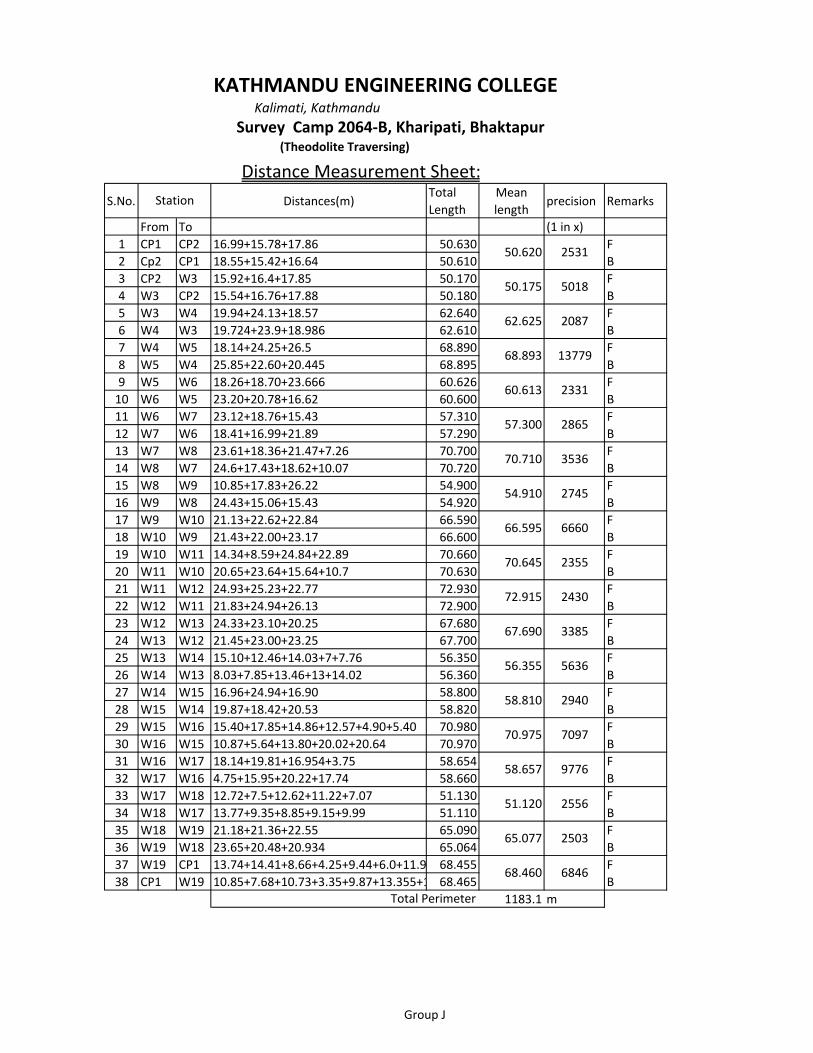
Kalimati, Kathmandu
S.No. Distances(m)Total Length
Mean length
precision Remarks
From To (1 in x)1 CP1 CP2 16.99+15.78+17.86 50.630 F2 Cp2 CP1 18.55+15.42+16.64 50.610 B3 CP2 W3 15.92+16.4+17.85 50.170 F4 W3 CP2 15.54+16.76+17.88 50.180 B5 W3 W4 19.94+24.13+18.57 62.640 F6 W4 W3 19.724+23.9+18.986 62.610 B7 W4 W5 18.14+24.25+26.5 68.890 F8 W5 W4 25.85+22.60+20.445 68.895 B9 W5 W6 18.26+18.70+23.666 60.626 F10 W6 W5 23.20+20.78+16.62 60.600 B11 W6 W7 23.12+18.76+15.43 57.310 F12 W7 W6 18.41+16.99+21.89 57.290 B13 W7 W8 23.61+18.36+21.47+7.26 70.700 F14 W8 W7 24.6+17.43+18.62+10.07 70.720 B15 W8 W9 10.85+17.83+26.22 54.900 F16 W9 W8 24.43+15.06+15.43 54.920 B17 W9 W10 21.13+22.62+22.84 66.590 F18 W10 W9 21.43+22.00+23.17 66.600 B19 W10 W11 14.34+8.59+24.84+22.89 70.660 F20 W11 W10 20.65+23.64+15.64+10.7 70.630 B21 W11 W12 24.93+25.23+22.77 72.930 F22 W12 W11 21.83+24.94+26.13 72.900 B23 W12 W13 24.33+23.10+20.25 67.680 F24 W13 W12 21.45+23.00+23.25 67.700 B25 W13 W14 15.10+12.46+14.03+7+7.76 56.350 F26 W14 W13 8.03+7.85+13.46+13+14.02 56.360 B27 W14 W15 16.96+24.94+16.90 58.800 F28 W15 W14 19.87+18.42+20.53 58.820 B29 W15 W16 15.40+17.85+14.86+12.57+4.90+5.40 70.980 F30 W16 W15 10.87+5.64+13.80+20.02+20.64 70.970 B31 W16 W17 18.14+19.81+16.954+3.75 58.654 F32 W17 W16 4.75+15.95+20.22+17.74 58.660 B33 W17 W18 12.72+7.5+12.62+11.22+7.07 51.130 F34 W18 W17 13.77+9.35+8.85+9.15+9.99 51.110 B35 W18 W19 21.18+21.36+22.55 65.090 F36 W19 W18 23.65+20.48+20.934 65.064 B37 W19 CP1 13.74+14.41+8.66+4.25+9.44+6.0+11.9 68.455 F38 CP1 W19 10.85+7.68+10.73+3.35+9.87+13.355+1 68.465 B
1183.1 m
2556
2503
6846
6660
2355
2430
3385
5636
65.077
68.460
2531
5018
2087
13779
2331
2865
3536
7097
2745
67.690
56.355
58.810
70.975
58.657
2940
9776
Station
51.120
57.300
70.710
54.910
66.595
70.645
72.915
KATHMANDU ENGINEERING COLLEGE
Survey Camp 2064‐B, Kharipati, Bhaktapur(Theodolite Traversing)
Total Perimeter
Distance Measurement Sheet:
50.620
50.175
62.625
68.893
60.613
Group J

Horizontal Angle Observation Sheet
Instrument At: W7Ht. of instrument axis : 1.455MSighted to
Face H.Dist.
d m s d m s d m s d m s d m s d m s T M Bw6 L 0 0 20W8 L 127 38 0 89 32 0 0 28 0 1.44 1.085 0.73 70.995W8 R 307 39 0 270 28 20 0 28 20 1.25 0.895 0.54 71.000W6 R 180 1 40W6 L 90 0 0W8 L 217 38 0W8 R 7 38 0W6 R 240 0 40
Instrument At: W8Ht. of instrument axis : 1.454MSighted to Face Staff Reading H.Dist.
d m s d m s d m s d m s d m s d m s T M BW7 L 0 0 0W9 L 197 29 40 87 40 0 2 20 0 1.2 0.923 0.65 55.408W9 R 17 29 40 272 20 20 2 20 20 1.09 0.815 0.54 55.000W7 R 180 0 20W7 L 90 0 20W9 L 287 29 20W9 R 107 30 0W7 R 270 0 20
H.C.R. H.A. Mean H.A. V.C.R. V. Angle
V. Angle
Mean V. Angle
37 20
127 37 30
0
V.C.R. Staff Reading
KATHMANDU ENGINEERING COLLEGEKalimati, Kathmandu
THEODOLITE FIELD OBSERVATION SHEET(THEODOLITE TRAVERSING)
(SURVEY Camp 2064‐B, Kharipati, Bhaktapur)
H.C.R. H.A. Mean H.A.
20
127 37 40
127
Mean V. Angle
37 2028 10
127 37 40
127
197 29 20
197 29 20
197 29 0
197 29 40
197 29
2 20 10
Group j
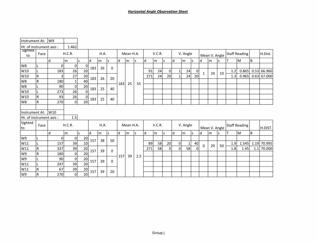
Horizontal Angle Observation Sheet
Instrument At: W9
Ht. of instrument axis : 1.462Sighted
to Face Staff Reading H.Dist.
d m s d m s d m s d m s d m s d m s T M BW8 L 0 0 0W10 L 183 26 20 91 24 0 1 24 0 1.2 0.865 0.53 66.960W10 R 3 27 20 271 24 20 1 24 20 1.3 0.965 0.63 67.000W8 R 180 1 40W8 L 90 0 20W10 L 273 26 0W10 R 93 26 0W8 R 270 0 20
Instrument At: W10Ht. of instrument axis : 1.5Sighted to
Face Staff ReadingH.DIST.
d m s d m s d m s d m s d m s d m s T M BW9 L 0 0 20W11 L 157 39 10 89 58 20 0 1 40 1.9 1.545 1.19 70.995W11 R 337 39 20 271 58 0 0 58 0 1.8 1.45 1.1 70.000W9 R 180 0 20W9 L 90 0 20W11 L 247 39 20W11 R 67 39 20W9 R 270 0 20
157 39 20
39 0
183 26 0
183 26 20
183 25
183
157 39 0
157
40
V. AngleH.C.R. H.A. Mean H.A. V.C.R.
40
10
Mean V. Angle
Mean V. Angle
24
H.C.R. H.A. Mean H.A. V.C.R. V. Angle
1
183 552525
290 50
157 39 2.5
157 38 50
Group j

Horizontal Angle Observation Sheet
Instrument At: W11Ht. of instrument axis : 1.43Sighted to
Face Staff ReadingH.Dist.
d m s d m s d m s d m s d m s d m s T BW10 L 0 0 20W12 L 117 38 20 117 38 0 95 51 0 5 51 0 1.2 0.83 0.46 73.231W12 R 297 38 0 264 9 0 5 51 0 1.2 0.833 0.47 72.736W10 R 180 0 0 117 38 0W10 L 90 0 20W12 L 207 38 0 117 37 40W12 R 27 38 20W10 R 270 0 20 117 38 0
Instrument At: W12Ht. of instrument axis : 1.455Sighted to
Face Staff ReadingH.DIST.
d m s d m s d m s d m s d m s d m s T M BW11 L 0 0 20 0W13 L 158 58 20 158 58 0 93 36 20 3 36 20 1.2 0.863 0.53 67.500W13 R 338 58 40 266 19 50 3 40 0 3.12 2.78 2.44 67.727W11 R 180 0 20 158 58 20W11 L 90 0 20W13 L 248 58 40 158 58 20W13 R 68 58 40W11 R 270 0 0 158 58 40
158 58 20
3 38 10
H.C.R. H.A. Mean H.A.
H.C.R. H.A. Mean H.A.
51 0
117 37 55
V.C.R. V. Angle
5
Mean V. Angle
V.C.R. V. AngleMean V. Angle
Group j

Horizontal Angle Observation Sheet
Instrument At: W13Ht. of instrument axis : 1.38Sighted Face Staff Reading H.DIST.
d m s d m s d m s d m s d m s d m s T M BW12 L 0 0 20W14 L 204 56 50 204 56 30 89 20 10 0 39 50 0.9 0.618 0.34 56.500W14 R 24 57 20 270 39 50 0 39 50 1.1 0.818 0.54 56.494W12 R 180 0 40 204 56 40W12 L 90 0 20W14 L 294 56 20 204 56 0W14 R 114 56 40W12 R 270 0 20 204 56 20
Instrument At: W14Ht. of instrument axis : 1.39Sighted to Face Staff Reading H.DIST.
d m s d m s d m s d m s d m s d m s T M BW13 L 0 0 20W15 L 165 24 40 165 24 20 94 23 20 4 23 20 1.2 0.906 0.61 58.800W15 R 345 24 30 265 36 0 4 23 40 1.2 0.905 0.61 58.654W13 R 180 0 0 165 24 30W13 L 90 0 20W15 L 255 24 40 165 24 20W15 R 75 24 0W13 R 270 0 20 165 23 40
23 30
165 24 12.5
204 22.556
0 34 50
H.C.R. H.A. Mean H.A. V.C.R. V. Angle Mean V. Angle
H.C.R. H.A. Mean H.A. V.C.R. V. Angle Mean V. Angle
4
Group j

Horizontal Angle Observation Sheet
Instrument At: W15Ht. of instrument axis : 1.4Sighted to
Face Staff ReadingH.DIST.
d m s d m s d m s d m s d m s d m s T M BW14 L 0 0 20W16 L 178 40 40 178 40 30 268 37 0 1 23 0 1.2 0.845 0.49 71.000W16 R 358 38 20 91 22 40 1 22 40 1.3 0.945 0.59 70.959W14 R 179 57 40 178 40 40W14 L 90 0 20W16 L 268 45 0 178 44 40W16 R 88 45 40W14 R 270 2 40 178 43 0
Instrument At: W16Ht. of instrument axis : 1.31Sighted to
Face Staff ReadingH.DIST.
d m s d m s d m s d m s d m s d m s T M BW15 L 0 0 20W17 L 107 44 20 107 44 0 95 6 0 5 6 0 0.8 0.508 0.22 58.500W17 R 287 44 20 264 22 20 5 37 40 1 0.705 0.41 58.584W15 R 180 0 0 107 44 20W15 L 90 0 0W17 L 197 44 0 107 44 0W17 R 17 44 40W15 R 270 0 40 107 44 0
12.542
V. AngleMean V. Angle
107 44 10
5 21 50
1 22 50
V.C.R.
Mean V. AngleV. AngleV.C.R.Mean H.A.H.A.H.C.R.
Mean H.A.H.A.H.C.R.
178
Group j
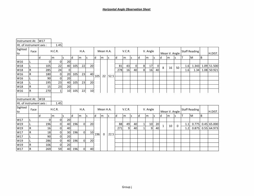
Horizontal Angle Observation Sheet
Instrument At: W17Ht. of instrument axis : 1.45Sighted to
Face Staff ReadingH.DIST.
d m s d m s d m s d m s d m s d m s T M BW16 L 0 0 20W18 L 105 22 40 105 22 20 81 43 0 8 17 0 1.6 1.343 1.09 51.500W18 R 285 24 0 278 16 40 8 16 40 1.6 1.34 1.08 50.921W16 R 180 0 20 105 23 40W16 L 90 0 20W18 L 195 23 40 105 23 20W18 R 15 23 20W16 R 270 1 10 105 22 10
Instrument At: W18Ht. of instrument axis : 1.45Sighted to
Face Staff ReadingH.DIST.
d m s d m s d m s d m s d m s d m s T M BW17 L 0 0 20W19 L 196 0 40 196 0 20 88 49 40 1 10 20 1.1 0.775 0.45 65.000W19 R 16 0 40 271 9 40 1 9 40 1.2 0.875 0.55 64.973W17 R 18 0 30 196 0 10W17 L 90 0 20W19 L 286 0 40 196 0 20W19 R 106 0 20W17 R 269 59 40 196 0 40
196 0 22.5
1 10 0
H.C.R. H.A. Mean H.A. V.C.R. V. AngleMean V. Angle
V. AngleMean V. Angle
105 22 52.5
8 16 50
H.C.R. H.A. Mean H.A. V.C.R.
Group j

Horizontal Angle Observation Sheet
Instrument At: W19Ht. of instrument axis : 1.4Sighted to
Face Staff ReadingH.DIST.
d m s d m s d m s d m s d m s d m s T M BW18 L 0 0 20CP1 L 158 49 0 158 48 40 81 24 50 8 35 10 1.69 1.343 1 68.500CP1 R 338 45 20 279 24 20 9 24 20 1.89 1.534 1.18 68.581W18 R 179 58 0 158 47 20W18 L 90 0 20CP1 L 248 44 10 158 43 50CP1 R 68 50 10W18 R 269 58 30 158 51 40
Instrument At: CP1Ht. of instrument axis : 1.54Sighted to
Face Staff ReadingH.DIST.
d m s d m s d m s d m s d m s d m s T M BW19 L 0 0 0CP2 L 206 1 0 206 1 0 90 18 30 0 18 30 1.24 0.987 0.73 50.600CP2 R 26 1 0 269 41 40 0 18 20 1.51 1.254 1 50.699W19 R 180 0 0 206 1 0W19 L 90 0 0CP2 L 296 1 20 206 1 20CP2 R 116 1 20W19 R 270 0 0 206 1 20
45
H.C.R. H.A. Mean H.A. V.C.R. V. AngleMean V. Angle
158 47 52.5
H.C.R. H.A. Mean H.A. V.C.R. V. AngleMean V. Angle
206 1 10
250 18
8 59
Group j

Horizontal Angle Observation Sheet
Instrument At: CP2Ht. of instrument axis : 1.5Sighted to
Face Staff ReadingH.DIST.
d m s d m s d m s d m s d m s d m s T M BCP1 L 0 0 20W3 L 163 29 40 163 29 30 81 52 20 8 7 40 1.32 1.064 0.81 50.300W3 R 343 29 40 278 7 30 8 7 30CP1 R 180 0 20 163 29 20CP1 L 90 0 20W3 L 253 29 40 163 29 20W3 R 73 29 20CP1 R 270 0 50 163 28 30
Instrument At: W3Ht. of instrument axis : 1.32Sighted to
Face Staff ReadingH.DIST.
d m s d m s d m s d m s d m s d m s T M BCP2 L 0 0 0W4 L 236 6 20 236 6 20 90 11 0 0 11 0 0.8 0.49 0.18 62.000W4 R 56 6 0 269 49 0 0 11 0CP2 R 180 0 0 236 6 0CP2 L 90 0 20W4 L 326 6 40 236 6 20W4 R 146 6 40CP2 R 270 1 0 236 6 40
236 6 5
V.C.R. V. AngleMean V. Angle
0 11 0
163 29 10
H.C.R. H.A. Mean H.A.
H.C.R. H.A. Mean H.A. V.C.R. V. AngleMean V. Angle
8 7 35
Group j

Horizontal Angle Observation Sheet
Instrument At: W4Ht. of instrument axis : 1.32Sighted to
Face Staff ReadingH.DIST.
d m s d m s d m s d m s d m s d m s T M BW5 L 0 0 20W3 L 117 9 40 117 9 20 90 6 50 0 6 50 1.4 1.05 0.71 69.000W3 R 297 8 40 269 53 0 0 7 0 1.5 1.05 0.81 69.000W5 R 180 0 0 117 8 40W5 L 90 0 20W3 L 207 9 40 117 9 20W3 R 27 9 40W5 R 270 0 20 117 9 20
Instrument At: W5Ht. of instrument axis : 1.42Sighted to
Face Staff ReadingH.DIST.
d m s d m s d m s d m s d m s d m s T M BW4 L 0 0 20W6 L 139 51 50 139 51 30 90 50 0 0 50 0 0.9 0.595 0.29 61.000W6 R 319 51 20 269 54 90 0 4 30 1 0.695 0.39 60.996W4 R 120 0 20 139 51 0W4 L 90 0 20W6 L 229 51 20 139 51 0W6 R 49 51 40W4 R 270 0 20 139 51 20
V. AngleMean V. Angle
117 9 10
H.C.R. H.A. Mean H.A. V.C.R.
V.C.R. V. AngleMean V. Angle
0 6 55
H.C.R. H.A. Mean H.A.
15
139 51 25
0 27
Group j
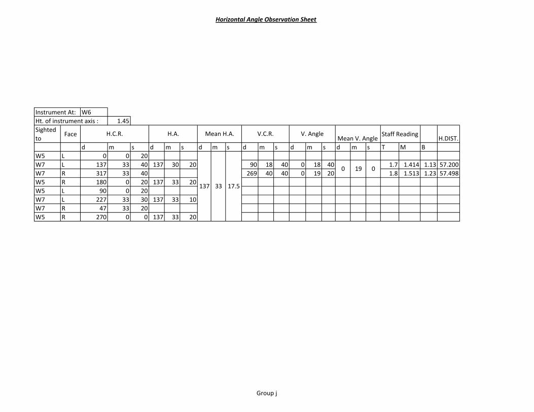
Horizontal Angle Observation Sheet
Instrument At: W6Ht. of instrument axis : 1.45Sighted to
Face Staff ReadingH.DIST.
d m s d m s d m s d m s d m s d m s T M BW5 L 0 0 20W7 L 137 33 40 137 30 20 90 18 40 0 18 40 1.7 1.414 1.13 57.200W7 R 317 33 40 269 40 40 0 19 20 1.8 1.513 1.23 57.498W5 R 180 0 20 137 33 20W5 L 90 0 20W7 L 227 33 30 137 33 10W7 R 47 33 20W5 R 270 0 0 137 33 20
H.C.R. H.A. Mean H.A. V.C.R. V. AngleMean V. Angle
137 33 17.5
0 19 0
Group j

Horizontal Angle Observation Sheet
Group j

Horizontal Angle Observation Sheet
Group j

Horizontal Angle Observation Sheet
Group j

Horizontal Angle Observation Sheet
Group j

Horizontal Angle Observation Sheet
Group j

Horizontal Angle Observation Sheet
Group j

Horizontal Angle Observation Sheet
Group j

Horizontal Angle Observation Sheet
Group j

Horizontal Angle Observation Sheet
Group j

Horizontal Angle Observation Sheet
Group j

Horizontal Angle Observation Sheet
Group j

Traverse Station
Corrections in second Remarks
d m s S d m sCP1 206 1 10 12 206 1 22CP2 163 29 10 11 163 29 21W3 236 6 5 12 236 6 17W4 117 9 10 11 117 9 21W5 139 51 25 11 139 51 36W6 137 33 17.5 11 137 33 28.5W7 127 37 30 11 127 37 41W8 197 29 20 12 197 29 32W9 183 25 55 12 183 26 7W10 157 39 2.5 11 157 39 13.5W11 117 37 55 11 117 38 6W12 158 58 20 11 158 58 31W13 204 56 22.5 12 204 56 34.5W14 165 24 12.5 11 165 24 23.5W15 178 42 12.5 11 178 42 23.5W16 107 44 10 11 107 44 21W17 105 22 52.5 11 105 23 3.5W18 196 0 22.5 12 196 0 34.5W19 158 47 52.5 11 158 48 3.5
SUM= 3059 56 25 215 3050 593 420Theoritical Sum= o.k.
sum= (2*19‐4)*90=3060 degreeError= 0°3'35''Precision=C√N(1√19)' =4'21.53'' O.K. within permissible error.
(2*n‐4)*90 3060°0'0''
Survey Camp 2064‐B, Kharipati, Bhaktapur(Theodolite Traversing)
KATHMANDU ENGINEERING COLLEGEKalimati, Kathmandu
Computation (angle Reduction Sheet)
Horizontal Angle Corrected Angles
Group J

R.L. Remarks
Easting Diff. Northing Diff. Easting Diff. Northing Diff. Easting Northing
CP1 (‐) (+) 1336.304 CP1CP2 61 51 35.7 38 30 5.74 1031.497 1039.595 1336.606 CP2J3 199 34 13.2 53.925 280 21 41.16 ‐53.047 9.699 ‐0.039 0.033 ‐53.008 9.732 978.489 1049.33 1335.794 J3J4 160 57 20.3 38.194 299 55 54.35 ‐33.104 19.058 ‐0.028 0.023 ‐33.076 19.081 945.417 1068.408 1333.182 J4J5 158 18 43.3 42.682 280 53 14.68 ‐41.914 8.062 ‐0.031 0.026 ‐41.883 8.088 903.532 1076.496 1328.614 J5J6 198 20 54.9 38.405 259 11 58.02 ‐37.723 ‐7.197 ‐0.028 0.023 ‐37.695 ‐7.173 865.834 1069.322 1326.843 J6
W12 57 57 50 52.146 277 32 52.93 ‐51.696 6.850 ‐0.038 0.032 ‐51.658 6.881 814.177 1076.203 1327.774 W12W13 155 30 42.93 1324.644 W13
sum= 225.352 ‐217.484 36.471 ‐0.164 0.137 ‐217.320 36.608Actual Easting Difference =
0.164‐0.137
0.214
Northing Diff.(l cosѲ)
Correction for Corrected Independent
KATHMANDU ENGINEERING COLLEGEKalimati, Kathmandu
(THEODOLITE TRAVERSING)
(SURVEY Camp 2064‐B, Kharipati, Bhaktapur)
Stn. H.Angle (adjusted) Distance(m) Bearing(Corrected)Easting
Diff.(l sinѲ)
COMPUTATION (GALE'S TABLE) Link Traverse
(814.177‐1031.497)= ‐217.32
Bearing of CP1‐CP2=tan^‐1(31.497/39.595) =38°30'5.47''(actual)Bearing of W12‐W13=tan^‐1(28.065/‐61.610)=155˚30'41.66''(actual)
Actual Northing Difference=(1076.203‐1039.595)=36.608Error in Easting= (217.484‐217.32)=Error in Northing= (36.471‐36.608)=
Closing error= Precision i.e. 1 in 1053.037 o.k.

KATHMANDU ENGINEERING COLLEGE (kalimati, Kathmandu)
Levelling Field BookStn. Distance(m) Rise Fall R.L. Correction Corrected R.L. Remarks
T M B T M B (+)TBM 26.8 1.656 1.522 1.388 1336.864 1336.864 TBM
W3 58.2 1.964 1.7795 1.595 1.675 1.569 1.462 ‐0.047 1336.818 0.001 1336.818 W3W4 61.4 1.717 1.5385 1.36 1.249 1.121 0.992 0.659 1337.477 0.002 1337.478 W4
W5 63.9 1.926 1.7735 1.621 1.56 1.393 1.226 0.146 1337.622 0.002 1337.624 W5
W6 67.4 1.595 1.4095 1.224 1.185 1.034 0.882 0.740 1338.362 0.003 1338.365 W6W7 49.3 1.526 1.3835 1.241 1.798 1.694 1.59 ‐0.285 1338.078 0.004 1338.081 W71 50.5 2.519 2.4745 2.43 1.115 0.907 0.699 0.477 1338.554 0.004 1338.558W8 21.1 0.493 0.4405 0.388 2.044 1.991 1.938 0.484 1339.038 0.004 1339.042 W8
W9 66.9 0.533 0.4285 0.324 4.055 3.825 3.595 ‐3.385 1335.653 0.005 1335.658 W9W10 73.9 3.205 3.066 2.927 1.692 1.462 1.231 ‐1.033 1334.620 0.006 1334.626 W10W11 49.5 1.056 1.0285 1.001 3.25 3.030 2.81 0.036 1334.656 0.006 1334.662 W11
2 44.9 0.417 0.352 0.287 4.745 4.586 4.426 ‐3.557 1331.099 0.007 1331.106
W12 45.5 0.334 0.2565 0.179 3.834 3.684 3.534 ‐3.332 1327.767 0.007 1327.774 W12
W13 101.3 2.743 2.499 2.255 3.65 3.388 3.125 ‐3.131 1324.636 0.008 1324.644 W13
W14 45.1 0.69 0.5405 0.391 1.137 1.061 0.985 1.438 1326.074 0.009 1326.083 W14
W15 67.2 0.995 0.8525 0.71 4.75 4.557 4.363 ‐4.016 1322.058 0.010 1322.068 W15
W16 83.2 0.852 0.656 0.46 2.205 1.985 1.765 ‐1.133 1320.926 0.010 1320.936 W163 16.1 0.764 0.7 0.636 3.785 3.769 3.752 ‐3.113 1317.813 0.011 1317.824
W17 33.4 3.657 3.5565 3.456 2.112 2.046 1.979 ‐1.346 1316.468 0.011 1316.479 W17
4 14.1 3.85 3.808 3.766 0.59 0.562 0.533 2.995 1319.463 0.011 1319.4745 14.9 2.569 2.508 2.447 0.36 0.347 0.333 3.462 1322.924 0.011 1322.935
W18 39.5 2.946 2.7825 2.619 1.388 1.354 1.32 1.154 1324.078 0.012 1324.090
W19 62.2 3.599 3.446 3.293 0.974 0.816 0.658 1.967 1326.045 0.012 1326.057 W186 30.4 3.798 3.7 3.602 0.58 0.526 0.472 2.920 1328.965 0.013 1328.977 W19
7 33.6 4.296 4.1505 4.005 0.78 0.758 0.735 2.943 1331.907 0.013 1331.920
8 10.1 1.952 1.895 1.838 0.401 0.408 0.414 3.743 1335.650 0.013 1335.663
CP1 12.6 1.505 1.483 1.461 1.295 1.254 1.213 0.641 1336.291 0.013 1336.304 CP1
CP2 42.1 1.192 1.115 1.038 1.315 1.182 1.048 0.302 1336.593 0.014 1336.606 CP2
TBM 18.9 0.952 0.858 0.763 0.258 1336.850 0.014 1336.864 TBM
Total= 1304 51.1455 51.160 24.361 ‐24.375
Error= ‐0.014 m = 14mm
Permissible Error= 25√k mm where k is in kilometerCorrection= e*Li/∑L m i.e. 28.548 mm o.k. within permissible error.
F.S.B.S.
i.e.25√1.304 mm
Group J

IST M B T M B
CP2 15.4 0 1.192 1.115 1.038 1337.721 1336.606 0 1336.606J3 15 38.9 0.54 0.465 0.39 2.124 1.930 1.735 1337.721 1335.792 0.0021 1335.794J4 6.2 26 0.522 0.491 0.46 3.21 3.080 2.95 1336.257 1333.177 0.0050 1333.1821 9.4 25.4 0.444 0.397 0.35 4.115 3.988 3.861 1333.668 1329.680 0.0050 1329.685J5 11.3 8.9 0.671 0.6145 0.558 1.513 1.469 1.424 1330.077 1328.608 0.0057 1328.614J6 44.3 34.5 2.998 2.7765 2.555 2.56 2.388 2.215 1329.223 1326.835 0.0075 1326.843
W12 0 30.4 2 1.848 1.696 1329.612 1327.764 0.0105 1327.774Total 101.6 164.1sum= 265.7 m
Exact R.L. of W12=1327.774mError= -0.0105 10.5mm Precision=25√k mm=25√.265=12.86mm
correction is positiveCr=e*li/L
Corrected R.L.
Level Field BookFor Link Traverse
Station HI
Correction(+)R.L.
BS FSDistances

Level Field Book
T M B T M BCP1 30.2 0 0.692 0.541 0.39 1336.845 1336.304 0 1336.304JM1 20.8 30.5 1.133 1.029 0.925 2.061 1.909 1.756 1336.845 1334.937 0.002 1334.939JM2 26.2 22.2 0.736 0.605 0.474 3.762 3.651 3.54 1335.966 1332.315 0.003 1332.318
1 5.7 19.2 0.882 0.8535 0.825 3.224 3.128 3.032 1332.920 1329.792 0.005 1329.796JM3 24 31 3.85 3.73 3.61 3.656 3.501 3.346 1330.645 1327.144 0.006 1327.150
2 7.9 23.9 2.64 2.6005 2.561 1.459 1.340 1.22 1330.874 1329.535 0.008 1329.542JM4 5.1 16.1 0.782 0.7565 0.731 1.045 0.965 0.884 1332.135 1331.171 0.009 1331.179
3 8.6 14.3 0.662 0.619 0.576 3.751 3.680 3.608 1331.927 1328.248 0.009 1328.2574 6.4 13.5 1.202 1.17 1.138 3.523 3.456 3.388 1328.867 1325.411 0.010 1325.421
W13 24.2 2.1 1.979 1.858 1326.581 1324.602 0.011 1324.613Total 134.9 194.9sum= 329.8 m Error= -0.011
observed R.L.of W13=1324.602merror=1324.602-1324.613=0.011m=-11mm correction is +vePrecision=25√k mm=25√0.329=14.33mm
Exact R.L. of W13=1324.613m
HI R.L.Correction
(+)BS FS
Station ISDistances
Level transfer to minor traverseCorrected
R.L.
correction=e*li/L
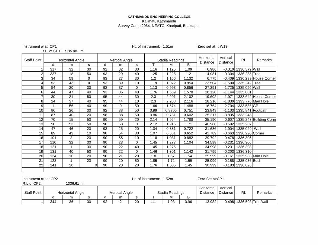
KATHMANDU ENGINEERING COLLEGE Kalimati, Kathmandu
Survey Camp 2064, NEATC, Kharipati, Bhaktapur
Instrument atat: CP1 1.51m Zero set at : W191336.304 m
d m s d m s T M B1 317 32 30 92 32 30 1.16 1.125 1.09 6.986 -0.310 1336.379 Wall2 337 18 50 93 29 40 1.25 1.225 1.2 4.981 -0.304 1336.285 Tree3 34 59 0 93 27 30 1.2 1.166 1.132 6.775 -0.409 1336.239 House Corner4 53 43 0 93 39 10 1.19 1.072 0.954 23.504 -1.500 1335.242 Tree5 54 20 30 93 37 0 1.13 0.993 0.856 27.291 -1.725 1335.096 Wall6 44 47 40 93 36 40 1.76 1.669 1.578 18.128 -1.144 1335.001 "7 30 21 50 95 44 30 2.3 2.201 2.102 19.602 -1.971 1333.642 House Corner8 24 37 40 95 44 10 2.3 2.208 2.116 18.216 -1.830 1333.776 Man Hole9 1 56 40 99 9 50 1.66 1.574 1.488 16.764 -2.704 1333.536 GP
10 86 26 30 92 38 50 0.99 0.8705 0.751 23.849 -1.103 1335.841 Footpath11 87 40 20 98 38 50 0.86 0.731 0.602 25.217 -3.835 1333.248 "12 70 15 50 90 59 20 2.14 1.964 1.788 35.190 -0.607 1335.243 Building Corne13 58 53 50 90 58 0 2.12 1.915 1.71 40.988 -0.692 1335.207 "14 47 46 20 93 26 20 1.04 0.881 0.722 31.686 -1.904 1335.029 Wall15 89 43 10 90 54 30 1.07 0.861 0.652 41.789 -0.663 1336.290 Corner16 101 2 20 90 55 10 1.18 1.031 0.882 29.792 -0.478 1336.305 "17 110 32 30 90 23 0 1.45 1.277 1.104 34.598 -0.231 1336.306 "18 121 1 30 90 22 40 1.45 1.275 1.1 34.998 -0.231 1336.308 "19 131 40 50 90 22 0 1.46 1.301 1.142 31.799 -0.203 1336.310 "20 134 10 20 90 21 20 1.8 1.67 1.54 25.999 -0.161 1335.983 Man Hole21 128 1 20 90 20 50 1.85 1.72 1.59 25.999 -0.158 1335.936 Bush22 141 20 0 90 20 20 1.76 1.605 1.45 30.999 -0.183 1336.026 "
Instrument atat : CP2 1.52m Zero Set at:CP1R.L.of CP2: 1336.61 m
Staff PointHorizontal Distance
Vertical Distance RL Remarks
d m s d m s T M B1 344 36 30 92 2 20 1.1 1.03 0.96 13.982 -0.498 1336.598 Tree/wall
RemarksStaff Point
R.L. of CP1:
Vertical Distance
Horizontal Distance RL
Ht. of instrument:
Horizontal Angle Vertical Angle Stadia Readings
Horizontal Angle Vertical Angle Stadia Readings
Ht. of instrument:
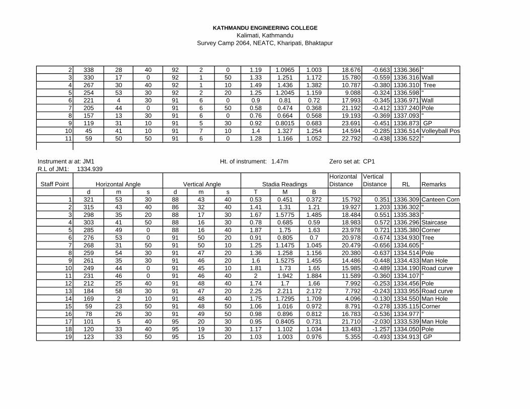
KATHMANDU ENGINEERING COLLEGE Kalimati, Kathmandu
Survey Camp 2064, NEATC, Kharipati, Bhaktapur
2 338 28 40 92 2 0 1.19 1.0965 1.003 18.676 -0.663 1336.366 "3 330 17 0 92 1 50 1.33 1.251 1.172 15.780 -0.559 1336.316 Wall4 267 30 40 92 1 10 1.49 1.436 1.382 10.787 -0.380 1336.310 Tree5 254 53 30 92 2 20 1.25 1.2045 1.159 9.088 -0.324 1336.598 "6 221 4 30 91 6 0 0.9 0.81 0.72 17.993 -0.345 1336.971 Wall7 205 44 0 91 6 50 0.58 0.474 0.368 21.192 -0.412 1337.240 Pole8 157 13 30 91 6 0 0.76 0.664 0.568 19.193 -0.369 1337.093 "9 119 31 10 91 5 30 0.92 0.8015 0.683 23.691 -0.451 1336.873 GP
10 45 41 10 91 7 10 1.4 1.327 1.254 14.594 -0.285 1336.514 Volleyball Pos11 59 50 50 91 6 0 1.28 1.166 1.052 22.792 -0.438 1336.522 "
Instrument atat: JM1 1.47m Zero set at: CP1R.L of JM1: 1334.939
Staff PointHorizontal Distance
Vertical Distance RL Remarks
d m s d m s T M B1 321 53 30 88 43 40 0.53 0.451 0.372 15.792 0.351 1336.309 Canteen Corne2 315 43 40 86 32 40 1.41 1.31 1.21 19.927 1.203 1336.302 "3 298 35 20 88 17 30 1.67 1.5775 1.485 18.484 0.551 1335.383 "4 303 41 50 88 16 30 0.78 0.685 0.59 18.983 0.572 1336.296 Staircase5 285 49 0 88 16 40 1.87 1.75 1.63 23.978 0.721 1335.380 Corner6 276 53 0 91 50 20 0.91 0.805 0.7 20.978 -0.674 1334.930 Tree7 268 31 50 91 50 10 1.25 1.1475 1.045 20.479 -0.656 1334.605 "8 259 54 30 91 47 20 1.36 1.258 1.156 20.380 -0.637 1334.514 Pole9 261 35 30 91 46 20 1.6 1.5275 1.455 14.486 -0.448 1334.433 Man Hole
10 249 44 0 91 45 10 1.81 1.73 1.65 15.985 -0.489 1334.190 Road curve11 231 46 0 91 46 40 2 1.942 1.884 11.589 -0.360 1334.107 "12 212 25 40 91 48 40 1.74 1.7 1.66 7.992 -0.253 1334.456 Pole13 184 58 30 91 47 20 2.25 2.211 2.172 7.792 -0.243 1333.955 Road curve14 169 2 10 91 48 40 1.75 1.7295 1.709 4.096 -0.130 1334.550 Man Hole15 59 23 50 91 48 50 1.06 1.016 0.972 8.791 -0.278 1335.115 Corner16 78 26 30 91 49 50 0.98 0.896 0.812 16.783 -0.536 1334.977 "17 101 5 40 95 20 30 0.95 0.8405 0.731 21.710 -2.030 1333.539 Man Hole18 120 33 40 95 19 30 1.17 1.102 1.034 13.483 -1.257 1334.050 Pole19 123 33 50 95 15 20 1.03 1.003 0.976 5.355 -0.493 1334.913 GP
Ht. of instrument:
Horizontal Angle Vertical Angle Stadia Readings
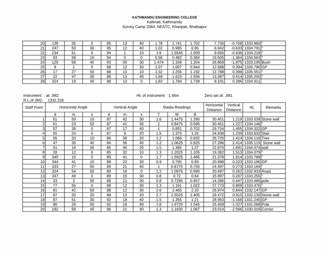
KATHMANDU ENGINEERING COLLEGE Kalimati, Kathmandu
Survey Camp 2064, NEATC, Kharipati, Bhaktapur
20 139 35 0 95 13 40 1.78 1.741 1.702 7.735 -0.708 1333.960 "21 247 50 30 95 12 40 1.02 0.985 0.95 6.942 -0.633 1334.791 "22 234 51 0 94 1 10 1.6 1.5545 1.509 9.055 -0.636 1334.218 "23 93 58 10 94 0 0 0.58 0.482 0.384 19.505 -1.364 1334.563 "24 129 58 40 93 59 30 1.474 1.339 1.204 26.869 -1.875 1333.195 Bush25 8 1 0 88 12 30 1.07 1.007 0.944 12.588 0.394 1335.796 GP26 17 27 50 88 13 10 1.32 1.256 1.192 12.788 0.398 1335.551 "27 22 47 30 88 13 40 1.69 1.623 1.556 13.387 0.414 1335.200 "28 324 19 40 88 13 0 1.83 1.784 1.738 9.191 0.286 1334.911
Instrument : at: JM2 1.45m Zero set at: JM1R.L.of JM2: 1332.318
Staff Point Horizontal Distance
Vertical Distance RL Remarks
d m s d m s T M B1 61 50 10 87 42 30 1.6 1.4475 1.295 30.451 1.219 1333.539 Stone wall2 61 23 50 87 41 30 1 0.8475 0.695 30.451 1.227 1334.148 "3 57 39 0 87 17 40 1 0.851 0.702 29.734 1.405 1334.322 GP4 55 24 0 87 9 20 1.5 1.375 1.25 24.938 1.239 1333.632 Stair5 55 33 10 86 58 20 1.2 1.066 0.932 26.725 1.414 1334.116 Tree6 47 35 40 84 56 40 1.2 1.0625 0.925 27.286 2.414 1335.119 Stone wall7 51 16 30 85 46 20 1.5 1.385 1.27 22.875 1.691 1334.074 wall8 28 12 0 85 32 10 1.3 1.2025 1.105 19.382 1.513 1334.079 "9 345 10 0 85 41 0 1.7 1.5925 1.485 21.378 1.614 1333.789 "
10 344 41 10 89 23 30 0.9 0.795 0.69 20.998 0.223 1333.196 GP11 333 27 50 89 21 40 1 0.8775 0.755 24.497 0.273 1333.164 "12 324 54 50 89 16 0 1.2 1.0975 0.995 20.497 0.262 1332.933 Road13 347 49 0 89 15 30 0.8 0.72 0.64 15.997 0.207 1333.255 "14 33 3 50 88 12 30 0.8 0.7285 0.657 14.286 0.447 1333.486 pole15 77 55 0 88 12 30 1.3 1.161 1.022 27.773 0.869 1333.476 "16 81 42 50 88 12 30 2.6 2.465 2.33 26.974 0.844 1332.147 GP17 87 20 20 88 13 20 2.7 2.5525 2.405 29.472 0.915 1332.130 Stone wall18 87 51 30 92 18 40 1.5 1.355 1.21 28.953 -1.168 1331.245 GP19 90 26 50 92 18 40 1.8 1.6725 1.545 25.459 -1.027 1331.068 Pole20 192 59 40 96 21 40 1.3 1.1835 1.067 23.014 -2.566 1330.019 Corner
Ht. of instrument:
Horizontal Angle Vertical Angle Stadia Readings
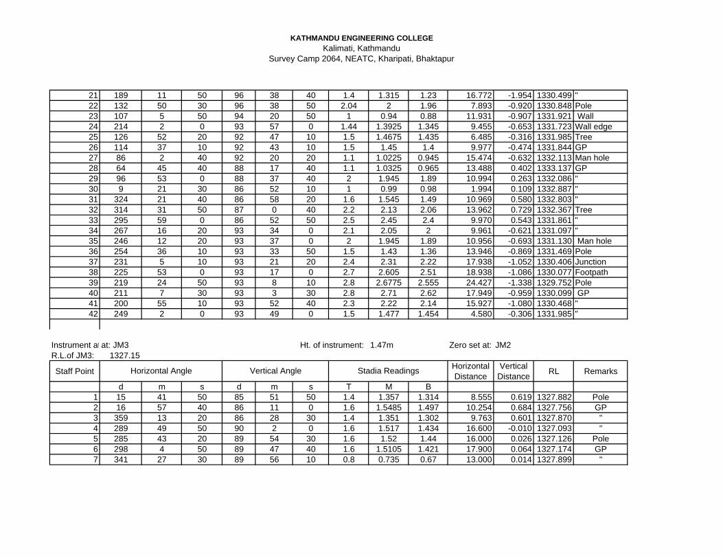
KATHMANDU ENGINEERING COLLEGE Kalimati, Kathmandu
Survey Camp 2064, NEATC, Kharipati, Bhaktapur
21 189 11 50 96 38 40 1.4 1.315 1.23 16.772 -1.954 1330.499 "22 132 50 30 96 38 50 2.04 2 1.96 7.893 -0.920 1330.848 Pole23 107 5 50 94 20 50 1 0.94 0.88 11.931 -0.907 1331.921 Wall24 214 2 0 93 57 0 1.44 1.3925 1.345 9.455 -0.653 1331.723 Wall edge25 126 52 20 92 47 10 1.5 1.4675 1.435 6.485 -0.316 1331.985 Tree26 114 37 10 92 43 10 1.5 1.45 1.4 9.977 -0.474 1331.844 GP27 86 2 40 92 20 20 1.1 1.0225 0.945 15.474 -0.632 1332.113 Man hole28 64 45 40 88 17 40 1.1 1.0325 0.965 13.488 0.402 1333.137 GP29 96 53 0 88 37 40 2 1.945 1.89 10.994 0.263 1332.086 "30 9 21 30 86 52 10 1 0.99 0.98 1.994 0.109 1332.887 "31 324 21 40 86 58 20 1.6 1.545 1.49 10.969 0.580 1332.803 "32 314 31 50 87 0 40 2.2 2.13 2.06 13.962 0.729 1332.367 Tree33 295 59 0 86 52 50 2.5 2.45 2.4 9.970 0.543 1331.861 "34 267 16 20 93 34 0 2.1 2.05 2 9.961 -0.621 1331.097 "35 246 12 20 93 37 0 2 1.945 1.89 10.956 -0.693 1331.130 Man hole36 254 36 10 93 33 50 1.5 1.43 1.36 13.946 -0.869 1331.469 Pole37 231 5 10 93 21 20 2.4 2.31 2.22 17.938 -1.052 1330.406 Junction38 225 53 0 93 17 0 2.7 2.605 2.51 18.938 -1.086 1330.077 Footpath39 219 24 50 93 8 10 2.8 2.6775 2.555 24.427 -1.338 1329.752 Pole40 211 7 30 93 3 30 2.8 2.71 2.62 17.949 -0.959 1330.099 GP41 200 55 10 93 52 40 2.3 2.22 2.14 15.927 -1.080 1330.468 "42 249 2 0 93 49 0 1.5 1.477 1.454 4.580 -0.306 1331.985 "
Instrument atat: JM3 1.47m Zero set at: JM2R.L.of JM3: 1327.15
Staff Point Horizontal Distance
Vertical Distance RL Remarks
d m s d m s T M B1 15 41 50 85 51 50 1.4 1.357 1.314 8.555 0.619 1327.882 Pole2 16 57 40 86 11 0 1.6 1.5485 1.497 10.254 0.684 1327.756 GP3 359 13 20 86 28 30 1.4 1.351 1.302 9.763 0.601 1327.870 "4 289 49 50 90 2 0 1.6 1.517 1.434 16.600 -0.010 1327.093 "5 285 43 20 89 54 30 1.6 1.52 1.44 16.000 0.026 1327.126 Pole6 298 4 50 89 47 40 1.6 1.5105 1.421 17.900 0.064 1327.174 GP7 341 27 30 89 56 10 0.8 0.735 0.67 13.000 0.014 1327.899 "
Ht. of instrument:
Horizontal Angle Vertical Angle Stadia Readings
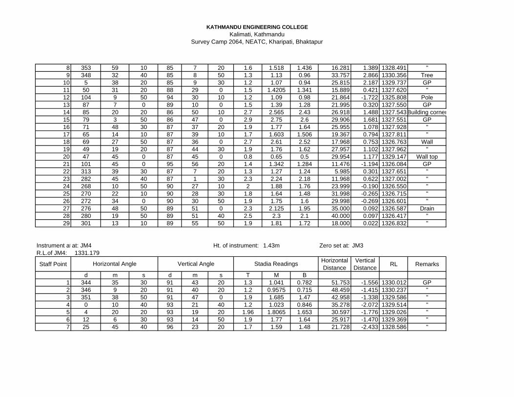
KATHMANDU ENGINEERING COLLEGE Kalimati, Kathmandu
Survey Camp 2064, NEATC, Kharipati, Bhaktapur
8 353 59 10 85 7 20 1.6 1.518 1.436 16.281 1.389 1328.491 "9 348 32 40 85 8 50 1.3 1.13 0.96 33.757 2.866 1330.356 Tree
10 5 38 20 85 9 30 1.2 1.07 0.94 25.815 2.187 1329.737 GP11 50 31 20 88 29 0 1.5 1.4205 1.341 15.889 0.421 1327.620 "12 104 9 50 94 30 10 1.2 1.09 0.98 21.864 -1.722 1325.808 Pole13 87 7 0 89 10 0 1.5 1.39 1.28 21.995 0.320 1327.550 GP14 85 20 20 86 50 10 2.7 2.565 2.43 26.918 1.488 1327.543Building corner15 79 3 50 86 47 0 2.9 2.75 2.6 29.906 1.681 1327.551 GP16 71 48 30 87 37 20 1.9 1.77 1.64 25.955 1.078 1327.928 "17 65 14 10 87 39 10 1.7 1.603 1.506 19.367 0.794 1327.811 "18 69 27 50 87 36 0 2.7 2.61 2.52 17.968 0.753 1326.763 Wall19 49 19 20 87 44 30 1.9 1.76 1.62 27.957 1.102 1327.962 "20 47 45 0 87 45 0 0.8 0.65 0.5 29.954 1.177 1329.147 Wall top21 101 45 0 95 56 20 1.4 1.342 1.284 11.476 -1.194 1326.084 GP22 313 39 30 87 7 20 1.3 1.27 1.24 5.985 0.301 1327.651 "23 282 45 40 87 1 30 2.3 2.24 2.18 11.968 0.622 1327.002 "24 268 10 50 90 27 10 2 1.88 1.76 23.999 -0.190 1326.550 "25 270 22 10 90 28 30 1.8 1.64 1.48 31.998 -0.265 1326.715 "26 272 34 0 90 30 50 1.9 1.75 1.6 29.998 -0.269 1326.601 "27 276 48 50 89 51 0 2.3 2.125 1.95 35.000 0.092 1326.587 Drain28 280 19 50 89 51 40 2.5 2.3 2.1 40.000 0.097 1326.417 "29 301 13 10 89 55 50 1.9 1.81 1.72 18.000 0.022 1326.832 "
Instrument atat: JM4 1.43m Zero set at: JM3R.L.of JM4: 1331.179
Staff Point Horizontal Distance
Vertical Distance RL Remarks
d m s d m s T M B1 344 35 30 91 43 20 1.3 1.041 0.782 51.753 -1.556 1330.012 GP2 346 9 20 91 40 20 1.2 0.9575 0.715 48.459 -1.415 1330.237 "3 351 38 50 91 47 0 1.9 1.685 1.47 42.958 -1.338 1329.586 "4 0 10 40 93 21 40 1.2 1.023 0.846 35.278 -2.072 1329.514 "5 4 20 20 93 19 20 1.96 1.8065 1.653 30.597 -1.776 1329.026 "6 12 6 30 93 14 50 1.9 1.77 1.64 25.917 -1.470 1329.369 "7 25 45 40 96 23 20 1.7 1.59 1.48 21.728 -2.433 1328.586 "
Ht. of instrument:
Horizontal Angle Vertical Angle Stadia Readings
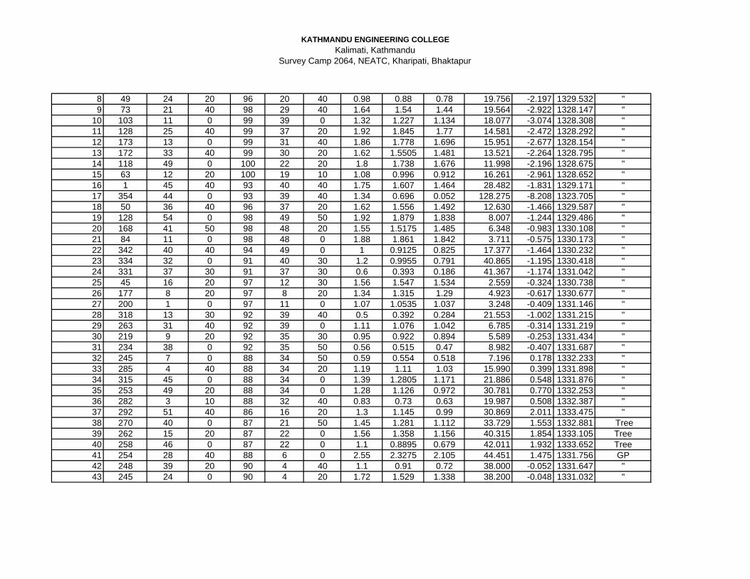
KATHMANDU ENGINEERING COLLEGE Kalimati, Kathmandu
Survey Camp 2064, NEATC, Kharipati, Bhaktapur
8 49 24 20 96 20 40 0.98 0.88 0.78 19.756 -2.197 1329.532 "9 73 21 40 98 29 40 1.64 1.54 1.44 19.564 -2.922 1328.147 "
10 103 11 0 99 39 0 1.32 1.227 1.134 18.077 -3.074 1328.308 "11 128 25 40 99 37 20 1.92 1.845 1.77 14.581 -2.472 1328.292 "12 173 13 0 99 31 40 1.86 1.778 1.696 15.951 -2.677 1328.154 "13 172 33 40 99 30 20 1.62 1.5505 1.481 13.521 -2.264 1328.795 "14 118 49 0 100 22 20 1.8 1.738 1.676 11.998 -2.196 1328.675 "15 63 12 20 100 19 10 1.08 0.996 0.912 16.261 -2.961 1328.652 "16 1 45 40 93 40 40 1.75 1.607 1.464 28.482 -1.831 1329.171 "17 354 44 0 93 39 40 1.34 0.696 0.052 128.275 -8.208 1323.705 "18 50 36 40 96 37 20 1.62 1.556 1.492 12.630 -1.466 1329.587 "19 128 54 0 98 49 50 1.92 1.879 1.838 8.007 -1.244 1329.486 "20 168 41 50 98 48 20 1.55 1.5175 1.485 6.348 -0.983 1330.108 "21 84 11 0 98 48 0 1.88 1.861 1.842 3.711 -0.575 1330.173 "22 342 40 40 94 49 0 1 0.9125 0.825 17.377 -1.464 1330.232 "23 334 32 0 91 40 30 1.2 0.9955 0.791 40.865 -1.195 1330.418 "24 331 37 30 91 37 30 0.6 0.393 0.186 41.367 -1.174 1331.042 "25 45 16 20 97 12 30 1.56 1.547 1.534 2.559 -0.324 1330.738 "26 177 8 20 97 8 20 1.34 1.315 1.29 4.923 -0.617 1330.677 "27 200 1 0 97 11 0 1.07 1.0535 1.037 3.248 -0.409 1331.146 "28 318 13 30 92 39 40 0.5 0.392 0.284 21.553 -1.002 1331.215 "29 263 31 40 92 39 0 1.11 1.076 1.042 6.785 -0.314 1331.219 "30 219 9 20 92 35 30 0.95 0.922 0.894 5.589 -0.253 1331.434 "31 234 38 0 92 35 50 0.56 0.515 0.47 8.982 -0.407 1331.687 "32 245 7 0 88 34 50 0.59 0.554 0.518 7.196 0.178 1332.233 "33 285 4 40 88 34 20 1.19 1.11 1.03 15.990 0.399 1331.898 "34 315 45 0 88 34 0 1.39 1.2805 1.171 21.886 0.548 1331.876 "35 253 49 20 88 34 0 1.28 1.126 0.972 30.781 0.770 1332.253 "36 282 3 10 88 32 40 0.83 0.73 0.63 19.987 0.508 1332.387 "37 292 51 40 86 16 20 1.3 1.145 0.99 30.869 2.011 1333.475 "38 270 40 0 87 21 50 1.45 1.281 1.112 33.729 1.553 1332.881 Tree39 262 15 20 87 22 0 1.56 1.358 1.156 40.315 1.854 1333.105 Tree40 258 46 0 87 22 0 1.1 0.8895 0.679 42.011 1.932 1333.652 Tree41 254 28 40 88 6 0 2.55 2.3275 2.105 44.451 1.475 1331.756 GP42 248 39 20 90 4 40 1.1 0.91 0.72 38.000 -0.052 1331.647 "43 245 24 0 90 4 20 1.72 1.529 1.338 38.200 -0.048 1331.032 "
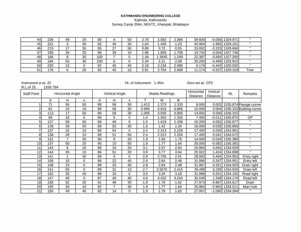
KATHMANDU ENGINEERING COLLEGE Kalimati, Kathmandu
Survey Camp 2064, NEATC, Kharipati, Bhaktapur
44 236 49 20 90 4 50 2.78 2.582 2.384 39.600 -0.056 1329.971 "45 231 3 30 92 46 30 1.64 1.435 1.23 40.904 -1.983 1329.191 "46 219 17 30 95 27 50 0.89 0.72 0.55 33.692 -3.223 1328.666 "47 189 26 20 98 39 10 1.96 1.859 1.758 19.743 -3.004 1327.746 "48 186 8 30 100 7 0 1.48 1.3645 1.249 22.387 -3.994 1327.250 "49 184 50 30 100 6 0 2.34 2.21 2.08 25.200 -4.489 1325.910 "50 220 13 0 92 45 40 2.18 2.134 2.088 9.179 -0.443 1330.032 "51 176 6 20 92 45 10 2.81 2.754 2.698 11.174 -0.537 1329.318 Tree
Instrument atat: J3 1.45m Zero set at: CP2R.L.of J3: 1335.794
Staff Point Horizontal Distance
Vertical Distance RL Remarks
d m s d m s T M B1 71 56 50 89 58 30 1.413 1.373 1.333 8.000 0.003 1335.874 Passge corner2 81 15 10 89 58 30 0.966 0.916 0.866 10.000 0.004 1336.332Building corner3 113 17 50 89 58 30 1.005 0.935 0.865 14.000 0.006 1336.315 "4 69 16 0 90 5 0 1.4 1.363 1.326 7.400 -0.011 1335.870 GP5 127 58 50 89 49 0 1.5 1.419 1.338 16.200 0.052 1335.877 "6 128 39 20 89 52 30 1.5 1.42 1.34 16.000 0.035 1335.859 "7 137 32 10 89 54 0 2.4 2.313 2.226 17.400 0.030 1334.961 "8 138 28 10 89 51 50 2.4 2.313 2.226 17.400 0.041 1334.972 "9 131 7 30 90 8 20 1.9 1.83 1.76 14.000 -0.034 1335.380 "
10 137 50 20 90 10 50 1.9 1.77 1.64 26.000 -0.082 1335.392 "11 144 6 20 88 33 20 3.1 2.97 2.84 25.983 0.655 1334.929 "12 144 35 10 86 51 20 3.9 3.77 3.64 25.922 1.424 1334.898 "13 141 1 30 89 5 0 2.9 2.755 2.61 28.993 0.464 1334.953 Entry right14 158 15 0 89 22 40 2.8 2.64 2.48 31.996 0.347 1334.951 Entry left15 138 23 0 89 25 30 2.8 2.64 2.48 31.997 0.321 1334.925 Drain right16 141 55 0 89 31 10 2.7 2.5575 2.415 28.498 0.239 1334.926 Drain left17 152 30 40 89 33 0 3.5 3.34 3.18 31.998 0.251 1334.155 Road right18 147 49 0 87 49 40 4.6 4.422 4.244 35.549 1.348 1334.170 Road left19 156 52 20 91 46 30 1.9 1.76 1.62 27.973 -0.867 1334.617 Drain20 155 30 10 92 7 30 1.9 1.77 1.64 25.964 -0.963 1334.511 Man hole21 150 49 40 92 14 0 1.9 1.76 1.62 27.957 -1.090 1334.394 "
Ht. of instrument:
Horizontal Angle Vertical Angle Stadia Readings
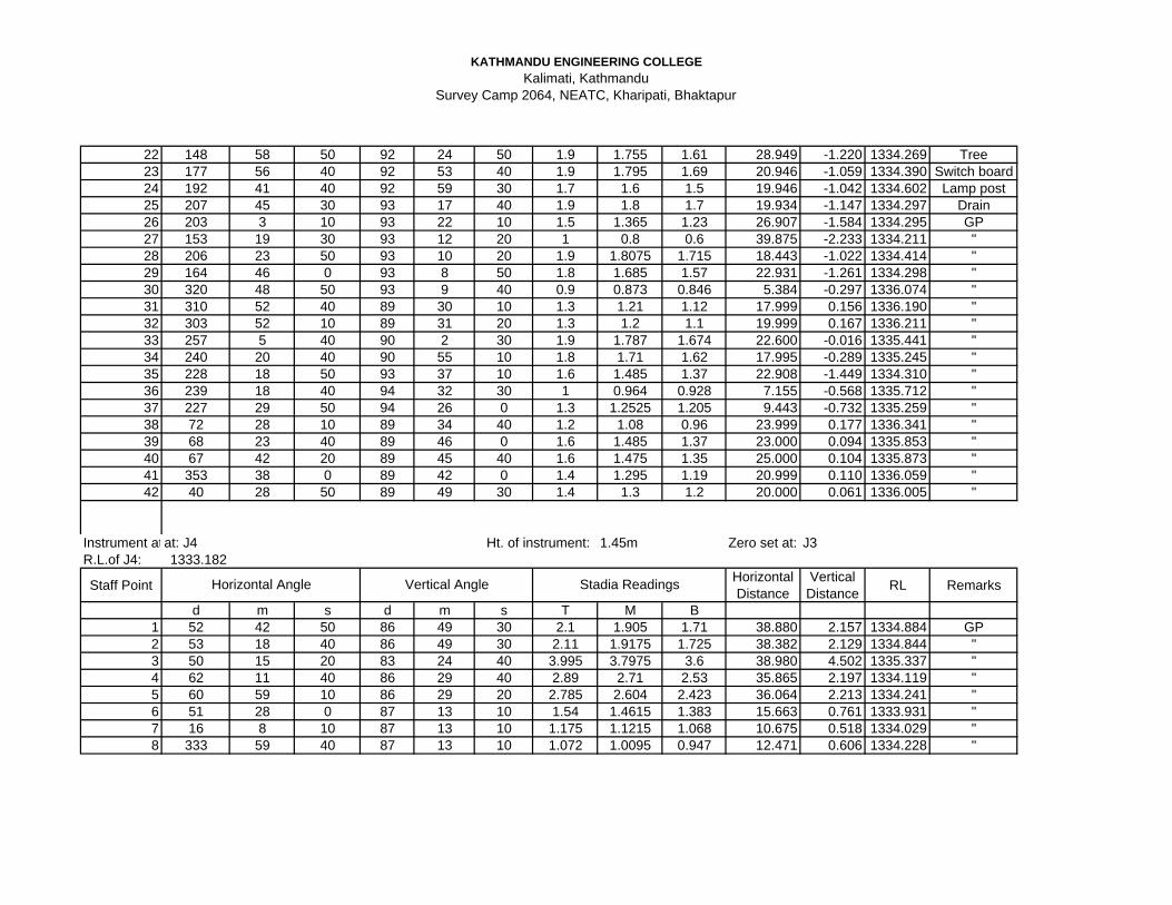
KATHMANDU ENGINEERING COLLEGE Kalimati, Kathmandu
Survey Camp 2064, NEATC, Kharipati, Bhaktapur
22 148 58 50 92 24 50 1.9 1.755 1.61 28.949 -1.220 1334.269 Tree23 177 56 40 92 53 40 1.9 1.795 1.69 20.946 -1.059 1334.390 Switch board24 192 41 40 92 59 30 1.7 1.6 1.5 19.946 -1.042 1334.602 Lamp post25 207 45 30 93 17 40 1.9 1.8 1.7 19.934 -1.147 1334.297 Drain26 203 3 10 93 22 10 1.5 1.365 1.23 26.907 -1.584 1334.295 GP27 153 19 30 93 12 20 1 0.8 0.6 39.875 -2.233 1334.211 "28 206 23 50 93 10 20 1.9 1.8075 1.715 18.443 -1.022 1334.414 "29 164 46 0 93 8 50 1.8 1.685 1.57 22.931 -1.261 1334.298 "30 320 48 50 93 9 40 0.9 0.873 0.846 5.384 -0.297 1336.074 "31 310 52 40 89 30 10 1.3 1.21 1.12 17.999 0.156 1336.190 "32 303 52 10 89 31 20 1.3 1.2 1.1 19.999 0.167 1336.211 "33 257 5 40 90 2 30 1.9 1.787 1.674 22.600 -0.016 1335.441 "34 240 20 40 90 55 10 1.8 1.71 1.62 17.995 -0.289 1335.245 "35 228 18 50 93 37 10 1.6 1.485 1.37 22.908 -1.449 1334.310 "36 239 18 40 94 32 30 1 0.964 0.928 7.155 -0.568 1335.712 "37 227 29 50 94 26 0 1.3 1.2525 1.205 9.443 -0.732 1335.259 "38 72 28 10 89 34 40 1.2 1.08 0.96 23.999 0.177 1336.341 "39 68 23 40 89 46 0 1.6 1.485 1.37 23.000 0.094 1335.853 "40 67 42 20 89 45 40 1.6 1.475 1.35 25.000 0.104 1335.873 "41 353 38 0 89 42 0 1.4 1.295 1.19 20.999 0.110 1336.059 "42 40 28 50 89 49 30 1.4 1.3 1.2 20.000 0.061 1336.005 "
Instrument atat: J4 1.45m Zero set at: J3R.L.of J4: 1333.182
Staff Point Horizontal Distance
Vertical Distance RL Remarks
d m s d m s T M B1 52 42 50 86 49 30 2.1 1.905 1.71 38.880 2.157 1334.884 GP2 53 18 40 86 49 30 2.11 1.9175 1.725 38.382 2.129 1334.844 "3 50 15 20 83 24 40 3.995 3.7975 3.6 38.980 4.502 1335.337 "4 62 11 40 86 29 40 2.89 2.71 2.53 35.865 2.197 1334.119 "5 60 59 10 86 29 20 2.785 2.604 2.423 36.064 2.213 1334.241 "6 51 28 0 87 13 10 1.54 1.4615 1.383 15.663 0.761 1333.931 "7 16 8 10 87 13 10 1.175 1.1215 1.068 10.675 0.518 1334.029 "8 333 59 40 87 13 10 1.072 1.0095 0.947 12.471 0.606 1334.228 "
Ht. of instrument:
Horizontal Angle Vertical Angle Stadia Readings
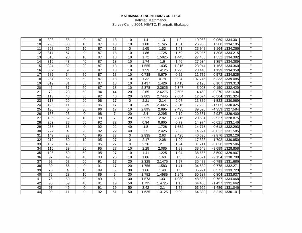
KATHMANDU ENGINEERING COLLEGE Kalimati, Kathmandu
Survey Camp 2064, NEATC, Kharipati, Bhaktapur
9 303 56 0 87 13 10 1.4 1.3 1.2 19.953 0.969 1334.301 "10 296 30 10 87 13 10 1.88 1.745 1.61 26.936 1.308 1334.195 "11 303 25 10 87 13 0 1.65 1.53 1.41 23.943 1.164 1334.266 "12 314 57 0 87 13 10 1.86 1.725 1.59 26.936 1.308 1334.215 "13 316 23 10 87 13 10 1.72 1.5825 1.445 27.435 1.332 1334.382 "14 319 43 40 87 13 10 1.74 1.6 1.46 27.934 1.357 1334.389 "15 324 32 20 87 13 10 1.555 1.435 1.315 23.944 1.163 1334.360 "16 332 9 0 87 13 10 1.53 1.4125 1.295 23.445 1.139 1334.358 "17 382 34 50 87 13 10 0.738 0.679 0.62 11.772 0.572 1334.525 "18 284 55 50 87 13 10 1.32 0.78 0.24 107.746 5.233 1339.085 "19 319 31 50 87 13 10 1.437 1.426 1.415 2.195 0.107 1333.313 "20 46 37 50 87 13 10 2.378 2.3625 2.347 3.093 0.150 1332.420 "21 72 23 50 94 44 20 2.65 2.6275 2.605 4.469 -0.370 1331.634 "22 113 48 30 92 40 20 2.805 2.7445 2.684 12.074 -0.564 1331.324 "23 118 29 20 96 17 0 2.21 2.14 2.07 13.832 -1.523 1330.969 "24 126 11 20 96 17 10 2.39 2.3025 2.215 17.290 -1.905 1330.425 "25 130 6 30 96 17 10 2.895 2.695 2.495 39.520 -4.353 1327.584 "26 133 23 0 98 7 20 2.4 2.295 2.19 20.581 -2.937 1329.400 "27 136 52 10 98 7 20 2.925 2.82 2.715 20.581 -2.937 1328.875 "28 259 23 50 92 22 30 0.94 0.865 0.79 14.974 -0.621 1333.146 "29 238 16 0 92 22 40 1.8 1.726 1.652 14.775 -0.613 1332.293 "30 227 4 20 92 22 40 2.5 2.425 2.35 14.974 -0.622 1331.585 "31 142 32 40 95 27 0 2.835 2.63 2.425 40.630 -3.876 1328.126 "32 212 50 10 95 27 0 2.17 2.08 1.99 17.838 -1.702 1330.850 "33 167 46 0 95 27 0 2.26 2.1 1.94 31.711 -3.026 1329.506 "34 110 39 30 95 27 10 2.28 2.085 1.89 38.648 -3.689 1328.858 "35 103 59 50 95 27 10 1.41 1.225 1.04 36.666 -3.500 1329.907 "36 97 49 40 93 26 10 1.86 1.68 1.5 35.871 -2.154 1330.798 "37 92 53 50 91 17 20 2.325 2.1475 1.97 35.482 -0.798 1331.686 "38 80 56 0 91 17 20 1.756 1.583 1.41 34.582 -0.778 1332.271 "39 76 4 10 89 5 30 1.66 1.48 1.3 35.991 0.571 1333.723 "40 76 28 10 89 5 30 1.752 1.4985 1.245 50.687 0.804 1333.937 "41 75 50 50 89 5 30 1.573 1.331 1.089 48.388 0.767 1334.068 "42 96 59 40 91 19 50 1.795 1.4725 1.15 64.465 -1.497 1331.662 "43 97 49 0 91 19 50 2.42 2.1 1.78 63.965 -1.486 1331.046 "44 99 11 0 92 51 50 1.635 1.3125 0.99 64.339 -3.219 1330.101 "

KATHMANDU ENGINEERING COLLEGE Kalimati, Kathmandu
Survey Camp 2064, NEATC, Kharipati, Bhaktapur
Instrument at: J6 1.45m Zero set at: J5R.L.of J6: 1326.843 m
Staff Point Horizontal Distance
Vertical Distance RL Remarks
1 d m s d m s T M B2 62 56 20 87 30 10 1.33 1.005 0.68 64.877 2.829 1330.117 GP3 62 48 40 87 30 10 1.75 1.4565 1.163 58.589 2.555 1329.392 "4 64 11 30 87 30 10 2.285 2.0375 1.79 49.406 2.155 1328.410 "5 66 9 10 87 30 0 2.915 2.665 2.415 49.905 2.179 1327.807 "6 66 31 30 88 24 10 2.61 2.3725 2.135 47.463 1.323 1327.244 "7 79 44 0 89 9 50 2.62 2.46 2.3 31.993 0.467 1326.300 "8 41 58 0 87 30 50 1.854 1.6195 1.385 46.812 2.032 1328.706 "9 78 8 0 90 3 0 2.4 2.274 2.148 25.200 -0.022 1325.997 "
10 12 19 40 88 52 0 1.3 1.13 0.96 33.987 0.672 1327.835 "11 101 51 40 92 18 0 1.74 1.585 1.43 30.950 -1.243 1325.465 "12 354 50 20 88 54 0 0.83 0.66 0.49 33.987 0.653 1328.286 "13 329 39 30 88 54 0 1.43 1.2675 1.105 32.488 0.624 1327.649 "14 313 56 10 87 51 0 1.3 1.1075 0.915 38.446 1.443 1328.629 "15 337 29 40 87 51 0 1.65 1.5175 1.385 26.463 0.993 1327.769 "16 338 12 20 87 51 0 2.04 1.896 1.752 28.759 1.080 1327.477 "17 338 12 20 87 51 0 2.485 2.3525 2.22 26.463 0.993 1326.934 "18 350 25 20 87 51 0 1.962 1.836 1.71 25.165 0.945 1327.402 "19 349 13 20 87 51 0 2.39 2.2725 2.155 23.467 0.881 1326.902 "20 53 6 20 87 51 0 1.765 1.7 1.635 12.982 0.487 1327.080 "21 63 7 40 87 51 0 2.03 2 1.97 5.992 0.225 1326.518 "22 110 4 50 87 50 0 2.415 2.875 3.335 -91.869 -3.476 1321.942 "23 104 14 0 91 29 30 2.25 2.1 1.95 29.980 -0.781 1325.412 "24 123 6 50 91 29 30 2.045 2.0025 1.96 8.494 -0.221 1326.069 "25 202 23 20 91 29 30 1.673 1.6265 1.58 9.294 -0.242 1326.424 "26 218 21 30 90 0 50 2.06 1.96 1.86 20.000 -0.005 1326.328 "27 217 41 10 90 0 50 1.995 1.8275 1.66 33.500 -0.008 1326.457 "28 217 31 0 90 0 50 1.595 1.4215 1.248 34.700 -0.008 1326.863 "29 197 32 30 90 0 50 2.74 2.5725 2.405 33.500 -0.008 1325.712 "30 197 9 0 90 0 50 2.225 2.055 1.885 34.000 -0.008 1326.230 "
Ht. of instrument:
Horizontal Angle Vertical Angle Stadia Readings

KATHMANDU ENGINEERING COLLEGE Kalimati, Kathmandu
Survey Camp 2064, NEATC, Kharipati, Bhaktapur
31 197 9 0 90 2 10 2 1.8275 1.655 34.500 -0.022 1326.444 "32 197 41 10 90 2 10 2.45 2.26 2.07 38.000 -0.024 1326.009 "33 198 5 0 90 2 10 2.26 2.03 1.8 46.000 -0.029 1326.234 "34 187 29 30 90 2 20 2.515 2.341 2.167 34.800 -0.024 1325.928 "
3 at: W12 1.47m Zero set at: J6R.L. of W12:1327.774 m
Staff Point Horizontal Distance
Vertical Distance RL Remarks
d m s d m s T M B1 96 7 0 92 35 30 1.66 1.643 1.626 3.393 -0.154 1327.447 Pole2 15 58 40 92 35 30 1.487 1.4675 1.448 3.892 -0.176 1327.600 Road (Rt)3 61 16 0 92 35 30 1.865 1.8095 1.754 11.077 -0.501 1326.933 "4 65 9 0 92 35 30 2.215 2.0965 1.978 23.652 -1.071 1326.077 "5 63 4 0 92 35 30 2.38 2.193 2.006 37.324 -1.689 1325.362 "6 60 32 10 92 35 30 2.41 2.165 1.92 48.900 -2.213 1324.866 Road(Lt)7 63 9 10 92 35 30 2.415 2.1615 1.908 50.596 -2.290 1324.792 road/ pole8 68 34 30 92 36 10 2.28 2.085 1.89 38.920 -1.769 1325.390 "9 76 17 10 92 34 10 2.1 1.9935 1.887 21.257 -0.954 1326.297 GP
10 165 13 10 95 1 10 2.84 2.805 2.77 6.946 -0.610 1325.829 GP11 170 11 40 95 1 40 2.915 2.895 2.875 3.969 -0.349 1326.000 GP12 170 11 40 95 1 40 2.915 2.895 2.875 3.969 -0.349 1326.000 Wall13 114 22 10 108 54 50 1.46 1.44 1.42 3.580 -1.227 1326.577 Bamboo bush14 88 29 20 95 27 40 2.385 2.325 2.265 11.891 -1.137 1325.782 Bamboo bush15 93 57 50 96 21 0 2.465 2.36 2.255 20.743 -2.308 1324.576 GP16 82 14 30 96 21 0 1.93 1.8275 1.725 20.249 -2.253 1325.163 Bamboo bush
at: W13 1.5m Zero set at: W12m
Horizontal Distance
Vertical Distance RL Remarks
d m s d m s T M B1 345 17 40 90 34 20 1.7 1.44 1.18 51.995 -0.519 1324.185 GP2 335 7 0 90 31 0 2.2 1.945 1.69 50.996 -0.460 1323.739 "
Horizontal Angle Vertical Angle Stadia Readings
Ht. of instrument:
Horizontal Angle Vertical Angle Stadia Readings
Ht. of instrument:

KATHMANDU ENGINEERING COLLEGE Kalimati, Kathmandu
Survey Camp 2064, NEATC, Kharipati, Bhaktapur
3 331 2 40 90 27 10 2.9 2.702 2.504 39.598 -0.313 1323.129 "4 227 0 40 92 6 0 2.1 1.92 1.74 35.952 -1.318 1322.906 "5 306 38 30 92 5 50 2.82 2.672 2.524 29.560 -1.082 1322.390 "6 266 41 30 95 42 10 2.7 2.605 2.51 18.812 -1.879 1321.660 "7 242 28 40 95 36 30 2.2 2.0565 1.913 28.426 -2.791 1321.296 "8 227 10 10 94 40 30 1.8 1.482 1.164 63.178 -5.166 1319.496 "9 326 27 40 94 38 10 3.5 3.4065 3.313 18.578 -1.507 1321.231 Pond 1
10 339 48 50 94 21 40 1 0.905 0.81 18.890 -1.441 1323.798 GP11 363 31 10 92 56 30 1.68 1.604 1.528 15.160 -0.779 1323.761 GP12 324 10 10 92 56 40 2.9 2.8165 2.733 16.656 -0.857 1322.471 GP13 302 49 0 97 1 40 2.8 2.704 2.608 18.913 -2.331 1321.109 Pond 214 303 50 20 98 11 0 1.56 1.49 1.42 13.716 -1.972 1322.682 GP15 213 6 40 95 31 30 1.76 1.652 1.544 21.400 -2.070 1322.422 GP16 210 39 10 95 22 0 0.8 0.76 0.72 7.930 -0.745 1324.639 Pole17 188 34 40 89 43 30 1.28 1.152 1.024 25.599 0.123 1325.115 Pole18 185 46 0 89 43 10 0.84 0.622 0.404 43.599 0.213 1325.735 Pole19 179 12 10 89 43 20 0.9 0.69 0.48 41.999 0.204 1325.658 GP20 177 44 0 89 43 20 1.37 1.253 1.136 23.399 0.113 1325.004 "21 74 31 30 89 39 10 1.52 1.484 1.448 7.200 0.044 1324.704 "22 88 9 30 89 39 10 0.81 0.745 0.68 13.000 0.079 1325.478 "23 74 6 10 86 30 30 1.7 1.574 1.448 25.107 1.532 1326.102 "24 122 41 10 86 30 30 0.98 0.824 0.668 31.084 1.897 1327.217 "25 125 0 20 85 54 20 1.3 1.14 0.98 31.837 2.279 1327.283 "26 173 10 10 88 35 0 1.9 1.7665 1.633 26.684 0.660 1325.037 "27 170 49 10 88 37 20 1.76 1.62 1.48 27.984 0.673 1325.197 "28 163 29 10 87 37 50 1.04 0.888 0.736 30.348 1.256 1326.512 "29 155 16 20 84 15 40 1.4 1.2265 1.053 34.353 3.452 1328.370 "30 125 13 30 84 14 30 1.6 1.4205 1.241 35.539 3.584 1328.307 "31 126 12 10 83 8 40 1.9 1.7125 1.525 36.966 4.444 1328.876 "32 170 58 0 85 43 30 1.7 1.472 1.244 45.347 3.390 1328.062 "33 166 17 0 84 2 30 1.9 1.6565 1.413 48.175 5.028 1329.516 "34 152 4 50 83 30 10 1.3 1.09 0.88 41.462 4.722 1329.776 GP35 47 48 20 90 18 0 1.46 1.367 1.274 18.599 -0.097 1324.680 "36 26 14 50 90 14 50 1.2 1.052 0.904 29.599 -0.128 1324.964 "37 6 24 10 90 13 10 1.4 1.2325 1.065 33.500 -0.128 1324.783 "38 1 39 0 91 43 0 1.5 1.355 1.21 28.974 -0.868 1323.921 "
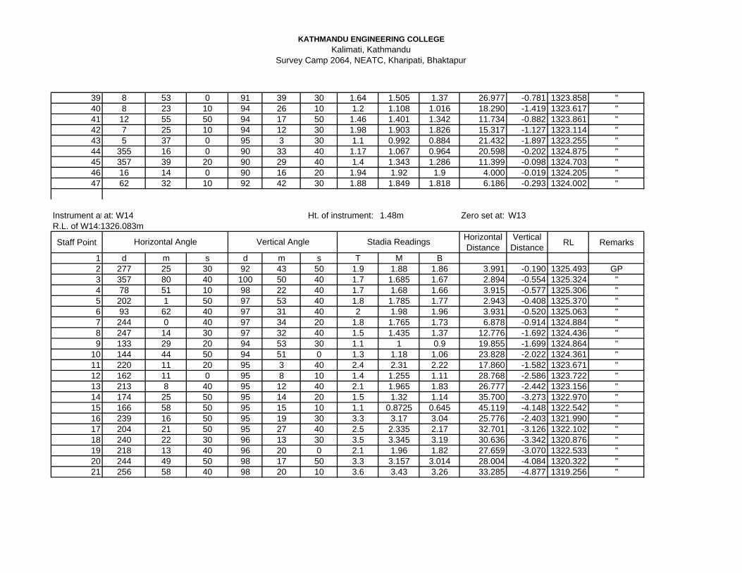
KATHMANDU ENGINEERING COLLEGE Kalimati, Kathmandu
Survey Camp 2064, NEATC, Kharipati, Bhaktapur
39 8 53 0 91 39 30 1.64 1.505 1.37 26.977 -0.781 1323.858 "40 8 23 10 94 26 10 1.2 1.108 1.016 18.290 -1.419 1323.617 "41 12 55 50 94 17 50 1.46 1.401 1.342 11.734 -0.882 1323.861 "42 7 25 10 94 12 30 1.98 1.903 1.826 15.317 -1.127 1323.114 "43 5 37 0 95 3 30 1.1 0.992 0.884 21.432 -1.897 1323.255 "44 355 16 0 90 33 40 1.17 1.067 0.964 20.598 -0.202 1324.875 "45 357 39 20 90 29 40 1.4 1.343 1.286 11.399 -0.098 1324.703 "46 16 14 0 90 16 20 1.94 1.92 1.9 4.000 -0.019 1324.205 "47 62 32 10 92 42 30 1.88 1.849 1.818 6.186 -0.293 1324.002 "
Instrument atat: W14 1.48m Zero set at: W13R.L. of W14:1326.083m
Staff Point Horizontal Distance
Vertical Distance RL Remarks
1 d m s d m s T M B2 277 25 30 92 43 50 1.9 1.88 1.86 3.991 -0.190 1325.493 GP3 357 80 40 100 50 40 1.7 1.685 1.67 2.894 -0.554 1325.324 "4 78 51 10 98 22 40 1.7 1.68 1.66 3.915 -0.577 1325.306 "5 202 1 50 97 53 40 1.8 1.785 1.77 2.943 -0.408 1325.370 "6 93 62 40 97 31 40 2 1.98 1.96 3.931 -0.520 1325.063 "7 244 0 40 97 34 20 1.8 1.765 1.73 6.878 -0.914 1324.884 "8 247 14 30 97 32 40 1.5 1.435 1.37 12.776 -1.692 1324.436 "9 133 29 20 94 53 30 1.1 1 0.9 19.855 -1.699 1324.864 "
10 144 44 50 94 51 0 1.3 1.18 1.06 23.828 -2.022 1324.361 "11 220 11 20 95 3 40 2.4 2.31 2.22 17.860 -1.582 1323.671 "12 162 11 0 95 8 10 1.4 1.255 1.11 28.768 -2.586 1323.722 "13 213 8 40 95 12 40 2.1 1.965 1.83 26.777 -2.442 1323.156 "14 174 25 50 95 14 20 1.5 1.32 1.14 35.700 -3.273 1322.970 "15 166 58 50 95 15 10 1.1 0.8725 0.645 45.119 -4.148 1322.542 "16 239 16 50 95 19 30 3.3 3.17 3.04 25.776 -2.403 1321.990 "17 204 21 50 95 27 40 2.5 2.335 2.17 32.701 -3.126 1322.102 "18 240 22 30 96 13 30 3.5 3.345 3.19 30.636 -3.342 1320.876 "19 218 13 40 96 20 0 2.1 1.96 1.82 27.659 -3.070 1322.533 "20 244 49 50 98 17 50 3.3 3.157 3.014 28.004 -4.084 1320.322 "21 256 58 40 98 20 10 3.6 3.43 3.26 33.285 -4.877 1319.256 "
Ht. of instrument:
Horizontal Angle Vertical Angle Stadia Readings

KATHMANDU ENGINEERING COLLEGE Kalimati, Kathmandu
Survey Camp 2064, NEATC, Kharipati, Bhaktapur
22 208 30 10 102 20 10 2.7 2.587 2.474 21.568 -4.717 1320.259 "23 318 20 40 102 14 20 1.3 1.2 1.1 19.101 -4.143 1322.220 GP24 315 47 50 102 12 50 1.8 1.69 1.58 21.015 -4.549 1321.324 "25 315 18 10 102 23 20 2.4 2.29 2.18 20.987 -4.610 1320.663 "26 270 50 10 102 30 50 2.4 2.3 2.2 19.061 -4.231 1321.032 "27 247 9 50 102 21 0 1 0.865 0.73 25.765 -5.641 1321.057 "28 90 25 10 90 54 0 2.3 2.259 2.218 8.198 -0.129 1325.175 "29 45 49 20 90 52 0 2 1.94 1.88 11.997 -0.181 1325.442 "30 140 1 30 90 47 40 2.5 2.42 2.34 15.997 -0.222 1324.921 "31 2 32 20 90 51 0 2.9 2.81 2.72 17.996 -0.267 1324.486 "32 313 52 0 92 22 0 3 2.977 2.954 4.592 -0.190 1324.396 "33 80 18 40 86 53 30 1.4 1.3 1.2 19.941 1.083 1327.346 "34 108 23 50 86 54 10 2.2 2.08 1.96 23.930 1.295 1326.778 "35 83 26 0 86 59 20 3 2.862 2.724 27.524 1.448 1326.149 "36 69 56 10 87 0 10 2.9 2.79 2.68 21.940 1.149 1325.922 "37 88 21 50 87 0 50 3.6 3.4 3.2 39.891 2.081 1326.244 "38 57 56 20 88 56 50 2.4 2.27 2.14 25.991 0.478 1325.771 "39 81 5 0 88 58 10 0.9 0.7 0.5 39.987 0.719 1327.582 "40 54 29 40 89 5 0 1.2 1.055 0.91 28.993 0.464 1326.972 "41 78 14 20 87 24 50 1.2 0.98 0.76 43.910 1.983 1328.566 "42 52 52 30 87 22 30 1.1 0.94 0.78 31.933 1.464 1328.087 "43 69 47 40 85 56 0 0.9 0.7 0.5 39.799 2.830 1329.693 "44 54 42 0 85 51 40 1.1 0.93 0.76 33.823 2.448 1329.081 "45 60 19 40 85 50 40 0.8 0.62 0.44 35.811 2.602 1329.545 "
Instrument atat: W15 1.405m Zero set at: W14R.L. of W15:1322.068m
Staff Point Horizontal Distance
Vertical Distance RL Remarks
1 d m s d m s T M B2 23 17 20 85 18 50 1.2 0.945 0.69 50.660 4.153 1326.681 GP3 65 52 50 85 11 0 1.3 1.06 0.82 47.662 4.016 1326.429 "4 20 34 40 85 9 40 1.9 1.6625 1.425 47.162 3.993 1325.803 "5 69 49 50 85 1 50 1.8 1.575 1.35 44.662 3.883 1325.781 "6 17 22 30 85 10 40 1.9 1.685 1.47 42.696 3.602 1325.390 "
Ht. of instrument:
Horizontal Angle Vertical Angle Stadia Readings

KATHMANDU ENGINEERING COLLEGE Kalimati, Kathmandu
Survey Camp 2064, NEATC, Kharipati, Bhaktapur
7 66 18 10 85 16 10 1.7 1.5 1.3 39.728 3.288 1325.261 "8 15 55 40 85 16 10 2 1.81 1.62 37.742 3.123 1324.786 "9 65 47 10 85 18 50 1.7 1.525 1.35 34.766 2.850 1324.798 "
10 11 54 40 86 27 10 1.6 1.437 1.274 32.475 2.013 1324.049 "11 66 24 40 86 30 20 1.4 1.25 1.1 29.889 1.825 1324.048 "12 51 3 30 86 34 10 1.8 1.65 1.5 29.893 1.792 1323.615 "13 67 59 50 86 36 10 1.7 1.56 1.42 27.902 1.656 1323.569 "14 1 32 30 86 28 30 1.7 1.638 1.576 12.353 0.761 1322.596 "15 81 44 30 86 35 50 2.2 2.05 1.9 29.894 1.778 1323.201 "16 344 20 40 88 4 30 1.8 1.76 1.72 7.991 0.269 1321.982 "17 114 2 50 88 6 0 2.4 2.3 2.2 19.978 0.663 1321.836 "18 265 10 10 94 40 20 1.7 1.67 1.64 5.960 -0.487 1321.316 "19 150 8 20 93 17 10 0.8 0.7 0.6 19.934 -1.145 1321.628 "20 253 39 20 97 24 30 1.5 1.45 1.4 9.834 -1.279 1320.744 "21 158 14 30 92 58 20 1.6 1.4925 1.385 21.442 -1.113 1320.867 "22 190 41 30 98 58 30 1.7 1.66 1.62 7.805 -1.233 1320.580 "23 158 10 0 92 14 0 1.4 1.22 1.04 35.945 -1.402 1320.851 "24 236 51 20 95 25 0 2.5 2.415 2.33 16.849 -1.598 1319.460 "25 173 9 40 92 28 10 2.9 2.705 2.51 38.928 -1.679 1319.089 "26 200 36 0 95 52 0 2.1 2 1.9 19.791 -2.034 1319.439 "27 180 40 20 95 51 40 1.5 1.36 1.22 27.708 -2.844 1319.269 Wall28 228 17 20 95 55 30 2.5 2.39 2.28 21.766 -2.259 1318.824 Wall29 199 51 30 95 54 0 2.2 2.08 1.96 23.746 -2.454 1318.939 Wall30 226 28 0 96 1 20 2.8 2.68 2.56 23.736 -2.504 1318.289 Wall31 202 20 40 96 4 20 2.8 2.665 2.53 26.698 -2.840 1317.968 Wall32 232 29 40 98 23 10 2 1.86 1.72 27.404 -4.040 1317.573 Wall33 210 0 10 98 29 20 1.6 1.44 1.28 31.303 -4.672 1317.361 Wall34 221 52 40 98 36 40 2.1 1.96 1.82 27.372 -4.145 1317.368 Wall35 205 2 50 98 44 50 1.7 1.42 1.14 54.705 -8.417 1313.636 Wall36 201 56 50 98 45 10 1.5 1.355 1.21 28.328 -4.362 1317.756 Wall37 184 29 10 95 13 20 2.4 2.22 2.04 35.702 -3.263 1317.990 Wall38 136 7 10 90 30 10 1.1 0.95 0.8 29.998 -0.263 1322.260 Tree39 140 27 20 90 35 10 1 0.81 0.62 37.996 -0.389 1322.274 Tree40 155 27 10 90 37 10 2.1 1.89 1.68 41.995 -0.454 1321.129 Tree41 308 24 30 90 39 40 2 1.95 1.9 9.999 -0.115 1321.408 Wall42 243 10 40 96 42 30 2 1.91 1.82 17.754 -2.088 1319.475 GP

KATHMANDU ENGINEERING COLLEGE Kalimati, Kathmandu
Survey Camp 2064, NEATC, Kharipati, Bhaktapur
43 349 41 20 94 53 40 1.6 1.57 1.54 5.956 -0.510 1321.393 Undulations44 19 23 40 95 20 20 1.1 1.085 1.07 2.974 -0.278 1322.110 "45 74 15 20 95 35 30 1.3 1.27 1.24 5.943 -0.582 1321.621 "46 108 46 10 86 50 50 1.3 1.265 1.23 6.979 0.384 1322.592 "47 94 32 20 86 46 20 2.4 2.35 2.3 9.968 0.562 1321.685 "48 109 29 0 86 57 10 1.7 1.65 1.6 9.972 0.531 1322.354 "49 105 46 40 86 50 0 2.7 2.62 2.54 15.951 0.883 1321.736 "50 120 4 10 86 51 30 2.4 2.29 2.18 21.934 1.204 1322.387 "51 113 43 0 88 44 20 2.4 2.285 2.17 22.989 0.506 1321.694 "52 125 23 0 88 40 30 1.5 1.405 1.31 18.990 0.439 1322.507 "
Instrument atat: W16 1.417m Zero set at: W15R.L. of W16:1320.936m
Staff Point Horizontal Distance
Vertical Distance RL Remarks
d m s d m s T M B1 11 48 40 102 38 30 2.2 2.17 2.14 5.713 -1.281 1318.902 GP2 330 16 0 102 24 40 2.8 2.765 2.73 6.677 -1.469 1318.119 GP3 282 40 10 102 1 20 2.9 2.85 2.8 9.566 -2.037 1317.466 GP4 236 45 10 102 3 40 2.1 2.015 1.93 16.258 -3.474 1316.864 GP5 210 14 50 102 7 10 2.4 2.275 2.15 23.898 -5.132 1314.946 GP6 220 4 30 93 56 20 2 1.915 1.83 16.920 -1.165 1319.273 GP7 217 53 30 93 56 50 1.7 1.625 1.55 14.929 -1.030 1319.698 GP8 209 1 40 94 12 50 3.4 3.25 3.1 29.838 -2.198 1316.905 GP9 234 17 30 94 14 30 3.3 3.24 3.18 11.934 -0.885 1318.228 GP
10 233 37 30 94 6 20 2.2 2.15 2.1 9.949 -0.714 1319.489 GP11 264 36 40 94 46 30 1.7 1.675 1.65 4.965 -0.415 1320.263 GP12 353 26 50 94 50 0 2.4 2.29 2.18 21.844 -1.847 1318.216 GP13 316 38 10 103 18 30 2.6 2.555 2.51 8.523 -2.016 1317.782 GP14 305 1 20 103 11 40 2.2 2.1435 2.087 10.711 -2.511 1317.698 GP15 240 23 20 102 51 50 1.8 1.7 1.6 19.009 -4.341 1316.312 GP16 219 55 40 96 42 20 4.5 4.35 4.2 29.591 -3.479 1314.524 GP17 202 48 20 96 36 40 4.7 4.545 4.39 30.589 -3.545 1314.263 Pond18 211 11 10 96 37 0 2.6 2.26 1.92 67.097 -7.783 1312.310 Pond19 221 5 10 95 37 40 4.2 3.925 3.65 54.471 -5.368 1313.060 Pond
Ht. of instrument:
Horizontal Angle Vertical Angle Stadia Readings
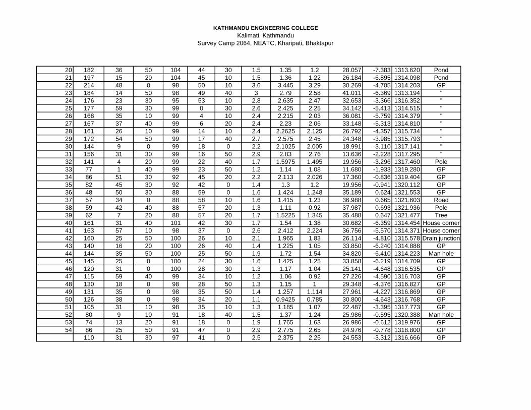
KATHMANDU ENGINEERING COLLEGE Kalimati, Kathmandu
Survey Camp 2064, NEATC, Kharipati, Bhaktapur
20 182 36 50 104 44 30 1.5 1.35 1.2 28.057 -7.383 1313.620 Pond21 197 15 20 104 45 10 1.5 1.36 1.22 26.184 -6.895 1314.098 Pond22 214 48 0 98 50 10 3.6 3.445 3.29 30.269 -4.705 1314.203 GP23 184 14 50 98 49 40 3 2.79 2.58 41.011 -6.369 1313.194 "24 176 23 30 95 53 10 2.8 2.635 2.47 32.653 -3.366 1316.352 "25 177 59 30 99 0 30 2.6 2.425 2.25 34.142 -5.413 1314.515 "26 168 35 10 99 4 10 2.4 2.215 2.03 36.081 -5.759 1314.379 "27 167 37 40 99 6 20 2.4 2.23 2.06 33.148 -5.313 1314.810 "28 161 26 10 99 14 10 2.4 2.2625 2.125 26.792 -4.357 1315.734 "29 172 54 50 99 17 40 2.7 2.575 2.45 24.348 -3.985 1315.793 "30 144 9 0 99 18 0 2.2 2.1025 2.005 18.991 -3.110 1317.141 "31 156 31 30 99 16 50 2.9 2.83 2.76 13.636 -2.228 1317.295 "32 141 4 20 99 22 40 1.7 1.5975 1.495 19.956 -3.296 1317.460 Pole33 77 1 40 99 23 50 1.2 1.14 1.08 11.680 -1.933 1319.280 GP34 86 51 30 92 45 20 2.2 2.113 2.026 17.360 -0.836 1319.404 GP35 82 45 30 92 42 0 1.4 1.3 1.2 19.956 -0.941 1320.112 GP36 48 50 30 88 59 0 1.6 1.424 1.248 35.189 0.624 1321.553 GP37 57 34 0 88 58 10 1.6 1.415 1.23 36.988 0.665 1321.603 Road38 59 42 40 88 57 20 1.3 1.11 0.92 37.987 0.693 1321.936 Pole39 62 7 20 88 57 20 1.7 1.5225 1.345 35.488 0.647 1321.477 Tree40 161 31 40 101 42 30 1.7 1.54 1.38 30.682 -6.359 1314.454 House corner41 163 57 10 98 37 0 2.6 2.412 2.224 36.756 -5.570 1314.371 House corner42 160 25 50 100 26 10 2.1 1.965 1.83 26.114 -4.810 1315.578 Drain junction43 140 16 20 100 26 40 1.4 1.225 1.05 33.850 -6.240 1314.888 GP44 144 35 50 100 25 50 1.9 1.72 1.54 34.820 -6.410 1314.223 Man hole45 145 25 0 100 24 30 1.6 1.425 1.25 33.858 -6.219 1314.709 GP46 120 31 0 100 28 30 1.3 1.17 1.04 25.141 -4.648 1316.535 GP47 115 59 40 99 34 10 1.2 1.06 0.92 27.226 -4.590 1316.703 GP48 130 18 0 98 28 50 1.3 1.15 1 29.348 -4.376 1316.827 GP49 131 35 0 98 35 50 1.4 1.257 1.114 27.961 -4.227 1316.869 GP50 126 38 0 98 34 20 1.1 0.9425 0.785 30.800 -4.643 1316.768 GP51 105 31 10 98 35 10 1.3 1.185 1.07 22.487 -3.395 1317.773 GP52 80 9 10 91 18 40 1.5 1.37 1.24 25.986 -0.595 1320.388 Man hole53 74 13 20 91 18 0 1.9 1.765 1.63 26.986 -0.612 1319.976 GP54 86 25 50 91 47 0 2.9 2.775 2.65 24.976 -0.778 1318.800 GP
110 31 30 97 41 0 2.5 2.375 2.25 24.553 -3.312 1316.666 GP
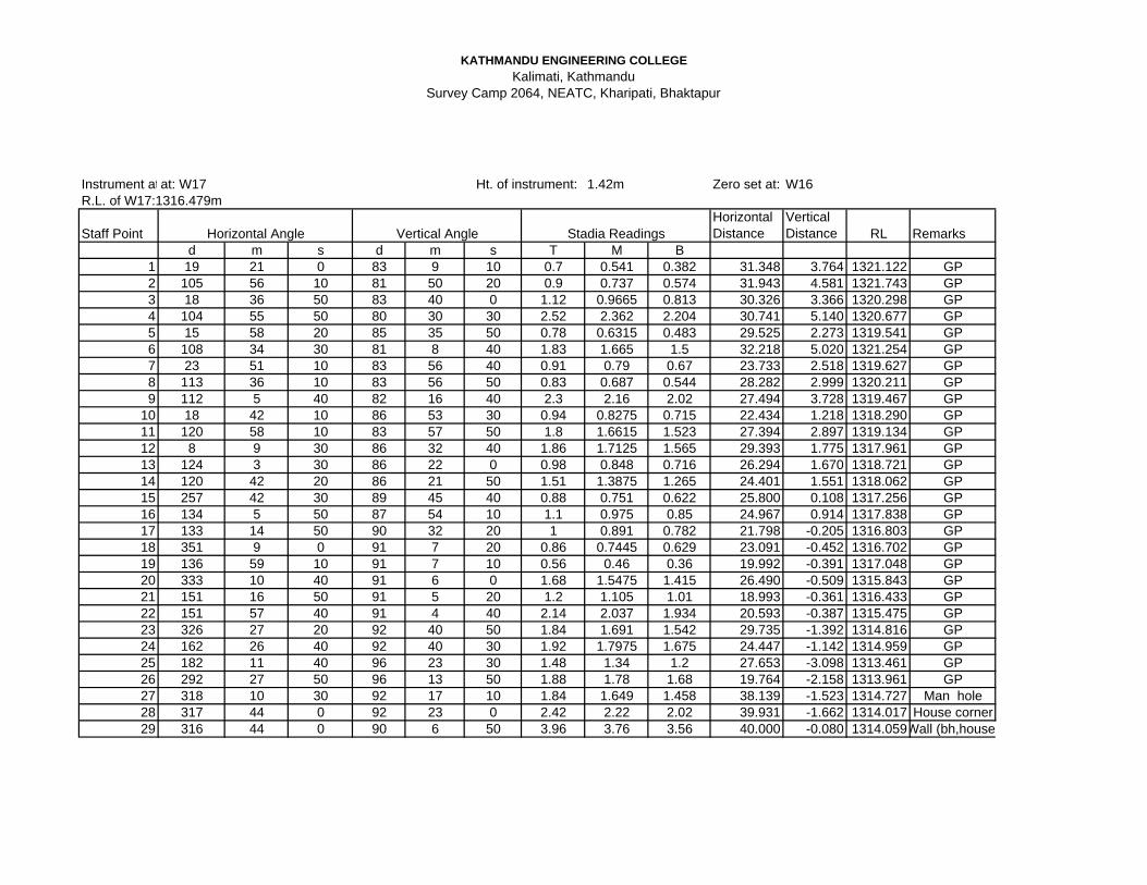
KATHMANDU ENGINEERING COLLEGE Kalimati, Kathmandu
Survey Camp 2064, NEATC, Kharipati, Bhaktapur
Instrument atat: W17 1.42m Zero set at: W16R.L. of W17:1316.479m
Staff PointHorizontal Distance
Vertical Distance RL Remarks
d m s d m s T M B1 19 21 0 83 9 10 0.7 0.541 0.382 31.348 3.764 1321.122 GP2 105 56 10 81 50 20 0.9 0.737 0.574 31.943 4.581 1321.743 GP3 18 36 50 83 40 0 1.12 0.9665 0.813 30.326 3.366 1320.298 GP4 104 55 50 80 30 30 2.52 2.362 2.204 30.741 5.140 1320.677 GP5 15 58 20 85 35 50 0.78 0.6315 0.483 29.525 2.273 1319.541 GP6 108 34 30 81 8 40 1.83 1.665 1.5 32.218 5.020 1321.254 GP7 23 51 10 83 56 40 0.91 0.79 0.67 23.733 2.518 1319.627 GP8 113 36 10 83 56 50 0.83 0.687 0.544 28.282 2.999 1320.211 GP9 112 5 40 82 16 40 2.3 2.16 2.02 27.494 3.728 1319.467 GP
10 18 42 10 86 53 30 0.94 0.8275 0.715 22.434 1.218 1318.290 GP11 120 58 10 83 57 50 1.8 1.6615 1.523 27.394 2.897 1319.134 GP12 8 9 30 86 32 40 1.86 1.7125 1.565 29.393 1.775 1317.961 GP13 124 3 30 86 22 0 0.98 0.848 0.716 26.294 1.670 1318.721 GP14 120 42 20 86 21 50 1.51 1.3875 1.265 24.401 1.551 1318.062 GP15 257 42 30 89 45 40 0.88 0.751 0.622 25.800 0.108 1317.256 GP16 134 5 50 87 54 10 1.1 0.975 0.85 24.967 0.914 1317.838 GP17 133 14 50 90 32 20 1 0.891 0.782 21.798 -0.205 1316.803 GP18 351 9 0 91 7 20 0.86 0.7445 0.629 23.091 -0.452 1316.702 GP19 136 59 10 91 7 10 0.56 0.46 0.36 19.992 -0.391 1317.048 GP20 333 10 40 91 6 0 1.68 1.5475 1.415 26.490 -0.509 1315.843 GP21 151 16 50 91 5 20 1.2 1.105 1.01 18.993 -0.361 1316.433 GP22 151 57 40 91 4 40 2.14 2.037 1.934 20.593 -0.387 1315.475 GP23 326 27 20 92 40 50 1.84 1.691 1.542 29.735 -1.392 1314.816 GP24 162 26 40 92 40 30 1.92 1.7975 1.675 24.447 -1.142 1314.959 GP25 182 11 40 96 23 30 1.48 1.34 1.2 27.653 -3.098 1313.461 GP26 292 27 50 96 13 50 1.88 1.78 1.68 19.764 -2.158 1313.961 GP27 318 10 30 92 17 10 1.84 1.649 1.458 38.139 -1.523 1314.727 Man hole28 317 44 0 92 23 0 2.42 2.22 2.02 39.931 -1.662 1314.017 House corner29 316 44 0 90 6 50 3.96 3.76 3.56 40.000 -0.080 1314.059Wall (bh,house
Ht. of instrument:
Horizontal Angle Vertical Angle Stadia Readings

KATHMANDU ENGINEERING COLLEGE Kalimati, Kathmandu
Survey Camp 2064, NEATC, Kharipati, Bhaktapur
Instrument atat: W18 1.4m Zero set at: W17R.L. of W18:1326.057m
Staff PointHorizontal Distance
Vertical Distance RL Remarks
d m s d m s T M B1 193 11 40 87 21 0 1 0.8075 0.615 38.418 1.778 1328.4282 203 40 30 87 31 40 2.3 2.095 1.89 40.924 1.767 1327.1293 214 13 20 87 35 40 2.455 2.3175 2.18 27.452 1.153 1326.2934 230 53 50 91 42 50 2.361 2.273 2.185 17.584 -0.526 1324.6585 242 42 10 91 42 30 2.495 2.404 2.313 18.184 -0.542 1324.5116 17 17 0 91 42 30 1.923 1.81 1.697 22.580 -0.673 1324.9747 28 48 50 91 40 50 2.895 2.675 2.455 43.962 -1.290 1323.4928 28 46 40 91 40 10 1.642 1.5585 1.475 16.686 -0.486 1325.4129 34 20 10 91 40 10 2.535 2.335 2.135 39.966 -1.165 1323.957
10 48 7 30 91 41 0 2.202 2.053 1.904 29.774 -0.875 1324.52911 37 16 40 91 10 20 1.3 1.255 1.21 8.996 -0.184 1326.01812 51 45 0 91 9 30 1.753 1.579 1.405 34.786 -0.703 1325.17513 65 17 10 90 44 10 1.3 1.2225 1.145 15.497 -0.199 1326.03514 86 11 40 90 44 30 1.4 1.2585 1.117 28.295 -0.366 1325.83215 110 4 50 90 44 30 0.97 0.825 0.68 28.995 -0.375 1326.25716 131 19 50 84 21 20 1.3 1.1325 0.965 33.176 3.279 1329.60317 166 7 30 89 3 0 1.1 0.99 0.88 21.994 0.365 1326.83218 153 3 40 82 22 30 2.3 2.135 1.97 32.419 4.340 1329.66219 153 40 10 82 27 10 2 1.8475 1.695 29.974 3.971 1329.58120 168 23 40 82 23 30 2.3 2.1375 1.975 31.930 4.265 1329.58521 185 7 40 83 34 0 2.1 1.91 1.72 37.523 4.231 1329.77822 184 1 0 83 23 30 2.6 2.4 2.2 39.470 4.573 1329.63023 184 25 40 83 30 20 1.9 1.7165 1.533 36.230 4.124 1329.86524 186 34 30 84 31 30 1.5 1.325 1.15 34.681 3.324 1329.45625 193 40 40 86 33 20 2 1.805 1.61 38.859 2.339 1327.99126 99 26 20 88 52 50 2 1.81 1.62 37.985 0.742 1326.38927 206 50 40 87 27 40 1.8 1.6425 1.485 31.438 1.394 1327.20928 200 25 20 88 15 50 1.9 1.655 1.41 48.955 1.484 1327.286
Ht. of instrument:
Horizontal Angle Vertical Angle Stadia Readings

KATHMANDU ENGINEERING COLLEGE Kalimati, Kathmandu
Survey Camp 2064, NEATC, Kharipati, Bhaktapur
Instrument atat: W19 1.47m Zero set at: W18R.L. of W19:1328.977m
Staff PointHorizontal Distance
Vertical Distance RL Remarks
d m s d m s T M B1 291 18 20 95 21 50 1.93 1.9085 1.887 4.262 -0.400 1328.1382 229 51 50 95 20 0 1.388 1.381 1.374 1.388 -0.130 1328.9363 219 37 30 95 32 30 1.4 1.3535 1.307 9.213 -0.894 1328.2004 217 41 50 91 18 10 1.98 1.9055 1.831 14.892 -0.339 1328.2035 199 38 10 89 20 50 2.4 2.3125 2.225 17.498 0.199 1328.3346 198 51 30 90 17 0 1.76 1.6865 1.613 14.700 -0.073 1328.6887 201 57 20 90 11 40 1.86 1.8285 1.797 6.300 -0.021 1328.5978 36 26 20 89 14 50 1.3 1.2075 1.115 18.497 0.243 1329.4839 38 49 20 85 22 30 1.7 1.5905 1.481 21.758 1.760 1330.617
10 15 44 0 85 20 20 2.2 2.57 2.94 -73.511 -5.994 1321.88311 31 43 10 85 13 10 2.2 2.57 2.94 -73.486 -6.146 1321.73112 33 8 50 85 45 20 2.2 2.05 1.9 29.836 2.214 1330.61113 42 11 40 84 50 20 2.2 2.05 1.9 29.757 2.688 1331.08514 43 21 50 86 6 0 2.2 2.0075 1.815 38.322 2.613 1331.05215 52 47 0 85 26 0 3.1 2.8815 2.663 43.423 3.468 1331.03416 53 10 30 85 25 10 1.9 1.6825 1.465 43.223 3.463 1332.22717 54 35 30 83 43 40 2.7 2.5 2.3 39.523 4.344 1332.29118 65 46 20 85 33 10 2.5 2.3285 2.157 34.094 2.652 1330.77019 72 4 50 79 10 20 2.5 2.364 2.228 26.240 5.019 1333.10220 79 31 10 82 4 20 1.9 1.8475 1.795 10.300 1.434 1330.03421 98 22 40 77 0 0 1.7 1.6025 1.505 18.513 4.274 1333.11922 107 25 50 78 29 0 2.5 2.371 2.242 24.772 5.047 1333.12323 99 32 10 76 37 10 1.5 1.41 1.32 17.036 4.052 1333.08924 92 39 0 76 5 50 1.6 1.51 1.42 16.961 4.198 1333.13525 80 51 20 85 15 10 1.03 0.965 0.9 12.911 1.072 1330.55426 64 52 50 83 12 30 1.5 1.3975 1.295 20.213 2.407 1331.45727 47 41 10 90 12 0 0.9 0.805 0.71 19.000 -0.066 1329.57628 162 27 50 90 8 50 1.25 1.215 1.18 7.000 -0.018 1329.21429 180 15 50 90 10 10 1.96 1.9275 1.895 6.500 -0.019 1328.50030 194 36 40 90 33 10 1.08 0.97 0.86 21.998 -0.212 1329.265
Horizontal Angle Vertical Angle Stadia Readings
Ht. of instrument:
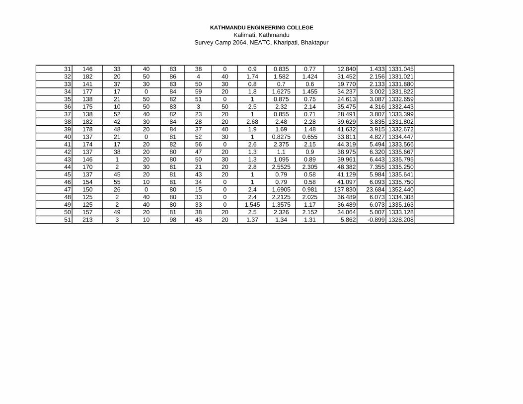
KATHMANDU ENGINEERING COLLEGE Kalimati, Kathmandu
Survey Camp 2064, NEATC, Kharipati, Bhaktapur
31 146 33 40 83 38 0 0.9 0.835 0.77 12.840 1.433 1331.04532 182 20 50 86 4 40 1.74 1.582 1.424 31.452 2.156 1331.02133 141 37 30 83 50 30 0.8 0.7 0.6 19.770 2.133 1331.88034 177 17 0 84 59 20 1.8 1.6275 1.455 34.237 3.002 1331.82235 138 21 50 82 51 0 1 0.875 0.75 24.613 3.087 1332.65936 175 10 50 83 3 50 2.5 2.32 2.14 35.475 4.316 1332.44337 138 52 40 82 23 20 1 0.855 0.71 28.491 3.807 1333.39938 182 42 30 84 28 20 2.68 2.48 2.28 39.629 3.835 1331.80239 178 48 20 84 37 40 1.9 1.69 1.48 41.632 3.915 1332.67240 137 21 0 81 52 30 1 0.8275 0.655 33.811 4.827 1334.44741 174 17 20 82 56 0 2.6 2.375 2.15 44.319 5.494 1333.56642 137 38 20 80 47 20 1.3 1.1 0.9 38.975 6.320 1335.66743 146 1 20 80 50 30 1.3 1.095 0.89 39.961 6.443 1335.79544 170 2 30 81 21 20 2.8 2.5525 2.305 48.382 7.355 1335.25045 137 45 20 81 43 20 1 0.79 0.58 41.129 5.984 1335.64146 154 55 10 81 34 0 1 0.79 0.58 41.097 6.093 1335.75047 150 26 0 80 15 0 2.4 1.6905 0.981 137.830 23.684 1352.44048 125 2 40 80 33 0 2.4 2.2125 2.025 36.489 6.073 1334.30849 125 2 40 80 33 0 1.545 1.3575 1.17 36.489 6.073 1335.16350 157 49 20 81 38 20 2.5 2.326 2.152 34.064 5.007 1333.12851 213 3 10 98 43 20 1.37 1.34 1.31 5.862 -0.899 1328.208

KATHMANDU ENGINEERING COLLEGE Kalimati, Kathmandu
Survey Camp 2064, NEATC, Kharipati, Bhaktapur
er

KATHMANDU ENGINEERING COLLEGE Kalimati, Kathmandu
Survey Camp 2064, NEATC, Kharipati, Bhaktapur
t
er

KATHMANDU ENGINEERING COLLEGE Kalimati, Kathmandu
Survey Camp 2064, NEATC, Kharipati, Bhaktapur

KATHMANDU ENGINEERING COLLEGE Kalimati, Kathmandu
Survey Camp 2064, NEATC, Kharipati, Bhaktapur

KATHMANDU ENGINEERING COLLEGE Kalimati, Kathmandu
Survey Camp 2064, NEATC, Kharipati, Bhaktapur
r

KATHMANDU ENGINEERING COLLEGE Kalimati, Kathmandu
Survey Camp 2064, NEATC, Kharipati, Bhaktapur

KATHMANDU ENGINEERING COLLEGE Kalimati, Kathmandu
Survey Camp 2064, NEATC, Kharipati, Bhaktapur
rr

KATHMANDU ENGINEERING COLLEGE Kalimati, Kathmandu
Survey Camp 2064, NEATC, Kharipati, Bhaktapur

KATHMANDU ENGINEERING COLLEGE Kalimati, Kathmandu
Survey Camp 2064, NEATC, Kharipati, Bhaktapur

KATHMANDU ENGINEERING COLLEGE Kalimati, Kathmandu
Survey Camp 2064, NEATC, Kharipati, Bhaktapur

KATHMANDU ENGINEERING COLLEGE Kalimati, Kathmandu
Survey Camp 2064, NEATC, Kharipati, Bhaktapur

KATHMANDU ENGINEERING COLLEGE Kalimati, Kathmandu
Survey Camp 2064, NEATC, Kharipati, Bhaktapur

KATHMANDU ENGINEERING COLLEGE Kalimati, Kathmandu
Survey Camp 2064, NEATC, Kharipati, Bhaktapur

KATHMANDU ENGINEERING COLLEGE Kalimati, Kathmandu
Survey Camp 2064, NEATC, Kharipati, Bhaktapur

KATHMANDU ENGINEERING COLLEGE Kalimati, Kathmandu
Survey Camp 2064, NEATC, Kharipati, Bhaktapur

KATHMANDU ENGINEERING COLLEGE Kalimati, Kathmandu
Survey Camp 2064, NEATC, Kharipati, Bhaktapur

KATHMANDU ENGINEERING COLLEGE Kalimati, Kathmandu
Survey Camp 2064, NEATC, Kharipati, Bhaktapur

KATHMANDU ENGINEERING COLLEGE Kalimati, Kathmandu
Survey Camp 2064, NEATC, Kharipati, Bhaktapur
)
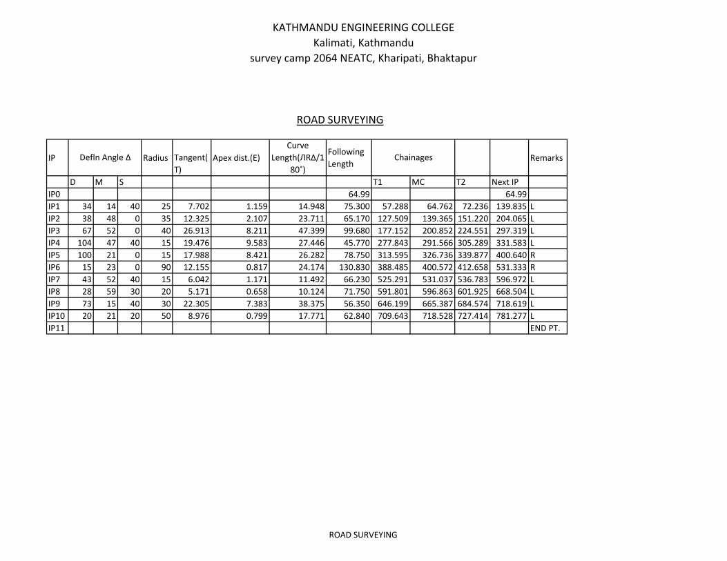
KATHMANDU ENGINEERING COLLEGEKalimati, Kathmandu
survey camp 2064 NEATC, Kharipati, Bhaktapur
IP Radius Tangent(T)
Apex dist.(E)Curve
Length(ЛR∆/180˚)
Following Length
Remarks
D M S T1 MC T2 Next IPIP0 64.99 64.99IP1 34 14 40 25 7.702 1.159 14.948 75.300 57.288 64.762 72.236 139.835 LIP2 38 48 0 35 12.325 2.107 23.711 65.170 127.509 139.365 151.220 204.065 LIP3 67 52 0 40 26.913 8.211 47.399 99.680 177.152 200.852 224.551 297.319 LIP4 104 47 40 15 19.476 9.583 27.446 45.770 277.843 291.566 305.289 331.583 LIP5 100 21 0 15 17.988 8.421 26.282 78.750 313.595 326.736 339.877 400.640 RIP6 15 23 0 90 12.155 0.817 24.174 130.830 388.485 400.572 412.658 531.333 RIP7 43 52 40 15 6.042 1.171 11.492 66.230 525.291 531.037 536.783 596.972 LIP8 28 59 30 20 5.171 0.658 10.124 71.750 591.801 596.863 601.925 668.504 LIP9 73 15 40 30 22.305 7.383 38.375 56.350 646.199 665.387 684.574 718.619 LIP10 20 21 20 50 8.976 0.799 17.771 62.840 709.643 718.528 727.414 781.277 LIP11 END PT.
ROAD SURVEYING
Defln Angle ∆ Chainages
ROAD SURVEYING
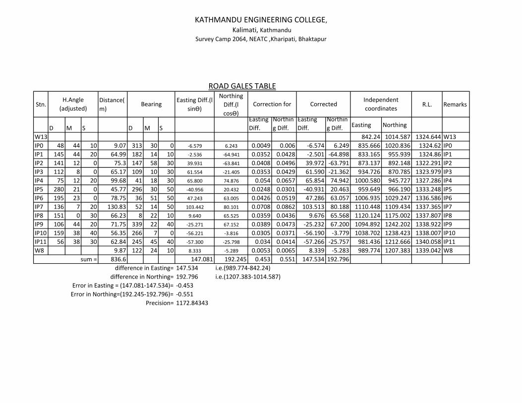
KATHMANDU ENGINEERING COLLEGE, Kalimati, Kathmandu
Survey Camp 2064, NEATC ,Kharipati, Bhaktapur
Stn.Distance(m)
Easting Diff.(l sinѲ)
Northing Diff.(l cosѲ)
R.L. Remarks
D M S D M SEasting Diff.
Northing Diff.
Easting Diff.
Northing Diff. Easting Northing
W13 842.24 1014.587 1324.644 W13IP0 48 44 10 9.07 313 30 0 ‐6.579 6.243 0.0049 0.006 ‐6.574 6.249 835.666 1020.836 1324.62 IP0IP1 145 44 20 64.99 182 14 10 ‐2.536 ‐64.941 0.0352 0.0428 ‐2.501 ‐64.898 833.165 955.939 1324.86 IP1IP2 141 12 0 75.3 147 58 30 39.931 ‐63.841 0.0408 0.0496 39.972 ‐63.791 873.137 892.148 1322.291 IP2IP3 112 8 0 65.17 109 10 30 61.554 ‐21.405 0.0353 0.0429 61.590 ‐21.362 934.726 870.785 1323.979 IP3IP4 75 12 20 99.68 41 18 30 65.800 74.876 0.054 0.0657 65.854 74.942 1000.580 945.727 1327.286 IP4IP5 280 21 0 45.77 296 30 50 ‐40.956 20.432 0.0248 0.0301 ‐40.931 20.463 959.649 966.190 1333.248 IP5IP6 195 23 0 78.75 36 51 50 47.243 63.005 0.0426 0.0519 47.286 63.057 1006.935 1029.247 1336.586 IP6IP7 136 7 20 130.83 52 14 50 103.442 80.101 0.0708 0.0862 103.513 80.188 1110.448 1109.434 1337.365 IP7IP8 151 0 30 66.23 8 22 10 9.640 65.525 0.0359 0.0436 9.676 65.568 1120.124 1175.002 1337.807 IP8IP9 106 44 20 71.75 339 22 40 ‐25.271 67.152 0.0389 0.0473 ‐25.232 67.200 1094.892 1242.202 1338.922 IP9IP10 159 38 40 56.35 266 7 0 ‐56.221 ‐3.816 0.0305 0.0371 ‐56.190 ‐3.779 1038.702 1238.423 1338.007 IP10IP11 56 38 30 62.84 245 45 40 ‐57.300 ‐25.798 0.034 0.0414 ‐57.266 ‐25.757 981.436 1212.666 1340.058 IP11W8 9.87 122 24 10 8.333 ‐5.289 0.0053 0.0065 8.339 ‐5.283 989.774 1207.383 1339.042 W8
836.6 147.081 192.245 0.453 0.551 147.534 192.796147.534 i.e.(989.774‐842.24)192.796 i.e.(1207.383‐1014.587)‐0.453‐0.5511172.84343
Independent coordinates
Precision=
ROAD GALES TABLE
Error in Easting = (147.081‐147.534)=Error in Northing=(192.245‐192.796)=
difference in Northing=difference in Easting=
sum =
BearingH.Angle (adjusted)
Correction for Corrected

KATHMANDU ENGINEERING COLLEGEKalimati, Kathmandu
Survey Camp 2064, NEATC, Kharipati, Bhaktapur
Road Survey Detailing
Zero set at:W13 R.L. OF IP0:1324.620MInst.Stn./HI. Staff Point
Horizantal distance
Vertical distance R.L. Remarks
d m s d m s Top middle BottomIP0/1.40 W13 0 0 0 1324.644 w13
IP1 48 44 10 89 39 20 1.9 1.575 1.250 64.998 0.391 1324.8360+00 5R 128 34 40 96 54 10 2.7 2.675 2.650 4.928 ‐0.597 1322.748
8R 125 25 50 98 44 50 2 1.940 1.880 11.722 ‐1.804 1322.276POND 125 25 40 103 40 20 2 1.938 1.875 11.802 ‐2.871 1321.212 POND 2M RADIS
WALL R10M 125 16 0 98 1 0 1.8 1.710 1.620 17.650 ‐2.486 1321.824 WALL BOUNDARY
3ML 308 44 0 93 53 40 1.2 1.180 1.160 3.982 ‐0.271 1324.5699ML 307 6 40 93 40 0 1.6 1.560 1.520 7.967 ‐0.511 1323.94910ML 308 49 40 91 39 10 1 0.926 0.852 14.788 ‐0.427 1324.6670+020 48 38 0 95 59 40 1.7 1.600 1.500 19.782 ‐2.077 1322.3436L 29 47 40 94 34 10 1 0.895 0.790 20.867 ‐1.668 1323.4577L 22 14 30 90 5 30 1.4 1.295 1.190 21.000 ‐0.034 1324.69113L 12 8 20 90 18 0 1.3 1.190 1.080 21.999 ‐0.115 1324.7155R 62 29 0 97 32 100 1.8 1.690 1.580 21.619 ‐2.870 1321.46010R 72 40 0 97 29 40 1.6 1.480 1.360 23.592 ‐3.104 1321.436POLE RODE 25 45 40 91 54 40 1 0.925 0.850 14.983 ‐0.500 1324.595P2 182 13 10 92 56 20 1.28 1.260 1.240 3.989 ‐0.205 1324.5550+40 48 49 20 93 14 10 1.2 1.000 0.800 39.873 ‐2.254 1322.7661MR 50 15 0 93 17 20 1.6 1.400 1.200 39.868 ‐2.291 1322.3295MR 56 47 30 94 28 0 1.4 1.200 1.000 39.757 ‐3.106 1321.7148R 60 36 40 95 53 40 1.2 1.000 0.800 39.578 ‐4.086 1320.93410R 65 28 30 95 50 50 1.2 1.000 0.800 39.585 ‐4.054 1320.96611R 65 24 30 95 50 50 1.2 1.000 0.800 39.585 ‐4.054 1320.9665L 39 30 30 92 21 40 1.2 1.000 0.800 39.932 ‐1.647 1323.37310L 32 13 30 90 25 50 1.2 0.980 0.760 43.998 ‐0.331 1324.709RP3 24 51 20 90 31 0 0.8 0.400 0.000 79.993 ‐0.721 1324.899
Stadia ReadingsHorizontal Angle Vertical Angle
Road Survey Gropu J
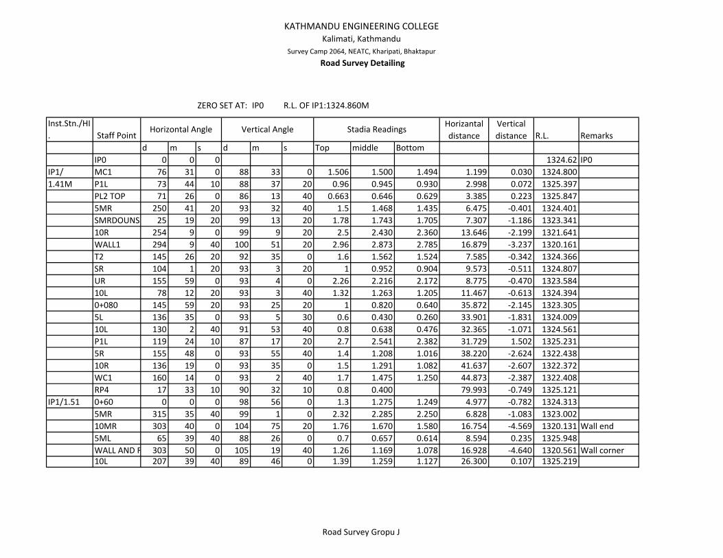
KATHMANDU ENGINEERING COLLEGEKalimati, Kathmandu
Survey Camp 2064, NEATC, Kharipati, Bhaktapur
Road Survey Detailing
ZERO SET AT: IP0 R.L. OF IP1:1324.860M
Inst.Stn./HI. Staff Point
Horizantal distance
Vertical distance R.L. Remarks
d m s d m s Top middle BottomIP0 0 0 0 1324.62 IP0
IP1/ MC1 76 31 0 88 33 0 1.506 1.500 1.494 1.199 0.030 1324.8001.41M P1L 73 44 10 88 37 20 0.96 0.945 0.930 2.998 0.072 1325.397
PL2 TOP 71 26 0 86 13 40 0.663 0.646 0.629 3.385 0.223 1325.8475MR 250 41 20 93 32 40 1.5 1.468 1.435 6.475 ‐0.401 1324.401SMRDOUNS 25 19 20 99 13 20 1.78 1.743 1.705 7.307 ‐1.186 1323.34110R 254 9 0 99 9 20 2.5 2.430 2.360 13.646 ‐2.199 1321.641WALL1 294 9 40 100 51 20 2.96 2.873 2.785 16.879 ‐3.237 1320.161T2 145 26 20 92 35 0 1.6 1.562 1.524 7.585 ‐0.342 1324.366SR 104 1 20 93 3 20 1 0.952 0.904 9.573 ‐0.511 1324.807UR 155 59 0 93 4 0 2.26 2.216 2.172 8.775 ‐0.470 1323.58410L 78 12 20 93 3 40 1.32 1.263 1.205 11.467 ‐0.613 1324.3940+080 145 59 20 93 25 20 1 0.820 0.640 35.872 ‐2.145 1323.3055L 136 35 0 93 5 30 0.6 0.430 0.260 33.901 ‐1.831 1324.00910L 130 2 40 91 53 40 0.8 0.638 0.476 32.365 ‐1.071 1324.561P1L 119 24 10 87 17 20 2.7 2.541 2.382 31.729 1.502 1325.2315R 155 48 0 93 55 40 1.4 1.208 1.016 38.220 ‐2.624 1322.43810R 136 19 0 93 35 0 1.5 1.291 1.082 41.637 ‐2.607 1322.372WC1 160 14 0 93 2 40 1.7 1.475 1.250 44.873 ‐2.387 1322.408RP4 17 33 10 90 32 10 0.8 0.400 79.993 ‐0.749 1325.121
IP1/1.51 0+60 0 0 0 98 56 0 1.3 1.275 1.249 4.977 ‐0.782 1324.3135MR 315 35 40 99 1 0 2.32 2.285 2.250 6.828 ‐1.083 1323.00210MR 303 40 0 104 75 20 1.76 1.670 1.580 16.754 ‐4.569 1320.131 Wall end5ML 65 39 40 88 26 0 0.7 0.657 0.614 8.594 0.235 1325.948WALL AND R 303 50 0 105 19 40 1.26 1.169 1.078 16.928 ‐4.640 1320.561 Wall corner10L 207 39 40 89 46 0 1.39 1.259 1.127 26.300 0.107 1325.219
Horizontal Angle Vertical Angle Stadia Readings
Road Survey Gropu J
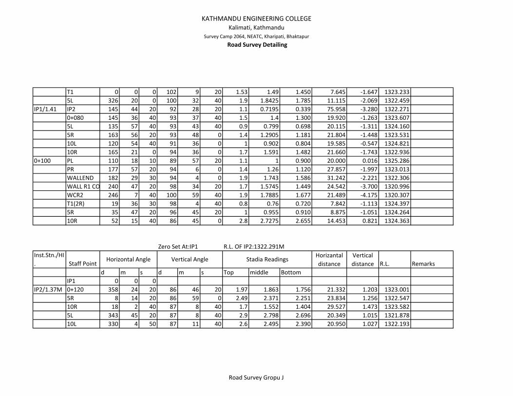
KATHMANDU ENGINEERING COLLEGEKalimati, Kathmandu
Survey Camp 2064, NEATC, Kharipati, Bhaktapur
Road Survey Detailing
T1 0 0 0 102 9 20 1.53 1.49 1.450 7.645 ‐1.647 1323.2335L 326 20 0 100 32 40 1.9 1.8425 1.785 11.115 ‐2.069 1322.459
IP1/1.41 IP2 145 44 20 92 28 20 1.1 0.7195 0.339 75.958 ‐3.280 1322.2710+080 145 36 40 93 37 40 1.5 1.4 1.300 19.920 ‐1.263 1323.6075L 135 57 40 93 43 40 0.9 0.799 0.698 20.115 ‐1.311 1324.1605R 163 56 20 93 48 0 1.4 1.2905 1.181 21.804 ‐1.448 1323.53110L 120 54 40 91 36 0 1 0.902 0.804 19.585 ‐0.547 1324.82110R 165 21 0 94 36 0 1.7 1.591 1.482 21.660 ‐1.743 1322.936
0+100 PL 110 18 10 89 57 20 1.1 1 0.900 20.000 0.016 1325.286PR 177 57 20 94 6 0 1.4 1.26 1.120 27.857 ‐1.997 1323.013WALLEND 182 29 30 94 4 0 1.9 1.743 1.586 31.242 ‐2.221 1322.306WALL R1 CO 240 47 20 98 34 20 1.7 1.5745 1.449 24.542 ‐3.700 1320.996WCR2 246 7 40 100 59 40 1.9 1.7885 1.677 21.489 ‐4.175 1320.307T1(2R) 19 36 30 98 4 40 0.8 0.76 0.720 7.842 ‐1.113 1324.3975R 35 47 20 96 45 20 1 0.955 0.910 8.875 ‐1.051 1324.26410R 52 15 40 86 45 0 2.8 2.7275 2.655 14.453 0.821 1324.363
Zero Set At:IP1 R.L. OF IP2:1322.291MInst.Stn./HI. Staff Point
Horizantal distance
Vertical distance R.L. Remarks
d m s d m s Top middle BottomIP1 0 0 0
IP2/1.37M 0+120 358 24 20 86 46 20 1.97 1.863 1.756 21.332 1.203 1323.0015R 8 14 20 86 59 0 2.49 2.371 2.251 23.834 1.256 1322.54710R 18 2 40 87 8 40 1.7 1.552 1.404 29.527 1.473 1323.5825L 343 45 20 87 8 40 2.9 2.798 2.696 20.349 1.015 1321.87810L 330 4 50 87 11 40 2.6 2.495 2.390 20.950 1.027 1322.193
Horizontal Angle Vertical Angle Stadia Readings
Road Survey Gropu J

KATHMANDU ENGINEERING COLLEGEKalimati, Kathmandu
Survey Camp 2064, NEATC, Kharipati, Bhaktapur
Road Survey Detailing
PL 314 5 0 89 39 20 2.8 2.695 2.590 20.999 0.126 1321.092127.502 T1 0 14 20 92 40 45 0.4 0.338 0.275 12.473 ‐0.584 1322.740
L5 19 59 0 91 15 40 0.9 0.831 0.762 13.793 ‐0.304 1322.526R10 36 25 0 88 15 20 1.5 1.410 1.319 18.083 0.551 1322.802R5 324 55 20 89 15 40 2 1.907 1.814 18.597 0.240 1321.994R10 301 1 40 94 21 40 1.34 1.257 1.174 16.504 ‐1.259 1321.145T2 141 15 20 89 36 0 1.5 1.438 1.375 12.499 0.087 1322.311R5 122 10 20 88 16 40 0.89 0.805 0.720 16.985 0.511 1323.367L10 109 39 40 86 44 0 1.77 1.653 1.535 23.424 1.337 1323.345R5 170 57 0 92 57 20 1.3 1.150 1.000 29.920 ‐1.545 1320.966R10 217 5 0 93 0 0 1.6 1.397 1.194 40.489 ‐2.122 1320.142P1 71 1 50 93 37 0 1.5 1.480 1.460 3.984 ‐0.252 1321.929
139.353 MC 70 10 40 91 51 20 1.8 1.788 1.776 2.397 ‐0.078 1321.795R5 251 13 0 96 16 40 1.5 1.483 1.465 3.458 ‐0.380 1321.798R10 250 57 10 96 13 40 0.8 0.740 0.680 11.859 ‐1.294 1321.627L5 70 34 30 96 13 0 0.6 0.568 0.535 6.424 ‐0.700 1322.394L10 73 22 40 85 22 50 1.7 1.623 1.545 15.399 1.244 1323.2830+160 141 53 20 87 10 30 1.5 1.445 1.390 10.973 0.541 1322.757L5 125 49 20 87 11 0 1.4 1.290 1.180 21.947 1.080 1323.451L10 108 5 40 87 5 20 1 0.868 0.735 26.432 1.344 1324.138R5 160 35 0 87 10 30 1.9 1.790 1.680 21.947 1.083 1322.954R10 175 45 50 90 45 50 1 0.875 0.750 24.996 ‐0.333 1322.453ROAD1 125 54 40 87 38 40 1 0.820 0.640 35.939 1.478 1324.319P1 119 58 30 87 38 40 1 0.820 0.640 35.939 1.478 1324.319P2 153 46 50 89 34 0 1 0.840 0.680 31.998 0.242 1323.063R2 155 55 30 89 29 10 1.4 1.273 1.145 25.498 0.229 1322.617
Road Survey Gropu J

KATHMANDU ENGINEERING COLLEGEKalimati, Kathmandu
Survey Camp 2064, NEATC, Kharipati, Bhaktapur
Road Survey Detailing
Zero Set At:IP2 R.L.OF IP3:1323.979MInst.Stn./HI. Staff Point
Horizantal distance
Vertical distance R.L. Remarks
d m s d m s Top middle BottomIP2 0 0 0 92 6 20 1 0.670 0.340 65.911 ‐2.423 1322.276
IP3/1.39 0+180 359 35 20 92 53 20 0.8 0.677 0.554 24.538 ‐1.238 1323.454 T1L5 7 3 20 92 52 0 0.5 0.376 0.252 24.738 ‐1.239 1323.754L10 28 40 20 91 51 0 0.7 0.565 0.430 26.972 ‐0.871 1323.933R5 342 25 20 91 40 40 1.8 1.666 1.532 26.777 ‐0.784 1322.919R10 323 36 20 92 54 0 1.6 1.440 1.280 31.918 ‐1.617 1322.312IP4 110 5 0 88 4 40 2 1.500 1.000 99.887 3.352 1327.221MC(0+200) 55 4 0 88 5 0 1.92 1.879 1.838 8.191 0.274 1323.764L5 55 4 0 90 51 20 1.3 1.223 1.146 15.397 ‐0.230 1323.916L10 55 9 40 88 55 40 0.9 0.783 0.665 23.492 0.440 1325.026R5 241 17 40 97 33 10 1.25 1.244 1.238 1.179 ‐0.156 1323.969R10 237 50 40 92 6 20 1.8 1.753 1.706 9.387 ‐0.345 1323.271T2 110 30 40 94 11 0 1.6 1.466 1.332 26.657 ‐1.950 1321.953R5 125 24 0 88 18 20 1.6 1.465 1.330 26.976 0.798 1324.702R10 137 21 20 88 13 20 1.8 1.652 1.504 29.572 0.918 1324.635WALL 139 46 40 91 8 20 1.5 1.346 1.192 30.788 ‐0.612 1323.411R5 98 4 40 88 32 0 1.5 1.355 1.210 28.981 0.742 1324.756R10 90 39 20 83 54 20 1.7 1.525 1.350 34.605 3.695 1327.5390+240 110 13 40 87 36 0 1.8 1.595 1.390 40.928 1.715 1325.489R5 117 46 40 87 38 2 2 1.788 1.575 42.428 1.753 1325.335WALL END 122 4 40 87 38 2 2 1.788 1.575 42.428 1.753 1325.335L5 104 13 40 88 36 0 1.7 1.480 1.260 43.974 1.075 1324.964BC1 102 20 20 85 17 20 1.9 1.666 1.432 46.484 3.831 1327.534BC2 57 20 0 84 57 40 1 0.831 0.662 33.539 2.957 1327.495BC3 78 52 20 82 18 0 2.6 2.430 2.260 33.390 4.514 1327.453BC4 90 48 40 82 47 20 2.8 2.611 2.422 37.204 4.707 1327.465
Horizontal Angle Vertical Angle Stadia Readings
Road Survey Gropu J

KATHMANDU ENGINEERING COLLEGEKalimati, Kathmandu
Survey Camp 2064, NEATC, Kharipati, Bhaktapur
Road Survey Detailing
Zero Set At:IP3 R.L. OF IP4:1327.286MInst.Stn./HI. Staff Point
Horizantal distance
Vertical distance R.L. Remarks
d m s d m s Top middle BottomIP4/1.49 0+260 0 0 0 92 37 20 1.3 1.130 0.960 33.929 ‐1.554 1326.092
5R 356 46 0 92 33 20 1.9 1.702 1.504 39.521 ‐1.764 1325.310WALL C.(10R) 353 7 0 92 36 20 1.8 1.605 1.410 38.919 ‐1.771 1325.400
5L 6 42 20 92 56 20 1.1 0.948 0.795 30.420 ‐1.562 1326.2677L 12 57 40 92 43 40 1 0.783 0.565 43.401 ‐2.068 1325.926BC5 13 18 40 90 34 40 1 0.745 0.490 50.995 ‐0.514 1327.517IP5 75 12 0 82 53 0 1.5 1.265 1.030 46.279 5.778 1333.289
0+277 T1 359 49 20 95 39 20 1.3 1.202 1.104 19.410 ‐1.922 1325.652R5 348 49 20 95 41 40 1.6 1.496 1.391 20.694 ‐2.064 1325.217WC 343 29 0 95 46 0 1.4 1.290 1.180 21.778 ‐2.199 1325.287L5 13 33 40 92 17 20 1.6 1.540 1.480 11.981 ‐0.479 1326.757UP L5 20 32 20 88 58 0 1.2 1.124 1.048 15.195 0.274 1327.926L10 42 48 0 85 26 0 1.83 1.730 1.630 19.873 1.587 1328.633
0+291.53 MC 37 36 0 93 45 40 0.28 0.232 0.184 9.559 ‐0.628 1327.916R5 38 3 0 95 41 40 1.257 1.244 1.231 2.574 ‐0.257 1327.275L5 38 8 0 89 16 0 1 0.928 0.855 14.498 0.186 1328.034T2 75 56 20 82 28 40 1 0.902 0.803 19.362 2.557 1330.431L5 61 31 40 82 34 0 1.6 1.506 1.412 18.485 2.412 1329.682R5 86 51 0 80 53 20 1 0.889 0.778 21.643 3.471 1331.358L10 42 16 0 88 18 40 0.9 0.813 0.725 17.485 0.516 1328.479BC1 95 22 0 79 9 20 1.6 1.458 1.315 27.491 5.266 1332.585BC2 111 59 0 75 7 40 2.6 2.474 2.347 23.633 6.276 1332.579WALL1 155 31 20 75 14 40 2.8 2.687 2.574 21.134 5.566 1331.655WALL2 183 28 0 78 54 0 2.6 2.535 2.469 12.614 2.475 1328.716
Horizontal Angle Vertical Angle Stadia Readings
Road Survey Gropu J

KATHMANDU ENGINEERING COLLEGEKalimati, Kathmandu
Survey Camp 2064, NEATC, Kharipati, Bhaktapur
Road Survey Detailing
0+320 74 48 0 81 51 0 1.8 1.626 1.451 34.199 4.898 1332.048L5 65 13 20 83 53 0 1.6 1.438 1.275 32.131 3.443 1330.782R5 80 1 20 80 37 20 1.6 1.418 1.236 35.434 5.852 1333.210L10 56 16 0 85 3 0 1.3 1.140 0.980 31.762 2.751 1330.387R10 89 56 40 80 26 20 1.9 1.705 1.509 38.021 6.404 1333.476BC1 47 53 40 84 45 20 1.7 1.545 1.389 30.840 2.831 1330.0620+300 63 28 0 85 18 0 1.1 1.028 0.956 14.303 1.176 1328.924R5 71 30 0 82 45 0 1 0.928 0.856 14.171 1.803 1329.651L5 25 25 0 83 13 20 2.6 2.523 2.445 15.284 1.817 1328.070
R.L.OF IP5:1333.248M
Inst.Stn./HI. Staff Point
Horizantal distance
Vertical distance R.L. Remarks
d m s d m s Top middle BottomIP5/1.41M T1 0 0 0 97 43 0 0.9 0.539 0.178 70.898 ‐9.607 1324.5120+313.553 L5 26 11 0 97 42 20 1.6 1.500 1.400 19.640 ‐2.657 1330.501
B1 46 35 0 97 42 20 1.8 1.710 1.620 17.676 ‐2.392 1330.556B2 73 20 20 97 52 0 1.6 1.505 1.410 18.644 ‐2.576 1330.577S1 86 30 20 98 19 0 1.3 1.249 1.198 9.987 ‐1.460 1331.949S2 98 16 20 98 14 20 1.1 1.038 0.975 12.243 ‐1.773 1331.848M 61 57 40 99 13 0 1.74 1.712 1.684 5.456 ‐0.885 1332.061 ManholeS3 141 45 0 99 6 20 1.09 1.077 1.063 2.632 ‐0.422 1333.160S4 267 9 50 99 6 20 0.3 0.270 0.240 5.850 ‐0.938 1333.450B3 308 48 20 89 7 0 1.5 1.385 1.270 22.995 0.355 1333.628B4 259 51 20 85 4 40 0.8 0.725 0.650 14.890 1.282 1335.215B5 212 49 20 85 3 40 1.8 1.680 1.560 23.822 2.059 1335.037
0+326.689 MC 320 10 30 96 50 0 0.26 0.218 0.175 8.380 ‐1.004 1333.436
Zero Set At:IP4
Horizontal Angle Vertical Angle Stadia Readings
Road Survey Gropu J
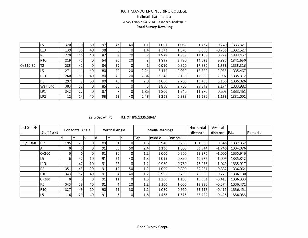
KATHMANDU ENGINEERING COLLEGEKalimati, Kathmandu
Survey Camp 2064, NEATC, Kharipati, Bhaktapur
Road Survey Detailing
L5 320 10 30 97 43 40 1.1 1.091 1.082 1.767 ‐0.240 1333.327L10 139 38 40 98 0 0 1.4 1.373 1.345 5.393 ‐0.758 1332.527R5 220 46 40 87 3 20 2 1.929 1.858 14.163 0.728 1333.457R10 219 47 0 54 50 20 3 2.895 2.790 14.036 9.887 1341.650
0+339.82 T2 285 41 0 84 59 0 1 0.910 0.820 17.862 1.568 1335.316L5 271 11 40 80 50 20 2.24 2.146 2.052 18.323 2.955 1335.467L10 260 55 40 80 48 20 2.34 2.248 2.156 17.930 2.902 1335.312R3 297 7 50 80 46 0 2.9 2.800 2.700 19.485 3.168 1335.026Wall End 303 52 0 85 50 0 3 2.850 2.700 29.842 2.174 1333.982LP1 342 27 0 87 7 0 1.86 1.800 1.740 11.970 0.603 1333.461LP2 12 14 40 95 25 40 2.46 2.398 2.336 12.289 ‐1.168 1331.092
Zero Set At:IP5 R.L.OF IP6:1336.586M
Inst.Stn./HI. Staff Point
Horizantal distance
Vertical distance R.L. Remarks
d m s d m s Top middle BottomIP6/1.360 IP7 195 23 0 89 51 0 1.6 0.940 0.280 131.999 0.346 1337.352
A 0 0 0 91 50 50 2.4 2.130 1.860 53.944 ‐1.740 1334.0760+360 0 0 0 91 26 0 1.2 1.000 0.800 39.975 ‐1.000 1335.946L5 6 42 10 91 24 40 1.3 1.095 0.890 40.975 ‐1.009 1335.842L10 11 47 10 91 22 0 1.2 0.980 0.760 43.975 ‐1.049 1335.917R5 351 45 20 91 15 50 1.2 1.000 0.800 39.981 ‐0.882 1336.064R10 343 52 40 91 4 40 1.2 0.995 0.790 40.985 ‐0.771 1336.1800+380 0 0 0 91 11 0 1.3 1.200 1.100 19.991 ‐0.413 1336.333R5 343 39 40 91 4 20 1.2 1.100 1.000 19.993 ‐0.374 1336.472R10 327 49 20 90 59 30 1.2 1.080 0.960 23.993 ‐0.415 1336.451L5 16 29 40 91 5 0 1.6 1.488 1.375 22.492 ‐0.425 1336.033
Horizontal Angle Vertical Angle Stadia Readings
Road Survey Gropu J
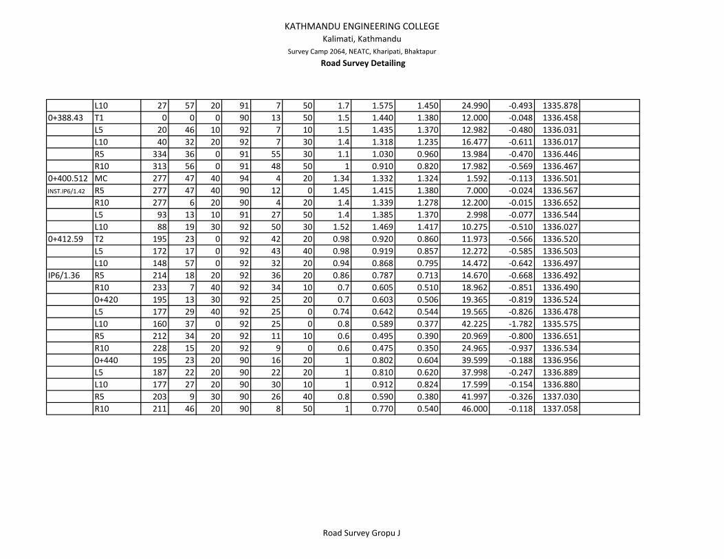
KATHMANDU ENGINEERING COLLEGEKalimati, Kathmandu
Survey Camp 2064, NEATC, Kharipati, Bhaktapur
Road Survey Detailing
L10 27 57 20 91 7 50 1.7 1.575 1.450 24.990 ‐0.493 1335.8780+388.43 T1 0 0 0 90 13 50 1.5 1.440 1.380 12.000 ‐0.048 1336.458
L5 20 46 10 92 7 10 1.5 1.435 1.370 12.982 ‐0.480 1336.031L10 40 32 20 92 7 30 1.4 1.318 1.235 16.477 ‐0.611 1336.017R5 334 36 0 91 55 30 1.1 1.030 0.960 13.984 ‐0.470 1336.446R10 313 56 0 91 48 50 1 0.910 0.820 17.982 ‐0.569 1336.467
0+400.512 MC 277 47 40 94 4 20 1.34 1.332 1.324 1.592 ‐0.113 1336.501INST.IP6/1.42 R5 277 47 40 90 12 0 1.45 1.415 1.380 7.000 ‐0.024 1336.567
R10 277 6 20 90 4 20 1.4 1.339 1.278 12.200 ‐0.015 1336.652L5 93 13 10 91 27 50 1.4 1.385 1.370 2.998 ‐0.077 1336.544L10 88 19 30 92 50 30 1.52 1.469 1.417 10.275 ‐0.510 1336.027
0+412.59 T2 195 23 0 92 42 20 0.98 0.920 0.860 11.973 ‐0.566 1336.520L5 172 17 0 92 43 40 0.98 0.919 0.857 12.272 ‐0.585 1336.503L10 148 57 0 92 32 20 0.94 0.868 0.795 14.472 ‐0.642 1336.497
IP6/1.36 R5 214 18 20 92 36 20 0.86 0.787 0.713 14.670 ‐0.668 1336.492R10 233 7 40 92 34 10 0.7 0.605 0.510 18.962 ‐0.851 1336.4900+420 195 13 30 92 25 20 0.7 0.603 0.506 19.365 ‐0.819 1336.524L5 177 29 40 92 25 0 0.74 0.642 0.544 19.565 ‐0.826 1336.478L10 160 37 0 92 25 0 0.8 0.589 0.377 42.225 ‐1.782 1335.575R5 212 34 20 92 11 10 0.6 0.495 0.390 20.969 ‐0.800 1336.651R10 228 15 20 92 9 0 0.6 0.475 0.350 24.965 ‐0.937 1336.5340+440 195 23 20 90 16 20 1 0.802 0.604 39.599 ‐0.188 1336.956L5 187 22 20 90 22 20 1 0.810 0.620 37.998 ‐0.247 1336.889L10 177 27 20 90 30 10 1 0.912 0.824 17.599 ‐0.154 1336.880R5 203 9 30 90 26 40 0.8 0.590 0.380 41.997 ‐0.326 1337.030R10 211 46 20 90 8 50 1 0.770 0.540 46.000 ‐0.118 1337.058
Road Survey Gropu J
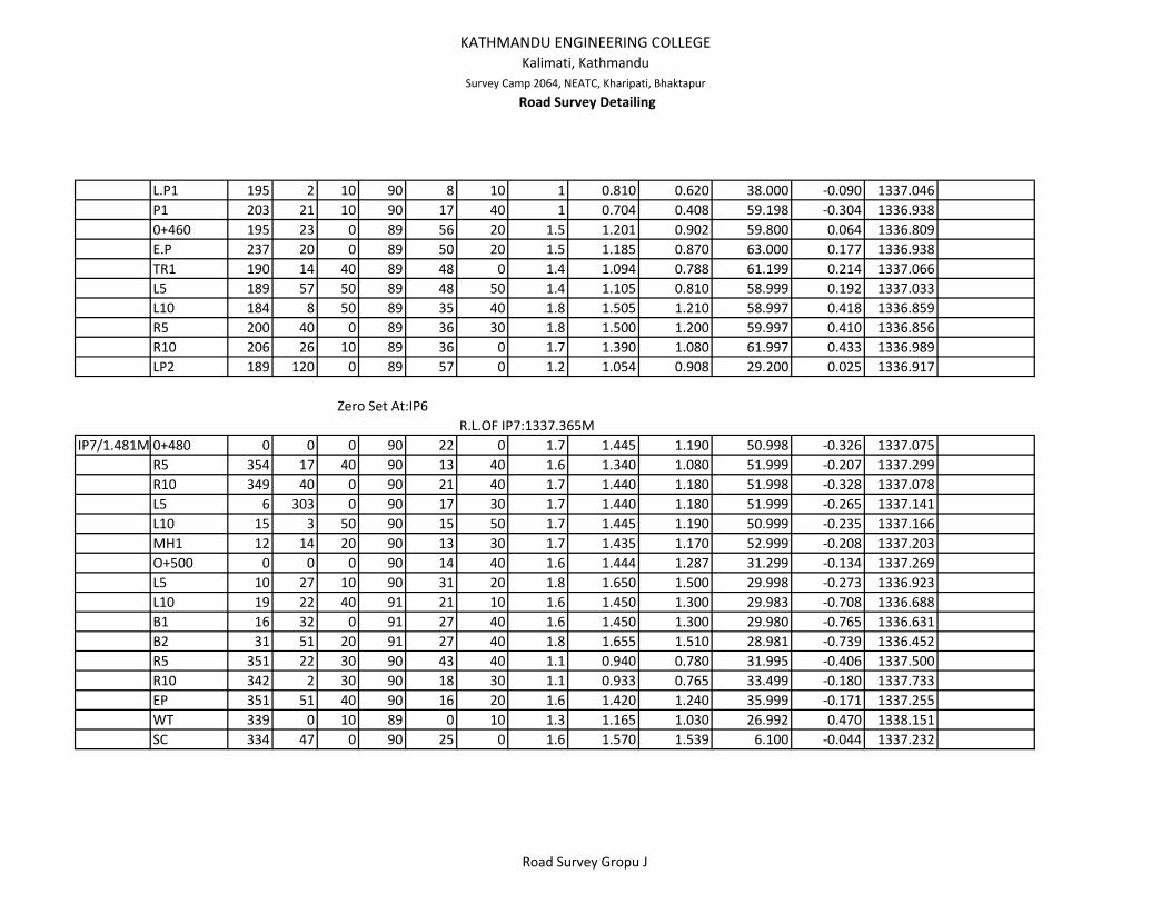
KATHMANDU ENGINEERING COLLEGEKalimati, Kathmandu
Survey Camp 2064, NEATC, Kharipati, Bhaktapur
Road Survey Detailing
L.P1 195 2 10 90 8 10 1 0.810 0.620 38.000 ‐0.090 1337.046P1 203 21 10 90 17 40 1 0.704 0.408 59.198 ‐0.304 1336.9380+460 195 23 0 89 56 20 1.5 1.201 0.902 59.800 0.064 1336.809E.P 237 20 0 89 50 20 1.5 1.185 0.870 63.000 0.177 1336.938TR1 190 14 40 89 48 0 1.4 1.094 0.788 61.199 0.214 1337.066L5 189 57 50 89 48 50 1.4 1.105 0.810 58.999 0.192 1337.033L10 184 8 50 89 35 40 1.8 1.505 1.210 58.997 0.418 1336.859R5 200 40 0 89 36 30 1.8 1.500 1.200 59.997 0.410 1336.856R10 206 26 10 89 36 0 1.7 1.390 1.080 61.997 0.433 1336.989LP2 189 120 0 89 57 0 1.2 1.054 0.908 29.200 0.025 1336.917
Zero Set At:IP6R.L.OF IP7:1337.365M
IP7/1.481M 0+480 0 0 0 90 22 0 1.7 1.445 1.190 50.998 ‐0.326 1337.075R5 354 17 40 90 13 40 1.6 1.340 1.080 51.999 ‐0.207 1337.299R10 349 40 0 90 21 40 1.7 1.440 1.180 51.998 ‐0.328 1337.078L5 6 303 0 90 17 30 1.7 1.440 1.180 51.999 ‐0.265 1337.141L10 15 3 50 90 15 50 1.7 1.445 1.190 50.999 ‐0.235 1337.166MH1 12 14 20 90 13 30 1.7 1.435 1.170 52.999 ‐0.208 1337.203O+500 0 0 0 90 14 40 1.6 1.444 1.287 31.299 ‐0.134 1337.269L5 10 27 10 90 31 20 1.8 1.650 1.500 29.998 ‐0.273 1336.923L10 19 22 40 91 21 10 1.6 1.450 1.300 29.983 ‐0.708 1336.688B1 16 32 0 91 27 40 1.6 1.450 1.300 29.980 ‐0.765 1336.631B2 31 51 20 91 27 40 1.8 1.655 1.510 28.981 ‐0.739 1336.452R5 351 22 30 90 43 40 1.1 0.940 0.780 31.995 ‐0.406 1337.500R10 342 2 30 90 18 30 1.1 0.933 0.765 33.499 ‐0.180 1337.733EP 351 51 40 90 16 20 1.6 1.420 1.240 35.999 ‐0.171 1337.255WT 339 0 10 89 0 10 1.3 1.165 1.030 26.992 0.470 1338.151SC 334 47 0 90 25 0 1.6 1.570 1.539 6.100 ‐0.044 1337.232
Road Survey Gropu J

KATHMANDU ENGINEERING COLLEGEKalimati, Kathmandu
Survey Camp 2064, NEATC, Kharipati, Bhaktapur
Road Survey Detailing
EP3 310 58 0 90 10 10 1.4 1.368 1.336 6.400 ‐0.019 1337.459EP4 309 18 0 90 11 10 1.4 1.378 1.355 4.500 ‐0.015 1337.4540+525T1 359 28 20 90 22 0 1.6 1.570 1.539 6.100 ‐0.039 1337.237R5 309 18 0 90 11 10 1.4 1.378 1.355 4.500 ‐0.015 1337.454R10 283 6 20 90 27 20 1.5 1.459 1.418 8.199 ‐0.065 1337.322L5 21 40 20 90 0 40 1.6 1.559 1.517 8.300 ‐0.002 1337.286L10 32 40 40 93 38 40 1.6 1.537 1.474 12.549 ‐0.799 1336.510MC 71 10 40 89 39 0 1.5 1.494 1.488 1.200 0.007 1337.359L5 61 30 0 89 58 0 1.6 1.570 1.540 6.000 0.003 1337.279L10 58 5 0 89 40 0 1.8 1.742 1.684 11.600 0.067 1337.171R5 245 20 0 89 13 20 1.5 1.477 1.454 4.599 0.062 1337.431R10 249 30 0 88 47 0 1.4 1.357 1.313 8.696 0.185 1337.674CN520 0 0 0 88 57 30 1.94 1.885 1.830 10.996 0.200 1337.161R5 336 13 30 88 57 30 1.89 1.826 1.762 12.796 0.233 1337.253R10 316 16 30 88 51 40 1.8 1.730 1.660 13.994 0.278 1337.394L5 21 15 50 89 23 10 1.9 1.835 1.770 12.999 0.139 1337.150L10 31 46 40 93 35 30 1.45 1.370 1.290 15.937 ‐1.000 1336.476BC1 32 40 40 93 38 40 1.6 1.537 1.474 12.549 ‐0.799 1336.510MH2 355 51 40 30 39 0 1.4 1.278 1.155 6.367 10.745 1348.314MH1 358 37 10 90 25 20 1.4 1.265 1.130 26.999 ‐0.199 1337.382
536.715M T2 136 46 0 88 55 40 1.6 1.570 1.540 5.998 0.112 1337.388L5 100 17 40 88 49 20 1.8 1.757 1.713 8.696 0.179 1337.268L10 78 40 0 88 45 10 1.9 1.830 1.760 13.993 0.305 1337.321R5 176 6 0 88 33 30 1.4 1.365 1.330 6.996 0.176 1337.657WALL1 180 9 0 88 28 20 1.7 1.615 1.530 16.988 0.453 1337.684POLE1 157 51 40 88 75 50 1.7 1.615 1.530 16.997 0.218 1337.449
Road Survey Gropu J

KATHMANDU ENGINEERING COLLEGEKalimati, Kathmandu
Survey Camp 2064, NEATC, Kharipati, Bhaktapur
Road Survey Detailing
540 136 33 30 88 40 100 1.7 1.651 1.602 9.795 0.223 1337.418L5 104 18 20 88 53 20 1.8 1.733 1.665 13.495 0.262 1337.375L10 87 12 50 88 44 0 1.9 1.821 1.742 15.792 0.349 1337.374
BOUNDING R5 120 28 0 88 26 40 1.8 1.738 1.676 12.391 0.336 1337.444MH3 94 31 0 98 42 0 1.9 1.813 1.725 17.100 ‐2.617 1334.417BC2 76 40 40 93 1 0 1.5 1.412 1.323 17.651 ‐0.930 1336.504EP 134 2 40 89 27 30 1.6 1.435 1.270 32.997 0.312 1337.723IP8 136 14 10 89 42 20 1.7 1.365 1.030 66.998 0.344 1337.825
560 136 36 20 89 15 10 1.9 1.785 1.670 22.996 0.300 1337.361560 R5 148 30 40 88 57 0 1.8 1.653 1.505 29.490 0.540 1337.734
R10 152 8 20 88 49 0 1.7 1.555 1.410 28.988 0.599 1337.890 wall endL5 125 4 0 89 25 20 1.9 1.750 1.600 29.997 0.303 1337.399L10 113 35 0 89 49 10 1.9 1.750 1.600 30.000 0.095 1337.191
Zero Set At:IP7 R.L.OF IP8:1337.807MInst.Stn./HI. Staff Point
Horizantal distance
Vertical distance R.L. Remarks
d m s d m s Top middle BottomIP8/1.40 IP9 151 0 30 89 20 0 1.5 1.143 0.786 71.390 0.831 1338.895m 0+580 0 0 0 89 54 0 1.8 1.713 1.626 17.400 0.030 1337.524
L5 19 42 40 89 58 0 1.8 1.706 1.612 18.800 0.011 1337.512L10 32 27 0 90 2 20 1.8 1.694 1.587 21.300 ‐0.014 1337.499R5 343 12 0 89 53 0 1.7 1.610 1.520 18.000 0.037 1337.634R10 323 45 40 89 52 40 1.7 1.603 1.506 19.400 0.041 1337.645
0+591.734 T1 0 0 0 95 42 40 1.21 1.185 1.159 5.049 ‐0.505 1337.518L5 48 26 20 92 50 20 1.22 1.178 1.135 8.479 ‐0.420 1337.609L10 59 47 0 92 41 0 1.1 1.023 0.946 15.366 ‐0.720 1337.464
Horizontal Angle Vertical Angle Stadia Readings
Road Survey Gropu J
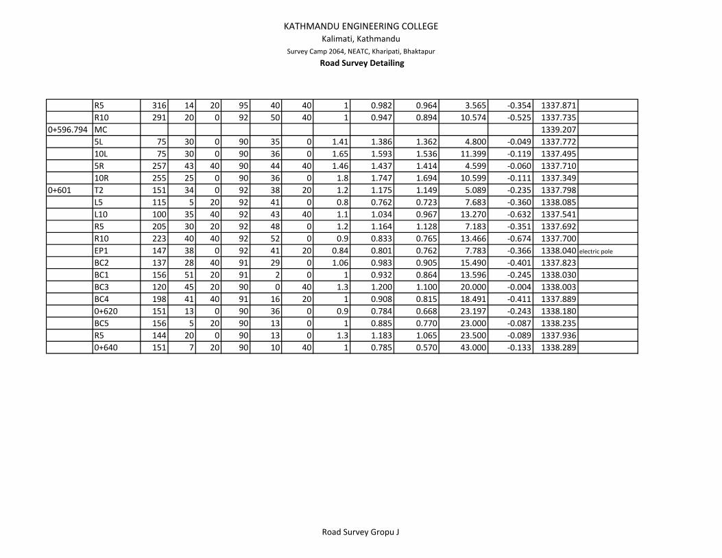
KATHMANDU ENGINEERING COLLEGEKalimati, Kathmandu
Survey Camp 2064, NEATC, Kharipati, Bhaktapur
Road Survey Detailing
R5 316 14 20 95 40 40 1 0.982 0.964 3.565 ‐0.354 1337.871R10 291 20 0 92 50 40 1 0.947 0.894 10.574 ‐0.525 1337.735
0+596.794 MC 1339.2075L 75 30 0 90 35 0 1.41 1.386 1.362 4.800 ‐0.049 1337.77210L 75 30 0 90 36 0 1.65 1.593 1.536 11.399 ‐0.119 1337.4955R 257 43 40 90 44 40 1.46 1.437 1.414 4.599 ‐0.060 1337.71010R 255 25 0 90 36 0 1.8 1.747 1.694 10.599 ‐0.111 1337.349
0+601 T2 151 34 0 92 38 20 1.2 1.175 1.149 5.089 ‐0.235 1337.798L5 115 5 20 92 41 0 0.8 0.762 0.723 7.683 ‐0.360 1338.085L10 100 35 40 92 43 40 1.1 1.034 0.967 13.270 ‐0.632 1337.541R5 205 30 20 92 48 0 1.2 1.164 1.128 7.183 ‐0.351 1337.692R10 223 40 40 92 52 0 0.9 0.833 0.765 13.466 ‐0.674 1337.700EP1 147 38 0 92 41 20 0.84 0.801 0.762 7.783 ‐0.366 1338.040 electric pole
BC2 137 28 40 91 29 0 1.06 0.983 0.905 15.490 ‐0.401 1337.823BC1 156 51 20 91 2 0 1 0.932 0.864 13.596 ‐0.245 1338.030BC3 120 45 20 90 0 40 1.3 1.200 1.100 20.000 ‐0.004 1338.003BC4 198 41 40 91 16 20 1 0.908 0.815 18.491 ‐0.411 1337.8890+620 151 13 0 90 36 0 0.9 0.784 0.668 23.197 ‐0.243 1338.180BC5 156 5 20 90 13 0 1 0.885 0.770 23.000 ‐0.087 1338.235R5 144 20 0 90 13 0 1.3 1.183 1.065 23.500 ‐0.089 1337.9360+640 151 7 20 90 10 40 1 0.785 0.570 43.000 ‐0.133 1338.289
Road Survey Gropu J

KATHMANDU ENGINEERING COLLEGEKalimati, Kathmandu
Survey Camp 2064, NEATC, Kharipati, Bhaktapur
Road Survey Detailing
Zero Set At:IP8 R.L.OF IP9:1338.922MInst.Stn./HI. Staff Point
Horizantal distance
Vertical distance R.L. Remarks
d m s d m s Top middle BottomIP9/1.48 IP10 106 44 20 91 9 50 1.5 1.218 0.936 56.377 ‐1.145 1338.039
0+640 0 0 0 90 49 10 1.8 1.655 1.510 28.994 ‐0.415 1338.332L5 11 15 0 90 54 20 1.7 1.560 1.420 27.993 ‐0.442 1338.400L10 21 30 0 90 55 50 1.7 1.548 1.396 30.392 ‐0.494 1338.360R5 349 7 10 91 1 50 1.8 1.658 1.515 28.491 ‐0.513 1338.232R10 335 14 30 91 14 30 1.9 1.750 1.600 29.986 ‐0.650 1338.002T1 0 0 0 91 23 30 1.6 1.490 1.380 21.987 ‐0.534 1338.378R5 348 3 40 91 27 30 1.7 1.591 1.482 21.786 ‐0.555 1338.256R10 332 39 10 91 32 0 1.7 1.570 1.440 25.981 ‐0.695 1338.137L5 14 56 40 91 31 20 1.4 1.290 1.180 21.984 ‐0.584 1338.528 R1L10 30 38 40 91 26 40 1.3 1.180 1.060 23.985 ‐0.605 1338.617 R2(TREE)B1 3 10 20 91 29 30 1.5 1.305 1.110 38.974 ‐1.015 1338.082 B1B2 355 25 10 90 21 10 2.1 1.905 1.710 38.999 ‐0.240 1338.257 B2B3 20 39 50 91 42 30 1.3 1.100 0.900 39.964 ‐1.192 1338.110 B3B4 339 14 40 91 40 10 1.5 1.285 1.070 42.964 ‐1.252 1337.865 B4P1 352 53 40 91 47 0 1.2 1.073 0.945 25.475 ‐0.793 1338.536 pole10+660 19 29 30 91 53 30 1.8 1.753 1.705 9.490 ‐0.313 1338.336R5 340 56 0 91 25 40 1.6 1.574 1.548 5.197 ‐0.130 1338.698R10 285 15 50 91 20 10 1.4 1.369 1.338 6.197 ‐0.145 1338.888P1 318 3 0 91 35 40 1.5 1.459 1.418 8.194 ‐0.228 1338.715L5 26 6 30 95 30 20 0.9 0.820 0.740 15.853 ‐1.528 1338.054L10 34 15 0 92 5 20 1 0.887 0.774 22.570 ‐0.823 1338.692
0+665 MC 53 23 20 92 5 20 1.9 1.864 1.828 7.190 ‐0.262 1338.276R5 56 7 40 92 50 20 1.7 1.690 1.680 1.995 ‐0.099 1338.613R10 247 13 0 91 49 10 1.7 1.687 1.673 2.697 ‐0.086 1338.630
Horizontal Angle Vertical Angle Stadia Readings
Road Survey Gropu J

KATHMANDU ENGINEERING COLLEGEKalimati, Kathmandu
Survey Camp 2064, NEATC, Kharipati, Bhaktapur
Road Survey Detailing
L5 53 4 10 92 11 0 1.9 1.837 1.774 12.582 ‐0.480 1338.085L10 54 19 50 92 24 40 1 0.913 0.826 17.369 ‐0.731 1338.758 R40+680 105 17 50 92 27 10 1.4 1.315 1.230 16.969 ‐0.727 1338.360R5 123 3 20 90 26 10 0.8 0.705 0.609 19.099 ‐0.145 1339.552R10 138 31 10 87 39 10 1.3 1.192 1.083 21.664 0.888 1340.098 WallL5 89 22 10 89 69 10 1.5 1.408 1.315 18.500 ‐0.049 1338.945 road outL10 74 35 0 90 11 10 1.7 1.593 1.485 21.500 ‐0.070 1338.740 road out
0+684.48 T2 107 5 10 90 19 40 1 0.890 0.780 21.999 ‐0.126 1339.386R5 122 43 30 88 2 40 1.4 1.280 1.160 23.972 0.819 1339.941 road inG1 127 2 10 87 30 10 1.3 1.180 1.060 23.954 1.045 1340.267 GateL5 87 56 50 90 40 10 1.3 1.187 1.074 22.597 ‐0.264 1338.951 road inL10 69 45 0 90 45 0 1.8 1.683 1.565 23.496 ‐0.308 1338.412
Zero Set At:IP9 R.L.OF IP10:1338.922MInst.Stn./HI. Staff Point
Horizantal distance
Vertical distance R.L. Remarks
d m s d m s Top middle BottomIP10/1.35 IP9 159 38 40 88 43 40 1 0.690 0.380 61.969 1.376 1340.958
0+700 0 0 0 90 56 20 1 0.905 0.810 18.995 ‐0.311 1339.056R5 343 23 10 90 46 10 1 0.898 0.796 20.396 ‐0.274 1339.100R10 333 15 30 87 24 20 1.2 1.083 0.966 23.352 1.058 1340.247 WALL(W1)L5 16 8 10 92 1 10 0.7 0.603 0.505 19.476 ‐0.687 1338.983L10 29 34 50 91 43 30 1 0.895 0.790 20.981 ‐0.632 1338.745B 39 31 50 91 49 40 2.2 2.110 2.020 17.982 ‐0.574 1337.588 BT1 0 0 0 91 51 20 1 0.955 0.910 8.991 ‐0.291 1339.026R5 328 57 20 91 32 30 1 0.950 0.899 10.093 ‐0.272 1339.051R10 312 17 20 88 3 20 1.6 1.540 1.480 11.986 0.407 1339.139 W2L5 32 41 40 87 53 40 1.9 1.848 1.795 10.486 0.386 1338.810L10 50 13 0 90 55 50 2.6 2.525 2.450 14.996 ‐0.244 1337.503 B2
Horizontal Angle Vertical Angle Stadia Readings
Road Survey Gropu J
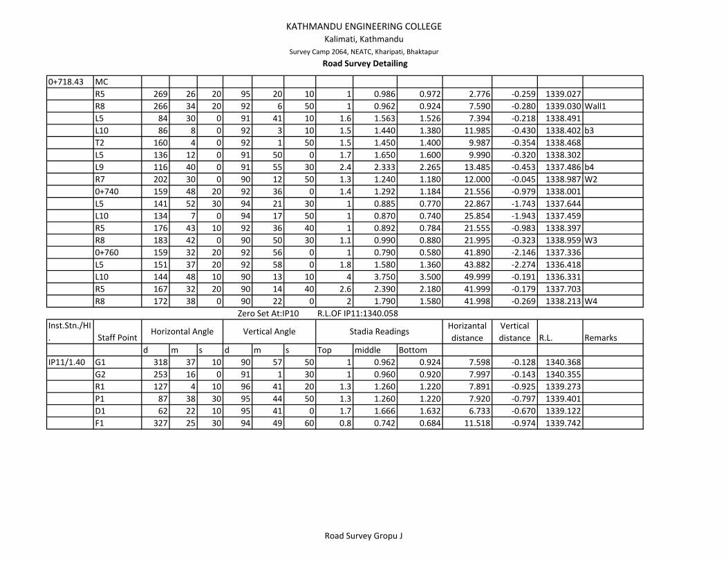
KATHMANDU ENGINEERING COLLEGEKalimati, Kathmandu
Survey Camp 2064, NEATC, Kharipati, Bhaktapur
Road Survey Detailing
0+718.43 MCR5 269 26 20 95 20 10 1 0.986 0.972 2.776 ‐0.259 1339.027R8 266 34 20 92 6 50 1 0.962 0.924 7.590 ‐0.280 1339.030 Wall1L5 84 30 0 91 41 10 1.6 1.563 1.526 7.394 ‐0.218 1338.491L10 86 8 0 92 3 10 1.5 1.440 1.380 11.985 ‐0.430 1338.402 b3T2 160 4 0 92 1 50 1.5 1.450 1.400 9.987 ‐0.354 1338.468L5 136 12 0 91 50 0 1.7 1.650 1.600 9.990 ‐0.320 1338.302L9 116 40 0 91 55 30 2.4 2.333 2.265 13.485 ‐0.453 1337.486 b4R7 202 30 0 90 12 50 1.3 1.240 1.180 12.000 ‐0.045 1338.987 W20+740 159 48 20 92 36 0 1.4 1.292 1.184 21.556 ‐0.979 1338.001L5 141 52 30 94 21 30 1 0.885 0.770 22.867 ‐1.743 1337.644L10 134 7 0 94 17 50 1 0.870 0.740 25.854 ‐1.943 1337.459R5 176 43 10 92 36 40 1 0.892 0.784 21.555 ‐0.983 1338.397R8 183 42 0 90 50 30 1.1 0.990 0.880 21.995 ‐0.323 1338.959 W30+760 159 32 20 92 56 0 1 0.790 0.580 41.890 ‐2.146 1337.336L5 151 37 20 92 58 0 1.8 1.580 1.360 43.882 ‐2.274 1336.418L10 144 48 10 90 13 10 4 3.750 3.500 49.999 ‐0.191 1336.331R5 167 32 20 90 14 40 2.6 2.390 2.180 41.999 ‐0.179 1337.703R8 172 38 0 90 22 0 2 1.790 1.580 41.998 ‐0.269 1338.213 W4
Zero Set At:IP10 R.L.OF IP11:1340.058Inst.Stn./HI. Staff Point
Horizantal distance
Vertical distance R.L. Remarks
d m s d m s Top middle BottomIP11/1.40 G1 318 37 10 90 57 50 1 0.962 0.924 7.598 ‐0.128 1340.368
G2 253 16 0 91 1 30 1 0.960 0.920 7.997 ‐0.143 1340.355R1 127 4 10 96 41 20 1.3 1.260 1.220 7.891 ‐0.925 1339.273P1 87 38 30 95 44 50 1.3 1.260 1.220 7.920 ‐0.797 1339.401D1 62 22 10 95 41 0 1.7 1.666 1.632 6.733 ‐0.670 1339.122F1 327 25 30 94 49 60 0.8 0.742 0.684 11.518 ‐0.974 1339.742
Horizontal Angle Vertical Angle Stadia Readings
Road Survey Gropu J

KATHMANDU ENGINEERING COLLEGEKalimati, Kathmandu
Survey Camp 2064, NEATC, Kharipati, Bhaktapur
Road Survey Detailing
L1 328 33 40 95 2 50 2.5 2.415 2.330 16.868 ‐1.490 1337.553L2 62 35 0 98 12 40 3.92 3.840 3.760 15.674 ‐2.262 1335.356
Road Survey Gropu J
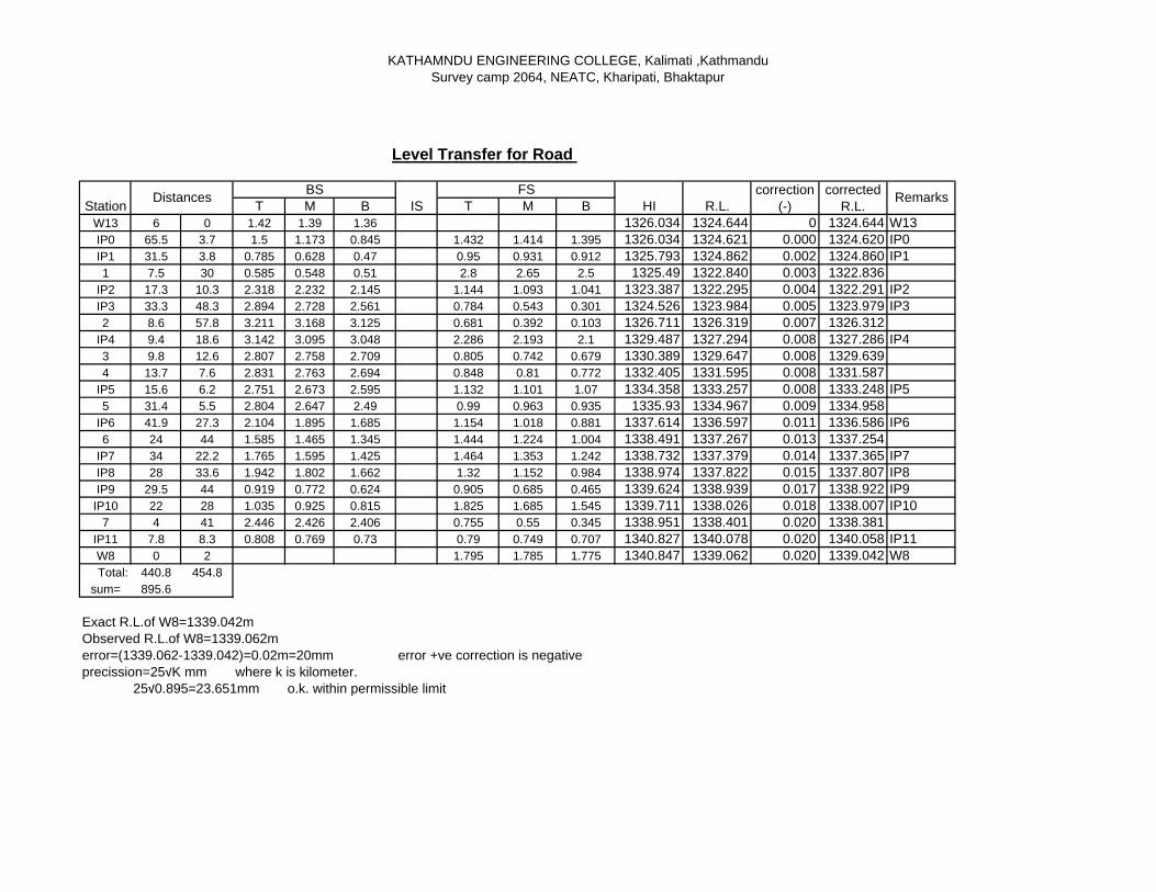
KATHAMNDU ENGINEERING COLLEGE, Kalimati ,KathmanduSurvey camp 2064, NEATC, Kharipati, Bhaktapur
T M B T M BW13 6 0 1.42 1.39 1.36 1326.034 1324.644 0 1324.644 W13IP0 65.5 3.7 1.5 1.173 0.845 1.432 1.414 1.395 1326.034 1324.621 0.000 1324.620 IP0IP1 31.5 3.8 0.785 0.628 0.47 0.95 0.931 0.912 1325.793 1324.862 0.002 1324.860 IP11 7.5 30 0.585 0.548 0.51 2.8 2.65 2.5 1325.49 1322.840 0.003 1322.836
IP2 17.3 10.3 2.318 2.232 2.145 1.144 1.093 1.041 1323.387 1322.295 0.004 1322.291 IP2IP3 33.3 48.3 2.894 2.728 2.561 0.784 0.543 0.301 1324.526 1323.984 0.005 1323.979 IP32 8.6 57.8 3.211 3.168 3.125 0.681 0.392 0.103 1326.711 1326.319 0.007 1326.312
IP4 9.4 18.6 3.142 3.095 3.048 2.286 2.193 2.1 1329.487 1327.294 0.008 1327.286 IP43 9.8 12.6 2.807 2.758 2.709 0.805 0.742 0.679 1330.389 1329.647 0.008 1329.6394 13.7 7.6 2.831 2.763 2.694 0.848 0.81 0.772 1332.405 1331.595 0.008 1331.587
IP5 15.6 6.2 2.751 2.673 2.595 1.132 1.101 1.07 1334.358 1333.257 0.008 1333.248 IP55 31.4 5.5 2.804 2.647 2.49 0.99 0.963 0.935 1335.93 1334.967 0.009 1334.958
IP6 41.9 27.3 2.104 1.895 1.685 1.154 1.018 0.881 1337.614 1336.597 0.011 1336.586 IP66 24 44 1.585 1.465 1.345 1.444 1.224 1.004 1338.491 1337.267 0.013 1337.254
IP7 34 22.2 1.765 1.595 1.425 1.464 1.353 1.242 1338.732 1337.379 0.014 1337.365 IP7IP8 28 33.6 1.942 1.802 1.662 1.32 1.152 0.984 1338.974 1337.822 0.015 1337.807 IP8IP9 29.5 44 0.919 0.772 0.624 0.905 0.685 0.465 1339.624 1338.939 0.017 1338.922 IP9
IP10 22 28 1.035 0.925 0.815 1.825 1.685 1.545 1339.711 1338.026 0.018 1338.007 IP107 4 41 2.446 2.426 2.406 0.755 0.55 0.345 1338.951 1338.401 0.020 1338.381
IP11 7.8 8.3 0.808 0.769 0.73 0.79 0.749 0.707 1340.827 1340.078 0.020 1340.058 IP11W8 0 2 1.795 1.785 1.775 1340.847 1339.062 0.020 1339.042 W8Total: 440.8 454.8
sum= 895.6
Exact R.L.of W8=1339.042mObserved R.L.of W8=1339.062merror=(1339.062-1339.042)=0.02m=20mm error +ve correction is negativeprecission=25√K mm where k is kilometer.
25√0.895=23.651mm o.k. within permissible limit
RemarksBS FSDistances corrected R.L.
correction(-)Station IS HI R.L.
Level Transfer for Road

s.n.Total length
Mean Length Precision
From To1 Q6 Q4 77.36 77.35 1 in 38672 Q4 Q6 77.343 Q1 Q2 91.1 91.09 1 IN 45544 Q2 Q1 91.085 Q4 TBM 23.43 23.425 1 IN 23426 TBM Q4 23.42
Bearing of Q4-TBM =236˚ (wcb)
S.N. Leg L1 L2 Mean Remarks1 46 77.35 77.35 Q4Q62 12 91.09 91.09 Q1Q23 16 73.094 73.094 Q1Q64 14 54.933 54.948 54.875 54.902 54.915 Q1Q45 36 32.849 32.819 32.834 Q3Q66 13 68.885 68.887 68.886 Q1Q37 24 118.162 118.162 Q2Q48 25 128.754 128.68 128.717 Q2Q59 45 107.846 107.84 107.843 Q4Q510 34 94.789 94.789 Q3Q411 15 141.674 141.674 Q1Q5
Station distances (m)
DISTANCE MEASUREMENT SHEET FOR BRIDGE:
Length calculation by using Sine Law to the triangles
27.74+26.13+13.92+9.5725.64+24.35+8.65+18.7
27.64+25.68+20.34+17.4426.35+28.49+22.36+13.88
9.3+7.82+6.3110.3+7.5+5.62
Remarks
o.k. within precision
o.k. within precision
o.k. within precision
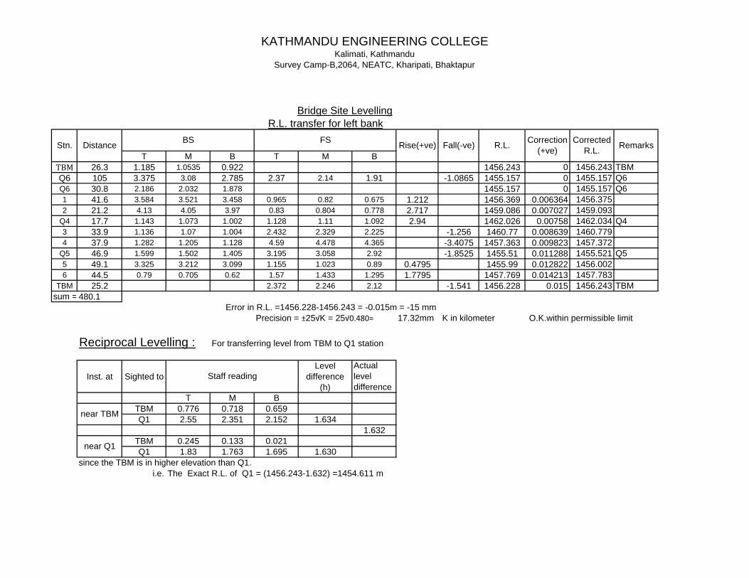
KATHMANDU ENGINEERING COLLEGE Kalimati, Kathmandu
Survey Camp-B,2064, NEATC, Kharipati, Bhaktapur
R.L. transfer for left bank
T M B T M BTBM 26.3 1.185 1.0535 0.922 1456.243 0 1456.243 TBMQ6 105 3.375 3.08 2.785 2.37 2.14 1.91 -1.0865 1455.157 0 1455.157 Q6Q6 30.8 2.186 2.032 1.878 1455.157 0 1455.157 Q61 41.6 3.584 3.521 3.458 0.965 0.82 0.675 1.212 1456.369 0.006364 1456.3752 21.2 4.13 4.05 3.97 0.83 0.804 0.778 2.717 1459.086 0.007027 1459.093
Q4 17.7 1.143 1.073 1.002 1.128 1.11 1.092 2.94 1462.026 0.00758 1462.034 Q43 33.9 1.136 1.07 1.004 2.432 2.329 2.225 -1.256 1460.77 0.008639 1460.7794 37.9 1.282 1.205 1.128 4.59 4.478 4.365 -3.4075 1457.363 0.009823 1457.372
Q5 46.9 1.599 1.502 1.405 3.195 3.058 2.92 -1.8525 1455.51 0.011288 1455.521 Q55 49.1 3.325 3.212 3.099 1.155 1.023 0.89 0.4795 1455.99 0.012822 1456.0026 44.5 0.79 0.705 0.62 1.57 1.433 1.295 1.7795 1457.769 0.014213 1457.783
TBM 25.2 2.372 2.246 2.12 -1.541 1456.228 0.015 1456.243 TBMsum = 480.1
Precision = ±25√K = 25√0.480= 17.32mm K in kilometer O.K.within permissible limit
Reciprocal Levelling : For transferring level from TBM to Q1 station
Inst. at Sighted toLevel
difference (h)
Actual level difference
T M BTBM 0.776 0.718 0.659Q1 2.55 2.351 2.152 1.634
1.632TBM 0.245 0.133 0.021Q1 1.83 1.763 1.695 1.630
since the TBM is in higher elevation than Q1.i.e. The Exact R.L. of Q1 = (1456.243-1.632) =1454.611 m
Error in R.L. =1456.228-1456.243 = -0.015m = -15 mm
Staff reading
near TBM
near Q1
Stn. Distance BS FS Rise(+ve) RemarksFall(-ve) R.L. Correction(+ve)
Bridge Site Levelling
Corrected R.L.

KATHMANDU ENGINEERING COLLEGE Kalimati, Kathmandu
Survey Camp-B,2064, NEATC, Kharipati, Bhaktapur
Bridge Site Levelling
T M B T M BQ1 34.2 1.608 1.437 1.266 1454.611 0 1454.611 Q1Q3 69.6 1.596 1.425 1.254 1.619 1.442 1.265 -0.005 1454.606 0.000976 1454.607 Q37 72.2 1.75 1.55 1.35 1.664 1.503 1.342 -0.078 1454.528 0.001656 1454.53
Q2 102.9 1.705 1.453 1.201 1.765 1.503 1.24 0.0475 1454.576 0.002624 1454.578 Q2Q1 40 1.621 1.421 1.221 0.032 1454.608 0.003 1454.611 Q1
Sum= 318.9Error in R.L. =1454.608-1454.611 = -0.003m= -3 mm
Precision = ±25√K = 25√0.318= 14.0978mm K in kilometer O.K.within permissible limit
Distance BS Remarks
For Right Bank R.L. Transfer
R.L.FS Rise Fall Correction(+ve)
Corrected R.L.
Stn.
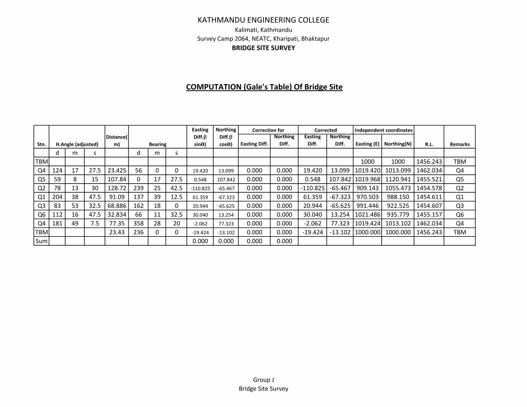
KATHMANDU ENGINEERING COLLEGEKalimati, Kathmandu
Survey Camp 2064, NEATC, Kharipati, BhaktapurBRIDGE SITE SURVEY
Easting Diff.Northing Diff.
Easting Diff.
Northing Diff. Easting (E) Northing(N)
d m s d m sTBM 1000 1000 1456.243 TBMQ4 124 17 27.5 23.425 56 0 0 19.420 13.099 0.000 0.000 19.420 13.099 1019.420 1013.099 1462.034 Q4Q5 59 8 15 107.84 0 17 27.5 0.548 107.842 0.000 0.000 0.548 107.842 1019.968 1120.941 1455.521 Q5Q2 78 13 30 128.72 239 25 42.5 ‐110.825 ‐65.467 0.000 0.000 ‐110.825 ‐65.467 909.143 1055.473 1454.578 Q2Q1 204 38 47.5 91.09 137 39 12.5 61.359 ‐67.323 0.000 0.000 61.359 ‐67.323 970.503 988.150 1454.611 Q1Q3 83 53 32.5 68.886 162 18 0 20.944 ‐65.625 0.000 0.000 20.944 ‐65.625 991.446 922.525 1454.607 Q3Q6 112 16 47.5 32.834 66 11 32.5 30.040 13.254 0.000 0.000 30.040 13.254 1021.486 935.779 1455.157 Q6Q4 181 49 7.5 77.35 358 28 20 ‐2.062 77.323 0.000 0.000 ‐2.062 77.323 1019.424 1013.102 1462.034 Q4TBM 23.43 236 0 0 ‐19.424 ‐13.102 0.000 0.000 ‐19.424 ‐13.102 1000.000 1000.000 1456.243 TBMSum 0.000 0.000 0.000 0.000
Remarks
Northing Diff.(l cosѲ)
COMPUTATION (Gale's Table) Of Bridge Site
Stn. H.Angle (adjusted)Distance(
m) Bearing
Easting Diff.(l sinѲ)
Correction for Corrected Independent coordinates
R.L.
Group JBridge Site Survey
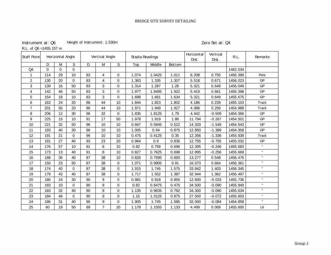
BRIDGE SITE SURVEY DETAILING
Instrument at: Q6 Zero Set at: Q4R.L. of Q6 =1455.157 m
Staff Point Stadia Readings Horizontal
Dist.Vertical
Dist.R.L. Remarks
D M S D M S Top Middle BottomQ4 0 0 0 1462.0341 114 29 10 83 4 0 1.074 1.0425 1.011 6.208 0.755 1456.399 Pole
2 130 20 0 83 4 0 1.363 1.335 1.307 5.518 0.671 1456.023 GP
3 139 16 50 83 3 0 1.314 1.287 1.26 5.321 0.649 1456.049 GP
4 142 46 50 83 3 0 1.977 1.9495 1.922 5.419 0.661 1455.398 GP
5 154 18 10 83 3 0 1.688 1.661 1.634 5.321 0.649 1455.675 GP
6 163 24 20 86 44 10 1.844 1.823 1.802 4.186 0.239 1455.103 Track
7 201 55 20 86 44 10 1.971 1.949 1.927 4.386 0.250 1454.988 Track
8 206 12 30 96 32 0 1.835 1.8125 1.79 4.442 -0.509 1454.366 GP
9 225 15 10 91 17 50 1.978 1.919 1.86 11.794 -0.267 1454.501 GP
10 221 32 50 96 10 10 0.667 0.5945 0.522 14.333 -1.549 1454.543 GP
11 193 40 30 96 10 10 1.005 0.94 0.875 12.850 -1.389 1454.358 GP
12 191 21 0 96 10 10 0.475 0.4125 0.35 12.356 -1.336 1454.939 Track
13 181 27 40 93 23 20 0.964 0.9 0.836 12.755 -0.755 1455.032 GP
14 176 57 10 91 8 10 0.82 0.758 0.696 12.395 -0.246 1455.683 "
15 173 13 40 91 8 10 0.827 0.7625 0.698 12.895 -0.256 1455.669 "
16 168 36 40 87 38 10 0.826 0.7595 0.693 13.277 0.548 1456.476 "
17 150 23 50 87 38 0 1.071 0.9905 0.91 16.073 0.664 1456.361 "
18 174 40 0 87 38 0 1.915 1.745 1.575 33.942 1.403 1456.345 "
19 179 43 40 87 38 0 1.717 1.552 1.387 32.944 1.362 1456.497 "
20 180 24 30 90 9 0 0.981 0.918 0.855 12.600 -0.033 1455.736 "
21 183 10 0 90 9 0 0.82 0.6475 0.475 34.500 -0.090 1455.949 "
22 183 32 40 90 9 0 1.135 0.9635 0.792 34.300 -0.090 1455.634 "
23 184 46 0 90 9 0 1.15 1.0125 0.875 27.500 -0.072 1455.603 "
24 186 31 40 90 9 0 1.905 1.745 1.585 32.000 -0.084 1454.858 "
25 60 19 50 89 7 20 1.178 1.1555 1.133 4.499 0.069 1455.600 L6
Height of Instrument: 1.530m
Horizontal Angle Vertical Angle
Group J

BRIDGE SITE SURVEY DETAILING
26 61 47 40 89 7 20 0.747 0.7225 0.698 4.899 0.075 1456.040 L7
27 68 16 10 89 7 20 0.959 0.93 0.901 5.799 0.089 1455.846 L8
28 70 2 10 89 7 20 0.325 0.295 0.265 5.999 0.092 1456.484 L9
29 82 46 10 89 7 20 0.507 0.4515 0.396 11.097 0.170 1456.406 L10
Instrument at: Q4 Zero Set at: Q6R.L. of Q4 =1462.034 m
Staff Point Stadia Readings Horizontal
Dist.Vertical
Dist.R.L. Remarks
D M S D M S Top Middle Bottom1 70 23 10 102 54 30 3.2 3.0725 2.945 24.227 -5.553 1454.8192 71 56 30 102 56 30 3.4 3.3 3.2 18.997 -4.365 1455.7793 67 36 30 102 58 10 2.4 2.33 2.26 13.295 -3.062 1458.0524 66 59 0 103 12 0 2.6 2.56 2.52 7.583 -1.779 1459.1055 70 13 40 99 48 30 1.2 1.165 1.13 6.797 -1.175 1461.1046 250 4 20 89 41 40 0.8 0.75 0.7 10.000 0.053 1462.7477 245 41 50 83 33 0 0.9 0.79 0.68 21.722 2.456 1465.1108 245 46 30 82 3 20 0.8 0.64 0.48 31.389 4.380 1467.1849 254 50 10 82 2 40 0.9 0.755 0.61 28.444 3.975 1466.66410 232 20 0 75 55 10 1.3 1.135 0.97 31.047 7.787 1470.09611 202 22 0 80 50 0 0.8 0.6675 0.535 25.827 4.168 1466.94412 202 3 50 89 53 20 1.4 1.29 1.18 22.000 0.043 1462.19713 183 17 40 89 37 10 2.3 2.145 1.99 30.999 0.206 1461.50514 202 58 0 78 55 50 1.9 1.71 1.52 36.599 7.160 1468.89415 175 46 30 89 36 20 2 1.855 1.71 28.999 0.200 1461.789 0+2016 104 38 50 102 2 0 2.8 2.63 2.46 32.522 -6.933 1453.881
Horizontal Angle
Height of Instrument: 1.41 m
Vertical Angle
Group J

BRIDGE SITE SURVEY DETAILING
17 151 9 50 93 17 0 1 0.92 0.84 15.948 -0.915 1461.60918 125 6 40 95 42 10 3.7 3.59 3.48 21.783 -2.175 1457.67919 133 31 10 95 13 10 4 3.9 3.8 19.834 -1.812 1457.73220 134 21 0 95 6 0 2.9 2.82 2.74 15.874 -1.417 1459.207 BC121 143 29 0 95 9 20 2.3 2.225 2.15 14.879 -1.342 1459.877 BC222 118 17 10 95 23 40 2.2 2.15 2.1 9.912 -0.936 1460.358 BC323 114 29 40 96 56 0 4.4 4.16 3.92 47.301 -5.752 1453.532 0+40(SC1)24 139 0 0 95 53 40 4.8 4.65 4.5 29.684 -3.065 1455.729 PB2
Instument at: Q4 Zero Set at: Q6R.L. of Q4 =1462.034 m
Staff Point Stadia ReadingsHorizontal
Dist.Vertical
Dist. R.L. RemarksD M S D M S Top Middle Bottom
25 137 49 50 95 45 10 3.6 3.3 3 59.397 -5.984 1454.160 0+60(SC2)26 133 18 50 95 16 0 3.9 3.57 3.24 65.444 -6.033 1453.841 SC327 109 57 40 96 40 20 4.6 4.34 4.08 51.298 -6.001 1453.103 SC428 116 45 20 96 46 50 4.6 4.34 4.08 51.275 -6.097 1453.007 SC529 138 57 40 95 40 10 4 3.7 3.4 59.414 -5.898 1453.846 SL630 135 33 10 95 31 50 3.3 2.965 2.63 66.378 -6.427 1454.052 SL731 146 42 10 95 33 10 2.8 2.4 2 79.251 -7.705 1453.339 SL8
Horizontal Angle Vertical Angle
Height of Instrument: 1.41m
Group J

BRIDGE SITE SURVEY DETAILING
32 149 48 0 95 32 20 3.2 2.8 2.4 79.255 -7.686 1452.958 SL933 176 21 40 92 35 10 6 5.74 5.48 51.894 -2.344 1455.360 P234 197 23 10 92 31 50 1 0.945 0.89 10.979 -0.485 1462.014 P335 305 11 30 87 26 10 1.4 1.345 1.29 10.978 0.492 1462.591 R136 19 18 20 103 26 50 1.9 1.85 1.8 9.459 -2.262 1459.332 R237 31 37 20 103 43 50 2 1.94 1.88 11.324 -2.767 1458.737 R338 57 54 30 103 43 20 1.6 1.475 1.35 23.593 -5.761 1456.208 B139 60 35 20 103 52 40 1.6 1.4725 1.345 24.033 -5.938 1456.034 B240 49 38 10 104 12 50 2.5 2.462 2.424 7.142 -1.809 1459.173 R541 5 53 40 104 9 50 1.7 1.68 1.66 3.760 -0.949 1460.815 R642 67 34 40 104 16 50 1.8 1.62 1.44 33.810 -8.606 1453.218 S143 96 22 0 99 54 30 2.9 2.68 2.46 42.697 -7.458 1453.306 0+20(S2)44 94 10 30 100 0 40 2 1.725 1.45 53.338 -9.416 1452.303 S345 91 16 20 99 19 0 1.3 1.06 0.82 46.742 -7.668 1454.716 S446 84 48 0 102 45 50 1.8 1.6 1.4 38.048 -8.619 1453.225 S547 67 10 40 102 50 20 1.9 1.71 1.52 36.124 -8.233 1453.501 S648 65 51 0 101 4 50 1 0.79 0.58 40.449 -7.921 1454.733 S749 53 6 20 105 34 10 1.6 1.42 1.24 33.406 -9.308 1452.716 S850 53 51 50 103 51 50 1.2 1.01 0.82 35.818 -8.840 1453.594 G.P.51 32 14 10 103 54 10 1.5 1.3 1.1 37.691 -9.329 1452.815 L1(0+20 D/S)L.B.52 33 28 40 102 17 10 0.9 0.69 0.48 40.098 -8.733 1454.021 L253 17 1 0 98 59 20 1.7 1.35 1 68.291 -10.803 1451.291 L3(0+40)54 19 39 50 97 36 20 1 0.64 0.28 70.739 -9.446 1453.358 L4
Group J
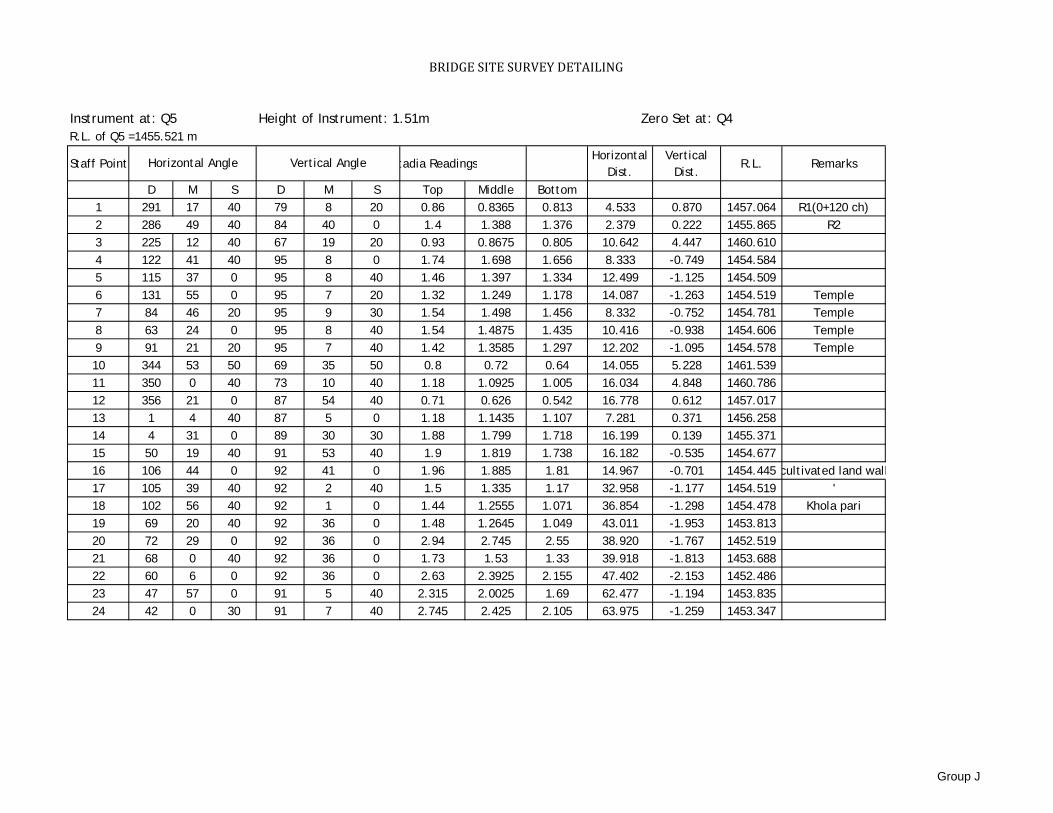
BRIDGE SITE SURVEY DETAILING
Instrument at: Q5 Zero Set at: Q4R.L. of Q5 =1455.521 m
Staff Point tadia ReadingsHorizontal
Dist.Vertical
Dist.R.L. Remarks
D M S D M S Top Middle Bottom1 291 17 40 79 8 20 0.86 0.8365 0.813 4.533 0.870 1457.064 R1(0+120 ch)2 286 49 40 84 40 0 1.4 1.388 1.376 2.379 0.222 1455.865 R23 225 12 40 67 19 20 0.93 0.8675 0.805 10.642 4.447 1460.6104 122 41 40 95 8 0 1.74 1.698 1.656 8.333 -0.749 1454.5845 115 37 0 95 8 40 1.46 1.397 1.334 12.499 -1.125 1454.5096 131 55 0 95 7 20 1.32 1.249 1.178 14.087 -1.263 1454.519 Temple7 84 46 20 95 9 30 1.54 1.498 1.456 8.332 -0.752 1454.781 Temple8 63 24 0 95 8 40 1.54 1.4875 1.435 10.416 -0.938 1454.606 Temple9 91 21 20 95 7 40 1.42 1.3585 1.297 12.202 -1.095 1454.578 Temple10 344 53 50 69 35 50 0.8 0.72 0.64 14.055 5.228 1461.53911 350 0 40 73 10 40 1.18 1.0925 1.005 16.034 4.848 1460.78612 356 21 0 87 54 40 0.71 0.626 0.542 16.778 0.612 1457.01713 1 4 40 87 5 0 1.18 1.1435 1.107 7.281 0.371 1456.25814 4 31 0 89 30 30 1.88 1.799 1.718 16.199 0.139 1455.37115 50 19 40 91 53 40 1.9 1.819 1.738 16.182 -0.535 1454.67716 106 44 0 92 41 0 1.96 1.885 1.81 14.967 -0.701 1454.445 cultivated land wall17 105 39 40 92 2 40 1.5 1.335 1.17 32.958 -1.177 1454.519 '18 102 56 40 92 1 0 1.44 1.2555 1.071 36.854 -1.298 1454.478 Khola pari19 69 20 40 92 36 0 1.48 1.2645 1.049 43.011 -1.953 1453.81320 72 29 0 92 36 0 2.94 2.745 2.55 38.920 -1.767 1452.51921 68 0 40 92 36 0 1.73 1.53 1.33 39.918 -1.813 1453.68822 60 6 0 92 36 0 2.63 2.3925 2.155 47.402 -2.153 1452.48623 47 57 0 91 5 40 2.315 2.0025 1.69 62.477 -1.194 1453.83524 42 0 30 91 7 40 2.745 2.425 2.105 63.975 -1.259 1453.347
Height of Instrument: 1.51m
Horizontal Angle Vertical Angle
Group J

BRIDGE SITE SURVEY DETAILING
Instrument at: Q6 Zero Set at: Q3R.L. of Q6 =1455.157 m
Staff Point Stadia Readings Horizontal
Dist.Vertical
Dist.R.L. Remarks
D M S D M S Top Middle Bottom1 52 17 0 96 4 0 2.74 2.675 2.61 12.855 -1.366 1452.536 (0+60Ch)2 13 22 20 96 2 40 2.74 2.676 2.612 12.658 -1.340 1452.561 '3 333 5 0 95 27 20 2.1 2.0875 2.075 2.477 -0.237 1454.253 '4 10 45 0 94 36 20 2.26 2.206 2.152 10.730 -0.864 1453.507 '5 253 3 20 94 43 0 1.44 1.425 1.41 2.980 -0.246 1454.906 '6 108 22 40 94 44 40 1.3 1.24 1.18 11.918 -0.989 1454.348 '7 82 47 0 94 44 20 2.14 2.0175 1.895 24.333 -2.017 1452.542 '8 122 31 40 94 44 0 1 0.9375 0.875 12.415 -1.028 1454.612 '9 88 40 0 94 38 40 1 0.88 0.76 23.843 -1.937 1453.760 '10 108 18 0 90 2 0 1.7 1.54 1.38 32.000 -0.019 1455.018 '11 92 1 0 90 46 20 3.7 3.51 3.32 37.993 -0.512 1452.555 '12 114 16 0 89 9 40 1.6 1.44 1.28 31.993 0.468 1455.605 '13 94 0 20 92 0 40 2.4 2.154 1.908 49.139 -1.726 1452.697 '14 97 16 0 92 4 0 1 0.751 0.502 49.735 -1.795 1454.031 '15 108 9 0 88 21 40 2.5 2.2225 1.945 55.455 1.587 1455.941 '16 112 5 20 88 18 20 2.6 2.32 2.04 55.951 1.655 1455.912 '
Height of Instrument: 1.42m
Horizontal Angle Vertical Angle
Group J
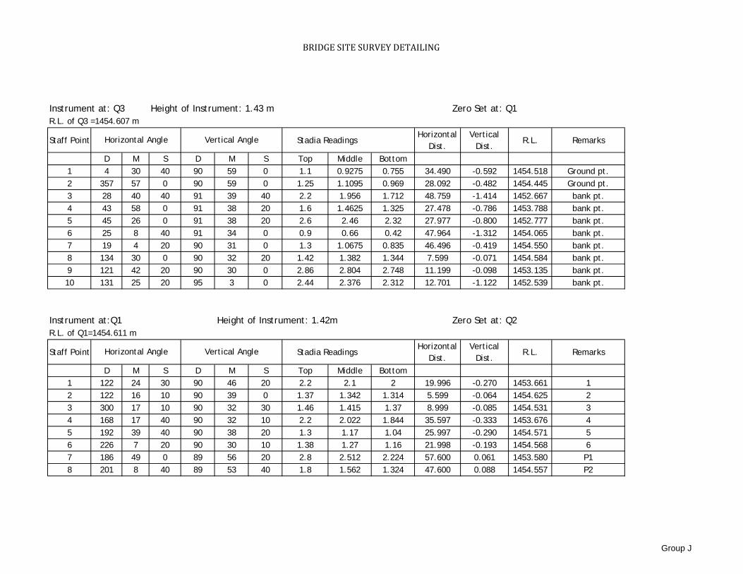
BRIDGE SITE SURVEY DETAILING
Instrument at: Q3 Zero Set at: Q1R.L. of Q3 =1454.607 m
Staff Point Stadia Readings Horizontal
Dist.Vertical
Dist.R.L. Remarks
D M S D M S Top Middle Bottom1 4 30 40 90 59 0 1.1 0.9275 0.755 34.490 -0.592 1454.518 Ground pt.2 357 57 0 90 59 0 1.25 1.1095 0.969 28.092 -0.482 1454.445 Ground pt.3 28 40 40 91 39 40 2.2 1.956 1.712 48.759 -1.414 1452.667 bank pt.4 43 58 0 91 38 20 1.6 1.4625 1.325 27.478 -0.786 1453.788 bank pt.5 45 26 0 91 38 20 2.6 2.46 2.32 27.977 -0.800 1452.777 bank pt.6 25 8 40 91 34 0 0.9 0.66 0.42 47.964 -1.312 1454.065 bank pt.7 19 4 20 90 31 0 1.3 1.0675 0.835 46.496 -0.419 1454.550 bank pt.8 134 30 0 90 32 20 1.42 1.382 1.344 7.599 -0.071 1454.584 bank pt.9 121 42 20 90 30 0 2.86 2.804 2.748 11.199 -0.098 1453.135 bank pt.10 131 25 20 95 3 0 2.44 2.376 2.312 12.701 -1.122 1452.539 bank pt.
Instrument at:Q1 Zero Set at: Q2R.L. of Q1=1454.611 m
Staff Point Stadia Readings Horizontal
Dist.Vertical
Dist.R.L. Remarks
D M S D M S Top Middle Bottom1 122 24 30 90 46 20 2.2 2.1 2 19.996 -0.270 1453.661 12 122 16 10 90 39 0 1.37 1.342 1.314 5.599 -0.064 1454.625 23 300 17 10 90 32 30 1.46 1.415 1.37 8.999 -0.085 1454.531 34 168 17 40 90 32 10 2.2 2.022 1.844 35.597 -0.333 1453.676 45 192 39 40 90 38 20 1.3 1.17 1.04 25.997 -0.290 1454.571 56 226 7 20 90 30 10 1.38 1.27 1.16 21.998 -0.193 1454.568 67 186 49 0 89 56 20 2.8 2.512 2.224 57.600 0.061 1453.580 P18 201 8 40 89 53 40 1.8 1.562 1.324 47.600 0.088 1454.557 P2
Vertical Angle
Horizontal Angle Vertical Angle
Height of Instrument: 1.42m
Height of Instrument: 1.43 m
Horizontal Angle
Group J
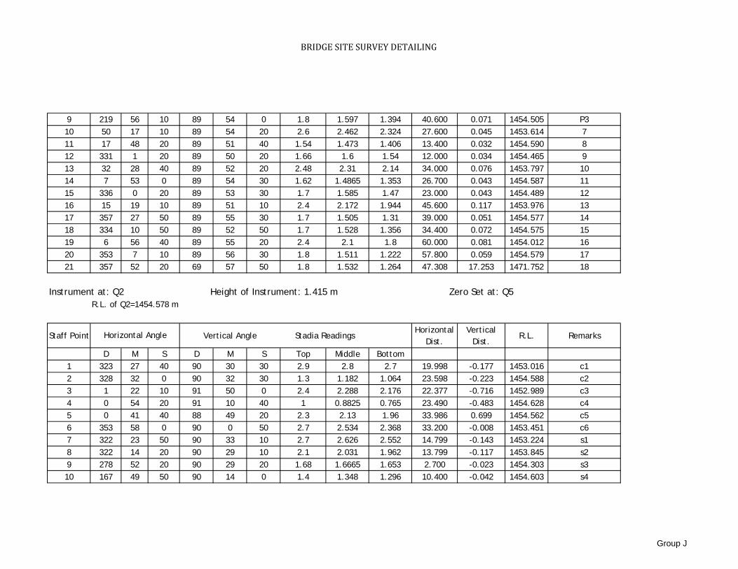
BRIDGE SITE SURVEY DETAILING
9 219 56 10 89 54 0 1.8 1.597 1.394 40.600 0.071 1454.505 P310 50 17 10 89 54 20 2.6 2.462 2.324 27.600 0.045 1453.614 711 17 48 20 89 51 40 1.54 1.473 1.406 13.400 0.032 1454.590 812 331 1 20 89 50 20 1.66 1.6 1.54 12.000 0.034 1454.465 913 32 28 40 89 52 20 2.48 2.31 2.14 34.000 0.076 1453.797 1014 7 53 0 89 54 30 1.62 1.4865 1.353 26.700 0.043 1454.587 1115 336 0 20 89 53 30 1.7 1.585 1.47 23.000 0.043 1454.489 1216 15 19 10 89 51 10 2.4 2.172 1.944 45.600 0.117 1453.976 1317 357 27 50 89 55 30 1.7 1.505 1.31 39.000 0.051 1454.577 1418 334 10 50 89 52 50 1.7 1.528 1.356 34.400 0.072 1454.575 1519 6 56 40 89 55 20 2.4 2.1 1.8 60.000 0.081 1454.012 1620 353 7 10 89 56 30 1.8 1.511 1.222 57.800 0.059 1454.579 1721 357 52 20 69 57 50 1.8 1.532 1.264 47.308 17.253 1471.752 18
Instrument at: Q2 Zero Set at: Q5R.L. of Q2=1454.578 m
Staff Point Vertical Angle Stadia Readings Horizontal
Dist.Vertical
Dist.R.L. Remarks
D M S D M S Top Middle Bottom1 323 27 40 90 30 30 2.9 2.8 2.7 19.998 -0.177 1453.016 c12 328 32 0 90 32 30 1.3 1.182 1.064 23.598 -0.223 1454.588 c23 1 22 10 91 50 0 2.4 2.288 2.176 22.377 -0.716 1452.989 c34 0 54 20 91 10 40 1 0.8825 0.765 23.490 -0.483 1454.628 c45 0 41 40 88 49 20 2.3 2.13 1.96 33.986 0.699 1454.562 c56 353 58 0 90 0 50 2.7 2.534 2.368 33.200 -0.008 1453.451 c67 322 23 50 90 33 10 2.7 2.626 2.552 14.799 -0.143 1453.224 s18 322 14 20 90 29 10 2.1 2.031 1.962 13.799 -0.117 1453.845 s29 278 52 20 90 29 20 1.68 1.6665 1.653 2.700 -0.023 1454.303 s310 167 49 50 90 14 0 1.4 1.348 1.296 10.400 -0.042 1454.603 s4
Horizontal Angle
Height of Instrument: 1.415 m
Group J
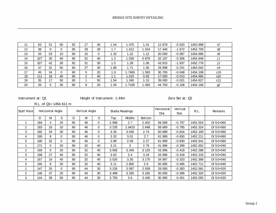
BRIDGE SITE SURVEY DETAILING
11 63 51 50 92 17 40 1.54 1.475 1.41 12.979 -0.520 1453.998 s712 38 9 0 95 28 30 1.7 1.612 1.524 17.440 -1.672 1452.709 s813 33 53 10 90 15 0 1.32 1.22 1.12 20.000 -0.087 1454.686 s914 327 30 40 90 32 40 1.2 1.039 0.878 32.197 -0.306 1454.648 j115 327 42 30 92 31 30 1.5 1.28 1.06 43.915 -1.937 1452.776 j216 47 31 50 90 27 40 1.86 1.71 1.56 29.998 -0.241 1454.042 c917 45 34 0 90 5 20 1.9 1.7465 1.593 30.700 -0.048 1454.199 c1018 111 18 40 90 2 40 1.1 1.015 0.93 17.000 -0.013 1454.965 s1019 35 17 50 90 1 50 1.54 1.345 1.15 39.000 -0.021 1454.627 c1120 26 0 30 90 8 20 1.94 1.7165 1.493 44.700 -0.108 1454.168 g2
Instrument at: Q1 Zero Set at: Q2
R.L. of Q1= 1454.611 m
Staff Point Stadia Readings Horizontal
Dist.Vertical
Dist.R.L. Remarks
D M S D M S Top Middle Bottom1 184 4 20 90 46 0 2.998 2.7 2.402 59.589 -0.797 1452.554 D/S 0+0602 183 16 10 90 46 0 3.235 2.9415 2.648 58.689 -0.785 1452.324 D/S 0+0603 182 34 30 90 46 0 3.35 3.045 2.74 60.989 -0.816 1452.190 D/S 0+0604 189 8 0 90 46 0 3.32 3.01 2.7 61.989 -0.830 1452.211 D/S 0+0605 180 32 0 90 46 0 2.89 2.58 2.27 61.989 -0.830 1452.641 D/S 0+0601 171 5 20 90 32 40 3.21 3 2.79 41.996 -0.399 1452.652 D/S 0+0402 169 0 20 90 32 40 3.565 3.345 3.125 43.996 -0.418 1452.288 D/S 0+0403 168 27 40 90 32 40 3.62 3.4 3.18 43.996 -0.418 1452.233 D/S 0+0404 167 16 40 90 32 40 3.525 3.35 3.175 34.997 -0.333 1452.368 D/S 0+0405 165 9 20 90 32 40 3.11 2.855 2.6 50.995 -0.485 1452.711 D/S 0+0401 147 25 0 90 44 30 3.235 3.087 2.939 29.595 -0.383 1452.581 D/S 0+0202 146 37 20 90 44 30 3.488 3.335 3.182 30.595 -0.396 1452.320 D/S 0+0203 144 39 50 90 44 30 3.755 3.6 3.445 30.995 -0.401 1452.050 D/S 0+020
Height of Instrument: 1.44m
Horizontal Angle Vertical Angle
Group J
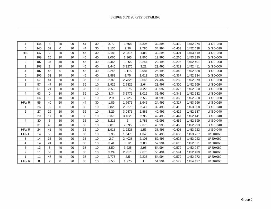
BRIDGE SITE SURVEY DETAILING
4 144 8 30 90 44 30 3.72 3.558 3.396 32.395 -0.419 1452.074 D/S 0+0205 140 52 0 90 44 30 3.135 2.96 2.785 34.994 -0.453 1452.638 D/S 0+020
HFL 147 2 30 90 45 30 2.183 2.0315 1.88 30.295 -0.401 1453.619 D/S 0+0201 109 25 20 90 45 40 2.065 1.965 1.865 19.996 -0.266 1453.820 D/S 0+0002 107 37 40 90 45 40 3.466 3.355 3.244 22.196 -0.295 1452.401 D/S 0+0003 108 2 30 90 45 40 3.445 3.3275 3.21 23.496 -0.312 1452.411 D/S 0+0004 107 46 0 90 45 40 3.246 3.115 2.984 26.195 -0.348 1452.588 D/S 0+0005 106 53 20 90 45 40 2.888 2.75 2.612 27.595 -0.367 1452.934 D/S 0+0001 57 41 50 90 36 10 2.92 2.7825 2.645 27.497 -0.289 1452.979 U/S 0+0202 57 47 30 90 36 10 2.925 2.7825 2.64 28.497 -0.300 1452.969 U/S 0+0203 61 21 30 90 36 10 3.53 3.375 3.22 30.997 -0.326 1452.350 U/S 0+0204 63 0 30 90 36 10 3.34 3.1775 3.015 32.496 -0.342 1452.532 U/S 0+0205 64 10 40 90 36 10 2.9 2.725 2.55 34.996 -0.368 1452.958 U/S 0+020
HFL/R 55 40 20 90 44 30 1.89 1.7675 1.645 24.496 -0.317 1453.966 U/S 0+0201 26 6 0 90 36 10 2.825 2.6275 2.43 39.496 -0.416 1453.008 U/S 0+0402 27 29 10 90 36 10 3.29 3.0875 2.885 40.496 -0.426 1452.537 U/S 0+0403 29 17 30 90 36 10 3.375 3.1625 2.95 42.495 -0.447 1452.441 U/S 0+0404 30 5 50 90 36 10 3.215 3 2.785 42.995 -0.452 1452.599 U/S 0+0405 31 43 40 90 36 10 2.815 2.595 2.375 43.995 -0.463 1452.993 U/S 0+040
HFL/R 24 41 40 90 36 10 1.915 1.7225 1.53 38.496 -0.405 1453.923 U/S 0+040HFL/L 14 55 40 90 36 10 1.95 1.6475 1.345 60.493 -0.636 1453.767 U/S0+060
5 14 33 20 90 36 10 2.7 2.4025 2.105 59.493 -0.626 1453.023 U/S0+0604 14 24 30 90 36 10 3.41 3.12 2.83 57.994 -0.610 1452.321 U/S0+0603 13 5 40 90 36 10 3.50 3.225 2.95 54.994 -0.579 1452.247 U/S0+0602 11 53 30 90 36 10 3.24 2.9575 2.675 56.494 -0.594 1452.499 U/S0+0601 11 47 40 90 36 10 2.775 2.5 2.225 54.994 -0.579 1452.972 U/S0+060
HFL/R 8 2 0 90 36 10 1.55 1.275 1 54.994 -0.579 1454.197 U/S0+060
Group J
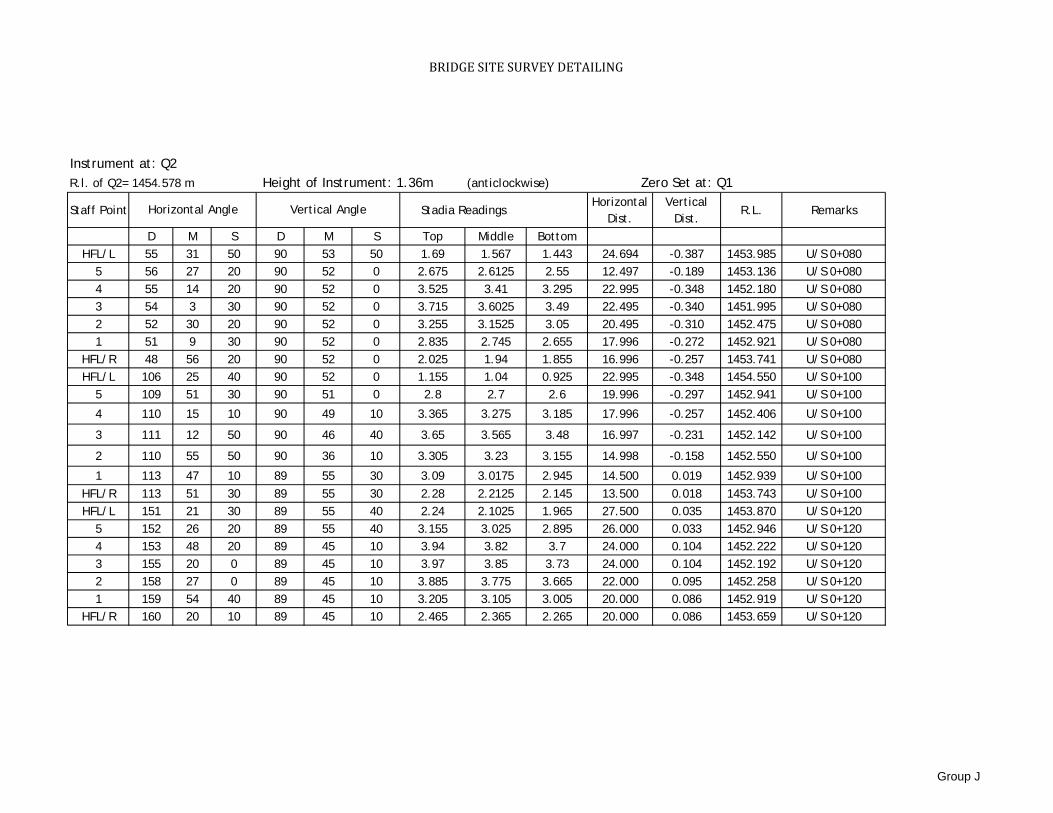
BRIDGE SITE SURVEY DETAILING
Instrument at: Q2R.l. of Q2= 1454.578 m Height of Instrument: 1.36m (anticlockwise) Zero Set at: Q1
Staff Point Stadia Readings Horizontal
Dist.Vertical
Dist.R.L. Remarks
D M S D M S Top Middle BottomHFL/L 55 31 50 90 53 50 1.69 1.567 1.443 24.694 -0.387 1453.985 U/S 0+080
5 56 27 20 90 52 0 2.675 2.6125 2.55 12.497 -0.189 1453.136 U/S 0+0804 55 14 20 90 52 0 3.525 3.41 3.295 22.995 -0.348 1452.180 U/S 0+0803 54 3 30 90 52 0 3.715 3.6025 3.49 22.495 -0.340 1451.995 U/S 0+0802 52 30 20 90 52 0 3.255 3.1525 3.05 20.495 -0.310 1452.475 U/S 0+0801 51 9 30 90 52 0 2.835 2.745 2.655 17.996 -0.272 1452.921 U/S 0+080
HFL/R 48 56 20 90 52 0 2.025 1.94 1.855 16.996 -0.257 1453.741 U/S 0+080HFL/L 106 25 40 90 52 0 1.155 1.04 0.925 22.995 -0.348 1454.550 U/S 0+100
5 109 51 30 90 51 0 2.8 2.7 2.6 19.996 -0.297 1452.941 U/S 0+100
4 110 15 10 90 49 10 3.365 3.275 3.185 17.996 -0.257 1452.406 U/S 0+100
3 111 12 50 90 46 40 3.65 3.565 3.48 16.997 -0.231 1452.142 U/S 0+100
2 110 55 50 90 36 10 3.305 3.23 3.155 14.998 -0.158 1452.550 U/S 0+100
1 113 47 10 89 55 30 3.09 3.0175 2.945 14.500 0.019 1452.939 U/S 0+100HFL/R 113 51 30 89 55 30 2.28 2.2125 2.145 13.500 0.018 1453.743 U/S 0+100HFL/L 151 21 30 89 55 40 2.24 2.1025 1.965 27.500 0.035 1453.870 U/S 0+120
5 152 26 20 89 55 40 3.155 3.025 2.895 26.000 0.033 1452.946 U/S 0+1204 153 48 20 89 45 10 3.94 3.82 3.7 24.000 0.104 1452.222 U/S 0+1203 155 20 0 89 45 10 3.97 3.85 3.73 24.000 0.104 1452.192 U/S 0+1202 158 27 0 89 45 10 3.885 3.775 3.665 22.000 0.095 1452.258 U/S 0+1201 159 54 40 89 45 10 3.205 3.105 3.005 20.000 0.086 1452.919 U/S 0+120
HFL/R 160 20 10 89 45 10 2.465 2.365 2.265 20.000 0.086 1453.659 U/S 0+120
Horizontal Angle Vertical Angle
Group J
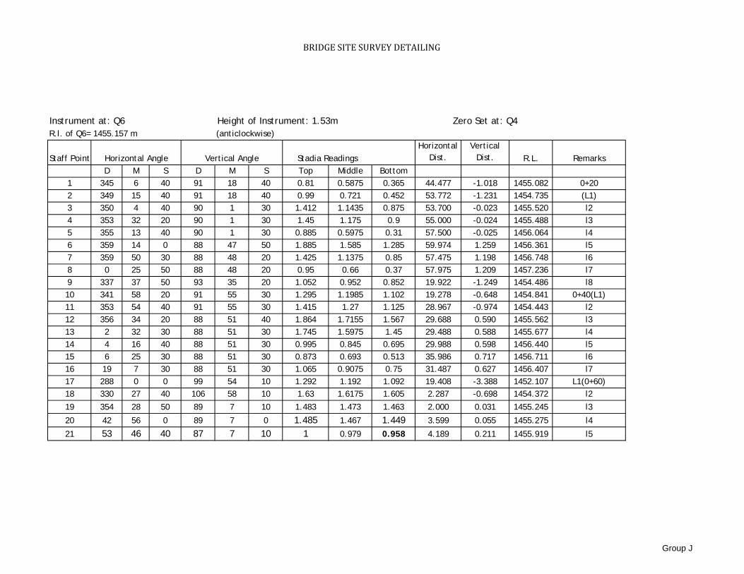
BRIDGE SITE SURVEY DETAILING
Instrument at: Q6 Zero Set at: Q4R.l. of Q6= 1455.157 m (anticlockwise)
Staff Point Stadia Readings Horizontal
Dist.Vertical
Dist. R.L. RemarksD M S D M S Top Middle Bottom
1 345 6 40 91 18 40 0.81 0.5875 0.365 44.477 -1.018 1455.082 0+202 349 15 40 91 18 40 0.99 0.721 0.452 53.772 -1.231 1454.735 (L1)3 350 4 40 90 1 30 1.412 1.1435 0.875 53.700 -0.023 1455.520 l24 353 32 20 90 1 30 1.45 1.175 0.9 55.000 -0.024 1455.488 l35 355 13 40 90 1 30 0.885 0.5975 0.31 57.500 -0.025 1456.064 l46 359 14 0 88 47 50 1.885 1.585 1.285 59.974 1.259 1456.361 l57 359 50 30 88 48 20 1.425 1.1375 0.85 57.475 1.198 1456.748 l68 0 25 50 88 48 20 0.95 0.66 0.37 57.975 1.209 1457.236 l79 337 37 50 93 35 20 1.052 0.952 0.852 19.922 -1.249 1454.486 l810 341 58 20 91 55 30 1.295 1.1985 1.102 19.278 -0.648 1454.841 0+40(L1)11 353 54 40 91 55 30 1.415 1.27 1.125 28.967 -0.974 1454.443 l212 356 34 20 88 51 40 1.864 1.7155 1.567 29.688 0.590 1455.562 l313 2 32 30 88 51 30 1.745 1.5975 1.45 29.488 0.588 1455.677 l414 4 16 40 88 51 30 0.995 0.845 0.695 29.988 0.598 1456.440 l515 6 25 30 88 51 30 0.873 0.693 0.513 35.986 0.717 1456.711 l616 19 7 30 88 51 30 1.065 0.9075 0.75 31.487 0.627 1456.407 l717 288 0 0 99 54 10 1.292 1.192 1.092 19.408 -3.388 1452.107 L1(0+60)18 330 27 40 106 58 10 1.63 1.6175 1.605 2.287 -0.698 1454.372 l2
19 354 28 50 89 7 10 1.483 1.473 1.463 2.000 0.031 1455.245 l3
20 42 56 0 89 7 0 1.485 1.467 1.449 3.599 0.055 1455.275 l4
21 53 46 40 87 7 10 1 0.979 0.958 4.189 0.211 1455.919 l5
Height of Instrument: 1.53m
Horizontal Angle Vertical Angle
Group J

BRIDGE SITE SURVEY DETAILING
Group J

BRIDGE SITE SURVEY DETAILING
Group J

BRIDGE SITE SURVEY DETAILING
Group J

BRIDGE SITE SURVEY DETAILING
Group J

BRIDGE SITE SURVEY DETAILING
l
Group J

BRIDGE SITE SURVEY DETAILING
Group J

BRIDGE SITE SURVEY DETAILING
Group J

BRIDGE SITE SURVEY DETAILING
Group J

BRIDGE SITE SURVEY DETAILING
Group J

BRIDGE SITE SURVEY DETAILING
Group J

BRIDGE SITE SURVEY DETAILING
Group J

BRIDGE SITE SURVEY DETAILING
Group J

BRIDGE SITE SURVEY DETAILING
Group J

BRIDGE SITE SURVEY DETAILING
Group J

BRIDGE SITE SURVEY DETAILING
Group J

BRIDGE SITE SURVEY DETAILING
Group J

BRIDGE SITE SURVEY DETAILING
Group J

BRIDGE SITE SURVEY DETAILING
Group J
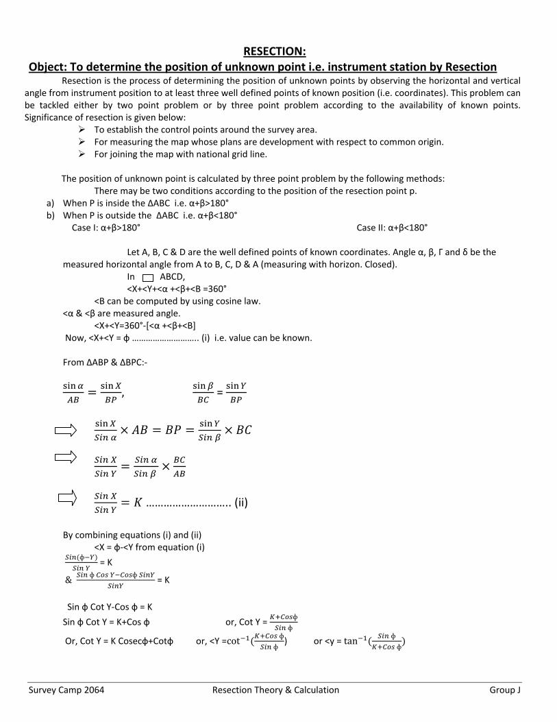
Survey Camp 2064 Resection Theory & Calculation Group J
RESECTION: Object: To determine the position of unknown point i.e. instrument station by Resection Resection is the process of determining the position of unknown points by observing the horizontal and vertical
angle from instrument position to at least three well defined points of known position (i.e. coordinates). This problem can be tackled either by two point problem or by three point problem according to the availability of known points. Significance of resection is given below:
To establish the control points around the survey area. For measuring the map whose plans are development with respect to common origin. For joining the map with national grid line.
The position of unknown point is calculated by three point problem by the following methods: There may be two conditions according to the position of the resection point p.
a) When P is inside the ∆ABC i.e. α+β>180° b) When P is outside the ∆ABC i.e. α+β<180°
Case I: α+β>180° Case II: α+β<180° Let A, B, C & D are the well defined points of known coordinates. Angle α, β, Γ and δ be the measured horizontal angle from A to B, C, D & A (measuring with horizon. Closed). In ABCD, <X+<Y+<α +<β+<B =360° <B can be computed by using cosine law. <α & <β are measured angle. <X+<Y=360°‐[<α +<β+<B] Now, <X+<Y = ф ……………………….. (i) i.e. value can be known. From ∆ABP & ∆BPC:‐
, =
……………………….. (ii)
By combining equations (i) and (ii) <X = ф‐<Y from equation (i)
ф
= K
& ф ф
= K
Sin ф Cot Y‐Cos ф = K
Sin ф Cot Y = K+Cos ф or, Cot Y = ф
ф
Or, Cot Y = K Cosecф+Cotф or, <Y =cot ф ф
) or <y = tan ф ф

Survey Camp 2064 Resection Theory & Calculation Group J
And, <X = ф ‐tan ф ф)
When angle <x & <y are computed then we can calculate the coordinate of unknown point P by using sine law for distance, Latitude & departure computation. Here, CP1, CP2 and W3 are three known points where coordinates is already computed and we have supposed these three points as S, D and H respectively. Let P be the unknown or instrument point whose coordinate is to be computed with the help of these known points. Here, we have the following data. From observation table: <JM4PW13 =46˚48’18.3’’=<α <W13PW12 =99˚36’33.3’’=<β <W12PJM4 =213˚35’8.34’’=<Г Here, α+β<180˚
FOR JM4W13: Length of JM4W13= 13 4 13 4
= 842.24 882.477 1014.587 991.863
= 40.237 22.724 =46.2103 m Easting of JM4W13 =Easting of W13‐ Easting of Jm4 =842.24‐882.477 =‐40.237 m Northing of JM4W13 = Northing of W13‐ Northing of JM4 =1014.587‐991.863 = 22.724 m
Bearing of JM4W13 =tan =tan ∆∆
= tan ..
=tan 1.77068 = N60˚32’39.28’’W =299˚27’20.72’’ (W.C.B.)
FOR W13W12:
Length of W13W12 = 814.175 842.24 1076.203 1014.587
= 28.065 61.616 =67.7065 M Easting of W13W12 = Easting of W12‐ Easting of W13 = 814.175‐842.24 =‐28.065 m Northing of W13W12 = Northing of W12‐ Northing of W13
Station Easting (M)X Northing(m)Y Altitude(m)
JM4 882.477 991.863 1331.179 W13 842.24 1014.587 1324.644 W12 814.175 1076.203 1327.774

Survey Camp 2064 Resection Theory & Calculation Group J
= 1076.203‐1014.587 = 61.616 m
Bearing of W13W12 =tan =tan ∆∆
= tan ..
=tan 0.45548 = N24˚29’18.34’’W =335˚30’41.66’’ (W.C.B.)
FOR W12JM4: Length of W12JM4 = 882.477 814.175 991.863 1076.203
= 68.302 84.34 =108.5283 m
Easting of W12JM4 = Easting of JM4‐ Easting of W12 = 882.477‐814.175 =68.302 m W12 (814.175, 1076.203) Northing of W12JM4 = Northing of JM4‐ Northing of W12 = 991.863‐1076.203 <Y = ‐84.34 m
Bearing of W12JM4 =tan =tan ∆∆
< β P(X, Y)
= tan ..
<W13 < α
=tan 0.80984 W13 = S39˚0’7.11’’E (842.24, 1014.587) <X =140˚59’52.89’’ (W.C.B.)
JM4 (882.477, 991.863) Now, <W13 = (360˚‐ Bearing of W13W12) + Bearing of W13JM4 = (360˚‐335˚30’41.66’’) + (299˚27’20.72’’‐180˚) =24˚29’18.34’’+119˚27’20.72’’ =143˚56’39.06’’ Now from JM4PW12W13, <X+<Y+<α+<β+<W13=360˚ And, <x+<y = 360˚‐<α+<β+<W13 =360˚‐(46˚48’18.3’’+99˚36’33.3’’+143˚56’39.06’’) =360˚‐290˚21’30.66’’ i.e.Φ =69˚38’29.34’’ Now we have, in ∆ PW12W13 &∆ PJM4W13, Using Sine law,
And
Or, PW13 = =
Or,
Or, K=
Or, K =˚ ’ . ’’˚ ’ . ’’
.
.
OR, k= 1.083361229 We have,
<Y = tan

Survey Camp 2064 Resection Theory & Calculation Group J
= tan ˚ ’ . ’’. ˚ ’ . ’’
= tan 0.65504 i.e. <Y = 33˚13’35.57’’ Now, <X = Φ‐<Y =69˚38’29.34’’‐33˚13’35.57’’ i.e. <X =36˚24’53.77’’ Now, from ∆PW12W13, Using Sine rule,
˚ ’ . ’’ ˚ ’ . ’ ˚ ’ . ’’
Or, . ˚ ’ . ’’ ˚ .
i.e. PW12 = 50.356 m
And, from ∆PW13JM4, Using Sine rule,
13 446˚48’18.3’’
4180 46˚48’18.3’’ 36˚24’53.77’’
Or, . ˚ ’ . ’’ ˚ .
i.e. PJM4 =62.943 m
Now, Bearing of JM4P =Bearing of W13JM4+<X+180˚ = (299˚27’20.72’’‐180˚) +36˚24’53.77’’+180˚ =335˚52’14.49’’ Easting of P w.r.t. JM4 =Easting of JM4 +Lsinθ =882.477 +62.943*sin (335˚52’14.49’’) = 856.746 m Northing of P w.r.t. JM4 = Northing of JM4+LCosθ =991.863+62.943*Cos (335˚52’14.49’’) =1049.3064 m I.e. the coordinate of B with respect to JM4 are: Easting(m) Northing(m) 856.746 1049.3064
Similarly, Easting of W13P = LW13p*Sinθ Now,
PW13 = 13 4
PW13 = ˚ ’ . ’’˚ ’ . ’’
46.2103 =37.6278 m
Bearing of W13P = bearing of W13JM4 – (180˚‐(46˚48’18.3’’+36˚24’53.77’’)) = (299˚27’20.72’’‐180˚)‐(96˚46’48’’) =22˚40’32.72’’ (W.C.B.) Easting of P w.r.t. W13 =Easting of W13 + L Sinθ = 842.24+37.6278*sin (22˚40’32.72’’) =856.746 m Northing of P w.r.t. W13 = Northing of W13+ LCosθ
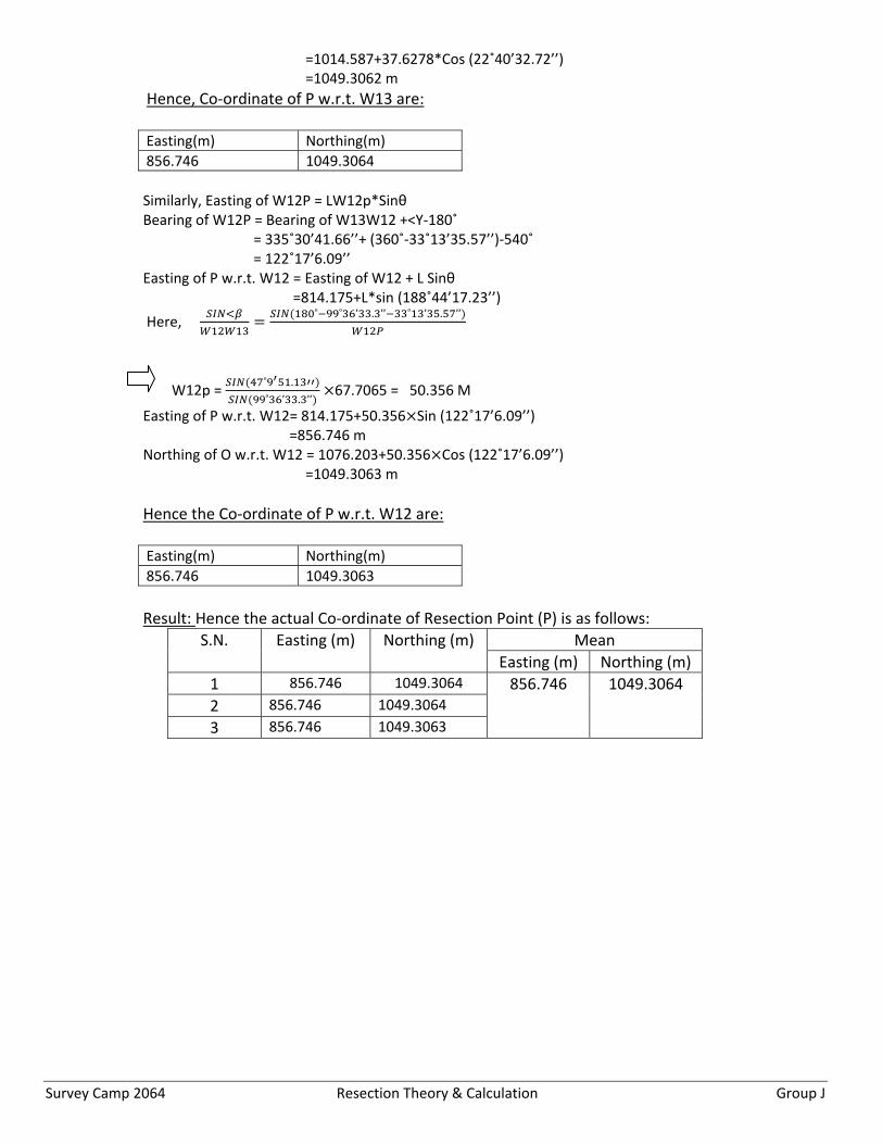
Survey Camp 2064 Resection Theory & Calculation Group J
=1014.587+37.6278*Cos (22˚40’32.72’’) =1049.3062 m Hence, Co‐ordinate of P w.r.t. W13 are: Easting(m) Northing(m) 856.746 1049.3064 Similarly, Easting of W12P = LW12p*Sinθ Bearing of W12P = Bearing of W13W12 +<Y‐180˚ = 335˚30’41.66’’+ (360˚‐33˚13’35.57’’)‐540˚ = 122˚17’6.09’’ Easting of P w.r.t. W12 = Easting of W12 + L Sinθ =814.175+L*sin (188˚44’17.23’’)
Here, ˚ ˚ ’ . ’’ ˚ ’ . ’’
W12p = ˚ .˚ ’ . ’’
67.7065 = 50.356 M
Easting of P w.r.t. W12= 814.175+50.356 Sin (122˚17’6.09’’) =856.746 m Northing of O w.r.t. W12 = 1076.203+50.356 Cos (122˚17’6.09’’) =1049.3063 m Hence the Co‐ordinate of P w.r.t. W12 are: Easting(m) Northing(m) 856.746 1049.3063 Result: Hence the actual Co‐ordinate of Resection Point (P) is as follows:
S.N. Easting (m) Northing (m) Mean Easting (m) Northing (m)
1 856.746 1049.3064 856.746 1049.3064 2 856.746 1049.3064
3 856.746 1049.3063
Related Documents