Surveillance Strategies for a Pursuer with Finite Sensor Range

Surveillance Strategies for a Pursuer with Finite Sensor Range

Rafael Murrieta-Cid∗, Teja Muppirala†, Alejandro Sarmiento†,Sourabh Bhattacharya† and Seth Hutchinson† †

[email protected] [email protected] [email protected]

[email protected] [email protected]

∗ Centro de Investigacion † University of Illinois

en Matematicas CIMAT at Urbana-Champaign

Guanajuato Mexico Urbana, IL 61801 USA

October 7, 2006

Abstract

This paper addresses the pursuit-evasion problem of maintaining surveillance by a pursuer of anevader in a world populated by polygonal obstacles. This requires the pursuer to plan collision-freemotions that honor distance constraints imposed by sensor capabilities, while avoiding occlusion ofthe evader by any obstacle. We extend the three-dimensional cellular decomposition of Schwartzand Sharir to represent the four-dimensional configuration space of the pursuer-evader system, andderive necessary conditions for surveillance (equivalently, sufficient conditions for escape) in termsof this new representation. We then give a game theoretic formulation of the problem, and usethis formulation to characterize optimal escape trajectories for the evader. We propose a shootingalgorithm that finds these trajectories using the minimum principle. Finally, noting the similaritiesbetween this surveillance problem and the problem of cooperative manipulation by two robots, wepresent several cooperation strategies that maximize system performance for cooperative motions.

Keywords: surveillance strategies, motion planning, pursuit-evasion

1 Introduction

In this paper, we consider the basic surveillance problem of planning motions for a pursuer such thatit maintains visibility of a moving evader in a known workspace containing obstacles. This is a variantof the traditional pursuit-evasion problem (discussed in Section 2) in which the pursuer has the goalof either catching or finding the evader. Our problem has application in several domains. In securityapplications, it may be desirable for a robot sentry to surveil a moving evader (either another robotor a human) as the evader moves through some sensitive area. In non-security applications, it maybe desirable for a robot to monitor the performance of another robot or of a human worker (e.g., amobile robot might follow a highway crew as it makes road repairs, monitoring the quality of the repair

∗Corresponding author†Early versions of this work have been presented at the IEEE Intl. Conf. on Robotics and Automation [25, 26] the

IEEE Intl. Conf. on Intelligent Robots and Systems [24] and the Intl. Conf. on Advanced Robotics [23]. This material isbased in part upon work supported by the National Science Foundation under Award Nos. CCR-0085917 and IIS-0083275.

1

work). Furthermore, as we will discuss below, our methods for planning surveillance strategies are alsoapplicable to situations in which robots cooperate, such as shared manipulation or maintaining robotformations.

For our problem, we assume that the evader is initially positioned within the pursuer’s field ofview, at a distance Linit from the pursuer. The pursuer’s goal is to maintain visibility of the evaderwhile maintaining a surveillance distance Lmin ≤ L ≤ Lmax, in which Lmin and Lmax are parametersdetermined by the capabilities of the sensor and by any pursuer safety concerns. This requires thepursuer to plan collision-free motions that prevent occlusion of the evader by obstacles in the workspace,while maintaining the surveillance distance in the interval [Lmin, Lmax]. We assume that the pursuer isprovided with a map of the workspace, and that the workspace is populated with polygonal obstacles.

In the case of a visibility based pursuit-evasion problem, it is pertinent to analyze the case ofbounded surveillance distance for the following reasons. First, commercially available sensors (laserand cameras) have upper and lower range limits. In particular, if the evader is farther from the pursuerthan a maximal sensor range then its location is unknown, and the surveillance is broken. The lowerbound on the surveillance distance may be due to sensor capabilities, but more likely it will deriveeither from safety concerns (e.g., if the evader has the ability to harm the pursuer) or from a desirefor the pursuer to remain undetected throughout the surveillance. Hence, if the evader is within thisminimal range, even if the pursuer can partially infer the location of the evader, the evader has alreadya great advantage: the pursuer may not be able to detect the evader, and furthermore, the evader hasthe ability to harm the pursuer.

A great deal of related research exists in the area of pursuit and evasion, much of it from thedynamics and control communities, and we review the most relevant of this in Section 2. This pastwork typically does not take into account constraints imposed on pursuer motion due to the existenceof obstacles in the workspace, or visibility constraints that arise due to occlusion. In this paper, wefocus on these often neglected geometric aspects of the problem.

In Section 3 we define the configuration space for our pursuer-evader system and derive an efficientcombinatoric representation for this configuration space. If the pursuer and evader are constrainedto remain separated by a fixed distance, the motion planning problem for the pursuer-evader systemis analogous to the problem of moving a rod in the plane. The basic problem of moving a rod inthe plane was solved by Schwartz and Sharir [31] using an elegant combinatoric representation ofthe set of free configurations. This representation can be extended to the case when the surveillancedistance is allowed to vary by noting that the qualitative structure of this representation changesonly at a finite set of critical values of the surveillance distance. Thus, we can represent the fullfour-dimensional configuration space of our pursuer-evader system by using a finite set of Schwartzand Sharir decompositions, provided we connect them appropriately. The description of this processconcludes Section 3.

The representation developed in Section 3 leads to a necessary condition for surveillance (symmetri-cally, a sufficient condition for the evader to escape), expressed in terms of the qualitative decompositionof the configuration space. In particular, in Section 4 we derive conditions for the existence of a surveil-lance strategy for the case of a pursuer with unbounded velocity. If no such strategy exists, then thereis no strategy for a pursuer with bounded velocity.

In Section 5, we formulate the surveillance problem using the language of noncooperative, dynamicgame theory. Here, we assume that the pursuer and evader have bounded velocities.

Conditions for escape are then formulated in terms of the time required by the evader to reach aparticular configuration, and the corresponding time required by the pursuer to reach a position fromwhich it can maintain surveillance.

For the case of bounded velocities, we solve the case corresponding to the following assumptions:The pursuer-evader system’s motion takes place in the free space up to the moment that the system

2

reaches a set of escapable configurations and the pursuer maintains a minimal surveillance distance.The formulation in Section 5 relies on the ability of the evader to plan optimal escape trajectories.

Therefore, in Section 6 we derive the optimal escape trajectories for the evader using Pontryagin’sminimum principle. In this section we propose a shooting algorithm to compute optimal escape tra-jectories, and show several results. For any such trajectory, it is straightforward for the pursuer todetermine the required motion to maintain surveillance. If the duration of this motion exceeds theduration of the optimal escape trajectory, the surveillance is broken.

The two robot pursuer-evader system becomes a team of two cooperating robots if the evader actsin concert with the pursuer. Therefore, in Section 7 we describe several cooperative motion strategies.These strategies could be used, for example, by two robots manipulating a rigid object. In this section,we consider leader-follower motions, in which the evader assumes the role of leader and the pursuerassumes the role of follower.

Finally, Section 8 provides conclusions and discusses future work.

2 Previous Work

Our surveillance problem is related to pursuit-evasion games. A great deal of research exists in thearea of pursuit and evasion, particularly in the area of dynamics and control in the free space (withoutobstacles) [9, 13, 3]. This work typically does not take into account constraints imposed on pursuermotion due to the existence of obstacles in the workspace, nor visibility constraints that arise due toocclusion.

Within the robotic planning community, several versions of the pursuit-evasion problem have beenconsidered. One such problem is that of finding an evader with one or more mobile pursuers thatsweep the environment so that the evader does not eventually sneak into an area that has been alreadyexplored. Exact [28, 32, 8, 18, 30] and probabilistic algorithms [33, 10, 15] have been proposed tosolve this problem. Another problem is to actually “catch” the evader, that is, to move to a contactconfiguration or closer than a given distance [13, 14].

These problems are related to, but not the same as ours. We assume that initially the pursuer canestablish visibility with the evader. Our problem consists of determining a pursuer motion strategyto always maintain that visibility. The problem of maintaining visibility of a moving evader has beentraditionally addressed with a combination of vision and control techniques [6, 12]. Pure controlapproaches, however, are local by nature, and do not take into account the global structure of theenvironment. Our interest is in deriving pursuer strategies that guarantee successful surveillance,taking into account both constraints on motion due to obstacles, and constraints on visibility due toocclusion.

Some previous work has addressed the motion planning problem for maintaining visibility of amoving evader. Game theory is proposed in [17] as a framework to formulate the tracking problemand an online algorithm is presented. In [4], an algorithm is presented that operates by maximizingthe probability of future visibility of the evader. This algorithm is also studied with more formalismin [17]. This technique was tested in a Nomad 200 mobile robot with good results.

The work in [7] presents an approach that takes into account the positioning uncertainty of therobot pursuer. Game theory is again proposed as a framework to formulate the tracking problem,and an approach is proposed that periodically commands the pursuer to move into a region that hasno localization uncertainty (a landmark region) in order to re-localize and better track the evaderafterward.

In [11], a technique is proposed to track an evader without the need of a global map. Instead, arange sensor is used to construct a local map of the environment, and a combinatoric algorithm is used

3

to compute a differential motion for the pursuer at each iteration.The approach presented in [22] computes a motion strategy by maximizing the shortest distance

to escape — the shortest distance the evader needs to move in order to escape the pursuer’s visibilityregion. In this work the evaders were assumed to move unpredictably, and the distribution of obstaclesin the workspace is assumed to be known in advance. This planner has been integrated and tested in arobot system that includes perceptual and control capabilities. The approach has also been extendedto maintain visibility of two evaders using two mobile pursuers.

Recently, some research has considered the problem of maintaining visibility of several evaders withmultiple robots. In [27] a method is proposed to accomplish this task in uncluttered environments.The objective is to minimize the total time in that evaders escape observation by some robot teammember. In [16] an approach is proposed to maintain visibility of several evaders using mobile andstatic sensors. A metric for measuring the degree of occlusion, based on the average mean free path ofa random line segment is used.

3 The Configuration Space for the Surveillance Problem

If we model the pursuer and evader as points in the plane, then our surveillance problem is very similarto the problem of planning the motion of a variable-length rod in the plane. The instantaneous distancebetween the pursuer and evader corresponds to the length of the rod, and occlusion of the evader by anobstacle corresponds to collision of the rod with an obstacle. To maintain surveillance, it is necessaryand sufficient that the line segment connecting the pursuer and evader does not intersect any obstaclein the environment. In addition to this occlusion constraint, a particular surveillance problem mayimpose bounds on the surveillance distance. For example, we may require that L ≤ Lmax if the sensorrange is bounded by Lmax. Further, there may be some minimum allowable surveillance distanceLmin. This minimum distance could be due to sensor capabilities, but it is more likely to derive fromsafety concerns (e.g., if the evader has the ability to harm the pursuer) or from the pursuer’s desire toremain undetected by the evader. We express this constraint by bounding the surveillance distance,Lmin ≤ L ≤ Lmax.

The problem of planning the motion of a fixed-length rod in the plane has been addressed in [31, 2].While this solution is not directly applicable to our surveillance problem, the representation introducedthere can be extended to the case of a rod with variable length, and this extended representationprovides the basis for the sufficient conditions for escape given in Section 4. In the remainder of thissection, we define the configuration space for our problem, briefly review the method of [31, 2], andshow how this representation can be extended to our surveillance problem.

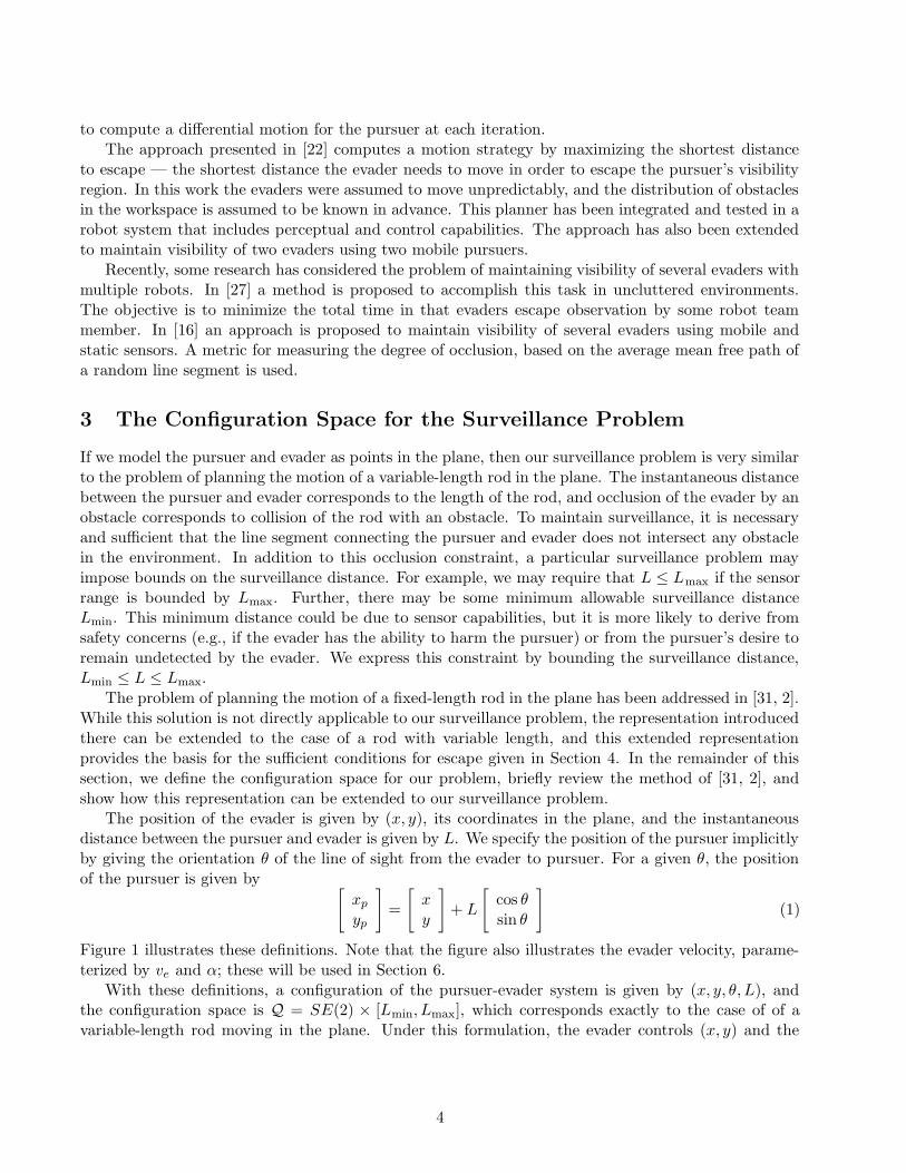
The position of the evader is given by (x, y), its coordinates in the plane, and the instantaneousdistance between the pursuer and evader is given by L. We specify the position of the pursuer implicitlyby giving the orientation θ of the line of sight from the evader to pursuer. For a given θ, the positionof the pursuer is given by

[

xp

yp

]

=

[

xy

]

+ L

[

cos θsin θ

]

(1)

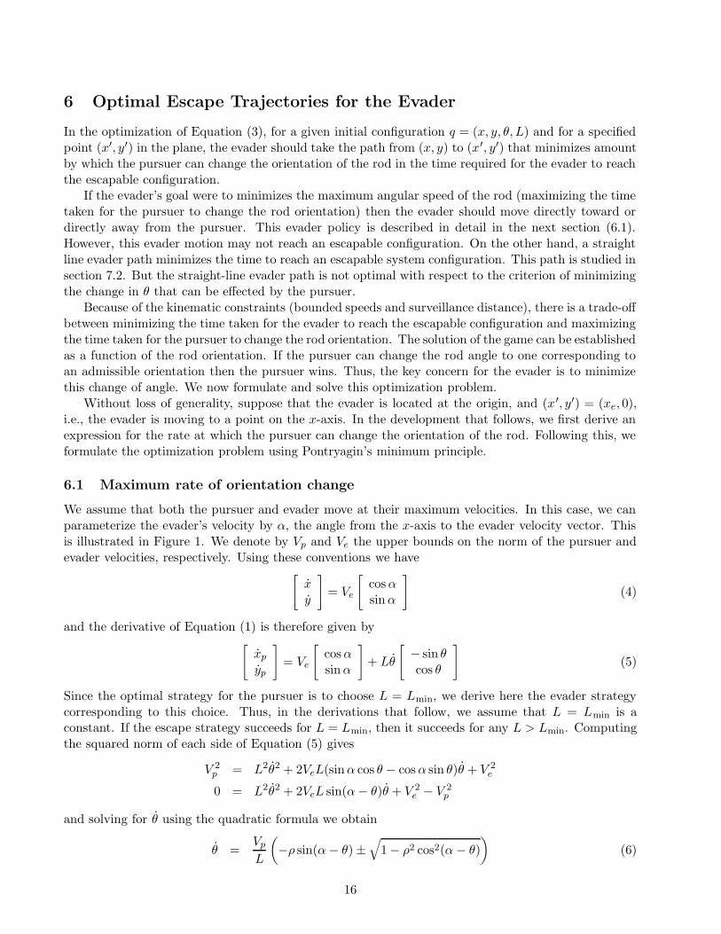
Figure 1 illustrates these definitions. Note that the figure also illustrates the evader velocity, parame-terized by ve and α; these will be used in Section 6.

With these definitions, a configuration of the pursuer-evader system is given by (x, y, θ, L), andthe configuration space is Q = SE(2) × [Lmin, Lmax], which corresponds exactly to the case of of avariable-length rod moving in the plane. Under this formulation, the evader controls (x, y) and the

4

E

P

P

θ

L

E

(x,y)

a) Basic Pursuer−Evader configuration

b) Occlusion

VE

α X−axis

��

��

Figure 1: The configuration variables for the pursuer-evader system

pursuer controls θ and L1. Thus, the task of the pursuer is to choose a trajectory θ(t), L(t) such thatthere is never a collision of the rod with an obstacle, and such that Lmin ≤ L(t) ≤ Lmax for all t.

This problems lends itself to an elegant combinatoric representation. To explain this representation,we first describe the cylindrical decomposition given in [31] for the case when L is fixed. Followingthis, we describe how the cylindrical decomposition can be extended to the case of variable L.

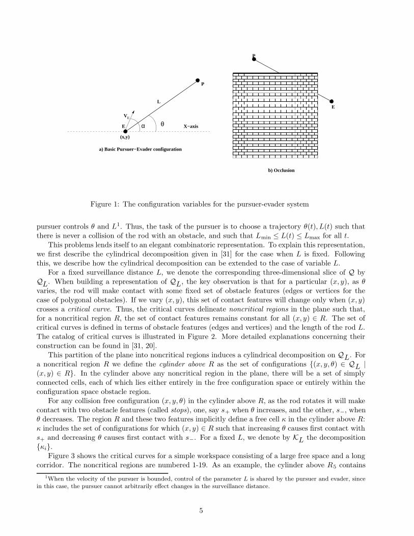
For a fixed surveillance distance L, we denote the corresponding three-dimensional slice of Q byQL. When building a representation of QL, the key observation is that for a particular (x, y), as θvaries, the rod will make contact with some fixed set of obstacle features (edges or vertices for thecase of polygonal obstacles). If we vary (x, y), this set of contact features will change only when (x, y)crosses a critical curve. Thus, the critical curves delineate noncritical regions in the plane such that,for a noncritical region R, the set of contact features remains constant for all (x, y) ∈ R. The set ofcritical curves is defined in terms of obstacle features (edges and vertices) and the length of the rod L.The catalog of critical curves is illustrated in Figure 2. More detailed explanations concerning theirconstruction can be found in [31, 20].

This partition of the plane into noncritical regions induces a cylindrical decomposition on QL. Fora noncritical region R we define the cylinder above R as the set of configurations {(x, y, θ) ∈ QL |(x, y) ∈ R}. In the cylinder above any noncritical region in the plane, there will be a set of simplyconnected cells, each of which lies either entirely in the free configuration space or entirely within theconfiguration space obstacle region.

For any collision free configuration (x, y, θ) in the cylinder above R, as the rod rotates it will makecontact with two obstacle features (called stops), one, say s+ when θ increases, and the other, s−, whenθ decreases. The region R and these two features implicitly define a free cell κ in the cylinder above R:κ includes the set of configurations for which (x, y) ∈ R such that increasing θ causes first contact withs+ and decreasing θ causes first contact with s−. For a fixed L, we denote by KL the decomposition{κi}.

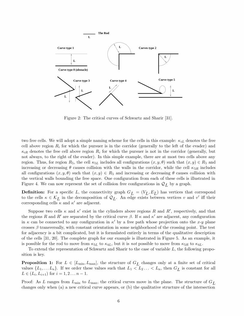
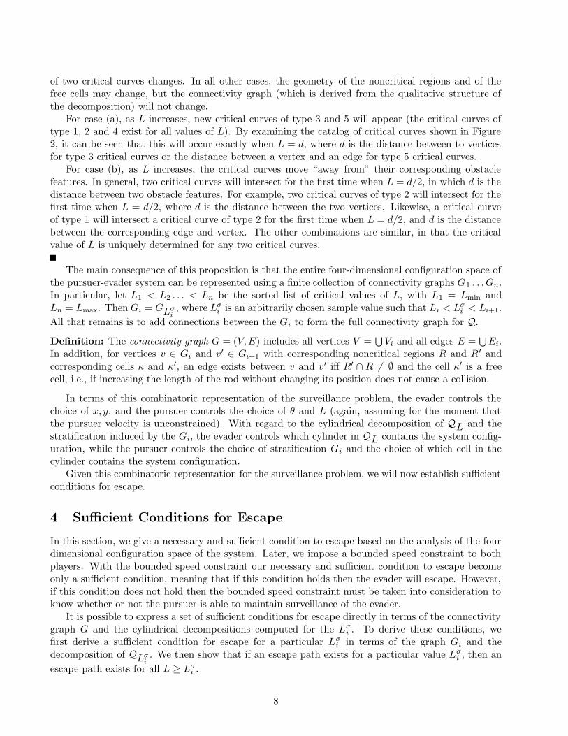
Figure 3 shows the critical curves for a simple workspace consisting of a large free space and a longcorridor. The noncritical regions are numbered 1-19. As an example, the cylinder above R5 contains

1When the velocity of the pursuer is bounded, control of the parameter L is shared by the pursuer and evader, sincein this case, the pursuer cannot arbitrarily effect changes in the surveillance distance.

5

Curve type 0 (obstacle)

Curve type 3

Curves type 2

Curve type 4 Curve type 5

Curve type 1

The RodL

L

L

L

LL

L

L

Figure 2: The critical curves of Schwartz and Sharir [31].

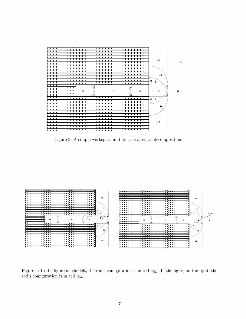
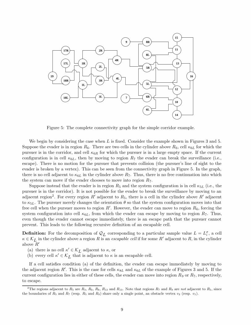
two free cells. We will adopt a simple naming scheme for the cells in this example: κiL denotes the freecell above region Ri for which the pursuer is in the corridor (generally to the left of the evader) andκiR denotes the free cell above region Ri for which the pursuer is not in the corridor (generally, butnot always, to the right of the evader). In this simple example, there are at most two cells above anyregion. Thus, for region R5, the cell κ5L includes all configurations (x, y, θ) such that (x, y) ∈ R5 andincreasing or decreasing θ causes collision with the walls in the corridor, while the cell κ5R includesall configurations (x, y, θ) such that (x, y) ∈ R5 and increasing or decreasing θ causes collision withthe vertical walls bounding the free space. One configuration from each of these cells is illustrated inFigure 4. We can now represent the set of collision free configurations in QL by a graph.

Definition: For a specific L, the connectivity graph GL = (VL,EL) has vertices that correspondto the cells κ ∈ KL in the decomposition of QL. An edge exists between vertices v and v ′ iff theircorresponding cells κ and κ′ are adjacent.

Suppose two cells κ and κ′ exist in the cylinders above regions R and R′, respectively, and thatthe regions R and R′ are separated by the critical curve β. If κ and κ′ are adjacent, any configurationin κ can be connected to any configuration in κ′ by a free path whose projection onto the x-y planecrosses β transversally, with constant orientation in some neighborhood of the crossing point. The testfor adjacency is a bit complicated, but it is formulated entirely in terms of the qualitative descriptionof the cells [31, 20]. The complete graph for our example is illustrated in Figure 5. As an example, itis possible for the rod to move from κ5L to κ4L, but it is not possible to move from κ5R to κ4L.

To extend the representation of Schwartz and Sharir to the case of variable L, the following propo-sition is key.

Proposition 1: For L ∈ [Lmin, Lmax], the structure of GL changes only at a finite set of criticalvalues {L1, . . . Ln}. If we order these values such that L1 < L2 . . . < Ln, then GL is constant for allL ∈ (Li, Li+1) for i = 1, 2 . . . n− 1.

Proof: As L ranges from Lmin to Lmax, the critical curves move in the plane. The structure of GLchanges only when (a) a new critical curve appears, or (b) the qualitative structure of the intersection

6

��

��

��

��

��

��

1

2

3

4 5

67

89

10

11

13

12

14

15

16

17

18

L

19

Figure 3: A simple workspace and its critical curve decomposition.

��

��

��

��

��

� � � � � � � � � � � � � � � � � � � � � � � � � � � � � � � � � � � � � � � � � � � � � � � � � � � � � � � � � � � � � � � � � � � � � � � � � � � � � � � � � � � � � � � � � � � � � � � � � � � � � � � � � � � � � � � � � � � � � � � � � � � � � � � � � � � � � � � � � � � � � � � � � � � � � � � � � � � � � � � � � � � � � � � � � � � � � � � � � � � � � � � � � � � � � � � � � � � � � � � � � � � � � � � � � � � � � � � � � � � � � � � � � � � � � � � � � � � � � � � � � � � � � � � � � � � � � � � � � � � � � � � � � � � � � � � � � � � � � � � � � � � � � � � � � � � � � � � � � � � � � � � � � � � � � � � � � � � � � � � � � � � � � � � � � � � � � � � � � � � � � � � � � � � � � � � � � � � � � � � � � � � � � � � � � � � � � � � � � � � � � � � � � � � � � � � � � � � �

1

2

3

4 5

67

89

10

11

13

12

14

15

16

17

18

19

��

��

��

��

��

��

1

2

3

4 5

67

89

10

11

13

12

14

15

16

17

18

19

EvaderPursuer

Pursuer

Evader

Figure 4: In the figure on the left, the rod’s configuration is in cell κ5L. In the figure on the right, therod’s configuration is in cell κ5R.

7

of two critical curves changes. In all other cases, the geometry of the noncritical regions and of thefree cells may change, but the connectivity graph (which is derived from the qualitative structure ofthe decomposition) will not change.

For case (a), as L increases, new critical curves of type 3 and 5 will appear (the critical curves oftype 1, 2 and 4 exist for all values of L). By examining the catalog of critical curves shown in Figure2, it can be seen that this will occur exactly when L = d, where d is the distance between to verticesfor type 3 critical curves or the distance between a vertex and an edge for type 5 critical curves.

For case (b), as L increases, the critical curves move “away from” their corresponding obstaclefeatures. In general, two critical curves will intersect for the first time when L = d/2, in which d is thedistance between two obstacle features. For example, two critical curves of type 2 will intersect for thefirst time when L = d/2, where d is the distance between the two vertices. Likewise, a critical curveof type 1 will intersect a critical curve of type 2 for the first time when L = d/2, and d is the distancebetween the corresponding edge and vertex. The other combinations are similar, in that the criticalvalue of L is uniquely determined for any two critical curves.

The main consequence of this proposition is that the entire four-dimensional configuration space ofthe pursuer-evader system can be represented using a finite collection of connectivity graphs G1 . . . Gn.In particular, let L1 < L2 . . . < Ln be the sorted list of critical values of L, with L1 = Lmin andLn = Lmax. Then Gi = GLσ

i, where Lσ

i is an arbitrarily chosen sample value such that Li < Lσi < Li+1.

All that remains is to add connections between the Gi to form the full connectivity graph for Q.

Definition: The connectivity graph G = (V,E) includes all vertices V =⋃

Vi and all edges E =⋃

Ei.In addition, for vertices v ∈ Gi and v′ ∈ Gi+1 with corresponding noncritical regions R and R′ andcorresponding cells κ and κ′, an edge exists between v and v′ iff R′ ∩ R 6= ∅ and the cell κ′ is a freecell, i.e., if increasing the length of the rod without changing its position does not cause a collision.

In terms of this combinatoric representation of the surveillance problem, the evader controls thechoice of x, y, and the pursuer controls the choice of θ and L (again, assuming for the moment thatthe pursuer velocity is unconstrained). With regard to the cylindrical decomposition of QL and thestratification induced by the Gi, the evader controls which cylinder in QL contains the system config-uration, while the pursuer controls the choice of stratification Gi and the choice of which cell in thecylinder contains the system configuration.

Given this combinatoric representation for the surveillance problem, we will now establish sufficientconditions for escape.

4 Sufficient Conditions for Escape

In this section, we give a necessary and sufficient condition to escape based on the analysis of the fourdimensional configuration space of the system. Later, we impose a bounded speed constraint to bothplayers. With the bounded speed constraint our necessary and sufficient condition to escape becomeonly a sufficient condition, meaning that if this condition holds then the evader will escape. However,if this condition does not hold then the bounded speed constraint must be taken into consideration toknow whether or not the pursuer is able to maintain surveillance of the evader.

It is possible to express a set of sufficient conditions for escape directly in terms of the connectivitygraph G and the cylindrical decompositions computed for the Lσ

i . To derive these conditions, wefirst derive a sufficient condition for escape for a particular Lσ

i in terms of the graph Gi and thedecomposition of QLσ

i. We then show that if an escape path exists for a particular value Lσ

i , then an

escape path exists for all L ≥ Lσi .

8

16

13

12

10

11

15

14

9 8R

8L

5R

2R

2L

3R

3L

1R

1L

19

17R

17L

18R

18L

6L

6R

5L

7

4L

4R

Figure 5: The complete connectivity graph for the simple corridor example.

We begin by considering the case when L is fixed. Consider the example shown in Figures 3 and 5.Suppose the evader is in region R6. There are two cells in the cylinder above R6, cell κ6L for which thepursuer is in the corridor, and cell κ6R for which the pursuer is in a large empty space. If the currentconfiguration is in cell κ6L, then by moving to region R7 the evader can break the surveillance (i.e.,escape). There is no motion for the pursuer that prevents collision (the pursuer’s line of sight to theevader is broken by a vertex). This can be seen from the connectivity graph in Figure 5. In the graph,there is no cell adjacent to κ6L in the cylinder above R7. Thus, there is no free continuation into whichthe system can move if the evader chooses to move into region R7.

Suppose instead that the evader is in region R5 and the system configuration is in cell κ5L (i.e., thepursuer is in the corridor). It is not possible for the evader to break the surveillance by moving to anadjacent region2. For every region R′ adjacent to R5, there is a cell in the cylinder above R′ adjacentto κ5L. The pursuer merely changes the orientation θ so that the system configuration moves into thatfree cell when the pursuer moves to region R′. However, the evader can move to region R6, forcing thesystem configuration into cell κ6L, from which the evader can escape by moving to region R7. Thus,even though the evader cannot escape immediately, there is an escape path that the pursuer cannotprevent. This leads to the following recursive definition of an escapable cell.

Definition: For the decomposition of QL corresponding to a particular sample value L = Lσi , a cell

κ ∈ KL in the cylinder above a region R is an escapable cell if for some R ′ adjacent to R, in the cylinderabove R′

(a) there is no cell κ′ ∈ KL adjacent to κ, or(b) every cell κ′ ∈ KL that is adjacent to κ is an escapable cell.

If a cell satisfies condition (a) of the definition, the evader can escape immediately by moving tothe adjacent region R′. This is the case for cells κ8L and κ6L of the example of Figures 3 and 5. If thecurrent configuration lies in either of these cells, the evader can move into region R9 or R7, respectively,to escape.

2The regions adjacent to R5 are R4, R6, R8, R12 and R13. Note that regions R7 and R9 are not adjacent to R5, sincethe boundaries of R5 and R7 (resp. R5 and R9) share only a single point, an obstacle vertex v2 (resp. v1).

9

If condition (b) of the definition is satisfied, the evader can escape by moving through a sequenceof adjacent regions, forcing the system configuration to move through a sequence of escapable cells,eventually reaching a cell that satisfies condition (a) of the definition. For the example of Figures 3and 5, if the system is in configuration κ1L, the evader can escape by following a path through regionsR3, R4, R5, R6 and R7. The pursuer has no choice but to follow, as the system configuration movesthrough cells κ3L, κ4L, κ5L, κ6L, and finally into collision when the evader moves into region R7. Thus,this sequence provides one guaranteed escape path for the evader.

By the definition above, the cell κ17L is an escapable cell that satisfies both conditions (a) and (b) ofthe definition. If the evader is in region R17 and moves into region R19, there is no motion possible forthe pursuer that maintains the surveillance distance L. This illustrates a second way for the evader to“escape” — it can force the pursuer into a position from which it cannot maintain surveillance distance,or, the evader can “force the pursuer into a corner.” Both of these cases are taken into account by ourdefinition of escapable cell.

As the above examples illustrate, for a fixed surveillance distance Lσi , the evader can escape if at any

time the system configuration enters an escapable cell. Thus, the pursuer must ensure that this doesnot occur. For the example of Figure 3, the pursuer strategy is simple: never enter the corridor, sincedoing so causes the system to enter some cell κiL, and no such cell exists in the reduced connectivitygraph. This leads to the following sufficient condition for escape.

Proposition 2: For a fixed surveillance distance Lσi , if there exists a region R such the cylinder above

R contains only escapable cells, the evader can force the system into an escapable cell by moving toregion R, from which there is a guaranteed escape path.

Proof: The proof is immediate from the recursive definition of escapable cells.

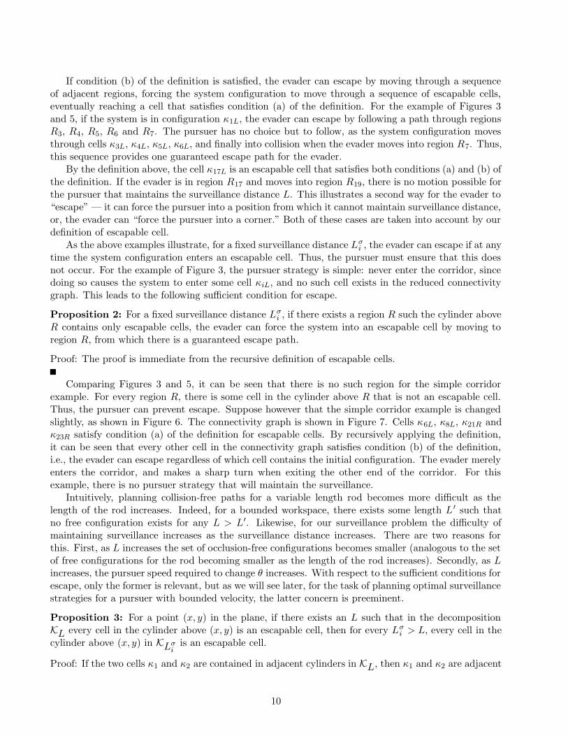
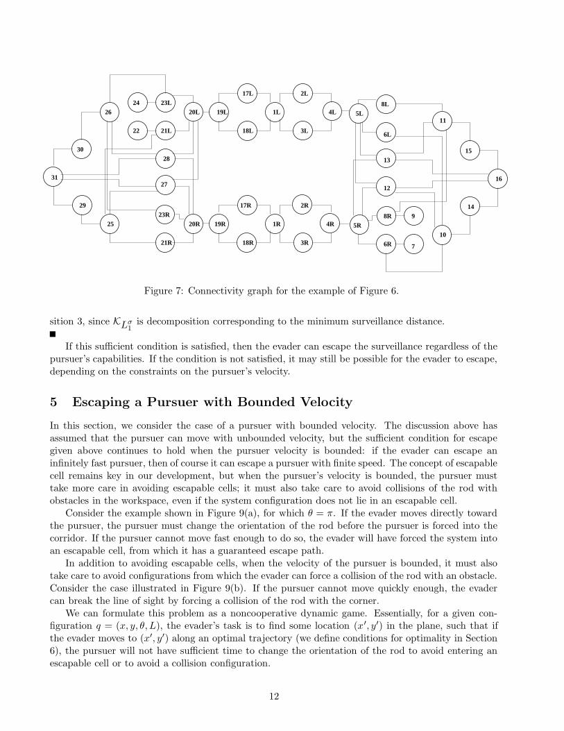
Comparing Figures 3 and 5, it can be seen that there is no such region for the simple corridorexample. For every region R, there is some cell in the cylinder above R that is not an escapable cell.Thus, the pursuer can prevent escape. Suppose however that the simple corridor example is changedslightly, as shown in Figure 6. The connectivity graph is shown in Figure 7. Cells κ6L, κ8L, κ21R andκ23R satisfy condition (a) of the definition for escapable cells. By recursively applying the definition,it can be seen that every other cell in the connectivity graph satisfies condition (b) of the definition,i.e., the evader can escape regardless of which cell contains the initial configuration. The evader merelyenters the corridor, and makes a sharp turn when exiting the other end of the corridor. For thisexample, there is no pursuer strategy that will maintain the surveillance.

Intuitively, planning collision-free paths for a variable length rod becomes more difficult as thelength of the rod increases. Indeed, for a bounded workspace, there exists some length L ′ such thatno free configuration exists for any L > L′. Likewise, for our surveillance problem the difficulty ofmaintaining surveillance increases as the surveillance distance increases. There are two reasons forthis. First, as L increases the set of occlusion-free configurations becomes smaller (analogous to the setof free configurations for the rod becoming smaller as the length of the rod increases). Secondly, as Lincreases, the pursuer speed required to change θ increases. With respect to the sufficient conditions forescape, only the former is relevant, but as we will see later, for the task of planning optimal surveillancestrategies for a pursuer with bounded velocity, the latter concern is preeminent.

Proposition 3: For a point (x, y) in the plane, if there exists an L such that in the decompositionKL every cell in the cylinder above (x, y) is an escapable cell, then for every Lσ

i > L, every cell in thecylinder above (x, y) in KLσ

iis an escapable cell.

Proof: If the two cells κ1 and κ2 are contained in adjacent cylinders in KL, then κ1 and κ2 are adjacent

10

��

��

��

��

1

2

3

4 5

67

89

10

11

13

12

14

15

16

17

18

19

2122

2324

20

25

26

27

28

29

30

31

L

Figure 6: A simple workspace in which a corridor connects two large empty spaces.

if and only if their ranges of free orientations overlap3. The cell κ1 is an escapable cell if no suchκ2 exists. For a particular (x, y), the range of free orientations is nonincreasing with increasing L.Therefore, if the projection onto the plane of κ1 ∈ KL contains (x, y), increasing the value of L willhave the effect of deforming κ1, and the resulting cell will also be an escapable cell, since the rangeof free orientations for the deformed cell can be no greater than for the original cell, and thus no newadjacencies can arise. Note that for some values of Lσ

i , the cell κ may actually split into multipledisconnected cells (each of which will have a range of free orientations that is no greater than the rangefor the original cell), and in this case, each of the resulting cells will be escapable cells.

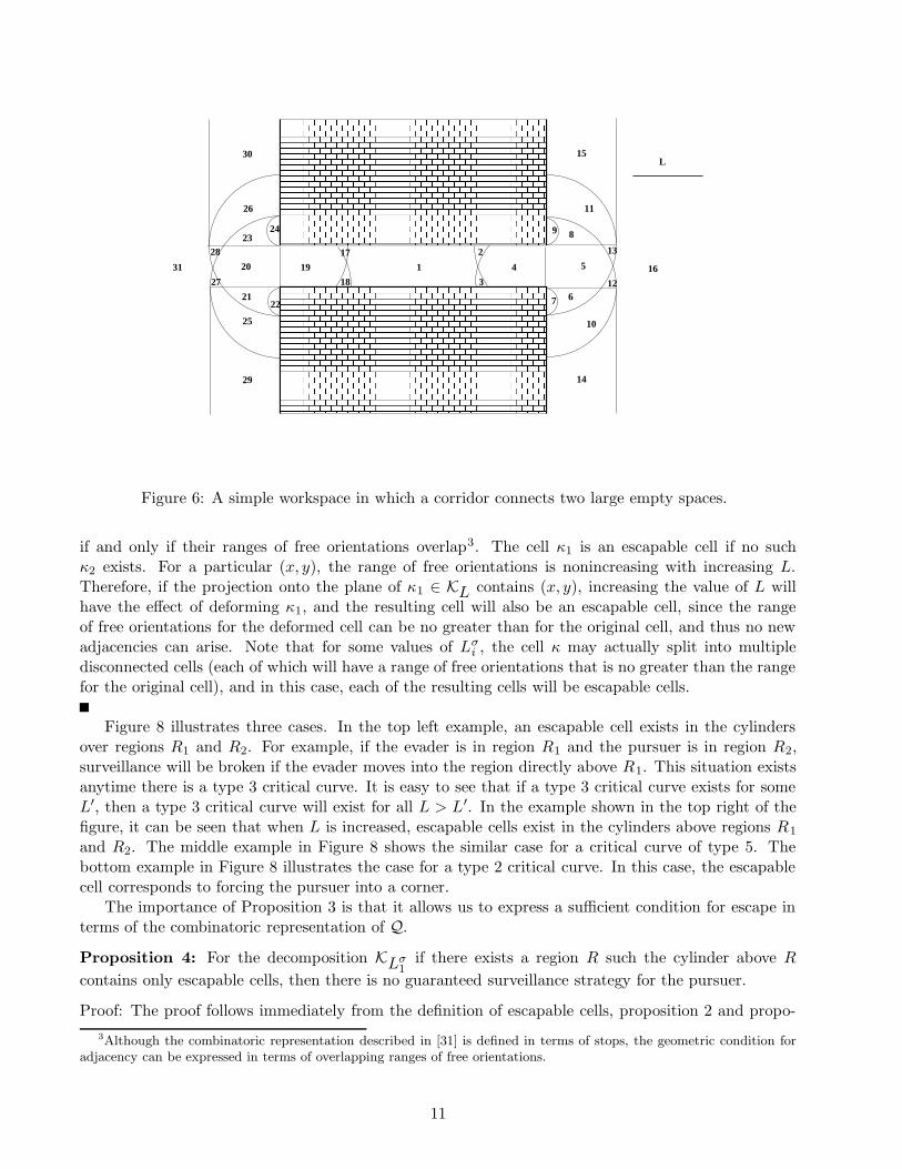
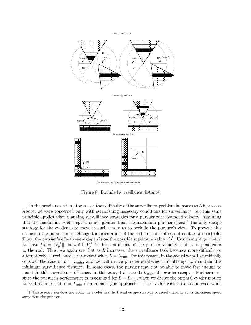
Figure 8 illustrates three cases. In the top left example, an escapable cell exists in the cylindersover regions R1 and R2. For example, if the evader is in region R1 and the pursuer is in region R2,surveillance will be broken if the evader moves into the region directly above R1. This situation existsanytime there is a type 3 critical curve. It is easy to see that if a type 3 critical curve exists for someL′, then a type 3 critical curve will exist for all L > L′. In the example shown in the top right of thefigure, it can be seen that when L is increased, escapable cells exist in the cylinders above regions R1

and R2. The middle example in Figure 8 shows the similar case for a critical curve of type 5. Thebottom example in Figure 8 illustrates the case for a type 2 critical curve. In this case, the escapablecell corresponds to forcing the pursuer into a corner.

The importance of Proposition 3 is that it allows us to express a sufficient condition for escape interms of the combinatoric representation of Q.

Proposition 4: For the decomposition KLσ1

if there exists a region R such the cylinder above R

contains only escapable cells, then there is no guaranteed surveillance strategy for the pursuer.

Proof: The proof follows immediately from the definition of escapable cells, proposition 2 and propo-

3Although the combinatoric representation described in [31] is defined in terms of stops, the geometric condition foradjacency can be expressed in terms of overlapping ranges of free orientations.

11

19L

17L

18L

1L

19R

17R

18R

1R

2L

3L

2R

3R

4L

4R

31

30

29

26

25

24

22

23L

21L

28

27

23R

21R

20L

20R

5L

5R

8L

6L

13

12

8R

6R

9

7

11

10

15

14

16

Figure 7: Connectivity graph for the example of Figure 6.

sition 3, since KLσ1

is decomposition corresponding to the minimum surveillance distance.

If this sufficient condition is satisfied, then the evader can escape the surveillance regardless of thepursuer’s capabilities. If the condition is not satisfied, it may still be possible for the evader to escape,depending on the constraints on the pursuer’s velocity.

5 Escaping a Pursuer with Bounded Velocity

In this section, we consider the case of a pursuer with bounded velocity. The discussion above hasassumed that the pursuer can move with unbounded velocity, but the sufficient condition for escapegiven above continues to hold when the pursuer velocity is bounded: if the evader can escape aninfinitely fast pursuer, then of course it can escape a pursuer with finite speed. The concept of escapablecell remains key in our development, but when the pursuer’s velocity is bounded, the pursuer musttake more care in avoiding escapable cells; it must also take care to avoid collisions of the rod withobstacles in the workspace, even if the system configuration does not lie in an escapable cell.

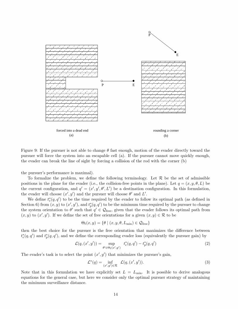
Consider the example shown in Figure 9(a), for which θ = π. If the evader moves directly towardthe pursuer, the pursuer must change the orientation of the rod before the pursuer is forced into thecorridor. If the pursuer cannot move fast enough to do so, the evader will have forced the system intoan escapable cell, from which it has a guaranteed escape path.

In addition to avoiding escapable cells, when the velocity of the pursuer is bounded, it must alsotake care to avoid configurations from which the evader can force a collision of the rod with an obstacle.Consider the case illustrated in Figure 9(b). If the pursuer cannot move quickly enough, the evadercan break the line of sight by forcing a collision of the rod with the corner.

We can formulate this problem as a noncooperative dynamic game. Essentially, for a given con-figuration q = (x, y, θ, L), the evader’s task is to find some location (x′, y′) in the plane, such that ifthe evader moves to (x′, y′) along an optimal trajectory (we define conditions for optimality in Section6), the pursuer will not have sufficient time to change the orientation of the rod to avoid entering anescapable cell or to avoid a collision configuration.

12

��

��

��

��

��

��

��

��

��

��

��

��

� � � � � � � � � � � � � � � � � � � � � � � � � � � � � � � � � � � � � � � � � � � � �

��

��

��

��

��

��

��

��

��

��

R1 R1

R2 Curve 3

Curve 2

Curve 3

Segment−Segment Case

Vertex−Segment Case

R1

R1

Curve 3

R2

Curve 3

R2R1Curve 5Curve 5

Curve 5 Curve 5

R1 R2

Curve 2

Regions associated to escapable cells are labeled

Vertex−Vertex Case

Figure 8: Bounded surveillance distance.

In the previous section, it was seen that difficulty of the surveillance problem increases as L increases.Above, we were concerned only with establishing necessary conditions for surveillance, but this sameprinciple applies when planning surveillance strategies for a pursuer with bounded velocity. Assumingthat the maximum evader speed is not greater than the maximum pursuer speed,4 the only escapestrategy for the evader is to move in such a way as to occlude the pursuer’s view. To prevent thisocclusion the pursuer must change the orientation of the rod so that it does not contact an obstacle.Thus, the pursuer’s effectiveness depends on the possible maximum value of θ. Using simple geometry,we have Lθ = ‖V ⊥

p ‖, in which V ⊥p is the component of the pursuer velocity that is perpendicular

to the rod. Thus, we again see that as L increases, the surveillance task becomes more difficult, oralternatively, surveillance is the easiest when L = Lmin. For this reason, in the sequel we will specificallyconsider the case of L = Lmin, and we will derive pursuer strategies that attempt to maintain thisminimum surveillance distance. In some cases, the pursuer may not be able to move fast enough tomaintain this surveillance distance. In this case, if L exceeds Lmax, the evader escapes. Furthermore,since the pursuer’s performance is maximized for L = Lmin, when we derive the optimal evader motionwe will assume that L = Lmin (a minimax type approach — the evader wishes to escape even when

4If this assumption does not hold, the evader has the trivial escape strategy of merely moving at its maximum speedaway from the pursuer

13

��

��

��

��

��

��

��

��

��

��

��

P E

rounding a corner(a) (b)

forced into a dead end

E

P

Figure 9: If the pursuer is not able to change θ fast enough, motion of the evader directly toward thepursuer will force the system into an escapable cell (a). If the pursuer cannot move quickly enough,the evader can break the line of sight by forcing a collision of the rod with the corner (b)

the pursuer’s performance is maximal).To formalize the problem, we define the following terminology. Let R be the set of admissible

positions in the plane for the evader (i.e., the collision-free points in the plane). Let q = (x, y, θ, L) bethe current configuration, and q′ = (x′, y′, θ′, L′) be a destination configuration. In this formulation,the evader will choose (x′, y′) and the pursuer will choose θ′ and L′.

We define t∗e(q, q′) to be the time required by the evader to follow its optimal path (as defined in

Section 6) from (x, y) to (x′, y′), and t∗p(q, q′) to be the minimum time required by the pursuer to change

the system orientation to θ′ such that q′ ∈ Qfree, given that the evader follows its optimal path from(x, y) to (x′, y′). If we define the set of free orientations for a given (x, y) ∈ R to be

Θf(x, y) = {θ | (x, y, θ, Lmin) ∈ Qfree}

then the best choice for the pursuer is the free orientation that maximizes the difference betweent∗e(q, q

′) and t∗p(q, q′), and we define the corresponding evader loss (equivalently the pursuer gain) by

L(q, (x′, y′)) = supθ′∈Θf(x′,y′)

t∗e(q, q′)− t∗p(q, q

′) (2)

The evader’s task is to select the point (x′, y′) that minimizes the pursuer’s gain,

L∗(q) = inf(x′,y′)∈R

L(q, (x′, y′)). (3)

Note that in this formulation we have explicitly set L = Lmin. It is possible to derive analogousequations for the general case, but here we consider only the optimal pursuer strategy of maintainingthe minimum surveillance distance.

14

With this formulation, the evader escapes when L∗(q) < 0. This leads to the bounded-velocityanalog of an escapable cell.

Definition: A configuration q is an escapable configuration if L∗(q) < 0.

There are several limiting cases. If both (x, y) and (x′, y′) lie in the same region R, and R is aregion with no stops (i.e., the rod can rotate freely), then t∗p(q, q

′) = 0; the pursuer need make noeffort to change the system orientation. If there is no collision free path for (x ′, y′), then we definet∗p(q, q

′) = ∞. For the case of a pursuer with unbounded velocity, we have t∗p(q, q′) = 0 when q does

not lie in an escapable cell, and t∗p(q, q′) = ∞ when q lies in an escapable cell and the evader follows

a guaranteed escape path. In this case a configuration that lies in an escapable cell is trivially anescapable configuration.

For a given evader position (x, y), L∗(q) depends not only on x and y, but also on the value of θ.This leads to the following definitions.

Definition: For a given evader position in the plane, the set of admissible orientations for the rod isgiven by

Θadm(x, y) = {θ | q = (x, y, θ, Lmin), L∗(q) > 0}

and a configuration q = (x, y, θ, Lmin) is said to be an admissible configuration if θ ∈ Θadm(x, y). Wewill denote by Qadm the set of admissible configurations. This leads to our sufficient condition forescape when the pursuer has bounded velocity.

Proposition 5: If there exists a point (x, y) ∈ R such that Θadm(x, y) = ∅, then there is an escapepath for the evader originating at (x, y).

If the condition of the proposition is not satisfied, then it is the task of the pursuer to keep theconfiguration of the rod in Qadm by choosing θ ∈ Θadm(x, y) as the evader traces a path in the plane.In the next section, we describe the pursuer policy to keep θ ∈ Θadm(x, y).

We solve the specific portion of the pursuit evasion game corresponding to the following assumptions:The rod’s motion takes place in the free space up to the moment that the system reaches an escapableconfiguration, which corresponds to a contact with either an obstacle or an escapable cell. The pursuermaintains a minimal surveillance distance, and the set of escapable configurations is bounded by criticalcurves.

It is possible to formulate and solve this part of the whole game, even if the global trajectories ofboth evader and pursuer are unknown in advance. In other words, it is possible to deduce the localmotion policies of both pursuer and evader and the required final rod orientation.

When the pursuer maintains the minimum surveillance distance, its trajectory can be decomposedinto two components: one that is equal to the evader velocity and one that is perpendicular to the rod.This is true regardless of the evader’s trajectory, and it does not require any cooperation on the partof the evader (i.e., it applies to the case of an antagonistic evader). In this case, the evader trajectorycan influence the rate of change in θ, but not the initial and final orientations. Thus, the policy for thepursuer to change the rod from an initial orientation to a final one (avoiding an escapable configuration)will be the same regardless of the actual evader trajectory.

Since we know in advance both the map and the maximum velocities of the evader and the pursuer,then the escapable configurations are also known. If there is more than one set of escapable config-urations then the evader can choose the optimal one with respect to a given criterion related to thecapabilities of the pursuer. Thus, knowledge of the optimal final rod orientation can be deduced fromthe map.

The task of the evader is to find the optimal motion strategy to escape. In the section 6, we describethe proposed optimality criterion. We also explain the validity of this optimization criterion.

15

6 Optimal Escape Trajectories for the Evader

In the optimization of Equation (3), for a given initial configuration q = (x, y, θ, L) and for a specifiedpoint (x′, y′) in the plane, the evader should take the path from (x, y) to (x′, y′) that minimizes amountby which the pursuer can change the orientation of the rod in the time required for the evader to reachthe escapable configuration.

If the evader’s goal were to minimizes the maximum angular speed of the rod (maximizing the timetaken for the pursuer to change the rod orientation) then the evader should move directly toward ordirectly away from the pursuer. This evader policy is described in detail in the next section (6.1).However, this evader motion may not reach an escapable configuration. On the other hand, a straightline evader path minimizes the time to reach an escapable system configuration. This path is studied insection 7.2. But the straight-line evader path is not optimal with respect to the criterion of minimizingthe change in θ that can be effected by the pursuer.

Because of the kinematic constraints (bounded speeds and surveillance distance), there is a trade-offbetween minimizing the time taken for the evader to reach the escapable configuration and maximizingthe time taken for the pursuer to change the rod orientation. The solution of the game can be establishedas a function of the rod orientation. If the pursuer can change the rod angle to one corresponding toan admissible orientation then the pursuer wins. Thus, the key concern for the evader is to minimizethis change of angle. We now formulate and solve this optimization problem.

Without loss of generality, suppose that the evader is located at the origin, and (x ′, y′) = (xe, 0),i.e., the evader is moving to a point on the x-axis. In the development that follows, we first derive anexpression for the rate at which the pursuer can change the orientation of the rod. Following this, weformulate the optimization problem using Pontryagin’s minimum principle.

6.1 Maximum rate of orientation change

We assume that both the pursuer and evader move at their maximum velocities. In this case, we canparameterize the evader’s velocity by α, the angle from the x-axis to the evader velocity vector. Thisis illustrated in Figure 1. We denote by Vp and Ve the upper bounds on the norm of the pursuer andevader velocities, respectively. Using these conventions we have

[

xy

]

= Ve

[

cos αsinα

]

(4)

and the derivative of Equation (1) is therefore given by[

xp

yp

]

= Ve

[

cos αsinα

]

+ Lθ

[

− sin θcos θ

]

(5)

Since the optimal strategy for the pursuer is to choose L = Lmin, we derive here the evader strategycorresponding to this choice. Thus, in the derivations that follow, we assume that L = Lmin is aconstant. If the escape strategy succeeds for L = Lmin, then it succeeds for any L > Lmin. Computingthe squared norm of each side of Equation (5) gives

V 2p = L2θ2 + 2VeL(sinα cos θ − cos α sin θ)θ + V 2

e

0 = L2θ2 + 2VeL sin(α− θ)θ + V 2e − V 2

p

and solving for θ using the quadratic formula we obtain

θ =Vp

L

(

−ρ sin(α− θ)±√

1− ρ2 cos2(α− θ)

)

(6)

16

in which 0 < ρ ≤ 1 is the ratio of Ve to Vp. Note, if ρ > 1, it is trivial for the evader to escape.To simplify notation, define

θ+ =Vp

L

(

−ρ sin(α− θ) +√

1− ρ2 cos2(α− θ)

)

θ− =Vp

L

(

−ρ sin(α− θ)−√

1− ρ2 cos2(α− θ)

)

The decision of whether to use θ+ or θ− is made by the pursuer, based on whether the pursuerwishes to maximize | θ |, to have θ < 0, or to have θ > 0. Since 0 < ρ ≤ 1,

| ρ sinφ |≤√

1− ρ2 cos2 φ

and therefore θ+ > 0 and θ− < 0.The magnitude of the angular change | θ | is maximized by choosing θ+ when sin(α − θ) < 0, and

choosing θ− when sin(α− θ) > 0. When sin(α− θ) = 0, either choice will yield

| θ |= +Vp

L

√

1− ρ2 cos2(α− θ)

The maximum angular speed is then given by

max | θ |=

{

| θ− | 0 ≤ α− θ ≤ π

θ+ π ≤ α− θ ≤ 2π

In the interval 0 < α−θ < π, the function | θ− | is concave. Likewise, in the interval π < α−θ < 2π,the function θ+ is concave. Thus, the minimum is achieved at the transition point, where | θ− |= θ+,and where the derivative of max | θ | is discontinuous, i.e., for (α − θ) = kπ. Therefore, if the evaderwishes to choose a velocity that minimizes the maximum angular speed of the rod, the evader shouldmove directly toward or directly away from the pursuer.

6.2 Formulating the optimal control problem

In formulating the optimal control problem, it is convenient to let x be the independent variable(instead of time t) and to parameterize the control α by x, since the evader will move from the pointx = 0 to the point x′ = xe. It is clear that the projection of the evader position onto the x-axis willbe monotonically increasing, so this is a reasonable choice for a parameterization of the problem. Thisleads to a modified system description in which the state of the rod is given by ζ = (y, θ), and thesystem equation is given by

d

dxζ = f(ζ, α)

The time derivatives for x and y are given by

dx

dt= Ve cos α

dy

dt= Ve sinα

With respect to the independent variable x, the state equations are then given by

dy

dx=

dy

dt

(

dx

dt

)−1

= tan α = f1(ζ, α)

17

dθ

dx=

dθ

dt

(

dx

dt

)−1

=−ρ sin(α− θ)±

√

1− ρ2 cos2(α− θ)

Lρ cos α= f2(ζ, α)

In the remainder of this section, to simplify notation, we will use θ, λ, and ζ, to denote the derivativesof θ, λ and ζ with respect to x rather than with respect to time. Further, in this section we will onlysolve the problem for the case of θ = θ+. The case for θ = θ− is analogous.

To minimize the angle by which the pursuer can change the orientation of the rod, we use the costfunction

J =

∫ xe

0

dθ

dxdx

=

∫ xe

0f2(ζ, α)dx

Thus, we seek the control input α that minimizes J , subject to the system equation ζ = f(ζ, α),and subject to the boundary conditions

θ(0) = θ, y(0) = y(xe) = 0

To solve this optimization problem, we use the minimum principle and solve the resulting equationsnumerically using a shooting method.

The system Hamiltonian is given by

H(ζ, α, x) =dθ

dx+ λ1(x)f1(ζ, α) + λ2(x)f2(ζ, α)

= λ1f1(ζ, α) + (1 + λ2)f2(ζ, α)

= λ1 tanα +

(1 + λ2)−ρ sin(α− θ) +

√

1− ρ2 cos2(α− θ)

Lρ cos α

in which λi(x) are the Lagrange multipliers, which are a function of the independent variable x.The adjoint equation for λ1 is given by

λ1 = −∂

∂yH = 0

which implies that λ1 is a constant. This allows us to write the Hamiltonian as

H(ζ, α, x) = K tanα

+(1 + λ2)−ρ sin(α− θ) +

√

1− ρ2 cos2(α− θ)

Lρ cos α

The adjoint equation for λ2 is given by

λ2 = −∂

∂θH

= −(1 + λ2)cos(α − θ)

L cos α

(

1−ρ sin(α− θ)

√

1− ρ2 cos2(α− θ)

)

18

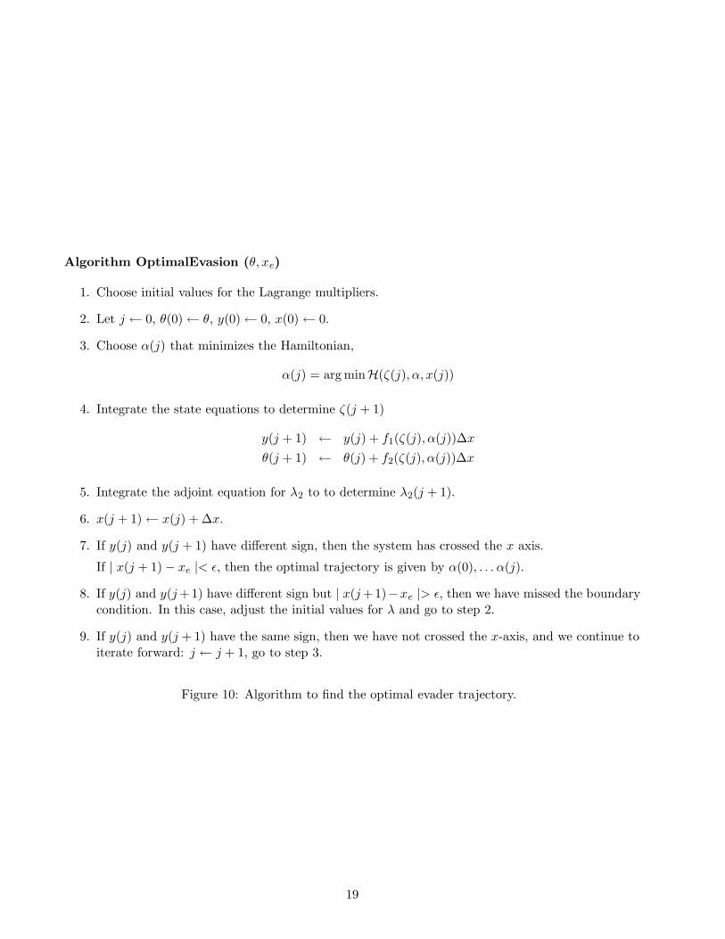
Algorithm OptimalEvasion (θ, xe)

1. Choose initial values for the Lagrange multipliers.

2. Let j ← 0, θ(0)← θ, y(0)← 0, x(0)← 0.

3. Choose α(j) that minimizes the Hamiltonian,

α(j) = arg minH(ζ(j), α, x(j))

4. Integrate the state equations to determine ζ(j + 1)

y(j + 1) ← y(j) + f1(ζ(j), α(j))∆x

θ(j + 1) ← θ(j) + f2(ζ(j), α(j))∆x

5. Integrate the adjoint equation for λ2 to to determine λ2(j + 1).

6. x(j + 1)← x(j) + ∆x.

7. If y(j) and y(j + 1) have different sign, then the system has crossed the x axis.

If | x(j + 1)− xe |< ε, then the optimal trajectory is given by α(0), . . . α(j).

8. If y(j) and y(j +1) have different sign but | x(j +1)−xe |> ε, then we have missed the boundarycondition. In this case, adjust the initial values for λ and go to step 2.

9. If y(j) and y(j + 1) have the same sign, then we have not crossed the x-axis, and we continue toiterate forward: j ← j + 1, go to step 3.

Figure 10: Algorithm to find the optimal evader trajectory.

19

(a) (b)

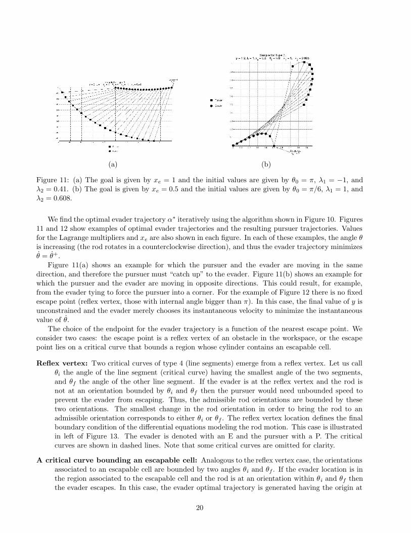
Figure 11: (a) The goal is given by xe = 1 and the initial values are given by θ0 = π, λ1 = −1, andλ2 = 0.41. (b) The goal is given by xe = 0.5 and the initial values are given by θ0 = π/6, λ1 = 1, andλ2 = 0.608.

We find the optimal evader trajectory α∗ iteratively using the algorithm shown in Figure 10. Figures11 and 12 show examples of optimal evader trajectories and the resulting pursuer trajectories. Valuesfor the Lagrange multipliers and xe are also shown in each figure. In each of these examples, the angle θis increasing (the rod rotates in a counterclockwise direction), and thus the evader trajectory minimizesθ = θ+.

Figure 11(a) shows an example for which the pursuer and the evader are moving in the samedirection, and therefore the pursuer must “catch up” to the evader. Figure 11(b) shows an example forwhich the pursuer and the evader are moving in opposite directions. This could result, for example,from the evader tying to force the pursuer into a corner. For the example of Figure 12 there is no fixedescape point (reflex vertex, those with internal angle bigger than π). In this case, the final value of y isunconstrained and the evader merely chooses its instantaneous velocity to minimize the instantaneousvalue of θ.

The choice of the endpoint for the evader trajectory is a function of the nearest escape point. Weconsider two cases: the escape point is a reflex vertex of an obstacle in the workspace, or the escapepoint lies on a critical curve that bounds a region whose cylinder contains an escapable cell.

Reflex vertex: Two critical curves of type 4 (line segments) emerge from a reflex vertex. Let us callθi the angle of the line segment (critical curve) having the smallest angle of the two segments,and θf the angle of the other line segment. If the evader is at the reflex vertex and the rod isnot at an orientation bounded by θi and θf then the pursuer would need unbounded speed toprevent the evader from escaping. Thus, the admissible rod orientations are bounded by thesetwo orientations. The smallest change in the rod orientation in order to bring the rod to anadmissible orientation corresponds to either θi or θf . The reflex vertex location defines the finalboundary condition of the differential equations modeling the rod motion. This case is illustratedin left of Figure 13. The evader is denoted with an E and the pursuer with a P. The criticalcurves are shown in dashed lines. Note that some critical curves are omitted for clarity.

A critical curve bounding an escapable cell: Analogous to the reflex vertex case, the orientationsassociated to an escapable cell are bounded by two angles θi and θf . If the evader location is inthe region associated to the escapable cell and the rod is at an orientation within θi and θf thenthe evader escapes. In this case, the evader optimal trajectory is generated having the origin at

20

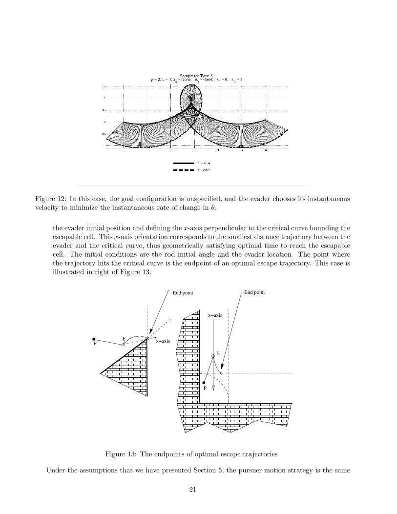
Figure 12: In this case, the goal configuration is unspecified, and the evader chooses its instantaneousvelocity to minimize the instantaneous rate of change in θ.

the evader initial position and defining the x-axis perpendicular to the critical curve bounding theescapable cell. This x-axis orientation corresponds to the smallest distance trajectory between theevader and the critical curve, thus geometrically satisfying optimal time to reach the escapablecell. The initial conditions are the rod initial angle and the evader location. The point wherethe trajectory hits the critical curve is the endpoint of an optimal escape trajectory. This case isillustrated in right of Figure 13.

��

��

��

��

x−axis

EP

E

P

End point

x

End point

x−axisx

Figure 13: The endpoints of optimal escape trajectories

Under the assumptions that we have presented Section 5, the pursuer motion strategy is the same

21

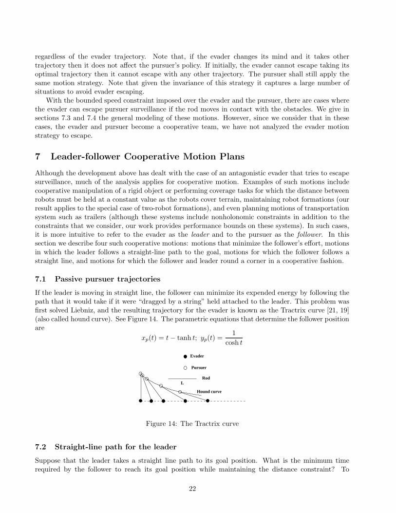
regardless of the evader trajectory. Note that, if the evader changes its mind and it takes othertrajectory then it does not affect the pursuer’s policy. If initially, the evader cannot escape taking itsoptimal trajectory then it cannot escape with any other trajectory. The pursuer shall still apply thesame motion strategy. Note that given the invariance of this strategy it captures a large number ofsituations to avoid evader escaping.

With the bounded speed constraint imposed over the evader and the pursuer, there are cases wherethe evader can escape pursuer surveillance if the rod moves in contact with the obstacles. We give insections 7.3 and 7.4 the general modeling of these motions. However, since we consider that in thesecases, the evader and pursuer become a cooperative team, we have not analyzed the evader motionstrategy to escape.

7 Leader-follower Cooperative Motion Plans

Although the development above has dealt with the case of an antagonistic evader that tries to escapesurveillance, much of the analysis applies for cooperative motion. Examples of such motions includecooperative manipulation of a rigid object or performing coverage tasks for which the distance betweenrobots must be held at a constant value as the robots cover terrain, maintaining robot formations (ourresult applies to the special case of two-robot formations), and even planning motions of transportationsystem such as trailers (although these systems include nonholonomic constraints in addition to theconstraints that we consider, our work provides performance bounds on these systems). In such cases,it is more intuitive to refer to the evader as the leader and to the pursuer as the follower. In thissection we describe four such cooperative motions: motions that minimize the follower’s effort, motionsin which the leader follows a straight-line path to the goal, motions for which the follower follows astraight line, and motions for which the follower and leader round a corner in a cooperative fashion.

7.1 Passive pursuer trajectories

If the leader is moving in straight line, the follower can minimize its expended energy by following thepath that it would take if it were “dragged by a string” held attached to the leader. This problem wasfirst solved Liebniz, and the resulting trajectory for the evader is known as the Tractrix curve [21, 19](also called hound curve). See Figure 14. The parametric equations that determine the follower positionare

xp(t) = t− tanh t; yp(t) =1

cosh t

Hound curve

Rod

Evader

Pursuer

L

Figure 14: The Tractrix curve

7.2 Straight-line path for the leader

Suppose that the leader takes a straight line path to its goal position. What is the minimum timerequired by the follower to reach its goal position while maintaining the distance constraint? To

22

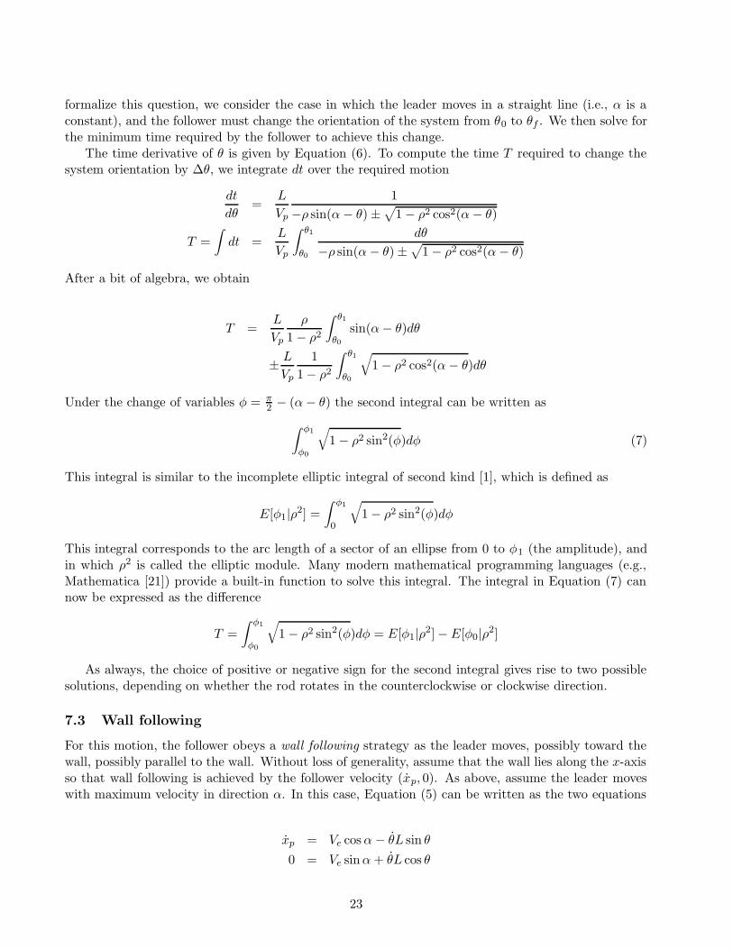
formalize this question, we consider the case in which the leader moves in a straight line (i.e., α is aconstant), and the follower must change the orientation of the system from θ0 to θf . We then solve forthe minimum time required by the follower to achieve this change.

The time derivative of θ is given by Equation (6). To compute the time T required to change thesystem orientation by ∆θ, we integrate dt over the required motion

dt

dθ=

L

Vp

1


1− ρ2 cos2(α− θ)

T =

∫

dt =L

Vp

∫ θ1

θ0

dθ


1− ρ2 cos2(α− θ)

After a bit of algebra, we obtain

T =L

Vp

ρ

1− ρ2

∫ θ1

θ0

sin(α− θ)dθ

±L

Vp

1

1− ρ2

∫ θ1

θ0

√

1− ρ2 cos2(α− θ)dθ

Under the change of variables φ = π2 − (α− θ) the second integral can be written as

∫ φ1

φ0

√

1− ρ2 sin2(φ)dφ (7)

This integral is similar to the incomplete elliptic integral of second kind [1], which is defined as

E[φ1|ρ2] =

∫ φ1

0

√

1− ρ2 sin2(φ)dφ

This integral corresponds to the arc length of a sector of an ellipse from 0 to φ1 (the amplitude), andin which ρ2 is called the elliptic module. Many modern mathematical programming languages (e.g.,Mathematica [21]) provide a built-in function to solve this integral. The integral in Equation (7) cannow be expressed as the difference

T =

∫ φ1

φ0

√

1− ρ2 sin2(φ)dφ = E[φ1|ρ2]−E[φ0|ρ

2]

As always, the choice of positive or negative sign for the second integral gives rise to two possiblesolutions, depending on whether the rod rotates in the counterclockwise or clockwise direction.

7.3 Wall following

For this motion, the follower obeys a wall following strategy as the leader moves, possibly toward thewall, possibly parallel to the wall. Without loss of generality, assume that the wall lies along the x-axisso that wall following is achieved by the follower velocity (xp, 0). As above, assume the leader moveswith maximum velocity in direction α. In this case, Equation (5) can be written as the two equations

xp = Ve cos α− θL sin θ

0 = Ve sinα + θL cos θ

23

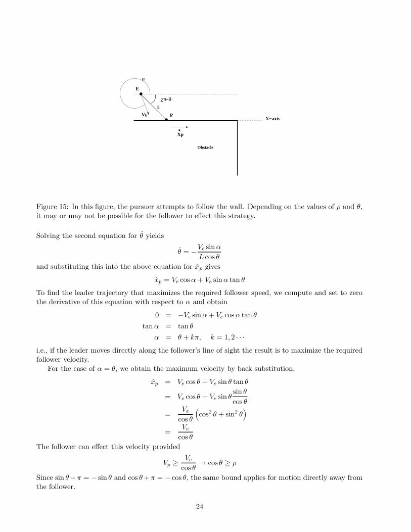
Obstacle

2π−θ

α

X−axis

Xp

L

V

E

PE

Figure 15: In this figure, the pursuer attempts to follow the wall. Depending on the values of ρ and θ,it may or may not be possible for the follower to effect this strategy.

Solving the second equation for θ yields

θ = −Ve sinα

L cos θ

and substituting this into the above equation for xp gives

xp = Ve cos α + Ve sinα tan θ

To find the leader trajectory that maximizes the required follower speed, we compute and set to zerothe derivative of this equation with respect to α and obtain

0 = −Ve sinα + Ve cos α tan θ

tan α = tan θ

α = θ + kπ, k = 1, 2 · · ·

i.e., if the leader moves directly along the follower’s line of sight the result is to maximize the requiredfollower velocity.

For the case of α = θ, we obtain the maximum velocity by back substitution,

xp = Ve cos θ + Ve sin θ tan θ

= Ve cos θ + Ve sin θsin θ

cos θ

=Ve

cos θ

(

cos2 θ + sin2 θ)

=Ve

cos θ

The follower can effect this velocity provided

Vp ≥Ve

cos θ→ cos θ ≥ ρ

Since sin θ +π = − sin θ and cos θ +π = − cos θ, the same bound applies for motion directly away fromthe follower.

24

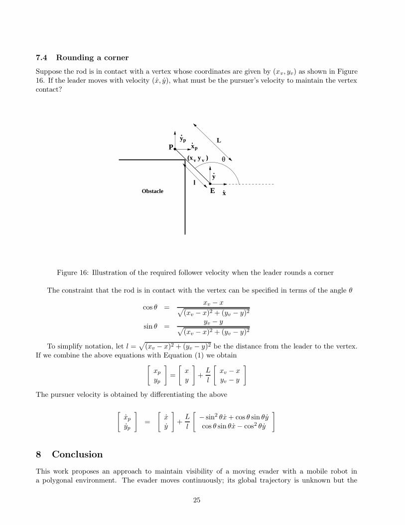
7.4 Rounding a corner

Suppose the rod is in contact with a vertex whose coordinates are given by (xv, yv) as shown in Figure16. If the leader moves with velocity (x, y), what must be the pursuer’s velocity to maintain the vertexcontact?

lObstacle

(xv y v )

y

x

pxp

y

θ

L

E

P

Figure 16: Illustration of the required follower velocity when the leader rounds a corner

The constraint that the rod is in contact with the vertex can be specified in terms of the angle θ

cos θ =xv − x

√

(xv − x)2 + (yv − y)2

sin θ =yv − y

√

(xv − x)2 + (yv − y)2

To simplify notation, let l =√

(xv − x)2 + (yv − y)2 be the distance from the leader to the vertex.If we combine the above equations with Equation (1) we obtain

[

xp

yp

]

=

[

xy

]

+L

l

[

xv − xyv − y

]

The pursuer velocity is obtained by differentiating the above

[

xp

yp

]

=

[

xy

]

+L

l

[

− sin2 θx + cos θ sin θycos θ sin θx− cos2 θy

]

8 Conclusion

This work proposes an approach to maintain visibility of a moving evader with a mobile robot ina polygonal environment. The evader moves continuously; its global trajectory is unknown but the

25

distribution of obstacles in the workspace is known in advance. We give necessary conditions for theexistence of a surveillance strategy.

The work presented in [5] gives an efficient algorithm to compute an optimal motion strategy totrack an evader. The method of [5] assumes a predictable evader. Our work relaxes this constraint.Our approach is able to track the evader even if the global trajectories of both evader and pursuer areunknown in advance, since it is possible to deduce the optimal motion policies of both pursuer andevader. In [5], the authors proposed as an improvement to their work to include a range constraint.Our paper presents that extension.

In game theoretic terms, we have solved the game of degree [13, 3] of maintaining visibility at afixed distance of a moving evader with a mobile robot in the presence of obstacles, for a single set ofescapable configurations.

The decision problem, which equivalent to answering the question Can the evader escape? dependson the optimal evader and pursuer motion policies. If the pursuer is able to track an evader that travelsthe optimal path then it will be able to track an evader that travels any other path.

Our analysis including bounded speeds holds for a single set of escapable configurations. If morethan one set is considered then a combinatorial problem arises. This combinatorial problem correspondsto define the optimal ordering to visit the escapable configurations. In this paper, we did not deal withthis combinatorial problem. We leave this latter problem for future work. However, note that oursufficiency condition for escaping without the bounded speed constraint includes any ordering to visitescapable configuration sets.

In [24], we have proposed a method able to determine the existence a solution, if there is delaybetween the evader and pursuer motion. In that work, we have assumed that the pursuer speed isunbounded. As future work, we would like to find a solution for the case of both delay and boundedpursuer speed. Finally, we want to consider dynamic and nonholonomic constraints.

Acknowledgment

The authors would like to thank Stephen Kloder and Jean Paul Laumond for helpful discussions.

References

[1] U.S. National Bureau of Standards, Handbook of Mathematical Functions with Formulas, Graphs,and Mathematical Tables. Edited by M Abramowitz and I.A. Stegun, 1964.

[2] J. Banon, Implementation and Extension of the Ladder Algorithm Proc. IEEE Int. Conf. onRobotics and Automation, Cincinnati Ohio, USA, pp. 1548-1553, 1990.

[3] T. Basar and G. Olsder, Dynamic Non cooperative Game Theory. Academic Press. 1982.

[4] C. Becker, H. Gonzlez-Banos, J.-C. Latombe and C. Tomasi, An intelligent observer. In LectureNotes in Control and Information Sciences 223, O. Khatib and J.K. Salisbury (eds.), Springer, NewYork, NY, pp. 153-160, 1997

[5] A. Efrat, H. H. Gonzalez-Banos, S. G. Kobourov, and L. Palaniappan. Optimal Motion Strategiesto Track and Capture a Predictable Target. Proc. IEEE Int. Conf. on Robotics and Automation,Taipei, Taiwan, pp. 411-423, 2003.

[6] B. Espiau, F. Chaumette, and P. Rives, A new approach to visual servoing in robotics. IEEE Trans.Robotics and Automation., 8(3):313-326, June 1992.

26

[7] P. Fabiani and J.-C. Latombe, Tracking a partially predictable object with uncertainty and visibilityconstraints: a game-theoretic approach, Proc. Int. Joint Conf. on Artificial Intelligence, Stockholm,Sweden, pp. 942-947, 1999.

[8] L. Guibas, J.-C. Latombe,S.M. LaValle, D. Lin, R. Motwani, Visibility-based pursuit-evasion in apolygonal environment, Proc. 5th Int. Workshop on Algorithms and Data Structures (WADS’97),Halifax, Nova Scotia, Canada; published as Lecture Notes in Computer Science 1272, F. Dehne, A.Rau-Chaplin, J.R. Sack, and R. Tamassia (eds.), pp. 17-30, 1997.

[9] O. Hajek. Pursuit Games. Academic Press, New York, 1965.

[10] J. Hespanha, M. Prandini, and S. Sastry, Probabilistic Pursuit-Evasion Games: A one-step Nashapproach, Proc. IEEE Conference on Decision and Control, Sydney, Australia, pp. 2272-2277, 2000.

[11] H.H. Gonzalez, C.-Y. Lee and J.-C. Latombe, Real-Time Combinatorial Tracking of a TargetMoving Unpredictably Among Obstacles, Proc. IEEE Int. Conf. on Robotics and Automation,Arlington VA, USA, pp. 1683-1690, 2002.

[12] S.Hutchinson, G. Hager and P. Corke. A tutorial on visual servo control. In IEEE Trans. Roboticsand Automation, Vol 12 No.5, pp. 651-670, Oct 1996.

[13] R. Isaacs. Differential Games: A Mathematical Theory with Applications to Warfare and Pursuit,Control and Optimization . Wiley, New York,NY, 1975.

[14] V. Isler, S. Kannan, and S. Khanna, Locating and Capturing an Evader in a Polygonal Environ-ment. In Sixth International Workshop on the Algorithmic Foundations of Robotics, Utrecht/Zeist,The Netherlands, pp. 351-367, 2004.

[15] V. Isler, S. Kannan, and S. Khanna, Randomized Pursuit-Evasion in a Polygonal Environment.IEEE Trans on Robotics, 5(21):875-884, Oct 2005.

[16] B. Jung and G. Sukhatme, Tracking targets using multiple robots: the effect of environmentocclusion, Journal Autonomous Robots, vol. 13, No 3 pp. 191-205, November 2002.

[17] S.M. LaValle, H.H. Gonzalez-Banos, C. Becker and J.-C. Latombe, Motion Strategies for Maintain-ing Visibility of a Moving Target In Proc IEEE Int. Conf. on Robotics and Automation, AlbuquerqueNew Mexico, USA, pp.737-742, 1997.

[18] S.M. LaValle, J. Hinrichsen, Visibility-based pursuit-evasion: An extension to curved environ-ments, In Proc IEEE Int. Conf. on Robotics and Automation, Detroit Michigan, USA, pp. 1677-1682, 1999.

[19] J.D. Lawrence, A Catalog of Special Plane Curves. Dover Pub., 1971.

[20] J.-C. Latombe, Robot Motion Planning. Kluwer Academic Publishers, 1991.

[21] http://mathworld.woldfram.com/ EllipticIntegraloftheSecondKind.html

[22] R. Murrieta-Cid, H.H. Gonzalez-Banos and B. Tovar, A Reactive Motion Planner to MaintainVisibility of Unpredictable Targets Proc. IEEE Int. Conf. on Robotics and Automation, ArlingtonVA, USA, pp. 4242-4248, 2002.

27

[23] R. Murrieta-Cid, A. Sarmiento and S. Hutchinson, A Motion Planning Strategy to MaintainVisibility of a Moving Target at a Fixed Distance in a Polygon Proc. Int. Conf. on AdvancedRobotics, Coimbra Portugal, pp. 228-233, 2003.

[24] R. Murrieta-Cid, A. Sarmiento and S. Hutchinson, On the Existence of a Strategy to Maintaina Moving Target within the Sensing Range of an Observer Reacting with Delay Proc. IEEE Int.Conf. on Intelligent Robots and Systems, Las Vegas Nevada, USA, pp. 1184-1191, 2003.

[25] R. Murrieta-Cid, A. Sarmiento, S. Bhattacharya and S. Hutchinson, Maintaining Visibility of aMoving Target at a Fixed Distance: The Case of Observer Bounded Speed Proc. IEEE Int. Conf.on Robotics and Automation, New Orleans Louisiana, USA, pp. 479-484, 2004.

[26] T. Muppirala, R. Murrieta-Cid, and S. Hutchinson. Optimal motion strategies based on criticalevents to maintain visibility of a moving target. Proc IEEE Int. Conf. on Robotics and Automation,Barcelona, Spain, pp. 3837-3842, 2005.

[27] L. Parker Algorithms for Multi-Robot Observation of Multiple Targets, Journal AutonomousRobots, vol. 12, No 3, pp. 231-255, May 2002.

[28] T.D. Parsons Pursuit-evasion in a graph. In Y. Alani and D.R. Lick, editors, Theory and Appli-cation of Graphs, pages 426-441, Springer-Verlag, Berlin, 1976.

[29] S. Petitjean, D. Kriegman and J. Ponce, Computing exact aspect graphs of curved objects: alge-braic surfaces. Int Journal on Computer Vision, 9:231-255, Dec 1992.

[30] S. Shas, S. Rajko and S.M. LaValle, Visibility-based pursuit-evasion in an unknown planar envi-ronment International Journal on Robotics Research, 23(1):3-26, January 2004.

[31] J.T. Schwartz and M. Sharir, On the Piano Movers’ Problem: I. The Case of a Two-DimensionalRigid Polygon Body Moving Amidst Polygonal Barriers, Communications on Pure and AppliedMathematics, vol 36, 345-398, 1987.

[32] I. Suzuki and M. Yamashita Searching for a mobile intruder in a polygonal region. SIAM Journalon Computing, 21(5):863-888, October 1992.

[33] R. Vidal, O. Shakernia, H.Jin, D. Hyunchul and S. Sastry, Probabilistic Pursuit-Evasion Games:Theory, Implementation, and Experimental Evaluation, IEEE Trans. Robotics and Automation,18(5):662-669, October, 2002.

28

Surveillance Strategies for a Pursuer with Finite Sensor Range

Documents