SurfConv: Bridging 3D and 2D Convolution for RGBD Images Hang Chu 1,2 Wei-Chiu Ma 3 Kaustav Kundu 1,2 Raquel Urtasun 1,2,3 Sanja Fidler 1,2 1 University of Toronto 2 Vector Institute 3 Uber ATG {chuhang1122, kkundu, fidler}@cs.toronto.edu {weichiu, urtasun}@uber.com Abstract The last few years have seen approaches trying to com- bine the increasing popularity of depth sensors and the suc- cess of the convolutional neural networks. Using depth as additional channel alongside the RGB input has the scale variance problem present in image convolution based ap- proaches. On the other hand, 3D convolution wastes a large amount of memory on mostly unoccupied 3D space, which consists of only the surface visible to the sensor. Instead, we propose SurfConv, which “slides” compact 2D filters along the visible 3D surface. SurfConv is formulated as a simple depth-aware multi-scale 2D convolution, through a new Data-Driven Depth Discretization (D 4 ) scheme. We demonstrate the effectiveness of our method on indoor and outdoor 3D semantic segmentation datasets. Our method achieves state-of-the-art performance while using less than 30% parameters used by the 3D convolution based ap- proaches. 1. Introduction While 3D sensors have been popular in the robotics community, they have gained prominence in the computer vision community in the recent years. This has been the effect of extensive interest in applications such as au- tonomous driving [11], augmented reality [32] and urban planning [47]. These 3D sensors come in various forms such as active LIDAR sensors, structured light sensors, stereo cameras, time-of-flight cameras, etc. These range sensors produce a 2D depth image, where the value at every pixel location corresponds to the distance traveled by a ray from the sensor through the pixel location, before it hits a visible surface in the 3D scene. Recent success of convolutional neural networks for RGB input images [24] have raised interests in using them for depth data. One of the common approaches is to use handcrafted representations of the depth data and treat them as additional channels alongside the RGB input [13, 9]. Code&data: https://github.com/chuhang/SurfConv Image Convolution 3D Convolution Surface Convolution Figure 1. A 3D sensor captures a surface at a single time frame. 2D im- age convolution does not utilize 3D information and suffers from scale variance. 3D convolution solves scale variance, but suffers from non- volumetric surface input where majority of voxels are empty. We propose surface convolution, that convolutes 2D filters along the 3D surface. While this line of work has shown that additional depth in- put can improve performance on several tasks, it is not able to solve the scale variance problem of 2D convolutions. In the top of Fig. 1, we can see that for two cars at different distances, the receptive fields of a point have the same size. This means that models are required to learn to recognize 3002

Welcome message from author
This document is posted to help you gain knowledge. Please leave a comment to let me know what you think about it! Share it to your friends and learn new things together.
Transcript

SurfConv: Bridging 3D and 2D Convolution for RGBD Images
Hang Chu1,2 Wei-Chiu Ma3 Kaustav Kundu1,2 Raquel Urtasun1,2,3 Sanja Fidler1,2
1University of Toronto 2Vector Institute 3Uber ATG
{chuhang1122, kkundu, fidler}@cs.toronto.edu {weichiu, urtasun}@uber.com
Abstract
The last few years have seen approaches trying to com-
bine the increasing popularity of depth sensors and the suc-
cess of the convolutional neural networks. Using depth as
additional channel alongside the RGB input has the scale
variance problem present in image convolution based ap-
proaches. On the other hand, 3D convolution wastes a large
amount of memory on mostly unoccupied 3D space, which
consists of only the surface visible to the sensor. Instead,
we propose SurfConv, which “slides” compact 2D filters
along the visible 3D surface. SurfConv is formulated as
a simple depth-aware multi-scale 2D convolution, through
a new Data-Driven Depth Discretization (D4) scheme. We
demonstrate the effectiveness of our method on indoor and
outdoor 3D semantic segmentation datasets. Our method
achieves state-of-the-art performance while using less than
30% parameters used by the 3D convolution based ap-
proaches.
1. Introduction
While 3D sensors have been popular in the robotics
community, they have gained prominence in the computer
vision community in the recent years. This has been
the effect of extensive interest in applications such as au-
tonomous driving [11], augmented reality [32] and urban
planning [47]. These 3D sensors come in various forms
such as active LIDAR sensors, structured light sensors,
stereo cameras, time-of-flight cameras, etc. These range
sensors produce a 2D depth image, where the value at every
pixel location corresponds to the distance traveled by a ray
from the sensor through the pixel location, before it hits a
visible surface in the 3D scene.
Recent success of convolutional neural networks for
RGB input images [24] have raised interests in using them
for depth data. One of the common approaches is to use
handcrafted representations of the depth data and treat them
as additional channels alongside the RGB input [13, 9].
Code&data: https://github.com/chuhang/SurfConv
Image Convolution
3D Convolution
Surface Convolution
Figure 1. A 3D sensor captures a surface at a single time frame. 2D im-
age convolution does not utilize 3D information and suffers from scale
variance. 3D convolution solves scale variance, but suffers from non-
volumetric surface input where majority of voxels are empty. We propose
surface convolution, that convolutes 2D filters along the 3D surface.
While this line of work has shown that additional depth in-
put can improve performance on several tasks, it is not able
to solve the scale variance problem of 2D convolutions. In
the top of Fig. 1, we can see that for two cars at different
distances, the receptive fields of a point have the same size.
This means that models are required to learn to recognize
13002

the same object in different inputs.
To overcome this issue, an alternative is to represent the
data as a 3D grid and use 3D convolution on it [49]. For
such a dense representation, it requires huge computation
and memory resources. This limits the resolution in all three
dimensions. Furthermore, since 3D sensor captures the in-
formation of how far the objects are from the sensor at a
single frame, the visible surface of the scene occludes the
rest of the 3D volume. Thus, the information in the input
occupies an extremely small fraction (∼ 0.35%1) of the en-
tire volume. This results in the 3D convolution based ap-
proaches to spend a large fraction of time and memory on
the unoccupied empty space shown in the middle of Fig. 1.
We propose to reformulate the default 3D convolution as
Surface Convolution (SurfConv) for a single frame RGBD
input. Instead of “sliding” 3D filters in the voxel space,
we slide compact 2D filters along the observed 3D sur-
face. This helps us to exploit the surface nature of our
input and help the network learn scale-invariant represen-
tations (bottom of Fig. 1). A straight-forward implemen-
tation of surface convolutions is challenging since it re-
quires depth-dependent rescaling at every location, which
is a computational bottleneck. To address this problem, we
propose a Data-Driven Depth Discretization (D4) scheme,
which makes surface convolution practically feasible. We
use our approach to show state-of-the-art results on the
single-view 3D semantic segmentation task in KITTI [11]
and NYUv2 [40] benchmarks. To summarize, our main
contributions are:
• We propose Surface Convolution, that processes single
frame 3D data in accordance with its surface nature.
• We propose to realize Surface Convolution through a
Data-Driven Depth Discretization scheme, which of-
fers a simple yet effective solution that achieves state-
of-the-art single view 3D semantic segmentation.
2. Related Work
Deep 2D RGBD Representations. In the last few years,
2D CNNs have been used to create powerful feature de-
scriptors for images [24], and can learn complex patterns in
the data [57]. One of the approaches to extend the success
of these 2D convolutions to range data, is by projecting the
3D data into multiple viewpoints, each of which is treated
as a 2D input [4, 34, 39, 44]. However, the computation
time scales linearly with the number of views. Since a sin-
gle frame RGBD image sees only the unoccluded portion
of the 3D world, the visible surfaces from drastically differ-
ent viewpoints might not align with that of the input cam-
era viewpoint. Furthermore, reasoning about multiple view-
1Calculated with the standard 0.1m resolution for [11] and 0.02m res-
olution for [40]
points does not lead to a natural, interpretable 3D descrip-
tion of the scene into parts and their spatial relations [17].
Another alternative is to simply use handcrafted depth
representations and treat them as additional channels along-
side the RGB input. Such approaches have shown to im-
prove for tasks such as 3D shape retrieval [9, 50], seman-
tic segmentation [12, 13, 26, 29] and 3D object detec-
tion [3, 7, 8, 25].
3D Convolution. To handle the scale variance, 3D con-
volution learns the correlations directly in the 3D space. To
represent the point cloud information, input representations
such as occupancy grids [20, 31, 38] and TSDF [5, 10, 42,
53, 55] have been explored.
One of the key challenges in 3D convolution is the fact
that increasing the input dimensions by one can lead to sig-
nificant increase the memory budget. Thus, common prac-
tices are to either limit the input resolution to a low res-
olution grid, or have a higher resolution but with reduced
network parameters [43]. Since the range data is sparse in
nature, approaches such as [8, 37, 46] have also exploited it
to reduce the memory consumption of the activation maps.
However, these efforts are difficult to implement and are
nontrivial to scale to a wide variety of tasks in challenging
benchmarks.
Another disadvantage of using voxel grids is that it as-
sumes that the scene has an Euclidean structure and is not
invariant to transformations such as isotropy and non-rigid
deformations. This limitation is overcome by considering
the points as members of an orderless set, which are used
along a global representation [33, 35, 52] of the 3D volume.
Approaches such as [23, 45] have used a CRF for post-
processing the semantic segmentation prediction from a 3D
ConvNet. [36] used a 3D graph neural network to iteratively
improve the unary semantic segmentation predictions. Our
approach can be used to provide better a unary term for
these methods.
3D Surface based Descriptors. Convoluting in the volu-
metric space, a different approach would be to reason along
the surface of the 3D volumes. [21] introduced the idea of
spin images, which builds a 3D surface based descriptors
for object recognition. [19] learns a generative model to
produce object structure through surface geometry. [30, 1]
extended the idea of convolutions to non-Euclidean struc-
tures by learning anisotropic heat kernels which relates to
surface deformity. However, such methods require point
associations to learn the filters, which are difficult to obtain
for range data depicting natural scenes. [22] combines the
segmentation results of multiple views into a surface rep-
resentation of the 3D object. This is followed by a post-
processing step with a CRF which smoothens the labels
along the surface geometry. Such smoothening CRF can
3003

be used to further improve the results of our approach as
well.
Multi-Scale 2D Convolutions. To get better perfor-
mance, a host of approaches have used multi-scale input
to for tasks such as semantic segmentation [2, 27], optical
flow [48], and detection [15, 18]. Other approaches include
adaptively learning pixel-wise scale [6, 54], and upscaling
feature activations to combine multiple scales for the final
prediction [28, 56]. The key difference of such approaches
with ours is that these scales are arbitrary and do not utilize
the 3D geometry of the scene.
3. Method
An image from a single frame RGBD camera captures
only the visible surface of the 3D space. Instead of wasting
memory on the entire 3D volume, we introduce SurfConv,
which concentrates the computation only along the visible
surface. In Sec. 3.1 we derive SurfConv, which approx-
imates 3D convolution operation to a depth-aware multi-
scale 2D convolution. We justify the approximation as-
sumption and its implications in Sec. 3.2. In Sec. 3.3, we
describe the D4 scheme that determines the scales in a sys-
tematic fashion.
3.1. Surface Convolution
Notation. We denote a point detected by the sensor as p.
Three scalars (px,py,pz) represents its position in 3D. Fol-
lowing the classic camera model, we set the sensor position
(aperture) at the origin, and the principal axis as the posi-
tive z direction. We define an image plane, and the distance
from the image plane to the camera aperture is defined as
the focal length. For simplicity, we rescale the coordinates
such that focal length is equal to 1. We can then compute
the image plane coordinates of point p as
pi =px
pz
, pj =py
pz(1)
We denote the information (e.g. color intensity values)
of point p as Ip, and its semantic class label as Lp. At high
level, semantic segmentation can be formulated as
Lp = F(Ip′∈R(p)) (2)
where F is a function of choice (e.g. a convolutional neural
network), and R(p) defines a local neighborhood of point
p. We refer to R(p) as the receptive field at point p, as
commonly used in literatures. Different types of convolu-
tion take different forms of F and R. Next, we mainly focus
on the receptive field R, as it defines the local neighborhood
that affects the final segmentation decision.
Image Convolution. In image convolution, the receptive
field of point p is defined as Rimg(p) = {p′}, such that
Figure 2. A 2D illustration of our local planarity assumption. Gray curve
shows the visible surface, solid green line shows the approximation plane,
for the center point’s local neighborhood.
pi′ ∈ [pi −∆img,pi +∆img]
pj′ ∈ [pj −∆img,pj +∆img]
(3)
where ∆img defines the receptive field radius. We can see
that Rimg(p) defines a rectangle on the projected image
plane. The receptive field has the same number of pixels
regardless of the center point’s distance. Therefore, image
convolution suffers from the scale variance problem.
3D Convolution. To utilize the 3D information, espe-
cially in the depth dimension, 3D convolution has been in-
troduced. In 3D convolution, the receptive field can be de-
fined by trivially extending into all three spatial dimensions,
i.e. R3d(p) = {p′} such that
px′ ∈ [px −∆3d,px +∆3d]
py′ ∈ [py −∆3d,py +∆3d]
pz′ ∈ [pz −∆3d,pz +∆3d]
(4)
This defines a 3D cuboid centered at point p, with radius
∆3d. In 3D convolution, the receptive field becomes inde-
pendent to depth and no longer suffers from scale variance.
However, for a single-frame 3D sensor, the actual 3D data is
essentially a surface back-projected from the image plane.
This means at any given 3D cubic receptive field, the major-
ity of space is empty, which makes training F difficult. To
address the sparsity problem, approaches have used Trun-
cated Signed Distance Function (TSDF) [55] and flipped-
TSDF [43] that fills the empty space, or decrease the voxel
resolution [8].
Local Planarity Assumption. We seek a solution that
directly operates along the visible surface, where the mean-
ingful information resides. To achieve this, we first intro-
duce the local planarity assumption. Then we show that
under this assumption, we can reformulate 3D convolution
as a depth-aware multi-scale 2D convolution. We name this
reformulated approximation as Surface Convolution (Surf-
Conv).
The local planarity assumption is defined as: All neigh-
bor points are approximated to have the same depth as the
receptive field center. Fig. 2 illustrates the approximation
assumption. Under this assumption, we have
pz′ = pz, ∀p′ ∈ R3d(p) (5)
3004

Surface Convolution. Under the local planarity as-
sumption, we can transform the 3D convolution receptive
field into the SurfConv receptive field. Combining Eq. 1
and Eq. 4, we get
pi′pz
′ = px′ ∈ [px −∆3d,px +∆3d] (6)
Then we apply the local planarity assumption as in Eq. 7,
and get
pi′ ∈ [
px −∆3d
pz
,px +∆3d
pz
] (7)
We can further apply the projection matrix, and obtain the
final receptive field definition of SurfConv: Rsf (p) = {p′}such that
pi′ ∈ [pi −
∆sf
pz
,pi +∆sf
pz
]
pj′ ∈ [pj −
∆sf
pz
,pj +∆sf
pz
]
(8)
where ∆sf = ∆3d defines the receptive field radius in the
3D space. In this way, the SurfConv receptive field de-
fines a square image region, whose size is controlled by the
center point’s depth. This means SurfConv is essentially
a depth aware multi-scale 2D convolution. This bridges
the 3D and 2D perspectives, and avoids the disadvantages
of either method. Compared to 2D convolution, SurfConv
utilizes 3D data and does not suffer from scale variance.
Compared to 3D convolution, SurfConv not only saves the
preprocessing step of filling empty voxels, but also enables
learning compact, parameter-efficient convolution 2D filters
that directly targets the real-world scale of the input data.
In SurfConv, pz ∈ R is a continous variable. This means
for each point, we need to dynamically resize the receptive
field based on its size determined by Eq. 9, before passing
it to the recognition module F that takes fixed size input.
This is computationally inefficient in practice. To address
this problem, we further replace the continues depth with a
set of discretized values, i.e. pz ∈ {z1, z2, ...zN }. We refer
to N as the level of SurfConv. With the discretized depth,
we can cache N levels of the image pyramid. Note that
since we are interested in surface convolution, each pixel in
the original RGBD image belongs to exactly one level of the
pyramid. Fig. 3 shows a toy example of our discretization
process.
3.2. Bridging 3D and 2D Convolution
In SurfConv, we discretize the z dimension into N lev-
els and maintain the full resolution in x and y dimensions.
Thus, our surface convolution can be seen as a deformed
version of general 3D convolution, where SurfConv has
coarser z resolution consisting of N levels, and divides the
original camera
SurfConv at z1
SurfConv at z2
Figure 3. A toy example of discretized SurfConv. In each row, left side
shows the scene and projection plane in cyan, right side shows the image.
Green bars show boundaries separating discretization levels. At each Sur-
fConv level, only points that have depth within the level are visible. The
blue and red objects remain equal-sized to SurfConv, despite their different
depth.
3D space into a z-stretched voxel grid. The memory con-
straints of current day GPUs limits the resolution of the in-
put. In 3D convolution, the 3D space is discretized simi-
larly in all three axes. This results in large grids and low-
ered maximum feasible resolution. In contrast, SurfConv
maintains the full resolution along axes parallel to the im-
age projection plane (x and y), and have a much coarser
resolution for the axis perpendicular to the image plane (i.e.
z). In an RGBD image, the information only resides along
the visible surface. This motivates the lower z resolution,
because information is scarce along this direction. Practi-
cally, SurfConv can be simply implemented with a depth-
aware multi-scale 2D convolution. Each depth level con-
sists a proportionally scaled version of the input, masked to
contain points within its depth range. Standard 2D CNN
training is applied to all levels simultaneously. Therefore,
SurfConv can easily benefit from networks pre-trained on a
variety of large-scale 2D image datasets.
3.3. D4: DataDriven Depth Discretization
To obtain a set of discretized depth levels, uniform bins
are sub-optimal. This is because in single-viewpoint input
3005

Figure 4. Point depth distribution at different environment. The distribu-
tion leans heavily to the lower side due to occlusion and sensor resolution.
Statistics obtained from NYUv2 [40] and KITTI [11].
data, near points significantly out-number far points due
to occlusion and decreasing resolution over depth. Fig. 4
shows actual depth distributions from real indoor and out-
door data. Therefore, uniform bins result in unbalanced data
allocation between levels, i.e. the first few levels have al-
most all points, while the last few levels are almost empty.
To address this problem, we introduce the D4 scheme.
Instead of dividing levels evenly, we compute level bound-
aries such that all levels contribute the same amount of in-
fluence to the segmentation model F. First, we define the
importance function of a point as
Θ(p) = pzγ (9)
where we refer to γ as the importance index. We use the
importance function to assign a weight to each input point,
then we find N discretization levels such that all levels pos-
sess the same amounts summed importance.
Intuitively, with γ = 0, all points are equally important
regardless of their depth. As result, all levels are allocated
with same number of image pixels. With γ = 2, a point’s
influence is proportional to the back-projected 3D surface
area it covers. As result, all levels have equal amount of
total 3D surface area after the discretization and allocation.
Ideally, γ = 2 seems the optimal setting because it
divides the visible surface area evenly to different lev-
els. However, we argue that γ should instead be a hyper-
parameter. Data quality decreases over distance for sensors,
i.e. the farther an object is, the less detailed measurement a
sensor receives. A farther object occupies a smaller field of
view from the sensor’s viewpoint. This means lower reso-
lution, hence lower capture quality. Additionally, in sensors
such as stereo cameras and Microsoft Kinect, precision de-
creases as depth increases, making farther points inherently
more noisy. Therefore, in order to learn the best recognition
model, there exists a tradeoff between trusting near clear
data, and paying attention to adapt to far noisy data. In other
words, the best index is determined by γ = 2 − ζ, where ζquantifies this near-far tradeoff. It is difficult to analytically
compute ζ, because it depends on the actual sensor configu-
ration and scene properties. Therefore, we tune ζ, hence γ,
through validation on the actual data.
4. Experimental Results
We demonstrate the effectiveness of our approach by
showing results on two real-world datasets (KITTI [11] and
NYUv2 [40]) for the 3D semantic segmentation task.
4.1. Experimental Setup
CNN model. We use the skip-connected fully convolu-
tional architecture [29] with two different backbones:
1. ResNet-18 [16]: We modify the size of all convolu-
tional kernels to 3 × 3 and experiment with different
number of feature channels in each layer. We try light
and heavy weight versions where the number of fea-
ture channels are 1/4, 1/2, same, or twice of the num-
ber of original channels. The input to our network is
a 6-channel RGB+HHA [13] image. This network has
been trained from scratch, similar to the baseline 3D
convolution based approaches.
2. VGG-16 [41]: We particularly choose this model be-
cause it is conventionally used in previous work on the
NYUv2 dataset [29, 14]. The input to this network is
the standard RGB image. This model has been pre-
trained on the Imagenet dataset.
Using the light weight models, we show that our per-
formance is competitive (NYUv2) or better (KITTI) than
the state-of-the-art 3D convolution based approaches even
with about a quarter of their parameters. Since the memory
requirement of our network is low compared to 3D convo-
lution based approaches, we can take advantage of heavier
models to further improve our performance. Moreover, our
approach can take advantage of pre-trained weights on ex-
isting large scale 2D datasets. For training our networks, we
follow FCN-8s and use the logarithm loss function.
Baselines. We compare our approach with Conv3D [45,
43], PointNet [33], and DeformCNN [6]. For Conv3D, we
use the SSCNet architechture [43], and train it with three
variations of gravity-aligned voxel input: RGB, flipped-
TSDF, and both. We follow [43] and use the maximum
possible voxel resolution that can fit a single-sample batch
into 12GB memory, which results in a 240×144×240 voxel
grid (with 2cm resolution) on NYUv2, and a 400×60×320
voxel grid (with 10cm resolution) on KITTI. The points that
fall into the same voxel are given the same predicted label
in inference.
For PointNet, we directly use the published source code,
and train it on three types of input: original point cloud,
gravity-algined point cloud, and RGB plus gravity align-
ment. We randomly sample points from the point cloud as
suggested in the paper. Specifically, we set the sample num-
ber as 25K, which fills 12GB memory with batch size 8.
For DeformCNN, we replace res5 layers with de-
formable convolution as recommended in [6]. We try jointly
3006
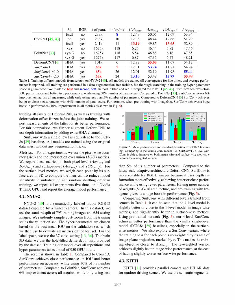
3d RGB # of para. infer./ms IOUimg Accimg IOUsurf Accsurf
Conv3D [45, 43]
ftsdf no 233k 8 12.43 50.05 12.69 53.34
no yes 238k 10 12.36 48.44 12.66 51.29
ftsdf yes 241k 11 13.19 49.85 13.65 52.89
PointNet [33]
xyz no 1675k 118 6.25 46.44 5.82 47.46
xyz-G no 1675k 118 6.54 46.88 6.16 47.85
xyz-G yes 1675k 117 6.87 47.35 6.47 48.21
DeformCNN [6] HHA yes 101k 6 12.82 55.05 11.67 54.12
SurfConv1 HHA yes 65k 5 12.31 53.74 11.27 54.24
SurfConv4-γ1.0 HHA yes 65k 26 12.01 52.19 11.98 55.44
SurfConv4-γ2.0 HHA yes 65k 24 13.10 53.48 12.79 55.99Table 1. Training different models from scratch on NYUv2 [40]. All models are trained till convergence for five times, and average perfor-
mance is reported. All training are performed in a data-augmentation-free fashion, but thorough searching in the training hyper-parameter
space is guaranteed. We mark the best and second best method in blue and red. Compared to Conv3D [45, 43], SurfConv achieves close
IOU performance and better Acc performance, while using 30% number of parameters. Compared to PointNet [33], SurfConv achieves 6%
improvement across all measures, while only using less than 5% number of parameters. Compared to DeformCNN [6] SurfConv achieves
better or close measurements with 64% number of parameters. Furthermore, when pre-training with ImageNet, SurfConv achieves a huge
boost in performance (10% improvement in all metrics as shown in Fig. 5).
training all layers of DeformCNN, as well as training with
deformation offset frozen before the joint training. We re-
port measurements of the latter for its better performance.
For fair comparison, we further augment DeformCNN to
use depth information by adding extra HHA channels.
SurfConv with a single level is equivalent to the FCN-
8s [29] baseline. All models are trained using the original
data as-is, without any augmentation tricks.
Metrics. For all experiments, we use the pixel-wise accu-
racy (Acc) and the intersection over union (IOU ) metrics.
We report these metrics on both pixel-level (Accimg and
IOUimg) and surface-level (Accsurf and IOUsurf ). For
the surface level metrics, we weigh each point by its sur-
face area in 3D to compute the metrics. To reduce model
sensitivity to initialization and random shuffling order in
training, we repeat all experiments five times on a Nvidia
TitianX GPU, and report the average model performance.
4.2. NYUv2
NYUv2 [40] is a semantically labeled indoor RGB-D
dataset captured by a Kinect camera. In this dataset, we
use the standard split of 795 training images and 654 testing
images. We randomly sample 20% rooms from the training
set as the validation set. The hyper-parameters are chosen
based on the best mean IOU on the validation set, which
we then use to evaluate all metrics on the test set. For the
label space, we use the 37-class setting [13, 36]. To obtain
3D data, we use the hole-filled dense depth map provided
by the dataset. Training our model over all repetitions and
hyper-parameters takes a total of 950 GPU hours.
The result is shown in Table 1. Compared to Conv3D,
SurfConv achieves close performance on IOU and better
performance on accuracy, while using 30% of its number
of parameters. Compared to PointNet, SurfConv achieves
6% improvement across all metrics, while only using less
Figure 5. Mean performance and standard deviation of NYUv2 finetun-
ing. Comparing to the vanilla CNN model (i.e. SurfConv1), 4-level Sur-
fConv is able to improve on both image-wise and surface-wise metrics. r
denotes the reweighted version.
than 5% of its number of parameters. Compared to the
latest scale-adaptive architecture DeformCNN, SurfConv is
more suitable for RGBD images because it uses depth in-
formation more effectively, achieving better or close perfor-
mance while using fewer parameters. Having more number
of weights (VGG-16 architecture) and pre-training with Im-
agenet gives us a huge boost in performance (Fig. 5).
Comparing SurfConv with different levels trained from
scratch in Table 1, it can be seen that the 4-level model is
slightly better or close to the 1-level model in image-wise
metrics, and significantly better in surface-wise metrics.
Using pre-trained network (Fig. 5), our 4-level SurfConv
achieves better performance than the vanilla single-level
model (FCN-8s [29] baseline), especially in the surface-
wise metrics. We also explore a SurfConv variant where
the training loss for each point is re-weighted by its area of
image-plane projection, marked by r. This makes the train-
ing objective closer to Accimg . The re-weighted version
achieves slightly better image-wise performance, at the cost
of having slightly worse surface-wise performance.
4.3. KITTI
KITTI [11] provides parallel camera and LIDAR data
for outdoor driving scenes. We use the semantic segmenta-
3007

NYUv2-37class KITTI-11classFigure 6. Average improved percentage of per-class surface IOU, using multi-level SurfConv over the single-level baseline, with the exact same CNN
model F (Eq. 2). Models are trained from scratch. On NYUv2, we improve 27/37 classes with 1.40% mean IOU increasement. On KITTI, we improve 8/11
classes with 4.31% mean IOU increasement.
NYUv2-37class KITTI-11classFigure 7. Same as Fig. 6, but finetuning from ImageNet instead of training from scratch. On NYUv2, multi-level SurfConv improves 26/37 classes with
0.99% mean IOU increasement, from the single-level baseline. On KITTI, multi-level SurfConv improves 11/11 classes with 9.86% mean IOU increasement.
tion annotation provided in [51], which contains 70 training
and 37 testing images from different scenes, with high qual-
ity pixel annotations in 11 categories. Due to the smaller
dataset size and lack of standard validation split, we di-
rectly validate all compared methods on the held-out test-
ing set. To obtain dense points from sparse LIDAR input,
we use a simple real-time surface completion method that
exhaustively join adjacent points into mesh triangles. The
densified points are used as input for all methods evaluated.
The smaller size of KITTI allows us to thoroughly explore
different settings of SurfConv levels, influence index γ, as
well as CNN model capacity. Our KITTI experiments take
a total of 750 GPU hours.
Baseline comparisons. Table 2 lists the comparison with
baseline methods. SurfConv outperforms all comparisons
in all metrics. In KITTI, the median maximum scene
depth is 75.87m. This scenario is particularly difficult for
Conv3D, because voxelizing the scene with sufficient res-
olution would result in large tensors and makes training
Conv3D difficult. On the contrary, SurfConv can be eas-
ily trained because its compact 2D filters do not suffer from
insufficient memory budget. DeformCNN performs better
than image convolution (i.e. SurfConv1) for its deforma-
tion layers that adapts to object scale variance. However,
multi-level SurfConv achieves more significant improve-
ment, demonstrating its capablity of using RGBD data more
effectively.
IOUimg Accimg IOUsurf AccsurfConv3D [45, 43] 17.53 64.54 17.38 62.58
PointNet [33] 9.41 55.06 9.07 64.38
DeformCNN [6] 34.24 79.17 27.51 73.36
SurfConv1 33.67 79.13 26.56 72.04
SurfConv-best 35.09 79.37 30.65 75.97Table 2. Training from scratch on KITTI [11, 51]. All methods are
tuned with thorough hyper-parameter searching, then trained five
times to obtain average performance.
Model capacity. We study the effect of CNN model ca-
pacity across different SurfConv levels. To change the
model capacity, we widen the model by adding more feature
channels, while keeping the same number of layers. This re-
sults in 4 capacities that has {20,22,24,26}×65k parameters.
We empirically set γ = 1 for all models in this experiment.
Fig. 8 shows the result. It can be seen that a higher level
SurfConv models have better or similar image-wise per-
formance, while being significantly better in surface-wise
metrics. In general, the performance increases as SurfConv
level increases. This is because higher SurfConv level en-
ables closer approximation to the scene geometry.
Finetuning. Similar to our NYUv2 experiment, we com-
pare multi-level SurfConv with the single-level baseline.
The relatively smaller dataset size allows us to also thor-
oughly explore different γ values (Fig. 9). It can be seen
that with a good choice of γ, multi-level SurfConv is able to
3008
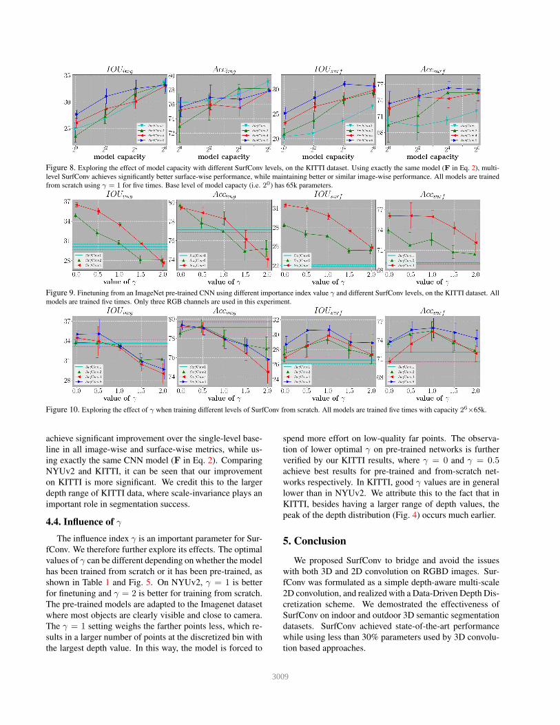
Figure 8. Exploring the effect of model capacity with different SurfConv levels, on the KITTI dataset. Using exactly the same model (F in Eq. 2), multi-
level SurfConv achieves significantly better surface-wise performance, while maintaining better or similar image-wise performance. All models are trained
from scratch using γ = 1 for five times. Base level of model capacty (i.e. 20) has 65k parameters.
Figure 9. Finetuning from an ImageNet pre-trained CNN using different importance index value γ and different SurfConv levels, on the KITTI dataset. All
models are trained five times. Only three RGB channels are used in this experiment.
Figure 10. Exploring the effect of γ when training different levels of SurfConv from scratch. All models are trained five times with capacity 26×65k.
achieve significant improvement over the single-level base-
line in all image-wise and surface-wise metrics, while us-
ing exactly the same CNN model (F in Eq. 2). Comparing
NYUv2 and KITTI, it can be seen that our improvement
on KITTI is more significant. We credit this to the larger
depth range of KITTI data, where scale-invariance plays an
important role in segmentation success.
4.4. Influence of γ
The influence index γ is an important parameter for Sur-
fConv. We therefore further explore its effects. The optimal
values of γ can be different depending on whether the model
has been trained from scratch or it has been pre-trained, as
shown in Table 1 and Fig. 5. On NYUv2, γ = 1 is better
for finetuning and γ = 2 is better for training from scratch.
The pre-trained models are adapted to the Imagenet dataset
where most objects are clearly visible and close to camera.
The γ = 1 setting weighs the farther points less, which re-
sults in a larger number of points at the discretized bin with
the largest depth value. In this way, the model is forced to
spend more effort on low-quality far points. The observa-
tion of lower optimal γ on pre-trained networks is further
verified by our KITTI results, where γ = 0 and γ = 0.5achieve best results for pre-trained and from-scratch net-
works respectively. In KITTI, good γ values are in general
lower than in NYUv2. We attribute this to the fact that in
KITTI, besides having a larger range of depth values, the
peak of the depth distribution (Fig. 4) occurs much earlier.
5. Conclusion
We proposed SurfConv to bridge and avoid the issues
with both 3D and 2D convolution on RGBD images. Sur-
fConv was formulated as a simple depth-aware multi-scale
2D convolution, and realized with a Data-Driven Depth Dis-
cretization scheme. We demostrated the effectiveness of
SurfConv on indoor and outdoor 3D semantic segmentation
datasets. SurfConv achieved state-of-the-art performance
while using less than 30% parameters used by 3D convolu-
tion based approaches.
3009

References
[1] D. Boscaini, J. Masci, E. Rodola, and M. Bronstein. Learn-
ing shape correspondence with anisotropic convolutional
neural networks. In NIPS, 2016. 2
[2] L.-C. Chen, Y. Yang, J. Wang, W. Xu, and A. L. Yuille. At-
tention to scale: Scale-aware semantic image segmentation.
In CVPR, 2016. 3
[3] X. Chen, K. Kundu, Y. Zhu, H. Ma, S. Fidler, and R. Urtasun.
3d object proposals using stereo imagery for accurate object
class detection. TPAMI, 2017. 2
[4] X. Chen, H. Ma, J. Wan, B. Li, and T. Xia. Multi-view 3d
object detection network for autonomous driving. In CVPR,
2017. 2
[5] A. Dai, A. X. Chang, M. Savva, M. Halber, T. Funkhouser,
and M. Nießner. Scannet: Richly-annotated 3d reconstruc-
tions of indoor scenes. CVPR, 2017. 2
[6] J. Dai, H. Qi, Y. Xiong, Y. Li, G. Zhang, H. Hu, and Y. Wei.
Deformable convolutional networks. In ICCV, 2017. 3, 5, 6,
7
[7] Z. Deng and L. J. Latecki. Amodal detection of 3d objects:
Inferring 3d bounding boxes from 2d ones in rgb-depth im-
ages. In CVPR, 2017. 2
[8] M. Engelcke, D. Rao, D. Z. Wang, C. H. Tong, and I. Posner.
Vote3deep: Fast object detection in 3d point clouds using
efficient convolutional neural networks. In ICRA, 2017. 2, 3
[9] Y. Fang, J. Xie, G. Dai, M. Wang, F. Zhu, T. Xu, and
E. Wong. 3d deep shape descriptor. In CVPR, 2015. 1,
2
[10] L. Ge, H. Liang, J. Yuan, and D. Thalmann. 3d convolutional
neural networks for efficient and robust hand pose estimation
from single depth images. In CVPR, 2017. 2
[11] A. Geiger, P. Lenz, C. Stiller, and R. Urtasun. Vision meets
robotics: The kitti dataset. IJRR, 32(11):1231–1237, 2013.
1, 2, 5, 6, 7
[12] K. Guo, D. Zou, and X. Chen. 3d mesh labeling via deep
convolutional neural networks. TOG, 35(1):3, 2015. 2
[13] S. Gupta, R. Girshick, P. Arbelaez, and J. Malik. Learning
rich features from rgb-d images for object detection and seg-
mentation. In ECCV, 2014. 1, 2, 5, 6
[14] S. Gupta, J. Hoffman, and J. Malik. Cross modal distillation
for supervision transfer. In CVPR, 2016. 5
[15] Z. Hao, Y. Liu, H. Qin, J. Yan, X. Li, and X. Hu. Scale-aware
face detection. In CVPR, 2017. 3
[16] K. He, X. Zhang, S. Ren, and J. Sun. Deep residual learning
for image recognition. In CVPR, 2016. 5
[17] D. Hoiem and S. Savarese. Representations and techniques
for 3d object recognition and scene interpretation. Synthe-
sis Lectures on Artificial Intelligence and Machine Learning,
5(5):1–169, 2011. 2
[18] P. Hu and D. Ramanan. Finding tiny faces. In CVPR, 2017.
3
[19] H. Huang, E. Kalogerakis, and B. Marlin. Analysis and syn-
thesis of 3d shape families via deep-learned generative mod-
els of surfaces. In Computer Graphics Forum, volume 34,
pages 25–38, 2015. 2
[20] J. Huang and S. You. Point cloud labeling using 3d convolu-
tional neural network. In ICPR, 2016. 2
[21] A. E. Johnson and M. Hebert. Using spin images for efficient
object recognition in cluttered 3d scenes. TPAMI, 21(5):433–
449, 1999. 2
[22] E. Kalogerakis, M. Averkiou, S. Maji, and S. Chaudhuri. 3d
shape segmentation with projective convolutional networks.
In CVPR, 2017. 2
[23] K. Kamnitsas, C. Ledig, V. F. Newcombe, J. P. Simpson,
A. D. Kane, D. K. Menon, D. Rueckert, and B. Glocker. Effi-
cient multi-scale 3d cnn with fully connected crf for accurate
brain lesion segmentation. Medical image analysis, 36:61–
78, 2017. 2
[24] A. Krizhevsky, I. Sutskever, and G. E. Hinton. Imagenet
classification with deep convolutional neural networks. In
NIPS, 2012. 1, 2
[25] B. Li, T. Zhang, and T. Xia. Vehicle detection from 3d lidar
using fully convolutional network. arXiv:1608.07916, 2016.
2
[26] Z. Li, Y. Gan, X. Liang, Y. Yu, H. Cheng, and L. Lin. Lstm-
cf: Unifying context modeling and fusion with lstms for rgb-
d scene labeling. In ECCV, 2016. 2
[27] G. Lin, C. Shen, A. van den Hengel, and I. Reid. Efficient
piecewise training of deep structured models for semantic
segmentation. In CVPR, 2016. 3
[28] T.-Y. Lin, P. Dollar, R. Girshick, K. He, B. Hariharan, and
S. Belongie. Feature pyramid networks for object detection.
In CVPR, 2017. 3
[29] J. Long, E. Shelhamer, and T. Darrell. Fully convolutional
networks for semantic segmentation. In CVPR, 2015. 2, 5, 6
[30] J. Masci, D. Boscaini, M. Bronstein, and P. Vandergheynst.
Geodesic convolutional neural networks on riemannian man-
ifolds. In ICCV Workshops, 2015. 2
[31] D. Maturana and S. Scherer. 3d convolutional neural net-
works for landing zone detection from lidar. In ICRA, 2015.
2
[32] S. Orts-Escolano, C. Rhemann, S. Fanello, W. Chang,
A. Kowdle, Y. Degtyarev, D. Kim, P. L. Davidson,
S. Khamis, M. Dou, et al. Holoportation: Virtual 3d tele-
portation in real-time. In UIST, 2016. 1
[33] C. R. Qi, H. Su, K. Mo, and L. J. Guibas. Pointnet: Deep
learning on point sets for 3d classification and segmentation.
In CVPR, 2017. 2, 5, 6, 7
[34] C. R. Qi, H. Su, M. Nießner, A. Dai, M. Yan, and L. J.
Guibas. Volumetric and multi-view cnns for object classi-
fication on 3d data. In CVPR, 2016. 2
[35] C. R. Qi, L. Yi, H. Su, and L. J. Guibas. Pointnet++: Deep
hierarchical feature learning on point sets in a metric space.
In NIPS, 2017. 2
[36] X. Qi, R. Liao, J. Jia, S. Fidler, and R. Urtasun. 3d graph
neural networks for rgbd semantic segmentation. In CVPR,
2017. 2, 6
[37] G. Riegler, A. O. Ulusoys, and A. Geiger. Oct-
net: Learning deep 3d representations at high resolutions.
arXiv:1611.05009, 2016. 2
[38] N. Sedaghat, M. Zolfaghari, and T. Brox. Orientation-
boosted voxel nets for 3d object recognition.
arXiv:1604.03351, 2016. 2
3010
[39] B. Shi, S. Bai, Z. Zhou, and X. Bai. Deeppano: Deep
panoramic representation for 3-d shape recognition. Signal
Processing Letters, 22(12):2339–2343, 2015. 2
[40] N. Silberman, D. Hoiem, P. Kohli, and R. Fergus. Indoor
segmentation and support inference from rgbd images. In
ECCV, 2012. 2, 5, 6
[41] K. Simonyan and A. Zisserman. Very deep con-
volutional networks for large-scale image recognition.
arXiv:1409.1556, 2014. 5
[42] S. Song and J. Xiao. Deep sliding shapes for amodal 3d
object detection in rgb-d images. In CVPR, 2016. 2
[43] S. Song, F. Yu, A. Zeng, A. X. Chang, M. Savva, and
T. Funkhouser. Semantic scene completion from a single
depth image. In CVPR, 2017. 2, 3, 5, 6, 7
[44] H. Su, S. Maji, E. Kalogerakis, and E. Learned-Miller. Multi-
view convolutional neural networks for 3d shape recognition.
In ICCV, 2015. 2
[45] L. P. Tchapmi, C. B. Choy, I. Armeni, J. Gwak, and
S. Savarese. Segcloud: Semantic segmentation of 3d point
clouds. arXiv:1710.07563, 2017. 2, 5, 6, 7
[46] J. Uhrig, N. Schneider, L. Schneider, U. Franke, T. Brox, and
A. Geiger. Sparsity invariant cnns. In 3DV, 2017. 2
[47] S. Wang, M. Bai, G. Mattyus, H. Chu, W. Luo, B. Yang,
J. Liang, J. Cheverie, S. Fidler, and R. Urtasun. Torontocity:
Seeing the world with a million eyes. In ICCV, 2017. 1
[48] S. Wang, L. Luo, N. Zhang, and J. Li. Autoscaler: Scale-
attention networks for visual correspondence. In BMVC,
2017. 3
[49] Z. Wu, S. Song, A. Khosla, F. Yu, L. Zhang, X. Tang, and
J. Xiao. 3d shapenets: A deep representation for volumetric
shapes. In CVPR, 2015. 2
[50] J. Xie, Y. Fang, F. Zhu, and E. Wong. Deepshape: Deep
learned shape descriptor for 3d shape matching and retrieval.
In CVPR, 2015. 2
[51] P. Xu, F. Davoine, J.-B. Bordes, H. Zhao, and T. Denœux.
Multimodal information fusion for urban scene understand-
ing. Machine Vision and Applications, 27(3):331–349, 2016.
7
[52] M. Zaheer, S. Kottur, S. Ravanbakhsh, B. Poczos,
R. Salakhutdinov, and A. Smola. Deep sets. In NIPS, 2017.
2
[53] A. Zeng, S. Song, M. Nießner, M. Fisher, and J. Xiao.
3dmatch: Learning the matching of local 3d geometry in
range scans. In CVPR, 2017. 2
[54] R. Zhang, S. Tang, Y. Zhang, J. Li, and S. Yan. Scale-
adaptive convolutions for scene parsing. In ICCV, 2017. 3
[55] Y. Zhang, M. Bai, P. Kohli, S. Izadi, and J. Xiao. Deepcon-
text: context-encoding neural pathways for 3d holistic scene
understanding. In ICCV, 2017. 2, 3
[56] H. Zhao, J. Shi, X. Qi, X. Wang, and J. Jia. Pyramid scene
parsing network. In CVPR, 2017. 3
[57] B. Zhou, A. Khosla, A. Lapedriza, A. Oliva, and A. Tor-
ralba. Object detectors emerge in deep scene cnns.
arXiv:1412.6856, 2014. 2
3011
Related Documents