Surface-type Classification in Structured Planar ... · iii The recent advancement in sensing, computing and artiﬁcial intelligence, has led to the ...Author: Awk ToPublish Year:

UNIVERSITY OF TECHNOLOGY, SYDNEY

Surface-type Classification in Structured

Planar Environments under Various

Illumination and Imaging Conditions

by

Andrew Wing Keung To

A thesis submitted in partial fulfillment for the

degree of Doctor of Philosophy

in the

Faculty of Engineering and IT

Electrical, Mechanical and Mechatronic Systems Group

Centre for Autonomous Systems

July 2015

Declaration of Authorship

I, Andrew Wing Keung To , declare that this thesis titled, ‘Surface-type Classification in

Structured Planar Environments under Various Illumination and Imaging Conditions’ and

the work presented in it are my own. I confirm that:

� This work was done wholly or mainly while in candidature for a research degree at

this University.

� Where any part of this thesis has previously been submitted for a degree or any

other qualification at this University or any other institution, this has been clearly

stated.

� Where I have consulted the published work of others, this is always clearly attributed.

� Where I have quoted from the work of others, the source is always given. With the

exception of such quotations, this thesis is entirely my own work.

� I have acknowledged all main sources of help.

� Where the thesis is based on work done by myself jointly with others, I have made

clear exactly what was done by others and what I have contributed myself.

Signed:

Date:

i

UNIVERSITY OF TECHNOLOGY, SYDNEY

Abstract

Faculty of Engineering and IT

Electrical, Mechanical and Mechatronic Systems Group

Doctor of Philosophy

by Andrew Wing Keung To

iii

The recent advancement in sensing, computing and artificial intelligence, has led to the

application of robots outside of the manufacturing factory and into field environments. In

order for a field robot to operate intelligently and autonomously, the robot needs to build

an environmental awareness, such as by classifying the different surface-types on a steel

bridge structure. However, it is challenging to classify surface-types from images that are

captured in a structurally complex environment under various illumination and imaging

conditions. This is because colour and texture features extracted from these images can

be inconsistent.

This thesis presents a surface-type classification approach to classify surface-types in a

structurally complex three-dimensional (3D) environment under various illumination and

imaging conditions. The approach proposes RGB-D sensing to provide each pixel in an

image with additional depth information that is used by two developed algorithms. The

first algorithm uses the RGB-D information along with a modified reflectance model to

extract colour features for colour-based classification of surface-types. The second

algorithm uses the depth information to calculate a probability map for the pixels being

a specific surface-type. The probability map can identify the image regions that have a

high probability of being accurately classified by a texture-based classifier.

A 3D grid-based map is generated to combine the results produced by colour-based

classification and texture-based classification. It is suggested that a robot manipulator is

used to position an RGB-D sensor package in the complex environments to capture the

RGB-D images. In this way, the 3D position of each pixel is precisely known in a

common global frame (robot base coordinate frame) and can be combined using a

grid-based map to build up a rich awareness of the surrounding complex environment.

A case study is conducted in a laboratory environment using a six degree-of-freedom robot

manipulator equipped with a RGB-D sensor package mounted to the end effector. The

results show that the proposed surface-type classification approach provides an improved

solution for vision-based classification of surface-types in a complex structural environment

with various illumination and imaging conditions.

Acknowledgements

I would like to thank my supervisors Prof. Dikai Liu, and Dr Gavin Paul for their continual

support and assistance throughout the course of my research. Your guidance and countless

hours spent towards improving my research work has led to a more complete, quality thesis.

Thanks to the rest of the team at the Centre of Autonomous Systems, and Prof. Gamini

Dissanayake, the head of the research centre, for providing an excellent environment that

has facilitated great research interactions and exchange of ideas. Fellow research student

Gibson Hu for providing encouragement and support throughout the course of the

candidature.

I would finally like to thank my immediate family members Nelson To, Anita Luk, Anson

To, grandparents and Ayesha Tang for believing in me to strive to do my very best.

This work is supported in part by the ARC Linkage Project: A robotic system for steel

bridge maintenance, the Centre for Autonomous Systems (CAS), the NSW Roads and

Maritime Services (RMS) and the University of Technology, Sydney (UTS).

iv

Contents

Declaration of Authorship i

Abstract ii

Acknowledgements iv

List of Figures viii

List of Tables xiii

Abbreviations xiv

Nomenclature xv

Glossary of Terms xix

1 Introduction 1

1.1 Background . . . . . . . . . . . . . . . . . . . . . . . . . . . . . . . . . . . . 3

1.2 Motivation . . . . . . . . . . . . . . . . . . . . . . . . . . . . . . . . . . . . 5

1.3 Scope . . . . . . . . . . . . . . . . . . . . . . . . . . . . . . . . . . . . . . . 6

1.4 Contributions . . . . . . . . . . . . . . . . . . . . . . . . . . . . . . . . . . . 7

1.5 Publications . . . . . . . . . . . . . . . . . . . . . . . . . . . . . . . . . . . . 8

1.5.1 Journal Papers . . . . . . . . . . . . . . . . . . . . . . . . . . . . . . 8

1.5.2 Conference Papers . . . . . . . . . . . . . . . . . . . . . . . . . . . . 8

1.6 Thesis Outline . . . . . . . . . . . . . . . . . . . . . . . . . . . . . . . . . . 9

2 Review of Related Work 11

2.1 Environmental Awareness . . . . . . . . . . . . . . . . . . . . . . . . . . . . 11

2.2 Sensor Technologies and Sensing Approaches Used for Surface Inspection . 16

2.3 Vision-based Classification of Surface(s) with Non-uniform Illumination . . 20

2.4 Vision-based Classification of Surface(s) with Texture Inconsistency . . . . 25

2.5 Discussion . . . . . . . . . . . . . . . . . . . . . . . . . . . . . . . . . . . . . 27

3 Surface-type Classification Approach 30

v

Contents vi

3.1 Surface-type Classification Approach . . . . . . . . . . . . . . . . . . . . . . 31

3.2 Positioning of the RGB-D Sensor Package Using a Robot Manipulator . . . 32

3.3 Calculating the Viewing Distance and Viewing Angle for an Image Pixel . . 34

3.4 Surface-type Map in 3D . . . . . . . . . . . . . . . . . . . . . . . . . . . . . 37

3.4.1 Combined Surface-type Map . . . . . . . . . . . . . . . . . . . . . . 38

3.5 Colour Feature Extraction . . . . . . . . . . . . . . . . . . . . . . . . . . . . 39

3.6 Classification Results Assessment . . . . . . . . . . . . . . . . . . . . . . . . 39

3.7 Discussion . . . . . . . . . . . . . . . . . . . . . . . . . . . . . . . . . . . . . 40

4 Algorithm for Extraction of Colour Features 41

4.1 Chapter 4 Overview . . . . . . . . . . . . . . . . . . . . . . . . . . . . . . . 42

4.2 Diffused Reflectance Values Extraction . . . . . . . . . . . . . . . . . . . . . 45

4.2.1 Torrance-Sparrow Reflectance Model . . . . . . . . . . . . . . . . . . 46

4.2.2 Radiometric Response Function of a Camera . . . . . . . . . . . . . 48

4.2.3 Camera-to-Light Source Position Calculation . . . . . . . . . . . . . 50

4.2.4 Diffused Reflectance Value Calculation - Proposed Colour Features . 53

4.3 CIELab L*a*b* Colour-Space Conversion . . . . . . . . . . . . . . . . . . . 54

4.4 Experiment 1: Surface-type Classification of Images Containing a SingleSurface Plane with Non-uniform Illumination . . . . . . . . . . . . . . . . . 58

4.5 Experiment 2: Surface-type Classification of an Image Containing MultipleSurface Planes with Non-uniform Illumination . . . . . . . . . . . . . . . . . 66

4.6 Discussion . . . . . . . . . . . . . . . . . . . . . . . . . . . . . . . . . . . . . 71

5 Algorithm for Classification Result Assessment 73

5.1 Algorithm Overview . . . . . . . . . . . . . . . . . . . . . . . . . . . . . . . 74

5.2 Image Capture Conditions . . . . . . . . . . . . . . . . . . . . . . . . . . . . 76

5.2.1 Focus Quality . . . . . . . . . . . . . . . . . . . . . . . . . . . . . . . 77

5.2.2 Effect of Focus Quality on Texture Features . . . . . . . . . . . . . . 79

5.2.3 Spatial Resolution . . . . . . . . . . . . . . . . . . . . . . . . . . . . 82

5.2.4 Effect of Spatial Resolution on Texture Features . . . . . . . . . . . 84

5.2.5 Perspective Distortion . . . . . . . . . . . . . . . . . . . . . . . . . . 86

5.2.6 Effect of Perspective Distortion on Texture Features . . . . . . . . . 87

5.3 Calculation of a Probability Map . . . . . . . . . . . . . . . . . . . . . . . . 89

5.4 Experiments . . . . . . . . . . . . . . . . . . . . . . . . . . . . . . . . . . . . 93

5.4.1 Experiment 1: Effect of Image Capture Conditions on Texture Features 94

5.4.2 Experiment 2: Effect of Image Capture Conditions on Surface-typeClassification . . . . . . . . . . . . . . . . . . . . . . . . . . . . . . . 101

5.4.3 Experiment 3: Identification of Accurately Classified Image Region(s)108

5.5 Discussion . . . . . . . . . . . . . . . . . . . . . . . . . . . . . . . . . . . . . 113

6 Case Study 115

6.1 Experiment Setup . . . . . . . . . . . . . . . . . . . . . . . . . . . . . . . . 115

6.1.1 Setup of RGB-D Sensor Package . . . . . . . . . . . . . . . . . . . . 115

6.1.2 Robot Manipulator . . . . . . . . . . . . . . . . . . . . . . . . . . . . 116

6.1.3 Calibration . . . . . . . . . . . . . . . . . . . . . . . . . . . . . . . . 117

Contents vii

6.1.4 Method to Evaluate the Accuracy of Classification Results using aSurface-type Map . . . . . . . . . . . . . . . . . . . . . . . . . . . . . 121

6.1.5 Training Surface-type Classifiers . . . . . . . . . . . . . . . . . . . . 123

6.2 Experiment 1: Surface-type Classification with Viewing Distance Change . 127

6.3 Experiment 2: Surface-type Classification with Viewing Distance andViewing Angle Change . . . . . . . . . . . . . . . . . . . . . . . . . . . . . . 134

6.4 Discussion . . . . . . . . . . . . . . . . . . . . . . . . . . . . . . . . . . . . . 141

7 Conclusions 143

7.1 Summary of Contributions . . . . . . . . . . . . . . . . . . . . . . . . . . . . 143

7.1.1 A Surface-type Classification Approach using RGB-D Images . . . . 143

7.1.2 An Algorithm for Colour Feature Extraction . . . . . . . . . . . . . 144

7.1.3 An Algorithm for Classification Result Assessment . . . . . . . . . . 144

7.1.4 Practical Contribution . . . . . . . . . . . . . . . . . . . . . . . . . . 145

7.2 Discussion of Limitations . . . . . . . . . . . . . . . . . . . . . . . . . . . . 146

7.3 Future Work . . . . . . . . . . . . . . . . . . . . . . . . . . . . . . . . . . . 148

Appendices 149

A IR Camera Hand-eye Calibration 150

A.1 Methodologies . . . . . . . . . . . . . . . . . . . . . . . . . . . . . . . . . . . 150

A.2 Feature Points Identification . . . . . . . . . . . . . . . . . . . . . . . . . . . 151

A.3 Camera-to-robot Transform through 3D Feature Matching . . . . . . . . . . 153

A.4 Hand-Eye Transform and Point Cloud Registration . . . . . . . . . . . . . . 154

A.5 Limitations and Concluding Note . . . . . . . . . . . . . . . . . . . . . . . . 155

B Texture Features 156

B.1 Grey Level Co-occurrence Matrix . . . . . . . . . . . . . . . . . . . . . . . . 156

B.2 Local Binary Patterns . . . . . . . . . . . . . . . . . . . . . . . . . . . . . . 157

C Multi-class Surface-type Classifier 159

C.1 Naive Bayes Classifier . . . . . . . . . . . . . . . . . . . . . . . . . . . . . . 159

C.2 Support Vector Machines . . . . . . . . . . . . . . . . . . . . . . . . . . . . 160

D Surface Preparation Guideline 161

D.1 Description . . . . . . . . . . . . . . . . . . . . . . . . . . . . . . . . . . . . 161

E Confusion Matrices 164

E.1 Chapter 4: Experiment 1 . . . . . . . . . . . . . . . . . . . . . . . . . . . . 164



Bibliography 185

List of Figures

1.1 a) Mock robotic inspection setup in a laboratory; b) Actual bridgemaintenance environment . . . . . . . . . . . . . . . . . . . . . . . . . . . . 2

1.2 a) A sealed containment area established for bridge maintenance; b) Amobile robotic system deployed for steel bridge maintenance . . . . . . . . . 5

2.1 3D geometric map with additional colour information [1] . . . . . . . . . . . 14

2.2 3D scene labelling results for three complex scenes, where: bowl is red, capis green, cereal box is blue, coffee mug is yellow and soda can is cyan [2] . . 16

2.3 Commercial surface inspection instruments [3], please refer to Appendix Dfor SSPC visual guide . . . . . . . . . . . . . . . . . . . . . . . . . . . . . . 17

2.4 Automation of the marble quality classification process: from imageacquisition to the pallets [4] . . . . . . . . . . . . . . . . . . . . . . . . . . . 19

2.5 Directional light source and camera mounted to the end-effector of a bridgemaintenance robot to inspect for rust and grit-blasting quality [5] [6] [7] . . 19

2.6 Images captured with uniform illumination [8][9][10] . . . . . . . . . . . . . 21

2.7 Rust classification results for an original image, and an image with simulatednon-uniform illumination; Rust percentage = percentage of pixels in animage identified as rust [11] . . . . . . . . . . . . . . . . . . . . . . . . . . . 23

2.8 Captured sample image (left), Classification based on single image (middle),Classification based on Hemispherical Harmonic coefficients (right) [12] . . . 25

2.9 Rusty signpost image [13] . . . . . . . . . . . . . . . . . . . . . . . . . . . . 27

3.1 Overview of the proposed surface-type classification approach . . . . . . . . 32

3.2 Coordinate frames of a robot manipulator and an RGB-D sensor package . 33

3.3 Viewing distance and viewing angle for a surface point in 3D . . . . . . . . 34

3.4 The surface normal calculated for a 3D point . . . . . . . . . . . . . . . . . 36

3.5 A grid-based 3D surface-type map used to represent surface-typeclassification results . . . . . . . . . . . . . . . . . . . . . . . . . . . . . . . 37

4.1 Robot manipulator with a directional light source illuminating a surface . . 41

4.2 Colour feature extraction algorithm . . . . . . . . . . . . . . . . . . . . . . . 44

4.3 Diffused and specular reflection . . . . . . . . . . . . . . . . . . . . . . . . . 46

4.4 Parameters of light reflectance model . . . . . . . . . . . . . . . . . . . . . . 47

4.5 Response functions of several different imaging systems [14] . . . . . . . . . 49

viii

List of Figures ix

4.6 a) Greyscale of the calibration image Ωc; b) Binary image of specularreflectance region in the calibration image Ωcs; c) Diffused reflectanceregion in the calibration image Ωcd . . . . . . . . . . . . . . . . . . . . . . . 50

4.7 Light source direction vector estimation using specular centroid pixel . . . . 51

4.8 Calculating θl and dl for a 3D point representing an ith image pixel . . . . . 53

4.9 a) Original image; b) Image adjusted to simulate illumination by a sidedirectional light source; c) Image adjusted to simulate illumination by alight source directly in front of the image plane . . . . . . . . . . . . . . . . 56

4.10 Histograms of colour-space components for image adjusted to simulateillumination by a side directional light source . . . . . . . . . . . . . . . . . 57

4.11 Histograms of colour-space components for image adjusted to simulateillumination by a light source directly in front of the image plane . . . . . . 57

4.12 Experiment environment from which the four surface-types are collected . . 59

4.13 RGB-D sensor package consisting of a Kinect, Point Grey Firefly cameraand LED light source . . . . . . . . . . . . . . . . . . . . . . . . . . . . . . . 60

4.14 The different RGB-D image capture positions used to collect images undernon-uniform illumination . . . . . . . . . . . . . . . . . . . . . . . . . . . . . 60

4.15 Training image and three test images . . . . . . . . . . . . . . . . . . . . . . 61

4.16 Painted surface classification results . . . . . . . . . . . . . . . . . . . . . . 64

4.17 Timber surface classification results . . . . . . . . . . . . . . . . . . . . . . . 64

4.18 Rusted surface classification results . . . . . . . . . . . . . . . . . . . . . . . 65

4.19 Blasted surface classification results . . . . . . . . . . . . . . . . . . . . . . 65

4.20 a) Experiment 2 image that contains two surface planes and threesurface-types; b) Depth image showing the segmented surface planes . . . . 69

4.21 Binary ground truth labelled images for each surface-type. White is thesurface-type, black is not the surface-type . . . . . . . . . . . . . . . . . . . 69

4.22 a) Classification result using RGB features; b) Classification result usinga*b* features; c) Classification result using Kd features. The colour schemeused in these figures are: teal = timber surface, yellow = rusted surface,and red = blasted surface . . . . . . . . . . . . . . . . . . . . . . . . . . . . 69

4.23 Additional images collected in the environment . . . . . . . . . . . . . . . . 70

5.1 Algorithm to calculate a probability map of image pixels being a specificsurface-type . . . . . . . . . . . . . . . . . . . . . . . . . . . . . . . . . . . . 75

5.2 Plane of focus and depth-of-field diagram . . . . . . . . . . . . . . . . . . . 78

5.3 a) Ideal pixel surface position within the DOF range; b) Pixel surfacepositions at the limits of the DOF range . . . . . . . . . . . . . . . . . . . . 78

5.4 Checkerboard image Ωt(u, v) . . . . . . . . . . . . . . . . . . . . . . . . . . 79

5.5 Gaussian blurred images of the checkerboard . . . . . . . . . . . . . . . . . 81

5.6 Box plot diagrams of the texture feature distribution extracted from theblurred images produced using different values of βg . . . . . . . . . . . . . 81

5.7 Example of pixel density on a surface relative to the viewing distance . . . 83

5.8 Upscale and downscale images of the checkerboard image to simulate changein spatial resolution when using a fixed pixel window size to extract texturefeatures . . . . . . . . . . . . . . . . . . . . . . . . . . . . . . . . . . . . . . 85

List of Figures x

5.9 Box plot diagrams of the texture feature distribution extracted from thescaled images produced using different values of βs . . . . . . . . . . . . . . 85

5.10 a) The camera viewing angle used to capture the training dataset, θt, andthe viewing angle threshold, τθ; b) An example of a camera viewing anglethat is within the viewing angle threshold . . . . . . . . . . . . . . . . . . . 87

5.11 Distorted images of the checkerboard . . . . . . . . . . . . . . . . . . . . . . 88

5.12 Box plot diagrams of the texture feature distribution extracted from thedistorted images produced using different values of βk . . . . . . . . . . . . 89

5.13 Sigmoid function to calculate the probability value of a pixel based on theviewing distance . . . . . . . . . . . . . . . . . . . . . . . . . . . . . . . . . 90

5.14 Sigmoid function to calculate the probability value of a pixel based on theviewing angle . . . . . . . . . . . . . . . . . . . . . . . . . . . . . . . . . . . 91

5.15 Visualisation of the probability value Pdc,θc with image capture conditionchanges in viewing distance dc, and viewing angle θc . . . . . . . . . . . . . 92

5.16 Procedure for calculating the probability value of the classification resultsof an image . . . . . . . . . . . . . . . . . . . . . . . . . . . . . . . . . . . . 93

5.17 Experimental setup of camera to capture images of a surface-type . . . . . . 95

5.18 Image capture conditions used to capture images with focus distance changes 95

5.19 Set of images with focus distance changes . . . . . . . . . . . . . . . . . . . 96

5.20 Box plot diagrams of the texture features distribution extracted from theset of images with focus distance change: horizontal axis shows the images(1–15) corresponding with plane of focus change from (30 mm to 170 mm);and vertical axis shows the values for each texture feature . . . . . . . . . . 96

5.21 Image capture conditions used to capture images with spatial resolutionchanges . . . . . . . . . . . . . . . . . . . . . . . . . . . . . . . . . . . . . . 98

5.22 Set of images with spatial resolution changes . . . . . . . . . . . . . . . . . 98

5.23 Box plot diagrams of the texture feature distribution extracted from the setof images with spatial resolution change: horizontal axis shows the images(1–15) corresponding with viewing distance and plane of focus change from(30–170 mm); and vertical axis shows the texture feature values . . . . . . . 99

5.24 Image capture conditions used to capture images with perspective distortion 100

5.25 Set of images with perspective distortion . . . . . . . . . . . . . . . . . . . . 100

5.26 Box plot diagrams of the texture feature distribution extracted from the setof images with perspective distortion: horizontal axis shows the images 1–5corresponding with viewing angle change from 0◦ to 60◦; and vertical axisshows the values for each texture feature . . . . . . . . . . . . . . . . . . . . 101

5.27 Experimental environment to capture surface-type images with differentimage capture conditions . . . . . . . . . . . . . . . . . . . . . . . . . . . . . 102

5.28 Image capture conditions used to capture a set of images for eachsurface-type in the experimental environment . . . . . . . . . . . . . . . . . 103

5.29 Set of images of blasted metal surface captured with changes in imagecapture conditions . . . . . . . . . . . . . . . . . . . . . . . . . . . . . . . . 103

5.30 Set of images of rusted metal surface captured with changes in image captureconditions . . . . . . . . . . . . . . . . . . . . . . . . . . . . . . . . . . . . . 104

List of Figures xi

5.31 Set of images of timber surface captured with changes in image captureconditions . . . . . . . . . . . . . . . . . . . . . . . . . . . . . . . . . . . . . 104

5.32 The images used in the training dataset with image capture conditions ofdc = 100 mm and θc = 0◦ . . . . . . . . . . . . . . . . . . . . . . . . . . . . 105

5.33 Visualisation of the classification accuracy for the surface-type imagescorresponding to the results presented in Tables 5.1, 5.2 and 5.3 . . . . . . . 107

5.34 The RGB-D sensor package used in this experiment and the experimentscene with multiple surface planes . . . . . . . . . . . . . . . . . . . . . . . 109

5.35 600×600 pixels training image of the timber surface-type . . . . . . . . . . . 109

5.36 Row 1 test images; row 2 classification results of test images; row 3segmented image regions with a high probability of being accuratelyclassified . . . . . . . . . . . . . . . . . . . . . . . . . . . . . . . . . . . . . . 110

6.1 RGB-D sensor package: Firefly camera, Kinect, and LED light source . . . 116

6.2 Denso VM-6083 robot manipulator . . . . . . . . . . . . . . . . . . . . . . . 117

6.3 25 checkerboard images captured by the IR camera (left) and the Fireflycamera (right) for intrinsic and extrinsic calibration . . . . . . . . . . . . . 118

6.4 Extrinsic transformation between the Firefly camera and the IR cameracoordinate frames . . . . . . . . . . . . . . . . . . . . . . . . . . . . . . . . . 118

6.5 IR and depth images used to identify the calibration points to performhand-eye calibration . . . . . . . . . . . . . . . . . . . . . . . . . . . . . . . 119

6.6 Real robot manipulator and a simulation of the robot manipulator with apoint cloud transformed into the robot base coordinate frame . . . . . . . . 120

6.7 Calibration images used to identify the light source position relative to theFirefly camera coordinate frame . . . . . . . . . . . . . . . . . . . . . . . . . 120

6.8 The calibration image perspective projected into 3D and light sourceposition relative to the Firefly camera coordinate frame . . . . . . . . . . . 121

6.9 Setup of the environment to generate a benchmark surface-type map . . . . 122

6.10 Benchmark surface-type map, and surface-type map generated fromclassification results . . . . . . . . . . . . . . . . . . . . . . . . . . . . . . . 123

6.11 1280×960 pixels training images collected for each surface-type . . . . . . . 124

6.12 Training image dataset used to extract features to train surface-type classifiers125

6.13 Experiment 1 setup of the laboratory environment . . . . . . . . . . . . . . 127

6.14 Images collected of the environment . . . . . . . . . . . . . . . . . . . . . . 128

6.15 Classification results using classifier trained with RGB features: Timbersurface is dark blue, painted metal surface is sky blue, rusted metal surfaceis yellow and cardboard is red . . . . . . . . . . . . . . . . . . . . . . . . . . 129

6.16 Classification results using classifier trained with a*b* features: Timbersurface is dark blue, painted metal surface is sky blue, rusted metal surfaceis yellow and cardboard is red . . . . . . . . . . . . . . . . . . . . . . . . . . 130

6.17 Classification results using classifier trained with Kd features: Timbersurface is dark blue, painted metal surface is sky blue, rusted metalsurface is yellow and cardboard is red . . . . . . . . . . . . . . . . . . . . . 130

6.18 Classification results using classifier trained with LBP features: Timbersurface is dark blue, painted metal surface is sky blue, rusted metal surfaceis yellow and cardboard is red . . . . . . . . . . . . . . . . . . . . . . . . . . 131

List of Figures xii

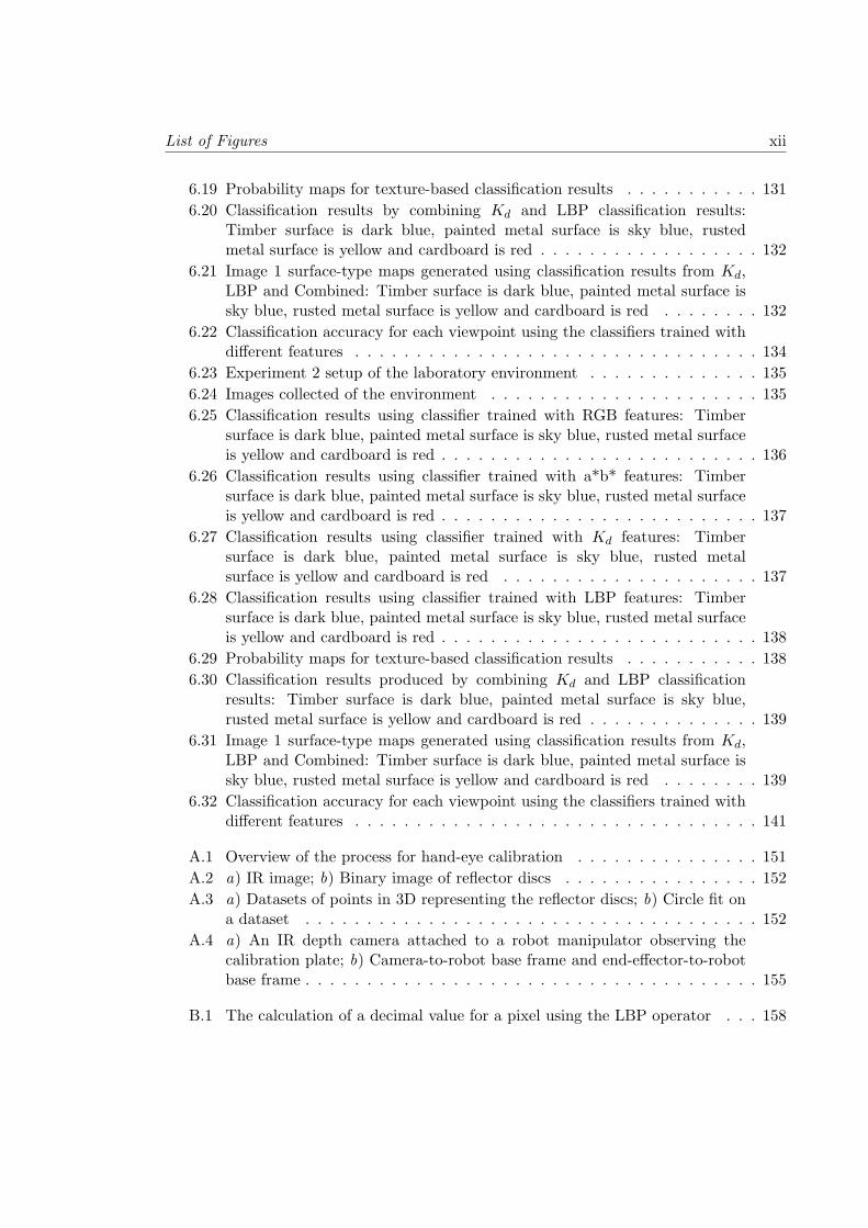
6.19 Probability maps for texture-based classification results . . . . . . . . . . . 131

6.20 Classification results by combining Kd and LBP classification results:Timber surface is dark blue, painted metal surface is sky blue, rustedmetal surface is yellow and cardboard is red . . . . . . . . . . . . . . . . . . 132

6.21 Image 1 surface-type maps generated using classification results from Kd,LBP and Combined: Timber surface is dark blue, painted metal surface issky blue, rusted metal surface is yellow and cardboard is red . . . . . . . . 132

6.22 Classification accuracy for each viewpoint using the classifiers trained withdifferent features . . . . . . . . . . . . . . . . . . . . . . . . . . . . . . . . . 134

6.23 Experiment 2 setup of the laboratory environment . . . . . . . . . . . . . . 135

6.24 Images collected of the environment . . . . . . . . . . . . . . . . . . . . . . 135

6.25 Classification results using classifier trained with RGB features: Timbersurface is dark blue, painted metal surface is sky blue, rusted metal surfaceis yellow and cardboard is red . . . . . . . . . . . . . . . . . . . . . . . . . . 136

6.26 Classification results using classifier trained with a*b* features: Timbersurface is dark blue, painted metal surface is sky blue, rusted metal surfaceis yellow and cardboard is red . . . . . . . . . . . . . . . . . . . . . . . . . . 137

6.27 Classification results using classifier trained with Kd features: Timbersurface is dark blue, painted metal surface is sky blue, rusted metalsurface is yellow and cardboard is red . . . . . . . . . . . . . . . . . . . . . 137

6.28 Classification results using classifier trained with LBP features: Timbersurface is dark blue, painted metal surface is sky blue, rusted metal surfaceis yellow and cardboard is red . . . . . . . . . . . . . . . . . . . . . . . . . . 138

6.29 Probability maps for texture-based classification results . . . . . . . . . . . 138

6.30 Classification results produced by combining Kd and LBP classificationresults: Timber surface is dark blue, painted metal surface is sky blue,rusted metal surface is yellow and cardboard is red . . . . . . . . . . . . . . 139

6.31 Image 1 surface-type maps generated using classification results from Kd,LBP and Combined: Timber surface is dark blue, painted metal surface issky blue, rusted metal surface is yellow and cardboard is red . . . . . . . . 139

6.32 Classification accuracy for each viewpoint using the classifiers trained withdifferent features . . . . . . . . . . . . . . . . . . . . . . . . . . . . . . . . . 141

A.1 Overview of the process for hand-eye calibration . . . . . . . . . . . . . . . 151

A.2 a) IR image; b) Binary image of reflector discs . . . . . . . . . . . . . . . . 152

A.3 a) Datasets of points in 3D representing the reflector discs; b) Circle fit ona dataset . . . . . . . . . . . . . . . . . . . . . . . . . . . . . . . . . . . . . 152

A.4 a) An IR depth camera attached to a robot manipulator observing thecalibration plate; b) Camera-to-robot base frame and end-effector-to-robotbase frame . . . . . . . . . . . . . . . . . . . . . . . . . . . . . . . . . . . . . 155

B.1 The calculation of a decimal value for a pixel using the LBP operator . . . 158

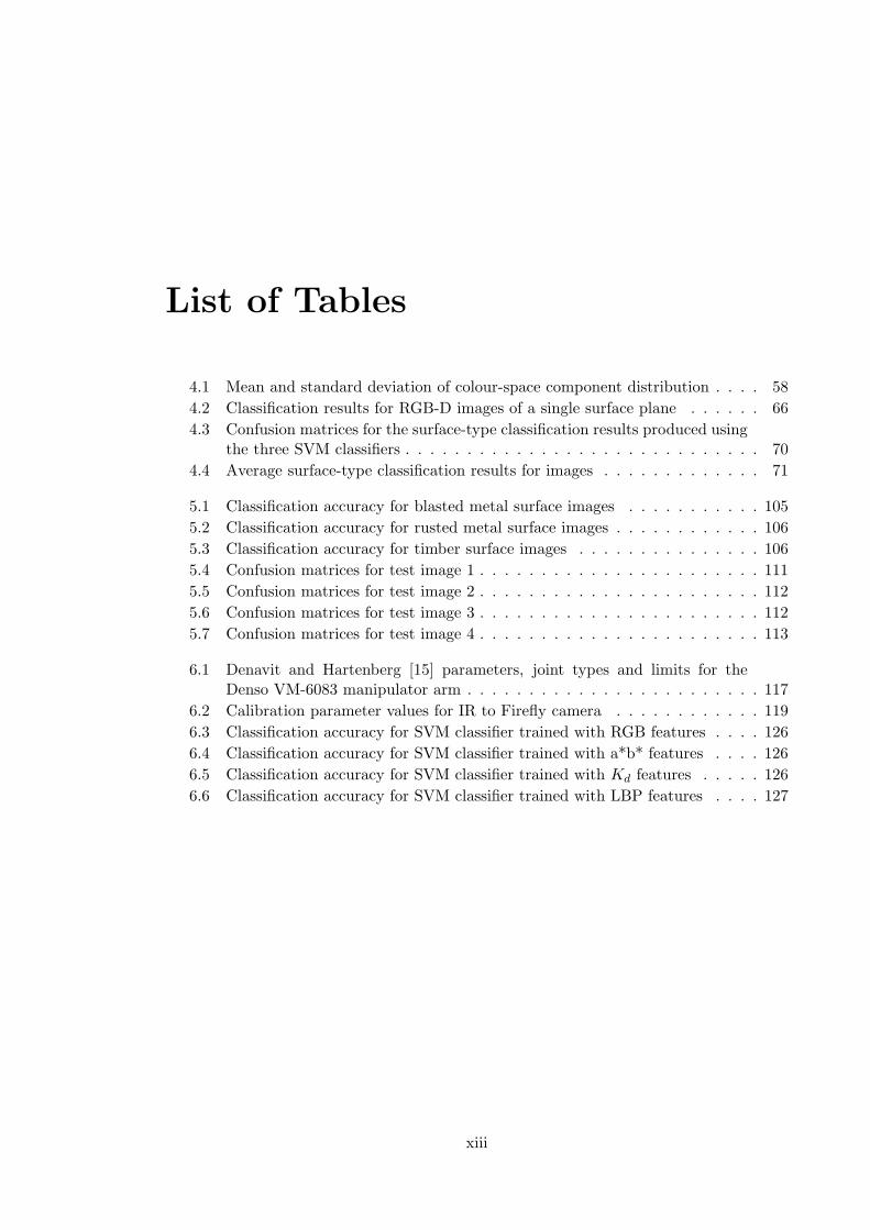
List of Tables

4.1 Mean and standard deviation of colour-space component distribution . . . . 58

4.2 Classification results for RGB-D images of a single surface plane . . . . . . 66

4.3 Confusion matrices for the surface-type classification results produced usingthe three SVM classifiers . . . . . . . . . . . . . . . . . . . . . . . . . . . . . 70

4.4 Average surface-type classification results for images . . . . . . . . . . . . . 71

5.1 Classification accuracy for blasted metal surface images . . . . . . . . . . . 105

5.2 Classification accuracy for rusted metal surface images . . . . . . . . . . . . 106

5.3 Classification accuracy for timber surface images . . . . . . . . . . . . . . . 106

5.4 Confusion matrices for test image 1 . . . . . . . . . . . . . . . . . . . . . . . 111




6.1 Denavit and Hartenberg [15] parameters, joint types and limits for theDenso VM-6083 manipulator arm . . . . . . . . . . . . . . . . . . . . . . . . 117

6.2 Calibration parameter values for IR to Firefly camera . . . . . . . . . . . . 119

6.3 Classification accuracy for SVM classifier trained with RGB features . . . . 126

6.4 Classification accuracy for SVM classifier trained with a*b* features . . . . 126

6.5 Classification accuracy for SVM classifier trained with Kd features . . . . . 126

6.6 Classification accuracy for SVM classifier trained with LBP features . . . . 127

xiii

Abbreviations

DOF Depth of Field

FOV Field of View

GLCM Grey-Level Co-occurrence Matrices

IR Infrared

PCA Principal Component Analysis

RGB-D Red, Green and Blue colour-space image with corresponding Depth

image

SVM Support Vector Machines

UTS University of Technology, Sydney

xiv

Nomenclature

General Formatting Style

f(· · ·) A scalar valued function

f(· · ·) A vector valued function

[· · ·]T Transpose

| · | Absolute value

‖ · ‖ Vector length and normalised vector

C Covariance matrix

d distance between two points

D A diagonalised matrix

i Index value in a list

n Variable signifying the last index of a set or to refer to a count

P Probability

(u, v) Index values in a 2D array or an image

�v A vector

Ω 2D image

τ Threshold

θ Angle between two directional vectors

Specific Symbol Usage

oTe( �Q) Homogenous transformation between the robot base coordinate

frame and the end-effector at pose �Q

oTs Homogenous transformation matrix between the robot base

coordinate frame and the sensor coordinate frame

xv

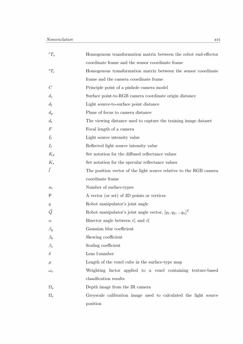
Nomenclature xvi

eTs Homogenous transformation matrix between the robot end-effector

coordinate frame and the sensor coordinate frame

sTc Homogenous transformation matrix between the sensor coordinate

frame and the camera coordinate frame

C Principle point of a pinhole camera model

dc Surface point-to-RGB camera coordinate origin distance

dl Light source-to-surface point distance

dp Plane of focus to camera distance

dt The viewing distance used to capture the training image dataset

F Focal length of a camera

Il Light source intensity value

Ir Reflected light source intensity value

Kd Set notation for the diffused reflectance values

Ks Set notation for the specular reflectance values

�l The position vector of the light source relative to the RGB camera

coordinate frame

nt Number of surface-types

P A vector (or set) of 3D points or vertices

q Robot manipulator’s joint angle

�Q Robot manipulator’s joint angle vector, [q1, q2, ...qn]T

α Bisector angle between �vc and �vl

βg Gaussian blur coefficient

βk Skewing coefficient

βs Scaling coefficient

δ Lens f-number

μ Length of the voxel cube in the surface-type map

ωv Weighting factor applied to a voxel containing texture-based

classification results

Ωs Depth image from the IR camera

Ωc Greyscale calibration image used to calculated the light source

position

Nomenclature xvii

Ωcs An image of the greyscale calibration image Ωc containing the

specular reflectance region

Ωcd An image of the greyscale calibration image Ωc containing the

diffused reflectance region

Ωt A simulated texture pattern image

ϕ Circle of confusion

σ Surface roughness albedo

θc Angle of incidence between the normal of a 3D surface point and

the straight line between the surface point and the RGB camera

coordinate origin

θl Angle of incidence between the normal of a 3D surface point and the

straight line between the surface point and the light source

θt The viewing angle used to capture the training image dataset

τs Pixel intensity threshold for identifying the specular reflectance

region in an image

τd Pixel intensity threshold for identifying the diffused reflectance region

in an image

�vη Normal vector of a 3D surface point

�vc Direction vector between the surface point and the RGB camera

coordinate origin

�vl Direction vector between the light source point and the RGB camera

coordinate origin

P (Mk) Discrete probability distribution of the surface-types for k ∈{1, . . . nt}, given nt number of surface-types.

P (Mk|E) Probability of surface-type state given the evidence E

P (E|Mk) Probability of an evidence given the surface-type

P (E) Probability of evidence

Pdc Probability value of a pixel being a surface-type based on viewing

distance

Pθc Probability value of a pixel being a surface-type based on viewing

angle

Nomenclature xviii

Pdc,θc Probability value of a pixel being a surface-type based on viewing

distance and viewing angle

Combinations of Variables

(a2, a1, a0) Polynomial coefficients for camera radiometric response in the

reflectance model

{Dn1 , Df1} Depth of field threshold range

{Dn2 , Df2} Spatial resolution threshold range

(Kd,R,Kd,G,Kd,B) Diffused reflectance value for each RGB colour channel

(Ks,R,Ks,G,Ks,B) Specular reflectance value for each RGB colour channel

(xc, yc, zc) Axes of RGB camera’s 3D Cartesian coordinate frame

(xo, yo, zo) Axes of Robot base’s 3D Cartesian coordinate frame

(xe, ye, ze) Axes of End-effector’s 3D Cartesian coordinate frame

(xs, ys, zs) Axes of Depth sensor’s 3D Cartesian coordinate frame

(τn, τf , τθ) Threshold parameters to calculate an image pixel’s probability of

being a surface-type

(ω1, ω2) Weighting coefficients to calculate an image pixel’s probability of

being a surface-type

Glossary of Terms

Complex

environment

A 3D workspace that has multiple planar surfaces arranged

in various positions and orientations.

Confusion matrix A specific table that allows the visualisation of classification

results. Each column of the matrix represents the instances

in a predicted class, while each row represents the instances

in an actual class.

Environmental

awareness

In the context for a robot this can include but is not limited

to the knowledge of, a geometric map of the environment

that describes the location of surfaces and obstacles, and a

semantic map that provides a label for objects, surface-types

and locations within the environment.

Grid A type of representation based on occupancy grids used to

divide a space into discrete grid cells. For surface-type map

in 3D this becomes voxels.

Grit-blasting The abrasive removal of surface rust and/or paint using a

high pressure grit stream.

Surface-type map Model of the geometry and surface-type of surfaces in the

environment.

RGB-D The combination of a colour image represented in the RGB

colour-space (red, green, blue) with the addition of depth

data that corresponds with each colour image pixel.

xix

Glossary of Terms xx

Robot manipulator In this thesis, this is a six-degree of freedom Denso industrial

robotic manipulator, with a RGB-D sensor tool mounted on

the end-effector.

Sensor package Generally refers to an IR-based depth sensing camera, a

colour camera and a light source.

Surface The face of an object/structure in the environment.

Surface normal A 3D vector perpendicular to a surface.

Surface-type The appearance of a surface described by the colour and

texture.

Textural appearance The visual appearance of a surface that can be changed by

the image capture conditions.

Viewpoint A position in space and an orientation of a sensor that results

from a manipulator pose �Q. This can also be expressed in

terms of the homogeneous transformation matrix, 0Ts( �Q)

Voxel Volumetric Pixel which represents a 3D cube-like volume in

Euclidean space.

Surface-type Classification in Structured Planar ... · iii The recent advancement in sensing, computing and artiﬁcial intelligence, has led to the ...Author: Awk ToPublish Year:

Documents