Surface roughness and geological mapping at subhectometer scale from the High Resolution Stereo Camera onboard Mars Express

Surface roughness and geological mapping at

sub-hectometer scale from the High

Resolution Stereo Camera onboard Mars

Express

Aurelien Cord a, David Baratoux b, Nicolas Mangold d,

Patrick Martin a, Patrick Pinet b, Ronald Greeley c,

Francois Costard d, Philippe Masson d, Bernard Foing a,

Gerhard Neukum e

aEuropean Space Agency (ESA), ESTEC, RSSD, SCI-SB

Keplerlaan 1, 2201 AZ Noordwijk ZH, The Netherlands

bObservatoire Midi-Pyrenees, UMR5562

14 av. Edouard Belin, 31400 Toulouse, France

cDepartment of Geological Sciences, Arizona State University,

Box 871404, Tempe AZ 85287-1404, USA

dIDES, UMR8148, Bat. 504/509

Universite Paris-Sud, Fac. des sciences, 91405 ORSAY CEDEX, France

eFree University of Berlin, Institute for Geosciences/Planetology,

Malteserstr. 74-100, D-12249 Berlin, Germany

Preprint submitted to ICARUS 9 February 2007

Corresponding Author :

Aurelien Cord

14, passage Dubail

75010 PARIS

FRANCE

+33 6 81 70 55 66

FAX : +33 1 64 69 47 07

[email protected]

Proposed short title :

Surface roughness at sub-hectometer scale from HRSC

2

Abstract

The quantitative measurement of surface roughness of planetary surfaces at all scales

provides insights into geological processes. Complementary of the analysis of local

topographic data of the Martian surface at kilometer scale, as achieved from the

Mars Orbiter Laser Altimeter (MOLA) data, and at the sub-centimeter scale using

photometric properties derived from multi-angular observations, a characterization

of roughness variations at the scale of a few tens of meters is proposed. Relying on a

Gabor filtering process, an algorithm developed in the context of image classification

for the purpose of texture analysis has been adapted to handle data from the High

Resolution Stereo Camera (HRSC). The derivation of roughness within a wavelength

range of tens of meters, combined with analyses at even longer wavelengths, gives an

original view of the Martian surface. The potential of this approach is evaluated for

different examples for which the geological processes are identified and the geological

units are mapped and characterized in terms of roughness.

Key words: Geological Processes, Impact Processes, Image Processing, Mars

Surface, Surface Roughness

Email address: [email protected] (Aurelien Cord).

3

1 Introduction

Fluvial, aeolian or glacial activity, impact cratering and landslides are among

various geological processes which are responsible for roughness variations on

a planetary surface, and particularly on the Martian surface. Such processes

control and/or are controlled by grain or rock sizes and their organization on

the surface. The quantitative measurement of surface roughness at any scale

can provide valuable insights into the characterization of and discrimination

between these geological processes. Earlier studies, based on radar and optical

determination of Mars surface properties, provided the first measurements of

topography variations over scales ranging from centimeters to kilometers. They

demonstrated that the physical properties of the Martian surface vary signif-

icantly and can be used for understanding surface processes (Simpson et al.

1992, Christensen and Moore 1992). More recent investigations (Kreslavsky

and Head 1999, Garvin and Frawley 2000, Kreslavsky and Head 2000, Aharon-

son et al. 2001, Orosei et al. 2003, Neumann et al. 2003) have produced and

analyzed global maps of surface roughness at the sub-kilometer scale or at

longer wavelengths. At sub-millimeter to centimeter scales, the surface topog-

raphy can be investigated by thermal inertia (Putzig et al. 2005, Christensen

et al. 2005) and by photometric measurements (Cord et al. 2003, Pinet et al.

2004, 2005a,b,c, Seelos et al. 2005, Shkuratov et al. 2005, Kreslavsky et al.

2006, Johnson et al. 2006). In a study of Gusev crater, the photometric pa-

rameters correlate with some geological units present in the crater. They are

shown to be very sensitive to particle size (ranging from a few micrometers

to a few centimeters) and their organization on the surface (Jehl et al. 2006,

Pinet et al. 2006). The quantification of the roughness properties at interme-

4

diate scales (i.e., tens of meters) is only recently available for the Martian

surface by photoclinometry (e. g. Kirk et al. (2003), Beyer et al. (2003)), inte-

grative approach (Golombek et al. 2003) and a two-look roughness algorithm

(Mushkin and Gillespie 2005, Adams and Gillespie 2006). We propose in this

work a new method to complete this quantification, through the processing of

any of the images acquired by high spatial resolution imaging devices onboard

current missions (Mars Orbiter Camera / Mars Global Surveyor and HRSC /

Mars Express).

For the sake of clarity in the following, we need to distinguish here between tex-

ture and roughness. Following definitions are for use in this paper only. Rough-

ness characterizes the geometric properties of a surface through a quantitative

parameter describing the intuitive notions of “rough” or “smooth.” The tex-

ture quantifies the homogeneous or heterogeneous aspect of an object within

an image through digital image analysis, and thus is not a surface property

but an image property that relies on the pixel gray-levels in an image. Differ-

ent sources contribute to the texture in an image, including albedo variations,

photometric properties linked to illumination and observation geometries, and

the intrinsic roughness of the surface at a scale of several pixels. The main

point of the approach detailed below is to enhance the latter contribution and

eliminate or reduce the others. As a result, the roughness of geological units

can be inferred at a scale of a few tens of meters.

2 Method

In the context of image classification and segmentation, texture content anal-

ysis has received much attention during the past decades. Relying on the

5

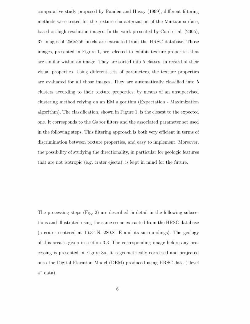
comparative study proposed by Randen and Husoy (1999), different filtering

methods were tested for the texture characterization of the Martian surface,

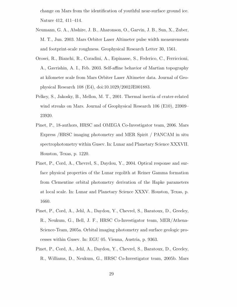
based on high-resolution images. In the work presented by Cord et al. (2005),

37 images of 256x256 pixels are extracted from the HRSC database. Those

images, presented in Figure 1, are selected to exhibit texture properties that

are similar within an image. They are sorted into 5 classes, in regard of their

visual properties. Using different sets of parameters, the texture properties

are evaluated for all those images. They are automatically classified into 5

clusters according to their texture properties, by means of an unsupervised

clustering method relying on an EM algorithm (Expectation - Maximization

algorithm). The classification, shown in Figure 1, is the closest to the expected

one. It corresponds to the Gabor filters and the associated parameter set used

in the following steps. This filtering approach is both very efficient in terms of

discrimination between texture properties, and easy to implement. Moreover,

the possibility of studying the directionality, in particular for geologic features

that are not isotropic (e.g. crater ejecta), is kept in mind for the future.

The processing steps (Fig. 2) are described in detail in the following subsec-

tions and illustrated using the same scene extracted from the HRSC database

(a crater centered at 16.3o N, 280.8o E and its surroundings). The geology

of this area is given in section 3.3. The corresponding image before any pro-

cessing is presented in Figure 3a. It is geometrically corrected and projected

onto the Digital Elevation Model (DEM) produced using HRSC data (“level

4” data).

6

2.1 Preprocessing

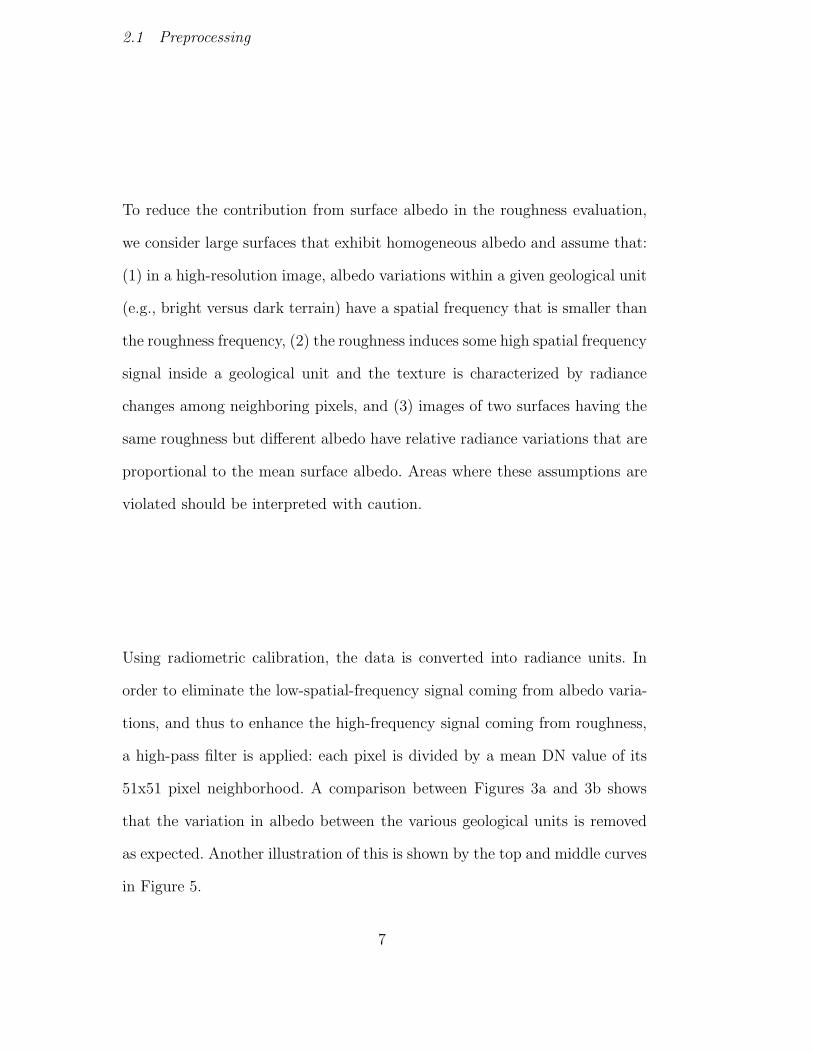
To reduce the contribution from surface albedo in the roughness evaluation,

we consider large surfaces that exhibit homogeneous albedo and assume that:

(1) in a high-resolution image, albedo variations within a given geological unit

(e.g., bright versus dark terrain) have a spatial frequency that is smaller than

the roughness frequency, (2) the roughness induces some high spatial frequency

signal inside a geological unit and the texture is characterized by radiance

changes among neighboring pixels, and (3) images of two surfaces having the

same roughness but different albedo have relative radiance variations that are

proportional to the mean surface albedo. Areas where these assumptions are

violated should be interpreted with caution.

Using radiometric calibration, the data is converted into radiance units. In

order to eliminate the low-spatial-frequency signal coming from albedo varia-

tions, and thus to enhance the high-frequency signal coming from roughness,

a high-pass filter is applied: each pixel is divided by a mean DN value of its

51x51 pixel neighborhood. A comparison between Figures 3a and 3b shows

that the variation in albedo between the various geological units is removed

as expected. Another illustration of this is shown by the top and middle curves

in Figure 5.

7

2.2 Convolution

Gabor filters are first suggested for texture description by Jain and Farrokhnia

(1991). The impulse response h(x, y) can be written:

h(x, y) =1

2πσ2g

e−

x2+y

2

2σ2g e

−2πj(x cos(α)+y sin(α))

p0 . (1)

It corresponds to a sinusoid with a period p0 and an orientation controlled by

α that is modulated by a Gaussian envelope with a scale controlled by the

standard deviation σg.

The Gaussian envelope is the same for all filters: the size of the filters is 29x29

pixels, σg is 0.8x29 pixel. Four orientations (α ∈ [0o, 45o, 90o, 135o] with respect

to the abscissa axis taken as a reference) and three periods characterizing the

spatial scales related to 9, 7 and 4 pixels (p0 ∈ [9, 7, 4] pixels) are selected.

2.3 Local texture estimate

In the next processing step, a local texture estimate is calculated for the

purpose of transforming the filtered areas for which band-pass frequency com-

ponents are strong into a high-constant gray level, and areas for which these

components are weak into a low-constant gray level. The filtered response is

rectified (operation of transforming negative amplitudes into the correspond-

ing positive amplitudes) and smoothed (Weszka et al. 1976).

First, we calculate the magnitude of the outputs from the convolution at

all periods ([9, 7, 4] pixels) and orientations ([0o, 45o, 90o, 135o]). The results

obtained with the 9-pixel scale for the four directions are presented in Figure

4. In order to obtain a local texture estimate regardless of the directionality,

8

the average magnitude based on the orientations is calculated for each value

of the period. Then a low-pass Gaussian filter is applied and for this purpose

we choose a 29x29 pixel filter with a scale parameter (σg) of 0.8x29 pixels.

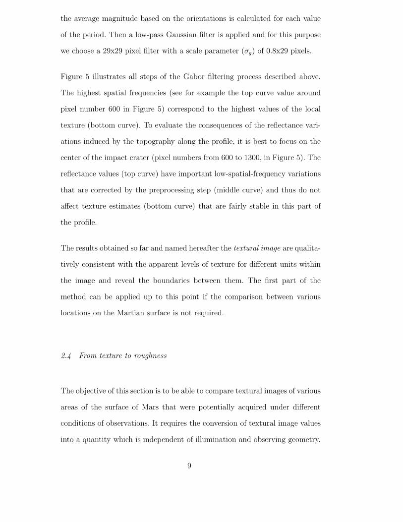
Figure 5 illustrates all steps of the Gabor filtering process described above.

The highest spatial frequencies (see for example the top curve value around

pixel number 600 in Figure 5) correspond to the highest values of the local

texture (bottom curve). To evaluate the consequences of the reflectance vari-

ations induced by the topography along the profile, it is best to focus on the

center of the impact crater (pixel numbers from 600 to 1300, in Figure 5). The

reflectance values (top curve) have important low-spatial-frequency variations

that are corrected by the preprocessing step (middle curve) and thus do not

affect texture estimates (bottom curve) that are fairly stable in this part of

the profile.

The results obtained so far and named hereafter the textural image are qualita-

tively consistent with the apparent levels of texture for different units within

the image and reveal the boundaries between them. The first part of the

method can be applied up to this point if the comparison between various

locations on the Martian surface is not required.

2.4 From texture to roughness

The objective of this section is to be able to compare textural images of various

areas of the surface of Mars that were potentially acquired under different

conditions of observations. It requires the conversion of textural image values

into a quantity which is independent of illumination and observing geometry.

9

In order to obtain such a calibration, we have estimated the texture properties

of synthetic images using the same filtering sequence. The synthetic images

are shaded-relief images from randomly-generated topographic surfaces. Thus,

the texture properties can be linked to the topographic characteristics.

2.4.1 Synthetic textures

Topographic surfaces are generated as random self-affine surfaces. The power

spectrum of the topography, defined as the square of the coefficients in a

Fourier series, has a power law dependence:

|F (l)|2 ∝ |l|β (2)

where F is the Fourier transform of a function representing the elevations, l the

wave number, and β the exponent of the power law. The topographic surfaces

of Venus, Mars, Earth and the Moon all display an exponent value close to 2

at wavelengths greater than a few kilometers (Balmino 1993, Turcotte 1987).

This exponent value corresponds to a Brown noise which is explained in the

case of diffusion processes.

However, at shorter wavelengths there is a tendency toward relatively steeper

slopes or higher values of β (Dodds and Rothman 2000, Weeks et al. 1996).

Here, we assume that the power law with one unique value of the exponent is

valid for the restricted range of scales affecting the textural images obtained

at one given period. Different values of this exponent likely correspond to dif-

ferent geological processes. In this study, the observation angles are systemati-

cally neglected because the images of highest resolution are taken under nadir

conditions (the emergence angle is always smaller than 15 degrees). In order

10

to produce the relationship of β as a function of the texture estimate (i.e.,

the normogram), the following procedure is repeated ten times and results are

averaged for each considered incidence angle.

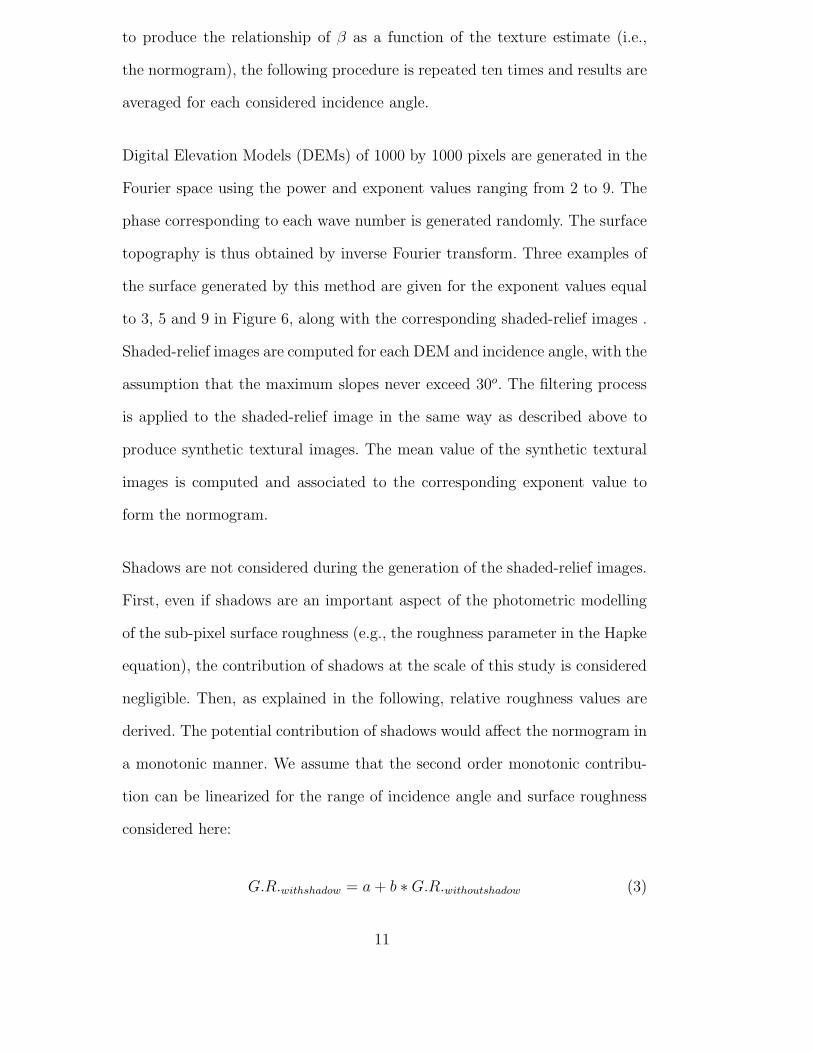
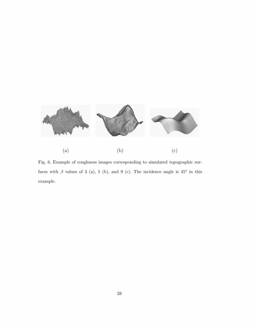
Digital Elevation Models (DEMs) of 1000 by 1000 pixels are generated in the

Fourier space using the power and exponent values ranging from 2 to 9. The

phase corresponding to each wave number is generated randomly. The surface

topography is thus obtained by inverse Fourier transform. Three examples of

the surface generated by this method are given for the exponent values equal

to 3, 5 and 9 in Figure 6, along with the corresponding shaded-relief images .

Shaded-relief images are computed for each DEM and incidence angle, with the

assumption that the maximum slopes never exceed 30o. The filtering process

is applied to the shaded-relief image in the same way as described above to

produce synthetic textural images. The mean value of the synthetic textural

images is computed and associated to the corresponding exponent value to

form the normogram.

Shadows are not considered during the generation of the shaded-relief images.

First, even if shadows are an important aspect of the photometric modelling

of the sub-pixel surface roughness (e.g., the roughness parameter in the Hapke

equation), the contribution of shadows at the scale of this study is considered

negligible. Then, as explained in the following, relative roughness values are

derived. The potential contribution of shadows would affect the normogram in

a monotonic manner. We assume that the second order monotonic contribu-

tion can be linearized for the range of incidence angle and surface roughness

considered here:

G.R.withshadow = a + b ∗ G.R.withoutshadow (3)

11

where G.R. is the response of the image to the Gabor filtering sequence. In

that case, relative estimation of roughness remains valid, even if shadows were

neglected during the process. Because of this assumption, large wall slopes,

or large topographic variations should not be considered by this texture-to-

roughness conversion.

Free parameters exist in the process: the amplitude of the first component

of the spectrum, and the DN amplitudes of the shaded-relief image. It would

have been necessary to introduce a full physical model with the knowledge

of surface albedo, surface scattering properties and instrument calibration in

order to link textural image values to absolute values of β. The process is only

aimed at deriving a corrected value that is independent of the incidence angle.

For this purpose, the free parameters must remain constant (first component

= 1 and DN amplitude = 255). Finally, we translate the exponent into an

equivalent Root Mean Square Slope value (RMSS), as this is a more commonly

used notion in planetary science.

2.4.2 Root Mean Square Slope images

There is a bijection between RMSS values computed at a given scale and β,

meaning that each value of β corresponds to one and only one RMSS value.

The RMSS value is calculated by filtering the surface with a high-pass filter,

through a subtraction by a smoothing filter the size of 10x10 pixels (the size of

this filter is not crucial because the RMSS will be normalized in the following):

RMSS = C ∗

√

1

N

∑

X2 (4)

with N the number of pixels and X corresponding to the difference between

the DEM and the low-pass filtered DEM. C is a constant for the normalization

12

of the RMSS. We choose C (= 103) to force RMSS to be equal to unity within

the ejecta of the impact crater taken as example (Fig. 3a) for the spatial period

associated with the 4-pixel scale (Fig. 7). We then obtain as final result the

RMSS image or model roughness map.

The RMSS value should thus be understood as a relative measure of the true

surface roughness, meaning that a one-to-one correlation exists between our

measure and the true surface roughness. But what matters here the most is

that RMSS maps should be independent of the incidence angle.

2.4.3 Sensitivity analysis of the method

The effect of the assumptions we used in this approach on the final product

cannot be a-priori estimated. We tested the sensitivity of the method by com-

paring textural values from images of the same area under different conditions

of illumination and observation. The two HRSC images were acquired dur-

ing Mars Express orbits 1210 and 1221 at illumination angles of 29o and 20o

and of emergence angles of 12o and 10o, respectively; the spatial resolution

is 13m/pixel in both cases. Figure 8 shows the differences between the two

overlapping textural images and the two overlapping RMSS images, expressed

in percentage of difference (100(V 1−V 2)/V 1 V1 and V2 are respectively the

Digital Number of the first and second image). The mean values for the whole

area and for all spatial periods are in table 1. From these results, it appears

as expected that the texture properties are highly influenced by illumination

conditions (incidence, azimuth). This effect is significantly reduced after filter-

ing and the RMSS values appear much less dependent on the incidence. This

example demonstrates that even with a small angular difference, the texture

13

properties are significantly different while the RMSS values are very similar for

the scene. This approach has not been tested for largely different illumination

conditions and consequently such situations should be approached carefully.

2.5 Synthesis

In summary, our method provides a quantified estimate of the intrinsic local

surface roughness, using calibrated high-resolution images and taking into ac-

count the surface albedo and illumination and observing geometries. Except

when clouds are present (such cases are to be avoided in surface roughness

studies), the atmosphere can be considered homogeneous. Thus, the atmo-

spheric opacity will mainly affect the contrast of the images, and will be elim-

inated during the preprocessing step.

The HRSC technical data assume a global signal-to-noise ratio (SNR) higher

than 100 for panchromatic lines. Since the Gaussian envelope size of Gabor

filters is 29x29 pixels, those filters effectively suppress the highest spatial fre-

quencies and hence suppress a large part of the noise. However, if one deals

with lower SNR data, in particular if the additive components of the noise (e.g.

thermal noise, quantization ?) are important, some noise can be translated

into the roughness map after the preprocessing. As an example, if brighter

and darker surfaces have the same real surface roughness, the processing out-

put will provide with a lower roughness estimate for brighter areas due to the

noise. This additional noise will not necessarily correlate with the geological

units. As a consequence, the potential presence of texture units which are

apparently decorrelated from the ubiquitous geological units seen on a given

image would suggest a dominant noise effect and should call for suspicion.

14

One must bear in mind that the high RMSS values associated with image

edges may result from an edge effect caused by the Gabor filtering and thus

have no physical meaning. Indeed, some leakage of the albedo signal into

roughness estimates is still possible for areas which have strong, high-frequency

albedo variations. Interpretation of roughness estimates should be avoided or

conducted with caution in such areas.

This method could be adapted for roughness estimations with other high-

resolution images (e.g. MOC). That implies to produce normograms to evalu-

ate the roughness obtained at various scales. To compare the results between

them, it may then be worth degrading the spatial resolution of images acquired

at high resolution.

3 Application to geological investigations

This section presents a few examples for which the characterization of the

roughness provides insight into Martian surface geology. The roughness maps

are compiled into RGB composites using the three roughness images of dif-

ferent periods (9, 7 and 4 pixels). The roughness increases from light to dark:

i.e., the lighter the image, the smoother the surface. Bluish color indicates a

higher roughness at large scale and reddish color indicates a higher roughness

at small scale.

3.1 Lobate ejecta craters

Some Martian craters are surrounded by a continuous lobate ejecta blanket

for which the emplacement origin is debated (see, Baratoux et al. (2005) and

15

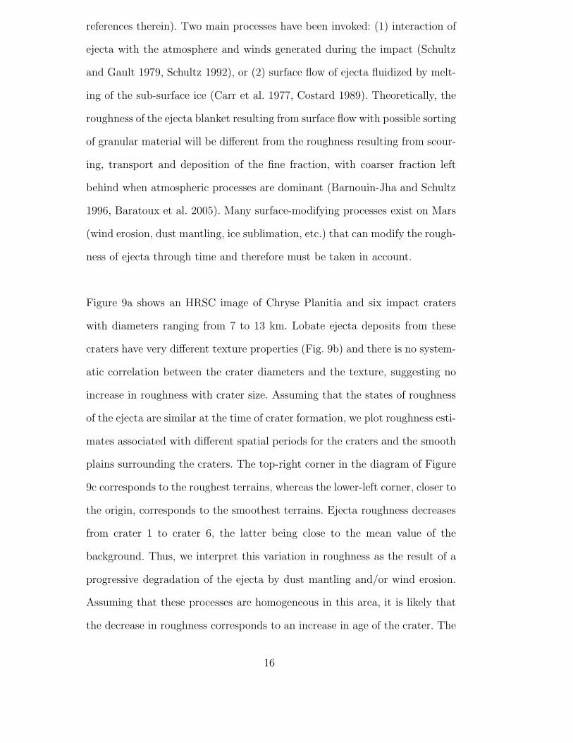
references therein). Two main processes have been invoked: (1) interaction of

ejecta with the atmosphere and winds generated during the impact (Schultz

and Gault 1979, Schultz 1992), or (2) surface flow of ejecta fluidized by melt-

ing of the sub-surface ice (Carr et al. 1977, Costard 1989). Theoretically, the

roughness of the ejecta blanket resulting from surface flow with possible sorting

of granular material will be different from the roughness resulting from scour-

ing, transport and deposition of the fine fraction, with coarser fraction left

behind when atmospheric processes are dominant (Barnouin-Jha and Schultz

1996, Baratoux et al. 2005). Many surface-modifying processes exist on Mars

(wind erosion, dust mantling, ice sublimation, etc.) that can modify the rough-

ness of ejecta through time and therefore must be taken in account.

Figure 9a shows an HRSC image of Chryse Planitia and six impact craters

with diameters ranging from 7 to 13 km. Lobate ejecta deposits from these

craters have very different texture properties (Fig. 9b) and there is no system-

atic correlation between the crater diameters and the texture, suggesting no

increase in roughness with crater size. Assuming that the states of roughness

of the ejecta are similar at the time of crater formation, we plot roughness esti-

mates associated with different spatial periods for the craters and the smooth

plains surrounding the craters. The top-right corner in the diagram of Figure

9c corresponds to the roughest terrains, whereas the lower-left corner, closer to

the origin, corresponds to the smoothest terrains. Ejecta roughness decreases

from crater 1 to crater 6, the latter being close to the mean value of the

background. Thus, we interpret this variation in roughness as the result of a

progressive degradation of the ejecta by dust mantling and/or wind erosion.

Assuming that these processes are homogeneous in this area, it is likely that

the decrease in roughness corresponds to an increase in age of the crater. The

16

older the crater is, the more degraded it becomes. Thus, this example shows

that the variations in roughness might be used to assess the relative age of

craters, a piece of information difficult to access from crater counting on such

a small surface.

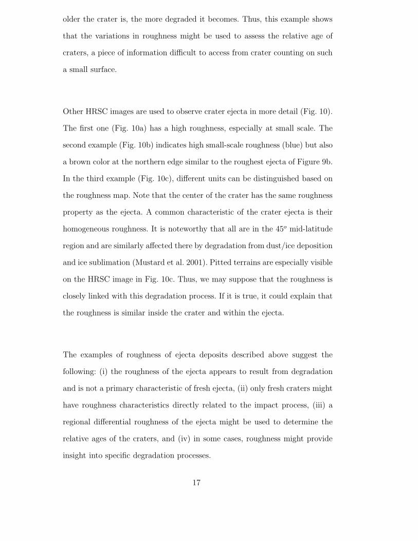
Other HRSC images are used to observe crater ejecta in more detail (Fig. 10).

The first one (Fig. 10a) has a high roughness, especially at small scale. The

second example (Fig. 10b) indicates high small-scale roughness (blue) but also

a brown color at the northern edge similar to the roughest ejecta of Figure 9b.

In the third example (Fig. 10c), different units can be distinguished based on

the roughness map. Note that the center of the crater has the same roughness

property as the ejecta. A common characteristic of the crater ejecta is their

homogeneous roughness. It is noteworthy that all are in the 45o mid-latitude

region and are similarly affected there by degradation from dust/ice deposition

and ice sublimation (Mustard et al. 2001). Pitted terrains are especially visible

on the HRSC image in Fig. 10c. Thus, we may suppose that the roughness is

closely linked with this degradation process. If it is true, it could explain that

the roughness is similar inside the crater and within the ejecta.

The examples of roughness of ejecta deposits described above suggest the

following: (i) the roughness of the ejecta appears to result from degradation

and is not a primary characteristic of fresh ejecta, (ii) only fresh craters might

have roughness characteristics directly related to the impact process, (iii) a

regional differential roughness of the ejecta might be used to determine the

relative ages of the craters, and (iv) in some cases, roughness might provide

insight into specific degradation processes.

17

3.2 Wind streaks

Wind streaks are bright or dark albedo patterns that are often associated

with craters or other topographic features. They are associated with zones of

erosion and deposition induced by wind flows around these obstacles (Sagan

et al. 1973, Greeley and Ivsersen 1985, Tanaka et al. 1992). Most bright streaks

are thought to be deposits of dust in a “shadow zone” characterized by lower

wind speeds. They are thus composed mainly of small-size grains, which could

create a very thin layer (lesser than 1mm) (Pelkey et al. 2001). Such a layer

does not affect the roughness of the surface, as demonstrated in Figure 9b. The

HRSC image of this figure displays many wind streaks which do not appear

on the roughness map, implying that the thickness of wind streaks is small

enough not to affect the roughness at the scale of the measurement (few tens

of meters).

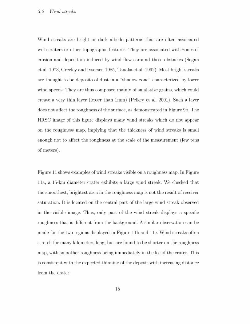
Figure 11 shows examples of wind streaks visible on a roughness map. In Figure

11a, a 15-km diameter crater exhibits a large wind streak. We checked that

the smoothest, brightest area in the roughness map is not the result of receiver

saturation. It is located on the central part of the large wind streak observed

in the visible image. Thus, only part of the wind streak displays a specific

roughness that is different from the background. A similar observation can be

made for the two regions displayed in Figure 11b and 11c. Wind streaks often

stretch for many kilometers long, but are found to be shorter on the roughness

map, with smoother roughness being immediately in the lee of the crater. This

is consistent with the expected thinning of the deposit with increasing distance

from the crater.

18

Different remarks can be drawn from these observations. First, an assumption

of our approach is that there are low-albedo variations within a geological area

of the observed surface (at the scale of tens of meters). If this is true, texture

variations within the image correspond to roughness variations on the ground.

This assumption is not systematically valid, in particular for the dune field

in Figure 11a for which RMSS values are very high and meaningless. Then,

texture and albedo are not directly correlated: the whole bright albedo of

the streak does not correspond to the entire area of smooth texture. Part of

the wind streak shows the same roughness than the surrounding plain, which

is consistent with the presence of a very thin layer of dust which changes

the albedo but not the roughness. Smaller roughness values correspond to a

smoothing induced by the aeolian patterns. This shows that there is a relation

between RMSS values and the thickness of the dust mantling smoothing an

initially rougher surface. Finally, the smoothing is more important closer to

the crater rim, demonstrating the existence of a gradient in dust thickness

from the crater rim to the more distant part of the ejecta blanket where the

roughness of the plain is not modified.

We may expect qualitatively that roughness at the 40-meter scale would re-

quire a thickness of material of a few meters to smooth the surface enough to

be detected. Indeed, initial roughness of the ejecta considered here are similar

and relatively high at this scale in comparison with the surrounding. The effect

would not be visible until the dust thickness is sufficiently large compared to

the surface RMS slope. This explains why some wind streaks are not visible

in the roughness map (Fig. 9b). However, as in Figure 11, when some wind

streaks are visible in the roughness map in comparison with other parts of the

ejecta, the thickness of the deposit needed to produce this smoothing can be

19

evaluated to a few meters. Accurate estimation would require a complete mod-

eling such as done by Forsberg-Taylor et al. (2004). Nevertheless, this result

suggests that the wind streaks consist of thicker dust deposits than previously

supposed, raising the possibility that these streaks formed over long geologic

periods without marked directional changes in the prevailing wind pattern.

The observation of the roughness of wind streaks thus leads to interesting

conclusions about the formation of these features: (i) some wind streaks are

not visible in the roughness map, suggesting a very thin accumulation, whereas

others are detected involving the accumulation of meters of dust. (ii) The entire

streaks seen in the visible image are not seen in the roughness map, suggesting

a gradient in the accumulation of dust from the crater rim to more distant

terrains. (iii) The thickness inferred for the smoothing of the terrains suggests

that wind streaks result from long-term prevailing wind orientations.

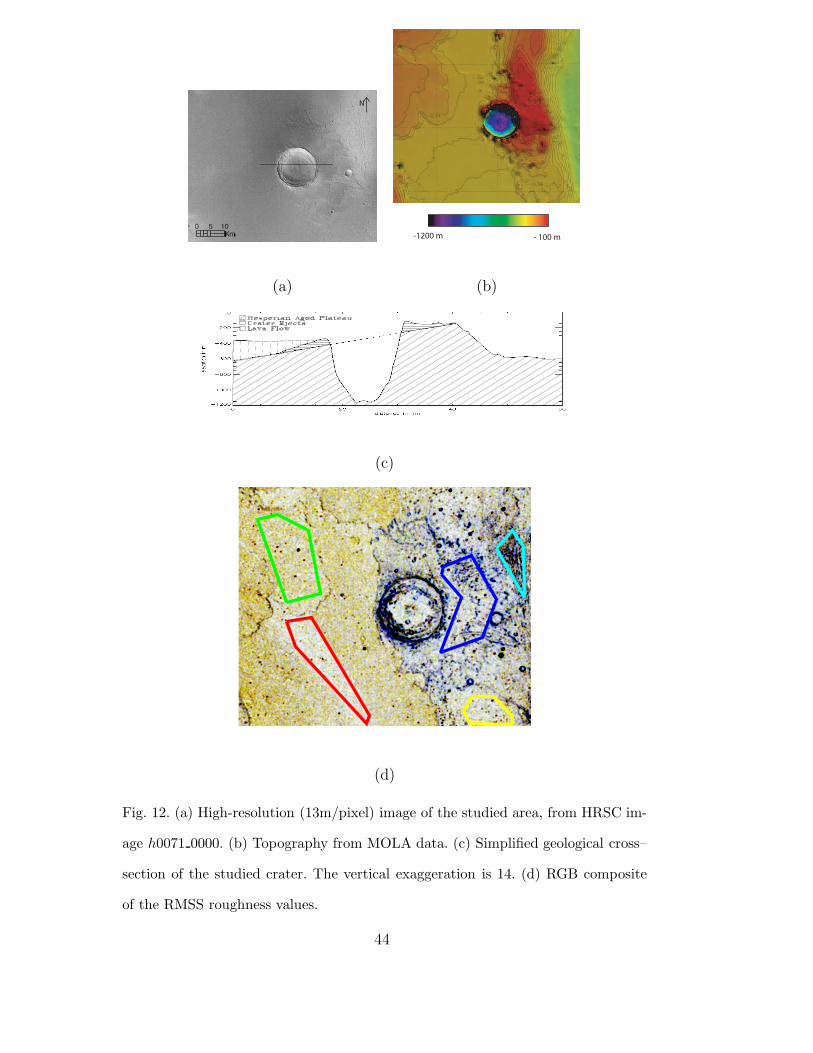
3.3 Lava flows and geological mapping

A region of the northern hemisphere was chosen, based on its different geolog-

ical units and landforms that can be studied and may have different physical

properties (Fig. 12). The geologic map of Scott and Tanaka (1986) shows that

the area is at the junction between the Late Hesperian outflow channel of

Kasei Valles and Amazonian lava flows originating from the Tharsis plateau.

The HRSC image shows overlapping lobate lava flows that have prominent

south-eastern slopes. This is confirmed by MOLA topography which shows

a South-East-oriented gradual slope, to the West of the impact crater (Fig.

12b). The MOLA data also show a topographic plateau to the East of the im-

pact crater with a surface dipping 1.2o to the West. The fact that the crater

20

is situated on this slope explains that the lava flows buried only the western

part of its ejecta (Fig. 12c).

Using the spatial resolution of 13 m/pixel, the pixel size periods (9, 7 and 4

pixels) are converted into meters (120, 90 and 50 m, respectively). Most geo-

logical units visible in the image are very well defined using the roughness map

(Fig. 12d). They are divided into regions of interest (ROI) that we compare to

a reference area, sampled in the plain located South of the crater and repre-

sented in the figure by the yellow polygon. At the extreme East, the very rough

unit as compared to the reference corresponds to striated units of the Kasei

valley floor. A portion of the crater’s ejecta (blue ROI) appears very similar

to the reference at 50 and 90 m, whereas it becomes rougher at the period of

120 m. The same observation is made for most ejecta deposits shown in Figure

9b. At this scale, the rough ejecta surface, inherited from the fragmentation

and emplacement mechanism, seems not to be completely erased by smooth-

ing coming from dust deposition and wind erosion. Lava flows (green ROI)

display a very homogeneous roughness compared to the other units. Most of

them are rougher than the reference (with significant roughness at the 50-m

period), suggesting that the mantling by windblown sediments is too thin to

hide the topography completely. This may result from the younger age of the

lavas relative to the reference. Because the roughness is more important at

50 m than at 120 m, we suggest that the lavas are not composed of large

blocks (several tens of meters large) but rather have a pattern at a few meters

scale related to the cooling of typical fluid lavas. A very smooth area appears

within the lava flows (red ROI). Even when ”stretched” to the extreme, the

HRSC image does not show the same pattern. Such a smooth area could indi-

cate a roughness directly related to the lava flow (e.g., very fluid and smooth

21

pahoehoe-like lavas), or it could reflect a thick dust mantling.

We compared these results with the roughness determined by Kreslavsky and

Head (2000). At the considered 0.6, 2.4 and 9.6 km scales, the roughness of

the ejecta is systematically higher than that of the lava flow. Combining the

two approaches, it appears that above a scale of about 50 m, the ejecta are

systematically rougher than the lava flows, probably because the ejecta layer

is partially, but not totally covered by dust. The dust coverage smoothed first

the small spatial period. A part of the original ejecta is still visible at larger

spatial period.

The examples outlined above suggest that: (i) the roughness map can be used

to contribute to the mapping of geological units not otherwise seen in the

original image, (ii) Martian crater ejecta is rougher than the lava flows in the

studied area, implying that it is possible to distinguish roughness signatures

which are not related to degradation processes.

4 Discussion and Conclusions

Our study provides a method for describing surface roughness at sub-hectometric

scale linked to surface blocks and rock size distribution and organization.

Somehow, it meets conclusions recently reached stating that: (i) careful spec-

tral unmixing of HRSC images reveals that the shade-fraction images con-

tain qualitative information on surface roughness at a subpixel scale (Mc-

Cord et al. 2007); (ii) subpixel surface roughness variations can be quantified

from HRSC by means of two-look approach techniques (Mushkin and Gillespie

2006, Mushkin and Gillespie 2005). The roughness variations derived from the

22

present work can be related to both the state of degradation (e.g., amount

of dust mantling) and/or to its geological properties (e.g., lava flow type).

Combining this information with other data (e.g., topography, high resolution

images, thermal emission) and products (e.g., thermal inertia, macroscopic

roughness, crater count) could be quite fruitful. Frequently, the thermal iner-

tia calculated from THEMIS data is influenced by the upper few decimeters

of the surface and allows for the distinction between rocky and dusty surfaces

(Fergason et al. 2006). Our approach may detect and map the indurated dust

that does not produce typical thermal signatures for fine particles. Such a

combination will be useful for improving the description of the surface state

and its physical modeling.

Moreover, a wide range of applications can be considered which may lead to

a systematic analysis and classification of Martian surface roughness. This

study is based on only a few examples, limiting the following conclusions, but

demonstrates the potentially wide applications of the approach.

The roughness of impact crater ejecta often corresponds to degradation /de-

position processes rather than roughness inherited by the impact process, and

can be used to gain insight into these specific degradation processes and their

timescales.

Regarding lava flows, an observed presence and diversity of roughness varia-

tions could be related either to different states of weathering lava or to various

types of lava.

Regarding feature detection, the roughness map can be used for the mapping

of geological units as well as sub-units not identified in the original image.

Moreover, wrinkle ridges or fractures are highlighted by this algorithm and

23

could be used for a detailed regional mapping of such features, given the

extended coverage of HRSC data.

Regarding age evaluation, variations in roughness of the ejecta may be used

to determine the relative ages of various craters located in the same region.

With the support of a few additional constraints provided by the regional

geologic context, identical roughness associated with different crater ejecta

may indicate the same state of degradation, suggesting identical formation

times.

Regarding aeolian processes, the smoothing of a surface by dust deposition

may be characterized by its roughness properties. Some wind streaks are not

visible on the roughness map, implying a very thin accumulation, whereas

other ones are detected, implying meters-thick accumulation of dust. Such

a thickness suggests that wind streaks are features existing within the same

pattern over geological times and under constant prevailing wind direction.

The derivation of a surface ratio between wind streaks features that are only

detectable from the albedo and features that are seen in the roughness map

could be envisioned as a proxy for deriving quantitative estimates both on

aeolian transport and depositional processes.

Acknowledgment

We thank the HRSC Experiment Teams at Freie Universitt Berlin and DLR

Berlin, as well as the ESA Mars Express Project Teams at ESTEC and

ESOC for the successful planning and acquisition of the imaging data as

well as for making the processed data sets available. We acknowledge the

24

effort of the HRSC Co-Investigator Team members and their associates who

have contributed to this investigation in the preparatory phase and in sci-

entific discussions within the HRSC Team. For this study, the HRSC Ex-

periment Team of the German Aerospace Center (DLR) in Berlin has pro-

vided map-projected HRSC image data, and standard HRSC Digital Eleva-

tion Models. This work was supported by an ESA post-doctoral fellowship

attributed to A. Cord. The research has also benefited from support given

by the French Space Agency CNES and by the PNP (Programme National

de Plantologie) to the Co-Investigator French groups, respectively P.P. and

D.B. at LDTP/UMR 5562/CNRS/ Toulouse University and P.M., N.M., and

F.C. at IDES/UMR 8148/CNRS/Orsay-Paris Sud University. We gratefully

thank Mikhail Kreslavsky, Alan Gillespie and the third anonymous reviewer

for their constructive and thorough comments, which substantially improved

this paper.

References

Adams, J. B., Gillespie, A. R., 2006. Remote Sensing of Landscapes with Spec-

tral Images A Physical Modeling Approach. Cambridge University Press,

Cambridge.

Aharonson, O., Zuber, M. T., Rothman, D., 2001. Statistics of Mars’ topog-

raphy from the Mars Orbiter Laser Altimeter. Journal of Geophysical Re-

search 106, 23723 – 23735.

Balmino, G., 1993. The spectra of the topography of the Earth, Venus and

Mars. Geophysical Research Letters 20 (11), 1063–1066.

Baratoux, D., Mangold, N., Pinet, P., Costard, F., 2005. Thermal proper-

ties of lobate ejecta in Syrtis Major, Mars: Implications for the mech-

25

anisms of formation. Journal of Geophysical Research 110, E04011,

doi:10.1029/2004JE002314.

Barnouin-Jha, O. S., Schultz, P. H., 1996. Ejecta entrainment by impact-

generated ring vortices : Theory and experiments. Journal of Geophysical

Research 101 (E9), 21099–21115.

Beyer, R. A., McEwen, A. S., Kirk, R. L., Dec. 2003. Meter-scale slopes of

candidate MER landing sites from point photoclinometry. Journal of Geo-

physical Research 108 (E12), doi:10.1029/2003JE002120.

Carr, M. H., Crumpler, L., Cutts, J., Greeley, R., Guest, J., Masursky, H.,

1977. Martian impact craters and emplacement of ejecta by surface flow.

Journal of Geophysical Research 82, 4055–4065.

Christensen, P., Moore, H., 1992. The Martian surface layer. In: Mars. Uni-

versity of Arizona Press, Tucson, pp. 686–729.

Christensen, P. R., Gorelick, N., Fergason, R., Dec. 2005. Searching for change

in the Martian night: Investigating nighttime temperature anomalies using

THEMIS. AGU Fall Meeting Abstracts, P24A–01.

Cord, A., Martin, P., Foing, B., Jaumann, R., Hauber, E., Hoffmann, H.,

Neukum, G., HRSC Co-Investigator team, 2005. Martian surface texture

study by a filtering approach using Mars Express HRSC data. In: First

Mars Express Conference. Noordwijk, The Netherlands, p. 138.

Cord, A., Pinet, P. C., Daydou, Y., Chevrel, S., 2003. Planetary regolith sur-

face analogs: Optimized determination of Hapke parameters using multi-

angular spectro-imaging laboratory data. Icarus 165, 414–427.

Costard, F., 1989. The spatial distribution of volatiles in the Martian hy-

drolithosphere. Earth, Moon and Planets 45, 265–290.

Dodds, P. S., Rothman, D., 2000. Scaling, universality, and geomorphology.

Annual Review of Earth and Planetary Sciences 28, 571–610.

26

Fergason, R., Christensen, P., Kieffer, H. H., 2006. High-resolution thermal in-

ertia derived from the Thermal Emission Imaging System (THEMIS): Ther-

mal model and applications. Journal of Geophysical Research E12004 (111),

doi:10.1029/2006JE002735.

Forsberg-Taylor, N. K., Howard, A. D., Craddock, R. A., 2004. Crater degrada-

tion in the Martian highlands: Morphometric analysis of the Sinus Sabaeus

region and simulation modeling suggest fluvial processes. Journal of Geo-

physical Research 109, E05002, doi:10.1029/2004JE002242.

Garvin, J. B., Frawley, J. J., 2000. Global vertical roughness of Mars from Mars

Orbiter Laser Altimeter pulsewidth measurements. In: Lunar and Planetary

Science XXXI. Houston, Texas, p. 1884.

Golombek, M. P., Haldemann, A. F. C., Forsberg-Taylor, N. K., DiMaggio,

E. N., Schroeder, R. D., Jakosky, B. M., Mellon, M. T., Matijevic, J. R., Oct.

2003. Rock size-frequency distributions on Mars and implications for Mars

Exploration Rover landing safety and operations. Journal of Geophysical

Research 108 (E12), 27–1.

Greeley, R., Ivsersen, J., 1985. Wind as a geological process. Cambridge Plan-

etary Sciences series:4. Cambridge University Press.

Jain, A. K., Farrokhnia, F., 1991. Unsupervised texture segmentation using

Gabor filters. Pattern Recognition 24(12), 1167–1186.

Jehl, A., 16 authors, HRSC Co-Investigator team, 2006. Improved surface

photometric mapping across Gusev and Apollinaris from an HRSC/Mars

Express integrated multi-orbit dataset: implication on Hapke parameters

determination. In: Lunar and Planetary Science XXXVII. Houston, Texas,

p. 1219.

Johnson, J., Grundy, W., Lemmon, M., Bell III, J., Johnson, M., Deen, R.,

Arvidson, R., Farrand, W., Guinness, E., Herkenhoff, K., Seelos IV, F.,

27

Soderblom, J., Squyres, S., 2006. Spectrophotometric properties of materials

observed by Pancam on the Mars Exploration Rovers: 1. Spirit. Journal of

Geophysical Research 111 (E02S14), doi:10.1029/2005JE002494.

Kirk, R. L., Barrett, J. M., Soderblom, L. A., 2003. Photoclinometry made

simple? In: Working Group IV/9 , Workshop ”Advances in Planetary Map-

ping 2003”. Houston, Texas.

Kreslavsky, M., Bondarenko, N. V., Pinet, P. C., Raitala, J., Neukum, G.,

MEx-Co-I-team, 2006. Mapping of photometric anomalies of Martian sur-

face with HRSC data. In: Lunar and Planetary Science XXXVII. Houston,

Texas, p. 2211.

Kreslavsky, M. A., Head, J. W., 1999. Kilometer-scale slopes on Mars and their

correlation with geologic units: Initial results from Mars Orbiter Laser Al-

timeter (MOLA) data. Journal of Geophysical Research 104, 21,911–21,924.

Kreslavsky, M. A., Head, J. W., 2000. Kilometer-scale roughness of Mars:

Results from MOLA data analysis. Journal of Geophysical Research 105

(E11), 26,695–26,711.

McCord, T., Adams, J., Bellucci, G., Combes, J., Gillespie, A., Hansen, G.,

Hoffman, H., Jaumann, R., G., N., Pinet, P., Poulet, F., Stephan, K., Group,

T. S. W., HRSC Co-Investigator team, 2007. The Mars Express High Reso-

lution Stereo Camera spectrophotometric data : characteristics and science

analysis. Journal of Geophysical Research in press.

Mushkin, A., Gillespie, A., 2005. Estimating subpixel surface roughness using

remotely sensed stereoscopic data. Remote Sensing environment 99, 75–83.

Mushkin, A., Gillespie, A., 2006. Mapping sub-pixel surface roughness on Mars

using high-resolution satellite image data. Geophysical Research Letters 33,

L18204.1–L18204.6.

Mustard, J. F., Cooper, C. D., Rifkin, M. K., 2001. Evidence for recent climate

28

change on Mars from the identification of youthful near-surface ground ice.

Nature 412, 411–414.

Neumann, G. A., Abshire, J. B., Aharonson, O., Garvin, J. B., Sun, X., Zuber,

M. T., Jun. 2003. Mars Orbiter Laser Altimeter pulse width measurements

and footprint-scale roughness. Geophysical Research Letter 30, 1561.

Orosei, R., Bianchi, R., Coradini, A., Espinasse, S., Federico, C., Ferriccioni,

A., Gavrishin, A. I., Feb. 2003. Self-affine behavior of Martian topography

at kilometer scale from Mars Orbiter Laser Altimeter data. Journal of Geo-

physical Research 108 (E4), doi:10.1029/2002JE001883.

Pelkey, S., Jakosky, B., Mellon, M. T., 2001. Thermal inertia of crater-related

wind streaks on Mars. Journal of Geophysical Research 106 (E10), 23909–

23920.

Pinet, P., 18-authors, HRSC and OMEGA Co-Investigator team, 2006. Mars

Express /HRSC imaging photometry and MER Spirit / PANCAM in situ

spectrophotometry within Gusev. In: Lunar and Planetary Science XXXVII.

Houston, Texas, p. 1220.

Pinet, P., Cord, A., Chevrel, S., Daydou, Y., 2004. Optical response and sur-

face physical properties of the Lunar regolith at Reiner Gamma formation

from Clementine orbital photometry derivation of the Hapke parameters

at local scale. In: Lunar and Planetary Science XXXV. Houston, Texas, p.

1660.

Pinet, P., Cord, A., Jehl, A., Daydou, Y., Chevrel, S., Baratoux, D., Greeley,

R., Neukum, G., Bell, J. F., HRSC Co-Investigator team, MER/Athena-

Science-Team, 2005a. Orbital imaging photometry and surface geologic pro-

cesses within Gusev. In: EGU 05. Vienna, Austria, p. 9363.

Pinet, P., Cord, A., Jehl, A., Daydou, Y., Chevrel, S., Baratoux, D., Greeley,

R., Williams, D., Neukum, G., HRSC Co-Investigator team, 2005b. Mars

29

Express imaging photometry and surface geologic processes at Mars: What

can be monitored within Gusev crater? In: Lunar and Planetary Science

XXXVI. Houston, Texas, p. 1721.

Pinet, P., Daydou, Y., Cord, A., Chevrel, S., Poulet, F., Erard, S., Bibring,

J.-P., Y.Langevin, Melchiorri, R., Bellucci, G., Altieri, F., Arvidson, R.,

HRSC and OMEGA Co-Investigator team, 2005c. Derivation of Mars sur-

face scattering properties from Omega spot pointing observations. In: Lunar

and Planetary Science XXXVI. Houston, Texas, p. 1694.

Putzig, N. E., Mellon, M. T., Kretke, K. A., Arvidson, R. E., 2005. Global

thermal inertia and surface properties of Mars from the MGS mapping mis-

sion. Icarus 173, 325–341.

Randen, T., Husoy, J., 1999. Filtering for texture classication: A comparative

study. IEEE Transactions on Pattern Analysis and Machine Intelligence

21(4), 291–310.

Sagan, C., Toon, O., Gierash, P., 1973. Climate change on Mars. Science 181,

1045–1049.

Schultz, P., 1992. Atmospheric effects on ejecta emplacement. Journal of Geo-

physical Research 97, 13257–13302.

Schultz, P. H., Gault, D. E., 1979. Atmospheric effects on Martian ejecta

emplacement. Journal of Geophysical Research 84 (B13), 7669–7687.

Scott, D., Tanaka, K., 1986. U.S.G.S. I Map 1802 A. In: XXII Lunar and

Planetary Conference. Houston, Texas, pp. 865–866.

Seelos, F. P., Arvidson, R. E., Guinness, E. A., Wolff, M. J., 2005. Radiative

transfer photometric analyses at the Mars Exploration Rover landing sites.

In: Lunar and Planetary Science XXXVI. Houston, Texas, p. 2054.

Shkuratov, Y. G., Stankevich, D. G., Petrov, D. V., Pinet, P. C., Cord, A. M.,

Daydou, Y. H., Chevrel, S. D., 2005. Interpreting photometry of regolith-

30

like surfaces with different topographies: shadowing and multiple scattering.

Icarus 173, 3–15.

Simpson, R., Harmon, J., Zisk, S., Thompson, T., Muhleman, D., 1992. Radar

determination of Mars surface properties. In: Mars. University of Arizona

Press, Tucson, pp. 652–684.

Tanaka, K., Scott, D., Greeley, R., 1992. Global stratigraphy. In: Mars. Uni-

versity of Arizona Press, Tucson, pp. 345–382.

Turcotte, D., 1987. A fractal interpretation of topography and geoid spectra

on the Earth, Moon, Venus and Mars. Journal of Geophysical Research

92 (B4), E597–E601.

Weeks, R. J., Smith, M., Pak, K., Li, W.-H., Gillespie, A., Gustafson, B.,

1996. Surface roughness, radar backscatter, and visible and near-infrared

reflectance in Death Valley, California. Journal of Geophysical Research

101, 23077–23090.

Weszka, J. S., Dyer, C. R., Rosenfeld, A., 1976. A comparative study of texture

measures for terrain classification. IEE Trans. Systems, Man, Cybernetics

6, 269–285.

31

Period 1 2 3

Texture 29 (19) 29 (18) 28 (17)

RMSS 12 (9) 11 (7) 12 (8)

Table 1

Mean value of the difference in percentage between the two overlapping textural

images and the two overlapping RMSS images. Numbers in brackets correspond

two standard deviations.

32

Fig. 1. Images extracted from the HRSC database exhibiting texture properties

similar all along the image. Each line is a cluster corresponding to the best classifi-

cation.

33

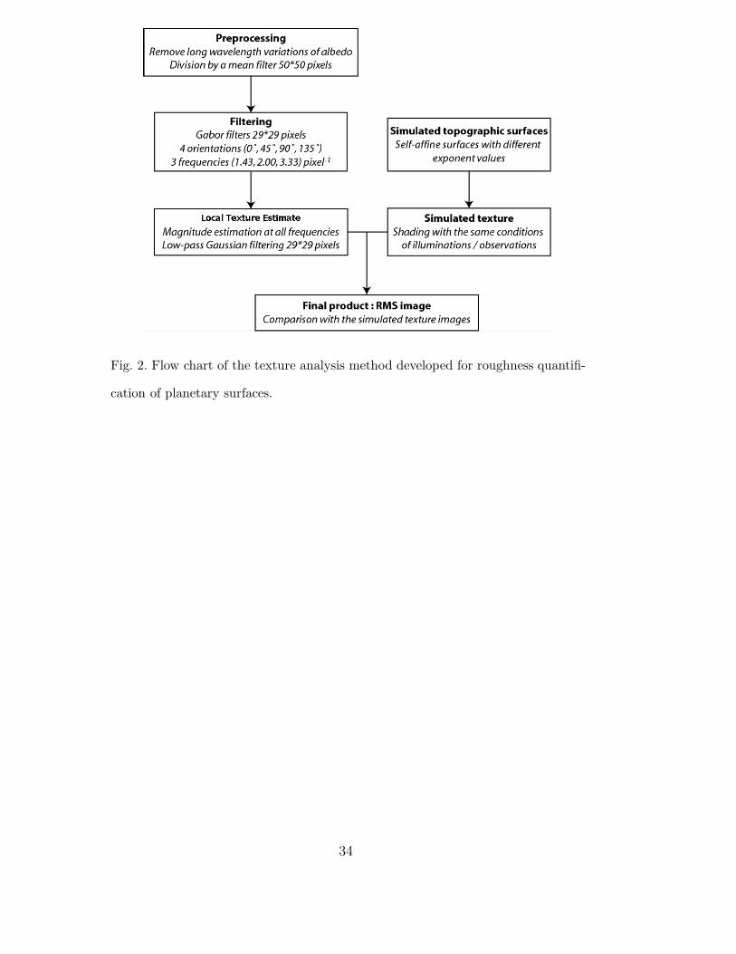
Fig. 2. Flow chart of the texture analysis method developed for roughness quantifi-

cation of planetary surfaces.

34

(a) (b)

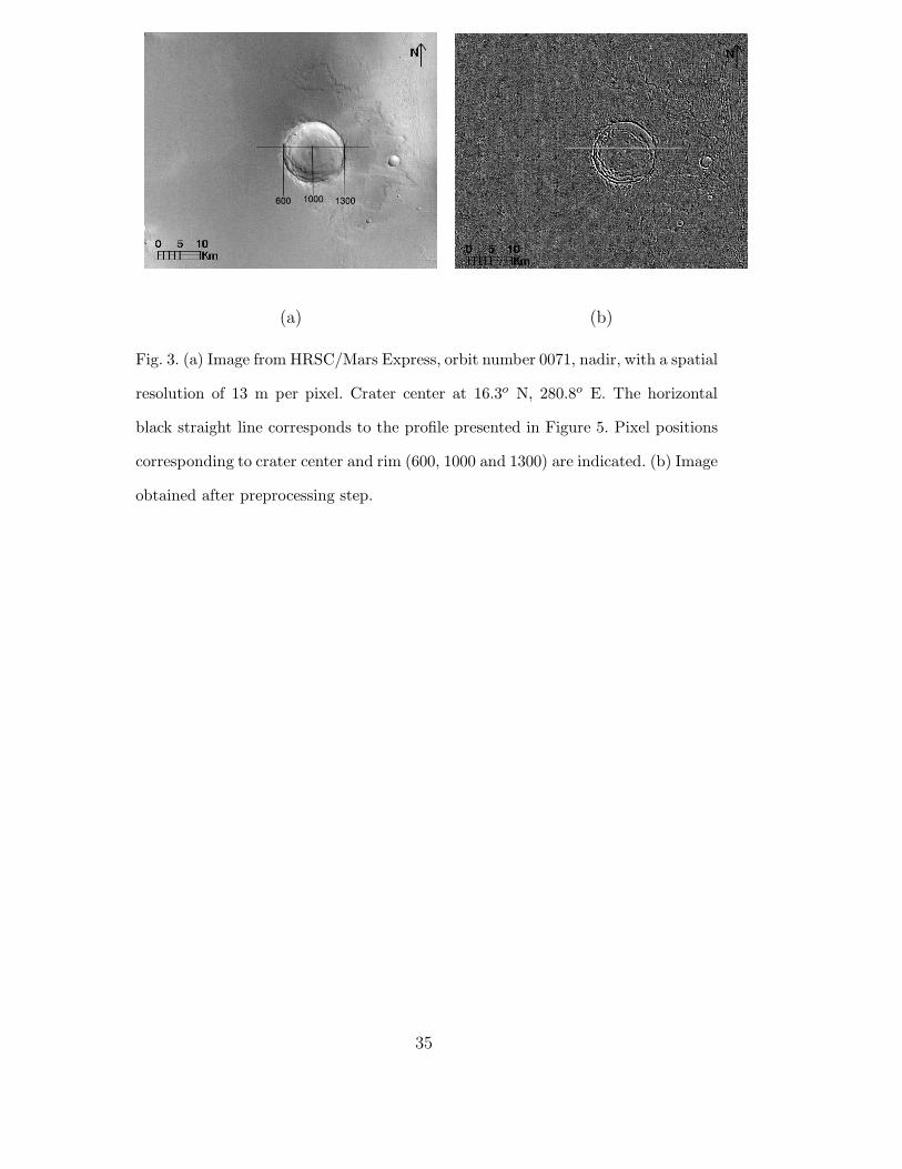
Fig. 3. (a) Image from HRSC/Mars Express, orbit number 0071, nadir, with a spatial

resolution of 13 m per pixel. Crater center at 16.3o N, 280.8o E. The horizontal

black straight line corresponds to the profile presented in Figure 5. Pixel positions

corresponding to crater center and rim (600, 1000 and 1300) are indicated. (b) Image

obtained after preprocessing step.

35

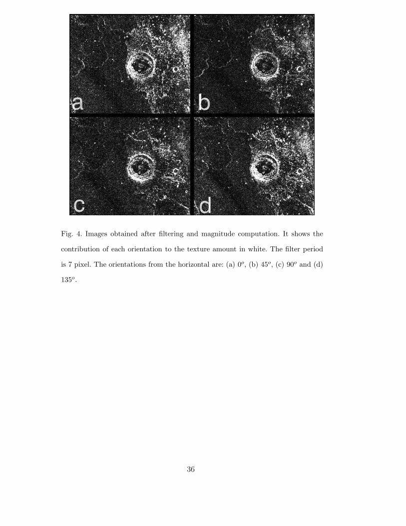
Fig. 4. Images obtained after filtering and magnitude computation. It shows the

contribution of each orientation to the texture amount in white. The filter period

is 7 pixel. The orientations from the horizontal are: (a) 0o, (b) 45o, (c) 90o and (d)

135o.

36

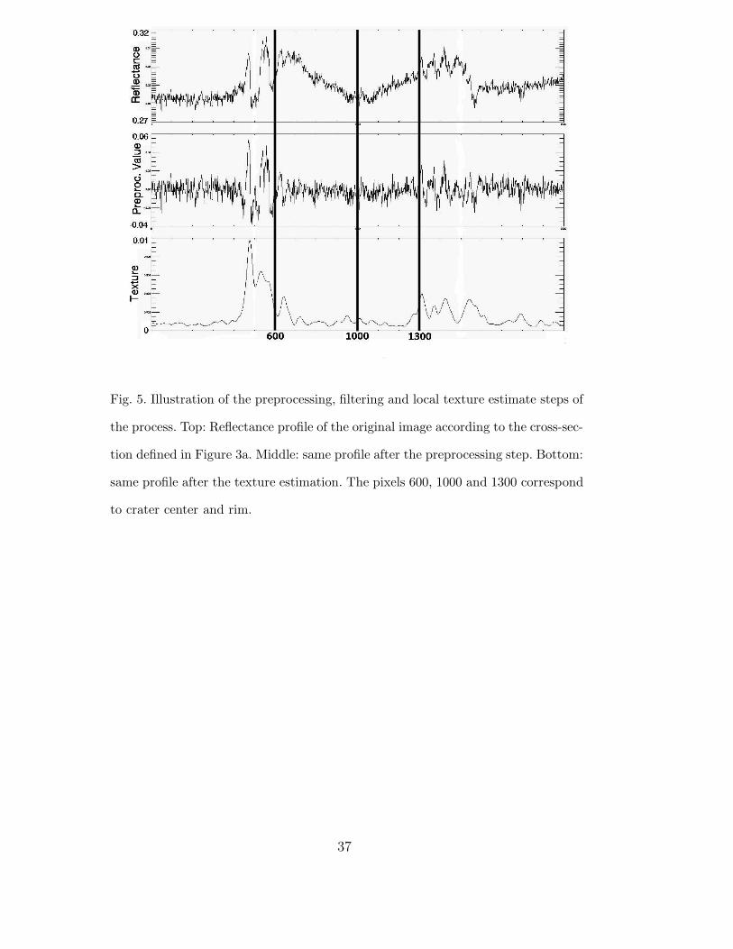
Fig. 5. Illustration of the preprocessing, filtering and local texture estimate steps of

the process. Top: Reflectance profile of the original image according to the cross-sec-

tion defined in Figure 3a. Middle: same profile after the preprocessing step. Bottom:

same profile after the texture estimation. The pixels 600, 1000 and 1300 correspond

to crater center and rim.

37

(a) (b) (c)

Fig. 6. Example of roughness images corresponding to simulated topographic sur-

faces with β values of 3 (a), 5 (b), and 9 (c). The incidence angle is 45o in this

example.

38

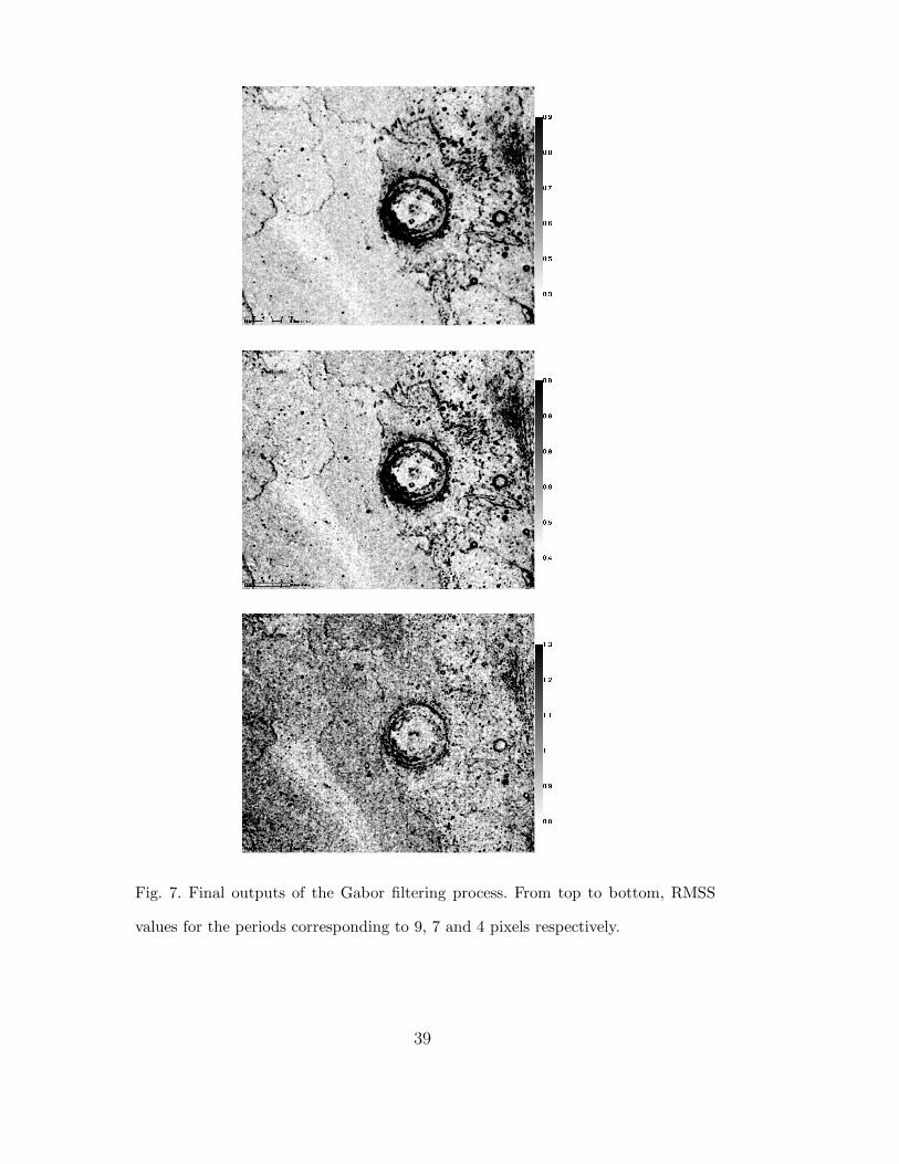
Fig. 7. Final outputs of the Gabor filtering process. From top to bottom, RMSS

values for the periods corresponding to 9, 7 and 4 pixels respectively.

39

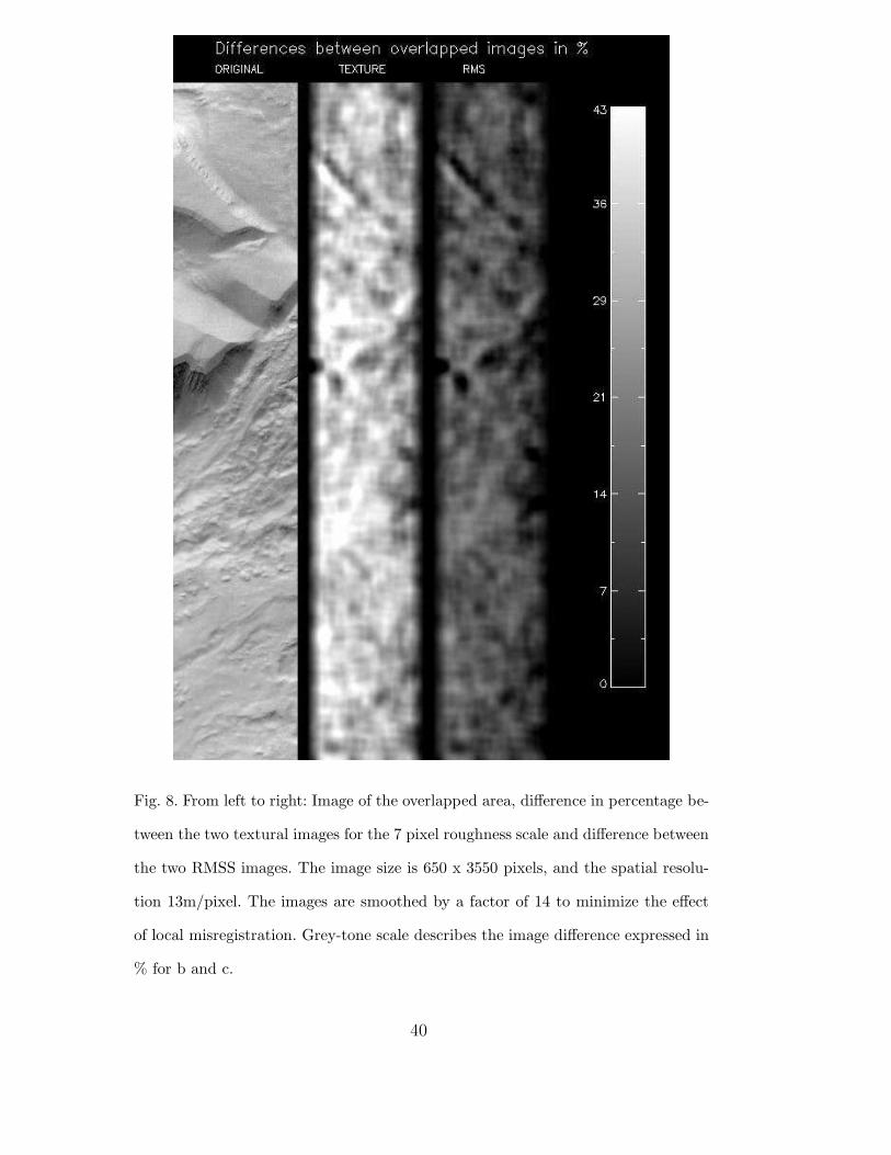
Fig. 8. From left to right: Image of the overlapped area, difference in percentage be-

tween the two textural images for the 7 pixel roughness scale and difference between

the two RMSS images. The image size is 650 x 3550 pixels, and the spatial resolu-

tion 13m/pixel. The images are smoothed by a factor of 14 to minimize the effect

of local misregistration. Grey-tone scale describes the image difference expressed in

% for b and c.

40

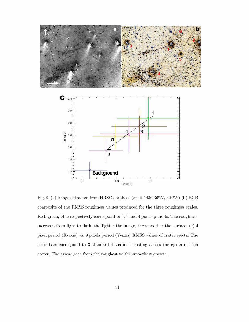
Fig. 9. (a) Image extracted from HRSC database (orbit 1436 36oN , 324oE) (b) RGB

composite of the RMSS roughness values produced for the three roughness scales.

Red, green, blue respectively correspond to 9, 7 and 4 pixels periods. The roughness

increases from light to dark: the lighter the image, the smoother the surface. (c) 4

pixel period (X-axis) vs. 9 pixels period (Y-axis) RMSS values of crater ejecta. The

error bars correspond to 3 standard deviations existing across the ejecta of each

crater. The arrow goes from the roughest to the smoothest craters.

41

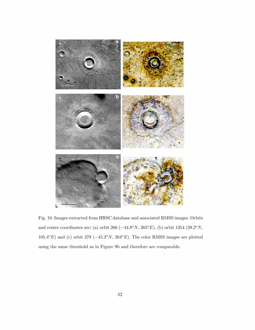
Fig. 10. Images extracted from HRSC database and associated RMSS images. Orbits

and center coordinates are: (a) orbit 266 (−44.8oN , 265oE), (b) orbit 1354 (39.2oN ,

105.4oE) and (c) orbit 279 (−45.2oN , 264oE). The color RMSS images are plotted

using the same threshold as in Figure 9b and therefore are comparable.

42

Fig. 11. Images extracted from HRSC database and associated RMSS images. Orbits

and center coordinates are: (a) orbit 1425 (66.3oN , 323.3oE), (b) orbit 228 (14oN ,

158oE) and (c) orbit 1152 (−13.5oN , 161oE). The color RMSS images are plotted

using the same threshold as in Figure 9b and therefore are comparable.

43

-1200 m - 100 m

(a) (b)

(c)

(d)

Fig. 12. (a) High-resolution (13m/pixel) image of the studied area, from HRSC im-

age h0071 0000. (b) Topography from MOLA data. (c) Simplified geological cross–

section of the studied crater. The vertical exaggeration is 14. (d) RGB composite

of the RMSS roughness values.

44