Surface Reconstruction Based on Lower Dimensional Localized Delaunay Triangulation

EUROGRAPHICS 2000 / M. Gross and F.R.A. Hopgood(Guest Editors)

Volume 19(2000), Number 3

Surface Reconstruction based on Lower DimensionalLocalized Delaunay Triangulation

M. Gopiy S. Krishnan C.T. Silva

AT&T Labs - Research180 Park Avenue

Florham Park, NJ 07932

AbstractWe present a fast, memory efficient algorithm that generates a manifold triangular mesh S passing through a setof unorganized points P� R3. Nothing is assumed about the geometry, topology or presence of boundaries inthe data set except that P is sampled from a real manifold surface. The speed of our algorithm is derived from aprojection-based approach we use to determine the incident faces on a point. We define our sampling criteria tosample the surface and guarantee a topologically correct mesh after surface reconstruction for such a sampledsurface. We also present a new algorithm to find the normal at a vertex, when the surface is sampled accordingour given criteria. We also present results of our surface reconstruction using our algorithm on unorganized pointclouds of various models.

1. Introduction

The problem of surface reconstruction from unorganizedpoint clouds has been, and continues to be, an importanttopic of research. The problem can be loosely stated as fol-lows: Given a set of points P which are sampled from a sur-face inR3, construct a surface S so that the points of P lieon S. A variation of thisinterpolatorydefinition is whenSapproximatesthe set of pointsP.

There are a wide range of applications for which surfacereconstruction is important. For example, scanning complex3D shapes like objects, rooms and landscapes with tactile,optical or ultrasonic sensors are a rich source of data for anumber of analysis and exploratory problems. Surface rep-resentations are a natural choice because of their applica-bility in rendering applications and surface-based visual-izations (like information-coded textures on surfaces). Thechallenge for surface reconstruction algorithms is to findmethods which cover a wide variety of shapes. We brieflydiscuss some of the issues involved in surface reconstruc-tion.

y graduate student at Department of Computer Science, Universityof North Carolina at Chapel Hill, USA

We assume in this paper that the inputs to the surface re-construction algorithm are sampled from an actual surface(or groups of surfaces). A proper reconstruction of thesesurfaces is possible only if they are “sufficiently” sampled.However, sufficiency conditions like sampling theorems arefairly difficult to formulate and as a result, most of the exist-ing reconstruction algorithms ignore this aspect of the prob-lem. Exceptions include the works of3; 5; 2.

If the surface is improperly sampled, the reconstructionalgorithm can produce artifacts. A common artifact is thepresence of spurious surface boundaries in the model. Man-ual intervention or additional information about the sampledsurface (for instance, that the surface is manifold withoutboundaries) are possible ways to eliminate these artifacts.The other extreme in the sampling problem is that the sur-face is sampled unnecessarily dense. This case occurs whena uniformly sampled model with a few fine details can causetoo many data points in areas of low curvature variation.

The choice of underlying mathematical and data structuralrepresentation of the derived surface is also important. Themost common choice are triangular or polygonal mesh rep-resentations. Triangular meshes also allow us to express thetopological properties of the surface, and it is the most popu-

c The Eurographics Association and Blackwell Publishers 2000. Published by BlackwellPublishers, 108 Cowley Road, Oxford OX4 1JF, UK and 350 Main Street, Malden, MA02148, USA.

http://www.eg.org

http://diglib.eg.org

M. Gopi, S. Krishnan, C.T. Silva / Surface Reconstruction

lar model representation for visualization and rendering ap-plications.

Currently, most of the surface reconstruction algorithmsthat guarantee a “good” quality triangulation and are the-oretically sound typically produce higher dimensional sim-plicials like tetrahedra. A second stage of these algorithmsremove interior facets to produce the final triangulation.Therefore, these algorithms usually take on the order of afew minutes to run on data sets of moderate sizes (about20000 to 30000 points) and their applicability to very largedata sets (order of millions of points) is not very clear. In thispaper, we present an algorithm which guarantees a correctreconstruction (and a good quality triangulation) under someassumptions about the underlying object and runs more thanan order of magnitude faster than the above mentioned algo-rithms.

1.1. Main Contributions

In this paper, we present a fast and efficient algorithm forsurface reconstruction from unorganized point clouds basedon localized two-dimensional Delaunay triangulation. Ouralgorithm incrementally develops an interpolatory surfaceusing the surface oriented properties of the given data points.The main contributions of this paper include:

� Sampling criteria: We present a new local sampling cri-teria for the problem of surface reconstruction. The crite-ria is based on directional curvatures on the surface thatis sampled. Based on this criteria and some well placedassumptions about the underlying surface, our algorithmproduces the correct reconstruction.

� Fast surface reconstruction algorithm: Our algorithmis based on theadvancing fronttechniques for surface re-construction. Each iteration of our algorithm advances thereconstructed surface boundary by choosing one point onit and computing all the faces incident on it.

� Normal estimation algorithm: We also present a newand simple algorithm for robust estimation of normals forthe points in an unorganized point set. It is very similar inapproach to the method of Hoppe et. al.16, but we believethat the formulation is different.

� Fast Delaunay neighborhood computation:We havedeveloped a fast and simple algorithm to compute the De-launay neighborhood on a plane around a point, given anangle ordered set of possible candidate Delaunay neigh-bors. This is supported by a fast algorithm for ordering ofa set of points by angle around a reference point.

� System implementation:We have developed a systembased on the above results and have applied it to a numberof models of varying sizes. The empirical performance ofour system is very encouraging and can generate surfacesfrom point clouds of sizes around 100,000 points in fewtens of seconds.

2. Previous Work

The problem of surface reconstruction has received signif-icant attention from researchers in computational geometryand computer graphics. In this section, we give a brief surveyof existing reconstruction algorithms. We use a classificationscheme by Mencl et. al.21 to categorize the various methods.The main classes of reconstruction algorithms are based onspatial subdivision, distance functions, surface warpingandincremental surface growing.

The common theme in spatial subdivision techniques isthat a bounding volume around the input data set is subdi-vided into disjoint cells. The goal of these algorithms is tofind cells related to the shape of the point set. The cell selec-tion scheme can be surface-based or volume-based.

The surface-based scheme proceeds by decomposing thespace into cells, finding the cells that are traversed by the sur-face and finding the surface from the selected cells. The ap-proaches of16; 11; 4; 3 fall under this category. The differencesin their methods lie in the cell selection strategy. Hoppe et.al. 16; 17 use a signed distance function of the surface fromany point to determine the selected cells. Bajaj et. al4 con-struct an approximate surface usingα-solids to determinethe signed distance function. Edelsbrunner and Mucke22; 11

introduce the notion ofα-shapes, a parameterized construc-tion that associates a polyhedral shape with a set of points.The choice ofα has to be determined experimentally. Morerecently, Guo et. al.13 use visibility algorithms and Teich-mann et. al.27 use density scaling and anisotropic shap-ing to improve the results of reconstruction usingα-shapes.For the two-dimensional case, Attali3 introducesnormalizedmeshesto give bounds on the sampling density within whichthe topology of the original curve is preserved.

The volume-based scheme decomposes the space intocells, removes those cells that are not in the volume boundedby the sampled surface and creates the surface from theselected cells. Most algorithms in this category are basedon Delaunay triangulation of the input points. The earli-est of these approaches is Boissonat’s8 “Delaunay sculpt-ing” algorithm that successively removes tetrahedra basedon their circumspheres. Veltkamp29 uses a parameter calledγ-indicator to determine the sequence of tetrahedra to beremoved. The advantage of this algorithm is that theγ-indicator value adapts to variable point density. However,both the approaches of Boissonat and Veltkamp cannot han-dle objects with holes and surface boundaries. Amenta et.al. 2; 1 use a Voronoi filtering approach based on three-dimensional Voronoi diagram and Delaunay triangulation toconstruct thecrust of the sample points. They provide the-oretical guarantees on the topology of their reconstructedmesh given “good” sampling.

The distance function of a surface gives the shortest dis-tance from any point to the surface. The surface passesthrough the zeroes of this distance function. This approachleads to approximating instead of interpolatory surfaces

c The Eurographics Association and Blackwell Publishers 2000.


16; 7; 10. Hoppe et. al.16 use a Reimannian graph to computeconsistent normal throughout the surface to determine thesigned distance function. The approach of Curless and Levoy10 is fine-tuned for laser range data. Their algorithm is wellsuited for handling very large data sets.

Warping-based reconstruction methods deform an initialsurface to give a good approximation of the input point set.This method is particularly suited if a rough approximationof the desired shape is already known. Terzopoulos et. al.28 usedeformable superquadricsto fit the input data points.A different approach to warping was suggested by Szeliskiet. al.25 with oriented particles. By modeling the interactionbetween the particles, they construct the surface using forcesand repulsion.

The basic idea behind incremental surface construction isto build-up the surface using surface-oriented properties ofthe input data points. The approach of Mencl and Muller19; 20 is to start with a global wireframe of the surface gener-ated using Euclidean minimum spanning tree construction,and to fill it iteratively to complete the surface. Boissonnat’ssurface contouring algorithm8 starts with an edge and it-eratively attaches further triangles at boundary edges of theemerging surface using a projection-based approach. Thisalgorithm is similar in vein to our approach. A crucial dif-ference between our methods is that Boissonnat’s algorithmis edge-based, while ours is vertex-based. We also provideguarantees on quality triangulation. Further, his algorithmcan only generate manifolds without boundaries.

The Spiraling-Edge triangulation technique proposed byCrossno and Angel9 is also related to ours. Major differ-ences include the fact that they make several limiting as-sumptions about the data, including normal information foreach point, and also an estimate of each point’s neighbors.Their algorithm works by creating a star-shaped triangula-tion between a point and its neighbors. But the paper pro-vides no theoretical foundation for the actual triangulationcomputed, including no estimates for the sampling neces-sary to produce correct triangulations.

Another recent advancing-front triangulation scheme isthe Ball-Pivoting Algorithm (BPA) of Bernardini et al6.Given a point cloud and a radiusρ, BPA finds an interpola-tory surface where each of its triangles are characterized bythe fact that the ball of radiusρ that sits on its vertices hasno internal point (i.e., it is anρ-exposed triangle). The al-gorithm works by finding a “seed”ρ-exposed triangle, thenextending the surface as far as it can by “pivoting” a ballof radiusρ along each boundary edge of the current sur-face (which is continuously updated). Under some samplingconditions, BPA is guaranteed to finish with a correct tri-angulation. One shortcoming of BPA is the fact that it doesnot allow for reconstructing surfaces out of variable-sampledpoints without multiple passes and they assume that the nor-mal information is available for the input point set.

3. Algorithm Overview

Our surface reconstruction algorithm takes a set of unorga-nized 3D pointsS as input with no other additional infor-mation like normals. The output of the algorithm is a set oftriangles, which defines a manifold surface with or withoutboundary, passing through the input set of points. This algo-rithm uses a progressive triangulation technique where thetriangulation incrementally progresses over the surface. Theneighbors of a vertex in the final triangulation is computedon its tangent plane. Hence it is a local triangulation tech-nique.

Our surface reconstruction algorithm goes through fourmajor steps: normal computation, candidate point selection,Delaunay neighbor computation, and finally the triangula-tion step. This section gives a brief description of all theabove steps.

Normal Computation:The first step in our algorithm is tocompute the normal at all sample points. This step is per-formed only if we the normal information is not part of theinput. This step also consistently orients the normals of thesample points to get an orientable manifold.

Candidate points selection:This step chooses those pointswhich might be possible neighbors to a vertex in the final tri-angulation. Using our sampling criteria described in Section4, we compute this candidate point set (Pp) for every samplepoint p.

Delaunay Neighbor Computation:We map each of thecandidate points in the setPp on the tangent plane atp bya simple rotation about a well defined axis on the tangentplane. The set of these mapped candidate points are referredasPT

p . Then we compute the local Delaunay neighborhoodfrom the setPT

p aroundp in its tangent plane. This compu-tation is repeated for all the points inS, and the final surfacetriangulation is determined from this neighborhood relation-ship.

The candidate point setPp plays a crucial role in deter-mining the final triangulation. In order to obtain the correctsurface, we must impose a certain sampling criteria. In thenext section we formulate this criteria mathematically. Wealso justify the above algorithm using the sampling criteria.

4. Sampling Criteria

In this section, we present a sampling criteria to guarantee atriangulation homeomorphic to the surfaceF. The samplingdensity at a point along a particular direction (in the tangentplane) isinversely proportionalto thedirectional curvatureat that point. The geometric intuition behind this criteria isthat the positioning of the normals of the set of point sam-ples on the Gaussian sphere is uniform provided the productof the directional curvature and the arc length on the sur-face is constant (see24 for an explanation of this fact). In the



p

N

Tc(t)

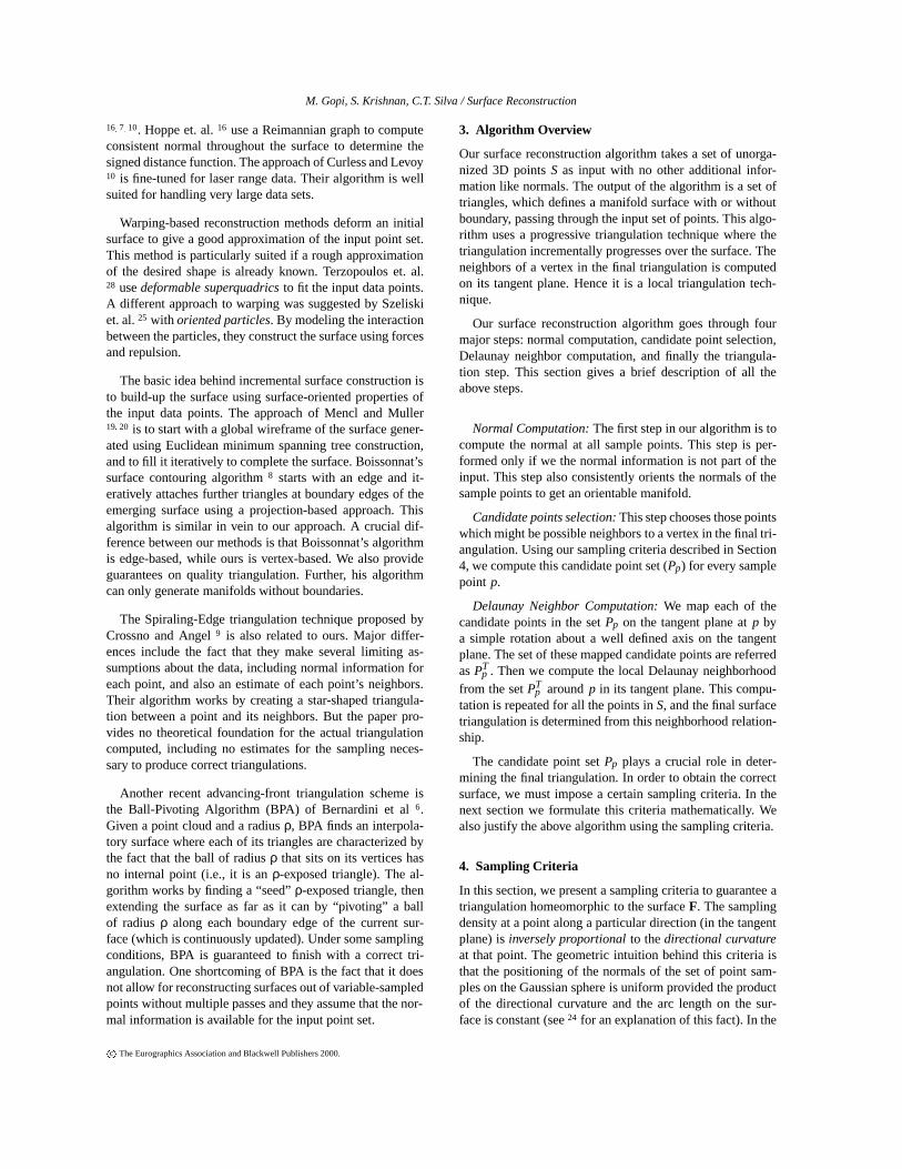
Figure 1: The Darboux Frame

rest of this section, we shall quantitatively explain what theabove criteria means using concepts from differential geom-etry. We shall start by giving a few definitions and notationswhich will be used by us. More detailed explanations can befound in the appendix.

� Consider a pointp on a surfaceF as shown in Figure 1.Let the normal vector toF at p be~N. Given a unit vector~von the tangent plane atp, define a curvec(t) : [�ε;ε]! Fsuch thatc(0) = p, c0(0) = v. TheDarboux frame at p isdefined as the orthonormal differential frame~T =~v;~B=~N�~T;~N. Figure 1 shows the Darboux frame on the sur-face of a cone. It is easy to see that for surfaces with awell defined tangent plane everywhere, every point on thesurface has a unique Darboux frame associated with it ina given direction v in the tangent plane.

� Surface curvature: Associating a local differential frameat every point on the surface allows us to measure somegeometric invariants on the surface. If we walk infinites-imally along a direction~v, the change of the surface nor-mal in the direction~v is called thenormal curvature. Aswe move along different directions in the tangent plane,the normal curvaturevaries. The directions with mini-mum and maximum normal curvatures are called princi-pal directions and the corresponding curvatures in thesedirections are called principle curvatures. These principaldirections are orthogonal to each other. In the rest of thispaper, we will refer to the principal curvatures ask1 andk2 (or kmin andkmax).

� Local surface as a height function:We make use of thewell known implicit function theorem23 to express thesurface in the neighborhood of a point as a height functionin terms of the principal curvatures. We will represent theheight function in the local neighborhood as

h(x;y) =12(k1x2+k2y2)+higher order terms

h(r;θ)� r2

2(k1 cos2 θ+k2sin2θ);

wherer =p

x2+y2 andθ is the angle the vector(x;y)makes with thex-axis. The derivation of the above ex-pression is given in detail in the appendix.

� The Euler equationrelates the normal curvature,kv, atsome pointp on the surface along a direction~v in the tan-gent plane to the principal curvatures,k1 andk2. Let theprincipal directions atp be~v1 and~v2. Then

kv = k1 cos2 θ+k2sin2θ;

whereθ represents the angle~v makes with~v1.Using this result on the expression forh(r;θ) above, weget

h(r;θ) = kvr2

2(1)

� It is possible to describe the behavior of the normal vectoralong space curves on a surfaceF passing through somepoint p. The equation below can be derived from the Car-tan’s equations for differential frames18; 23.

∂~N =�kv∂s~T� t∂s~B;or (2)

j∂~Nj=q

k2v + t2 j∂sj (3)

Here kv is the normal curvature andt (also known asgeodesic torsion) intuitively measures the twist along the~N�~B plane.The quantity

pk2

v + t2 is called thetotal curvatureof thespace curve throughp. We simplify the above equationfor the special case of planar curves throughp for whicht is always zero. Then the total curvature becomeskv, thenormal curvature. Our sampling criterion now can be for-mulated mathematically as

kv∂s= constant (4)

Intuitively, this sampling implies that the dot product be-tween the normals at a given point on the surface and thenearby point samples is constant. Higher the curvature ina particular direction, closer the point samples should beand vice-versa.

� We call a pointp on a surfaceF a regular point if thesurface in the neighborhood ofp is homeomorphic to anopen disk. We replace the constant term in equation 4 byδ and the arc length∂sby the edge length. Given aregularpoint p on F with unit normalNp, let Cδ

p be the (closed)contour onF aroundp such that

kvjpqj = δ;8q2Cδp;v= (~pq� (~pq�Np)Np);

where jpqj denote the Euclidean arc length along the



surface. It is clear thatCδp partitions surfaceF into two

(or more) parts: one that containsp and others that donot. We define the former partition as theimmediateδ-neighborhood(Bδ

p) of the pointp.� We call a point setSa δ-samplingof a surfaceF if every

point p2 F has a closest pointq in the sample setSsuchthatq2Cδ

p. In the above definition,δ is a parameter thatcan be changed to obtain different samples of the surface.

The definition of aδ-sampling is clearly a local samplingcriterion and makes an intrinsic assumption about the tubularneighborhood of the underlying object. This has the disad-vantage of not being sensitive to global features of the objectlike two layers of the same object coming very close to eachother. We make some assumptions on the tubular neighbor-hood of the object. Given a pointq2 F not in theimmediateδ-neighborhoodof p, we place a bound (function ofδ andprincipal curvatures) on the dot product of the vector~pqwiththe unit normal atp. For the rest of this discussion, we willassume that

� The surface under consideration is smooth and that theratio of the maximum to minimum principal curvature atany point is bounded above by the constantρ.

� The arcpqv along the surface can be replaced by the edgepqv. This assumption is reasonable for smallδ.

In this section, we shall state without proof a couple ofproperties aboutδ-sampled surfaces. The proofs are given inthe appendix.

Lemma 1Given aδ-sampleSof a surfaceF and two pointsp;q2 Ssuch thatq2Cδ

p. Thenp2Cδq.

The above lemma will later be used to claim the symme-try in the choice of neighborhood around a point. We nowproceed to show that ratio of the distances between any twopointsq; r 2Cδ

p to p is bounded.

Let p2 F. Define the contourCδp aroundp as before.

Theorem 1(a) Consider any two pointsq; r 2Cδp. Then the

maximum ratio of edge distancesjpqjjprj is bounded above by

a function of principal curvatures.(b) Let Np be the unit normal toF at p and let ˆpq de-note the unit vector fromp to q. Define the height functionH(p;q) = jNp � ~pqj. ThenH(p;q) is bounded above by the

quantityp

1+δ2�1kmin

. kmin is the smaller of the principal curva-tures.(c) Define the angle functionD(p;q) = jNp � p̂qj. Then

D(p;q) is a constant,p

1+δ2�1p1+δ2+1

, for all q2Cδp.

The result about the height function can be used to pre-cisely quantify how close two different parts of the modelcan come so that aδ sampling is sufficient for the recon-struction algorithm. Since the maximum height value for

any point inCδp is bounded by

p1+δ2�1kmin

, we bound the dis-tance between two different layers of the model to be greater

p

q

r

s

Cp

Cq

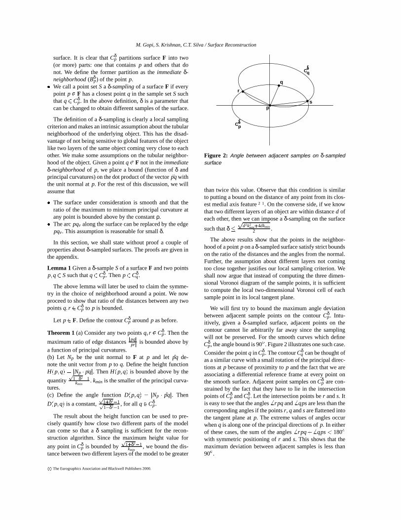
Figure 2: Angle between adjacent samples on δ-sampledsurface

than twice this value. Observe that this condition is similarto putting a bound on the distance of any point from its clos-est medial axis feature2; 1. On the converse side, if we knowthat two different layers of an object are within distanced ofeach other, then we can impose aδ-sampling on the surface

such thatδ�p

d2k2min+4dkmin

2 .

The above results show that the points in the neighbor-hood of a pointpon aδ-sampled surface satisfy strict boundson the ratio of the distances and the angles from the normal.Further, the assumption about different layers not comingtoo close together justifies our local sampling criterion. Weshall now argue that instead of computing the three dimen-sional Voronoi diagram of the sample points, it is sufficientto compute the local two-dimensional Voronoi cell of eachsample point in its local tangent plane.

We will first try to bound the maximum angle deviationbetween adjacent sample points on the contourCδ

p. Intu-itively, given a δ-sampled surface, adjacent points on thecontour cannot lie arbitrarily far away since the samplingwill not be preserved. For the smooth curves which defineCδ

p, the angle bound is 90�. Figure 2 illustrates one such case.

Consider the pointq in Cδp. The contourCδ

q can be thought ofas a similar curve with a small rotation of the principal direc-tions atp because of proximity top and the fact that we areassociating a differential reference frame at every point onthe smooth surface. Adjacent point samples onCδ

p are con-strained by the fact that they have to lie in the intersectionpoints ofCδ

p andCδq. Let the intersection points ber ands. It

is easy to see that the angles6 rpq and6 qpsare less than thecorresponding angles if the pointsr, qandsare flattened intothe tangent plane atp. The extreme values of angles occurwhenq is along one of the principal directions ofp. In eitherof these cases, the sum of the angles6 rpq+ 6 qps< 180�with symmetric positioning ofr ands. This shows that themaximum deviation between adjacent samples is less than90�.



p q

r

s

d

d

0.707d

t

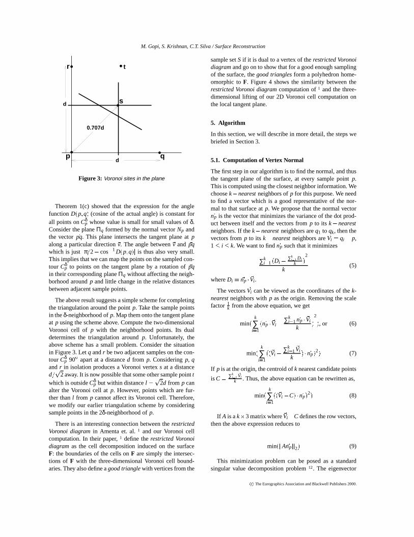
Figure 3: Voronoi sites in the plane

Theorem 1(c) showed that the expression for the anglefunction D(p;q) (cosine of the actual angle) is constant forall points onCδ

p whose value is small for small values ofδ.Consider the planeΠq formed by the normal vectorNp andthe vector~pq. This plane intersects the tangent plane atpalong a particular direction~v. The angle between~v and ~pqwhich is justjπ=2� cos�1 D(p;q)j is thus also very small.This implies that we can map the points on the sampled con-tour Cδ

p to points on the tangent plane by a rotation of~pqin their corresponding planeΠq without affecting the neigh-borhood aroundp and little change in the relative distancesbetween adjacent sample points.

The above result suggests a simple scheme for completingthe triangulation around the pointp. Take the sample pointsin theδ-neighborhood ofp. Map them onto the tangent planeat p using the scheme above. Compute the two-dimensionalVoronoi cell of p with the neighborhood points. Its dualdetermines the triangulation aroundp. Unfortunately, theabove scheme has a small problem. Consider the situationin Figure 3. Letq andr be two adjacent samples on the con-tour Cδ

p 90� apart at a distanced from p. Consideringp, qandr in isolation produces a Voronoi vertexs at a distanced=p

2 away. It is now possible that some other sample pointtwhich is outsideCδ

p but within distancel =p

2d from p canalter the Voronoi cell atp. However, points which are fur-ther thanl from p cannot affect its Voronoi cell. Therefore,we modify our earlier triangulation scheme by consideringsample points in the 2δ-neighborhood ofp.

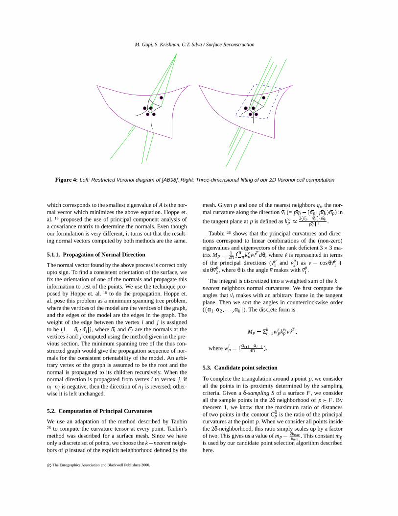
There is an interesting connection between therestrictedVoronoi diagramin Amenta et. al.1 and our Voronoi cellcomputation. In their paper,1 define therestricted Voronoidiagram as the cell decomposition induced on the surfaceF: the boundaries of the cells onF are simply the intersec-tions of F with the three-dimensional Voronoi cell bound-aries. They also define agood trianglewith vertices from the

sample setS if it is dual to a vertex of therestricted Voronoidiagramand go on to show that for a good enough samplingof the surface, thegood trianglesform a polyhedron home-omorphic toF. Figure 4 shows the similarity between therestricted Voronoi diagramcomputation of1 and the three-dimensional lifting of our 2D Voronoi cell computation onthe local tangent plane.

5. Algorithm

In this section, we will describe in more detail, the steps webriefed in Section 3.

5.1. Computation of Vertex Normal

The first step in our algorithm is to find the normal, and thusthe tangent plane of the surface, at every sample pointp.This is computed using the closest neighbor information. Wechoosek�nearestneighbors ofp for this purpose. We needto find a vector which is a good representative of the nor-mal to that surface atp. We propose that the normal vector~np is the vector that minimizes the variance of the dot prod-uct between itself and the vectors fromp to its k�nearestneighbors. If thek�nearestneighbors areq1 to qk, then thevectors fromp to its k�nearestneighbors are~Vi = qi � p,1� i � k. We want to find~np such that it minimizes

∑ki=1 (Di � ∑k

i=1 Di

k )2

k(5)

whereDi = ~np �~Vi .

The vectors~Vi can be viewed as the coordinates of thek-nearestneighbors withp as the origin. Removing the scalefactor 1

k from the above equation, we get

min(k

∑i=1

(~np �~Vi � ∑ki=1 ~np �~Vi

k)

2

), or (6)

min(k

∑i=1

((~Vi � ∑ki=1

~Vi

k) � ~np)

2) (7)

If p is at the origin, the centroid ofk nearest candidate points

isC = ∑ki=1

~Vi

k . Thus, the above equation can be rewritten as,

min(k

∑i=1

((~Vi �C) � ~np)2) (8)

If A is ak�3 matrix where~Vi�C defines the row vectors,then the above expression reduces to

min(kA~npk2) (9)

This minimization problem can be posed as a standardsingular value decomposition problem12. The eigenvector



Figure 4: Left: Restricted Voronoi diagram of [AB98], Right: Three-dimensional lifting of our 2D Voronoi cell computation

which corresponds to the smallest eigenvalue ofA is the nor-mal vector which minimizes the above equation. Hoppe et.al. 16 proposed the use of principal component analysis ofa covariance matrix to determine the normals. Even thoughour formulation is very different, it turns out that the result-ing normal vectors computed by both methods are the same.

5.1.1. Propagation of Normal Direction

The normal vector found by the above process is correct onlyupto sign. To find a consistent orientation of the surface, wefix the orientation of one of the normals and propagate thisinformation to rest of the points. We use the technique pro-posed by Hoppe et. al.16 to do the propagation. Hoppe et.al. pose this problem as a minimum spanning tree problem,where the vertices of the model are the vertices of the graph,and the edges of the model are the edges in the graph. Theweight of the edge between the vertexi and j is assignedto be(1� j~ni � ~nj j), where~ni and~nj are the normals at theverticesi and j computed using the method given in the pre-vious section. The minimum spanning tree of the thus con-structed graph would give the propagation sequence of nor-mals for the consistent orientability of the model. An arbi-trary vertex of the graph is assumed to be the root and thenormal is propagated to its children recursively. When thenormal direction is propagated from vertexi to vertex j , ifni �nj is negative, then the direction ofnj is reversed; other-wise it is left unchanged.

5.2. Computation of Principal Curvatures

We use an adaptation of the method described by Taubin26 to compute the curvature tensor at every point. Taubin’smethod was described for a surface mesh. Since we haveonly a discrete set of points, we choose thek�nearestneigh-bors ofp instead of the explicit neighborhood defined by the

mesh. Givenp and one of the nearest neighborsqi , the nor-mal curvature along the direction~vi (= ~pqi � (~np � ~pqi)~np) in

the tangent plane atp is defined askvip � 2(~np� ~nqi )� ~pqi

k ~pqik2 .

Taubin 26 shows that the principal curvatures and direc-tions correspond to linear combinations of the (non-zero)eigenvalues and eigenvectors of the rank deficient 3�3 ma-trix Mp = 1

2πR π�π kv

p~v~vTdθ, where~v is represented in terms

of the principal directions (~vp1 and~vp

2) as~v = cosθ~vp1 +

sinθ~vp2, whereθ is the angle~v makes with~vp

1.

The integral is discretized into a weighted sum of thek�nearestneighbors normal curvatures. We first compute theangles that~vi makes with an arbitrary frame in the tangentplane. Then we sort the angles in counterclockwise order(fα1;α2; : : : ;αkg). The discrete form is

Mp = Σki=1wi

pkvip~v~v

T ;

wherewip = (

αi+1�αi�14π ).

5.3. Candidate point selection

To complete the triangulation around a pointp, we considerall the points in its proximity determined by the samplingcriteria. Given aδ-sampling Sof a surfaceF, we considerall the sample points in the 2δ neighborhood ofp2 F. Bytheorem 1, we know that the maximum ratio of distancesof two points in the contourCδ

p is the ratio of the principalcurvatures at the pointp. When we consider all points insidethe 2δ-neighborhood, this ratio simply scales up by a factorof two. This gives us a value ofmp =

2kmaxkmin

. This constantmp

is used by our candidate point selection algorithm describedhere.



This step is similar to clustering algorithms used by othertriangulation schemes16; 14. We first apply adistance crite-rion to prune down our search for candidate adjacent pointsin the spatial proximity ofp. It is executed in two stages.In the first stage, the simplerL1 metric is used to definethe proximity aroundp. Our algorithm takes an axis-alignedbox of appropriate dimensions centered atp and returns allthe data points inside it. The second stage of pruning usesa Euclidean metric, which further rejects the points that lieoutside asphere of influencecentered atp. Our data structurefor this stage of pruning is a depth pixel array similar to thedexelstructure proposed in15. We maintain a 2D pixel arrayinto which all data points are orthographically projected. Thepoints mapped on to the same pixel are sorted by their depth(z) values. This data structure makes the search for candidatepoints very easy.

By using this data structure, this search is limited to thepixels around the pixel wherep is projected. The size of thebounding box for choosing the candidate points usingL1metric, and the radius of thesphere of influenceused in thesecond stage of pruning is determined by the valuemp. As-suming that the distance ofp from its closest neighbor iss,the bounding box and the sphere should enclose all points,which are at the distance less thanmps from p.

The set of points obtained by these two pruning stagesis further pruned by computing the height values of thesepoints inp’s local tangent plane. If the height value is greater

thanp

1+4δ2�1kmin

(refer to Theorem 1b), we remove thosepoints from consideration because they lie outside the tubu-lar neighborhood of the surface nearp. The points that re-main are the possible Delaunay neighbors ofp.

5.4. Triangulation

The next step is the find the neighbors of each vertex to findthe final triangulation of the surface. Once we have a consis-tent orientation of the normals for all the vertices, we mapthe candidate points as found in Section 5.3 onto the tangentplane at the reference pointp. This mapping is the rotationof the vectorVi , from p to the candidate point, on the planedefined by the normal andVi , to the tangent plane atp. Theseprojected candidate points on the tangent plane are orderedby angle aroundp.

5.4.1. Fast Ordering by Angle

The candidate points are transformed to the local coordinatesystem and are mapped as explained above to the tangentplane atp. These points have 2D coordinates, with an im-plicit definition of coordinate axes. The projected candidatepoint set is partitioned on the basis of the quadrant where thepoints lie on this tangent plane in the local coordinate sys-tem. The points within each quadrant are ordered by angleusing a simple method as explained below.

The square of the sine of the angle from the implicitx�

p

B

Voronoi Edges

CA

M

CL

IBL

BL B

ACI

AL

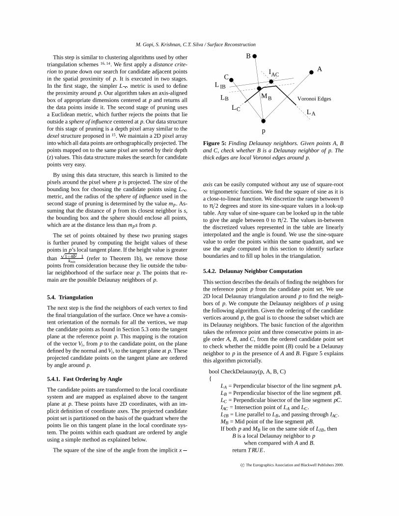
Figure 5: Finding Delaunay neighbors. Given points A, Band C, check whether B is a Delaunay neighbor of p. Thethick edges are local Voronoi edges around p.

axiscan be easily computed without any use of square-rootor trignometric functions. We find the square of sine as it isa close-to-linear function. We discretize the range between 0to π=2 degrees and store its sine-square values in a look-uptable. Any value of sine-square can be looked up in the tableto give the angle between 0 toπ=2. The values in-betweenthe discretized values represented in the table are linearlyinterpolated and the angle is found. We use the sine-squarevalue to order the points within the same quadrant, and weuse the angle computed in this section to identify surfaceboundaries and to fill up holes in the triangulation.

5.4.2. Delaunay Neighbor Computation

This section describes the details of finding the neighbors forthe reference pointp from the candidate point set. We use2D local Delaunay triangulation aroundp to find the neigh-bors of p. We compute the Delaunay neighbors ofp usingthe following algorithm. Given the ordering of the candidatevertices aroundp, the goal is to choose the subset which areits Delaunay neighbors. The basic function of the algorithmtakes the reference point and three consecutive points in an-gle orderA, B, andC, from the ordered candidate point setto check whether the middle point (B) could be a Delaunayneighbor top in the presence ofA andB. Figure 5 explainsthis algorithm pictorially.

bool CheckDelaunay(p, A, B, C){

LA = Perpendicular bisector of the line segmentpA.LB = Perpendicular bisector of the line segmentpB.LC = Perpendicular bisector of the line segmentpC.IAC = Intersection point ofLA andLC.LIB = Line parallel toLB, and passing throughIAC.MB = Mid point of the line segmentpB.If both p andMB lie on the same side ofLIB, then

B is a local Delaunay neighbor topwhen compared withA andB.

returnTRUE.



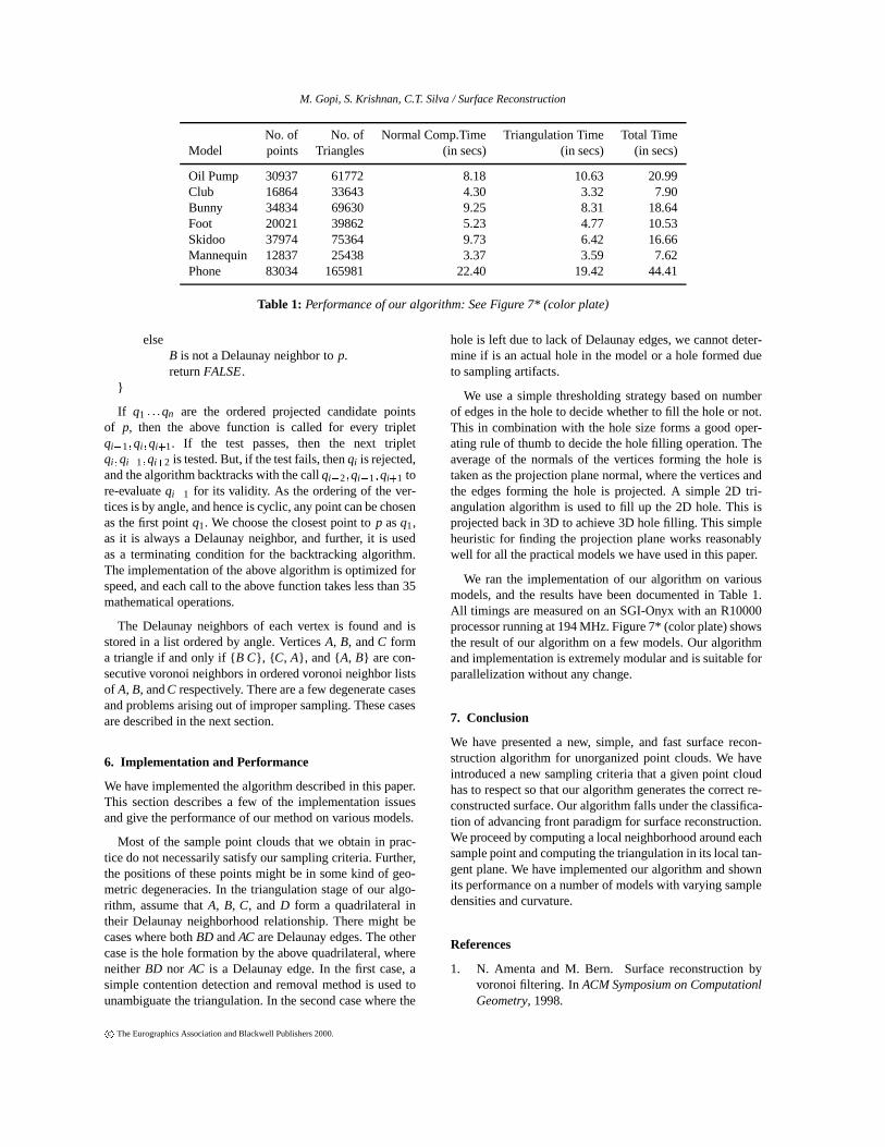
No. of No. of Normal Comp.Time Triangulation Time Total TimeModel points Triangles (in secs) (in secs) (in secs)

Oil Pump 30937 61772 8.18 10.63 20.99Club 16864 33643 4.30 3.32 7.90Bunny 34834 69630 9.25 8.31 18.64Foot 20021 39862 5.23 4.77 10.53Skidoo 37974 75364 9.73 6.42 16.66Mannequin 12837 25438 3.37 3.59 7.62Phone 83034 165981 22.40 19.42 44.41

Table 1: Performance of our algorithm: See Figure 7* (color plate)

elseB is not a Delaunay neighbor top.returnFALSE.

}

If q1 : : :qn are the ordered projected candidate pointsof p, then the above function is called for every tripletqi�1;qi ;qi+1. If the test passes, then the next tripletqi ;qi+1;qi+2 is tested. But, if the test fails, thenqi is rejected,and the algorithm backtracks with the callqi�2;qi�1;qi+1 tore-evaluateqi�1 for its validity. As the ordering of the ver-tices is by angle, and hence is cyclic, any point can be chosenas the first pointq1. We choose the closest point top asq1,as it is always a Delaunay neighbor, and further, it is usedas a terminating condition for the backtracking algorithm.The implementation of the above algorithm is optimized forspeed, and each call to the above function takes less than 35mathematical operations.

The Delaunay neighbors of each vertex is found and isstored in a list ordered by angle. VerticesA, B, andC forma triangle if and only if {B C}, { C, A}, and {A, B} are con-secutive voronoi neighbors in ordered voronoi neighbor listsof A, B, andC respectively. There are a few degenerate casesand problems arising out of improper sampling. These casesare described in the next section.

6. Implementation and Performance

We have implemented the algorithm described in this paper.This section describes a few of the implementation issuesand give the performance of our method on various models.

Most of the sample point clouds that we obtain in prac-tice do not necessarily satisfy our sampling criteria. Further,the positions of these points might be in some kind of geo-metric degeneracies. In the triangulation stage of our algo-rithm, assume thatA, B, C, andD form a quadrilateral intheir Delaunay neighborhood relationship. There might becases where bothBD andAC are Delaunay edges. The othercase is the hole formation by the above quadrilateral, whereneitherBD nor AC is a Delaunay edge. In the first case, asimple contention detection and removal method is used tounambiguate the triangulation. In the second case where the

hole is left due to lack of Delaunay edges, we cannot deter-mine if is an actual hole in the model or a hole formed dueto sampling artifacts.

We use a simple thresholding strategy based on numberof edges in the hole to decide whether to fill the hole or not.This in combination with the hole size forms a good oper-ating rule of thumb to decide the hole filling operation. Theaverage of the normals of the vertices forming the hole istaken as the projection plane normal, where the vertices andthe edges forming the hole is projected. A simple 2D tri-angulation algorithm is used to fill up the 2D hole. This isprojected back in 3D to achieve 3D hole filling. This simpleheuristic for finding the projection plane works reasonablywell for all the practical models we have used in this paper.

We ran the implementation of our algorithm on variousmodels, and the results have been documented in Table 1.All timings are measured on an SGI-Onyx with an R10000processor running at 194 MHz. Figure 7* (color plate) showsthe result of our algorithm on a few models. Our algorithmand implementation is extremely modular and is suitable forparallelization without any change.

7. Conclusion

We have presented a new, simple, and fast surface recon-struction algorithm for unorganized point clouds. We haveintroduced a new sampling criteria that a given point cloudhas to respect so that our algorithm generates the correct re-constructed surface. Our algorithm falls under the classifica-tion of advancing front paradigm for surface reconstruction.We proceed by computing a local neighborhood around eachsample point and computing the triangulation in its local tan-gent plane. We have implemented our algorithm and shownits performance on a number of models with varying sampledensities and curvature.

References

1. N. Amenta and M. Bern. Surface reconstruction byvoronoi filtering. InACM Symposium on ComputationlGeometry, 1998.



2. N. Amenta, M. Bern, and M. Kamvysselis. A newvoronoi-based surface reconstruction algorithm. InProceedings of ACM Siggraph, pages 415–421, 1998.

3. D. Attali. r-regular shape reconstruction from unorga-nized points. InACM Symposium on Computationl Ge-ometry, pages 248–253, 1997.

4. C. Bajaj, F. Bernardini, and G. Xu. Automatic recon-struction of surfaces and scalar fields from 3d scans. InProceedings of ACM Siggraph, pages 109–118, 1995.

5. F. Bernardini and C. Bajaj. Sampling and recon-structing manifolds using alpha-shapes. InProc. ofNinth Canadian Conference on Computational Geom-etry, pages 193–198, 1997.

6. F. Bernardini, J. Mittleman, H. Rushmeier, C. Silva, andG. Taubin. The ball-pivoting algorithm for surface re-construction. IEEE Transactions on Visualization andComputer Graphics, 1999.

7. E. Bittar, N. Tsingos, and M. P. Gascuel. Automatic re-construction from unstructured data: Combining a me-dial axis and implicit surfaces.Computer GraphicsForum, Proceedings of Eurographics, 14(3):457–468,1995.

8. J. D. Boissonnat. Geometric structures for three-dimensional shape representation.ACM Transactionson Graphics, 3(4):266–286, 1984.

9. P. Crossno and E. Angel. Spiraling edge: Fast surfacereconstruction from partially organized sample points.IEEE Visualization ’99, pages 317–324, October 1999.

10. B. Curless and M. Levoy. A volumetric method forbuilding complex models from range images. InPro-ceedings of ACM Siggraph, pages 303–312, 1996.

11. H. Edelsbrunner and E. Mucke. Three dimensional al-pha shapes.ACM Transactions on Graphics, 13(1):43–72, 1994.

12. G.H. Golub and C.F. Van Loan.Matrix Computations.John Hopkins Press, Baltimore, 1989.

13. B. Guo, J. Menon, and B. Willette. Surface reconstruc-tion from alpha shapes.Computer Graphics Forum,16(4):177–190, 1997.

14. B. Heckel, A. C. Uva, and B. Hamann. Clustering-based generation of hierarchical surface models. InC. M. Wittenbrink and A. Varshney, editors,IEEE Vi-sualization ’98: Late Breaking Hot Topics Proceedings,pages 41–44, 1998.

15. T. Van Hook. Real-time shaded NC milling display. InProceedings of ACM Siggraph, pages 15–20, 1986.

16. H. Hoppe, T. Derose, T. Duchamp, J. McDonald, andW. Stuetzle. Surface reconstruction from unorganizedpoint clouds. InProceedings of ACM Siggraph, pages71–78, 1992.

17. H. Hoppe, T. Derose, T. Duchamp, J. McDonald, andW. Stuetzle. Mesh optimization. InProceedings ofACM Siggraph, pages 21–26, 1993.

18. J. Koenderink.Solid Shape. MIT Press, 1989.

19. R. Mencl. A graph-based approach to surface recon-struction. Computer Graphics Forum, Proceedings ofEurographics, 14(3):445–456, 1995.

20. R. Mencl and H. Muller. Graph-based surface recon-struction using structures in scattered point sets.Pro-ceedings of CGI ’98, 1998.

21. R. Mencl and H. Muller. Interpolation and approxima-tion of surfaces from three-dimensional scattered datapoints. State of the Art Reports, Eurographics ’98,pages 51–67, 1998.

22. E. P. Mucke. Shapes and Implementations in Three-Dimensional Geometry. PhD thesis, Department ofComputer Science, University of Illinois at Urbana-Champaign, 1993.

23. B. O’Neill. Elementary Differential Geometry. Aca-demic Press, London, UK, 1966.

24. C. Silva and G. Taubin. Curvature-based estimation ofsurface sampling. InSIAM Conference on GeometricDesign, 1999.

25. R. Szeliski and D. Tonnesen. Surface modeling withoriented particle systems. InProceedings of ACM Sig-graph, pages 185–194, 1992.

26. G. Taubin. Estimating the tensor of curvature of asurface from a polyhedral approximation. InProc. ofICCV, pages 902–907, 1995.

27. M. Teichmann and M. Capps. Surface reconstructionwith anisotropic density-scaled alpha shapes. InPro-ceedings of IEEE Visualization, pages 67–72, 1998.

28. D. Terzopoulos, A. Witkin, and M. Kass. Constraintson deformable models: Recovering 3d shape and non-rigid motion. Artificial Intelligence, 36:91–123, 1988.

29. R. C. Veltkamp. Boundaries through scattered pointsof unknown density.Graphical Models and Image Pro-cessing, 57(6):441–452, 1995.



p=(0,0,0)

xy−plane

M

Wp

Vp

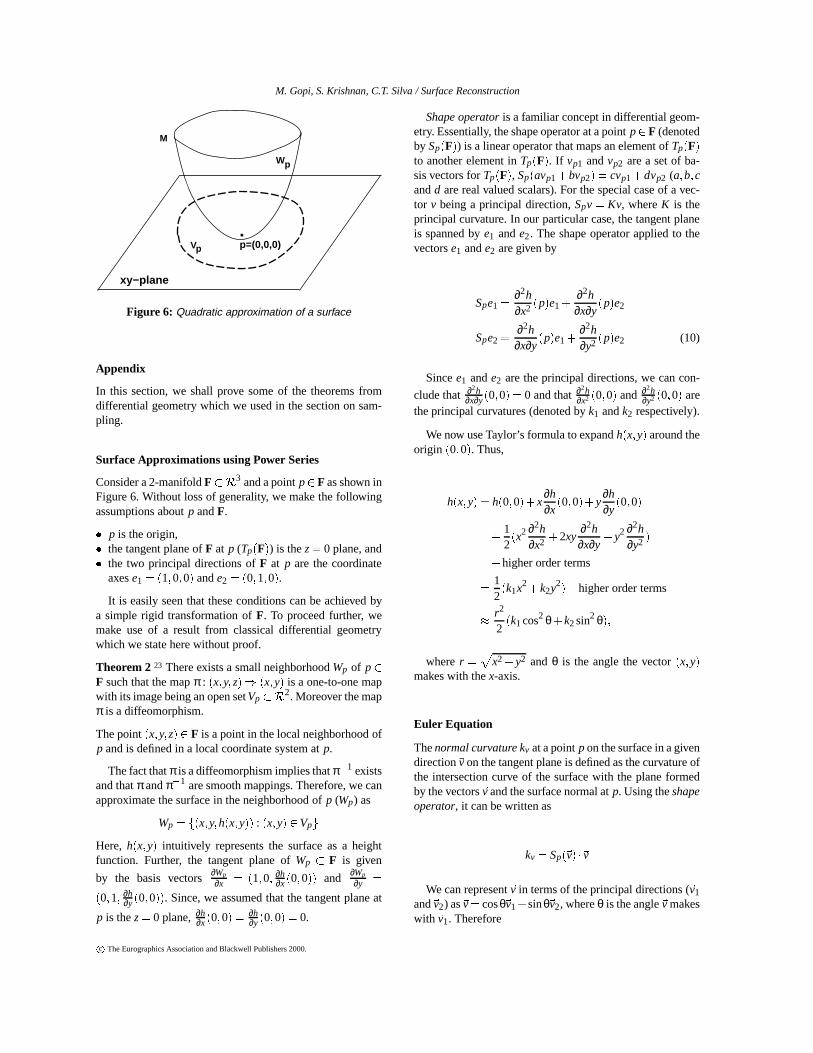
Figure 6: Quadratic approximation of a surface

Appendix

In this section, we shall prove some of the theorems fromdifferential geometry which we used in the section on sam-pling.

Surface Approximations using Power Series

Consider a 2-manifoldF�R3 and a pointp2 F as shown inFigure 6. Without loss of generality, we make the followingassumptions aboutp andF.

� p is the origin,� the tangent plane ofF at p (Tp(F)) is thez= 0 plane, and� the two principal directions ofF at p are the coordinate

axese1 = (1;0;0) ande2 = (0;1;0).

It is easily seen that these conditions can be achieved bya simple rigid transformation ofF. To proceed further, wemake use of a result from classical differential geometrywhich we state here without proof.

Theorem 223 There exists a small neighborhoodWp of p2F such that the mapπ : (x;y;z)) (x;y) is a one-to-one mapwith its image being an open setVp�R2. Moreover the mapπ is a diffeomorphism.

The point(x;y;z)2 F is a point in the local neighborhood ofp and is defined in a local coordinate system atp.

The fact thatπ is a diffeomorphism implies thatπ�1 existsand thatπ andπ�1 are smooth mappings. Therefore, we canapproximate the surface in the neighborhood ofp (Wp) as

Wp = f(x;y;h(x;y)) : (x;y) 2VpgHere, h(x;y) intuitively represents the surface as a heightfunction. Further, the tangent plane ofWp � F is given

by the basis vectors∂Wp

∂x = (1;0; ∂h∂x(0;0)) and ∂Wp

∂y =

(0;1; ∂h∂y(0;0)). Since, we assumed that the tangent plane at

p is thez= 0 plane,∂h∂x(0;0) =

∂h∂y(0;0) = 0.

Shape operatoris a familiar concept in differential geom-etry. Essentially, the shape operator at a pointp2 F (denotedby Sp(F)) is a linear operator that maps an element ofTp(F)to another element inTp(F). If vp1 andvp2 are a set of ba-sis vectors forTp(F), Sp(avp1+bvp2) = cvp1+dvp2 (a;b;candd are real valued scalars). For the special case of a vec-tor v being a principal direction,Spv = Kv, whereK is theprincipal curvature. In our particular case, the tangent planeis spanned bye1 ande2. The shape operator applied to thevectorse1 ande2 are given by

Spe1 =∂2h∂x2 (p)e1+

∂2h∂x∂y

(p)e2

Spe2 =∂2h∂x∂y

(p)e1+∂2h∂y2 (p)e2 (10)

Sincee1 ande2 are the principal directions, we can con-

clude that ∂2h∂x∂y(0;0) = 0 and that∂

2h∂x2 (0;0) and ∂2h

∂y2 (0;0) arethe principal curvatures (denoted byk1 andk2 respectively).

We now use Taylor’s formula to expandh(x;y) around theorigin (0;0). Thus,

h(x;y) = h(0;0)+x∂h∂x

(0;0)+y∂h∂y

(0;0)

+12(x2 ∂2h

∂x2 +2xy∂2h∂x∂y

+y2 ∂2h∂y2 )

+higher order terms

=12(k1x2+k2y2)+higher order terms

� r2

2(k1cos2 θ+k2sin2 θ);

wherer =p

x2+y2 andθ is the angle the vector(x;y)makes with thex-axis.

Euler Equation

Thenormal curvature kv at a pointpon the surface in a givendirection~v on the tangent plane is defined as the curvature ofthe intersection curve of the surface with the plane formedby the vectors~v and the surface normal atp. Using theshapeoperator, it can be written as

kv = Sp(~v) �~v

We can represent~v in terms of the principal directions (~v1and~v2) as~v= cosθ~v1+sinθ~v2, whereθ is the angle~v makeswith~v1. Therefore



kv = Sp(cosθ~v1+sinθ~v2) � (cosθ~v1+sinθ~v2)

= (k1 cosθ~v1+k2 sinθ~v2) � (cosθ~v1+sinθ~v2)

= k1 cos2θ+k2 sin2 θ

The above equation is also known as theEuler equation.It expresses the normal curvature at a point on the surface interms of the principal curvatures there.

Frenet-Serret equations for Darboux Frame

We will now present the equations which govern the behav-ior of the Darboux frame for space curves on a surfaceFpassing throughp. These equations are a modified form ofthe well-known Frenet-Serret equations18; 23.

0B@

∂~T∂s∂~B∂s∂~N∂s

1CA =

0@

0 g kv

�g 0 t�kv �t 0

1A0@

~T~B~N

1A

The entries in the above matrix define the geometrical in-variants at the point in consideration.kv is the componentof the acceleration along the surface normal (normal cur-vature). g (or geodesic curvature) is the component of theacceleration in the tangent plane.t (also known asgeodesictorsion) intuitively measures the twist along the~N�~B plane.

Of this, the third equation governing the change in normalis of most interest to us.

∂~N =�kv∂s~T� t∂s~B;or

j∂~Nj=q

k2v + t2j∂sj

Proofs of various theorems

We shall prove some of the theorems claimed in section 4.

Lemma 1Given aδ-sampleSof a surfaceF and two pointsp;q2 Ssuch thatq2Cδ

p. Thenp2Cδq.

Proof: We will first show that the angle between the normalat p and the normals at all the points onCδ

p is a constant, andis related toδ. Specializing equation (2) by zeroing out thetorsion factor, we know that

~N+ ~∂N = ~N�kv∂s~T (11)

Therefore the cosine of the angle between~N and~N+ ~∂Nis simply 1=

p1+(kv∂s)2 or 1=

p1+δ2 which is a contant.

Since the dot product is just a function ofδ which isconstant throughout the surface, and since the deviation (or

dot product) is symmetric,p2Cδq.

Let p2 F. Define the contourCδp aroundp as before.

Theorem 1 (a) Consider any two pointsq; r 2Cδp. Then the

maximum ratio of edge distancesjpqjjprj is bounded above by

a function of principal curvatures.

(b) Let Np be the unit normal toF at p and let ˆpq de-note the unit vector fromp to q. Define the height functionH(p;q) = jNp � ~pqj. ThenH(p;q) is bounded above by the

quantityp

1+δ2�1kmin

. kmin is the smaller of the principal curva-tures.

(c) Define the angle functionD(p;q) = jNp � p̂qj. Then

D(p;q) is a constant,p

1+δ2�1p1+δ2+1

, for all q2Cδp.

Proof: (a) From equation (4),kvqjpqj = kvr jprj = δ. There-

fore, jpqjjprj =

kvrkvq

. This ratio reaches maximum whenkvr is

maximum andkvq is minimum. They are attained when thetwo directionsvr andvq are the principal directionsv1 andv2. Therefore, the maximum ratio at every point is the ratioof the principal curvatures at that point. But this is boundedby our assumption.

(b) In order to prove the height function bound, letus assume without loss of generality thatp is the ori-gin and the normal vector atp is (0;0;1) and q is givenby the point(x;y;h(x;y)). Then H(p;q) is simply h(x;y).From equation (1) we know thath(x;y) can be rewritten

as kvr2

2 . Also ourδ-sampling criterion gives us the equation

kv

qr2+

k2vr4

4 = δ. After some simple algebraic manipula-

tion and replacingkvr2

2 by h, we get the quadratic equationk2

vh2+2kvh�δ2 = 0. The positive solution of this equation

isp

1+δ2�1kv

. It reaches a maximum when the normal curva-ture is minimum. This value is attained at the smaller of thetwo principal curvatures.

(c) The angle functionD(p;q) = h(x;y)px2+y2+h2(x;y)

. From

equation (1) and simplifying after substitutingr =p

x2+y2,

we getD2(p;q) = k2vr2

(4+k2vr2)

. Using a similar manipulation as

was done for proving the height function bound but substitut-ing k2

vr2 by d, we get the quadratic equationd2+4d�4δ2 =0. The positive root of this quadratic equation is the constant2(p

1+δ2�1). Plugging this value into the expression for

D(p;q), we getp

1+δ2�1p1+δ2+1

. Therefore, all the points in the

curveCδp make the same angle with the normal atp.



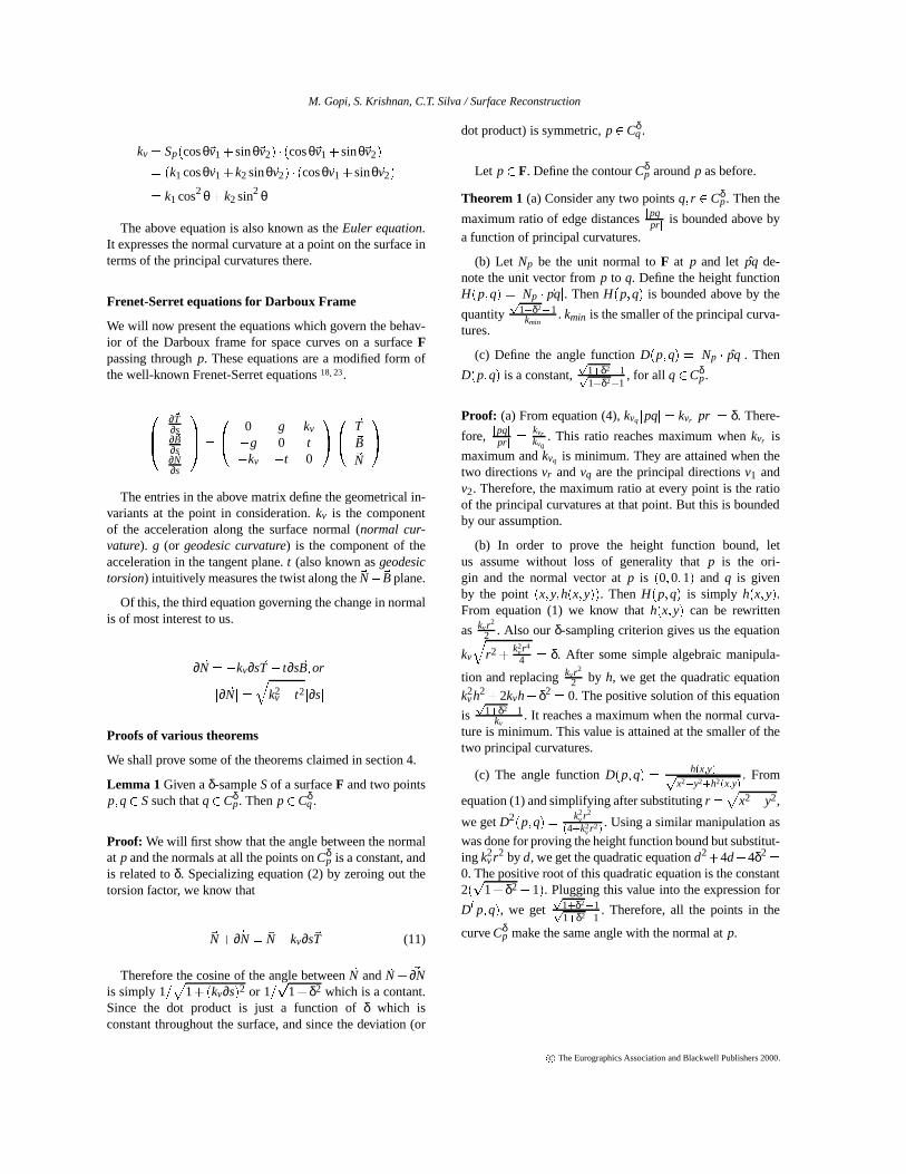
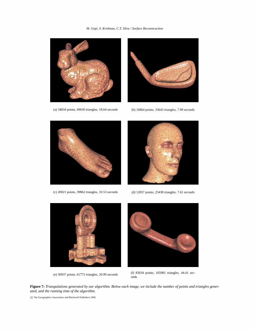
(a) 34834 points, 69630 triangles, 18.64 seconds (b) 16864 points, 33643 triangles, 7.90 seconds

(c) 20021 points, 39862 triangles, 10.53 seconds (d) 12837 points, 25438 triangles, 7.61 seconds

(e) 30937 points, 61772 triangles, 20.99 seconds (f) 83034 points, 165981 triangles, 44.41 sec-onds

Figure 7: Triangulations generated by our algorithm. Below each image, we include the number of points and triangles gener-ated, and the running time of the algorithm.


Surface Reconstruction Based on Lower Dimensional Localized Delaunay Triangulation

Documents