Surface plasmon hybridization and exciton coupling

This is the author’s version of a work that was submitted/accepted for pub-lication in the following source:

Gómez, Daniel E., Roberts, Ann, Davis, Timothy J., & Vernon, Kristy C.(2012) Surface plasmon hybridization and exciton coupling. Physical Re-view B - Condensed Matter and Materials Physics, 86(3), 035411-1.

This file was downloaded from: http://eprints.qut.edu.au/52691/

c© Copyright 2012 American Physical Society

(4) The right to post and update the Article on free-access e-print serversas long as files prepared and/or formatted by APS or its vendors are notused for that purpose. Any such posting made or updated after acceptanceof the Article for publication shall include a link to the online abstract in theAPS journal or to the entry page of the journal. If the author wishes theAPS-prepared version to be used for an online posting other than on theauthor(s)’ or employer’s website, APS permission is required; if permissionis granted, APS will provide the Article as it was published in the journal,and use will be subject to APS terms and conditions.

Notice: Changes introduced as a result of publishing processes such ascopy-editing and formatting may not be reflected in this document. For adefinitive version of this work, please refer to the published source:

http://dx.doi.org/10.1103/PhysRevB.86.035411

Surface Plasmon hybridization and exciton coupling

Daniel E. Gomez,1, 2, ∗ Ann Roberts,1 Timothy J. Davis,2 and Kristy C. Vernon3

1School of Physics, The University of Melbourne, Parkville, VIC, 3010, Australia.2CSIRO, Materials Science and Engineering, Private Bag 33, Clayton, Victoria, 3168, Australia.

3School of Physics, Queensland University of Technology,GPO Box 2434, Brisbane, QLD, 4001, Australia

We derive a semi–analytical model to describe the interaction of a single photon emitter anda collection of arbitrarily shaped metal nanoparticles. The theory treats the metal nanoparticlesclassically within the electrostatic eigenmode method, wherein the surface plasmon resonances ofcollections of nanoparticles are represented by the hybridization of the plasmon modes of the non–interacting particles. The single photon emitter is represented by a quantum mechanical two–levelsystem that exhibits line broadening due to a finite spontaneous decay rate. Plasmon–emittercoupling is described by solving the resulting Bloch equations. We illustrate the theory by studyingmodel systems consisting of a single emitter coupled to one, two and three nanoparticles and wealso compared the predictions of our model to published experimental data.

Keywords:

I. INTRODUCTION

The use of surface plasmons (collective electron oscil-lations that occur at metal/dielectric interfaces) to de-velop optoelectronic technologies has attracted much at-tention due to the sub–wavelength confinement of elec-tromagnetic energy1,2. Current fabrication techniquessuch as lithographic methods and wet–chemistry syn-thetic approaches, allow for the development of inte-grated structures with novel optical properties that so farhave found applications in surface enhanced Raman scat-tering spectroscopy3,4, enhanced optical transmission5

and optical metamaterials with negative refraction6,7. Akey problem common to many of these applications ofplasmonics arises from the strong losses exhibited by met-als. These losses mainly arise from internal mechanismsleading to dissipation (such as electron–phonon coupling)and radiative losses exhibited by metallic nanostructures.

Two methodologies can be proposed to overcome theselimitations. One of these consists of designing sub–wavelength metallic structures wherein the surface plas-mon resonances (SPRs) are strongly non–radiative in na-ture, a feat achieved by creating structures with darkplasmon modes8. A complication associated with thisproposal is that dark modes cannot be directly excitedin the far–field and instead they require a light sourcein the near–field such as a dipole emitter or complexillumination strategies. A second alternative (that hasraised much debate9,10) is to incorporate a gain mediumin the nanostructures to overcome absorptive losses inthe metal11–13. Common to these two solutions is there-fore the interaction of plasmonic structures with dipoleemitters which raises the question of how to optimize theinteraction of these light sources with surface plasmonresonances (both bright and dark).

In this paper we present a semi–analytical formalismthat accounts for the interaction of a single polarizabledipole (such as an organic dye molecule, impurity centerin diamond or a quantum dot) and a collection of arbi-

trarily shaped metallic nanoparticles (MNPs). This typeof interaction has been studied extensively in the litera-ture (for an early comprehensive study see ref.14) wheremost of the cases considered involve coupling betweenhighly symmetric structures such as a planar film to apoint dipole14, a dielectric sphere containing the polar-izable dipole coupled to a metallic sphere15–20 or to anellipsoid21. Recently, a Boundary Element Method hasbeen presented22 wherein more general metallic struc-tures can be considered.

The approach presented here allows for a simple andmore intuitive picture to describe the interaction ofdipole emitters and plasmonic structures. It is basedon the electrostatic eigenmode method23, where the col-lective plasmon resonances of coupled nanoparticles ofarbitrary shape are described as linear and symmetriccombinations of those of the non–interacting particles,similar to the case of molecular orbitals.

II. THEORY

We model the polarizable dipole as a dielectric spherewith two electronic states (ground and excited), a sys-tem that we will refer to as a nanocrystal quantum dot(NQD). The optical response of a (NQD) in the pres-ence of a nearby set of metal nanoparticles (MNPs) canbe found by solving the optical Bloch equations, whichinvolve a term proportional to the product of the elec-tric dipole moment of the NQD and the total electric

field ~E′ driving its electronic transitions (dipole approx-imation). To find this electric field, we now proceed tosolve the electrostatic problem associated with the MNP–NQD interaction. We only consider the electrostatic casewhere all the relevant size scales (NQD diameter, size

of MNP and relative center–to–center distance |~R|) aremuch smaller than λ, the wavelength of the applied elec-

tric field ~Eo = Eone cos(ωt). Furthermore, we assume theMNPs and NQD to be embedded in an uniform dielec-

2

tric medium of permittivity εb = 2.25, which simulatesthat of the experimentally relevant case of PMMA (inthe visible).

Within the electrostatic eigenmode method (EEM)23,the localized surface plasmon resonances (LSPRs) of sub–wavelength sized MNPs are described in terms of both asurface charge density σ(~r) and its (source–free) normalmodes σmp (~r):

σ(~r) =∑p,m

amp σmp (~r), (1)

where the coefficients in this expansion are the “exci-tation amplitude” of the m–th normal mode of parti-cle p in the set. In effect, this equation describes the“hybridization”23,24 of the surface plasmon modes σmpthat occurs due to the excitation by an external elec-tric field and the electrostatic interaction among the par-ticles. For a given MNP geometry, the EEM gives aprescription whereby the set σmp (~r), along with surfacedipole distributions τmp (~r), are found as a solution to an

eigenvalue equation25–27. In general, the eigenvalue γmpis a shape–dependent quantity which takes on a value ofγx,y,zp = 3 for spheres (for each of the three degeneratedipole modes of this geometrical shape) and decreases asthe aspect ratio of the MNP increases.

The magnitude of the excitation amplitudes dependson the total electric field applied to the MNP, which inthe case of one MNP in close proximity to a single NQD,has the following contributions:

amp = fmp (ω)

∮τmp (~ri)ni · [~Eo + ~Ex(~ri)]dSi

= amp + Cmdpx adx,

(2)

a statement of the fact that the surface plasmons on the

MNPs can be excited by the external driving field ~Eo

with an excitation amplitude amp and the field produced

by the NQD ~Ex with an amplitude proportional to Cmdpx ,the “coupling constant” between the resonant mode mof the particle p and the dipole d of the dielectric sphere(NQD) (An expression for this coupling constant is givenin B). fmp (ω) is a frequency–dependent factor relatedto the polarizability of the m-th resonance mode of theparticle. The integrals are evaluated on the surface S ofthe nanoparticles and ni is the normal at a point ~ri.adx, the excitation amplitude of an isolated NQD (mod-

eled as a dielectric sphere) is given by28:

adx =εb√Vsα(ω,Eo)xk · ~Eo, (3)

where k = x, y, z. xk is a unit vector in the direction of k,Vs is the volume of the sphere and α(ω) its polarizability.

For a two–state system in a uniform electric field ~Eo, thispolarizability is given by29:

α(ω,Eo) =µ2

εb~(ωo − ω)

(ω − ωo)(ω − ω∗o) + (Ω2o/2)

, (4)

with µ the interband dipole moment of the electronictransition, ωo = ωo − iΓo/2 the complex resonance fre-quency of the two–level system, Ωo = 3εbµEo/[2~(εS +2εb)] the Rabi frequency of the driving field and εS thestatic dielectric constant of the bulk semiconductor ma-terial. The factor 3εb/(εS + 2εb) takes into account localfield corrections that arise from dielectric confinementwithin the sphere. Strictly speaking, near an excitontransition εS becomes frequency–dependent and there-fore this local field factor also becomes a function offrequency30. In order to keep the problem algebraicallytractable, we have approximated this local field correc-tion factor by its low frequency limit.adx, the excitation amplitude of the interacting NQD,

can be expanded in an analogous manner to Eqn. (2):

adx =εb√Vsα(ω,Eo)xk · ~Eo + α(ω,E)xk · ~E

= adx +εb√Vsα(ω,E)xk · ~E

= adx + Cdmxp amp ,

(5)

with an implicitly defined coupling coefficient Cdmxp .

The electric field ~E that appears in Eqn. (5) is the oneproduced by the LSPR, and is given by Coulomb’s law:

~E(~r) = amp (ω)

[1

4πεb

∮σmp (~r′)

(~r−~r′)|~r− ~r′|3 dS

],

= amp (ω)~Emp (~r),

(6)

where the electric field per LSP mode ~Emp (~r) has been

defined as the quantity in square brackets.Eqn. (5) together with Eqn. (2) results in a system of

two equations for the excitation amplitudes of the inter-acting MNP-NQD system. The solution of these equa-tions is given :(

ampadx

)=

(1 −Cmdpx

−Cdmxp 1

)−1(ampadx

)=

1

∆

(1 Cmdpx

Cdmxp 1

)(ampadx

),

(7)

where ∆ is the determinant of the coupling matrix de-scribing the MNP–NQD interaction, given explicitly by∆ = 1 − Cmdpx Cdmxp . Eqn. (7) implies that (i) if a MNPhas a dark plasmon mode (i.e. amp = 0) by virtue of itsinteraction with the NQD, this dark mode can be indi-rectly excited31 and (ii) as a result of the interaction, theNQD–MNP system may show new resonances that occurat frequencies for which ∆ is a minimum.

In principle, the set of equations given in (7) describeall the phenomena that arises from the electrostatic cou-pling. However, the intricate inter–dependence of theelectric fields implicit in these eqns. needs special atten-tion. For instance, the electric field E that appears in

α(ω,E) of Eqn. (5) is given by ~E = amp~Emp [Eqn. (6)],

3

which by using the result expressed in Eqn. (7) for ampgives the next equation:

~E = amp~Emp =

amp + Cmdpx adx∆

~Emp . (8)

In general, the coupling constants Cmdpx and Cdmxp canbe written as products of a factor containing spectral in-

formation [fmp (ω)α(ω, ~E)] and a factor describing the de-

tails of the geometry of the interacting system [Gmdpx Gdmxp ,

which arise from the “geometrical” part of Coulomb’s

law], that is: Cmdpx Cdmxp = fmp (ω)α(ω, ~E)Gmdpx G

dmxp , with

which we rewrite our previous result as:

~E =amp + Cmdpx adx

1− fmp (ω)α(ω, ~E)Gmdpx Gdmxp

~Emp , (9)

a non–linear equation for the field ~E. Furthermore, as

we will discuss later, α(ω, ~E) is not just trivially found

by replacing ~Eo with ~E in Eqn. (4).

A. Approximations

1. “Classical” coupling

When the magnitude of the incident electric field |~Eo|is low enough such that Ωo ω, the polarizability of theNQD becomes independent of the electric field:

α(ω) ≈ µ2

εb~−1

(ω − ω∗o), (10)

a condition that introduces a number of simplificationsas we now discuss.

The condition for a minimum in the ∆ that appears in(7) can be written as:

1 = CmdpXCdmXp = fmp (ω)α(ω)GmdpXG

dmXp. (11)

Close to the resonance frequency of the LSPR, fmp (ω)

can be approximated as:23

fmp (ω) ≈ − Amp(4πεb)2(ω − ωmp )

, (12)

where Amp = 2γmp ε2b(ω

mp )3/[(γmp − 1)2ω2

P ], ωP is the bulkplasma frequency of the metal (within a Drude’s model),and ωmp depends on γmp .

With this in mind and using Eqns (4) and (12), theresonance condition 1 = CmdpXC

dmXp can be cast in the fol-

lowing form:

(ω − ωmp )(ω − ω∗o) = g2, (13)

where as a shorthand notation, we have introduced:

g2 ≡ µ2

εb~Amp

(4πεb)2Gmdpx G

dmxp , (14)

as an exciton–plasmon coupling constant. This constantdepends on several material parameters, including thedipole moment of the optical transition in the NQD (µ),the surface plasmon resonance frequency of the MNP(implicit in Amp ) the background (low frequency) dielec-tric constant εb, and on the geometry of the MNP–NQDinteracting system through the factors Gmdpx G

dmxp .

Equation (13) predicts that the NQD–MNP new reso-nance frequencies are:

ω± =ωp + ωo

2±√g2 + (ωp − ωo)2/16. (15)

A resonance splitting is observed only when g2 >(Γp+Γo)

2/16, or equivalently, when the exciton–plasmoncoupling exceeds the losses of the coupled system. Thissplitting may for instance be observed experimentallyin the scattering spectrum of NQD–MNP coupled sys-tems. The scattering cross–section of the coupled systemis given by Cs = k4/(6πEo)|~p|2, with ~p = adx~px + amp ~pp,a vector addition that involves 1/∆, in accordance withEqn. (7).

According to Eqn. (14) there are two sets of parame-ters that must be optimized in designing a strongly cou-pled MNP–NQD system (in the classical sense here con-sidered): the geometrical configuration of the system andtheir material (spectral) properties. Geometrically, thecoupling constant g can be increased by positioning sev-eral non–interacting NQDs around a single MNP.

When two NQDs with excitation amplitudes ad1 and ad2are placed at the near vicinity of a MNP, the excitationamplitudes of Eqn. (7) are given by28: ad1

ampad2

=

1 −Cdm1p 0−Cmdp1 1 −Cmdp2

0 −Cmd2p 1

−1ad1ampad2

, (16)

where the determinant of the coupling matrix is given by∆ = 1− [Cmdp1 C

dm1p + Cmdp2 C

dm2p ].

Assuming the two NQDs to be identical, leads to thefollowing simplification:

∆ = 1− α(ω)fmp (ω)[Gmdp1 Gdm1p +Gmdp2 G

dm2p ]. (17)

For this system of three particles, the resonance condition∆ = 0 can be written with Eqns. (4) and (12) as:

(ω − ωmp )(ω − ω∗o) = g2, (18)

with g2 = µ2

~Am

p

(4πεb)2[Gmdp1 G

dm1p + Gmdp2 G

dm2p ] which is the

same coupling constant derived before except for the ex-tra terms that need to be accounted for in describing thegeometry of the interacting system.

As a result of the NQD–MNP interaction, the spec-trum of the light emitted by the NQD and the decay rateof its excited state can be modified, effects that are notaccounted for in the “classical” approximation presentedin this section. In the next section we present a semi–classical treatment of the coupling problem whereby wecontinue to treat the electric fields classically but we de-scribe the NQD with the aid of quantum mechanics.

4

2. “Quantum” effects of coupling

Within the EEM, the induced dipole moment ~p on adielectric sphere is given by:

~p =

3∑i=1

akx · pkx =

3∑i=1

εbα(ω,Eo)√Vs

(xk · ~Eo)√Vsxk

= εbα(ω,Eo)~Eo.

(19)

where we have used the definition of the excitation am-plitude given by Eqn. (3) and the dipole moments of asphere28:

pkx =√Vsxk. (20)

The magnitude of the dipole moment can also be eval-uated as the following expectation value:

〈~p〉 = Trpρ, (21)

where ρ is the electronic density matrix of the sphere,which must satisfy the following equation of motion (Li-ouville equation):

ρ = −(i/~)[H, ρ]− Γρ, (22)

where H the Hamiltonian of the system and Γ is an op-erator that accounts for the rates of the processes thatlead to electronic energy relaxation (in our study we only

consider spontaneous emission). The Hamiltonian H isgiven by:

H = ~ωo − p · ~E′. (23)

Here ~ωo is the energy of the transition between theground (|1〉) and excited (|2〉) states of the emitter whichfor the sake of simplicity is assumed to be a two level sys-tem. Its dipole moment operator is assumed to consist ofthe non–diagonal elements: p = µ(|2〉〈1|+ |1〉〈2|), where

µ is the transition dipole moment of the NQD. ~E′ is thetotal electric field that drives the emitter, which consists

of the applied field ~Eo plus the field produced by theMNP, given by Eqn. (9). When the sphere is isolated

from the MNPs, this field is simply given by ~Eo and theresulting electronic polarizability is given by Eqn. (4).

However, when the emitter interacts with MNPs, theelectric field that produces electronic excitations [thenon–linear Eqn.(9)] contains a contribution from α(ω,E),the polarizability of the NQD to this electric field, whichis the function that we aim to find by solving Eqn. (22).In order to do so, we introduce in this section a numberof approximations.

To begin, we expand the denominator of Eqn. (9) asa Taylor series:

1

1− fmp (ω)α(ω,E)GmdpXGdmXp

≈

1 + fmp (ω)α(ω,E)GmdpXGdmXp + · · · ,

(24)

yielding to zero–th order

~E ≈ (amp + Cmdpx adx)~Emp . (25)

The coupling factors GmdpX , GdmXp originate from the

Coulomb interaction between the surface charge (surfacedipole) eigenmodes of the interacting particles. Typi-cally, when coupling takes place between particles of dis-similar dimensions, these geometrical coupling constantsare small and when they are smaller than unity28, theTaylor expansion is justifiable.

Because of our initial long–wavelength assumption, ~Eo

is constant over the entire surface of the MNP which thenallows us to simplify amp :

amp = fmp (ω)

∮τmp (~r)n · ~EodS,

= fmp (ω) ~pmp · ~Eo,

(26)

a scalar product of the dipole moment ~pmp of the m–thLSPR of the particle with the incident field.

With these results:

~E′ = ~Eo + [fmp (ω) ~pmp · ~Eo + Cmdpx adx]~Emp ,

= ~Gmp |~Eo|+ ~Fmp |~pdx|,

(27)

where we have defined the functions ~Gmp and ~Fmp as:

~Gmp |~Eo| = [ne + fmp (ω) (~pmp · ne)~Em

p ]|~Eo|,~Fmp p

dx =

(Cmdpx adx

)~Emp |~pdx|,

(28)

with ~pdx = |~pdx|nx, ~Eo = |~Eo|ne and Cmdpx adx the excitation

amplitude of the LSPR mode m of particle p by a unitdipole px. Both of these functions describe the effect ofthe MNP on the local electric field experienced by theNQD. |~pdx| is given by Eqn. (21).

The dimensionless function ~Gmp contains information

about how the MNP produces an electric field in response

to the externally applied ~Eo, whereas the function ~Fmp de-scribes the part of the electric field produced by the MNPdue to excitation of LSPRs by the radiation emitted bythe NQD’s dipole. Clearly, when the NQD is isolated~Gmp = 1 and ~Fmp = 0, and the polarizability α(ω,Eo)

of Eqn. (4) is found after solving (22) (under steadystate conditions). Our interest is in finding ρ (and con-sequently α) by taking into account the self–interaction

terms that arise from ~Fmp pdx in Eqn. (27).

By using the Rotating Wave Approximation, the fol-lowing coupled differential equations for the coherence(σ12 = ρ12e

−iωt) and the excited state population (ρ22)of the NQD are easily obtained from Eqn. (22):

i~σ12 = [~(ω − ω∗o)− µ2Fmp n]σ12 − nΩe, (29)

and

i~ρ22 = 2Im(Ωeσ21)− 2µ2Im(Fmp )σ12σ21,−i~Γρ22 (30)

5

with the population inversion n defined as n = ρ22 − ρ11and the normalisation condition ρ11+ρ22 = 1 (closed sys-tem). ω is the frequency of the incident uniform electricfield, ~Ωe = µEoG

mp /2 is the effective Rabi frequency,

ωo = ωo − iΓ/2 is the complex electronic transition fre-quency of the emitter (with ω∗o its complex conjugate)and σ21 = (σ12)∗.

These equations are similar to the optical Bloch equa-tions of a two–level atom29 except for the modulationof the Rabi frequency (Ωo = µEo/2~) by the functionGmp and the terms µ2Fmp nσ12 and Im(Fmp )σ12σ21. Theseterms involve the function Fmp , that arises from the NQDself–interaction due to the induced electric fields on theplasmonic particles and the products σ12n and σ12σ21,which account for non–linear and population–dependenteffects. In atomic physics32,33, similar non–linear termsappear in the Bloch equations for dense media and thesehave been shown to give rise to an array of phenomenaincluding optical bistability, the non–linear Fano effect,linear and non–linear spectral shifts and lasing withoutinversion.

3. Steady state

In steady state, the population of the excited state ofthe NQD is given by the following equation:

ρ22 =|~Ωe|2

|~(ω − ωc)|2 + 2|~Ωe|2

=|~Ωe|2

[~(ω − ωc)]2 + (~Γc/2)2 + 2|~Ωe|2,

(31)

where for shorthand notation we have defined a frequencyωc = ωc − iΓc/2, with ωc = ωo + µ2Re(Fmp )n/~ and

Γc/2 = Γ/2 + µ2Im(Fmp )n/~. This frequency ωc alsodepends on ρ22 (n = ρ22 − ρ11) making Eqn. (31) atranscendental one.

As is now more transparent, Gmp expresses the modi-fication (enhancement) of the Rabi frequency due to theelectric fields from the MNP. Effectively, the MNPs can“focus” electromagnetic energy to the NQD thus pro-moting more transitions between the ground and excitedstates. In affecting the excitation/relaxation dynamicsof the dipole transition, the function Fmp plays two roles:(i) according to Eqn. (31), the real part is responsible fora spectral shift in the resonance of the NQD transitiondescribed by ωc = ωo + µ2Re(Fmp )n/~ and (ii) its imagi-nary part is responsible for changes in its decay lifetime,mathematically given by Γc/2 = Γ/2 + µ2Im(Fmp )n/~.The interplay of these two functions, namely Gmp andFmp will determine the response of the excitation in thecoupled system, which could result in irreversible energytransfer to the plasmon resonance of the MNPs (fluores-cence quenching), fluorescence enhancement, etc.

In these two theory sections we have considered theNQD–LSPR coupling at two approximation levels. Inthe following section we consider the application of the

results obtained to a few specific MNP–NQD systems,namely the coupling of a single NQD to: (i) a single Agnanorod, (ii) a collection of coupled nanorods exhibitingplasmon hybridization and (iii) the experiment of Angeret al34 consisting of the controlled coupling of a singlemolecule to an Au nanoparticle.

III. CASE STUDIES

A. Coupling to a single nanorod

1. “Classical” description

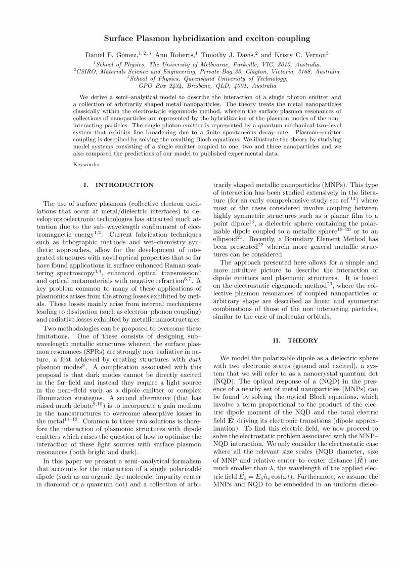
In fig. 1, we show the scattering and absorptioncross-sections calculated for systems of coupled NQD–metal nanorod. The nanorod was assumed to be ahemispherically–capped Ag cylinder of diameter 15 nmand length 80 nm, with a dielectric data for Ag that wasadapted from Johnson and Christy35. Only the longi-tudinal (dipolar) LSPR was considered, for which γmp =1.105 equivalent to a wavelength of ∼ 944 nm (1.314 eV).The dielectric spheres were assumed to have a diameterof 10 nm and a polarizabilty described by Eqn. (10) witha resonance frequency that matched that of the LSPR ofthe nanorod and a width of 5 meV [that is ω∗o = (1.314+ i0.01)eV]. The separation between the sphere and rodwas 5 nm and the polarization of the incident (uniform)electric field was assumed to be parallel to the long axisof the nanorod.

The scattering spectra shown in fig. 1 consists of a dou-blet with a “dip” located at the position of the maximumscattering intensity for the isolated nanorod. The inter-action with the NQD is said to have induced a “trans-parency” in the scattering spectrum of the nanorod.When the single rod interacts with two NQDs positionedat both ends of its tips, the induced transparency isstronger as evidenced by an increased depth in the spec-trum at the position of the LSPR of the non–interactingrod, a phenomenon that is consistent with our previousdiscussion leading to Eqn. (18).

2. “Quantum” mechanical description

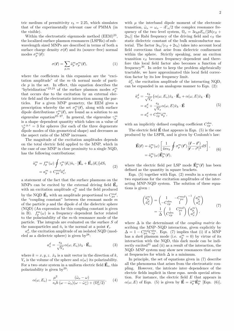
In fig. 2, we show the spectra of ~Gmp and ~Fmp calculated

(using the EEM) for a point located 20 nm away from aAg nanorod. For this nanorod, the spectrum of the z–

component of ~Gmp is composed of two resonance features

(at 943 and 477 nm), both corresponding to modes thatcan be excited by an incident uniform electric field. On

the other hand, the spectrum of the z–component of ~Fmpshows one additional resonance at 581 nm that corre-sponds to the first quadrupole–like mode of the nanorod.This mode is characterized by having ~pmp = 0 and there-

fore does not contribute to ~Gmp (see Eqn. (28)).

6

FIG. 1: (Top) Spectra of the normalised scattering (Cs) andabsorption (Ca) cross sections for a coupled systems consist-ing of a single NQD with a single nanorod as indicated in theinset. (Bottom) Spectra of the normalised scattering (Cs)cross-section for a system comprised of two non–interactingNQDs with a single nanorod (shaded plot) arranged as shownin the inset. Also shown for comparison, is the spectrum ofthe case of a single NQD–nanorod case (line)

400 500 600 700 800 900 1000 1100 1200

−20

−10

0

10

Gz

400 500 600 700 800 900 1000 1100 1200

−0.1

−0.05

0

0.05

µ2Fzn(m

eV)

Wavelength (nm)

ReIm

FIG. 2: Plots of z components of (Top) ~G and (Bottom) ~F(assumed µ = 1 e nm) calculated for a point located 20 nmaway on the z plane from the tip of a 80 nm long, 15 nm indiameter Ag nanorod with εb = 2.25 (The z axis coincideswith long axis of the nanorod). The dielectric data of ref.35

for Ag was used, and the first three LSP modes of the nanorodwere taken into account [γm1

NR = 1.105 (477 nm), γm2NR = 1.358

(582 nm), γm3NR = 1.713 (943 nm)]. Also shown in the bottom

are the surface charge distributions σmNR of each of the modes

considered. The arrows on the top panel indicate the positionof the scattering spectrum calculated with COMSOL (485 nm,595 nm and 995 nm).

These results have also been compared to finite elementfull–field simulations implemented in COMSOL Multi-physics and the spectral position of the maximma in thetotal radiated power. However, the position of the max-imum in the spectrum (longitudinal dipole mode) is lo-cated at 995 nm (shown with an arrow in 2) as opposedto the 943 nm predicted by the EEM. This discrepancyarises from the inclusion of retardation effects in the finiteelement calculations.

In fig. 3, we show the calculated excited state popula-tion of a fictitious NQD positioned 20 nm away from oneof the end tips of a Ag nanorod (same dimensions andorientation as in fig. 2). For this calculation we have as-sumed the NQD’s exciton transition to be resonant withthe longitudinal dipole–like mode of the nanorod and fur-thermore, we have also assumed the NQDs excited statedipole to be parallel to the long axis of the nanorod. Un-der these conditions and according to fig. 2 and Eqn.(31) the main effect of the surface plasmon modes of thenanorod on the NQD is to enhance the excitation rate

via an enhancement of the local electric field ~E [Eqn.

(27)] accounted for by the magnitude of ~Gmp . As shown

in this figure, the interaction leads to an enhancement ofthe excited state population.

7

800 850 900 950 1000 1050 1100

1

2

3

4

5

6

7

8

9

x 10−3

Wavelength (nm)

ρ22

iso

int

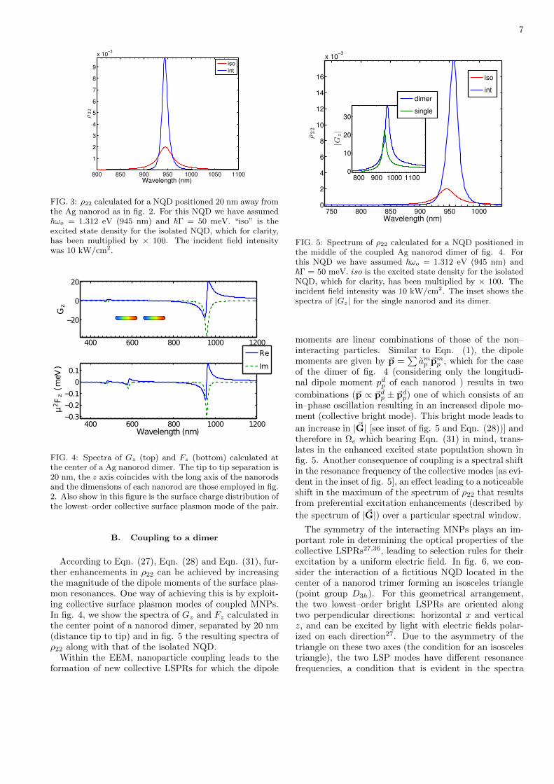
FIG. 3: ρ22 calculated for a NQD positioned 20 nm away fromthe Ag nanorod as in fig. 2. For this NQD we have assumed~ωo = 1.312 eV (945 nm) and ~Γ = 50 meV. “iso” is theexcited state density for the isolated NQD, which for clarity,has been multiplied by × 100. The incident field intensitywas 10 kW/cm2.

400 600 800 1000 1200

−20

0

20

Gz

400 600 800 1000 1200−0.3

−0.2

−0.1

0

0.1

µ2Fz(m

eV)

Wavelength (nm)

Re

Im

FIG. 4: Spectra of Gz (top) and Fz (bottom) calculated atthe center of a Ag nanorod dimer. The tip to tip separation is20 nm, the z axis coincides with the long axis of the nanorodsand the dimensions of each nanorod are those employed in fig.2. Also show in this figure is the surface charge distribution ofthe lowest–order collective surface plasmon mode of the pair.

B. Coupling to a dimer

According to Eqn. (27), Eqn. (28) and Eqn. (31), fur-ther enhancements in ρ22 can be achieved by increasingthe magnitude of the dipole moments of the surface plas-mon resonances. One way of achieving this is by exploit-ing collective surface plasmon modes of coupled MNPs.In fig. 4, we show the spectra of Gz and Fz calculated inthe center point of a nanorod dimer, separated by 20 nm(distance tip to tip) and in fig. 5 the resulting spectra ofρ22 along with that of the isolated NQD.

Within the EEM, nanoparticle coupling leads to theformation of new collective LSPRs for which the dipole

750 800 850 900 950 10000

2

4

6

8

10

12

14

16

x 10−3

Wavelength (nm)

ρ22

iso

int

800 900 1000 11000

10

20

30

|Gz|

dimer

single

FIG. 5: Spectrum of ρ22 calculated for a NQD positioned inthe middle of the coupled Ag nanorod dimer of fig. 4. Forthis NQD we have assumed ~ωo = 1.312 eV (945 nm) and~Γ = 50 meV. iso is the excited state density for the isolatedNQD, which for clarity, has been multiplied by × 100. Theincident field intensity was 10 kW/cm2. The inset shows thespectra of |Gz| for the single nanorod and its dimer.

moments are linear combinations of those of the non–interacting particles. Similar to Eqn. (1), the dipolemoments are given by ~p =

∑amp ~p

mp , which for the case

of the dimer of fig. 4 (considering only the longitudi-nal dipole moment pdp of each nanorod ) results in two

combinations (~p ∝ ~pdp ± ~pdp) one of which consists of anin–phase oscillation resulting in an increased dipole mo-ment (collective bright mode). This bright mode leads to

an increase in |~G| [see inset of fig. 5 and Eqn. (28))] andtherefore in Ωe which bearing Eqn. (31) in mind, trans-lates in the enhanced excited state population shown infig. 5. Another consequence of coupling is a spectral shiftin the resonance frequency of the collective modes [as evi-dent in the inset of fig. 5], an effect leading to a noticeableshift in the maximum of the spectrum of ρ22 that resultsfrom preferential excitation enhancements (described by

the spectrum of |~G|) over a particular spectral window.

The symmetry of the interacting MNPs plays an im-portant role in determining the optical properties of thecollective LSPRs27,36, leading to selection rules for theirexcitation by a uniform electric field. In fig. 6, we con-sider the interaction of a fictitious NQD located in thecenter of a nanorod trimer forming an isosceles triangle(point group D3h). For this geometrical arrangement,the two lowest–order bright LSPRs are oriented alongtwo perpendicular directions: horizontal x and verticalz, and can be excited by light with electric fields polar-ized on each direction27. Due to the asymmetry of thetriangle on these two axes (the condition for an isoscelestriangle), the two LSP modes have different resonancefrequencies, a condition that is evident in the spectra

8

850 900 950 1000 1050

10

20

30

40

50

G

850 900 950 1000 1050

−0.2

0

0.2

0.4

µ2Fn(m

eV)

850 900 950 1000 10500

0.05

0.1

Wavelength (nm)

ρ22

x

z

FIG. 6: Response of a NQD [~ωo = 1.277 eV (971 nm), ~Γo

= 25 meV, µ = 1 enm] positioned in the center of a trimerof nanorods (same dimensions as in fig. 2). The nanorodsform an isosceles triangle and have two collective brigth LPSmodes shown in the top. (Top) Plot of the magnitude of ~G forillumination with x and z polarized light. (Middle) Plot of the

real and imaginary (dotted line) of µ2~Fn/~. (Bottom) Plotsof the resulting spectra of the excited state population alongwith the one for the isolated NQD (black line, multiplied by1000 for clarity)

of ~G. If the NQD’s exciton transition spectrum encom-passes these two LSP modes as is shown in fig. 6 (bot-tom), then as the incident polarization is changed from xto z polarized, the MNP–NQD interaction would lead toa ρ22 that exhibits a peak amplitude on the red and blueend of the isolated NQD spectrum. This optical effectcan be achieved with NQDs due to the isotropy of theirexcitation dipole moment37.

C. Effect of ~F

In the structures considered so far, the magnitude of

µ2~Fn/~ has been considerably smaller than the linewidthof the exciton transition, resulting in almost negligible ef-

fects from this interaction pathway. The effect of ~F onthe excited state population is non–linear and intensity

dependent. According to Eqn. (31), it modifies ρ22 intwo ways: it can lead to spectral shifts and it can mod-ify the decay rate of the NQD, both effects described by

the real and imaginary parts of µ2~Fn/~, which dependon n = 2ρ22 − 1 and therefore on the intensity of theapplied field. For a plasmonic structure supporting dark

modes, according to Eqn. (28) ~G = 1 and ~F has a spec-trum whose lineshape is given by Eqn. (12) but with amagnitude dictated by the geometry of the MNP and theMNP–NQD coupled system.

In fig. 7, we show the effect of an artificial spectrum of

µ2~F/~ that was modeled to have a Lorentzian lineshapecentered on the exciton transition energy of the NQD butwhose magnitude was varied between 2Γ and Γ/4. In thissituation, ρ22(ω = ωo) = |~Ωe|2/[(~Γc/2)2 + 2|~Ωe|2],which attains a maximum value of 1/2 when Γc = 0 orwhen the coupling of the NQD to the LSPR leads to aloss compensation (|Γ/2 + µ2Im(F )n/~|2 = 0).

850 900 950 1000 1050

0.05

0.1

0.15

0.2

0.25

Wavelength (nm)

ρ22

iso

Γ/2

Γ/4

Γ

2Γ

nxΓ/2

950 960 970

FIG. 7: Effect of the peak amplitude (indicated in the legend)

of µ2~Fn/~ on the spectrum of ρ22. “iso” refers to the isolatedNQD. For this calculation we have assumed µ = 10 e nm, I= 1 kW/cm2 and ~Γ = 5 meV, nx = 1.74

As can be seen in fig. 7, if the magnitude of µ2~Fn/~is larger than Γ, the MNP–NQD interaction leads toquenching of the excited state population. Physically,this results from an increased value of Γc which is inter-preted as an increase in energy dissipation in the NQDdue to energy transfer to surface plasmon modes in theMNP. At the other extreme, maximum enhancement is

observed at a peak amplitude of µ2~Fn/~ that is slightlylarger than Γ/2 (the line labeled nxΓ/2 on the figure).The enhancement is accompanied with a significant de-crease in the spectral linewidth but the maximum valueof ρ22 attained is still well below the 1/2 limit. This

9

effect is independent of the linewidth of the function ~Fbut depends strongly on the position of its resonance asdemonstrated by the results of fig. 8.

850 900 950 1000 1050

0.002

0.004

0.006

0.008

0.01

0.012

0.014

0.016

0.018

0.02

Wavelength (nm)

ρ22

+ Γ/2

− Γ/2

res

940 950 960 970

FIG. 8: Effect of the resonance wavelength of the function ~Fon the spectra of ρ22. Three cases are plotted and they consistof (i) a blue–shift of Γ/2 in ~F, (ii) a red shift by the sameamount and (iii) the case of resonance considered already infig. 7. All the numerical parameters remained unchangedfrom those employed previously

D. Comparison with experimental results

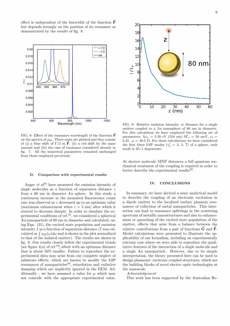
Anger et al34 have measured the emission intensity ofsingle molecules as a function of separation distance zfrom a 80 nm in diameter Au sphere. In this study acontinuous increase in the measured fluorescence countrate was observed as z decreased up to an optimum value(maximum enhancement when z = 5 nm) after which itstarted to decrease sharply. In order to simulate the ex-perimental conditions of ref.34, we considered a sphericalAu nanoparticle of 80 nm in diameter and calculated, us-ing Eqn. (31), the excited state population and emissionintensity I as a function of separation distance (I was cal-culated as

∫ρ22(ω)dω and is shown in the plot normalized

to that of the isolated emitter). The results are shown infig. 9. Our results closely follow the experimental trends[see figure 4(a) of ref.34] albeit with an optimum distancethat is about 50% smaller. Failure to reproduce the ex-perimental data may arise from our complete neglect ofsubstrate effects, which are known to modify the LSPresonances of nanoparticles38, retardation and radiativedamping which are implicitly ignored in the EEM. Ad-ditionally , we have assumed a value for µ which maynot coincide with the appropriate experimental value.

FIG. 9: Relative emission intensity vs distance for a singleemitter coupled to a Au nanosphere of 80 nm in diameter.For this calculation we have employed the following set ofparameters: ~ωo = 2.39 eV (518 nm) ~Γo = 50 meV, εb =2.25. µ = 48.5 D. For these calculations we have consideredthe first three LSP modes (γl

p = 3, 5, 7) of a sphere, eachmode is 2l+1 degenerate.

At shorter molecule–MNP distances a full quantum me-chanical treatment of the coupling is required in order tobetter describe the experimental results39.

IV. CONCLUSIONS

In summary, we have derived a semi–analytical modelto describe the coupling of an electronic excitation ina dipole emitter to the localized surface plasmon reso-nances of collection of metal nanoparticles. This inter-action can lead to resonance splittings in the scatteringspectrum of metallic nanostructures and also to enhance-ment or quenching of the excited state population of theemitter, effects that arise from a balance between the

relative contributions from a pair of functions ~G and ~F.Model calculations were presented to illustrate the ap-plicability of our formalism, including an experimentallyrelevant case where we were able to reproduce the quali-tative features of the interaction of a single molecule anda single Au nanoparticle. However, due to its simpleinterpretation, the theory presented here can be used todesign plasmonic–excitonic coupled structures, which arethe building blocks of novel electro–optic technologies atthe nanoscale.AcknowledgementThis work has been supported by the Australian Re-

10

search Council under DP110101767, DP110101454 andDP110100221. D. E. G. would also like to acknowledge

the Melbourne Materials Institute.

∗ Electronic address: [email protected] S. Maier. Plasmonics: fundamentals and applications

(Springer, New York, 2007).2 W. L. Barnes, A. Dereux and T. W. Ebbesen. Nature 424, 824

(2003).3 M. Moskovits et al. Topics in Applied Physics 82, 215 (2002).4 A. M. Michaels, Jiang and L. Brus. The Journal of Physical

Chemistry B 104, 11965 (2000).5 T. W. Ebbesen et al. Nature 391, 667 (1998).6 V. Shalaev et al. Optics Letters 30, 3356 (2005).7 V. Shalaev. Nature Photonics 1, 41 (2007).8 N. Liu et al. Nat Mater 8, 758 (2009).9 J. B. Pendry and S. A. Maier. Phys. Rev. Lett. 107, 259703

(2011).10 S. Wuestner et al. Phys. Rev. Lett. 107, 259701 (2011).11 S. Wuestner et al. Phys. Rev. Lett. 105, 127401 (2010).12 I. De Leon and P. Berini. Nat Photon 4, 382 (2010).13 M. I. Stockman. Physical Review Letters 106 (2011).14 R. R. Chance, A. Prock and R. Silbey. In “Advances in Chemical

Physics,” , edited by S. A. R. I. Prigogine, volume 37, 1–65(Wiley InterScience, 1978).

15 W. Zhang, A. O. Govorov and G. W. Bryant. Physical ReviewLetters 97, 146804 (2006).

16 A. Govorov et al. Nano Letters 6, 984 (2006).17 A. O. Govorov, J. Lee and N. A. Kotov. Physical Review B 76,

125308 (2007).18 J.-Y. Yan et al. Physical Review B 77, 165301 (2008).19 R. D. Artuso and G. W. Bryant. Nano Letters (2008).20 S. M. Sadeghi. Phys. Rev. B 79, 233309 (2009).21 T. Ambjornsson et al. Physical Review B 73, 085412 (2006).22 R. D. Artuso et al. Phys. Rev. B 83, 235406 (2011).23 T. J. Davis, D. E. Gomez and K. C. Vernon. Nano Letters 10,

2618 (2010).24 E. Prodan et al. Science 302, 419 (2003).25 I. D. Mayergoyz, D. R. Fredkin and Z. Zhang. Phys. Rev. B 72,

155412 (2005).26 T. J. Davis, K. C. Vernon and D. E. Gomez. Phys. Rev. B 79,

155423 (2009). [also in: Vir. J. Nan. Sci. & Tech. Vol. 19 (17)(2009)].

27 D. E. Gomez, K. C. Vernon and T. J. Davis. Phys. Rev. B 81,075414 (2010).

28 T. J. Davis, D. E. Gomez and K. C. Vernon. Phys. Rev. B81, 045432 (2010). Also in: Vir. J. Nan. Sci. & Tech. Vol.21(7)2010.

29 C. Cohen-Tannoudji, J. Dupont-Roc and G. Grynberg. Atom-photon interactions (John Wiley & Sons, 1998).

30 D. Ricard, M. Ghanassi and M. Schanne-Klein. Optics Com-munications 108, 311 (1994).

31 M. Liu et al. Physical Review Letters 102, 107401 (2009).32 C. M. Bowden and J. P. Dowling. Phys. Rev. A 47, 1247 (1993).33 M. E. Crenshaw and C. M. Bowden. Phys. Rev. A 53, 1139

(1996).34 P. Anger, P. Bharadwaj and L. Novotny. Physical Review Let-

ters 96, 113002 (2006).35 P. B. Johnson and R. W. Christy. Phys. Rev. B 6, 4370 (1972).36 D. W. Brandl, N. A. Mirin and P. Nordlander. The Journal of

Physical Chemistry B 110, 12302 (2006).37 A. I. Chizhik et al. Nano Letters 11, 1131 (2011).38 K. C. Vernon et al. Nano Letters 10, 2080 (2010).39 A. Manjavacas, F. J. G. d. Abajo and P. Nordlander. Nano

Letters 11, 2318 (2011).

Appendix A: The EEM

The surface plasmon eigenmodes of the MNPs werecalculated by numerically solving the eigenproblem:

σmp (~r) =γmp2π

∮σmp (~rq)

(~r−~rq)|r − rq|3

· n dSq, (A1)

where γmp are the eigenvalues that are related to the res-onance wavelength of the surface plasmon modes by:

εM (λmp ) = εb1 + γmp1− γmp

, (A2)

with λmp given by the real part of this Eqn. Here, λmp isthe wavelength of the surface plasmon resonance, εM (λ)is the (wavelength dependent) permittivity of the metaland εb that of the (uniform) background medium. Fora single spherical nanoparticle γm=1

p = 3 (dipolar mode,

triply degenerate. γm=2p = 5 corresponds to a qudrupolar

mode with 5–fold degeneracy) and this equation reducesto the familiar resonance condition εM (λ) = −2εb (TheFrolich mode). A similar eigenvalue Eqn. also exists forthe surface dipole distributions τmp (~r)23,26.

Once the set of σmp (~r) and τmp (~r) are known, the excita-tion amplitudes amp are calculated for a given polarization

of the applied electric field ~Eo.

Appendix B: Electric field radiated by the NQD andthe excitation of LSPRs

In the near–field approximation (i.e. when the wave-length of the driving field is larger than any other relevantsize scale) the electric field radiated by the NQD’s dipolemoment ~px is given by:

~Edx(~r) =

3(~px · n)n− ~px4πεb |~R−~r|3

, (B1)

with n a normal vector pointing on the direction of the

separation distance between the location of the NQD (~R)and the point of observation (~r). This expression can beinserted into Eqn. (2) resulting in:

fmp (ω)

∮τmp (~ri)[

3(~px · n)ni · n− ni · ~px4πεb |~R−~r|3

]dS = Cmdpx adx

(B2)where we have written ~px = asx~p

dx in accordance with

section II A 2.From this last result, one can infer by inspection that

the coupling coefficient can be factored out as a product

11

of a frequency–dependent component and a geometricalcomponent:

Cmdpx =fmp (ω)

4πεbGmdpx

=fmp (ω)

4πεb

∮τmp (~ri)[

3(~pdx · n)ni · n− ni · ~pdx|~R−~r|3

]dS

(B3)