Surface Integrity on Grinding of Gamma Titanium Aluminide Intermetallic Compounds A Thesis Presented to The Academic Faculty by Gregorio Roberto Murtagian In Partial Fulfillment of the Requirements for the Degree Doctor of Philosophy G.W.Woodruff School of Mechanical Engineering Georgia Institute of Technology August 2004

Welcome message from author
This document is posted to help you gain knowledge. Please leave a comment to let me know what you think about it! Share it to your friends and learn new things together.
Transcript
Surface Integrity on Grinding of Gamma Titanium Aluminide
Intermetallic Compounds
A ThesisPresented to
The Academic Faculty
by
Gregorio Roberto Murtagian
In Partial Fulfillmentof the Requirements for the Degree
Doctor of Philosophy
G.W.Woodruff School of Mechanical EngineeringGeorgia Institute of Technology
August 2004
Surface Integrity on Grinding of Gamma Titanium Aluminide
Intermetallic Compounds
Approved by:
Professor Steven Danyluk, Committee Chair
Professor David McDowell(ME-MSE)
Dr. Hugo Ernst(CINI-TENARIS)
Professor Ashok Saxena(UARK-ME)
Professor Carlos Santamarina(CE)
Professor Thomas Kurfess(ME)
Date Approved: 3 August 2004

. . . to my parents Sergio and Vera, who taught me the value of hard work and the meaning
of unconditional love
. . . to my beloved cheerleaders Veronica and Camila who fill my life with enjoyment
iii
ACKNOWLEDGEMENTS
This thesis would have not been possible without the support and confidence of my advisor. My
special thanks to Dr. S. Danyluk for accepting me as his student and giving me his confidence. I
enjoyed a truly doctoral scholar experience under his guidance and support. I would like to thank
the rest of the committee members, Dr. H. Ernst, Dr. D. McDowell, Dr. A. Saxena, Dr. C. Santa-
marina, and Dr. T. Kurfess for their time, and valuable comments to improve the quality of this
work.
I would like to thank Dr. A. Sarce, Dr. A. Pignotti, and Dr. J. Garcia Velasco for their confidence
and support to pursue this path. I also appreciate the financial support given by CINI-TENARIS.
I would like to thank Dr. P. McQuay and Dr. D. Lee from Howmet Castings for providing the
TiAl slabs used for this work. Also, to Dr. B. Varghese from GE Superabrasives for providing the
diamond abrasives, and to Dr. M. Dvoretsky from Noritake Abrasives for the manufacturing the
wheels.
I appreciate the help provided by the ORNL HTML personnel, in particular Dr. T. Watkins,
B. Kevin, Dr. E. Lara-Curzio, Dr. L. Riester, Dr. M. Ferber, and Dr. P. Blau.
I would like to thank D. Rogers, G. Payne, N. Moody, L. Teasley, S. Sheffield, V. Bortkevich,
J. Witzel, S. Schulte, J. Donnell, and D. Osorno for their kindness and willingness to help.
I have enjoyed very interesting discussions with Dr. R. Hecker, Dr. P. Jones, M. Shenoy,
J. Mayeur, Dr. R. McGinty, A. Caccialupi, B. Hagege, and many others that were very helpful
for a better understanding of grinding and modeling.
I would like to thank all my office mates, in particular Inho Yoon, for his unconditional friendship
and collaboration, and with whom I enjoyed fantastic jam sessions of chamber music. Finally, I
appreciate the fun and entertainment I had playing soccer with the “burros”.
iv
TABLE OF CONTENTS
DEDICATION . . . . . . . . . . . . . . . . . . . . . . . . . . . . . . . . . . . . . . . . . . . iii
ACKNOWLEDGEMENTS . . . . . . . . . . . . . . . . . . . . . . . . . . . . . . . . . . . iv
LIST OF TABLES . . . . . . . . . . . . . . . . . . . . . . . . . . . . . . . . . . . . . . . . ix
LIST OF FIGURES . . . . . . . . . . . . . . . . . . . . . . . . . . . . . . . . . . . . . . . xi
LIST OF SYMBOLS AND ABBREVIATIONS . . . . . . . . . . . . . . . . . . . . .xvii
SUMMARY . . . . . . . . . . . . . . . . . . . . . . . . . . . . . . . . . . . . . . . . . . . . .xxv
I INTRODUCTION . . . . . . . . . . . . . . . . . . . . . . . . . . . . . . . . . . . . . . 1
1.1 Historical Perspective . . . . . . . . . . . . . . . . . . . . . . . . . . . . . . . . . . . 1
1.2 Gamma-TiAl . . . . . . . . . . . . . . . . . . . . . . . . . . . . . . . . . . . . . . . 2
1.2.1 Phase Diagram and Microstructure . . . . . . . . . . . . . . . . . . . . . . . 2
1.2.2 Thermal Treatment and Alloys . . . . . . . . . . . . . . . . . . . . . . . . . 4
1.2.3 Deformation Mechanisms . . . . . . . . . . . . . . . . . . . . . . . . . . . . . 6
1.3 Grinding . . . . . . . . . . . . . . . . . . . . . . . . . . . . . . . . . . . . . . . . . . 8
1.4 Effects of Machining on Gamma-TiAl . . . . . . . . . . . . . . . . . . . . . . . . . . 11
1.5 Surface Integrity Evaluation . . . . . . . . . . . . . . . . . . . . . . . . . . . . . . . 12
1.5.1 Plastic Deformation Depth Measurement . . . . . . . . . . . . . . . . . . . . 13
II PRESENT WORK . . . . . . . . . . . . . . . . . . . . . . . . . . . . . . . . . . . . . 15
2.1 Motivation . . . . . . . . . . . . . . . . . . . . . . . . . . . . . . . . . . . . . . . . . 15
2.2 Objective . . . . . . . . . . . . . . . . . . . . . . . . . . . . . . . . . . . . . . . . . . 17
2.3 Methodology and Outline . . . . . . . . . . . . . . . . . . . . . . . . . . . . . . . . . 17
III MATERIAL CHARACTERIZATION . . . . . . . . . . . . . . . . . . . . . . . . . 19
3.1 Chemical Composition and Metallography . . . . . . . . . . . . . . . . . . . . . . . 19
3.2 Elastic Constants . . . . . . . . . . . . . . . . . . . . . . . . . . . . . . . . . . . . . 21
3.3 Quasi-static and Dynamic Compression Tests . . . . . . . . . . . . . . . . . . . . . 25
3.4 Indentation Tests . . . . . . . . . . . . . . . . . . . . . . . . . . . . . . . . . . . . . 28
IV PLASTIC DEFORMATION DEPTH MEASUREMENT METHOD . . . . . . 30
4.1 Introduction . . . . . . . . . . . . . . . . . . . . . . . . . . . . . . . . . . . . . . . . 30
v
4.2 Background of Method . . . . . . . . . . . . . . . . . . . . . . . . . . . . . . . . . . 31
4.3 Proposed Method . . . . . . . . . . . . . . . . . . . . . . . . . . . . . . . . . . . . . 32
4.3.1 Consistency of Results . . . . . . . . . . . . . . . . . . . . . . . . . . . . . . 32
4.4 Data Analysis . . . . . . . . . . . . . . . . . . . . . . . . . . . . . . . . . . . . . . . 34
4.5 Capabilities and Limitations of the Method . . . . . . . . . . . . . . . . . . . . . . 35
4.6 Conclusions . . . . . . . . . . . . . . . . . . . . . . . . . . . . . . . . . . . . . . . . 36
V GRINDING EXPERIMENTS . . . . . . . . . . . . . . . . . . . . . . . . . . . . . . 40
5.1 Introduction . . . . . . . . . . . . . . . . . . . . . . . . . . . . . . . . . . . . . . . . 40
5.2 Design of Experiments . . . . . . . . . . . . . . . . . . . . . . . . . . . . . . . . . . 40
5.3 Wheel Characteristics . . . . . . . . . . . . . . . . . . . . . . . . . . . . . . . . . . . 41
5.4 Consistency of Results . . . . . . . . . . . . . . . . . . . . . . . . . . . . . . . . . . 41
5.4.1 Wheel Wear . . . . . . . . . . . . . . . . . . . . . . . . . . . . . . . . . . . . 43
5.4.2 Dressing Conditions . . . . . . . . . . . . . . . . . . . . . . . . . . . . . . . . 44
5.4.3 Coolant . . . . . . . . . . . . . . . . . . . . . . . . . . . . . . . . . . . . . . 44
5.4.4 Hydrodynamic Effects . . . . . . . . . . . . . . . . . . . . . . . . . . . . . . 46
5.5 Wheel Conditioning . . . . . . . . . . . . . . . . . . . . . . . . . . . . . . . . . . . . 47
5.6 Grinder and Data Acquisition . . . . . . . . . . . . . . . . . . . . . . . . . . . . . . 47
5.7 Results . . . . . . . . . . . . . . . . . . . . . . . . . . . . . . . . . . . . . . . . . . . 50
5.7.1 Dressed Wheels . . . . . . . . . . . . . . . . . . . . . . . . . . . . . . . . . . 50
5.7.2 Worn Wheels . . . . . . . . . . . . . . . . . . . . . . . . . . . . . . . . . . . 54
5.7.3 All Wheels . . . . . . . . . . . . . . . . . . . . . . . . . . . . . . . . . . . . . 67
5.8 Conclusions . . . . . . . . . . . . . . . . . . . . . . . . . . . . . . . . . . . . . . . . 74
5.8.1 PDD . . . . . . . . . . . . . . . . . . . . . . . . . . . . . . . . . . . . . . . . 77
5.8.2 Grinding Friction Coefficient . . . . . . . . . . . . . . . . . . . . . . . . . . . 78
5.8.3 Specific Normal Force . . . . . . . . . . . . . . . . . . . . . . . . . . . . . . . 78
5.8.4 Surface Parameters . . . . . . . . . . . . . . . . . . . . . . . . . . . . . . . . 78
5.8.5 Cracking . . . . . . . . . . . . . . . . . . . . . . . . . . . . . . . . . . . . . . 79
VI RESIDUAL STRESS MEASUREMENTS . . . . . . . . . . . . . . . . . . . . . . . 80
6.1 Introduction . . . . . . . . . . . . . . . . . . . . . . . . . . . . . . . . . . . . . . . . 80
6.2 Design of Experiments . . . . . . . . . . . . . . . . . . . . . . . . . . . . . . . . . . 81
vi
6.3 Experimental Technique . . . . . . . . . . . . . . . . . . . . . . . . . . . . . . . . . 81
6.4 Data Analysis . . . . . . . . . . . . . . . . . . . . . . . . . . . . . . . . . . . . . . . 88
6.5 Results . . . . . . . . . . . . . . . . . . . . . . . . . . . . . . . . . . . . . . . . . . . 94
6.6 Conclusions . . . . . . . . . . . . . . . . . . . . . . . . . . . . . . . . . . . . . . . . 95
VII ANALYTICAL MODELING . . . . . . . . . . . . . . . . . . . . . . . . . . . . . . . 101
7.1 Indentation Model . . . . . . . . . . . . . . . . . . . . . . . . . . . . . . . . . . . . . 101
7.2 Force per Abrasive Model . . . . . . . . . . . . . . . . . . . . . . . . . . . . . . . . 102
7.3 Implementation . . . . . . . . . . . . . . . . . . . . . . . . . . . . . . . . . . . . . . 106
7.4 Results . . . . . . . . . . . . . . . . . . . . . . . . . . . . . . . . . . . . . . . . . . . 108
7.4.1 Dressed Wheel Tests . . . . . . . . . . . . . . . . . . . . . . . . . . . . . . . 108
7.4.2 Worn Wheel Tests . . . . . . . . . . . . . . . . . . . . . . . . . . . . . . . . 109
7.5 Conclusions . . . . . . . . . . . . . . . . . . . . . . . . . . . . . . . . . . . . . . . . 114
VIIINUMERICAL MODELING . . . . . . . . . . . . . . . . . . . . . . . . . . . . . . . 121
8.1 Isotropic Elastic-plastic Model Simulations . . . . . . . . . . . . . . . . . . . . . . . 121
8.1.1 Model Validation . . . . . . . . . . . . . . . . . . . . . . . . . . . . . . . . . 121
8.1.2 3D Scratching . . . . . . . . . . . . . . . . . . . . . . . . . . . . . . . . . . . 122
8.1.3 Plane Strain vs. Plane Stress Comparison . . . . . . . . . . . . . . . . . . . 124
8.2 Hyperelastic Model . . . . . . . . . . . . . . . . . . . . . . . . . . . . . . . . . . . . 129
8.3 Material Properties . . . . . . . . . . . . . . . . . . . . . . . . . . . . . . . . . . . . 133
8.3.1 Elastic Constants . . . . . . . . . . . . . . . . . . . . . . . . . . . . . . . . . 133
8.3.2 Planar Triple Slip . . . . . . . . . . . . . . . . . . . . . . . . . . . . . . . . . 134
8.3.3 Visco-plastic Parameters Calibration . . . . . . . . . . . . . . . . . . . . . . 135
8.4 Implementation and Results . . . . . . . . . . . . . . . . . . . . . . . . . . . . . . . 136
8.5 Conclusions . . . . . . . . . . . . . . . . . . . . . . . . . . . . . . . . . . . . . . . . 137
IX DISCUSSION . . . . . . . . . . . . . . . . . . . . . . . . . . . . . . . . . . . . . . . . 141
9.1 Grinding . . . . . . . . . . . . . . . . . . . . . . . . . . . . . . . . . . . . . . . . . . 141
9.2 PDD Controlling Factors . . . . . . . . . . . . . . . . . . . . . . . . . . . . . . . . . 142
9.3 Force per Grit Analytical Model . . . . . . . . . . . . . . . . . . . . . . . . . . . . . 142
9.4 Significance of PDD Measurement Technique . . . . . . . . . . . . . . . . . . . . . . 145
9.4.1 Significance as PDD Evaluation Method . . . . . . . . . . . . . . . . . . . . 145
vii
9.4.2 Significance in Terms of Mechanical Performance . . . . . . . . . . . . . . . 145
9.4.3 Relation with PDD at Bulk . . . . . . . . . . . . . . . . . . . . . . . . . . . 146
9.4.4 PDD, Microstructure, and Cracking . . . . . . . . . . . . . . . . . . . . . . . 146
9.4.5 Scratching Model and Indentation Model . . . . . . . . . . . . . . . . . . . . 147
9.5 Residual Stress . . . . . . . . . . . . . . . . . . . . . . . . . . . . . . . . . . . . . . 148
X CONCLUSIONS AND RECOMMENDATIONS . . . . . . . . . . . . . . . . . . . 149
10.1 Conclusions . . . . . . . . . . . . . . . . . . . . . . . . . . . . . . . . . . . . . . . . 149
10.1.1 PDD Evaluation Technique . . . . . . . . . . . . . . . . . . . . . . . . . . . 149
10.1.2 Grinding . . . . . . . . . . . . . . . . . . . . . . . . . . . . . . . . . . . . . . 149
10.1.3 Residual Stresses . . . . . . . . . . . . . . . . . . . . . . . . . . . . . . . . . 152
10.1.4 Analytical Modeling . . . . . . . . . . . . . . . . . . . . . . . . . . . . . . . 152
10.1.5 Numerical Modeling . . . . . . . . . . . . . . . . . . . . . . . . . . . . . . . 153
10.2 Recommendations . . . . . . . . . . . . . . . . . . . . . . . . . . . . . . . . . . . . . 153
APPENDIX A — GRINDING EXPERIMENTAL RESULTS . . . . . . . . . . . 156
APPENDIX B — RESIDUAL STRESS MEASUREMENT RESULTS . . . . . 183
REFERENCES . . . . . . . . . . . . . . . . . . . . . . . . . . . . . . . . . . . . . . . . . . 227
VITA . . . . . . . . . . . . . . . . . . . . . . . . . . . . . . . . . . . . . . . . . . . . . . . . . 236
viii

LIST OF TABLES
Table 3.1 Elastic constants. . . . . . . . . . . . . . . . . . . . . . . . . . . . . . . . . . . . . 22
Table 5.1 DOE for grinding tests. . . . . . . . . . . . . . . . . . . . . . . . . . . . . . . . . . 40
Table 5.2 Truing conditions . . . . . . . . . . . . . . . . . . . . . . . . . . . . . . . . . . . . 48
Table 5.3 Dressing conditions . . . . . . . . . . . . . . . . . . . . . . . . . . . . . . . . . . . 48
Table 5.4 Summary for tests using dressed wheels. . . . . . . . . . . . . . . . . . . . . . . . 51
Table 5.5 Bonferroni test for homogeneous groups for dressed conditions . . . . . . . . . . . 51
Table 5.6 ANOVA for the PDD. . . . . . . . . . . . . . . . . . . . . . . . . . . . . . . . . . 53
Table 5.7 Stepwise regression model for PDD. . . . . . . . . . . . . . . . . . . . . . . . . . . 53
Table 5.8 Best subset regression model for Cf . . . . . . . . . . . . . . . . . . . . . . . . . . 55
Table 5.9 Summary for tests using worn wheels. . . . . . . . . . . . . . . . . . . . . . . . . 59
Table 5.10 Bonferroni test for homogeneous groups for worn conditions . . . . . . . . . . . . 60
Table 5.11 ANOVA for the PDD. . . . . . . . . . . . . . . . . . . . . . . . . . . . . . . . . . 61
Table 5.12 Stepwise regression model for PDD. . . . . . . . . . . . . . . . . . . . . . . . . . . 62
Table 5.13 Best subset regression model for Cf . . . . . . . . . . . . . . . . . . . . . . . . . . 63
Table 5.14 Best subset regression model for PDD. . . . . . . . . . . . . . . . . . . . . . . . . 69
Table 5.15 ANOVA for the PDD regression model. . . . . . . . . . . . . . . . . . . . . . . . . 70
Table 6.1 DOE for residual stress measurements. . . . . . . . . . . . . . . . . . . . . . . . . 81
Table 6.2 Residual stress summary of results . . . . . . . . . . . . . . . . . . . . . . . . . . 97
Table 7.1 Fitted parameters . . . . . . . . . . . . . . . . . . . . . . . . . . . . . . . . . . . . 108
Table 8.1 Slip systems contants. . . . . . . . . . . . . . . . . . . . . . . . . . . . . . . . . . 135
Table A.1 Complete set of tests for dressed conditions . . . . . . . . . . . . . . . . . . . . . 157
Table A.2 Complete set of tests for worn conditions . . . . . . . . . . . . . . . . . . . . . . . 170
Table B.1 Tests for determination of the mean value of d224 and its deviation. . . . . . . . 184
Table B.2 Tests for determination of the mean value of d422 and its deviation. . . . . . . . 184
Table B.3 Extended summary of residual stress measurement results . . . . . . . . . . . . . 185
Table B.4 Sample X1G06 test 13733 plane 224. Surface . . . . . . . . . . . . . . . . . . . 186
Table B.5 Sample X1G06 test 13733 plane 422. Surface . . . . . . . . . . . . . . . . . . . 187
Table B.6 Sample X1G06 test 13802 plane 224. 76µm subsurface . . . . . . . . . . . . . . 189
Table B.7 Sample X1G06 test 13802 plane 422. 76µm subsurface . . . . . . . . . . . . . . 190
ix
Table B.8 Sample X1G06 test 13823 plane 422. 76µm subsurface . . . . . . . . . . . . . . 192
Table B.9 Sample X1G06 test 10273 plane 224. 254µm subsurface . . . . . . . . . . . . . 194
Table B.10 Sample X1G06 test 10273 plane 422. 254µm subsurface . . . . . . . . . . . . . 195
Table B.11 Sample X1G06 test 10318 plane 224. 318µm subsurface . . . . . . . . . . . . . 197
Table B.12 Sample X1G15 test 13836 plane 224. Surface . . . . . . . . . . . . . . . . . . . 199
Table B.13 Sample X1G15 test 13836 plane 422. Surface . . . . . . . . . . . . . . . . . . . 200
Table B.14 Sample X1G15 test 13853 plane 422. 17µm subsurface . . . . . . . . . . . . . . 202
Table B.15 Sample X1G15 test 13883 plane 224. 47µm subsurface . . . . . . . . . . . . . . 204
Table B.16 Sample X1G15 test 13883 plane 422. 47µm subsurface . . . . . . . . . . . . . . 205
Table B.17 Sample X1G15 test 13934 plane 224. 117µm subsurface . . . . . . . . . . . . . 207
Table B.18 Sample X1G10 test 13781 plane 224. 124µm subsurface . . . . . . . . . . . . . 209
Table B.19 Sample X1G10 test 13781 plane 422. 124µm subsurface . . . . . . . . . . . . . 210
Table B.20 Sample X1G10 test 13919 plane 224. 154µm subsurface . . . . . . . . . . . . . 212
Table B.21 Sample X1G10 test 13919 plane 422. 154µm subsurface . . . . . . . . . . . . . 213
Table B.22 Sample X1G10 test 13926 plane 224. 154µm subsurface . . . . . . . . . . . . . 215
Table B.23 Sample X1G10 test 13926 plane 422. 154µm subsurface . . . . . . . . . . . . . 216
Table B.24 Sample X2G08 test 13711 plane 224. Surface . . . . . . . . . . . . . . . . . . . 218
Table B.25 Sample X2G08 test 13711 plane 422. Surface . . . . . . . . . . . . . . . . . . . 219
Table B.26 Sample X2G08 test 13753 plane 224. 72µm subsurface . . . . . . . . . . . . . . 221
Table B.27 Sample X2G08 test 13753 plane 422. 72µm subsurface . . . . . . . . . . . . . . 222
Table B.28 Sample X2G08 test 10289 plane 224. 122µm subsurface . . . . . . . . . . . . . 224
Table B.29 Sample X2G08 test 10289 plane 422. 122µm subsurface . . . . . . . . . . . . . 225
x
LIST OF FIGURES
Figure 1.1 Equilibrium phase diagram of TiAl . . . . . . . . . . . . . . . . . . . . . . . . . . 3
Figure 1.2 TiAl FCT-like structure and Ti3Al HCP-like structure . . . . . . . . . . . . . . . 3
Figure 1.3 CCT curves showing the solid-solid transformation on Ti-48Al . . . . . . . . . . 6
Figure 1.4 Lamellae colony showing the α2 phase and different variants of γ phase. . . . . . 7
Figure 1.5 Potential slip and twinning systems of the L10 structure . . . . . . . . . . . . . . 7
Figure 1.6 Schematics of grinding. . . . . . . . . . . . . . . . . . . . . . . . . . . . . . . . . 8
Figure 1.7 Input/output variables in grinding . . . . . . . . . . . . . . . . . . . . . . . . . . 10
Figure 1.8 Residual stress for an AISI 4340 steel under different grinding conditions . . . . . 12
Figure 2.1 Thesis overview. . . . . . . . . . . . . . . . . . . . . . . . . . . . . . . . . . . . . 18
Figure 3.1 Equilibrium phase diagram of Ti-Al . . . . . . . . . . . . . . . . . . . . . . . . . 20
Figure 3.2 Microstructure of the utilized TiAl showing lamellae colonies . . . . . . . . . . . 20
Figure 3.3 Microstructure of the utilized TiAl showing a lamellar colony boundary. . . . . . 21
Figure 3.4 3D representation of spatial variation of elastic constants. . . . . . . . . . . . . . 24
Figure 3.5 2D representation of directional variation of elastic constants . . . . . . . . . . . 24
Figure 3.6 Split Hopkinson bar test rig. . . . . . . . . . . . . . . . . . . . . . . . . . . . . . 26
Figure 3.7 Split Hopkinson bar test rig. Close-up of sample and strain gages. . . . . . . . . 26
Figure 3.8 Strain gages signal obtained from split Hopkinson bar test. . . . . . . . . . . . . 27
Figure 3.9 True stress and strain rate vs. true strain from split Hopkinson bar test . . . . . 27
Figure 3.10 True stress vs. true strain curves . . . . . . . . . . . . . . . . . . . . . . . . . . . 28
Figure 3.11 Indentation force versus displacement load unload curves. . . . . . . . . . . . . . 29
Figure 3.12 Macrography and 3D surface profilometry of indentation edge . . . . . . . . . . . 29
Figure 4.1 Exaggerated view of burr formed at the material lateral edges . . . . . . . . . . . 31
Figure 4.2 Bonded interface technique sample schematics. . . . . . . . . . . . . . . . . . . . 32
Figure 4.3 Experimental steps to obtain the raw data to analyze PDD. . . . . . . . . . . . . 33
Figure 4.4 Lateral free surface on a sample showing different zones. . . . . . . . . . . . . . . 33
Figure 4.5 Conditioned data from 3D profilometer. . . . . . . . . . . . . . . . . . . . . . . . 35
Figure 4.6 PDD contour plot for 3, 1 and 0.25µm of threshold. . . . . . . . . . . . . . . . . 36
Figure 4.7 Plot of the mean value of the lateral material flow-datum distance. . . . . . . . . 37
Figure 4.8 Comparison of PDD for threshold values of 3µm and 1µm . . . . . . . . . . . . . 38
xi
Figure 4.9 Comparison of PDD for threshold values of 0.25µm and 1µm . . . . . . . . . . . 38
Figure 4.10 Technique limitation by data scatter . . . . . . . . . . . . . . . . . . . . . . . . . 39
Figure 4.11 Comparison of the averaging and contour plot methods . . . . . . . . . . . . . . 39
Figure 5.1 Grinding wheel diamond abrasives . . . . . . . . . . . . . . . . . . . . . . . . . . 42
Figure 5.2 Effects of abrasive wear on the normal force. . . . . . . . . . . . . . . . . . . . . 43
Figure 5.3 Normal and tangential force in a grinding cycle. . . . . . . . . . . . . . . . . . . . 44
Figure 5.4 Plot of two different tests showing the effects of dressing on the normal force. . . 45
Figure 5.5 Effect of cooling conditions on the normal force. . . . . . . . . . . . . . . . . . . 45
Figure 5.6 Nozzles modification allowing homogeneous flux on the wheel. . . . . . . . . . . . 46
Figure 5.7 Refractometer and optical scale used to measure oil concentration. . . . . . . . . 46
Figure 5.8 Effect of hydrodynamic pressure of the normal force. . . . . . . . . . . . . . . . . 46
Figure 5.9 Schematics of wheel conditioning. . . . . . . . . . . . . . . . . . . . . . . . . . . . 47
Figure 5.10 Grinding experimental setup. . . . . . . . . . . . . . . . . . . . . . . . . . . . . . 49
Figure 5.11 ANOVA plot for main effects on PDD. . . . . . . . . . . . . . . . . . . . . . . . . 52
Figure 5.12 ANOVA plot for interaction effects on PDD. . . . . . . . . . . . . . . . . . . . . 52
Figure 5.13 ANOVA plot for main effects on Cf . . . . . . . . . . . . . . . . . . . . . . . . . . 54
Figure 5.14 ANOVA plot for interaction effects on Cf . . . . . . . . . . . . . . . . . . . . . . . 55
Figure 5.15 ANOVA plot for main effects on F ′N . . . . . . . . . . . . . . . . . . . . . . . . . 56
Figure 5.16 ANOVA plot for interaction effects on F ′N . . . . . . . . . . . . . . . . . . . . . . 56
Figure 5.17 ANOVA plot for main effects on P ′w. . . . . . . . . . . . . . . . . . . . . . . . . 57
Figure 5.18 ANOVA plot for main effects on E′g. . . . . . . . . . . . . . . . . . . . . . . . . . 57
Figure 5.19 ANOVA plot for main effects on Ra. . . . . . . . . . . . . . . . . . . . . . . . . . 58
Figure 5.20 ANOVA plot for main effects on 90% BA. . . . . . . . . . . . . . . . . . . . . . . 58
Figure 5.21 ANOVA plot for main effects on PDD. . . . . . . . . . . . . . . . . . . . . . . . . 60
Figure 5.22 ANOVA plot for interaction effects on PDD. . . . . . . . . . . . . . . . . . . . . 61
Figure 5.23 ANOVA plot for main effects on Cf . . . . . . . . . . . . . . . . . . . . . . . . . . 62
Figure 5.24 ANOVA plot for interaction effects on Cf . . . . . . . . . . . . . . . . . . . . . . . 63
Figure 5.25 ANOVA plot for main effects on F ′N . . . . . . . . . . . . . . . . . . . . . . . . . 64
Figure 5.26 ANOVA plot for interaction effects on F ′N . . . . . . . . . . . . . . . . . . . . . . 65
Figure 5.27 ANOVA plot for main effects on P ′w. . . . . . . . . . . . . . . . . . . . . . . . . 65
Figure 5.28 ANOVA plot for main effects on E′g. . . . . . . . . . . . . . . . . . . . . . . . . . 66
xii
Figure 5.29 ANOVA plot for main effects on Ra. . . . . . . . . . . . . . . . . . . . . . . . . . 66
Figure 5.30 ANOVA plot for main effects on 90% BA. . . . . . . . . . . . . . . . . . . . . . . 66
Figure 5.31 Observed cracking on ground surface . . . . . . . . . . . . . . . . . . . . . . . . . 67
Figure 5.32 ANOVA plot for main effects on PDD. . . . . . . . . . . . . . . . . . . . . . . . . 68
Figure 5.33 ANOVA plot for interaction effects on PDD. . . . . . . . . . . . . . . . . . . . . 68
Figure 5.34 ANOVA plot for main effects on Cf . . . . . . . . . . . . . . . . . . . . . . . . . . 70
Figure 5.35 ANOVA plot for interaction effects on Cf . . . . . . . . . . . . . . . . . . . . . . . 71
Figure 5.36 ANOVA plot for main effects on F ′N . . . . . . . . . . . . . . . . . . . . . . . . . 71
Figure 5.37 ANOVA plot for interaction effects on F ′N . . . . . . . . . . . . . . . . . . . . . . 72
Figure 5.38 ANOVA plot for main effects on Ra. . . . . . . . . . . . . . . . . . . . . . . . . . 72
Figure 5.39 ANOVA plot for interactions on Ra. . . . . . . . . . . . . . . . . . . . . . . . . . 73
Figure 5.40 ANOVA Plot for main effects on 90% BA. . . . . . . . . . . . . . . . . . . . . . . 73
Figure 5.41 ANOVA plot for interactions on 90% BA. . . . . . . . . . . . . . . . . . . . . . . 74
Figure 5.42 Plot of mean PDD and its standard deviation vs. F ′N . . . . . . . . . . . . . . . . 75
Figure 5.43 Plot of mean PDD and its standard deviation vs. P ′w. . . . . . . . . . . . . . . . 75
Figure 5.44 Plot of mean PDD and its standard deviation vs. E′g. . . . . . . . . . . . . . . . 76
Figure 5.45 Plot of mean PDD and its standard deviation vs. Cf . . . . . . . . . . . . . . . . 76
Figure 6.1 Measurement of interplanar spacing dhkl. . . . . . . . . . . . . . . . . . . . . . 80
Figure 6.2 Angles convention. . . . . . . . . . . . . . . . . . . . . . . . . . . . . . . . . . . . 83
Figure 6.3 X-ray diffraction machine utilized for measurements. . . . . . . . . . . . . . . . . 85
Figure 6.4 X-ray diffraction machine. Close-up of mounted specimen. . . . . . . . . . . . . . 86
Figure 6.5 Calculated 2Θ vs. relative intensity. Full range . . . . . . . . . . . . . . . . . . . 87
Figure 6.6 Measured peaks in the calculated 2Θ vs. relative intensity. Range of interest. . . 88
Figure 6.7 Acquired data, partial and total fits in the 2Θ vs. relative intensity plot. . . . . . 89
Figure 6.8 Intensity absorption vs. depth. . . . . . . . . . . . . . . . . . . . . . . . . . . . . 91
Figure 6.9 Penetration depth as a function of the tilt angle . . . . . . . . . . . . . . . . . . 91
Figure 6.10 Laboratory and sample reference systems for data acquisition . . . . . . . . . . . 92
Figure 6.11 Indetermination on the orientation of the crystal normal to the diffracted plane. 94
Figure 6.12 Comparison of the theoretical strain with the measured one . . . . . . . . . . . . 96
Figure 6.13 Comparison of the theoretical strain with the measured one . . . . . . . . . . . . 96
Figure 6.14 Surface layer data where peak broadening can be observed . . . . . . . . . . . . . 97
xiii
Figure 6.15 Surface layer data. Peaks start resolving in cases of milder grinding conditions. . 97
Figure 6.16 Low intensity and resolution in 224 peak . . . . . . . . . . . . . . . . . . . . . 98
Figure 6.17 High intensity in the Kα2 secondary peaks . . . . . . . . . . . . . . . . . . . . . . 98
Figure 6.18 Contour plot of a 3D profilometry on an electro-polished specimen . . . . . . . . 98
Figure 6.19 Longitudinal residual stresses results. . . . . . . . . . . . . . . . . . . . . . . . . . 99
Figure 6.20 Residual stresses results for samples with 600µm PDD. . . . . . . . . . . . . . . . 99
Figure 6.21 Residual stresses results for samples with 200µm PDD. . . . . . . . . . . . . . . . 100
Figure 7.1 Block diagram of the grinding model . . . . . . . . . . . . . . . . . . . . . . . . . 103
Figure 7.2 Schematics of single abrasive grit material interaction. . . . . . . . . . . . . . . . 104
Figure 7.3 Schematics of the force per abrasive grit . . . . . . . . . . . . . . . . . . . . . . . 106
Figure 7.4 Exposed abrasive grits and cumulative distribution of density of cutting edges . . 107
Figure 7.5 Model dynamic and static cutting edges. Ag-dressed wheels. . . . . . . . . . . . . 109
Figure 7.6 Expected chip thickness and standard deviation. Ag-worn wheels. . . . . . . . . 110
Figure 7.7 Model and measured P ′w. Ag-dressed wheels. . . . . . . . . . . . . . . . . . . . . 110
Figure 7.8 Model and measured F ′N and F ′
T . Ag-dressed wheels. . . . . . . . . . . . . . . . . 111
Figure 7.9 Model dynamic and static cutting edges. Bk-dressed wheels. . . . . . . . . . . . . 111
Figure 7.10 Expected chip thickness and standard deviation. Bk-worn wheels. . . . . . . . . 112
Figure 7.11 Model and measured P ′w. Bk-dressed wheels. . . . . . . . . . . . . . . . . . . . . 112
Figure 7.12 Model and measured F ′N and F ′
T . Bk-dressed wheels. . . . . . . . . . . . . . . . . 113
Figure 7.13 Model average chip thickness versus mean PDD. Test with dressed wheels. . . . . 113
Figure 7.14 Model average square root of normal force per grit versus mean PDD . . . . . . 114
Figure 7.15 Model dynamic and static cutting edges. Ag-worn wheels. . . . . . . . . . . . . . 115
Figure 7.16 Expected chip thickness and standard deviation. Ag-worn wheels. . . . . . . . . 115
Figure 7.17 Model and measured P ′w. Ag-worn wheels. . . . . . . . . . . . . . . . . . . . . . . 116
Figure 7.18 Model and measured F ′N and F ′
T . Ag-worn wheels. . . . . . . . . . . . . . . . . . 116
Figure 7.19 Model dynamic and static cutting edges. Bk-worn wheels. . . . . . . . . . . . . . 117
Figure 7.20 Expected chip thickness and standard deviation. Bk-worn wheels. . . . . . . . . 117
Figure 7.21 Model and measured P ′w. Bk-worn wheels. . . . . . . . . . . . . . . . . . . . . . . 118
Figure 7.22 Model and measured F ′N and F ′
T . Bk-worn wheels. . . . . . . . . . . . . . . . . . 118
Figure 7.23 Model average chip thickness versus mean PDD. Test with worn wheels. . . . . . 119
Figure 7.24 Model average square root of normal force per grit versus mean PDD . . . . . . 119
xiv
Figure 8.1 Axisymmetric indentation model mesh and BC’c. . . . . . . . . . . . . . . . . . . 122
Figure 8.2 Axisymmetric indentation model mesh. Contact zone close-up. . . . . . . . . . . 122
Figure 8.3 PEEQ under the indenter for 500N normal load. . . . . . . . . . . . . . . . . . . 123
Figure 8.4 Experimental and numerical comparison of indentation curves . . . . . . . . . . . 123
Figure 8.5 Half of the 3D scratching model mesh. . . . . . . . . . . . . . . . . . . . . . . . . 124
Figure 8.6 Half of the 3D scratching model mesh. Close-up of sliding zone. . . . . . . . . . . 124
Figure 8.7 PEEQ under the scratching zone for 0.5µm penetration depth. . . . . . . . . . . 125
Figure 8.8 PEEQ under the scratching zone. Close-up of sliding zone . . . . . . . . . . . . . 125
Figure 8.9 PDD vs. F ′′n0.5 for different levels of PEEQ; 232µm diameter indenter. . . . . . 125
Figure 8.10 PDD vs. F ′′n0.5 for different levels of PEEQ; 54µm diameter indenter. . . . . . . 126
Figure 8.11 Two dimensional PE-PS indentation model mesh. . . . . . . . . . . . . . . . . . . 127
Figure 8.12 Two dimensional PE-PS indentation model mesh. Contact zone close-up. . . . . 127
Figure 8.13 PEEQ under the indentation zone for 1.0µm penetration depth . . . . . . . . . . 127
Figure 8.14 PEEQ under the constant indentation depth of 1.0µm . . . . . . . . . . . . . . . 128
Figure 8.15 PEEQ for 1.0µm penetration depth . . . . . . . . . . . . . . . . . . . . . . . . . 128
Figure 8.16 PEEQ under the constant indentation force of 12.4N . . . . . . . . . . . . . . . . 129
Figure 8.17 Multiplicative decomposition of the deformation gradient. . . . . . . . . . . . . . 130
Figure 8.18 Slip systems directions and slip plane normals. . . . . . . . . . . . . . . . . . . . 134
Figure 8.19 Typical representation of model used in parameters calibration . . . . . . . . . . 135
Figure 8.20 Experimental and numerical comparison of true stress vs. true strain curves. . . 136
Figure 8.21 Hexagonal lamellae colonies and mesh used for scratching tests. . . . . . . . . . . 136
Figure 8.22 Slip systems initial orientation angles. . . . . . . . . . . . . . . . . . . . . . . . . 137
Figure 8.23 Plastic deformation for small indenter . . . . . . . . . . . . . . . . . . . . . . . . 138
Figure 8.24 Plastic deformation for large indenter . . . . . . . . . . . . . . . . . . . . . . . . 139
Figure 8.25 Grain boundary and orientation effect on plastic deformation. . . . . . . . . . . . 140
Figure 9.1 Dressed and worn abrasive grit . . . . . . . . . . . . . . . . . . . . . . . . . . . . 144
Figure 9.2 Qualitative variation of Cf with Wr. . . . . . . . . . . . . . . . . . . . . . . . . . 144
Figure 9.3 Qualitative variation of P ′w with Wr. . . . . . . . . . . . . . . . . . . . . . . . . . 145
Figure 9.4 Recrystallized zone at the machined subsurface . . . . . . . . . . . . . . . . . . . 146
Figure 9.5 Plastic deformation observed on the surface grains . . . . . . . . . . . . . . . . . 147
xv
Figure B.1 Comparison of the theoretical/measured strain component for sample X1G06test 13733. Surface . . . . . . . . . . . . . . . . . . . . . . . . . . . . . . . . . . . 188
Figure B.2 Comparison of the theoretical/measured strain component for sample X1G06test 13802. 76µm subsurface . . . . . . . . . . . . . . . . . . . . . . . . . . . . . . 191
Figure B.3 Comparison of the theoretical/measured strain component for sample X1G06test 13823 plane 422. 76µm subsurface . . . . . . . . . . . . . . . . . . . . . . 193
Figure B.4 Comparison of the theoretical/measured strain component for sample X1G06test 10273. 254µm subsurface . . . . . . . . . . . . . . . . . . . . . . . . . . . . . 196
Figure B.5 Comparison of the theoretical/measured strain component for sample X1G06test 10318 plane 224. 318µm subsurface . . . . . . . . . . . . . . . . . . . . . . 198
Figure B.6 Comparison of the theoretical/measured strain component for sample X1G15test 13836. Surface . . . . . . . . . . . . . . . . . . . . . . . . . . . . . . . . . . . 201
Figure B.7 Comparison of the theoretical/measured strain component for sample X1G06test 13853 plane 422. 18µm subsurface . . . . . . . . . . . . . . . . . . . . . . 203
Figure B.8 Comparison of the theoretical/measured strain component for sample X1G15test 13883. 47µm subsurface . . . . . . . . . . . . . . . . . . . . . . . . . . . . . . 206
Figure B.9 Comparison of the theoretical/measured strain component for sample X1G15test 13934 plane 224. 117µm subsurface . . . . . . . . . . . . . . . . . . . . . . 208
Figure B.10 Comparison of the theoretical/measured strain component for sample X1G10test 13781. 124µm subsurface . . . . . . . . . . . . . . . . . . . . . . . . . . . . . 211
Figure B.11 Comparison of the theoretical/measured strain component for sample X1G10test 13919. 154µm subsurface . . . . . . . . . . . . . . . . . . . . . . . . . . . . . 214
Figure B.12 Comparison of the theoretical/measured strain component for sample X1G10test 13926. 154µm subsurface . . . . . . . . . . . . . . . . . . . . . . . . . . . . . 217
Figure B.13 Comparison of the theoretical/measured strain component for sample X2G08test 13711. Surface . . . . . . . . . . . . . . . . . . . . . . . . . . . . . . . . . . . 220
Figure B.14 Comparison of the theoretical/measured strain component for sample X2G08test 13753. 72µm subsurface . . . . . . . . . . . . . . . . . . . . . . . . . . . . . . 223
Figure B.15 Comparison of the theoretical/measured strain component for sample X2G08test 10289. 122µm subsurface . . . . . . . . . . . . . . . . . . . . . . . . . . . . . 226
xvi

LIST OF ABBREVIATIONS AND SYMBOLS
ABBREVIATIONS
2D Two dimensional
3D Three dimensional
A Constant
a Value of depth of cut
Ab Area of the split Hopkinson test bar
Am Mean area of exposed abrasive grits
As Instantaneous area of the specimen
Ach Undeformed chip cross section
Ag Angular abrasive grit shape
ANOV A Analysis of variance
APB Antiphase boundary
at.% Atomic percent
atm Atomic mass
b Workpiece/wheel contact width
bc Undeformed chip thickness
BA Bearing area
BCC Body centered cubic
Bk Blocky abrasive grit shape
xvii

C0 Split Hopkinson test bar Young’s modulus
Cd Dynamic cumulative pdf of cutting edges density
Cf Grinding friction coefficient
Cs Static cumulative pdf of cutting edges density
CCT Continuous cooling transformation
CPS Counts per second
dwg Abrasive grit diameter at the grit depth of cut
Df Dynamic indentation factor
ds Wheel diameter
DAQ Data acquisition
DoC Wheel depth of cut
DOE Design of experiments
DOF Degree of freedom
E Young’s modulus
E′g Grinding specific energy
E∗ Contact elastic modulus
Eb Split Hopkinson test bar Young’s modulus
Es Wheel’s elastic modulus
Ew Workpiece elastic modulus
EDM Electric discharge machine
F F-statistics
xviii
f Materials friction coefficient
F ′N Grinding specific normal force
F ′T Grinding specific tangential force
F′′N Normal force per abrasive grit
F′′T Tangential force per abrasive grit
fg Abrasive grit/workpiece friction coefficient
FN Grinding normal force
fs Strain gage constant
FT Grinding tangential force
FCC Face centered cubic
FCT Face centered tetragonal
Gf Grain factor
Gh Abrasive grit shape
Gz Abrasive grit size
h Abrasive penetration
h0 Depth of damage
Hg Grinding hardness
Hv Vickers hardness
hcr Critical abrasive penetration
HCF High cycle fatigue
HCP Hexagonal closed packed
xix

HIP Hot hydrostatic press
k Constant
Kg Equivalent grain spring constant
lc Contact length
LA Wheel with large angular abrasives
LB Wheel with large blocky abrasives
LFS Lateral free surfaces
LHS Left hand side
m Flow exponent
MBG Metal bonded grit
N ′d Specific active number of cutting edges
ORNL Oak Ridge National Laboratory
P ′w Grinding specific power
Pw Grinding power
PCF Plastic constraint factor
PD Plastic deformation
PDD Plastic Deformation Depth
pdf Probability distribution function
PE Plane strain
PEEQ Equivalent plastic strain
PS Plane stress
xx

Ra Surface average roughness
Rr Roughness related empirical constant
RHS Right hand side
rnd Random
RS Residual stress
RT Room temperature
SA Wheel with small angular abrasives
SB Wheel with small blocky abrasives
sd Standard deviation
SEM Scanning electron microscopy
SMRR Specific material removal rate
t Time
Ve Strain gage applied voltage
V gR Strain gages reflected voltage signal
Vs Wheel peripheral speed
V gT Strain gages transmitted voltage signal
Vw Workpiece or table speed
Wf Wear factor
Wr Wheel wear
z Distance to the wheel surface
z∗ Wheel engagement depth
xxi

SYMBOLS
αg Grit attack angle
β Dimensionless constant determined by the indentation geometry
γ0 Reference shear rate
γα Shear rate per slip system
δ dimensionless constant determined by the indenter geometry
ε′ij Strain components in the laboratory reference system
εij Strain components in the sample reference system
Θ One half detector angle or Bragg angle
θa Abrasive cone angle
λ X-ray wavelength
µ Linear absorption coefficient
ν Poisson’s ratio
νs Wheel’s Poisson’s modulus
νw Workpiece Poisson’s modulus
$s Angle of shadow
ρ Density
ρb Split Hopkinson test bar density
σ∼pk(2) Second Piola-Kirchhoff stress
σR Rayleigh pdf parameter
τα Resolved shear stress in each slip system
xxii

τCRSS Critical resolved shear stress
Φ Azimuthal or polar angle
χ Rocking angle
Ψ Tilt angle
Ω Incident angle
Ω˜ Total spin tensor
Ω˜e Elastic spin tensor
¯ Intermediate configuration
˘ Intermediate configuration
ˆ Corotational (with the continuum rotation) intermediate configuration
˜ Intermediate unstressed configuration
Cθ,ρ Elastic constant on generic polar direction
C˜ Fourth order stiffness tensor
C∼e Elastic right Cauchy-Green tensor
C∼p Plastic right Cauchy-Green tensor
D˜ Total symmetric part of the velocity deformation gradient tensor
D˜ e Symmetric elastic part of the velocity deformation gradient tensor
D˜ p Symmetric plastic part of the velocity deformation gradient tensor
dhkl Interplanar distance at the stressed condition for family of planes hkl
d0hkl Interplanar distance at the unstressed condition for family of planes hkl
F∼ Total deformation gradient
xxiii
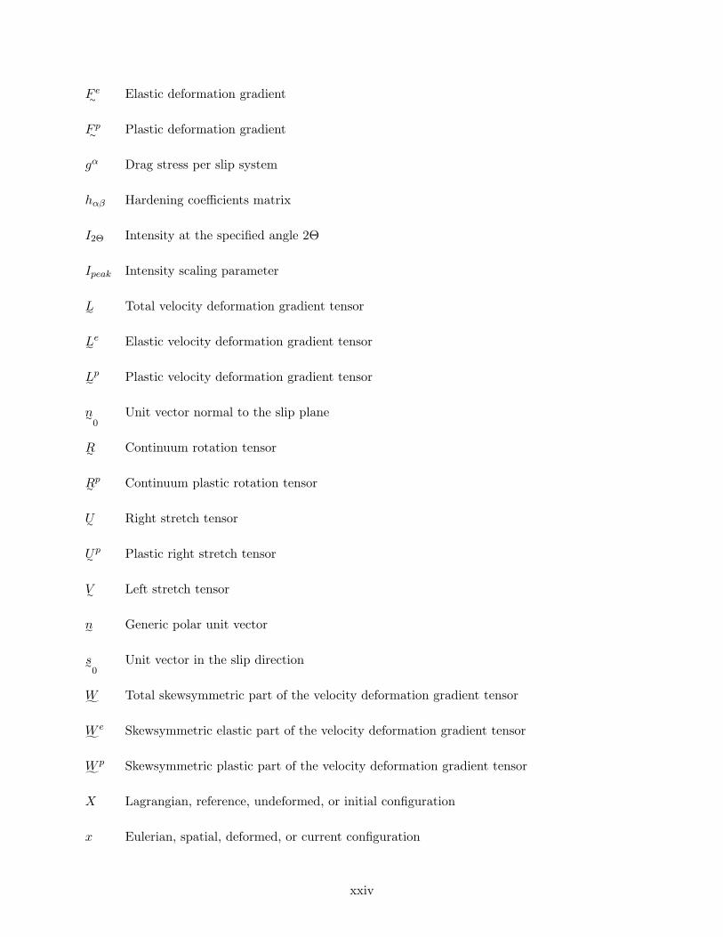
F e∼ Elastic deformation gradient
F p∼ Plastic deformation gradient
gα Drag stress per slip system
hαβ Hardening coefficients matrix
I2Θ Intensity at the specified angle 2Θ
Ipeak Intensity scaling parameter
L˜ Total velocity deformation gradient tensor
L˜e Elastic velocity deformation gradient tensor
L˜p Plastic velocity deformation gradient tensor
n∼0
Unit vector normal to the slip plane
R∼ Continuum rotation tensor
R∼p Continuum plastic rotation tensor
U∼ Right stretch tensor
U∼p Plastic right stretch tensor
V∼ Left stretch tensor
n˜ Generic polar unit vector
s∼0
Unit vector in the slip direction
W˜ Total skewsymmetric part of the velocity deformation gradient tensor
W˜e Skewsymmetric elastic part of the velocity deformation gradient tensor
W˜p Skewsymmetric plastic part of the velocity deformation gradient tensor
X Lagrangian, reference, undeformed, or initial configuration
x Eulerian, spatial, deformed, or current configuration
xxiv
SUMMARY
Gamma-TiAl is an ordered intermetallic compound characterized by high strength to density
ratio, good oxidation resistance, and good creep properties at elevated temperatures. However, it
is intrinsically brittle at room temperature. This thesis investigates the potential for the use of
grinding to process TiAl into useful shapes. Grinding is far from completely understood, and many
aspects of the individual mechanical interactions of the abrasive grit with the material and their
effect on surface integrity are unknown. The development of new synthetic diamond superabrasives
in which shape and size can be controlled raises the question of the influence of those variables on
the surface integrity.
The goal of this work is to better understand the fundamentals of the abrasive grit/material
interaction in grinding operations. Experimental, analytical, and numerical work was done to
characterize and predict the resultant deformation and surface integrity on ground lamellar gamma-
TiAl.
Grinding tests were carried out, by analyzing the effects of grit size and shape, workpiece
speed, wheel depth of cut, and wear on the subsurface plastic deformation depth (PDD). A prac-
tical method to assess the PDD is introduced based on the measurement of the lateral material
flow by 3D non-contact surface profilometry. This method combines the quantitative capabilities
of the microhardness measurement with the sensitivity of Nomarski microscopy. The scope and
limitations of this technique are analyzed. Mechanical properties were obtained by quasi-static and
split Hopkinson bar compression tests. Residual stress plots were obtained by x-ray, and surface
roughness and cracking were evaluated.
The abrasive grit/material interaction was accounted by modeling the force per abrasive grit
for different grinding conditions, and studying its correlation to the PDD. Numerical models of this
interaction were used to analyze boundary conditions, and abrasive size effects on the PDD. An
explicit 2D triple planar slip crystal plasticity model of single point scratching was used to analyze
the effects of lamellae orientation, material anisotropy, and grain boundaries on the deformation.
xxv
CHAPTER I
INTRODUCTION
1.1 Historical Perspective
Grinding is one of the earliest shaping processes known to man. In the Neolithic Period (15000 to
5000 B.C.) it was used to shape stone tools. Grinding is based on the progressive abrasive wear of
the workpiece by a number of hard grits embedded in a matrix. Mechanization of grinding had been
developed by the middle of the 15th century but the first grinding machine was not built until about
1830 (Woodbury, 1959). Early research on grinding was based on empirical knowledge but the need
for precision and speed required by the 20th century’s industry provided the driving force for more
specialized research in the area. During the 1970’s and 1980’s numerous phenomenological models
were developed as shown in Shaw (1972), Hahn and Lindsay (1982a,b,c,d), and Malkin (1989). This
trend faded for several reasons: basic industry needs were met, the work yielded only particular
results, the models needed to be calibrated with extensive, time consuming and expensive tests,
and during the last years cylindrical grinding has been replaced by hard turning. The research
reported in this thesis re-examines grinding as a cost effective technique for shaping intermetallic
compounds, and its implications for surface integrity. Intermetallic compounds refer to a phase type
formed when atoms of two or more metals combine in relatively simple stoichiometric proportions to
produce a crystal different in structure from the individual metals. The constituent elements have
strong bonds, that typically include metallic, ionic or covalent types and are usually ordered in two
or more sublattices, each with its own distinct population of atoms. Intermetallics have long-range
order on their crystal structure below a critical temperature. Deviations from precise stoichiometry
on one or both sides of the nominal ideal atomic ratios produces partial disorder. The relatively high
activation energy for chemical diffusion in the ordered lattice causes high creep resistance at elevated
temperatures. The ordered intermetallic structure is characterized by a high strength to density
ratio, good oxidation resistance, and good creep properties at elevated temperatures. However, this
intrinsically strong atomic bonding is often associated with brittleness at room temperature (Larsen
1
et al., 1996), making the shaping process critical to structural integrity. The interest in γ − TiAl
intermetallic compounds started in the 1950’s motivated by its light weight and its potential for
the kind of high temperature applications such as needed by the aeronautical industry (Kim, 1995;
Dimiduk et al., 1992; Austin et al., 1997). Potential applications in combustion engines include
valves, turbine wheels of exhaust gas turbochargers, connecting rods, and piston pins. The mass
reduction leads to improved fuel economy and higher engine performance due to a considerable
decrease of inertia and friction losses. Grinding of γ − TiAl holds the promise of precision high
performance components free of critical defects at minimum time and cost.
1.2 Gamma-TiAl
Intermetallic TiAl-based alloys are well suited for rotary and reciprocating components in en-
gines under high thermal and mechanical load because of their high-temperature properties (Kim,
1989; Kim and Dimiduk, 1991; Clemens et al., 1999; Clemens and Kestler, 2000; Knippscheer and
Frommeyer, 1999). These properties include low density (' 3.8g/cm3), acceptable yield strength
(400 − 650MPa), high specific stiffness (E/ρ ' 46GPa cm3/gm), and good oxidation resistance
and creep up to 700C, at which limitations might arise from microstructural instabilities (Chat-
terjee et al., 2000) which degrade the creep properties, and from an insufficient oxidation resis-
tance (Brady et al., 1996). From room temperature to 800C the thermal expansion coefficient
ranges from 11.5 10−6K−1 to 12.5 10−6K−1, while the thermal conductivity ranges from 19W/m K
to 43W/m K. These values exhibit sufficient thermal compatibility to other engine materials, such
as steels or Ni-based alloys (Knippscheer and Frommeyer, 1999). These properties make TiAl also
appealing for applications as thin films for structural coatings (Kim et al., 2004).
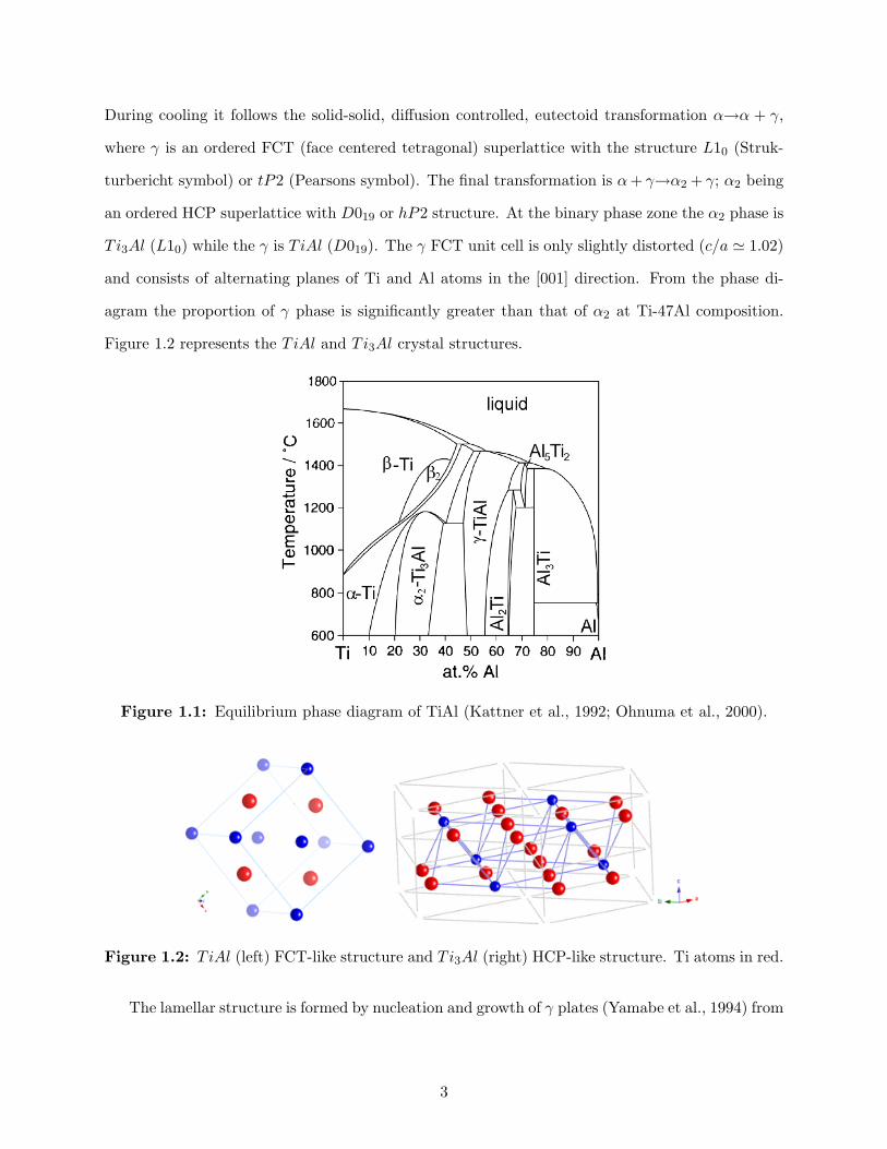
1.2.1 Phase Diagram and Microstructure
Figure 1.1 shows the binary equilibrium phase diagram of Ti-Al (Kattner et al., 1992; Ohnuma
et al., 2000). Most of the research has been focused on the Ti-(45-48)Al (at.%) composition, where
balanced properties of fracture toughness, fatigue life, and tensile strength are achieved. At the
binary composition of Ti-47Al the material begins to solidify partially in the two-phase region
L→L+β, β being a disordered BCC (body centered cubic) phase. The material then goes through
a transformation L + β→L + α, in which α is a disordered HCP (hexagonal closed packed) phase.
2
During cooling it follows the solid-solid, diffusion controlled, eutectoid transformation α→α + γ,
where γ is an ordered FCT (face centered tetragonal) superlattice with the structure L10 (Struk-
turbericht symbol) or tP2 (Pearsons symbol). The final transformation is α + γ→α2 + γ; α2 being
an ordered HCP superlattice with D019 or hP2 structure. At the binary phase zone the α2 phase is
Ti3Al (L10) while the γ is TiAl (D019). The γ FCT unit cell is only slightly distorted (c/a ' 1.02)
and consists of alternating planes of Ti and Al atoms in the [001] direction. From the phase di-
agram the proportion of γ phase is significantly greater than that of α2 at Ti-47Al composition.
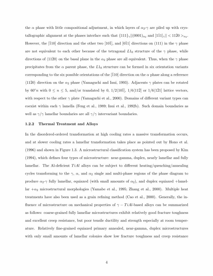
Figure 1.2 represents the TiAl and Ti3Al crystal structures.
Figure 1.1: Equilibrium phase diagram of TiAl (Kattner et al., 1992; Ohnuma et al., 2000).
Figure 1.2: TiAl (left) FCT-like structure and Ti3Al (right) HCP-like structure. Ti atoms in red.
The lamellar structure is formed by nucleation and growth of γ plates (Yamabe et al., 1994) from
3
the α phase with little compositional adjustment, in which layers of α2-γ are piled up with crys-
tallographic alignment at the phases interface such that 111γ ||(0001)α2 and [111]γ || < 1120 >α2 .
However, the [110] direction and the other two [101], and [011] directions on (111) in the γ phase
are not equivalent to each other because of the tetragonal L10 structure of the γ phase, while
directions of 〈1120〉 on the basal plane in the α2 phase are all equivalent. Thus, when the γ phase
precipitates from the α parent phase, the L10 structure can be formed in six orientation variants
corresponding to the six possible orientations of the [110] direction on the α phase along a reference
〈1120〉 direction on the α2 phase (Yamaguchi and Inui, 1993). Adjacents γ plates can be rotated
by 60n with 0 ≤ n ≤ 5, and/or translated by 0, 1/2〈101], 1/6〈112] or 1/6〈121] lattice vectors,
with respect to the other γ plate (Yamaguchi et al., 2000). Domains of different variant types can
coexist within each γ lamella (Feng et al., 1989; Inui et al., 1992b). Such domain boundaries as
well as γ/γ lamellar boundaries are all γ/γ intervariant boundaries.
1.2.2 Thermal Treatment and Alloys
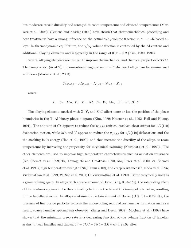
In the disordered-ordered transformation at high cooling rates a massive transformation occurs,
and at slower cooling rates a lamellar transformation takes place as pointed out by Hono et al.
(1996) and shown in Figure 1.3. A microstructural classification system has been proposed by Kim
(1994), which defines four types of microstructure: near-gamma, duplex, nearly lamellar and fully
lamellar. The Al-deficient TiAl alloys can be subject to different heating/quenching/annealing
cycles transforming to the γ, α, and α2 single and multi-phase regions of the phase diagram to
produce α2-γ fully lamellar, equiaxed (with small amounts of α2), and duplex equiaxed +lamel-
lar +α2 microstructural morphologies (Yamabe et al., 1995; Zhang et al., 2000). Multiple heat
treatments have also been used as a grain refining method (Cao et al., 2000). Generally, the in-
fluence of microstructure on mechanical properties of γ − TiAl-based alloys can be summarized
as follows: coarse-grained fully lamellar microstructures exhibit relatively good fracture toughness
and excellent creep resistance, but poor tensile ductility and strength especially at room temper-
ature. Relatively fine-grained equiaxed primary annealed, near-gamma, duplex microstructures
with only small amounts of lamellar colonies show low fracture toughness and creep resistance
4
but moderate tensile ductility and strength at room temperature and elevated temperatures (Mar-
ketz et al., 2003). Clemens and Kestler (2000) have shown that thermomechanical processing and
heat treatments have a strong influence on the actual γ/α2-volume fraction in γ − TiAl-based al-
loys. In thermodynamic equilibrium, the γ/α2 volume fraction is controlled by the Al-content and
additional alloying elements and is typically in the range of 0.05− 0.2 (Kim, 1989, 1994).
Several alloying elements are utilized to improve the mechanical and chemical properties of TiAl.
The composition (in at.%) of conventional engineering γ − TiAl-based alloys can be summarized
as follows (Marketz et al., 2003):
Ti45−52 −Al45−48 −X1−3 − Y2−5 − Z<1
where
X = Cr, Mn, V ; Y = Nb, Ta, W, Mo; Z = Si, B, C
The alloying elements marked with X, Y, and Z all affect more or less the position of the phase
boundaries in the Ti-Al binary phase diagram (Kim, 1989; Kattner et al., 1992; Hall and Huang,
1991). The addition of Cr appears to reduce the τCRSS (critical resolved shear stress) for 1/2〈110]
dislocation motion, while Mn and V appear to reduce the τCRSS for 1/2〈110] dislocations and the
the stacking fault energy (Hao et al., 1999), and thus increase the ductility of the alloys at room
temperature by increasing the propensity for mechanical twinning (Kawabata et al., 1989). The
other elements are used to improve high temperature characteristics such as oxidation resistance
(Nb, Shemet et al. 1999; Ta, Yamaguchi and Umakoshi 1990; Mo, Perez et al. 2000; Zr, Shemet
et al. 1999), high temperature strength (Nb, Tetsui 2002), and creep resistance (Si, Noda et al. 1995;
Viswanathan et al. 1999; W, Seo et al. 2001; C, Viswanathan et al. 1999). Boron is typically used as
a grain refining agent. In alloys with a trace amount of Boron (B ≤ 0.03at.%), the solute drag effect
of Boron atoms appears to be the controlling factor on the lateral thickening of γ lamellae, resulting
in fine lamellar spacing. In alloys containing a certain amount of Boron (B ≥ 0.1− 0.2at.%), the
presence of fine boride particles reduces the undercooling required for lamellar formation and as a
result, coarse lamellar spacing was observed (Zhang and Deevi, 2002). McQuay et al. (1999) have
shown that the minimum creep rate is a decreasing function of the volume fraction of lamellar
grains in near lamellar and duplex Ti− 47Al − 2Nb− 2Mn with TiB2 alloy.
5
Textures play a special role in the γ − TiAl based intermetallic alloys. Under industrial con-
ditions with relatively slow solidification the ingots have a dendritic growth in the direction of
heat flow and a very strong local texture. The lamellae planes 111 are aligned normal to the
solidification direction and are parallel to the cylindrical surfaces of the ingots. Pores and micro-
scopic shrinkage cavities within the as-cast material can be eliminated by an adequate hot isostatic
pressing (HIP) process or thermomechanical treatment.
Figure 1.3: CCT curves showing the solid-solid transformation on Ti-48Al (Hono et al., 1996).
1.2.3 Deformation Mechanisms
The deformation modes of γ − TiAl-based alloys strongly depend on their microstructure, alloy
composition and temperature. The single α2 − Ti3Al phase is more hard and brittle than the
γ − TiAl phase and it has a significant effect on the mechanical properties, deformation behavior
and ductility of γ−TiAl two phase alloys. It is well established (Inui et al., 1992a; Yamaguchi and
Umakoshi, 1990; Appel and Wagner, 1998) that deformation of γ − TiAl under most conditions
occurs on 111 planes by activation of ordinary dislocations with the Burgers vector b = 1/2〈110〉
and superdislocations with the Burgers vector b = 〈101〉 and b = 〈112〉, respectively. In addition
mechanical twinning along 1/6〈112〉111 occurs that does not alter the ordered L10 structure of
the γ−TiAl. Figure 1.5 shows the potential slip and twinning systems of the L10 structure, in the
schematic drawing of a three-layer sequence of atom stacking on the (111) plane. It can be seen
from Fig. 1.5 that along the 〈110〉-directions there is only one type of atom (either Ti or Al). This
type of dislocation is called ordinary dislocation, and referred to as “easy slip”. By contrast Ti-
atoms and Al-atoms interchange in 〈011〉-directions and, therefore, the so-called superdislocations
6
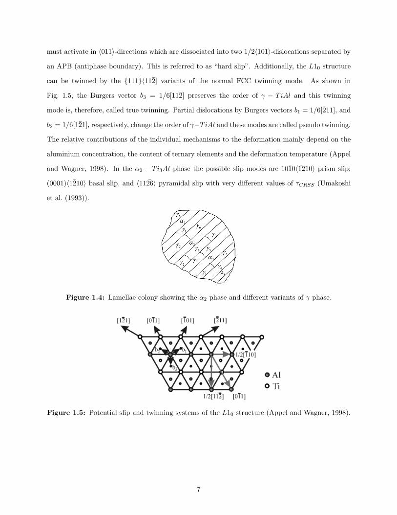
must activate in 〈011〉-directions which are dissociated into two 1/2〈101〉-dislocations separated by
an APB (antiphase boundary). This is referred to as “hard slip”. Additionally, the L10 structure
can be twinned by the 111〈112] variants of the normal FCC twinning mode. As shown in
Fig. 1.5, the Burgers vector b3 = 1/6[112] preserves the order of γ − TiAl and this twinning
mode is, therefore, called true twinning. Partial dislocations by Burgers vectors b1 = 1/6[211], and
b2 = 1/6[121], respectively, change the order of γ−TiAl and these modes are called pseudo twinning.
The relative contributions of the individual mechanisms to the deformation mainly depend on the
aluminium concentration, the content of ternary elements and the deformation temperature (Appel
and Wagner, 1998). In the α2 − Ti3Al phase the possible slip modes are 1010〈1210〉 prism slip;
(0001)〈1210〉 basal slip, and 〈1126〉 pyramidal slip with very different values of τCRSS (Umakoshi
et al. (1993)).
Figure 1.4: Lamellae colony showing the α2 phase and different variants of γ phase.
Figure 1.5: Potential slip and twinning systems of the L10 structure (Appel and Wagner, 1998).
7
1.3 Grinding
Grinding is a material removal process that is used to achieve fine surface finishes, tight geometric
tolerances, and complex contours. Grinding is a multipoint machining process with a stochastic
distribution of tool geometries like grain size, rake (attack) angle, etc., producing a distribution on
process parameters such as grit force, grit depth of cut, among others. Due to the negative rake
angle of the grinding wheel abrasive grits, the specific cutting energy (energy consumed to remove
a unit volume of material) of this process is higher than in other machining processes like turning,
milling, etc. (Wang and Subhash, 2002). Consequently the material is subjected to high plastic
deformation and temperature gradients. There are four primary types of grinding according to the
workpiece desired geometry: surface, cylindrical, internal, and centerless grinding (Tlusty, 1999).
Although surface grinding is the focus of this research the results can be utilized for other grinding
operations. Also, grinding can be categorized according to the DoC, as creep-feed grinding used
for stock removal where the DoC is of the order of several millimeters; and finish grinding where
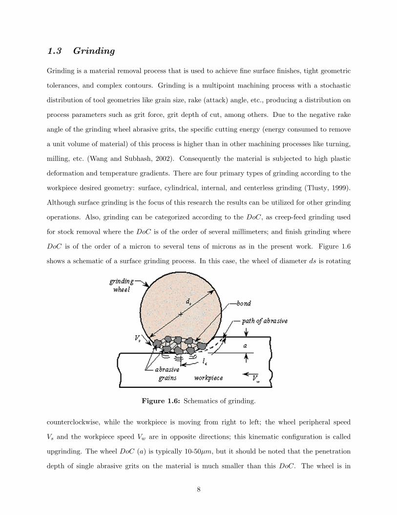
DoC is of the order of a micron to several tens of microns as in the present work. Figure 1.6
shows a schematic of a surface grinding process. In this case, the wheel of diameter ds is rotating
Figure 1.6: Schematics of grinding.
counterclockwise, while the workpiece is moving from right to left; the wheel peripheral speed
Vs and the workpiece speed Vw are in opposite directions; this kinematic configuration is called
upgrinding. The wheel DoC (a) is typically 10-50µm, but it should be noted that the penetration
depth of single abrasive grits on the material is much smaller than this DoC. The wheel is in
8
contact with the workpiece along the contact length lc, in a width b, perpendicular to the page and
parallel to the axis of rotation. Conventional grinding uses Al2O3 (aluminum oxide), and SiC (silicon
carbide), and with the industrial production of synthetic superabrasive particles, CBN (cubic boron
nitride) and diamond have come into current use. These superabrasives are considerably harder
than conventional abrasives allowing the machining of hard materials while presenting less wear.
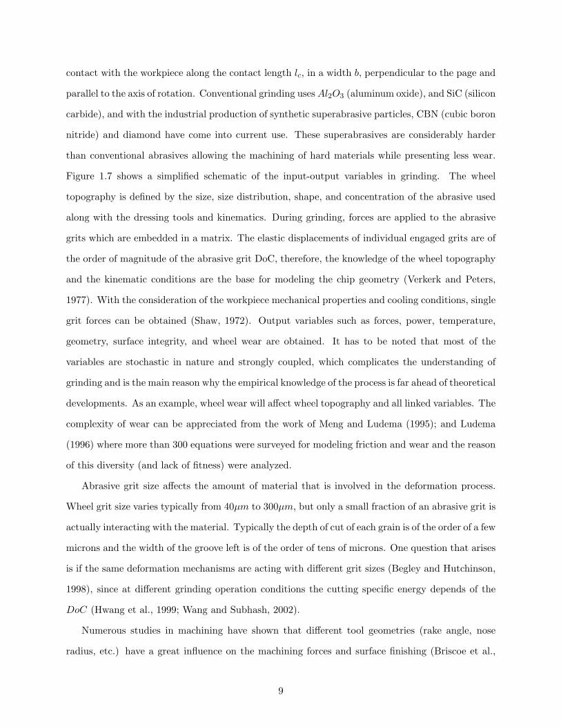
Figure 1.7 shows a simplified schematic of the input-output variables in grinding. The wheel
topography is defined by the size, size distribution, shape, and concentration of the abrasive used
along with the dressing tools and kinematics. During grinding, forces are applied to the abrasive
grits which are embedded in a matrix. The elastic displacements of individual engaged grits are of
the order of magnitude of the abrasive grit DoC, therefore, the knowledge of the wheel topography
and the kinematic conditions are the base for modeling the chip geometry (Verkerk and Peters,
1977). With the consideration of the workpiece mechanical properties and cooling conditions, single
grit forces can be obtained (Shaw, 1972). Output variables such as forces, power, temperature,
geometry, surface integrity, and wheel wear are obtained. It has to be noted that most of the
variables are stochastic in nature and strongly coupled, which complicates the understanding of
grinding and is the main reason why the empirical knowledge of the process is far ahead of theoretical
developments. As an example, wheel wear will affect wheel topography and all linked variables. The
complexity of wear can be appreciated from the work of Meng and Ludema (1995); and Ludema
(1996) where more than 300 equations were surveyed for modeling friction and wear and the reason
of this diversity (and lack of fitness) were analyzed.
Abrasive grit size affects the amount of material that is involved in the deformation process.
Wheel grit size varies typically from 40µm to 300µm, but only a small fraction of an abrasive grit is
actually interacting with the material. Typically the depth of cut of each grain is of the order of a few
microns and the width of the groove left is of the order of tens of microns. One question that arises
is if the same deformation mechanisms are acting with different grit sizes (Begley and Hutchinson,
1998), since at different grinding operation conditions the cutting specific energy depends of the
DoC (Hwang et al., 1999; Wang and Subhash, 2002).
Numerous studies in machining have shown that different tool geometries (rake angle, nose
radius, etc.) have a great influence on the machining forces and surface finishing (Briscoe et al.,
9
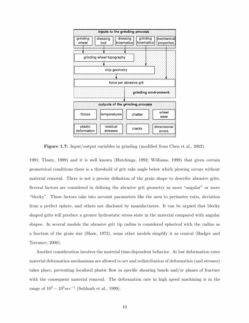
Figure 1.7: Input/output variables in grinding (modified from Chen et al., 2002).
1991; Tlusty, 1999) and it is well known (Hutchings, 1992; Williams, 1999) that given certain
geometrical conditions there is a threshold of grit rake angle below which plowing occurs without
material removal. There is not a precise definition of the grain shape to describe abrasive grits.
Several factors are considered in defining the abrasive grit geometry as more “angular” or more
“blocky”. These factors take into account parameters like the area to perimeter ratio, deviation
from a perfect sphere, and others not disclosed by manufacturers. It can be argued that blocky
shaped grits will produce a greater hydrostatic stress state in the material compared with angular
shapes. In several models the abrasive grit tip radius is considered spherical with the radius as
a fraction of the grain size (Shaw, 1972), some other models simplify it as conical (Badger and
Torrance, 2000).
Another consideration involves the material time-dependent behavior. At low deformation rates
material deformation mechanisms are allowed to act and redistribution of deformation (and stresses)
takes place, preventing localized plastic flow in specific shearing bands and/or planes of fracture
with the consequent material removal. The deformation rate in high speed machining is in the
range of 103 − 105sec−1 (Subhash et al., 1999).
10
1.4 Effects of Machining on Gamma-TiAl
Machining processes can have an effect on the mechanical properties of the workpiece, in particular
they can impact the high cycle fatigue (HCF) performance which is different from the one predicted
using polished samples (Trail and Bowen, 1995; Bentley et al., 1999; Jones and Eylon, 1999; Sharman
et al., 2001b; Novovic et al., 2004), and tensile properties (Schneibel et al., 1993; Darolia and
Walston, 1996). These effects can be positive in incrementing the HCF life by leaving a surface
layer with compressive residual stress (Balart et al., 2004) or recrystallized material of smaller
grain size compared to the parent (Jones and Eylon, 1999); but detrimental effects are more often
observed due to generation of cracks or tensile residual stress.
The high energy input during grinding creates a temperature gradient with the consequent
thermal deformation gradient and the possibility of generating tensile residual stresses (Mahdi and
Zhang, 1997), cracking (Eda et al., 1983), and dimensional instabilities (Kagiwada and Kanauchi,
1985). Also, the material thermomechanical history has to be considered. As grinding is a multipass
process, subsurface material layers are subjected to thermal and mechanical deformation cycles.
Also, it is important to consider that plastic deformation and damage are cumulative in the material
where usually no healing processes take place during machining. Therefore low cycle fatigue may
be the cause of fracture in some brittle intermetallic compounds or ceramics during grinding.
Residual stresses (RS) in grinding can originate from a contribution of thermomechanical ef-
fects that produce inhomogeneous deformation. Some causes are the scratching of abrasive grits,
cumulative deformation leading to fracture, thermally-induced deformation, or due to phase trans-
formations in which there is a volume change (Mahdi and Zhang, 1997). Grinding operating
conditions can leave either compressive, in what was called “gentle grinding conditions” or tensile
residual stresses in “abusive grinding conditions” as shown in Fig. 1.8 by the early work of Field
(1972). During grinding thermal effects become important when material properties are sensitive
to temperature, where phase transformations or thermal cracking may take place (Grum, 2001).
Thermally activated mechanisms will be favored, with eventual changes of the material behav-
ior (i.e. brittle/ductile transition, dislocation annihilation, etc). The compressive/tensile residual
stress transition is due in part to thermal effects as shown by Balart et al. (2004), who have found
that a material dependent critical surface temperature has to be reached to left tensile residual
11
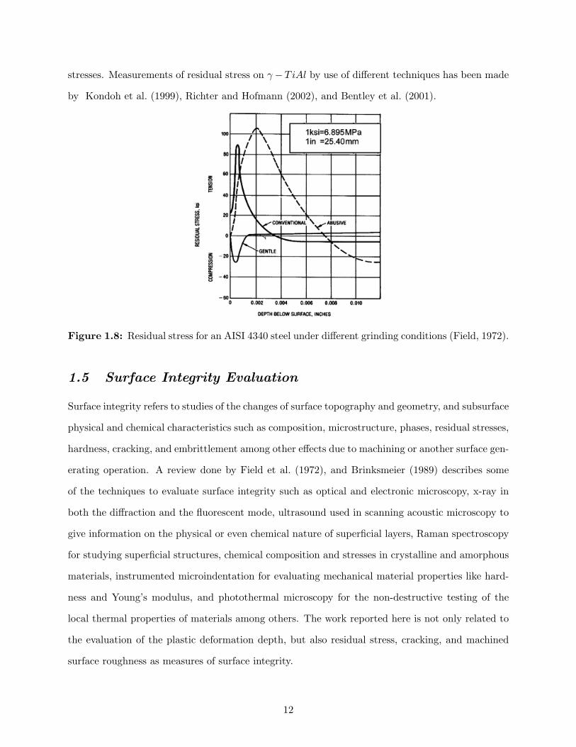
stresses. Measurements of residual stress on γ−TiAl by use of different techniques has been made
by Kondoh et al. (1999), Richter and Hofmann (2002), and Bentley et al. (2001).
Figure 1.8: Residual stress for an AISI 4340 steel under different grinding conditions (Field, 1972).
1.5 Surface Integrity Evaluation
Surface integrity refers to studies of the changes of surface topography and geometry, and subsurface
physical and chemical characteristics such as composition, microstructure, phases, residual stresses,
hardness, cracking, and embrittlement among other effects due to machining or another surface gen-
erating operation. A review done by Field et al. (1972), and Brinksmeier (1989) describes some
of the techniques to evaluate surface integrity such as optical and electronic microscopy, x-ray in
both the diffraction and the fluorescent mode, ultrasound used in scanning acoustic microscopy to
give information on the physical or even chemical nature of superficial layers, Raman spectroscopy
for studying superficial structures, chemical composition and stresses in crystalline and amorphous
materials, instrumented microindentation for evaluating mechanical material properties like hard-
ness and Young’s modulus, and photothermal microscopy for the non-destructive testing of the
local thermal properties of materials among others. The work reported here is not only related to
the evaluation of the plastic deformation depth, but also residual stress, cracking, and machined
surface roughness as measures of surface integrity.
12
1.5.1 Plastic Deformation Depth Measurement
Measurement of hardness due to cold work in the subsurface is one of the most widespread methods
for determining deformed zones. These measurements are usually represented as plots of hardness
versus depth taking as a base line the bulk hardness such as shown in the work of Field et al. (1972);
Bentley et al. (1999); Jones and Eylon (1999). The size of the hardened zone is of the order of tens to
hundred of microns, and microhardness techniques need to be used in order to measure the hardness
gradient. Some techniques are the micro-Vickers, Knoop, and Berkovich, whose description can be
found somewhere else, for example in Newby (1989). Scratching is a derivation of the microhardness
technique, and it consists of scratching the material with a given force and then measuring the
scratched groove width as a function of distance to the edge. Simple models can be applied to
determine the hardening (Liu et al., 2002). A disadvantage of this technique is the scatter that
usually accompanies the results. This scatter is due to uncertainties in measurement of the indent
diagonals, and in the case of γ − TiAl, its anisotropic mechanical behavior, and heterogeneity of
properties between the α2 and γ phases, that distorts the indent geometry. Another disadvantage
is that microhardness cannot be measured close to deformed edges, not only because of lack of
surrounding material, but also because the lack of surface planarity impairs indentation.
Optical microscopy is another technique to evaluate PDD (plastic deformation depth) and it
is based on the observation of ridges at surfaces. It usually uses Nomarski illumination which is
especially suited for the evaluation of surface quality and defects that otherwise with regular mi-
croscopy/SEM would not be visible (see Robinson and Bradbury, 1992). The Nomarski illumination
method incorporates polarization and phase shift techniques that cause minute departures of the
surface from a perfect plane to appear as different colors. All quantitative measurements are made
by using a reticule in the optics objective. As with any observational technique the disadvantage
is that it is subjective.
Xu and Jahanmir (1994) developed the bonded interface, or split specimen technique, to observe
damage on machined ceramics using Nomarski microscopy. Damage was defined in their work as
the presence of cracks, and/or twins, and/or slip bands. In their technique two polished surfaces
of the (split) sample are glued together with cyanoacrylate (super glue), the specimen is machined
and the two surfaces are separated and placed under the microscope.
13
Nelson (1997) utilized the bonded interface technique to observe the PDD on ground TiAl
samples and further implemented the use of a profilometer to evaluate the damaged zone by changes
in the surface roughness. Under conditions of plastic deformation, twins/shear bands will produce
some roughness on the polished surfaces of the sample. Razavi (2000), and later Stone (2003) had
used the same technique for measuring PDD in their work. The disadvantage of this technique
lies in the difficulty of surface sample preparation, and the resulting variable spacing of the glued
interfaces in the sample and, between samples, that leads to a large variability of results due to
variable mechanical constraint conditions.
14
CHAPTER II
PRESENT WORK
2.1 Motivation
Grinding of γ − TiAl is far from completely understood, and many aspects of the individual me-
chanical interactions of the abrasive grit with the material and their effect on surface integrity are
unknown.
Data on machinability, surface integrity, and fatigue performance of γ−TiAl-based alloys have
been published by researchers at The University of Birmingham (Trail and Bowen, 1995; Bentley
et al., 1999, 2001; Sharman et al., 2001a,b; Mantle and Aspinwall, 2001; Novovic et al., 2004). They
have carried out hardness profiling, 2D surface roughness parameters determination, microscopy
cracking evaluation, and in some cases residual stress measurements by using the hole drilling
method and strain gages. All the experimental data were analyzed statistically with the operation
parameters and their conclusions based on that analysis.
Jones (1997); Jones and Eylon (1999) have worked on the fatigue resistance of machined TiAl
at RT on samples with and without heat treatment after machining. After a comprehensive fracto-
graphic analysis and microstructure evaluation, they concluded that the fatigue life is affected by
machining conditions and that at high temperatures the fatigue crack initiation site changes from
surface to bulk. They have observed that a recrystallized zone of smaller grain size is formed on
machined surfaces after they were heat treated at 750C for 1hr. Surface integrity was evaluated
with the Nomarski microscopy and hardness profiling. Machining parameters were not explic-
itly considered nor was a model proposed for the relation of these parameters with the observed
behavior.
The work performed at The Georgia Institute of Technology by Nelson (1997); Razavi (2000);
and Stone (2003) has been based on the use of the split-sample technique and 2D profilometry to
measure subsurface damage, and the use of the model of Lawn and Wilshaw (1975) and Aurora et al.
(1979) to relate the total grinding normal force with the damage. Even though the model of Lawn
15
and Wilshaw (1975) and Aurora et al. (1979) relates the indentation force, material hardness and
indenter geometry to the PDD for a single indenter, Nelson (1997); Razavi (2000); and Stone
(2003) related the total normal force in grinding with the PDD without considering the indentation
process itself. Furthermore, the technique utilized for PDD determination was dependent on the
user’s experimental skills in sample preparation, selection of the site to measure the profile, and
criteria to separate the deformed from the undeformed zone.
The individual mechanical interactions of the abrasive grit in grinding differs from material to
material. Models for PDD prediction should account for the interaction of single abrasive grits
with the material to have some physical insight of the process. This interaction is produced at
the microscopic length scale, and material dependent deformation mechanisms at that scale level
should be accounted for. In the present case those are individual lamellae colonies presenting elastic
and viscoplastic anisotropy, grain boundaries and their effect on local deformation behavior that
can yield to localized failures, and relative abrasive grit/lamellae size effects that will also influence
strain localization and failure.
There is also the need to develop a validated and systematic experimental technique to obtain
information which could be related to mechanical performance, in particular to HCF. As reported
by Jones (1997); Jones and Eylon (1999), the technique of microhardness evaluation is not as
sensitive as the Nomarski microscopy to define the PDD because of measurement uncertainties.
The development of new synthetic superabrasives in which shape and size can be controlled
raises the question of the influence those variables may have on surface integrity since it can be
argued that blocky shaped grits will produce a greater hydrostatic stress state than angular grits.
The progress on testing instrumentation, and specifically the advent of 3D non-contact surface
profilometry (Forman, 1979) allows to perform quantitative evaluation of deformed surfaces. Ver-
tical resolution of the order of nanometers can be easily achieved and the possibility of analyzing
relatively large areas (of several mm2) with resolution of the order of microns allows the study of
quantitative deformation inhomogeneity i.e. due to grain size effects. The advance in numerical
computer software along with computer power allows huge amounts of experimental data to be
analyzed in a reasonable time.
The recent advances in crystal plasticity models of γ − TiAl, along with the improvement on
16
the kinematics of grinding modeling, present the opportunity to relate the macroscopic grinding
variables to the individual grit forces and better understand the fundamentals of the interaction
between individual abrasive grits and individual lamellar colonies.
2.2 Objective
To better understand the fundamentals of the abrasive grit/material interaction in grinding oper-
ations, and resultant deformation and surface integrity on lamellar γ − TiAl.
2.3 Methodology and Outline
The present work contains experimental, analytical, and numerical developments as shown in the
overview of Fig. 2.1. In the experimental part of the work, Chapter 3 presents the chemical, mi-
crostructural and mechanical properties of the present alloy either found in the literature (elastic
constants) or obtained through dynamic, and quasi-static compression tests and instrumented in-
dentation. Chapter 4 presents the detailed experimental technique developed for the evaluation
of the PDD based on the works of Xu and Jahanmir (1994); and Nelson (1997), with the range
of applicability and limitations. Chapter 5 presents the grinding experimental methodology and
statistical analysis of results, including PDD, surface parameters, and cracking. Appendix A com-
pletes the chapter with the table of the complete set of grinding experimental data. Chapter 6
presents the methodology utilized to measure and analyze RS on the surface and subsurface of
selected ground samples, based on the work of Winholtz and Cohen (1988); Wagner et al. (1983);
and Richter and Hofmann (2002), as well as the RS data analysis. Appendix B completes the
chapter with the data obtained by analysis as well as experimental vs. analytical comparison plots
of strain. Chapter 7 presents the modeling of the force per abrasive grit for different grinding con-
ditions based on the work of Hecker (2002). The analysis of the correlation of this parameter with
PDD is also presented. Chapter 8 presents the two numerical models used to simulate indentation
and scratching of abrasive grits on the material. One model utilizes isotropic elastic-viscoplastic
properties and it is utilized to obtain the difference in PDD under PE (plane strain) and PS (plane
stress) conditions of indentation and relate the PDD measured at the sample free surface with the
one at the material bulk. 3D scratching models were utilized to analyze the variation of PDD
17
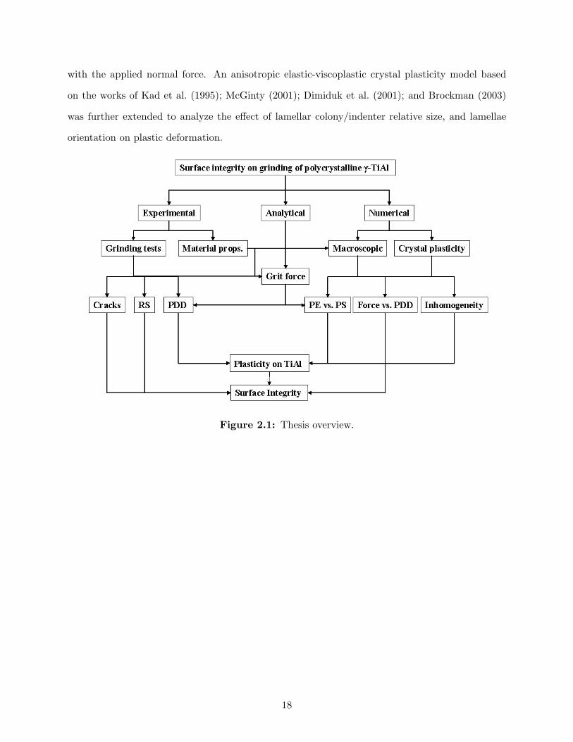
with the applied normal force. An anisotropic elastic-viscoplastic crystal plasticity model based
on the works of Kad et al. (1995); McGinty (2001); Dimiduk et al. (2001); and Brockman (2003)
was further extended to analyze the effect of lamellar colony/indenter relative size, and lamellae
orientation on plastic deformation.
Figure 2.1: Thesis overview.
18

CHAPTER III
MATERIAL CHARACTERIZATION
This Chapter presents the metallurgical and mechanical material characterization section that was
needed for input into the numerical models. Chemical composition and microstructure were an-
alyzed, and the elastic constants of individual phases, and lamellae obtained from the literature.
Dynamic and quasi-static compression tests as well as instrumented indentation tests were per-
formed at RT.
3.1 Chemical Composition and Metallography
The alloy used for this research was Howmet’s 47XD Titanium Aluminide with a composition of
Ti-47Al-2Nb-2Mn-0.3B at. %, produced by induction skull melting into slabs of 25mm thickness.
In order to reduce porosity and homogenize the microstructure, the slabs were HIPped at 1300C
at 165MPa for 4hs with a subsequent heat treatment at 1010C for 50hs. Figure 3.1 shows the
phase diagram of Ti-Al indicating the different phase crystal structure. TiAl-based alloys with
slightly Al-deficient compositions exhibit γ/α2 microstructures and often contain a considerable
volume fraction of morphologically lamellar colonies as in the present case. The lamellar colonies
consist of a majority of variants of γ-TiAl and α2-Ti3Al lamellae. The addition of Mn improves the
RT ductility (Kawabata et al., 1989; Hao et al., 1999); the addition of Nb improves the oxidation
resistance (Shemet et al., 1999), and high temperature strength (Tetsui, 2002), the addition of
Boron is used for grain refinement (Zhang and Deevi, 2002), and improved creep resistance (McQuay
et al., 1999). Figure 3.2 shows the microstructure of the material used where lamellae colonies of
250µm average size can be observed, while Fig. 3.3 shows a lamellae boundary, where the different
orientation of adjacent colonies can be observed.
19
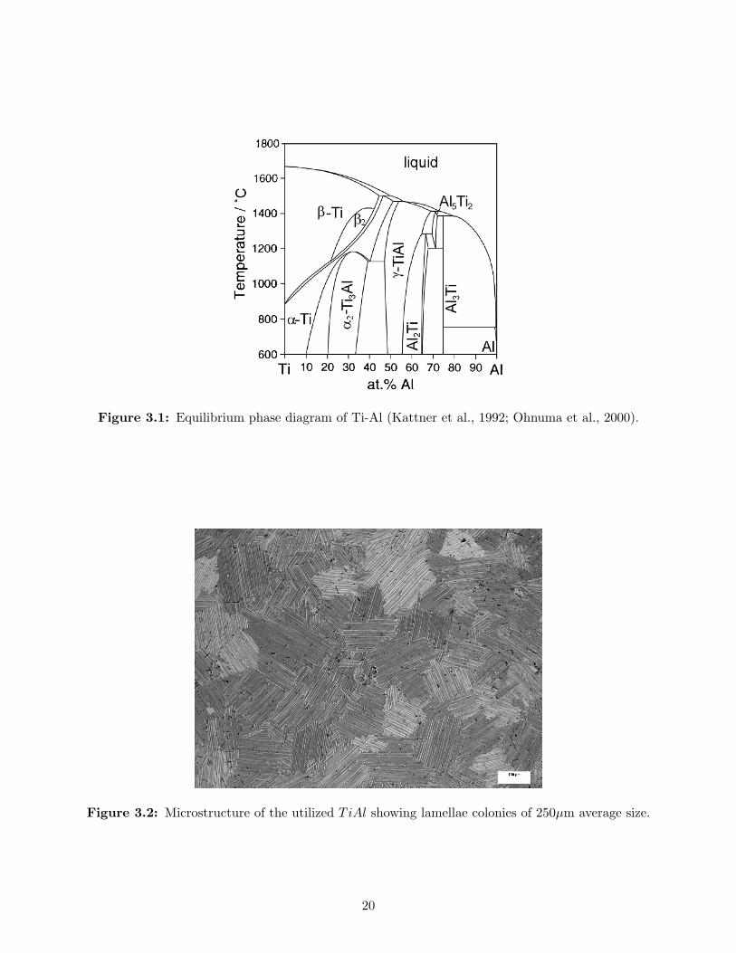
Figure 3.1: Equilibrium phase diagram of Ti-Al (Kattner et al., 1992; Ohnuma et al., 2000).
Figure 3.2: Microstructure of the utilized TiAl showing lamellae colonies of 250µm average size.
20
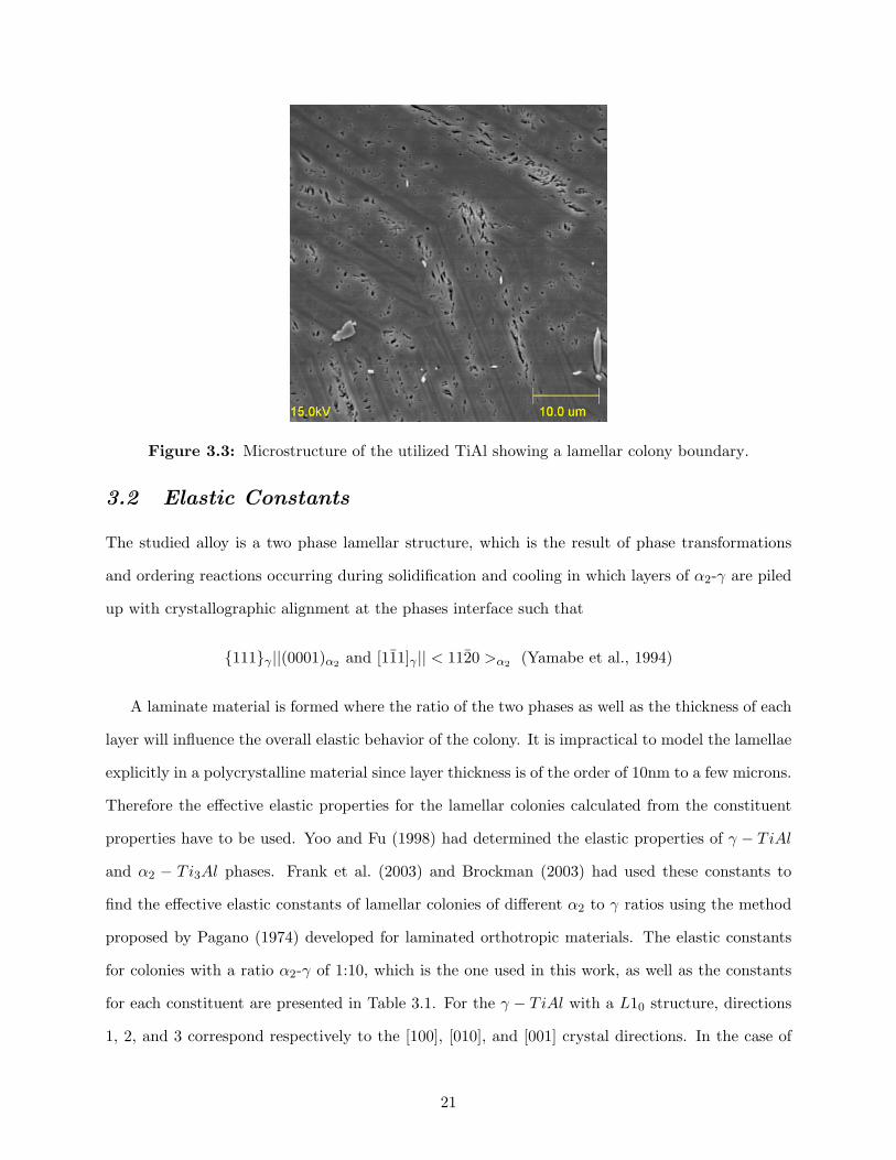
Figure 3.3: Microstructure of the utilized TiAl showing a lamellar colony boundary.
3.2 Elastic Constants
The studied alloy is a two phase lamellar structure, which is the result of phase transformations
and ordering reactions occurring during solidification and cooling in which layers of α2-γ are piled
up with crystallographic alignment at the phases interface such that
111γ ||(0001)α2 and [111]γ || < 1120 >α2 (Yamabe et al., 1994)
A laminate material is formed where the ratio of the two phases as well as the thickness of each
layer will influence the overall elastic behavior of the colony. It is impractical to model the lamellae
explicitly in a polycrystalline material since layer thickness is of the order of 10nm to a few microns.
Therefore the effective elastic properties for the lamellar colonies calculated from the constituent
properties have to be used. Yoo and Fu (1998) had determined the elastic properties of γ − TiAl
and α2 − Ti3Al phases. Frank et al. (2003) and Brockman (2003) had used these constants to
find the effective elastic constants of lamellar colonies of different α2 to γ ratios using the method
proposed by Pagano (1974) developed for laminated orthotropic materials. The elastic constants
for colonies with a ratio α2-γ of 1:10, which is the one used in this work, as well as the constants
for each constituent are presented in Table 3.1. For the γ − TiAl with a L10 structure, directions
1, 2, and 3 correspond respectively to the [100], [010], and [001] crystal directions. In the case of
21
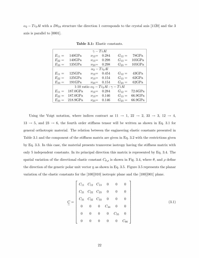
α2 − Ti3Al with a D019 structure the direction 1 corresponds to the crystal axis [1120] and the 3
axis is parallel to [0001].
Table 3.1: Elastic constants.
γ − TiAlE11 = 140GPa ν12= 0.284 G12 = 78GPaE22 = 140GPa ν13= 0.298 G13 = 105GPaE33 = 135GPa ν23= 0.298 G23 = 105GPa
α2 − Ti3AlE11 = 125GPa ν12= 0.454 G12 = 43GPaE22 = 125GPa ν13= 0.154 G13 = 62GPaE33 = 191GPa ν23= 0.154 G23 = 62GPa
1:10 ratio α2 − Ti3Al : γ − TiAlE11 = 187.0GPa ν12= 0.284 G12 = 72.6GPaE22 = 187.0GPa ν13= 0.146 G13 = 66.9GPaE33 = 218.9GPa ν23= 0.146 G23 = 66.9GPa
Using the Voigt notation, where indices contract as 11 → 1, 22 → 2, 33 → 3, 12 → 4,
13 → 5, and 23 → 6, the fourth order stiffness tensor will be written as shown in Eq. 3.1 for
general orthotropic material. The relation between the engineering elastic constants presented in
Table 3.1 and the component of the stiffness matrix are given in Eq. 3.2 with the restrictions given
by Eq. 3.3. In this case, the material presents transverse isotropy having the stiffness matrix with
only 5 independent constants. In its principal direction this matrix is represented by Eq. 3.4. The
spatial variation of the directional elastic constant Cθ,ρ is shown in Fig. 3.4, where θ, and ρ define
the direction of the generic polar unit vector n˜ as shown in Eq. 3.5. Figure 3.5 represents the planar
variation of the elastic constants for the [100][010] isotropic plane and the [100][001] plane.
C˜ =
C11 C12 C13 0 0 0
C21 C22 C23 0 0 0
C31 C32 C33 0 0 0
0 0 0 C44 0 0
0 0 0 0 C55 0
0 0 0 0 0 C66
(3.1)
22
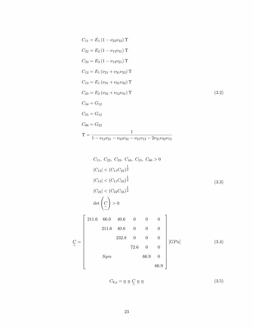
C11 = E1 (1− ν23ν32) Υ
C22 = E2 (1− ν13ν31) Υ
C33 = E3 (1− ν12ν21) Υ
C12 = E1 (ν21 + ν31ν23) Υ
C13 = E1 (ν31 + ν21ν32) Υ
C23 = E2 (ν32 + ν12ν31) Υ
C44 = G12
C55 = G13
C66 = G23
Υ =1
1− ν12ν21 − ν23ν32 − ν31ν13 − 2ν21ν32ν13
(3.2)
C11, C22, C33, C44, C55, C66 > 0
|C12| < (C11C22)12
|C13| < (C11C33)12
|C23| < (C22C33)12
det
(C˜)
> 0
(3.3)
C˜ =
211.6 66.0 40.6 0 0 0
211.6 40.6 0 0 0
232.8 0 0 0
72.6 0 0
Sym 66.9 0
66.9
[GPa] (3.4)
Cθ,ρ = n˜ n˜ C˜ n˜ n˜ (3.5)
23
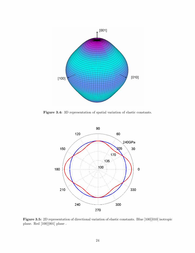
Figure 3.4: 3D representation of spatial variation of elastic constants.
Figure 3.5: 2D representation of directional variation of elastic constants. Blue [100][010] isotropicplane. Red [100][001] plane .
24
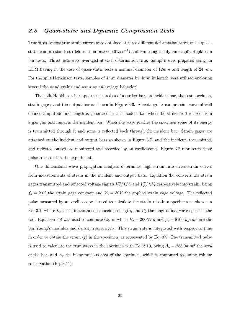
3.3 Quasi-static and Dynamic Compression Tests
True stress versus true strain curves were obtained at three different deformation rates, one a quasi-
static compression test (deformation rate ' 0.01sec−1) and two using the dynamic split Hopkinson
bar tests. Three tests were averaged at each deformation rate. Samples were prepared using an
EDM having in the case of quasi-static tests a nominal diameter of 12mm and length of 24mm.
For the split Hopkinson tests, samples of 4mm diameter by 4mm in length were utilized enclosing
several thousand grains and assuring an average behavior.
The split Hopkinson bar apparatus consists of a striker bar, an incident bar, the test specimen,
strain gages, and the output bar as shown in Figure 3.6. A rectangular compression wave of well
defined amplitude and length is generated in the incident bar when the striker rod is fired from
a gas gun and impacts the incident bar. When the wave reaches the specimen some of its energy
is transmitted through it and some is reflected back through the incident bar. Strain gages are
attached on the incident and output bars as shown in Figure 3.7, and the incident, transmitted,
and reflected pulses are monitored and recorded by an oscilloscope. Figure 3.8 represents these
pulses recorded in the experiment.
One dimensional wave propagation analysis determines high strain rate stress-strain curves
from measurements of strain in the incident and output bars. Equation 3.6 converts the strain
gages transmitted and reflected voltage signals V gT /fsVe and V g
R/fsVe respectively into strain, being
fs = 2.02 the strain gage constant and Ve = 30V the applied strain gage voltage. The reflected
pulse measured by an oscilloscope is used to calculate the strain rate in a specimen as shown in
Eq. 3.7, where Ls is the instantaneous specimen length, and C0 the longitudinal wave speed in the
rod. Equation 3.8 was used to compute C0, in which Eb = 200GPa and ρb = 8100 kg/m3 are the
bar Young’s modulus and density respectively. This strain rate is integrated with respect to time
in order to obtain the strain (ε) in the specimen, as represented by Eq. 3.9. The transmitted pulse
is used to calculate the true stress in the specimen with Eq. 3.10, being Ab = 285.0mm2 the area
of the bar, and As the instantaneous area of the specimen, which is computed assuming volume
conservation (Eq. 3.11).
25
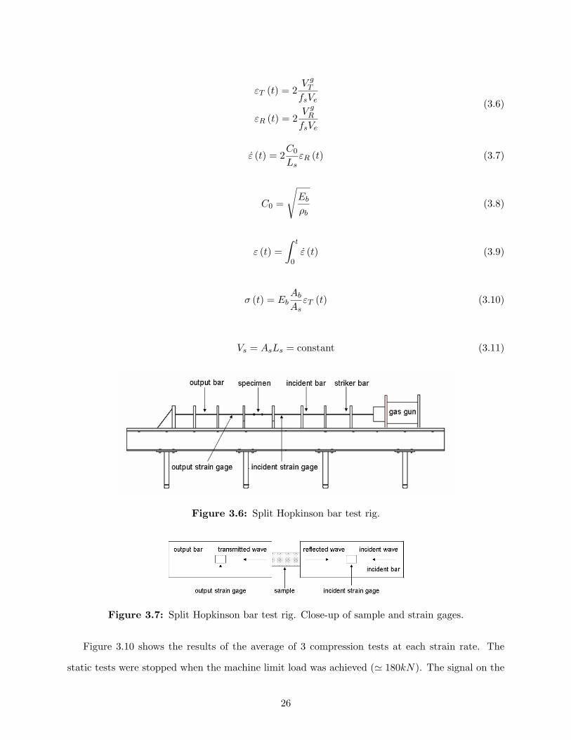
εT (t) = 2V g
T
fsVe
εR (t) = 2V g
R
fsVe
(3.6)
ε (t) = 2C0
LsεR (t) (3.7)
C0 =
√Eb
ρb(3.8)
ε (t) =∫ t
0ε (t) (3.9)
σ (t) = EbAb
AsεT (t) (3.10)
Vs = AsLs = constant (3.11)
Figure 3.6: Split Hopkinson bar test rig.
Figure 3.7: Split Hopkinson bar test rig. Close-up of sample and strain gages.
Figure 3.10 shows the results of the average of 3 compression tests at each strain rate. The
static tests were stopped when the machine limit load was achieved (' 180kN). The signal on the
26
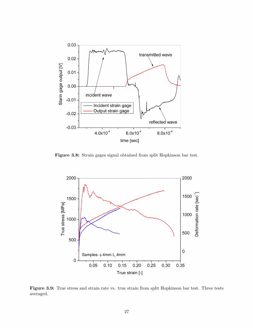
Figure 3.8: Strain gages signal obtained from split Hopkinson bar test.
Figure 3.9: True stress and strain rate vs. true strain from split Hopkinson bar test. Three testsaveraged.
27
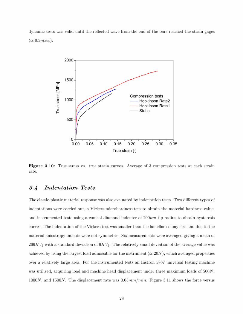
dynamic tests was valid until the reflected wave from the end of the bars reached the strain gages
(' 0.3msec).
Figure 3.10: True stress vs. true strain curves. Average of 3 compression tests at each strainrate.
3.4 Indentation Tests
The elastic-plastic material response was also evaluated by indentation tests. Two different types of
indentations were carried out, a Vickers microhardness test to obtain the material hardness value,
and instrumented tests using a conical diamond indenter of 200µm tip radius to obtain hysteresis
curves. The indentation of the Vickers test was smaller than the lamellae colony size and due to the
material anisotropy indents were not symmetric. Six measurements were averaged giving a mean of
266HV2 with a standard deviation of 6HV2. The relatively small deviation of the average value was
achieved by using the largest load admissible for the instrument (' 20N), which averaged properties
over a relatively large area. For the instrumented tests an Instron 5867 universal testing machine
was utilized, acquiring load and machine head displacement under three maximum loads of 500N ,
1000N , and 1500N . The displacement rate was 0.05mm/min. Figure 3.11 shows the force versus
28
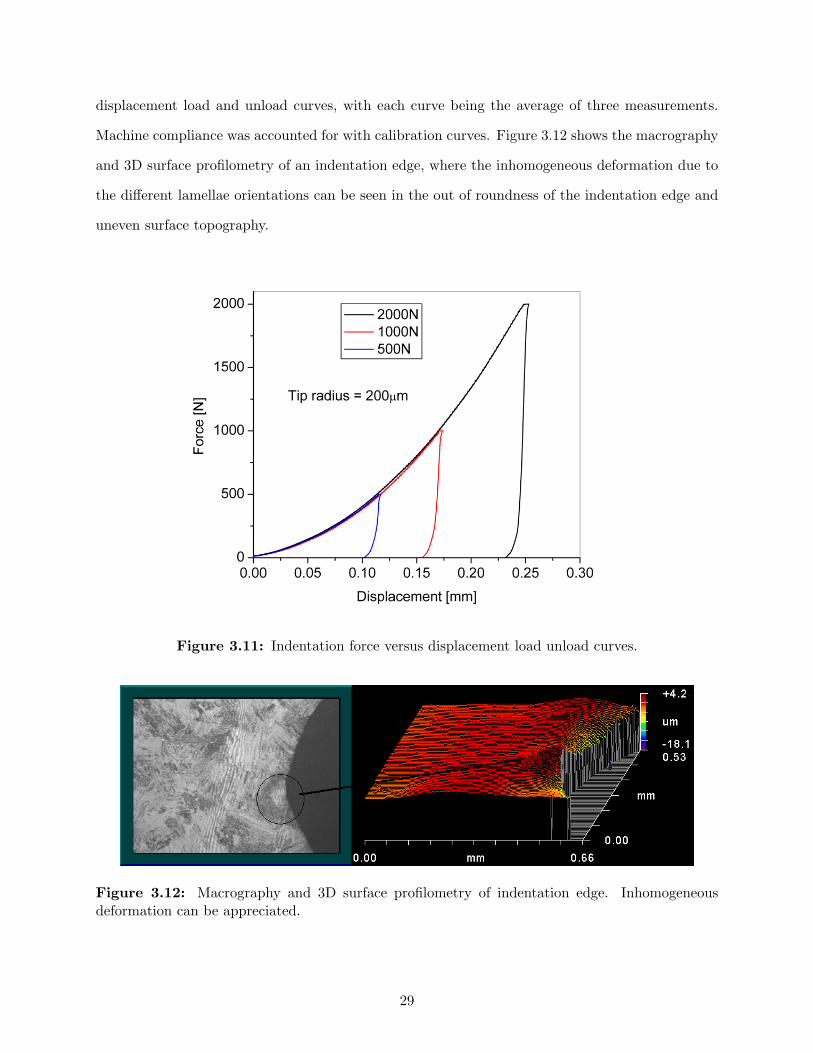
displacement load and unload curves, with each curve being the average of three measurements.
Machine compliance was accounted for with calibration curves. Figure 3.12 shows the macrography
and 3D surface profilometry of an indentation edge, where the inhomogeneous deformation due to
the different lamellae orientations can be seen in the out of roundness of the indentation edge and
uneven surface topography.
Figure 3.11: Indentation force versus displacement load unload curves.
Figure 3.12: Macrography and 3D surface profilometry of indentation edge. Inhomogeneousdeformation can be appreciated.
29
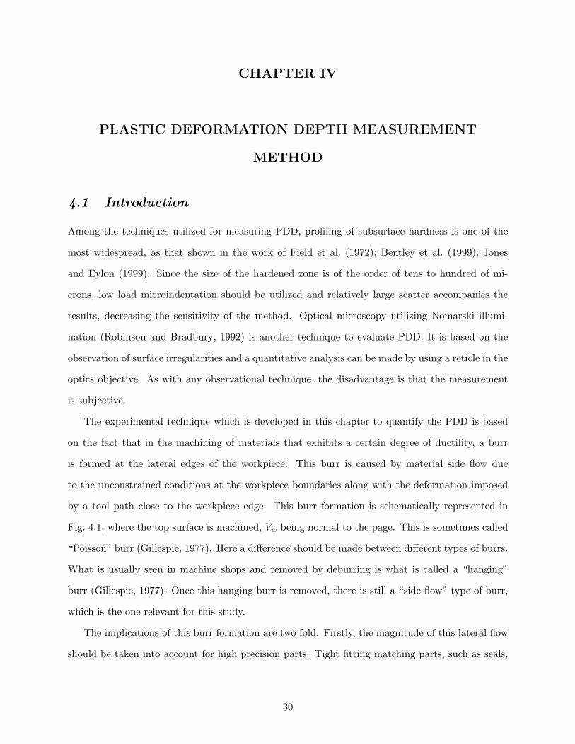
CHAPTER IV
PLASTIC DEFORMATION DEPTH MEASUREMENT
METHOD
4.1 Introduction
Among the techniques utilized for measuring PDD, profiling of subsurface hardness is one of the
most widespread, as that shown in the work of Field et al. (1972); Bentley et al. (1999); Jones
and Eylon (1999). Since the size of the hardened zone is of the order of tens to hundred of mi-
crons, low load microindentation should be utilized and relatively large scatter accompanies the
results, decreasing the sensitivity of the method. Optical microscopy utilizing Nomarski illumi-
nation (Robinson and Bradbury, 1992) is another technique to evaluate PDD. It is based on the
observation of surface irregularities and a quantitative analysis can be made by using a reticle in the
optics objective. As with any observational technique, the disadvantage is that the measurement
is subjective.
The experimental technique which is developed in this chapter to quantify the PDD is based
on the fact that in the machining of materials that exhibits a certain degree of ductility, a burr
is formed at the lateral edges of the workpiece. This burr is caused by material side flow due
to the unconstrained conditions at the workpiece boundaries along with the deformation imposed
by a tool path close to the workpiece edge. This burr formation is schematically represented in
Fig. 4.1, where the top surface is machined, Vw being normal to the page. This is sometimes called
“Poisson” burr (Gillespie, 1977). Here a difference should be made between different types of burrs.
What is usually seen in machine shops and removed by deburring is what is called a “hanging”
burr (Gillespie, 1977). Once this hanging burr is removed, there is still a “side flow” type of burr,
which is the one relevant for this study.
The implications of this burr formation are two fold. Firstly, the magnitude of this lateral flow
should be taken into account for high precision parts. Tight fitting matching parts, such as seals,
30
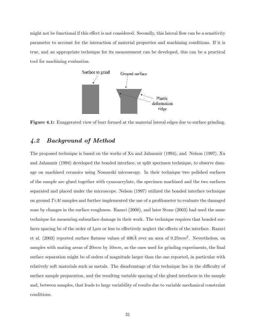
might not be functional if this effect is not considered. Secondly, this lateral flow can be a sensitivity
parameter to account for the interaction of material properties and machining conditions. If it is
true, and an appropriate technique for its measurement can be developed, this can be a practical
tool for machining evaluation.
Figure 4.1: Exaggerated view of burr formed at the material lateral edges due to surface grinding.
4.2 Background of Method
The proposed technique is based on the works of Xu and Jahanmir (1994), and Nelson (1997). Xu
and Jahanmir (1994) developed the bonded interface, or split specimen technique, to observe dam-
age on machined ceramics using Nomarski microscopy. In their technique two polished surfaces
of the sample are glued together with cyanoacrylate, the specimen machined and the two surfaces
separated and placed under the microscope. Nelson (1997) utilized the bonded interface technique
on ground TiAl samples and further implemented the use of a profilometer to evaluate the damaged
zone by changes in the surface roughness. Razavi (2000), and later Stone (2003) had used the same
technique for measuring subsurface damage in their work. The technique requires that bonded sur-
faces spacing be of the order of 1µm or less to effectively neglect the effects of the interface. Razavi
et al. (2003) reported surface flatness values of 400A over an area of 0.25mm2. Nevertheless, on
samples with mating areas of 20mm by 10mm, as the ones used for grinding experiments, the final
surface separation might be of orders of magnitude larger than the one reported, in particular with
relatively soft materials such as metals. The disadvantage of this technique lies in the difficulty of
surface sample preparation, and the resulting variable spacing of the glued interfaces in the sample
and, between samples, that leads to large variability of results due to variable mechanical constraint
conditions.
31
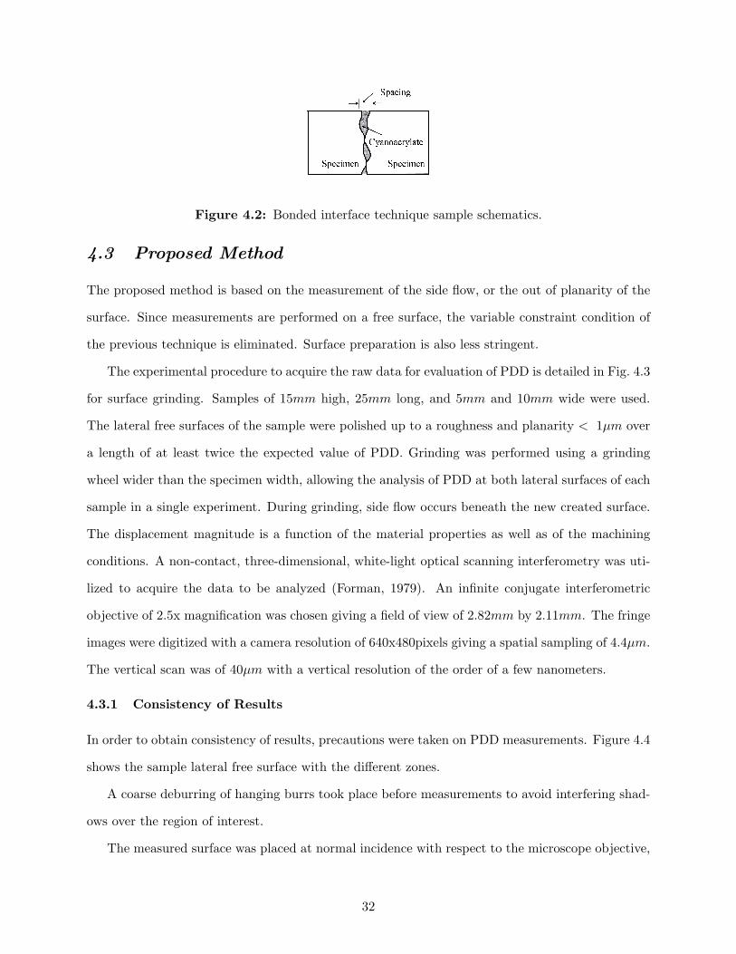
Figure 4.2: Bonded interface technique sample schematics.
4.3 Proposed Method
The proposed method is based on the measurement of the side flow, or the out of planarity of the
surface. Since measurements are performed on a free surface, the variable constraint condition of
the previous technique is eliminated. Surface preparation is also less stringent.
The experimental procedure to acquire the raw data for evaluation of PDD is detailed in Fig. 4.3
for surface grinding. Samples of 15mm high, 25mm long, and 5mm and 10mm wide were used.
The lateral free surfaces of the sample were polished up to a roughness and planarity < 1µm over
a length of at least twice the expected value of PDD. Grinding was performed using a grinding
wheel wider than the specimen width, allowing the analysis of PDD at both lateral surfaces of each
sample in a single experiment. During grinding, side flow occurs beneath the new created surface.
The displacement magnitude is a function of the material properties as well as of the machining
conditions. A non-contact, three-dimensional, white-light optical scanning interferometry was uti-
lized to acquire the data to be analyzed (Forman, 1979). An infinite conjugate interferometric
objective of 2.5x magnification was chosen giving a field of view of 2.82mm by 2.11mm. The fringe
images were digitized with a camera resolution of 640x480pixels giving a spatial sampling of 4.4µm.
The vertical scan was of 40µm with a vertical resolution of the order of a few nanometers.
4.3.1 Consistency of Results
In order to obtain consistency of results, precautions were taken on PDD measurements. Figure 4.4
shows the sample lateral free surface with the different zones.
A coarse deburring of hanging burrs took place before measurements to avoid interfering shad-
ows over the region of interest.
The measured surface was placed at normal incidence with respect to the microscope objective,
32
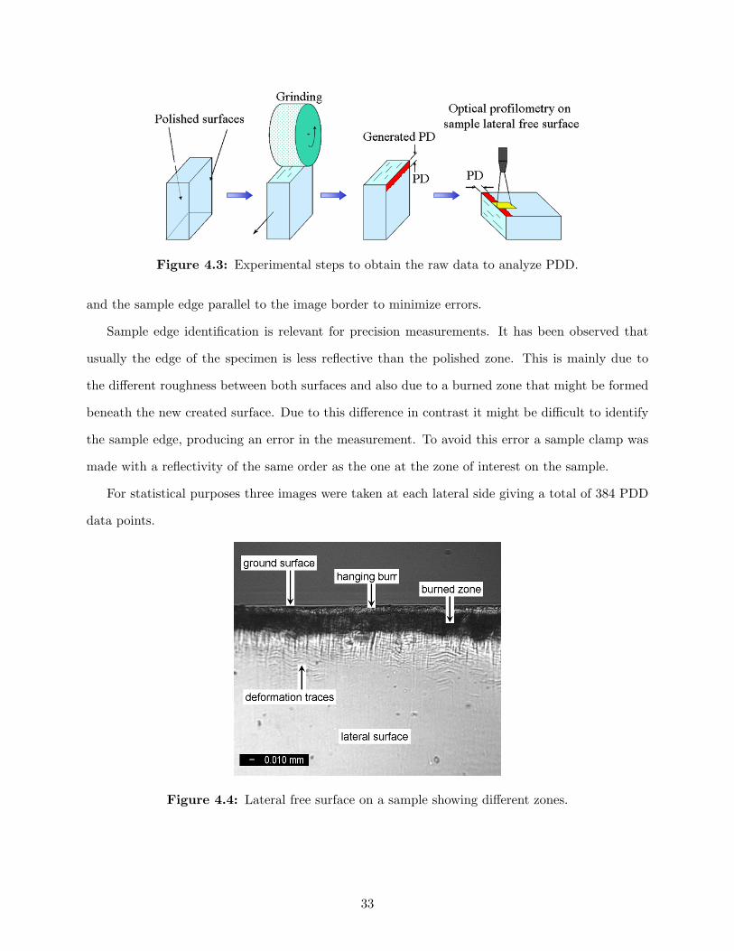
Figure 4.3: Experimental steps to obtain the raw data to analyze PDD.
and the sample edge parallel to the image border to minimize errors.
Sample edge identification is relevant for precision measurements. It has been observed that
usually the edge of the specimen is less reflective than the polished zone. This is mainly due to
the different roughness between both surfaces and also due to a burned zone that might be formed
beneath the new created surface. Due to this difference in contrast it might be difficult to identify
the sample edge, producing an error in the measurement. To avoid this error a sample clamp was
made with a reflectivity of the same order as the one at the zone of interest on the sample.
For statistical purposes three images were taken at each lateral side giving a total of 384 PDD
data points.
Figure 4.4: Lateral free surface on a sample showing different zones.
33
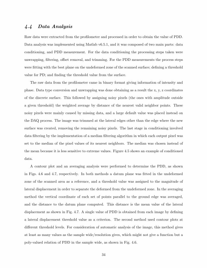
4.4 Data Analysis
Raw data were extracted from the profilometer and processed in order to obtain the value of PDD.
Data analysis was implemented using Matlab v6.5.1, and it was composed of two main parts: data
conditioning, and PDD measurement. For the data conditioning the processing steps taken were
unwrapping, filtering, offset removal, and trimming. For the PDD measurements the process steps
were fitting with the best plane on the undeformed zone of the scanned surface; defining a threshold
value for PD; and finding the threshold value from the surface.
The raw data from the profilometer came in binary format giving information of intensity and
phase. Data type conversion and unwrapping was done obtaining as a result the x, y, z coordinates
of the discrete surface. This followed by assigning noisy pixels (the ones with amplitude outside
a given threshold) the weighted average by distance of the nearest valid neighbor points. These
noisy pixels were mainly caused by missing data, and a large default value was placed instead on
the DAQ process. The image was trimmed at the lateral edges other than the edge where the new
surface was created, removing the remaining noisy pixels. The last stage in conditioning involved
data filtering by the implementation of a median filtering algorithm in which each output pixel was
set to the median of the pixel values of its nearest neighbors. The median was chosen instead of
the mean because it is less sensitive to extreme values. Figure 4.5 shows an example of conditioned
data.
A contour plot and an averaging analysis were performed to determine the PDD, as shown
in Figs. 4.6 and 4.7, respectively. In both methods a datum plane was fitted in the undeformed
zone of the scanned area as a reference, and a threshold value was assigned to the magnitude of
lateral displacement in order to separate the deformed from the undeformed zone. In the averaging
method the vertical coordinate of each set of points parallel to the ground edge was averaged,
and the distance to the datum plane computed. This distance is the mean value of the lateral
displacement as shown in Fig. 4.7. A single value of PDD is obtained from each image by defining
a lateral displacement threshold value as a criterion. The second method used contour plots at
different threshold levels. For consideration of automatic analysis of the image, this method gives
at least as many values as the sample wide/resolution gives, which might not give a function but a
poly-valued relation of PDD in the sample wide, as shown in Fig. 4.6.
34
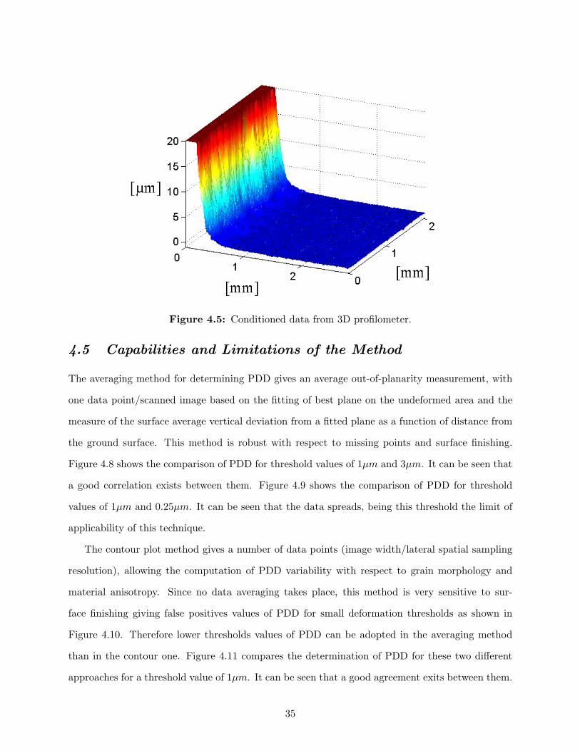
Figure 4.5: Conditioned data from 3D profilometer.
4.5 Capabilities and Limitations of the Method
The averaging method for determining PDD gives an average out-of-planarity measurement, with
one data point/scanned image based on the fitting of best plane on the undeformed area and the
measure of the surface average vertical deviation from a fitted plane as a function of distance from
the ground surface. This method is robust with respect to missing points and surface finishing.
Figure 4.8 shows the comparison of PDD for threshold values of 1µm and 3µm. It can be seen that
a good correlation exists between them. Figure 4.9 shows the comparison of PDD for threshold
values of 1µm and 0.25µm. It can be seen that the data spreads, being this threshold the limit of
applicability of this technique.
The contour plot method gives a number of data points (image width/lateral spatial sampling
resolution), allowing the computation of PDD variability with respect to grain morphology and
material anisotropy. Since no data averaging takes place, this method is very sensitive to sur-
face finishing giving false positives values of PDD for small deformation thresholds as shown in
Figure 4.10. Therefore lower thresholds values of PDD can be adopted in the averaging method
than in the contour one. Figure 4.11 compares the determination of PDD for these two different
approaches for a threshold value of 1µm. It can be seen that a good agreement exits between them.
35
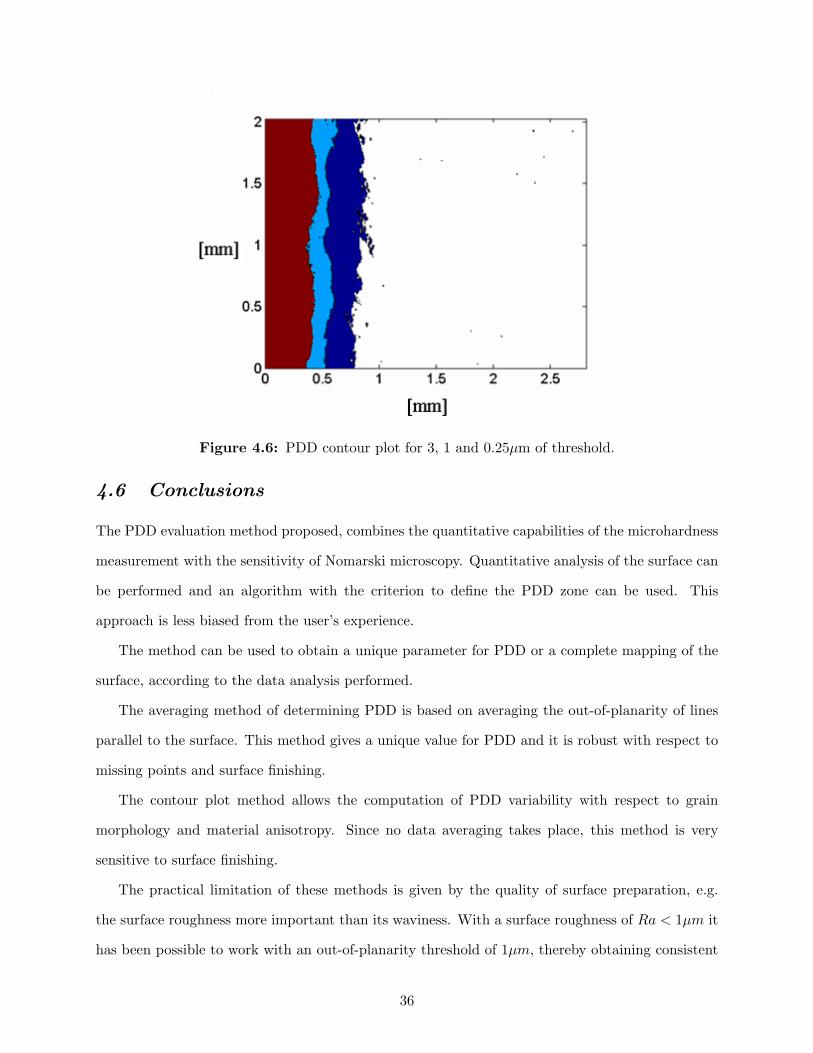
Figure 4.6: PDD contour plot for 3, 1 and 0.25µm of threshold.
4.6 Conclusions
The PDD evaluation method proposed, combines the quantitative capabilities of the microhardness
measurement with the sensitivity of Nomarski microscopy. Quantitative analysis of the surface can
be performed and an algorithm with the criterion to define the PDD zone can be used. This
approach is less biased from the user’s experience.
The method can be used to obtain a unique parameter for PDD or a complete mapping of the
surface, according to the data analysis performed.
The averaging method of determining PDD is based on averaging the out-of-planarity of lines
parallel to the surface. This method gives a unique value for PDD and it is robust with respect to
missing points and surface finishing.
The contour plot method allows the computation of PDD variability with respect to grain
morphology and material anisotropy. Since no data averaging takes place, this method is very
sensitive to surface finishing.
The practical limitation of these methods is given by the quality of surface preparation, e.g.
the surface roughness more important than its waviness. With a surface roughness of Ra < 1µm it
has been possible to work with an out-of-planarity threshold of 1µm, thereby obtaining consistent
36
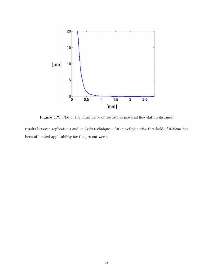
Figure 4.7: Plot of the mean value of the lateral material flow-datum distance.
results between replications and analysis techniques. An out-of-planarity threshold of 0.25µm has
been of limited applicability for the present work.
37
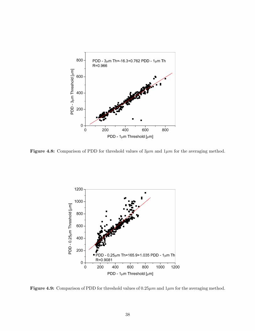
Figure 4.8: Comparison of PDD for threshold values of 3µm and 1µm for the averaging method.
Figure 4.9: Comparison of PDD for threshold values of 0.25µm and 1µm for the averaging method.
38
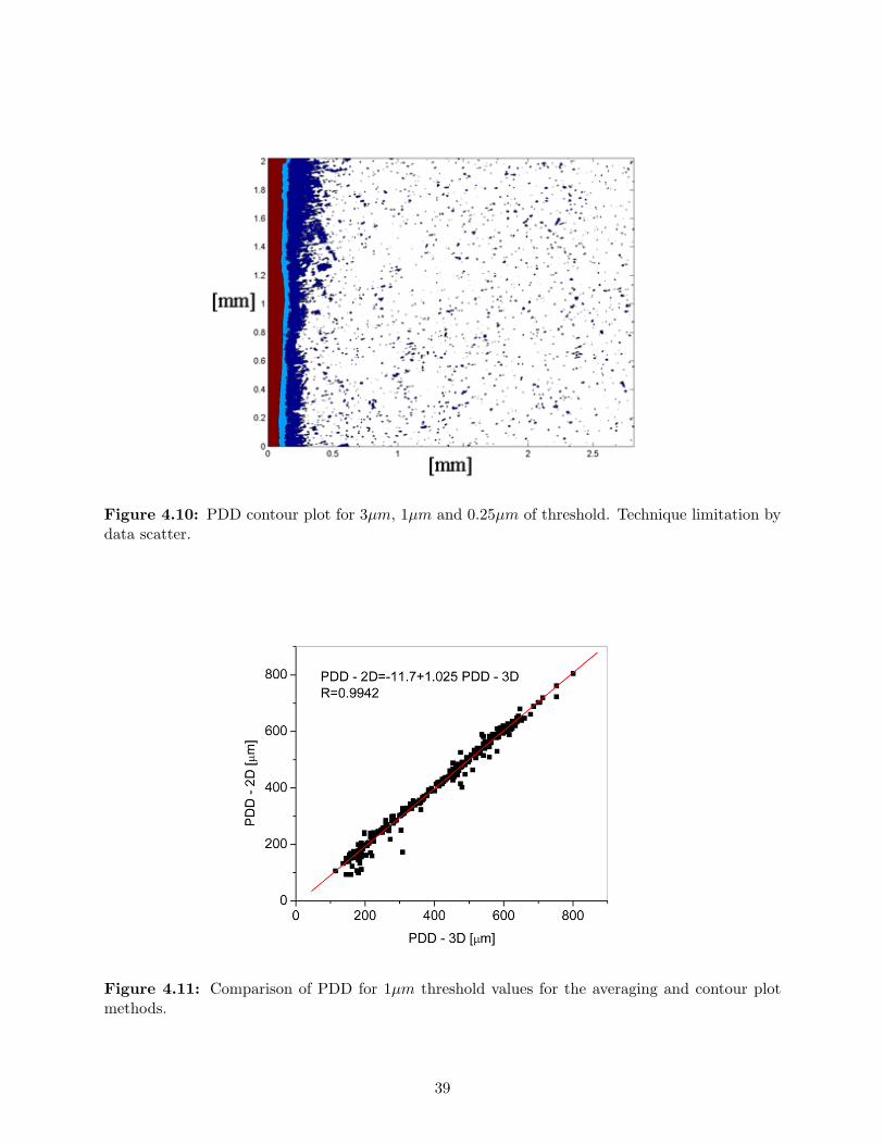
Figure 4.10: PDD contour plot for 3µm, 1µm and 0.25µm of threshold. Technique limitation bydata scatter.
Figure 4.11: Comparison of PDD for 1µm threshold values for the averaging and contour plotmethods.
39
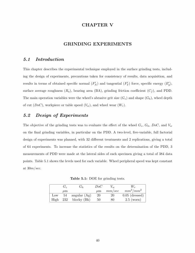
CHAPTER V
GRINDING EXPERIMENTS
5.1 Introduction
This chapter describes the experimental technique employed in the surface grinding tests, includ-
ing the design of experiments, precautions taken for consistency of results, data acquisition, and
results in terms of obtained specific normal (F ′N ) and tangential (F ′
T ) force, specific energy (E′g),
surface average roughness (Ra), bearing area (BA), grinding friction coefficient (Cf ), and PDD.
The main operation variables were the wheel’s abrasive grit size (Gz) and shape (Gh), wheel depth
of cut (DoC), workpiece or table speed (Vw), and wheel wear (Wr).
5.2 Design of Experiments
The objective of the grinding tests was to evaluate the effect of the wheel Gz, Gh, DoC, and Vw
on the final grinding variables, in particular on the PDD. A two-level, five-variable, full factorial
design of experiments was planned, with 32 different treatments and 2 replications, giving a total
of 64 experiments. To increase the statistics of the results on the determination of the PDD, 3
measurements of PDD were made at the lateral sides of each specimen giving a total of 384 data
points. Table 5.1 shows the levels used for each variable. Wheel peripheral speed was kept constant
at 30m/sec.
Table 5.1: DOE for grinding tests.
Gz Gh DoC Vw Wr
µm µm mm/sec mm3/mm2
Low 54 angular (Ag) 20 20 0.05 (dressed)High 232 blocky (Bk) 50 80 2.5 (worn)
40
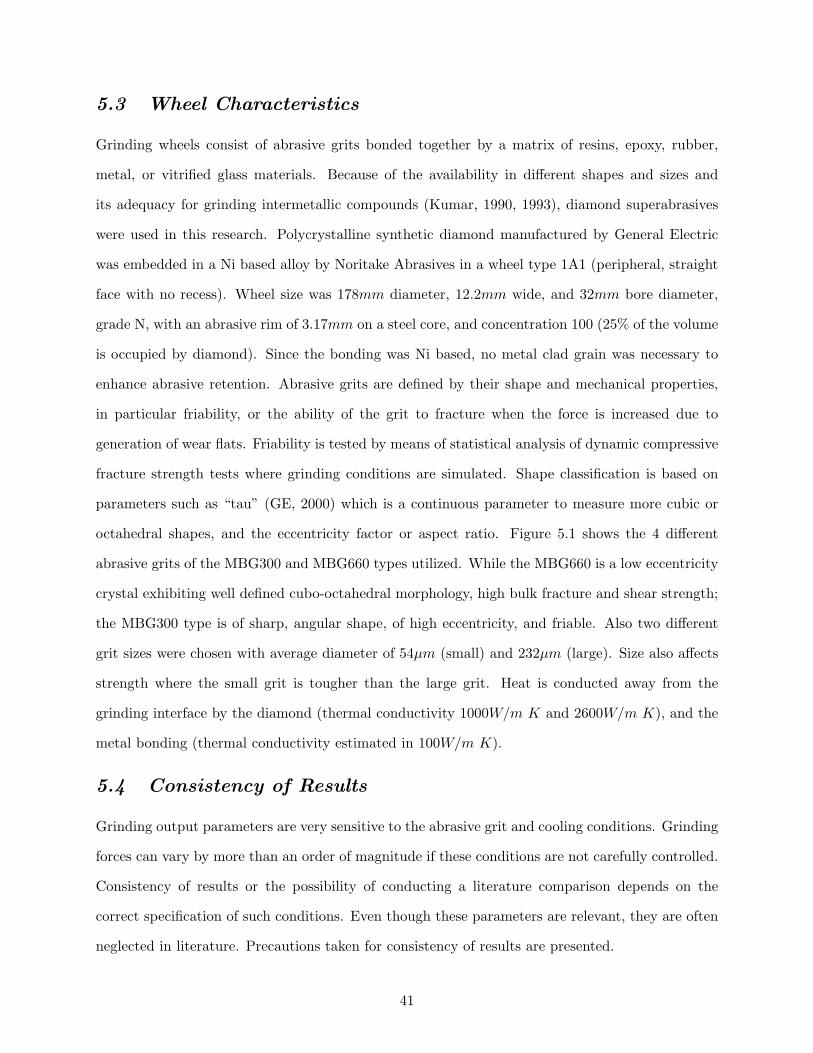
5.3 Wheel Characteristics
Grinding wheels consist of abrasive grits bonded together by a matrix of resins, epoxy, rubber,
metal, or vitrified glass materials. Because of the availability in different shapes and sizes and
its adequacy for grinding intermetallic compounds (Kumar, 1990, 1993), diamond superabrasives
were used in this research. Polycrystalline synthetic diamond manufactured by General Electric
was embedded in a Ni based alloy by Noritake Abrasives in a wheel type 1A1 (peripheral, straight
face with no recess). Wheel size was 178mm diameter, 12.2mm wide, and 32mm bore diameter,
grade N, with an abrasive rim of 3.17mm on a steel core, and concentration 100 (25% of the volume
is occupied by diamond). Since the bonding was Ni based, no metal clad grain was necessary to
enhance abrasive retention. Abrasive grits are defined by their shape and mechanical properties,
in particular friability, or the ability of the grit to fracture when the force is increased due to
generation of wear flats. Friability is tested by means of statistical analysis of dynamic compressive
fracture strength tests where grinding conditions are simulated. Shape classification is based on
parameters such as “tau” (GE, 2000) which is a continuous parameter to measure more cubic or
octahedral shapes, and the eccentricity factor or aspect ratio. Figure 5.1 shows the 4 different
abrasive grits of the MBG300 and MBG660 types utilized. While the MBG660 is a low eccentricity
crystal exhibiting well defined cubo-octahedral morphology, high bulk fracture and shear strength;
the MBG300 type is of sharp, angular shape, of high eccentricity, and friable. Also two different
grit sizes were chosen with average diameter of 54µm (small) and 232µm (large). Size also affects
strength where the small grit is tougher than the large grit. Heat is conducted away from the
grinding interface by the diamond (thermal conductivity 1000W/m K and 2600W/m K), and the
metal bonding (thermal conductivity estimated in 100W/m K).
5.4 Consistency of Results
Grinding output parameters are very sensitive to the abrasive grit and cooling conditions. Grinding
forces can vary by more than an order of magnitude if these conditions are not carefully controlled.
Consistency of results or the possibility of conducting a literature comparison depends on the
correct specification of such conditions. Even though these parameters are relevant, they are often
neglected in literature. Precautions taken for consistency of results are presented.
41
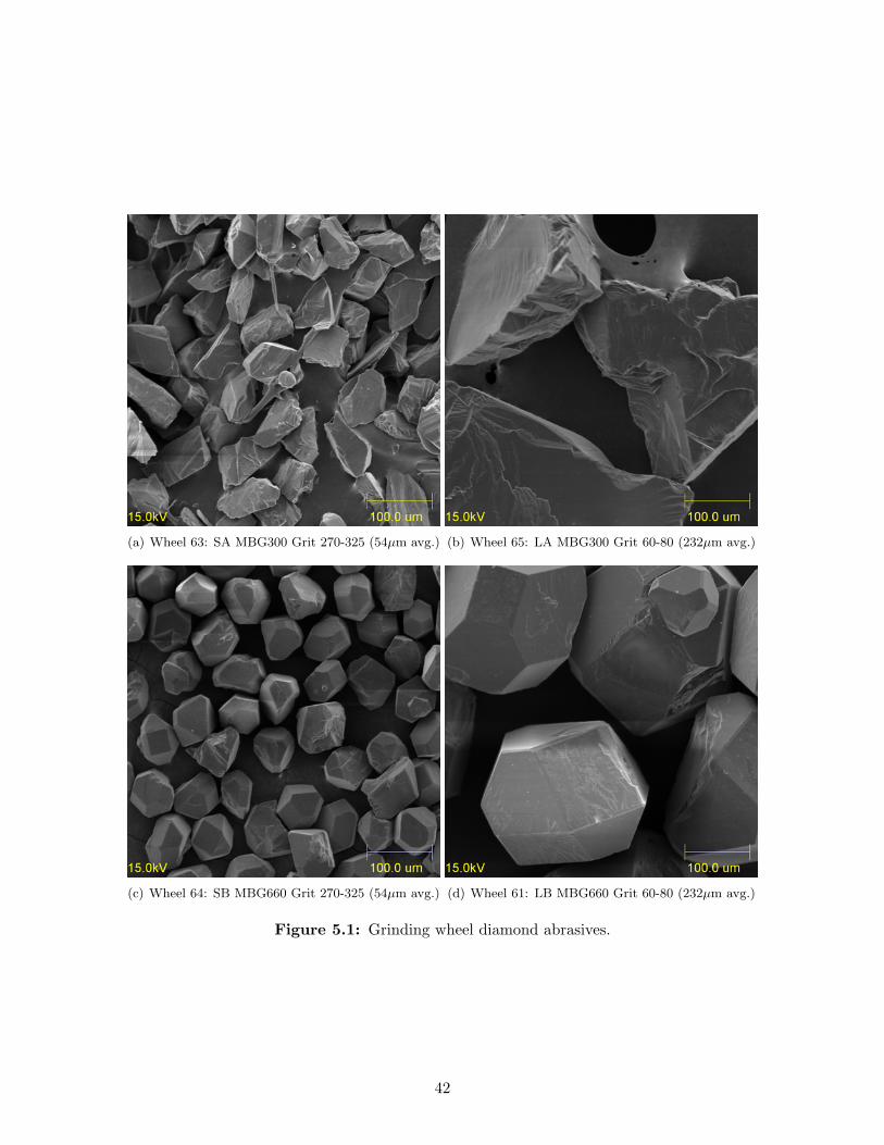
(a) Wheel 63: SA MBG300 Grit 270-325 (54µm avg.) (b) Wheel 65: LA MBG300 Grit 60-80 (232µm avg.)
(c) Wheel 64: SB MBG660 Grit 270-325 (54µm avg.) (d) Wheel 61: LB MBG660 Grit 60-80 (232µm avg.)
Figure 5.1: Grinding wheel diamond abrasives.
42
5.4.1 Wheel Wear
After the wheel is conditioned by truing and dressing, abrasives have sharp cutting edges that
gradually become dull with use, mainly by generation of wear flats. The more friable the abrasive,
the easier it can fracture allowing new edges to be generated. The process of wear flat generation
and grit fracture might not reach an equilibrium, therefore grinding is generally done under variable
conditions. Figure 5.2 shows the effects of the abrasive wear on the normal force. Each point on
the plot represents a grinding reciprocating cycle. The first 5 to 10 points usually showed a step
increase in the normal force due to the machine compliance and the displacement control given by
the DoC. Machine compliance becomes irrelevant if DoC control is used and kept constant during
the tests, while enough cycles are set and the steady state reached. The upper abscissa shows the
specific material removal per unit width. The lower one shows the wheel specific material removal
which adds the normalization by the wheel perimeter. This latter measure is not commonly used
in the literature because a unique wheel diameter is assumed. The normal force is represented by
its plateau value at each cycle, as shown in Figure 5.3. One way to control the wear effects is by
implementing continuous dressing (Ohmori et al., 1996). To obtain consistent results, the same
amount of material was removed in each test.
Figure 5.2: Effects of abrasive wear on the normal force.
43
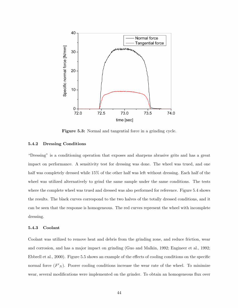
Figure 5.3: Normal and tangential force in a grinding cycle.
5.4.2 Dressing Conditions
“Dressing” is a conditioning operation that exposes and sharpens abrasive grits and has a great
impact on performance. A sensitivity test for dressing was done. The wheel was trued, and one
half was completely dressed while 15% of the other half was left without dressing. Each half of the
wheel was utilized alternatively to grind the same sample under the same conditions. The tests
where the complete wheel was trued and dressed was also performed for reference. Figure 5.4 shows
the results. The black curves correspond to the two halves of the totally dressed conditions, and it
can be seen that the response is homogeneous. The red curves represent the wheel with incomplete
dressing.
5.4.3 Coolant
Coolant was utilized to remove heat and debris from the grinding zone, and reduce friction, wear
and corrosion, and has a major impact on grinding (Guo and Malkin, 1992; Engineer et al., 1992;
Ebbrell et al., 2000). Figure 5.5 shows an example of the effects of cooling conditions on the specific
normal force (F ′N ). Poorer cooling conditions increase the wear rate of the wheel. To minimize
wear, several modifications were implemented on the grinder. To obtain an homogeneous flux over
44
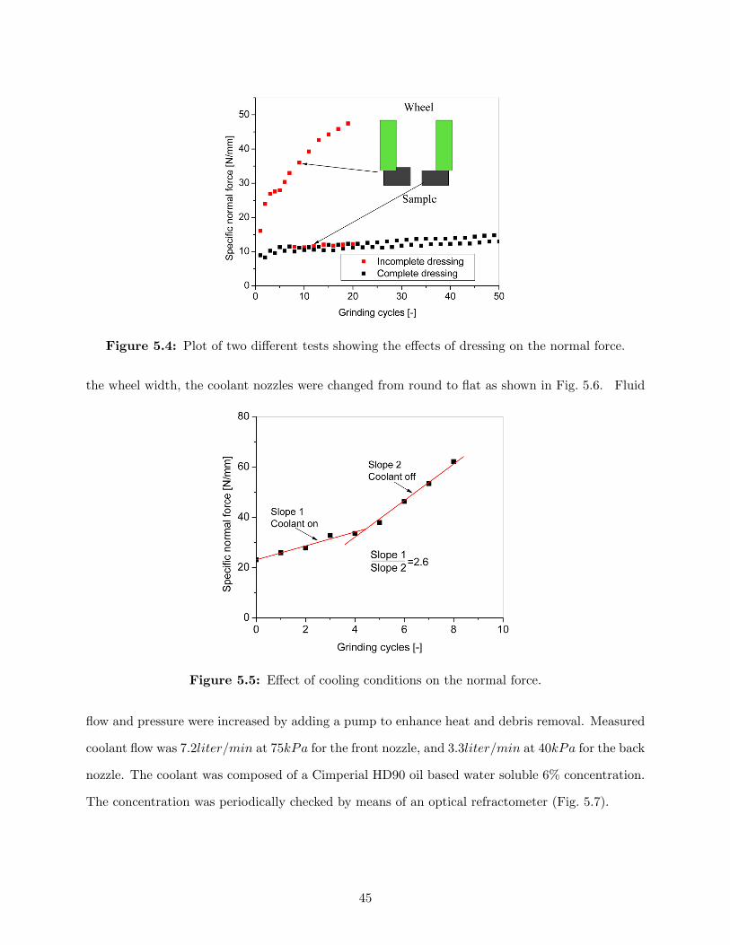
Figure 5.4: Plot of two different tests showing the effects of dressing on the normal force.
the wheel width, the coolant nozzles were changed from round to flat as shown in Fig. 5.6. Fluid
Figure 5.5: Effect of cooling conditions on the normal force.
flow and pressure were increased by adding a pump to enhance heat and debris removal. Measured
coolant flow was 7.2liter/min at 75kPa for the front nozzle, and 3.3liter/min at 40kPa for the back
nozzle. The coolant was composed of a Cimperial HD90 oil based water soluble 6% concentration.
The concentration was periodically checked by means of an optical refractometer (Fig. 5.7).
45
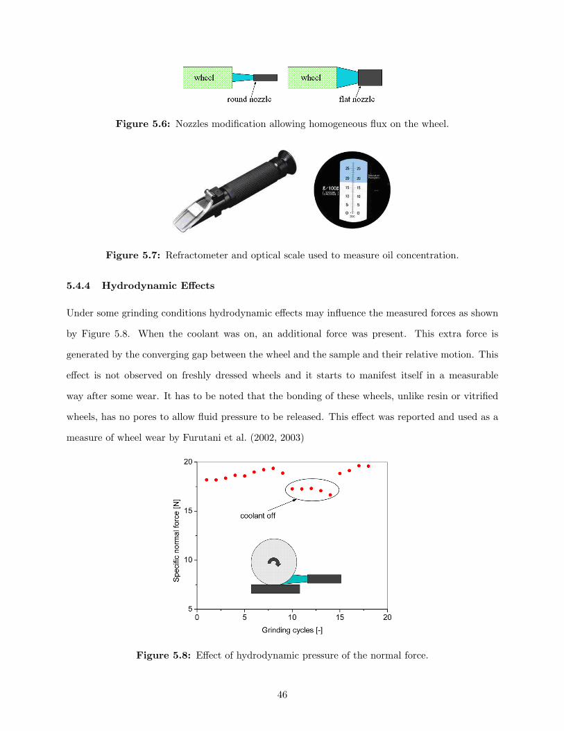
Figure 5.6: Nozzles modification allowing homogeneous flux on the wheel.
Figure 5.7: Refractometer and optical scale used to measure oil concentration.
5.4.4 Hydrodynamic Effects
Under some grinding conditions hydrodynamic effects may influence the measured forces as shown
by Figure 5.8. When the coolant was on, an additional force was present. This extra force is
generated by the converging gap between the wheel and the sample and their relative motion. This
effect is not observed on freshly dressed wheels and it starts to manifest itself in a measurable
way after some wear. It has to be noted that the bonding of these wheels, unlike resin or vitrified
wheels, has no pores to allow fluid pressure to be released. This effect was reported and used as a
measure of wheel wear by Furutani et al. (2002, 2003)
Figure 5.8: Effect of hydrodynamic pressure of the normal force.
46
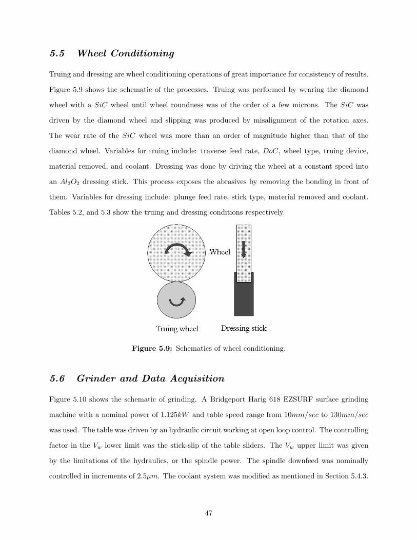
5.5 Wheel Conditioning
Truing and dressing are wheel conditioning operations of great importance for consistency of results.
Figure 5.9 shows the schematic of the processes. Truing was performed by wearing the diamond
wheel with a SiC wheel until wheel roundness was of the order of a few microns. The SiC was
driven by the diamond wheel and slipping was produced by misalignment of the rotation axes.
The wear rate of the SiC wheel was more than an order of magnitude higher than that of the
diamond wheel. Variables for truing include: traverse feed rate, DoC, wheel type, truing device,
material removed, and coolant. Dressing was done by driving the wheel at a constant speed into
an Al3O2 dressing stick. This process exposes the abrasives by removing the bonding in front of
them. Variables for dressing include: plunge feed rate, stick type, material removed and coolant.
Tables 5.2, and 5.3 show the truing and dressing conditions respectively.
Figure 5.9: Schematics of wheel conditioning.
5.6 Grinder and Data Acquisition
Figure 5.10 shows the schematic of grinding. A Bridgeport Harig 618 EZSURF surface grinding
machine with a nominal power of 1.125kW and table speed range from 10mm/sec to 130mm/sec
was used. The table was driven by an hydraulic circuit working at open loop control. The controlling
factor in the Vw lower limit was the stick-slip of the table sliders. The Vw upper limit was given
by the limitations of the hydraulics, or the spindle power. The spindle downfeed was nominally
controlled in increments of 2.5µm. The coolant system was modified as mentioned in Section 5.4.3.
47
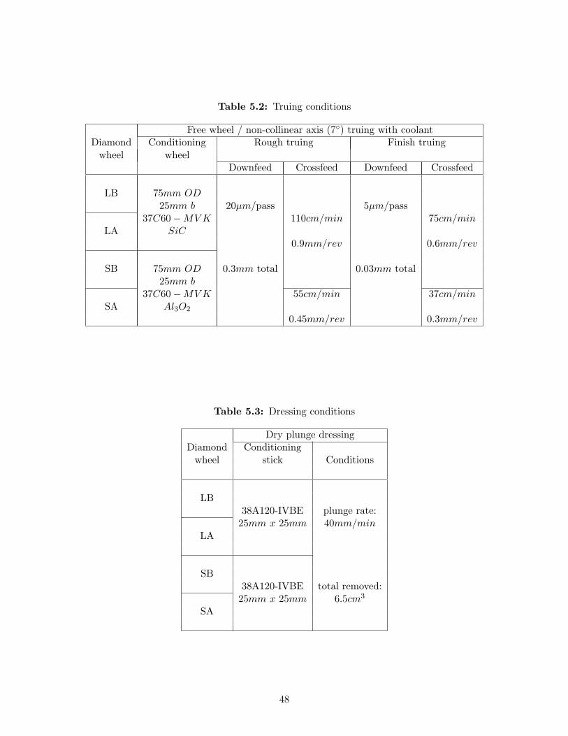
Table 5.2: Truing conditions
Free wheel / non-collinear axis (7) truing with coolantDiamond Conditioning Rough truing Finish truing
wheel wheelDownfeed Crossfeed Downfeed Crossfeed
LB 75mm OD25mm b 20µm/pass 5µm/pass
37C60−MV K 110cm/min 75cm/minLA SiC
0.9mm/rev 0.6mm/rev
SB 75mm OD 0.3mm total 0.03mm total25mm b
37C60−MV K 55cm/min 37cm/minSA Al3O2
0.45mm/rev 0.3mm/rev
Table 5.3: Dressing conditions
Dry plunge dressingDiamond Conditioning
wheel stick Conditions
LB38A120-IVBE plunge rate:
25mm x 25mm 40mm/minLA
SB38A120-IVBE total removed:
25mm x 25mm 6.5cm3
SA
48
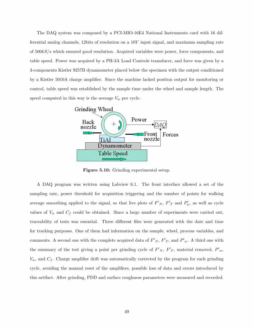
The DAQ system was composed by a PCI-MIO-16E4 National Instruments card with 16 dif-
ferential analog channels, 12bits of resolution on a 10V input signal, and maximum sampling rate
of 500kS/s which ensured good resolution. Acquired variables were power, force components, and
table speed. Power was acquired by a PH-3A Load Controls transducer, and force was given by a
3-components Kistler 9257B dynamometer placed below the specimen with the output conditioned
by a Kistler 5010A charge amplifier. Since the machine lacked position output for monitoring or
control, table speed was established by the sample time under the wheel and sample length. The
speed computed in this way is the average Vw per cycle.
Figure 5.10: Grinding experimental setup.
A DAQ program was written using Labview 6.1. The front interface allowed a set of the
sampling rate, power threshold for acquisition triggering and the number of points for walking
average smoothing applied to the signal, so that live plots of F ′N , F ′
T and P ′w, as well as cycle
values of Vw and Cf could be obtained. Since a large number of experiments were carried out,
traceability of tests was essential. Three different files were generated with the date and time
for tracking purposes. One of them had information on the sample, wheel, process variables, and
comments. A second one with the complete acquired data of F ′N , F ′
T , and P ′w. A third one with
the summary of the test giving a point per grinding cycle of F ′N , F ′
T , material removed, P ′w,
Vw, and Cf . Charge amplifier drift was automatically corrected by the program for each grinding
cycle, avoiding the manual reset of the amplifiers, possible loss of data and errors introduced by
this artifact. After grinding, PDD and surface roughness parameters were measured and recorded.
49
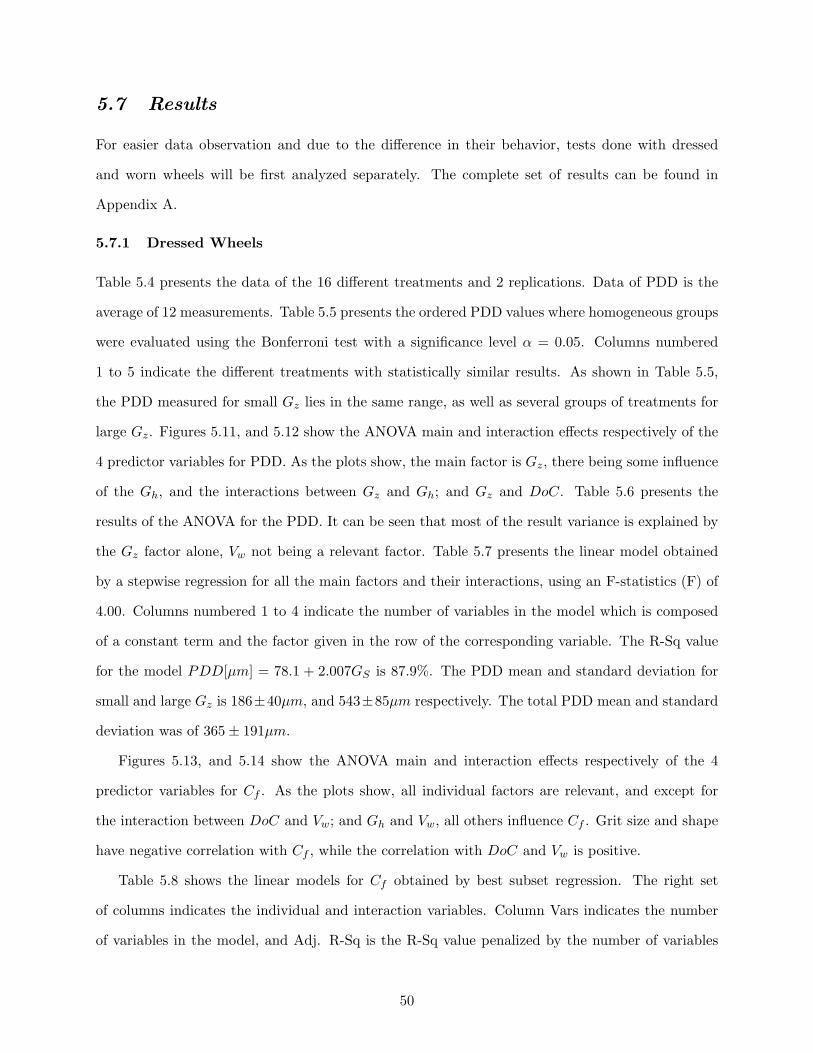
5.7 Results
For easier data observation and due to the difference in their behavior, tests done with dressed
and worn wheels will be first analyzed separately. The complete set of results can be found in
Appendix A.
5.7.1 Dressed Wheels
Table 5.4 presents the data of the 16 different treatments and 2 replications. Data of PDD is the
average of 12 measurements. Table 5.5 presents the ordered PDD values where homogeneous groups
were evaluated using the Bonferroni test with a significance level α = 0.05. Columns numbered
1 to 5 indicate the different treatments with statistically similar results. As shown in Table 5.5,
the PDD measured for small Gz lies in the same range, as well as several groups of treatments for
large Gz. Figures 5.11, and 5.12 show the ANOVA main and interaction effects respectively of the
4 predictor variables for PDD. As the plots show, the main factor is Gz, there being some influence
of the Gh, and the interactions between Gz and Gh; and Gz and DoC. Table 5.6 presents the
results of the ANOVA for the PDD. It can be seen that most of the result variance is explained by
the Gz factor alone, Vw not being a relevant factor. Table 5.7 presents the linear model obtained
by a stepwise regression for all the main factors and their interactions, using an F-statistics (F) of
4.00. Columns numbered 1 to 4 indicate the number of variables in the model which is composed
of a constant term and the factor given in the row of the corresponding variable. The R-Sq value
for the model PDD[µm] = 78.1 + 2.007GS is 87.9%. The PDD mean and standard deviation for
small and large Gz is 186±40µm, and 543±85µm respectively. The total PDD mean and standard
deviation was of 365± 191µm.
Figures 5.13, and 5.14 show the ANOVA main and interaction effects respectively of the 4
predictor variables for Cf . As the plots show, all individual factors are relevant, and except for
the interaction between DoC and Vw; and Gh and Vw, all others influence Cf . Grit size and shape
have negative correlation with Cf , while the correlation with DoC and Vw is positive.
Table 5.8 shows the linear models for Cf obtained by best subset regression. The right set
of columns indicates the individual and interaction variables. Column Vars indicates the number
of variables in the model, and Adj. R-Sq is the R-Sq value penalized by the number of variables
50
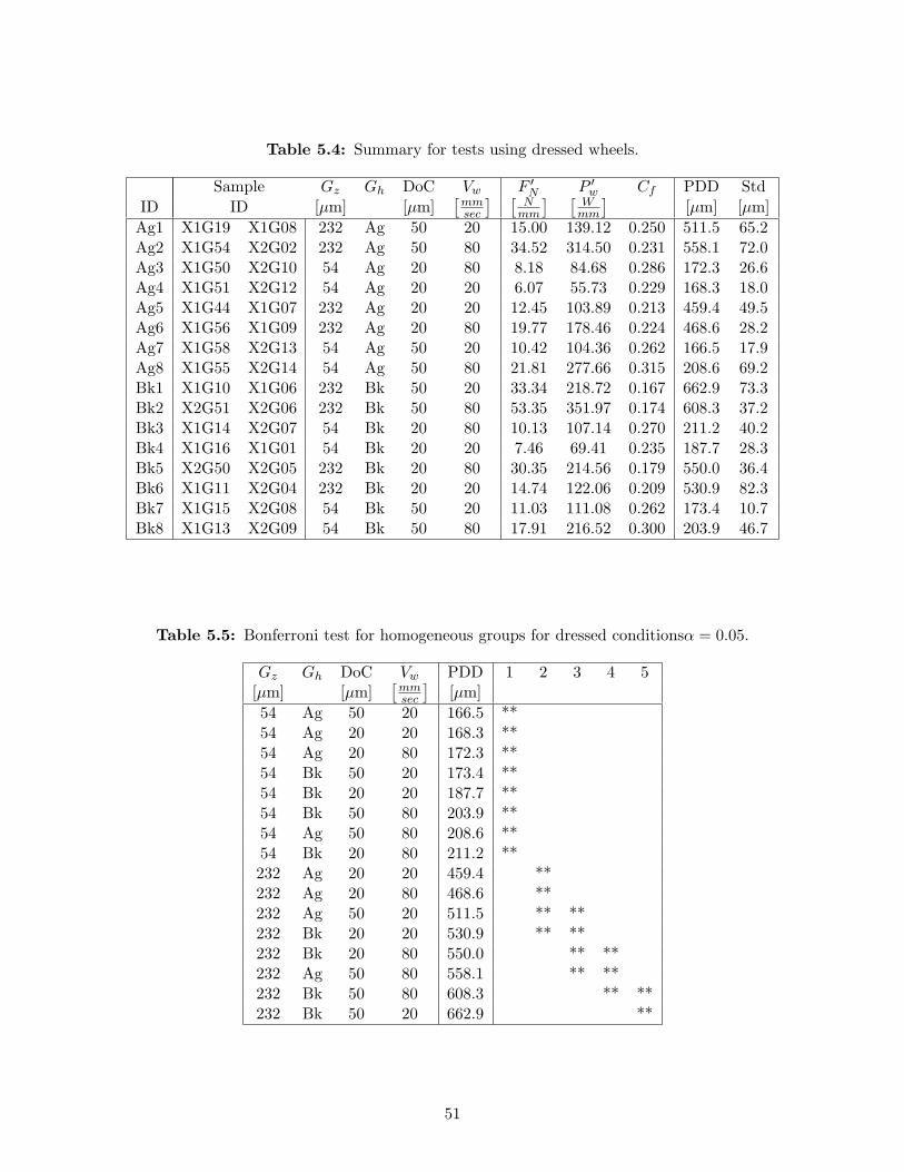
Table 5.4: Summary for tests using dressed wheels.
Sample Gz Gh DoC Vw F ′N P ′
w Cf PDD StdID ID [µm] [µm]
[mmsec
] [N
mm
] [W
mm
][µm] [µm]
Ag1 X1G19 X1G08 232 Ag 50 20 15.00 139.12 0.250 511.5 65.2Ag2 X1G54 X2G02 232 Ag 50 80 34.52 314.50 0.231 558.1 72.0Ag3 X1G50 X2G10 54 Ag 20 80 8.18 84.68 0.286 172.3 26.6Ag4 X1G51 X2G12 54 Ag 20 20 6.07 55.73 0.229 168.3 18.0Ag5 X1G44 X1G07 232 Ag 20 20 12.45 103.89 0.213 459.4 49.5Ag6 X1G56 X1G09 232 Ag 20 80 19.77 178.46 0.224 468.6 28.2Ag7 X1G58 X2G13 54 Ag 50 20 10.42 104.36 0.262 166.5 17.9Ag8 X1G55 X2G14 54 Ag 50 80 21.81 277.66 0.315 208.6 69.2Bk1 X1G10 X1G06 232 Bk 50 20 33.34 218.72 0.167 662.9 73.3Bk2 X2G51 X2G06 232 Bk 50 80 53.35 351.97 0.174 608.3 37.2Bk3 X1G14 X2G07 54 Bk 20 80 10.13 107.14 0.270 211.2 40.2Bk4 X1G16 X1G01 54 Bk 20 20 7.46 69.41 0.235 187.7 28.3Bk5 X2G50 X2G05 232 Bk 20 80 30.35 214.56 0.179 550.0 36.4Bk6 X1G11 X2G04 232 Bk 20 20 14.74 122.06 0.209 530.9 82.3Bk7 X1G15 X2G08 54 Bk 50 20 11.03 111.08 0.262 173.4 10.7Bk8 X1G13 X2G09 54 Bk 50 80 17.91 216.52 0.300 203.9 46.7
Table 5.5: Bonferroni test for homogeneous groups for dressed conditionsα = 0.05.
Gz Gh DoC Vw PDD 1 2 3 4 5[µm] [µm]
[mmsec
][µm]
54 Ag 50 20 166.5 **54 Ag 20 20 168.3 **54 Ag 20 80 172.3 **54 Bk 50 20 173.4 **54 Bk 20 20 187.7 **54 Bk 50 80 203.9 **54 Ag 50 80 208.6 **54 Bk 20 80 211.2 **232 Ag 20 20 459.4 **232 Ag 20 80 468.6 **232 Ag 50 20 511.5 ** **232 Bk 20 20 530.9 ** **232 Bk 20 80 550.0 ** **232 Ag 50 80 558.1 ** **232 Bk 50 80 608.3 ** **232 Bk 50 20 662.9 **
51
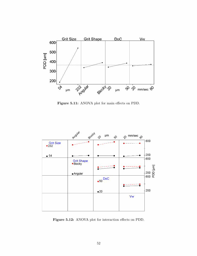
Figure 5.11: ANOVA plot for main effects on PDD.
Figure 5.12: ANOVA plot for interaction effects on PDD.
52
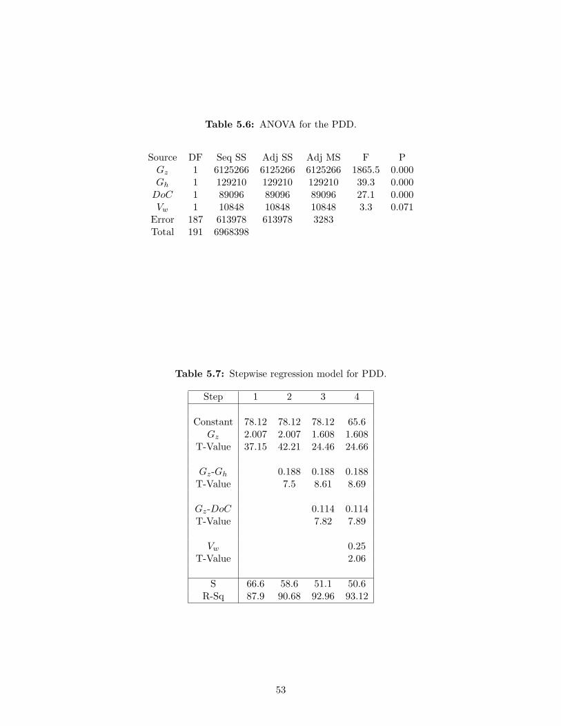
Table 5.6: ANOVA for the PDD.
Source DF Seq SS Adj SS Adj MS F PGz 1 6125266 6125266 6125266 1865.5 0.000Gh 1 129210 129210 129210 39.3 0.000
DoC 1 89096 89096 89096 27.1 0.000Vw 1 10848 10848 10848 3.3 0.071
Error 187 613978 613978 3283Total 191 6968398
Table 5.7: Stepwise regression model for PDD.
Step 1 2 3 4
Constant 78.12 78.12 78.12 65.6Gz 2.007 2.007 1.608 1.608
T-Value 37.15 42.21 24.46 24.66
Gz-Gh 0.188 0.188 0.188T-Value 7.5 8.61 8.69
Gz-DoC 0.114 0.114T-Value 7.82 7.89
Vw 0.25T-Value 2.06
S 66.6 58.6 51.1 50.6R-Sq 87.9 90.68 92.96 93.12
53
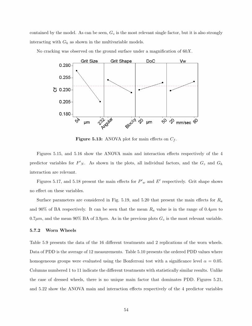
contained by the model. As can be seen, Gz is the most relevant single factor, but it is also strongly
interacting with Gh as shown in the multivariable models.
No cracking was observed on the ground surface under a magnification of 60X.
Figure 5.13: ANOVA plot for main effects on Cf .
Figures 5.15, and 5.16 show the ANOVA main and interaction effects respectively of the 4
predictor variables for F ′N . As shown in the plots, all individual factors, and the Gz and Gh
interaction are relevant.
Figures 5.17, and 5.18 present the main effects for P ′w and E′ respectively. Grit shape shows
no effect on these variables.
Surface parameters are considered in Fig. 5.19, and 5.20 that present the main effects for Ra
and 90% of BA respectively. It can be seen that the mean Ra value is in the range of 0.4µm to
0.7µm, and the mean 90% BA of 3.9µm. As in the previous plots Gz is the most relevant variable.
5.7.2 Worn Wheels
Table 5.9 presents the data of the 16 different treatments and 2 replications of the worn wheels.
Data of PDD is the average of 12 measurements. Table 5.10 presents the ordered PDD values where
homogeneous groups were evaluated using the Bonferroni test with a significance level α = 0.05.
Columns numbered 1 to 11 indicate the different treatments with statistically similar results. Unlike
the case of dressed wheels, there is no unique main factor that dominates PDD. Figures 5.21,
and 5.22 show the ANOVA main and interaction effects respectively of the 4 predictor variables
54
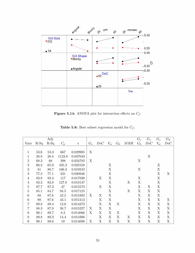
Figure 5.14: ANOVA plot for interaction effects on Cf .
Table 5.8: Best subset regression model for Cf .
Adj. Gz Gz Gz Gh
Vars R-Sq R-Sq Cp s Gz DoC Vw Gh MRR Gh DoC Vw DoC
1 53.6 53.3 667 0.029905 X1 28.8 28.4 1123.8 0.037043 X2 68.3 68 398 0.024782 X X2 66.3 65.9 435.2 0.025558 X X3 81 80.7 166.3 0.019242 X X X3 77.5 77.1 231 0.020946 X X X4 83.8 83.4 117 0.017826 X X X X4 83.2 82.8 127.8 0.018147 X X X X5 87.7 87.3 47 0.015573 X X X X X5 85.1 84.7 94.5 0.017125 X X X X X6 88 87.6 42.5 0.015392 X X X X X X6 88 87.6 43.1 0.015412 X X X X X X7 89.8 89.4 12.6 0.014273 X X X X X X X7 88.3 87.9 38.7 0.015227 X X X X X X X8 90.1 89.7 8.2 0.014066 X X X X X X X X8 89.8 89.3 14.4 0.014306 X X X X X X X X9 90.1 89.6 10 0.014098 X X X X X X X X X
55
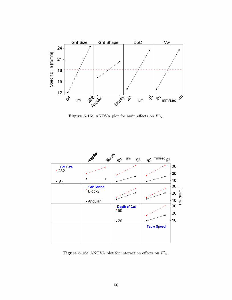
Figure 5.15: ANOVA plot for main effects on F ′N .
Figure 5.16: ANOVA plot for interaction effects on F ′N .
56
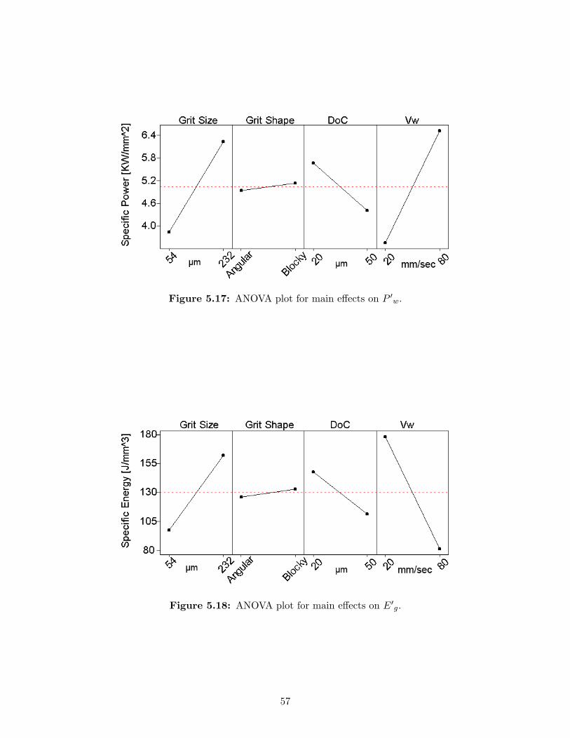
Figure 5.17: ANOVA plot for main effects on P ′w.
Figure 5.18: ANOVA plot for main effects on E′g.
57
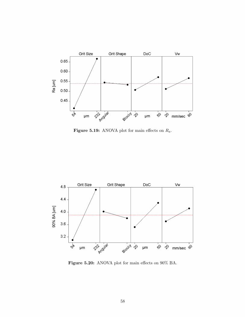
Figure 5.19: ANOVA plot for main effects on Ra.
Figure 5.20: ANOVA plot for main effects on 90% BA.
58
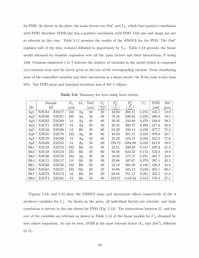
for PDD. As shown in the plots, the main factors are DoC and Vw, which have positive correlation
with PDD, therefore MRR also has a positive correlation with PDD. Grit size and shape are not
so relevant in this case. Table 5.11 presents the results of the ANOVA for the PDD. The DoC
explains half of the data variance followed in importance by Vw. Table 5.12 presents the linear
model obtained by stepwise regression over all the main factors and their interactions, F being
4.00. Columns numbered 1 to 7 indicate the number of variables in the model which is composed
of a constant term and the factor given in the row of the corresponding variable. Even considering
most of the controlled variables and their interaction in a linear model, the R-Sq value is less than
82%. The PDD mean and standard deviation was of 407± 120µm.
Table 5.9: Summary for tests using worn wheels.
Sample Gz Gh DoC Vw F ′N P ′
w Cf PDD StdID ID [µm] [µm]
[mmsec
] [N
mm
] [W
mm
][µm] [µm]
Ag1 X2G84 X2G77 232 Ag 50 20 33.93 288.15 0.213 445.1 18.0Ag2 X2G80 X2G81 232 Ag 50 80 73.48 636.64 0.223 466.8 16.4Ag3 X2G62 X2G68 54 Ag 20 80 38.32 434.80 0.279 238.0 39.2Ag4 X2G71 X2G67 54 Ag 20 20 30.25 360.75 0.293 217.8 33.0Ag5 X2G16 X2G66 54 Bk 20 80 62.29 559.14 0.229 377.7 75.3Ag6 X2G85 X2G76 232 Ag 20 80 40.33 381.75 0.233 378.0 25.7Ag7 X2G70 X2G69 54 Ag 50 20 45.23 524.54 0.280 352.4 17.6Ag8 X2G63 X2G64 54 Ag 50 80 189.72 1082.88 0.160 613.8 59.9Bk1 X2G59 X2G55 232 Bk 50 20 42.51 290.49 0.181 497.9 21.2Bk2 X2G58 X2G54 232 Bk 50 80 92.56 624.23 0.174 553.3 19.8Bk3 X2G86 X2G78 232 Ag 20 20 18.02 175.77 0.251 337.7 23.6Bk4 X2G15 X2G17 54 Bk 20 20 35.06 407.07 0.279 287.1 32.2Bk5 X2G60 X2G56 232 Bk 20 80 52.18 394.26 0.186 428.3 24.6Bk6 X2G61 X2G57 232 Bk 20 20 16.88 165.14 0.249 305.1 68.4Bk7 X2G73 X2G72 54 Bk 50 20 68.04 751.17 0.261 452.5 31.0Bk8 X2G74 X2G65 54 Bk 50 80 162.07 1110.44 0.183 576.4 27.1
Figures 5.23, and 5.24 show the ANOVA main and interaction effects respectively of the 4
predictor variables for Cf . As shown in the plots, all individual factors are relevant, and their
correlation is inverse to the one shown for PDD (Fig. 5.13). The interactions between Gz and the
rest of the variables are relevant as shown in Table 5.13 of the linear models for Cf obtained by
best subset regression. As can be seen, MRR is the most relevant factor (Vw and DoC), followed
by Gz.
59
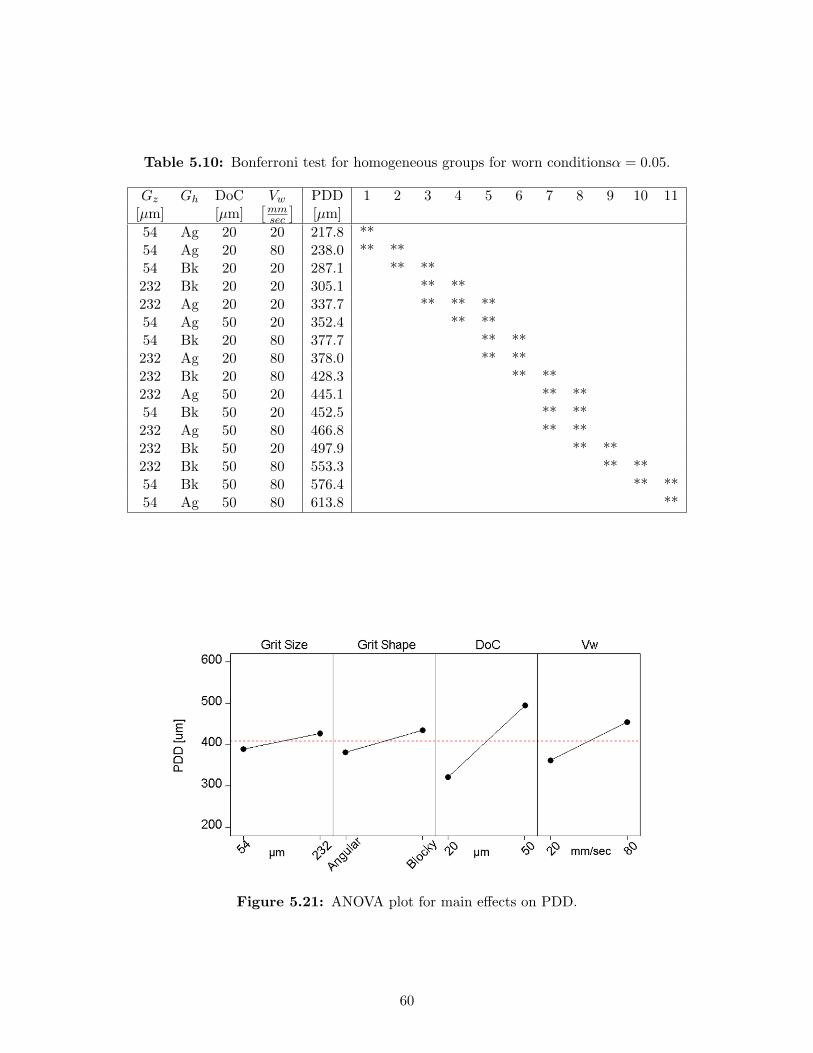
Table 5.10: Bonferroni test for homogeneous groups for worn conditionsα = 0.05.
Gz Gh DoC Vw PDD 1 2 3 4 5 6 7 8 9 10 11[µm] [µm]
[mmsec
][µm]
54 Ag 20 20 217.8 **54 Ag 20 80 238.0 ** **54 Bk 20 20 287.1 ** **232 Bk 20 20 305.1 ** **232 Ag 20 20 337.7 ** ** **54 Ag 50 20 352.4 ** **54 Bk 20 80 377.7 ** **232 Ag 20 80 378.0 ** **232 Bk 20 80 428.3 ** **232 Ag 50 20 445.1 ** **54 Bk 50 20 452.5 ** **232 Ag 50 80 466.8 ** **232 Bk 50 20 497.9 ** **232 Bk 50 80 553.3 ** **54 Bk 50 80 576.4 ** **54 Ag 50 80 613.8 **
Figure 5.21: ANOVA plot for main effects on PDD.
60
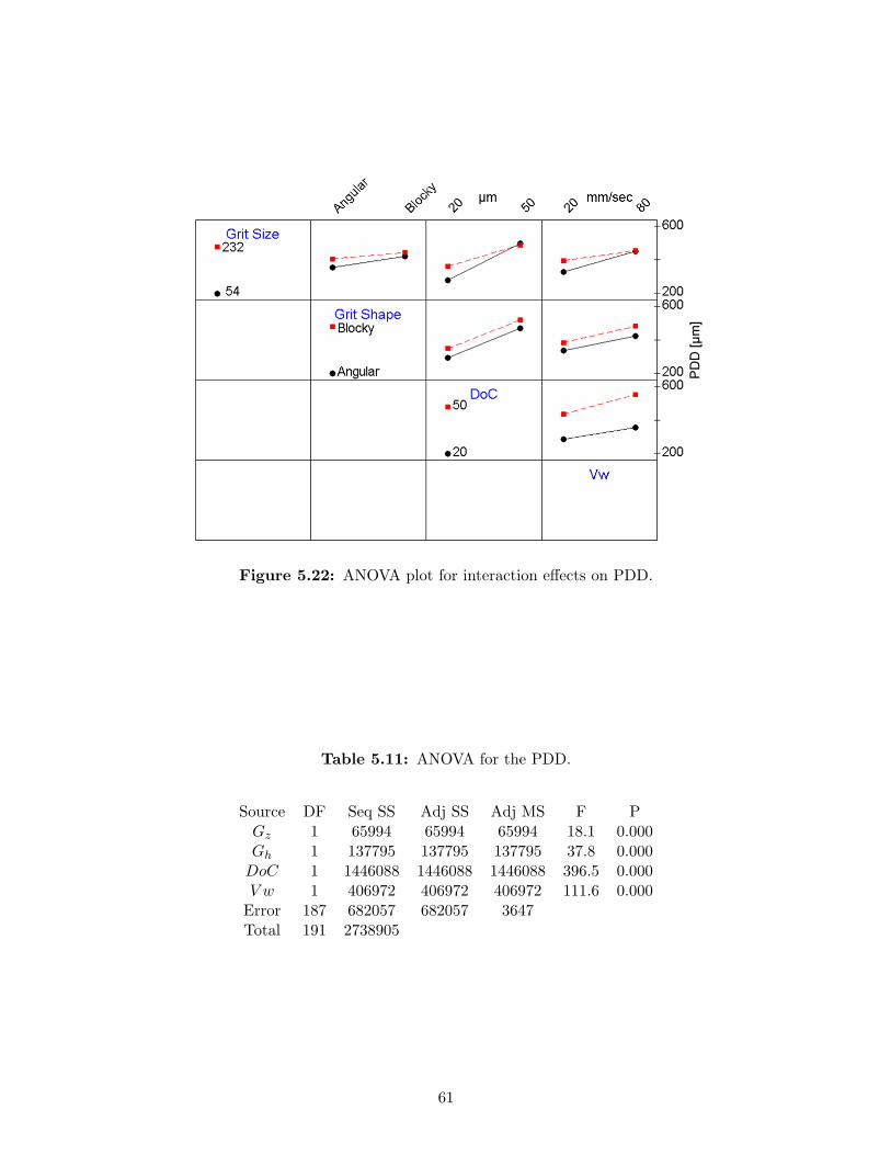
Figure 5.22: ANOVA plot for interaction effects on PDD.
Table 5.11: ANOVA for the PDD.
Source DF Seq SS Adj SS Adj MS F PGz 1 65994 65994 65994 18.1 0.000Gh 1 137795 137795 137795 37.8 0.000
DoC 1 1446088 1446088 1446088 396.5 0.000V w 1 406972 406972 406972 111.6 0.000
Error 187 682057 682057 3647Total 191 2738905
61
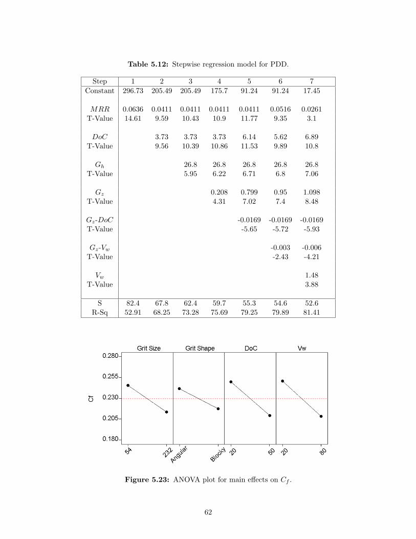
Table 5.12: Stepwise regression model for PDD.
Step 1 2 3 4 5 6 7Constant 296.73 205.49 205.49 175.7 91.24 91.24 17.45
MRR 0.0636 0.0411 0.0411 0.0411 0.0411 0.0516 0.0261T-Value 14.61 9.59 10.43 10.9 11.77 9.35 3.1
DoC 3.73 3.73 3.73 6.14 5.62 6.89T-Value 9.56 10.39 10.86 11.53 9.89 10.8
Gh 26.8 26.8 26.8 26.8 26.8T-Value 5.95 6.22 6.71 6.8 7.06
Gz 0.208 0.799 0.95 1.098T-Value 4.31 7.02 7.4 8.48
Gz-DoC -0.0169 -0.0169 -0.0169T-Value -5.65 -5.72 -5.93
Gz-Vw -0.003 -0.006T-Value -2.43 -4.21
Vw 1.48T-Value 3.88
S 82.4 67.8 62.4 59.7 55.3 54.6 52.6R-Sq 52.91 68.25 73.28 75.69 79.25 79.89 81.41
Figure 5.23: ANOVA plot for main effects on Cf .
62
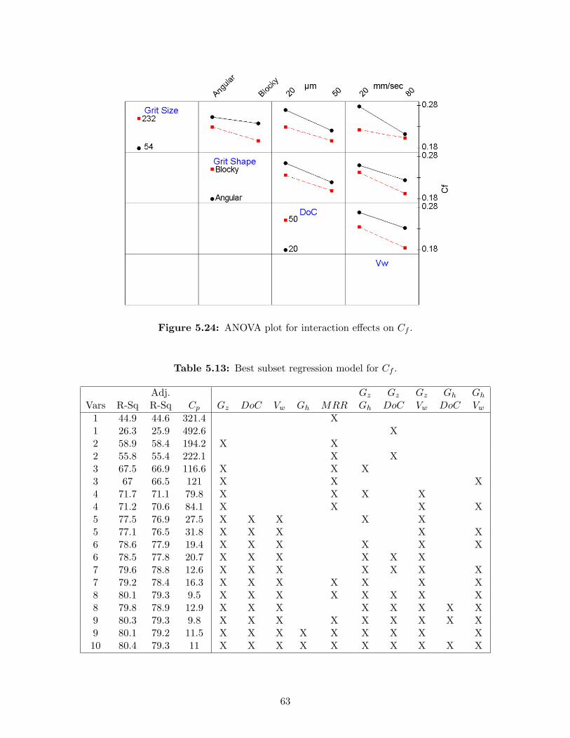
Figure 5.24: ANOVA plot for interaction effects on Cf .
Table 5.13: Best subset regression model for Cf .
Adj. Gz Gz Gz Gh Gh
Vars R-Sq R-Sq Cp Gz DoC Vw Gh MRR Gh DoC Vw DoC Vw
1 44.9 44.6 321.4 X1 26.3 25.9 492.6 X2 58.9 58.4 194.2 X X2 55.8 55.4 222.1 X X3 67.5 66.9 116.6 X X X3 67 66.5 121 X X X4 71.7 71.1 79.8 X X X X4 71.2 70.6 84.1 X X X X5 77.5 76.9 27.5 X X X X X5 77.1 76.5 31.8 X X X X X6 78.6 77.9 19.4 X X X X X X6 78.5 77.8 20.7 X X X X X X7 79.6 78.8 12.6 X X X X X X X7 79.2 78.4 16.3 X X X X X X X8 80.1 79.3 9.5 X X X X X X X X8 79.8 78.9 12.9 X X X X X X X X9 80.3 79.3 9.8 X X X X X X X X X9 80.1 79.2 11.5 X X X X X X X X X10 80.4 79.3 11 X X X X X X X X X X
63
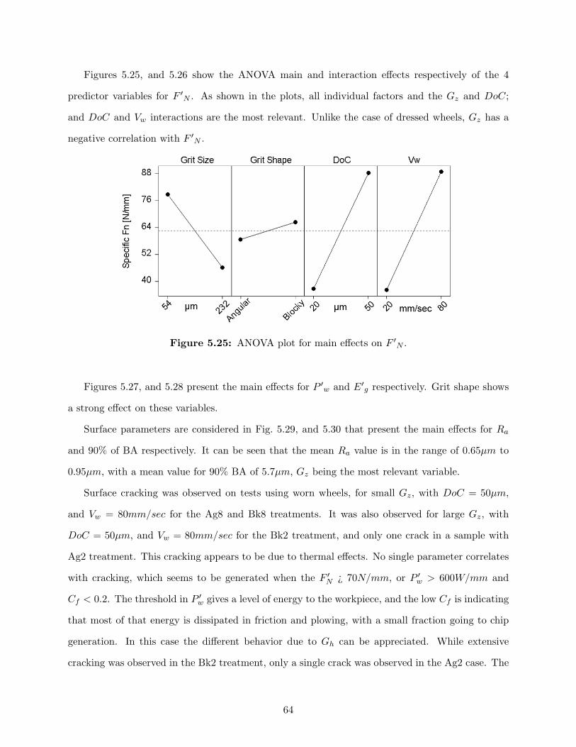
Figures 5.25, and 5.26 show the ANOVA main and interaction effects respectively of the 4
predictor variables for F ′N . As shown in the plots, all individual factors and the Gz and DoC;
and DoC and Vw interactions are the most relevant. Unlike the case of dressed wheels, Gz has a
negative correlation with F ′N .
Figure 5.25: ANOVA plot for main effects on F ′N .
Figures 5.27, and 5.28 present the main effects for P ′w and E′
g respectively. Grit shape shows
a strong effect on these variables.
Surface parameters are considered in Fig. 5.29, and 5.30 that present the main effects for Ra
and 90% of BA respectively. It can be seen that the mean Ra value is in the range of 0.65µm to
0.95µm, with a mean value for 90% BA of 5.7µm, Gz being the most relevant variable.
Surface cracking was observed on tests using worn wheels, for small Gz, with DoC = 50µm,
and Vw = 80mm/sec for the Ag8 and Bk8 treatments. It was also observed for large Gz, with
DoC = 50µm, and Vw = 80mm/sec for the Bk2 treatment, and only one crack in a sample with
Ag2 treatment. This cracking appears to be due to thermal effects. No single parameter correlates
with cracking, which seems to be generated when the F ′N ¿ 70N/mm, or P ′
w > 600W/mm and
Cf < 0.2. The threshold in P ′w gives a level of energy to the workpiece, and the low Cf is indicating
that most of that energy is dissipated in friction and plowing, with a small fraction going to chip
generation. In this case the different behavior due to Gh can be appreciated. While extensive
cracking was observed in the Bk2 treatment, only a single crack was observed in the Ag2 case. The
64
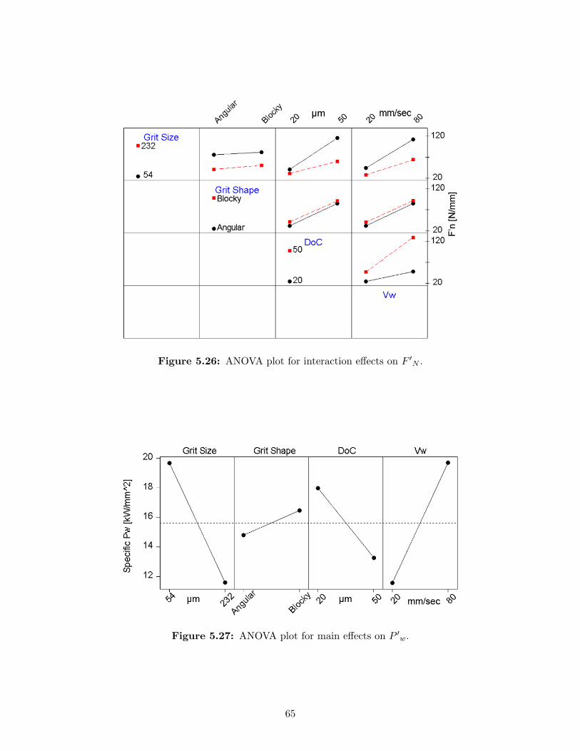
Figure 5.26: ANOVA plot for interaction effects on F ′N .
Figure 5.27: ANOVA plot for main effects on P ′w.
65
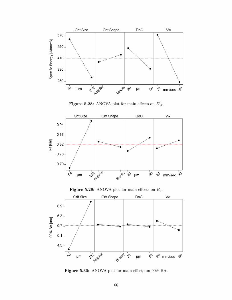
Figure 5.28: ANOVA plot for main effects on E′g.
Figure 5.29: ANOVA plot for main effects on Ra.
Figure 5.30: ANOVA plot for main effects on 90% BA.
66
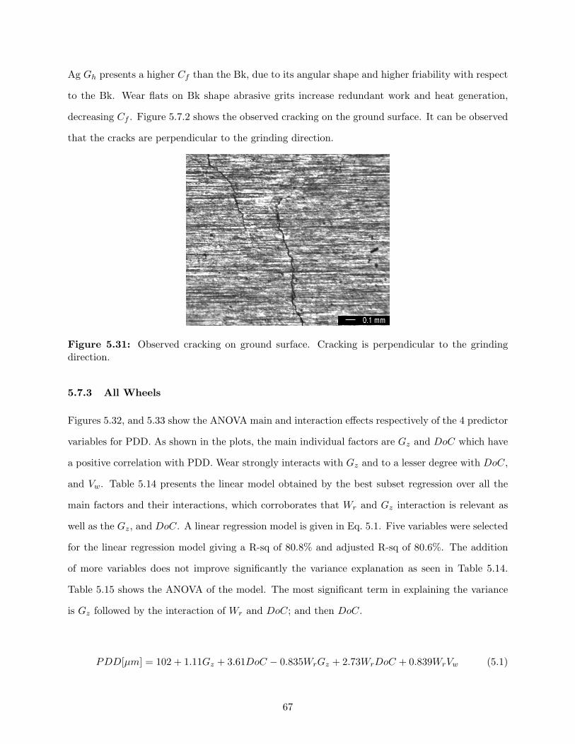
Ag Gh presents a higher Cf than the Bk, due to its angular shape and higher friability with respect
to the Bk. Wear flats on Bk shape abrasive grits increase redundant work and heat generation,
decreasing Cf . Figure 5.7.2 shows the observed cracking on the ground surface. It can be observed
that the cracks are perpendicular to the grinding direction.
Figure 5.31: Observed cracking on ground surface. Cracking is perpendicular to the grindingdirection.
5.7.3 All Wheels
Figures 5.32, and 5.33 show the ANOVA main and interaction effects respectively of the 4 predictor
variables for PDD. As shown in the plots, the main individual factors are Gz and DoC which have
a positive correlation with PDD. Wear strongly interacts with Gz and to a lesser degree with DoC,
and Vw. Table 5.14 presents the linear model obtained by the best subset regression over all the
main factors and their interactions, which corroborates that Wr and Gz interaction is relevant as
well as the Gz, and DoC. A linear regression model is given in Eq. 5.1. Five variables were selected
for the linear regression model giving a R-sq of 80.8% and adjusted R-sq of 80.6%. The addition
of more variables does not improve significantly the variance explanation as seen in Table 5.14.
Table 5.15 shows the ANOVA of the model. The most significant term in explaining the variance
is Gz followed by the interaction of Wr and DoC; and then DoC.
PDD[µm] = 102 + 1.11Gz + 3.61DoC − 0.835WrGz + 2.73WrDoC + 0.839WrVw (5.1)
67
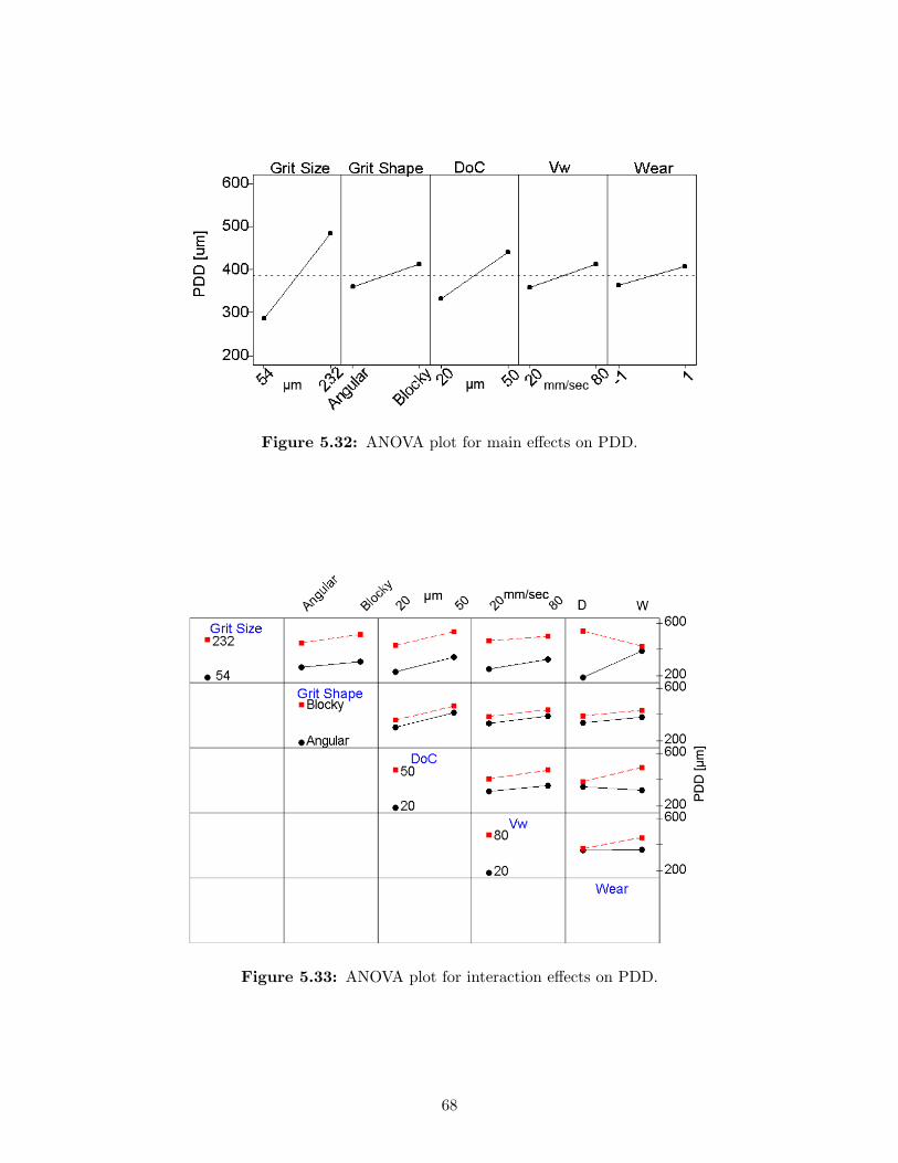
Figure 5.32: ANOVA plot for main effects on PDD.
Figure 5.33: ANOVA plot for interaction effects on PDD.
68
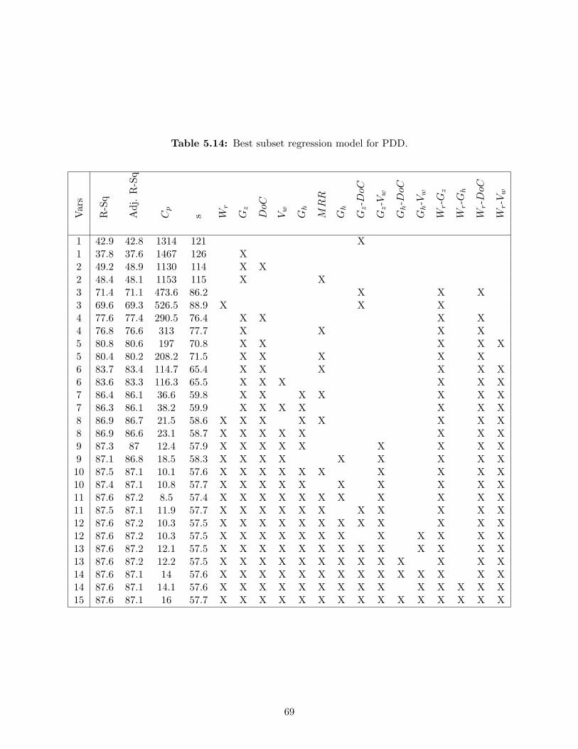
Table 5.14: Best subset regression model for PDD.
Var
s
R-S
q
Adj
.R
-Sq
Cp
s Wr
Gz
DoC
Vw
Gh
MR
R
Gh
Gz-D
oC
Gz-V
w
Gh-D
oC
Gh-V
w
Wr-G
z
Wr-G
h
Wr-D
oC
Wr-V
w
1 42.9 42.8 1314 121 X1 37.8 37.6 1467 126 X2 49.2 48.9 1130 114 X X2 48.4 48.1 1153 115 X X3 71.4 71.1 473.6 86.2 X X X3 69.6 69.3 526.5 88.9 X X X4 77.6 77.4 290.5 76.4 X X X X4 76.8 76.6 313 77.7 X X X X5 80.8 80.6 197 70.8 X X X X X5 80.4 80.2 208.2 71.5 X X X X X6 83.7 83.4 114.7 65.4 X X X X X X6 83.6 83.3 116.3 65.5 X X X X X X7 86.4 86.1 36.6 59.8 X X X X X X X7 86.3 86.1 38.2 59.9 X X X X X X X8 86.9 86.7 21.5 58.6 X X X X X X X X8 86.9 86.6 23.1 58.7 X X X X X X X X9 87.3 87 12.4 57.9 X X X X X X X X X9 87.1 86.8 18.5 58.3 X X X X X X X X X10 87.5 87.1 10.1 57.6 X X X X X X X X X X10 87.4 87.1 10.8 57.7 X X X X X X X X X X11 87.6 87.2 8.5 57.4 X X X X X X X X X X X11 87.5 87.1 11.9 57.7 X X X X X X X X X X X12 87.6 87.2 10.3 57.5 X X X X X X X X X X X X12 87.6 87.2 10.3 57.5 X X X X X X X X X X X X13 87.6 87.2 12.1 57.5 X X X X X X X X X X X X X13 87.6 87.2 12.2 57.5 X X X X X X X X X X X X X14 87.6 87.1 14 57.6 X X X X X X X X X X X X X X14 87.6 87.1 14.1 57.6 X X X X X X X X X X X X X X15 87.6 87.1 16 57.7 X X X X X X X X X X X X X X X
69
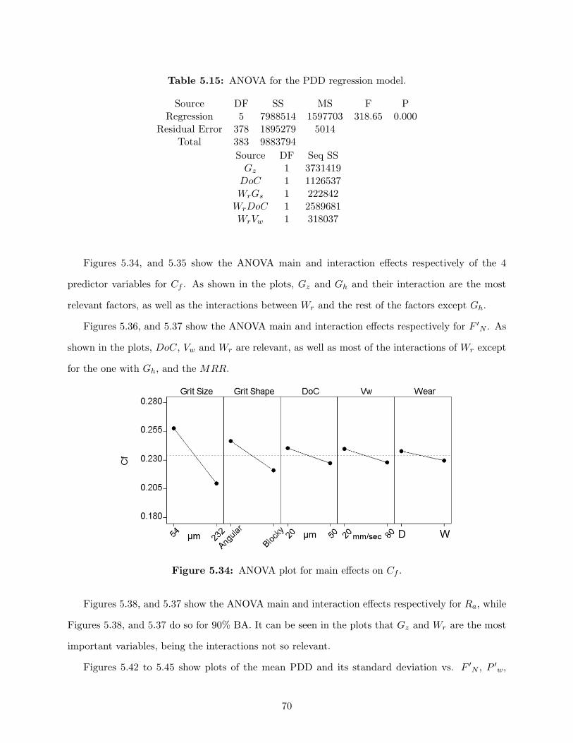
Table 5.15: ANOVA for the PDD regression model.
Source DF SS MS F PRegression 5 7988514 1597703 318.65 0.000
Residual Error 378 1895279 5014Total 383 9883794
Source DF Seq SSGz 1 3731419
DoC 1 1126537WrGs 1 222842
WrDoC 1 2589681WrVw 1 318037
Figures 5.34, and 5.35 show the ANOVA main and interaction effects respectively of the 4
predictor variables for Cf . As shown in the plots, Gz and Gh and their interaction are the most
relevant factors, as well as the interactions between Wr and the rest of the factors except Gh.
Figures 5.36, and 5.37 show the ANOVA main and interaction effects respectively for F ′N . As
shown in the plots, DoC, Vw and Wr are relevant, as well as most of the interactions of Wr except
for the one with Gh, and the MRR.
Figure 5.34: ANOVA plot for main effects on Cf .
Figures 5.38, and 5.37 show the ANOVA main and interaction effects respectively for Ra, while
Figures 5.38, and 5.37 do so for 90% BA. It can be seen in the plots that Gz and Wr are the most
important variables, being the interactions not so relevant.
Figures 5.42 to 5.45 show plots of the mean PDD and its standard deviation vs. F ′N , P ′
w,
70
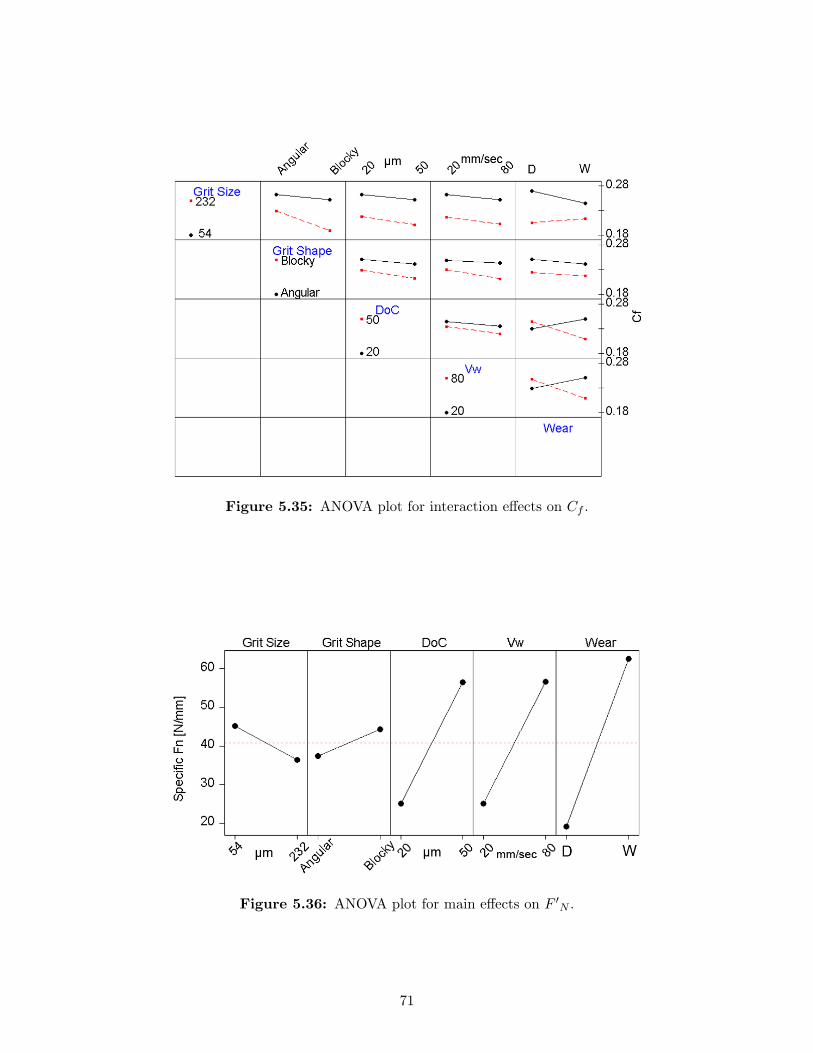
Figure 5.35: ANOVA plot for interaction effects on Cf .
Figure 5.36: ANOVA plot for main effects on F ′N .
71
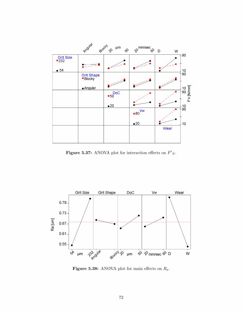
Figure 5.37: ANOVA plot for interaction effects on F ′N .
Figure 5.38: ANOVA plot for main effects on Ra.
72
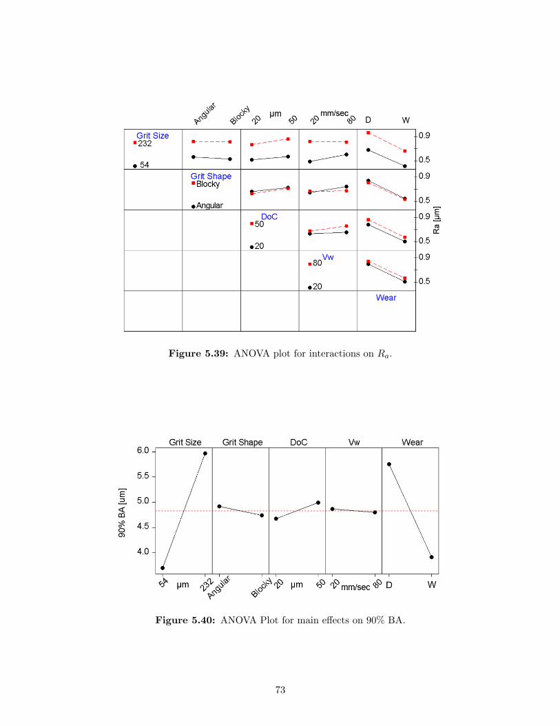
Figure 5.39: ANOVA plot for interactions on Ra.
Figure 5.40: ANOVA Plot for main effects on 90% BA.
73
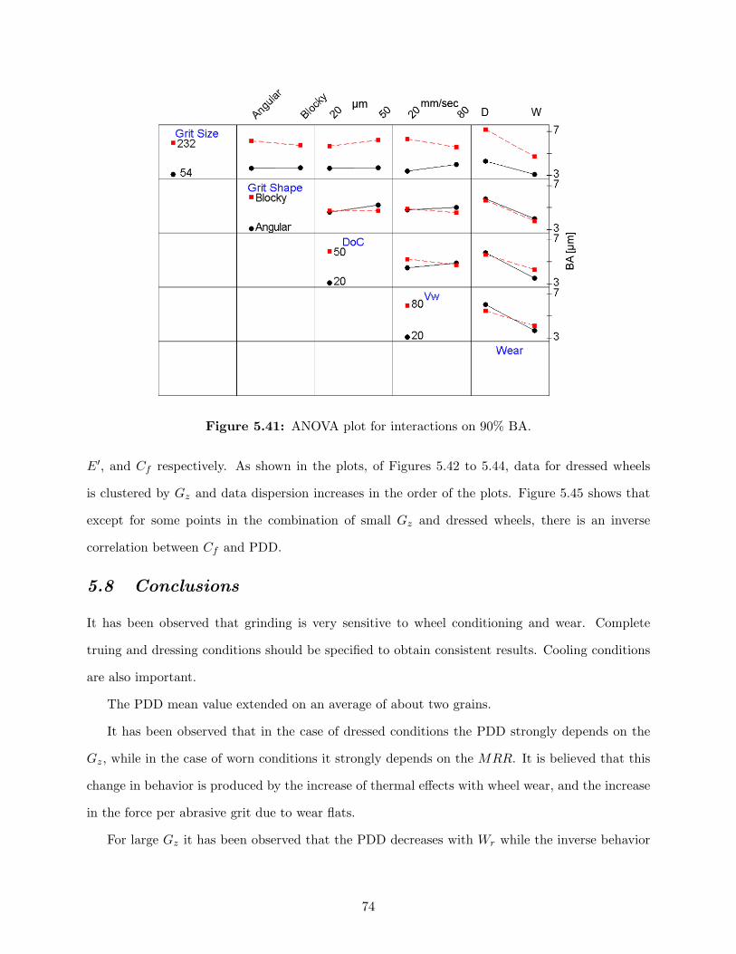
Figure 5.41: ANOVA plot for interactions on 90% BA.
E′, and Cf respectively. As shown in the plots, of Figures 5.42 to 5.44, data for dressed wheels
is clustered by Gz and data dispersion increases in the order of the plots. Figure 5.45 shows that
except for some points in the combination of small Gz and dressed wheels, there is an inverse
correlation between Cf and PDD.
5.8 Conclusions
It has been observed that grinding is very sensitive to wheel conditioning and wear. Complete
truing and dressing conditions should be specified to obtain consistent results. Cooling conditions
are also important.
The PDD mean value extended on an average of about two grains.
It has been observed that in the case of dressed conditions the PDD strongly depends on the
Gz, while in the case of worn conditions it strongly depends on the MRR. It is believed that this
change in behavior is produced by the increase of thermal effects with wheel wear, and the increase
in the force per abrasive grit due to wear flats.
For large Gz it has been observed that the PDD decreases with Wr while the inverse behavior
74
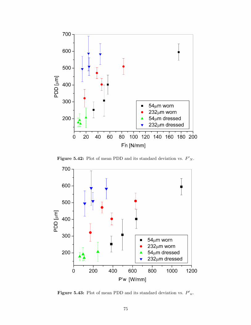
Figure 5.42: Plot of mean PDD and its standard deviation vs. F ′N .
Figure 5.43: Plot of mean PDD and its standard deviation vs. P ′w.
75
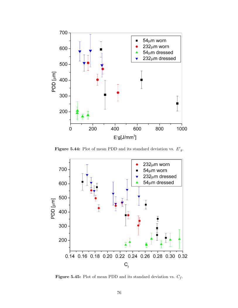
Figure 5.44: Plot of mean PDD and its standard deviation vs. E′g.
Figure 5.45: Plot of mean PDD and its standard deviation vs. Cf .
76
was observed for small Gz. While the P ′w was of the same order of magnitude for large Gz in
the cases of worn and dressed conditions, it increased an average of 6 times for small Gz. This
would indicate that in the case of large Gz the thermal effects were not very different for the two Wr
conditions and the PDD was determined by the Gz. The decrease of the PDD could be explained by
assuming that the worn wheel presented a narrower distribution of cutting edges than the dressed
one. This could be due to some fracture of the abrasive grits during the first stages of grinding
after dressing, resulting as if having a smaller grit size. In the case of small Gz can be assumed
that the generation of wear flats increased the force per abrasive grit and temperature with the
consequent increase of the PDD.
It has been observed that the PDD is inversely correlated to the Cf .
No cracking was observed on the ground surface under a magnification of 60X for dressed
wheels.
Surface cracking was observed on tests using worn wheels for small Gz in the 4 treatments with
the largest MRR. This cracking appears to be due to thermal effects and it was not related to the
PDD. It has been observed that cracking was produced on treatments with high F ′N , or high P ′
w
and low Cf .
It was observed that the Ra and BA mean values increased with wear. This was probably due
to the effect of plowing in the formation of side ridges.
5.8.1 PDD
The PDD mean value was of the order of ' 400µm with an observed minimum and maximum
of ' 100µm and ' 800µm respectively. Considering that the lamellae size was of the order of
' 250µm, the measured PDD extends on an average of about two grains.
In the case of dressed wheels the PDD measured for small Gz statistically lies in the same range,
as well as several groups of treatments for large Gz. The PDD mean and standard deviation for
small and large Gz are 186± 40µm, and 543± 85µm respectively.
Most of the PDD variance can be explained by the Gz factor alone, Vw being not a relevant
factor. There is some influence of the Gh, and the interactions between Gz and Gh; and Gz and
DoC. The R-Sq value for the model PDD[µm] = 78.1 + 2.007GS is 87.9%.
77
In the case of worn wheels, unlike the case of dressed wheels, there is no unique factor that
dominates PDD. The main factors are DoC and Vw which have positive correlation with PDD,
therefore MRR also has a positive correlation with PDD. Grit size and shape are not so relevant
in this case. The DoC explains half of the data variance followed in importance by Vw. Even
considering most of the controlled variables and their interaction in a linear model, the R-Sq value
is less than 0.82. The PDD mean and standard deviation was of 407± 120µm for worn wheels and
365± 191µm for dressed ones
An R-sq value of 0.84 is obtained by a linear fit of PDD with Cf .
5.8.2 Grinding Friction Coefficient
Grit size and shape have a negative correlation with Cf , while the correlation with DoC and Vw is
positive. In the case of worn wheels all individual factors, and the interactions between Gz and the
rest of the variables are relevant for Cf , and their correlation is inverse to the one shown for PDD.
While the Cf trend with Gz and Gh is the same as with dressed wheels, the dependence on DoC,
and Vw is inverse. The negative correlation of the the Cf with DoC and Vw can be explained by
considering the shape change in the abrasives.
5.8.3 Specific Normal Force
In the case of dressed wheels, F ′N has a positive correlation with all the individual factors, and the
Gz and Gh interaction.
In the case of dressed wheels, all individual factors and the Gz and DoC; and DoC and Vw
interactions are relevant for F ′N . Unlike the case of dressed wheels, Gz has a negative correlation
with F ′N , which can be explained by assuming that the relative wear flat in the small grit is larger
than in the large grit. This can be due to the fact that poorer lubrication conditions might occur
with smaller grits, with higher temperatures, and increased wear rate of the diamond.
5.8.4 Surface Parameters
For the dressed conditions, the mean Ra value is in the range of 0.4µm to 0.7µm, and the mean
90% BA of 3.9µm, Gz being is the most relevant factor.
78
For the worn conditions, the mean Ra value is in the range of 0.65µm to 0.95µm, with a mean
value for 90% BA of 5.7µm, Gz being the most relevant variable.
The Ra mean value increased ' 0.25µm from the dressed wheel condition to the worn one, and a
similar trend was observed for BA. Worn wheels have a narrower spatial cutting edges distribution
than in dressed conditions, also the chip thickness is smaller. Therefore, a possible explanation for
the increase in roughness is the plowing increase with the formation of scratching side ridges.
5.8.5 Cracking
Surface cracking was observed on tests using worn wheels, for small Gz, with DoC = 50µm, and
Vw = 80mm/sec for the Ag8 and Bk8 treatments. It was also observed in the case of large Gz,
with DoC = 50µm, and Vw = 80mm/sec for the Bk2 treatment, and only one crack in a sample
with Ag2 treatment. This cracking appears to be due to thermal effects. Cracking seems to be
generated when the F ′N ¿ 70N/mm, or P ′
w > 600W/mm and Cf < 0.2. The threshold in P ′w
gives a level of energy to the workpiece, and the low Cf is indicating that most of that energy is
dissipated in friction and plowing, with a small fraction going to chip generation. In this case the
different behavior due to Gh can be appreciated. While extensive cracking was observed in the Bk2
treatment, only a single crack was observed in the Ag2 case. The Ag Gh presents a higher Cf than
the Bk, due to its angular shape and higher friability with respect to the Bk. Wear flats on Bk
shape abrasive grits increase redundant work and heat generation, decreasing Cf .
79
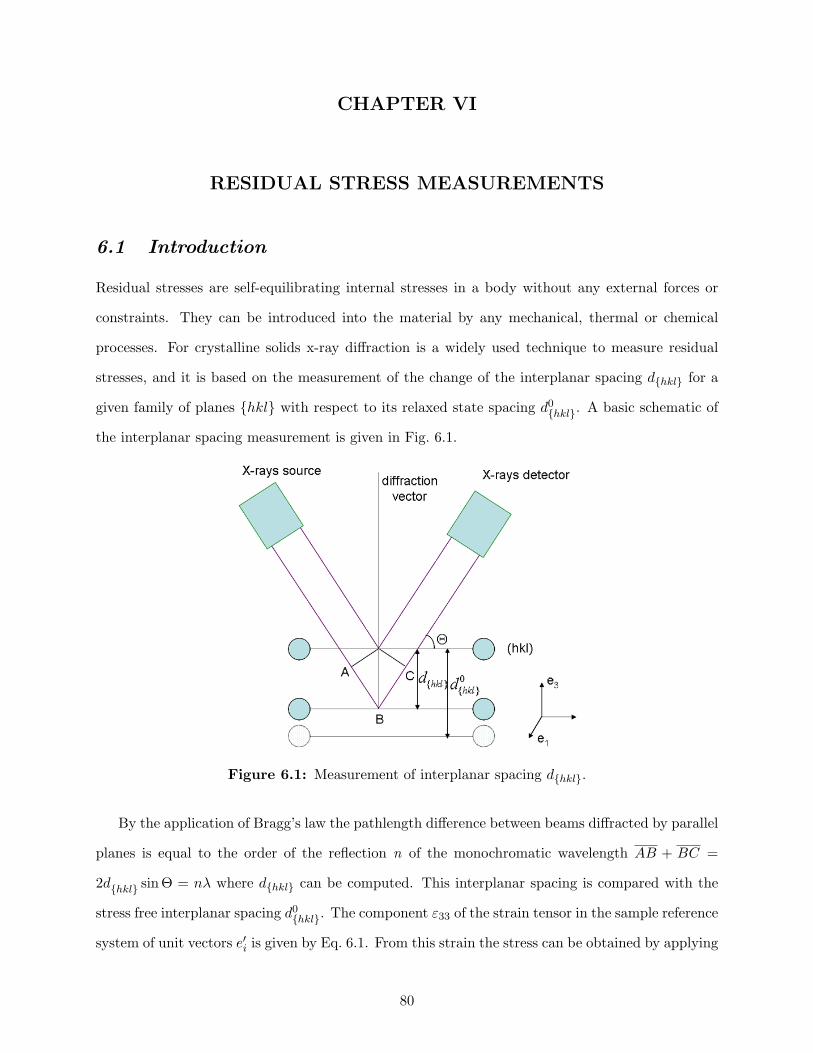
CHAPTER VI
RESIDUAL STRESS MEASUREMENTS
6.1 Introduction
Residual stresses are self-equilibrating internal stresses in a body without any external forces or
constraints. They can be introduced into the material by any mechanical, thermal or chemical
processes. For crystalline solids x-ray diffraction is a widely used technique to measure residual
stresses, and it is based on the measurement of the change of the interplanar spacing dhkl for a
given family of planes hkl with respect to its relaxed state spacing d0hkl. A basic schematic of
the interplanar spacing measurement is given in Fig. 6.1.
Figure 6.1: Measurement of interplanar spacing dhkl.
By the application of Bragg’s law the pathlength difference between beams diffracted by parallel
planes is equal to the order of the reflection n of the monochromatic wavelength AB + BC =
2dhkl sinΘ = nλ where dhkl can be computed. This interplanar spacing is compared with the
stress free interplanar spacing d0hkl. The component ε33 of the strain tensor in the sample reference
system of unit vectors e′i is given by Eq. 6.1. From this strain the stress can be obtained by applying
80
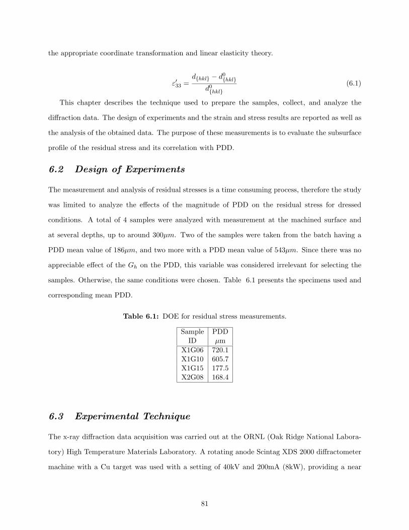
the appropriate coordinate transformation and linear elasticity theory.
ε′33 =dhkl − d0
hkl
d0hkl
(6.1)
This chapter describes the technique used to prepare the samples, collect, and analyze the
diffraction data. The design of experiments and the strain and stress results are reported as well as
the analysis of the obtained data. The purpose of these measurements is to evaluate the subsurface
profile of the residual stress and its correlation with PDD.
6.2 Design of Experiments
The measurement and analysis of residual stresses is a time consuming process, therefore the study
was limited to analyze the effects of the magnitude of PDD on the residual stress for dressed
conditions. A total of 4 samples were analyzed with measurement at the machined surface and
at several depths, up to around 300µm. Two of the samples were taken from the batch having a
PDD mean value of 186µm, and two more with a PDD mean value of 543µm. Since there was no
appreciable effect of the Gh on the PDD, this variable was considered irrelevant for selecting the
samples. Otherwise, the same conditions were chosen. Table 6.1 presents the specimens used and
corresponding mean PDD.
Table 6.1: DOE for residual stress measurements.
Sample PDDID µm
X1G06 720.1X1G10 605.7X1G15 177.5X2G08 168.4
6.3 Experimental Technique
The x-ray diffraction data acquisition was carried out at the ORNL (Oak Ridge National Labora-
tory) High Temperature Materials Laboratory. A rotating anode Scintag XDS 2000 diffractometer
machine with a Cu target was used with a setting of 40kV and 200mA (8kW), providing a near
81
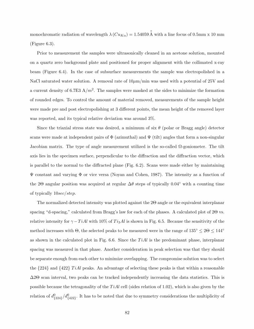
monochromatic radiation of wavelength λ (CuKα) = 1.54059A with a line focus of 0.5mm x 10 mm
(Figure 6.3).
Prior to measurement the samples were ultrasonically cleaned in an acetone solution, mounted
on a quartz zero background plate and positioned for proper alignment with the collimated x-ray
beam (Figure 6.4). In the case of subsurface measurements the sample was electropolished in a
NaCl saturated water solution. A removal rate of 10µm/min was used with a potential of 25V and
a current density of 6.7E3 A/m2. The samples were masked at the sides to minimize the formation
of rounded edges. To control the amount of material removed, measurements of the sample height
were made pre and post electropolishing at 3 different points, the mean height of the removed layer
was reported, and its typical relative deviation was around 3%.
Since the triaxial stress state was desired, a minimum of six θ (polar or Bragg angle) detector
scans were made at independent pairs of Φ (azimuthal) and Ψ (tilt) angles that form a non-singular
Jacobian matrix. The type of angle measurement utilized is the so-called Ω-goniometer. The tilt
axis lies in the specimen surface, perpendicular to the diffraction and the diffraction vector, which
is parallel to the normal to the diffracted plane (Fig. 6.2). Scans were made either by maintaining
Ψ constant and varying Φ or vice versa (Noyan and Cohen, 1987). The intensity as a function of
the 2Θ angular position was acquired at regular ∆θ steps of typically 0.04 with a counting time
of typically 10sec/step.
The normalized detected intensity was plotted against the 2Θ angle or the equivalent interplanar
spacing “d-spacing,” calculated from Bragg’s law for each of the phases. A calculated plot of 2Θ vs.
relative intensity for γ−TiAl with 10% of Ti3Al is shown in Fig. 6.5. Because the sensitivity of the
method increases with Θ, the selected peaks to be measured were in the range of 135 ≤ 2Θ ≤ 144
as shown in the calculated plot in Fig. 6.6. Since the TiAl is the predominant phase, interplanar
spacing was measured in that phase. Another consideration in peak selection was that they should
be separate enough from each other to minimize overlapping. The compromise solution was to select
the 224 and 422 TiAl peaks. An advantage of selecting these peaks is that within a reasonable
∆2Θ scan interval, two peaks can be tracked independently increasing the data statistics. This is
possible because the tetragonality of the TiAl cell (sides relation of 1.02), which is also given by the
relation of d0224/d0
422. It has to be noted that due to symmetry considerations the multiplicity of
82
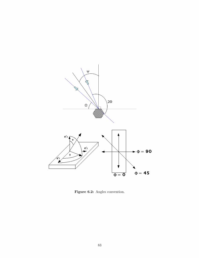
Figure 6.2: Angles convention.
83
the d224 family of planes is of 8 while the d422 is of 16, having their peaks a theoretical intensity
relation of ri = 3.0/6.4.
Figure 6.7 presents an experimental plot of the normalized intensity in CPS (counts per second)
vs. 2Θ. The 224 and 422 peaks can be clearly seen and are composed by the doublet Kα1
and Kα2 radiation from the Cu target. The standard approach (Ely et al., 1999) is to separate the
total intensity as composed by the intensity of the peak, in this case a doublet, and the background
contribution (Eq. 6.2).
I2Θ = Ipeak[shape function] + [background]
(shape function)doublet = (shape function)Kα1+ (shape function)Kα2
(6.2)
Where I2Θ is the intensity at the specified angle 2Θ and the shape function can be one of several
standard functions (Gaussian, pseudo Voigt, Pearson-VII, etc.). Typically, the shape function is
defined so that it varies in magnitude between 0 and 1 hence, the need for the scale parameter Ipeak
in Eq. 6.2 to adjust the fitting function to the same vertical scale as that of the data. Prior to the
data fit, the background energy was subtracted assuming a linear dependence with 2Θ. All four
peaks were fitted together to the Pearson-VII function considering least-squares error minimization.
Figure 6.7 shows the partial fits and the total fit which is a good approximation to the acquired
data. The value of the dhkl spacing was obtained from the 2Θ at maximum intensity of the
respective Kα1 peak using Bragg’s law. In theory each peak should be a Dirac delta function at
the theoretical dhkl value. In practice this is not possible. Factors such as the fact that radiation
is not monochromatic, and dhkl spacing is not constant in the irradiated volume widen the peak.
Therefore, there is an associated indetermination on the position of the peak maximum which will
be propagated to the final residual stress.
Accurate lattice strain can only be determined if the irradiated area of the specimen has a
sufficient number of randomly oriented grains of the phase of interest. This condition is not fulfilled
in coarse grained material as in this case. To improve this situation, the specimen was mounted
on a reciprocating stage which was moving in the range of ±5mm during the acquisition, enlarging
the irradiated area.
Another important issue is to determine d0hkl since the analysis is very sensitive to this value.
84
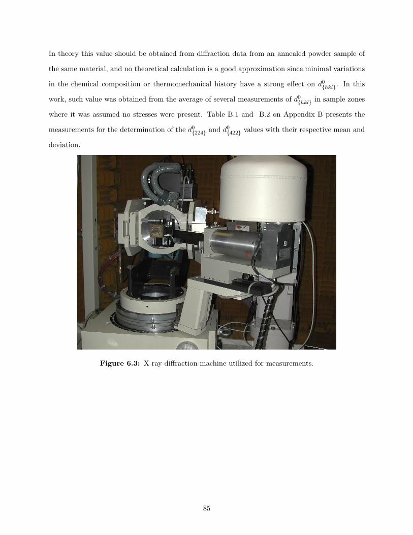
In theory this value should be obtained from diffraction data from an annealed powder sample of
the same material, and no theoretical calculation is a good approximation since minimal variations
in the chemical composition or thermomechanical history have a strong effect on d0hkl. In this
work, such value was obtained from the average of several measurements of d0hkl in sample zones
where it was assumed no stresses were present. Table B.1 and B.2 on Appendix B presents the
measurements for the determination of the d0224 and d0
422 values with their respective mean and
deviation.
Figure 6.3: X-ray diffraction machine utilized for measurements.
85
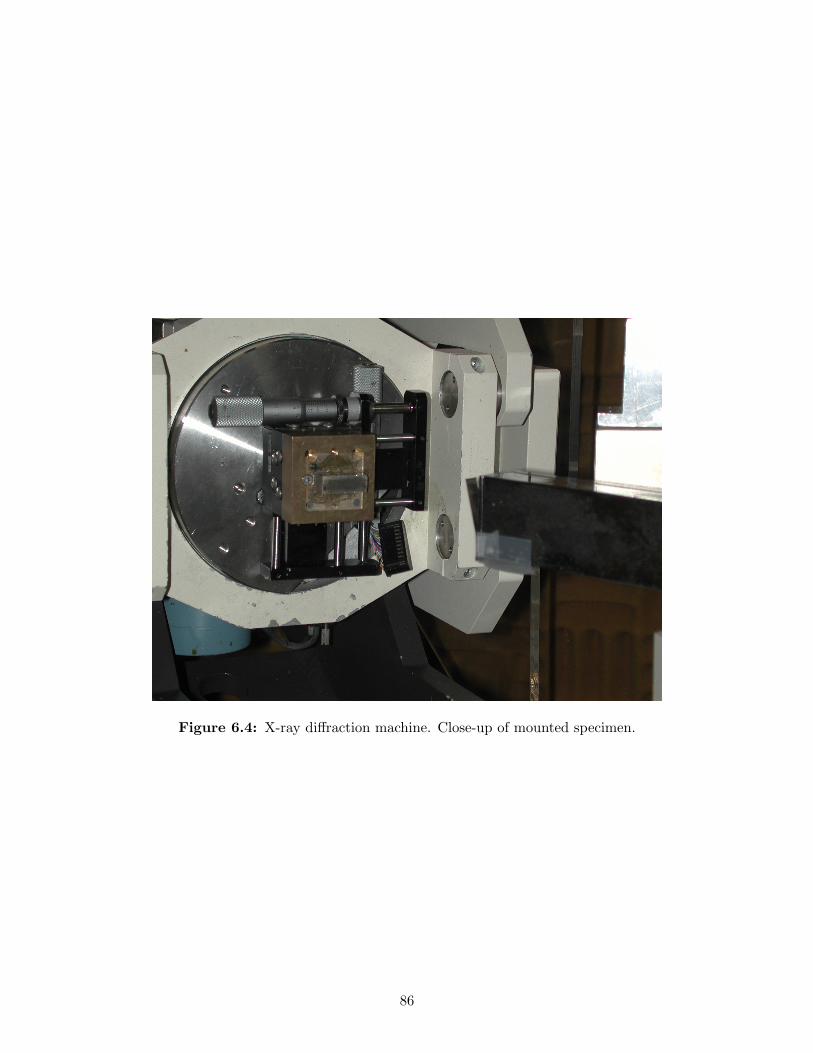
Figure 6.4: X-ray diffraction machine. Close-up of mounted specimen.
86
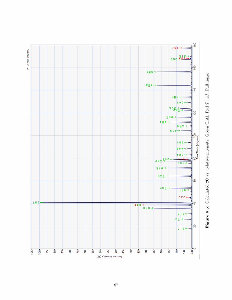
Fig
ure
6.5:
Cal
cula
ted
2Θvs
.re
lati
vein
tens
ity.
Gre
enT
iAl.
Red
Ti 3
Al.
Full
rang
e.
87
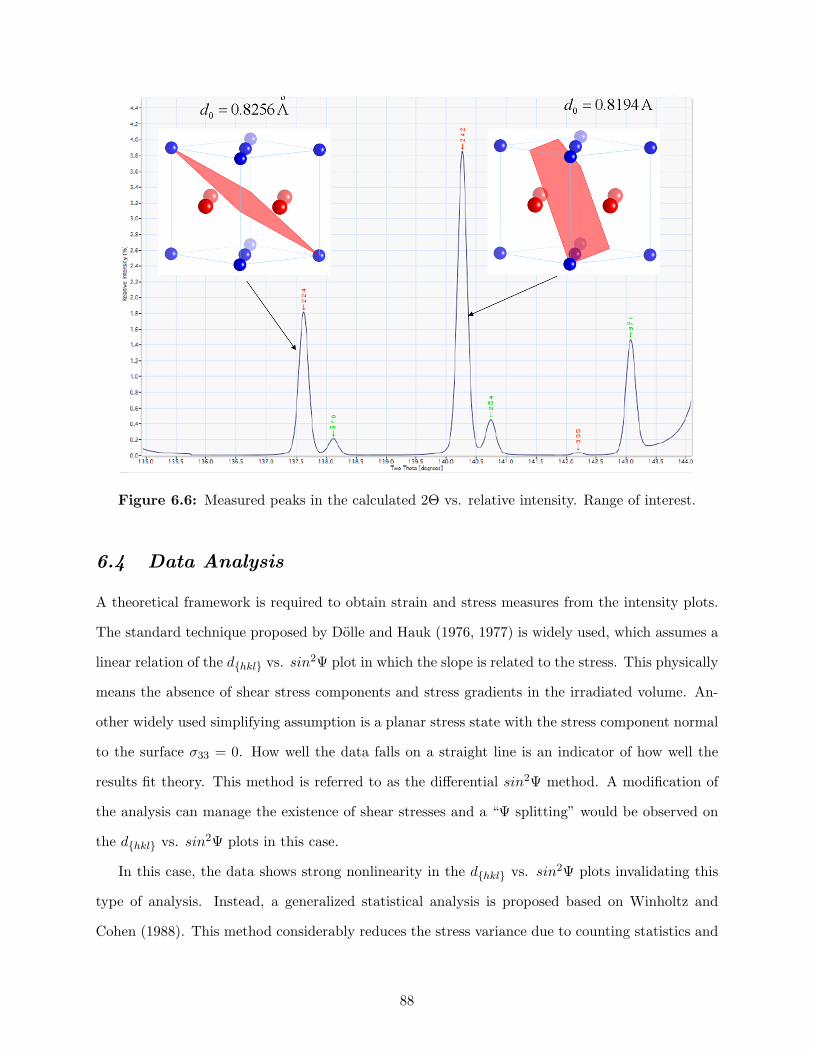
Figure 6.6: Measured peaks in the calculated 2Θ vs. relative intensity. Range of interest.
6.4 Data Analysis
A theoretical framework is required to obtain strain and stress measures from the intensity plots.
The standard technique proposed by Dolle and Hauk (1976, 1977) is widely used, which assumes a
linear relation of the dhkl vs. sin2Ψ plot in which the slope is related to the stress. This physically
means the absence of shear stress components and stress gradients in the irradiated volume. An-
other widely used simplifying assumption is a planar stress state with the stress component normal
to the surface σ33 = 0. How well the data falls on a straight line is an indicator of how well the
results fit theory. This method is referred to as the differential sin2Ψ method. A modification of
the analysis can manage the existence of shear stresses and a “Ψ splitting” would be observed on
the dhkl vs. sin2Ψ plots in this case.
In this case, the data shows strong nonlinearity in the dhkl vs. sin2Ψ plots invalidating this
type of analysis. Instead, a generalized statistical analysis is proposed based on Winholtz and
Cohen (1988). This method considerably reduces the stress variance due to counting statistics and
88
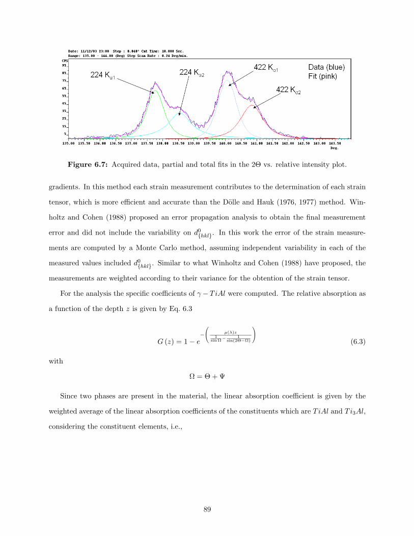
Figure 6.7: Acquired data, partial and total fits in the 2Θ vs. relative intensity plot.
gradients. In this method each strain measurement contributes to the determination of each strain
tensor, which is more efficient and accurate than the Dolle and Hauk (1976, 1977) method. Win-
holtz and Cohen (1988) proposed an error propagation analysis to obtain the final measurement
error and did not include the variability on d0hkl. In this work the error of the strain measure-
ments are computed by a Monte Carlo method, assuming independent variability in each of the
measured values included d0hkl. Similar to what Winholtz and Cohen (1988) have proposed, the
measurements are weighted according to their variance for the obtention of the strain tensor.
For the analysis the specific coefficients of γ− TiAl were computed. The relative absorption as
a function of the depth z is given by Eq. 6.3
G (z) = 1− e−(
µ(λ)z1
sin Ω− 1
sin(2Θ−Ω)
)(6.3)
with
Ω = Θ + Ψ
Since two phases are present in the material, the linear absorption coefficient is given by the
weighted average of the linear absorption coefficients of the constituents which are TiAl and Ti3Al,
considering the constituent elements, i.e.,
89
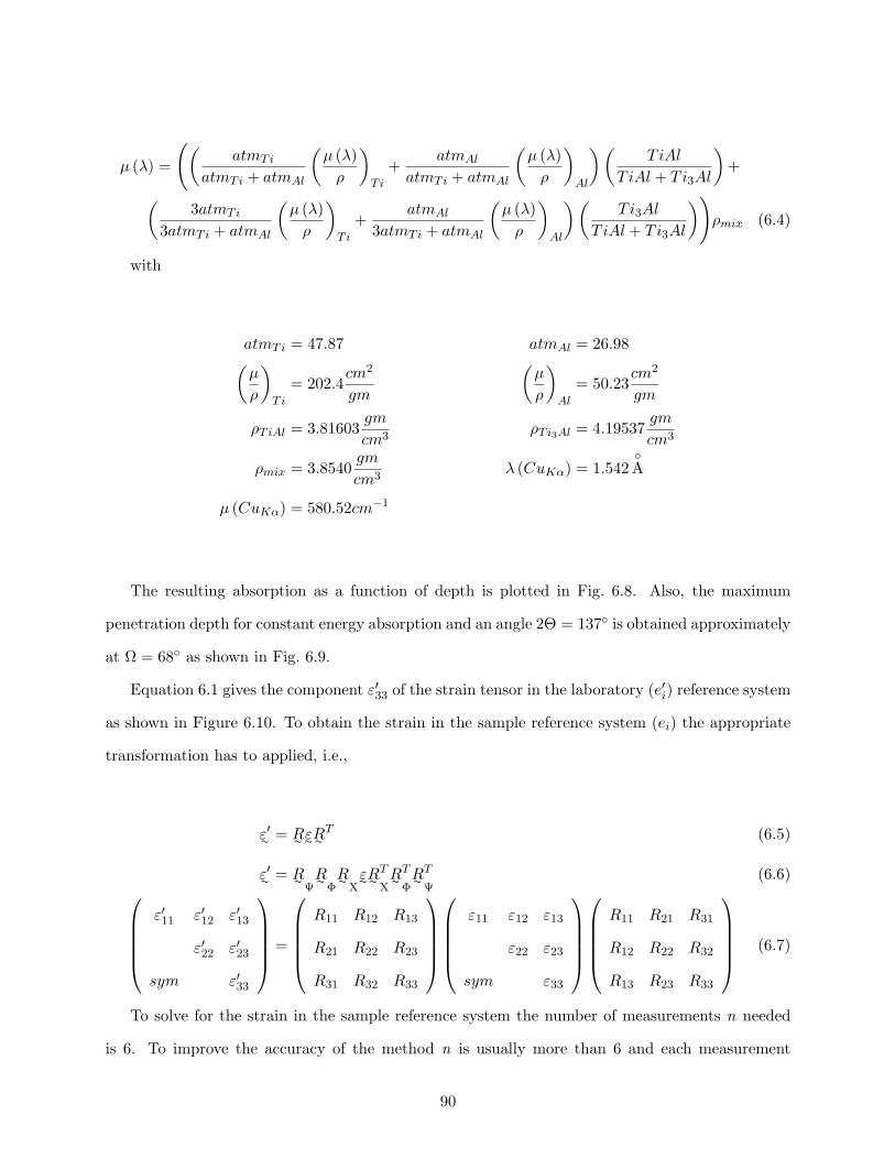
µ (λ) =
((atmTi
atmTi + atmAl
(µ (λ)
ρ
)Ti
+atmAl
atmTi + atmAl
(µ (λ)
ρ
)Al
)(TiAl
T iAl + Ti3Al
)+
(3atmTi
3atmTi + atmAl
(µ (λ)
ρ
)Ti
+atmAl
3atmTi + atmAl
(µ (λ)
ρ
)Al
)(Ti3Al
T iAl + Ti3Al
))ρmix (6.4)
with
atmTi = 47.87 atmAl = 26.98(µ
ρ
)Ti
= 202.4cm2
gm
(µ
ρ
)Al
= 50.23cm2
gm
ρTiAl = 3.81603gm
cm3ρTi3Al = 4.19537
gm
cm3
ρmix = 3.8540gm
cm3λ (CuKα) = 1.542
A
µ (CuKα) = 580.52cm−1
The resulting absorption as a function of depth is plotted in Fig. 6.8. Also, the maximum
penetration depth for constant energy absorption and an angle 2Θ = 137 is obtained approximately
at Ω = 68 as shown in Fig. 6.9.
Equation 6.1 gives the component ε′33 of the strain tensor in the laboratory (e′i) reference system
as shown in Figure 6.10. To obtain the strain in the sample reference system (ei) the appropriate
transformation has to applied, i.e.,
ε′∼ = R∼ ε∼R∼T (6.5)
ε′∼ = R∼ΨR∼
ΦR∼
Xε∼R∼
T
XR∼
T
ΦR∼
T
Ψ(6.6)
ε′11 ε′12 ε′13
ε′22 ε′23
sym ε′33
=
R11 R12 R13
R21 R22 R23
R31 R32 R33
ε11 ε12 ε13
ε22 ε23
sym ε33
R11 R21 R31
R12 R22 R32
R13 R23 R33
(6.7)
To solve for the strain in the sample reference system the number of measurements n needed
is 6. To improve the accuracy of the method n is usually more than 6 and each measurement
90
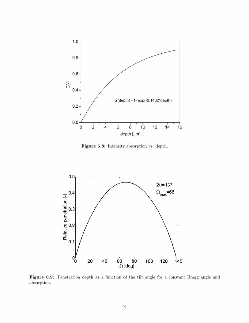
Figure 6.8: Intensity absorption vs. depth.
Figure 6.9: Penetration depth as a function of the tilt angle for a constant Bragg angle andabsorption.
91
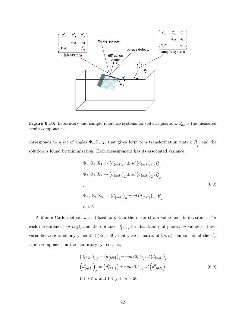
Figure 6.10: Laboratory and sample reference systems for data acquisition. ε′33 is the measuredstrain component.
corresponds to a set of angles Ψi,Φi, χi that gives form to a transformation matrix R∼i, and the
solution is found by minimization. Each measurement has its associated variance:
Ψ1,Φ1,X1 →(dhkl
)1± sd
(dhkl
)1, R∼
1
Ψ2,Φ2,X2 →(dhkl
)2± sd
(dhkl
)2, R∼
2
...
Ψn,Φn,Xn →(dhkl
)n± sd
(dhkl
)n
, R∼n
n > 6
(6.8)
A Monte Carlo method was utilized to obtain the mean strain value and its deviation. For
each measurement (dhkl)i and the obtained d0hkl for that family of planes, m values of these
variables were randomly generated (Eq. 6.9), that gave a matrix of [m,n] components of the ε′33
strain component on the laboratory system, i.e.,
(dhkl
)i,j
=(dhkl
)i± rnd (0, 1)j sd
(dhkl
)i(
d0hkl
)j
=(d0hkl
)± rnd (0, 1)j sd
(d0hkl
)1 6 i 6 n and 1 6 j 6 m = 20
(6.9)
92
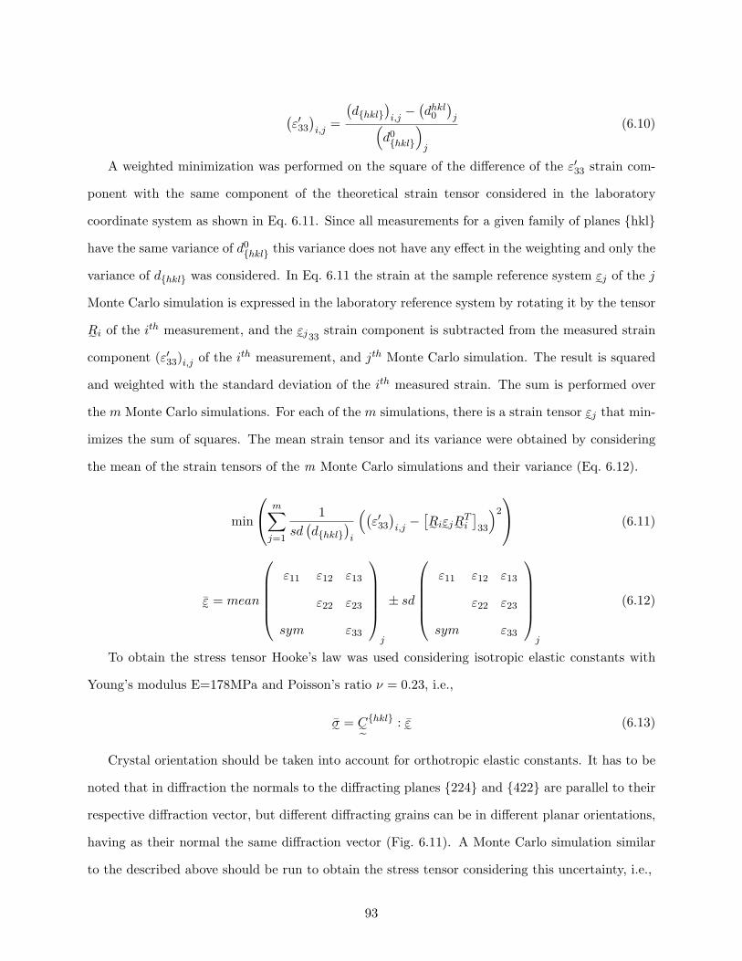
(ε′33
)i,j
=
(dhkl
)i,j−(dhkl
0
)j(
d0hkl
)j
(6.10)
A weighted minimization was performed on the square of the difference of the ε′33 strain com-
ponent with the same component of the theoretical strain tensor considered in the laboratory
coordinate system as shown in Eq. 6.11. Since all measurements for a given family of planes hkl
have the same variance of d0hkl this variance does not have any effect in the weighting and only the
variance of dhkl was considered. In Eq. 6.11 the strain at the sample reference system ε˜j of the j
Monte Carlo simulation is expressed in the laboratory reference system by rotating it by the tensor
R˜ i of the ith measurement, and the ε˜j33strain component is subtracted from the measured strain
component (ε′33)i,j of the ith measurement, and jth Monte Carlo simulation. The result is squared
and weighted with the standard deviation of the ith measured strain. The sum is performed over
the m Monte Carlo simulations. For each of the m simulations, there is a strain tensor ε˜j that min-
imizes the sum of squares. The mean strain tensor and its variance were obtained by considering
the mean of the strain tensors of the m Monte Carlo simulations and their variance (Eq. 6.12).
min
m∑j=1
1sd(dhkl
)i
((ε′33)i,j−[R˜ iε˜jR˜T
i
]33
)2
(6.11)
ε∼ = mean
ε11 ε12 ε13
ε22 ε23
sym ε33
j
± sd
ε11 ε12 ε13
ε22 ε23
sym ε33
j
(6.12)
To obtain the stress tensor Hooke’s law was used considering isotropic elastic constants with
Young’s modulus E=178MPa and Poisson’s ratio ν = 0.23, i.e.,
σ˜ = C˜hkl : ε˜ (6.13)
Crystal orientation should be taken into account for orthotropic elastic constants. It has to be
noted that in diffraction the normals to the diffracting planes 224 and 422 are parallel to their
respective diffraction vector, but different diffracting grains can be in different planar orientations,
having as their normal the same diffraction vector (Fig. 6.11). A Monte Carlo simulation similar
to the described above should be run to obtain the stress tensor considering this uncertainty, i.e.,
93
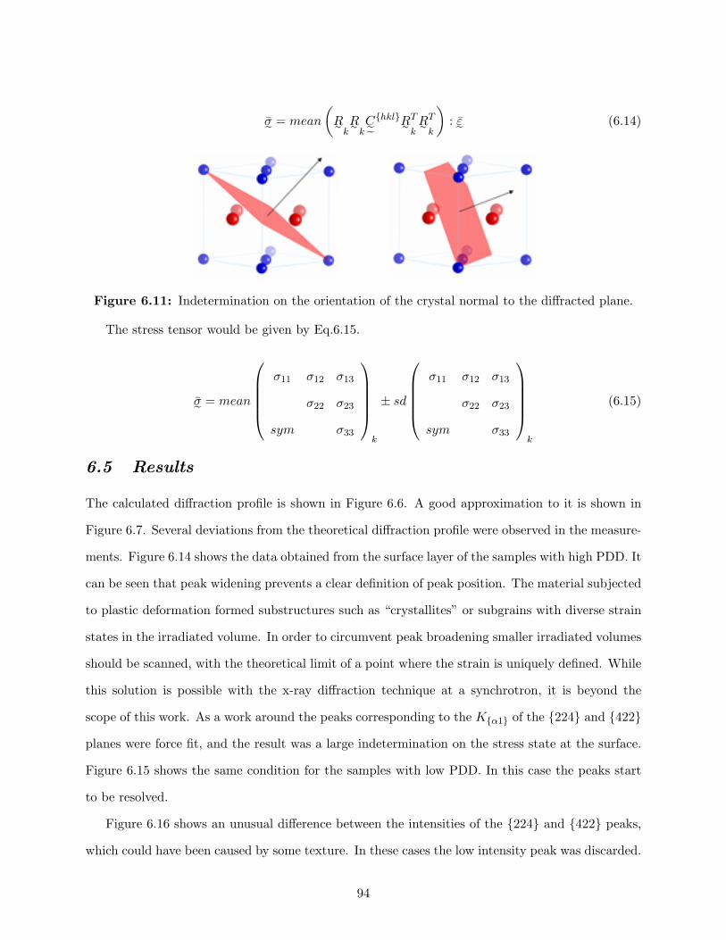
σ˜ = mean
(R∼
kR∼
kC˜hklR∼
T
kR∼
T
k
): ε˜ (6.14)
Figure 6.11: Indetermination on the orientation of the crystal normal to the diffracted plane.
The stress tensor would be given by Eq.6.15.
σ˜ = mean
σ11 σ12 σ13
σ22 σ23
sym σ33
k
± sd
σ11 σ12 σ13
σ22 σ23
sym σ33
k
(6.15)
6.5 Results
The calculated diffraction profile is shown in Figure 6.6. A good approximation to it is shown in
Figure 6.7. Several deviations from the theoretical diffraction profile were observed in the measure-
ments. Figure 6.14 shows the data obtained from the surface layer of the samples with high PDD. It
can be seen that peak widening prevents a clear definition of peak position. The material subjected
to plastic deformation formed substructures such as “crystallites” or subgrains with diverse strain
states in the irradiated volume. In order to circumvent peak broadening smaller irradiated volumes
should be scanned, with the theoretical limit of a point where the strain is uniquely defined. While
this solution is possible with the x-ray diffraction technique at a synchrotron, it is beyond the
scope of this work. As a work around the peaks corresponding to the Kα1 of the 224 and 422
planes were force fit, and the result was a large indetermination on the stress state at the surface.
Figure 6.15 shows the same condition for the samples with low PDD. In this case the peaks start
to be resolved.
Figure 6.16 shows an unusual difference between the intensities of the 224 and 422 peaks,
which could have been caused by some texture. In these cases the low intensity peak was discarded.
94
Figure 6.17 shows Kα2 peaks of almost same intensity as the Kα1. This could be caused by the
contribution of the 254 peak in the Ti3Al phase.
In the case of subsurface measurements, electropolishing was used to remove material, which
also affected the stress state on the measured layer. Also prolonged electropolishing caused the
increase of the material surface roughness. Figure 6.18 shows a contour plot of a 3D profilometry of
an electropolished sample. The peak to valley distance was approximately 60µm. The measurement
of a sample which such roughness would not indicate the stress state at the material bulk but rather
one at the asperities since the “shadow” produced by the asperities will prevent the radiation from
penetrating the surface below the asperities. Therefore, after electropolishing the sample was hand
polished using sand paper of grit 1200, 2400 and 4000 successively so that the surface roughness
was of a few microns. There is a modification of the residual stress due to this hand polishing
especially in the very superficial layers of the material considering that the energy of the x-rays
decays exponentially with the depth (i.e., the signal from the surface has more weight), however
this effect was not quantified in this work.
Plots for comparison of the fit of the theoretical strain to that measured are shown in Fig-
ures 6.12, and 6.13. The ordinates are the strain ε′33 while the abscissa shows the test number. The
segments joining adjacent points are only for representation purposes.
The summary of stress results is shown in Table 6.2. Figure 6.19 shows the longitudinal stress
for both high and low PDD. Figures 6.20, and 6.21 show the longitudinal and transversal stresses in
the case of high and low PDD respectively. Tables with an extended summary of results separated
by sample and family of planes can be found in Appendix B as well as the complete results of the
measurements and plots of goodness of fit comparisons.
6.6 Conclusions
Residual stresses were measured in 4 ground samples analyzing the effect of high and low PDD
value.
A generalized statistical data analysis was proposed based on the work of Winholtz and Cohen
(1988). This method considerably reduces the stress variance due to counting statistics and gra-
dients. In this method each strain measurement contributes to the determination of each strain
95
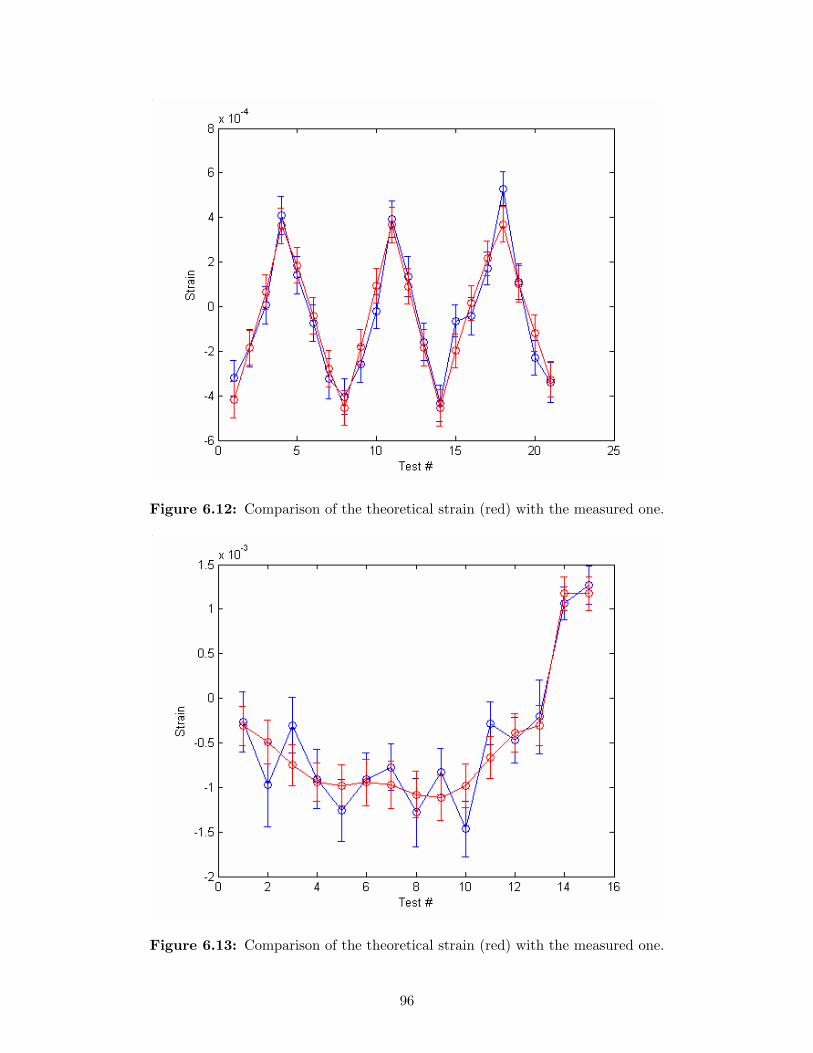
Figure 6.12: Comparison of the theoretical strain (red) with the measured one.
Figure 6.13: Comparison of the theoretical strain (red) with the measured one.
96
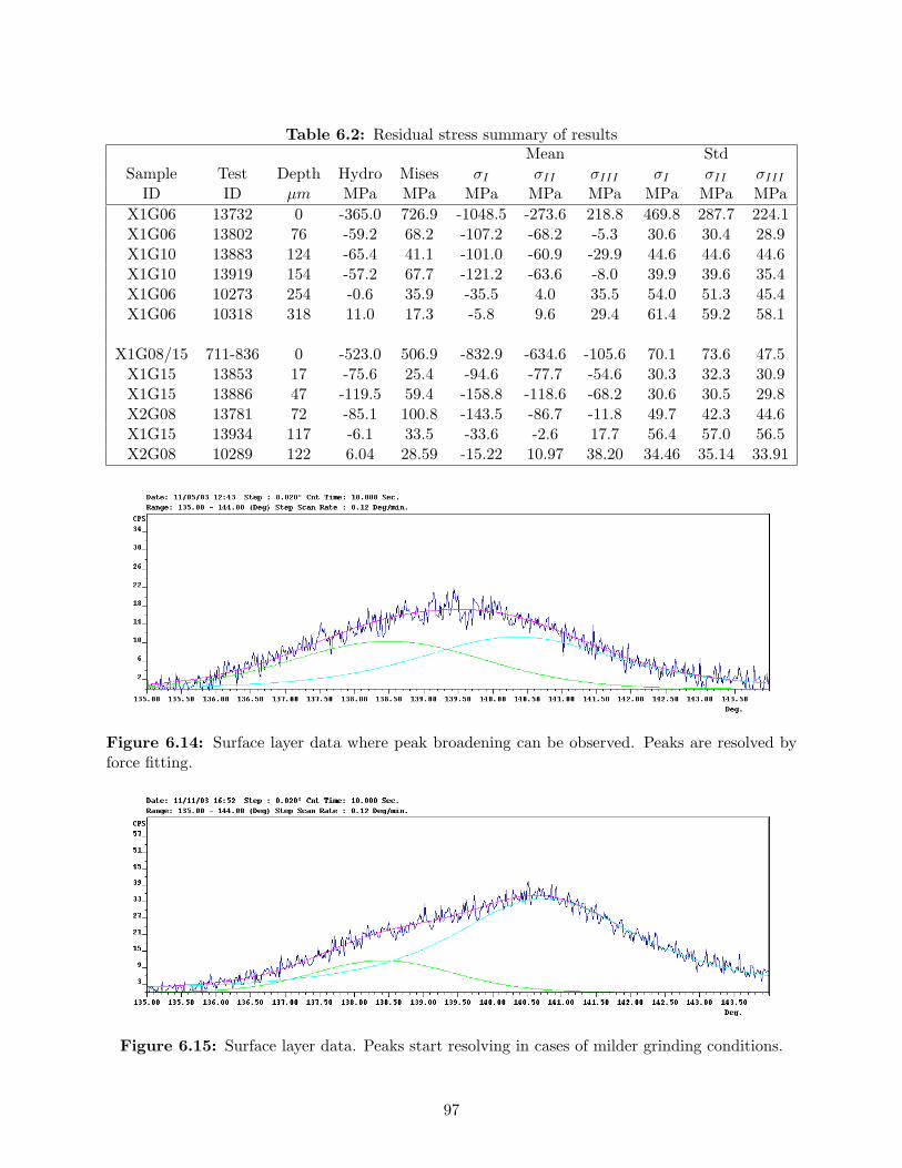
Table 6.2: Residual stress summary of resultsMean Std
Sample Test Depth Hydro Mises σI σII σIII σI σII σIII
ID ID µm MPa MPa MPa MPa MPa MPa MPa MPaX1G06 13732 0 -365.0 726.9 -1048.5 -273.6 218.8 469.8 287.7 224.1X1G06 13802 76 -59.2 68.2 -107.2 -68.2 -5.3 30.6 30.4 28.9X1G10 13883 124 -65.4 41.1 -101.0 -60.9 -29.9 44.6 44.6 44.6X1G10 13919 154 -57.2 67.7 -121.2 -63.6 -8.0 39.9 39.6 35.4X1G06 10273 254 -0.6 35.9 -35.5 4.0 35.5 54.0 51.3 45.4X1G06 10318 318 11.0 17.3 -5.8 9.6 29.4 61.4 59.2 58.1
X1G08/15 711-836 0 -523.0 506.9 -832.9 -634.6 -105.6 70.1 73.6 47.5X1G15 13853 17 -75.6 25.4 -94.6 -77.7 -54.6 30.3 32.3 30.9X1G15 13886 47 -119.5 59.4 -158.8 -118.6 -68.2 30.6 30.5 29.8X2G08 13781 72 -85.1 100.8 -143.5 -86.7 -11.8 49.7 42.3 44.6X1G15 13934 117 -6.1 33.5 -33.6 -2.6 17.7 56.4 57.0 56.5X2G08 10289 122 6.04 28.59 -15.22 10.97 38.20 34.46 35.14 33.91
Figure 6.14: Surface layer data where peak broadening can be observed. Peaks are resolved byforce fitting.
Figure 6.15: Surface layer data. Peaks start resolving in cases of milder grinding conditions.
97
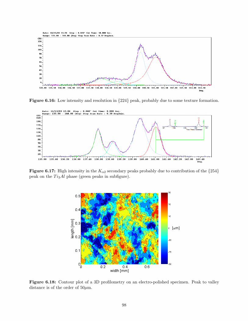
Figure 6.16: Low intensity and resolution in 224 peak, probably due to some texture formation.
Figure 6.17: High intensity in the Kα2 secondary peaks probably due to contribution of the 254peak on the Ti3Al phase (green peaks in subfigure).
Figure 6.18: Contour plot of a 3D profilometry on an electro-polished specimen. Peak to valleydistance is of the order of 50µm.
98
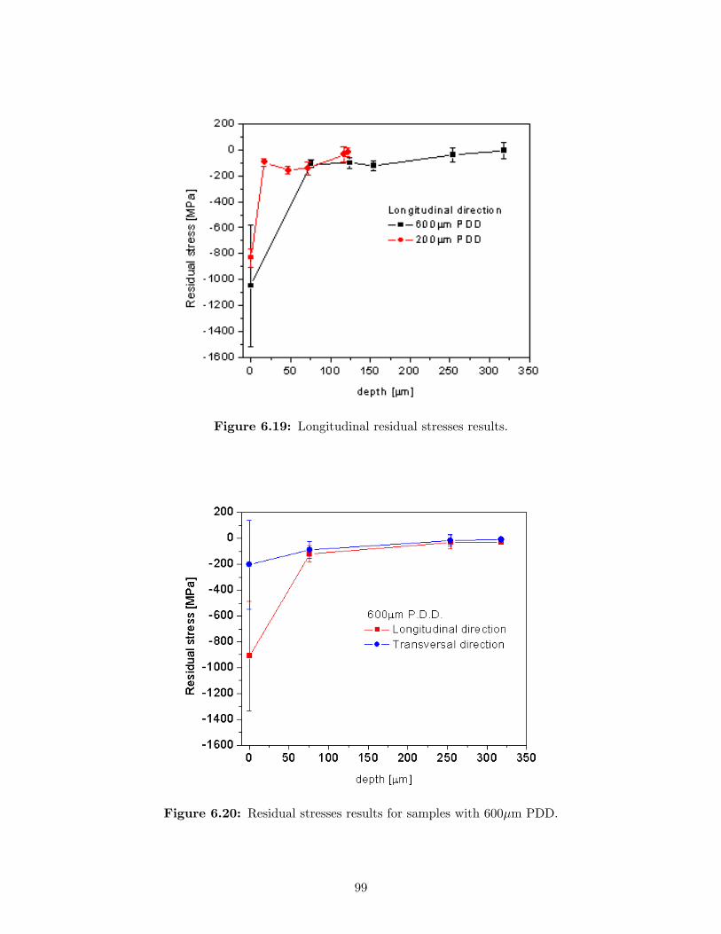
Figure 6.19: Longitudinal residual stresses results.
Figure 6.20: Residual stresses results for samples with 600µm PDD.
99
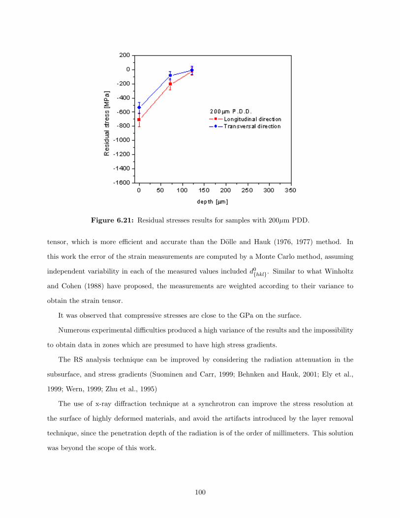
Figure 6.21: Residual stresses results for samples with 200µm PDD.
tensor, which is more efficient and accurate than the Dolle and Hauk (1976, 1977) method. In
this work the error of the strain measurements are computed by a Monte Carlo method, assuming
independent variability in each of the measured values included d0hkl. Similar to what Winholtz
and Cohen (1988) have proposed, the measurements are weighted according to their variance to
obtain the strain tensor.
It was observed that compressive stresses are close to the GPa on the surface.
Numerous experimental difficulties produced a high variance of the results and the impossibility
to obtain data in zones which are presumed to have high stress gradients.
The RS analysis technique can be improved by considering the radiation attenuation in the
subsurface, and stress gradients (Suominen and Carr, 1999; Behnken and Hauk, 2001; Ely et al.,
1999; Wern, 1999; Zhu et al., 1995)
The use of x-ray diffraction technique at a synchrotron can improve the stress resolution at
the surface of highly deformed materials, and avoid the artifacts introduced by the layer removal
technique, since the penetration depth of the radiation is of the order of millimeters. This solution
was beyond the scope of this work.
100
CHAPTER VII
ANALYTICAL MODELING
In this Chapter the indentation model proposed by Lawn and Wilshaw (1975); Aurora et al. (1979)
and used by Nelson (1997); Razavi (2000); and Stone (2003) to predict the depth of damage is
analyzed. The model proposed by Hecker (2002) to find the force per abrasive grit is used to
modify the indentation model and correlate it to PDD.
7.1 Indentation Model
Lawn and Wilshaw (1975) and Aurora et al. (1979) considered a brittle solid subjected to a normal
force F ′′N by a sharp pyramid indenter. A plastic zone was developed, and its extension (h0) given by
Eq. 7.1, where β is a dimensionless constant determined by plastic deformation zone geometry and
given by the ratio of h0 to half diagonal of the indentation, δ is a dimensionless constant determined
by the indenter geometry, and Hv is the Vickers hardness. The concept of this phenomenological
model is that the contact pressure generates a plastic zone which depends on the indenter geometry,
and the PDD, called here h0, independent of the indented size for a constant force. It assumes that
the contact pressure for inelastic deformation is independent of the indenter size and equal to the
material hardness, as assumed by the friction model proposed by Bowden and Tabor (1950).
h0 =(
β2
δπHv
)0.5
F ′′0.5N (7.1)
This model developed for a single indenter was modified by Nelson (1997) to include the normal force
in grinding using geometric and kinematic variables as proposed by Hahn and Lindsay (1982a,b)
and shown in Eq. 7.2, where Hg is the grinding hardness, b is the grinding width, Ew the workpiece
Young’s modulus, Vw the workpiece speed, and Vs the wheel’s tangential speed.
h0 =(
bβ2Ew
δπHg
)0.5(aVw
Vs
)0.5
(7.2)
Razavi (2000) used this model under force controlled conditions. Stone (2003) introduced the hard-
ness dependence on temperature into the model. The model proposed by Lawn and Wilshaw
101
(1975); and Aurora et al. (1979) considers an individual indenter under normal loads while in the
mentioned modifications the total grinding force was considered as the variable that controls PDD.
If the wheel total force FN and wheel/material area of contact (lcb) are considered for a typical
case, the mean contact pressure will be of the order of few MPa’s which could not explain the
existence of plastic deformation. Even though the original model as well as the modified model
are phenomenological in nature some physics is lost in the use of the total wheel normal force FN
instead of the individual grit normal force F ′′N . In this change in the scale of the model there is
no explicit account for the grit size of the abrasive, neither its concentration. It has been observed
in the results in Chapter 5 that wheels with different grit size produce different PDD under the
same FN . A direct address of the number of abrasives engaged in the process seems to be a more
sensible treatment to predict PDD. From the kinematic point of view these models only addressed
the dependence of PDD with F 0.5n . Differences in the number of active abrasives, bonding type,
and other grinding operation variables are considered by fitting the factor in front of FN for the
different conditions, limiting the results only to the case of study. Furthermore, some deviations
of the model with the data were observed by Nelson (1997) and correction factors were applied by
considering a force controlled setup (Razavi, 2000) and temperature effects (Stone, 2003) without
too much success.
This work proposes to explicitly address the influence of the number of abrasives in contact, find
the average force per abrasive, and used it as a predictor for PDD. The model developed by Hecker
(2002) was used.
7.2 Force per Abrasive Model
Several factors should be considered to model the force per grit. Grinding is a stochastic process,
with the wheel having a spatial distribution of abrasive grits. After dressing the wheel, some grits
will be exposed and a number will be active in the material removal process. In static measurements,
i.e. without any force or constraint acting on the wheel surface, it is possible to determine the
distribution of cutting edges versus distance to the wheel surface (z). With this information and
the grinding conditions it is possible to know how many abrasives will be engaged in the material
removal process in a few steps, but there are two effects that further modify this value. One is the
102
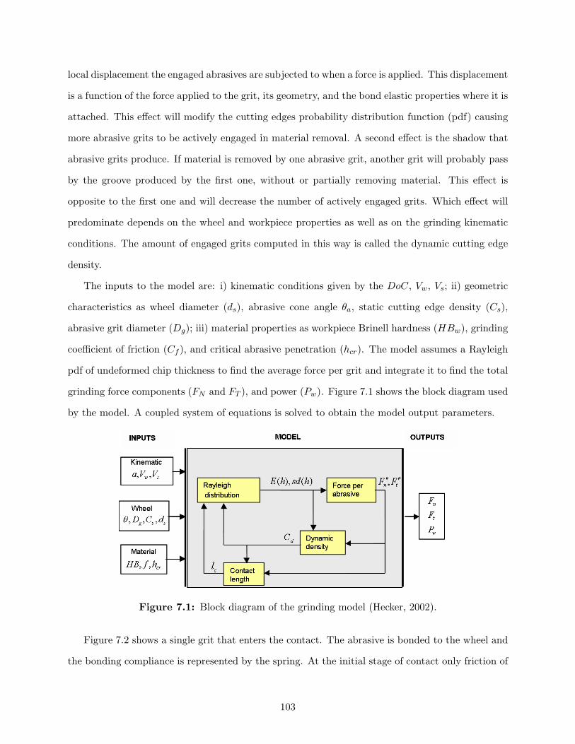
local displacement the engaged abrasives are subjected to when a force is applied. This displacement
is a function of the force applied to the grit, its geometry, and the bond elastic properties where it is
attached. This effect will modify the cutting edges probability distribution function (pdf) causing
more abrasive grits to be actively engaged in material removal. A second effect is the shadow that
abrasive grits produce. If material is removed by one abrasive grit, another grit will probably pass
by the groove produced by the first one, without or partially removing material. This effect is
opposite to the first one and will decrease the number of actively engaged grits. Which effect will
predominate depends on the wheel and workpiece properties as well as on the grinding kinematic
conditions. The amount of engaged grits computed in this way is called the dynamic cutting edge
density.
The inputs to the model are: i) kinematic conditions given by the DoC, Vw, Vs; ii) geometric
characteristics as wheel diameter (ds), abrasive cone angle θa, static cutting edge density (Cs),
abrasive grit diameter (Dg); iii) material properties as workpiece Brinell hardness (HBw), grinding
coefficient of friction (Cf ), and critical abrasive penetration (hcr). The model assumes a Rayleigh
pdf of undeformed chip thickness to find the average force per grit and integrate it to find the total
grinding force components (FN and FT ), and power (Pw). Figure 7.1 shows the block diagram used
by the model. A coupled system of equations is solved to obtain the model output parameters.
Figure 7.1: Block diagram of the grinding model (Hecker, 2002).
Figure 7.2 shows a single grit that enters the contact. The abrasive is bonded to the wheel and
the bonding compliance is represented by the spring. At the initial stage of contact only friction of
103
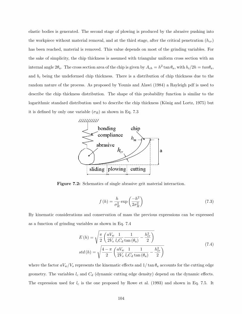
elastic bodies is generated. The second stage of plowing is produced by the abrasive pushing into
the workpiece without material removal, and at the third stage, after the critical penetration (hcr)
has been reached, material is removed. This value depends on most of the grinding variables. For
the sake of simplicity, the chip thickness is assumed with triangular uniform cross section with an
internal angle 2θa. The cross section area of the chip is given by Ach = h2 tan θa, with bc/2h = tanθa,
and bc being the undeformed chip thickness. There is a distribution of chip thickness due to the
random nature of the process. As proposed by Younis and Alawi (1984) a Rayleigh pdf is used to
describe the chip thickness distribution. The shape of this probability function is similar to the
logarithmic standard distribution used to describe the chip thickness (Konig and Lortz, 1975) but
it is defined by only one variable (σR) as shown in Eq. 7.3
Figure 7.2: Schematics of single abrasive grit material interaction.
f (h) =h
σ2R
exp(−h2
2σ2R
)(7.3)
By kinematic considerations and conservation of mass the previous expressions can be expressed
as a function of grinding variables as shown in Eq. 7.4
E (h) =
√π
2
(aVw
2Vs
1lcCd
1tan (θa)
− h2cr
2
)
std (h) =
√4− π
2
(aVw
2Vs
1lcCd
1tan (θa)
− h2cr
2
) (7.4)
where the factor aVw/Vs represents the kinematic effects and 1/ tan θa accounts for the cutting edge
geometry. The variables lc and Cd (dynamic cutting edge density) depend on the dynamic effects.
The expression used for lc is the one proposed by Rowe et al. (1993) and shown in Eq. 7.5. It
104
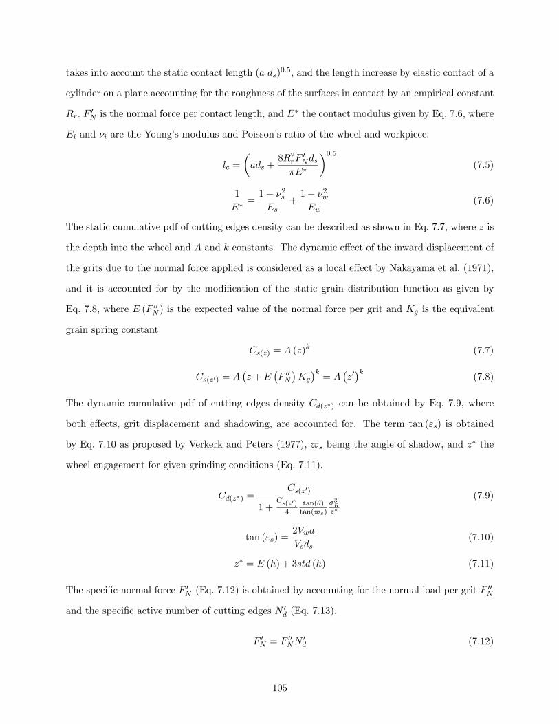
takes into account the static contact length (a ds)0.5, and the length increase by elastic contact of a
cylinder on a plane accounting for the roughness of the surfaces in contact by an empirical constant
Rr. F ′N is the normal force per contact length, and E∗ the contact modulus given by Eq. 7.6, where
Ei and νi are the Young’s modulus and Poisson’s ratio of the wheel and workpiece.
lc =(
ads +8R2
rF′Nds
πE∗
)0.5
(7.5)
1E∗ =
1− ν2s
Es+
1− ν2w
Ew(7.6)
The static cumulative pdf of cutting edges density can be described as shown in Eq. 7.7, where z is
the depth into the wheel and A and k constants. The dynamic effect of the inward displacement of
the grits due to the normal force applied is considered as a local effect by Nakayama et al. (1971),
and it is accounted for by the modification of the static grain distribution function as given by
Eq. 7.8, where E (F ′′N ) is the expected value of the normal force per grit and Kg is the equivalent
grain spring constant
Cs(z) = A (z)k (7.7)
Cs(z′) = A(z + E
(F ′′
N
)Kg
)k = A(z′)k (7.8)
The dynamic cumulative pdf of cutting edges density Cd(z∗) can be obtained by Eq. 7.9, where
both effects, grit displacement and shadowing, are accounted for. The term tan (εs) is obtained
by Eq. 7.10 as proposed by Verkerk and Peters (1977), $s being the angle of shadow, and z∗ the
wheel engagement for given grinding conditions (Eq. 7.11).
Cd(z∗) =Cs(z′)
1 +Cs(z′)
4tan(θ)
tan($s)
σ3R
z∗
(7.9)
tan (εs) =2Vwa
Vsds(7.10)
z∗ = E (h) + 3std (h) (7.11)
The specific normal force F ′N (Eq. 7.12) is obtained by accounting for the normal load per grit F ′′
N
and the specific active number of cutting edges N ′d (Eq. 7.13).
F ′N = F ′′
NN ′d (7.12)
105
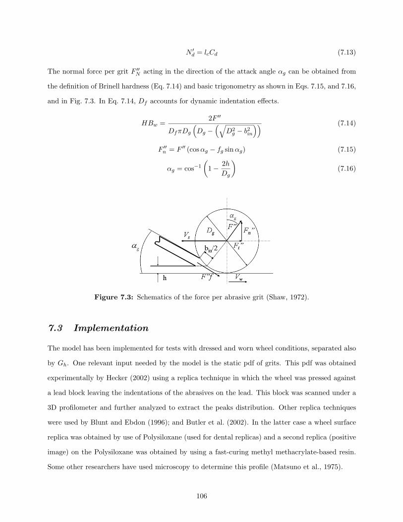
N ′d = lcCd (7.13)
The normal force per grit F ′′N acting in the direction of the attack angle αg can be obtained from
the definition of Brinell hardness (Eq. 7.14) and basic trigonometry as shown in Eqs. 7.15, and 7.16,
and in Fig. 7.3. In Eq. 7.14, Df accounts for dynamic indentation effects.
HBw =2F ′′
DfπDg
(Dg −
(√D2
g − b2in
)) (7.14)
F ′′n = F ′′ (cos αg − fg sinαg) (7.15)
αg = cos−1
(1− 2h
Dg
)(7.16)
Figure 7.3: Schematics of the force per abrasive grit (Shaw, 1972).
7.3 Implementation
The model has been implemented for tests with dressed and worn wheel conditions, separated also
by Gh. One relevant input needed by the model is the static pdf of grits. This pdf was obtained
experimentally by Hecker (2002) using a replica technique in which the wheel was pressed against
a lead block leaving the indentations of the abrasives on the lead. This block was scanned under a
3D profilometer and further analyzed to extract the peaks distribution. Other replica techniques
were used by Blunt and Ebdon (1996); and Butler et al. (2002). In the latter case a wheel surface
replica was obtained by use of Polysiloxane (used for dental replicas) and a second replica (positive
image) on the Polysiloxane was obtained by using a fast-curing methyl methacrylate-based resin.
Some other researchers have used microscopy to determine this profile (Matsuno et al., 1975).
106
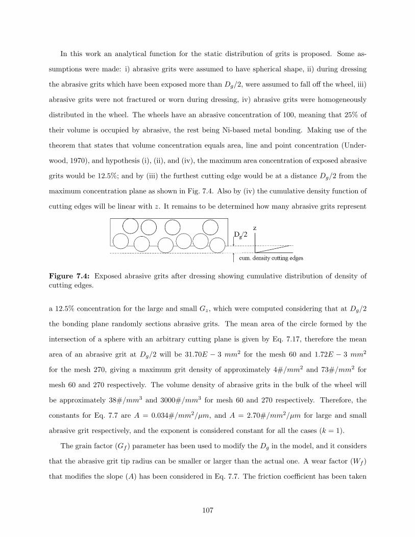
In this work an analytical function for the static distribution of grits is proposed. Some as-
sumptions were made: i) abrasive grits were assumed to have spherical shape, ii) during dressing
the abrasive grits which have been exposed more than Dg/2, were assumed to fall off the wheel, iii)
abrasive grits were not fractured or worn during dressing, iv) abrasive grits were homogeneously
distributed in the wheel. The wheels have an abrasive concentration of 100, meaning that 25% of
their volume is occupied by abrasive, the rest being Ni-based metal bonding. Making use of the
theorem that states that volume concentration equals area, line and point concentration (Under-
wood, 1970), and hypothesis (i), (ii), and (iv), the maximum area concentration of exposed abrasive
grits would be 12.5%; and by (iii) the furthest cutting edge would be at a distance Dg/2 from the
maximum concentration plane as shown in Fig. 7.4. Also by (iv) the cumulative density function of
cutting edges will be linear with z. It remains to be determined how many abrasive grits represent
Figure 7.4: Exposed abrasive grits after dressing showing cumulative distribution of density ofcutting edges.
a 12.5% concentration for the large and small Gz, which were computed considering that at Dg/2
the bonding plane randomly sections abrasive grits. The mean area of the circle formed by the
intersection of a sphere with an arbitrary cutting plane is given by Eq. 7.17, therefore the mean
area of an abrasive grit at Dg/2 will be 31.70E − 3 mm2 for the mesh 60 and 1.72E − 3 mm2
for the mesh 270, giving a maximum grit density of approximately 4#/mm2 and 73#/mm2 for
mesh 60 and 270 respectively. The volume density of abrasive grits in the bulk of the wheel will
be approximately 38#/mm3 and 3000#/mm3 for mesh 60 and 270 respectively. Therefore, the
constants for Eq. 7.7 are A = 0.034#/mm2/µm, and A = 2.70#/mm2/µm for large and small
abrasive grit respectively, and the exponent is considered constant for all the cases (k = 1).
The grain factor (Gf ) parameter has been used to modify the Dg in the model, and it considers
that the abrasive grit tip radius can be smaller or larger than the actual one. A wear factor (Wf )
that modifies the slope (A) has been considered in Eq. 7.7. The friction coefficient has been taken
107
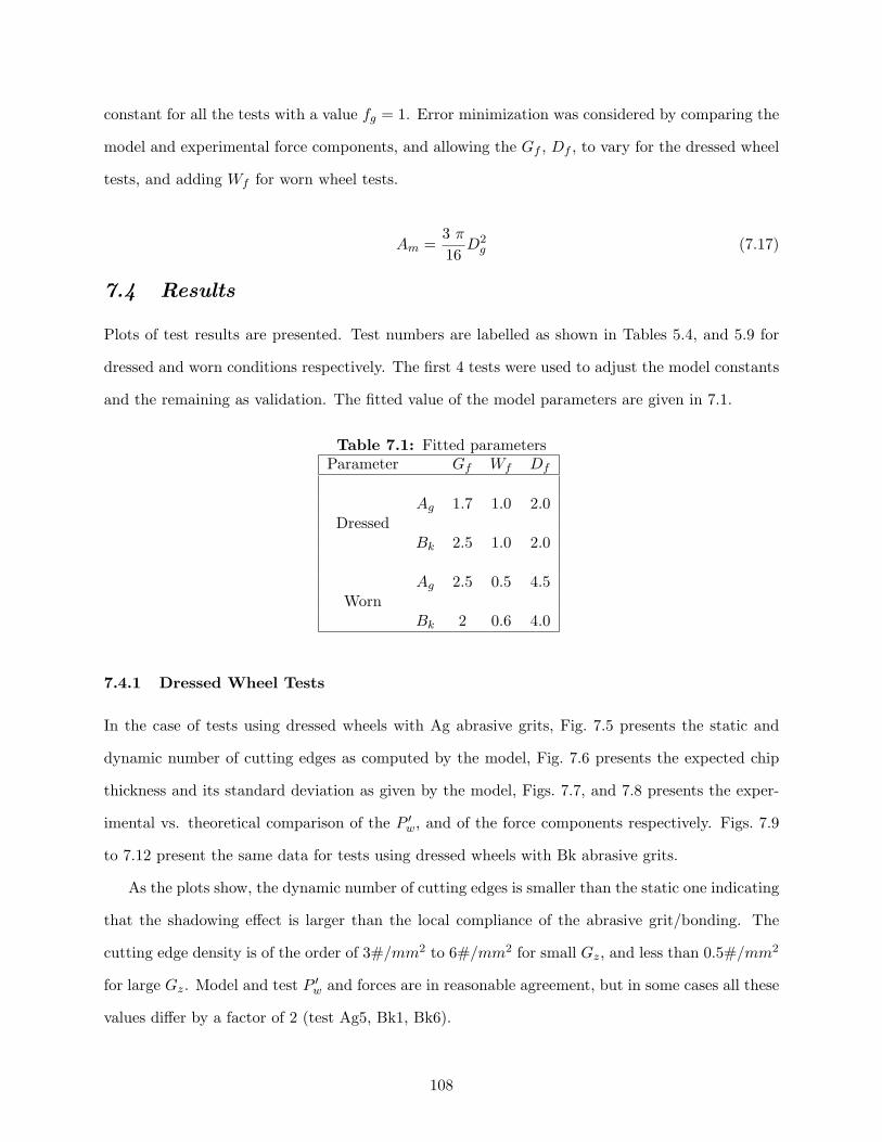
constant for all the tests with a value fg = 1. Error minimization was considered by comparing the
model and experimental force components, and allowing the Gf , Df , to vary for the dressed wheel
tests, and adding Wf for worn wheel tests.
Am =3 π
16D2
g (7.17)
7.4 Results
Plots of test results are presented. Test numbers are labelled as shown in Tables 5.4, and 5.9 for
dressed and worn conditions respectively. The first 4 tests were used to adjust the model constants
and the remaining as validation. The fitted value of the model parameters are given in 7.1.
Table 7.1: Fitted parametersParameter Gf Wf Df
Ag 1.7 1.0 2.0Dressed
Bk 2.5 1.0 2.0
Ag 2.5 0.5 4.5Worn
Bk 2 0.6 4.0
7.4.1 Dressed Wheel Tests
In the case of tests using dressed wheels with Ag abrasive grits, Fig. 7.5 presents the static and
dynamic number of cutting edges as computed by the model, Fig. 7.6 presents the expected chip
thickness and its standard deviation as given by the model, Figs. 7.7, and 7.8 presents the exper-
imental vs. theoretical comparison of the P ′w, and of the force components respectively. Figs. 7.9
to 7.12 present the same data for tests using dressed wheels with Bk abrasive grits.
As the plots show, the dynamic number of cutting edges is smaller than the static one indicating
that the shadowing effect is larger than the local compliance of the abrasive grit/bonding. The
cutting edge density is of the order of 3#/mm2 to 6#/mm2 for small Gz, and less than 0.5#/mm2
for large Gz. Model and test P ′w and forces are in reasonable agreement, but in some cases all these
values differ by a factor of 2 (test Ag5, Bk1, Bk6).
108
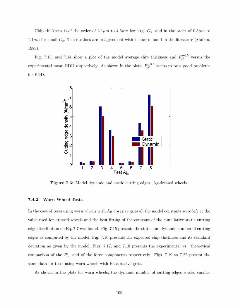
Chip thickness is of the order of 2.1µm to 4.5µm for large Gz, and in the order of 0.5µm to
1.1µm for small Gz. These values are in agreement with the ones found in the literature (Malkin,
1989).
Fig. 7.13, and 7.14 show a plot of the model average chip thickness and F ′′N
0.5 versus the
experimental mean PDD respectively. As shown in the plots, F ′′N
0.5 seems to be a good predictor
for PDD.
Figure 7.5: Model dynamic and static cutting edges. Ag-dressed wheels.
7.4.2 Worn Wheel Tests
In the case of tests using worn wheels with Ag abrasive grits all the model constants were left at the
value used for dressed wheels and the best fitting of the constant of the cumulative static cutting
edge distribution on Eq. 7.7 was found. Fig. 7.15 presents the static and dynamic number of cutting
edges as computed by the model, Fig. 7.16 presents the expected chip thickness and its standard
deviation as given by the model, Figs. 7.17, and 7.18 presents the experimental vs. theoretical
comparison of the P ′w, and of the force components respectively. Figs. 7.19 to 7.22 present the
same data for tests using worn wheels with Bk abrasive grits.
As shown in the plots for worn wheels, the dynamic number of cutting edges is also smaller
109
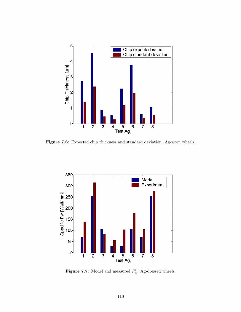
Figure 7.6: Expected chip thickness and standard deviation. Ag-worn wheels.
Figure 7.7: Model and measured P ′w. Ag-dressed wheels.
110
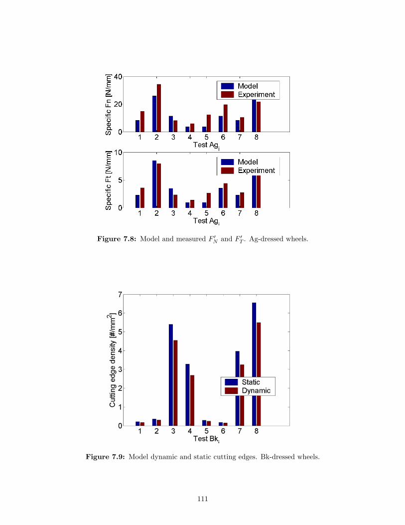
Figure 7.8: Model and measured F ′N and F ′
T . Ag-dressed wheels.
Figure 7.9: Model dynamic and static cutting edges. Bk-dressed wheels.
111
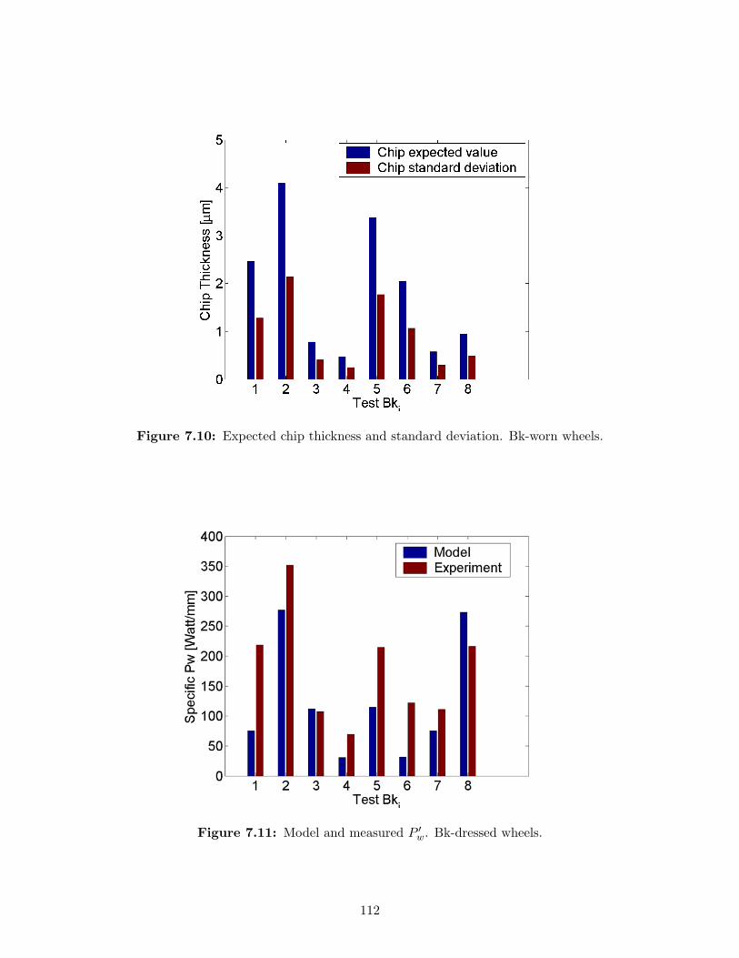
Figure 7.10: Expected chip thickness and standard deviation. Bk-worn wheels.
Figure 7.11: Model and measured P ′w. Bk-dressed wheels.
112
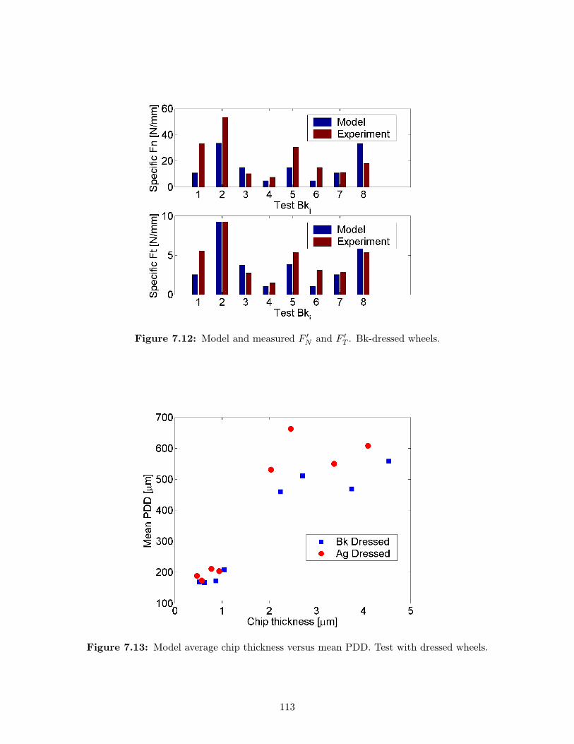
Figure 7.12: Model and measured F ′N and F ′
T . Bk-dressed wheels.
Figure 7.13: Model average chip thickness versus mean PDD. Test with dressed wheels.
113
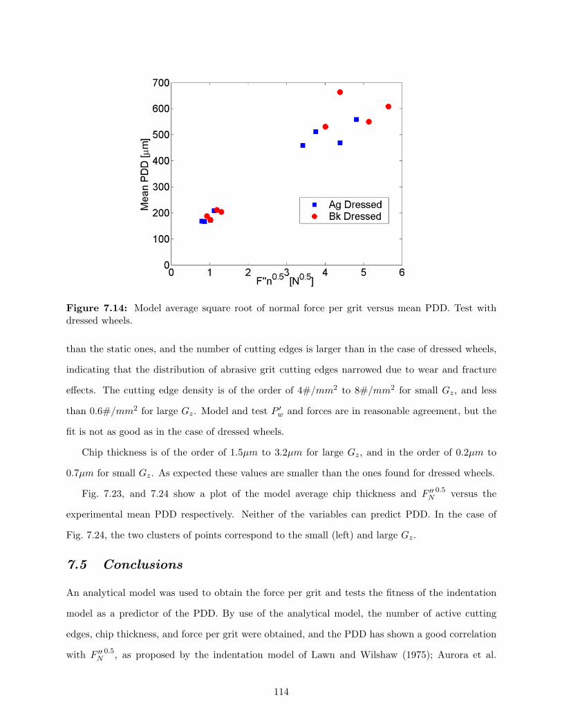
Figure 7.14: Model average square root of normal force per grit versus mean PDD. Test withdressed wheels.
than the static ones, and the number of cutting edges is larger than in the case of dressed wheels,
indicating that the distribution of abrasive grit cutting edges narrowed due to wear and fracture
effects. The cutting edge density is of the order of 4#/mm2 to 8#/mm2 for small Gz, and less
than 0.6#/mm2 for large Gz. Model and test P ′w and forces are in reasonable agreement, but the
fit is not as good as in the case of dressed wheels.
Chip thickness is of the order of 1.5µm to 3.2µm for large Gz, and in the order of 0.2µm to
0.7µm for small Gz. As expected these values are smaller than the ones found for dressed wheels.
Fig. 7.23, and 7.24 show a plot of the model average chip thickness and F ′′N
0.5 versus the
experimental mean PDD respectively. Neither of the variables can predict PDD. In the case of
Fig. 7.24, the two clusters of points correspond to the small (left) and large Gz.
7.5 Conclusions
An analytical model was used to obtain the force per grit and tests the fitness of the indentation
model as a predictor of the PDD. By use of the analytical model, the number of active cutting
edges, chip thickness, and force per grit were obtained, and the PDD has shown a good correlation
with F ′′N
0.5, as proposed by the indentation model of Lawn and Wilshaw (1975); Aurora et al.
114
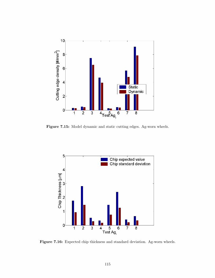
Figure 7.15: Model dynamic and static cutting edges. Ag-worn wheels.
Figure 7.16: Expected chip thickness and standard deviation. Ag-worn wheels.
115
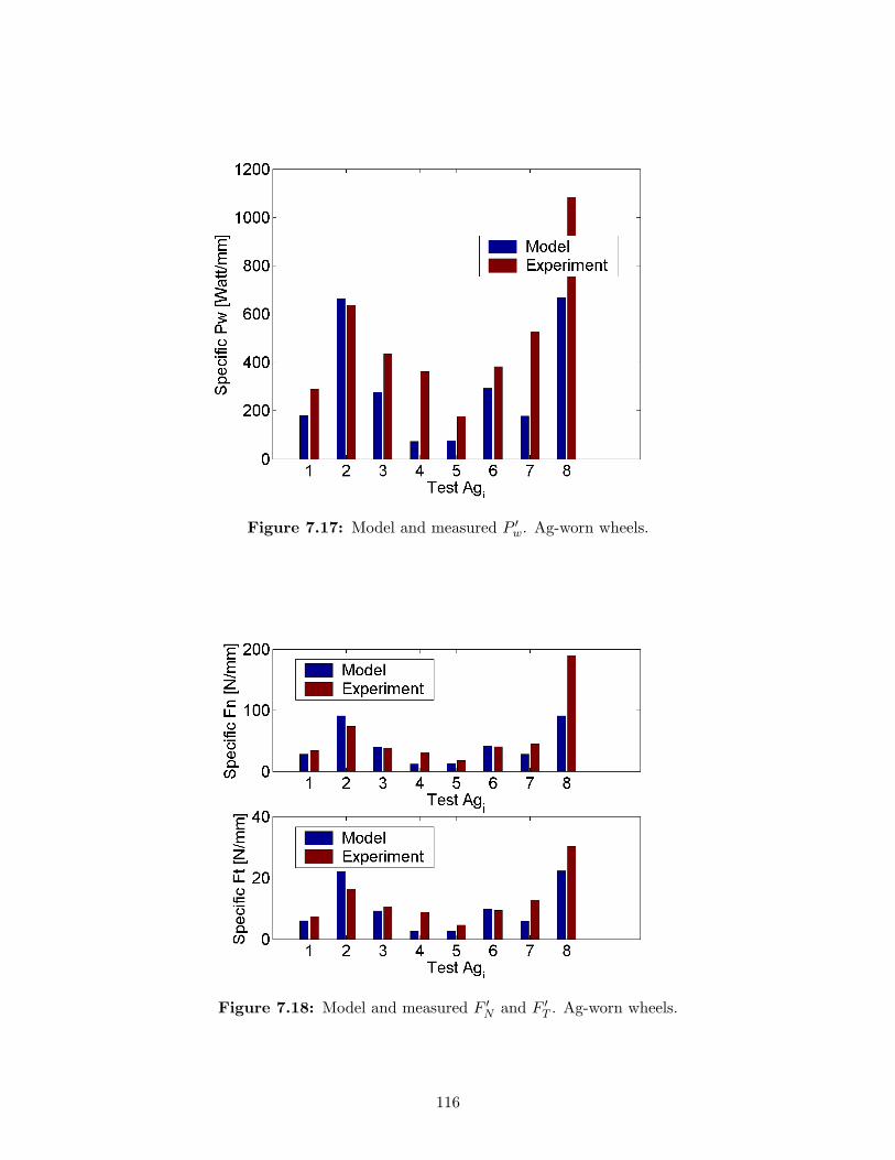
Figure 7.17: Model and measured P ′w. Ag-worn wheels.
Figure 7.18: Model and measured F ′N and F ′
T . Ag-worn wheels.
116
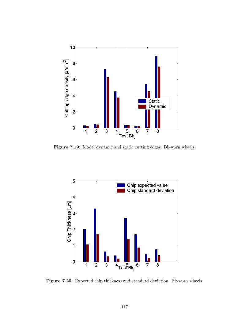
Figure 7.19: Model dynamic and static cutting edges. Bk-worn wheels.
Figure 7.20: Expected chip thickness and standard deviation. Bk-worn wheels.
117
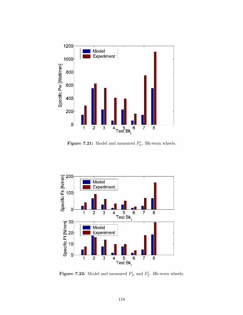
Figure 7.21: Model and measured P ′w. Bk-worn wheels.
Figure 7.22: Model and measured F ′N and F ′
T . Bk-worn wheels.
118
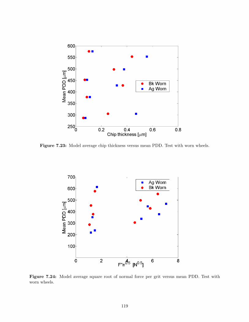
Figure 7.23: Model average chip thickness versus mean PDD. Test with worn wheels.
Figure 7.24: Model average square root of normal force per grit versus mean PDD. Test withworn wheels.
119
(1979). This suggests that the indentation model is still valid for grinding if the force per grit is
used instead of the total grinding force.
The model captures the difference in the number of cutting edges and chip thickness for the
different Gz.
The results show that the model captures the effect of wear by fitting the values of grinding
total force in an acceptable manner. Nevertheless, the model attributes the increase of the normal
force in the case of worn wheels to dynamic effects. The fitted dynamic factor Df for the worn
wheel was twice from the one obtained for dressed wheels. The number of cutting edges and the
force per grit remains approximately in the same range for the two wear conditions, which is a
dubious result.
For the dressed conditions, the analytical model predicts a cutting edge density of the order of
3#/mm2 to 6#/mm2 for small Gz, and less than 0.5#/mm2 for large Gz. Model and test P ′w and
forces are in reasonable agreement, but in some cases all these values differ by a factor of 2.
Chip thickness is of the order of 2.1µm to 4.5µm for large Gz, and in the order of 0.5µm to
1.1µm for small Gz. These values are in agreement with the ones found in the literature.
The analytical model predicts for the worn conditions that‘ the cutting edge density is of the
order of 4#/mm2 to 8#/mm2 for small Gz, and less than 0.6#/mm2 for large Gz. The chip
thickness is of the order of 1.5µm to 3.2µm for large Gz, and in the order of 0.2µm to 0.7µm for
small Gz. As expected these values are smaller than the ones found for dressed wheels.
The resulting fitted factors of the analytical model might indicate that the model works well
for dressed conditions by capturing expected trends, but it does not give good predictions for
worn conditions. This difference might be due to variables not accounted for such as temperature,
possible contact of bond material with the workpiece for small Gz, or a probability density function
of cutting edges density different from the one assumed in this work.
120
CHAPTER VIII
NUMERICAL MODELING
An isotropic rate dependent elastic-plastic model, and an anisotropic elastic-viscoplastic crystal
plasticity model were used in 2D and 3D geometric models under different BC’s to analyze: i)
behavior of the PDD vs. F ′′n plots for different indenter sizes; ii) validity of Eq. 7.1 to predict
PDD under scratching conditions; iii) PDD relation for PE vs. PS and its implications to the PDD
measuring technique described in Chapter 4; iv) effect of lamellae orientation and lamellae boundary
on PDD; v) verification of the force per grit obtained by the model presented in Chapter 7. The
models were implemented in ABAQUS v6.3. Due to the nonlinearity of the material response and
large sliding conditions, the explicit integration scheme was used. Adaptive meshing was used to
improve the element aspect ratio under large deformations. To increase stability, bulk viscosity was
activated with a linear parameter of 0.12 and a quadratic one of 2.4 (Abaqus, 2001). The indenter
was modeled as an analytical surface (rigid body). The friction coefficient was set at 0.1 for all
tests.
8.1 Isotropic Elastic-plastic Model Simulations
The material isotropic elastic properties used were E = 178E3, and ν = 0.23. The isotropic plastic
properties were modeled by entering the piecewise curves of Fig. 3.10. Von Mises plasticity criterion
was used with isotropic hardening.
8.1.1 Model Validation
The model was validated by the simulation of indentation tests and their comparison with experi-
mental results. A 2D model of a 3.5mm radius by 3mm high cylinder was meshed using CAX4R
4-node bilinear, reduced integration with hourglass control, axisymmetric solid elements. The
model had 10002 elements with a total of 20404 DOF (degrees of freedom). The element resolution
at the contact zone was of 3.5µm. The indenter geometry was sphero-conic with 200µm tip radius
and 60 cone semiangle. Figures 8.1, and 8.2 show the complete, and contact zone close-up of the
121
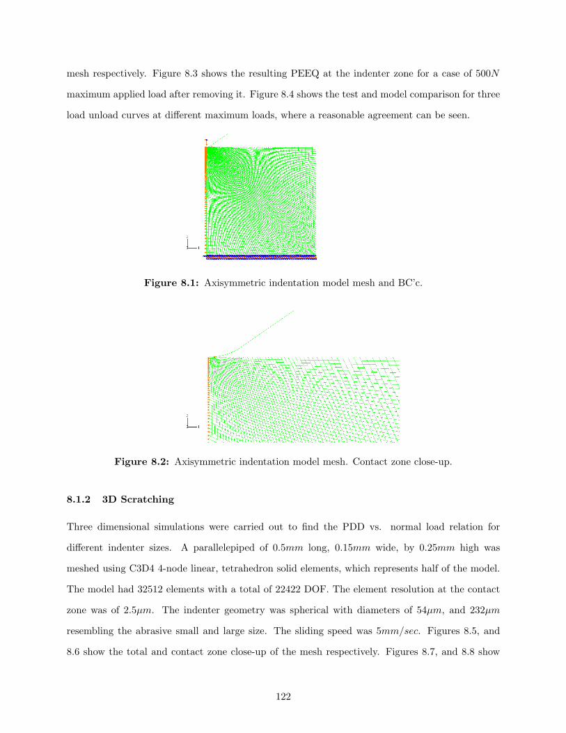
mesh respectively. Figure 8.3 shows the resulting PEEQ at the indenter zone for a case of 500N
maximum applied load after removing it. Figure 8.4 shows the test and model comparison for three
load unload curves at different maximum loads, where a reasonable agreement can be seen.
Figure 8.1: Axisymmetric indentation model mesh and BC’c.
Figure 8.2: Axisymmetric indentation model mesh. Contact zone close-up.
8.1.2 3D Scratching
Three dimensional simulations were carried out to find the PDD vs. normal load relation for
different indenter sizes. A parallelepiped of 0.5mm long, 0.15mm wide, by 0.25mm high was
meshed using C3D4 4-node linear, tetrahedron solid elements, which represents half of the model.
The model had 32512 elements with a total of 22422 DOF. The element resolution at the contact
zone was of 2.5µm. The indenter geometry was spherical with diameters of 54µm, and 232µm
resembling the abrasive small and large size. The sliding speed was 5mm/sec. Figures 8.5, and
8.6 show the total and contact zone close-up of the mesh respectively. Figures 8.7, and 8.8 show
122
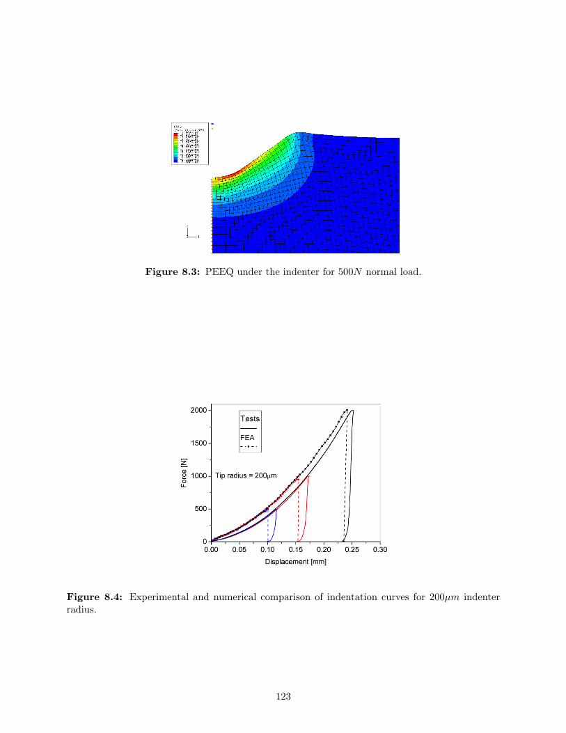
Figure 8.3: PEEQ under the indenter for 500N normal load.
Figure 8.4: Experimental and numerical comparison of indentation curves for 200µm indenterradius.
123
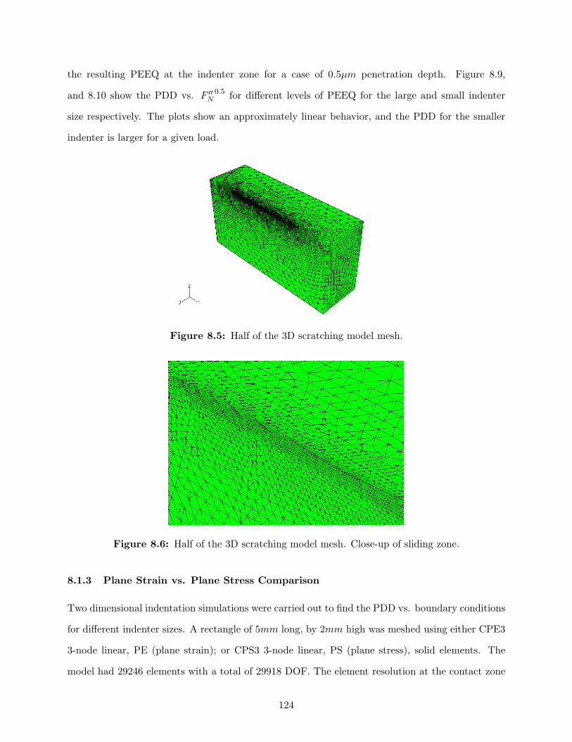
the resulting PEEQ at the indenter zone for a case of 0.5µm penetration depth. Figure 8.9,
and 8.10 show the PDD vs. F ′′N
0.5 for different levels of PEEQ for the large and small indenter
size respectively. The plots show an approximately linear behavior, and the PDD for the smaller
indenter is larger for a given load.
Figure 8.5: Half of the 3D scratching model mesh.
Figure 8.6: Half of the 3D scratching model mesh. Close-up of sliding zone.
8.1.3 Plane Strain vs. Plane Stress Comparison
Two dimensional indentation simulations were carried out to find the PDD vs. boundary conditions
for different indenter sizes. A rectangle of 5mm long, by 2mm high was meshed using either CPE3
3-node linear, PE (plane strain); or CPS3 3-node linear, PS (plane stress), solid elements. The
model had 29246 elements with a total of 29918 DOF. The element resolution at the contact zone
124
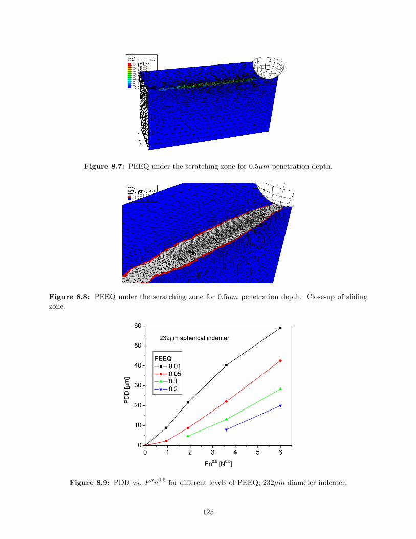
Figure 8.7: PEEQ under the scratching zone for 0.5µm penetration depth.
Figure 8.8: PEEQ under the scratching zone for 0.5µm penetration depth. Close-up of slidingzone.
Figure 8.9: PDD vs. F ′′n0.5 for different levels of PEEQ; 232µm diameter indenter.
125
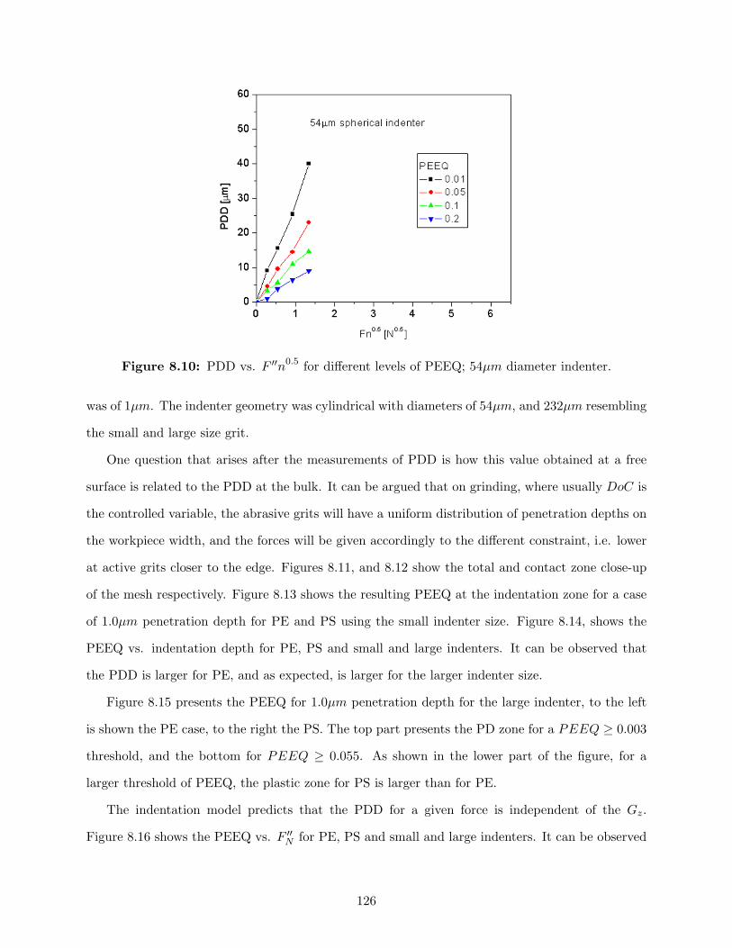
Figure 8.10: PDD vs. F ′′n0.5 for different levels of PEEQ; 54µm diameter indenter.
was of 1µm. The indenter geometry was cylindrical with diameters of 54µm, and 232µm resembling
the small and large size grit.
One question that arises after the measurements of PDD is how this value obtained at a free
surface is related to the PDD at the bulk. It can be argued that on grinding, where usually DoC is
the controlled variable, the abrasive grits will have a uniform distribution of penetration depths on
the workpiece width, and the forces will be given accordingly to the different constraint, i.e. lower
at active grits closer to the edge. Figures 8.11, and 8.12 show the total and contact zone close-up
of the mesh respectively. Figure 8.13 shows the resulting PEEQ at the indentation zone for a case
of 1.0µm penetration depth for PE and PS using the small indenter size. Figure 8.14, shows the
PEEQ vs. indentation depth for PE, PS and small and large indenters. It can be observed that
the PDD is larger for PE, and as expected, is larger for the larger indenter size.
Figure 8.15 presents the PEEQ for 1.0µm penetration depth for the large indenter, to the left
is shown the PE case, to the right the PS. The top part presents the PD zone for a PEEQ ≥ 0.003
threshold, and the bottom for PEEQ ≥ 0.055. As shown in the lower part of the figure, for a
larger threshold of PEEQ, the plastic zone for PS is larger than for PE.
The indentation model predicts that the PDD for a given force is independent of the Gz.
Figure 8.16 shows the PEEQ vs. F ′′N for PE, PS and small and large indenters. It can be observed
126
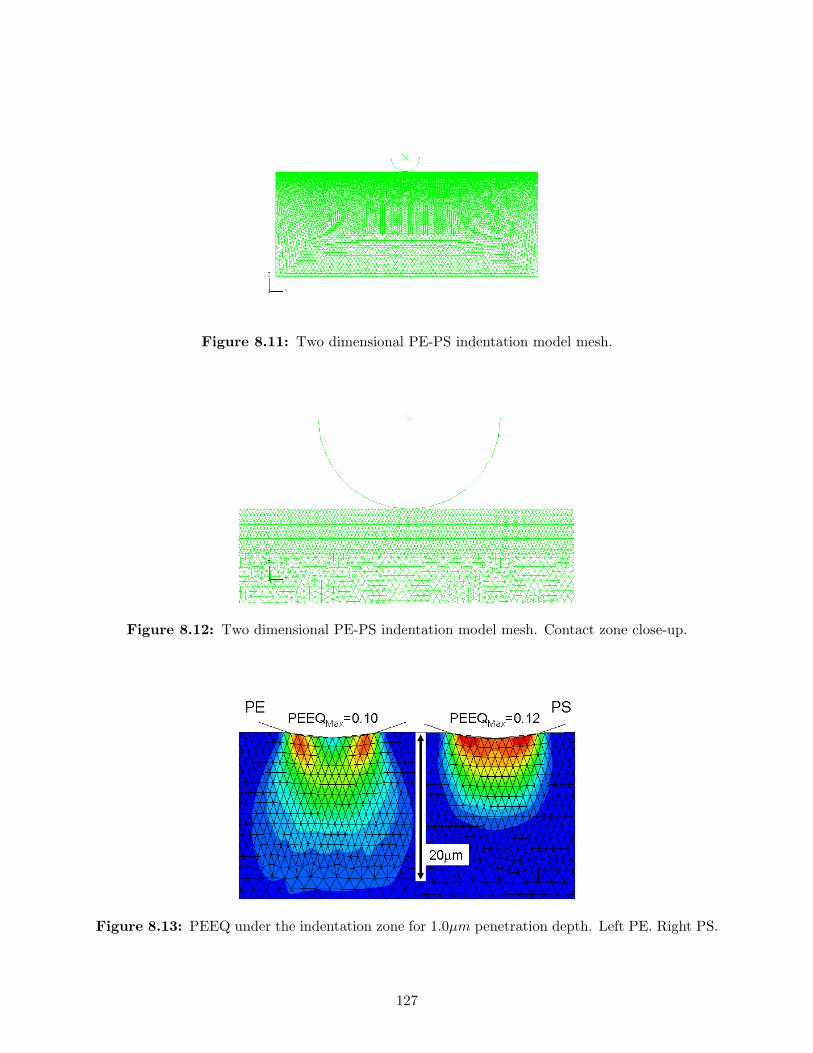
Figure 8.11: Two dimensional PE-PS indentation model mesh.
Figure 8.12: Two dimensional PE-PS indentation model mesh. Contact zone close-up.
Figure 8.13: PEEQ under the indentation zone for 1.0µm penetration depth. Left PE. Right PS.
127
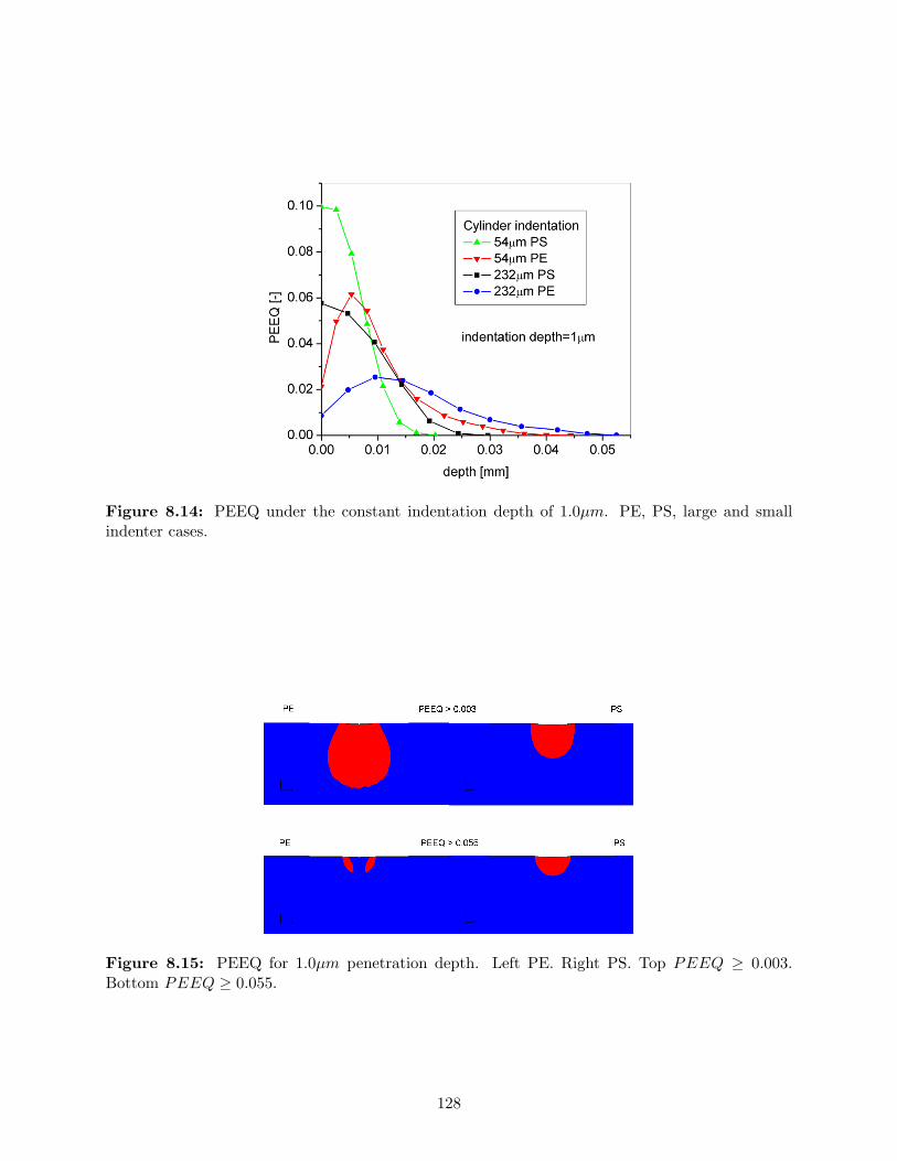
Figure 8.14: PEEQ under the constant indentation depth of 1.0µm. PE, PS, large and smallindenter cases.
Figure 8.15: PEEQ for 1.0µm penetration depth. Left PE. Right PS. Top PEEQ ≥ 0.003.Bottom PEEQ ≥ 0.055.
128
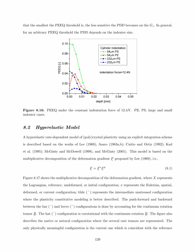
that the smallest the PEEQ threshold is, the less sensitive the PDD becomes on the Gz. In general,
for an arbitrary PEEQ threshold the PDD depends on the indenter size.
Figure 8.16: PEEQ under the constant indentation force of 12.4N . PE, PS, large and smallindenter cases.
8.2 Hyperelastic Model
A hyperelastic rate-dependent model of (poly)crystal plasticity using an explicit integration scheme
is described based on the works of Lee (1969); Asaro (1983a,b); Cuitio and Ortiz (1992); Kad
et al. (1995); McGinty and McDowell (1999), and McGinty (2001). This model is based on the
multiplicative decomposition of the deformation gradient F∼ proposed by Lee (1969), i.e.,
F∼ = F∼eF∼
p (8.1)
Figure 8.17 shows the multiplicative decomposition of the deformation gradient, where X represents
the Lagrangian, reference, undeformed, or initial configuration; x represents the Eulerian, spatial,
deformed, or current configuration; tilde (˜) represents the intermediate unstressed configuration
where the plasticity constitutive modeling is better described. The push-forward and backward
between the bar (¯) and breve (˘) configurations is done by accounting for the continuum rotation
tensor R∼ . The hat (ˆ) configuration is corotational with the continuum rotation R∼ . The figure also
describes the native or natural configuration where the several rate tensors are represented. The
only physically meaningful configuration is the current one which is coincident with the reference
129
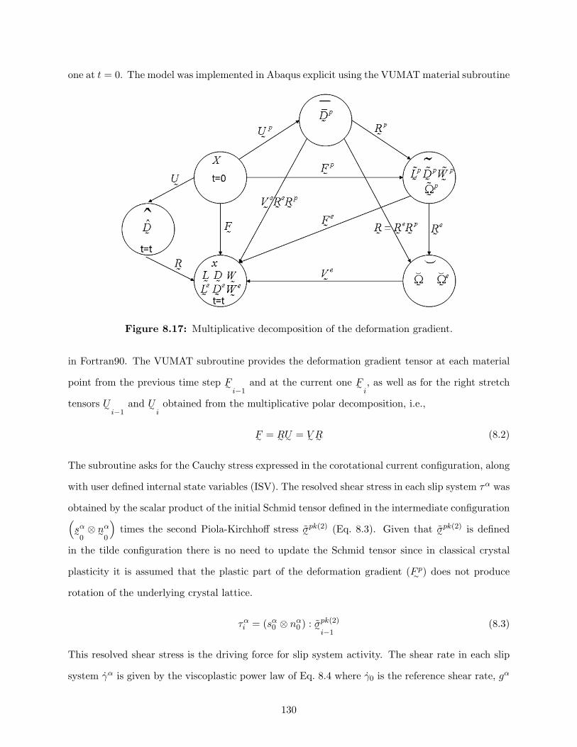
one at t = 0. The model was implemented in Abaqus explicit using the VUMAT material subroutine
Figure 8.17: Multiplicative decomposition of the deformation gradient.
in Fortran90. The VUMAT subroutine provides the deformation gradient tensor at each material
point from the previous time step F∼i−1
and at the current one F∼i, as well as for the right stretch
tensors U∼i−1
and U∼iobtained from the multiplicative polar decomposition, i.e.,
F∼ = R∼U∼ = V∼ R∼ (8.2)
The subroutine asks for the Cauchy stress expressed in the corotational current configuration, along
with user defined internal state variables (ISV). The resolved shear stress in each slip system τα was
obtained by the scalar product of the initial Schmid tensor defined in the intermediate configuration(s∼
α
0⊗ n∼
α
0
)times the second Piola-Kirchhoff stress σ∼
pk(2) (Eq. 8.3). Given that σ∼pk(2) is defined
in the tilde configuration there is no need to update the Schmid tensor since in classical crystal
plasticity it is assumed that the plastic part of the deformation gradient (F p∼ ) does not produce
rotation of the underlying crystal lattice.
ταi = (sα
0 ⊗ nα0 ) : σ∼
pk(2)
i−1(8.3)
This resolved shear stress is the driving force for slip system activity. The shear rate in each slip
system γα is given by the viscoplastic power law of Eq. 8.4 where γ0 is the reference shear rate, gα
130
the drag stress in each slip system, and m the flow exponent or inverse of the strain rate sensitivity
exponent. For simplicity this flow rule does not present a threshold for stress, and the back-stress
which is related to the kinematic hardening is considered zero. The direction of the flow at each
slip system is given by the sign of its resolved shear stress.
γαi = γ0
∣∣∣∣ταi
gαi
∣∣∣∣m sgn(ταi ) (8.4)
The plastic part of the velocity deformation gradient L˜pis given by Eq. 8.5
L˜p
i=
nss∑α=1
(sα0 ⊗ nα
0 ) γαi (8.5)
The updated plastic part of the deformation gradient F∼p given in Eq. 8.6 is obtained by the
time integral of L˜pcomputed as a truncated series expansion containing the first 4 terms of the
series(Eq. 8.7)
F∼p
i= exp
(L˜p
idt)
F∼p
i−1(8.6)
exp(L˜p
idt)
=3∑
n=0
(L˜p
idt)n
n!(8.7)
The plastic right Cauchy-Green tensor C∼p defined in the reference configuration is given by Eq. 8.8,
from where the plastic right stretch tensor U∼p and plastic rotation R∼
p are obtained in Eqs. 8.9
and 8.10, respectively.
C∼p
i= F∼
p
i
T F∼p
i(8.8)
U∼p
i=√
C∼p
i(8.9)
R∼p
i= F∼
p
iU∼
p
i
−1 (8.10)
From Eq. 8.1 the updated elastic part of the deformation gradient can be obtained (Eq. 8.11). The
elastic right Cauchy-Green tensor C∼e
defined in the intermediate configuration is given by Eq. 8.12,
from where the elastic right stretch tensor in the intermediate configuration U∼e
and elastic rotation
R∼e
are obtained in Eqs. 8.13 and 8.14 respectively.
F∼e
i= F∼
iF∼
p
i
−1 (8.11)
C∼e
i= F∼
e
i
T F∼e
i(8.12)
131
U∼e
i=√
C∼e
i(8.13)
R∼e
i= F∼
e
iU∼
e
i
−1 (8.14)
The Green-Saint Venant strain defined in the intermediate configuration is given by Eq. 8.15, from
where the updated σ∼pk(2) can be obtained. This stress tensor is corotational with the underlying
crystal lattice but not with the continuum rotation as needed by the material subroutine. The
Cauchy stress can be obtained by pushing forward σ∼pk(2) to the current configuration as shown in
Eq. 8.17, where Je = detF∼e is the determinant of the non-singular Jacobian matrix of the transfor-
mation and represents the relative change in volume of the continuum in the current configuration
with respect to the initial one.
E∼e
= 12(C∼
e
i− I∼) (8.15)
σ∼pk(2)
i= C˜ : E∼
e(8.16)
σ∼ = Je−1F∼e
iσ∼
i
pk(2)F∼i
eT (8.17)
The Cauchy stress is expressed in the corotational frame (ˆ) by rotating it backwards with R∼ as
shown in Eq. 8.18. Abaqus will produce internally the inverse transformation of Eq. 8.18 and use
it for force and momentum balance computation and display.
σ∼i= R∼
T
iσ∼
iR∼
i(8.18)
This approach can be simplified if it is assumed that elastic deformations are small, which is true
in the case of metals at large deformations as this case. The elastic stretch from the left polar
decomposition V∼e ' I∼. Therefore, the Cauchy stress in Eq. 8.17 can be simplified as Eq. 8.19 since
R∼ is proper orthogonal,
σ∼ = R∼i
eσ∼pk(2)
iR∼
e
i
T (8.19)
that pushed-backwards to the corotational system will be expressed as Eq. 8.20
σ∼ = R∼T
iR∼
e
iσ∼
pk(2)
iR∼
e
i
T R∼i
σ∼ =(R∼
e
iR∼
p
i
)TR∼
e
iσ∼
pk(2)
iR∼
e
i
T R∼e
iR∼
p
i
σ∼ = R∼p
i
T σ∼pk(2)
iR∼
p
i
(8.20)
132
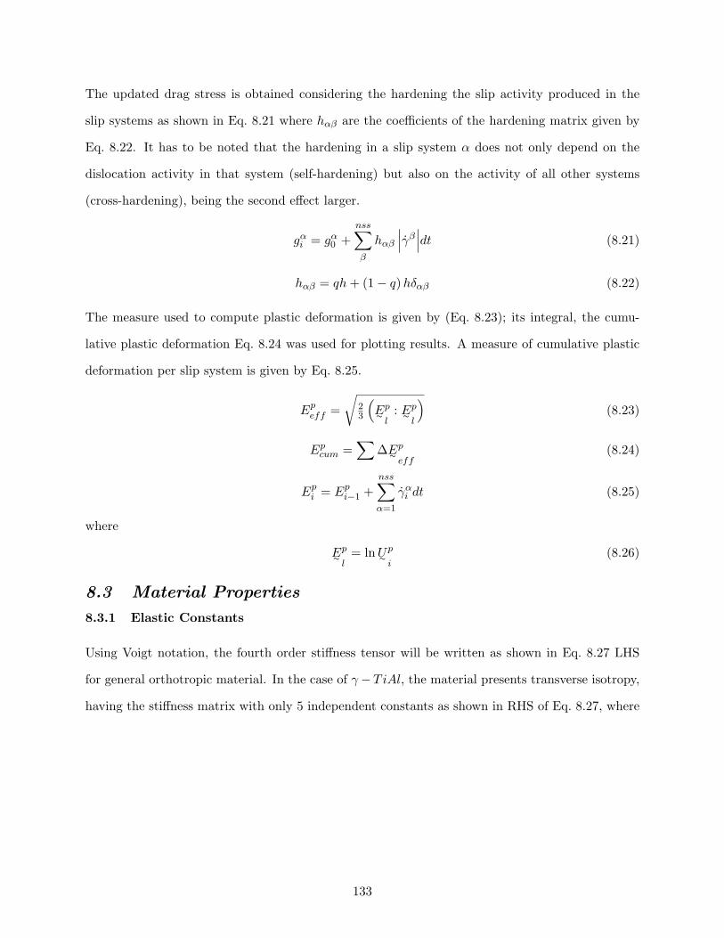
The updated drag stress is obtained considering the hardening the slip activity produced in the
slip systems as shown in Eq. 8.21 where hαβ are the coefficients of the hardening matrix given by
Eq. 8.22. It has to be noted that the hardening in a slip system α does not only depend on the
dislocation activity in that system (self-hardening) but also on the activity of all other systems
(cross-hardening), being the second effect larger.
gαi = gα
0 +nss∑β
hαβ
∣∣∣γβ∣∣∣dt (8.21)
hαβ = qh + (1− q) hδαβ (8.22)
The measure used to compute plastic deformation is given by (Eq. 8.23); its integral, the cumu-
lative plastic deformation Eq. 8.24 was used for plotting results. A measure of cumulative plastic
deformation per slip system is given by Eq. 8.25.
Epeff =
√23
(E∼
p
l: E∼
p
l
)(8.23)
Epcum =
∑∆E∼
p
eff(8.24)
Epi = Ep
i−1 +nss∑α=1
γαi dt (8.25)
where
E∼p
l= ln U∼
p
i(8.26)
8.3 Material Properties
8.3.1 Elastic Constants
Using Voigt notation, the fourth order stiffness tensor will be written as shown in Eq. 8.27 LHS
for general orthotropic material. In the case of γ−TiAl, the material presents transverse isotropy,
having the stiffness matrix with only 5 independent constants as shown in RHS of Eq. 8.27, where
133
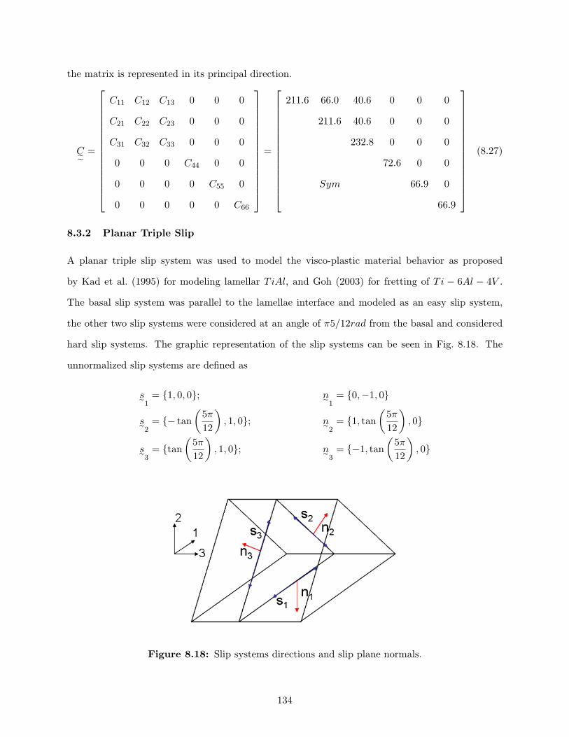
the matrix is represented in its principal direction.
C˜ =
C11 C12 C13 0 0 0
C21 C22 C23 0 0 0
C31 C32 C33 0 0 0
0 0 0 C44 0 0
0 0 0 0 C55 0
0 0 0 0 0 C66
=
211.6 66.0 40.6 0 0 0
211.6 40.6 0 0 0
232.8 0 0 0
72.6 0 0
Sym 66.9 0
66.9
(8.27)
8.3.2 Planar Triple Slip
A planar triple slip system was used to model the visco-plastic material behavior as proposed
by Kad et al. (1995) for modeling lamellar TiAl, and Goh (2003) for fretting of Ti − 6Al − 4V .
The basal slip system was parallel to the lamellae interface and modeled as an easy slip system,
the other two slip systems were considered at an angle of π5/12rad from the basal and considered
hard slip systems. The graphic representation of the slip systems can be seen in Fig. 8.18. The
unnormalized slip systems are defined as
s∼1
= 1, 0, 0; n∼1
= 0,−1, 0
s∼2
= − tan(
5π
12
), 1, 0; n∼
2= 1, tan
(5π
12
), 0
s∼3
= tan(
5π
12
), 1, 0; n∼
3= −1, tan
(5π
12
), 0
Figure 8.18: Slip systems directions and slip plane normals.
134
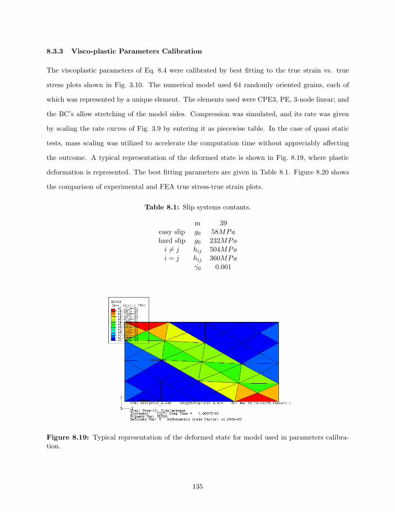
8.3.3 Visco-plastic Parameters Calibration
The viscoplastic parameters of Eq. 8.4 were calibrated by best fitting to the true strain vs. true
stress plots shown in Fig. 3.10. The numerical model used 64 randomly oriented grains, each of
which was represented by a unique element. The elements used were CPE3, PE, 3-node linear; and
the BC’s allow stretching of the model sides. Compression was simulated, and its rate was given
by scaling the rate curves of Fig. 3.9 by entering it as piecewise table. In the case of quasi static
tests, mass scaling was utilized to accelerate the computation time without appreciably affecting
the outcome. A typical representation of the deformed state is shown in Fig. 8.19, where plastic
deformation is represented. The best fitting parameters are given in Table 8.1. Figure 8.20 shows
the comparison of experimental and FEA true stress-true strain plots.
Table 8.1: Slip systems contants.
m 39easy slip g0 58MPahard slip g0 232MPa
i 6= j hij 504MPai = j hij 360MPa
γ0 0.001
Figure 8.19: Typical representation of the deformed state for model used in parameters calibra-tion.
135
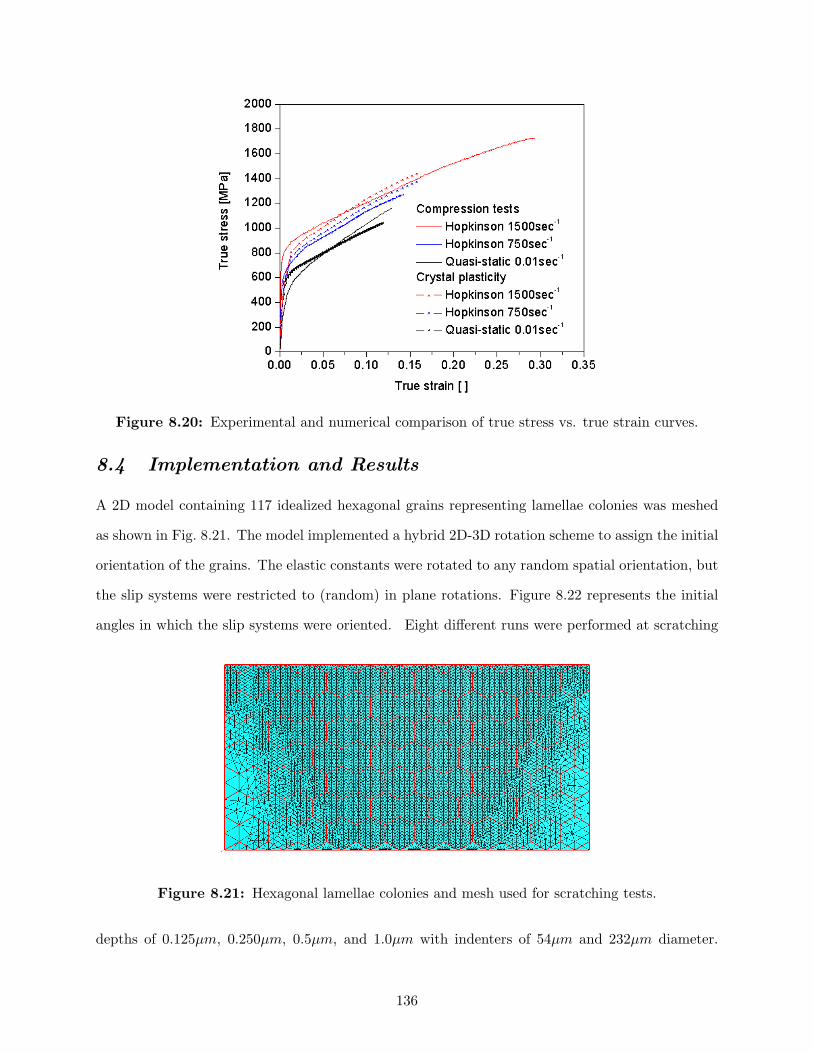
Figure 8.20: Experimental and numerical comparison of true stress vs. true strain curves.
8.4 Implementation and Results
A 2D model containing 117 idealized hexagonal grains representing lamellae colonies was meshed
as shown in Fig. 8.21. The model implemented a hybrid 2D-3D rotation scheme to assign the initial
orientation of the grains. The elastic constants were rotated to any random spatial orientation, but
the slip systems were restricted to (random) in plane rotations. Figure 8.22 represents the initial
angles in which the slip systems were oriented. Eight different runs were performed at scratching
Figure 8.21: Hexagonal lamellae colonies and mesh used for scratching tests.
depths of 0.125µm, 0.250µm, 0.5µm, and 1.0µm with indenters of 54µm and 232µm diameter.
136
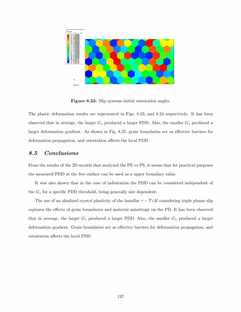
Figure 8.22: Slip systems initial orientation angles.
The plastic deformation results are represented in Figs. 8.23, and 8.24 respectively. It has been
observed that in average, the larger Gz produced a larger PDD. Also, the smaller Gz produced a
larger deformation gradient. As shown in Fig. 8.25, grain boundaries act as effective barriers for
deformation propagation, and orientation affects the local PDD.
8.5 Conclusions
From the results of the 2D models that analyzed the PE vs PS, it seems that for practical purposes
the measured PDD at the free surface can be used as a upper boundary value.
It was also shown that in the case of indentation the PDD can be considered independent of
the Gz for a specific PDD threshold, being generally size dependent.
The use of an idealized crystal plasticity of the lamellar γ − TiAl considering triple planar slip
captures the effects of grain boundaries and material anisotropy on the PD. It has been observed
that in average, the larger Gz produced a larger PDD. Also, the smaller Gz produced a larger
deformation gradient. Grain boundaries act as effective barriers for deformation propagation, and
orientation affects the local PDD.
137

Figure 8.23: Plastic deformation for small indenter. From top to bottom 0.125µm, 0.250µm,0.5µm, and 1µm penetration depth.
138
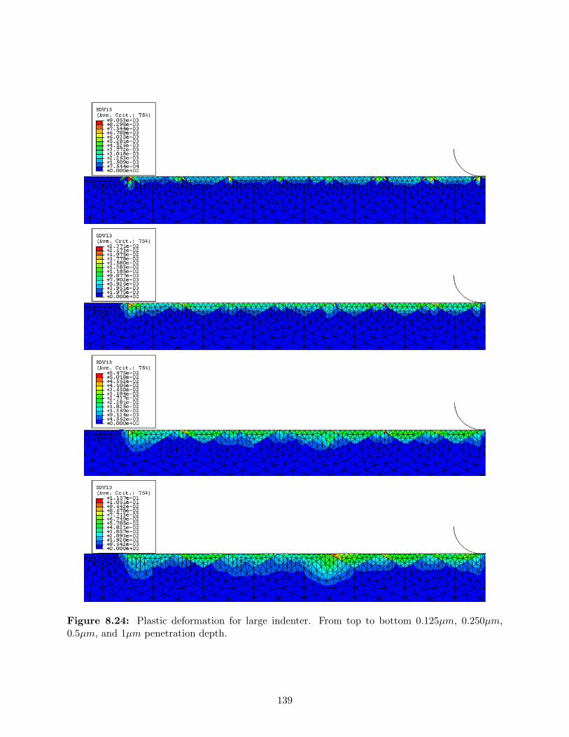
Figure 8.24: Plastic deformation for large indenter. From top to bottom 0.125µm, 0.250µm,0.5µm, and 1µm penetration depth.
139
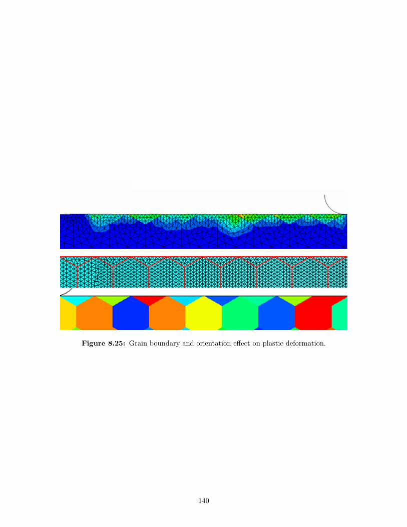
Figure 8.25: Grain boundary and orientation effect on plastic deformation.
140
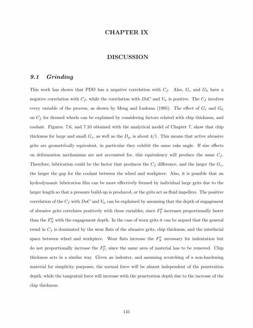
CHAPTER IX
DISCUSSION
9.1 Grinding
This work has shown that PDD has a negative correlation with Cf . Also, Gz and Gh have a
negative correlation with Cf , while the correlation with DoC and Vw is positive. The Cf involves
every variable of the process, as shown by Meng and Ludema (1995). The effect of Gz and Gh
on Cf for dressed wheels can be explained by considering factors related with chip thickness, and
coolant. Figures. 7.6, and 7.10 obtained with the analytical model of Chapter 7, show that chip
thickness for large and small Gz, as well as the Dg, is about 4/1. This means that active abrasive
grits are geometrically equivalent, in particular they exhibit the same rake angle. If size effects
on deformation mechanisms are not accounted for, this equivalency will produce the same Cf .
Therefore, lubrication could be the factor that produces the Cf difference, and the larger the Gz,
the larger the gap for the coolant between the wheel and workpiece. Also, it is possible that an
hydrodynamic lubrication film can be more effectively formed by individual large grits due to the
larger length so that a pressure build-up is produced, or the grits act as fluid impellers. The positive
correlation of the Cf with DoC and Vw can be explained by assuming that the depth of engagement
of abrasive grits correlates positively with these variables, since F ′′T increases proportionally faster
than the F ′′N with the engagement depth. In the case of worn grits it can be argued that the general
trend in Cf is dominated by the wear flats of the abrasive grits, chip thickness, and the interfacial
space between wheel and workpiece. Wear flats increase the F ′′N necessary for indentation but
do not proportionally increase the F ′′T , since the same area of material has to be removed. Chip
thickness acts in a similar way. Given an indenter, and assuming scratching of a non-hardening
material for simplicity purposes, the normal force will be almost independent of the penetration
depth, while the tangential force will increase with the penetration depth due to the increase of the
chip thickness.
141
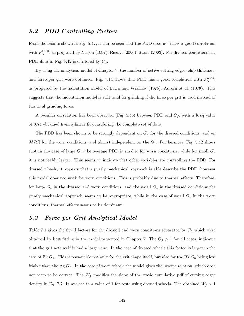
9.2 PDD Controlling Factors
From the results shown in Fig. 5.42, it can be seen that the PDD does not show a good correlation
with F ′N
0.5, as proposed by Nelson (1997); Razavi (2000); Stone (2003). For dressed conditions the
PDD data in Fig. 5.42 is clustered by Gz.
By using the analytical model of Chapter 7, the number of active cutting edges, chip thickness,
and force per grit were obtained. Fig. 7.14 shows that PDD has a good correlation with F ′′N
0.5,
as proposed by the indentation model of Lawn and Wilshaw (1975); Aurora et al. (1979). This
suggests that the indentation model is still valid for grinding if the force per grit is used instead of
the total grinding force.
A peculiar correlation has been observed (Fig. 5.45) between PDD and Cf , with a R-sq value
of 0.84 obtained from a linear fit considering the complete set of data.
The PDD has been shown to be strongly dependent on Gz for the dressed conditions, and on
MRR for the worn conditions, and almost independent on the Gz. Furthermore, Fig. 5.42 shows
that in the case of large Gz, the average PDD is smaller for worn conditions, while for small Gz
it is noticeably larger. This seems to indicate that other variables are controlling the PDD. For
dressed wheels, it appears that a purely mechanical approach is able describe the PDD; however
this model does not work for worn conditions. This is probably due to thermal effects. Therefore,
for large Gz in the dressed and worn conditions, and the small Gz in the dressed conditions the
purely mechanical approach seems to be appropriate, while in the case of small Gz in the worn
conditions, thermal effects seems to be dominant.
9.3 Force per Grit Analytical Model
Table 7.1 gives the fitted factors for the dressed and worn conditions separated by Gh which were
obtained by best fitting in the model presented in Chapter 7. The Gf > 1 for all cases, indicates
that the grit acts as if it had a larger size. In the case of dressed wheels this factor is larger in the
case of Bk Gh. This is reasonable not only for the grit shape itself, but also for the Bk Gh being less
friable than the Ag Gh. In the case of worn wheels the model gives the inverse relation, which does
not seem to be correct. The Wf modifies the slope of the static cumulative pdf of cutting edges
density in Eq. 7.7. It was set to a value of 1 for tests using dressed wheels. The obtained Wf > 1
142
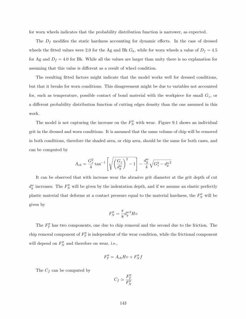
for worn wheels indicates that the probability distribution function is narrower, as expected.
The Df modifies the static hardness accounting for dynamic effects. In the case of dressed
wheels the fitted values were 2.0 for the Ag and Bk Gh, while for worn wheels a value of Df = 4.5
for Ag and Df = 4.0 for Bk. While all the values are larger than unity there is no explanation for
assuming that this value is different as a result of wheel condition.
The resulting fitted factors might indicate that the model works well for dressed conditions,
but that it breaks for worn conditions. This disagreement might be due to variables not accounted
for, such as temperature, possible contact of bond material with the workpiece for small Gz, or
a different probability distribution function of cutting edges density than the one assumed in this
work.
The model is not capturing the increase on the F ′′N with wear. Figure 9.1 shows an individual
grit in the dressed and worn conditions. It is assumed that the same volume of chip will be removed
in both conditions, therefore the shaded area, or chip area, should be the same for both cases, and
can be computed by
Ach =G2
z
4tan−1
[√(Gz
dwg
)2
− 1
]−
dwg
4
√G2
z − dwg
2
It can be observed that with increase wear the abrasive grit diameter at the grit depth of cut
dwg increases. The F ′′
N will be given by the indentation depth, and if we assume an elastic perfectly
plastic material that deforms at a contact pressure equal to the material hardness, the F ′′N will be
given by
F ′′N =
π
8dw
g2Hv
The F ′′T has two components, one due to chip removal and the second due to the friction. The
chip removal component of F ′′T is independent of the wear condition, while the frictional component
will depend on F ′′N and therefore on wear, i.e.,
F ′′T = AchHv + F ′′
Nf
The Cf can be computed by
Cf 'F ′′
T
F ′′N
143
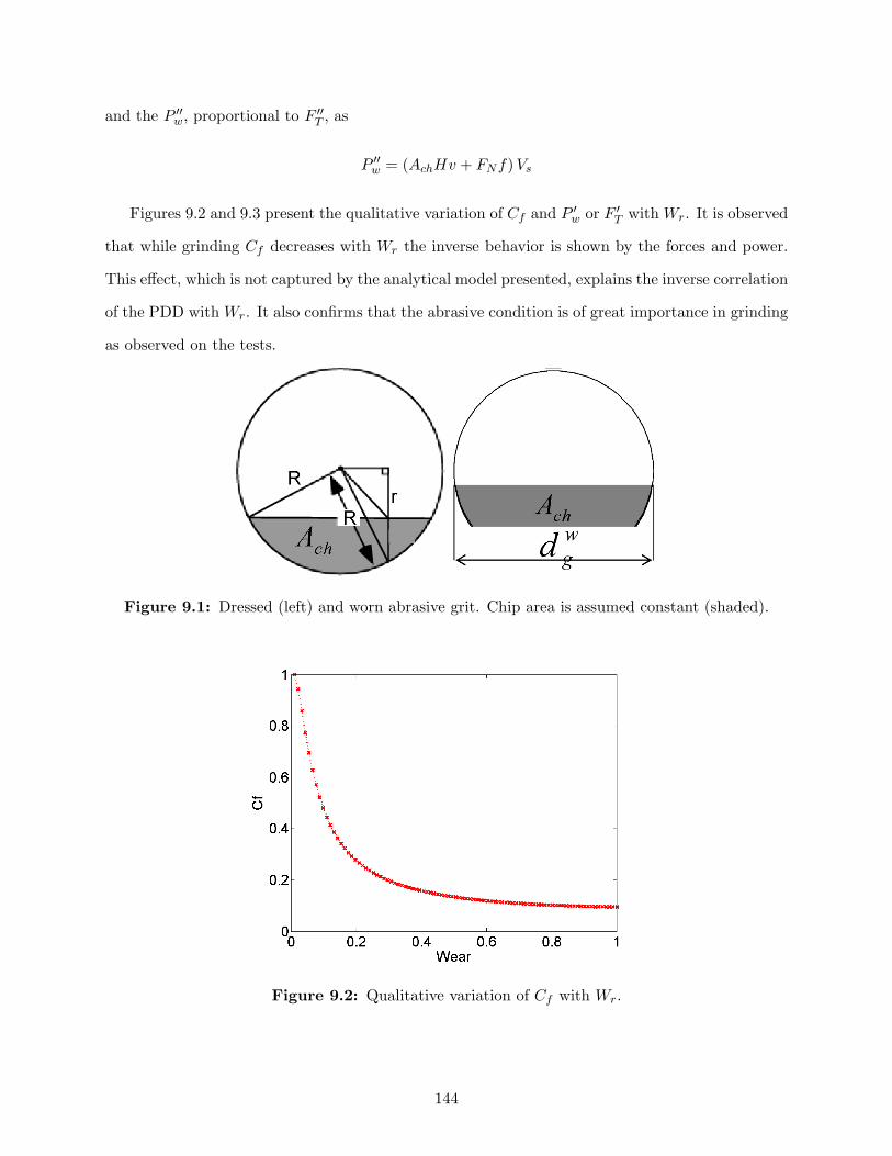
and the P ′′w, proportional to F ′′
T , as
P ′′w = (AchHv + FNf) Vs
Figures 9.2 and 9.3 present the qualitative variation of Cf and P ′w or F ′
T with Wr. It is observed
that while grinding Cf decreases with Wr the inverse behavior is shown by the forces and power.
This effect, which is not captured by the analytical model presented, explains the inverse correlation
of the PDD with Wr. It also confirms that the abrasive condition is of great importance in grinding
as observed on the tests.
Figure 9.1: Dressed (left) and worn abrasive grit. Chip area is assumed constant (shaded).
Figure 9.2: Qualitative variation of Cf with Wr.
144
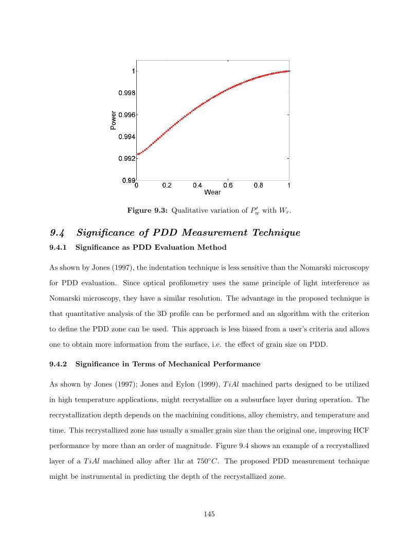
Figure 9.3: Qualitative variation of P ′w with Wr.
9.4 Significance of PDD Measurement Technique
9.4.1 Significance as PDD Evaluation Method
As shown by Jones (1997), the indentation technique is less sensitive than the Nomarski microscopy
for PDD evaluation. Since optical profilometry uses the same principle of light interference as
Nomarski microscopy, they have a similar resolution. The advantage in the proposed technique is
that quantitative analysis of the 3D profile can be performed and an algorithm with the criterion
to define the PDD zone can be used. This approach is less biased from a user’s criteria and allows
one to obtain more information from the surface, i.e. the effect of grain size on PDD.
9.4.2 Significance in Terms of Mechanical Performance
As shown by Jones (1997); Jones and Eylon (1999), TiAl machined parts designed to be utilized
in high temperature applications, might recrystallize on a subsurface layer during operation. The
recrystallization depth depends on the machining conditions, alloy chemistry, and temperature and
time. This recrystallized zone has usually a smaller grain size than the original one, improving HCF
performance by more than an order of magnitude. Figure 9.4 shows an example of a recrystallized
layer of a TiAl machined alloy after 1hr at 750C. The proposed PDD measurement technique
might be instrumental in predicting the depth of the recrystallized zone.
145
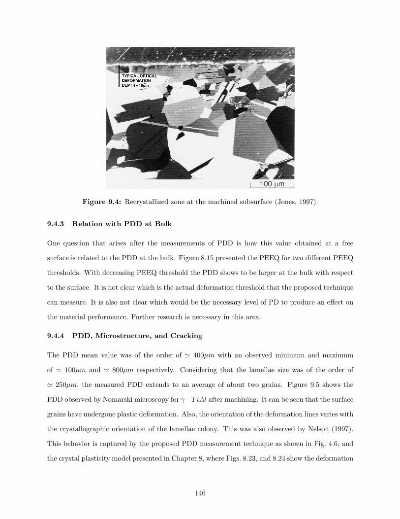
Figure 9.4: Recrystallized zone at the machined subsurface (Jones, 1997).
9.4.3 Relation with PDD at Bulk
One question that arises after the measurements of PDD is how this value obtained at a free
surface is related to the PDD at the bulk. Figure 8.15 presented the PEEQ for two different PEEQ
thresholds. With decreasing PEEQ threshold the PDD shows to be larger at the bulk with respect
to the surface. It is not clear which is the actual deformation threshold that the proposed technique
can measure. It is also not clear which would be the necessary level of PD to produce an effect on
the material performance. Further research is necessary in this area.
9.4.4 PDD, Microstructure, and Cracking
The PDD mean value was of the order of ' 400µm with an observed minimum and maximum
of ' 100µm and ' 800µm respectively. Considering that the lamellae size was of the order of
' 250µm, the measured PDD extends to an average of about two grains. Figure 9.5 shows the
PDD observed by Nomarski microscopy for γ−TiAl after machining. It can be seen that the surface
grains have undergone plastic deformation. Also, the orientation of the deformation lines varies with
the crystallographic orientation of the lamellae colony. This was also observed by Nelson (1997).
This behavior is captured by the proposed PDD measurement technique as shown in Fig. 4.6, and
the crystal plasticity model presented in Chapter 8, where Figs. 8.23, and 8.24 show the deformation
146
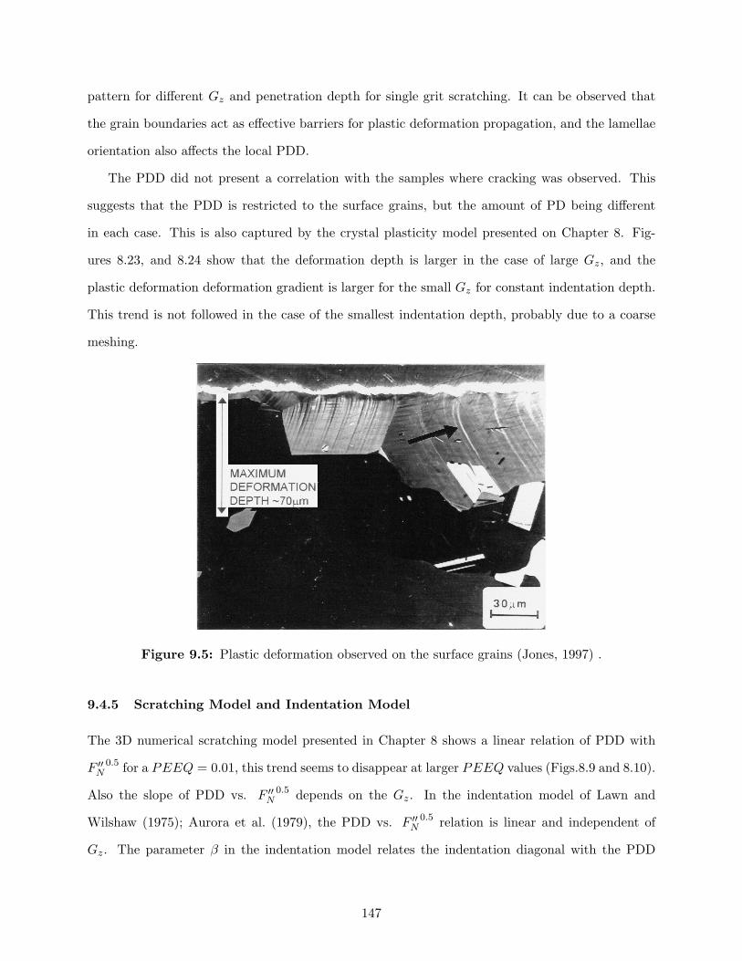
pattern for different Gz and penetration depth for single grit scratching. It can be observed that
the grain boundaries act as effective barriers for plastic deformation propagation, and the lamellae
orientation also affects the local PDD.
The PDD did not present a correlation with the samples where cracking was observed. This
suggests that the PDD is restricted to the surface grains, but the amount of PD being different
in each case. This is also captured by the crystal plasticity model presented on Chapter 8. Fig-
ures 8.23, and 8.24 show that the deformation depth is larger in the case of large Gz, and the
plastic deformation deformation gradient is larger for the small Gz for constant indentation depth.
This trend is not followed in the case of the smallest indentation depth, probably due to a coarse
meshing.
Figure 9.5: Plastic deformation observed on the surface grains (Jones, 1997) .
9.4.5 Scratching Model and Indentation Model
The 3D numerical scratching model presented in Chapter 8 shows a linear relation of PDD with
F ′′N
0.5 for a PEEQ = 0.01, this trend seems to disappear at larger PEEQ values (Figs.8.9 and 8.10).
Also the slope of PDD vs. F ′′N
0.5 depends on the Gz. In the indentation model of Lawn and
Wilshaw (1975); Aurora et al. (1979), the PDD vs. F ′′N
0.5 relation is linear and independent of
Gz. The parameter β in the indentation model relates the indentation diagonal with the PDD
147
depth. Nevertheless, this parameter is loosely defined since the definition of the PDD depends on
the experimental technique. The parameter β may take a range of values and the linearity of PDD
with F ′′N
0.5 might not be observed for the range. The dependence of PDD with Gz for a constant
load is observed for 2D modeling of indentation as shown in Fig. 8.16. The PDD can be considered
independent of the Gz only at a particular deformation threshold. Size dependence is also seen for
simulations of 3D scratching.
From the 3D numerical scratching model it can also be seen that a single scratching pass
produces a PDD of approximately an order of magnitude smaller than the ones measured. A
probable cause for this is that the deformation history due to successive scratching in grinding is
not accounted for in the model.
9.5 Residual Stress
Two different types of x-ray scans were used to acquire data: the so-called detector scan, and Ψ
scans. In the detector scan the azimuth angle of the x-ray changes for the different conditions,
thereby changing the beam penetration depth. In the case of presence of step stress gradients on
the specimen the hypothesis of uniform stress in the measured region would be violated. In the
case of Φ scans the azimuth angle is kept constant, obtaining different measurements at different
Φ angles. The disadvantage of this method is that the measured interplanar distances are close to
each other, and errors are amplified.
148
CHAPTER X
CONCLUSIONS AND RECOMMENDATIONS
10.1 Conclusions
10.1.1 PDD Evaluation Technique
The PDD evaluation method proposed, combines the quantitative capabilities of the microhardness
measurement with the sensitivity of Nomarski microscopy. Quantitative analysis of the surface can
be performed and an algorithm with the criterion to define the PDD zone can be used. This
approach is less biased from the user’s experience.
The method can be used to obtain a unique parameter for PDD or a complete mapping of the
surface, according to the data analysis performed.
The averaging method of determining PDD is based on averaging the out-of-planarity of lines
parallel to the surface. This method gives a unique value for PDD and is robust with respect to
missing points and surface finishing.
The contour plot method allows the computation of PDD variability with respect to grain
morphology and material anisotropy. Since no data averaging takes place, this method is very
sensitive to surface finishing.
The practical limitation of these methods is given by the quality of surface preparation, e.g. the
surface roughness is more important than its waviness. With a surface roughness of Ra < 1µm it
has been possible to work with an out-of-planarity threshold of 1µm, thereby obtaining consistent
results between replications and analysis techniques. An out-of-planarity threshold of 0.25µm has
been of limited applicability for the present work.
10.1.2 Grinding
It has been observed that grinding is very sensitive to wheel conditioning and wear. Complete
truing and dressing conditions should be specified to obtain consistent results. Cooling conditions
are also important.
149
10.1.2.1 Plastic Deformation
The PDD mean value was of the order of ' 400µm with an observed minimum and maximum
of ' 100µm and ' 800µm respectively. Considering that the lamellae size was of the order of
' 250µm, the measured PDD extends on an average of about two grains.
It has been observed that for dressed conditions the PDD strongly depends on Gz. The PDD
mean and standard deviation for small and large Gz is 186± 40µm, and 543± 85µm respectively.
Most of the PDD variance can be explained by the Gz factor alone, Vw being not a relevant factor.
There is some influence of the Gh, and the interactions between Gz and Gh; and Gz and DoC. The
R-Sq value for the model PDD[µm] = 78.1 + 2.007GS is 87.9%.
In the case of worn conditions the PDD strongly depends on DoC and Vw, therefore MRR also
correlates with PDD. The DoC explains half of the data variance followed in importance by Vw.
Even considering most of the controlled variables and their interaction in a linear model, the R-Sq
value was less than 0.82. The PDD mean and standard deviation was of 407 ± 120µm for worn
wheels and 365± 191µm for dressed ones.
The change in behavior from dressed to worn conditions is believed to be produced by the
increase of thermal effects and force per abrasive grit due to wear flats.
In the case of large Gz it has been observed that the PDD decreases with Wr while the inverse
behavior was observed for small Gz. While the P ′w was of the same order of magnitude for large
Gz for worn and dressed conditions, it increased an average of 6 times for small Gz. This would
indicate that for large Gz the thermal effects were not very different for the two Wr conditions and
the PDD was determined by the Gz. The decrease of the PDD could be explained by assuming
that the worn wheel presented a narrower distribution of cutting edges than the dressed one. This
could be due to some fracture of the abrasive grits during the first stages of grinding after dressing,
which results as if having a smaller grit size. In the case of small Gz, it can be assumed that the
generation of wear flats increased the force per abrasive grit and temperature with the consequent
increase of the PDD.
It has been observed that the PDD is inversely correlated to the Cf . A R-sq value of 0.84 is
obtained by a linear fit of PDD with Cf .
150
10.1.2.2 Grinding Friction Coefficient
Grit size and shape have a negative correlation with Cf , while the correlation with DoC and Vw
is positive. In the case of worn wheels all individual factors, and the interactions between Gz and
the rest of the variables are relevant for Cf , and their correlation is inverse to the one shown for
PDD. While the Cf trend with Gz and Gh is the same as with dressed wheels, the dependence on
DoC, and Vw is inverse. The negative correlation of the Cf with DoC and Vw can be explained by
considering the shape change in the abrasives with Wr.
10.1.2.3 Specific Normal Force
In the case of dressed wheels, F ′N has a positive correlation with all the individual factors, and the
Gz and Gh interaction.
In the case of dressed wheels, all individual factors and Gz and DoC; and DoC and Vw inter-
actions are relevant for F ′N . Unlike the case of dressed wheels, Gz has a negative correlation with
F ′N , which can be explained by assuming that the relative wear flat in the small grit is larger than
in the large grit. This can be due to the fact that poorer lubrication conditions might occur with
smaller grits, and therefore higher temperatures increase the wear rate of the diamond.
10.1.2.4 Surface Parameters
It was observed that the Ra and BA mean values increased with wear. This was probably due to
the effect of plowing in the formation of side ridges.
For the dressed conditions, the mean Ra value is in the range of 0.4µm to 0.7µm, and the mean
90% BA of 3.9µm, Gz being is the most relevant factor.
For the worn conditions, the mean Ra value is in the range of 0.65µm to 0.95µm, with a mean
value for 90% BA of 5.7µm, Gz being the most relevant variable.
10.1.2.5 Cracking
The PDD was not correlated with cracking, as might be expected before the present work.
No cracking was observed on the ground surface under a magnification of 60X for dressed
wheels.
151
Surface cracking was observed on tests using worn wheels for small Gz in the 4 treatments with
the largest MRR. This cracking appears to be due to thermal effects and it was not related to
PDD. It has been observed that cracking was produced on treatments with high F ′N , or high P ′
w
and low Cf .
Surface cracking was observed on tests using worn wheels, for the Ag8 and Bk8 treatments. It
was also observed for the large Gz for the Bk2 treatment, and only one crack in a sample with
Ag2 treatment. While extensive cracking was observed in the Bk2 treatment, only a single crack
was observed in the Ag2 case. The Ag Gh presents a higher Cf than the Bk, due to its angular
shape and higher friability with respect to the Bk. Wear flats on Bk shape abrasive grits increase
redundant work and heat generation, decreasing Cf .
10.1.3 Residual Stresses
Residual stresses were measured in 4 ground samples analyzing the effect of a high and low PDD
value. It can be seen that compressive stresses are close to the GPa on the surface.
Numerous experimental difficulties produced a high variance of the results and the impossibility
to obtain results in zones of apparently high stress gradients.
10.1.4 Analytical Modeling
By use of the analytical model of the number of active cutting edges, chip thickness, and force
per grit were obtained, and the PDD has shown a good correlation with F ′′N
0.5, as proposed by
the indentation model of Lawn and Wilshaw (1975); Aurora et al. (1979). This suggests that the
indentation model is still valid for grinding if the force per grit is used instead of the total grinding
force.
The model captures the difference in the number of cutting edges and chip thickness for the
different Gz.
The resulting fitted factors of the analytical model might indicate that the model works well for
dressed conditions by capturing expected trends, but it breaks for worn conditions. This disagree-
ment might be due to variables not accounted for such as temperature, possible contact of bond
material with the workpiece for small Gz, or a different probability density function of the cutting
edges density than the one assumed in this work.
152
The analytical model predicts for the dressed conditions a cutting edge density of the order of
3#/mm2 to 6#/mm2 for small Gz, and less than 0.5#/mm2 for large Gz. Model and test P ′w and
forces are in reasonable agreement, but in some cases all these values differ by a factor of 2.
Chip thickness is of the order of 2.1µm to 4.5µm for large Gz, and in the order of 0.5µm to
1.1µm for small Gz. These values are in agreement with the ones found in the literature.
The analytical model predicts for the worn conditions that the cutting edge density is of the
order of 4#/mm2 to 8#/mm2 for small Gz, and less than 0.6#/mm2 for large Gz. Chip thickness
is of the order of 1.5µm to 3.2µm for large Gz, and in the order of 0.2µm to 0.7µm for small Gz.
As expected these values are smaller than the ones found for dressed wheels.
The resulting fitted factors of the analytical model might indicate that the model works well
for dressed conditions by capturing expected trends, but it does not give good predictions for worn
conditions. This disagreement might be due to variables not accounted for such as temperature,
possible contact of bond material with the workpiece for small Gz, or a different probability density
function of the cutting edges density than the one assumed in this work.
10.1.5 Numerical Modeling
From the results of the 2D models that analyzed the PE vs PS, it seems that for practical purposes
the measured PDD at the free surface can be used as a upper boundary value.
It was also shown that in the case of indentation the PDD can be considered independent of
the Gz for a specific PDD threshold, being generally size dependent.
The use of an idealized crystal plasticity of the lamellar γ − TiAl considering triple planar slip
captures the effects of grain boundaries and material anisotropy on the PD. It has been observed
that in average, the larger Gz produced a larger PDD. Also the smaller Gz produced a larger
deformation gradient. Grain boundaries act as effective barriers for deformation propagation, and
orientation affects the local PDD.
10.2 Recommendations
Further characterization of the deformed zone may include not only the PDD, as in the present
work, but also the first and second derivatives of the out-of-planarity profile shown in Fig. 4.6, and
their relation to cracking.
153
Two relevant factors were left for modeling in future work: thermal effects, and deformation
history. While thermal effects can be added with state-of-the-art FEA, the implementation of
models that account for history effects under localized loads under large sliding and deformation
conditions presents some difficulties. Finite element codes working in an Eulerian framework might
be instrumental for these purposes.
The crystal plasticity model has shown that grain boundaries act as effective barriers for PD. An
implementation of random grain sizes and geometry by use of Voronoi tesselation would be useful
to further analyze the deformation dependence on these variables and approximate the model to
the actual test.
Other modeling improvements might include the addition of more slip systems, explicit modeling
of the two phases, improved hardening modeling, consideration of time dependent properties per
slip system, fracture and fatigue modeling, actual abrasive shape, and 3D geometry.
One of the possible reasons for the departure of the force per grit model from the tests can be
related to the use of an incorrect probability density function of the cutting edges to describe the
wheel surface. The use of replicas and the work and errors associated with them can be avoided
if modifications are introduced to present generation of 3D profilometers by designing the devices
with similar stage capabilities as metallurgical microscopes, giving room for a grinding wheel to fit
in the instrument. The inconvenience of dismounting the wheel from the grinder and later truing
processes is a minor one compared with the benefits of direct measurement.
The RS analysis technique can be improved by considering the radiation attenuation in the
subsurface, and stress gradients (Suominen and Carr, 1999; Behnken and Hauk, 2001; Ely et al.,
1999; Wern, 1999; Zhu et al., 1995)
The measurement of residual stresses with neutron diffraction can be used to improve the
resolution of the stress at the surface of highly deformed material, and to avoid the artifacts
introduced by the layer removal technique, since the penetration depth of the radiation is of the
order of millimeters.
Machined parts designed to be utilized in high temperature applications might recrystallize
on a subsurface layer during operation. The recrystallization depth depends on the machining
conditions, alloy chemistry, temperature and time. A further correlation of the proposed PDD
154
measurement technique with the recrystallized depth would be of interest.
One question that arises after the measurements of PDD is how this value obtained at a free
surface is related to the PDD at the bulk. With decreasing PEEQ threshold the PDD shows to
be larger at the bulk with respect to the surface. It is not clear which is the actual deformation
threshold that the proposed technique can measure. It is also not clear which would be the necessary
level of PD to produce an effect on the material performance. Further research is necessary in this
area.
155

APPENDIX A
GRINDING EXPERIMENTAL RESULTS
156
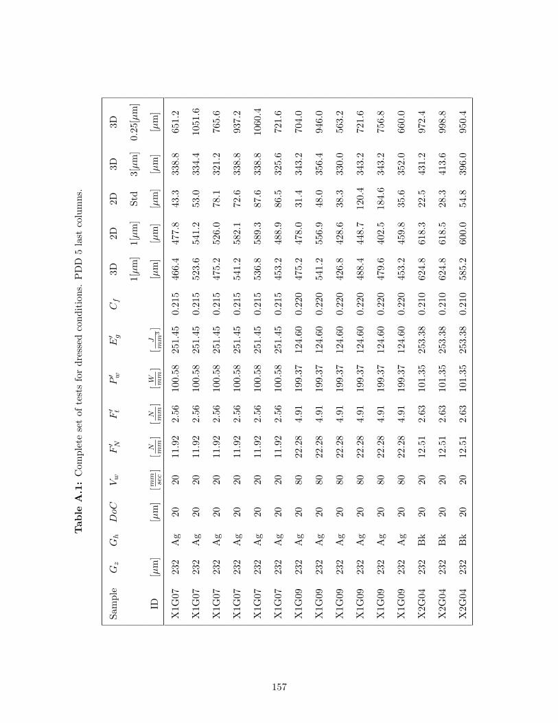
Tab
leA
.1:
Com
plet
ese
tof
test
sfo
rdr
esse
dco
ndit
ions
.P
DD
5la
stco
lum
ns.
Sam
ple
Gz
Gh
DoC
Vw
F′ N
F′ t
P′ w
E′ g
Cf
3D2D
2D3D
3D
1[µm
]1[
µm
]St
d3[
µm
]0.
25[µ
m]
ID[µ
m]
[µm
][m
mse
c]
[N mm
][
N mm
][
W mm
][
Jm
m3]
[µm
][µ
m]
[µm
][µ
m]
[µm
]
X1G
0723
2A
g20
2011
.92
2.56
100.
5825
1.45
0.21
546
6.4
477.
843
.333
8.8
651.
2
X1G
0723
2A
g20
2011
.92
2.56
100.
5825
1.45
0.21
552
3.6
541.
253
.033
4.4
1051
.6
X1G
0723
2A
g20
2011
.92
2.56
100.
5825
1.45
0.21
547
5.2
526.
078
.132
1.2
765.
6
X1G
0723
2A
g20
2011
.92
2.56
100.
5825
1.45
0.21
554
1.2
582.
172
.633
8.8
937.
2
X1G
0723
2A
g20
2011
.92
2.56
100.
5825
1.45
0.21
553
6.8
589.
387
.633
8.8
1060
.4
X1G
0723
2A
g20
2011
.92
2.56
100.
5825
1.45
0.21
545
3.2
488.
986
.532
5.6
721.
6
X1G
0923
2A
g20
8022
.28
4.91
199.
3712
4.60
0.22
047
5.2
478.
031
.434
3.2
704.
0
X1G
0923
2A
g20
8022
.28
4.91
199.
3712
4.60
0.22
054
1.2
556.
948
.035
6.4
946.
0
X1G
0923
2A
g20
8022
.28
4.91
199.
3712
4.60
0.22
042
6.8
428.
638
.333
0.0
563.
2
X1G
0923
2A
g20
8022
.28
4.91
199.
3712
4.60
0.22
048
8.4
448.
712
0.4
343.
272
1.6
X1G
0923
2A
g20
8022
.28
4.91
199.
3712
4.60
0.22
047
9.6
402.
518
4.6
343.
275
6.8
X1G
0923
2A
g20
8022
.28
4.91
199.
3712
4.60
0.22
045
3.2
459.
835
.635
2.0
660.
0
X2G
0423
2B
k20
2012
.51
2.63
101.
3525
3.38
0.21
062
4.8
618.
322
.543
1.2
972.
4
X2G
0423
2B
k20
2012
.51
2.63
101.
3525
3.38
0.21
062
4.8
618.
528
.341
3.6
998.
8
X2G
0423
2B
k20
2012
.51
2.63
101.
3525
3.38
0.21
058
5.2
600.
054
.839
6.0
950.
4
157
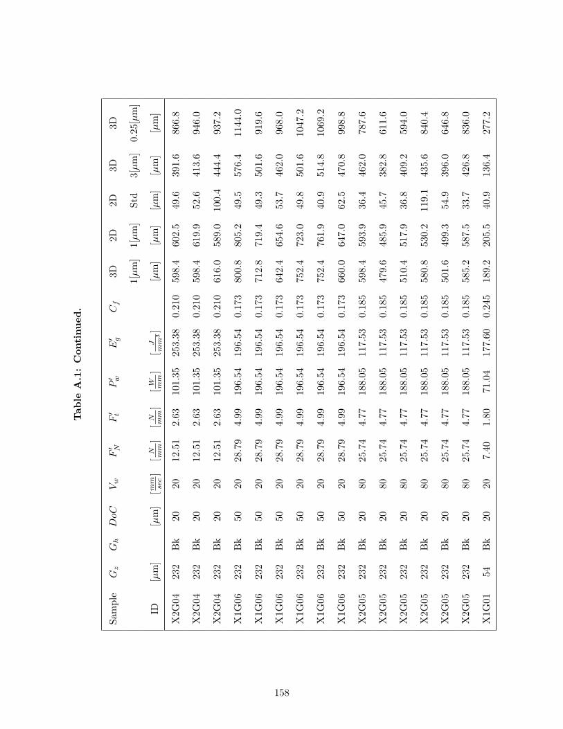
Tab
leA
.1:
Con
tinued
.
Sam
ple
Gz
Gh
DoC
Vw
F′ N
F′ t
P′ w
E′ g
Cf
3D2D
2D3D
3D
1[µm
]1[
µm
]St
d3[
µm
]0.
25[µ
m]
ID[µ
m]
[µm
][m
mse
c]
[N mm
][
N mm
][
W mm
][
Jm
m3]
[µm
][µ
m]
[µm
][µ
m]
[µm
]
X2G
0423
2B
k20
2012
.51
2.63
101.
3525
3.38
0.21
059
8.4
602.
549
.639
1.6
866.
8
X2G
0423
2B
k20
2012
.51
2.63
101.
3525
3.38
0.21
059
8.4
619.
952
.641
3.6
946.
0
X2G
0423
2B
k20
2012
.51
2.63
101.
3525
3.38
0.21
061
6.0
589.
010
0.4
444.
493
7.2
X1G
0623
2B
k50
2028
.79
4.99
196.
5419
6.54
0.17
380
0.8
805.
249
.557
6.4
1144
.0
X1G
0623
2B
k50
2028
.79
4.99
196.
5419
6.54
0.17
371
2.8
719.
449
.350
1.6
919.
6
X1G
0623
2B
k50
2028
.79
4.99
196.
5419
6.54
0.17
364
2.4
654.
653
.746
2.0
968.
0
X1G
0623
2B
k50
2028
.79
4.99
196.
5419
6.54
0.17
375
2.4
723.
049
.850
1.6
1047
.2
X1G
0623
2B
k50
2028
.79
4.99
196.
5419
6.54
0.17
375
2.4
761.
940
.951
4.8
1069
.2
X1G
0623
2B
k50
2028
.79
4.99
196.
5419
6.54
0.17
366
0.0
647.
062
.547
0.8
998.
8
X2G
0523
2B
k20
8025
.74
4.77
188.
0511
7.53
0.18
559
8.4
593.
936
.446
2.0
787.
6
X2G
0523
2B
k20
8025
.74
4.77
188.
0511
7.53
0.18
547
9.6
485.
945
.738
2.8
611.
6
X2G
0523
2B
k20
8025
.74
4.77
188.
0511
7.53
0.18
551
0.4
517.
936
.840
9.2
594.
0
X2G
0523
2B
k20
8025
.74
4.77
188.
0511
7.53
0.18
558
0.8
530.
211
9.1
435.
684
0.4
X2G
0523
2B
k20
8025
.74
4.77
188.
0511
7.53
0.18
550
1.6
499.
354
.939
6.0
646.
8
X2G
0523
2B
k20
8025
.74
4.77
188.
0511
7.53
0.18
558
5.2
587.
533
.742
6.8
836.
0
X1G
0154
Bk
2020
7.40
1.80
71.0
417
7.60
0.24
518
9.2
205.
540
.913
6.4
277.
2
158
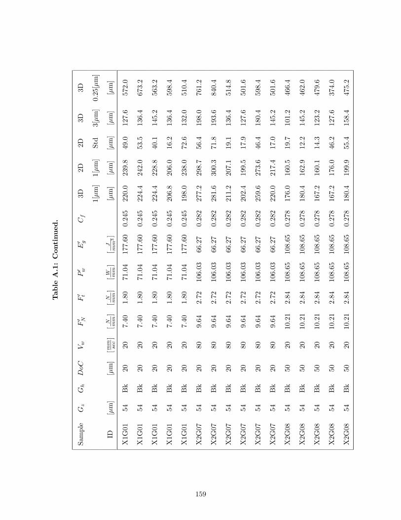
Tab
leA
.1:
Con
tinued
.
Sam
ple
Gz
Gh
DoC
Vw
F′ N
F′ t
P′ w
E′ g
Cf
3D2D
2D3D
3D
1[µm
]1[
µm
]St
d3[
µm
]0.
25[µ
m]
ID[µ
m]
[µm
][m
mse
c]
[N mm
][
N mm
][
W mm
][
Jm
m3]
[µm
][µ
m]
[µm
][µ
m]
[µm
]
X1G
0154
Bk
2020
7.40
1.80
71.0
417
7.60
0.24
522
0.0
239.
849
.012
7.6
572.
0
X1G
0154
Bk
2020
7.40
1.80
71.0
417
7.60
0.24
522
4.4
242.
053
.513
6.4
673.
2
X1G
0154
Bk
2020
7.40
1.80
71.0
417
7.60
0.24
522
4.4
228.
840
.114
5.2
563.
2
X1G
0154
Bk
2020
7.40
1.80
71.0
417
7.60
0.24
520
6.8
206.
016
.213
6.4
598.
4
X1G
0154
Bk
2020
7.40
1.80
71.0
417
7.60
0.24
519
8.0
238.
072
.613
2.0
510.
4
X2G
0754
Bk
2080
9.64
2.72
106.
0366
.27
0.28
227
7.2
298.
756
.419
8.0
761.
2
X2G
0754
Bk
2080
9.64
2.72
106.
0366
.27
0.28
228
1.6
300.
371
.819
3.6
840.
4
X2G
0754
Bk
2080
9.64
2.72
106.
0366
.27
0.28
221
1.2
207.
119
.113
6.4
514.
8
X2G
0754
Bk
2080
9.64
2.72
106.
0366
.27
0.28
220
2.4
199.
517
.912
7.6
501.
6
X2G
0754
Bk
2080
9.64
2.72
106.
0366
.27
0.28
225
9.6
273.
646
.418
0.4
598.
4
X2G
0754
Bk
2080
9.64
2.72
106.
0366
.27
0.28
222
0.0
217.
417
.014
5.2
501.
6
X2G
0854
Bk
5020
10.2
12.
8410
8.65
108.
650.
278
176.
016
0.5
19.7
101.
246
6.4
X2G
0854
Bk
5020
10.2
12.
8410
8.65
108.
650.
278
180.
416
2.9
12.2
145.
246
2.0
X2G
0854
Bk
5020
10.2
12.
8410
8.65
108.
650.
278
167.
216
0.1
14.3
123.
247
9.6
X2G
0854
Bk
5020
10.2
12.
8410
8.65
108.
650.
278
167.
217
6.0
46.2
127.
637
4.0
X2G
0854
Bk
5020
10.2
12.
8410
8.65
108.
650.
278
180.
419
9.9
55.4
158.
447
5.2
159
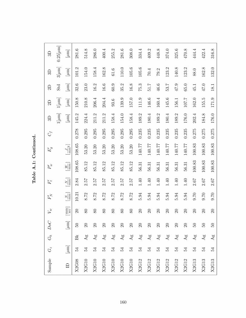
Tab
leA
.1:
Con
tinued
.
Sam
ple
Gz
Gh
DoC
Vw
F′ N
F′ t
P′ w
E′ g
Cf
3D2D
2D3D
3D
1[µm
]1[
µm
]St
d3[
µm
]0.
25[µ
m]
ID[µ
m]
[µm
][m
mse
c]
[N mm
][
N mm
][
W mm
][
Jm
m3]
[µm
][µ
m]
[µm
][µ
m]
[µm
]
X2G
0854
Bk
5020
10.2
12.
8410
8.65
108.
650.
278
145.
215
0.8
32.6
101.
228
1.6
X2G
1054
Ag
2080
8.72
2.57
85.1
253
.20
0.29
522
4.4
210.
823
.015
4.0
514.
8
X2G
1054
Ag
2080
8.72
2.57
85.1
253
.20
0.29
521
1.2
206.
416
.215
8.4
286.
0
X2G
1054
Ag
2080
8.72
2.57
85.1
253
.20
0.29
521
1.2
204.
416
.616
2.8
400.
4
X2G
1054
Ag
2080
8.72
2.57
85.1
253
.20
0.29
515
8.4
93.6
60.9
61.6
255.
2
X2G
1054
Ag
2080
8.72
2.57
85.1
253
.20
0.29
515
4.0
139.
935
.211
0.0
281.
6
X2G
1054
Ag
2080
8.72
2.57
85.1
253
.20
0.29
515
8.4
157.
016
.810
5.6
308.
0
X2G
1254
Ag
2020
5.94
1.40
56.3
114
0.77
0.23
518
9.2
111.
975
.310
5.6
334.
4
X2G
1254
Ag
2020
5.94
1.40
56.3
114
0.77
0.23
518
0.4
146.
651
.770
.440
9.2
X2G
1254
Ag
2020
5.94
1.40
56.3
114
0.77
0.23
518
9.2
160.
446
.679
.244
8.8
X2G
1254
Ag
2020
5.94
1.40
56.3
114
0.77
0.23
518
0.4
145.
653
.712
3.2
374.
0
X2G
1254
Ag
2020
5.94
1.40
56.3
114
0.77
0.23
518
9.2
156.
147
.914
0.8
325.
6
X2G
1254
Ag
2020
5.94
1.40
56.3
114
0.77
0.23
517
6.0
107.
765
.012
3.2
470.
8
X2G
1354
Ag
5020
9.70
2.67
100.
8310
0.83
0.27
520
2.4
162.
045
.188
.044
4.4
X2G
1354
Ag
5020
9.70
2.67
100.
8310
0.83
0.27
518
4.8
155.
547
.016
2.8
422.
4
X2G
1354
Ag
5020
9.70
2.67
100.
8310
0.83
0.27
517
6.0
171.
918
.113
2.0
316.
8
160
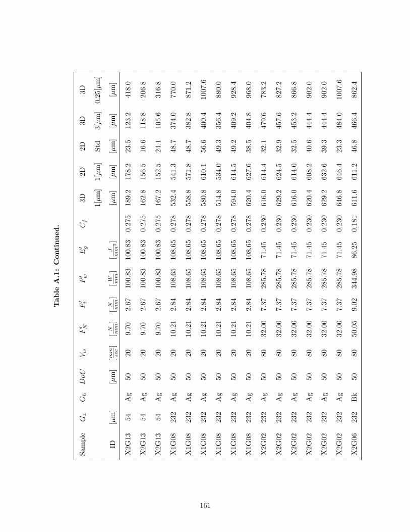
Tab
leA
.1:
Con
tinued
.
Sam
ple
Gz
Gh
DoC
Vw
F′ N
F′ t
P′ w
E′ g
Cf
3D2D
2D3D
3D
1[µm
]1[
µm
]St
d3[
µm
]0.
25[µ
m]
ID[µ
m]
[µm
][m
mse
c]
[N mm
][
N mm
][
W mm
][
Jm
m3]
[µm
][µ
m]
[µm
][µ
m]
[µm
]
X2G
1354
Ag
5020
9.70
2.67
100.
8310
0.83
0.27
518
9.2
178.
223
.512
3.2
418.
0
X2G
1354
Ag
5020
9.70
2.67
100.
8310
0.83
0.27
516
2.8
156.
516
.611
8.8
206.
8
X2G
1354
Ag
5020
9.70
2.67
100.
8310
0.83
0.27
516
7.2
152.
524
.110
5.6
316.
8
X1G
0823
2A
g50
2010
.21
2.84
108.
6510
8.65
0.27
853
2.4
541.
348
.737
4.0
770.
0
X1G
0823
2A
g50
2010
.21
2.84
108.
6510
8.65
0.27
855
8.8
571.
848
.738
2.8
871.
2
X1G
0823
2A
g50
2010
.21
2.84
108.
6510
8.65
0.27
858
0.8
610.
156
.640
0.4
1007
.6
X1G
0823
2A
g50
2010
.21
2.84
108.
6510
8.65
0.27
851
4.8
534.
049
.335
6.4
880.
0
X1G
0823
2A
g50
2010
.21
2.84
108.
6510
8.65
0.27
859
4.0
614.
549
.240
9.2
928.
4
X1G
0823
2A
g50
2010
.21
2.84
108.
6510
8.65
0.27
862
0.4
627.
638
.540
4.8
968.
0
X2G
0223
2A
g50
8032
.00
7.37
285.
7871
.45
0.23
061
6.0
614.
432
.147
9.6
783.
2
X2G
0223
2A
g50
8032
.00
7.37
285.
7871
.45
0.23
062
9.2
624.
532
.945
7.6
827.
2
X2G
0223
2A
g50
8032
.00
7.37
285.
7871
.45
0.23
061
6.0
614.
032
.545
3.2
866.
8
X2G
0223
2A
g50
8032
.00
7.37
285.
7871
.45
0.23
062
0.4
608.
240
.644
4.4
902.
0
X2G
0223
2A
g50
8032
.00
7.37
285.
7871
.45
0.23
062
9.2
632.
639
.344
4.4
902.
0
X2G
0223
2A
g50
8032
.00
7.37
285.
7871
.45
0.23
064
6.8
646.
423
.348
4.0
1007
.6
X2G
0623
2B
k50
8050
.05
9.02
344.
9886
.25
0.18
161
1.6
611.
246
.846
6.4
862.
4
161
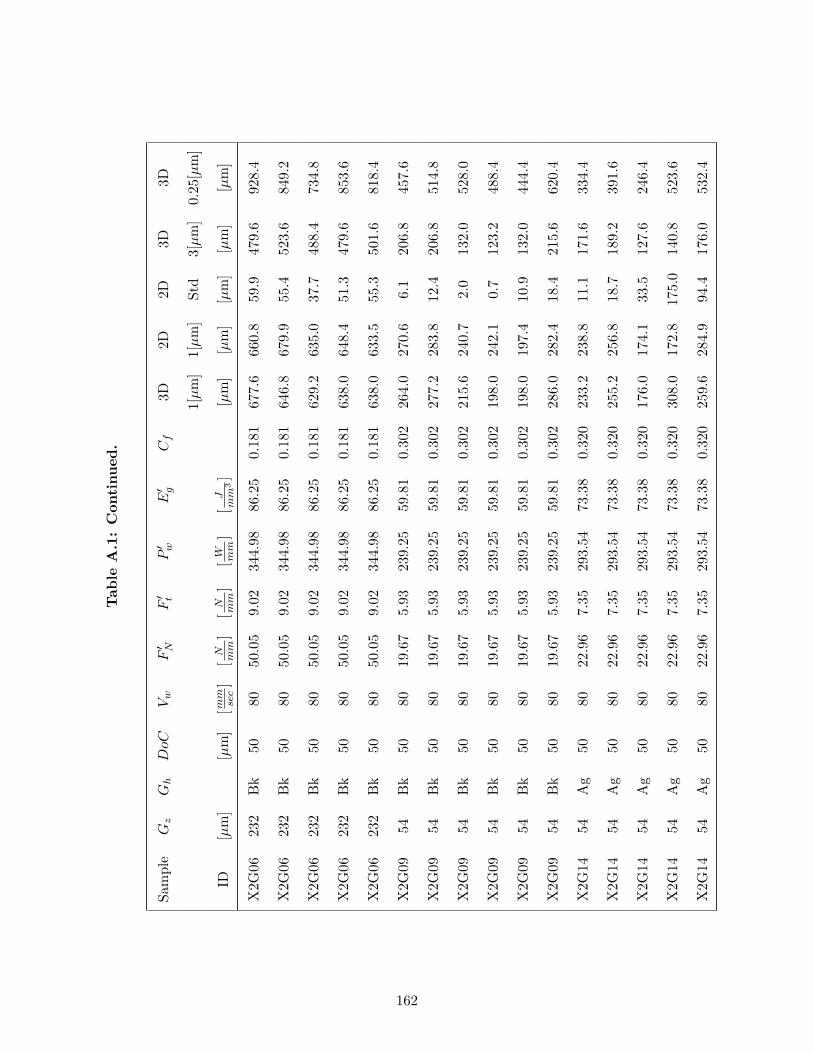
Tab
leA
.1:
Con
tinued
.
Sam
ple
Gz
Gh
DoC
Vw
F′ N
F′ t
P′ w
E′ g
Cf
3D2D
2D3D
3D
1[µm
]1[
µm
]St
d3[
µm
]0.
25[µ
m]
ID[µ
m]
[µm
][m
mse
c]
[N mm
][
N mm
][
W mm
][
Jm
m3]
[µm
][µ
m]
[µm
][µ
m]
[µm
]
X2G
0623
2B
k50
8050
.05
9.02
344.
9886
.25
0.18
167
7.6
660.
859
.947
9.6
928.
4
X2G
0623
2B
k50
8050
.05
9.02
344.
9886
.25
0.18
164
6.8
679.
955
.452
3.6
849.
2
X2G
0623
2B
k50
8050
.05
9.02
344.
9886
.25
0.18
162
9.2
635.
037
.748
8.4
734.
8
X2G
0623
2B
k50
8050
.05
9.02
344.
9886
.25
0.18
163
8.0
648.
451
.347
9.6
853.
6
X2G
0623
2B
k50
8050
.05
9.02
344.
9886
.25
0.18
163
8.0
633.
555
.350
1.6
818.
4
X2G
0954
Bk
5080
19.6
75.
9323
9.25
59.8
10.
302
264.
027
0.6
6.1
206.
845
7.6
X2G
0954
Bk
5080
19.6
75.
9323
9.25
59.8
10.
302
277.
228
3.8
12.4
206.
851
4.8
X2G
0954
Bk
5080
19.6
75.
9323
9.25
59.8
10.
302
215.
624
0.7
2.0
132.
052
8.0
X2G
0954
Bk
5080
19.6
75.
9323
9.25
59.8
10.
302
198.
024
2.1
0.7
123.
248
8.4
X2G
0954
Bk
5080
19.6
75.
9323
9.25
59.8
10.
302
198.
019
7.4
10.9
132.
044
4.4
X2G
0954
Bk
5080
19.6
75.
9323
9.25
59.8
10.
302
286.
028
2.4
18.4
215.
662
0.4
X2G
1454
Ag
5080
22.9
67.
3529
3.54
73.3
80.
320
233.
223
8.8
11.1
171.
633
4.4
X2G
1454
Ag
5080
22.9
67.
3529
3.54
73.3
80.
320
255.
225
6.8
18.7
189.
239
1.6
X2G
1454
Ag
5080
22.9
67.
3529
3.54
73.3
80.
320
176.
017
4.1
33.5
127.
624
6.4
X2G
1454
Ag
5080
22.9
67.
3529
3.54
73.3
80.
320
308.
017
2.8
175.
014
0.8
523.
6
X2G
1454
Ag
5080
22.9
67.
3529
3.54
73.3
80.
320
259.
628
4.9
94.4
176.
053
2.4
162
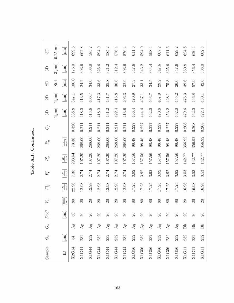
Tab
leA
.1:
Con
tinued
.
Sam
ple
Gz
Gh
DoC
Vw
F′ N
F′ t
P′ w
E′ g
Cf
3D2D
2D3D
3D
1[µm
]1[
µm
]St
d3[
µm
]0.
25[µ
m]
ID[µ
m]
[µm
][m
mse
c]
[N mm
][
N mm
][
W mm
][
Jm
m3]
[µm
][µ
m]
[µm
][µ
m]
[µm
]
X2G
1454
Ag
5080
22.9
67.
3529
3.54
73.3
80.
320
338.
834
7.1
180.
017
6.0
699.
6
X1G
4423
2A
g20
2012
.98
2.74
107.
2026
8.00
0.21
141
8.0
413.
524
.230
3.6
602.
8
X1G
4423
2A
g20
2012
.98
2.74
107.
2026
8.00
0.21
141
3.6
406.
734
.030
8.0
585.
2
X1G
4423
2A
g20
2012
.98
2.74
107.
2026
8.00
0.21
141
8.0
417.
333
.632
5.6
594.
0
X1G
4423
2A
g20
2012
.98
2.74
107.
2026
8.00
0.21
143
1.2
431.
725
.832
1.2
585.
2
X1G
4423
2A
g20
2012
.98
2.74
107.
2026
8.00
0.21
142
2.4
416.
830
.631
2.4
576.
4
X1G
4423
2A
g20
2012
.98
2.74
107.
2026
8.00
0.21
141
3.6
406.
332
.930
3.6
576.
4
X1G
5623
2A
g20
8017
.25
3.92
157.
5698
.48
0.22
746
6.4
470.
927
.334
7.6
611.
6
X1G
5623
2A
g20
8017
.25
3.92
157.
5698
.48
0.22
744
4.4
437.
133
.134
3.2
594.
0
X1G
5623
2A
g20
8017
.25
3.92
157.
5698
.48
0.22
746
2.0
463.
734
.533
4.4
598.
4
X1G
5623
2A
g20
8017
.25
3.92
157.
5698
.48
0.22
747
0.8
467.
929
.234
7.6
607.
2
X1G
5623
2A
g20
8017
.25
3.92
157.
5698
.48
0.22
745
3.2
428.
175
.332
5.6
611.
6
X1G
5623
2A
g20
8017
.25
3.92
157.
5698
.48
0.22
746
2.0
455.
226
.034
7.6
629.
2
X1G
1123
2B
k20
2016
.98
3.53
142.
7735
6.92
0.20
847
9.6
476.
339
.636
0.8
624.
8
X1G
1123
2B
k20
2016
.98
3.53
142.
7735
6.92
0.20
846
2.0
446.
857
.935
6.4
620.
4
X1G
1123
2B
k20
2016
.98
3.53
142.
7735
6.92
0.20
842
2.4
430.
142
.630
8.0
602.
8
163
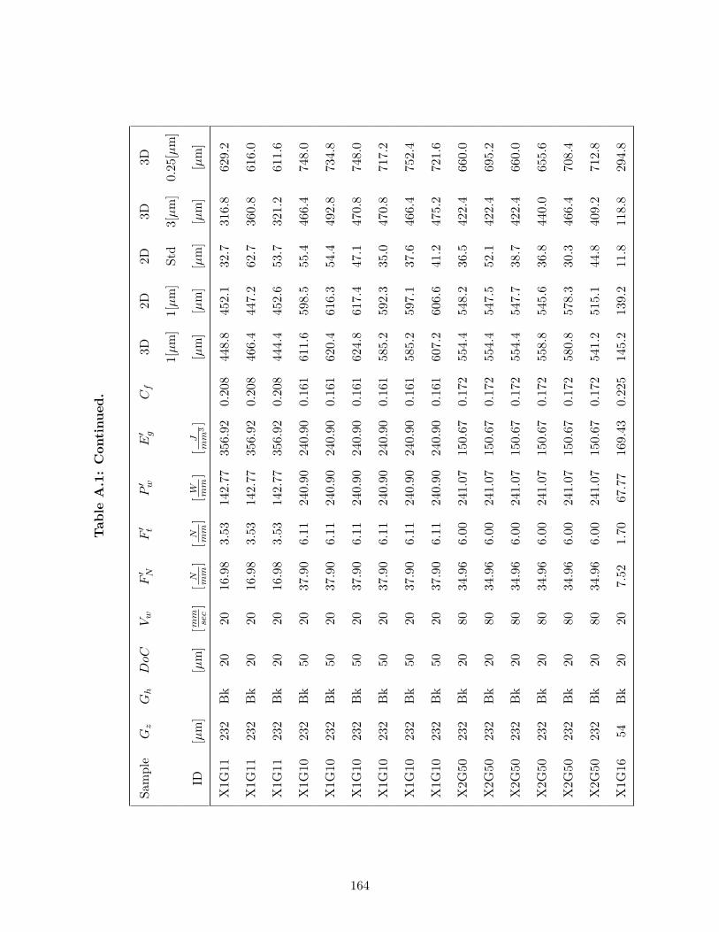
Tab
leA
.1:
Con
tinued
.
Sam
ple
Gz
Gh
DoC
Vw
F′ N
F′ t
P′ w
E′ g
Cf
3D2D
2D3D
3D
1[µm
]1[
µm
]St
d3[
µm
]0.
25[µ
m]
ID[µ
m]
[µm
][m
mse
c]
[N mm
][
N mm
][
W mm
][
Jm
m3]
[µm
][µ
m]
[µm
][µ
m]
[µm
]
X1G
1123
2B
k20
2016
.98
3.53
142.
7735
6.92
0.20
844
8.8
452.
132
.731
6.8
629.
2
X1G
1123
2B
k20
2016
.98
3.53
142.
7735
6.92
0.20
846
6.4
447.
262
.736
0.8
616.
0
X1G
1123
2B
k20
2016
.98
3.53
142.
7735
6.92
0.20
844
4.4
452.
653
.732
1.2
611.
6
X1G
1023
2B
k50
2037
.90
6.11
240.
9024
0.90
0.16
161
1.6
598.
555
.446
6.4
748.
0
X1G
1023
2B
k50
2037
.90
6.11
240.
9024
0.90
0.16
162
0.4
616.
354
.449
2.8
734.
8
X1G
1023
2B
k50
2037
.90
6.11
240.
9024
0.90
0.16
162
4.8
617.
447
.147
0.8
748.
0
X1G
1023
2B
k50
2037
.90
6.11
240.
9024
0.90
0.16
158
5.2
592.
335
.047
0.8
717.
2
X1G
1023
2B
k50
2037
.90
6.11
240.
9024
0.90
0.16
158
5.2
597.
137
.646
6.4
752.
4
X1G
1023
2B
k50
2037
.90
6.11
240.
9024
0.90
0.16
160
7.2
606.
641
.247
5.2
721.
6
X2G
5023
2B
k20
8034
.96
6.00
241.
0715
0.67
0.17
255
4.4
548.
236
.542
2.4
660.
0
X2G
5023
2B
k20
8034
.96
6.00
241.
0715
0.67
0.17
255
4.4
547.
552
.142
2.4
695.
2
X2G
5023
2B
k20
8034
.96
6.00
241.
0715
0.67
0.17
255
4.4
547.
738
.742
2.4
660.
0
X2G
5023
2B
k20
8034
.96
6.00
241.
0715
0.67
0.17
255
8.8
545.
636
.844
0.0
655.
6
X2G
5023
2B
k20
8034
.96
6.00
241.
0715
0.67
0.17
258
0.8
578.
330
.346
6.4
708.
4
X2G
5023
2B
k20
8034
.96
6.00
241.
0715
0.67
0.17
254
1.2
515.
144
.840
9.2
712.
8
X1G
1654
Bk
2020
7.52
1.70
67.7
716
9.43
0.22
514
5.2
139.
211
.811
8.8
294.
8
164
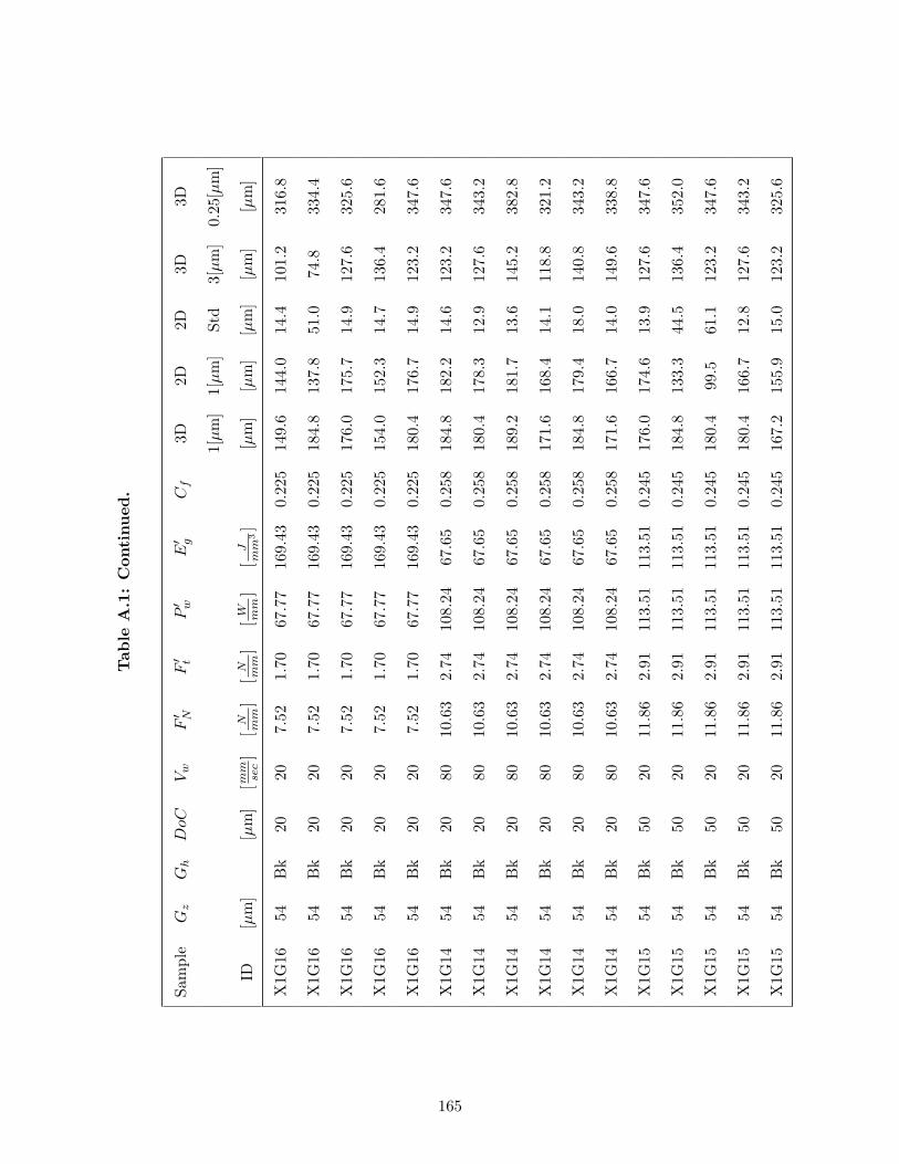
Tab
leA
.1:
Con
tinued
.
Sam
ple
Gz
Gh
DoC
Vw
F′ N
F′ t
P′ w
E′ g
Cf
3D2D
2D3D
3D
1[µm
]1[
µm
]St
d3[
µm
]0.
25[µ
m]
ID[µ
m]
[µm
][m
mse
c]
[N mm
][
N mm
][
W mm
][
Jm
m3]
[µm
][µ
m]
[µm
][µ
m]
[µm
]
X1G
1654
Bk
2020
7.52
1.70
67.7
716
9.43
0.22
514
9.6
144.
014
.410
1.2
316.
8
X1G
1654
Bk
2020
7.52
1.70
67.7
716
9.43
0.22
518
4.8
137.
851
.074
.833
4.4
X1G
1654
Bk
2020
7.52
1.70
67.7
716
9.43
0.22
517
6.0
175.
714
.912
7.6
325.
6
X1G
1654
Bk
2020
7.52
1.70
67.7
716
9.43
0.22
515
4.0
152.
314
.713
6.4
281.
6
X1G
1654
Bk
2020
7.52
1.70
67.7
716
9.43
0.22
518
0.4
176.
714
.912
3.2
347.
6
X1G
1454
Bk
2080
10.6
32.
7410
8.24
67.6
50.
258
184.
818
2.2
14.6
123.
234
7.6
X1G
1454
Bk
2080
10.6
32.
7410
8.24
67.6
50.
258
180.
417
8.3
12.9
127.
634
3.2
X1G
1454
Bk
2080
10.6
32.
7410
8.24
67.6
50.
258
189.
218
1.7
13.6
145.
238
2.8
X1G
1454
Bk
2080
10.6
32.
7410
8.24
67.6
50.
258
171.
616
8.4
14.1
118.
832
1.2
X1G
1454
Bk
2080
10.6
32.
7410
8.24
67.6
50.
258
184.
817
9.4
18.0
140.
834
3.2
X1G
1454
Bk
2080
10.6
32.
7410
8.24
67.6
50.
258
171.
616
6.7
14.0
149.
633
8.8
X1G
1554
Bk
5020
11.8
62.
9111
3.51
113.
510.
245
176.
017
4.6
13.9
127.
634
7.6
X1G
1554
Bk
5020
11.8
62.
9111
3.51
113.
510.
245
184.
813
3.3
44.5
136.
435
2.0
X1G
1554
Bk
5020
11.8
62.
9111
3.51
113.
510.
245
180.
499
.561
.112
3.2
347.
6
X1G
1554
Bk
5020
11.8
62.
9111
3.51
113.
510.
245
180.
416
6.7
12.8
127.
634
3.2
X1G
1554
Bk
5020
11.8
62.
9111
3.51
113.
510.
245
167.
215
5.9
15.0
123.
232
5.6
165
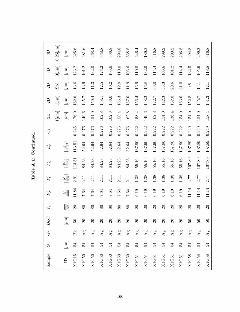
Tab
leA
.1:
Con
tinued
.
Sam
ple
Gz
Gh
DoC
Vw
F′ N
F′ t
P′ w
E′ g
Cf
3D2D
2D3D
3D
1[µm
]1[
µm
]St
d3[
µm
]0.
25[µ
m]
ID[µ
m]
[µm
][m
mse
c]
[N mm
][
N mm
][
W mm
][
Jm
m3]
[µm
][µ
m]
[µm
][µ
m]
[µm
]
X1G
1554
Bk
5020
11.8
62.
9111
3.51
113.
510.
245
176.
016
2.6
13.6
123.
232
5.6
X1G
5054
Ag
2080
7.64
2.11
84.2
352
.64
0.27
614
9.6
145.
713
.910
1.2
281.
6
X1G
5054
Ag
2080
7.64
2.11
84.2
352
.64
0.27
615
4.0
150.
411
.313
2.0
268.
4
X1G
5054
Ag
2080
7.64
2.11
84.2
352
.64
0.27
616
2.8
158.
112
.512
3.2
338.
8
X1G
5054
Ag
2080
7.64
2.11
84.2
352
.64
0.27
616
2.8
158.
010
.210
5.6
338.
8
X1G
5054
Ag
2080
7.64
2.11
84.2
352
.64
0.27
615
8.4
156.
312
.911
0.0
294.
8
X1G
5054
Ag
2080
7.64
2.11
84.2
352
.64
0.27
616
2.8
157.
011
.910
5.6
338.
8
X1G
5154
Ag
2020
6.19
1.38
55.1
613
7.90
0.22
215
8.4
156.
416
.911
0.0
246.
4
X1G
5154
Ag
2020
6.19
1.38
55.1
613
7.90
0.22
214
9.6
148.
216
.813
2.0
189.
2
X1G
5154
Ag
2020
6.19
1.38
55.1
613
7.90
0.22
216
2.8
122.
736
.011
4.4
316.
8
X1G
5154
Ag
2020
6.19
1.38
55.1
613
7.90
0.22
215
4.0
142.
335
.310
5.6
299.
2
X1G
5154
Ag
2020
6.19
1.38
55.1
613
7.90
0.22
213
6.4
132.
820
.610
1.2
299.
2
X1G
5154
Ag
2020
6.19
1.38
55.1
613
7.90
0.22
215
4.0
163.
031
.011
4.4
206.
8
X1G
5854
Ag
5020
11.1
42.
7710
7.89
107.
890.
249
154.
015
2.8
9.8
132.
029
4.8
X1G
5854
Ag
5020
11.1
42.
7710
7.89
107.
890.
249
154.
014
5.7
14.1
105.
629
9.2
X1G
5854
Ag
5020
11.1
42.
7710
7.89
107.
890.
249
158.
415
1.3
12.1
118.
831
6.8
166
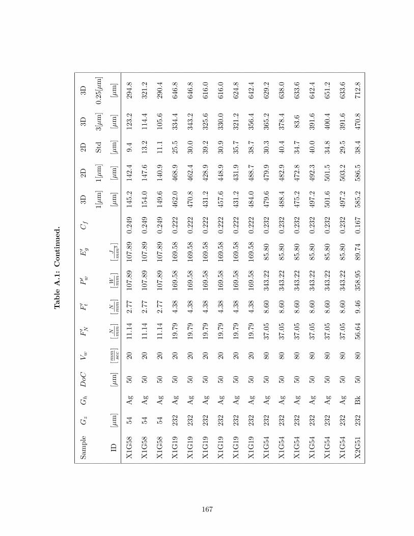
Tab
leA
.1:
Con
tinued
.
Sam
ple
Gz
Gh
DoC
Vw
F′ N
F′ t
P′ w
E′ g
Cf
3D2D
2D3D
3D
1[µm
]1[
µm
]St
d3[
µm
]0.
25[µ
m]
ID[µ
m]
[µm
][m
mse
c]
[N mm
][
N mm
][
W mm
][
Jm
m3]
[µm
][µ
m]
[µm
][µ
m]
[µm
]
X1G
5854
Ag
5020
11.1
42.
7710
7.89
107.
890.
249
145.
214
2.4
9.4
123.
229
4.8
X1G
5854
Ag
5020
11.1
42.
7710
7.89
107.
890.
249
154.
014
7.6
13.2
114.
432
1.2
X1G
5854
Ag
5020
11.1
42.
7710
7.89
107.
890.
249
149.
614
0.9
11.1
105.
629
0.4
X1G
1923
2A
g50
2019
.79
4.38
169.
5816
9.58
0.22
246
2.0
468.
925
.533
4.4
646.
8
X1G
1923
2A
g50
2019
.79
4.38
169.
5816
9.58
0.22
247
0.8
462.
430
.034
3.2
646.
8
X1G
1923
2A
g50
2019
.79
4.38
169.
5816
9.58
0.22
243
1.2
428.
939
.232
5.6
616.
0
X1G
1923
2A
g50
2019
.79
4.38
169.
5816
9.58
0.22
245
7.6
448.
930
.933
0.0
616.
0
X1G
1923
2A
g50
2019
.79
4.38
169.
5816
9.58
0.22
243
1.2
431.
935
.732
1.2
624.
8
X1G
1923
2A
g50
2019
.79
4.38
169.
5816
9.58
0.22
248
4.0
488.
738
.735
6.4
642.
4
X1G
5423
2A
g50
8037
.05
8.60
343.
2285
.80
0.23
247
9.6
479.
930
.336
5.2
629.
2
X1G
5423
2A
g50
8037
.05
8.60
343.
2285
.80
0.23
248
8.4
482.
940
.437
8.4
638.
0
X1G
5423
2A
g50
8037
.05
8.60
343.
2285
.80
0.23
247
5.2
472.
834
.783
.663
3.6
X1G
5423
2A
g50
8037
.05
8.60
343.
2285
.80
0.23
249
7.2
492.
340
.039
1.6
642.
4
X1G
5423
2A
g50
8037
.05
8.60
343.
2285
.80
0.23
250
1.6
501.
534
.840
0.4
651.
2
X1G
5423
2A
g50
8037
.05
8.60
343.
2285
.80
0.23
249
7.2
503.
229
.539
1.6
633.
6
X2G
5123
2B
k50
8056
.64
9.46
358.
9589
.74
0.16
758
5.2
586.
538
.447
0.8
712.
8
167
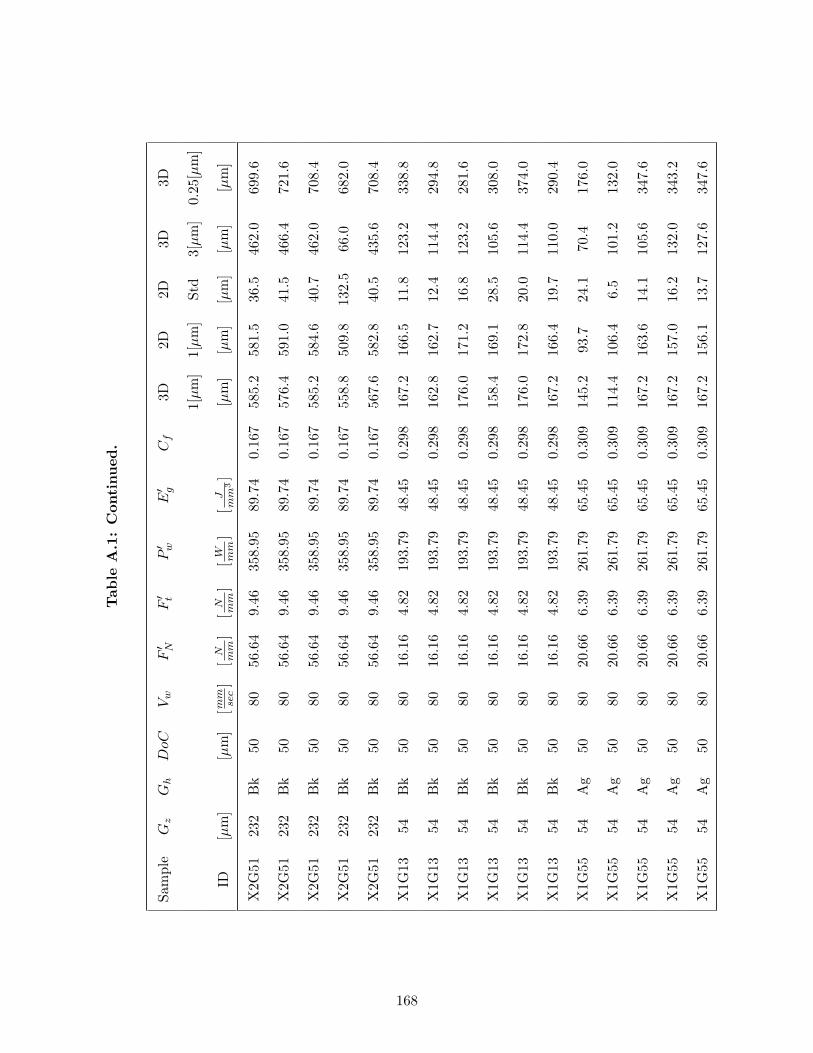
Tab
leA
.1:
Con
tinued
.
Sam
ple
Gz
Gh
DoC
Vw
F′ N
F′ t
P′ w
E′ g
Cf
3D2D
2D3D
3D
1[µm
]1[
µm
]St
d3[
µm
]0.
25[µ
m]
ID[µ
m]
[µm
][m
mse
c]
[N mm
][
N mm
][
W mm
][
Jm
m3]
[µm
][µ
m]
[µm
][µ
m]
[µm
]
X2G
5123
2B
k50
8056
.64
9.46
358.
9589
.74
0.16
758
5.2
581.
536
.546
2.0
699.
6
X2G
5123
2B
k50
8056
.64
9.46
358.
9589
.74
0.16
757
6.4
591.
041
.546
6.4
721.
6
X2G
5123
2B
k50
8056
.64
9.46
358.
9589
.74
0.16
758
5.2
584.
640
.746
2.0
708.
4
X2G
5123
2B
k50
8056
.64
9.46
358.
9589
.74
0.16
755
8.8
509.
813
2.5
66.0
682.
0
X2G
5123
2B
k50
8056
.64
9.46
358.
9589
.74
0.16
756
7.6
582.
840
.543
5.6
708.
4
X1G
1354
Bk
5080
16.1
64.
8219
3.79
48.4
50.
298
167.
216
6.5
11.8
123.
233
8.8
X1G
1354
Bk
5080
16.1
64.
8219
3.79
48.4
50.
298
162.
816
2.7
12.4
114.
429
4.8
X1G
1354
Bk
5080
16.1
64.
8219
3.79
48.4
50.
298
176.
017
1.2
16.8
123.
228
1.6
X1G
1354
Bk
5080
16.1
64.
8219
3.79
48.4
50.
298
158.
416
9.1
28.5
105.
630
8.0
X1G
1354
Bk
5080
16.1
64.
8219
3.79
48.4
50.
298
176.
017
2.8
20.0
114.
437
4.0
X1G
1354
Bk
5080
16.1
64.
8219
3.79
48.4
50.
298
167.
216
6.4
19.7
110.
029
0.4
X1G
5554
Ag
5080
20.6
66.
3926
1.79
65.4
50.
309
145.
293
.724
.170
.417
6.0
X1G
5554
Ag
5080
20.6
66.
3926
1.79
65.4
50.
309
114.
410
6.4
6.5
101.
213
2.0
X1G
5554
Ag
5080
20.6
66.
3926
1.79
65.4
50.
309
167.
216
3.6
14.1
105.
634
7.6
X1G
5554
Ag
5080
20.6
66.
3926
1.79
65.4
50.
309
167.
215
7.0
16.2
132.
034
3.2
X1G
5554
Ag
5080
20.6
66.
3926
1.79
65.4
50.
309
167.
215
6.1
13.7
127.
634
7.6
168
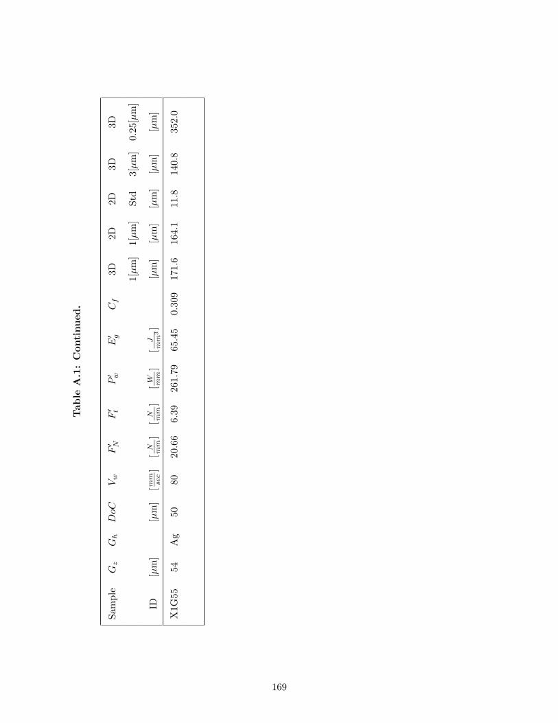
Tab
leA
.1:
Con
tinued
.
Sam
ple
Gz
Gh
DoC
Vw
F′ N
F′ t
P′ w
E′ g
Cf
3D2D
2D3D
3D
1[µm
]1[
µm
]St
d3[
µm
]0.
25[µ
m]
ID[µ
m]
[µm
][m
mse
c]
[N mm
][
N mm
][
W mm
][
Jm
m3]
[µm
][µ
m]
[µm
][µ
m]
[µm
]
X1G
5554
Ag
5080
20.6
66.
3926
1.79
65.4
50.
309
171.
616
4.1
11.8
140.
835
2.0
169
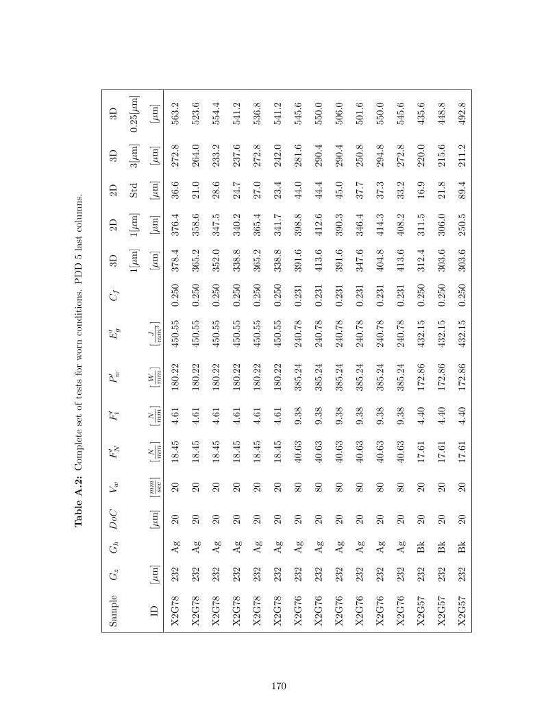
Tab
leA
.2:
Com
plet
ese
tof
test
sfo
rw
orn
cond
itio
ns.
PD
D5
last
colu
mns
.
Sam
ple
Gz
Gh
DoC
Vw
F′ N
F′ t
P′ w
E′ g
Cf
3D2D
2D3D
3D
1[µm
]1[
µm
]St
d3[
µm
]0.
25[µ
m]
ID[µ
m]
[µm
][m
mse
c]
[N mm
][
N mm
][
W mm
][
Jm
m3]
[µm
][µ
m]
[µm
][µ
m]
[µm
]
X2G
7823
2A
g20
2018
.45
4.61
180.
2245
0.55
0.25
037
8.4
376.
436
.627
2.8
563.
2
X2G
7823
2A
g20
2018
.45
4.61
180.
2245
0.55
0.25
036
5.2
358.
621
.026
4.0
523.
6
X2G
7823
2A
g20
2018
.45
4.61
180.
2245
0.55
0.25
035
2.0
347.
528
.623
3.2
554.
4
X2G
7823
2A
g20
2018
.45
4.61
180.
2245
0.55
0.25
033
8.8
340.
224
.723
7.6
541.
2
X2G
7823
2A
g20
2018
.45
4.61
180.
2245
0.55
0.25
036
5.2
365.
427
.027
2.8
536.
8
X2G
7823
2A
g20
2018
.45
4.61
180.
2245
0.55
0.25
033
8.8
341.
723
.424
2.0
541.
2
X2G
7623
2A
g20
8040
.63
9.38
385.
2424
0.78
0.23
139
1.6
398.
844
.028
1.6
545.
6
X2G
7623
2A
g20
8040
.63
9.38
385.
2424
0.78
0.23
141
3.6
412.
644
.429
0.4
550.
0
X2G
7623
2A
g20
8040
.63
9.38
385.
2424
0.78
0.23
139
1.6
390.
345
.029
0.4
506.
0
X2G
7623
2A
g20
8040
.63
9.38
385.
2424
0.78
0.23
134
7.6
346.
437
.725
0.8
501.
6
X2G
7623
2A
g20
8040
.63
9.38
385.
2424
0.78
0.23
140
4.8
414.
337
.329
4.8
550.
0
X2G
7623
2A
g20
8040
.63
9.38
385.
2424
0.78
0.23
141
3.6
408.
233
.227
2.8
545.
6
X2G
5723
2B
k20
2017
.61
4.40
172.
8643
2.15
0.25
031
2.4
311.
516
.922
0.0
435.
6
X2G
5723
2B
k20
2017
.61
4.40
172.
8643
2.15
0.25
030
3.6
306.
021
.821
5.6
448.
8
X2G
5723
2B
k20
2017
.61
4.40
172.
8643
2.15
0.25
030
3.6
250.
589
.421
1.2
492.
8
170
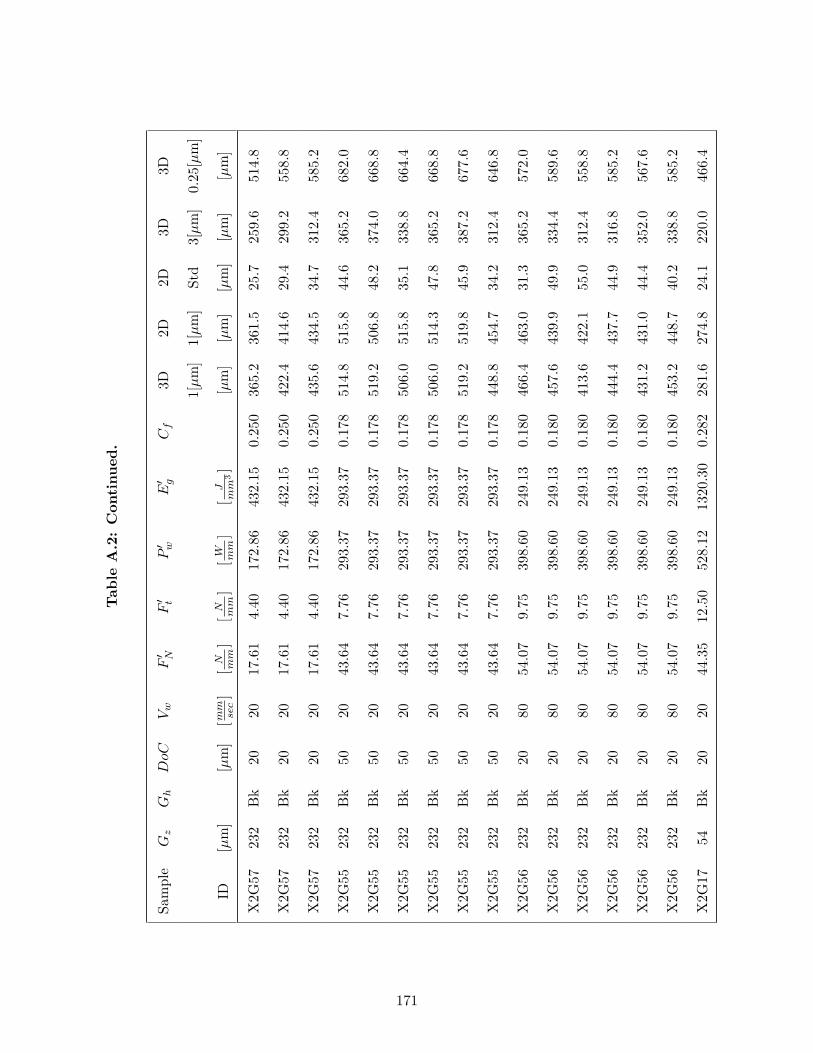
Tab
leA
.2:
Con
tinued
.
Sam
ple
Gz
Gh
DoC
Vw
F′ N
F′ t
P′ w
E′ g
Cf
3D2D
2D3D
3D
1[µm
]1[
µm
]St
d3[
µm
]0.
25[µ
m]
ID[µ
m]
[µm
][m
mse
c]
[N mm
][
N mm
][
W mm
][
Jm
m3]
[µm
][µ
m]
[µm
][µ
m]
[µm
]
X2G
5723
2B
k20
2017
.61
4.40
172.
8643
2.15
0.25
036
5.2
361.
525
.725
9.6
514.
8
X2G
5723
2B
k20
2017
.61
4.40
172.
8643
2.15
0.25
042
2.4
414.
629
.429
9.2
558.
8
X2G
5723
2B
k20
2017
.61
4.40
172.
8643
2.15
0.25
043
5.6
434.
534
.731
2.4
585.
2
X2G
5523
2B
k50
2043
.64
7.76
293.
3729
3.37
0.17
851
4.8
515.
844
.636
5.2
682.
0
X2G
5523
2B
k50
2043
.64
7.76
293.
3729
3.37
0.17
851
9.2
506.
848
.237
4.0
668.
8
X2G
5523
2B
k50
2043
.64
7.76
293.
3729
3.37
0.17
850
6.0
515.
835
.133
8.8
664.
4
X2G
5523
2B
k50
2043
.64
7.76
293.
3729
3.37
0.17
850
6.0
514.
347
.836
5.2
668.
8
X2G
5523
2B
k50
2043
.64
7.76
293.
3729
3.37
0.17
851
9.2
519.
845
.938
7.2
677.
6
X2G
5523
2B
k50
2043
.64
7.76
293.
3729
3.37
0.17
844
8.8
454.
734
.231
2.4
646.
8
X2G
5623
2B
k20
8054
.07
9.75
398.
6024
9.13
0.18
046
6.4
463.
031
.336
5.2
572.
0
X2G
5623
2B
k20
8054
.07
9.75
398.
6024
9.13
0.18
045
7.6
439.
949
.933
4.4
589.
6
X2G
5623
2B
k20
8054
.07
9.75
398.
6024
9.13
0.18
041
3.6
422.
155
.031
2.4
558.
8
X2G
5623
2B
k20
8054
.07
9.75
398.
6024
9.13
0.18
044
4.4
437.
744
.931
6.8
585.
2
X2G
5623
2B
k20
8054
.07
9.75
398.
6024
9.13
0.18
043
1.2
431.
044
.435
2.0
567.
6
X2G
5623
2B
k20
8054
.07
9.75
398.
6024
9.13
0.18
045
3.2
448.
740
.233
8.8
585.
2
X2G
1754
Bk
2020
44.3
512
.50
528.
1213
20.3
00.
282
281.
627
4.8
24.1
220.
046
6.4
171
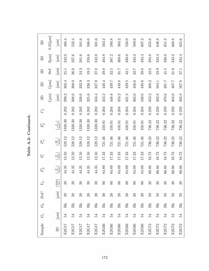
Tab
leA
.2:
Con
tinued
.
Sam
ple
Gz
Gh
DoC
Vw
F′ N
F′ t
P′ w
E′ g
Cf
3D2D
2D3D
3D
1[µm
]1[
µm
]St
d3[
µm
]0.
25[µ
m]
ID[µ
m]
[µm
][m
mse
c]
[N mm
][
N mm
][
W mm
][
Jm
m3]
[µm
][µ
m]
[µm
][µ
m]
[µm
]
X2G
1754
Bk
2020
44.3
512
.50
528.
1213
20.3
00.
282
299.
230
2.4
25.1
242.
046
6.4
X2G
1754
Bk
2020
44.3
512
.50
528.
1213
20.3
00.
282
308.
030
8.0
26.0
237.
653
2.4
X2G
1754
Bk
2020
44.3
512
.50
528.
1213
20.3
00.
282
330.
033
2.9
24.3
281.
650
1.6
X2G
1754
Bk
2020
44.3
512
.50
528.
1213
20.3
00.
282
325.
632
6.3
19.3
259.
650
6.0
X2G
1754
Bk
2020
44.3
512
.50
528.
1213
20.3
00.
282
334.
432
7.9
27.0
242.
050
1.6
X2G
6654
Bk
2080
84.8
917
.33
721.
4645
0.91
0.20
445
3.2
440.
429
.840
4.8
563.
2
X2G
6654
Bk
2080
84.8
917
.33
721.
4645
0.91
0.20
444
8.8
439.
732
.538
7.2
580.
8
X2G
6654
Bk
2080
84.8
917
.33
721.
4645
0.91
0.20
445
3.2
449.
831
.736
9.6
563.
2
X2G
6654
Bk
2080
84.8
917
.33
721.
4645
0.91
0.20
443
1.2
429.
542
.133
0.0
550.
0
X2G
6654
Bk
2080
84.8
917
.33
721.
4645
0.91
0.20
446
2.0
456.
632
.734
3.2
589.
6
X2G
6654
Bk
2080
84.8
917
.33
721.
4645
0.91
0.20
444
0.0
438.
629
.033
4.4
607.
2
X2G
7254
Bk
5020
66.8
616
.73
736.
2273
6.22
0.25
045
3.2
468.
242
.029
4.8
655.
6
X2G
7254
Bk
5020
66.8
616
.73
736.
2273
6.22
0.25
049
2.8
504.
133
.933
4.4
646.
8
X2G
7254
Bk
5020
66.8
616
.73
736.
2273
6.22
0.25
047
9.6
491.
741
.533
0.0
651.
2
X2G
7254
Bk
5020
66.8
616
.73
736.
2273
6.22
0.25
048
4.0
487.
731
.834
3.2
668.
8
X2G
7254
Bk
5020
66.8
616
.73
736.
2273
6.22
0.25
049
2.8
507.
837
.133
4.4
655.
6
172
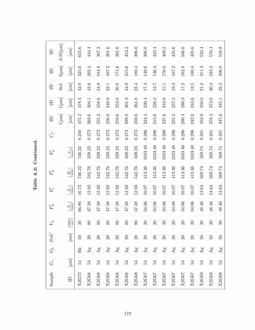
Tab
leA
.2:
Con
tinued
.
Sam
ple
Gz
Gh
DoC
Vw
F′ N
F′ t
P′ w
E′ g
Cf
3D2D
2D3D
3D
1[µm
]1[
µm
]St
d3[
µm
]0.
25[µ
m]
ID[µ
m]
[µm
][m
mse
c]
[N mm
][
N mm
][
W mm
][
Jm
m3]
[µm
][µ
m]
[µm
][µ
m]
[µm
]
X2G
7254
Bk
5020
66.8
616
.73
736.
2273
6.22
0.25
047
5.2
478.
442
.032
5.6
655.
6
X2G
6854
Ag
2080
47.3
812
.93
542.
7633
9.23
0.27
330
3.6
304.
143
.820
2.4
444.
4
X2G
6854
Ag
2080
47.3
812
.93
542.
7633
9.23
0.27
325
5.2
258.
624
.918
4.8
387.
2
X2G
6854
Ag
2080
47.3
812
.93
542.
7633
9.23
0.27
325
0.8
248.
923
.116
7.2
391.
6
X2G
6854
Ag
2080
47.3
812
.93
542.
7633
9.23
0.27
325
9.6
253.
820
.817
1.6
391.
6
X2G
6854
Ag
2080
47.3
812
.93
542.
7633
9.23
0.27
329
9.2
301.
334
.921
5.6
453.
2
X2G
6854
Ag
2080
47.3
812
.93
542.
7633
9.23
0.27
325
9.6
261.
823
.418
0.4
396.
0
X2G
6754
Ag
2020
34.0
610
.07
413.
3610
33.4
00.
296
224.
423
9.4
17.4
149.
639
6.0
X2G
6754
Ag
2020
34.0
610
.07
413.
3610
33.4
00.
296
215.
622
6.2
12.7
136.
442
2.4
X2G
6754
Ag
2020
34.0
610
.07
413.
3610
33.4
00.
296
237.
624
3.8
15.1
176.
040
9.2
X2G
6754
Ag
2020
34.0
610
.07
413.
3610
33.4
00.
296
255.
225
7.5
19.3
167.
243
5.6
X2G
6754
Ag
2020
34.0
610
.07
413.
3610
33.4
00.
296
290.
428
6.3
17.2
162.
850
6.0
X2G
6754
Ag
2020
34.0
610
.07
413.
3610
33.4
00.
296
242.
024
3.6
13.5
180.
443
5.6
X2G
6954
Ag
5020
48.4
613
.64
569.
7456
9.74
0.28
135
2.0
350.
021
.221
1.2
532.
4
X2G
6954
Ag
5020
48.4
613
.64
569.
7456
9.74
0.28
137
8.4
373.
030
.323
3.2
576.
4
X2G
6954
Ag
5020
48.4
613
.64
569.
7456
9.74
0.28
134
7.6
345.
129
.220
6.8
558.
8
173
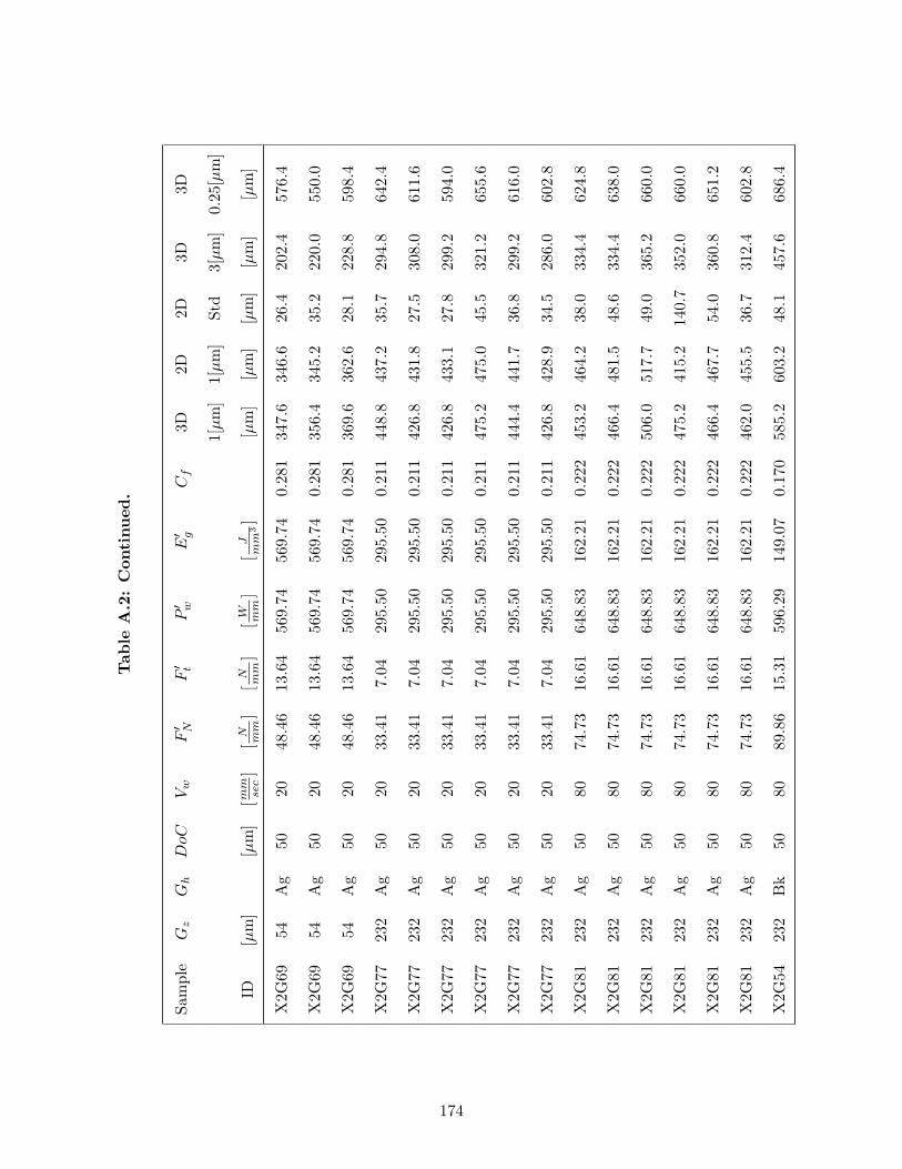
Tab
leA
.2:
Con
tinued
.
Sam
ple
Gz
Gh
DoC
Vw
F′ N
F′ t
P′ w
E′ g
Cf
3D2D
2D3D
3D
1[µm
]1[
µm
]St
d3[
µm
]0.
25[µ
m]
ID[µ
m]
[µm
][m
mse
c]
[N mm
][
N mm
][
W mm
][
Jm
m3]
[µm
][µ
m]
[µm
][µ
m]
[µm
]
X2G
6954
Ag
5020
48.4
613
.64
569.
7456
9.74
0.28
134
7.6
346.
626
.420
2.4
576.
4
X2G
6954
Ag
5020
48.4
613
.64
569.
7456
9.74
0.28
135
6.4
345.
235
.222
0.0
550.
0
X2G
6954
Ag
5020
48.4
613
.64
569.
7456
9.74
0.28
136
9.6
362.
628
.122
8.8
598.
4
X2G
7723
2A
g50
2033
.41
7.04
295.
5029
5.50
0.21
144
8.8
437.
235
.729
4.8
642.
4
X2G
7723
2A
g50
2033
.41
7.04
295.
5029
5.50
0.21
142
6.8
431.
827
.530
8.0
611.
6
X2G
7723
2A
g50
2033
.41
7.04
295.
5029
5.50
0.21
142
6.8
433.
127
.829
9.2
594.
0
X2G
7723
2A
g50
2033
.41
7.04
295.
5029
5.50
0.21
147
5.2
475.
045
.532
1.2
655.
6
X2G
7723
2A
g50
2033
.41
7.04
295.
5029
5.50
0.21
144
4.4
441.
736
.829
9.2
616.
0
X2G
7723
2A
g50
2033
.41
7.04
295.
5029
5.50
0.21
142
6.8
428.
934
.528
6.0
602.
8
X2G
8123
2A
g50
8074
.73
16.6
164
8.83
162.
210.
222
453.
246
4.2
38.0
334.
462
4.8
X2G
8123
2A
g50
8074
.73
16.6
164
8.83
162.
210.
222
466.
448
1.5
48.6
334.
463
8.0
X2G
8123
2A
g50
8074
.73
16.6
164
8.83
162.
210.
222
506.
051
7.7
49.0
365.
266
0.0
X2G
8123
2A
g50
8074
.73
16.6
164
8.83
162.
210.
222
475.
241
5.2
140.
735
2.0
660.
0
X2G
8123
2A
g50
8074
.73
16.6
164
8.83
162.
210.
222
466.
446
7.7
54.0
360.
865
1.2
X2G
8123
2A
g50
8074
.73
16.6
164
8.83
162.
210.
222
462.
045
5.5
36.7
312.
460
2.8
X2G
5423
2B
k50
8089
.86
15.3
159
6.29
149.
070.
170
585.
260
3.2
48.1
457.
668
6.4
174
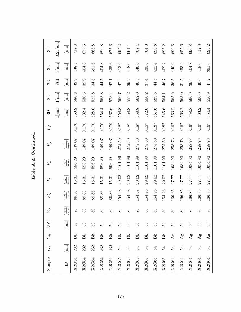
Tab
leA
.2:
Con
tinued
.
Sam
ple
Gz
Gh
DoC
Vw
F′ N
F′ t
P′ w
E′ g
Cf
3D2D
2D3D
3D
1[µm
]1[
µm
]St
d3[
µm
]0.
25[µ
m]
ID[µ
m]
[µm
][m
mse
c]
[N mm
][
N mm
][
W mm
][
Jm
m3]
[µm
][µ
m]
[µm
][µ
m]
[µm
]
X2G
5423
2B
k50
8089
.86
15.3
159
6.29
149.
070.
170
563.
258
0.8
42.9
448.
871
2.8
X2G
5423
2B
k50
8089
.86
15.3
159
6.29
149.
070.
170
532.
453
0.5
39.9
404.
867
7.6
X2G
5423
2B
k50
8089
.86
15.3
159
6.29
149.
070.
170
528.
052
2.8
34.5
391.
666
8.8
X2G
5423
2B
k50
8089
.86
15.3
159
6.29
149.
070.
170
554.
456
3.8
44.5
404.
869
0.8
X2G
5423
2B
k50
8089
.86
15.3
159
6.29
149.
070.
170
567.
657
8.4
47.1
435.
667
7.6
X2G
6554
Bk
5080
154.
9829
.02
1101
.99
275.
500.
187
558.
856
0.7
47.4
413.
669
5.2
X2G
6554
Bk
5080
154.
9829
.02
1101
.99
275.
500.
187
558.
855
7.2
39.2
418.
066
4.4
X2G
6554
Bk
5080
154.
9829
.02
1101
.99
275.
500.
187
558.
856
2.0
46.3
440.
070
8.4
X2G
6554
Bk
5080
154.
9829
.02
1101
.99
275.
500.
187
572.
058
0.2
37.4
435.
670
4.0
X2G
6554
Bk
5080
154.
9829
.02
1101
.99
275.
500.
187
567.
658
9.5
44.5
422.
469
0.8
X2G
6554
Bk
5080
154.
9829
.02
1101
.99
275.
500.
187
545.
656
4.1
46.7
409.
269
5.2
X2G
6454
Ag
5080
166.
8527
.77
1034
.90
258.
730.
167
563.
256
5.2
36.5
440.
069
9.6
X2G
6454
Ag
5080
166.
8527
.77
1034
.90
258.
730.
167
563.
256
3.0
31.5
453.
265
5.6
X2G
6454
Ag
5080
166.
8527
.77
1034
.90
258.
730.
167
558.
856
0.9
39.5
404.
869
0.8
X2G
6454
Ag
5080
166.
8527
.77
1034
.90
258.
730.
167
563.
256
0.6
46.6
418.
071
2.8
X2G
6454
Ag
5080
166.
8527
.77
1034
.90
258.
730.
167
554.
455
0.9
47.2
391.
669
5.2
175
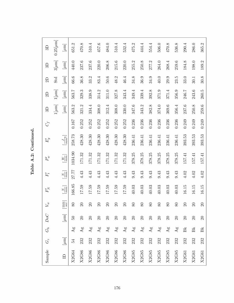
Tab
leA
.2:
Con
tinued
.
Sam
ple
Gz
Gh
DoC
Vw
F′ N
F′ t
P′ w
E′ g
Cf
3D2D
2D3D
3D
1[µm
]1[
µm
]St
d3[
µm
]0.
25[µ
m]
ID[µ
m]
[µm
][m
mse
c]
[N mm
][
N mm
][
W mm
][
Jm
m3]
[µm
][µ
m]
[µm
][µ
m]
[µm
]
X2G
6454
Ag
5080
166.
8527
.77
1034
.90
258.
730.
167
563.
256
3.7
66.6
440.
065
1.2
X2G
8623
2A
g20
2017
.59
4.43
171.
3242
8.30
0.25
232
1.2
329.
336
.823
7.6
470.
8
X2G
8623
2A
g20
2017
.59
4.43
171.
3242
8.30
0.25
233
4.4
338.
933
.223
7.6
510.
4
X2G
8623
2A
g20
2017
.59
4.43
171.
3242
8.30
0.25
230
8.0
314.
283
.422
0.0
457.
6
X2G
8623
2A
g20
2017
.59
4.43
171.
3242
8.30
0.25
231
2.4
311.
050
.620
6.8
484.
0
X2G
8623
2A
g20
2017
.59
4.43
171.
3242
8.30
0.25
230
8.0
327.
848
.221
5.6
510.
4
X2G
8623
2A
g20
2017
.59
4.43
171.
3242
8.30
0.25
233
0.0
343.
446
.422
0.0
532.
4
X2G
8523
2A
g20
8040
.03
9.43
378.
2523
6.41
0.23
634
7.6
349.
434
.825
5.2
475.
2
X2G
8523
2A
g20
8040
.03
9.43
378.
2523
6.41
0.23
634
3.2
339.
436
.925
0.8
444.
4
X2G
8523
2A
g20
8040
.03
9.43
378.
2523
6.41
0.23
638
2.8
392.
834
.927
7.2
554.
4
X2G
8523
2A
g20
8040
.03
9.43
378.
2523
6.41
0.23
637
4.0
371.
940
.026
4.0
506.
0
X2G
8523
2A
g20
8040
.03
9.43
378.
2523
6.41
0.23
636
9.6
371.
429
.926
8.4
470.
8
X2G
8523
2A
g20
8040
.03
9.43
378.
2523
6.41
0.23
635
6.4
356.
923
.525
9.6
536.
8
X2G
6123
2B
k20
2016
.15
4.02
157.
4139
3.53
0.24
923
7.6
246.
733
.018
4.8
290.
4
X2G
6123
2B
k20
2016
.15
4.02
157.
4139
3.53
0.24
925
0.8
243.
630
.119
8.0
286.
0
X2G
6123
2B
k20
2016
.15
4.02
157.
4139
3.53
0.24
925
9.6
260.
530
.818
9.2
365.
2
176
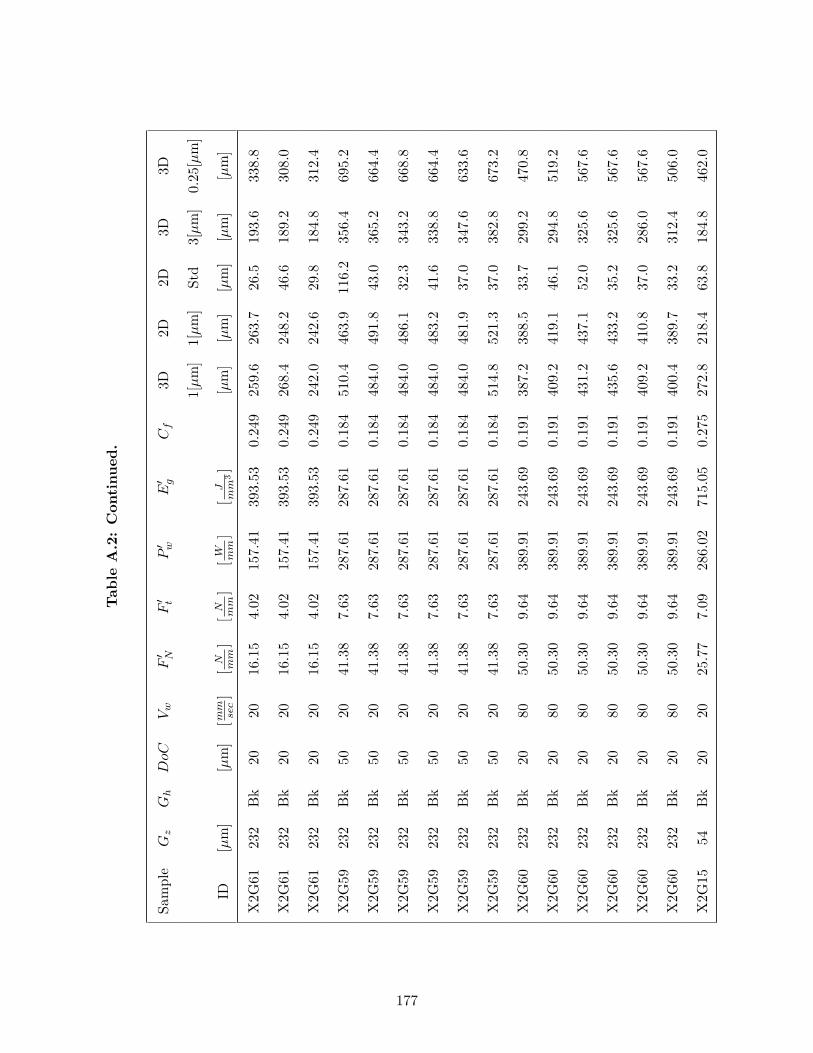
Tab
leA
.2:
Con
tinued
.
Sam
ple
Gz
Gh
DoC
Vw
F′ N
F′ t
P′ w
E′ g
Cf
3D2D
2D3D
3D
1[µm
]1[
µm
]St
d3[
µm
]0.
25[µ
m]
ID[µ
m]
[µm
][m
mse
c]
[N mm
][
N mm
][
W mm
][
Jm
m3]
[µm
][µ
m]
[µm
][µ
m]
[µm
]
X2G
6123
2B
k20
2016
.15
4.02
157.
4139
3.53
0.24
925
9.6
263.
726
.519
3.6
338.
8
X2G
6123
2B
k20
2016
.15
4.02
157.
4139
3.53
0.24
926
8.4
248.
246
.618
9.2
308.
0
X2G
6123
2B
k20
2016
.15
4.02
157.
4139
3.53
0.24
924
2.0
242.
629
.818
4.8
312.
4
X2G
5923
2B
k50
2041
.38
7.63
287.
6128
7.61
0.18
451
0.4
463.
911
6.2
356.
469
5.2
X2G
5923
2B
k50
2041
.38
7.63
287.
6128
7.61
0.18
448
4.0
491.
843
.036
5.2
664.
4
X2G
5923
2B
k50
2041
.38
7.63
287.
6128
7.61
0.18
448
4.0
486.
132
.334
3.2
668.
8
X2G
5923
2B
k50
2041
.38
7.63
287.
6128
7.61
0.18
448
4.0
483.
241
.633
8.8
664.
4
X2G
5923
2B
k50
2041
.38
7.63
287.
6128
7.61
0.18
448
4.0
481.
937
.034
7.6
633.
6
X2G
5923
2B
k50
2041
.38
7.63
287.
6128
7.61
0.18
451
4.8
521.
337
.038
2.8
673.
2
X2G
6023
2B
k20
8050
.30
9.64
389.
9124
3.69
0.19
138
7.2
388.
533
.729
9.2
470.
8
X2G
6023
2B
k20
8050
.30
9.64
389.
9124
3.69
0.19
140
9.2
419.
146
.129
4.8
519.
2
X2G
6023
2B
k20
8050
.30
9.64
389.
9124
3.69
0.19
143
1.2
437.
152
.032
5.6
567.
6
X2G
6023
2B
k20
8050
.30
9.64
389.
9124
3.69
0.19
143
5.6
433.
235
.232
5.6
567.
6
X2G
6023
2B
k20
8050
.30
9.64
389.
9124
3.69
0.19
140
9.2
410.
837
.028
6.0
567.
6
X2G
6023
2B
k20
8050
.30
9.64
389.
9124
3.69
0.19
140
0.4
389.
733
.231
2.4
506.
0
X2G
1554
Bk
2020
25.7
77.
0928
6.02
715.
050.
275
272.
821
8.4
63.8
184.
846
2.0
177
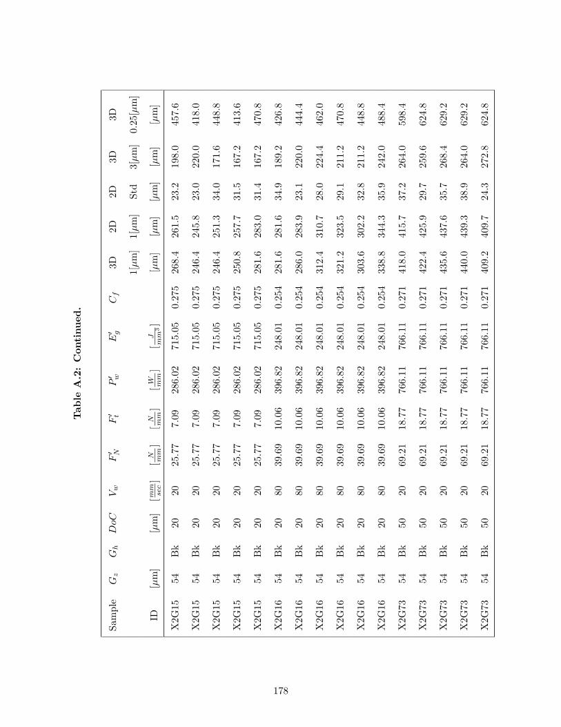
Tab
leA
.2:
Con
tinued
.
Sam
ple
Gz
Gh
DoC
Vw
F′ N
F′ t
P′ w
E′ g
Cf
3D2D
2D3D
3D
1[µm
]1[
µm
]St
d3[
µm
]0.
25[µ
m]
ID[µ
m]
[µm
][m
mse
c]
[N mm
][
N mm
][
W mm
][
Jm
m3]
[µm
][µ
m]
[µm
][µ
m]
[µm
]
X2G
1554
Bk
2020
25.7
77.
0928
6.02
715.
050.
275
268.
426
1.5
23.2
198.
045
7.6
X2G
1554
Bk
2020
25.7
77.
0928
6.02
715.
050.
275
246.
424
5.8
23.0
220.
041
8.0
X2G
1554
Bk
2020
25.7
77.
0928
6.02
715.
050.
275
246.
425
1.3
34.0
171.
644
8.8
X2G
1554
Bk
2020
25.7
77.
0928
6.02
715.
050.
275
250.
825
7.7
31.5
167.
241
3.6
X2G
1554
Bk
2020
25.7
77.
0928
6.02
715.
050.
275
281.
628
3.0
31.4
167.
247
0.8
X2G
1654
Bk
2080
39.6
910
.06
396.
8224
8.01
0.25
428
1.6
281.
634
.918
9.2
426.
8
X2G
1654
Bk
2080
39.6
910
.06
396.
8224
8.01
0.25
428
6.0
283.
923
.122
0.0
444.
4
X2G
1654
Bk
2080
39.6
910
.06
396.
8224
8.01
0.25
431
2.4
310.
728
.022
4.4
462.
0
X2G
1654
Bk
2080
39.6
910
.06
396.
8224
8.01
0.25
432
1.2
323.
529
.121
1.2
470.
8
X2G
1654
Bk
2080
39.6
910
.06
396.
8224
8.01
0.25
430
3.6
302.
232
.821
1.2
448.
8
X2G
1654
Bk
2080
39.6
910
.06
396.
8224
8.01
0.25
433
8.8
344.
335
.924
2.0
488.
4
X2G
7354
Bk
5020
69.2
118
.77
766.
1176
6.11
0.27
141
8.0
415.
737
.226
4.0
598.
4
X2G
7354
Bk
5020
69.2
118
.77
766.
1176
6.11
0.27
142
2.4
425.
929
.725
9.6
624.
8
X2G
7354
Bk
5020
69.2
118
.77
766.
1176
6.11
0.27
143
5.6
437.
635
.726
8.4
629.
2
X2G
7354
Bk
5020
69.2
118
.77
766.
1176
6.11
0.27
144
0.0
439.
338
.926
4.0
629.
2
X2G
7354
Bk
5020
69.2
118
.77
766.
1176
6.11
0.27
140
9.2
409.
724
.327
2.8
624.
8
178

Tab
leA
.2:
Con
tinued
.
Sam
ple
Gz
Gh
DoC
Vw
F′ N
F′ t
P′ w
E′ g
Cf
3D2D
2D3D
3D
1[µm
]1[
µm
]St
d3[
µm
]0.
25[µ
m]
ID[µ
m]
[µm
][m
mse
c]
[N mm
][
N mm
][
W mm
][
Jm
m3]
[µm
][µ
m]
[µm
][µ
m]
[µm
]
X2G
7354
Bk
5020
69.2
118
.77
766.
1176
6.11
0.27
142
6.8
422.
726
.030
8.0
580.
8
X2G
6254
Ag
2080
29.2
68.
3432
6.84
204.
280.
285
206.
819
7.1
16.9
127.
633
8.8
X2G
6254
Ag
2080
29.2
68.
3432
6.84
204.
280.
285
189.
218
4.1
46.8
123.
236
9.6
X2G
6254
Ag
2080
29.2
68.
3432
6.84
204.
280.
285
220.
015
9.8
46.8
123.
236
9.6
X2G
6254
Ag
2080
29.2
68.
3432
6.84
204.
280.
285
215.
617
0.7
61.0
132.
037
8.4
X2G
6254
Ag
2080
29.2
68.
3432
6.84
204.
280.
285
202.
419
5.5
25.5
132.
036
5.2
X2G
6254
Ag
2080
29.2
68.
3432
6.84
204.
280.
285
193.
619
5.7
19.9
114.
436
0.8
X2G
7154
Ag
2020
26.4
37.
6930
8.14
770.
350.
291
193.
618
4.4
19.9
114.
439
1.6
X2G
7154
Ag
2020
26.4
37.
6930
8.14
770.
350.
291
189.
218
5.6
22.3
162.
837
8.4
X2G
7154
Ag
2020
26.4
37.
6930
8.14
770.
350.
291
184.
817
8.6
22.5
114.
434
7.6
X2G
7154
Ag
2020
26.4
37.
6930
8.14
770.
350.
291
193.
619
0.8
20.1
123.
237
4.0
X2G
7154
Ag
2020
26.4
37.
6930
8.14
770.
350.
291
189.
217
4.8
21.2
140.
829
9.2
X2G
7154
Ag
2020
26.4
37.
6930
8.14
770.
350.
291
198.
019
4.5
21.4
127.
639
1.6
X2G
7054
Ag
5020
42.0
011
.73
479.
3447
9.34
0.27
931
6.8
318.
224
.317
6.0
536.
8
X2G
7054
Ag
5020
42.0
011
.73
479.
3447
9.34
0.27
933
0.0
327.
025
.217
6.0
545.
6
X2G
7054
Ag
5020
42.0
011
.73
479.
3447
9.34
0.27
936
0.8
323.
686
.323
3.2
554.
4
179
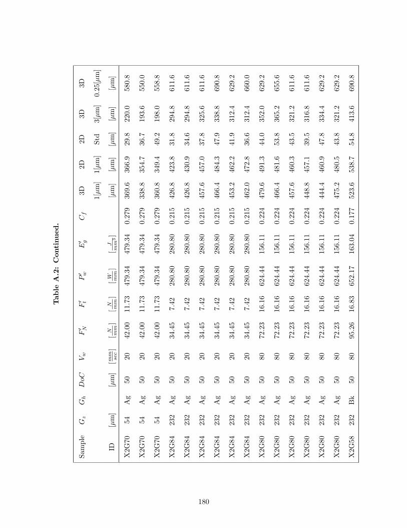
Tab
leA
.2:
Con
tinued
.
Sam
ple
Gz
Gh
DoC
Vw
F′ N
F′ t
P′ w
E′ g
Cf
3D2D
2D3D
3D
1[µm
]1[
µm
]St
d3[
µm
]0.
25[µ
m]
ID[µ
m]
[µm
][m
mse
c]
[N mm
][
N mm
][
W mm
][
Jm
m3]
[µm
][µ
m]
[µm
][µ
m]
[µm
]
X2G
7054
Ag
5020
42.0
011
.73
479.
3447
9.34
0.27
936
9.6
366.
929
.822
0.0
580.
8
X2G
7054
Ag
5020
42.0
011
.73
479.
3447
9.34
0.27
933
8.8
354.
736
.719
3.6
550.
0
X2G
7054
Ag
5020
42.0
011
.73
479.
3447
9.34
0.27
936
0.8
349.
449
.219
8.0
558.
8
X2G
8423
2A
g50
2034
.45
7.42
280.
8028
0.80
0.21
542
6.8
423.
831
.829
4.8
611.
6
X2G
8423
2A
g50
2034
.45
7.42
280.
8028
0.80
0.21
542
6.8
430.
934
.629
4.8
611.
6
X2G
8423
2A
g50
2034
.45
7.42
280.
8028
0.80
0.21
545
7.6
457.
037
.832
5.6
611.
6
X2G
8423
2A
g50
2034
.45
7.42
280.
8028
0.80
0.21
546
6.4
484.
347
.933
8.8
690.
8
X2G
8423
2A
g50
2034
.45
7.42
280.
8028
0.80
0.21
545
3.2
462.
241
.931
2.4
629.
2
X2G
8423
2A
g50
2034
.45
7.42
280.
8028
0.80
0.21
546
2.0
472.
836
.631
2.4
660.
0
X2G
8023
2A
g50
8072
.23
16.1
662
4.44
156.
110.
224
479.
649
1.3
44.0
352.
062
9.2
X2G
8023
2A
g50
8072
.23
16.1
662
4.44
156.
110.
224
466.
448
1.6
53.8
365.
265
5.6
X2G
8023
2A
g50
8072
.23
16.1
662
4.44
156.
110.
224
457.
646
0.3
43.5
321.
261
1.6
X2G
8023
2A
g50
8072
.23
16.1
662
4.44
156.
110.
224
448.
845
7.1
39.5
316.
861
1.6
X2G
8023
2A
g50
8072
.23
16.1
662
4.44
156.
110.
224
444.
446
0.9
47.8
334.
462
9.2
X2G
8023
2A
g50
8072
.23
16.1
662
4.44
156.
110.
224
475.
248
0.5
43.8
321.
262
9.2
X2G
5823
2B
k50
8095
.26
16.8
365
2.17
163.
040.
177
523.
653
8.7
54.8
413.
669
0.8
180
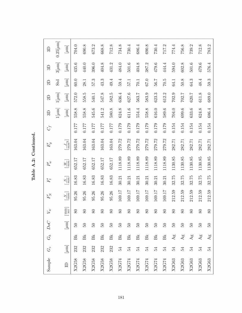
Tab
leA
.2:
Con
tinued
.
Sam
ple
Gz
Gh
DoC
Vw
F′ N
F′ t
P′ w
E′ g
Cf
3D2D
2D3D
3D
1[µm
]1[
µm
]St
d3[
µm
]0.
25[µ
m]
ID[µ
m]
[µm
][m
mse
c]
[N mm
][
N mm
][
W mm
][
Jm
m3]
[µm
][µ
m]
[µm
][µ
m]
[µm
]
X2G
5823
2B
k50
8095
.26
16.8
365
2.17
163.
040.
177
558.
857
2.0
60.0
435.
670
4.0
X2G
5823
2B
k50
8095
.26
16.8
365
2.17
163.
040.
177
558.
855
8.5
28.1
440.
069
0.8
X2G
5823
2B
k50
8095
.26
16.8
365
2.17
163.
040.
177
545.
654
0.1
57.3
396.
067
3.2
X2G
5823
2B
k50
8095
.26
16.8
365
2.17
163.
040.
177
541.
254
7.8
43.3
404.
866
8.8
X2G
5823
2B
k50
8095
.26
16.8
365
2.17
163.
040.
177
580.
858
2.5
49.4
431.
271
2.8
X2G
7454
Bk
5080
169.
1730
.21
1118
.89
279.
720.
179
624.
863
6.4
59.4
484.
073
4.8
X2G
7454
Bk
5080
169.
1730
.21
1118
.89
279.
720.
179
611.
662
7.6
57.1
501.
673
0.4
X2G
7454
Bk
5080
169.
1730
.21
1118
.89
279.
720.
179
554.
456
3.7
70.1
404.
868
6.4
X2G
7454
Bk
5080
169.
1730
.21
1118
.89
279.
720.
179
558.
858
3.9
67.0
387.
269
0.8
X2G
7454
Bk
5080
169.
1730
.21
1118
.89
279.
720.
179
616.
062
3.3
56.7
479.
673
0.4
X2G
7454
Bk
5080
169.
1730
.21
1118
.89
279.
720.
179
589.
661
2.2
70.5
444.
471
7.2
X2G
6354
Ag
5080
212.
5932
.75
1130
.85
282.
710.
154
704.
070
2.9
64.1
594.
077
4.4
X2G
6354
Ag
5080
212.
5932
.75
1130
.85
282.
710.
154
699.
670
2.7
50.8
602.
875
6.8
X2G
6354
Ag
5080
212.
5932
.75
1130
.85
282.
710.
154
633.
662
0.7
64.3
501.
673
9.2
X2G
6354
Ag
5080
212.
5932
.75
1130
.85
282.
710.
154
624.
861
1.8
48.4
479.
671
2.8
X2G
6354
Ag
5080
212.
5932
.75
1130
.85
282.
710.
154
686.
468
9.0
59.3
576.
478
3.2
181
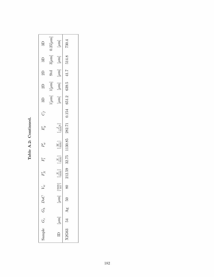
Tab
leA
.2:
Con
tinued
.
Sam
ple
Gz
Gh
DoC
Vw
F′ N
F′ t
P′ w
E′ g
Cf
3D2D
2D3D
3D
1[µm
]1[
µm
]St
d3[
µm
]0.
25[µ
m]
ID[µ
m]
[µm
][m
mse
c]
[N mm
][
N mm
][
W mm
][
Jm
m3]
[µm
][µ
m]
[µm
][µ
m]
[µm
]
X2G
6354
Ag
5080
212.
5932
.75
1130
.85
282.
710.
154
651.
263
9.5
41.7
514.
873
0.4
182

APPENDIX B
RESIDUAL STRESS MEASUREMENT RESULTS
183
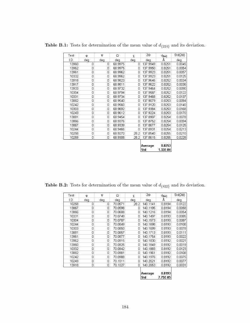
Table B.1: Tests for determination of the mean value of d224 and its deviation.
Table B.2: Tests for determination of the mean value of d422 and its deviation.
184
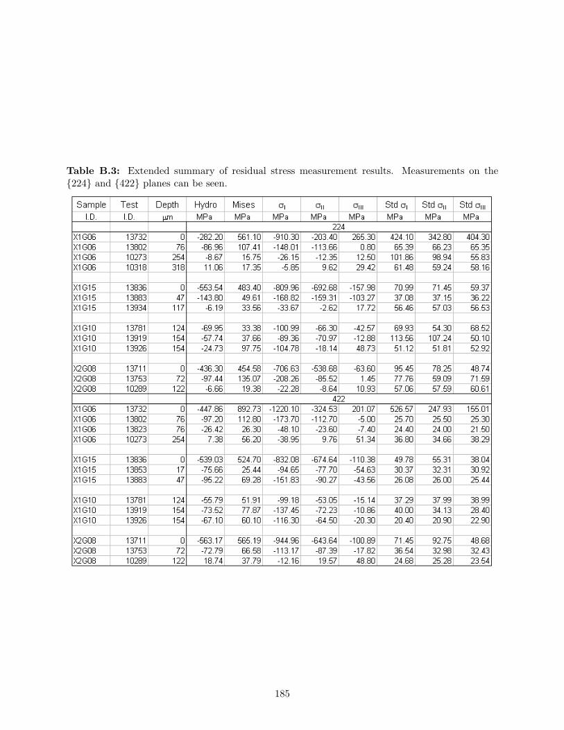
Table B.3: Extended summary of residual stress measurement results. Measurements on the224 and 422 planes can be seen.
185
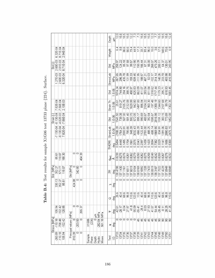
Tab
leB
.4:
Tes
tre
sult
sfo
rsa
mpl
eX
1G06
test
1373
3pl
ane2
24.
Surf
ace.
186
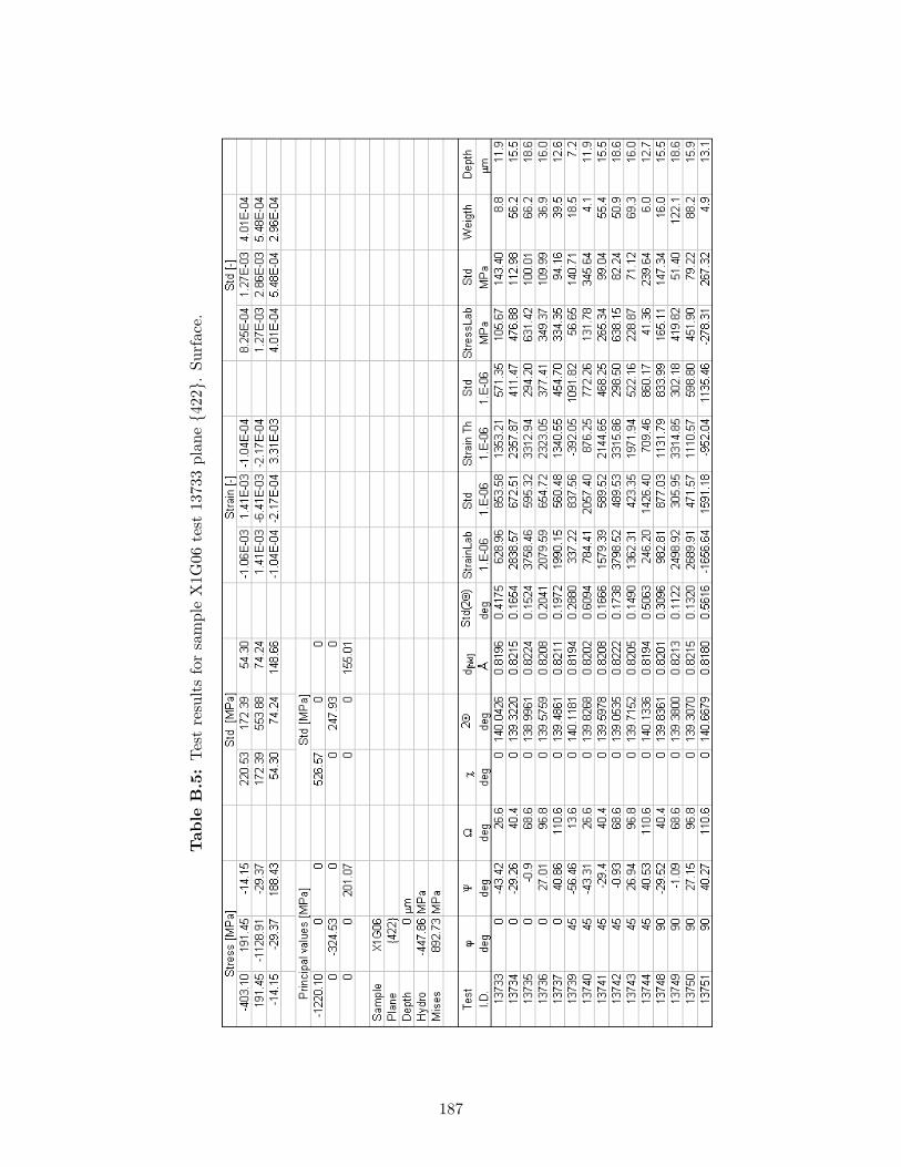
Tab
leB
.5:
Tes
tre
sult
sfo
rsa
mpl
eX
1G06
test
1373
3pl
ane4
22.
Surf
ace.
187
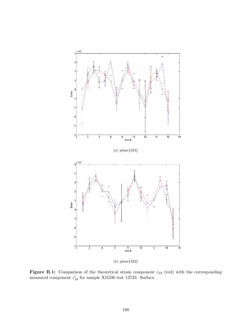
(a) plane224
(b) plane422
Figure B.1: Comparison of the theoretical strain component ε33 (red) with the correspondingmeasured component ε′33 for sample X1G06 test 13733. Surface.
188

Tab
leB
.6:
Tes
tre
sult
sfo
rsa
mpl
eX
1G06
test
1380
2pl
ane2
24.
76µm
subs
urfa
ce.
189
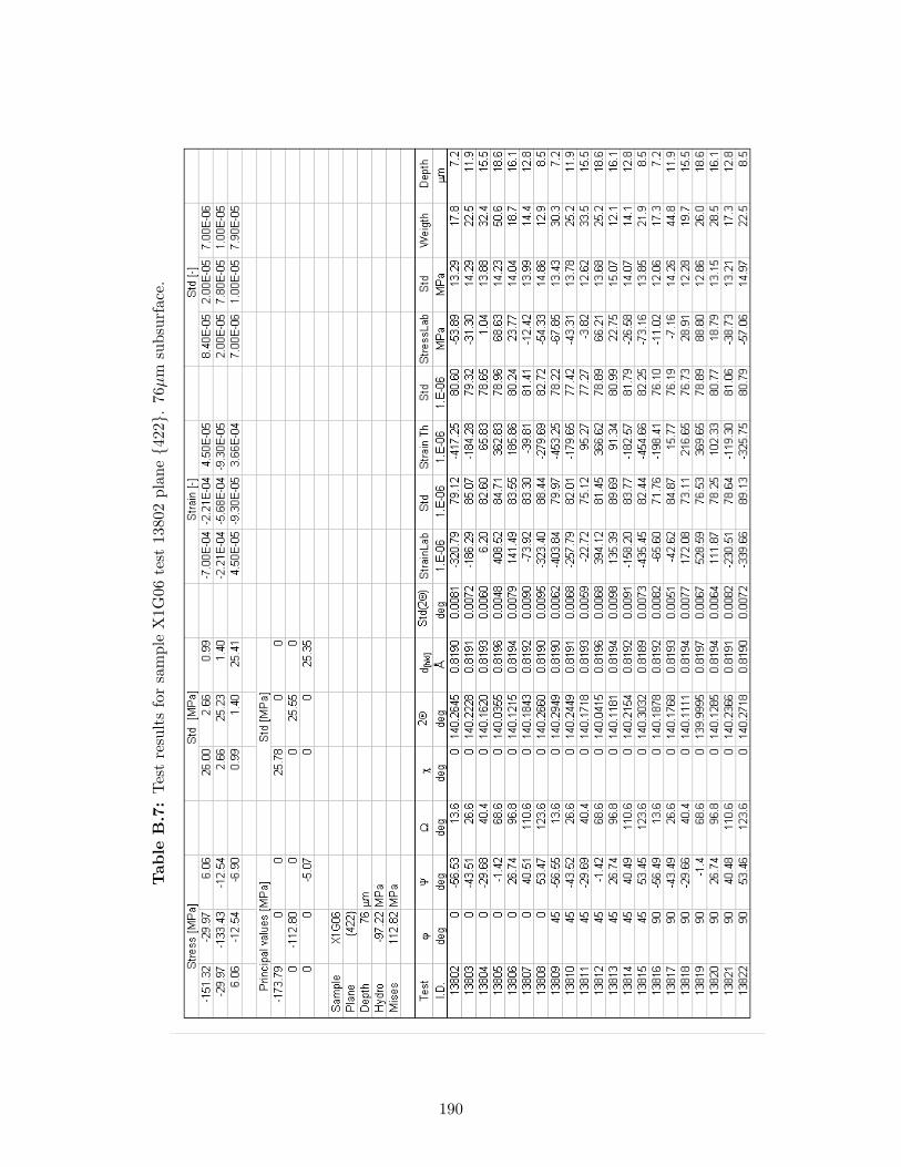
Tab
leB
.7:
Tes
tre
sult
sfo
rsa
mpl
eX
1G06
test
1380
2pl
ane4
22.
76µm
subs
urfa
ce.
190
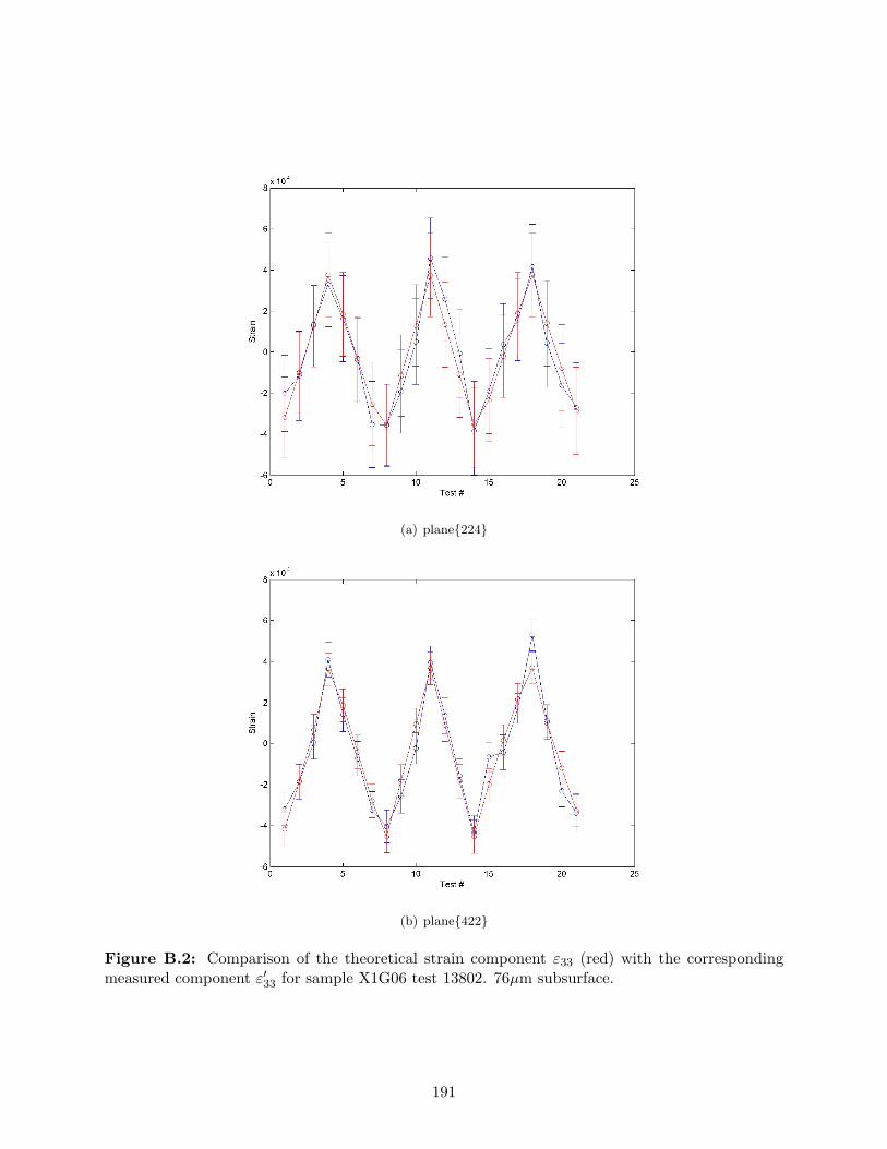
(a) plane224
(b) plane422
Figure B.2: Comparison of the theoretical strain component ε33 (red) with the correspondingmeasured component ε′33 for sample X1G06 test 13802. 76µm subsurface.
191

Tab
leB
.8:
Tes
tre
sult
sfo
rsa
mpl
eX
1G06
test
1382
3pl
ane4
22.
76µm
subs
urfa
ce.
192
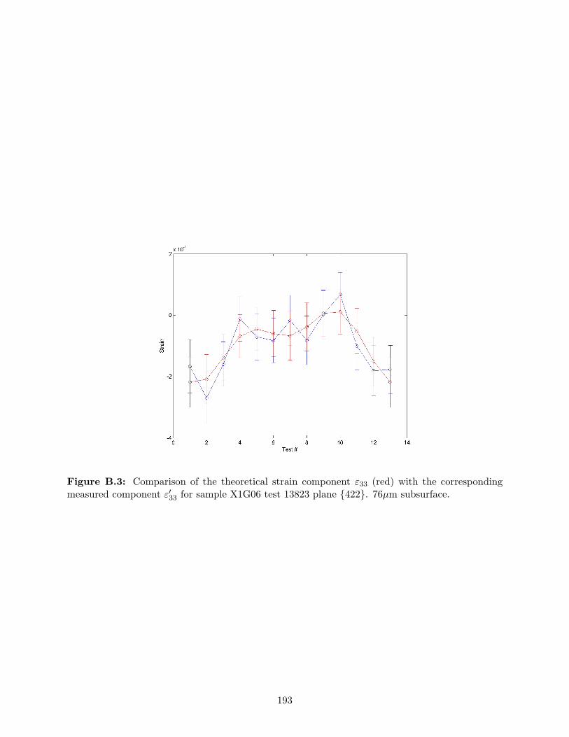
Figure B.3: Comparison of the theoretical strain component ε33 (red) with the correspondingmeasured component ε′33 for sample X1G06 test 13823 plane 422. 76µm subsurface.
193
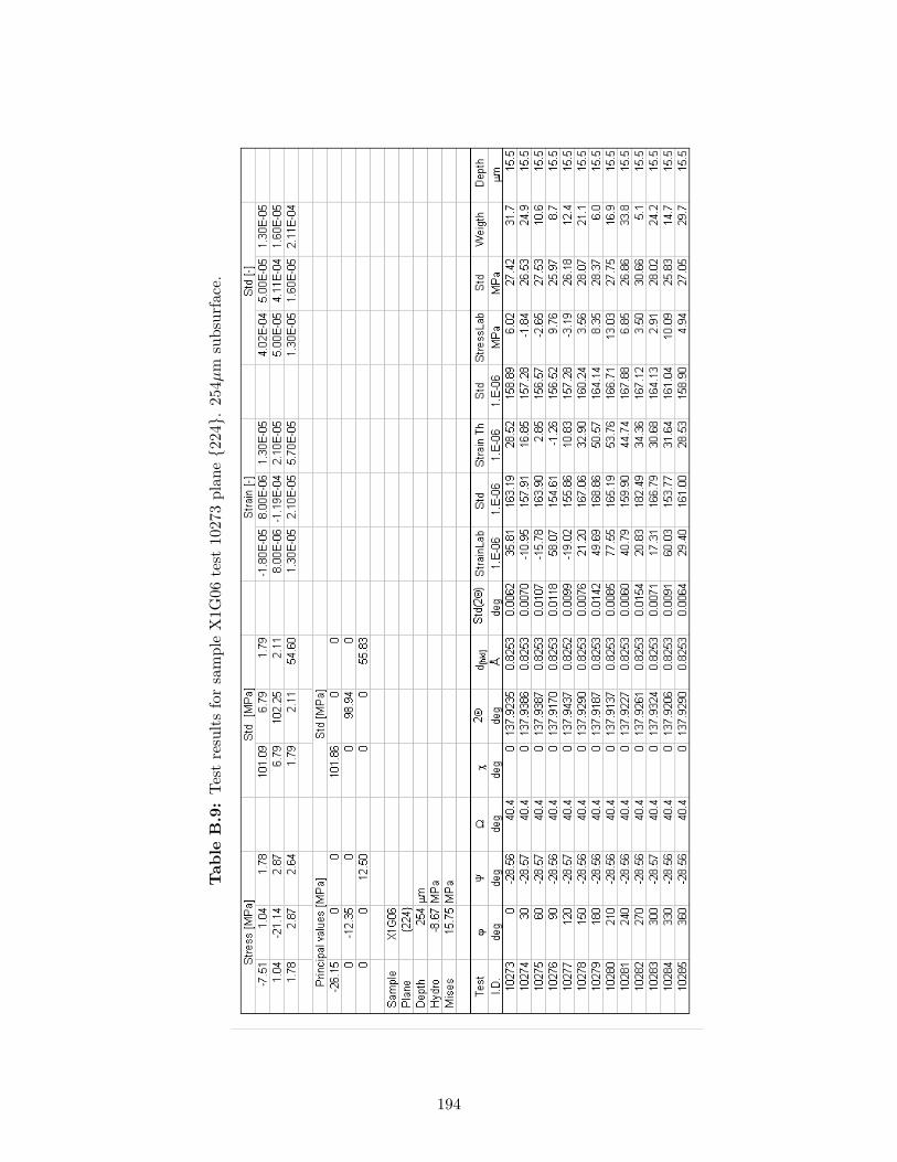
Tab
leB
.9:
Tes
tre
sult
sfo
rsa
mpl
eX
1G06
test
1027
3pl
ane2
24.
254µ
msu
bsur
face
.
194
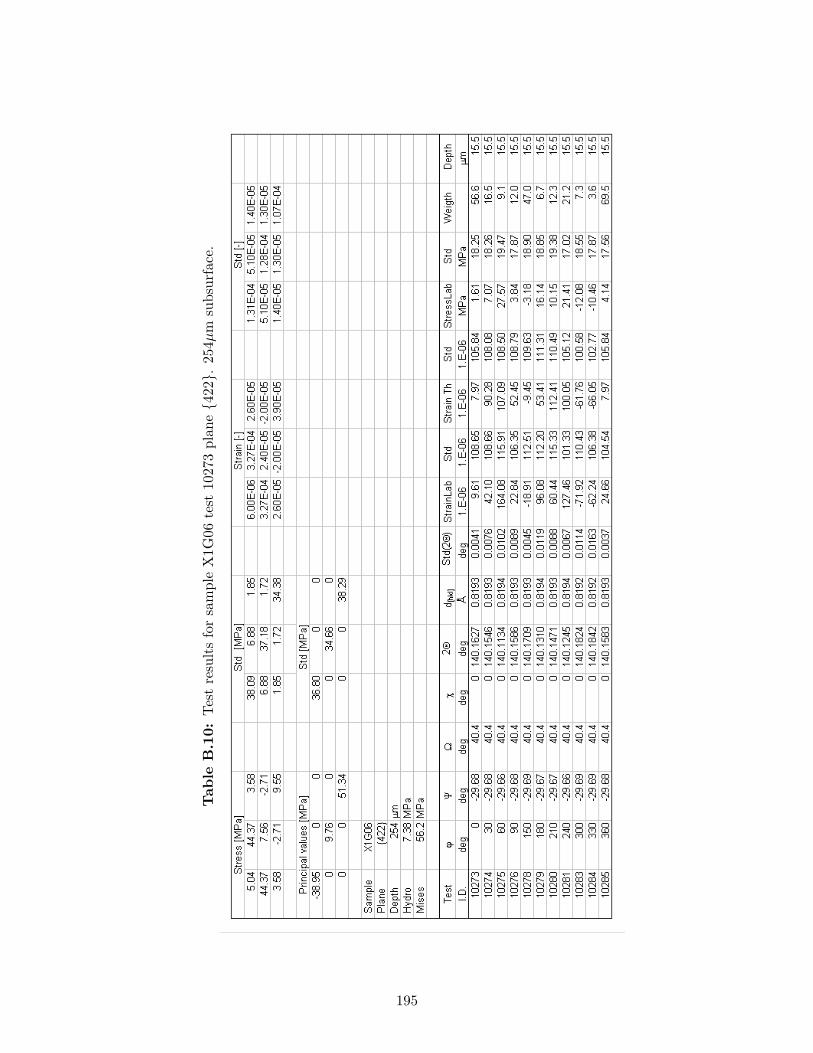
Tab
leB
.10:
Tes
tre
sult
sfo
rsa
mpl
eX
1G06
test
1027
3pl
ane4
22.
254µ
msu
bsur
face
.
195
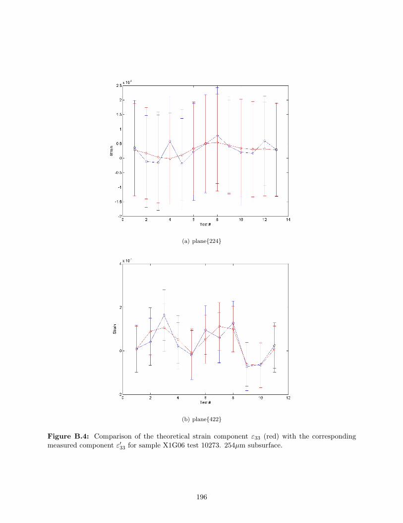
(a) plane224
(b) plane422
Figure B.4: Comparison of the theoretical strain component ε33 (red) with the correspondingmeasured component ε′33 for sample X1G06 test 10273. 254µm subsurface.
196
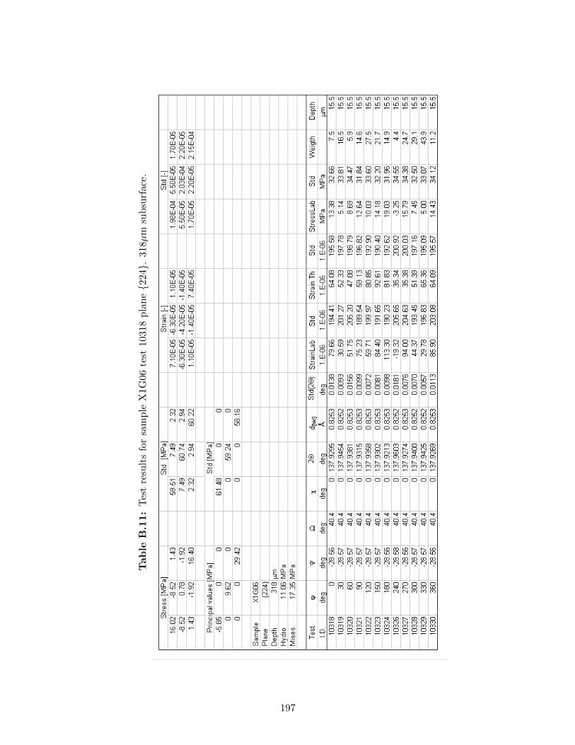
Tab
leB
.11:
Tes
tre
sult
sfo
rsa
mpl
eX
1G06
test
1031
8pl
ane2
24.
318µ
msu
bsur
face
.
197
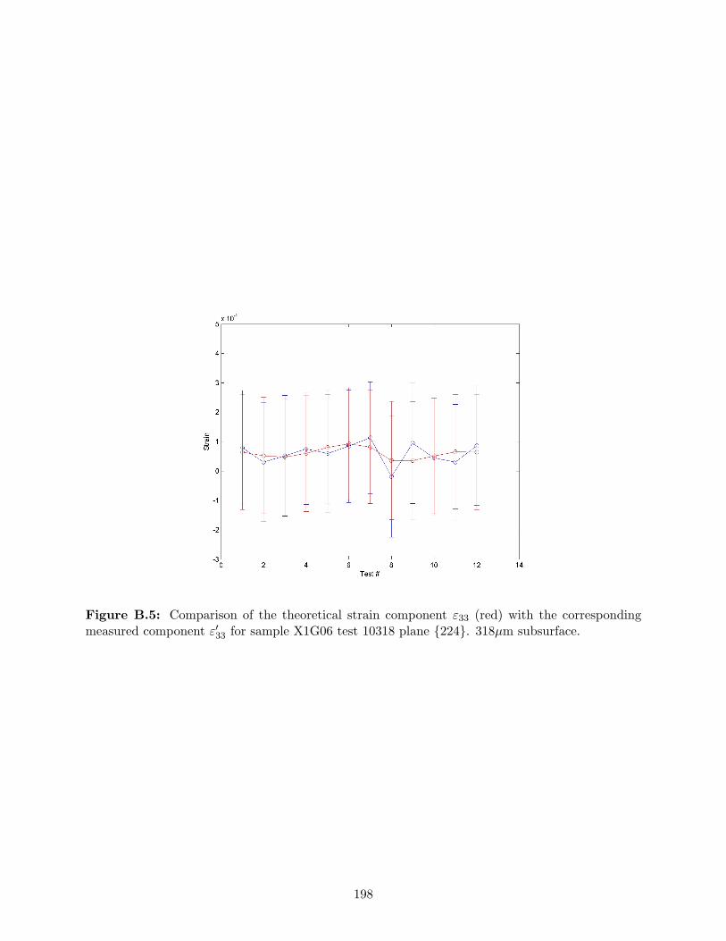
Figure B.5: Comparison of the theoretical strain component ε33 (red) with the correspondingmeasured component ε′33 for sample X1G06 test 10318 plane 224. 318µm subsurface.
198

Tab
leB
.12:
Tes
tre
sult
sfo
rsa
mpl
eX
1G15
test
1383
6pl
ane2
24.
Surf
ace.
199
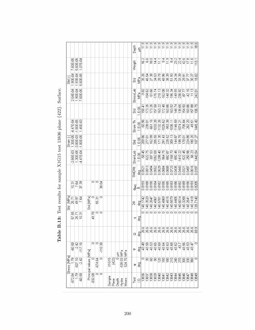
Tab
leB
.13:
Tes
tre
sult
sfo
rsa
mpl
eX
1G15
test
1383
6pl
ane4
22.
Surf
ace.
200
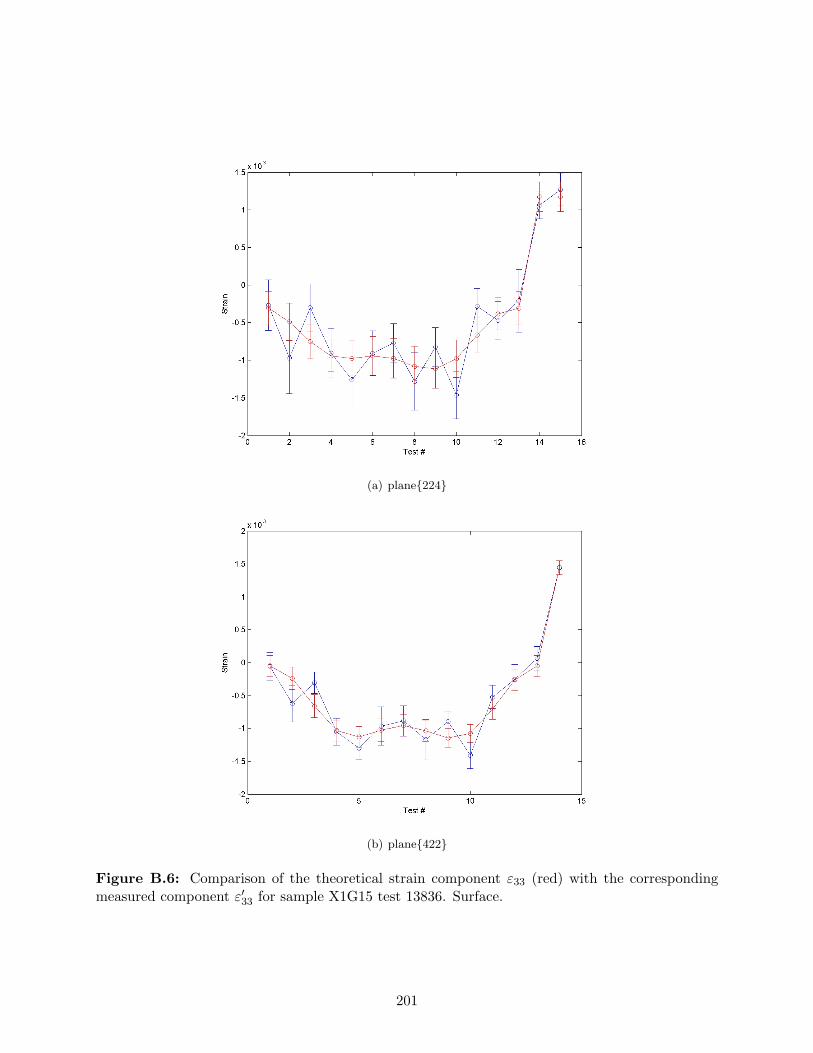
(a) plane224
(b) plane422
Figure B.6: Comparison of the theoretical strain component ε33 (red) with the correspondingmeasured component ε′33 for sample X1G15 test 13836. Surface.
201
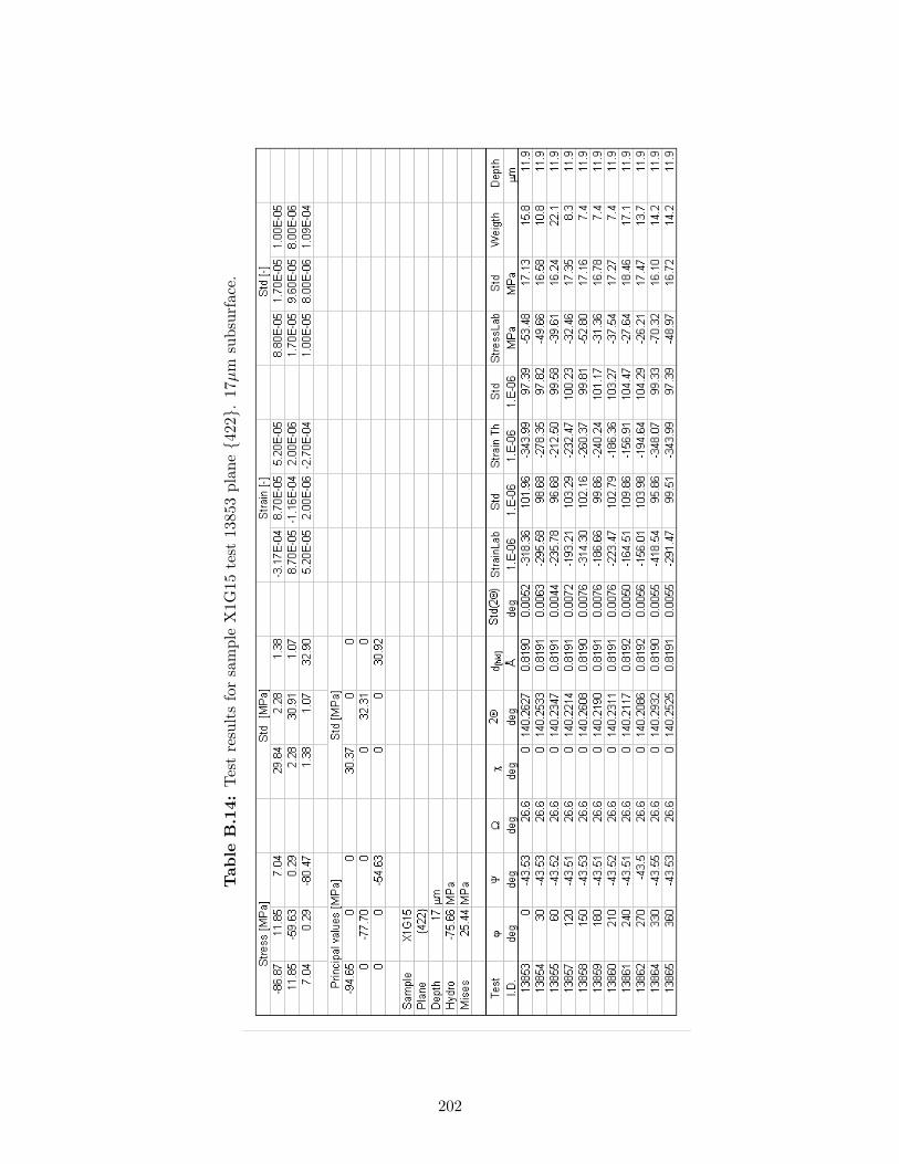
Tab
leB
.14:
Tes
tre
sult
sfo
rsa
mpl
eX
1G15
test
1385
3pl
ane4
22.
17µm
subs
urfa
ce.
202
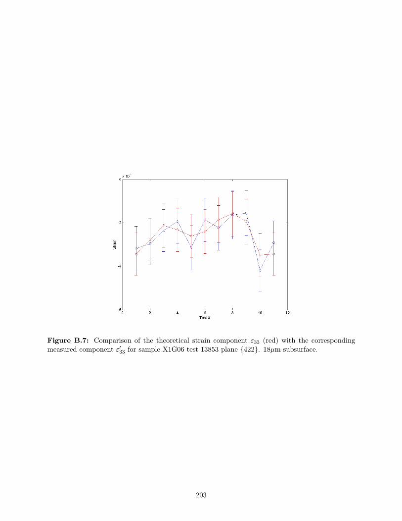
Figure B.7: Comparison of the theoretical strain component ε33 (red) with the correspondingmeasured component ε′33 for sample X1G06 test 13853 plane 422. 18µm subsurface.
203

Tab
leB
.15:
Tes
tre
sult
sfo
rsa
mpl
eX
1G15
test
1388
3pl
ane2
24.
47µm
subs
urfa
ce.
204
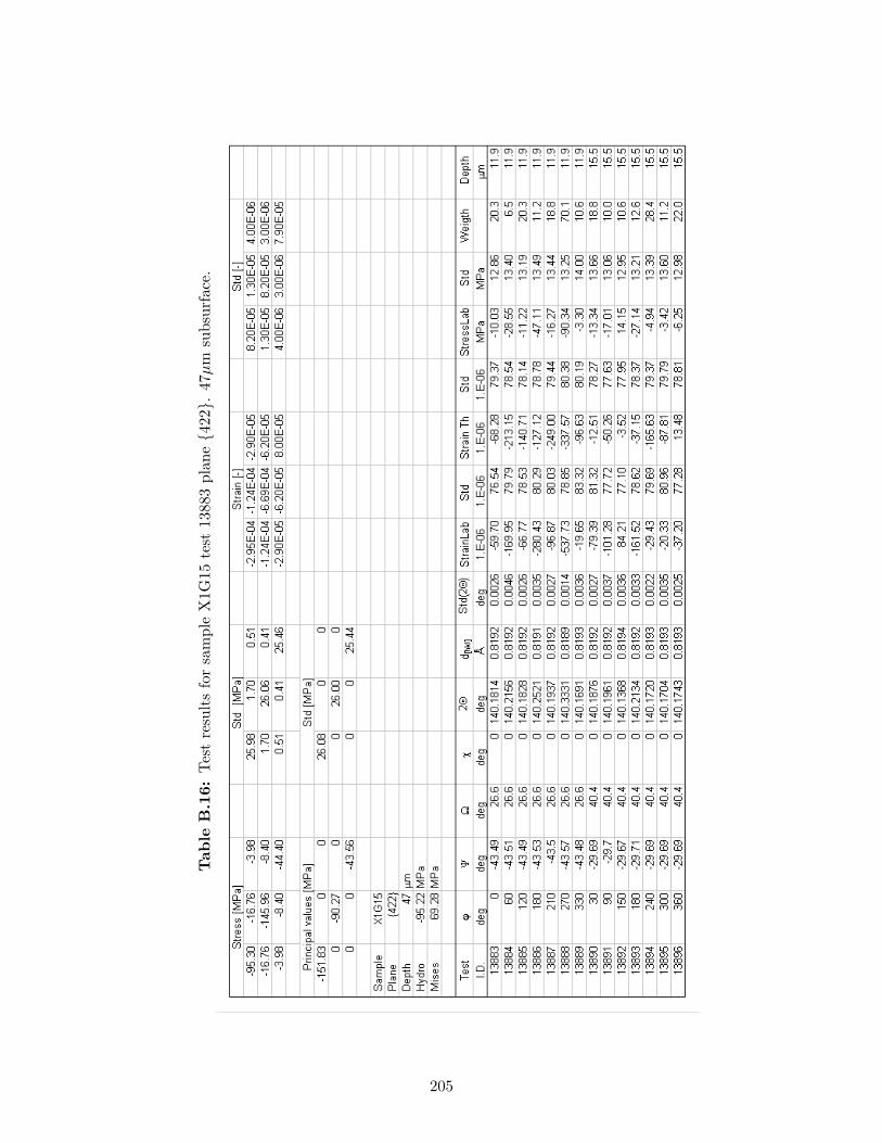
Tab
leB
.16:
Tes
tre
sult
sfo
rsa
mpl
eX
1G15
test
1388
3pl
ane4
22.
47µm
subs
urfa
ce.
205
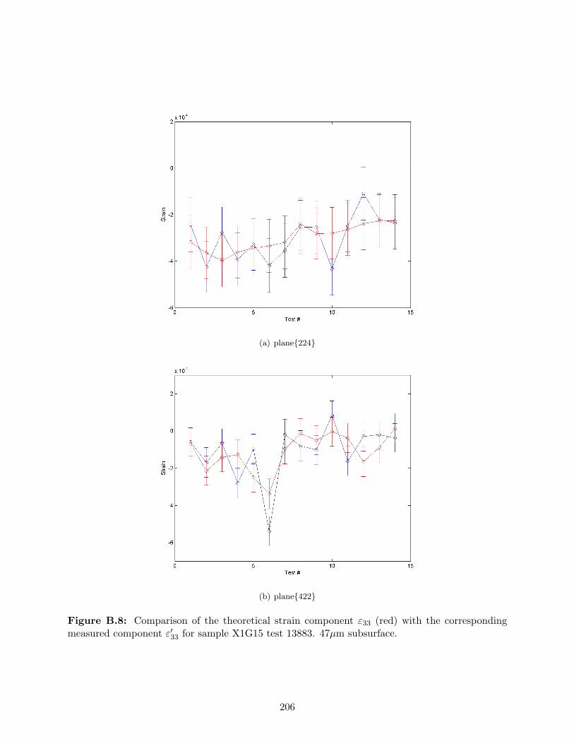
(a) plane224
(b) plane422
Figure B.8: Comparison of the theoretical strain component ε33 (red) with the correspondingmeasured component ε′33 for sample X1G15 test 13883. 47µm subsurface.
206
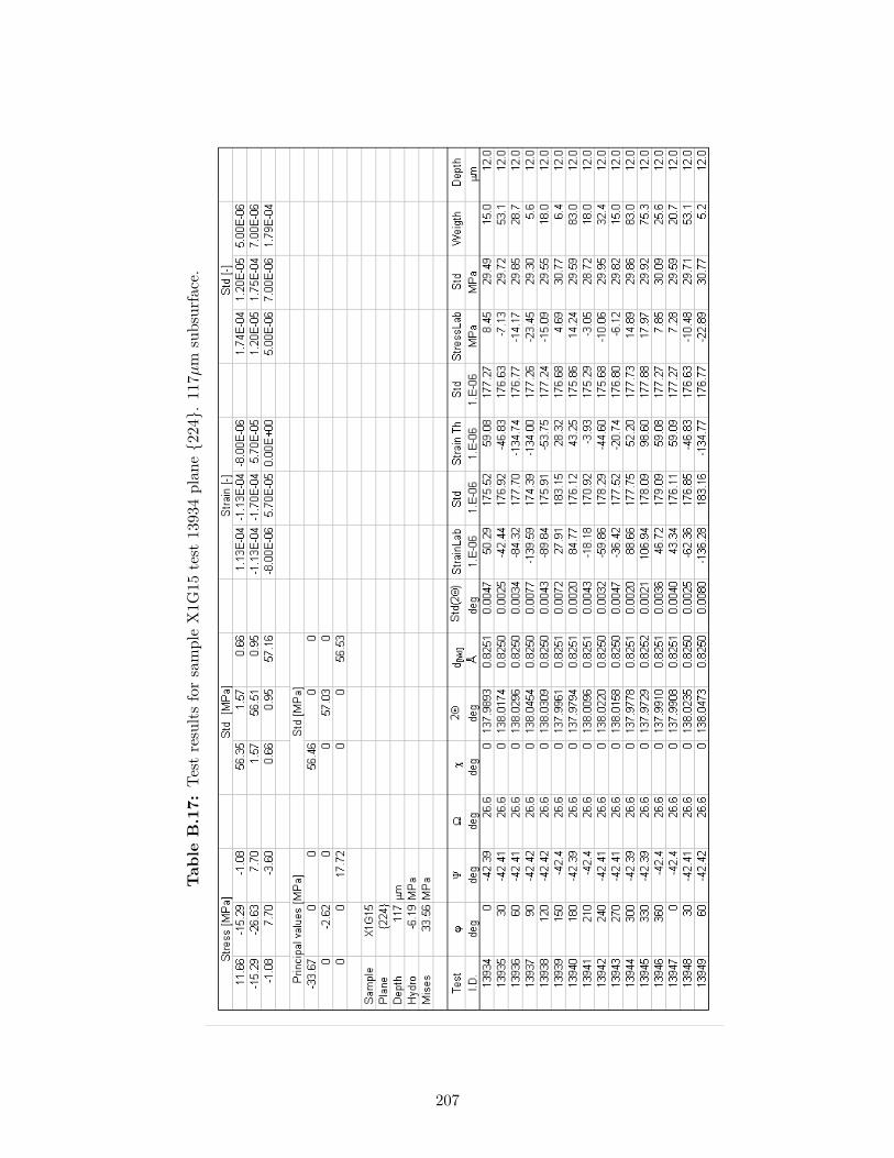
Tab
leB
.17:
Tes
tre
sult
sfo
rsa
mpl
eX
1G15
test
1393
4pl
ane2
24.
117µ
msu
bsur
face
.
207
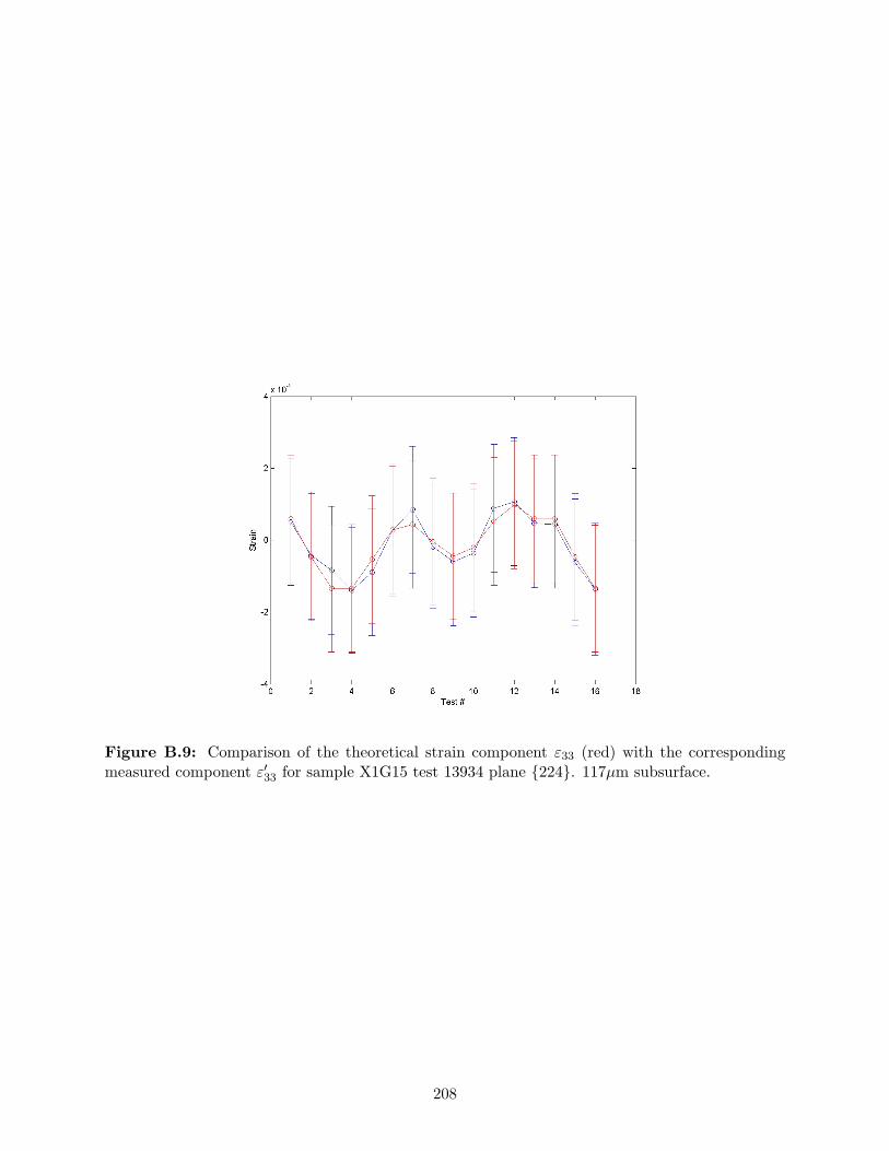
Figure B.9: Comparison of the theoretical strain component ε33 (red) with the correspondingmeasured component ε′33 for sample X1G15 test 13934 plane 224. 117µm subsurface.
208

Tab
leB
.18:
Tes
tre
sult
sfo
rsa
mpl
eX
1G10
test
1378
1pl
ane2
24.
124µ
msu
bsur
face
.
209
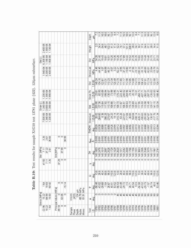
Tab
leB
.19:
Tes
tre
sult
sfo
rsa
mpl
eX
1G10
test
1378
1pl
ane4
22.
124µ
msu
bsur
face
.
210
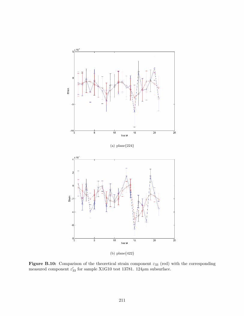
(a) plane224
(b) plane422
Figure B.10: Comparison of the theoretical strain component ε33 (red) with the correspondingmeasured component ε′33 for sample X1G10 test 13781. 124µm subsurface.
211

Tab
leB
.20:
Tes
tre
sult
sfo
rsa
mpl
eX
1G10
test
1391
9pl
ane2
24.
154µ
msu
bsur
face
.
212
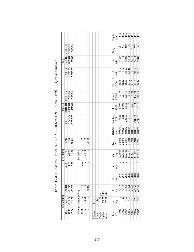
Tab
leB
.21:
Tes
tre
sult
sfo
rsa
mpl
eX
1G10
test
1391
9pl
ane4
22.
154µ
msu
bsur
face
.
213
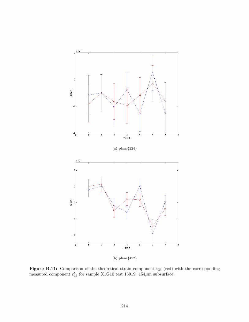
(a) plane224
(b) plane422
Figure B.11: Comparison of the theoretical strain component ε33 (red) with the correspondingmeasured component ε′33 for sample X1G10 test 13919. 154µm subsurface.
214

Tab
leB
.22:
Tes
tre
sult
sfo
rsa
mpl
eX
1G10
test
1392
6pl
ane2
24.
154µ
msu
bsur
face
.
215
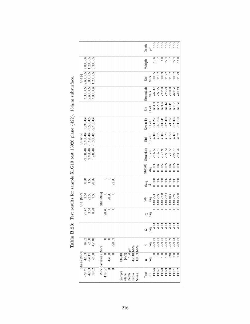
Tab
leB
.23:
Tes
tre
sult
sfo
rsa
mpl
eX
1G10
test
1392
6pl
ane4
22.
154µ
msu
bsur
face
.
216
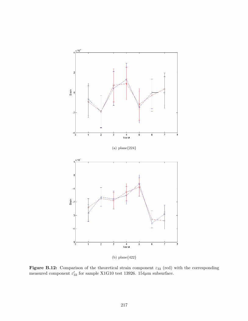
(a) plane224
(b) plane422
Figure B.12: Comparison of the theoretical strain component ε33 (red) with the correspondingmeasured component ε′33 for sample X1G10 test 13926. 154µm subsurface.
217
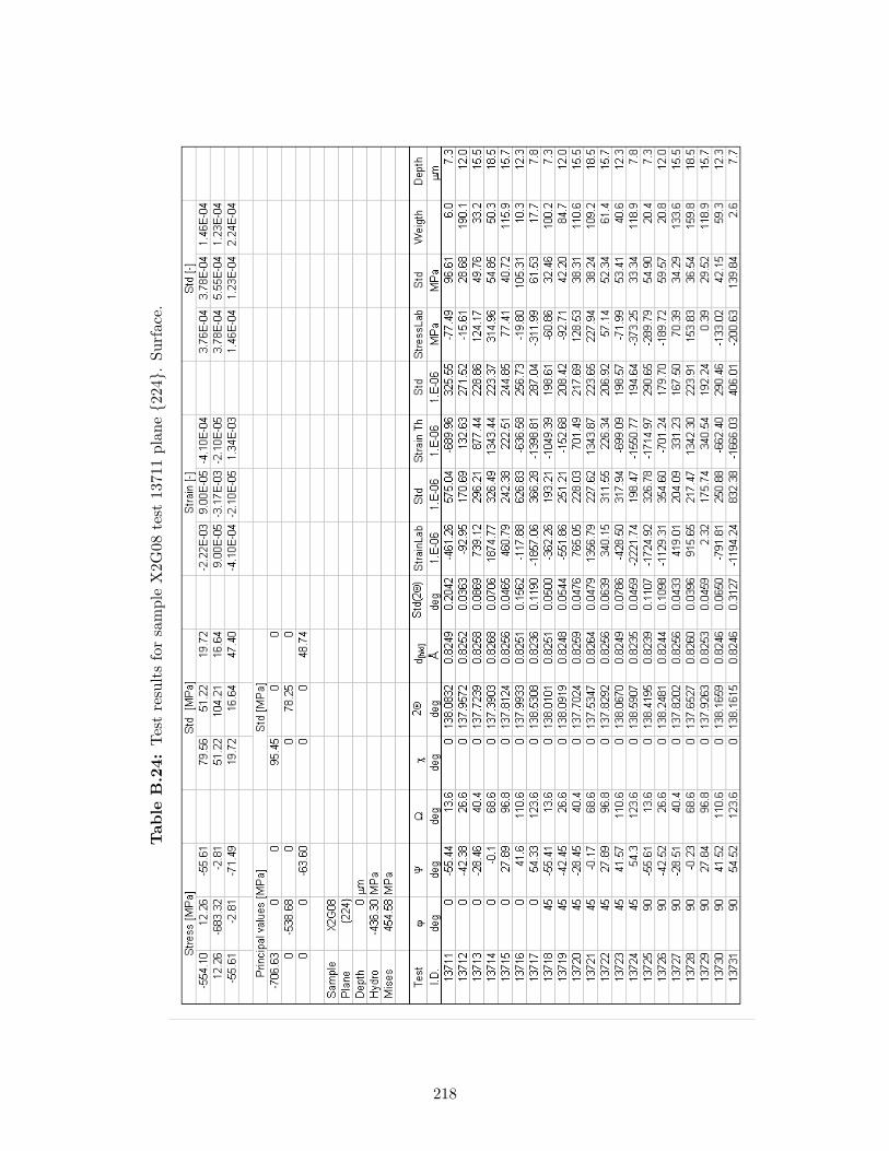
Tab
leB
.24:
Tes
tre
sult
sfo
rsa
mpl
eX
2G08
test
1371
1pl
ane2
24.
Surf
ace.
218

Tab
leB
.25:
Tes
tre
sult
sfo
rsa
mpl
eX
2G08
test
1371
1pl
ane4
22.
Surf
ace.
219
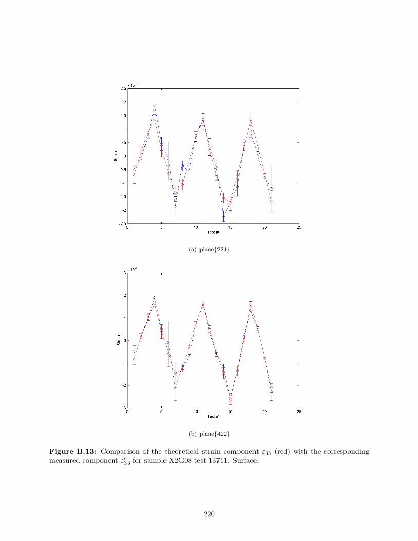
(a) plane224
(b) plane422
Figure B.13: Comparison of the theoretical strain component ε33 (red) with the correspondingmeasured component ε′33 for sample X2G08 test 13711. Surface.
220
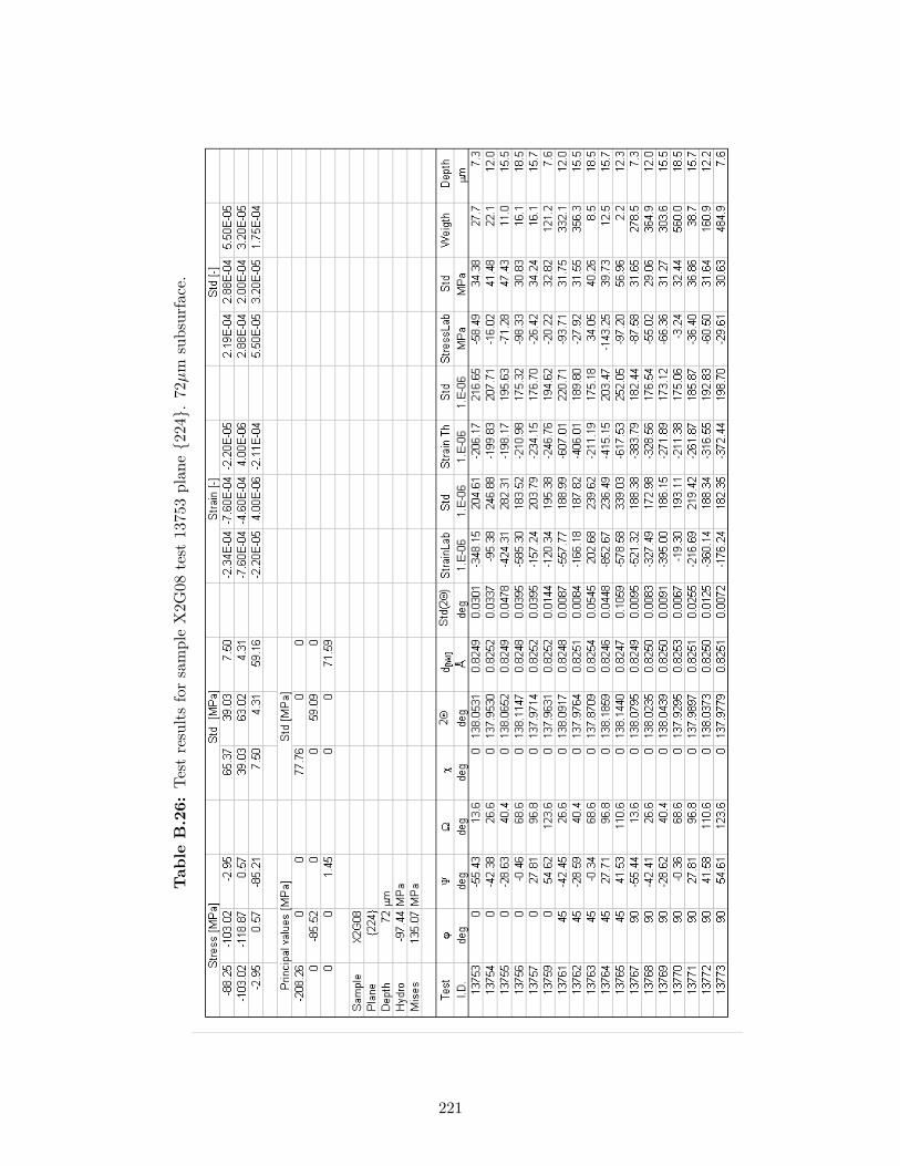
Tab
leB
.26:
Tes
tre
sult
sfo
rsa
mpl
eX
2G08
test
1375
3pl
ane2
24.
72µm
subs
urfa
ce.
221

Tab
leB
.27:
Tes
tre
sult
sfo
rsa
mpl
eX
2G08
test
1375
3pl
ane4
22.
72µm
subs
urfa
ce.
222
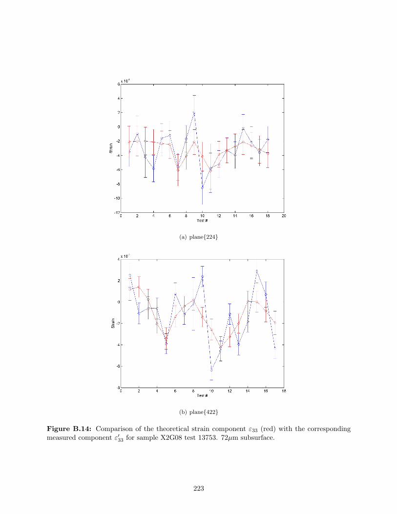
(a) plane224
(b) plane422
Figure B.14: Comparison of the theoretical strain component ε33 (red) with the correspondingmeasured component ε′33 for sample X2G08 test 13753. 72µm subsurface.
223

Tab
leB
.28:
Tes
tre
sult
sfo
rsa
mpl
eX
2G08
test
1028
9pl
ane2
24.
122µ
msu
bsur
face
.
224
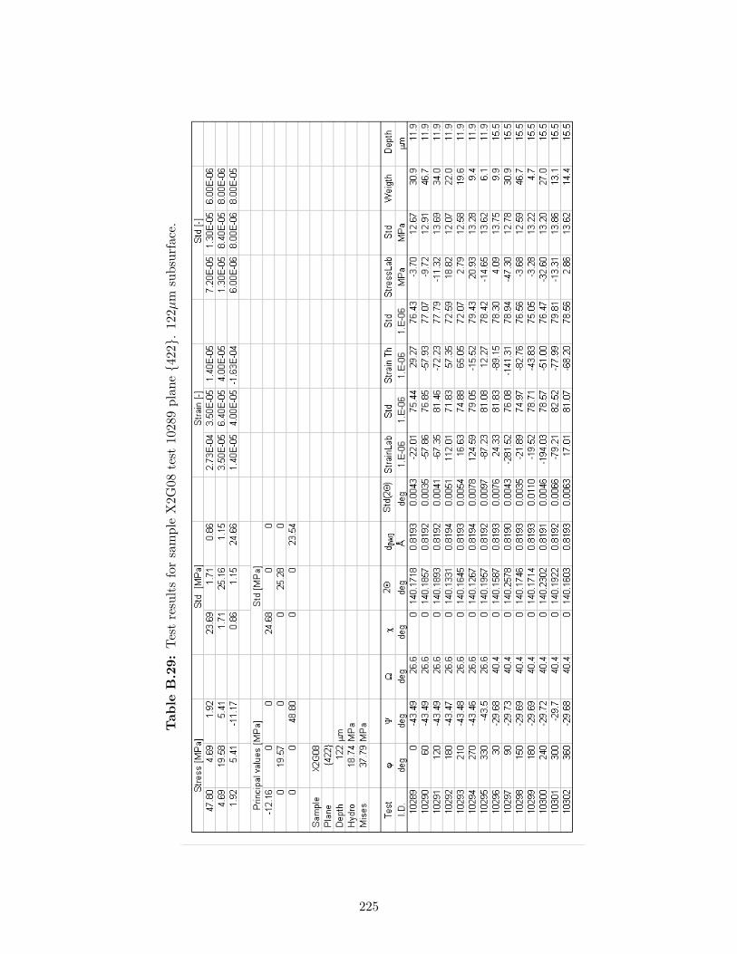
Tab
leB
.29:
Tes
tre
sult
sfo
rsa
mpl
eX
2G08
test
1028
9pl
ane4
22.
122µ
msu
bsur
face
.
225
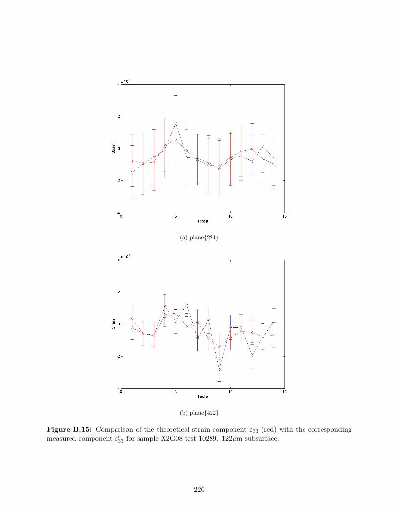
(a) plane224
(b) plane422
Figure B.15: Comparison of the theoretical strain component ε33 (red) with the correspondingmeasured component ε′33 for sample X2G08 test 10289. 122µm subsurface.
226
REFERENCES
Abaqus. Abaqus Explicit User’s manual, volume I. Hibbit, Karlsson, & Sorensen, INC., 2001. 8
Appel, F. and Wagner, R. “Microstructure and deformation of two-phase gamma-titaniumaluminides”. Materials Science and Engineering: R: Reports, 22(5):187–268, 1998. 1.2.3, 1.5
Asaro, R. “Crystal plasticity”. Transactions of the ASME. Journal of Applied Mechanics, 50(4B):921–934, 1983a. 8.2
Asaro, R. “Micromechanics of crystals and polycrystals”. Advances in Applied Mechanics, 23:1–115, 1983b. 8.2
Aurora, A., Marshall, D., Lawn, B., and Swain, M. “Indentation deformation/fracture ofnormal and anomalous glasses”. Journal of Non-Crystalline Solids, 31(3):415–428, 1979. 2.1, 7,7.1, 7.1, 7.5, 9.2, 9.4.5, 10.1.4
Austin, C., Kelly, T., McAllister, K., and Chesnutt, J. “Aircraft engine applications forgamma titanium aluminides”. In Proceedings of the Second International Symposium on Struc-tural Intermetallics, pages 413–425. The Minerals, Metals & Materials Soc (TMS), Warrendale,PA, USA, 1997. 1.1
Badger, J. and Torrance, A. “A comparison of two models to predict grinding forces fromwheel surface topography”. International Journal of Machine Tools and Manufacture, 40(8):1099–1120, 2000. 1.3
Balart, M., Bouzina, A., Edwards, L., and Fitzpatrick, M. “The onset of tensile residualstresses in grinding of hardened steels”. Materials Science and Engineering A, 367(1-2):132–142,2004. 1.4
Begley, M. and Hutchinson, J. “The mechanics of size-dependent indentation”. Journal of theMechanics and Physics of Solids, 46(10):2049–2068, 1998. 1.3
Behnken, H. and Hauk, V. “Determination of steep stress gradients by x-ray diffraction – resultsof a joint investigation”. Materials Science and Engineering A, 300(1-2):41–51, 2001. 6.6, 10.2
Bentley, S., Goh, N., and Aspinwall, D. “Reciprocating surface grinding of a gamma titaniumaluminide intermetallic alloy”. Journal of Materials Processing Technology, 118(1-3):22–28, 2001.1.4, 2.1
Bentley, S., Mantle, A., and Aspinwall, D. “The effect of machining on the fatigue strengthof a gamma titanium aluminide intertmetallic alloy”. Intermetallics, 7(8):967–969, 1999. 1.4,1.5.1, 2.1, 4.1
Blunt, L. and Ebdon, S. “The application of three-dimensional surface measurement techniquesto characterizing grinding wheel topography”. International Journal of Machine Tools and Man-ufacture, 36(11):1207–1226, 1996. 7.3
Bowden, F. and Tabor, D. The friction and lubrication of solids. Oxford University Press, 1950.7.1
227
Brady, M., Brindley, W., Smialek, J., and Locci, I. “Oxidation and protection of gammatitanium aluminides”. JOM, 48(11):46–50, 1996. 1.2
Brinksmeier, E. “State-of-the-art of non-destructive measurement of sub-surface material prop-erties and damages”. Precision Engineering, 11(4):211–224, 1989. 1.5
Briscoe, B., Biswas, S., and Panesar, S. “Scratch hardness and friction of a soft rigid-plasticsolid”. Wear of Materials: International Conference on Wear of Materials, 1:451–456, 1991. 1.3
Brockman, R. “Analysis of elastic-plastic deformation in tial polycrystals”. International Journalof Plasticity, 19(10):1749–1772, 2003. 2.3, 3.2
Butler, D., Blunt, L., See, B., Webster, J., and Stout, K. “The characterisation of grindingwheels using 3d surface measurement techniques”. Journal of Materials Processing Technology,127(2):234–237, 2002. 7.3
Cao, G., Fu, L., Lin, J., Zhang, Y., and Chen, C. “The relationships of microstructure andproperties of a fully lamellar tial alloy”. Intermetallics, 8(5-6):647–653, 2000. 1.2.2
Chatterjee, A., Dehm, G., Scheu, C., and Clemens, H. “Onset of microstructural instabilityin a fully lamellar ti-46.5 at.% al-4 at.% (cr,nb,ta,b) alloy during short-term creep”. Zeitschriftfuer Metallkunde/Materials Research and Advanced Techniques, 91(9):755–760, 2000. 1.2
Chen, X., Rowe, W., and Cai, R. “Precision grinding using cbn wheels”. International Journalof Machine Tools and Manufacture, 42(5):585–593, 2002. 1.7
Clemens, H. and Kestler, H. “Processing and applications of intermetallic gamma-tial-basedalloys”. Advanced Engineering Materials, 2(9):551–570, 2000. 1.2, 1.2.2
Clemens, H., Lorich, A., Eberhardt, N., Glatz, W., Knabl, W., and Kestler, H. “Tech-nology, properties and applications of intermetallic gamma-tial based alloys”. Zeitschrift furMetallkunde, 90(8):569–580, 1999. 1.2
Cuitio, A. and Ortiz, M. “Computational modeling of single crystals”. Modeling and Simulationin Materials Science and Engineering, 1(3):225–263, 1992. 8.2
Darolia, R. and Walston, W. “Effect of specimen surface preparation on room temperaturetensile ductility of an fe-containing nial single crystal alloy”. Intermetallics, 4(7):505–516, 1996.1.4
Dimiduk, D., Miracle, D., and Ward, C. “Development of intermetallic materials for aerospacesystems”. Materials Science and Technology, 8:367–375, 1992. 1.1
Dimiduk, D., Parthasarathy, T., and Hazzledine, P. “Design-tool representations of straincompatibility and stress-strain relationships for lamellar gamma titanium aluminides”. Inter-metallics, 9(10-11):875–882, 2001. 2.3
Dolle, H. and Hauk, V. “X-ray stress evaluation of residual stress systems having generalorientation”. Harterei-Techn. Mitt., 31:165, 1976. 6.4, 6.6
Dolle, H. and Hauk, V. “System for possible lattice strain distributions for mechanically stressedmetallic materials”. Zeitschrift fur metallkunde, 68(11):725–728, 1977. 6.4, 6.6
228
Ebbrell, S., Woolley, N., Tridimas, Y., Allanson, D., and Rowe, W. “The effects ofcutting fluid application methods on the grinding process”. International Journal of MachineTools and Manufacture, 40(2):209–223, 2000. 5.4.3
Eda, H., Kishi, K., and Ueno, H. “Cracking and fracture of matrix structure and carbideparticles produced by the grinding process”. Precision Engineering, 5(2):73–76, 1983. 1.4
Ely, T., Predecki, P., and Noyan, I. “A method for obtaining stress-depth profiles by absorp-tion constrained profile fitting of diffraction peaks”. Advances in X-Ray Analysis, 43, 1999. 6.3,6.6, 10.2
Engineer, F., Guo, C., and Malkin, S. “Experimental measurement of fluid flow through thegrinding zone”. Journal of Engineering for Industry, Transactions of the ASME, 114(1):61–66,1992. 5.4.3
Feng, C., Michel, D., and Crowe, C. “Twinning in tial”. Scripta Metallurgica, 23(7):1135–1140,1989. 1.2.1
Field, M. “Surface integrity in grinding”. In Shaw, M., editor, Proceedings of the Int. GrindingConference, New Developments in Grinding, Pittsburgh, PN, 1972. Carnegie Press. 1.4, 1.8
Field, M., Kahles, J., and Cammett, J. “A review of measuring methods for surface integrity”.Annals of CIRP, 21(2):219–238, 1972. 1.5, 1.5.1, 4.1
Forman, P. “Zygo interferometer system”. In Proceedings of the SPIE 192, 1979. 2.1, 4.3
Frank, G., Olson, S., and Brockman, R. “Numerical models of orthotropic and lamellar grainstructures”. Intermetallics, 11(4):331–340, 2003. 3.2
Furutani, K., Ohguro, N., Nguyen, T., and Nakamura, T. “In-process measurement oftopography change of grinding wheel by using hydrodynamic pressure”. International Journalof Machine Tools and Manufacture, 42(13):1447–1453, 2002. 5.4.4
Furutani, K., Ohguro, N., Nguyen, T., and Nakamura, T. “Automatic compensation forgrinding wheel wear by pressure based in-process measurement in wet grinding”. PrecisionEngineering, 27(1):9–13, 2003. 5.4.4
GE. “Diamond characterization”. Technical Report GES 1278 E, 2000. 5.3
Gillespie, L. Deburring and edge finishing handbook. 1977. 4.1
Goh, C. Crystallographic Plasticity in Fretting of Ti-6Al-4V. Doctoral dissertation, GeorgiaInstitute of Technology, 2003. 8.3.2
Grum, J. “A review of the influence of grinding conditions on resulting residual stresses afterinduction surface hardening and grinding”. Journal of Materials Processing Technology, 114(3):212–226, 2001. 1.4
Guo, C. and Malkin, S. “Analysis of fluid flow through the grinding zone”. Journal of Engineeringfor Industry, Transactions of the ASME, 114(4):427–434, 1992. 5.4.3
Hahn, R. and Lindsay, R. “Principles of grinding. part i: Basic relationships in precision ma-chining”. In Bhateja, C. and Lindsay, R., editors, Grinding Theory Techniques and Trou-bleshooting. SME, 1982a. 1.1, 7.1
229
Hahn, R. and Lindsay, R. “Principles of grinding. part ii: The metal removal parameter”. InBhateja, C. and Lindsay, R., editors, Grinding Theory Techniques and Troubleshooting, pages11–17. SME, 1982b. 1.1, 7.1
Hahn, R. and Lindsay, R. “Principles of grinding. part iii: The wheel removal parameter”. InBhateja, C. and Lindsay, R., editors, Grinding Theory Techniques and Trouble Shooting, page1824. SME, 1982c. 1.1
Hahn, R. and Lindsay, R. “Principles of grinding. part iv: Surface finish, geometry, and in-tegrity”. In Bhateja, C. and Lindsay, R., editors, Grinding Theory Techniques and TroubleShooting. SME, 1982d. 1.1
Hall, E. and Huang, S.-C. “Deformation mechanisms in gamma titanium aluminides. a re-view”. In Proceedings of the Symposium of Microstructure-Properties Relationship for TitaniumAluminides Alloys, pages 47–64. The Minerals, Metals & Materials Soc (TMS), Warrendale, PA,USA, 1991. 1.2.2
Hao, Y., Xu, D., Cui, Y., Yang, R., and Li, D. “The site occupancies of alloying elements intial and ti3al alloys”. Acta Materialia, 47(4):1129–1139, 1999. 1.2.2, 3.1
Hecker, R. Part surface roughness modeling and process optimal control of cylindrical grinding.Doctoral dissertation, Georgia Institute of Technology, 2002. 2.3, 7, 7.1, 7.1, 7.3
Hono, K., Abe, E., Kumagai, T., and Harada, H. “Chemical compositions of ultrafine lamellaein the water-quenched ti− 48al alloy”. Scripta Materialia, 35(4):495–499, 1996. 1.2.2, 1.3
Hutchings, I. Tribology. CRC Press, 1992. 1.3
Hwang, T., Evans, C., and Malkin, S. “Size effect for specific energy in grinding of siliconnitride”. Wear, 225-229(Part 2):862–867, 1999. 1.3
Inui, H., Nakamura, A., Oh, M., and Yamaguchi, M. “Deformation structures in ti-rich tialpolysynthetically twinned crystals”. Philosophical Magazine A (Physics of Condensed Matter,Defects and Mechanical Properties), 66(4):557–573, 1992a. 1.2.3
Inui, H., Oh, M., Nakamura, A., and Yamaguchi, M. “Ordered domains in tial coexisting withti3al in the lamellar structure of ti-rich tial compounds”. Philosophical Magazine A (Physics ofCondensed Matter, Defects and Mechanical Properties), 66(4):539–555, 1992b. 1.2.1
Jones, P. Effects of conventional machining on high cycle fatigue behavior of the intermetallicalloy Ti − 47Al − 2Nb − 2Cr (at.%). Doctoral dissertation, University of Dayton, 1997. 2.1,9.4.1, 9.4.2, 9.4, 9.5
Jones, P. and Eylon, D. “Effects of conventional machining on high cycle fatigue behavior ofthe intermetallic alloy ti− 47al − 2nb− 2cr (at.%)”. Materials Science and Engineering A, 263(2):296–304, 1999. 1.4, 1.5.1, 2.1, 4.1, 9.4.2
Kad, B., Dao, M., and Asaro, R. “Numerical simulations of stress-strain behavior in two-phaseα2 + γ lamellar tial alloys”. Materials Science and Engineering A, 192-193(Part 1):97–103, 1995.2.3, 8.2, 8.3.2
Kagiwada, T. and Kanauchi, T. “Three-dimensional thermal deformation and thermal stressin workpieces under surface grinding”. Journal of Thermal Stresses, 8(3):305–318, 1985. 1.4
230
Kattner, U., Lin, J.-C., and Chang, Y. “Thermodynamic assessment and calculation of theti-al system”. Metallurgical Transactions A (Physical Metallurgy and Materials Science), 23A(8):2081–2090, 1992. 1.2.1, 1.1, 1.2.2, 3.1
Kawabata, T., Tamura, T., and Izumi, O. “Parameters for ductility improvement in tial”.In Liu, C., editor, High Temperature Ordered Intermetallic Alloys III, pages 329–334. MRS,Pittsburgh, PA, 1989. 1.2.2, 3.1
Kim, H., Theodore, N., Gadre, K., Mayer, J., and Alford, T. “Investigation of thermalstability, phase formation, electrical, and microstructural properties of sputter-deposited titaniumaluminide thin films”. Thin Solid Films, 460(1-2):17–24, 2004. 1.2
Kim, Y.-W. “Intermetallic alloys based on gamma titanium aluminide”. JOM, 41(7):24–30, 1989.1.2, 1.2.2
Kim, Y.-W. “Ordered intermetallic alloys. part iii: gamma titanium aluminides”. Journal ofMetals, 46(7):30–39, 1994. 1.2.2
Kim, Y.-W. “Trends in the development of γ − tial alloys”. In Gamma Titanium Aluminides I.The Minerals, Metals & Materials Soc (TMS), Warrendale, PA, USA, 1995. 1.1
Kim, Y.-W. and Dimiduk, D. “Progress in the understanding of gamma titanium aluminides”.JOM, 43(8):40–47, 1991. 1.2
Knippscheer, S. and Frommeyer, G. “Intermetallic tial(cr,mo,si) alloys for lightweight engineparts. structure, properties, and applications”. Advanced Engineering Materials, 1(3-4):187–191,1999. 1.2
Kondoh, T., Goto, T., Sasaki, T., and Hirose, Y. “X-ray stress measurement for titaniumaluminide intermetallic compound.”. Advances in X-Ray Analysis, 43, 1999. 1.4
Konig, W. and Lortz, W. “Properties of cutting edges related to chip formation in grinding”.Annals of CIRP, 24(1):231–235, 1975. 7.2
Kumar, K. “Superabrasive grinding of titanium alloys. paper mr90-505”. In 4th InternationalGrinding Conference, Dearborn, Michigan, 1990. 5.3
Kumar, K. “Superabrasive grinding of aerospace materials, diamond & cbn ultrahard materials”.In Symposium ’93, Windson, Ontario, Canada, 1993. 5.3
Larsen, J., Worth, B., Balsone, S., and Rosenberger, A. “Reliability issues affecting theimplementation of gamma titanium aluminides in turbine engine applications”. In Blenkinsop,P., Evans, W., and Flower, H., editors, Titanium 95, volume 1, page 113120. The Instituteof Materials, London, UK, 1996. 1.1
Lawn, B. and Wilshaw, T. “Indentation fracture: Principles and applications”. Journal ofMaterials Science, 10:1049–1081, 1975. 2.1, 7, 7.1, 7.1, 7.5, 9.2, 9.4.5, 10.1.4
Lee, E. “Elastic-plastic deformation at finite strains”. Journal of Applied Mechanics, 36:1–6, 1969.8.2
Liu, Z., Sun, J., and Shen, W. “Study of plowing and friction at the surfaces of plastic deformedmetals”. Tribology International, 35(8):511–522, 2002. 1.5.1
231
Ludema, K. “Mechanism-based modeling of friction and wear”. Wear, 200(1-2):1–7, 1996. 1.3
Mahdi, M. and Zhang, L. “Applied mechanics in grinding–v. thermal residual stresses”. Inter-national Journal of Machine Tools and Manufacture, 37(5):619–633, 1997. 1.4
Malkin, S. Grinding Technology. Theory and Applications of Machining with Abrasives. EllisHorwood Limited, New York, 1989. 1.1, 7.4.1
Mantle, A. and Aspinwall, D. “Surface integrity of a high speed milled gamma titaniumaluminide”. Journal of Materials Processing Technology, 118(1-3):143–150, 2001. 2.1
Marketz, W., Fischer, F., and Clemens, H. “Deformation mechanisms in tial intermetallics–experiments and modeling”. International Journal of Plasticity, 19(3):281–321, 2003. 1.2.2
Matsuno, Y., Yamada, H., Harada, M., and Kobayashi, A. “Microtopography of the grindingwheel surface with sem”. Annals of CIRP, 24(1):237–242, 1975. 7.3
McGinty, R. Multiscale Representation of Polycrystalline Inelasticity. Doctoral dissertation,Georgia Institute of Technology, 2001. 2.3, 8.2
McGinty, R. and McDowell, D. “Multiscale polycrystal plasticity”. Journal of EngineeringMaterials and Technology, 121:203–209, 1999. 8.2
McQuay, P., Simpkins, R., Seo, D., and Bieler, T. “Alloy and process improvements forcast gamma tial alloy applications”. In Kim, Y.-W., Dimiduk, D., and Loretto, M., editors,Gamma Titanium Aluminides, pages 197–207. The Minerals, Metals & Materials Soc (TMS),Warrendale, PA, USA, 1999. 1.2.2, 3.1
Meng, H. and Ludema, K. “Wear models and predictive equations: their form and content”.Wear, 181-183(2):443–457, 1995. 1.3, 9.1
Nakayama, K., Brecker, J., and Shaw, M. “Grinding wheel elasticity”. Journal of Engineeringfor Industry, Transactions of the ASME, 93:609, 1971. 7.2
Nelson, L. Subsurface damage in the abrasive machining of Titanium Aluminide. PhD thesis,Georgia Institute of Technology, 1997. 1.5.1, 2.1, 2.3, 4.2, 7, 7.1, 7.1, 9.2, 9.4.4
Newby, J. ASM Handbook: Mechanical Testing, volume 8. American Society of Metals Interna-tional, 1989. 1.5.1
Noda, T., Okabe, M., Isobe, S., and Sayashi, M. “Silicide precipitation strengthened tial”.Materials Science and Engineering A, 192-193(Part 2):774–779, 1995. 1.2.2
Novovic, D., Dewes, R., Aspinwall, D., Voice, W., and Bowen, P. “The effect of ma-chined topography and integrity on fatigue life”. International Journal of Machine Tools andManufacture, 44(2-3):125–134, 2004. 1.4, 2.1
Noyan, I. and Cohen, J. Residual stress, measurement by diffraction and interpretation. Springer-Verlag, New York, 1987. 6.3
Ohmori, H., Takahashi, I., and Bandyopadhyay, B. P. “Ultra-precision grinding of structuralceramics by electrolytic in-process dressing (elid) grinding”. Journal of Materials ProcessingTechnology, 57(3-4):272–277, 1996. 5.4.1
232
Ohnuma, I., Fujita, Y., Mitsui, H., Ishikawa, K., Kainuma, R., and Ishida, K. “Phaseequilibria in the ti-al binary system”. Acta Materialia, 48(12):3113–3123, 2000. 1.2.1, 1.1, 3.1
Pagano, N. “Exact moduli of anisotropic laminates”. In Sendeckyj, G., editor, Mechanics ofcomposite materials. Academic Press, New York, 1974. 3.2
Perez, P., Jimenez, J., Frommeyer, G., and Adeva, P. “Oxidation behaviour of a ti-46al-1mo-0.2si alloy: the effect of mo addition and alloy microstructure”. Materials Science andEngineering A, 284(1-2):138–147, 2000. 1.2.2
Razavi, H. Identification and Control of Grinding Processes for Intermetalic [sic] Compunds [sic].Doctoral dissertation, Georgia Institute of Technology, 2000. 1.5.1, 2.1, 4.2, 7, 7.1, 9.2
Razavi, H., Kurfess, T., and Danyluk, S. “Force control grinding of gamma titanium alu-minide”. International Journal of Machine Tools and Manufacture, 43:185–191, 2003. 4.2
Richter, H. and Hofmann, F. “Residual stress measurements on machined specimens of gammatitanium aluminine material.”. Mat.-wiss. u. Werkstofftech, 33:24–32, 2002. 1.4, 2.3
Robinson, P. and Bradbury, S. Qualitative Polarized-Light Microscopy. Royal MicroscopySociety, Oxford University Press, Oxford, 1992. 1.5.1, 4.1
Rowe, W., Morgan, M., Qi, H., and Zheng, H. “The effect of deformation on the contact areain grinding”. Annals of CIRP, 42(1):409–412, 1993. 7.2
Schneibel, J., Agnew, S., and Carmichael, C. “Surface preparation and bend ductility ofnial”. Metallurgical Transactions A (Physical Metallurgy and Materials Science), 24A(11):2593–2596, 1993. 1.4
Seo, D., Saari, H., Beddoes, J., and Zhao, L. “The creep behaviour of tial+w as a functionof the fully lamellar morphology”. In Hemker, K., Dimiduk, D., Clemens, H., Darolia, R.,Inui, H., Larsen, J., Sikka, V., Thomas, M., and Whittenberger, J., editors, StructuralIntermetallics 2001, pages 653–662. TMS Warrendale, PA, USA, 2001. 1.2.2
Sharman, A., Aspinwall, D., Dewes, R., and Bowen, P. “Workpiece surface integrity con-siderations when finish turning gamma titanium aluminide”. Wear, 249(5-6):473–481, 2001a.2.1
Sharman, A., Aspinwall, D., Dewes, R., Clifton, D., and Bowen, P. “The effects ofmachined workpiece surface integrity on the fatigue life of gamma-titanium aluminide”. Inter-national Journal of Machine Tools and Manufacture, 41(11):1681–1685, 2001b. 1.4, 2.1
Shaw, M. New Developments in Grinding. Carnegie Press, 1972. 1.1, 1.3, 1.3, 7.3
Shemet, V., Yurechko, M., Tyagi, A., Quadakkers, W., and Singheiser, L. “The influenceof nb and zr additions on the high temperature oxidation mechanisms of tial alloys in ar/o2”. InKim, Y.-W., Dimiduk, D., and Loretto, M., editors, Gamma Titanium Aluminides, pages783–790. The Minerals, Metals & Materials Soc (TMS), Warrendale, PA, 1999. 1.2.2, 3.1
Stone, W. Thermal effects on subsurface damage during the surface grinding of Titanium Alu-minide. Doctoral dissertation, Georgia Institute of Technology, 2003. 1.5.1, 2.1, 4.2, 7, 7.1,9.2
233
Subhash, G., Koeppel, B., and Chandra, A. “Dynamic indentation hardness and rate sensi-tivity in metals”. Journal of Engineering Materials and Technology, 121(3):257–263, 1999. 1.3
Suominen, L. and Carr, D. “Selected methods of evaluating residual stress gradients measuredby x-ray diffraction. traditional, full tensor, and wavelet.”. Advances in X-Ray Analysis, 43:21–30, 1999. 6.6, 10.2
Tetsui, T. “Effects of high niobium addition on the mechanical properties and high-temperaturedeformability of gamma tial alloy”. Intermetallics, 10(3):239–245, 2002. 1.2.2, 3.1
Tlusty, G. Manufacturing Process and Equipment. Prentice Hall, 1999. 1.3, 1.3
Trail, S. and Bowen, P. “Effects of stress concentrations on the fatigue life of a gamma-basedtitanium aluminide”. Materials Science and Engineering A, 192-193(Part 1):427–434, 1995. 1.4,2.1
Umakoshi, Y., Nakano, T., Sumimoto, K., and Maeda, Y. “Plastic anisotropy of ti3al singlecrystals”. Materials Research Society Symposium Proceedings, 288:441–446, 1993. 1.2.3
Underwood, E. Quantitative stereology. Addison-Wesley Publishing Company, 1970. 7.3
Verkerk, J. and Peters, J. “Final report concerning cirp cooperative work on the characteri-zation of grinding wheel topography”. Annals of CIRP, 26(2):385–395, 1977. 1.3, 7.2
Viswanathan, G., Kim, Y.-W., and Mills, M. “On the role of precipitation strengthening inlamellar ti-46al alloy with c and si addition”. In Kim, Y.-W., Dimiduk, D., and Loretto, M.,editors, Gamma Titanium Aluminides 1999, pages 653–660. TMS, Warrendale, PA, 1999. 1.2.2
Wagner, C., Boldrick, M., and Perez-Mendez, V. “A phi-psi-diffractometer for residualstress measurements”. Advances in X-Ray Analysis, 26:275–282, 1983. 2.3
Wang, H. and Subhash, G. “Mechanics of mixed-mode ductile material removal with a conicaltool and the size dependence of the specific energy”. Journal of the Mechanics and Physics ofSolids, 50(6):1269–1296, 2002. 1.3, 1.3
Wern, H. “Evaluation of residual stress gradients by diffraction methods with wavelets; a neuralnetwork approach.”. Advances in X-Ray Analysis, 43:11–20, 1999. 6.6, 10.2
Williams, J. “Wear modelling: analytical, computational and mapping: a continuum mechanicsapproach”. Wear, 225-229(Part 1):1–17, 1999. 1.3
Winholtz, R. and Cohen, J. “Generalized least-squares determination of triaxial stress states byx-ray diffraction and the associated errors”. Australian Journal of Applied Physics, 41:189–99,1988. 2.3, 6.4, 6.6
Woodbury, R. History of the Grinding Machine. 1959. 1.1
Xu, H. and Jahanmir, S. “Simple technique for observing subsurface damage in machiningceramics”. Journal of American Ceramics Society, 77(5):1388–1390, 1994. 1.5.1, 2.3, 4.2
Yamabe, Y., Takeyama, M., and Kikuchi, M. “Determination of α (a3) → α2 (d019) transitiontemperatures in ti-(40 45)at.%al alloys”. Scripta Metallurgica et Materialia, 30(5):553–557,1994. T. 1.2.1, 3.2
234
Yamabe, Y., Takeyama, M., and Kikuchi, M. “Microstructure evolution through solid-solidphase transformation in gamma titanium aluminides”. In Proceedings of the Symposium onTMS Annual Meeting on Gamma Titanium Aluminides, pages 111–129. The Minerals, Metals &Materials Soc (TMS), Warrendale, PA, USA, 1995. 1.2.2
Yamaguchi, M. and Inui, H. “Tial compounds for structural applications”. pages 127–142, 1993.1.2.1
Yamaguchi, M., Inui, H., and Ito, K. “High-temperature structural intermetallics”. ActaMaterialia, 48(1):307–322, 2000. 1.2.1
Yamaguchi, M. and Umakoshi, Y. “The deformation behaviour of intermetallic superlatticecompounds”. Progress in Materials Science, 34(1):1–148, 1990. 1.2.2, 1.2.3
Yoo, M. and Fu, C. “Physical constants, deformation twinning, and microcracking of titaniumaluminides”. Metallurgical and Materials Transactions A: Physical Metallurgy and MaterialsScience, 29A(1):49–63, 1998. 3.2
Younis, M. and Alawi, H. “Probabilistic analysis of the surface grinding process”. Transactionsof the CSME, 8(4):208–213, 1984. 7.2
Zhang, W.-J., Lorenz, U., and Appel, F. “Recovery, recrystallization and phase transforma-tions during thermomechanical processing and treatment of tial-based alloys”. Acta Materialia,48(11):2803–2813, 2000. 1.2.2
Zhang, W. and Deevi, S. “An analysis of the lamellar transformation in tial alloys containingboron”. Materials Science and Engineering A, 337(1-2):17–20, 2002. 1.2.2, 3.1
Zhu, X., Ballard, B., and Predecki, P. “Determination of z-profiles of diffraction data fromtau- profiles using a numerical linear inversion method,”. Advances in X-Ray Analysis, 38, 1995.6.6, 10.2
235
VITA
Gregorio Murtagian is a graduate from Escuelas Tecnicas Municipales Raggio (Argentina) high
school, and he received his Mechanical Engineering Degree at Universidad Technological Nacional,
Facultad Regional Buenos Aires in 1994. He completed a Materials Science and Technology Master’s
in 1997 working in the area of dynamic fracture. During the period of 1995-1999 he worked as a
researcher at the Center for Industrial Research CINI-TENARIS. He started his PhD program at
Georgia Institute of Technology on Fall 1999.
236
Related Documents


![BOOK OF ABSTRACTS · 2007. 3. 16. · [C088] Gamma Titanium Aluminide Matrix Composites: A Parametric Study of Optimum Constituents 83 J.S. Craft and W. S. Johnson [C001] The Effect](https://static.cupdf.com/doc/110x72/606b3af84a82022923479c71/book-of-2007-3-16-c088-gamma-titanium-aluminide-matrix-composites-a-parametric.jpg)