Surface Impedance Mapping Using Sferics

This article has been accepted for inclusion in a future issue of this journal. Content is final as presented, with the exception of pagination.

IEEE TRANSACTIONS ON GEOSCIENCE AND REMOTE SENSING 1

Surface Impedance Mapping Using SfericsGavin T. Mogensen, Hugo G. Espinosa, and David V. Thiel, Senior Member, IEEE

Abstract— Naturally occurring radio emissions from discretesferics in the frequency range 500 Hz to 30 kHz have the potentialfor shallow conductivity profiling beneath the surface of theearth. A dual-channel time-domain receiver was constructed andused over selected geophysical targets. The instrumentation wasvalidated through a comparison with very low-frequency surfaceimpedance measurements from a distant navigation transmitterand 2-D modeling using the impedance method. The multifre-quency results were then verified using this 2-D modeling. Theskin effect shows the frequency dependence of electromagneticfield strength dissipation as a signal enters a multilayered earth.Single-frequency methods offer fixed depth conductivity profileswhereas multiple frequencies reveal multiple depth conductivityprofiles that can help with 3-D modeling of subsurface featuresand anomalies. Several electromagnetic techniques offer multiple-frequency operation capitalizing upon this effect however thesetechniques generally use a local artificial signal source, whichleads to near-field distortion effects in the measured data.This method shows significant promise for cost-effective, high-speed, ground-level surface impedance measurements targetingsubsurface features down to 100 m.

Index Terms— Impedance method, sferics, subsurfacemapping, surface impedance.

I. INTRODUCTION

SURFACE impedance measurements—initially referred toas the magnetotelluric method—have been used for many

decades to map subsurface features of the earth [1]–[3].Very low-frequency (VLF) electromagnetic fields in the upperatmosphere drive currents in the earth, which can be measuredat the surface of the earth using wire and loop probes [4].The driving fields can be the result of distant lighting strikes,communications and navigation transmitters, and currents inthe ionosphere. For a single frequency, surface impedancemeasurements are used in subsurface probing of the earth todepths of up to 100 m [5]. These measurements rely on VLFradio navigation transmitters around the world that transmitvertically polarized signals. For multifrequency recordings, theelectric and magnetic fields of atmospheric transients (alsoknown as sferics) can be used for surface impedance mea-surements [6], [7]. Of particular interest are sferics generatedin the far field—these are signals that have a source locationat distances >500 km away [8]. Sferics contain significantenergy in the frequency band of 500 Hz to 30 kHz [9].

Manuscript received October 22, 2012; revised February 4, 2013, April 1,2013; accepted April 2, 2013. This work was supported in part by AustralianPostgraduate Scholarship and GeoConsult Pty Ltd - Geophysical Services.

The authors are with the Centre for Wireless Monitoring andApplications, Griffith University, Brisbane 4111, Australia (e-mail:[email protected]; [email protected]; [email protected]).

Color versions of one or more of the figures in this paper are availableonline at http://ieeexplore.ieee.org.

Digital Object Identifier 10.1109/TGRS.2013.2257801

The TSIM device is a dual-channel VLF receiver thatmonitors narrow band signals, which has been used in theAustralian open cut coal fields since 1983 [10]. The unitdetects the horizontal electric field Ex using a 10-m asymmet-ric insulated dipole wire antenna lying on the surface of theearth, the horizontal magnetic field Hy using a shielded ferritecored, multiturn loop antenna, and the phase between them.The surface impedance Zs is a complex number determinedby the ratio of both fields Ex and Hy, where the phasedifference is the argument of Zs . The newer TranSIM deviceis also dual-channel VLF receiver, which detects broadbandtransient signals in the 500 Hz to 30 kHz frequency range.In this paper, the TranSIM instrumentation is validated forsingle-frequency operation, through a comparison with a ThielSurface Impedance Meter (TSIM) [4], [5]. Multifrequencyvalidation is performed through a comparison with the com-putational electromagnetic impedance method [11], [12].

Single-frequency methods offer only a limited depth profileas dictated by the skin depth effect. The use of multiplefrequencies allows for investigation at different depths andprovides extra depth conductivity information that can helpimprove subsurface feature and anomaly identification. Betterdepth conductivity profiles can also benefit 3-D inversionmodels by supplying more detailed input data.Various electro-magnetic techniques offer multiple-frequency operation capi-talizing upon the skin effect, such as controlled source audiomagnetotellurics (CSAMT) and time-domain electromagnetics(TDEM). These methods use the artificial signal sources thatare commonly high powered and expensive. The logistics oftransporting expensive heavy equipment to remote survey sitescan be prohibitive, whereas the TranSIM device is a single-operator handheld unit that allows ease of access to manydifficult access survey sites. More importantly, each of theabove methods suffers measurement distortions because of thenear-field effects of the source signal. These distortions are dueto wavetilt of the incident electromagnetic wave and results insome wave energy being reflected away rather than travelingdown through the earth layers. Far-field signals eliminate theseproblems and simplify calculations for apparent resistivity.

The impedance method was derived to solve quasi-staticelectromagnetic and radiation problems [11]. The solutionspace is discretized by dividing the object into cells andusing an impedance element at each edge of the cell torepresent both the size of the cell and the electromagneticproperties of the material enclosed. In the formulation ofthe method, the incident magnetic field is uniform and thecurrent in each impedance element is calculated via an efficienttechnique. Because of the dimensions of the problem for onefrequency, the model can be solved by a direct method. How-ever, for multifrequency modeling (1024 frequencies recorded

0196-2892/$31.00 © 2013 IEEE

This article has been accepted for inclusion in a future issue of this journal. Content is final as presented, with the exception of pagination.

2 IEEE TRANSACTIONS ON GEOSCIENCE AND REMOTE SENSING

by TranSIM), the algorithm must be run multiple times ateach frequency for in-field inversion. For that reason, aniterative solver together with a preconditioner is implementedto improve the speed, size, and convergence of the solution[12], [13].

This paper is organized as follows. The surface impedancetheory is briefly presented in Section II. The computationalmethod is described in Section III. The dual-channel time-domain receiver and the fast Fourier transform data processingare presented in Sections IV and V, respectively. Section VIpresents numerical results of experiments performed: 1) at asingle VLF frequency from a navigation transmitter and 2)at multiple frequencies. Finally, Section VII concludes andsummarizes the work.

II. SURFACE IMPEDANCE THEORY

The electromagnetic surface impedance of the earth isdefined as the ratio of the horizontal electric field componentEx in the direction of propagation to the horizontal magneticfield component Hy perpendicular to it [14]. For a uniformhalf-space, the surface impedance is dependent only upon theelectrical properties of the half-space and is given by

Zs = Ex

Hy=

√jωμ

σ + jεω(1)

where σ is the conductivity and ε is the permittivity. The sur-face impedance is a complex number, as the phase relationshipbetween the two fields components will vary. If the earth ishorizontally layered, then the surface impedance given by (1)is modified by a factor Q [14] defined as

Zs = QZ1 (2)

where Z1 is the intrinsic impedance of the upper layer. For atwo-layer earth

Q =Z2 + Z1 tanh

(h

√γ 2

1 − γ 20 sin2 φ

)

Z1 + Z2 tanh

(h

√γ 2

1 − γ 20 sin2 φ

) (3)

where Z2 is the surface impedance of the lower half-space, μ1is the complex propagation coefficient for the top layer in thevertical direction, γ0 is the free-space propagation coefficient,γ1 is the propagation coefficient in the first layer, η is the angleof incidence measured with respect to the surface normal, andh is the depth of the upper layer. The factor Q in (3) isdependent on the depth of the layer h and the conductivityof both media. The propagation coefficients are determinedby

φn = j√

ω2μnεn − jωμnσn (4)

where μn , εn , and σn are the permeability, permittivity, andconductivity of layer n, respectively. The surface impedancemeasurement from (1) is commonly expressed in terms of anapparent resistivity σa [3] defined by

ρa = |ZS|2ωμ

(5)

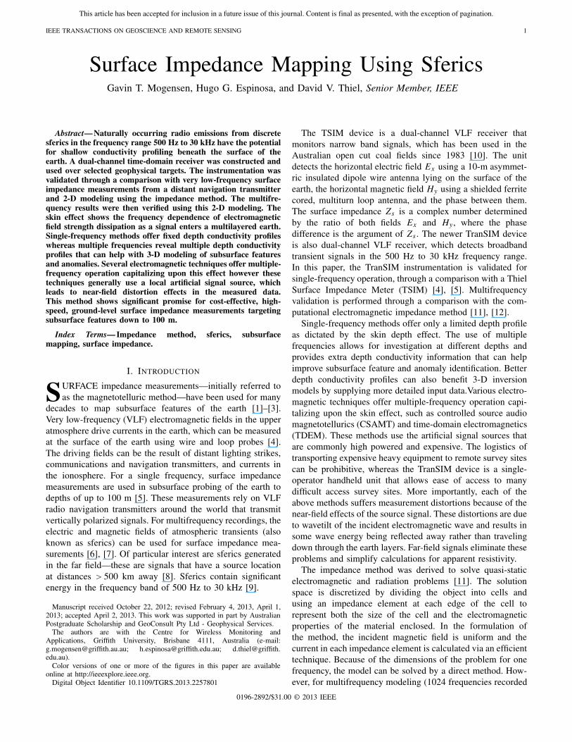
Fig. 1. Portion of a 2-D mesh with a cell bounded by impedance elements.

where ω is the angular frequency of the radiation and μ is themagnetic permeability of the earth.

III. IMPEDANCE METHOD

Surface-impedance measurements are used successfully tomap the conductivity structure of the upper parts of theearth’s subsurface; however, given its complexities includingdislocations, discontinuities, and folded structures, the forwardmodeling problem using the analytical method of Section I islimited to few idealized cases [15]. Therefore, the impedancemethod is implemented to analyze very large and complexproblems.

The impedance method requires the solution space to bedivided into 2-D rectangular cells bounded by impedanceelements with properties dependent on the local electromag-netic properties of the medium and the cell size. In theformulation, the magnetic field is assumed to be known atthe source and can be introduced at one or more locationsin the solution space [11]. Fig. 1 shows a portion of a2-D solution space divided into rectangular cells bounded byimpedance elements.

From Fig. 1, Ii,k is the circulating current in the (i, k)th celland can be determined in terms of the four adjacent cells. Theimpedance of the (i, k)th element can be defined as

Zmik = xi,k

(σik + jωεik)yZi,k(6)

where m = 1–4 impedance elements, σi,k and εi,k are theconductivity and permittivity, respectively, of the materiallocated in the (i, k)th cell, zi,k is the height of the firstelement, and y is a constant width assigned to all elementsthroughout the solution space required by the 2-D formu-lation and it is eliminated during the mathematical devel-opment. Using a combination of Ampere’s, Faraday’s, and

This article has been accepted for inclusion in a future issue of this journal. Content is final as presented, with the exception of pagination.

MOGENSEN et al.: SURFACE IMPEDANCE MAPPING 3

Kirchhoff’s laws, the magnetic field Hi,k , in each element,can be calculated using the matrix equation

[S]N×N [H]N×1 = [H0]N×1 (7)

where H is the vector of unknown magnetic field elements,H0 is the known source field vector (in general, the number ofnon-zero elements in H0 will be small), N is the number ofimpedance elements in the solution space matrix, and S is asparse (tridiagonal with two off-side bands), square, matrixof size N2, which, although dimensionless, represents theelectrical properties and the physical dimensions of the pixelsin the solution space. The solution matrix SN×N is given interms of the complex propagation coefficient γik in the (i, k)thwhich is defined as

γi,k = j√

ω2μikεik − jωμikσik. (8)

The linear system of (7) can be efficiently solved to findthe vector of magnetic field elements H by using the GMRESiterative solver together with the modified ILU preconditioneras described in [12] and [13]. Once the solution vector H from(7) is determined, the surface impedance Zs can be calculated.If the source field is set at the top of the solution space, andthe air/material interface is at the top of the (i, k)th cell, thenthe electromagnetic surface impedance can be written as

ZS = Ex

Hy= (Hi,k − Hi,k−1)

(σik + jωεik)Hi,k−1zi,k. (9)

IV. TRANSIENT SURFACE IMPEDANCE METER (TRANSIM)

The TranSIM device comprises a hand-held electronicinstrument with antennas for both the magnetic and electricfields. The horizontal E and H field signals are amplifiedand bandpass filtered before being simultaneously sampled byonboard 12-bit analog-to-digital converters. The recorded datais streamed to a host computer via wireless communications,where the apparent resistivity calculations are performed andpresented graphically to the user. The instrument is alsoequipped with onboard GPS hardware and high-speed wire-less communications allowing for data transfer between ahost computer or other TranSIM units. The instrumentationhas been designed to specifically target and record sfericenergy from the ionosphere and the induced fields at thesurface of the earth with a frequency range of 500 Hz to30 kHz [8], [9].

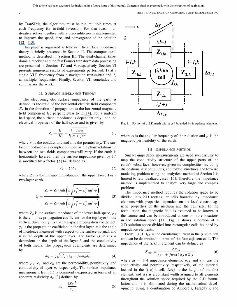
The primary magnetic field (H) is detected by a multiturncoil antenna located on the front of the device at ground leveland perpendicular to the signal source. The correspondinginduced electric field is measured using 10-m, insulated single-wire antenna, which is dragged along the ground behindthe device between sampling points. The signals from bothantennas are simultaneously sampled at a rate of 60 000samples per second, with each sample set comprising of 2048data points. Post-data processing and graphical representationsof apparent resistivity and phase relationships are displayed ona graphical user interface on the application software allowingfor immediate feedback to the operator. Fig. 2 shows theTranSIM instrumentation with a screenshot of the applicationsoftware for on-site data processing and graphical display.

Fig. 2. TranSIM instrumentation, showing circuit board and prototypehousing and brass H field antenna at the front.

Signal to noise ratios between both the TSIM and TranSIMare almost identical as measured by performing rotational teststo find maxima and minima at single frequency of 19.8 kHz.

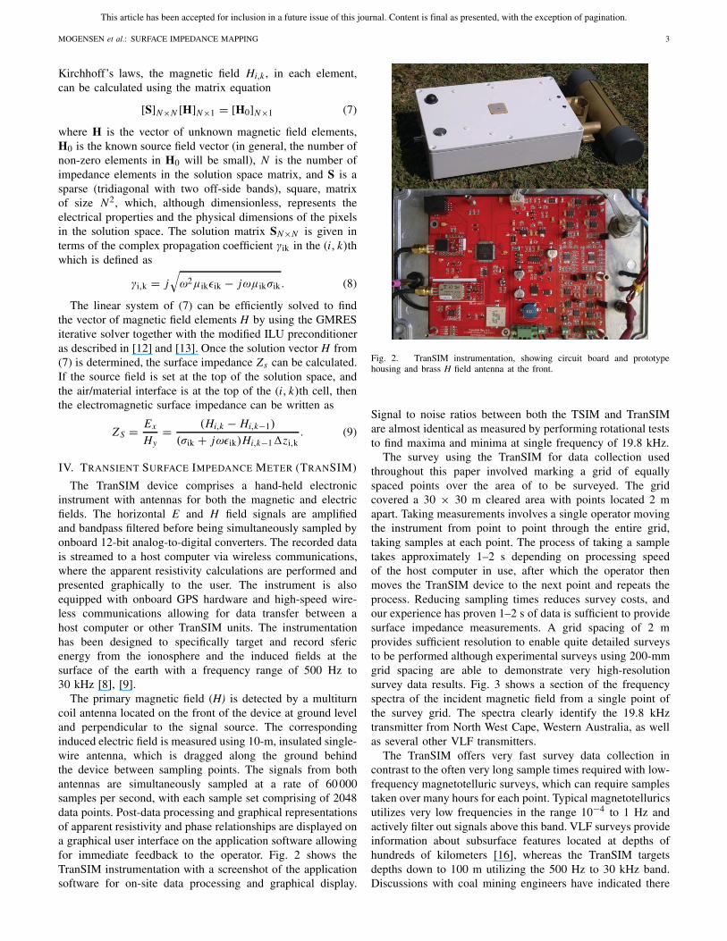
The survey using the TranSIM for data collection usedthroughout this paper involved marking a grid of equallyspaced points over the area of to be surveyed. The gridcovered a 30 × 30 m cleared area with points located 2 mapart. Taking measurements involves a single operator movingthe instrument from point to point through the entire grid,taking samples at each point. The process of taking a sampletakes approximately 1–2 s depending on processing speedof the host computer in use, after which the operator thenmoves the TranSIM device to the next point and repeats theprocess. Reducing sampling times reduces survey costs, andour experience has proven 1–2 s of data is sufficient to providesurface impedance measurements. A grid spacing of 2 mprovides sufficient resolution to enable quite detailed surveysto be performed although experimental surveys using 200-mmgrid spacing are able to demonstrate very high-resolutionsurvey data results. Fig. 3 shows a section of the frequencyspectra of the incident magnetic field from a single point ofthe survey grid. The spectra clearly identify the 19.8 kHztransmitter from North West Cape, Western Australia, as wellas several other VLF transmitters.

The TranSIM offers very fast survey data collection incontrast to the often very long sample times required with low-frequency magnetotelluric surveys, which can require samplestaken over many hours for each point. Typical magnetotelluricsutilizes very low frequencies in the range 10−4 to 1 Hz andactively filter out signals above this band. VLF surveys provideinformation about subsurface features located at depths ofhundreds of kilometers [16], whereas the TranSIM targetsdepths down to 100 m utilizing the 500 Hz to 30 kHz band.Discussions with coal mining engineers have indicated there

This article has been accepted for inclusion in a future issue of this journal. Content is final as presented, with the exception of pagination.

4 IEEE TRANSACTIONS ON GEOSCIENCE AND REMOTE SENSING

Fig. 3. Section of the frequency spectra of the incident magnetic field froma single point of the survey grid.

are many geophysical methods that can investigate subsurfacefeature at depths in the order of 10 to 100 s of kilometers belowthe surface of the earth as well as many techniques for shallowearth investigations down to depths of <20 m. What is evidentis that there is a need for equipment targeting subsurfacedepths from the surface down to 100 m. The TranSIM (andTSIM) devices fill this particular niche as well as offeringrapid survey completion and low-deployment costs.

V. DATA PROCESSING

There are two major modes of operation of the TranSIMdevice—the first mode uses a single input frequency only,and relies on the same (artificial) single-frequency sourcesused by the TSIM device for impedance measurements (NorthWest Cape—Western Australia in this case.) The primarypurpose of single-frequency mode on the TranSIM deviceis as a mechanism to verify the new hardware against anexisting proven source (TSIM.) The TranSIM devices willultimately replace the older TSIM instrumentation. The Tran-SIM hardware operations differ significantly from the TSIMdevices—TSIM devices perform an averaging of multiplesignal samples, where the signal is narrow bandpass filtered(around the center frequency of the VLF transmitter) and theresultant amplitudes are used as measurements, whereas theTranSIM device takes multiple time samples and then usesFourier transform techniques to extract the frequency spectra.The resultant frequency band amplitudes are used to determinethe relative amplitudes of the electric and magnetic fields.

The TranSIM method was initially inferior because of theminimum shift keying (MSK) signal modulation from theNorth West cape transmitter. This signal is MSK modulatedwith a center frequency at located at 19.8 kHz (see Fig. 3). Thesignal operates with 200 Bd, bit duration. This is representedas 5 ms changes of frequency and ±100-Hz shift in frequency100 Hz, which results in an output frequency of between19.7 and 19.9 kHz [17]. To capture this information moreaccurately, the TranSIM application software employs the useof Riemann sums by integrating the signal over the modulationrange for the sample period to obtain relative values of E and H

field strengths. This was required because the exact frequencyat the time of sampling is unknown. If a center frequency of19.8 kHz is assumed, then it is highly probable to actuallysee a reduced amplitude when the transmitter is at one ofthe sideband frequencies. By integrating over the transmitters’frequency band, the entire signal is captured.

The second mode of operation of the TranSIM deviceutilizes broadband input signals from natural transients suchas sferics. Natural transients from lightning have a strike fre-quency of approximately 45 strikes/s globally [18] and providea good signal source as the EM waves propagate aroundthe earth in the earth-ionosphere waveguide [19]. The use ofnaturally occurring sferics can eliminate the dependence onartificial transmitter availability; for example, the transmitterat North West Cape often ceases transmission on Mondaysduring business hours, leaving no suitable source signal towork with over most of Australia. However, a far moreimportant benefit is the ability to record multiple frequenciesof which can be used to provide additional depth conductivityprofile data. Multiple-frequency data collection is exploitedby many other electromagnetic techniques such as CSAMTand TDEM but the effect of near-field source signals inthese techniques leads to distortion in measurements [14]. Thesurface impedance can be modeled for horizontally layeredearth planes through far-field signal sources [14].

The process of selecting suitable frequencies is an importantpart of our ongoing research. Identifying the relationshipbetween the incident magnetic field and the induced electricfield could lead to techniques to accurately identify far-field sources. Far-field sources provide the suitable verticalpolarized wavefront required to eliminate wavetilt distortionscaused by near-field signals. For this paper, the frequencyselection involved performing a Fourier transform of therecorded data to reveal the frequency spectra, from whichtwo limiting amplitude thresholds indicated signals that mightbe of interest. Peak detection algorithms selected frequencybins from the H field components. Frequency bins with thestrongest peaks are assumed to be near-field signals and dis-carded, whereas those with amplitudes within the noise floorare also discarded. Once suitable magnetic field signals areselected, the induced electric field strengths are then examinedto establish whether an electric field component exists. Thelimited data samples presented in this paper are selected from alarge range of signals, but these best demonstrate our findings.

VI. EXPERIMENTAL AND NUMERICAL RESULTS

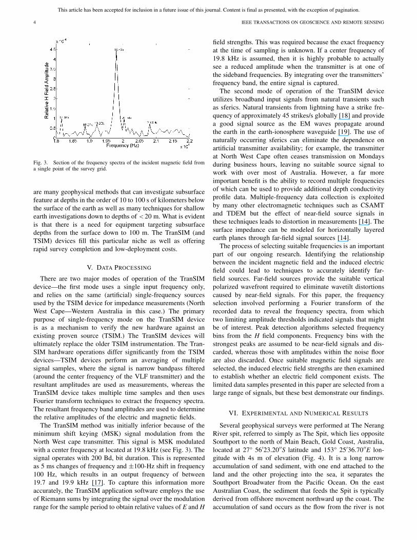
Several geophysical surveys were performed at The NerangRiver spit, referred to simply as The Spit, which lies oppositeSouthport to the north of Main Beach, Gold Coast, Australia,located at 27° 56′23.20′′S latitude and 153° 25′36.70′′E lon-gitude with 4s m of elevation (Fig. 4). It is a long narrowaccumulation of sand sediment, with one end attached to theland and the other projecting into the sea, it separates theSouthport Broadwater from the Pacific Ocean. On the eastAustralian Coast, the sediment that feeds the Spit is typicallyderived from offshore movement northward up the coast. Theaccumulation of sand occurs as the flow from the river is not

This article has been accepted for inclusion in a future issue of this journal. Content is final as presented, with the exception of pagination.

MOGENSEN et al.: SURFACE IMPEDANCE MAPPING 5

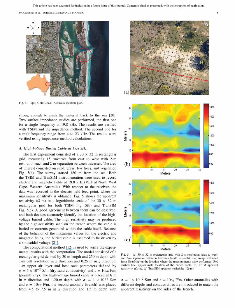
Fig. 4. Spit, Gold Coast, Australia location plan.

strong enough to push the material back to the sea [20].Two surface impedance studies are performed, the first onefor a single frequency at 19.8 kHz. The results are verifiedwith TSIM and the impedance method. The second one fora multifrequency range from 4 to 23 kHz. The results wereverified using impedance method calculations.

A. High-Voltage Buried Cable at 19.8 kHz

The first experiment consisted of a 30 × 32 m rectangulargrid, measuring 15 traverses from east to west with 2-mresolution each and 2-m separation between traverses. The areaof interest consisted on sand, grass, few trees, and vegetationFig. 5(a). The survey started 180 m from the sea. Boththe TSIM and TranSIM instrumentation were used to recordelectric and magnetic fields at 19.8 kHz (VLF at North WestCape, Western Australia). With respect to the receiver, thedata was recorded in the electric field feed point, where themaximum sensitivity is obtained. Fig. 5 shows the apparentresistivity (�-m) in a logarithmic scale of the 30 × 32 mrectangular grid for both TSIM Fig. 5(b) and TranSIMFig. 5(c). A good agreement between them can be observed,and both devices accurately identify the location of the high-voltage buried cable. The high resistivity may be producedby the high-resistivity sand on the trench where the cable isburied or currents generated within the cable itself. Becauseof the behavior of the maximum values for the electric andmagnetic fields, the buried cable is assumed to be driven bya sinusoidal voltage [21].

The computational method [12] is used to verify the experi-mental results with the computation. The model consisted of arectangular grid defined by 30 m length and 250 m depth with1-m cell resolution in x direction and 0.25 m in z direction,1-m upper air layer and host rock parameters defined byσ = 5 × 10−2 S/m (dry sand conductivity) and ε = 10ε0 F/m(permittivity). The high-voltage buried cable is placed at 6 min x direction and 1.20-m depth with σ = 1 × 10+6 S/mand ε = 10ε0 F/m, the second anomaly (trench) was placedfrom 4.5 to 7.5 m in x direction and 1.5 m depth with

Fig. 5. (a) 30 × 32 m rectangular grid with 2-m resolution (east to west)and 2-m separation between traverses (north to south), map image extractedfrom NearMap on the location where the measurements were performed. Reddashed line: approximate location of the buried cable. (b) TSIM apparentresistivity (�-m). (c) TranSIM apparent resistivity (�-m).

σ = 1 × 10−2 S/m and ε = 10ε0 F/m. Other anomalies withdifferent depths and conductivities are introduced to match theapparent resistivity on the sides of the trench.

This article has been accepted for inclusion in a future issue of this journal. Content is final as presented, with the exception of pagination.

6 IEEE TRANSACTIONS ON GEOSCIENCE AND REMOTE SENSING

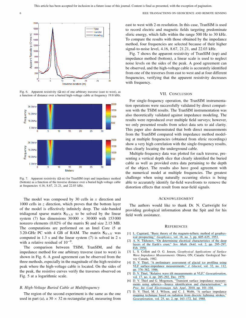
Fig. 6. Apparent resistivity (�-m) of one arbitrary traverse (east to west), asa function of distance over a buried high-voltage cable at frequency 19.8 kHz.

Fig. 7. Apparent resistivity (�-m) for TranSIM (top) and impedance method(bottom) as a function of the traverse distance over a buried high-voltage cableat frequencies 4.16, 8.67, 21.21, and 22.03 kHz.

The model was composed by 30 cells in x direction and1000 cells in z direction, which proves that the bottom layerof the model is effectively infinitely deep. The side-bandedtridiagonal sparse matrix SN×N to be solved by the linearsystem (7) has dimensions 30 000 × 30 000 with 153 000nonzero elements (0.02% of the matrix S) and size 2.15 MB.The computations are performed on an Intel Core i5 at3.20-GHz PC with 4 GB of RAM. The matrix SN×N wascomputed in 1.3 s and the linear system (7) is solved in 2 swith a relative residual of 10−9.

The comparison between TSIM, TranSIM, and theimpedance method for one arbitrary traverse (east to west) isshown in Fig. 6. A good agreement can be observed from thethree methods, especially in the magnitude of the high resistivepeak where the high-voltage cable is located. On the sides ofthe peak, the resistive curves verify the traverses observed onFig. 5 at a logarithmic scale.

B. High-Voltage Buried Cable at Multifrequency

The region of the second experiment is the same as the oneused in part (a), a 30 × 32 m rectangular grid, measuring from

east to west with 2-m resolution. In this case, TranSIM is usedto record electric and magnetic fields targeting predominatesferic energy, which falls within the range 500 Hz to 30 kHz.To compare the results with those obtained by the impedancemethod, four frequencies are selected because of their highersignal-to-noise level, 4.16, 8.67, 21.21, and 22.03 kHz.

Fig. 7 shows the apparent resistivity of TranSIM (top) andimpedance method (bottom), a linear scale is used to neglectnoise levels on the sides of the peak. A good agreement canbe observed, and the high-voltage cable is accurately identifiedfrom one of the traverses from east to west and at four differentfrequencies, verifying that the apparent resistivity decreaseswith frequency.

VII. CONCLUSION

For single-frequency operation, the TranSIM instrumenta-tion operations were successfully validated by direct compari-son with the TSIM results. The TranSIM instrumentation wasalso theoretically validated against impedance modeling. Theresults were reproduced over multiple field surveys; however,we only presented results from select data sets to aid clarity.This paper also demonstrated that both direct measurementsfrom the TranSIM compared with impedance method model-ing at multiple frequencies (obtained from sferic recordings)show a very high correlation with the single-frequency results,thus clearly locating the underground cable.

Multiple-frequency data was plotted for each traverse, pre-senting a vertical depth slice that clearly identified the buriedcable as well as provided extra data pertaining to the depthof the object. The results also have good agreement withthe numerical model at multiple frequencies. The greatestchallenge when using naturally occurring sferics is beingable to accurately identify far-field wavefronts to remove thedistortion effects that result from near-field signals.

ACKNOWLEDGMENT

The authors would like to thank Dr. N. Cartwright forproviding geological information about the Spit and for hisfield work assistance.

REFERENCES

[1] L. Cagniard, “Basic theory of the magneto-telluric method of geophys-ical prospecting,” Geophysics, vol. 18, no. 3, pp. 605–635, 1953.

[2] A. N. Tikhonov, “On determining electrical characteristics of the deeplayers of the Earth’s crust,” Sov. Math. Dokl, vol. 2, pp. 295–297,Feb. 1950.

[3] L. S. Collett and O. G. Jensen, Geophysical Applications of SurfaceWave Impedance Measurements. Ottawa, ON, Canada: Geological Sur-vey Canada, 1982.

[4] D. V. Thiel, “A preliminary assessment of glacial ice profiling usingVLF surface-impedance measurements,” J. Glaciol, vol. 32, no. 112,pp. 376–382, 1986.

[5] D. V. Thiel, “Relative wave tilt measurements at VLF,” Geoexploration,vol. 17, no. 4, pp. 285–292, Dec. 1979.

[6] D. V. Thiel and G. Mogensen, “Transient surface impedance measure-ments using spherics—Source identification and characterisation,” inProc. Int. Conf. Electromagn. Adv. Appl., 2010, pp. 101–104.

[7] D. V. Thiel, M. J. Wilson, and C. J. Webb, “A surface impedancemapping technique based on radiation from discrete lightning strokes,”Geoexploration, vol. 25, no. 2, pp. 163–172, Jul. 1988.

This article has been accepted for inclusion in a future issue of this journal. Content is final as presented, with the exception of pagination.

MOGENSEN et al.: SURFACE IMPEDANCE MAPPING 7

[8] S. A. Cummer, “Lightning and ionospheric remote sensing usingVLF/ELF radio atmospherics,” Ph.D. dissertation, Dept. Electr. Eng.,Stanford Univ., Palo Alto, CA, USA, 1997.

[9] R. Barr, D. L. Jones, and C. J. Rodger, “ELF and VLF radio waves,”J. Atmosph. Solar-Terrestrial Phys., vol. 62, nos. 17–18, pp. 1689–1718,2000.

[10] J. Henry, A. Buck, K. Henderson, and W. Smyth, “The application ofTSIM in defining sills in coal seams: A case study at Coppabella Mine,”in Proc. Austral. Soc. Explorat. Geophys., Feb. 2012, pp. 1–2.

[11] D. V. Thiel and R. Mittra, “A self-consistent method for electromagneticsurface impedance modelling,” Radio Sci., vol. 36, no. 1, pp. 31–43,2001.

[12] H. G. Espinosa and D. V. Thiel, “Efficient forward modelling ofelectromagnetic surface impedance for coal seam assessment,” in Proc.Austral. Soc. Explorat. Geophys., Feb. 2012, pp. 1–4.

[13] Y. Saad, Iterative Methods for Sparse Linear Systems, 2nd ed. Philadel-phia, PA, USA: SIAM, 2003.

[14] J. R. Wait, Electromagnetic Waves in Stratified Media. Oxford, U.K.:Pergamon, 1962.

[15] G. Porstendorfer, Principles of Magneto-Telluric Prospecting. Berlin,Germany: Borntraeger, 1975.

[16] M. Unsworth, W. Wenbo, A. G. Jones, S. Li, P. Bedrosian, J. Booker,J. Sheng, D. Ming, and T. Handong, “Crustal and upper mantle structureof northern Tibet imaged with magnetotelluric data,” J. Geophys. Res.,vol. 109, no. B2, p. B02403, Feb. 2004.

[17] M. B. Cohen, U. S. Inan, and E. W. Paschal, “Sensitive broadbandELF/VLF radio reception with the AWESOME instrument,” IEEE Trans.Geosci. Remote Sens., vol. 48, no. 1, pp. 3–17, Jan. 2010.

[18] H. J. Christian, “Global frequency and distribution of lightning asobserved from space by the optical transient detector,” J. Geophys. Res.,vol. 108, no. D1, pp. ACL 4-1–ACL 4-16, 2003.

[19] A. D. Watt and R. D. Croghan, “Comparison of observed VLF atten-uation rates and excitation factors with theory (very low frequencypropagation modes observed, comparing calculated attenuation rates andexcitation factors with theory),” J. Res., Radio Sci., vol. 68D, pp. 1–9,Jan. 1964.

[20] R. Whitlow, “A Geomorphological outline of the spit and the south-ern Broadwater, Gold Coast, Queensland: Their environmental history& modifications,” TriMAP Pty Ltd, Nerang, Australia, Tech. Rep.,Jul. 2005.

[21] M. Sitepu and D. V. Thiel, “The surface impedance anomaly resultingfrom a subsurface, infinitely long conductive wire,” IEEE Trans. Geosci.Remote Sens., vol. 29, no. 2, pp. 314–320, Mar. 1991.

Gavin T. Mogensen received a degree in Micro-electronic Engineering from Griffith University,Brisbane, Australia in 1996.

He has worked as a professional engineerin various fields from medical research, gam-ing industry, and more recently within the min-ing industry. Currently he is a PhD candidatewith Griffith University’s “Center for WirelessMonitoring and Applications” researching the appli-cation of transient signals for use in geophysicalprospecting.

Hugo G. Espinosa was born in Mexico City in1976. He received the B.Sc. degree in Electron-ics and Telecommunications Engineering from theMonterrey Institute of Technology, Mexico, in 1998,the MSc degree from the University of Sao Paulo,Brazil, in 2002, and the PhD degree (summa cumlaude) from the Technical University of Catalonia,Spain, in 2008, both in Electrical Engineering.

In 2006 he joined the Federal Polytechnic Schoolof Lausanne, Switzerland, for a four-month researchstay. From 2009 to 2010, he has been a post-doc

fellow with the Physical Electronics Department of the School of ElectricalEngineering at Tel Aviv University, Israel. Since 2011, he is with the Centrefor Wireless Monitoring and Applications of the School of Engineering atGriffith University, Australia, where he is currently a Research Fellow.

His main research interests include fast methods for numerical computationof electromagnetic scattering and radiation.

David V. Thiel (SM’88) received a B.Sc. degreefrom the University of Adelaide, Adelaide, Australia,in 1970, and then completed his M.Sc. and PhDdegrees from James Cook University, Townsville,Australia, in 1974 and 1980, respectively. He is cur-rently Professor in the Griffith School of Engineeringand Director of the Centre for Wireless Monitoringand Applications at Griffith University.

He is a Fellow of the Engineers Australia. Heserves as Chair of the Wave Propagation StandardsCommittee of the IEEE Antennas and Propagation

Society and is a member of the Antennas Standards Committee.Prof. Thiel worked with the team that developed the world’s first odor

sensing robot. He led the development of TSIM, a surface impedance meterused in Central Queensland coalfields for pre-mining coal seam assessment.He has several patents and has published over 100 journal papers and 150conference papers and presentations. His current research interests includesmart antennas, numerical modelling in electromagnetics, electromagneticgeophysics, sports technologies, wireless sensor networks, and novel circuitmanufacturing techniques.