Surface detection of alkaline ultramafic rocks in semi-arid and ...

Open Research OnlineThe Open University’s repository of research publicationsand other research outputs

Surface detection of alkaline ultramafic rocks insemi-arid and arid terrains using spectral geologicaltechniquesThesisHow to cite:

Hussey, Michael Charles (1999). Surface detection of alkaline ultramafic rocks in semi-arid and arid terrainsusing spectral geological techniques. PhD thesis The Open University.

For guidance on citations see FAQs.

c© 1998 The Author

https://creativecommons.org/licenses/by-nc-nd/4.0/

Version: Version of Record

Link(s) to article on publisher’s website:http://dx.doi.org/doi:10.21954/ou.ro.0000d3a2

Copyright and Moral Rights for the articles on this site are retained by the individual authors and/or other copyrightowners. For more information on Open Research Online’s data policy on reuse of materials please consult the policiespage.

oro.open.ac.uk

SURFACE DETECTION OF ALKALINE ULTRAMAFIC ROCKS IN SEMI-ARID AND

ARID TERRAINS USING SPECTRAL GEOLOGICAL TECHNIQUES

A thesis submitted for the degree of Doctor of Philosophy

By

Michael Charles Hussey B.Sc. (Hons) Southampton

Department of Earth Sciences The Open University

June, 1998

VOLUME2of2

'. m (04 742-. ,~ C. \

TABLE OF CONTENTS

VOLUMEl ABSTRACT DEDICATION AKNOWLEDGEMENTS TABLE OF CONTENTS LIST OF FIGURES LIST OF TABLES

1 INTRODUCTION 1.1 ST ATEMENT OF OBJECTIVES 1.2 SPECTRAL GEOLOGICAL DEVELOPMENT 1.3 ALKLINE ULTRAMAFIC ROCKS 1.4 REMOTE SENSING APPLIED TO ULTRAMAFIC ROCKS. 1.5 GEOGRAPHIC RANGE OF INVESTIGATIONS 1.6 STRUCTURE OF THESIS 1.7 CONTRmUTIONS

2 PREVIOUS INVESTIGATIONS. 2.1 INTRODUCTION 2.2 REVIEWS

Field Studies Landsat MSS Landsat TM Landsat TM and JERS-l OPS GEOSCAN MkII AIS. GER IS. AVIRIS

2.2 CONCLUSIONS.

3 SPECTRAL GEOLOGICAL CONCEPTS, INSTRUMENTS, AND TECHNIQUES INVESTIGATED.

3.1 INTRODUCTION 3.2 SPECTRAL REGIONS INVESTIGATED 3.3 FIELD AND THE LABORATORY SPECTROMETERS

The GER MkIV IRIS Spectrometer The PIMA Spectrometer

3.4 PROCESSING OF SPECTROMETER DATA Spectral Processing Techniques

3.5 SCANNER IMAGING SYSTEMS Airborne Scanners Design Airborne Scanner Classification

3.6 PROCESSING OF SCANNER DATA Conversion of Raw Data to Radiance and Reflectance Image Processing Software Conventional Image Processing Spectral Methods

3.7 MODELLING OF SCANNER SPECTRA

IV

1-1 1-1 1-7 1-9 / 1-10 1-12 1-13

2.1 2-1 2-1 2-2 2-3 2-3 2-8 2-10 2-10 2-11 2-12 2-13

3-1 3-1 3-2 3-3 3-3 3-4 3.4 3.9 3-9

3-10 3-11 3-12 3-16 3-17 3-21 3-24

4 THE MINERALOGY AND WEATHERING OF ALKALINE AND OTHER ULTRAMAFIC ROCKS; IMPLICATIONS FOR SURFACE SPECTRAL EXPRESSION

4.1 INTRODUCTION 4-1 4.2 CLASSIFICATION AND MINERALOGY OF ULTRAMAFIC ROCKS 4-1 4.3 WEATHERING OF ULTRAMAFIC ROCKS 4-4

Weathering in Arid Regions 4-4 Australian Weathering Conditions 4-7 Weathering in Areas Studied 4-11

4.4 WEATHERING PRODUCTS OF NON-ULTRAMAFIC ROCKS 4-12 4.5 CONCLUSIONS 4-13

5 DETERMINATION OF THE SPECTRA OF ALKALINE, OTHER ULTRAMAFIC AND BACKGROUND ROCKS

5.1 INTRODUCTION 5-1 5.2 LABORATORYSPECTRALSTUDlliS 5-1 5.3 SURFACEFlliLDSTUDlliS 5-3

In Situ versus Laboratory Measurements 5-4 5.4 ULTRAMAFIC ROCK SPECTRA 5-5

Fresh Rock Spectra 5-6 Weathered Rock Spectra 5-9

5.5 SPECTRA OF SOILS DERIVED FROM ULTRAMAFIC ROCKS 5-11 5.6 BACKGROUND ROCKS (AND MATERIALS) INCLUDING THOSE

SPECTRALLY SIMILAR TO ULTRAMAFIC ROCKS 5-12 5.7 CONCLUSIONS 5-16

v

6 MINERAL MIXING AND THE SPECTRAL RESPONSE OF ALKALINE ULTRAMAFIC ROCKS AND DERIVED SOILS INTRODUCTION 6-1

6.2 KAOLINITE - SAPONITE 6-3 Physical Mixtures 6-3 Virtual Mixtures 6-4 Virtual Library Mixtures 6-5 Comments 6-7

6.3 SAPONITE - ILLITE 6-7 Physical Mixtures 6-7 Virtual Mixtures 6-8 Virtual Library Mixtures 6-9 Comment 6-11

6.4 SAPONITE - DOLOMITE 6-11 Physical Mixtures 6-11 Library Virtual Mixtures 6-14 Virtual Library Mixtures 6-15 Comments 6-15

6.5 SAPONITE AND LIMESTONE 6-16 Physical Mixture 6-16 Virtual Mixtures 6-17

6.6 SAPONITE AND DRY VEGETATION 6-18 Physical Mixtures 6-18 Virtual Mixtures 6-19 Comment 6-20

6.7 VIRTUAL MIXTURES TO SIMULATE ULTRAMAFIC ROCKS SURFACES AND SOIL SPECTRAL EXPRESSION 6-21 Saponite-Quartz Sand Mixtures 6-21 Saponite-Kaolinite-Quartz Mixtures (soil derived from ultramafic rocks) 6-22

6.8 OTHER MINERAL MIXTURES 6-23 6.9 CONCLUSIONS 6-24

7 SPECTRAL CHARACTERISTICS OF REMOTE SENSING SYSTEMS COMPARED TO THE ULTRAMAFIC MODEL AND SIGNAL-TO-NOISE

7.1 INTRODUCTION 7-1 7.2 SIMULATED SYSTEM SPECTRA 7-2

Multispectral Scanners 7-3 Imaging Spectrometers 7-4 Hyperspectral Scanners 7-5

7.3 SIGNAL-TO-NOISE RATIO 7-7 HyMap Spectra 7-10 GEOSCAN MkII Spectra 7-12 Noise Reduction Filtering 7-13

7.4 CONCLUSIONS 7-15

VI

8 EVALUATION OF CONVENTIONAL IMAGE PROCESSING TECHNIQUES USING SIMULATED SCANNER DATA

8.1 INTRODUCTION 8-1 Spectral Feature Enhancement 8-2

8.2 SIMULATED IMAGERY 8-4 Field Examples 8-5

8.3 ATMOSPHERIC CORRECTION 8-5 Methods 8-5 Test Results 8-7

8.4 GEOSCAN MkII OFFSETS 8-9 8.5 LANDSAT TIM PROCESSING 8-11

Band Ratios 8-11 Clay Prediction Techniques 8-15 Quick Residual Processing 8-16 Crosta Principal Component Transform (Crosta Technique) 8-19 Mixed Composite Images 8-20 Comments 8-21

8.6 GEOSCAN MkII PROCESSING 8-22 Quick Residual Processing 8-22 Crosta Principal Component Transform 8-23 Effects of Noise on Crosta Technique 8-24

8.7 GER 32 BAND (SWIR2) PROCESSING 8-24 Quick Residual Processing 8-24 Crosta Principal Component Transform 8-25

8.8 MERIDTH DATA 8-26 GEOSCAN MkII Simulated Image 8-28 GER 32 Band Simulated Image 8-29

8.9 CONCLUSIONS 8-33

VOLUME 2

9 TEST SITE STUDY PINE CREEK, TEROWIE DISTRICT, SOUTH AUSTRALIA

9.1 INTRODUCTION 9-1 9.2 GEOLOGICAL SETTING 9-2

Kimberlites 9-3 9.3 FIELD STUDIES 9-4

Spectral Response of the Kimberlite 9-4 Spectral Response of Soil derived from Kimberlite 9-5 Surface Spectral Mapping 9-8 Vegetation Cover 9-10

9.4 GROUND BASED SPECTRAL ANALYSIS OF KIMBERLITE AND BACKGROUND SOILS FROM PINE CREEK USING THE GEOSCAN MK II SCANNER 9-14 Procedures 9-15 Analysis 9-16 Comments and Conclusions 9-20

9.5 IMAGE PROCESSING OF HyMap SCANNER DATA 9-20 Conventional Processing 9-20 Spectral Processing 9-28 Comments 9-32

9.6 CONCLUSIONS FROM PINE CREEK SPECTRAL STUDIES 9-33

VII

10 TEST SITE STUDY· JUBILEE, KURNALPI AREA, WESTERN AUSTRALIA

10.1 INTRODUCTION 10-1 10.2 FIELD STUDIES 10-3 10.3 IMAGE PROCESSING - DATA SETS 10-4 lOA GEOSCAN MkII DATA 10-5

Conventional Image Processing 10-6 Spectral Processing 10-10

10.5 GER IS DATA 10-12 Conventional Processing 10-12 Spectral Processing 10-15

10.6 HyMap DATA 10-17 Conventional Processing 10-17 Spectral Processing 10-23

10.7 CONCLUSIONS 10-25

11 TEST SITE STUDY· 81·MILE VENT, ELLENDALE AREA, WESTERN AUSTRALIA

11.1 INTRODUCTION 11-1 11.2 FIELD STUDIES 11-2 11.3 IMAGE PROCESSING - DATA SETS 11-4 11.4 GEOSCAN MkII DATA 11-5

Conventional Image Processing 11-5 Spectral Processing 11-8

11.5 HyMap DATA 11-9 Conventional Processing 11-9 Spectral Processing 11-15

11.6 CONCLUSIONS 11-17

12 CONCLUSIONS AND RECOMMENDATIONS FOR FURTHER STUDIES 12.1 CONCLUSIONS 12-1

Diagnostic Spectral Signature of Alkaline ultramafic rocks 12-2 Spectral signature of the weathering products of ultramafic rocks 12-2 Non Ultramafic Rock Signatures 12-3 Spectra of Mineral Mixtures 12-3 Line Scanning Systems Specifications 12-4 Data Processing Techniques 12-7 Simulated Data 12-8 Test Site Studies 12-9

12.2 RECOMMENDATIONS FOR FURTHER INVESTIGATIONS 12-11

VIII

GLOSSARY

LIST OF REFERENCES

APPENDIX 1: SPECIFICATIONS OF FIELD SPECTROMETERS

APPENDIX 2: BAND CENTRES USED TO SAMPLE SPECTRA

APPENDIX 3: MODELLING SOFTWARE

APEENDIX 4: SPECTRAL CALIBRATION OF GEOSCAN MkII DATA

IX

2 pages

8 pages

1 page

7 pages

14 pages

19 pages

LIST OF FIGURES CHAPTER!

Figure 1.1: Mineral map derived from A VIRIS data obtained over Cuprite, Nevada, in 1995. Figure 1.2: A VIRIS sites from the JPL web page Figure 1.3: Phytohydroxic index map of Australia. Figure 1.4: Photographs showing landscape at Pine Creek, Jubilee and Ellendale sites.

CHAPTER 3

Figure 3.1: VNIR Spectra of Iron Oxide bearing minerals. Figure 3.2: Examples of SWIR spectra. Figure 3.3: Serpentine spectra. Figure 3.4: Effects of linear scaling, spectra Figure 3.5: Stacked profile spectra. Figure 3.6: Hull quotient and Hull difference spectra. Figure 3.7: Spectra of kaolinite (grey) and serpentine (black). Figure 3.8: Schematic of a modern HyMap optical mechanical scanner. Figure 3.9 Image log residual transformed spectrum. Figure 3.10: X Profile over a Mg-OH anomaly obtained. Figure 3.11: Index images produced by thresholding and un-mixed image. Figure 3.12: Plot showing band passes for GEOSCAN MkII scanner. Figure 3.13: Comparison of two methods ofre-sampling a talc spectrum.

CHAPTER 4

Figure 4.1: Kimberlite model after Hawthorn (1975). Figure 4.2: VNIR spectra of some typical ultramafic rock minerals. Figure 4.3: SWIR2 spectra of minerals. Figure 4.4: Stacked spectra (A) and vertical soil profiles (B) from a kimberlite. Figure 4.5: Sketch (after Butt, 1981) showing variation in lateritic profile. Figure 4.6:HyMap end-member un-mixed image. Figure 4.7:Model spectra proposed for weathered ultramafic rocks.

CHAPTERS

Figure 5.1: GER MkIV spectrometer set up in a laboratory. Figure 5.2: PIMA set up in a laboratory. Figure 5.3: GER IRIS MkIV in the field during 1986. Figure 5.4: Spectra obtained from same sample material in the laboratory and field. Figure 5.5: Example spectra taken from the surface and sub-surface. Figure 5.6: VNIR to SWIR2 reflectance spectra of fresh surfaces of ultramafic rocks. Figure 5.7: VNIR to SWIR2 hull quotient spectra of ultramafic rocks. Figure 5.8: Stacked hull quotient spectra of kimberlite facies changes for the SWIR2. Figure 5.9: SWIR2 spectra of hydroxyl bearing minerals typical of ultramafic rocks. Figure 5.10: VNIR to SWIR reflectance spectra of weathered surfaces of ultramafic rocks. Figure 5.11 Stacked SWIR2 hull quotient spectra of soils. Figure 5.12 Stacked SWIR2 hull quotient spectra of minerals. Figure 5. 13: Stacked SWIR2 hull quotient spectra of igneous rocks. Figure 5.14: Stacked SWIR2 hull quotient spectra of sedimentary rocks. Figure 5.15 Stacked SWIR hull quotient spectra of metamorphic rocks.

X

1-4 1-7 1-11 1-12

3-2 3-2 3-5 3-6 3-6 3-7 3-8 3-10 3-16 3-20 3-20 3-25 3-26

4-2 4-3 4-4 4-6 4-8 4-10 4-11

5-2 5-2 5-3 5-4 5-5 5-6 5-7 5-7 5-9 5-10 5-12 5-14 5-15 5-15 5-16

CHAPTER 6

Figure 6.1: Stacked hull quotient spectra of physical mixtures of saponite and kaolinite. Figure 6.2: Plot of Mg Score ratio values calculated from the saponite-kaolinite. Figure 6.3: Stacked hull quotient spectra of virtual mixtures of saponite and kaolinite. Figure 6.4: Plot of Mg Score ratio values calculated from the saponite-kaolinite. Figure 6.5: Stacked hull quotient spectra of virtual library mixtures of saponite and kaolinite Figure 6.6: Plot of Mg Score ratio values calculated from saponite-kaolinite spectra. Figure 6.7: Stacked hull quotient spectra of physical mixtures of saponite and illite. Figure 6.8: Plot ofMg Score ratio values calculated from saponite-illite spectra. Figure 6.9: Stacked hull quotient spectra of virtual mixtures of saponite and illite. Figure 6.10: Plot ofMg Score ratio values calculated from the virtual saponite-illite spectra. Figure 6.11: Stacked hull quotient spectra of virtual library mixtures of saponite and illite. Figure 6.12: Plot ofMg Score ratio values calculated from saponite-illite spectra. Figure 6.13: Stacked Hull Quotient spectra of physical mixture saponite and dolomite Figure 6.14: Plot ofthe saponite-dolomite physical mixture spectra. Figure 6.15: Plot for the saponite-dolornite physical mixture spectral gradient. Figure 6.16: Stacked hull quotient profile of spectra for virtual mixtures. Figure 6.17: Plot of saponite-dolomite virtual mixed spectra. Figure 6.18: Plot oft the saponite-dolomite virtual mixture spectral gradient. Figure 6.19: Stacked hull quotient of saponite and dolomite spectra. Figure 6.20: Plot of saponite-dolomite library virtual mixture spectra. Figure 6.21: Stacked hull quotient spectra of saponite and limestone. Figure 6.22: Plot of saponite-Iimestone physical mixture Spectra. Figure 6.23: Stacked hull quotient spectra for the virtual saponite and limestone. Figure 6.24: Stacked hull quotient spectra for physical mixtures of saponite and dry vegetation. Figure 6.25: Plot of saponite-dry vegetation physical mixtures ratio values. Figure 6.26: Stacked hull quotient spectra of virtual mixtures of saponite and dry vegetation. Figure 6.27: Plot of saponite-dry vegetation virtual mixtures ratio values. Figure 6.28: Spectra of pure quartz saponite and a virtual mixture. Figure 6.29: Hull quotient transformed spectra of saponite, kaolinite. Figure 6.30: Hull quotient transformed virtual mixed spectrum of saponite, kaolinite and quartz. Figure 6.31: Hull quotient transformed virtual 50 percent: 50 percent mixed spectrum.

CHAPTER 7

Figure 7.1: Virtual hull quotient spectra that model the ultramafic outcrops. Figure 7.2: JERS OPS sampled SWIR2 hull quotient spectra .. Figure 7.3: ASTER sampled hull quotient SWIR2 spectra, Figure 7.4: GEOSCAN MkII sampled hull quotient SWIR2 spectra. Figure 7.5: GER IS hull quotient sampled spectra SWIRl and SWIR2 regions. Figure 7.6: GER DIAS hull quotient sampled spectra SWIRl and SWIR2 regions. Figure 7.7: DAEDALUS MIVIS hull quotient sampled spectra SWIRl and SWIR2 regions. Figure 7.8: ARIES hull quotient sampled spectra SWIRl and SWIR2 regions. Figure 7.9: HyMap hull quotient sampled spectra SWIR2 region. Figure 7.10: PIMA reflectance spectrum sampled to HyMap bands Figure 7.11: PIMA hull quotient stacked spectra sampled to HyMap bands. Figure 7.12: PIMA reflectance spectrum sampled to GEOSCAN MKII bands. Figure 7.13: PIMA hull quotient stacked spectra sampled to GEOSCAN MKII bands Figure 7.14: Un-filtered PIMA reflectance saponite-kaolinite spectra .. Figure 7.15: FFf filtered PIMA reflectance saponite-kaolinite spectra.

XI

6-4 6-4 6-5 6-5 6-6 6-6 6-8 6-8 6-9 6-9 6-10 6-10 6-11 6-12 6-12 6-13 6-13 6-14 6-15 6-15 6-16 6-17 6-17 6-18 6-19 6-19 6-20 6-22 6-23 6- 23 6-24

7-3 7-4 7-4 7-5 7-5 7-6 7-6 7-6 7-7 7-10 7-11 7-12 7-13 7-15 7-15

CHAPfER8

Figure 8.1: Geology and Regolith from Landsat TM imagery. Figure 8.2: RIM - scattergram plot of pixels DNs of two sites from TM imagery. Figure 8.3: Arithmetic ratio images. Figure 8.4: Arithmetic ratio images. Figure 8.5: Arithmetic ratio colour composite of TM band ratios 5/6(7),311 and 4/3. Figure 8.6 Anomaly Residual Prediction TM Band 6 image. Figure 8.7 TM directed principal components Figure 8.8: Quick residual image (negative) from bands 1-6. Figure 8.9: Quick Residual Colour Composite simulated TM Bands 6,1,3 Figure 8.10 Hydroxyl Crosta Principal Component 3. Figure 8.11: Iron mineral Crosta principal component 1. Figure 8.12: Mixed colour composite of band prediction. Figure 8.13: GEOSCAN MkII SWIR2 quick residual colour composite. Figure 8.14: GEOSCAN MkII Crosta technique index image of principal component 3. Figure 8.15: GER 32 Band quick residual colour composite Mg-OH minerals. Figure 8.16 GER 32 Band Crosta PC 3 index image Figure 8.17: Meredith melnoite grid MgScore ratio showing the Melnoite contact. Figure 8.18: Meredith melnoite grid PIMA Figure 8.19: Meredith melnoite grid GEOSCAN MkII simulated CC image. Figure 8.20: Meredith melnoite grid GEOSCAN MkII simulated Crosta image Figure 8.21: Meredith melnoite grid GER 32 Band simulated image. Figure 8.22: Meredith melnoite grid GER 32 Band simulated image. Crosta. Figure 8.23: Meredith melnoite grid GER 32 Band simulated image showing effects of noise Figure 8.24: Plot of noise versus standard deviation

CHAPfER9

Figure 9: 1: Location map of the Pine Creek area showing HyMap flight line. Figure 9.2: Geology map of Pine Creek area (after Cowley and Priess, 1997) Figure 9.3: Average spectra (hull quotient transformed) of Pine Creek OJ kimberlite. Figure 9.4: Pine Creek 01 grid Mg Ratio Score contour plot. Figure 9.5: Stacked profile of spectra (hull difference transformed) augur hole. Figure 9.6: Pine Creek 01 hull quotient transformed Mg-OH and AI-OH soil spectra Figure 9.7:Pine Creek 01 Mg Score ratio value plotted as a profile. Figure 9.8:Pine Creek region calc-arenite and background soil hull quotient spectra. Figure 9.9: PC8 and PC9 HyMap Mg Score ratio contours maps. Figure 9.10: Photo interpretation of vegetation cover. Figure 9.11: Pine Creek vegetation study. Figure 9.12: Pine Creek OJ soil and black lichen. Figure 9.13: Sketch showing location of GEOSCAN MkII samples. Figure 9.14: GEOSCAN MkII Scanner set up to measure spectra from soil samples. Figure 9.15: PIMA spectra of the samples measured with GEOSCAN MkII scanner. Figure 9.16: Hull quotient PIMA spectra of samples measured with GEOSCAN Mkii. Figure 9.17: PIMA spectra sampled to GEOSCAN MkiI scanner bands. Figure 9.18: Un-calibrated spectra obtained from GEOSCAN MkII scanner. Figure 9.19: Calibrated spectra obtained from GEOSCAN MkII. Figure 9:20: Calibrated and log residual transformed spectra from GEOSCAN MkII Figure 9.21: HyMap image showing location of Pine Creek 01 kimberlite. Figure 9.22: HyMap colour composite image of the negative of raw image bands. Figure 9.23: HyMap colour composite of log residual transformed image. Figure 9.24: Spectrum extracted from log residual transformed data. Figure 9.25: Spectrum extracted from log residual transformed data. Figure 9.26: Spectrum extracted from log residual transformed data. Figure 9.27: HyMap Mg Score ratio image of log residual transformed image. Figure 9.28: HyMap Crosta principal component transform index image. Figure 9.29: HyMap anomaly prediction index image of 2306nm band predicted. Figure 9.30: HyMap Mg-OH mineral end-member spectrum.

XII

8-3 8-6 8-12 8-13 8-14 8-15 8-16 8-17 8-18 8-19 8-20 8-21 8-22 8-23 8-25 8-26 8-27 8-27 8-28 8-29 8-30 8-31 8-32 8-33

9-1 9-3 9-5 9-6 9-7 9-8 9-9 9-9 9-9 9-11 9-12 9-13 9-15 9-15 9-17 9-17 9-18 9-18 9-19 9-19 9-22 9-23 9-24 9-24 9-25 9-25 9-26 9-27 9-28 9-28

Figure 9.31: HyMap un-mixed index image for Mg-OH end-membcr spectra. Figure 9.32: Results of end-member un-mixing. Figure 9:33: HyMap dolomite end-member spectrum. Figure 9:33: HyMap dolomite end-member spectrum. Figure 9:34: HyMap AI-OH end-member spectrum. Figure 9.35: HyMap Mg-OHlAI-OH mineral end-members un-mixed image.

CHAPTER 10

Figure 10.1: Location Map Jubilee Area. Figure 10.2: Geological sketch map of Jubilee ultramafic outcrop Figure 10.3: Field spectra from Jubilee grid spectral hull quotient transformed. Figure 10.4: Jubilee GEOSCAN MklI negative colour composite. Figure 10.5: Jubilee GEOSCAN MklI negative colour composite Figure 10.6: GEOSCAN MidI average Mg-OH spectrum derived from log residual. Figure 10.7 is a spectrum obtained from an area of outcrop of clastic sediments. Figure 10.8: Jubilee GEOSCAN MidI Mg Score index image. Figure 10.9: Jubilee aEOSCAN MkII Crosta technique colour composite image Figure 10.10: Jubilee aEOSCAN MkII end-member Mg-OH spectrum. Figure 10.11: Jubilee GEOSCAN MkII Mg-OH end-member un-mixed index image. Figure 10.12: Jubilee GER IS negative colour composite of log residual transformed. Figure 10.13: Jubilee GER IS average Mg-OH spectrum Figure 10.14: Jubilee GER IS average AI-OH spectrum. Figure 10.15: Jubilee GER IS Mg Score ratio image. Figure 10.16: Jubilee GER IS Crosta index image. Figure 10.17: Jubilee GER IS end-member spectrum typical of Mg-OH minerals. Figure 10.18: Jubilee GER IS end-member spectrum typical of AI-OH minerals Figure 10.19: Jubilee GER IS end-member un-mixed colour composite image. Figure 10.20: Jubilee HyMap negative colour composite of raw data. Figure 10.21: Jubilee HyMap negative colour composite of log residual Figure 10.22 Jubilee HyMap log residual spectrum. Figure 10.23: Jubilee HyMap log residual spectrum Figure 10.24: Jubilee HyMap log residual spectrum. Figure 10.25: Jubilee HyMap Mg Score index image. Figure 10.26: Jubilee HyMap Crosta transform image Figure 10.27: Jubilee HyMap Crosta transform colour composite Image. Figure 1O.2S: Jubilee HyMap end-member spectra from log residual data. Figure 10.29: Jubilee HyMap un-mixed index image. Figure 10.30: Jubilee HyMap end-member spectra from log residual data.

CHAPTER 11

Figure 11.1: 81-Mile Vent location map and flight line flown with scanners. Figure 11.2: SI-Mile Vent lamproite mesa, aerial view from northwest. Figure 11.3: 81-Mile Vent geology map. Figure 11.4: 8 I-Mile Vent spectra obtained from grid samples Figure 11.5: 8 I-Mile Vent aEOSCAN MkII raw data negative colour composite. Figure 11.6: 8 I-Mile Vent GEOSCAN MkII log residual transformed colour composite. Figure 11.7: 8 I-Mile Vent aEOSCAN MidI Mg Score index image. Figure 11.8: 8 I-Mile Vent GEOSCAN MkII Crosta principal component image. Figure 11.9: 81-Mile Vent GEOSCAN MkiI log residual transform spectrum. Figure 11.10: 81-Mile Vent GEOSCAN MkII log residual transform end-member spectrum Figure 11.11: 81-Mile Vent GEOSCAN MkII un-mixed log residual transform image Figure 11.12: 81-Mile Vent HyMap raw data negative colour composite image. Figure 11.13: 81-Mile Vent HyMap log residual transformed colour composite Figure 11.l4: 81-Mile Vent lamproite HyMap log residual transform spectra. Figure 11.15: 81-Mile Vent lamproite HyMap log residual transform spectrum Figure 11.16: 81-Mile Vent lamproite HyMap log residual transform spectrum

XIII

9-29 9-30 9-30 9-30 9-31 9-31

10-1 10-3 10-4 10-6 10-7 10-7 IO-S 10-9 10-10 10-11 10-11 10-13 10-13 10-13 10-14 10-15 10-15 10-16 10-16 10-18 10-18 ]0-]9 10-19 10-20 10-21 10-22 10-23 10-24 10-24 10-25

ll-I 11-2 11-3 11-4 11-5 11-6 11-6 11-7 11-8 11-9 11-9 11-10 11-10 Il-ll 11-12 11-12

Figure 11.17: Hull Quotient transform of Log Residual spectra .. Figure 11.18: 81-Mile Vent HyMap log residual transformed Mg Score image. Figure 11.19: 81-Mile Vent HyMap log residual transformed Crosta image. Figure 11.20: 81-Mile Vent HyMap anomaly band prediction image. Figure 11.21: Spectrum from area in south east of Anomaly prediction image. Figure 11:22: 81 Mile Vent lamproite and C03 end-member spectra. Figure 11.23: 81-Mile Vent HyMap end-member un-mixed index image.

XIV

11-13 11-13 11-14 11-15 11-15 11-16 11-16

LIST OF TABLES

CHAPTERl

Table 1.1: Mineral deposits associated with ultramafic rocks 1-8 Table 1.2: Magnesium percentage content of common rocks compared to ultramafic rocks 1-8 Table 1.3: Magnesium percentage content of ultramafic rocks 1-9

CHAPTER 2

Table 2.1: Keywords and results of GEOBASEIGEOREF database search 2-1

CHAPTER 4

Table 4.1: Weathering products of minerals characteristic of ultramafic rocks in arid soils 4-5 Table 4.2: Weathering minerals produced from ultramafic rocks under different weathering 4-7

CHAPTERS

Table 5.1: Percentage depth of the SWIR2 absorption features 5-6 Table 5.2: Percentage depth of the SWIR2 absorption features 5-10 Table 5.3: Mg-OH bearing minerals that can occur in non-ultramafic rocks 5-13 Table 5.4: Minerals. rocks and other materials that have absorption features near 2300nm 5-14 Table 5.5: Distribution and percentage depth of diagnostic absorption features for minerals 5-17

CHAPTER 7

Table 7.1: System specifications of past and current spectral scanners Table 7.2: signal-to-noise ratio levels converted to noise percentages

CHAPTERS

7-2 7-8

Table 8.1: Scanner band wavelengths used for simulated images 8-4 Table 8.2: Results of testing various atmospheric correction techniques on simulated TM imagery 8-8 Table 8.3: Spreadsheet DN values for kaolinite for simulated GEOSCAN MkII offsets introduced 8-9 Table 8.4: Results of simulated kaolinite GEOSCAN MkII data with RM and Switzer techniques 8-10 Table 8.5: Results of calculating the ATl offsets using the simulated data 8-10

CHAPTER 9

Table 9.1: Pine Creek 01 augur hole spectral analysis Table 9.2: HyMap SWIR2 band centres in nm

CHAPTERlO

Table 10.1: GEOSCAN MkiI SWIR2 band centres TablelO.2: GER IS SWIR2 wavelengths

xv

9-7 9-21

10-5 10-12

CHAPTER 9

9 TEST SITE STUDY PINE CREEK, TEROWIE DISTRICT, SOUTH AUSTRALIA

9.1 INTRODUCTION

This test site was chosen as an example of an alkaline ultramafic rock, in this case

kimberlite, which is not exposed and has been eroded, weathered and covered by residual

soil.

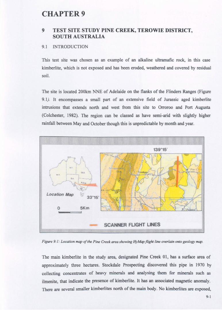
The site is located 200km NNE of Adelaide on the flanks of the Flinders Ranges (Figure

9.1). It encompasses a small part of an extensive field of Jurassic aged kimberlite

intrusions that extends north and west from this site to Orroroo and Port Augusta

(Colchester, 1982). The region can be classed as have semi-arid with slightly higher

rainfall between May and October though this is unpredictable by month and year.

(

Location Map

o SKm

SCANNER FLIGHT LINES

Figure 9: 1: Location map of the Pine Creek area showing HyMap flight line overlain onto geology map.

The main kimberlite in the study area, designated Pine Creek 01, has a surface area of

approximately three hectares. Stockdale Prospecting discovered this pipe in 1970 by

collecting concentrates of heavy minerals and analysing them for minerals such as

ilmenite, that indicate the presence of kimberlite. It has an associated magnetic anomaly.

There are several smaller kimberlites north of the main body. No kimberlites are exposed,

9-1

though surface disturbance, from diamond prospecting in the 1970s, has left patches of

kimberlitic clay on the surface at the Pine Creek 01 kimberlite.

The vegetation cover in the area is undisturbed and consists of a, variety of dry land plant

communities comprising open shrub and woodland. Lewis (1996) determined that the

various plant communities result in different densities of plant, lichen and litter cover.

However, the average amount of bare ground across the entire region is thirteen percent,

ranging from four percent to twenty percent and being seventeen percent near the main

kimberlite. Lichen covers a further twenty three percent of the soil in the region (eighteen

percent over the Pine Creek 01 kimberlite) but as shown below, it does not influence the

spectral response obtained. Therefore, spectrally the kimberlite and adjacent areas can be

considered as occupying an area of 40 percent bare soil.

I have investigated this site over a number of years with various spectral geological

techniques and instruments. Spectra have been recorded along field traverses using the

GER IRIS MkIV and PIMA spectrometers. Samples have also been collected from grids

covering the main and other kimberlites in the area and these had spectra recorded with a

PIMA. Two airborne scanners have also acquired data from this site:

• GEOSCAN MkII - a static test carried out on soil samples collected from a traverse across the area in 1992

• HyMap II - airborne survey in June 1997 with a 5m pixel size.

The results of processing the airborne scanner and latest PIMA data are presented below.

9.2 GEOLOGICAL SETIING.

Kimberlites in the region have been dated at +/- 170Ma (Stracke, 1979) and they intrude

folded Neoproterozoic Adelaidian System sediments. The Adelaidian System consists of a

monotonous sequence of rocks, which includes sandstones, siltstone and shales. There are

horizons of calcareous tillite to the south east of the area investigated (Figure 9.2). Recent

studies by Cowley and Priess (1997) have now termed the area the Ucocola Inlier and

postulate that the majority of kimberlites in the vicinity are intruded into an inlier of

Callana group limestone. They state that these Callana group rocks are more intensely

folded than the surrounding Umberatana Group sediments and that it is possible that the

inlier is structurally associated with a diapiric intrusion, as occurs elsewhere in the region.

The eastern margin of the inlier is defined by a NE trending fault and the western edge is

9-2

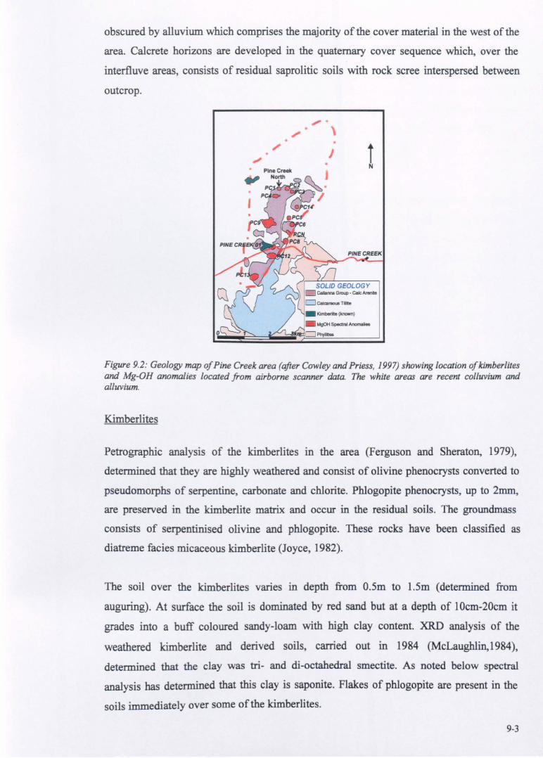
obscured by alluvium which comprises the majority of the cover material in the west of the

area. Calcrete horizons are developed in the quaternary cover sequence which, over the

interfluve areas, consists of residual saprolitic soils with rock scree interspersed between

outcrop.

" . " . , ) i

N

Figure 9.2: Geology map olPine Creek area (after Cowley and Priess, 1997) showing location olkimberlites and Mg-OH anomalies located from airborne scanner data. The white areas are recent colluvium and alluvium.

Kimberlites

Petrographic analysis of the kimberlites in the area (Ferguson and Sheraton, 1979),

determined that they are highly weathered and consist of olivine phenocrysts converted to

pseudomorphs of serpentine, carbonate and chlorite. Phlogopite phenocrysts, up to 2mm,

are preserved in the kimberlite matrix and occur in the residual soils. The groundmass

consists of serpentinised olivine and phlogopite. These rocks have been classified as

diatreme facies micaceous kimberlite (Joyce, 1982).

The soil over the kimberlites varies in depth from O.5m to 1.5m (determined from

auguring). At surface the soil is dominated by red sand but at a depth of lOcm-20cm it

grades into a buff coloured sandy-loam with high clay content. XRD analysis of the

weathered kimberlite and derived soils, carried out in 1984 (McLaughlin, 1 984),

determined that the clay was tri- and di-octahedral smectite. As noted below spectral

analysis has determined that this clay is saponite. Flakes of phlogopite are present in the

soils immediately over some of the kimberlites.

9-3

The laraest kimberlite in the rqion. Pine Creek 0 I. is located in a flat area on the southern

side of a shallow valle)" U.e aroWld rises 10 the south where outcrops of caJc-llel\itel

«&llana Group) occur, 'Ibere an: small outcrops ofthele sediments within the boundary of

the kimberlite, These rocks 1M)' be xmolithl of country rock in the kimberlite or faulted

blocks but iftJufficient exposure and lad of borehole infonnation exiltS to verify this.

9,3 FIELD STUDIES

My invettiptiOfti into the spectral retpOnIet in this IUU have included studies usina both

the GI~R IRJS MklV and PIMA 1J)CCU'OIIlCtCn. The most recent ofthete investiptions wu

completed in February 1998 utina • PIMA after the area Md been surveyed with the

HyMap 1CaMeI'. This study includet not only investiptionJ into the main kimberlite Pine

Creek 01 (FilW'C 9.2) but allO. number ofMI-OH anomalies which are now coftJidered to

be previousl), undiscovered kimberlite •.

The aims oflbete lpec1tal investiptions have been to:

• l>et.ennine the .pec1tal lipatwe of kimberlitc in the ilia.

• Ddmnine the spec1tal retponlC of the IOU derived from the kimberlite. • Ddennine the spectral responIC of lichen encrusted IOU •. • Map the ex1ent of the Ma-OH .iptW'C in the IOU. apinst the blckpund

.pectral response,

'Tbete studies have mainly been canicd out over the Pine Creek 0 I kimberlite but spec1tal

data were collected &om arlds covertna two other Ma"()H taIptI derived from the HyMap

data (f'lwe 9.2). Thete data are dilCUllOd in the Met jon on proceIIina of the ByMap data

below.

SlIdJl Ita .. of Jbc Kimber"l4!

'1bcre are no outaopl of kimberlite (Fiaure 1. 1) in the ..... thouah OCCMionaJ pieces of

nc.t of WCIdhered kimberlite ocxw. Put exploration acdvity in the area has resulted in

palC.hes of kimberlite .poll ocxurrina at the surfllCe cooslttina of I arey da), matrix in

which nodules of WCIdhered ICI"pCfttinitOd kimberlite and Raket of phloaopite are

abundant. Spec:trI that I have rec:onted with the PIMA from thiny samples of this

WCIdhered kimberlite all produced • IpOCtrum that i, typifted by that ahown in Flpre 9.3.

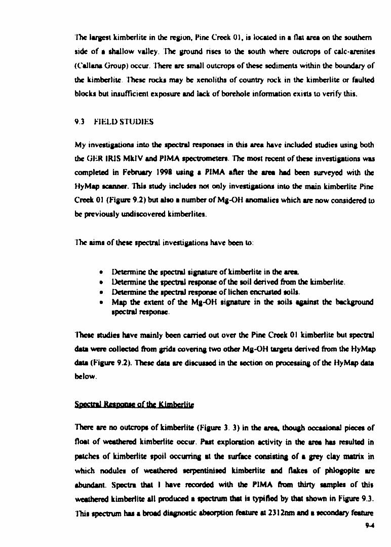
Ibis apectnam has • broed diapottic abIorpdon fealW'e II 231lnm and lleCOndary feabft ,....

at 2386nm; whilst this spectrum lacks other minor features, it can be interpreted as a

generic kimberlite spectrum that results from the mixture of several phyllosilicate minerals

including talc, serpentine, phlogopite and saponite. There is no indication of the presence

of chlorite in any spectra of the kimberlite spoil though it is mentioned in the petrographic

description of the rock (Joyce, 1982). XRD analysis of this material (McLaughlin, 1984)

determined that it comprised mainly of trl-octahedral smectite. Analysis of the spectra

indicates that the smectite is saponite and the deep featureless water absorption features at

1400nm and 1900nm support the identification of smectite by XRD.

Figure 9.3: Average spectra (hull quotient transformed) of Pine Creek 01 kimberlite. Vertical bars at 2312nm and 2386nmfor reference.

Spectral Response of Soil derived from Kimberlite

Spectra were recorded at 15cm intervals for soil samples obtained from an augur hole in

the eastern arm of the Pine Creek 01 kimberlite (grid station 1200/1] 50, Figure 9.4). These

spectra are presented in Figure 9.5, which shows that there is variation in the spectra and,

therefore, mineralogy of the soil derived from the kimberlite. The surface material is red

brown sandy loam that changes to a buff to yellow clay rich soil at a depth of around

20cm.

9-5

~ ~

u KIMBERLITE

... ANCS~ONE OUTC~OP

o I

1DO

SPECTRAL GRID

/ , I

200

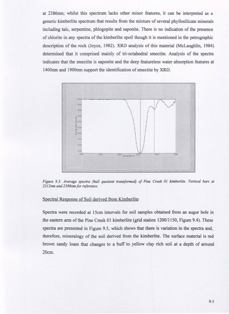
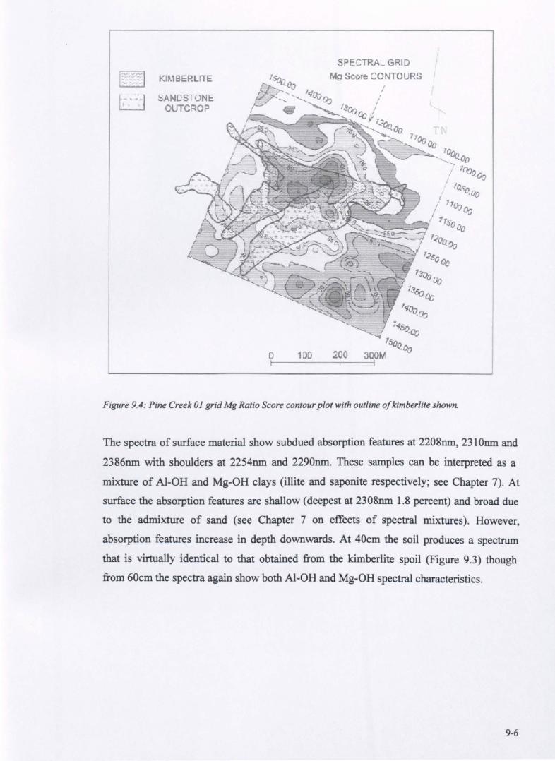
Figure 9.4: Pine Creek 01 grid Mg Ratio Score contour plot with outline of kimberlite shown

The spectra of surface material show subdued absorption features at 2208nm, 231 Onm and

2386nm with shoulders at 2254nm and 2290nm. These samples can be interpreted as a

mixture of AI-OH and Mg-OH clays (illite and saponite respectively; see Chapter 7). At

surface the absorption features are shallow (deepest at 2308nm 1.8 percent) and broad due

to the admixture of sand (see Chapter 7 on effects of spectral mixtures). However,

absorption features increase in depth downwards. At 40cm the soil produces a spectrum

that is virtually identical to that obtained from the kimberlite spoil (Figure 9.3) though

from 60cm the spectra again show both Al-OH and Mg-OH spectral characteristics.

9-6

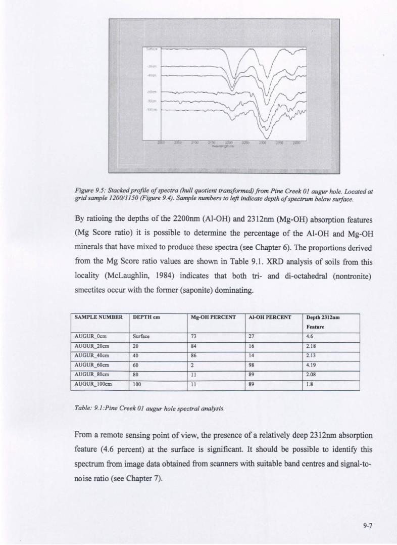
Figure 9.5: Stacked profile of spectra (hull quotient transformed) from Pine Creek OJ augur hole. Located at grid sample J 20011150 (Figure 9.4). Sample numbers to left indicate depth of spectrum below surface.

By ratioing the depths of the 2200nm (Al-OH) and 2312nm (Mg-OH) absorption features

(Mg Score ratio) it is possible to determine the percentage of the Al-OH and Mg-OH

minerals that have mixed to produce these spectra (see Chapter 6). The proportions derived

from the Mg Score ratio values are shown in Table 9.1. XRD analysis of soils from this

locality (McLaughlin, 1984) indicates that both tri- and di-octahedral (nontronite)

smectites occur with the former (saponite) dominating.

SAMPLE NUMBER DEPTHc:m ME-OH PERCENT AI-OH PERCENT Depth 13t:znm

Feature

AUGUR_Oem Surface 73 27 4.6

AUGUR_20cm 20 84 16 2.18

AUGUR_40cm 40 86 14 2.13

AUGUR_60em 60 2 98 4.19

AUGUR_80em 80 11 89 2.08

AUGUR_IOOcm 100 II 89 1.8

Table: 9. J :Pine Creek 01 augur hole spectral analysis.

From a remote sensing point of view, the presence ofa relatively deep 2312nm absorption

feature (4.6 percent) at the surface is significant. It should be possible to identify this

spectrum from image data obtained from scanners with suitable band centres and signal-to­

noise ratio (see Chapter 7).

9-7

Surface Spectral Mapping

Field work employed a new version of the PIMA, the PIMA RAP spectrometer, to collect

spectra which were recorded at regular grid stations by digging down 20cms and placing

the instrument on the spoil. These data were processed by focusing on the 2000nm-

2500nm wavelength range and after smoothing and applying a hull quotient transform,

determining the Mg Score ratio. The Surfer package was used to contour these Mg Score

values.

Pine Creek 01 Kimberlite

A 500m by 600m grid covers the Pine Creek 01 kimberlite as well as the majority of an

Mg-OH anomaly which is located to the south east and that was detected from the HyMap

scanner data.

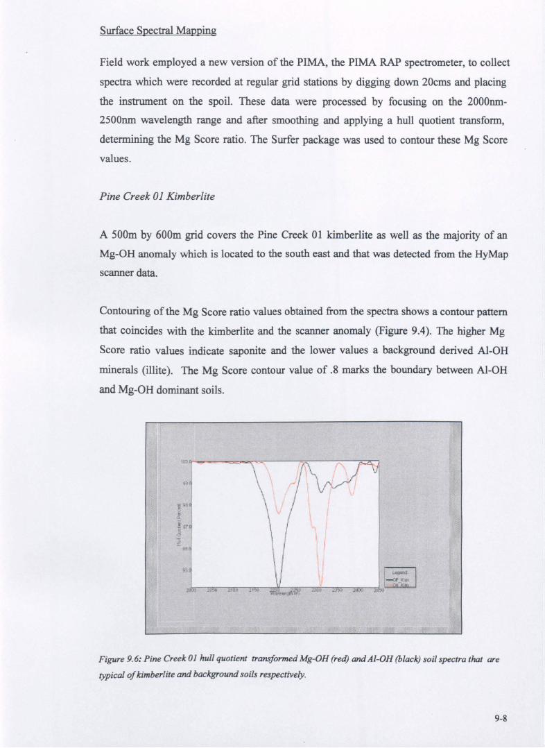
Contouring of the Mg Score ratio values obtained from the spectra shows a contour pattern

that coincides with the kimberlite and the scanner anomaly (Figure 9.4). The higher Mg

Score ratio values indicate saponite and the lower values a background derived Al-OH

minerals (illite). The Mg Score contour value of .8 marks the boundary between Al-OH

and Mg-OH dominant soils.

Figure 9.6: Pine Creek 01 hull quotient transformed Mg-OH (red) and AI-OH (black) soil spectra that are

typical of kimberlite and background soils respectively.

9-8

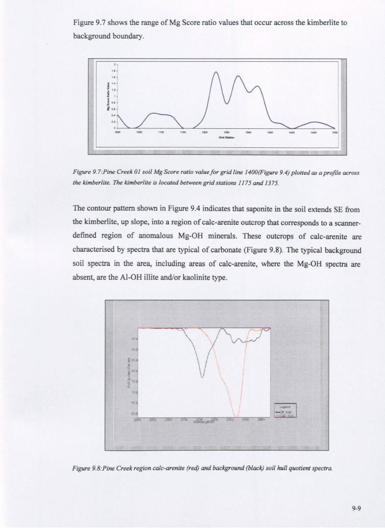
Figure 9.7 shows the range of Mg Score ratio values that occur across the kimberlite to

background boundary.

1.'

! .. .. > 1.2

! 1

j o. 1 0 .•

1000 ,oeo 1100 1150 "'50 '''0 '500

Figure 9.7:Pine Creek 01 soil MgScore ratio value/or grid line 1400(Figure 9.4) plotted as aproji/e across

the kimberlite. The kimberlite is located between grid stations 1175 and 13 75.

The contour pattern shown in Figure 9.4 indicates that saponite in the soil extends SE from

the kimberlite, up slope, into a region of calc-arenite outcrop that corresponds to a scanner­

defined region of anomalous Mg-OH minerals. These outcrops of calc-arenite are

characterised by spectra that are typical of carbonate (Figure 9.8). The typical background

soil spectra in the area, including areas of calc-arenite, where the Mg-OH spectra are

absent, are the Al-OH illite and/or kaolinite type.

Figure 9.8:Pine Creek region calc-arenite (red) and background (black) soil hull quotient spectra.

9-9

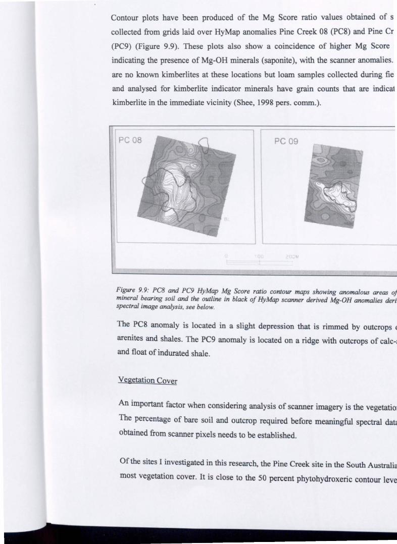
Contour plots have been produced of the Mg Score ratio values obtained of s

collected from grids laid over HyMap anomalies Pine Cre~k 08 (PC8) and Pine Cr

(PC9) (Figure 9.9). These plots also show a coincidence of higher Mg Score

indicating the presence of Mg-OH minerals (saponite), with the scanner anomalies.

are no known kimberlites at these locations but loam samples collected during fie

and analysed for kimberlite indicator minerals have grain counts that are indica1

kimberlite in the immediate vicinity (Shee, 1998 pers. comm.).

pe08 PC 09

L

Figure 9.9: PCB and PC9 HyMap Mg Score ratio contour maps shOWing anomalous areas of mineral bearing soil and the outline in black of HyMap scanner derived Mg-OH anomalies dern spectral image analysis, see below.

The PC8 anomaly is located in a slight depression that is rimmed by outcrops 0

arenites and shales. The PC9 anomaly is located on a ridge with outcrops of calC-2

and float of indurated shale.

Vegetation Cover

An important factor when considering analysis of scanner imagery is the vegetation

The percentage of bare soil and outcrop required before meaningful spectral data

obtained from scanner pixels needs to be established.

Of the sites I investigated in this research, the Pine Creek site in the South Australia '

most vegetation cover. It is close to the 50 percent phytohydroxeric contour level

3.1). On occasions it receives heavy rainfall that results in rapid ephemeral vegetation

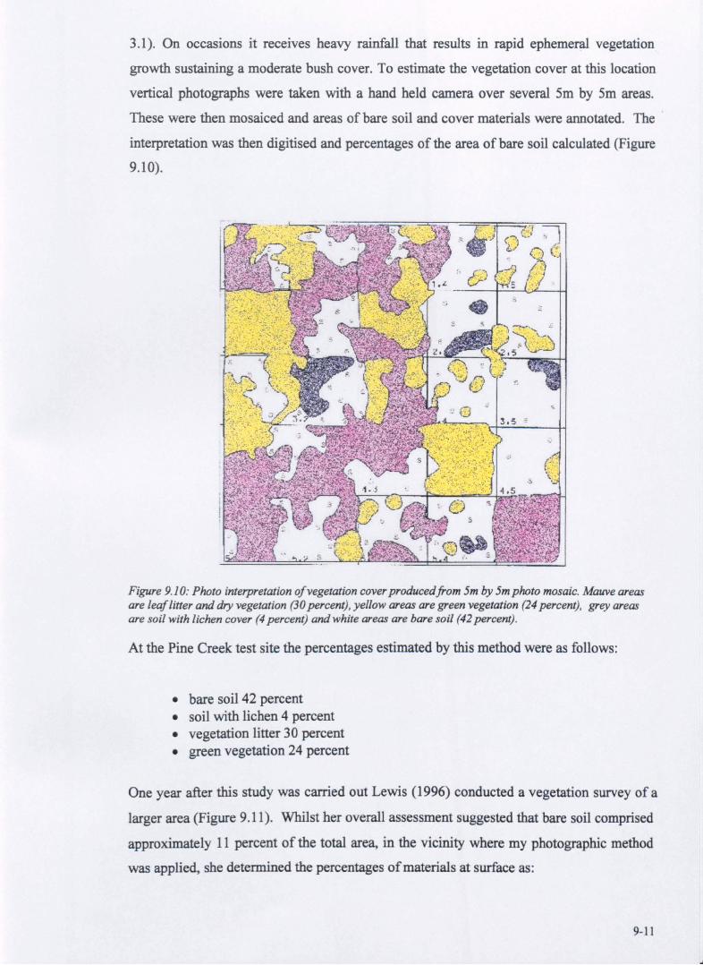
growth sustaining a moderate bush cover. To estimate the vegetation cover at this location

vertical photographs were taken with a hand held camera over several 5m by 5m areas.

These were then mosaiced and areas of bare soil and cover materials were annotated. The

interpretation was then digitised and percentages of the area of bare soil calculated (Figure

9.10).

Figure 9.10: Photo interpretation of vegetation cover producedfrom 5m by 5m photo mosaic. Mauve areas are leaf litter and dry vegetation (30 percent), yellow areas are green vegetation (24 percent), grey areas are soil with lichen cover (4 percent) and white areas are bare soil (42 percent) .

At the Pine Creek test site the percentages estimated by this method were as follows:

• bare soil 42 percent • soil with lichen 4 percent • vegetation litter 30 percent • green vegetation 24 percent

One year after this study was carried out Lewis (1996) conducted a vegetation survey of a

larger area (Figure 9.11). Whilst her overall assessment suggested that bare soil comprised

approximately 11 percent of the total area, in the vicinity where my photographic method

was applied, she determined the percentages of materials at surface as:

9-11

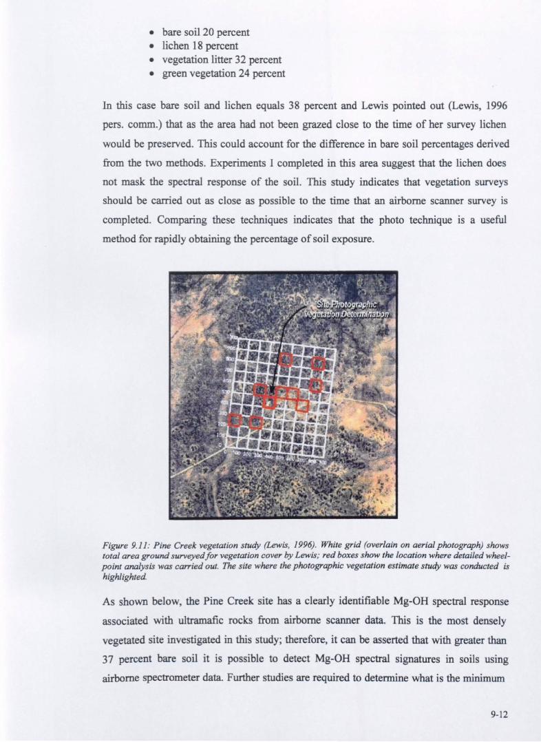
• bare soil 20 percent • lichen 18 percent • vegetation litter 32 percent • green vegetation 24 percent

In this case bare soil and lichen equals 38 percent and Lewis pointed out (Lewis, 1996

pers. comm.) that as the area had not been grazed close to the time of her survey lichen

would be preserved. This could account for the difference in bare soil percentages derived

from the two methods. Experiments I completed in this area suggest that the lichen does

not mask the spectral response of the soil. 1bis study indicates that vegetation surveys

should be carried out as close as possible to the time that an airborne scanner survey is

completed. Comparing these techniques indicates that the photo technique is a useful

method for rapidly obtaining the percentage of soil exposure.

Figure 9.11: Pine Creek vegetation study (Lewis, 1996). White grid (overlain on aerial photograph) shows total area ground surveyed for vegetation cover by Lewis; red boxes show the location where detailed whee/­point analysis was carried out. The site where the photographic vegetation estimate study was conducted is highlighted

As shown below, the Pine Creek site has a clearly identifiable Mg-OH spectral response

associated with ultramafic rocks from airborne scanner data. This is the most densely

vegetated site investigated in this study; therefore, it can be asserted that with greater than

37 percent bare soil it is possible to detect Mg-OH spectral signatures in soils using

airborne spectrometer data. Further studies are required to determine what is the minimum

9-12

soil exposure that precludes useful geological data being acquired from airborne scanner

unagery.

Spectral Effects of Lichen

As Lewis (1996) has pointed out lichen can cover up to twenty six percent of the ground in

this region. As lichen or algal encrustations are in effect dry vegetation, they have spectra

with absorption features near 2300nm which could be a limiting factor in obtaining

geologically meaningful information from scanner data in this region. Therefore, spectra

were recorded from patches of lichen and adjacent soil (in the field) by placing the PIMA

onto the surface and ensuring that it did not disturb the lichen crust. There are two types of

lichen seen in the region; a black crust that is ubiquitous and termed by Lewis (1996)

'hlgal crust" rather than lichen senso stricto and true white lichen. The white lichen is far

less prevalent and usually occurs close to bushes and shrubs.

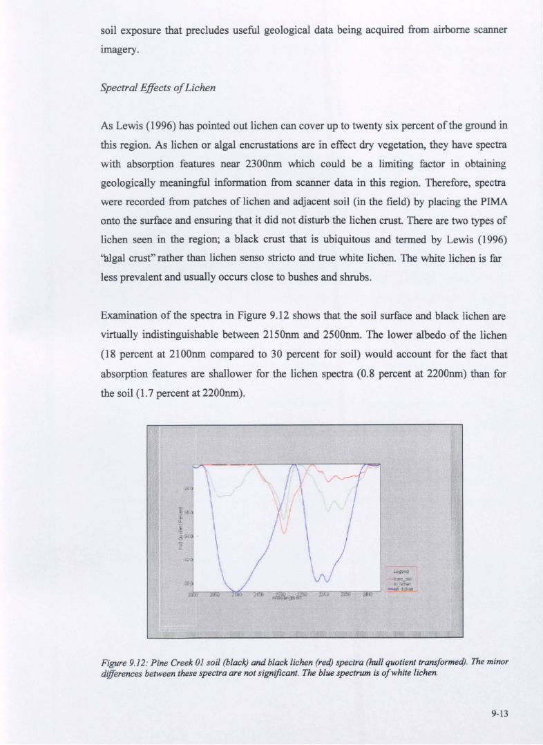
Examination of the spectra in Figure 9.12 shows that the soil surface and black lichen are

virtually indistinguishable between 2150nm and 2500nm. The lower albedo of the lichen

(18 percent at 2100nm compared to 30 percent for soil) would account for the fact that

absorption features are shallower for the lichen spectra (0.8 percent at 2200nm) than for

the soil (1.7 percent at 2200nm).

bOft ..... b ~

~~=-~~~~~-,~~~~r-~~ -WI

Figure 9.12: Pine Creek OJ soil (black) and black lichen (red) spectra (hull quotient transformed). The minor differences between these spectra are not significant. The blue spectrum is of white lichen.

9-13

This check was carried out on background soils, not over the kimberlite. The soil and

lichen spectra both represent poorly ordered kaolinite, with a weak 2168nm shoulder,

2208nm main absorption features and minor absorptions at 2312nm and 2340nm. It

confirms my visual inspection in the field, supported by Lewis (1996 pers. comm) that the

black lichen-algal crust consists of a matrix of soil bound together by the algae, which

explains why the soil dominates its spectra. The white lichen has definite cellulose

absorption features in its spectrum (see Chapter 6) with a broad deep absorption (4 percent)

at 2100nm and 230Onm. The near 2100nm absorption feature is seen in the black lichen

spectra confirming the presence of organic material.

Since the white lichen is not widespread in the area and often occurs in the shadow area of

shrubs, it is doubtful that it would cause confusion in interpreting scanner imagery. The

widespread black encrustation appears to reduce the soil albedo and, therefore, spectral

contrast. However, it does not eliminate diagnostic spectral features. Other vegetation such

as trees, shrubs and litter obscure the surface and, therefore, geological signatures, but they

can be identified in the imagery.

9.4 GROUND BASED SPECTRAL ANALYSIS OF KIMBERLITE AND BACKGROUND SOILS FROM PINE CREEK USING THE GEOSCAN MK II SCANNER

In 1992 Dr Frank Honey (founder of the GEOSCAN Company) suggested the idea of

collecting spectra with the GEOSCAN MkII scanner on the ground. However, he pointed

out that there was a problem in extracting a spectral signature from GEOSCAN MkII

imagery at the time due to the gain and offsets introduced into the data during data

collection. Dr Honey suggested, that dark and light reference plates could be measured

together with the sample. With software developed to use the reference readings to correct

data collected to reflectance such an experiment would be worthwhile.

An experiment was set-up to determine if data from the GEOSCAN MkII scanner could be

used to discriminate between soil derived from kimberlite (Mg-OH mineral rich) and

background soils (Al-OH mineral rich). In this experiment only the SWIR2 channels are

evaluated (200Onm-235Onm).

9-14

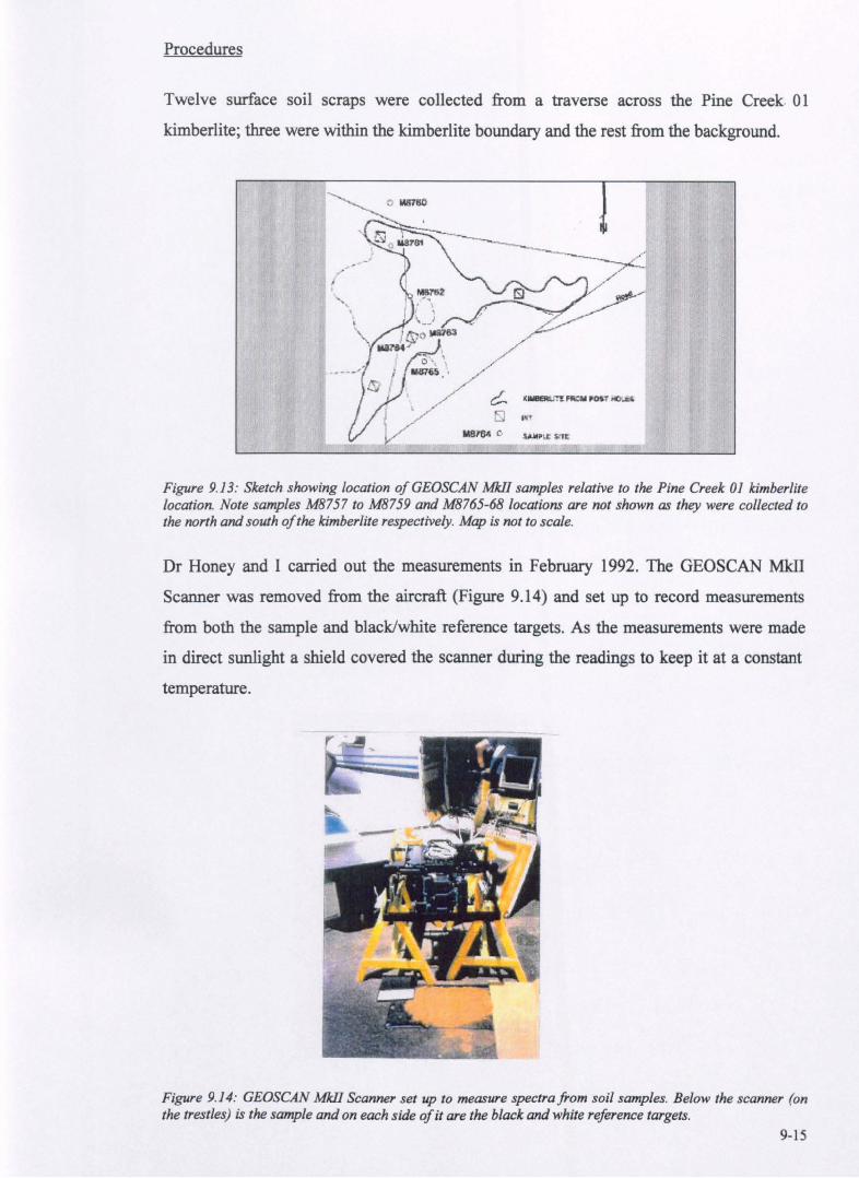
Procedures

Twelve surface soil scraps were collected from a traverse across the Pine Creek. 01

kimberlite; three were within the kimberlite boundary and the rest from the background.

Figure 9.13: Slcetch showing location ofGEOSCAN MkI1 samples relative to the Pine Creek 01 kimberlite location. Note samples M8757 to M8759 and MB765-68 locations are not shown as they were collected to the north and south of the kimberlite respectively. Map is not to scale.

Dr Honey and I carried out the measurements in February 1992. The GEOSCAN MkII

Scanner was removed from the aircraft (Figure 9.14) and set up to record measurements

from both the sample and black/white reference targets. As the measurements were made

in direct sunlight a shield covered the scanner during the readings to keep it at a constant

temperature.

Figure 9.14: GEOSCAN MkI1 Scanner set up to measure spectra from soil samples. Below the scanner (on the trestles) is the sample and on each side of it are the black and white reference targets.

9-15

The data were recorded as 768 pixel by 256 line images; the central portion of each image

was sample material and about 30 pixels at the end of each line the reference targets.

The electrical engineer responsible for development of this instrument (N. Adronis)

provided equations, which allowed the gain and offsets to be removed from the data. These

equations were supplied to Dr A Becker who wrote a program (Appendix 4) that was used

in conjunction with the average of the dark target reference values to convert the samples

to radiance readings in watts per centimetre squared.

Images were then constructed by processing the raw data with this program. These

radiance images were then processed using the log residual program to remove the solar

background curve and produce pseudo-reflectance images, in effect a hull quotient

transform of the data. The log residual transform was carried out using the version

developed to run with the eS S600 system software.

Each sample also had its SWIR spectra measured with the PIMA spectrometer and these

were plotted as follows:

Analysis

• Standard spectra • Hull quotient spectra. • Convolved spectra - spectra convolved to GEOSCAN MIdI

wavelengths.

Visual analysis of the various spectra, shown in Figures 9.15 to 9.19 was undertaken and is

reported on below.

9-16

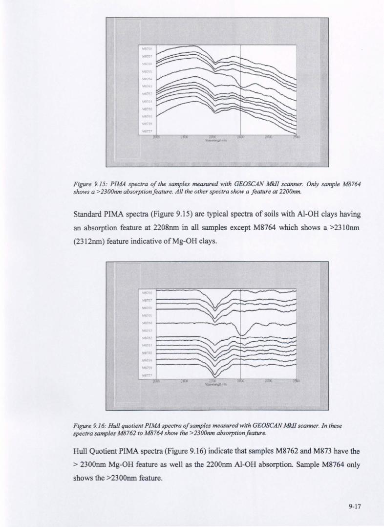
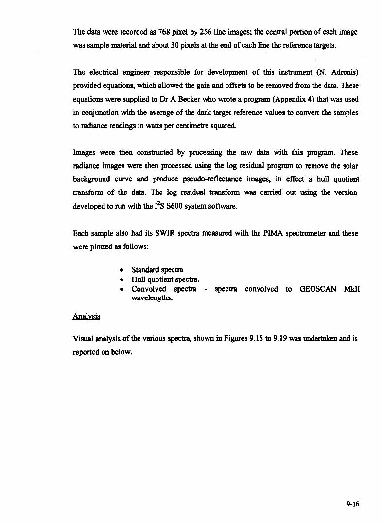
Figure 9.15: PIMA spectra of the samples measured with GEOSCAN MkIJ scanner. Only sample M8764 shows a >2300nm absorptionfeature. All the other spectra show a feature at 2200nm.

Standard PIMA spectra (Figure 9.15) are typical spectra of soils with AI-OR clays having

an absorption feature at 2208nm in all samples except M8764 which shows a >2310nm

(2312nm) feature indicative of Mg-OH clays.

Figwe 9.16: Hull quotient PIMA spectra of samples measured with GEOSCAN MkIJ scanner. In these spectra samples M8762 to M8764 show the> 2300nm absorption feature.

Hull Quotient PIMA spectra (Figure 9.16) indicate that samples M8762 and M873 have the

> 2300nm Mg-OH feature as well as the 2200nm Al-OH absorption. Sample M8764 only

shows the >2300nm feature.

9-17

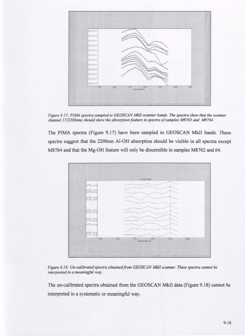
Figure 9.17: PIMA spectra sampled to GEOSCAN MIdI scanner bands. The spectra show that the scanner channel 17(2300nm) should show the absorption/eature in spectra o/samples M8763 and M8764.

The PIMA spectra (Figure 9.17) have been sampled to GEOSCAN MklI bands. These

spectra suggest that the 2200nm Al-OH absorption should be visible in all spectra except

M8764 and that the Mg-OH feature will only be discernible in samples M8762 and 64.

---' - -- -:: -

-----.. "..- ... --.

.--

Figure 9.18: Un-calibrated spectra obtained from GEOSCAN MkIJ scanner. These spectra cannot be interpreted in a meaningful way.

The un-calibrated spectra obtained from the GEOSCAN MklI data (Figure 9.18) cannot be

interpreted in a systematic or meaningful way.

9-18

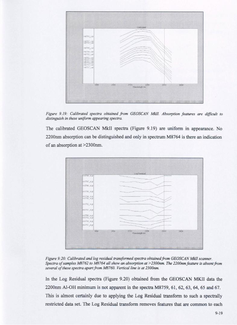
Figure 9.19: Calibrated spectra obtained from GEOSCAN Mkll. Absorption features are difficult to distinguish in these uniform appearing spectra.

The calibrated GEOSCAN Mkll spectra (Figure 9.19) are uniform in appearance. No

2200nm absorption can be distinguished and only in spectrum M8764 is there an indication

of an absorption at >2300nm.

Figure 9:20: Calibrated and log residual transformed spectra obtainedfrom GEOSCAN MkII scanner. Spectra of samples M8762 to M8764 all show an absorption at >2300nm. The 2200nmfeature is absentfrom several of these spectra apart from M8760. Vertical line is at 2300nm.

In the Log Residual spectra (Figure 9.20) obtained from the GEOSCAN MKlI data the

2200nm Al-OH minimum is not apparent in the spectra M8759, 61, 62, 63, 64, 65 and 67.

This is almost certainly due to applying the Log Residual transform to such a spectrally

restricted data set. The Log Residual transform removes features that are common to each

9-19

pixel, in this case it is removing the ubiquitous 2200nm feature. However, the convolved

PIMA spectra (Figure 9.17) indicate that it should be obvious in all of the spectra except

M8764. Samples M8762-M8764 all show a minimum at >2300nm that indicates

absorption due to the presence of Mg-OH minerals

Comments and Conclusions

This investigation confirms that the GEOSCAN MkI1 scanner could, under favourable

conditions, with corrections made for atmosphere and gain and offset, detect and

differentiate between kimberlite derived soils and those from background Al-OH rich

lithologies.

This study was carried out to investigate whether the GEOSCAN MkII had potential to

locate Mg-OH bearing rocks and the soils derived from them. In Chapter 11 it is shown

that the noise level in GEOSCAN MkII data, when acquired operationally during an

airborne survey, can reduce the potential discrimination that this study suggests is possible.

As shown in Chapter 7 noise can significantly reduce the discrimination possible with

scanner data. Prior to this study, the noise level in operationally acquired GEOSCAN data

was estimated to be around 220: 1 (Hook, 1990). In the configuration used to acquire these

static test data, the signal-to-noise level would have been higher than during airborne

operations as induced electronic noise and vibration would have been less (Honey, 1992

pers. comm.).

Dr Honey has recently recommissioned the GEOSCAN MkII scanner. He has modified

this scanner to collect data in integer rather than byte format thus eliminating the problems

with gain and offset corrections mentioned above. Dr Honey claims (pers. comm) to have

improved the SNR by a factor of two or three (400: 1 ?). Therefore, in future this instrument

may be able to acquire operationally useful data for the detection of out-cropping and

weathered ultramafic rocks.

9.S IMAGE PROCESSING OF HyMap SCANNER DATA

Conventional Processina

According to the manufacturer (Cocks, 1997 pers. comm.) the signal-to-noise ratio for the

HyMap scanner used in this study exceeds 600:1 in the SWIR2 spectral region. It should

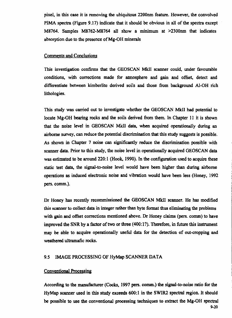
be possible to use the conventional processing techniques to extract the Mg-OH spectral 9-20

signature as described in Chapter 8. To validate this the following processes have been

applied to the data:

• Colour composite images from raw data. • Colour composites oflog residual transformed images. • Band ratio. • Crosta principal component transform (Crosta technique). • Anomaly residual band prediction.

These processes have been applied with consideration to the band centre wavelengths for

this imagery shown in Table 9.2.

SWIRl BAND WAVELENGTH SWIlUBAND WAVELENGTH

DDI om

1 2087 17 2267

2 2099 18 2278

3 2111 19 2288

4 2123 20 2298

5 2135 21 2308

6 2147 22 2318

7 2158 23 2328

8 2170 24 2337

9 2181 25 2347

10 2192 26 2356

11 2203 27 2366

12 2214 28 237S

13 2225 29 2384

14 2236 30 2393

15 2246 31 2402

16 22S7 32 2411

Table 9.2: HyMap SWIR2 band centres in nm.

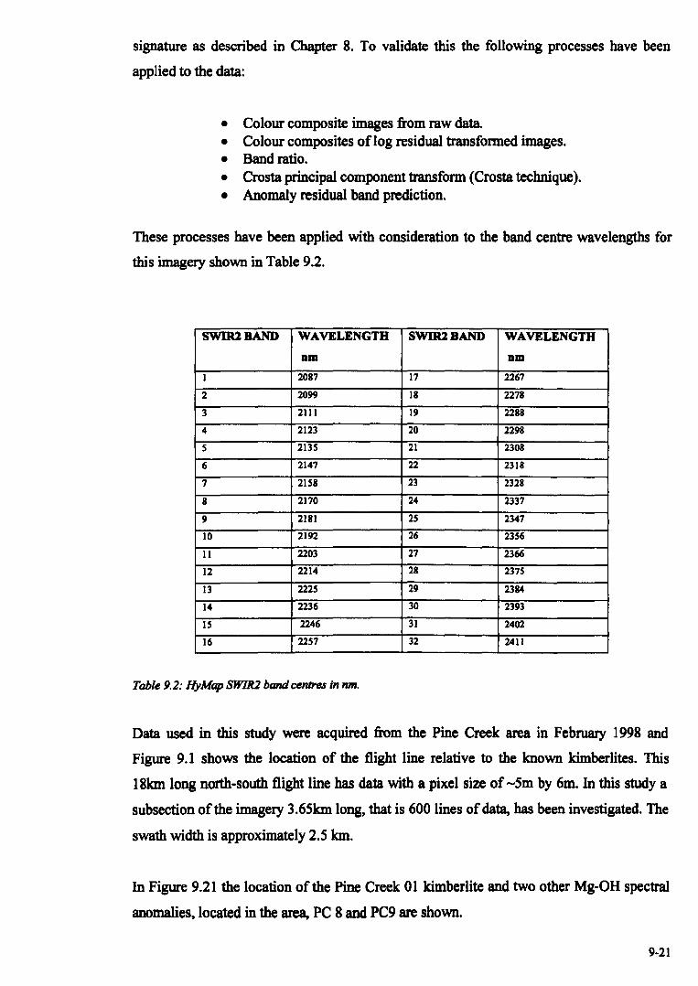
Data used in this study were acquired from the Pine Creek area in February 1998 and

Figure 9.1 shows the location of the flight line relative to the known kimberlites. This

18lan long north-south flight line has data with a pixel size of -Sm by 6m. In this study a

subsection of the imagery 3.6Slan long, that is 600 lines of data, has been investigated. The

swath width is approximately 2.S lan.

In Figure 9.21 the location of the Pine Creek 01 kimberlite and two other Mg-OH spectral

anomalies, located in the area, PC 8 and PC9 are shown.

9-21

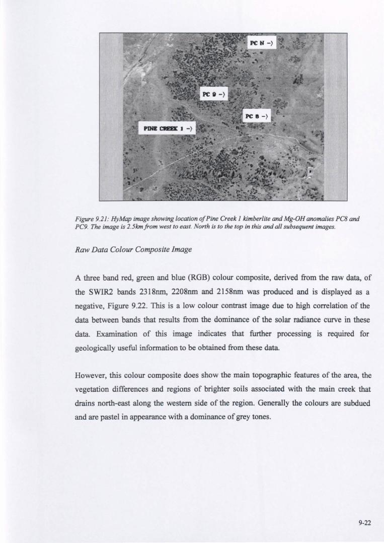
Figure 9.21: HyMap image showing location o/Pine Creek 1 kimberlite and Mg-OH anomalies PCB and PC9. The image is 2.5lcmfrom west to east. North is to the top in this and all subsequent images.

Raw Data Colour Composite Image

A three band red, green and blue (RGB) colour composite, derived from the raw data, of

the SWIR2 bands 2318nm, 2208nm and 2158nm was produced and is displayed as a

negative, Figure 9.22. This is a low colour contrast image due to high correlation of the

data between bands that results from the dominance of the solar radiance curve in these

data. Examination of this image indicates that further processing is required for

geologically useful information to be obtained from these data.

However, this colour composite does show the main topographic features of the area, the

vegetation differences and regions of brighter soils associated with the main creek that

drains north-east along the western side of the region. Generally the colours are subdued

and are pastel in appearance with a dominance of grey tones.

9-22

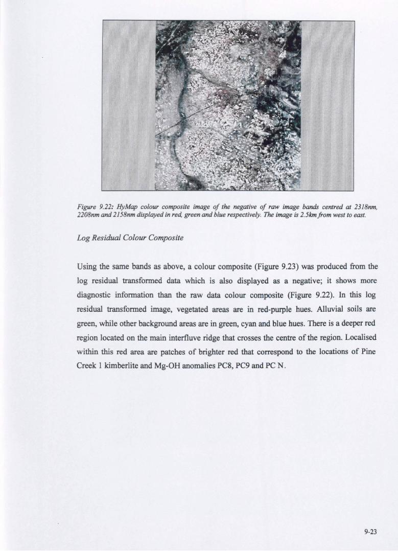
Figure 9.22: HyMap colour composite image of the negative of raw image bands centred at 2318nm, 2208nm and 21 58nm displayed in red, green and blue respectively. The image is 2.5kmfrom west to east.

Log Residual Colour Composite

Using the same bands as above, a colour composite (Figure 9.23) was produced from the

log residual transformed data which is also displayed as a negative; it shows more

diagnostic information than the raw data colour composite (Figure 9.22). In this log

residual transformed image, vegetated areas are in red-purple hues. Alluvial soils are

green, while other background areas are in green, cyan and blue hues. There is a deeper red

region located on the main interfluve ridge that crosses the centre of the region. Localised

within this red area are patches of brighter red that correspond to the locations of Pine

Creek I kimberlite and Mg-OH anomalies PC8, PC9 and PC N.

9-23

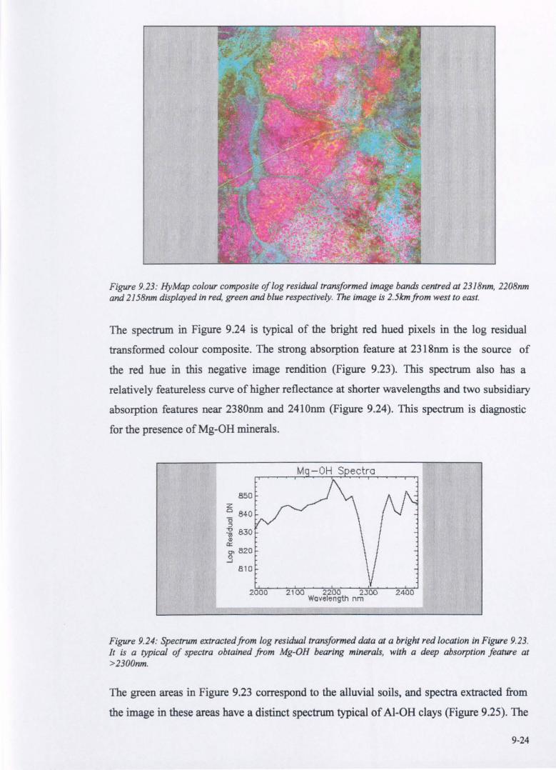
Figure 9.23: HyMap colour composite of log residual transformed image bands centred at 231Bnm, 220Bnm and 215Bnm displayed in red, green and blue respectively. The image is 2.5lcmfrom west to east.

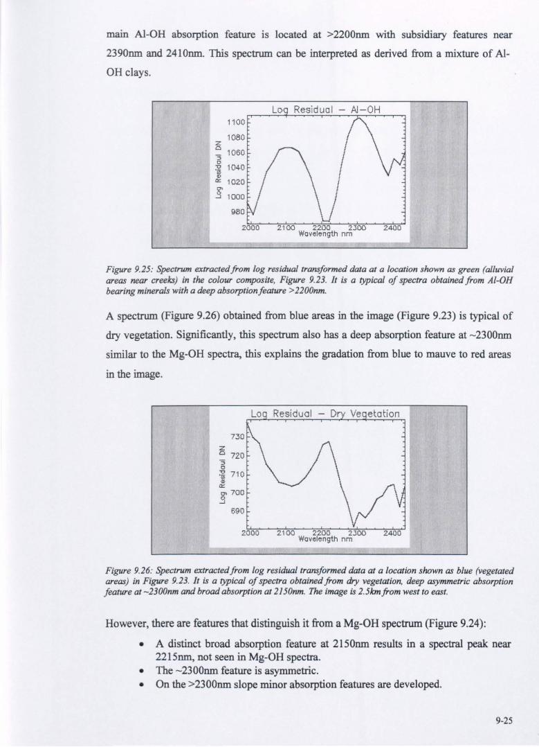
The spectrum in Figure 9.24 is typical of the bright red hued pixels in the log residual

transformed colour composite. The strong absorption feature at 2318nm is the source of

the red hue in this negative image rendition (Figure 9.23). This spectrum also has a

relatively featureless curve of higher reflectance at shorter wavelengths and two subsidiary

absorption features near 2380nm and 2410nm (Figure 9.24). This spectrum is diagnostic

for the presence of Mg-OH minerals.

850 z o 840 "0 :::J

~ 830 ~

a:: 8' 820

...:J

810

Figure 9.24: Spectrum extractedfrom log residual transformed data at a bright red location in Figure 9.23. It is a typical of spectra obtained from Mg-OH bearing minerals, with a deep absorption feature at >2300nm.

The green areas in Figure 9.23 correspond to the alluvial soils, and spectra extracted from

the image in these areas have a distinct spectrum typical of Al-OH clays (Figure 9.25). The

9-24

mam Al-OH absorption feature is located at >2200nm with subsidiary features near

2390nm and 2410nm. This spectrum can be interpreted as derived from a mixture of Al­

OH clays.

Lo Residual - A1-0H 1100

1080 z a

1060 :; 0

-0 1040 ' i,? I)

a:: 1020 0>

.9 1000

980

2000

Figure 9.25: Spectrum extractedfrom log residual transformed data at a location shown as green (alluvial areas near creeks) in the colour composite, Figure 9.23. It is a typical of spectra obtained from AI-OR bearing minerals with a deep absorption feature > 2200nm.

A spectrum (Figure 9.26) obtained from blue areas in the image (Figure 9.23) is typical of

dry vegetation. Significantly, this spectrum also has a deep absorption feature at - 2300nm

similar to the Mg-OH spectra, this explains the gradation from blue to mauve to red areas

in the image.

730

z a 720 :; o l 710 a:: 8' 700

...:J

690

Figure 9.26: Spectrum extractedfrom log residual transformed data at a location shown as blue (vegetated areas) in Figure 9.23. It is a typical of spectra obtained from dry vegetation, deep asymmetric absorption feature at - 2300nm and broad absorption at 2150nm. The image is 2. 5km from west to east.

However, there are features that distinguish it from a Mg-OH spectrum (Figure 9.24):

• A distinct broad absorption feature at 2150nm results in a spectral peak near 221Snm, not seen in Mg-OH spectra.

• The - 2300nm feature is asymmetric. • On the >2300nm slope minor absorption features are developed.

9-25

However, in the colour composite this spectral type results in confusion between Mg-OH

minerals and dry vegetation (mauve-red hues).

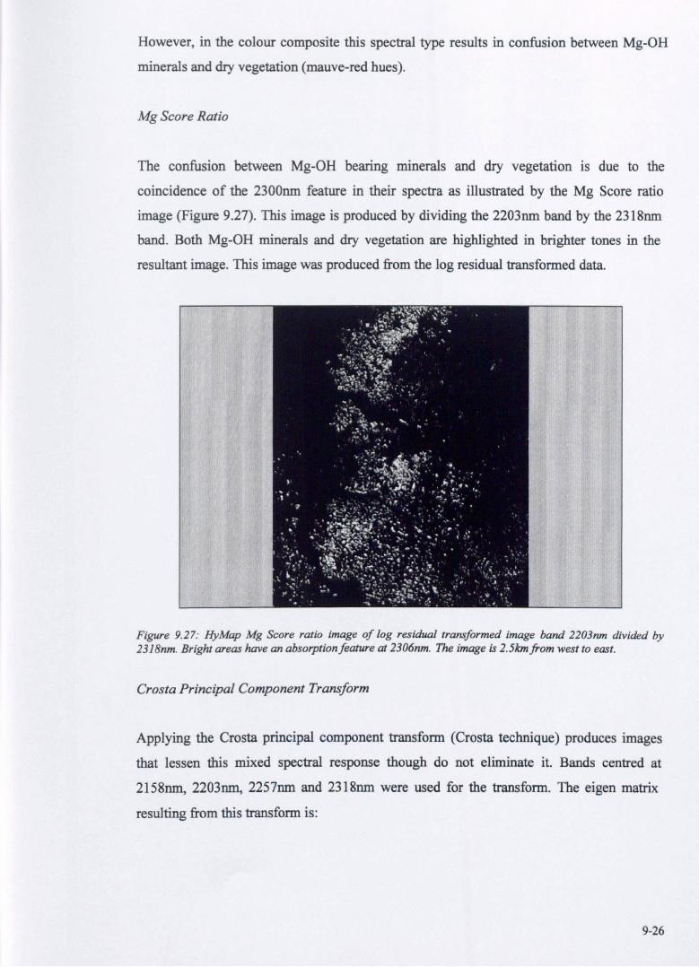
Mg Score Ratio

The confusion between Mg-OH bearing minerals and dry vegetation is due to the

coincidence of the 2300nm feature in their spectra as illustrated by the Mg Score ratio

image (Figure 9.27). This image is produced by dividing the 2203nm band by the 2318nm

band. Both Mg-OH minerals and dry vegetation are highlighted in brighter tones in the

resultant image. This image was produced from the log residual transformed data.

Figure 9.27: HyMap Mg Score ratio image of log residual transformed image band 2203nm divided by 2318nm. Bright areas have an absorptionfeature at 2306nm. The image is 2.5kmfrom west to east.

Crosta Principal Component Transform

Applying the Crosta principal component transform (Crosta technique) produces images

that lessen this mixed spectral response though do not eliminate it. Bands centred at

2158nm, 2203nm, 2257nm and 2318nm were used for the transform. The eigen matrix

resulting from this transform is:

9-26

BAND 2158nm 2203nm 2257nm 2306nm

PCl 0.081 -0.280 -0.600 0.745

PC2 -0.381 - -0.433 -0.573 -0.583

PC3 0.590 - -0.548 0.532 0.279

PC4 0.707 - 0.659 0.197 -0.166

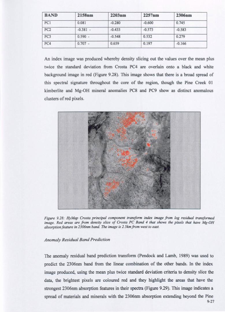
An index image was produced whereby density slicing out the values over the mean plus

twice the standard deviation from Crosta PC4 are overlain onto a black and white

background image in red (Figure 9.28). This image shows that there is a broad spread of

this spectral signature throughout the core of the region, though the Pine Creek 01

kimberlite and Mg-OH mineral anomalies PC8 and PC9 show as distinct anomalous

clusters of red pixels.

Figure 9.28: HyMap Crosta principal component transform index image from log residual transformed image. Red areas are from density slice of Crosta PC Band 4 that shows the pixels that have Mg-OH absorptionfeature in 2306nm band. The image is 2.5kmfrom west to east.

Anomaly Residual Band Prediction

The anomaly residual band prediction transform (pendock and Lamb, 1989) was used to

predict the 2306nm band from the linear combination of the other bands. In the index

image produced, using the mean plus twice standard deviation criteria to density slice the

data, the brightest pixels are coloured red and they highlight the areas that have the

strongest 2306nm absorption features in their spectra (Figure 9.29). This image indicates a

spread of materials and minerals with the 2306nm absorption extending beyond the Pine 9-27

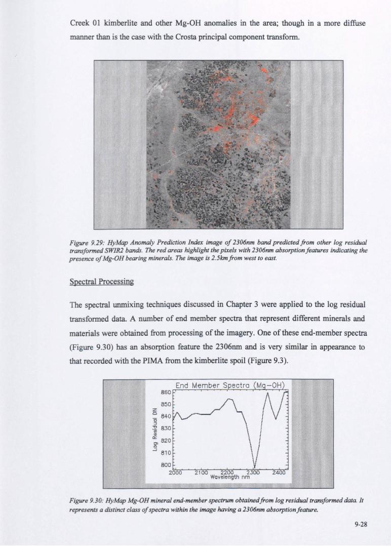
Creek 01 kimberlite and other Mg-OH anomalies in the area; though in a more diffuse

manner than is the case with the Crosta principal component transform.

Figure 9.29: HyMap Anomaly Prediction Index image of 2306nm band predicted from other log residual transformed SWIR2 bands. The red areas highlight the pixels with 2306nm absorption features indicating the presence of Mg-OH bearing minerals. The image is 2.5kmfrom west to east.

Spectral Processing

The spectral unmixing techniques discussed in Chapter 3 were applied to the log residual

transformed data. A number of end member spectra that represent different minerals and

materials were obtained from processing of the imagery. One of these end-member spectra

(Figure 9.30) has an absorption feature the 2306nm and is very similar in appearance to

that recorded with the PIMA from the kimberlite spoil (Figure 9.3).

860

8~0 z o 840 -0 ::l

~ 830

a:: 820 8'

...;J 810

Figure 9.30: HyMap Mg-OH mineral end-member spectrum obtainedfrom log residual transformed data. It

represents a distinct class of spectra within the image having a 2306nm absorption feature.

9-28

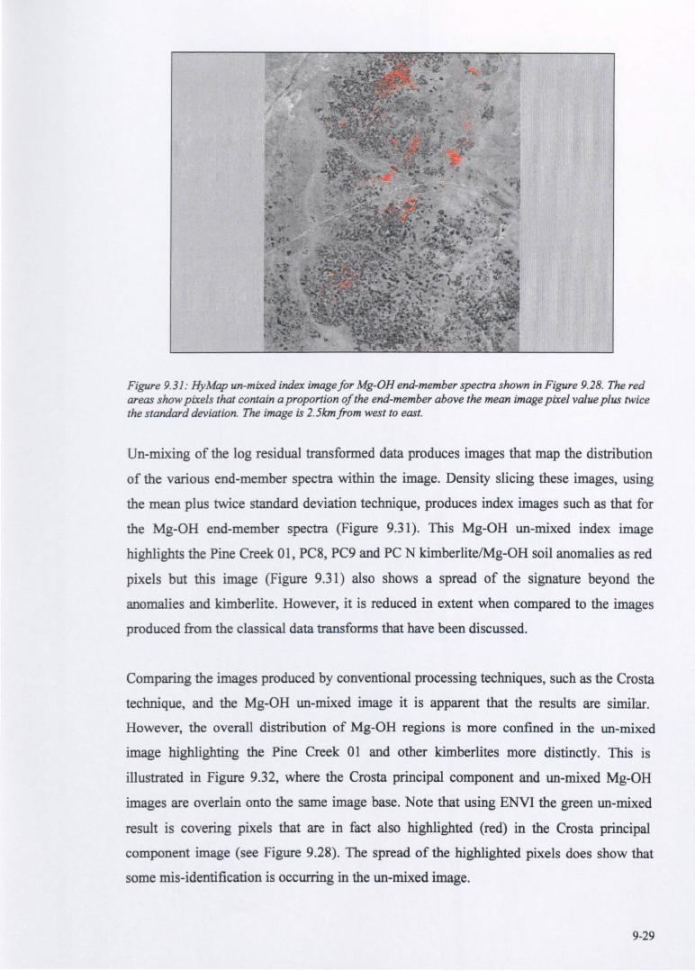
Figure 9.31: HyMap un-mixed index imagefor Mg-OH end-member spectra shown in Figure 9.28. The red areas show pixels that contain a proportion of the end-member above the mean image pixel value plus twice the standard deviation. The image is 2.5kmfrom west to east.

Un-mixing of the log residual transformed data produces images that map the distribution

of the various end-member spectra within the image. Density slicing these images, using

the mean plus twice standard deviation technique, produces index images such as that for

the Mg-OH end-member spectra (Figure 9.31). This Mg-OH un-mixed index image

highlights the Pine Creek 01, PC8, PC9 and PC N kimberlite/Mg-OH soil anomalies as red

pixels but this image (Figure 9.31) also shows a spread of the signature beyond the

anomalies and kimberlite. However, it is reduced in extent when compared to the images

produced from the classical data transforms that have been discussed.

Comparing the images produced by conventional processing techniques, such as the Crosta

technique, and the Mg-OH un-mixed image it is apparent that the results are similar.

However, the overall distribution of Mg-OH regions is more confined in the un-mixed

image highlighting the Pine Creek 01 and other kimberlites more distinctly. This is

illustrated in Figure 9.32, where the Crosta principal component and un-mixed Mg-OH

images are overlain onto the same image base. Note that using ENVI the green un-mixed

result is covering pixels that are in fact also highlighted (red) in the Crosta principal

component image (see Figure 9.28). The spread of the highlighted pixels does show that

some mis-identification is occurring in the un-mixed image.

9-29

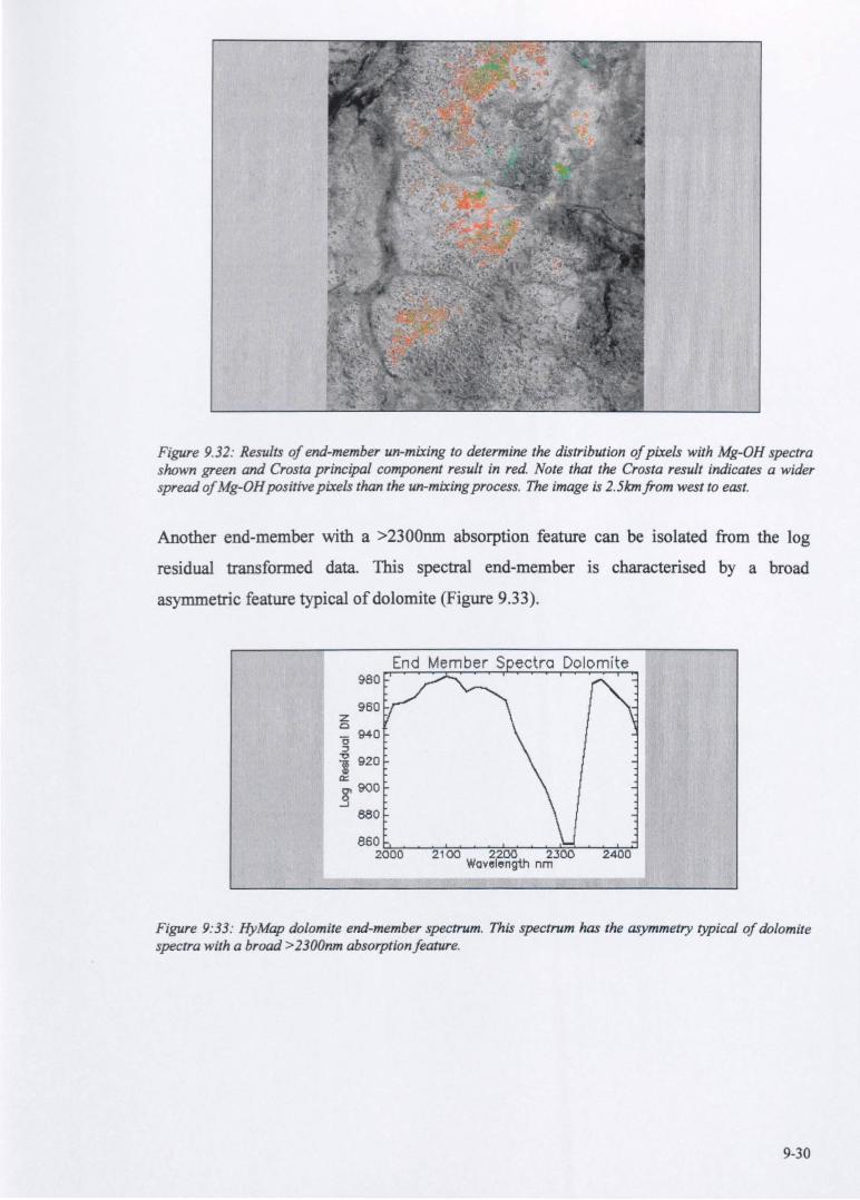
Figure 9.32: Results of end-member un-mixing to determine the distribution of pixels with Mg-OH spectra shown green and Crosta principal component result in red. Note that the Crosta result indicates a wider spread ofMg-OHpositivepixels than the un-mixing process. The image is 2.5kmfrom west to east.

Another end-member with a >2300nm absorption feature can be isolated from the log

residual transformed data. This spectral end-member is characterised by a broad

asymmetric feature typical of dolomite (Figure 9.33).

z o

980

960

-0 940 ::;)

1 920 a:: &' 900 ~

680

Figure 9:33: HyMap dolomite end-member spectrum. This spectrum has the asymmetry typical of dolomite spectra with a broad> 2300nm absorption feature.

9-30

1200

z 1180 0

"0 1160 :::>

" '0 1140 I) ~

g' 1120 ..:J

1100

Figure 9:34: RyMap AI-OR end-member spectrum.

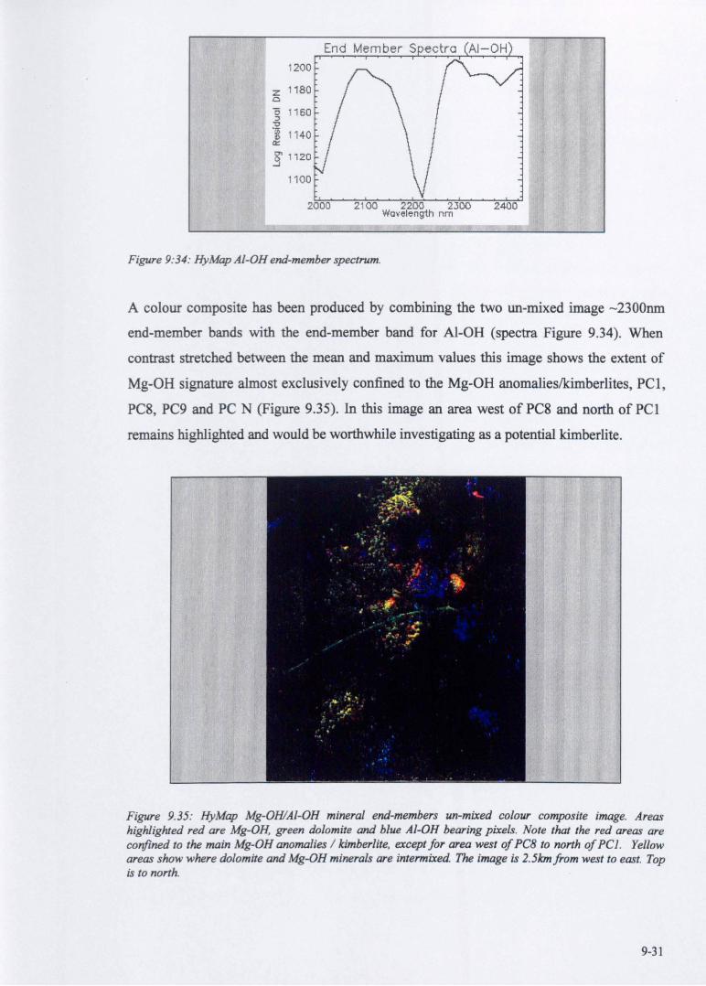
A colour composite has been produced by combining the two un-mixed image - 2300nm

end-member bands with the end-member band for Al-OH (spectra Figure 9.34). When

contrast stretched between the mean and maximum values this image shows the extent of

Mg-OH signature almost exclusively confined to the Mg-OH anomalieslkimberlites, PCI,

PC8, PC9 and PC N (Figure 9.35). In this image an area west of PC8 and north of PCI

remains highlighted and would be worthwhile investigating as a potential kimberlite.

Figure 9.35: RyMap Mg-OHIA1-OH mineral end-members un-mixed colour composite image. Areas highlighted red are Mg-OH. green dolomite and blue AI-OR bearing pixels. Note that the red areas are confined to the main Mg-OH anomalies / kimberlite. except for area west of PCB to north of PCl. Yellow areas show where dolomite and Mg-OH minerals are intermixed. The image is 2.5kmfrom west to east. Top is to north.

9-31

Comments

Of the conventional processing techniques investigated, the Crosta and anomaly prediction

technique index images provide the most interpretable results for discriminating the Mg­

OH regions of interest. These techniques are simple to apply using the ENVI software,

though the Crosta technique does require several iterations to determine the best

combination oftbree bands to input with the band of interest (2306nm).

The end-member un-mixing technique is interactive and time consuming, though this is

being addressed with improved software that should automate the end-member spectra

selection. The need for such automated processing will increase when satellite systems

such as ARIES produce vast amounts of data routinely (Huntington, 1997 pers. comm.).

This technique provides specific and consistent results with the advantage of selecting the

end-member of interest based on spectra that show only the Mg-OH characteristics.

This study shows that the Crosta principal component, Anomaly Residual Prediction and

end member un-mixing index techniques produce images that separate the dry vegetation

from Mg-OH spectral signatures. This is not achieved using the other conventional

processing techniques such as the Mg Score Band ratio and negative colour compo siting of

Log Residual transformed bands.

The combined end-member colour composite image separates the dolomite from Mg-OH

mineral regions. This separation better highlights the Pine Creek 01 kimberlite and

identifies other anomalies including PC8, PC9 and PC N which heavy mineral indicator

grain studies indicate are probable kimberlites (Shee. 1998 pers. comm.).

Discussion

The 1998 and previous field studies in the Pine Creek area confirm that saponite is

associated with the Pine Creek 01 kimberlite and other regions defined from the Mg-OH

end-member un-mixed image. These field studies have also confirmed the presence of

saponite in soils associated with the calcareous Callana formation rocks. The intermixing

of the dolomite and Mg-OH spectral end-members (yellow areas from red Mg-OH and

green dolomite) seen in the un-mixing colour composite image (Figure 9.35) supports the

observed association between saponite and calcareous sediments.

9-32

Graham (1967) postulates that weathering of dolomite with kaolinite present can produce

saponite; this reaction is enhanced by elevated temperatures and hydration (Post, 1984 and

Fulignati et al., 1997) associated with hydrothermal activity. Cowley and Priess (1997)

have stated that the Callana formation is an inlier of carbonate rich rocks. My field

observations suggest that the Callana formation can be classed as a dolomitic calc-arenite,

as these rocks contain a high proportion of quartz grains. Therefore, the intrusive event

associated with the emplacement of the kimberlite may have catalysed the formation of

saponite from the Callana formation sediments. This would have extended the area of

saponite beyond the limits of the kimberlite in this instance. Further studies into the

genesis of saponite in the soils would be worthwhile.

9.6 CONCLUSIONS FROM PINE CREEK SPECTRAL STUDIES

This investigation has shown that spectral studies in this region can locate kimberlites from

their Mg-OH spectral signature. It also reveals useful information on the mineralogy of the

regolith and soils in this area.

The study shows that HyMap scanner data, when appropriately processed (most reliably by

end-member un-mixing), can locate the areas of saponite associated with the kimberlites.

The static test with the GEOSCAN MkII scanner shows that data acquired from this

scanner have the potential to locate the saponite spectral signature associated with the Pine

Creek 01 kimberlite. Whether such data could be processed using Log Residual transforms

and end-member un-mixing to discriminate the 2306nm spectral signature (saponite) as

was achieved with the HyMap data, is not proven by this study.

The occurrence of saponite in this area, and its apparent association with both kimberlite

and Callana formation dolomitic rocks, requires further study. Unless there is a much

wider occurrence of kimberlite within the Callana formation, perhaps as widespread veins,

then the spread of saponite indicated by this study may be due to either:

• Weathering of the dolomitic rocks of the Callana formation which is producing the saponite, in which case the identification of saponite from remotely sensed data may result in misleading results when seeking kimberlites and other ultramafic rocks in dolomitic areas; or

• The thermal event associated with the kimberlite emplacement also produced saponite from the calc-arenites, which would be a rarer occurrence than if the saponite were produced by the weathering of dolomites alone.

9-33

Studies into the formation temperature of the saponite in this area would be required to

determine which of these possible explanations is correct. This might be achieved by using

oxygen isotope studies. In another area studied by the author, this technique confirmed that

a totally kaolinised kimberlite was the result of weathering, not hydrothermal alteration as

had been suspected (Pontual, 1995).

9-34

CHAPTER 10

10 TEST SITE STUDY - JUBILEE, KURNALPI AREA, WESTERN AUSTRALIA

10.1 INTRODUCTION

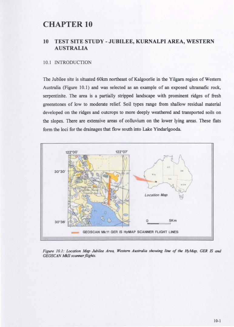
The Jubilee site is situated 60km northeast of Kalgoorlie in the Yilgarn region of West em

Australia (Figure 10.1) and was selected as an example of an exposed ultramafic rock,

serpentinite. The area is a partially stripped landscape with prominent ridges of fresh

greenstones of low to moderate relief Soil types range from shallow residual material

developed on the ridges and outcrops to more deeply weathered and transported soils on

the slopes. There are extensive areas of colluvium on the lower lying areas. These flats

form the loci for the drainages that flow south into Lake Yindarlgooda.

122"00· 122·0T

Lo~Uon tip

o SJ<m

GEOSCAN 11 GER IS HyMAP SCA ER FLlGIiT LINES

. , ..

Figure 10.1: Location Map Jubilee Area. Western Australia shOWing line of the HyMap, GER IS and GEOSCAN MklJ scanner flights.

10-1

The intrusive body investigated in this study is nearly rectangular and it is orientated

northwest southeast. This intrusive has a surface area of 150 hectares and intrudes into the

clastic sediments of the Mulgabbie formation. The petrographic report on this rock

(McMaster and Marx, 1984) states that it is a serpentinised peridotiteldunite. The geology

map of the area (Williams, 1973) identifies this intrusive as belonging to the Kalpini

formation ultramafic sequence that is identified as the youngest of the Archaean rocks in

the area. The margins of the body, particularly on the northern and southern sides, are

probably fault controlled. These shear zones have been investigated for gold and nickel

mineralisation and trenches have been dug across them. On the western side of the

intrusive, a northeast to southwest trending fault offsets it dextrally. Where this fault

extends northwards from the intrusive, trenches have been dug across it by mineral

exploration companies in previous years. This fault and the trenched area are clearly seen

in several of the HyMap processed images (Figure 10.25 to 10.27}

To the west, the margin of the intrusive is obscured by sand plain and lateritic duricrust

and in the east by colluvium. On the south and north, the contact with the clastic rocks is

exposed. A typica1lateritic weathering profile is developed on the clastic sediments to the

south of the intrusive. Two kilometres north of the intrusive, there is an outcrop of east­

west trending greenstones of the Mulgabbie formation. These rocks are described as

greenschist fitcies, basic to intermediate intrusives in the legend of the geology map

(Williams, 1973).

As Figure 3.1 shows, the area is sparsely vegetated with exposed soil and outcrop

comprising up to 70 percent of the region. There is no significant lichen development in

this area. However, on the southeastern side of the ultramafic, there are dense areas of

spinifex.

10-2

10.2 FIELD STUDIES

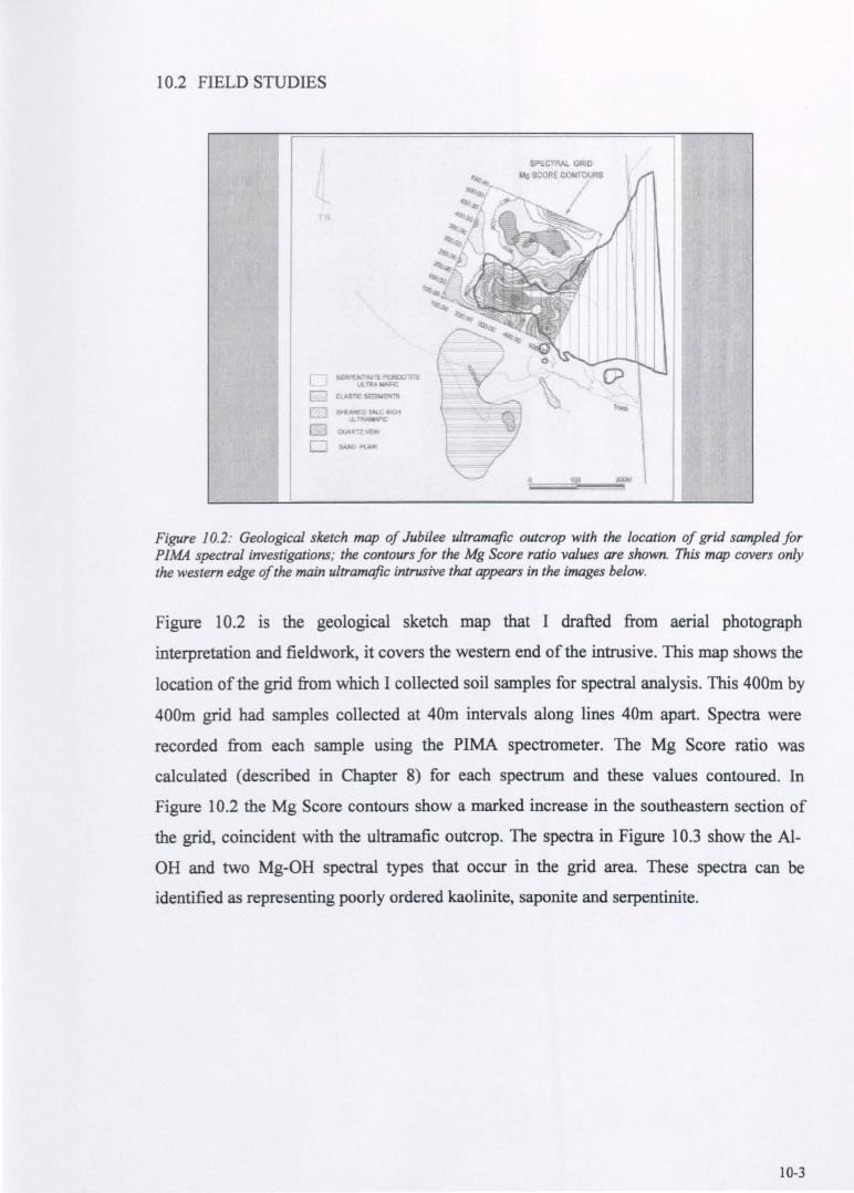
Figure 10.2: Geological sketch map of Jubilee ultramafic outcrop with the location of grid sampled for PIMA spectral investigations; the contours for the Mg Score ratio values are shown. This map covers only the western edge of the main ultramafic intrusive that appears in the images below.

Figure 10.2 is the geological sketch map that I drafted from aerial photograph

interpretation and fieldwork, it covers the western end of the intrusive. lbis map shows the

location of the grid from which I collected soil samples for spectral analysis. lbis 400m by

400m grid had samples collected at 40m intervals along lines 40m apart. Spectra were

recorded from each sample using the PIMA spectrometer. The Mg Score ratio was

calculated (described in Chapter 8) for each spectrum and these values contoured. In

Figure 10.2 the Mg Score contours show a marked increase in the southeastern section of

the grid, coincident with the ultramafic outcrop. The spectra in Figure 10.3 show the AJ­

OR and two Mg-OR spectral types that occur in the grid area. These spectra can be

identified as representing poorly ordered kaolinite, saponite and serpentinite.

10-3

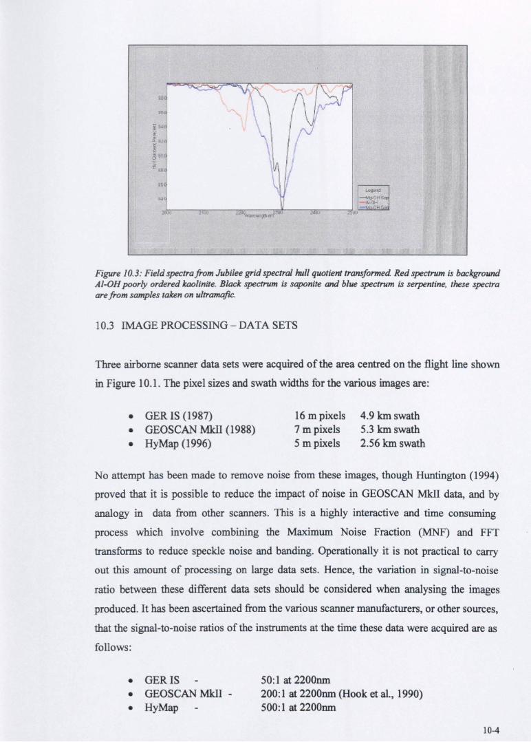
Figure 10.3: Field spectrafrom Jubilee grid spectral hull quotient transformed Red spectrum is background AI-OB poorly ordered kaolinite. Black spectrum is saponite and blue spectrum is serpentine, these spectra are from samples taken on ultramafic.

10.3 IMAGE PROCESSING - DATA SETS

Three airborne scanner data sets were acquired of the area centred on the flight line shown

in Figure 10.1. The pixel sizes and swath widths for the various images are:

• GER IS (1987) • GEOSCAN MkII (1988) • HyMap (1996)

16 m pixels 7 mpixels 5 mpixels

4.9 kmswath 5.3 kmswath 2.56 km swath

No attempt has been made to remove noise from these images, though Huntington (1994)

proved that it is possible to reduce the impact of noise in GEOSCAN MklI data, and by

analogy in data from other scanners. 1bis is a highly interactive and time consuming

process which involve combining the Maximum Noise Fraction (MNF) and FFT

transforms to reduce speckle noise and banding. Operationally it is not practical to carry

out this amount of processing on large data sets. Hence, the variation in signal-to-noise

ratio between these different data sets should be considered when analysing the images

produced. It has been ascertained from the various scanner manufacturers, or other sources,

that the signal-to-noise ratios of the instruments at the time these data were acquired are as

follows:

• GERIS • GEOSCAN MkII -• HyMap

50: 1 at 2200nm 200:1 at 2200nm (Hook et al., 1990) 500: 1 at 2200nm

10-4

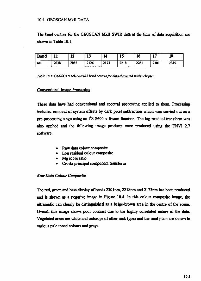
10.4 GEOSCAN MIdI DATA

The band centres for the GEOSCAN MIdI SWIR data at the time of data acquisition are

shown in Table 10.1.

BaDd 11 12 13 14 IS 16 17 18 run 2038 2085 2126 2173 2218 2261 2301 2345

Table 10.1: GEOSC4N MkI1 SWIRl band centres for data disctused in this chapter.

Conventional Image Processing

These data have had conventional and spectral processing applied to them. Processing

included removal of system offsets by dark pixel subtraction which was carried out as a

pre-processing stage using an I2S S600 software function. The log residual transform was

also applied and the following image products were produced using the ENVI 2.7

software:

• Raw data colour composite • Log residual colour composite • Mg score ratio • Crasta principal component transform

Raw Data ColoIII' Composite

The red, green and blue display of bands 2301nm, 2218nm and 2173nm has been produced

and is shown as a negative image in Figure 10.4. In this colour composite image, the

ultramafic can clearly be distinguished as a beige-brown area in the centre of the scene.

Overall this image shows poor contrast due to the highly correlated nature of the data.

Vegetated areas are white and outcrops of other rock types and the sand plain are shown in

various pale toned colours and greys.

10-5

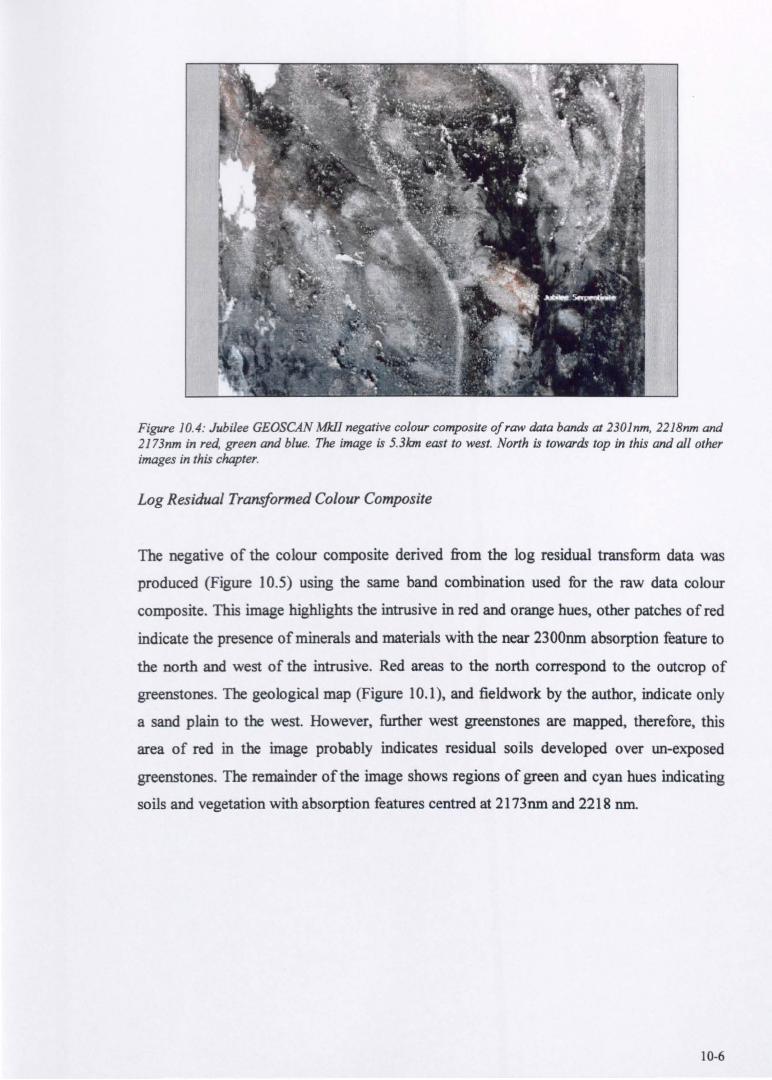
Figure 10.4: Jubilee GEOSCAN MkJ] negative colour composite of raw data bands at 2301nm, 2218nm and 2173nm in red, green and blue. The image is 5.3km east to west. North is towards top in this and all other images in this chapter.

Log Residual Transformed Colour Composite

The negative of the colour composite derived from the log residual transform data was

produced (Figure 10.5) using the same band combination used for the raw data colour

composite. This image highlights the intrusive in red and orange hues, other patches of red

indicate the presence of minerals and materials with the near 2300nm absorption feature to

the north and west of the intrusive. Red areas to the north correspond to the outcrop of

greenstones. The geological map (Figure 10.1), and fieldwork by the author, indicate only

a sand plain to the west. However, further west greenstones are mapped, therefore, this

area of red in the image probably indicates residual soils developed over un~exposed

greenstones. The remainder of the image shows regions of green and cyan hues indicating

soils and vegetation with absorption features centred at 2173nm and 2218 nm.

10-6

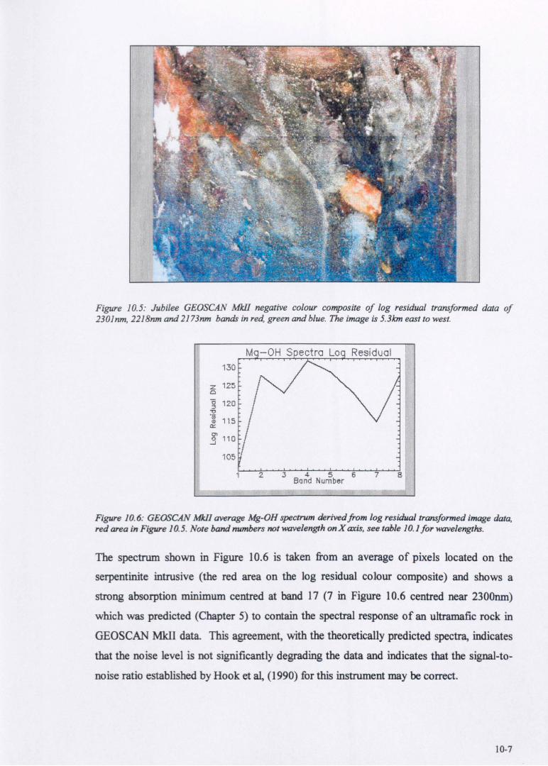
Figure 10.5: Jubilee GEOSCAN MkJJ negative colour composite of log residual transformed data of 2301nm, 2218nm and 2173nm bands in red, green and blue. The image is 5.3/cm east to west.

130

z 125 0

"0 120 j

ii 115 III

a::

.3 110

105

2 3 4 5 6 Band Number

7 8

Figure 10.6: GEOSCAN MJcJJ average Mg-OH spectrum derived from log residual transformed image data, red area in Figure 10.5. Note band numbers not wavelength on X axis, see table 10.1 for wavelengths.

The spectrum shown in Figure 10.6 is taken from an average of pixels located on the

serpentinite intrusive (the red area on the log residual colour composite) and shows a

strong absorption minimum centred at band 17 (7 in Figure 10.6 centred near 2300nm)

which was predicted (Chapter 5) to contain the spectral response of an ultramafic rock in

GEOSCAN MIdI data. This agreement, with the theoretically predicted spectra, indicates

that the noise level is not significantly degrading the data and indicates that the signal-to­

noise ratio established by Hook et at, (1990) for this instrument may be correct.

10-7

150

z Cl

140 1; J

"0 '(jj <ll

130 a::: (!I

.3 120

2 3 4 5 Bond Number

6 7 B

Figure 10.7: is a spectrum obtainedfrom an area of outcrop of clastic sediments situated to the south of the ultramafic outcrop; green on the log residual transform colour composite. This spectrum is that expected for

AI-OR clay, probably kaolinite and/or illite. Note band numbers (1-8=11-18) not wavelength on X axis, see Table 10.1 for wavelengths.

The green-cyan areas shown in Figure 10.5 show the distribution of AI-OH bearing

materials of which the spectrum shown in Figure 10.7 is typical, The near 2200nm

absorption feature, typical of AI-OH clays such as illite and kaolinite, occurring in band 15

(5 in Figure 10.7).

Mg Score Ratio

In this case, the Mg Score was derived by dividing band 2301nm (17) by 2218nm (15),

using the log residual transform data. The image produced (Figure 10.8) shows the Mg-OH

containing pixels in darker tones which are highlighted red in the index presentation. The

red pixels in this image highlight the serpentinised intrusive and also areas to the north and

northwest which, as mentioned above, are considered to be areas of thin residual soil

developed over greenstones.

10-8

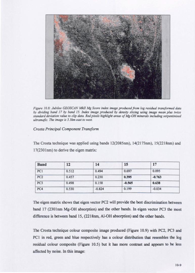
Figure 10.8: Jubilee GEOSCAN MIdI Mg Score index image produced from log residual transformed data by dividing band 17 by band 15. Index image produced by density slicing using image mean plus twice standard deviation value to clip data. Red pixels highlight areas of Mg-OR minerals including serpentinised ultramafic. The image is 5.3km east to west.

Crosta Principal Component Transform

The Crosta technique was applied using bands 12(2085nm), 14(2173nm), 15(2218nm) and

17(230Inm) to derive the eigen matrix:

Band 12 14 15 17

PC1 0.512 0.494 0.697 0.095

PC2 0.457 0.230 0.395 -0.763

PC3 0.498 0.158 -0.565 0.638

PC4 0.530 -0.824 0.l99 -0.034

The eigen matrix shows that eigen vector PC2 will provide the best discrimination between

band 17 (2301nm Mg-OH absorption) and the other bands. In eigen vector PC3 the most

difference is between band 15, (2218nm, Al-OH absorption) and the other bands.

The Crosta technique colour composite image produced (Figure 10.9) with PC2, PC3 and

PCI in red, green and blue respectively has a colour distribution that resembles the log

residual colour composite (Figure 10.5) but it has more contrast and appears to be less

affected by noise. In this image:

10-9

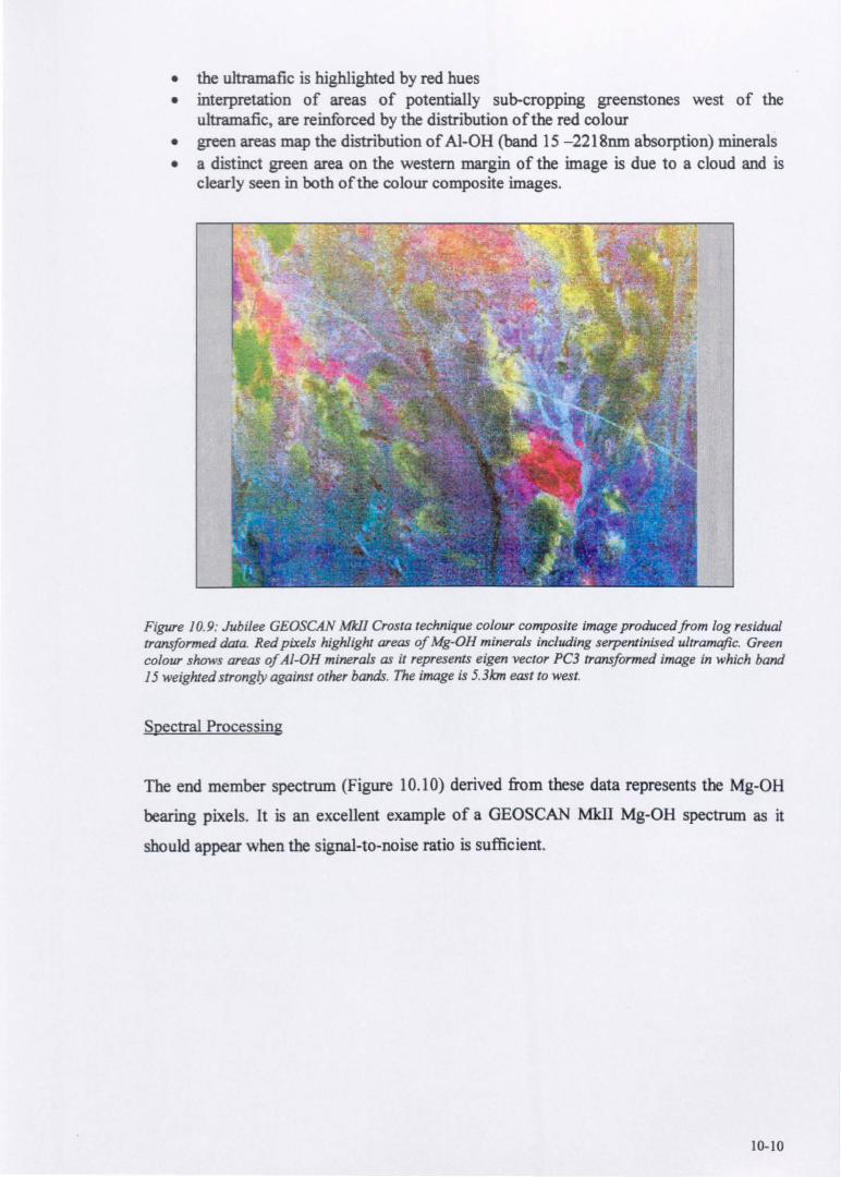
• the ultramafic is highlighted by red hues • interpretation of areas of potentially sub-cropping greenstones west of the

ultramafic, are reinforced by the distribution of the red colour • green areas map the distribution of Al-OH (band 15 -2218nm absorption) minerals • a distinct green area on the western margin of the image is due to a cloud and is

clearly seen in both of the colour composite images.

Figure 10.9: Jubilee GEOSCAN MkII Crosta technique colour composite image producedfrom log residual transformed data. Red pixels highlight areas of Mg-OR minerals including serpentinised ultramafic. Green colour shows areas of AI-OR minerals as it represents eigen vector PC3 transformed image in which band 15 weighted strongly against other bands. The image is 5.3km east to west.

Spectral Processing

The end member spectrum (Figure 10.10) derived from these data represents the Mg-OH

bearing pixels. It is an excellent example of a GEOSCAN MklI Mg-OH spectrum as it

should appear when the signal-to-noise ratio is sufficient.

10-10

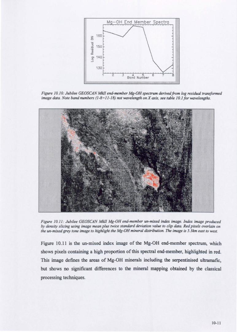
z 160 c

"0 ::l 150

1 a:: 8' 140

...:.J

130

2 .3 4 5 6 Bend Number

8

Figure 10.10: Jubilee GEOSCAN Mkll end-member Mg-OH spectrum derivedfrom log residual transformed image data. Note band numbers (J -8= 11 -1 8) not -wavelength on X axis, see table 10.1 for wavelengths.

Figure 10.1 J: Jubilee GEOSCAN Mk11 Mg-OH end-member un-mixed index image. Index image produced by density sliCing using image mean plus twice standard deviation value to clip data. Red pixels overlain on the un-mixed grey tone image to highlight the Mg-OH mineral distribution. The image is 5.3km east to west.

Figure 10.11 is the un-mixed index image of the Mg-OH end-member spectrum, which

shows pixels containing a high proportion of this spectral end-member, highlighted in red.

This image defines the areas of Mg-OH minerals including the serpentinised ultramafic,

but shows no significant differences to the mineral mapping obtained by the classical

processing techniques.

10-11

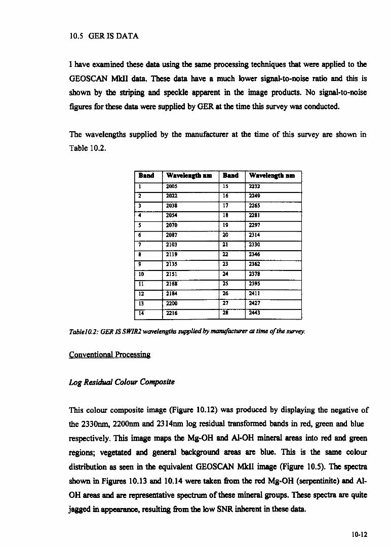
10.5 GERIS DATA

I have examined these data using the same processing techniques that were applied to the

GEOSCAN MkII data. These data have a much lower signal-to-noise ratio and this is

shown by the striping and speckle apparent in the image products. No signal-to-noise

figures for these data were supplied by GER at the time this survey was conducted.

The wavelengths supplied by the manufacturer at the time of this survey are shown in

Table 10.2.

Bud Wavelellatb IUD Bud Waveleqtb IUD

1 200S IS 2232

2 2022 16 2249

3 2038 17 2265

4 2054 18 2281

5 2070 19 2297

6 2087 20 2314

7 2103 21 2330

8 2119 22 2346

9 2135 23 2362

10 2151 24 2378

11 2168 25 2395

12 2184 26 2411

13 2200 27 2427

14 2216 28 2443

TablelO.2: GER IS SWIRl wavelengths supplied by manu/actul'e1' at time a/the survey.

Conventional Processing

Log Residual CoioUl' Composite

This colour composite image (Figure 10.12) was produced by displaying the negative of

the 2330nm, 2200nm and 2314nm log residual transformed bands in red, green and blue

respectively. This image maps the Mg-OH and Al-OH mineral areas into red and green

regions; vegetated and general background areas are blue. This is the same colour

distribution as seen in the equivalent GEOSCAN MkII image (Figure 10.S). The spectra

shown in Figures 10.13 and 10.14 were taken from the red Mg-OH (serpentinite) and AI­

OH areas and are representative spectrum of these mineral groups. These spectra are quite

jagged in appearance, resulting from the low SNR inherent in these data.

10-12

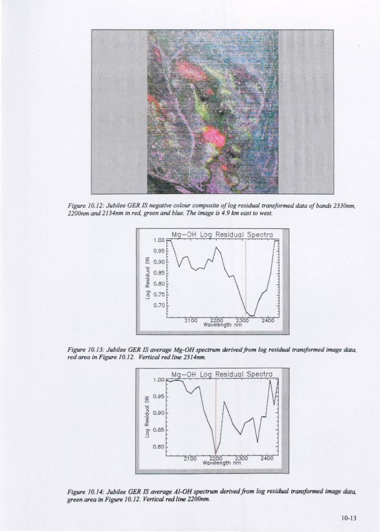
Figure 10.12: Jubilee GER IS negative colour composite of log residual transformed data of bands 2330nm, 2200nm and 2134nm in red, green and blue. The image is 4.9 /em east to west.

1.00

0 ,95

z 0.90 Cl

C 0.85 :J

" 'r;; Q) 0,80 ~

.3 0,75

0 ,70

Figure 10.13: Jubilee GER IS average Mg-OR spectrum derived from log residual transformed image data, red area in Figure 10.12. Vertical red line 2314nm.

z Q.95 Cl

C :J 0.90 ~ Q)

~

8' 0,85 ..:.J

0.80

21 Q() 2200 2300 2400 Wavelength nm

Figure 10.14: Jubilee GER IS average AI-OR spectrum derived from log residual transformed image data, green area in Figure 10.12. Vertical red line 2200nm.

10-13

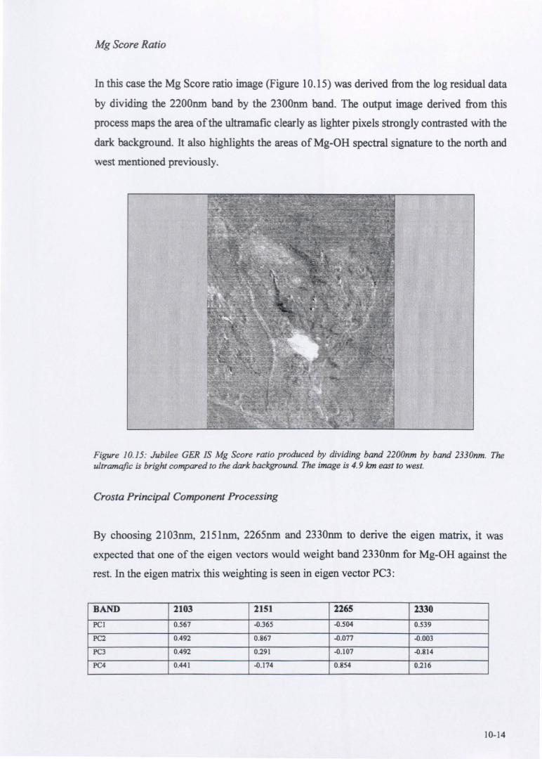
Mg Score Ratio

In this case the Mg Score ratio image (Figure 10.15) was derived from the log residual data

by dividing the 2200nm band by the 2300nm band. The output image derived from this

process maps the area of the ultramafic clearly as lighter pixels strongly contrasted with the

dark background. It also highlights the areas of Mg-OH spectral signature to the north and

west mentioned previously.

Figure 10.15: Jubilee GER IS Mg Score ratio produced by dividing band 2200nm by band 2330nm. The ultramafic is bright compared to the dark background. The image is 4.9 km east to west.

Crosta Principal Component Processing

By choosing 2103nm, 2151nm, 2265nm and 2330nm to derive the eigen matrix, it was

expected that one of the eigen vectors would weight band 2330nm for Mg-OH against the

rest. In the eigen matrix this weighting is seen in eigen vector PC3:

BAND 2103 21S1 1165 2330

PCI 0.567 -0.365 -0.504 0.539

PC2 0.492 0.867 -0.077 -0.003

PC3 0.492 0.291 -0.107 -0.814

PC4 0.441 -0.174 0.854 0.216

10-14

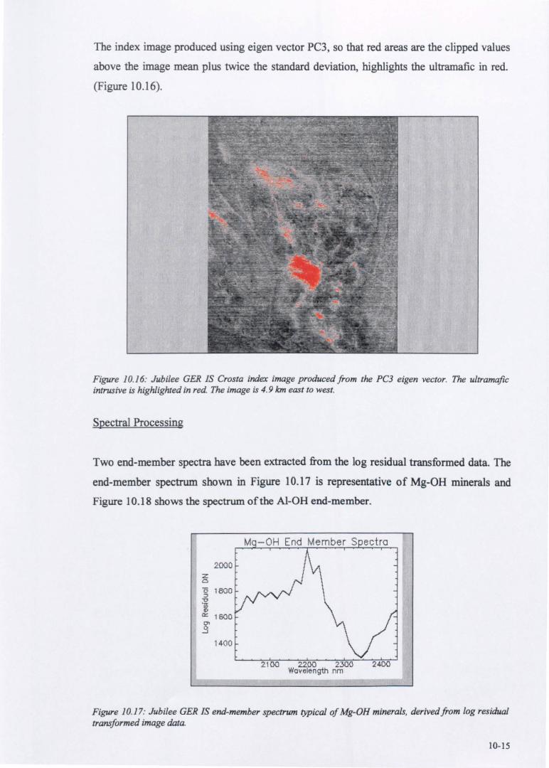
The index image produced using eigen vector PC3, so that red areas are the clipped values

above the image mean plus twice the standard deviation, highlights the ultramafic in red.

(Figure 10.16).

Figure 10.16: Jubilee GER IS Crosta index image produced from the PC3 eigen vector. The ultramafic intrusive is highlighted in red The image is 4.9 Ian east to west.

Spectral Processing

Two end-member spectra have been extracted from the log residual transformed data. The

end-member spectrum shown in Figure 10.17 is representative of Mg-OH minerals and

Figure 10.18 shows the spectrum of the Al-OH end-member.

z 0

(3 180 0 ::;, -c 'ih II> ~

0'1

.9 1400

Figure 10.17: Jubilee GER IS end-member spectrum typical of Mg-OH minerals, derived from log residual transformed image data.

10-15

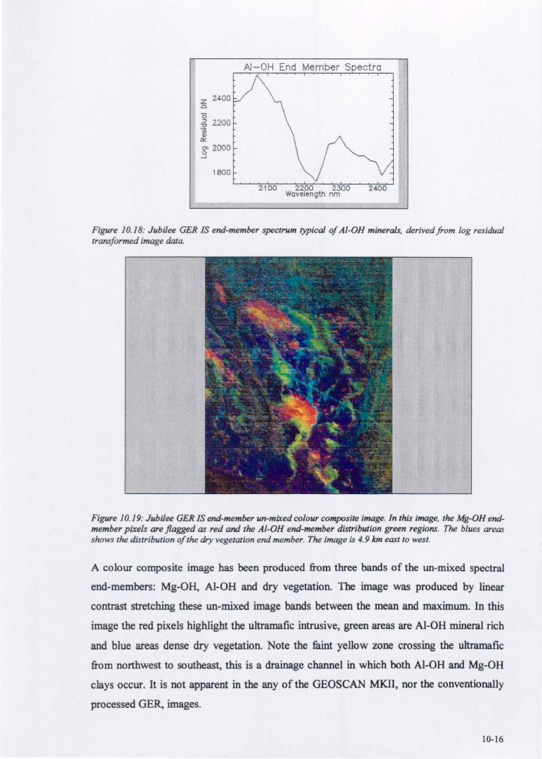
z 2400 o 15 -6 22()O ] a:: 8' 2000 ~

1800

2100 2200 2300 Wavelength nm

Figure 10.18: Jubilee GER IS end-member spectrum typical of AI-OB minerals, derived from log residual transformed image data.

Figure 10. 19: Jubilee GER IS end-member un-mixed colour composite image. In this image, the Mg-OB end­member pixels are flagged as red and the AI-OB end-member distribution green regions. The blues areas shows the distribution of the dry vegetation end member. The image is 4.9 Ion east to west.

A colour composite image has been produced from three bands of the un-mixed spectral

end-members: Mg-OH, Al-OH and dry vegetation. The image was produced by linear

contrast stretching these un-mixed image bands between the mean and maximum. In this

image the red pixels highlight the ultramafic intrusive, green areas are Al-OH mineral rich

and blue areas dense dry vegetation. Note the faint yellow zone crossing the ultramafic

from northwest to southeast, this is a drainage channel in which both Al-OH and Mg-OH

clays occur. It is not apparent in the any of the GEOSCAN MKlI, nor the conventionally

processed GE~ images.

10-16

10.6 HyMap DATA

These data have been processed with the same techniques applied to other scanner imagery

in this study. As the HyMap has a smaller pixel size than the other data sets its images only

represent a subsection of the area seen in the GEOSCAN MkII and GER IS images. The

effect of this reduced pixel size on the spatial resolution of the data is immediately

apparent; minor creeks and individual trees are clearly discernible in the HyMap images.

Such detail is not seen in the other scanner data sets.

Conventional Processing

Raw Data Colour Composite

The negative colour composite derived from the raw data is shown in Figure 10.20 and has

bands 2318nm, 2203nm and 2lSOnm displayed in red, green and blue respectively. This

image is similar in appearance to the GEOSCAN MKII colour composite (Figure 10.4) of

this area. In this HyMap colour composite the serpentinite is highlighted in red-purple hues

while the remainder of the image has pastel shades of grey, cyan and green. Vegetation,

trees and clumps of bushes are white in this image rendition. This image also indicates that

there are some dense patches of vegetation developed on the southeastern side of the

serpentinite. Field visits have shown that this is spinifex. The letters S, V and DG

annotated on the image indicate where spectra have been extracted from the log residual

transform of these data.

10-17

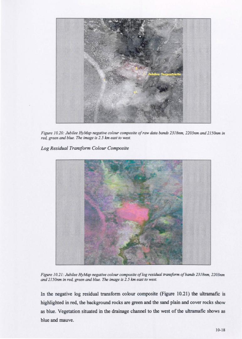
Figure 10.20: Jubilee HyMap negative colour composite of raw data bands 2318nm, 2203nm and 2150nm in red, green and blue. The image is 2.5 km east to west.

Log Residual Transform Colour Composite

Figure 10.21 : Jubilee HyMap negative colour composite of log residual transform of bands 2318nm, 2203nm and 21 50nm in red, green and blue. The image is 2.5 km east to west.

In the negative log residual transform colour composite (Figure 10.21) the ultramafic is

highlighted in red, the background rocks are green and the sand plain and cover rocks show

as blue. Vegetation situated in the drainage channel to the west of the ultramafic shows as

blue and mauve.

10-18

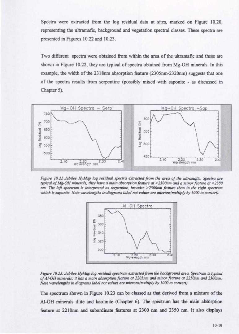
Spectra were extracted from the log residual data at sites, marked on Figure 10.20,

representing the ultramafic, background and vegetation spectral classes. These spectra are

presented in Figures 10.22 and 10.23.

Two different spectra were obtained from within the area of the ultramafic and these are

shown in Figure 10.22, they are typical of spectra obtained from Mg-OR minerals. In this

example, the width of the 2318nm absorption feature (2305nm-2320nm) suggests that one

of the spectra resuhs from serpentine (possibly mixed with saponite - as discussed in

Chapter 5).

750

z 700 Q

"0 650 :::l

~ Q! 600

a::

.3 550

500

Z Q

o

600

::l 550 ~ Q!

a::

.3 500

450~~~~ __ ~~~~~ ____ ~ 2.10 2 .20 2.30 2.41

Wavelength nm

Figure 10.22 Jubilee HyMap log residual spectra extracted from the area of the ultramafic. Spectra are typical of Mg-OH minerals. they have a main absotption feature at > 2300nm and a minor feature at >2380 nm. The left spectrum is intetpreted as serpentine, broader > 2300nm feature than in the right spectrum which is saponite. Note wavelengtru in diagrams label not values are microns(multiply by 1000 to convert).

z £:)

380

o 360 ::l

""0

li 340 a:: 0\ .3 320

300

Figure 10.23: Jubilee HyMap log residual spectrum extractedfrom the background area. Spectrum is typical of AI-OH minerals; it has a main absotptionfeature at 2203nm and minor feature at 2250nm and 2300nm. Note wavelengths in diagrams labe/not values are microns(multiply by 1000 to convert).

The spectrum shown in Figure 10.23 can be classed as that derived from a mixture of the

AI-OR minerals illite and kaolinite (Chapter 6). The spectrum bas the main absorption

feature at 2210nm and subordinate features at 2300 nm and 2350 nm. It also displays

10- 19

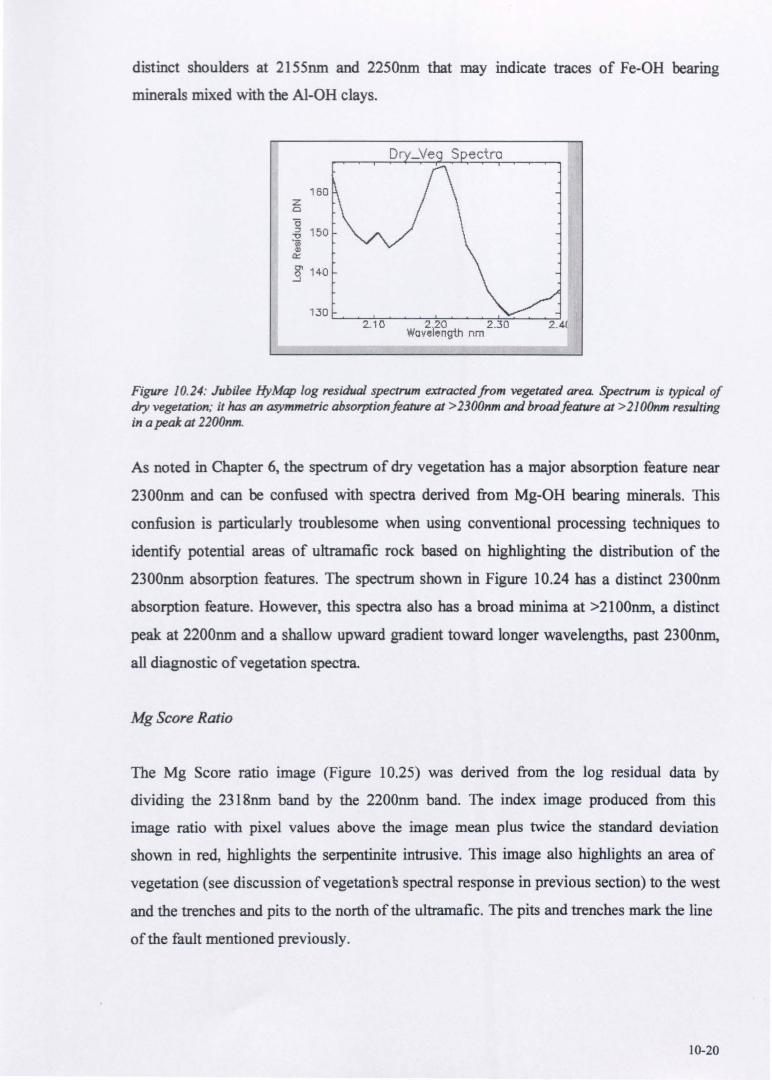
distinct shoulders at 2155nm and 2250nm that may indicate traces of Fe-OH bearing

minerals mixed with the Al-OH clays.

z o

"'0

160

~ 150 1 a:::

8' 140 ...;J

Figure 10.24: Jubilee HyMap log residual spectrum extracted from vegetated area. Spectrum is typical of dry vegetation; it has an asymmetric absorptionfeature at >2300nm and broadfoature at >210Onm resulting in apeak at 2200nm.

As noted in Chapter 6, the spectrum of dry vegetation has a major absorption feature near

2300nm and can be confused with spectra derived from Mg-OH bearing minerals. This

confusion is particularly troublesome when using conventional processing techniques to

identify potential areas of ultramafic rock based on highlighting the distribution of the

2300nm absorption features. The spectrum shown in Figure 10.24 has a distinct 2300nm

absorption feature. However, this spectra also has a broad minima at >2100nm, a distinct

peak at 2200nm and a shallow upward gradient toward longer wavelengths, past 2300nm,

all diagnostic of vegetation spectra.

Mg Score Ratio

The Mg Score ratio image (Figure 10.25) was derived from the log residual data by

dividing the 2318nm band by the 2200nm band. The index image produced from this

image ratio with pixel values above the image mean plus twice the standard deviation

shown in red, highlights the serpentinite intrusive. This image also highlights an area of

vegetation (see discussion of vegetations spectral response in previous section) to the west

and the trenches and pits to the north of the ultramafic. The pits and trenches mark the line

of the fault mentioned previously.

10-20

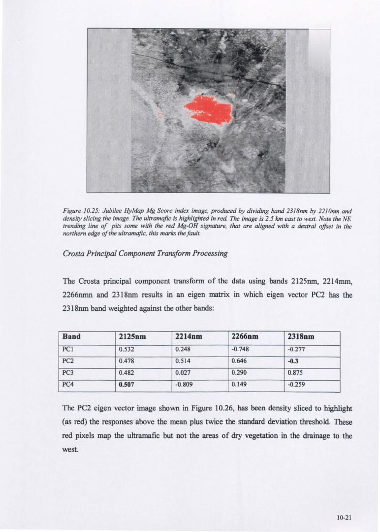
Figure 10.25: Jubilee HyMap Mg Score index image, produced by dividing band 2318nm by 2210nm and density slicing the image. The ultramafic is highlighted in red. The image is 2.5 Ian east to west. Note the NE trending line of pits some with the red Mg-OH signature, that are aligned with a dextral offset in the northern edge of the ultramafic, this marks the/ault.

Crosta Principal Component Transform Processing

The Crosta principal component transform of the data using bands 2125nm, 2214mm,

2266nmn and 2318nm results in an eigen matrix in which eigen vector PC2 has the

2318nm band weighted against the other bands:

Band 2125nm 2214nm 2266nm 2318nm

PCl 0.532 0.248 -0.748 -0.277

PC2 0.478 0.514 0.646 -0.3

PC3 0.482 0.027 0.290 0.875

PC4 0.507 -0.809 0.149 -0.259

The PC2 eigen vector image shown in Figure 10.26, has been density sliced to highlight

(as red) the responses above the mean plus twice the standard deviation threshold. These

red pixels map the ultramafic but not the areas of dry vegetation in the drainage to the

west.

10-21

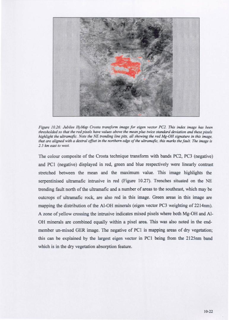
Figure 10.26: Jubilee HyMap Crosta transform image for eigen vector PC2. This index image has been thresholded so that the red pixels have values above the mean plus twice standard deviation and these pixels highlight the ultramafic. Note the NE trending line pits, all showing the red Mg-OH signature in this image, that are aligned with a dextral offiet in the northern edge of the ultramafic, this marks the fault. The image is 2.5 /em east to west.

The colour composite of the Crosta technique transform with bands PC2, PC3 (negative)

and PCI (negative) displayed in red, green and blue respectively were linearly contrast

stretched between the mean and the maximum value. This image highlights the

serpentinised ultramafic intrusive in red (Figure 10.27). Trenches situated on the NE

trending fault north of the ultramafic and a number of areas to the southeast, which may be

outcrops of ultramafic rock, are also red in this image. Green areas in this image are

mapping the distribution of the Al-OH minerals (eigen vector PC3 weighting of 2214nm).

A zone of yellow crossing the intrusive indicates mixed pixels where both Mg-OH and Al­

OH minerals are combined equally within a pixel area. This was also noted in the end­

member un-mixed GER image. The negative of PCI is mapping areas of dry vegetation;

this can be explained by the largest eigen vector in PCI being from the 2125nm band

which is in the dry vegetation absorption feature.

10-22

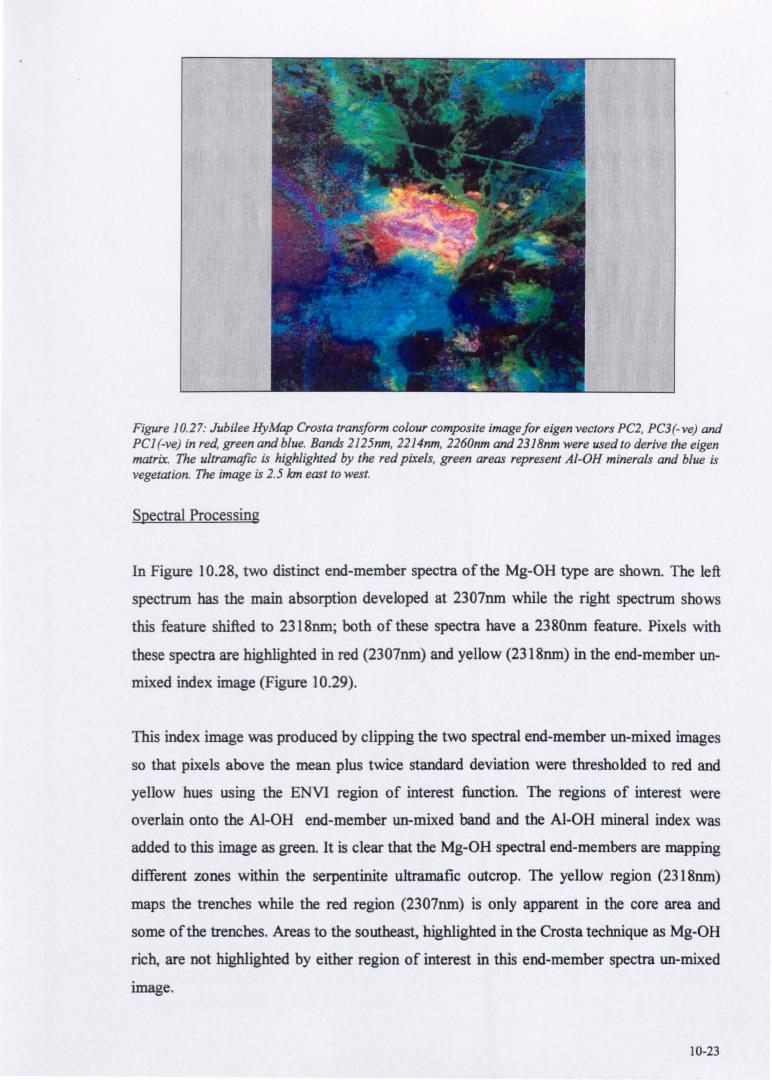
Figure 10.27: Jubilee HyMap Crosta transform colour composite imagefor eigen vectors PC2, PC3(-ve) and PC1 (-ve) in red, green and blue. Bands 2125nm, 2214nm, 2260nm and 2318nm were used to derive the eigen matrix. The ultramafic is highlighted by the red pixels, green areas represent AI-OH minerals and blue is vegetation. The image is 2.5 Ian east to west.

Spectral Processing

In Figure 10.28, two distinct end-member spectra of the Mg-OH type are shown. The left

spectrum has the main absorption developed at 2307nm while the right spectrum shows

this feature shifted to 2318nm; both of these spectra have a 2380nm feature. Pixels with

these spectra are highlighted in red (2307nm) and yellow (2318nm) in the end-member un­

mixed index image (Figure 10.29).

This index image was produced by clipping the two spectral end-member un-mixed images

so that pixels above the mean plus twice standard deviation were thresholded to red and

yellow hues using the ENVI region of interest function. The regions of interest were

overlain onto the Al-OH end-member un-mixed band and the Al-OH mineral index was

added to this image as green. It is clear that the Mg-OH spectral end-members are mapping

different zones within the serpentinite ultramafic outcrop. The yellow region (2318nm)

maps the trenches while the red region (2307nm) is only apparent in the core area and

some of the trenches. Areas to the southeast, highlighted in the Crosta technique as Mg-OH

rich, are not highlighted by either region of interest in this end-member spectra un-mixed

image.

10-23

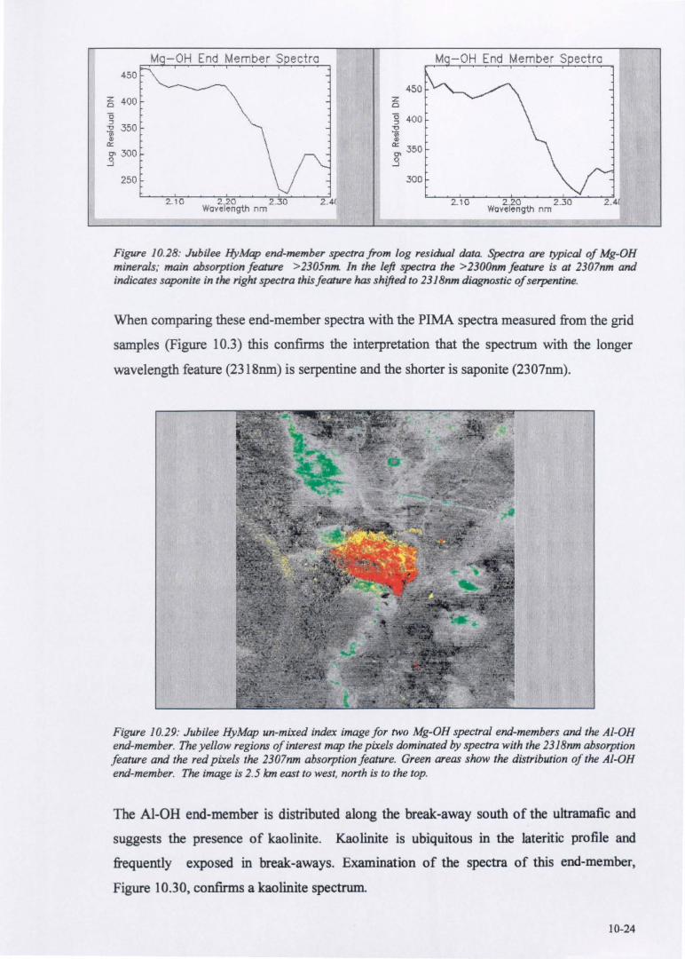
450

E 400

"0

~ 350 11 ~

0'1300 ..9

250

M -OH End Member S ectro

2-10

z Cl

450

g 400

1 ~ 350 0'1

..9 300

M -OH End Member S ect ro

2.10 220 2..30 wavelength nm

Figure 10.28: Jubilee HyMap end-member spectra from log residual data. Spectra are typical of Mg-OB minerals; main absorption feat/ire > 2305nm. In the left spectra the> 2300nm foature is at 2307nm and indicates saponite in the right spectra this feature has shifted to 2318nm diagnostic of serpentine.

When comparing these end-member spectra with the PIMA spectra measured from the grid

samples (Figure 10.3) this confirms the interpretation that the spectrum with the longer

wavelength feature (2318nm) is serpentine and the shorter is saponite (2307nm).

Figure 10.29: Jubilee HyMap un-mixed index image for two Mg-OH spectral end-members and the AI-DB end-member. The yellow regions of interest map the pixels dominated by spectra with the 2318nm absorption feature and the red pixels the 2307nm absorption feature. Green areas show the distribution of the AI-DB end-member. The image is 2.5 kin east to west, north is to the top.

The Al-OH end-member is distributed along the break-away south of the ultramafic and

suggests the presence of kaolinite. Kaolinite is ubiqujtous in the lateritic profile and

frequently exposed in break-aways. Examination of the spectra of this end-member,

Figure 10.30, confirms a kaolinhe spectrum.

10-24

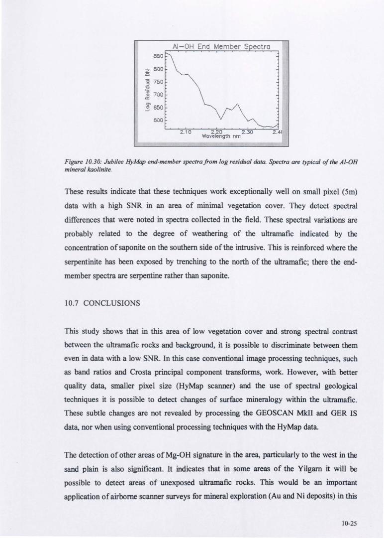
850

z 8GO a

"Ii 750 "U

.~ 700 £t:

.3 650

600

AI-OH End Member S ectro

2.. 10 2.20 2.30 2.4( Wavelength nm

Figure 10.30: Jubilee HyMap end-member spectrafrom log residual data. Spectra are typical of the AI-OB mineral kaolinite.

These resuhs indicate that these techniques work exceptionally well on small pixel (Sm)

data with a high SNR in an area of minimal vegetation cover. They detect spectral

differences that were noted in spectra collected in the field. These spectral variations are

probably related to the degree of weathering of the ultramafic indicated by the

concentration ofsaponite on the southern side of the intrusive. This is reinforced where the

serpentinite has been exposed by trenching to the north of the ultramafic; there the end­

member spectra are serpentine rather than saponite.

10.7 CONCLUSIONS

This study shows that in this area of low vegetation cover and strong spectral contrast

between the ultramafic rocks and background, it is possible to discriminate between them

even in data with a low SNR. In this case conventional image processing techniques, such

as band ratios and Crosta principal component transforms, work. However, with better

quality data, smaller pixel size (HyMap scanner) and the use of spectral geological

techniques it is possible to detect changes of surface mineralogy within the ultramafic.

These subtle changes are not revealed by processing the GEOSCAN MklI and GER IS

data, nor when using conventional processing techniques with the HyMap data.

The detection of other areas of Mg-OH signature in the area, particularly to the west in the

sand plain is also significant. It indicates that in some areas of the Yilgam it will be

possible to detect areas of unexposed ultramafic rocks. This would be an important

application of airborne scanner surveys for mineral exploration (Au and Ni deposits) in this

10-25

region. Such resuhs, if combined with the investigation of aeromagnetic data (Arvind,

1990) which can also indicate the occurrence of unexposed ultramafic rocks, could

improve targeting areas with potential for mineralisation. This study suggests that data of

the HyMap quality, ifprocessed spectrally, would certainly benefit such investigations.

10-26

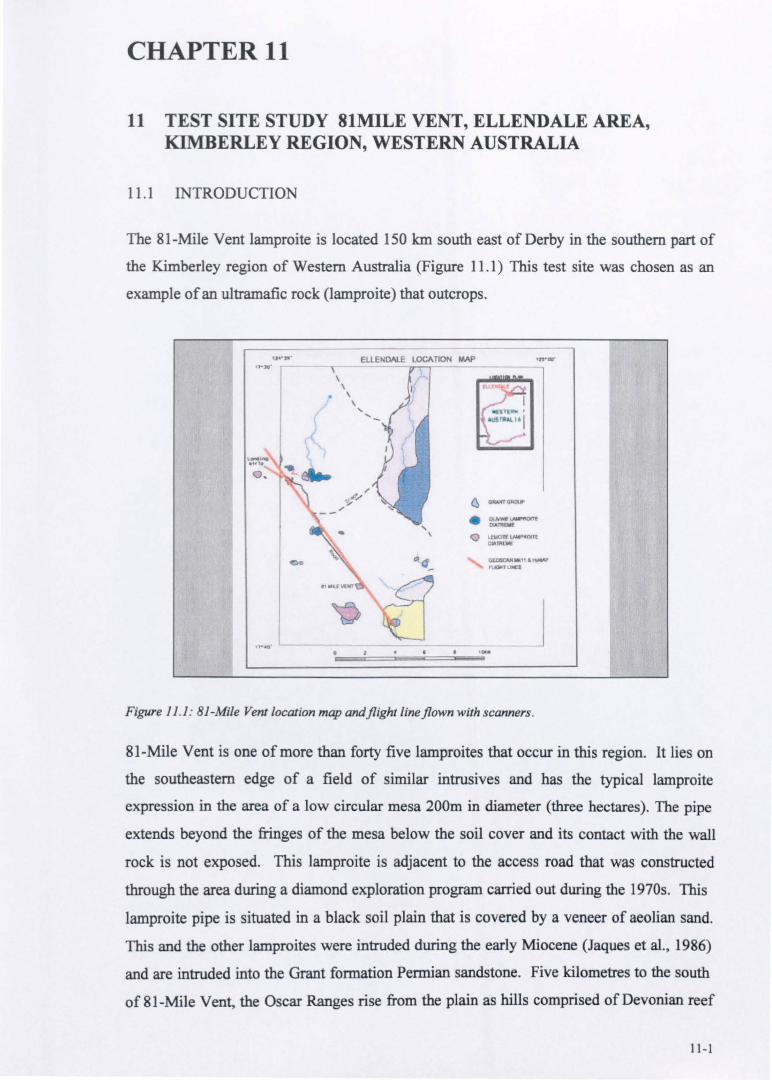
CHAPTER 11

11 TEST SITE STUDY 81MILE VENT, ELLENDALE AREA, KIMBERLEY REGION, WESTERN AUSTRALIA

11.1 INTRODUCTION

The 81-Mile Vent lamproite is located 150 km south east of Derby in the southern part of

the Kimberley region of Western Australia (Figure 11.1) This test site was chosen as an

example of an ultramafic rock (lamproite) that outcrops.

.,..,,' ElleNDAlE LOCAT1ON MAP 'H'.' H'.' ,

\

~ \

\ '- ....

" ... ~ ~ ....",. ......

" ,;

• ...,. -.. ... ,..... """'~ ""' ..

eo • '-'*Nt .. " I.WfMAII '.fl.1III€I

11· .. • --.....

Figure 11.1: B1-Mile Vent location map andflight line flown with scanners.

81-Mile Vent is one of more than forty five lamproites that occur in this region. It lies on

the southeastern edge of a field of similar intrusives and has the typical lamproite

expression in the area of a low circular mesa 200m in diameter (three hectares). The pipe

extends beyond the fringes of the mesa below the soil cover and its contact with the wall

rock is not exposed. This lamproite is adjacent to the access road that was constructed

through the area during a diamond exploration program carried out during the 1970s. This

lamproite pipe is situated in a black soil plain that is covered by a veneer of aeolian sand.

This and the other lamproites were intruded during the early Miocene (Jaques et aI., 1986)

and are intruded into the Grant formation Permian sandstone. Five kilometres to the south

of 81-Mile Vent, the Oscar Ranges rise from the plain as hills comprised of Devonian reef

11-1

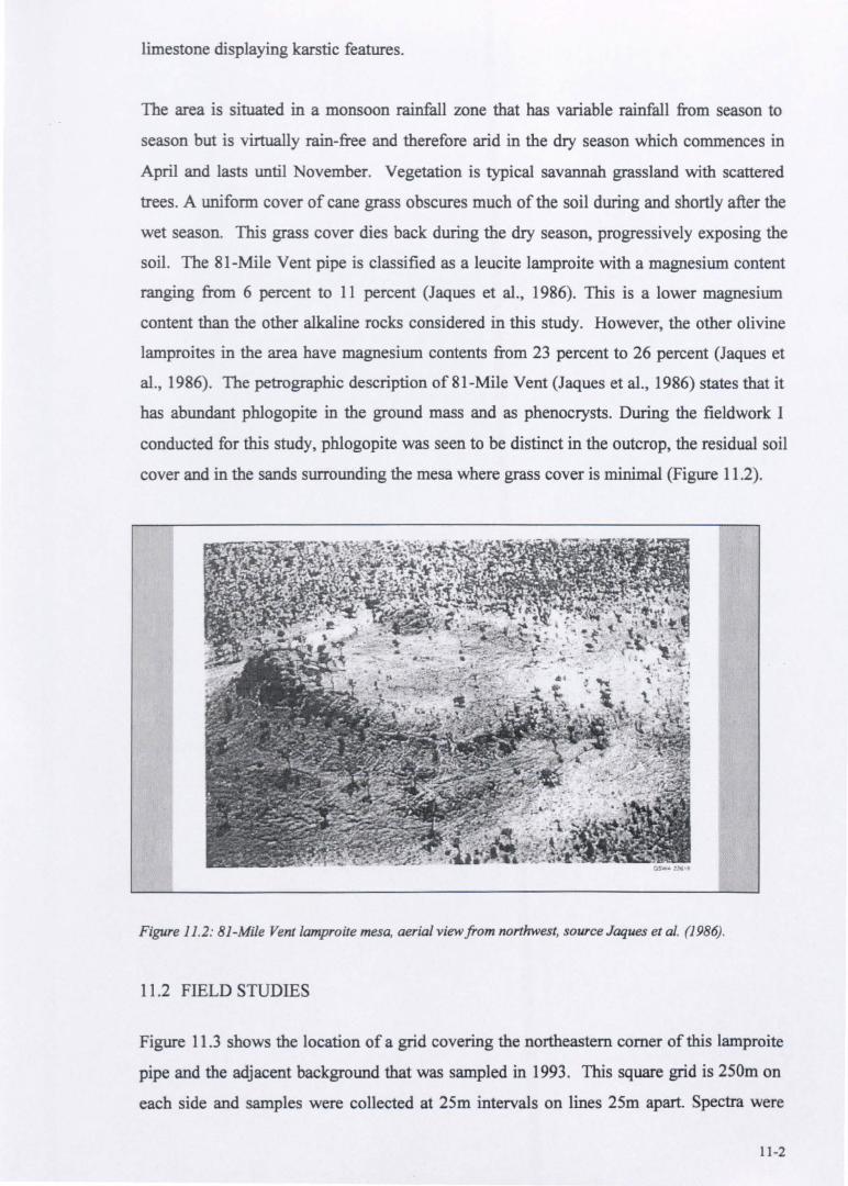
limestone displaying karstic features.

The area is situated in a monsoon rainfall zone that has variable rainfall from season to

season but is virtually rain-free and therefore arid in the dry season which commences in

April and lasts until November. Vegetation is typical savannah grassland with scattered

trees. A uniform cover of cane grass obscures much of the soil during and shortly after the

wet season. This grass cover dies back during the dry season, progressively exposing the

soil. The 8l-Mile Vent pipe is classified as a leucite lamproite with a magnesium content

ranging from 6 percent to 11 percent (Jaques et al., 1986). This is a lower magnesium

content than the other alkaline rocks considered in this study. However, the other olivine

lamproites in the area have magnesium contents from 23 percent to 26 percent (Jaques et

al., 1986). The petrographic description of 81-Mile Vent (Jaques et al., 1986) states that it

has abundant phlogopite in the ground mass and as phenocrysts. During the fieldwork I

conducted for this study, phlogopite was seen to be distinct in the outcrop, the residual soil

cover and in the sands surrounding the mesa where grass cover is minimal (Figure 11.2).

Figure 11.2: 81-Mile Vent lamproite mesa, aerial view from northwest, source Jaques et al. (1986).

11.2 FIELD STUDIES

Figure 11.3 shows the location of a grid covering the northeastern comer of this lamproite

pipe and the adjacent background that was sampled in 1993. This square grid is 250m on

each side and samples were collected at 25m intervals on lines 25m apart. Spectra were

11-2

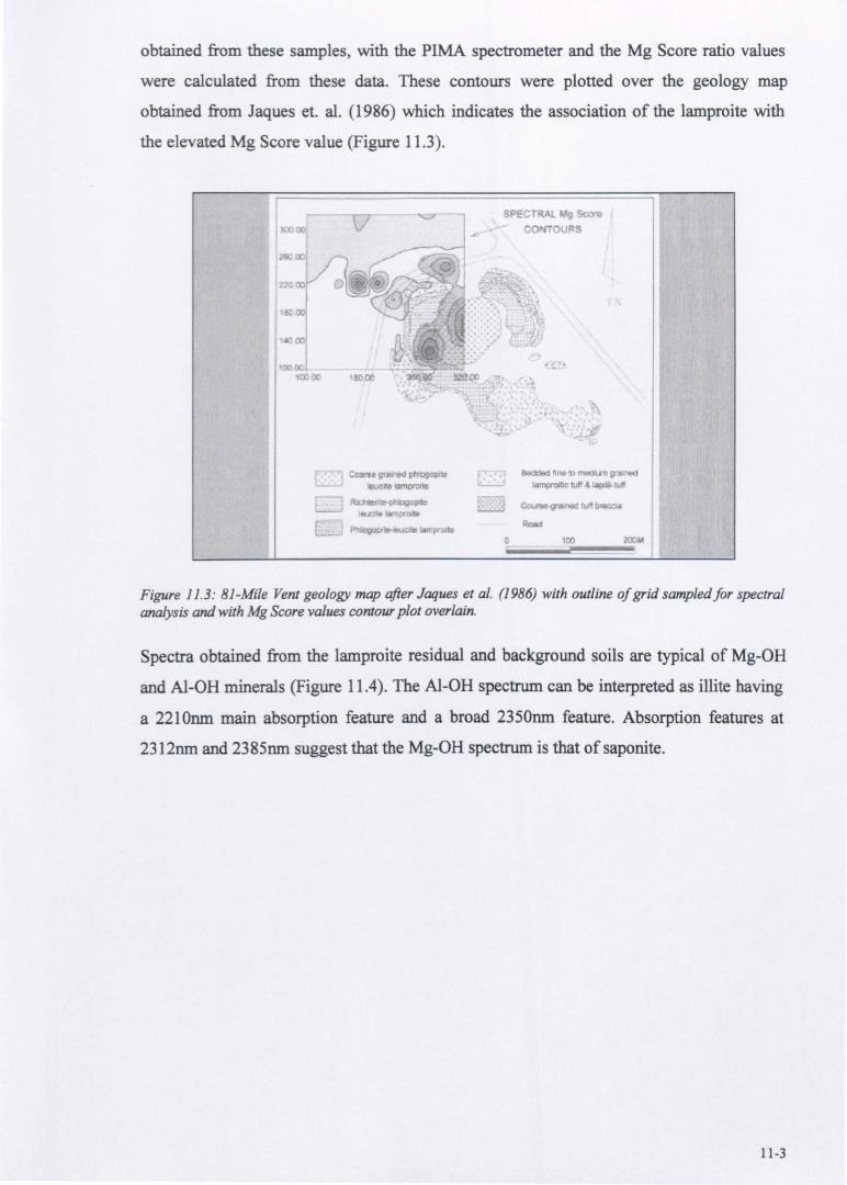
obtained from these samples, with the PIMA spectrometer and the Mg Score ratio values

were calculated from these data. These contours were plotted over the geology map

obtained from Jaques et. al. (1986) which indicates the association of the lamproite with

the elevated Mg Score value (Figure 11.3).

SPECTRA ( <;(""l"9

-- r.ONTOURS

o 100

Figure 11.3: B1-Mile Vent geology map after Jaques et al. (1986) with outline of grid sampled for spectral analysis and with Mg Score values contour plot overlain.

Spectra obtained from the lamproite residual and background soils are typical of Mg-OR

and AI-OR minerals (Figure 11.4). The AI-OR spectrum can be interpreted as illite having

a 2210nm. main absorption feature and a broad 2350nm. feature. Absorption features at

2312nm. and 2385nm. suggest that the Mg-OR spectrum is that of saponite.

11-3

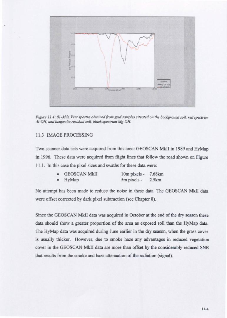
Figure 11.4: B1-Mile Vent spectra obtainedfrom grid samples situated on the background soil, red spectrum AI-On, and lamproite residual soil, black spectrum Mg-OH

11.3 IMAGE PROCESSING

Two scanner data sets were acquired from this area: GEOSCAN MIdI in 1989 and HyMap

in 1996. These data were acquired from flight lines that follow the road shown on Figure

11.1 . In this case the pixel sizes and swaths for these data were:

• GEOSCAN MkII 10m pixels - 7.68km • HyMap Sm pixels - 2.5km

No attempt has been made to reduce the noise in these data. The GEOSCAN MIdI data

were offset corrected by dark pixel subtraction (see Chapter 8).

Since the GEOSCAN MkII data was acquired in October at the end of the dry season these

data should show a greater proportion of the area as exposed soil than the HyMap data.

The HyMap data was acquired during June earlier in the dry season, when the grass cover

is usually thicker. However, due to smoke haze any advantages in reduced vegetation

cover in the GEOSCAN MkII data are more than offset by the considerably reduced SNR

that results from the smoke and haze attenuation of the radiation (signal).

11-4

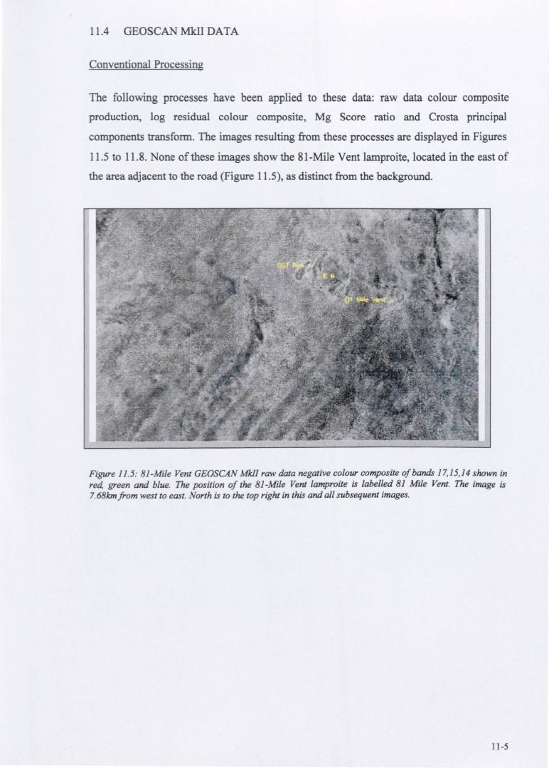
11.4 GEOSCAN MkII DATA

Conventional Processing

The following processes have been applied to these data: raw data colour composite

production, log residual colour composite, Mg Score ratio and Crosta principal

components transform. The images resulting from these processes are displayed in Figures

11.5 to 11.8. None of these images show the 81-Mile Vent lamproite, located in the east of

the area adjacent to the road (Figure 11.5), as distinct from the background.

Figure 11.5: B1-Mile Vent GEOSCAN MkIl raw data negative colour composite of bands 17,15,14 shown in red, green and blue. The position of the 81-Mile Vent lamproite is labelled 81 Mile Vent. The image is 7. 68/an from west to east. North is to the top right in this and all subsequent images.

11 -5

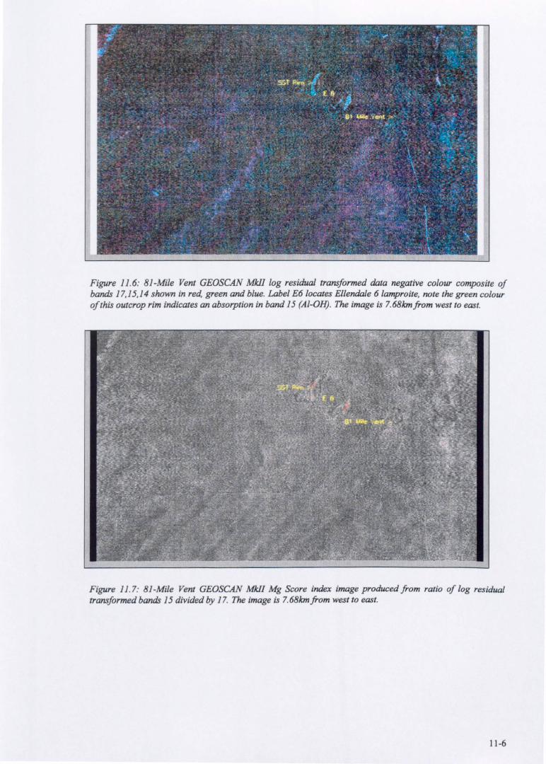
Figure 11.6: 81-Mile Vent GEOSCAN MkIl log residual transformed data negative colour composite of bands 17,15,14 shown in red, green and blue. Label E610cates Ellendale 6lamproite, note the green colour of this outcrop rim indicates an absorption in band 15 (AI-all) . The image is 7. 68kmfrom west to east.

Figure 11.7: 81 -Mile Vent GEOSCAN MJdI Mg Score index image produced from ratio of log residual transformed bands J 5 divided by J 7. The image is 7. 68k:m from west to east.

11-6

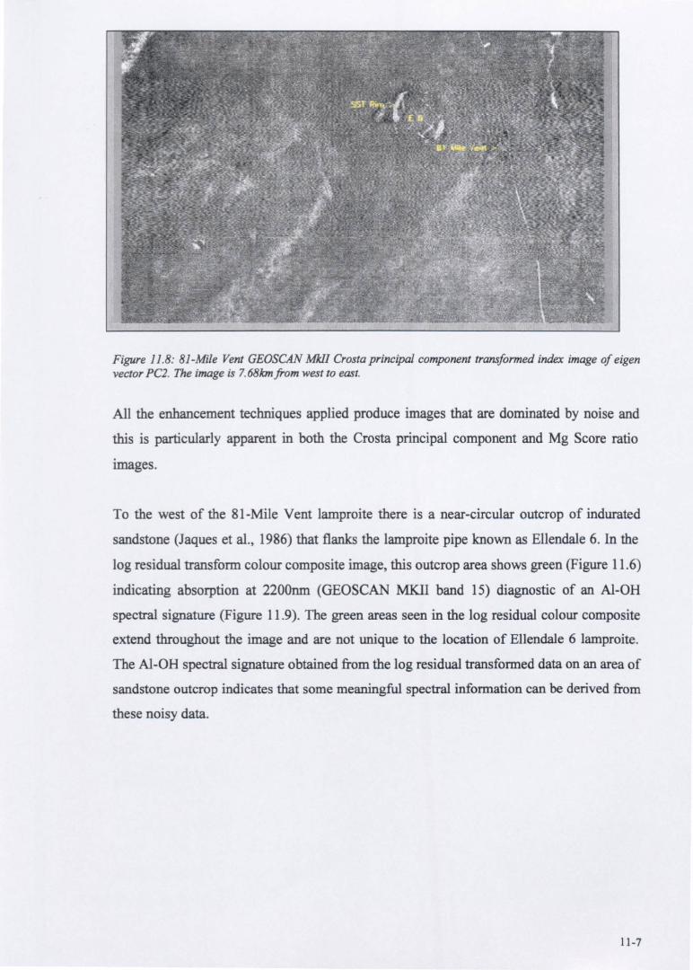
Figure 11.8: 8}-Mile Vent GEOSCAN M1cIJ Crosta principal component transformed index image of eigen vector PC2. The image is 7. 68km from west to east.

All the enhancement techniques applied produce images that are dominated by noise and

this is particularly apparent in both the Crosta principal component and Mg Score ratio

1lllages.

To the west of the 81-Mile Vent lamproite there is a near-circular outcrop of indurated

sandstone (Jaques et al., 1986) that flanks the lamproite pipe known as Ellendale 6. In the

log residual transform colour composite image, this outcrop area shows green (Figure 11.6)

indicating absorption at 2200nm (GEOSCAN MKll band 15) diagnostic of an Al-OH

spectral signature (Figure 11.9). The green areas seen in the log residual colour composite

extend throughout the image and are not unique to the location of Ellendale 6 lamproite.

The Al-OH spectral signature obtained from the log residual transformed data on an area of

sandstone outcrop indicates that some meaningful spectral information can be derived from

these noisy data.

11-7

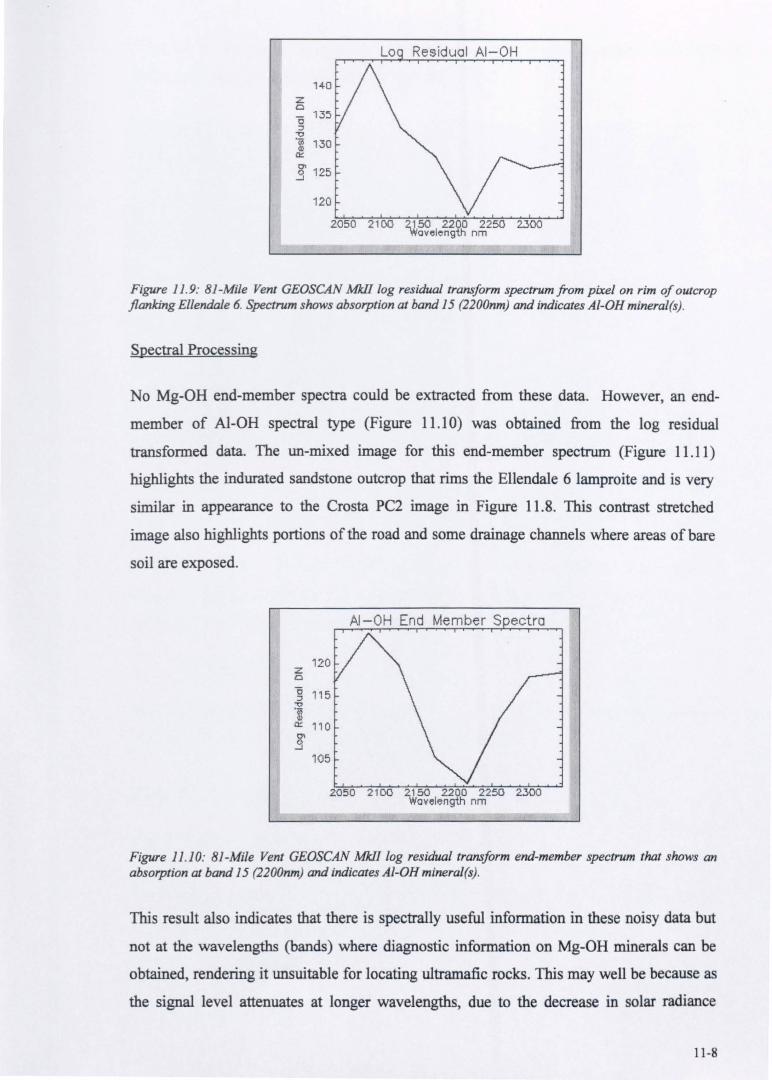
z Cl

140

"0 13:) j

1 130 a::

§ 125

120

2050

Residual AI-OH

Figure 11.9: B1-Mile Vent GEOSCAN MklJ log residual transform spectrum from pixel on rim of outcrop flanking Ellendale 6. Spectrum shows absorption at band 15 (2200nm) and indicates Al-OH mineral(s}.

Spectral Processing

No Mg-OH end-member spectra could be extracted from these data. However, an end­

member of Al-OH spectral type (Figure 11.10) was obtained from the log residual

transformed data. The un-mixed image for this end-member spectrum (Figure 11.11)

highlights the indurated sandstone outcrop that rims the Ellendale 6 lamproite and is very

similar in appearance to the Crosta PC2 image in Figure 11.8. This contrast stretched

image also highlights portions of the road and some drainage channels where areas of bare

soil are exposed.

z Cl

g 115 "0

1 a:: 110

§ 105

Figure 11.10: Bl -Mile Vent GEOSCAN MkIJ log residual transform end-member spectrum thot shows an absorption at band 15 (2200nm) and indicates Al-OH mineral(s}.

This result also indicates that there is spectrally useful information in these noisy data but

not at the wavelengths (bands) where diagnostic information on Mg-OH minerals can be

obtained, rendering it unsuitable for locating ultramafic rocks. This may well be because as

the signal level attenuates at longer wavelengths, due to the decrease in solar radiance

11-8

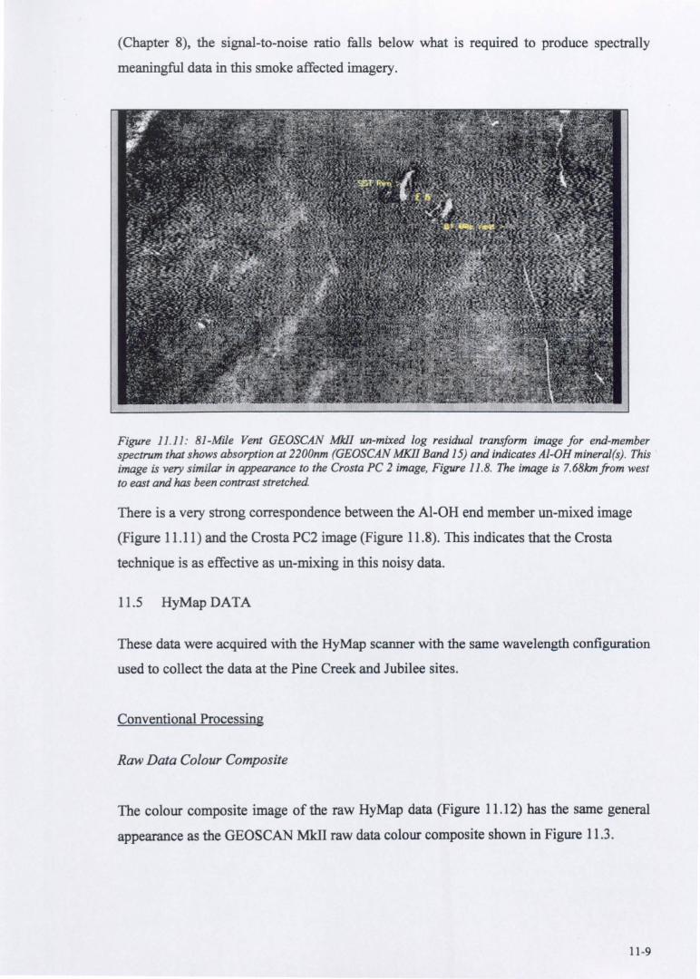
(Chapter 8), the signal-to-noise ratio falls below what is required to produce spectrally

meaningful data in this smoke affected imagery.

Figure 11.11: B1-Mile Vent GEOSCAN Mkll un-mixed log residual transform image for end-member spectrum that shows absorption at 2200nm (GEOSCAN MKJl Band 15) and indicates A/-OH mineral(s). This image is very similar in appearance to the Crosta PC 2 image, Figure J 1.B. The image is 7.6Bkmfrom west to east and has been contrast stretched

There is a very strong correspondence between the AI-OH end member un-mixed image

(Figure 11.11) and the Crosta PC2 image (Figure 11.8). This indicates that the Crosta

technique is as effective as un-mixing in this noisy data.

11.5 HyMap DATA

These data were acquired with the HyMap scanner with the same wavelength configuration

used to collect the data at the Pine Creek and Jubilee sites.

Conventional Processing

Raw Data Colour Composite

The colour composite image of the raw HyMap data (Figure 11.12) has the same general

appearance as the GEOSCAN MkII raw data colour composite shown in Figure 11.3.

11-9

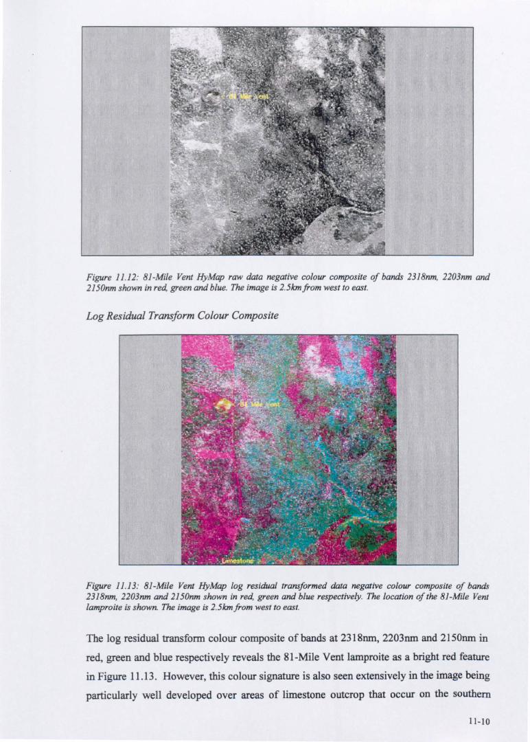
Figure 11.12: 81-Mile Vent HyMap raw data negative colour composite of bands 2318nm, 2203nm and 2150nm shown in red, green and blue. The image is 2. 5km from west to east.

Log Residual Transform Colour Composite

Figure 11.13: 81-Mile Vent HyMap log residual transformed data negative colour composite of bands 2318nm, 2203nm and 2150nm shown in red, green and blue respectively. The location of the 81-Mile Vent lamproite is shown. The image is 2.5kmfrom west to east.

The log residual transform colour composite of bands at 2318nm, 2203nm and 2150nm in

red, green and blue respectively reveals the 81-Mile Vent lamproite as a bright red feature

in Figure 11.13. However, this colour signature is also seen extensively in the image being

particularly well developed over areas of limestone outcrop that occur on the southern

11-10

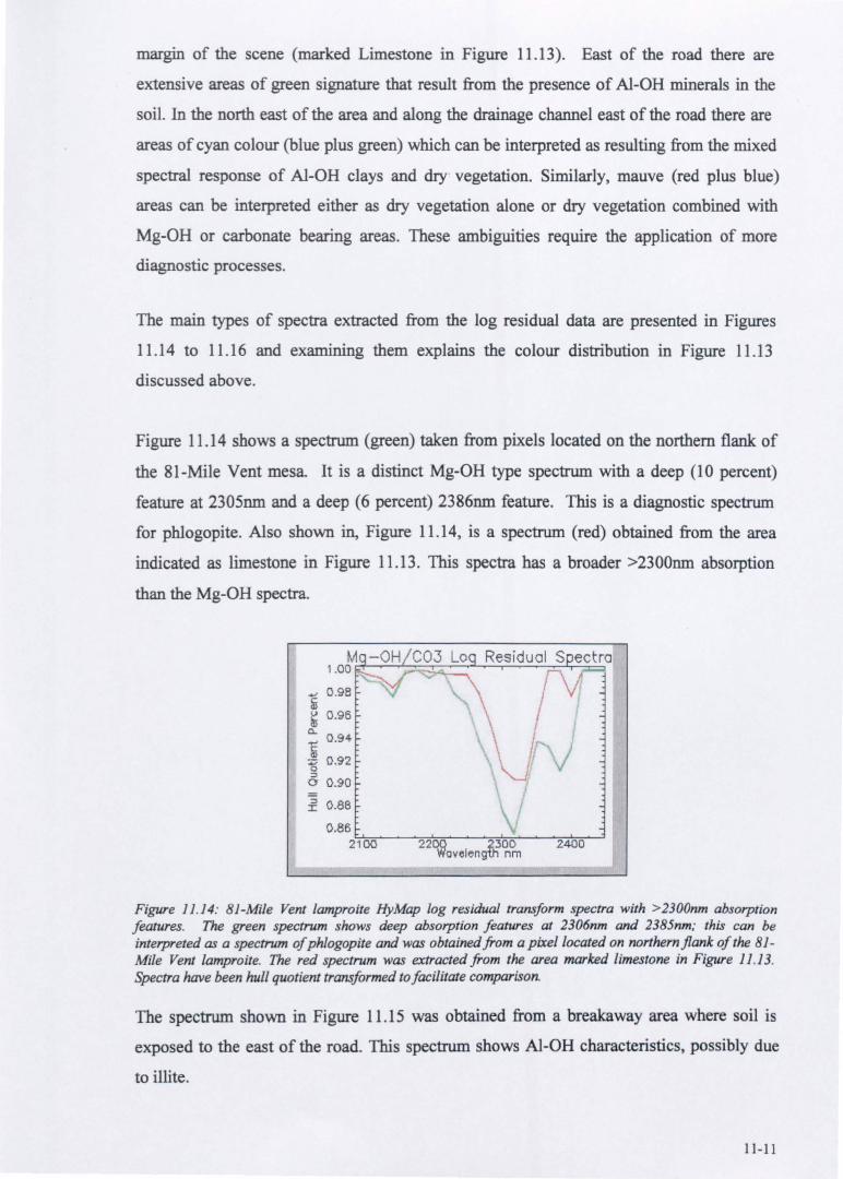
margin of the scene (marked Limestone in Figure 11.13). East of the road there are

extensive areas of green signature that result from the presence of Al-OR minerals in the

soil. In the north east of the area and along the drainage channel east of the road there are

areas of cyan colour (blue plus green) which can be interpreted as resulting from the mixed

spectral response of Al-OR clays and dry' vegetation. Similarly, mauve (red plus blue)

areas can be interpreted either as dry vegetation alone or dry vegetation combined with

Mg-OH or carbonate bearing areas. These ambiguities require the application of more

diagnostic processes.

The main types of spectra extracted from the log residual data are presented in Figures

11.14 to 11.16 and examining them explains the colour distribution in Figure 11.13

discussed above.

Figure 11.14 shows a spectrum (green) taken from pixels located on the northern flank of

the 81-Mile Vent mesa. It is a distinct Mg-OH type spectrum with a deep (10 percent)

feature at 2305nm and a deep (6 percent) 2386nm feature. This is a diagnostic spectrum

for phlogopite. Also shown in, Figure 11.14, is a spectrum (red) obtained from the area

indicated as limestone in Figure 11.13. This spectra has a broader >2300nm absorption

than the Mg-OR spectra .

..., 0 .9 8 5) ~ 0.96 ~ ..... 0.94-c ~ 0.92 o ~

o 0 .90

£ 0.88

0.86 2~1 00~~~2~2~DO~~~2~3~OD~~~~~

Wavel ength nm

Figure 11.14: B)-Mile Vent lamproite HyMap log residual transform spectra with >2300nm absorption features. The green spectrum shows deep absorption features at 2306nm and 2385nm; this can be interpreted as a spectrum of phlogopite and was obtained from a pixel located on northern flank of the 81-Mile Vent iamproite. The red spectrum was extracted from the area marked limestone in Figure 11.)3. Spectra have been hull quotient transformed to facilitate comparison.

The spectrum shown in Figure 11.15 was obtained from a breakaway area where soil is

exposed to the east of the road. This spectrum shows Al-OH characteristics, possibly due

to illite.

11-11

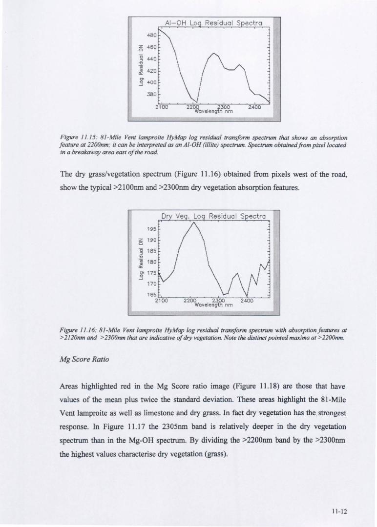
480

t5 460

g 440 -0 'iii ~ 420

.3 400

380

2100

Residual S ectra

Figure 11.15: B1-Mile Vent lamproite HyMap log residual transform spectrum that shows an absorption feature at 2200nm; it can be interpreted as an AI-OH (illite) spectrum. Spectrum obtained from pixel located in a breakaway area east of the road.

The dry grass/vegetation spectrum (Figure 11.16) obtained from pixels west of the road,

show the typical >2100nm and >2300nm dry vegetation absorption features.

195

Z 190 Cl

g 185

1180 a::

8' 175 ..:J

170

Residual S ectra

Figure 11.16: B1-Mile Vent lamproite HyMap log residual transform spectrum with absorption features at >2120nm and > 2300nm that are indicative of dry vegetation Note the distinct pointed maxima at > 2200nm.

Mg Score Ratio

Areas highlighted red in the Mg Score ratio image (Figure 11.18) are those that have

values of the mean plus twice the standard deviation. These areas highlight the 81-Mile

Vent lamproite as well as limestone and dry grass. In fact dry vegetation has the. strongest

response. In Figure 11.17 the 2305nm band is relatively deeper in the dry vegetation

spectrum than in the Mg-OH spectrum. By dividing the >2200nm band by the >2300nm

the highest values characterise dry vegetation (grass).

11-12

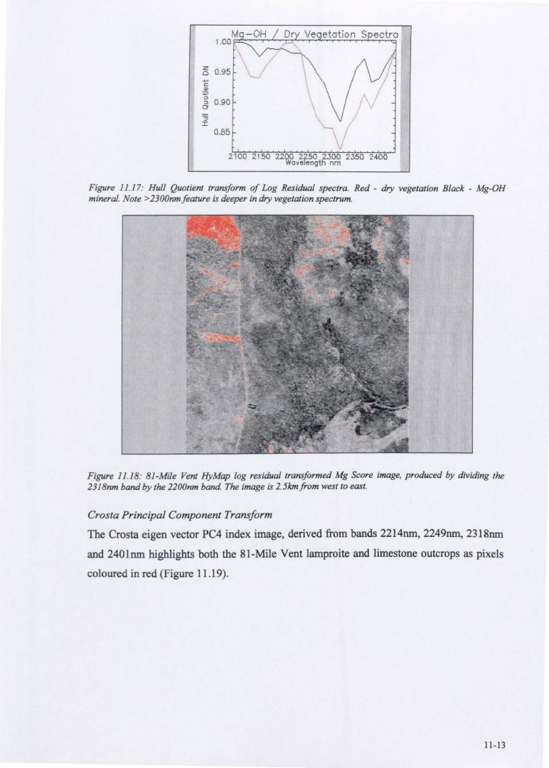
6 Q.95 .... c .s: o <5 0.90

:; I

0.85

2100 2150 2200 2250 2300 2350 2400 Wovelength nm

Figure 11.17: Hull Quotient transform of Log Residual spectra. Red - dry vegetation Black - Mg-OH mineral. Note > 2300nm feature is deeper in dry vegetation spectrum.

Figure 11.1B: B1-Mile Vent HyMap log residual transformed Mg Score image, produced by dividing the 231Bnm band by the 2200nm band The image is 2.5km/rom west to east.

Crosta Principal Component Transform

The Crosta eigen vector PC4 index image, derived from bands 2214nm, 2249nm, 2318nm

and 2401nm highlights both the 81-Mile Vent lamproite and limestone outcrops as pixels

coloured in red (Figure 11.19).

11 -13

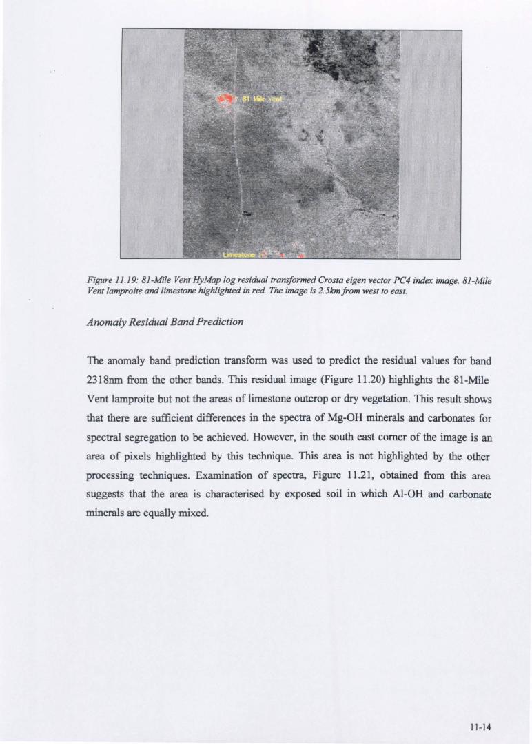
Figure 11.19: B1-Mile Vent HyMap log residual transformed Crosta eigen vector PC4 index image. B1-Mile Vent lamproite and limestone highlighted in red. The image is 2.5kmfrom west to east.

Anomaly Residual Band Prediction

The anomaly band prediction transform was used to predict the residual values for band

2318nm from the other bands. This residual image (Figure 11.20) highlights the 81-Mile

Vent lamproite but not the areas of limestone outcrop or dry vegetation. This result shows

that there are sufficient differences in the spectra of Mg-OH minerals and carbonates for

spectral segregation to be achieved. However, in the south east comer of the image is an

area of pixels highlighted by this technique. This area is not highlighted by the other

processing techniques. Examination of spectra, Figure 11.21, obtained from this area

suggests that the area is characterised by exposed soil in which Al-OH and carbonate

minerals are equally mixed.

11-14

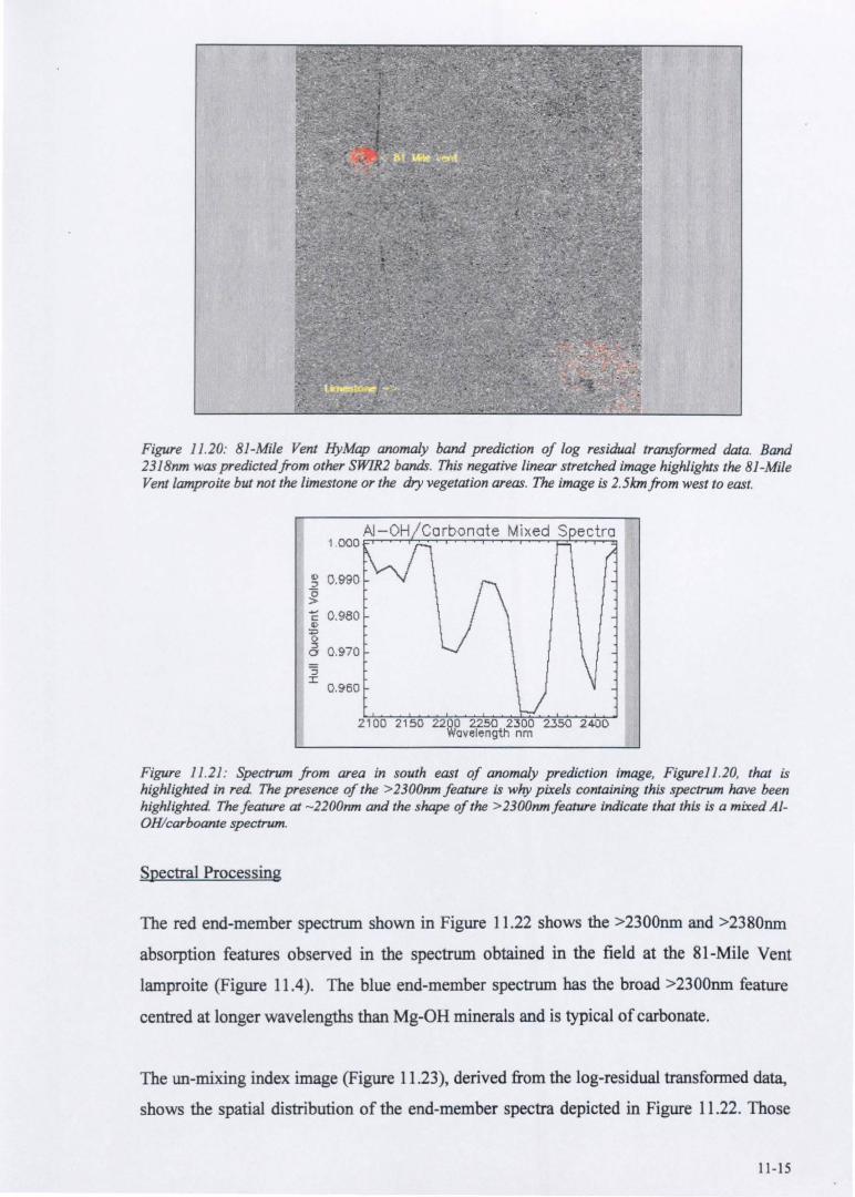
Figure 11.20: B1-Mile Vent HyMap anomaly band prediction of log residual transformed data. Band 231Bnm was predictedfrom other SWIR2 bands. This negative linear stretched image highlights the B1-Mile Vent lamproite but not the limestone or the dry vegetation areas. The image is 2.5kmfrom west to east.

g 0.990 '0 > C 0.980 Q)

g CI 0 .970

0 .960

Figure 11.21: Spectrum from area in south east of anomaly prediction image, Figure1J.20, that is highlighted in red The presence of the > 2300nm feature is why pixels containing this spectrum have been highlighted Thefeature at - 2200nm and the shape of the >2300nmfeature indicate that this is a mixed Al­OHlcarboante spectrum.

Spectral Processing

The red end-member spectrum shown in Figure 11.22 shows the >2300nm and >2380nm

absorption features observed in the spectrum obtained in the field at the 81-Mile Vent

lamproite (Figure 11.4). The blue end-member spectrum has the broad >2300nm feature

centred at longer wavelengths than Mg-OH minerals and is typical of carbonate.

The un-mixing index image (Figure 11.23), derived from the log-residual transformed data,

shows the spatial distribution of the end-member spectra depicted in Figure 11.22. Those

11 -15

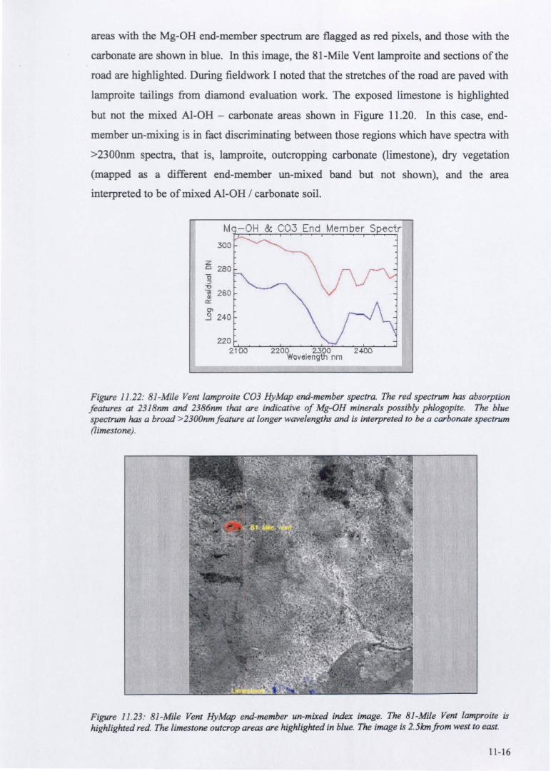
areas with the Mg-OH end-member spectrum are flagged as red pixels, and those with the

carbonate are shown in blue. In this image, the 81-Mile Vent lamproite and sections of the

road are highlighted. During fieldwork I noted that the stretches of the road are paved with

lamproite tailings from diamond evaluation work. The exposed limestone is highlighted

but not the mixed Al-OH - carbonate areas shown in Figure 11.20. In this case, end­

member un-mixing is in fact discriminating between those regions which have spectra with

>2300nm spectra, that is, lamproite, outcropping carbonate (limestone), dry vegetation

(mapped as a different end-member un-mixed band but not shown), and the area

interpreted to be of mixed Al-OH / carbonate soil.

ectr 300

z Cl 280 15 ~

"U 1i 260 a::

.3 240

Figure 11.22: 81-Mile Vent lamproite C03 HyMap end-member spectra. The red spectrum has absorption features at 2318nm and 2386nm that are indicative of Mg-OH minerals possibly phlogopite. The blue spectrum has a broad >2300nmfeature at longer wavelengths and is interpreted to be a carbonate spectrum (limestone) .

Figure 11.23: 81-Mile Vent HyMap end-member un-mixed index image. The 8J-Mile Vent lamproite is highlighted red. The limestone outcrop areas are highlighted in blue. The image is 2.5kmfrom west to east.

11-16

11.6 CONCLUSIONS

The combination of larger pixels, lower spectral resolution and low signal-to-noise ratio

(due to smoke haze) have the effect of severely reducing the effectiveness of GEOSCAN

MldI data for detecting the ultramafic rocks in this area. This may not have been the case

if the data had been acquired at a more optimal time of the year (less smoke) and with

smaller pixels. As is shown in Chapter 10 it should be possible to map the distribution of

materials with >2300nm absorption features with GEOSCAN MKlI data. That this could

not be achieved in this case is therefore a reflection on data quality rather than the system.

As noted in Chapter 10, the Crosta principal component and end-member un-mixing

processes gave virtually identical images for the selected spectral class, Al-OH in this

Chapter and Mg-OH in ChapterlO. This suggests that the lower spectral resolution of the

GEOSCAN MKII data is limiting the amount of unique spectral information to such an

extent that any process that enhances the spectral content will produce the same result.

This is not the case with data having higher spectral resolution such as HyMap. Therefore,

with GEOSCAN MKII and other systems with low spectral resolution, eight or fewer

bands, it is not worthwhile using the more time consuming end-member un-mixing when

the simpler Crosta principal component transform can be applied. However, as the number

of bands increases the problem of which band to select for generating the eigen matrix

becomes more complex. For such data end-member un-mixing will be the preferred

technique to map the location of a particular spectral class.

When the HyMap data is processed using spectral techniques it is possible to differentiate

between spectrally similar minerals, in this case Mg-OH clays, carbonate rocks (limestone)

and dry vegetation, as observed in the Pine Creek investigation (Chapter 9). This

differentiation cannot be achieved with any of the conventional processing techniques

except with the anomaly band prediction process. The spectral processing technique was

the only method tested which unambiguously highlighted the lamproite.

11-17

CHAPTER 12

12 CONCLUSIONS AND RECOMMENDATIONS FOR FURTHER STUDIES

12.1 CONCLUSIONS

The primary objective of this thesis is to demonstrate how spectral geological techniques

can be applied to locate and delineate alkaline ultramafic rocks. Using results obtained

from field spectral studies, with spectrometers and airborne scanner data, I demonstrate

that alkaline and other ultramafic rocks have a diagnostic spectral signature. This signature

can be detected using data obtained from spectrometers, when these rocks are exposed and

weathered into residual soils.

To achieve the detection of ultramafic rocks and probably other rock types consistently,

when exposed and by inference from soils, consistently requires instruments that have

sufficient spectral resolution and a high enough signal-to-noise ratio. It is only within the

last 5 to 7 years that such hyperspectral instruments (field and airborne) have become

available operationally. From this study it is possible to derive a set of specifications that

should be met by an airborne hyperspectral instrument, if it is to be considered for

operational spectral geological investigations.

Airborne scanners such as the HyMap and AVIRIS can and do meet these specifications.

Therefore, it is reasonable for a user to insist that data acquired commercially meets these

specifications, if not the survey should be re-flown or the acquisition cost adjusted

accordingly.

Currently there are no operational hyperspectral spaceborne systems. However, when

considering using data from future systems these specifications can be used as a

benchmark by which to judge the likely utility of data from these systems, for spectral

geological applications.

Non-hyperspectral scanners provide useful spectral data that can be used to discriminate

ultramafic and other rocks but the results are likely to be less definitive and more

ambiguous than that obtained with hyperspectral data. Data from systems such as Landsat

TM, that have broad bands with restricted wavelength coverage, cannot be used to map

12-1

ultramafic rocks consistently. The processing techniques applied to these data, particularly

when utilising the iron oxide information, do not produce consistent results in different

areas. Some idea of a systems potential for discrimination of alkaline (and other)

ultramafic rocks can be determined by comparing its specifications to those listed for

hyperspectral system's below and by referring to Chapter 6.

It can be concluded that to locate alkaline and other ultramafic rocks in an area where they

have not been detected previously requires detecting the Mg-OH spectral signature. This

can only be achieved reliably with data from hyperspectral scanners that meet the

specifications detailed below.

Diagnostic Spectral Signature of Alkaline ultramafic rocks

In this thesis it is established that alkaline and other ultramafic rocks, have a spectral

signature that is derived from minerals that contain Mg-OH. These minerals produce

spectra that have distinct absorption features between 2305nm and 2318nm and near

2385nm in the SWIR2 spectral region. Minerals that have this spectral signature include

serpentine, talc and phlogopite and their weathering product saponite. In this study the

alkaline ultramafic rocks investigated spectrally are kimberlite and lamproite, as well as

other ultramafic rocks, dunite, peridotite and serpentinite and all show the same basic

spectral signature in the SWIR2.

Spectral signature of the weathering products of ultramafic rocks

Ultramafic rocks are altered by hydrolysis and weathering, breaking down into serpentine,

and subsequently Mg-OH bearing smectite clays (saponite). Saponite has a SWIR2

spectrum that is very similar to the primary Mg-OH bearing minerals, therefore, the

diagnostic spectral signature of ultramafic rocks is preserved when these rocks weather

into residual soils. Weathering eventually breaks down saponite into kaolinite, this means

that the residual soils also contain a proportion of AI-OH bearing minerals, as well as

quartz and other minerals introduced into the soil by the erosion of surrounding rocks.

Non Ultramafic Rock Signatures

The diagnostic absorption feature associated with alkaline and other ultramafic rocks near

2300nm can also occur in a variety of other rocks. Either, because they contain minerals

that also have spectral absorption features near 2300nm (such as calcite, dolomite, chlorite

12-2

and certain amphiboles) or the mixture of minerals in the rock can emulate an individual

mineral with a 2300nm feature.

In weathered terrains the presence of several clay minerals such as vermiculite, glauconite

and even kaolinite may produce targets, in the processed image data, due to their spectra

containing a near 2300nm absorption feature.

Applying knowledge of the precise spectra of these confusers to direct the processing

strategy should eliminate most false targets caused by spectral similarities. For example,

using the Mg Score ratio to distinguish areas of kaolinite from saponite. In other cases the

context may permit interpretive grading of anomalies and this may be assisted with

information from other spectral regions. However, there will be cases where targets

selected from imagery will not be spectrally distinguishable from ultramafic rocks even

with field spectra. In such cases only field work will provide a definitive identification. As

experience builds with this technology it is probable that skilled spectral geologists and a

data base of case histories will assist in the correct assignment of spectral anomalies to a

specific rock type or group.

Spectra of Mineral Mixtures

This study has indicated that dilution reduces the intensity of the diagnostic absorption

features proportionally to the amount of Mg-OH clay (saponite) remaining. Experiments

conducted in this study determined that, for binary mixtures, dilution of saponite to 30

percent with minerals and dry vegetation, typically found in soils, still produces a

diagnostic spectrum. The fact that the presence of ultramafic rocks can be detected from

residual soils containing saponite using data collected with field and airborne

spectrometers substantiates the experimental results.

Therefore, such mixing experiments can be used to determine when a mineral being sought

by spectral means will be rendered undetectable due to dilution and/or the masking effects

of other mineral spectra.

Line Scanning Systems Specifications

There are four factors whose specifications determine a scanners ability to deliver

effective data for use in spectral geological applications:

12-3

• Signal-to-Noise Ratio • Spectral Resolution • Pixel Size (or instantaneous field of view) • Pixels per Scan Line (swath width)

Of these the SNR ratio is critical; any modification to the other specifications directly

effects the signal-to-noise ratio. Increasing pixel size will generally improve the signal-to­

noise ratio while increasing spectral resolution will decrease it.

Two other features need to be implemented in a scanning system; the dark current should

be measured for each scan line and the digital data capture should be at least 12 bit.

Other issues that can effect the performance of a scanner system are F number defined by

the optical design, primary mirror design, detector material, detector cooling system and

electronics configuration. These are specialist engineering and optical design areas that

have to be optimised so that the system meets the desired performance specifications.

Signal to Noise Ratio

Investigations carried out into the signal-to-noise ratio of various scanners suggest to me

that an acceptable value is 600:1 at 2200nm from a 50% reflecting surface, for data

delivered from a survey. Which is how the value should be quoted by the systems

manufacturer and/or survey contractor.

A higher noise level can produce spurious absorption features that can result in mis­

identification of the spectral signatures. Noisy image data also result in the targets sought

being obliterated by speckle. The signal-to-noise level decreases with increasing

wavelength due to the marked drop in solar irradiance towards longer wavelengths. This

drop in signal-to-noise ratio is critical when using scanner data to detect ultramafic rocks

because the diagnostic 2300nm absorption feature is located in the longer SWIR2

wavelength spectral region. The Ellendale GEOSCAN MkIl data demonstrated this effect.

Smoke and haze, encountered during the airborne survey reduced the signal. The resultant

reduction in signal-to-noise ratio meant that only the near 2200nm absorption features were

detectable. Consequently only the distribution of AI-OH minerals could be ascertained

with any certainty from these data. The ultramafic target was not detectable in the

GEOSCAN MkII data but it was with the HyMap data, which has a substantially higher

signal-to-noise ratio and spectral resolution. GEOSCAN MkIl scanner data from the

12-4

Jubilee site has a higher signal-to-noise ratio than at 81-Mile Vent and it could be used to

located ultramafic rocks at this site. These results reinforce the importance of noise levels

when evaluating scanner data.

There are ways of reducing noise in the data. The limited study into the effects of noise

showed that with limited spectral resolution systems such as the GEOSCAN MkIl,

applying filters to reduce noise smooths the spectra and shifts the position of absorption

features. Applying these filters can also change overall spectral shapes. This increases the

difficulties of accurately identifying the spectra. With a sufficiently high signal-to-noise

ratio the need for filtering of the data is removed, which is of critical importance when

using these systems operationally. Noise reduction filtering is time consuming and will

adversely effect processing and interpretation times when dealing with the large volumes

of data, typically tens of gigabytes, that these systems produce from large scale surveys

(thousands of square kilometres).

Spectral Resolution

From these studies I conclude that to produce data that can unambiguously identify areas

of ultramafic rocks when exposed and weathered requires a hyperspectral scanner. Such

instruments require SWIR2 bands that of ~ 15nm in width (32 bands covering the spectral

region 2000nm to 2500nm). Typically such an instrument would have between 64 and 96

channels if it recorded data from the VNIR and SWIRl as well.

Narrower bands would probably provide more mineral discrimination but there is an

optical and electronic system trade off between signal-to-noise ratio and spectral

bandwidth (T. Cocks, 1997 pers. comm.). This is an engineering issue. This study showed

that lower signal-to-noise ratio and broader band systems (GEOSCAN Mkil and GER IS)

can produce data from which ultramafic rocks can be delineated, as the Jubilee results

indicate. However, any deterioration in system performance or survey conditions will

render data from such systems useless for this application, as is the case with the Ellendale

GEOSCAN MkII data.

Pixel Size

This issue has not been investigated in this study. A reasonable assumption might be that

the smaller the pixel size the less mixing of the minerals and materials there will be and,

12-5

therefore, the more reliable will be the spectral information derived from the data. In this

study all of the HyMap data was obtained with a 5m pixel. Since these data produced

results consistent with field studies at each test site it can be assumed that 5m is a

satisfactory pixel size.

At the Jubilee site the HyMap scanner produced the most definitive data and also had the

smallest pixel size, 5m compared to the 10m and 15m for the GEOSCAN MkII and GER

scanners respectively. However, since these instruments all have different signal-to-noise

and spectral resolutions these data cannot be used for a meaningful comparison of the

spectral effects of pixel size.

Pixels Per Scan Line

This is an operational consideration. The less pixels per scan line the smaller the swath

width and the greater the number of flight lines and, therefore, the costs of surveying a

given area. Most airborne line scanning systems scan 512 pixels per line, which with 5m

pixels cover an area of2.5 sq km per line km.

Systems (apart from single pixel airborne profiling systems which are not intended for

regional surveys) with less than 512 pixels would probably not now be considered worth

building. Since, survey costs are reduced if the swath width is increased for a given pixel

size, any increase in this specification will be desirable so long as the signal-to-noise ratio

is not compromised.

Dark Current and Digital Quantisation

Scanners such as the GEOSCAN MkII did not measure the dark current during scanning

which makes this fluctuating system offset difficult to remove. This scanner also captured

data with a 7 bit quantisation giving a dynamic range of only 0 to 256. This meant that

offset and gain adjustments were carried out manually during surveys to prevent light and

dark signal saturation. Both of these adjustments need to be removed during data

processing to produce meaningful spectra and this is not always possible.

If the dark current is measured and recorded during the scan cycle its removal becomes a

simple value subtraction from each data value. Increasing the quantisation to 12 bit

12-6

produces a dynamic range of 0 to 4096 which is sufficient to pennit scanning of very

bright and dark targets without the need to apply offsets and adjust the gain of the system.

Summary

A base line scanning system that can reliably detect ultramafic rocks in arid environments

would scan 512 pixels with minimum pixel size of 5m. It would have at least 64 channels

of which 32 would be in the SWIR2. The spectral resolution in the SWIR2 being 15nm per

detector covering the range -2000nm to -2500nm. Other spectrometers would cover the

VNIR and SWIRL The generally broader width of diagnostic absorption features, such as

those related to iron oxides in the NIR, mean that the VNIR and SWIRl spectrometers

could have only sixteen 30nm detectors. The system should be quantised at least 12 bits

and the dark current should be measured during the scan cycle.

The HyMap scanners meet these specifications and this study has demonstrated their

ability to detect alkaline and other ultramafic rocks when exposed and covered by residual

soils in arid areas.

Data Processing Techniques

Once data of sufficient quality have been obtained, it must be processed to extract the

infonnation diagnostic of ultramafic rocks. For spectra obtained from samples collected in

the field, this is straightforward. The Mg Score ratio can be used to detennine values from

spectra that can be contoured or profiled to discriminate between regions of Mg-OH and

AI-OH minerals. When non AI-OH bearing minerals, for example dolomite, are mixed

with Mg-OH minerals other parameters such as the shifts in position of the near 2300nm

absorption feature can be extracted and analysed.

For image data that are not collected as reflectance, processing must commence with the

removal of data offsets, atmospheric effects, the solar irradiance curve and

topographic/albedo variations so that absorption features can be recognised. Correcting the

data for these effects not only assists with visual interpretation of the spectra but also

enhances spectral variations, enabling meaningful values to be extracted from the data. In

this study the log residual transfonn or variations on it such as the ENVI IARR function

have been used to transfonn scanner data to pseudo reflectance. I was able to demonstrate

that this technique is reliable with the data that have been studied. Log residual image

12-7

spectra taken from uniform and homogeneous materials were shown to match the

equivalent spectra collected in the field using the PIMA spectrometer. This similarity is

emphasised when the PIMA spectra are hull quotient transformed.

Of the conventional image processmg techniques applied to detect the location of

ultramafic rocks from scanner imagery the Crosta principle component transform and the

anomaly residual technique provided the most unambiguous results. This was emphasised

when output images from these transforms were clipped to produce index images.

Overall, however, the end-member selection and un-mixing techniques produce the most

consistent results and in two instances, 81 Mile Vent and Pine Creek, were able to

distinguish between different Mg-OH and other minerals showing near 2300nm absorption

features.

Simulated Data

By producing image data simulated from spectra, that is, data cubes it is possible to test the

various processing techniques. Applying conventional processing techniques to modelled

data in this study produced results that do not show the ambiguities produced when real

data is processed. This permitted, for example, the effects of noise on data to be more

easily assessed and how noise effects the different processing techniques abilities to

produce spectrally meaningful images, that is, those in which the targets are highlighted.

Such modelling studies are recommended whenever new processing techniques are being

tested, as it will permit them to be reliably rated against existing techniques. Similarly

variations in spectral resolution and band centres can be tested on simulated data to

determine optimum scanning system parameters.

Simulated mixtures can also be used to determine to what extent minerals can remain

uniquely identifiable spectrally both from field/laboratory spectra and image data. Spectra

of mixed minerals can also be incorporated into image data cubes to test which processing

technique is the most effective at identifying the target mineral.

12-8

Test Site Studies

At the test sites investigated, Mg-OH spectral anomalies are identified by analysis of

samples collected from grids or traverse lines in the field. These anomalies are also

detectable in scanner imaged data collected at these sites. Scanners can record spectra

from a large area within minutes as opposed to days using field spectrometers. Therefore,

in arid to semi-arid areas (where 40 percent of the ground is exposed) scanners are more

effective for conducting regional investigations than are field studies for locating

ultramafic, and by analogy, other rocks

Pine Creek

At the Pine Creek test site the surface soil over the ultramafic rock contains between 60%

and 90% saponite. This value has been obtained by applying the method suggested in

Chapter 7 for estimating the Mg-OH content of mineral mixtures from the Mg Score ratio

value. At this location it is possible to spectrally distinguish soils derived from the

ultramafic rock from the background soils that contain kaolinite and illite.

The results in this study indicate that, even when the minerals of interest are present and

can be identified spectrally, ultramafic rocks may still be confused with other materials in

some circumstances. At Pine Creek in South Australia there appear to be areas of saponite

developed in the soil that may result from the weathering of dolomite (calc-arenite) as well

as that derived from the ultramafic rocks. This indicates that there are limits to using these

methods to locate previously unknown and blind ultramafic rocks.

Jubilee

Data obtained from three scanners (GEOSCAN MkII, GER IS and HyMap) provided

spectral information that mapped the extent of the ultramafic rock at the Jubilee test site.

These data also indicated that unexposed Mg-OH bearing rocks occur to the west of the

main area of ultramafic rock. Spectra recorded in the field mapped mineral variations

within the area of Jubilee ultramafic rock; this difference may be caused by weathering as

the spectra obtained were of serpentine and saponite. This spectral discrimination was

only observed in the HyMap scanner data, which has four times as many SWIR2 bands as

the GEOSCAN MkII and a signal-to-noise ratio that is an order of magnitude better than

the GER IS scanner. Data from these latter two instruments were unable to detect the

12-9

variation in the mineralogy within the Jubilee ultramafic. The smaller pixel size of the

HyMap data may have contributed to the additional discrimination achieved but this aspect

of these data sets was not investigated in this study.

It was only at the Jubilee site that spectral differentiation within exposed ultramafic rocks

was observed. In fact SWIR2 spectra of the various ultramafic rocks are so similar I

consider it unlikely that data from this spectral region alone will be useful in mapping

differences between ultramafic rocks. The studies reviewed in Chapter 2 indicate that it is

possible, using TM data in arid areas, to distinguish differences between ultramafic rocks

spectrally. Most of the spectral variation noted in these studies was attributed to the iron

oxide content of these rocks. I have noted in this study that there are differences in the

VNIR spectral region between alkaline (kimberlite) and other ultramafic rocks but these

differences have not been investigated in detail.

Ellendale

At this site it was confirmed that using end-member un-mixing it is possible to distinguish

exposed alkaline ultramafic rocks from spectrally similar limestone using Hy Map data.

The limitations of the GEOSCAN MkII imaging spectrometer were apparent in data from

this site. Smoke haze had reduced the signal level in the SWIR2 to such an extent that little

meaningful spectral discrimination was possible with these data.

12-10

12.2 RECOMMENDA TIONS FOR FURTHER INVESTIGATIONS

Every study has limits to what can be investigated and ideas for further research are

developed. From the studies completed in this thesis I recommend that the following

topics warrant further research.

• Discriminating between alkaline ultramafic and other ultramafic rocks is economically significant (as kimberlites/lamproites can have a significant diamond content). The use of spectral geological techniques for this purpose requires further investigation. This, and other studies, have indicated that the VNIR spectral region may contain spectral information that can be used for this discrimination once the ultramafic rock has been located from the SWIR2 spectral signature. Further research on this topic requires spectral data from areas where these rock types are in juxtaposition.

• In arid areas that have been subjected to a previous phase of intense lateritic weathering the typical clay mineral weathering products of serpentinised ultramafic rocks may have been replaced by ferruginous silicified saprolite (silcrete). This material has a diagnostic SWIR2 spectra with a broad shallow absorption feature near 2240nm. Therefore, a study (using the methods detailed in this thesis) to determine if this spectral signature can be used to locate ultramafic rocks is warranted.

• The end-member un-mixing routines in ENVI work but they require streamlining and developing into an automated package for routine processing of operationally acquired data.

• The effect of noise filtering on hyperspectral data requires further study. Distortion of the spectral form can result from filtering. Therefore, there is a trade-off between noise reduction and maintaining spectral resolution. Hence the type and optimum level of filtering that successfully removes noise but does not degrade the diagnostic spectral information needs to be established. This requires developing a program or programs that can accurately estimate the signal-to-noise level from the data directly.

• Atmospheric corrections based on ATREM and other atmospheric models (Clarke et aI., 1994) are becoming more accessible but they rely on input of generalised atmospheric parameters that may be different to the model on the survey day. These techniques are particularly important when working with the VNIR where atmospheric offsets are more severe than in the SWIR2. The log residual transform was used to convert radiance data to pseudo reflectance in this study but it does not produce reliable results when applied to VNIR data. Furthermore, if the scene contains significant amounts of the material of interest the log residual transform can produce spurious results. Therefore, experiments to determine the level at which the percent of ultramafic rock in a scene will cause this problem are required. Techniques should be developed which correct the scanner data from the spectral variations within it, without the need to develop atmospheric models.

12-11

• This research suggested that variations in image pixel size could affect the results obtained. At the Jubilee site where variations in pixel size occurred they resulted from different instruments and so this aspect of system characteristics could not be adequately investigated. This study should be conducted using real data rather than simulated data from mathematical models. It is suggested that the Jubilee and/or Pine Creek sites be resurveyed with the HyMap scanner to obtain a range of pixel sizes from 3m to 20m. From such data sets it would be possible to determine how pixel size actually affects the ability of these data to spectrally discriminate ultramafic rocks. This would also have generic implications for all remote sensing systems.

• This research has demonstrated that it is possible to locate alkaline and other ultramafic rocks. However, the possibility that saponite, an important mineral in achieving this in soil covered areas, can also be produced by the weathering of dolomite requires investigation. It needs to be determined whether such saponite formation results from hydrothermal alteration or from a weathering phenomenon. The Pine Creek area of South Australia would be an ideal site to commence such a study.

12-12

GLOSSARY OF TERMS AND ACRONYMS Arid

ATREM

AVIRIS Bands (Channels)

Crosta technique

A climate characterised by dryness variously defined as rainfall insufficient for plant life or crops without irrigation; less than 25cms of annual rainfall or higher evaporation rate than precipitation rate. Atmosphere Removal Program - program developed at University of Colorado that converts airborne scanner radiance values to reflectance percent. Airborne Visible/Infrared Imaging Spectrometer. The interval over which a spectrometer samples the spectrum The larger the number over a defined range the greater the spectral resolution of the instrument. A method of applying principal component transforms to image data so that regions which contain a diagnostic absorption feature are highlighted. Four bands are input to the transform, one in which the absorption feature of interest is located and three reference bands. Examination of the Eigen matrix for these bands shows which Eigen vector has the weights which will result in a transformed image that highlights the absorption feature of interest.

End-member A spectrum in a series of spectra collected from the field samples or

GER Hull Difference

image pixels that are unique and represent one pure mineral type. Geophysical Environmental Research Company. Value obtained by subtracting the Y-axis values of a spectrum from the Y-axis values of a line constructed as a hull across the apex of all peaks along the spectrum. It is expressed as a percentage and permits detection of the relative depths of the absorption features that is emphasises.

Hull Quotient Value obtained by dividing the Y-axis values of a spectrum into the Y­xis of a line constructed as a hull across the apex of all peaks along the spectrum. It is expressed an as a percentage and removes the

HyMap background spectral curve so emphasising absorption features. Trade mark for a range of hyperspectral scanners produced by Integrated Spectronics.

Hyperspectral A scanner that has more than 24 bands that are contiguous Scanner within wavelength regions VNIR, SWIRl and SWIR.2 Imaging Usually taken as synonymous with hyperspectral scanner, in this study Spectrometer defined as scanners that have between 8 and 24 bands that are

Mg Score ratio

Multispectral Scanner (MSS)

contiguous within wavelength regions. The value obtained from dividing the Y-axis value of a spectrum at 2300nm by the value at 2200nm. When obtained from field spectra this ratio value can be plotted to delineate the extent of Mg-OH compared to AI-OH minerals. The ratio is usually calculated from hull quotient transformed spectra. This term can also be used to specify the image ratio obtained by dividing the scanner image bands at these wavelengths data. An imaging scanner that has limited bands. In this study less than eight that are not contiguous. These instruments under sample the spectrum.

PIMA

Semi Arid

SWIRl SWIR2 Un-mixing

VNIR

Portable Infrared Mineral Analyser. SWIR field spectrometer produced by Integrated Spectronics. Type of climate in which there is slightly more precipitation 2S-S0cms than in arid climate and in which sparse grasses are the characteristic vegetation. Short Wave Infra red spectral region from 1200nm-2000nm Short Wave Infra red spectral region from 2000nm-2S00nm Techniques used to calculate the proportions of end-member spectrum that are combined in the spectra of a mineral mixture. These techniques can be applied to image data to map the spatial distribution of various minerals and materials from their spectral signatures. Visible to Near Infra red spectral region from 400nm-1200nm

2

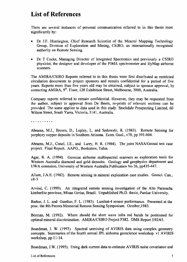
List of References

There are several instances of personal communication referred to in this thesis most significantly by:

• Dr IF. Huntington, Chief Research Scientist of the Mineral Mapping Technology Group, Division of Exploration and Mining, CSIRO, an internationally recognised authority on Remote Sensing.

• Dr T Cocks, Managing Director of Integrated Spectronics and previously a CSIRO physicist, the designer and developer of the PIMA spectrometer and HyMap airborne scanners.

The AMIRAICSIRO Reports referred to in this thesis were first distributed as restricted circulation documents to project sponsors and remain confidential for a period of five years. Reports more than five years old may be obtained, subject to sponsor approval, by contacting AMIRA, 9th

• Floor, 128 Exhibition Street, Melbourne, 3000, Australia.

Company reports referred to remain confidential. However, they may be requested from the author, subject to approval from De Beers, re-prints of relevant sections can be provided. The same applies to data used in this study. Stockdale Prospecting Limited, 60 Wilson Street, South Yarra, Victoria, 3141, Australia.

Abrams, MJ., Brown, D., Lepley, L. and Sadowski, R. (1983). Remote Sensing for porphyry copper deposits in Southern Arizona. Econ. Geol., v78, pp 591-604.

Abrams, MJ., Conel, J.E., and Larry, H. R. (1984). The joint NASAIGeosat test case project. Final Report. AAPG., Bookstore, Tulsa.

Agar, R. A. (1994). Geoscan airborne multispectral scanners as exploration tools for Western Australia diamond and gold deposits. Geology and geophysics department and UWA extension, University of Western Australia Publication No 26, pp435-447.

Allum, J.A.E. (1982). Remote sensing in mineral exploration case studies. Geosci. Can., v8-3

Arvind, C. (1990). An integrated remote sensing investigation of the Alto Paranaiba kimberlite province, Minas Gerias, Brazil. Unpublished Ph.D. thesis, Purdue University.

Barker, J. L. and Gunther, F. L. (1983). Landsat-4 sensor performance. Presented at the proc. the 8th Pecora Memorial Remote Sensing Symposium. October, 1983.

Berman, M. (1992). Where should the short wave infra red bands be positioned for optimal mineral discrimination. AMlRAlCSIRO Project P382. DMS Report E92/65.

Boardman, J. W. (1993). Spectral unmixing of AVIRIS data using complex geometry concepts. Summaries of the fourth annual JPL airborne geoscience workshop. vI AVIRIS workshop, pp 11-14.

Boardman, J.W. (1995). Using dark current data to estimate AVIRIS noise covariance and

List of References

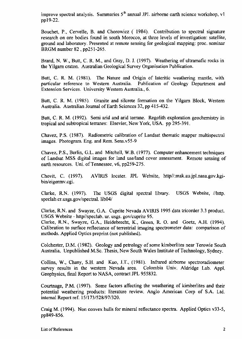
improve spectral analysis. Summaries 5th annual JPL airborne earth science workshop, vI ppI9-22.

Bouchet, P., Cervelle, B. and Chorowicz (1984). Contribution to spectral signature research on ore bodies found in south Morocco, at three levels of investigation: satellite, ground and laboratory. Presented at remote sensing for geological mapping: proc. seminar BRGM number 82, pp251-265.

Brand, N. W., Butt, C. R. M., and Gray, D. 1. (1997). Weathering of ultramafic rocks in the Yilgam craton. Australian Geological Survey Organisation Publication.

Butt, C. R. M. (1981). The Nature and Origin of lateritic weathering mantle, with particular reference to Western Australia. Publication of Geology Department and Extension Services. University Western Australia., 6.

Butt, C. R. M. (1985). Granite and silcrete formation on the Yilgam Block, Western Australia. Australian Journal of Earth Sciences 32, pp 415-432.

Butt, C. R. M. (1992). Semi arid and arid terrane. Regolith exploration geochemistry in tropical and subtropical terranes: Elsevier, New York, USA. pp 295-391.

Chavez, P.S. (1987). Radiometric calibration of Landsat thematic mapper multispectral images. Photogram. Eng. and Rem. Sens.v55-9

Chavez, P.S., Berlin, G.L. and Mitchell, W.B. (1977). Computer enhancement techniques of Landsat MSS digital images for land use/land cover assessment. Remote sensing of earth resources. UnL of Tennessee, v6, pp259-275.

Chovit, C. (1997). AVIRIS locater. JPL Website, http//:mak.au.jpl.nasa.gov.kgi-binleigermv.cgi.

Clarke, R.N. (1997). The USGS digital spectral library. USGS Website, //http. speclab.cr.usgs.gov/spectral. lib041

Clarke, R.N. and Swayze, G.A. Cuprite Nevada AVIRIS 1995 data tricorder 3.3 product. USGS Website - http//spec1ab. ur. usgs. gov/cuprite 95. Clarke, R.N., Swayze, G.A., Heidebrecht, K., Green, R. o. and Goetz, A.H. (1994). Calibration to surface reflectance of terrestrial imaging spectrometer data: comparison of methods. Applied Optics preprint (not published).

Colchester, D.M. (1982). Geology and petrology of some kimberlites near Terowie South Australia. Unpublished M.Sc. Thesis, New South Wales Institute of Technology, Sydney.

Collins, W., Chany, S.H. and Kuo, J.T., (1981). Infrared airborne spectroradiometer survey results in the western Nevada area. Colombia Univ. Aldridge Lab. Appl. Geophysics, final Report to NASA, contract JPL 955832.

Courtnage, P.M. (1997). Some factors affecting the weathering of kimberlites and their potential weathering products: literature review. Anglo American Corp of S.A. Ltd. internal Report ref: 15/173/528/97/320.

Craig M. (1994). Non convex hulls for mineral reflectance spectra. Applied Optics v33-5, pp849-856.

List of References 2

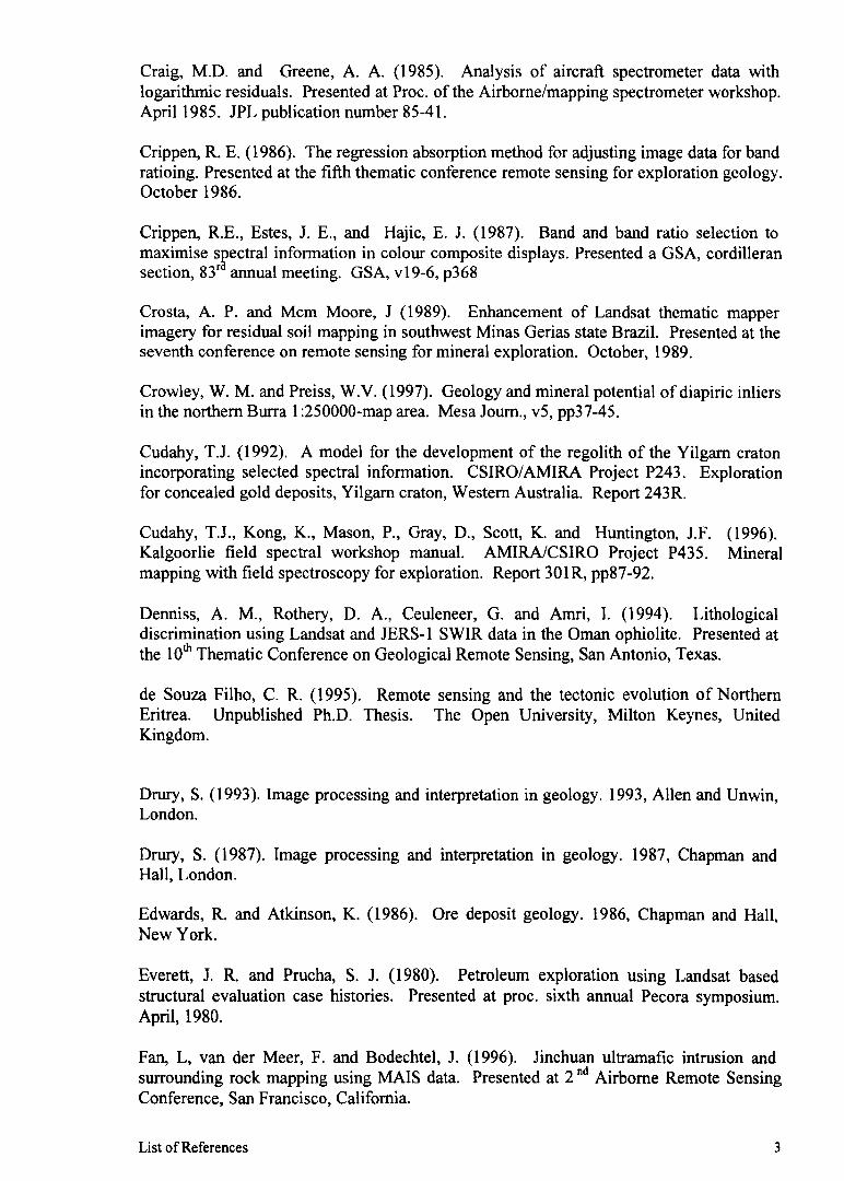
Craig, M.D. and Greene, A. A. (1985). Analysis of aircraft spectrometer data with logarithmic residuals. Presented at Proc. of the Airborne/mapping spectrometer workshop. April 1985. JPL publication number 85-41.

Crippen, R. E. (1986). The regression absorption method for adjusting image data for band ratioing. Presented at the fifth thematic conference remote sensing for exploration geology. October 1986.

Crippen, R.E., Estes, J. E., and Hajic, E. J. (1987). Band and band ratio selection to maximise sfectral information in colour composite displays. Presented a GSA, cordilleran section,83 f annual meeting. GSA, v19-6, p368

Crosta, A. P. and Mcm Moore, J (1989). Enhancement of Landsat thematic mapper imagery for residual soil mapping in southwest Minas Gerias state Brazil. Presented at the seventh conference on remote sensing for mineral exploration. October, 1989.

Crowley, W. M. and Preiss, W.V. (1997). Geology and mineral potential of diapiric inliers in the northern Burra 1 :250000-map area. Mesa Journ., v5, pp37-45.

Cudahy, T.J. (1992). A model for the development of the regolith of the Yilgarn craton incorporating selected spectral information. CSIRO/AMlRA Project P243. Exploration for concealed gold deposits, Yilgarn craton, Western Australia. Report 243R.

Cudahy, T.J., Kong, K., Mason, P., Gray, D., Scott, K. and Huntington, 1.F. (1996). Kalgoorlie field spectral workshop manual. AMlRAlCSIRO Project P435. Mineral mapping with field spectroscopy for exploration. Report 301R, pp87-92.

Denniss, A. M., Rothery, D. A., Ceuleneer, G. and Amri, I. (1994). Lithological discrimination using Landsat and JERS-l SWIR data in the Oman ophiolite. Presented at the 10th Thematic Conference on Geological Remote Sensing, San Antonio, Texas.

de Souza Filho, C. R. (1995). Remote sensing and the tectonic evolution of Northern Eritrea. Unpublished Ph.D. Thesis. The Open University, Milton Keynes, United Kingdom.

Drury, S. (1993). Image processing and interpretation in geology. 1993, Allen and Unwin, London.

Drury, S. (1987). Image processing and interpretation in geology. 1987, Chapman and Hall, London.

Edwards, R. and Atkinson, K. (1986). Ore deposit geology. 1986, Chapman and Hall, New York.

Everett, 1. R. and Prucha, S. 1. (1980). Petroleum exploration using Landsat based structural evaluation case histories. Presented at proc. sixth annual Pecora symposium. April, 1980.

Fan, L, van der Meer, F. and Bodechtel, J. (1996). Jinchuan ultramafic intrusion and surrounding rock mapping using MAIS data. Presented at 2 nd Airborne Remote Sensing Conference, San Francisco, California.

List of References 3

Fergusson, 1. and Sheraton, 1. W. (1979). Petrogenesis of kimberlitic rocks of southeastern Australia. Proc. second international kimberlite conference, 1997 - proceedings, 1979.

Fraser, SJ. (1985). Discrimination of iron oxides and vegetation anomalies with MEIS narrow band imaging system. Presented at fourth thematic conference remote sensing for exploration geology. April, 1985.

Fuliganati, P., Malfitano, G. and Sbrana, A. (1997). The pantelleria caldera geothermal system: Data from hydrothermal minerals. Journ. of vulcanology and geothermal res., v75, pp251-270.

Gabell, A. R. (1986). High resolution remote sensing apply to Mineral Exploration in Australia. Unpublished Ph.D. thesis, Adelaide University.

Gabell, A. R., Huntington, J. F., Green, A. A. and Craig, M. (1983). Interpretation of high resolution airborne visible and near infrared spectroradiometer data from the Kambalda region, W. A. AMIRA investigation Report 1484R. Project 791, P112C.

Gabell, A. R., Huntington, J.F., Green, A. A. and Craig, M. (1983). Interpretation of high resolution airborne visible and near infrared spectroradiometer data over the Mt Turner porphyry copper system, Georgetown, Queensland. AMIRA investigation Report 1454R. Project 791, p112C.

Gentilli, J. (1997). Climate, in Jeans (ed). The natural environment. 1977, Sydney University Press, Sydney.

Gonzalez, R. E. and Winz, P. (1987). Digital Imaging Processing. 1987, Addison Wesley, Reading.

Graham, J. (1967). Formulation of saponite from kaolinite, quartz and dolomite. Amer. Mineralogist, v52, pp1560-1561.

Green, R. O. (1993). Summaries of the fourth annual JPL airborne geoscience workshop. October 1993. vI AVIRIS Workshop. NASA publication number 93-26.

Grim, R. E. (1968). Clay mineralogy. 1968, McGraw Hill, New York.

Harding, D. J. and Bird, J. M. (1984). Mapping ultramafic rock using Landsat MSS. The Josephine peridotite, Oregon. Presented at the International Symposium on remote sensing of environment. 3rd Thematic Conference, remote sensing for exploration geology, Colorado Springs, Colorado.

Hawthorne, lB. (1975). Model ofa kimberlite pipe. Phys. Chern. of the Earth. v9, ppl-15.

Hlvaku, C. (1987). De-striping AIS using fourier filtering techniques. Proc. second AIS data analysis workshop. JPL Pub 86-35, pp74-80.

Honey, F. R. and Daniels, J. L (1986). Rock discrimination and alteration mapping for mineral mapping using the Carr BoydJGEOSCAN airborne multispectral scanner. Presented at the fifth ERIM thematic conference: remote sensing for exploration geology. September, 1986.

List of References 4

Hook, S.J., Elvidge, C. D., Rast, M. and Watanabe, H. (1990). An evaluation of SWIR data from the A VIRIS and Geoscan Instruments for mineralogical mapping at cuprite Nevada. Geophysics, v56-9, pp1432-l440.

Hunt, G. R., Salisbury, J.W. (1976). Visible and near infra red spectra of minerals and rocks: XII Metamorphic Rocks. Modem Geology, v5, pp2l9-228.

Huntington, J. F., Boardman, J., Craig, M. D., Munday, J.1. and Gabell, A. R. (1994). Mineral mapping with spectrally processed GEOSCAN MkII scanner data: Copper Gorge, Nullagine, Western Australia. AMIRAICSIRO Project P382, Report 46R.

Huntington, J. F., Cudahy, J. J., Craig, M. D. and Mason, P. (1994). Mineral mapping with spectrally processed GEOSCAN MklI scanner data, Olary district. South Australia., AMIRICSIRO Project P382. Report 45R.

Hussey, M. C. (1986). Application of remote sensing imagery in defining area for heavy mineral sampling in the Yilgarn. Presented at proceedings second international conference on prospecting in arid terrain. April, 1988.

Hussey, M. C. and Hunt, G.A (1990). Variations on the Abrams ratios for mapping clay, iron and vegetation with TM imagery. Presented at the fifth Australian remote sensing conference. October, 1990.

Jackson, D. G. and Haebig, A. E. (1997). Geochemical expression of some west Australian kimberlites and lamproites. Presented at fourth international kimberlite conference. August, 1986.

Jackson, J.A. (1997). Glossary of geology. 1997, American Geological Institute, Alexandria.

Jaques, A. L., Lewis, J.D. and Smith, C. B. (1986). The kimberlites and lamproites of Western Australia. 1986, Dept of Mines, Western Australia, Bulletin 132, Perth.

Joyce, J., Arculus, R. J. and Ferguson, J (1982). Kimberlite and kimberlite intrusives of southeastern Australia: a review. BMR journal of Australian geology and geophysics, v4, pp227-241.

Kersten, P. (1973). Differential analysis of kimberlites. In Nixon, P. H. (ed). Lesotho Kimberlites. 1973, Lesotho NDC, Maseru.

Kramer, H. J. (1994). Observation of the Earth and its Environment. Springer and Verlag, Berlin, Germany.

Kruse, F. A. and Huntington, J. F. (1996). The 1995 AVIRIS geology group shoot Presented in summaries of annual JPL workshop v4, 1996 AVIRIS Workshop ppI55-162.

Kruse, F.A. and Boardman, J.W. (1997). Characterisation and mapping ofkimberlites and related diatremes in Utah, Colorado and Wyoming, USA, using the airborne visible/infrared imaging spectrometer (AVIRIS). Presented in the twelfth international conference and workshops on applied geologic remote sensing. November, 1997.

List of References 5

Lewis, M. (1996). Pine Creek Vegetation Study. 1996 Unpublished Report for Stockdale Prospecting Ltd.

Loughlin, W. P. (1991). Principal component analysis for alteration mapping. Presented at the eighth symposium of geologic remote sensing. May 1991 .

Lyon, R. J. P. (1990). Effects of weathering, desert varnish, etc. on spectral signatures of mafic, ultramafic and felsic rocks, Leonora, Western Australia. IGARSS '90. Remote Sensing Science for the Nineties 10, pp 1719-1722.

Lyon, R. J. P. (1964). Evaluation of infra red spectrophotometry for composition analysis of lunar and plant soils. Stanford Research Institute Project no. PHU-3943, final Report order contact no. NASA TND-1871.

Lyon, R. J. P., Tuddenham, W.M. and Thompson, C.S. (1959). Quantitative Mineralogy in 30 minutes. Econ. Geol., v54, p1047.

Macias, L.F. (1995). Remote sensing of mafic-ultramafic rocks: examples from Australian precambrian terranes. AGSO Journ. of Australian geology and geophysics, v16, pp163-171.

Marsh, S. E. and McKeon, J. B. (1983). Integrated Analysis of high-resolution field and airborne spectroradiometer data for alteration mapping. Econ. Geol., v78, pp618-632.

Mather, P. M. (1987). Computer processing of remotely sensing images. 1987, John Wiley, Chichester.

Mclaughlin, R. (1984). XRD analysis of clay minerals from the Terowie area, South Australia. Unpublished Report to Stockdale Prospecting.

McMaster, R A and Marx, M. R.(1984). E5 Jubilee: termination Report. Stockdale Prospecting internal Report.

Middlemost, A. K. (1985). Magmas and magnetic rocks. Longman, London.

Mitchell, R. H. (1970). Kimberlites and related rocks - a critical reappraisal. Journal of Geology 78. pp686-704.

Mitchell, R. H. (1986). Kimberlites. Plenum Press, London.

Mitchell, R. H. (1986). Aspects of the petrology of kimberlites and lamproites. In kimberlites and related rocks, 1986 Geological Soc. of Australia special publication no.14. Blackwell, Oxford.

Mitchell, R. H. (1995). Kimberlites, organgeites and related rocks. Plenum Press, London.

Mitchell, R. H. and Berryman, S. C. (1991). Petrology of lamproites. Plenum Press, London.

Mustard, J. F. and Pieters, C. M. (1986). Abundance and distribution of mineral components associated with the Moses Rock (kimberlite)

List of References 6

Mustard, 1. F. and Pieters, C. M. (1988). Application of imaging spectrometer data to the Kings-Kaweah ophiolite melange. Proc. second AIS data analysis workshop. JPL Pub 86-38, pp122-127.

OConnor, E. A (1993). Mapping metamorphism with Landsat TM. in the Arabian Shield, Eastern Egypt. Presented at the 9 tit Thematic Conference on geologic remote sensing. Pasadena, Arizona

Ollier, C. D. Chan, R. A and Craig, M. A (1988). Aspects of landscape history and regolith in the Kalgoorlie Region, Western Australia. BMR Journal of Australian Geology and Geophysics 10. pp309-321.

Ollier, C. D. and Pain, C. R. (1996). Regolith, Soils and Landforms. John Wiley and Sons, Chichester, UK.

Pendock, N. E. and Lamb, A (1989). Band prediction technique for the mapping of hydrothermal alterations. Presented at the seventh thematic conference on remote sensing for exploration geology. October, 1989.

Pontual, A (1990). Lithological information in remotely sensed images and surface in arid regions. Unpublished Ph.D. Thesis, Open University.

Pontual, A. (1995). Detailed analysis of kaolinised kimberlite from the Seppelt kimberlite: infrared, X-ray diffraction and stable isotopes. Unpublished Report to Stockdale Prospecting.

Pontual, A, Merry N and Gamson, P. (1997). Spectral analysis guides for mineral exploration v5. Near surface weathering environments. 1997, AusSpec International, Melbourne.

Post, J. L. (1984). Saponite from near Ballarat, California. Clay and Clay minerals v32-2. ppI47-153.

Potter, J. F. (1977). The correction of Landsat data for the effects of haze and sun angle background reflectance. Presented at proc. on machine processing of remotely sensed data. 1977, Purdue University, pp24-32.

Potter, W. M., Orien, T. G., Hansen, A. M. (1990). Evolution of the AVIRIS. Flight and ground data processing systems. SPIE, v1298, p11-17.

Ramsey, M. S. and Christensen, P. R. (1998). Mineral abundance determination: quantitative deconvolution of thermal emission spectra. Journ. Geophy. Res., v103, pp577-596.

Richards, J. A. (1986). Remote Sensing Digital analysis. 1986, Springer - Verlag, Berlin.

Rivand, B. (1989). Mapping ophiolitic melanges of the central eastern desert of Egypt using a linear mixing model applied to Landsat thematic mapper data. Presented at the seventh thematic conference on remote sensing for exploration geology. October, 1986.

Ross, J. (1986). Kimberlites and related rocks. 1986, GSA special pUblication no. 14, vI

List of References 7

Rothery, D. A (1982). Supervised maximum likelihood classification and post­classification filtering using MSS imagery for lithological mapping in the Oman ophiolite. Presented at the proc. of the int. symp. on remote sensing of environment, second thematic conference. December 1982.

Rowan, L. C., Goetz, A.G.H. and Ashley, R.P. (1977). Discrimination of hydrothermally altered and unaltered rocks in visible and near infra red multi-spectral images. Geophysics, v42, pp522-535. Rowan, L. c., Bowers, L., Crowley, J. K., Pacheco, C. A, Gumiel, P. and Kingston, M. 1. (1995). Analysis of A VIRIS Data of the Iron Hill, Colorado, Carbonatite - Alkaline Igneous complex. Economic Geology, V. 90, ppI966-1982.

Sanders, D. E. (1980). Landsat as a tool for hydrocarbon exploration in frontier areas. Presented at proc. sixth annual Pecora symposia. April 1980.

Scambos, T. A (1991). Detection of kimberlite diatremes using Landsat. Unpublished Ph.D. thesis, University of Colorado.

Shand, S. 1. (1922). The problem of the alkaline rocks. Proceedings Geological Society of South Africa25, pp xix-xxxii

Simpson, C. J., Macias, L. F. and Moore, R. F (1988). Differentiation of mafic and ultramafic rocks in the Pilbara of Western Australia, using remote sensing techniques. 2 nd

International Conference on Prospecting in Arid Terrane, Perth, Western Australia.

Skinner, M, Bristow, 1. W. and Smith, C. B. (1987). Exciting signatures from the earths mantle. Unpublished Anglo American Research Laboratory Report.

Spock, L. E. (1963). Guide to the study of rocks. 1961, Harper and Row, New York.

Stanton, R. L. (1972). Ore Petrology. 1972, McGraw Hill, New York.

Stracke, 1., Ferguson, J. and Black, L.P. (1979). Structural setting of kimberlites in south eastern Australia. Proc. second international kimberlite conference. 1977- proceedings, 1979.

Sultan, M., Avridson, R. E. and Sturchio, N. C. (1986). Mapping of serpentinites in the eastern desert of Egypt by using Landsat TM. data. Geology 14, pp995-999.

Switzer, P., Kowalik, W. S., and Lyon, R.I.P. (1981). Estimation of atmospheric path­radiance by the covariance matrix method. Photogram. Eng. and Rem Sens, v47-10, ppI469-1476.

Times (1985). The Times atlas ofthe world. 1985, Times Books, London.

Tsuchida, S., Takajuki, 0., Tomouki, M., Soichiro, T. and Mouat, D. A. (1994). Spectral Pattern Analysis for geobotanical discrimination of rock types. Presented at the 10th

Thematic Conference of Geographic Remote Sensing. San Antonio, Teas.

van der Meer, F. (1995). Estimating and simulating degree of serpentinisation of peridotites using hyperspectral remotely sensed imaging. Non-renewable resources, v4-1, pp84-98.

List of References 8

Velde, B. (1992). Introduction to clay minerals. 1992, Chapman and Hill, London.

Williams, 1. R. (1973). 1:250000 Geological series explanatory notes: Kumalpi SH5111O., 1973 Australian Government Press, Canberra.

Wyllie, P. 1. (1967). Ultramafics and related rocks. 1967, John Wiley and Sons, New York. diatreme. Proc. first AIS data analysis workshop. JPL Pub 86-85, pp81-85.

Yang, K. and Huntington, J.F. (1997). Spectral analysis of synthetic mineral mixtures: preliminary results. CSIRO/AMIRA Project P435. Mineral mapping with field spectrometry for exploration. Report 411 R.

List of References 9

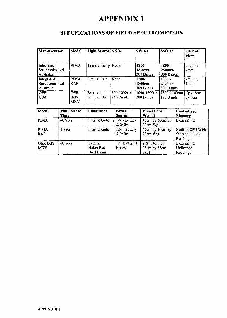
APPENDIX 1

SPECFICATIONS OF FIELD SPECTROMETERS

Manufacturer Model Light Source VNIR SWIRl SWIRl Field of View

Integrated PIMA Internal Lamp None 1200- 1800 - 2mmby Speetronies Ltd. 1800run 2500run 4mm Australia. 300 Bands 300 Bands Integrated PIMA Internal Lamp None 1200- 1800 - 2mmby Speetronies Ltd RAP 1800run 2500run 4mm Australia 300 Bands 300 Bands GER GER External 350-1000nm I 000-1800nm 1800-2500nm Upto 5em USA IRIS Lamp or Sun 216 Bands 200 Bands 175 Bands by 5em

MKV

Model Min. Record Calibration Power Dimensions/ Control and Time Source We!ght Memory

PIMA 60 Sees Internal Gold 12v - Battery 40em by 20em by External PC & 250v 20em 8kg

PIMA 8 Sees Internal Gold 12v - Battery 40em by 20em by Built In CPU With RAP & 250v 20em 6kg Storage For 200

Readings GERIRIS 60 Sees External 12v Battery 4 2 X (14em by External PC MKV Halon Pad Hours 25em by 25em Unlimited

Dual Beam 7kg) Readings

APPENDIX 1

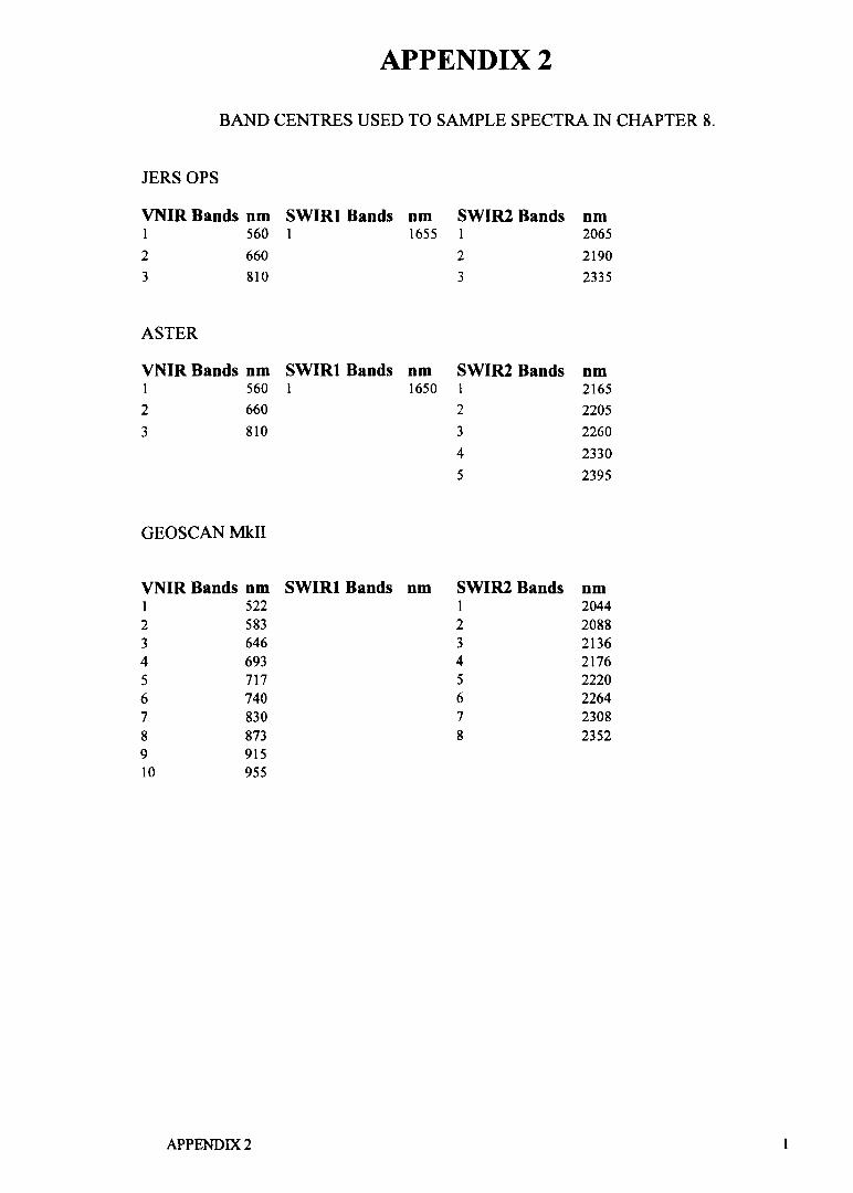
APPENDIX 2

BAND CENTRES USED TO SAMPLE SPECTRA IN CHAPTER 8.

JERS OPS

VNIR Bands nm SWIRl Bands nm SWIR2 Bands nm 1 560 1 1655 1 2065 2 660 2 2190 3 810 3 2335

ASTER

VNIR Bands nm SWIRl Bands nm SWIRl Bands nm 1 560 1 1650 1 2165 2 660 2 2205 3 810 3 2260

4 2330 5 2395

GEOSCAN MkII

VNIR Bands nm SWIRl Bands nm SWIRl Bands nm 1 522 1 2044 2 583 2 2088 3 646 3 2136 4 693 4 2176 5 717 5 2220 6 740 6 2264 7 830 7 2308 8 873 8 2352 9 915 10 955

APPENDIX 2

GERIS

VNIR Bands nm SWIRl Bands nm SWIR2 Bands nm 1 413 1 1260 I 2007.8

2 438 2 1380 2 2023.4

3 464 3 1500 3 2039.0

4 489 4 1620 4 2054.6

5 514 5 1740 5 2070.2

6 540 6 2085.8

7 565 7 2101.4

8 591 8 2117.0

9 616 9 2132.6

10 641 10 2148.2

11 667 11 2163.8

12 692 12 2179.4

13 718 13 2195.0

14 743 14 2210.6

15 768 15 2226.2

16 794 16 2241.8

17 819 17 2257.4

18 845 18 2273.0

19 870 19 2288.6

20 895 20 2304.2

21 921 21 2319.8

22 946 22 2335.4

23 972 23 2351.0

24 997 24 2366.6

25 1022 25 2382.2

26 1140 26 2397.8

27 2413.4

28 2429.0

29 2444.6

30 2460.2

31 2475.8

32 2491.4

APPENDIX 2 2

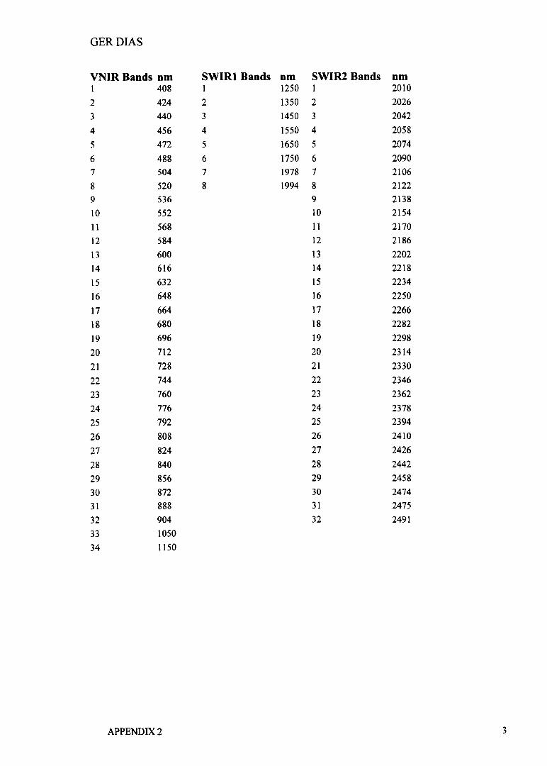
GERDIAS

VNIR Bands nm SWIRl Bands nm SWIR2 Bands nm 1 408 1 1250 1 2010

2 424 2 1350 2 2026 3 440 3 1450 3 2042

4 456 4 1550 4 2058

5 472 5 1650 5 2074 6 488 6 1750 6 2090 7 504 7 1978 7 2106 8 520 8 1994 8 2122 9 536 9 2138 10 552 10 2154 11 568 11 2170 12 584 12 2186 13 600 13 2202 14 616 14 2218

15 632 15 2234

16 648 16 2250

17 664 17 2266

18 680 18 2282

19 696 19 2298 20 712 20 2314

21 728 21 2330

22 744 22 2346

23 760 23 2362

24 776 24 2378 25 792 25 2394

26 808 26 2410

27 824 27 2426

28 840 28 2442 29 856 29 2458 30 872 30 2474 31 888 31 2475

32 904 32 2491

33 1050 34 1150

APPENDIX 2 3

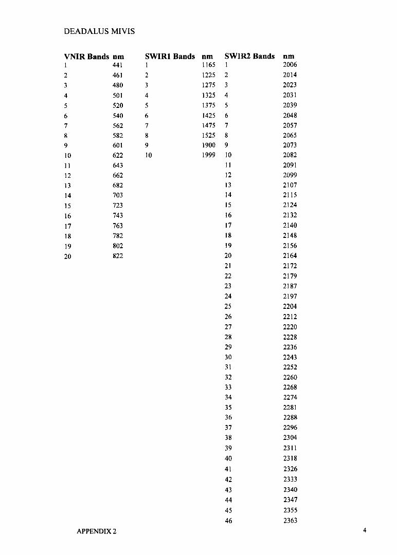
DEADALUS MIVIS

VNIR Bands nm SWIRl Bands nm SWIR2 Bands nm 1 441 1 1165 1 2006

2 461 2 1225 2 2014

3 480 3 1275 3 2023

4 501 4 1325 4 2031

5 520 5 1375 5 2039

6 540 6 1425 6 2048 7 562 7 1475 7 2057 8 582 8 1525 8 2065 9 601 9 1900 9 2073 10 622 10 1999 10 2082

11 643 11 2091 12 662 12 2099

13 682 13 2107

14 703 14 2115

15 723 15 2124

16 743 16 2132

17 763 17 2140

18 782 18 2148

19 802 19 2156

20 822 20 2164 21 2172 22 2179 23 2187 24 2197 25 2204 26 2212 27 2220 28 2228 29 2236 30 2243 31 2252 32 2260 33 2268 34 2274 35 2281 36 2288 37 2296 38 2304

39 2311 40 2318

41 2326

42 2333 43 2340 44 2347

45 2355

46 2363

APPENDIX 2 4

47 2370 48 2377 49 2384 50 2391 51 2398 52 2405 53 2412 54 2419 55 2426 56 2433 57 2440 58 2446 59 2453 60 2460 61 2467 62 2472

APPENDIX 2 5

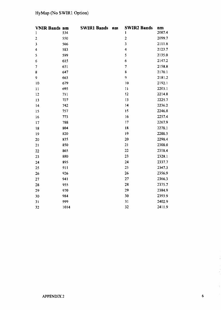
HyMap (No SWIRl Option)

VNIR Bands nm SWIRl Bands nm SWIR2 Bands nm I 534 1 2087.4

2 550 2 2099.7

3 566 3 2111.8

4 583 4 2123.7

5 599 5 2135.0

6 615 6 2147.2

7 631 7 2158.8

8 647 8 2170.1

9 663 9 2181.2

10 679 10 2192.1

11 695 11 2203.1

12 711 12 2214.8

13 727 13 2225.7

14 742 14 2236.2

15 757 15 2246.8

16 773 16 2257.4

17 788 17 2267.9

18 804 18 2278.1

19 820 19 2288.3

20 835 20 2298.4

21 850 21 2308.0

22 865 22 2318.4

23 880 23 2328.1

24 895 24 2337.7

25 911 25 2347.3

26 926 26 2356.9

27 941 27 2366.3

28 955 28 2375.7

29 970 29 2384.9

30 984 30 2393.9

31 999 31 2402.9

32 1014 32 2411.9

APPENDIX 2 6

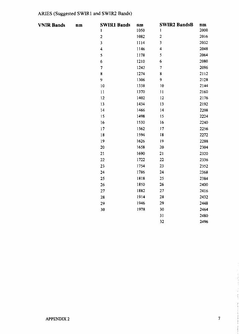
ARIES (Suggested SWIRl and SWIR2 Bands)

VNIRBands nm SWIRl Bands nm SWIRl BandsB nm 1 1050 1 2000

2 1082 2 2016

3 1114 3 2032

4 1146 4 2048

5 1178 5 2064

6 1210 6 2080

7 1242 7 2096

8 1274 8 2112 9 1306 9 2128 10 1338 10 2144 11 1370 11 2160 12 1402 12 2176 13 1434 13 2192 14 1466 14 2208 15 1498 15 2224 16 1530 16 2240

17 1562 17 2256 18 1594 18 2272 19 1626 19 2288 20 1658 20 2304 21 1690 21 2320 22 1722 22 2336

23 1754 23 2352 24 1786 24 2368 25 1818 25 2384 26 1850 26 2400

27 1882 27 2416

28 1914 28 2432

29 1946 29 2448

30 1978 30 2464 31 2480 32 2496

APPENDIX 2 7

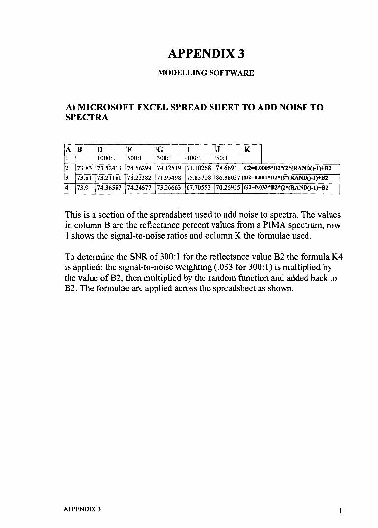
APPENDIX 3 MODELLING SOFTWARE

A) MICROSOFT EXCEL SPREAD SHEET TO ADD NOISE TO SPECTRA

A B D F G I J K 1 1000:1 500:1 300:1 100:1 50:1

2 73.83 73.524l3 74.56299 74.12519 71.10268 78.6691 C2=O.OO05*B2*(2 *(RANDo-l )+B2

3 73.81 73.21181 73.23382 71.95498 75.83708 86.88037 D2=O.OOl *B2*(2*(RANDO-l)+B2

4 73.9 74.36587 74.24677 73.26663 67.70553 70.26935 G2=O.033*B2*(2*(RANDO-l)+B2

This is a section of the spreadsheet used to add noise to spectra. The values in column B are the reflectance percent values from a PIMA spectrum, row 1 shows the signal-to-noise ratios and column K the formulae used.

To determine the SNR of300:1 for the reflectance value B2 the formula K4 is applied: the signal-to-noise weighting (.033 for 300:1) is multiplied by the value of B2, then mUltiplied by the random function and added back to B2. The formulae are applied across the spreadsheet as shown.

APPENDIX 3

B) C PROGRAM TO PRODUCE IMAGE DATA CUBES FROM SPECTRA

/********************************************************************* *****/ /* module specmodel */ /* this module is the main driver for the spectral modelling utility */ /********************************************************************* *****/

#include <stdio.h> #include <stdlib.h> #include "define.h" #include "specmodel.h"

void main(int argc, char *argv[])

char error flag = ERROR;

if (init(argc, argv) == OK) if (input() == OK)

if (readspec() == OK) if (writeimage() == OK)

error_flag = !ERROR;

terminate(error flag); exit (0) ; }

/*********************************************************************

*/ /* submodule init: */ /* this submodule opens the input and output files */ /********************************************************************* */

#include <stdio.h> #include <string.h> #include "define.h" #include "specmodel.h"

init(argc, argv) int argc; char *argv[]; {

/* Command line */ if (argc != NO_ARGUMENTS)

{

strcpy(message, "Usage: specmodel input_parameter_file output_image_file\n");

return (ERROR) ; }

strcpy(infile, argv[l]); strcpy(outfile, argv[2]);

/* open input parameter file */ if (! (infp = fopen (infile, "r")))

{

APPENDIX 3 2

sprintf(message, "Error in init: can't open %s", infile); return (ERROR) ; }

/* open output image file */ if (! (outfp = fopen (outfile, "w")))

{

sprintf(message, "Error in init: can't open %s", outfile); return (ERROR) ; }

return (OK) ; }

APPENDIX 3 3

/***********************************************************/

/* submodule input: */ /* this submodule reads the input parameter file */ /***********************************************************/

#include <stdio.h> #include <string.h> #include <stdlib. h> #include "define.h" #include "specmodel.h"

input () {

char text[80]; int i, bnd;

do

if (getline(infp, text, 3*BUFFERSIZE) <= 0) {

strcpy(message, "Error reading parameter file: noise percentage");

}

return (ERROR) ; }

while (text[O] == '#'); sscanf(text, "%f", &noise); if ( noise < 0 I I noise > 100

do

{

sprintf(message, "Invalid noise percentage: %f", noise); return (ERROR) ; }

if (getline(infp, text, 3*BUFFERSIZE) <= 0) {

strcpy(message, "Error reading parameter file: topographic range") ;

}

return(ERROR); }

while (text[O] == '#'); sscanf(text, "%f", &topo);

do

if (getline(infp, text, 3*BUFFERSIZE) <= 0) {

strcpy(message, "Error reading parameter file: x spectra") ;

}

return(ERROR); }

while (text[O] == '#'); sscanf(text, "%d", &xblocks); if ( xblocks < 0 I I xblocks > MAX X

{

sprintf(message, "Invalid no. x blocks: %d", xblocks); return(ERROR); }

APPENDIX 3 4

do

if (getline(infp, text, 3*BUFFERSIZE) <= 0) {

strcpy(message, "Error reading parameter file: y spectra") ;

}

return (ERROR) ; }

while (text[O] == '#'); sscanf(text, Hid", &yblocks); if ( yblocks < 0 I I yblocks > MAX Y

{

do

sprintf(message, "Invalid no. y blocks: %d", xblocks); return(ERROR); }

if (getline(infp, text, 3*BUFFERSIZE) <= 0) {

strcpy(message, "Error reading parameter file: no. pixels per block");

}

return (ERROR) ; }

while (text[O] == '#'); sscanf(text, Hid", &numpix);

do

if (getline(infp, text, 3*BUFFERSIZE) <= 0) { strcpy(message, "Error reading parameter file: bands"); return(ERROR); }

while (text[O] == '#'); sscanf(text, Hid", &bands); if ( bands < 0 I I bands > MAX_BANDS

{ sprintf(message, "Invalid no. bands: %d", bands); return(ERROR); }

for (i=O; i < bands; i++) {

do

if (getline(infp, text, 3*BUFFERSIZE) <= 0) {

strcpy(message, "Error reading parameter file: wavelengths");

}

return (ERROR) ; }

while (text[O] == '#'); sscanf(text, "%d%f", &bnd, &wav[i]); if (bnd < 0 I I bnd > MAX_BANDS)

return (OK) ;

APPENDIX 3

{

sprintf(message, "Invalid band number: %d", bnd); return (ERROR) ; }

5

/********************************************************** ************/ /* submodule getline: */ /* this submodule fetches a line from a text file. */ /********************************************************************* */

getline( fp, s, lim) */

/* get a line from file with file pointer fp

FILE *fp; char * S;

long lim; {

long c, i;

i = 0; while --lim> 0 && ( c

s [i++] c;

if ( c == LINE FEED s[i++] = LINEFEED;

sri] = '\0'; return(i); }

getc( fp ) != EOF && c != LINEFEED )

/***********************************************************/ /* submodule readspec: */ /* this submodule reads the files containing the spectra */ /***********************************************************/

#include <stdio.h> #include <string.h> #include <stdlib.h> #include "define.h" #include "specmodel.h"

readspec () {

char char int float

for (i=O; {

text[80]; buf[BUFFERSIZE]; i, j, k, x, y; w, r, w_old, r_old;

i < xblocks; i++)

for (j=O; j < yblocks; j++) {

/* Read x,y block numbers and spectra file name */ do

if (getline(infp, text, 3*BUFFERSIZE) <= 0) {

strcpy(message, "Error reading input parameter file: spectra file");

APPENDIX 3

return (ERROR) ; }

6

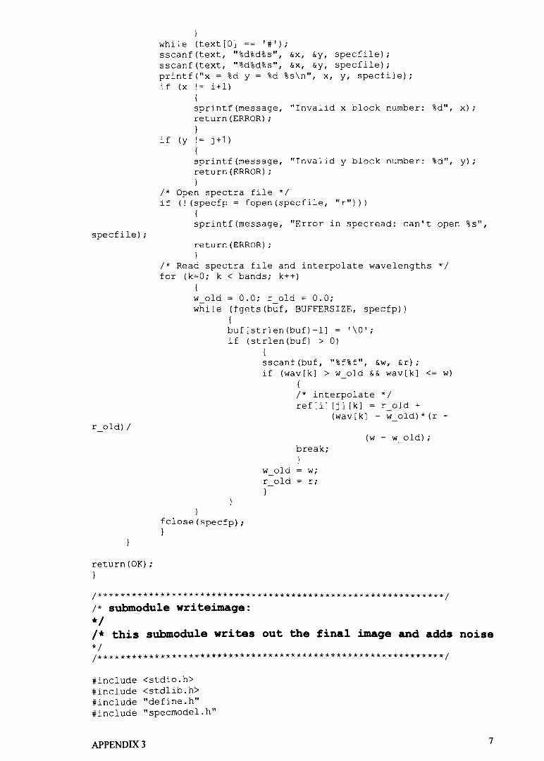
specfile);

return(OK); }

while (text[O] == 'I'); sscanf(text, "%d%d%s", &x, &y, specfile); sscanf(text, "%d%d%s", &x, &y, specfile); printf("x = %d Y = %d %s\n", x, y, specfile); if (x != i+l)

{

sprintf(message, "Invalid x block number: %d", x); return(ERROR); }

if (y != j+l) { sprintf(message, "Invalid y block number: %d", y); return(ERROR); }

/* Open spectra file */ if (! (specfp = fopen (specfile, "r")))

{

sprintf(message, "Error in specread: can't open Is",

return (ERROR) ; }

/* Read spectra file and interpolate wavelengths */ for (k=O; k < bands; k++)

{

wold 0.0; raId = 0.0; while (fgets(buf, BUFFERSIZE, specfp))

{

buf[strlen(buf)-l] = '\0'; if (strlen(buf) > 0)

fclose(specfp); }

{

sscanf(buf, "%f%f", &w, &r); if (wav[k] > w_old && wav[k] <= w)

{

/* interpolate */ ref[i] [j] [k] = r_old +

break; }

wold w; raId r; }

(wav[k] - w_old)*(r -

(w - wold);

/***************************************************** ********1

/* submodule writeimage: *1 1* this submodule writes out the final ~age and adds noise */ /*************************************************************/

#include <stdio.h> #include <stdlib.h> #include "define.h" #include "specmodel.h"

APPENDIX 3 7

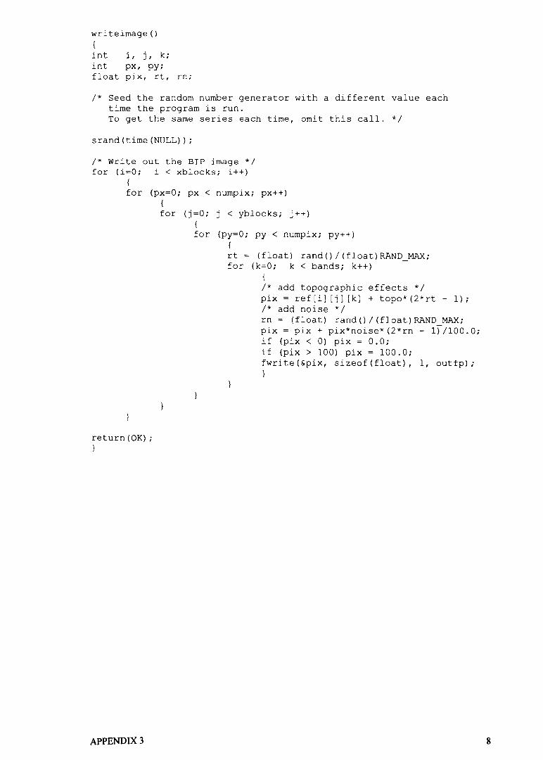
wri teimage () {

int i, j, k; int px, py; float pix, rt, rn;

/* Seed the random number generator with a different value each time the program is run. To get the same series each time, omit this call. */

srand(time(NULL)) ;

/* Write out the SIP image */ for (i=O; i < xblocks; i++)

{

for (px=O; px < numpix; px++) {

return(OK); }

APPENDIX 3

for (j=O; j < yblocks; j++) {

for (py=O; py < numpix; py++) {

rt = (float) rand()/(float)RAND_MAX; for (k=O; k < bands; k++)

{

/* add topographic effects */ pix = ref[i][j][k] + topo*(2*rt - 1); /* add noise */ rn = (float) rand()/(float)RAND_MAX; pix = pix + pix*noise*(2*rn - 1)/100.0; if (pix < 0) pix = 0.0; if (pix> 100) pix = 100.0; fwrite(&pix, sizeof(float), 1, outfp); }

8

/********************************************************************* **/ / * submodule terminate: *1 1* this submodule terminates the utility writing out the error message *1 /********************************************************************* **/

/* include table definitions */

#include <stdio.h> #include "define.h" #include "specmodel.h"

void terminate (error)

char {

error;

/* write error message to screen and exit if error */

printf("%s\n", message); if (error == ERROR)

exit(l);

fclose (infp) ; fclose(outfp) ;

APPENDIX 3 9

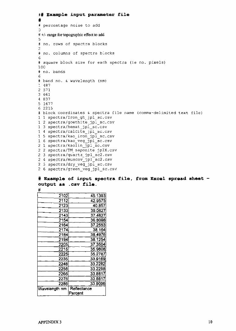
## Example input parameter file # # percentage noise to add o # +/- range for topographic effect to add 5 # no. rows of spectra blocks 2 # no. columns of spectra blocks 6 # square block size for each spectra (ie no. pixels) 100 # no. bands 6 # band no. & wavelength (nm) 1 487 2 571 3 661 4 837 5 1677 6 2215 # block coordinates & spectra file name (comma-delimited text file) 1 1 spectra/lron_gh_jpl_sc.csv 1 2 spectra/goethite_jpl_sc.csv 1 3 spectra/hemat_jpl_sc.csv 1 4 spectra/calclte_jpl sc.csv 1 5 spectra/kao iron jpl sc.csv 1 6 spectra/kao_veg_jpl_sc.csv 2 1 spectra/kaolin jpl sc.csv 2 2 spectra/TM_saponite jplX.csv 2 3 spectra/quartz_jpl_sc2.csv 2 4 spectra/muscov_jpl sc2.csv 2 5 spectra/dry_veg_jpl_sc.csv 2 6 spectra/green_veg_jpl sc.csv

# Example of input spectra file, from Excel spread sheet -output as .csv file. #

2102 45.1393 2112 42.9575 2123 40.857 2133 39.0627 2143 37.4627 2154 36.8098 2164 37.2553 2174 38.164 2184 38.4976 2194 38.1254 2205 37.3504 2215 35.9808 2225 35.2787 2235 33.9169 2246 33.2282 2256 33.2298 2266 33.8817 2276 33.8817 2286 33.9096

Wavelength nm Reflectance Percent

APPENDIX 3 10

APPENDIX 4

APPENDIX 4 GEOSCAN MklI CALIBRATION

1.0 INTRODUCTION

This appendix has been edited from a draft paper supplied by N Adronis the principal

engineer involved with the development of the GEOSCAN MklI scanner. It provides useful

background information on the system. The information in this document together with

data supplied by N Adronis was used by Dr A Becker to write a program (Page 18) to

convert ground spectral readings obtained with the GEOSCAN MkII scanner to

reflectance values. This results of using this program are discussed in Chapter 9 of the

thesis.

This paper describes the Spectral and Radiometric calibration procedures that can be used

on the GEOSCAN MkII Scanner.

The GEOSCAN MkII Scanner has been designed to discriminate reflectance and emittance

to the maximum sensitivity possible using the latest Scanner design techniques and

component technologies over three spectral regions. The measured sensitivity in the three

spectral bands are as follows:

Visible Spectrometer SWIR Spectrometer Thermal Spectrometer

Max of 0.25% reflectance Max of 0.4% reflectance Max of 0.05 degrees temperature

Typically reflectance can not be measured in a controlled environment of better than 1%.

Assuming only the AC component of a reflectance signal is recorded then a 8 bit digitising

system or 256 discrete levels is adequate. The high sensitivity has been achieved by using

large optics and the highest quality optical components.

The reflectance and temperature sensitivity degrades with the amount of induced

instrument noise and the ground illumination conditions. For example a visible channel

with a airborne signal to noise of 180:1 (Maximum 8 bit signal to noise ratio) will have a

reflectance sensitivity of approximately 1 %. As the energy illuminating the ground

decreases due to a low sun angle or poor atmospheric conditions the amount of instrument

induced noise will increase and degrade the instrument sensitivity.

APPENDIX 4

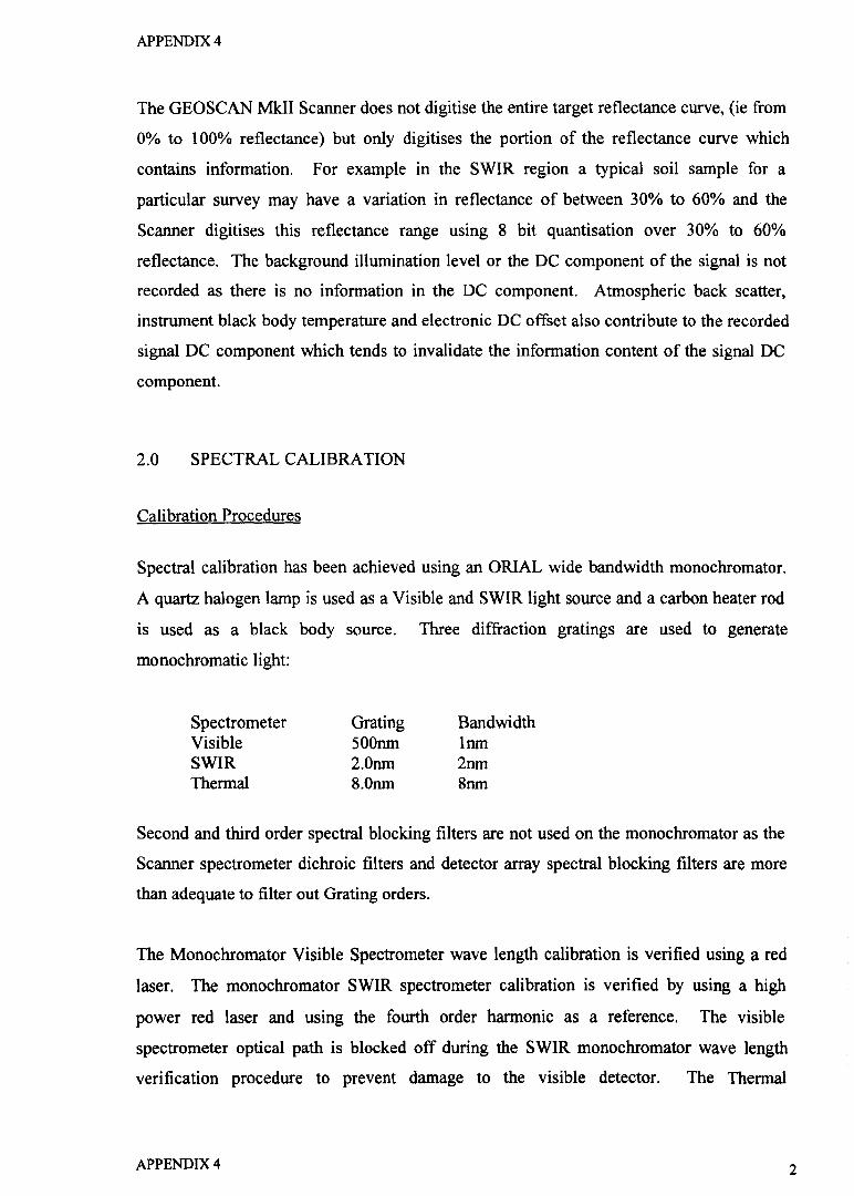
APPENDIX 4

The GEOSCAN MkII Scanner does not digitise the entire target reflectance curve, (ie from

0% to 100% reflectance) but only digitises the portion of the reflectance curve which

contains information. For example in the SWIR region a typical soil sample for a

particular survey may have a variation in reflectance of between 30% to 60% and the

Scanner digitises this reflectance range using 8 bit quantisation over 30% to 60%

reflectance. The background illumination level or the DC component of the signal is not

recorded as there is no information in the DC component. Atmospheric back scatter,

instrument black body temperature and electronic DC offset also contribute to the recorded

signal DC component which tends to invalidate the information content of the signal DC

component.

2.0 SPECTRAL CALIBRATION

Calibration Procedures

Spectral calibration has been achieved using an ORIAL wide bandwidth monochromator.

A quartz halogen lamp is used as a Visible and SWIR light source and a carbon heater rod

is used as a black body source. Three diffraction gratings are used to generate

monochromatic light:

Spectrometer Visible SWIR Thermal

Grating 500nm 2.0nm 8.0nm

Bandwidth Inm 2nm 8nm

Second and third order spectral blocking filters are not used on the monochromator as the

Scanner spectrometer dichroic filters and detector array spectral blocking filters are more

than adequate to filter out Grating orders.

The Monochromator Visible Spectrometer wave length calibration is verified using a red

laser. The monochromator SWIR spectrometer calibration is verified by using a high

power red laser and using the fourth order harmonic as a reference. The visible

spectrometer optical path is blocked off during the SWIR monochromator wave length

verification procedure to prevent damage to the visible detector. The Thermal

APPENDIX 4 2

APPENDIX 4

monochromator wave length calibration is verified by using the absorption lines of a

polystyrene plastic film.

A collimated monochromatic light source is injected into the telescope aperture using a

small off centred parabola. The scan mirror is rotated a 5Hz to minimise detector noise

and Scans across the aperture of the monochromator off centred parabola. The

monochromator is set to the zeroth order to provide a broad band light source and the

Scanning Telescope Pitch angle is adjusted to maximise the signal level. The

monochromator offset error is determined by adjusting and maximising the zeroth order

peak and the dial gauge zero setting. This offset is then applied to all monochromator

readings to generate an absolute wave lengths for the particular grating used.

The Scanner single channel CRO display is used to measure the intensity of the calibration

source. The CRO display calculated the maximum and minimum calibration peak values

and averaged 16 readings to remove the detector noise component. By sweeping the

monochromator wave length at 1 nanometre increments and recording the calibration peak

high and low values a band pass curve can be generated. These curves are normalised as

the signal value and the gain and offset settings between channels are not correlated.

Because there are no filters in the monochromator optical path and a high temperature

source is used then the energy generated by the monochromator over the narrow band pass

of a detector channel can be assumed to be linear. The Radiometric calibration results can

be used to generate a relative spectral response.

Visible Spectral Calibration

The Visible Spectral Calibration curves show that the position and shape of the band pass

curves are all different. The Visible detector is made up of a 35 element linear array and

by combining different detector elements channel a different band pass can be achieved.

Channel 1 is made up of two detector elements, channels 2 and 3 are made up of three

detector elements each, channels 4 to 6 are single adjacent detector elements and channels

7 to 10 are single detector elements with unused detector elements between the channels.

Channels 4 to 10 are gaussian in their spectral distribution which is due to the rectangular

detector elements imaging a rectangular field stop. Channels 2 and 3 should in theory have

a flat on the top as they are a addition of thee gaussian detector channels. Due to the non

linear frequency response of the dichroic filters used in the spectrometers to provide broad

APPENDIX 4 3

APPENDIX 4

band frequency splitting and diffraction grating multiple order filtering the tops of channels

2 and 3 band pass curves map the non linear response of these filters. Channel 1 has a

distorted band pass curve due to:

1. High attenuation of short wave lengths of Aluminium metal used in the front sufficed mirrors,

2. Poor response ofthe silicon detector at 400nm, 3. Square Visible camera lens aperture obstructing the short wave length.

SWIR Spectral calibration

The eight SWIR spectral response curves are mostly gaussian in distribution due to a

rectangular detector elements imaging a rectangular field stop. Channel 17 and 18 have

slightly distorted spectral response curves due to the non linear spectral response of the

dichroic filters used as broad band filter and grating multiple order filters.

Thermal Spectral Calibration

The six thermal spectral response curves are mostly gaussian in distribution due to a

rectangular detector elements imaging a rectangular field stop. Channel 20, 23 and 24

have a slightly distorted spectral response curves due to the non linear spectral response of

the dichroic filters used as broad band filter and grating multiple order filters. Channel 24

has a distorted gaussian shape and is due to the fall in optical efficiency at the longer wave

lengths.

3.0 RADIOMETRIC CALIBRATION

Warnings

To avoid missus of the Radiometric Calibration results, users of this information must note

the following:

APPENDIX 4 4

APPENDIX 4

1. The GEOSCAN MkII Scanner optical performance has changed significantly since February 1992 and there has been an improvement in the signal to noise performance of between 50% to 200% in the three spectrometers.

2. Radiometric Calibration Results are not valid for imagery flown before February 1992 due to the resurfaced mirrors and higher quality detectors.

3. The Radiometric Calibration coefficients will only convert the recorded digital data to power entering the Scanning telescope. Absolute ground radiometric power can not be determined due to the known atmospheric absorption between the aircraft and the ground. Use of telescope input power as a indication of ground illuminated and radiated power must be qualified.

4. The Radiometric Calibration coefficients will not be valid after 12 months due to the accumulated degradation in performance of seven mirror surfaces.

5. The calibration coefficients may be used to produce a relative spectral signature for channels of the same spectral signature for channels of the same spectrometers but can be used to generate a relative spectral response between the three spectrometers.

6. Due to the complex optical path of the Scanner built in calibration sources and the effect of the Scanner Telescope temperature the contribution of the calibration signal the recorded calibration source curves can only be used as a stable reference for scan runs of the same altitude and date.

7. Only the radiometric Gain coefficients in this report can be used for calibration and the user must generate separate offset, bias, Black body and Bias coefficient for different images.

Instrument Sensitivity Measurements

The GEOSCAN MkII Scanner has been designed to measure reflectance to better than

0.5% and with a temperature resolution of better than 0.1 degree.

Assuming a calibration lamp current is roughly proportional to irradiance, a 1 % change in

lamp current the GEOSCAN MIdI Scanner will detect a 4.5% change Visible spectrometer

signal level and a 3% change in the SWIR spectrometer signal level. This translates to the

Visible spectrometers sensitivity of better than 0.25% reflectance and a SWIR

spectrometer sensitivity of better than 0.3% reflectance.

APPENDIX 4 5

APPENDIX 4

Assuming the radiated power of a body of water is roughly proportional to temperature to

the power of four (ie Emissivity of water = 0.96) then for a 35 degree water temperature

with a 0.1 degree temperature change, the GEOSCAN MkII Scanner registers a 3% change

in signal level. This translates to a thermal spectrometer sensitivity of better than 0.05

degrees temperature.

The Spectrometer sensitivity degrades with the amount of detector induced random noise.

The spectrometer channel noise is proportional to the optical efficiency and a function of

wave length. The spectrometers efficiency has been designed to peak at the centre of

channels:

Visible Spectrometer: SWIR Spectrometer: Thermal Spectrometer:

Channel 4 Channel 13 Channel 21

The spectrometer channel sensitivity can be determined by using the channel signal to

noise figure for the recorded image. Most spectrometer channels have a signal to noise

value of 180: 1 to 100: 1 which is the maximum signal to noise figure for a 8 bit digitising

system.

From the signal to noise performance graphs it is apparent that the induced detector noise

is proportional to the Scanner mirror speed or ground resolution. As the Ground

integration time reduces the amount of induced noise increases. The Spectrometer noise

performance tests indicate that the visible detectors generate white noise across the entire

band pass. The SWIR detector noise power band width is roughly at the centre of the

Scanning bandwidth. The thermal detector noise power bandwidth is mostly low

frequency noise. The test flight airborne signal to noise figures indicate that most of the

visible channels have a signal to noise of 180: 1 and the SWIR and thermal channels have a

signal to noise of between 50:1 to 100:1. Because the visible channels have a signal to

noise of 180:1 which is the limit of the 8 bit digiti sing system the noise performance is

constant until the mirror speed exceeds 20Hz.

The GEOSCAN MkiI Scanner is designed to generate digital data that is proportional to

optical input power at the Scanner telescope. Linear equations can be used to convert the

recorded digital channel values to relative or absolute radiometric values.

APPENDIX 4 6

APPENDIX 4

Radiometric Calibration Procedures

Visible and SWIR radiometric calibration has been achieved using a standard calibrated

lamp mounted 150mm from the centre of a white body target. A teflon based target is used

as a white body source with a 96% to 99% reflectance efficiency. The Target is mounted

at 45 degrees to the vertical axis of the Scanner telescope to position the calibration lamp

outside the Scanner field of view. All the calibration source component spectral responses

have been modelled to enable the telescope input power to be calculated for the 18 visible

and SWIR channels. Two calibration peaks are generated by covering up 50% of the

calibration target with a black body source. Different gain and offset settings are used to

image the two calibration peaks which are used to calibrate the system gain and offset

coefficients.

Thermal radiometric calibration is achieved by using two heated bodies of water at

different temperatures. Knowing the emissivity of water and the black body equation the

power at the six thermal wave lengths can be calculated. The two bodies of water are

located at +/- 30 degrees from the telescope vertical axis.

Calibration Lamp Irradiance Calibration

The ORIEL calibration lamp No.9 _ 056 has been supplied with a list of course irradiance

values from 400nm to 2500nm. The irradiance data can not be used to derive the black

body equation due to the non back body lamp curve. Since we are not imaging the top of

the black body curve and are effectively using the linear parts of both sides of the black

body cure, we can use linear interpolation to calculate the irradiance at the 18 Visible and

SWIR channels.

White Body Target Reflectance Calibration

The White body target used to generate a full aperture spherical light source is a

SPECTRALON SR T -99-180 teflon based target. This target is supplied with coarse

reflection data from 250nm to 2500nm and has a reflectance efficiency of between 95.5%

to 99.3%. Since irradiance power can only be calculated to within 2%, linear interpolation

is adequate to calculate the reflectance efficiency for the 18 Visible and SWIR channels.

APPENDIX 4 7

APPENDIX 4

The Calibration target reflectance efficiency spread sheet located in appendix A has been

set up to calculate the reflectance for the 18 Visible and SWIR channels and the channel

wave lengths have been linked back to the spectral response curves.

Calibration Target Illumination Distribution

The calibration lamp irradiance values have been measured 50mm from the lamp and since

the calibration lamp is 150mm from the target the energy reflected off the target is

approximately 10% of the published irradiance values. The calibration target is mounted

45 degrees to the telescope axis and the oval telescope foot print can be mapped on the

calibration target using a 150mm and 20mm scanning mirror shape. Using the inverse

square law the average target attenuation can be calculated by dividing the oval foot print

into a 10mm grid and averaging the lamp attenuation at grid points. The Illumination

distribution graph illustrates the illumination profiled of the Visible and SWIR calibration

light source. The calculated average target attenuation has been linked to the Radiometric

calibration spread sheets.

Thermal Source Black Body Calibration

Two heated water bodies are used as black body sources to calibrate the thermal

spectrometer. Planck's formula for a black body can be used to determine the radiated

power for the six thermal channels:

M(l) ClIl **5*{exp{c211 *T)-I)

Where:

M{l)

CI C2 1 T

=

= = = =

Black Body radiated power in Watts per square meter per wavelength 3.74 E-16 Watts per square meter 1.44E-2 Meters per degrees Kelvin Wave length in meters Absolute temperature in degrees Kelvin

Spectral Emissivity can be calculated as follows:

APPENDIX 4 8

APPENDIX 4

eel) =

Where:

E(l) =

M(1 material)/(M(1 black body))

Spectral Emissivity of a material Radiated power of material M(l material) =

M(1 Black body)= Radiated power of a black body source as given in the above equation.

The emissivity of water is as follows:

Distilled Water Smooth ice Frost Crystals Snow

=

=

0.96 at 20 degrees C 0.06 at -10 degrees C 0.98 at -10 degrees C at -10 degrees C

The equation for the radiated power of a body of water can be derived from the above

equation:

M(1) 0.96*Cl/1 **5*(ex(c2/1 *T)-l)

Using this formula the radiated power for the six thermal channels can be determined using

the water temperature.

Gain Calibration

The Scanner uses an eight bit digital gain system to amplify the spectrometer signal before

digitising. The digital gain circuit has been wired up with an approximate exponential gain

setting response and is required to handle the large dynamic range of detector signals

generated. From the Gain calibration results and the Scanner digital gain circuit we can

derive and verify the gain setting equation as being y=l/(l-x).

Offset Calibration

The Scanner uses an eight bit digital offset system to remove the DC components or the

background illumination components from the detector signals to allow maximum digitised

APPENDIX 4 9

APPENDIX 4

signal information content. From the Offset calibration results the offset setting response

curve is linear.

Raw Image Data Radiometric Conversion

There are several problems in converting the spectrometer recorded digital value to an

absolute power:

1. Calibration lamps with a calibration target can only be calibrated to within 2% reflectance. The Visible and SWIR spectrometers have a sensitivity of better than 0.5% reflectance.

2. Thermal calibration sources can only be held stable to within 0.1 degrees. The Thermal spectrometer has a sensitivity of better than 0.1 degrees.

3. The atmospheric absorption between the aircraft and the ground IS

unknown.

4. The Atmospheric absorption between the ground and the sun is unknown.

5. Atmospheric back scatter effects of the image illumination invalidate radiometric ground control points in the shorter wave lengths.

Until these problems are solved an airborne Scanner that measures absolute spectra can not

be built. The value of absolute radiometric calibrated imagery has not yet been

demonstrated.

Visible Radiometric Calibration

From the visible spectrometer optical, analog and digital circuits we can determine the

relationship between the visible spectrometer spectral channel digital pixel value and the

telescope input power:

Byte=((Signal+Bias-O*(255-0ffset))/G/(255-Gain)

or

Signal=(Byte*G*(255-Gain)) - Bias + 0*(255-0ffset)

APPENDIX 4 10

APPENDIX 4

Where:

Signal

Byte G =

Gain =

Bias = o Offset =

Telescope input power for the channel wave length in Micro Watts per square centimetre per nanometre wave length. Eight bit unsigned digit pixel value Optical and electronic gain coefficient Eight bit unsigned digital gain value Trans impedance amplifier offset error bias Electronic offset gain coefficient Eight bit unsigned digital offset value

Due to the high trans impedance amplifier impedance of greater than 1 Mega ohm any

input offset error in the first stage of amplification in the spectrometer preamplifier is

amplified and included in the detector signal. Unfortunately the bias voltage varied with

amplifier temperature and since the Visible spectrometer is effectively in the aircraft

airflow this value will vary according to the aircraft altitude. The bias voltage contributes

about 5% to the total signal DC component.

Using a black body target as a zero reference and a white body source as a 100% and 50%

calibration lamp source the value of the G, 0 and Bias coefficients can be calculated as

follows:

G = (signall-signaI2)/(byte l-byte2)/(255-Gain)

For a signal level of zero and two different gain and offset readings:

Bias = (Byte2*G*(255-Gain2) * (255-0ffsetl)

o =

-Byte 1 *G*(255-Gainl) * (255-0ffset2» /(Offset2-offset 1) (Signal-Byte*G*(255-Gain)+Bias)/(255-0ffset)

Because the radiometric tests were performed immediately after power-up there was a

small amount of drift in the bias voltage during testing as the amplifiers heated up and

resulted in a large variation in the offset coefficient for various gain and offset settings. A

more accurate offset coefficient can be derived using gain and offset setting with larger

than a 5% difference.

From these test results we can use the gam coefficient to calibrate visible data for

amplitude for images flown after February 1992. Since the electronic gain is fixed to

within 2% components tolerance and the optical gain is fixed by the efficiency of the

optical components then the gain coefficient will be valid for at least 12 months. Optical

components efficiency tends to degrade rapidly in the shorter wave lengths.

APPENDIX 4 11

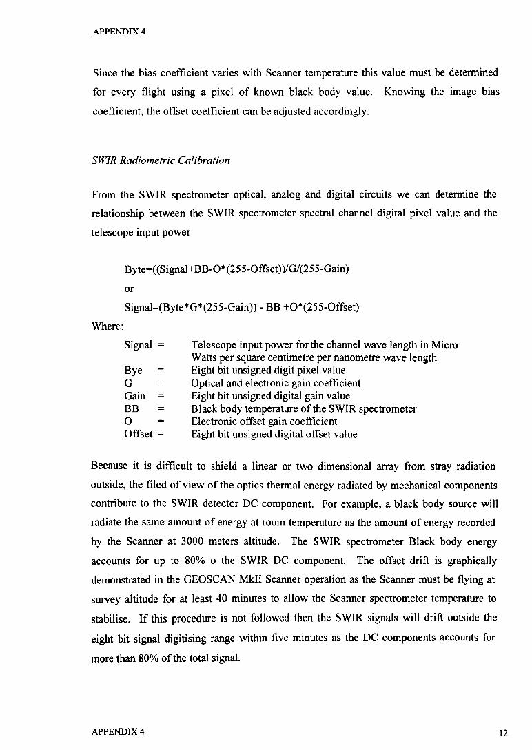
APPENDIX 4

Since the bias coefficient varies with Scanner temperature this value must be determined

for every flight using a pixel of known black body value. Knowing the image bias

coefficient, the offset coefficient can be adjusted accordingly.

SWIR Radiometric Calibration

From the SWIR spectrometer optical, analog and digital circuits we can determine the

relationship between the SWIR spectrometer spectral channel digital pixel value and the

telescope input power:

Where:

Byte=((Signal+BB-O*(255-0ffset))/G/(255-Gain)

or

Signal=(Byte*G*(255-Gain)) - BB +O*(255-0ffset)

Signal =

Bye = G = Gain = BB 0 =

Offset =

Telescope input power for the channel wave length in Micro Watts per square centimetre per nanometre wave length Eight bit unsigned digit pixel value Optical and electronic gain coefficient Eight bit unsigned digital gain value Black body temperature ofthe SWIR spectrometer Electronic offset gain coefficient Eight bit unsigned digital offset value

Because it is difficult to shield a linear or two dimensional array from stray radiation

outside, the filed of view of the optics thermal energy radiated by mechanical components

contribute to the SWIR detector DC component. For example, a black body source will

radiate the same amount of energy at room temperature as the amount of energy recorded

by the Scanner at 3000 meters altitude. The SWIR spectrometer Black body energy

accounts for up to 80% 0 the SWIR DC component. The offset drift is graphically

demonstrated in the GEOSCAN MklI Scanner operation as the Scanner must be flying at

survey altitude for at least 40 minutes to allow the Scanner spectrometer temperature to

stabilise. If this procedure is not followed then the SWIR signals will drift outside the

eight bit signal digiti sing range within five minutes as the DC components accounts for

more than 80% of the total signal.

APPENDIX 4 12

APPENDIX 4

Using a black body target as a zero reference and a white body source as a 100% and 50%

calibration lamp source the value of the G, 0 and Bias coefficients can be calculated as

follows:

G = (signall-signaI2)/(bytel-byte2)/(255-Gain)

For a signal level of zero and two different gain and offset readings:

BB = (Byte2*G*(255-Gain-Gain2) * (255-0ffsetl) -Byte 1 *G*(255-Gainl) * (255-0ffset2» /( offset2-offset 1)

0= (Signal-Byte*G*(255-Gain)+Bias)/(255-0ffset)

From the SWIR spectrometer Radiometric Calibration spread sheet you will note that the

gain coefficient is within 5% for the different radiometric readings.

The offset and black body coefficients were not calculated as these results are only valid

for the Scanner at room temperature.

From these test results we can use the gam coefficient to calibrate SWIR data for

amplitude for images flown after February 1992. Since the electronic gain is fixed to

within 2% components tolerance and the optical gain is fixed by the efficiency of the

optical components, then the gain coefficient will be valid for at least 18 months. Optical

efficiency degrades slowly for SWIR wave length.

Since the BB coefficient varies with Scanner temperature this value must be determined

for every flight using a pixel of known black body value. Knowing the image bias

coefficient the offset coefficient can be adjusted accordingly.

Thermal Radiometric Calibration

From the SWIR spectrometer optical, analog and digital circuits we can determine the

relationship between the Thermal spectrometer spectral channel digital pixel value and the

telescope input power:

Byte=( (Signal-DC=Bias-O* (25 5-0ffset) )/G/(25 5-Gain)

APPENDIX 4 13

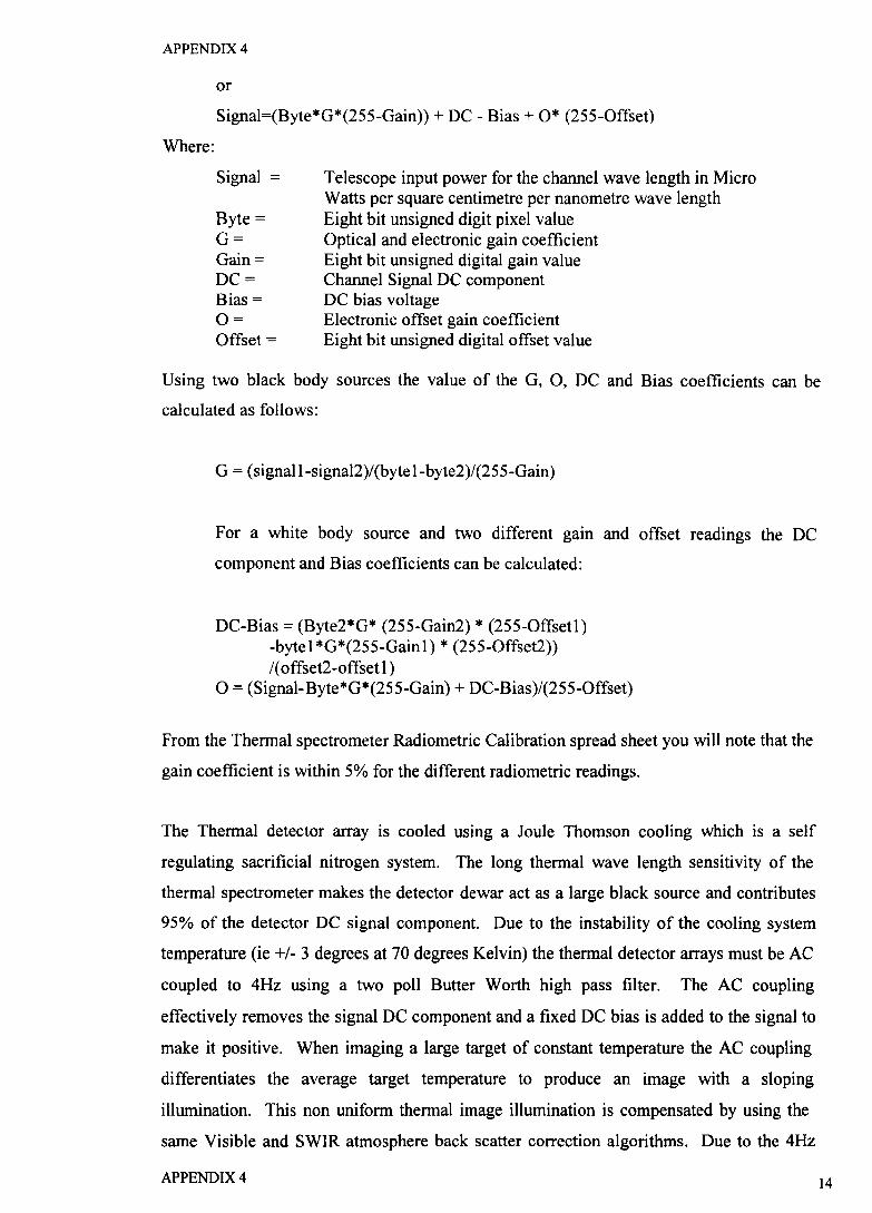
APPENDIX 4

or

Signal=(Byte*G*(255-Gain» + DC - Bias + 0* (255-0ffset)

Where:

Signal =

Byte = G= Gain = DC= Bias = 0= Offset =

Telescope input power for the channel wave length in Micro Watts per square centimetre per nanometre wave length Eight bit unsigned digit pixel value Optical and electronic gain coefficient Eight bit unsigned digital gain value Channel Signal DC component DC bias voltage Electronic offset gain coefficient Eight bit unsigned digital offset value

Using two black body sources the value of the G, 0, DC and Bias coefficients can be

calculated as follows:

G = (signall-signaI2)/(byte l-byte2)/(255-Gain)

For a white body source and two different gam and offset readings the DC

component and Bias coefficients can be calculated:

DC-Bias = (Byte2*G* (255-Gain2) * (255-0ffsetl) -by tel *G*(255-Gainl) * (255-0ffset2» I( offset2-offset I)

0= (Signal-Byte*G*(255-Gain) + DC-Bias)/(255-0ffset)

From the Thermal spectrometer Radiometric Calibration spread sheet you will note that the

gain coefficient is within 5% for the different radiometric readings.

The Thermal detector array is cooled using a louIe Thomson cooling which is a self

regulating sacrificial nitrogen system. The long thermal wave length sensitivity of the

thermal spectrometer makes the detector dewar act as a large black source and contributes

95% of the detector DC signal component. Due to the instability of the cooling system

temperature (ie +/- 3 degrees at 70 degrees Kelvin) the thermal detector arrays must be AC

coupled to 4Hz using a two poll Butter Worth high pass filter. The AC coupling

effectively removes the signal DC component and a fixed DC bias is added to the signal to

make it positive. When imaging a large target of constant temperature the AC coupling

differentiates the average target temperature to produce an image with a sloping

illumination. This non uniform thermal image illumination is compensated by using the

same Visible and SWIR atmosphere back scatter correction algorithms. Due to the 4Hz

APPENDIX 4 14

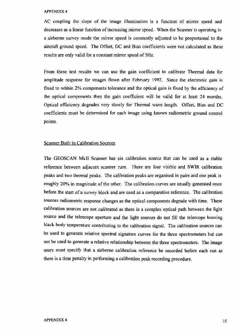
APPENDIX 4

AC coupling the slope of the image illumination is a function of mirror speed and

decreases as a linear function of increasing mirror speed. When the Scanner is operating in

a airborne survey mode the mirror speed is constantly adjusted to be proportional to the

aircraft ground speed. The Offset, DC and Bias coefficients were not calculated as these

results are only valid for a constant mirror speed of 5Hz.

From these test results we can use the gain coefficient to calibrate Thermal data for

amplitude response for images flown after February 1992. Since the electronic gain is

fixed to within 2% components tolerance and the optical gain is fixed by the efficiency of

the optical components then the gain coefficient will be valid for at least 24 months.

Optical efficiency degrades very slowly for Thermal wave length. Offset, Bias and DC

coefficients must be determined for each image using known radiometric ground control

points.

Scanner Built in Calibration Sources

The GEOSCAN MkII Scanner has six calibration source that can be used as a stable

reference between adjacent scanner runs. There are four visible and SWIR calibration

peaks and two thermal peaks. The calibration peaks are organised in pairs and one peak is

roughly 20% in magnitude of the other. The calibration curves are usually generated once

before the start of a survey block and are used as a comparative reference. The calibration

sources radiometric response changes as the optical components degrade with time. These

calibration sources are not calibrated as there is a complex optical path between the light

source and the telescope aperture and the light sources do not fill the telescope housing

black body temperature contributing to the calibration signal. The calibration sources can

be used to generate relative spectral signature curves for the three spectrometers but can

not be used to generate a relative relationship between the three spectrometers. The image

users must specify that a airborne calibration reference be recorded before each run as

there is a time penalty in performing a calibration peak recording procedure.

APPENDIX 4 15

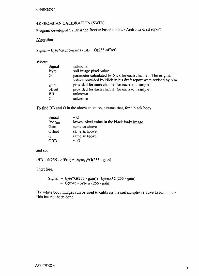
APPENDIX 4

4.0 GEOSCAN CALlBRA nON (SWIR)

Program developed by Dr Anne Becker based on Nick Andronis draft report.

Algorithm

Signal = byte*G(255-gain) - BB + 0(255-offset)

Where: Signal Byte G

gain offset BB o

unknown soil image pixel value parameter calculated by Nick for each channel. The original values provided by Nick in his draft report were revised by him provided for each channel for each soil sample provided for each channel for each soil sample unknown unknown

To find BB and 0 in the above equation, assume that, for a black body:

and so,

Signal ByteaB Gain Offset G OBB

=0 lowest pixel value in the black body image same as above same as above same as above =0

-BB + 0(255 - offset) = -bytesB*G(255 - gain)

Therefore,

Signal = byte*G(255 - gain)) - bytesB*G(255 - gain) = G(byte - bytesB)(255 - gain)

The white body images can be used to calibrate the soil samples relative to each other. This has not been done.

APPENDIX 4 16

APPENDIX 4

Program Code

lIS System 600 code to implement the calibration procedure algorithm described on the previous page:

1* Calibration Geoscan MkII data. Designed to work on soil sample padded with a black body image section on the left and a white body image section on the right.

Calibration parameters are read from a data file which lists, one per line, for each channel, the G parameter which remains fixed and the gain values which are changed for each samples. The parameter file also lists the sizes of the data image and the black body image so that the correct sections can be read in.

#include <stdio.h> #include <stdlib.h>

#include "xanth/source/ind/inc/standard. h" #include "xanth/source/ind/inc/ errordef. h" #include "iio/source/ind/inC/imdef. h"

#define numchannels 8

CPUgeocalibrate (Ichan, Iname, Icount, Ochan, Oname, Ocount, prmfile, outfile) int Ichan[], Icount, Ochan[], Ocount; String Iname[], Oname[], prmfile, outfile; {

int dtype, isx, isy, isz, isw; int bufsize, channel, npix, n; int image, line; int BBss, BBns, BBsl, BBnl, IMss, IMns, IMsl, IMnl; char strbuf[100], prmstr[25]; char calfile[100], uncalfile[100]; double G[10], gain[10]; double sum, BB, 1M; double bw[20); Byte *buf, *p; float callM; float *realbuf, *realp; FILE *prmfp; FILE *calfp, *uncalfp;

r Set bandwidth values */ bw[1) = 0.044; bw[2) = 0.048; bw[3) = 0.046; bw[4) = 0.044; bw[5) = 0.044; bw[6] = 0.044; bw[7] = 0.046; bw[8] = 0.042;

r Allocate buffer space */ bufsize = 50000; but = (Byte *) cMEMget(bufsize*4); realbut = (float *) cMEMget{butsize*4);

r Open the input image */ IMopen{lchan, AZ(lname[O]), 0, &dtype, &isx, &isy, &isz, &isw);

APPENDIX 4 17

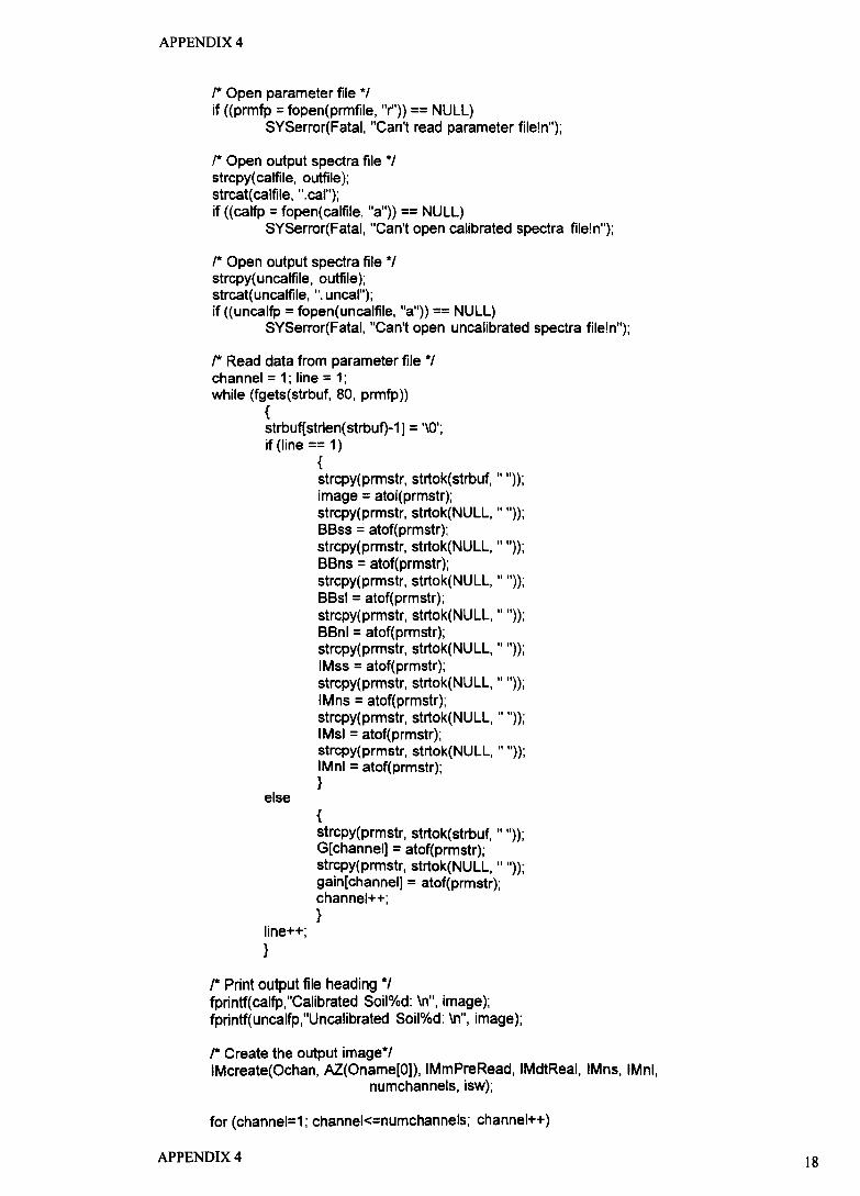
APPENDIX 4

1* Open parameter file */ if ({prmfp = fopen{prmfile, lOr"~»~ == NULL)

SYSerror{Fatal, "Can't read parameter file!n");

1* Open output spectra file */ strcpy{ calfile, outfile); strcat{calfile, ".cal"); if ({calfp = fopen{calfile, "a"» == NULL)

SYSerror(Fatal, "Can't open calibrated spectra file!n");

1* Open output spectra file */ strcpy(uncalfile, outfile); strcat(uncalfile, ". uncal"); if «uncalfp = fopen(uncalfile, "a"» == NULL)

SYSerror(Fatal, "Can't open uncalibrated spectra file!n");

/* Read data from parameter file */ channel = 1; line = 1; while (fgets(strbuf, 80, prmfp»

{ strbuf[strlen(strbuf}-1] = '\0'; if (line == 1)

else

line++; }

{ strcpy(prmstr, strtok(strbuf, " "»; image = atoi(prmstr); strcpy(prmstr, strtok(NULL, " "»; BBss = atof(prmstr); strcpy(prmstr, strtok(NULL, " "»; BBns = atof(prmstr); strcpy(prmstr, strtok(NULL, " "»; BBsl = atof(prmstr); strcpy(prmstr, strtok(NULL, " "»; BBnl = atof(prmstr); strcpy(prmstr, strtok(NULL, " "»; IMss = atof(prmstr); strcpy(prmstr, strtok(NULL, " "»; IMns = atof(prmstr); strcpy(prmstr, strtok(NULL, " "»; IMsl = atof(prmstr); strcpy(prmstr, strtok(NULL, " "»; IMnl = atof(prmstr); }

{ strcpy(prmstr, strtok(strbuf, " "»; G[channel] = atof{prmstr); strcpy(prmstr, strtok(NULL, " "»; gain[channel] = atof(prmstr); channel++; }

/* Print output file heading */ fprintf(calfp,"Calibrated Soil%d: \n", image); fprintf(uncalfp,"Uncalibrated Soil%d: \n", image);

1* Create the output image*/ IMcreate(Ochan, AZ(Oname(O)), IMmPreRead, IMdtReal, IMns, IMnl,

numchannels, isw);

for (channel=1; channel<=numchannels; channel++)

APPENDIX 4 18

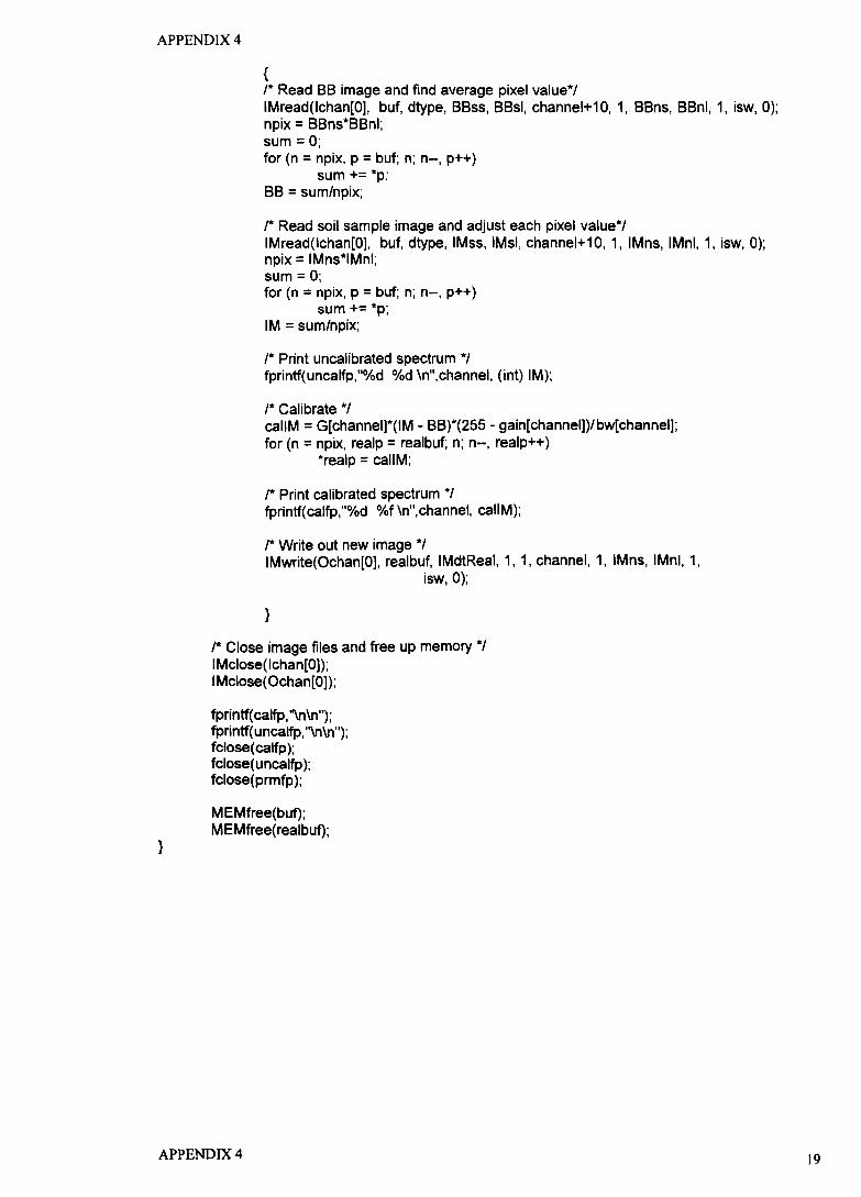
APPENDIX 4

}

{ 1* Read BB image and find average pixel value*/ IMread(lchan[O], buf, dtype, BBss, BBsl, channel+10, 1, BBns, BBnl, 1, isw, 0); npix = BBns*BBnl; sum = 0; for (n = npix, p = buf; n; n--, p++)

sum += *p; BB = sum/npix;

/* Read soil sample image and adjust each pixel value*/ IMread(lchan[O), buf, dtype, IMss, IMsl, channel+10, 1, IMns, IMnl, 1, isw, 0); npix = IMns*IMnl; sum = 0; for (n = npix, p = buf; n; n--, p++)

sum += *p; 1M = sum/npix;

/* Print uncalibrated spectrum */ fprintf(uncalfp,"%d %d \n",channel, (int) 1M);

/* Calibrate *1 caliM = G[channel)*(IM - BB)*(255 - gain[channel))/bw[channel); for (n = npix, realp = realbuf; n; n--, realp++)

*realp = callM;

1* Print calibrated spectrum */ fprintf(calfp,"%d %f \n",channel, caIlM);

1* Write out new image */ IMwrite(Ochan[O], realbuf, IMdtReal, 1, 1, channel, 1, IMns, IMnl, 1,

isw, 0);

}

1* Close image files and free up memory */ IMclose(lchan[O)); IMclose(Ochan[O));

fprintf( calfp, "\n\n"); fprintf( uncalfp,''\n\n''); fclose( calfp ); fclose( uncalfp); fclose(prmfp );

M EMfree(buf); MEMfree(realbuf);

APPENDIX 4 19