Surface and volume rendering techniques to display 3-D data

Surface and Volume Rendering Techniques to Display 3D Data : An Overview of Basic

Principles Christian Barillot, Ph.D.

INSERM U-335,

Neurosurgery Dept., Pontchaillou Hospital, 35033 Rennes Cedex, France

ph: (+33) 99 33 68 65, FAX: (+33) 99 28 41 03, email: [email protected]

ABSTRACT

This paper gives an overview of 3D display techniques for medical data including surface and

volume rendering techniques. A special emphasis is done on the most recent methodology

which becomes widely used to render medical volumetric data sets: Ray-Tracing which makes

possible the volume rendering of voxel data. This paper describes the basic fundamentals of the

fuzzy display algorithms involved in the volume rendering techniques. The different techniques

presented in this paper will take example from applications using 3D display of CT, MRI or

DSR data and mapping of functional and anatomical data by means of 3D textures. Finally this

paper concludes by giving some perspectives of 3D display of volume and surface data.

Keywords: 3D Display, Volume Rendering, Ray-Tracing, Medical Imaging

1. INTRODUCTION

1.1 Overview of 3D Display Methods

Almost all physical processes have now been used to image human anatomy from X-ray

computed tomography (CT), angiography, and positron emission tomography (PET) to

magnetic resonance imaging (MRI). These medical imaging modalities have introduced

significant changes in routine patient care, adding diagnostic evidence and expanding

therapeutic efficiency. Nevertheless, the mechanisms of medical image understanding are

complex. They rely particularly upon the knowledge of organ topologies and the relations they

share. In other respects, the multiplicity of pathological processes may induce many structural

and functional outlines. The morphology, functional data, and the different stigma of a lesional

state are as many elements to integrate in the space. The image presentation modes, based on

scan sections or radiographic views, do not completely meet the requirements of diagnostic

interpretation, therapeutic decision, or surgical operation. They require the physician to do

sequential examinations of images and mental 3D reconstruction.

During the last fifteen years, these reasons have supported all the attempts developed

toward 3D viewing, matching closely advances in medical imaging, computer technology, and

computer graphics research. This area conforms with the constant concern for better viewing for

better understanding and better understanding for better medicine.

At the present time, two main different ways to display 3D medical data can be defined.

The first one can be called Surface Rendering and the second one Volume rendering.

TriangulationSegmentation

Segmentation

Graph Search

Set of Polygons

Octree

Binary Sequence

Source Data

InterpolationGrey Level

Volume

Binary Volume

Segmentation and Region

Growing

Recursive Subdivision

Direct Projection

(ray tracing)

Set of Voxel Faces

Set of Voxels

Polygon Oriented Display

Voxel Oriented Display

Volumetric Display

Surface RenderingVolume Rendering

Figure 1: Overview of Surface and Volume Rendering Methods.

1.2 Surface Rendering Methods.

Within this family, the earliest method was the polygon oriented method, it appeared

along the arrival of triangulation algorithms using planar contours [1][2]. These methods have

been mostly applied to the 3D representation of anatomical structures from parallel slices [3],

example is shown on plate a.

A classical approach consists firstly from the binary sequence of the source data to extract

a set of contours representing the surface. The tiling of this surface is done by joining the

different points belonging to the contours with triangles in order to optimize a criterion (volume,

area of triangles, length of segments, ...) within a planar graph. This method gives a surface data

base formed by polygons which can be displayed with standard computer graphics display

algorithms. Boissonnat [4] has proposed another method which is based on the Delaunay

triangulation and the tessellation of planar contours. As others, this new approach carries out a

solution to the difficult problem of the 3D connectivity of a set of contours [5] [3].

Using a polygonal approach to represent surfaces, some works have also been done to

display 3D structures apart from parallel slices data set such as display of vascular systems from

angiograms [6].

Later, some surface rendering techniques with a voxel oriented approach were developed

[7-10]. These new techniques have improved the accuracy and the reliability of the 3D

representations. For these methods, either binary or grey scale volumes can be used. With both

volumes the data must be interpolated from the original sequence in order to obtain an

homogeneous matrix of voxel along the three main axes. Within the volume (binary or not), a

surface tracking algorithm is executed to extract the surface components (voxels or faces of

voxels) in order to build up a surface database. More recently, Lorensen et al. [11] have

proposed a method called "marching cube" which performs a surface tracking in order to

construct a polygonal data base (with triangles) based on the surface voxel neighborhood

topology. For all of these methods, the surface display is done by rotating the surface elements

(voxels, faces of voxels, triangles) along the viewpoint and projecting them on the screen.

Several rendering can be performed on these data bases like depth or depth-gradient shading (as

described later on). When surfaces are extracted from binary volumes, the surface normal

vectors are estimated according to the topology of the surface voxels. Nevertheless the best

rendering quality is obtained by using 3D grey level gradients to estimate the surface normal

vectors which can then be used by the diffuse and/or specular lighting models [9] [12].

1.3 Volume Rendering Methods.

Volume display techniques have appeared more recently and have the ability to display

either surfaces with shading or part of the volume with its grey level values or both together

[13-19]. The main feature of these techniques is to display data directly from the grey scale

volume. The selection of the data which will appear on the screen is done during the projection

of the voxels as a function of different attributes such as grey level or gradient values (for

surface segmentation), spatial coordinate (for volume cutting), volume set operation (union,

intersection, difference of volume) or transparency for instance. The two most representative

methods "Ray Tracing" and "Octree Encoding" are further described in this paper with a special

emphasis to the ray-tracing approach which tend to be the de facto standard for volume data

representation in medicine.

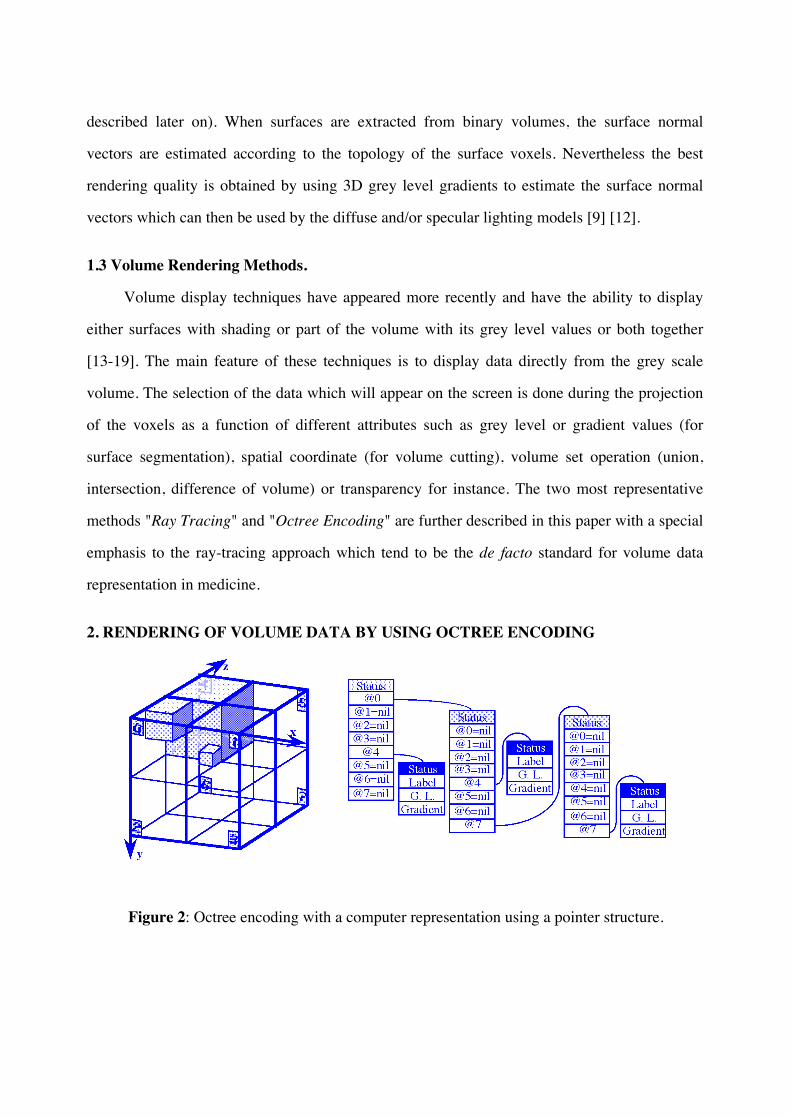
2. RENDERING OF VOLUME DATA BY USING OCTREE ENCODING

Figure 2: Octree encoding with a computer representation using a pointer structure.

One of the first attempts to the representation of volume data and the search of a

hierarchical structure has used the octree encoding [20] [13]. The octree coding which is part of

the family of the kD-trees is obtained by a recursive subdivision of the 3D space into eight sub-

volumes (octants) in order to generate a tree wherein a node contains all the information about

the corresponding enclosed cubical volume (figure 2). Every operation on the volume data will

be performed upon this tree.

Coding

Several octree representations have been proposed, they can differ either by their types of

subdivision or by their computer representations. This computer representation can be made by

means of pointers. In a pointer representation, a number of fields are associated with tree nodes,

eight of them specifying the pointers on the children (figure 2) [21] [22]. This technique is an

easy way to store intensity values in terminal nodes as well as surface normal vectors for a

better rendering of the objects. Nevertheless, the computation of surface normal vectors would

be very time consuming on the octree itself (search of neighborhood over the nodes to compute

the gradient) so it is usually performed only once during the octree construction process. Since

pointers structures can be very memory consuming, solutions without pointers have been

proposed. Coded trees [23] [24] are made by a list of all tree nodes arranged according to a

given tree traversal mode. Linear octrees [25] take only into account full nodes, each node is

represented by a code called "location key" allowing its localization within the tree.

Display and Manipulation

The visualization of octree data bases can be performed in two ways. One is based on the

object rotation and its projection along one of the octree orthogonal planes, some efficient

rotation algorithms have been proposed to solve this problem [13] [26]. A second approach

keeps the object at the same position and moves the observer. Only visible nodes are then

projected upon the image plane, which can be described by a quadtree. In this case overlapping

techniques have been developed [13]. For a direct projection, the computation of the vertices

corresponding to the three visible faces of a voxel are performed and these faces are filled.

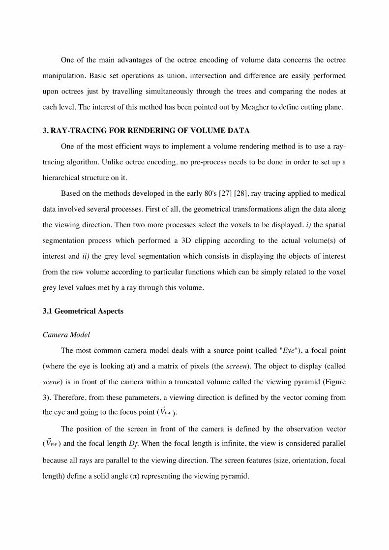
One of the main advantages of the octree encoding of volume data concerns the octree

manipulation. Basic set operations as union, intersection and difference are easily performed

upon octrees just by travelling simultaneously through the trees and comparing the nodes at

each level. The interest of this method has been pointed out by Meagher to define cutting plane.

3. RAY-TRACING FOR RENDERING OF VOLUME DATA

One of the most efficient ways to implement a volume rendering method is to use a ray-

tracing algorithm. Unlike octree encoding, no pre-process needs to be done in order to set up a

hierarchical structure on it.

Based on the methods developed in the early 80's [27] [28], ray-tracing applied to medical

data involved several processes. First of all, the geometrical transformations align the data along

the viewing direction. Then two more processes select the voxels to be displayed, i) the spatial

segmentation process which performed a 3D clipping according to the actual volume(s) of

interest and ii) the grey level segmentation which consists in displaying the objects of interest

from the raw volume according to particular functions which can be simply related to the voxel

grey level values met by a ray through this volume.

3.1 Geometrical Aspects

Camera Model

The most common camera model deals with a source point (called "Eye"), a focal point

(where the eye is looking at) and a matrix of pixels (the screen). The object to display (called

scene) is in front of the camera within a truncated volume called the viewing pyramid (Figure

3). Therefore, from these parameters, a viewing direction is defined by the vector coming from

the eye and going to the focus point ( ! V vw ).

The position of the screen in front of the camera is defined by the observation vector

( ! V vw ) and the focal length Df. When the focal length is infinite, the view is considered parallel

because all rays are parallel to the viewing direction. The screen features (size, orientation, focal

length) define a solid angle (π) representing the viewing pyramid.

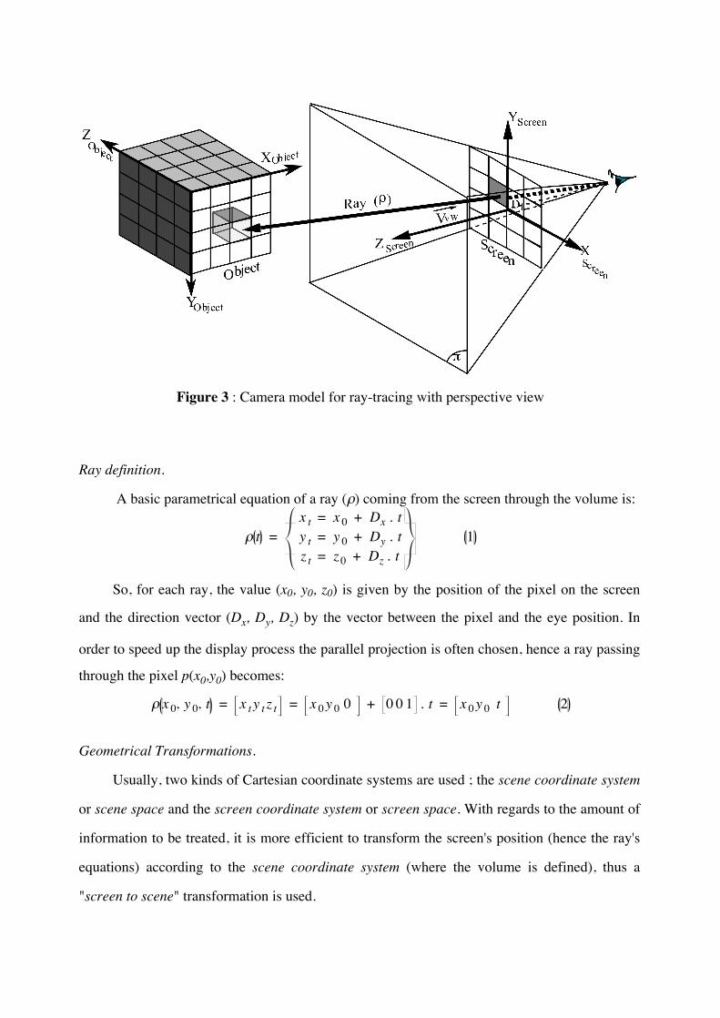
Figure 3 : Camera model for ray-tracing with perspective view

Ray definition.

A basic parametrical equation of a ray (ρ) coming from the screen through the volume is:

ρ t =x t = x 0 + Dx . ty t = y 0 + Dy . tz t = z0 + Dz . t

1

So, for each ray, the value (x0, y0, z0) is given by the position of the pixel on the screen

and the direction vector (Dx, Dy, Dz) by the vector between the pixel and the eye position. In

order to speed up the display process the parallel projection is often chosen, hence a ray passing

through the pixel p(x0,y0) becomes:

ρ x 0, y 0, t = x t y t z t = x 0y 0 0 + 0 0 1 . t = x 0y 0 t 2

Geometrical Transformations.

Usually, two kinds of Cartesian coordinate systems are used ; the scene coordinate system

or scene space and the screen coordinate system or screen space. With regards to the amount of

information to be treated, it is more efficient to transform the screen's position (hence the ray's

equations) according to the scene coordinate system (where the volume is defined), thus a

"screen to scene" transformation is used.

Therefore, after transformation, the equation of a ray becomes: ρ x 0, y 0, t = x t

, y t, z t, = x 0y 0 t • R + T 3

where

R = [rij]i,j∈[1,3] is the 3x3 rotation matrix.

T = [Tx Ty Tz] is the translation vector.

In order to simplify this equation, a point on the ray can be evaluated as a function of the

point before it, on this ray ; the chain coding of the ray can then be expressed at the instant ti as :

ρ x 0, y 0, ti - ρ x 0, y 0, ti-1 =

x t i, - x t i-1

, = ti - ti-1 • r31

y t i, - y t i-1

, = ti - ti-1 • r32

z t i, - z t i-1

, = ti - ti-1 • r33

4

So, now we can have the general equation of the ray at the instant ti within the scene

coordinate system :

ρ x 0, y 0, t =ρ x 0, y 0, t0 = x 0

, y 0, z0, = x 0y 0 0 • R + T

ρ x 0, y 0, ti = ρ x 0, y 0, ti-1 + r31r32r33 • Δt5

where (Δt = ti - ti-1 ) is the ray sample.

Look-up tables can be used to implement these equations [29].

3.2 Spatial Segmentation

Volume of Interest Definition

This stage consists in defining a volume of interest (VOI) wherein the rays have to be

computed. The projection on the screen of this VOI will define the effective pixels about which

the rays have to be cast in order to speed up the display process. A very common way to

perform this task is to define a bounding box which surrounds the VOI. The size of this box is

usually set to the dimensions of the volumetric data set.

Another way to define the volume of interest is to set up a polygonal structure to bound

this volume [18] [29]. A particular advantage of this method is its ability to define a more

complicated shape of the VOI. Hence, during the ray casting process, this polygonal structure is

projected first on the screen in order to set up the 3D clipping region and to measure the actual

length of each ray by means of a Z-buffer. Another advantage of this approach is its ability to

define cutting planes within the volumetric data set. Indeed, when a polygon or part of it clips

the volume, a pixel related to this image region can easily be assigned by the grey level value of

the first voxel met by a ray. This feature figures out a convenient tool to perform a "digital

dissection" of the volume. Because of the use of a Z-buffer, this technique makes also possible

the fusion of polygonal objects with volume data just by using polygon projection and shading

algorithms along with the ray tracer.

Other techniques can be used to define the VOI like for instance binary octrees which are

effective tools for a geometrical modelling of binary object shapes as explained before. Voxel

surfaces description, as described in §1.2, can also be used to set up a well fitted initialization of

the VOI for the ray tracer.

Multiple Object Display

Another task for the spatial segmentation concerns the display of multiple objects from the

same volume as shown in the ANALYZE™ software package developed by the Mayo Clinic

[18] [29] [30]. After a labelling process performed before the display stage, an object map can

be used in order to define at which object a voxel belongs to. By attaching parameters to this

object map, colors and/or opacities can be assigned to each voxel of the VOI and then be used in

the rendering process. In a similar way, 3D textures can be assigned to a VOI or to an object

map in order to overlap parametrical information to the original volume. Use of this feature can

be found in application fields where fusion of multimodal or multiparametric data is of high

interest (i.e. radio oncology, nuclear medicine, neuronal imaging as EEG or MEG, …) (plate d).

3.3 Grey Level Segmentation and Rendering Aspects.

This stage consists in displaying particular objects from the volume of interest selected

previously. One function is assigned to each pixel of the screen, this function is often related to

the voxel grey level values met by a ray throughout the volume. One of the most spectacular

properties of this process is its ability to display a new object (i.e. a new surface) as easily and

rapidly as to change the viewpoint. Several approaches can be used to render the grey level

values. Regarding the rendering aspects these techniques can be classified into two families i)

transmission oriented display methods and ii) reflection oriented display methods. Concerning

this second family, two grey level segmentation approaches can be chosen: the binary

segmentation which comes out with the display of iso-intensity surfaces (IIS) and the fuzzy

segmentation which allows the display of fuzzy objects with their grey level continuities.

3.3.1 Transmission oriented display.

These methods do not involved any surface identification process. A ray goes totally

through the VOI and the pixel value is computed as an integrated function. Two different

display methods are usually proposed: the brightest pixel display where the pixel value is the

brightest grey level value along the ray (method often used to display angiograms from MRI)

and the weighted summation display where the pixel value is a weighted average of the voxel

grey level values recorded along the ray [29] .

3.3.2 Rendering of Iso-Intensity Surfaces

Different approaches can be used for the rendering of iso-intensity surfaces. The most

common segmentation process is to classify the object of interest by using a binary function of

the voxel grey level values (e.g. a plain threshold) which makes the selection of the inner- and

the outer-object. Thus as a ray goes through the volume, the binary segmentation function

returns a true value when this ray meets the first voxel with a grey level value above the

threshold. Three main ways of rendering can then be applied [29]:

• Depth shading : A pixel value is only related to the depth of the first voxel along the ray

which belongs to the actual IIS of the volume of interest.

• Depth gradient shading : This rendering is just an enhancement of the previous method.

A pseudo gradient is computed upon the screen's depth values (Z-buffer) to approximate the

surface orientation which can be used by some well-known lighting models (i.e. Gouraud or

Phong's models) [31].

• Gradient shading : This rendering technique consists in estimating the surface orientation

on each voxel detected on the IIS by computing the gradient vector related to these voxel

neighborhoods [9] [12]. From this surface normal estimation the same diffuse and/or specular

lighting models are used.

3.3.3. Active Fuzzy Segmentation

Principle

This new approach specifically applied to a volume representation method consists in

assuming that the display of an object cannot be simplified as a binary grey level intensity

function (e.g. an IIS). An alternative is to use a so called fuzzy function for which within a range

of grey level values the object surface is not present, for another range the surface is partially

present and for a third range the surface is totally present. This merging of information is called

volumetric compositing and is an approximation of the visibility calculations required to render

a semi-transparent gel [32] [33]. The implementation of this method consists firstly in assigning

classification coefficients (α) to each voxel along the ray. The classification can be pre-

computed [34] [35] or processed during the rendering pipeline as described below. Then the

classification coefficients and the radiosities computed on each voxel are merged together

during the compositing process.

Volumetric Compositing Process

The approach introduced by Porter and Duff [32] and developed in medical imaging by

Drebin and Levoy [34] [35] presents the classification coefficients as opacity values which can

be used by a transparency compositing model. Assuming that a classification coefficient

behaves as an opacity value and represents the probability for a voxel to belong to the structure

of interest, the volumetric compositing is just an extension of the well known transparency

model:

B’ = F • α + (1-α) • B

where F and B are the foreground and the background colors and α the opacity value of F.

Porter has extended this model to set up a general compositing formula between two

medium A and B:

c = a • µA + b • µB

where (a = A • αA), (b = B • αB), (c = C • αC) are the composite colors of the media A, B

and C

µA , µB are the compositing functions for (resp.) the media A and B getting values in {0,

1, αA, 1-αA, αB , 1-αB}

αA, αB, αC are the opacity coefficients of media A, B and C with αC = αA + (1-αA) • αB

Concerning the compositing process of volume data, Drebin et al. have proposed to used

the over relation from the set of functions defined by Porter. These formulations can be related

to the more general Fuzzy Set mathematical theory where the classification coefficients

represent the grade of memberships of fuzzy sets A, B, C and where the compositing formula

are algebraic operations on fuzzy sets as presented by Zadeh [36]. From these concepts, the

compositing of volume data can be defined as follows :

• Let Z be the number of voxels met by the ray ρ within the volume V.

• Let (Iz, αz) be the couple color-opacity assigned to the voxel vz along ρ, (z < Z ). The

color Iz is the luminescence computed at vz, the opacity αz (e.g. the grade of

membership of vz to the ray ρ) is computed in the classification process. The composite

color I’z is the following algebraic product : I’z = Iz · αz

FTB

(C0, α' 0)

(I0 , α0 )

(C3, α' 3)(C2, α' 2)

(C1, α' 1)

(C4, α' 4)

(I2 , α2 )(I3 , α3 )

(I1 , α1 )

BTF

(ρ)

Figure 4 : Example of compositing with four voxels along the ray (Z = 4).

• Let Cz and Cz+1 be the compositing colors computed at (resp.) the anterior and the

posterior border of vz and (α’z, α’z+1) their relative compositing opacities (see figure 4),

the corresponding composite colors are : C’z = Cz · α’z and C’z+1 = Cz+1 · α’z+1

The volumetric compositing of Z voxels along a ray ρ, starting at (x0, y0) can be computed

from the back to the front as :

Cz,= Iz

,over Cz+1

,

α z,= α z + 1 − α z α z+1

, ⇔Cz,= Iz , C z+1

,; α z

α z,= α z⊕ α z+1

,

where C = (Α, Β ; λ) = Αλ + (1−λ) Β is the convex combination of A and B by the fuzzy value λ

as defined by Kaufmann [37].

γ = α ⊕ β = α + β − α β = 1 − ( 1 − α ) ( 1 − β ) is the algebraic sum of fuzzy values α and β.

The equivalent iterative equation is: Cz,= Czα z

,= Izα z + 1 − α z C z+1α z+1

,

Hence, the integration of voxels vz (z < Z )) along ρ(x0, y0) from the back to the front is :

ρBTFx0,y0; Z =C0,

α 0,; C 0

,=

Z

∑z=0

Izα z •

z-1

Πζ=0

1-αζ with : α 0,=

Z

⊕z=0

α z = 1 −Z

Πz=0

1-α z ; α Z,= α Z

According to the same conditions, the volumetric compositing can be computed from the

front to the back of ρ:

Cz+1,= C z

,over Iz

,

α z+1,

= α z,+ 1 − α z

,α z

⇔

Cz+1,= C z , Iz

,; α z

,

α z+1,

= α z,⊕ α z ⇔

Cz+1,= Cz+1α z+1

,= Czα z

,+ 1 − α z

,Izα z

Thus, the integration of voxels vz (z < Z )) along ρ(x0, y0)) from the front to the back is:

ρFTBx0,y0; Z =CZ,

α Z,; C Z

,=

Z-1

∑z=0

Izα z •

z-1

Πζ=0

1-αζ

with :

α Z,=

Z-1

⊕z=0

α z = 1 −Z-1

Πz=0

1-α z ; α 0,= 0

The equality condition between the two compositing formula is :

ρBTF = ρFTB ⇔ ∃ vz , z < Z ; α z = 1

Classification Process

The major problem concerning the fuzzy rendering is to select a relevant classification

function which makes the display as good, fast and reliable as possible. One way to find out this

classification function is to perform a fuzzy segmentation process and to assign the result to a

fuzzy object map used by the ray tracer [38-40]. Otherwise and more generally, the fuzzy set

theory gives suggestions about classical fuzzy membership functions which can be used to

display 3D volumes [37]. The main classification functions AGL are based on the voxel grey

level intensities and can be divided into two families called edge and step with three different

shapes (linear, gaussian and sinus) (figure 5). Actually the classification function the most

commonly used is the linear step function. The edge functions are more relevant to display low

intensity structures hidden by data with higher grey level values or iso-intensity structures as

isodoses in oncology for instance. Usually, the final classification coefficient αv assigned to a

voxel v is the algebraic product of three different fuzzy values:

αv = αGL • α∇ • αMAX

where αGL is the classification coefficient of voxel v according to its grey level, it can also

be called grade of membership of v in the fuzzy set AGL.

α∇ is the classification coefficient of v according to its gradient intensity, it can also be

called grade of membership of v in the fuzzy set A∇.

αMAX is the maximum classification value of voxel v representing the maximum opacity

of the structure of interest.

Several structures of interest (SOI) may have to be displayed during the volumetric

compositing process, the resulting classification coefficient αv assigned to the voxel v according

to the membership coefficients αvs of the SOI s (s ∈ [0, S]) is:

α v=S

⊕s=0

α sv

Therefore, by using this formula several structures may be merged together within the

same rendering process according to their own membership functions.

0

0,1

0,2

0,3

0,4

0,5

0,6

0,7

0,8

0,9

1

lineargaussiansinus

xmaxxmin x0

w w

α step linear x =

0 : x ≤ x minx - x minx max-x min

: x min< x < x max

1 : x ≥ x max

α step gaussianx =

0 : x ≤ x min

e-x - x max

2

2w2 : x min< x < x max1 : x ≥ x max

α step sinusx =

0 : x ≤ x min12+ 12sin

π

2•x - x 0w

: x min< x < x max

1 : x ≥ x max

0

0,1

0,2

0,3

0,4

0,5

0,6

0,7

0,8

0,9

1

lineargaussiansinus

xmaxxmin x0

w w

wfwf

α edge sinusx =

0 : x ≤ x min , x ≥ x max

12+ 12sin

π

w-wf• x - x 0 +

w+wf2

: x min< x < x 0- wf

1 : x 0 - wf ≤ x ≤ x 0+ wf

12- 12sin

π

w-wf• x - x 0 -

w+wf2

: x 0+ wf < x <x max

0 : x ≤ x min , x ≥ x maxx - x minw-wf

: x min< x < x 0- wf

1 : x 0 - wf ≤ x ≤ x 0+ wfx max - xw-wf

: x 0+ wf < x <x max

α edge linear x =

0 : x ≤ x min

e-x - x 0

2

2 w2

2

: x min< x < x max

0 : x ≥ x max

α edge gaussianx =

Figure 5: Fuzzy membership functions used for voxel classification

4. DISCUSSION AND CONCLUSION

Most research efforts in 3D medical imaging have been directed toward designing

efficient display methods. This rapid overview of 3D rendering techniques of medical data

shows up that encouraging results have been provided during the last fifteen years. This short

survey is well completed by recent literatures which emphasize the variety of approaches [3]

[42-44]. This experience underlines that no unique way can cover the entire domain of 3D

imaging in medicine. Indeed, even though volume rendering and especially ray-tracing can be

considered as the most sophisticated and general method to display 3D medical data, surface

rendering still remains the most relevant technique for displaying non commensurate

information like anatomical atlases for instance (see plate a). Hence, one of the main issue is to

select the most appropriate rendering method according to the data acquisition modes and the

medical relevance.

The future of 3D medical imaging depends on our ability to handle and to improve the

overall stages involved in the patient management. This includes the image acquisition, the

communication and the archiving of data (pointer to the PACS systems), the processing and the

fusion of multi-sensors information as well as the development of dedicated applications.

So beyond the actual use of 3D rendering tools which mainly remains in the field of

"looking at the data” (i.e. radiological applications). The challenge of tomorrow will aim in

extending the practical use of these techniques in other application fields (i.e radio oncology,

neurology, neurosurgery, plastic and reconstructive surgery...). Three dimensional rendering

techniques are going to improve by using the outcomes of many research efforts like in PACS

for communication and archiving aspects, in data fusion for the merging of multi-sensors

information (multimodality fusion, merging of anatomical and functional data) or in non rigid

data fusion for the warping of graphical representation of a priori knowledges (i.e anatomical

atlases) with in vivo data. Finally, the clinical acceptance of 3D rendering application will be

widely improved through the availability of well defined user interfaces. In this way, the efforts

carried out by the Mayo Clinic in developing the ANALYZE™ software package bring an

important piece to the edification of comprehensive and effective multi-dimensional medical

imaging systems.

6. ACKNOWLEDGEMENTS

The author expresses appreciation to their colleagues in the U335 INSERM unit in Rennes

and in the Biodynamic Research Unit at Mayo Clinic, Rochester MN, for their valuable

contributions to my research activity. Special recognition is given to Pr J.M. Scarabin and Dr B.

Gibaud for their early vision in three dimensional medical imaging, this special recognition goes

also to Pr R.A. Robb and A. Larson for their support regarding my research on ray-tracing. Data

bases were provided by Pr J. Talairach, Mayo Clinic and GE-CGR.

7. REFERENCES

1. Keppel E : Approximating Complex Surfaces by Triangulation of Contours Lines. IBM J Res Develop 19, pp.2-11, (1975)

2. Fuchs H, Kedem ZM, Uselton SP : Optimal Surface Reconstruction from Planar Contours. Comm of the ACM, Vol.20, pp.693-702, (1977)

3. Barillot C, Gibaud B et al. : Computer Graphics in Medicine: A Survey. CRC Critical Reviews in Biom Eng, Vol.15(4), pp.269-307, (1988)

4. Boissonnat, JD : Shape reconstruction from planar cross-sections. Computer Vis Graphics & Image Proc vol. 44(1) , pp.1-29, (1988)

5. Menhardt W, Carlsen IC : An Interactive environment for shaded perspective displays of MR tomograms, Special Issue on Computer Graphics, J.M. Scarabin, J.L. Coatrieux Eds, Innov Technol Biol Med, vol. 8(1) pp.104-120, (1987)

6. Barillot C, Gibaud B, Scarabin JM, Coatrieux JL: Three-Dimensional Reconstruction of Cerebral Blood Vessels. IEEE Computer Graphics & Applications, Vol.5(12), pp.13-19, (1985)

7. Herman GT, Liu H : 3-D Display of Human Organs from Computed Tomograms. Comp. Graph & Im Proc, Vol.9(1), pp.1-21 (1979)

8. Artzy E, Frieder G, Herman GT : The Theory, Design, Implementation and Evaluation of a Three-Dimensional Surface Detection Algorithm. Comp Graph & Im Pro., Vol.15, pp.1-24, (1981)

9. Barillot C, Gibaud B, Luo LM, Scarabin JM : 3-D Representation of Anatomic Structures from CT Examinations. Proc SPIE Biostereometrics'85, Vol.302, pp.307-314, (1985 b)

10. Heffernan PB., Robb RA : A New Method for Shaded Surface Display of Biological and Medical Images. IEEE Transactions on Medical Imaging, Vol.MI-4, pp.26-38,(1985)

11. Lorensen WE, Cline HE “Marching Cube: A High Resolution 3D Surface Construction Algorithm.” Computer Graphics, Vol. 21, N°3, Jul.1987, pp.163-169, (1987)

12. Höhne KH, Bernstein R : Shading 3D Images from CT Using Grey-Level Gradients. IEEE Trans on Medical Imaging, Vol.5(1), pp.45-47,(1986)

13. Meagher D : Geometric Modeling Using Octree Encoding. Comp Graph & Im Proc, Vol.19(2), 129-147, (1982)

14. Schlusselberg DS, Smith WK, Woodward DJ : Three-Dimensional Display of Medical Image Volumes. Proc. of 7th NCGA, Vol.III, pp.114-123, Anaheim 1986

15. Höhne KH, Riemer M, Tiede U : Viewing Operation for 3-D Tomographic Grey Level Data. Proc CAR'87, pp.599-609, Springer-Verlag Ed., (1987)

16. Trousset Y, Schmitt F : Active Ray-Tracing for 3D Medical Imaging. In: Proc Eurographics'87, pp.139-149, Amsterdam, 1987

17. Herman GT : Three-dimensional imaging on a CT or MR scanner. J Computer Assist Tomogr, Vol.12, pp.450-458 (1988)

18. Robb RA, Barillot C : Interactive Display and Analysis of 3-D Medical Images. IEEE Trans on Medical Imaging, Vol.8(3), pp.217-226, (1989)

19. Chen HH, Huang TS : A survey of construction and manipulation of octrees. Comput Vis Graph Image Proc, Vol.43, pp.409-431, (1988)

20. Jackins C, Tanimoto SL : Oct-trees and their use in presenting three dimensional objects, Comput Graph Image Proc, Vol.14, pp.249-270, (1980)

21. Meagher D : The manipulation analysis and display of 3D medical objects using octree encoding techniques, Special Issue on Computer Graphics, J.M. Scarabin, J.L. Coatrieux Eds, Innov Technol Biol Med, Vol.8(1), pp.23-36, (1987)

22. Jannin P, Gibaud B, Barillot C, Scarabin JM, Bouliou A : Octree encoding with volume and surface information in medical imaging. In: Proc. 9th IEEE EMBS Conference, Boston 1987

23. Cohen Y, Landy MS, Pavel M : Hierarchical coding of binary images. IEEE Trans Pat Anal Mach Intel, Vol.7(3) pp.284-298, (1985)

24. Sandor J : Octree data structures and perspectives imagery, Computer and Graphics, Vol.9(4) pp.393-405, (1985)

25. Gargantini I : Linear octrees for fast processing of three dimensional objects, Comput Graph Image Proc, Vol.20 pp.356-374, (1982)

26. Weng J, Ahuja N : Octree representation of objects in arbitrary motion, representation efficiency. Comp Graph & Im Proc, Vol.39, pp.167-182, (1987)

27. Roth SD : Ray Casting for Solid Modeling. Computer Graphics and Image Processing, Vol. 18(2), pp.109-144, (1982)

28. Kajiya JT : Ray Tracing. Tutorial Notes, ACM SIGGRAPH'83, (1983)

29. Robb RA, Barillot C : Interactive 3-D Image Display and Analysis. Proc. of SPIE 18th Conf. on Hybrid Image and Signal Processing, Orlando, FL., pp.173-202, (1988)

30. Robb RA "A Software System for Interactive and Quatitative Analysis of Biomedical Images." NATO ASI Series Vol.F60, 3D Imaging in Medicine, Edited by K.H. Höhne, H. Fuchs, S.M. Pizer, Springer-Verlag Berlin 1990, pp.333-361.

31. Frieder G, Gordon D, Reynolds R : Back-To-Front Display of Voxel-based Objects. IEEE Comp Graph & Appl, Vol.18(3), pp.52-60, (1985)

32. Porter I, Duff T “Compositing 3-D Rendered Images.” Computer Graphics, Vol.19(3), pp.41-44, (1985)

33. Blinn JF : Light Reflection Function for Simulation of Clouds and Dusty Surfaces. Computer Graphics, Vol.16(3), pp.21-29, (1982)

34. Drebin RA, Carpenter L, Hanrahan P : Volume Rendering. Computer Graphics, Vol. 22(4), pp.65-74,.(1988)

35. Levoy M : Display of Surfaces From Volume Data. IEEE Comp Graph & Appl, Vol.8(3) pp.29-37,(1988)

36. Zadeh LA : “Fuzzy Sets”, Inf. Control., N°8, 1965, pp.338-353.

37. Kaufmann A : Introduction of the Theory of Fuzzy Subsets - Fundamental Theoretical Elements, Vol.1, Academic Press, New-York, (1975)

38. Menhardt W , Imme M.: Contours Detection using Fuzzy Sets, Proc. EURASIP,Signal Processing IV: Theories and Application, pp.1633-1636, (1988)

39. Barillot C, Lachmann F, Gibaud B, Scarabin JM : 3D Display of MRI data in Neurosurgery: Segmentation and Rendering Aspects, Proc. SPIE Medical Imaging V, Vol.1445, pp. 54-65, (1991)

40. Lachmann F, Barillot C : Brain Tissue Classification from MRI Data by means of Texture Analysis, Proc. SPIE Medical Imaging VI, Vol.1652, 1992, (in press).

41. Barillot C, Gibaud B, Le Certen G, Bouliou A, Collorec R, Velut S : 3-D Modeling and Computer Graphics: An Approach Directed to Teaching and Therapy Planning, ITBM, Vol.8(1), Special issue on Computer Graphics in Medicine, J.M. Scarabin & J.L. Coatrieux Ed., pp.121-132, (1987).

42. Chen LS, Sontag MA : Representation, display and manipulation of 3D digital scenes and their medical applications, Comput Vis Graph Image Proc, Vol.48, pp.190-216, (1989).

43. Fuchs, H., Levoy, M., Pizer, S.M.: Interactive visualization of 3D medical data. Computer, pp.46-51, (1989)

44. Tiede U., Hoëhne K.H., Bomans M., Pommert A., Riemer M., Wiebecke G.: Investigation of Medical 3D Rendering Algorithms, IEEE Comp. Graph. & Appl., Vol.8(3), pp.41-53, (1990).

Plate a: Surface rendering of a brain model by using polygons and surface rendering:

3D modeling of intra-cerebral structures (brain stems, ventricles, …) from planar contours

provided by the Talairach stereotactic atlas, the 3D data base was reconstructed by using a

triangulation algorithm [3, 41].

Plate b: Voxel based surface rendered image of a human head:

Data base acquired from CT with a 512x512x200 resolution [9].

Plate c: Volume rendered image of a human head by means of octree encoding:

Data base acquired from CT with a 512x512x200 resolution [22].

Plate d: Volume rendered image of a human brain with 3D texture mapping of a registered PET

volume, this is done by using a ray-tracing algorithm:

MRI Data base acquired with a 256x256x126 resolution.

Plates e,f: Volume rendered images using ray-tracing with fuzzy display:

e: 256x256x140 CT data base of a human head with an emphasis to the rendering of the

skull and the bone cartilage.

f: 128x128x128 DSR data base of an injected isolated human heart (courtesy from Dr.

R.C. Bahn, BRU dept., Mayo Clinic)

BIOGRAPHY

Christian Barillot was born in France on December 28, 1959. He received the MS. degree in

information transmission and processing from the University of Rennes I, France, in 1981, the

"Diplôme d'Etudes Approfondies" degree in signal processing in 1982 and the Ph.D. degree in

information processing in 1984, from the University of Rennes I, France. From 1985 to 1986, he

worked in the SIM Laboratory at the University of Rennes I. In 1987 and 1988, he was a

Research Fellow working on volume rendering techniques in the Biodynamics Research Unit

(Pr. R.A. Robb), dept. of physiology and biophysics, Mayo Clinic, Rochester, MN, since then he

is continuing working with Pr. Robb in improving the volume rendering techniques in the

ANALYZE™ software package. In 1986 he became a permanent scientific researcher of the

French National Center of Scientific Research (CNRS) and joined in 1988 the INSERM U335

unit in the neurosurgery dept. at the University Hospital of Rennes, France. His main research

interests are multi-dimensional biomedical image processing, rigid and elastic data fusion and

3D computer graphics.