Supporting Schema References in Keyword Queries ... - arXiv

Supporting Schema References in Keyword Queriesover Relational Databases

Paulo Martins, Altigran da Silva, João Cavalcanti, Edleno de Moura

Institute of Computing, Federal University of Amazonas, Manaus, Brazil{paulo.martins,alti,john,edleno}@icomp.ufam.edu.br

Abstract

Relational Keyword Search (R-KwS) systems enable naive/informal users to explore and retrieveinformation from relational databases without knowing schema details or query languages. Thesesystems take the keywords from the input query, locate the elements of the target database thatcorrespond to these keywords, and look for ways to “connect” these elements using informationon referential integrity constraints, i.e., key/foreign key pairs. Although several such systemshave been proposed in the literature, most of them only support queries whose keywords referto the contents of the target database and just very few support queries in which keywords referto elements of the database schema. This paper proposes LATHE, a novel R-KwS designed tosupport such queries. To this end, in our work, we first generalize the well-known concepts ofQuery Matches (QMs) and Candidate Joining Networks (CJNs) to handle keywords referring toschema elements and propose new algorithms to generate them. Then, we introduce an approachto automatically select the CJNs that are more likely to represent the user intent when issuing akeyword query. This approach includes two major innovations: a ranking algorithm for selectingbetter QMs, yielding the generation of fewer but better CJNs, and an eager evaluation strategyfor pruning void useless CJNs. We present a comprehensive set of experiments performed withquery sets and datasets previously used in experiments with state-of-the-art R-KwS systems andmethods. Our results indicate that LATHE can handle a wider variety of keyword queries whileremaining highly effective, even for large databases with intricate schemas.

Keywords: Relational Databases, Keyword Search, Information Retrieval

1. Introduction

Keyword Search over Relational Databases (R-KwS) enables naive/informal users to retrieveinformation from relational databases (DBs) without any knowledge about schema details or querylanguages. The success of search engines shows that untrained users are at ease using keywordsearch to find information of interest. However, enabling users to search relational DBs usingkeyword queries is a challenging task because the information sought frequently spans multiplerelations and attributes, depending on the schema design of the underlying DB. As a result, R-KwSsystems face the challenge of automatically determining which pieces of information to retrievefrom the database and how to connect them to provide a relevant answer to the user.

In general, the keywords from a query may refer to both database values, such as tuplescontaining these keywords, and schema elements, such as relation and attribute names. For

Preprint submitted to Information Systems March 14, 2022

arX

iv:2

203.

0592

1v1

[cs

.DB

] 1

1 M

ar 2

022

instance, consider the query “will smith films” over a database on movies. The keywords“will” and “smith” may refer to values of person names. The keyword “films” on the otherhand is more likely to refer to a schema element, the name of the relation about movies. Althougha significant number of query keywords correspond to schema references [1], the majorityof previous work on R-KwS systems in the literature does not support references to schemainformation such as the one in the query above. As a result, given a query, they will search forattributes whose tuples include the keyword “films”, which is unlikely to yield a useful answerfor the user.

In this work, we study new techniques for supporting schema references in keyword queriesover relational databases. Specifically, we propose Lathe1, a new R-KwS system to generate asuitable SQL query from a keyword query, considering that keywords may refer either to instancevalues or to database schema elements, i.e., relations and attributes. Lathe follows the SchemaGraph approach for R-KwS systems [2, 3]. Given a keyword query, this approach consists ofgenerating relational algebra expressions called Candidate Joining Networks2 (CJNs), whichare likely to express user intent when formulating the original query. The generated CJNs areevaluated, that is, they are translated into SQL queries and executed by a DBMS, resulting inseveral Joining Networks of Tuples (JNTs) which are collected and supplied to the user.

In the literature, the most well-known algorithm for CJN Generation is CNGen, which wasfirst presented in the system DISCOVER [4], but was adopted by most R-KwS systems [5, 6, 7, 8].Despite the possibly large number of CJNs, most works in the literature focused on improving CNEvaluation and ranking of JNTs instead. Specifically, DISCOVER-II [6], SPARK [7], and CD [8]used information retrieval (IR) style score functions to rank the top-K JNTs. KwS-F [9] imposeda time limit for CJN evaluation, returning potentially partial results as well as a summary of theCJNs that have yet to be evaluated. Later, CNRank [10] introduces a CJN ranking, requiring onlythe top-ranked CJNs to be evaluated. MatCNGen [2, 11] proposed a novel method for generatingCJNs that efficiently enumerated the possible matches for the query in the DB. These QueryMatches (QMs) are then used to guide the CJN generation process, greatly decreasing the numberof generated CJNs and improving the performance of CJN evaluation.

Among the methods based on the Schema Graph approach, Lathe is, to the best of ourknowledge, the first method to address the problem of generating and ranking CJNs consideringqueries with keywords that can refer to either schema elements or attribute values. We revisitedand generalized concepts introduced in previous approaches [4, 10, 2, 11], such as tuples-sets,QMs, and the CJNs themselves, to enable schema references. In addition, we proposed a moreeffective approach to CJN Generation that included two major innovations: QM ranking and EagerCJN Evaluation. Lathe roughly matches keywords to the values of the attributes or to schemaelements such as names of attributes and relations. Next, the system combines the keywordmatches into QMs that cover all the keywords from the query. The QMs are ranked and onlythe most relevant ones are used to generate CJNs. The CJN generation explores the primarykey/foreign key relationships to connect all the elements of the QMs. In addition, Lathe employsan eager CJN evaluation strategy, which ensures that all CJNs generated will yield non-emptyresults when evaluated. The CJNs are then ranked and evaluated. Finally, the CJN evaluationresults are delivered to the user. Unlike the previous methods, Lathe provides the user with themost relevant answer without relying on JNTs rankings. This is due to the effective rankings of

1The name Lathe refers to the fact that our system assigns a structure or form to an unstructured keyword-based query2Most of the previous work uses the term Candidate Networks instead. Here, we use Candidate Joining Networks

because we consider it more meaningful.2

QMs and CJNs that we propose, which are absent in the majority of previous work.We performed several experiments to assess the effectiveness and efficiency of Lathe. First

we compared the quality of its results with those obtained with several previous R-KwS systems,including the state-of-the-art QUEST [12] system using a benchmark proposed by Coffman &Weaver [3]. Second we assessed the quality of our ranking of QMs. The ranking of CJNs wasthen evaluated by comparing different configurations in terms of the number of QMs, the numberof CJNs generated per QM, and the use of the eager evaluation strategy. Finally, we assessed theperformance of each phase of Lathe, as well as the trade off between quality and performanceof various system configurations. Lathe achieved better results than all of the R-KwS systemstested in our experiments. Also, our results indicate that the ranking of QMs and the eager CJNevaluation greatly improved the quality of the CJN generation.

Our key contributions are: (i) a novel method for generating and ranking CJNs with support forkeywords referring to schema elements; (ii) a novel algorithm for ranking QMs, which avoids theprocessing of less likely answers to a keyword query; (iii) an eager CJN evaluation for discardingspurious CJNs; (iv) a simple and yet effective ranking of CJNs which exploits the ranking of QMs.

The remainder of this paper is organized as follows: Section 2 reviews the related literature onrelational keywords search systems based on schema graphs and support to schema references.Section 3 summarizes all of the phases of our method, which are discussed in detail in Sections 4-6. Section 7 summarizes the findings of the experiments we conducted. Finally, Section 8summarizes the findings and outlines our plans for future.

2. Background and Related Work

In this section, we discuss the background and related work on keyword search systemsover relational databases and on supporting schema references in such systems. For a morecomprehensive view of the state-of-the-art in keyword-based and natural language queries overdatabases, we refer the interested reader to a recent survey [13].

2.1. Relational Keyword Search Systems

Current R-KwS systems fall in one of two distinct categories: systems based on SchemaGraphs and systems based on Instance Graphs. Systems in the first category are based on theconcept of Candidate Joining Networks (CJNs), which are networks of joined relations that areused to generate SQL queries and whose evaluation return several Joining Networks of Tuples(JNTs) which are collected and supplied to the user. This method was proposed in DISCOVER [4]and DBXplorer [5], and it was later adopted by several other systems, including DISCOVER-II[6], SPARK [7], CD [8], KwS-F [9], CNRank [10], and MatCNGen [2, 11]. Systems in thiscategory make use of the underlying basic functionality of the RDBMS by generating appropriateSQL queries to retrieve answers to keyword queries posed by users.

Systems in the second category are based on a structure called Instance Graph, whose nodesrepresent tuples associated with the keywords they contain, and the edges connect these tuplesbased on referential integrity constraints. BANKS [14], BANKS-II [15], BLINKS [16] and,Effective [17] use this approach to compute keyword queries results by finding subtrees in a datagraph that minimizes the distance between nodes matching the given keywords. These systemstypically generate the query answer in a single phase that combines the tuple retrieval task and theanswer schema extraction. However, the Instance Graph approach requires a materialization ofthe DB and requests a higher computational cost to deliver answers to the user. Furthermore, the

3

important structural information provided by the database schema is ignored, once the data graphhas been built.

2.2. R-KwS Systems based on Schema Graphs

In our research, we focus on systems based on Schema Graphs, since we assume that the datawe want to query are stored in a relational database and we want to use an RDBMS capable ofprocessing SQL queries. Also, our work expands on the concepts and terminology introduced inDISCOVER [4, 6] and expanded in CNRank [10] and MatCNGen [2, 11]. This formal frameworkis used and expanded to handle keyword queries that may refer to attribute values or to databaseschema elements. As a result, we can inherit and maintain all guarantees regarding the generationof minimal, complete, sound, and meaningful CJNs.

The best-known algorithm for CJN Generation is CNGen, which was introduced in DIS-COVER [4] but was later adopted as a default in most of the R-KwS systems proposed in theliterature [5, 6, 7, 8]. To generate a complete, non-redundant set of CJNs, this algorithm employsa Breadth-First Search approach [18]. As a result, CNGen frequently generates a large number ofCJNs, resulting in a costly CJN generation and evaluation process.

Initially, most of the subsequent work focused on the CJN evaluation only. Specifically, asmany CJNs were generated by CNGen that should be evaluated, producing a larger number ofJNTs, such systems as DISCOVER-II [6], SPARK [7], and CD [8] introduced algorithms forranking JNTs using IR style score functions.

KwS-F [9] addressed the efficiency and scalability problems in CJN evaluation in a differentway. Their approach consists of two steps. First, a limit is imposed on the time the system spendsevaluating CJNs. After this limit is reached, the system must return the (possibly partial) top-KJNTs. Second, if there are any CJNs that have yet to be evaluated, they are presented to the userin the form of query forms, from which the user can choose one and the system will evaluate thecorresponding CJN.

CNRank [10] proposed a method for lowering the cost of CJN evaluation by ranking thembased on the likelihood that they will provide relevant answers to the user. Specifically, CNRankpresented a probabilistic ranking model that uses a Bayesian Belief Network to estimate therelevance of a CJN given the current state of the underlying database. A score is assigned to eachgenerated CJN, so that only a few CJNs with the highest scores need to be evaluated.

MatCNGen [2, 11] introduced a match-based approach for generating CJNs. The systemenumerates the possible ways which the query keywords can be matched in the DB beforehand,to generate query answers. MatCNGen then generates a single CJN, for each of these QMS,drastically reducing the time required to generate CJNs. Furthermore, because the system assumesthat answers must contain all of the query keywords, each keyword must appear in at least oneelement of a CJN. As a result of the generation process avoiding generating too many keywordoccurrence combinations, a smaller but better set of CJNs is generated.

Lastly, Coffman & Weaver [3] proposed a framework for evaluating R-KwS systems andreported experimental results over three representative standardized datasets they built, namelyMONDIAL, IMDb, and Wikipedia, along with respective query workloads. The authors comparenine R-KwS systems, assessing their effectiveness and performance in a variety of ways. Theresources of this framework were also used in the experiments of several other studies on R-KwSsystems [7, 10, 2, 11, 19].

4

2.3. Support to Schema References in R-KwS

Overall there are few systems in the literature that support schema references in keywordsqueries. One of the first such systems was BANKS [20], a R-KwS system based on InstanceGraphs. However, hence the query evaluation with keywords matching metadata can be relativelyslow, since a large number of tuples may be defined to be relevant to the keyword.

Support for schema references in keyword queries was extensively addressed by Bergamaschiet al. in Keymantic [1], KEYRY [21], and QUEST [12]. All these systems can be classifiedas schema-based since they aim at generating a suitable SQL query given an input keywordquery. They do not, however, rely on the concept of CJNs, as Lathe and all DISCOVER-basedsystems do. Keymantic [1] and KEYRY [21] consider a scenario in which data instances arenot acessible, such as in databases on the hidden web and sources hidden behind wrappers indata integration settings, where typically only metadata is made available. Both systems rely onsimilarity techniques based on structural and lexical knowledge that can be extracted from theavailable metadata, e.g., names of attributes and tables, attribute domains, regular expressions, orfrom other external sources, such as ontologies, vocabularies, domain terminologies, etc. The twosystems mainly differ in the way they rank the possible interpretations they generate for an inputquery. While Keymantic relies on an extension the authors proposed for the Hungarian algorithm,KEYRY is based on the Hidden Markov Model, a probabilistic sequence model, adapted forkeyword query modeling. QUEST [12] can be thought of as an extension of KEYRY because ituses a similar strategy to rank the mappings from keywords to database elements. QUEST, on theother hand, considers the database instance to be accessible and includes features derived from itfor ranking interpretations, in contrast to KEYRY.

From these systems, QUEST is the one most similar to Lathe. However, it is difficult to drawa direct comparison between the two systems as QUEST does not rely on the formal frameworkfrom CJN-related previous work [4, 6, 10, 2, 11] and it also resolves a smaller set of keywordqueries then Lathe. QUEST, in particular, does not support keyword queries whose resolutionnecessitates SQL queries with self-joins. As a result, when comparing QUEST to other approaches,the authors limited the experimentation to 35 queries rather then the 50 included in the originalbenchmark [12, 3]. Lathe, on the other hand, supports all 50 queries.

Finally, there are systems that propose going beyond the retrieval of tuples that fulfill aquery expressed using keywords and try to provide a functionality close to structured querylanguages. This is the case of SQAK [22] that allows users to specify aggregation functionsover schema elements. Such an approach was later expanded in systems such as SODA [23] andSQUIRREL [24], which aim to handle not only aggregation functions, but also keywords thatrepresent predicates, groupings, orderings and so on. To support such features, these systemsrely on a variety of resources that are not part of the database schema or instances. Among theseare conceptual schemas, generic and domain-specific ontologies, lists of reserved keywords, anduser-defined metadata patterns. We see such useful systems as being closer to natural languagequery systems [13]. In contrast, Lathe, like any typical R-KwS system, aims at retrieving sets ofJNTs that fulfill the query, and not computing results with the tuples. In addition, it does not relyon any external resources.

3. Lathe Overview

In this section we present an overview of Lathe. We begin by presenting a simple example ofthe task carried out by our system. For this, we illustrate in Figure 1 a simplified excerpt from the

5

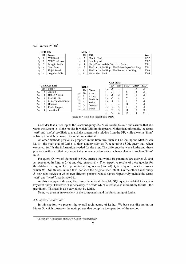
well-known IMDB3.

PERSONID Name

t1 1 Will Smitht2 2 Will Theakstont3 3 Maggie Smitht4 4 Sean Beant5 5 Elijah Woodt6 6 Angelina Jolie

MOVIEID Title Year

t7 7 Men in Black 1997t8 8 I am Legend 2007t9 9 Harry Potter and the Sorcerer’s Stone 2001t10 7 The Lord of the Rings: The Fellowship of the Ring 2001t11 11 The Lord of the Rings: The Return of the King 2003t12 12 Mr. & Mrs. Smith 2005

CHARACTERID Name

t13 13 Agent Jt14 14 Robert Nevillet15 15 Marcus Flintt16 16 Minerva McGonagallt17 17 Boromirt18 18 Frodo Bagginst19 19 Jane Smith

ROLEID Name

t20 20 Actort21 21 Actresst22 22 Producert23 23 Writert24 24 Directort25 25 Editor

CASTINGID PID MID ChID RID

t26 26 1 7 13 20t27 27 1 8 14 20t28 28 2 9 15 20t29 29 3 9 16 21t30 30 4 10 17 20t31 31 4 11 17 20t32 32 5 10 18 20t33 33 5 11 18 20t34 34 6 12 19 21

Figure 1: A simplified excerpt from IMDB

Consider that a user inputs the keyword query Q=“will smith films” and assume that shewants the system to list the movies in which Will Smith appears. Notice that, informally, the terms“will” and “smith” are likely to match the contents of a relation from the DB, while the term “films”is likely to match the name of a relation or attribute.

As other methods previously proposed in the literature, such as CNGen [4] and MatCNGen[2, 11], the main goal of Lathe is, given a query such as Q, generating a SQL query that, whenexecuted, fulfills the information needed for the user. The difference between Lathe and theseprevious methods is that they are not able to handle references to schema elements, such as “films”in Q.

For query Q, two of the possible SQL queries that would be generated are queries S1 andS2, presented in Figures 2 (a) and (b), respectively. The respective results of these queries forthe database of Figure 1 are presented in Figures 2(c) and (d). Query S1 retrieves the movieswhich Will Smith was in, and thus, satisfies the original user intent. On the other hand, queryS2 retrieves movies in which two different persons, whose names respectively include the terms“will” and “smith”, participated in.

As this example indicates, there may be several plausible SQL queries related to a givenkeyword query. Therefore, it is necessary to decide which alternative is more likely to fulfill theuser intent. This task is also carried out by Lathe.

Next, we present an overview of the components and the functioning of Lathe.

3.1. System ArchitectureIn this section, we present the overall architecture of Lathe. We base our discussion on

Figure 3, which illustrates the main phases that comprise the operation of the method.

3Internet Movie Database https://www.imdb.com/interfaces/6

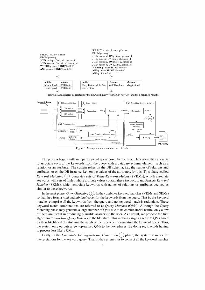
SELECT m.title, p.nameFROM person pJOIN casting c ON p.id=c.person_idJOIN movie m ON m.id = c.movie_idWHERE p.name ILIKE '%will%'AND p.name ILIKE '%smith%';

SELECT m.title, p1.name, p2.nameFROM person p1JOIN casting c1 ON p1.id=c1.person_idJOIN movie m ON m.id = c1.movie_idJOIN casting c2 ON m.id = c2.movie_idJOIN person p2 ON p2.id=c2.person_idWHERE p1.name ILIKE '%will%'AND p2.name ILIKE '%smith%'AND p1.id<>p2.id;

(a) (b)

m.title p.nameMen in Black Will SmithI am Legend Will Smith

m.title p1.name p2.nameHarry Potter and the Sor-cerer’s Stone

Will Theaskton Maggie Smith

(c) (d)

Figure 2: SQL queries generated for the keyword query “will smith movies” and their returned results.

SQL Query

SELECT____FROM______JOIN___ON_WHERE_____

Query Match2

RankingQMsGeneration

Candidate Joining Network3

CJNsGeneration

Ranking

non-voidCJNs

Instance-basedPruning

noyes pruning?

Preprocessing0

RDBMSIndex CreationSchema

Index

ValueIndex

Keyword Match1

VK Match

SK Match

Keyword Query

____________________________________

keywordoccurrences

attribute statistics

keyword frequency

VKMs

SKMs

schemaelements

top-k QMs

earlyevaluation

schema graph

Figure 3: Main phases and architecture of Lathe

The process begins with an input keyword query posed by the user. The system then attemptsto associate each of the keywords from the query with a database schema element, such as arelation or an attribute. The system relies on the DB schema, i.e., the names of relations andattributes, or on the DB instance, i.e., on the values of the attributes, for this. This phase, calledKeyword Matching 1 , generates sets of Value-Keyword Matches (VKMs), which associatekeywords with sets of tuples whose attribute values contain these keywords, and Schema-KeywordMatches (SKMs), which associate keywords with names of relations or attributes deemed assimilar to these keywords.

In the next phase, Query Matching 2 , Lathe combines keyword matches (VKMs and SKMs)so that they form a total and minimal cover for the keywords from the query. That is, the keywordmatches comprise all the keywords from the query and no keyword match is redundant. Thesekeyword match combinations are referred to as Query Matches (QMs). Although the QueryMatching phase may generate a large number of QMs due to its combinatorial nature, only a fewof them are useful in producing plausible answers to the user. As a result, we propose the firstalgorithm for Ranking Query Matches in the literature. This ranking assigns a score to QMs basedon their likelihood of satisfying the needs of the user when formulating the keyword query. Thus,the system only outputs a few top-ranked QMs to the next phases. By doing so, it avoids havingto process less likely QMs.

Lastly, in the Candidate Joining Network Generation 3 phase, the system searches forinterpretations for the keyword query. That is, the system tries to connect all the keyword matches

7

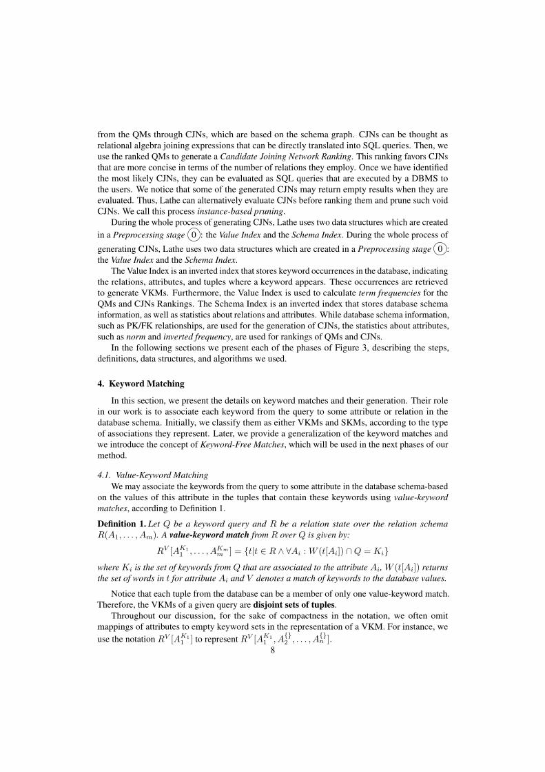
from the QMs through CJNs, which are based on the schema graph. CJNs can be thought asrelational algebra joining expressions that can be directly translated into SQL queries. Then, weuse the ranked QMs to generate a Candidate Joining Network Ranking. This ranking favors CJNsthat are more concise in terms of the number of relations they employ. Once we have identifiedthe most likely CJNs, they can be evaluated as SQL queries that are executed by a DBMS tothe users. We notice that some of the generated CJNs may return empty results when they areevaluated. Thus, Lathe can alternatively evaluate CJNs before ranking them and prune such voidCJNs. We call this process instance-based pruning.

During the whole process of generating CJNs, Lathe uses two data structures which are createdin a Preprocessing stage 0 : the Value Index and the Schema Index. During the whole process of

generating CJNs, Lathe uses two data structures which are created in a Preprocessing stage 0 :the Value Index and the Schema Index.

The Value Index is an inverted index that stores keyword occurrences in the database, indicatingthe relations, attributes, and tuples where a keyword appears. These occurrences are retrievedto generate VKMs. Furthermore, the Value Index is used to calculate term frequencies for theQMs and CJNs Rankings. The Schema Index is an inverted index that stores database schemainformation, as well as statistics about relations and attributes. While database schema information,such as PK/FK relationships, are used for the generation of CJNs, the statistics about attributes,such as norm and inverted frequency, are used for rankings of QMs and CJNs.

In the following sections we present each of the phases of Figure 3, describing the steps,definitions, data structures, and algorithms we used.

4. Keyword Matching

In this section, we present the details on keyword matches and their generation. Their rolein our work is to associate each keyword from the query to some attribute or relation in thedatabase schema. Initially, we classify them as either VKMs and SKMs, according to the typeof associations they represent. Later, we provide a generalization of the keyword matches andwe introduce the concept of Keyword-Free Matches, which will be used in the next phases of ourmethod.

4.1. Value-Keyword MatchingWe may associate the keywords from the query to some attribute in the database schema-based

on the values of this attribute in the tuples that contain these keywords using value-keywordmatches, according to Definition 1.

Definition 1. Let Q be a keyword query and R be a relation state over the relation schemaR(A1, . . . , Am). A value-keyword match from R over Q is given by:

RV [AK11 , . . . , AKm

m ] = {t|t ∈ R ∧ ∀Ai :W (t[Ai]) ∩Q = Ki}

where Ki is the set of keywords from Q that are associated to the attribute Ai, W (t[Ai]) returnsthe set of words in t for attribute Ai and V denotes a match of keywords to the database values.

Notice that each tuple from the database can be a member of only one value-keyword match.Therefore, the VKMs of a given query are disjoint sets of tuples.

Throughout our discussion, for the sake of compactness in the notation, we often omitmappings of attributes to empty keyword sets in the representation of a VKM. For instance, weuse the notation RV [AK1

1 ] to represent RV [AK11 , A

{}2 , . . . , A

{}n ].

8

Example 1. Consider the database instance of Figure 1. The following VKMs can be generatedfor the query “will smith films”.

PERSONV [name{will,smith}]= {t1}PERSONV [name{will}] = {t2}PERSONV [name{smith}] = {t3}

VKMs play a similar role to the tuple-sets from related literature [4, 2]. They are, however,more expressive because they specify which attribute is associated with each keyword. PreviousR-KwS systems based on the DISCOVER system, on the other hand, are unable to create tuple-setsthat span multiple attributes [4, 6, 10]. Example 2 shows a keyword query that includes more thanone attribute.

Example 2. Consider the query “lord rings 2001” whose intent is to return which Lord of theRings movie was launched in 2001. We can represent it with the following value-keyword match:

MOV IEV [title{lord,rings}, year{2001}]= {t10}

The generation of VKMs uses a structure we call the Value Index. This index stores theoccurrences of keywords in the database, indicating the relations and tuples a keyword appears andwhich attributes are mapped to the keyword. Lathe creates the Value Index during a preprocessingphase that scans all target relations only once. This phase comes before the query processingand it is not expected to be repeated frequently. As a result, without further interaction with theDBMS, answers are generated for each query. The Value Index has following the structure, whichis shown in Example 3.

IV = {term : {relation : {attribute : {tuples}}}}

Example 3. The VKMs presented in Example 1 are based on the following keyword occurrences:.

IV [will] ={PERSON : {name : {t1, t2}}}IV [smith] ={PERSON : {name : {t1, t3}}}IV [smith][PERSON ] ={name : {t1, t3}}IV [smith][PERSON ][name]={t1, t3}

In Lathe, the generation of VKMs is carried out by the VKMGen algorithm, presented indetails in Appendix A.

4.2. Schema-Keyword MatchingWe may associate the keywords from the query to some attribute or relation in the database

schema based on the name of the attribute or relation using Schema-Keyword Matches, accordingto Definition 2. Specifically, our method matches keywords to the names of relations and attributesusing similarity metrics.

Definition 2. Let k ∈ Q be a keyword from the query, R(A1, . . . , Am) be a relation schema. Aschema-keyword match from R over k is given by:

RS [AK11 , . . . , AKm

m ] = {t|t ∈ R ∧ ∀k ∈ Ki : sim(Ai, k) ≥ ε}9

where 1 ≤ i ≤ m, Ki is the set of keywords from Q that are associated with the schema elementAi, sim(Ai, k) gives the similarity between the name of a schema element Ai and the keyword k,which must be above a threshold ε, and S denotes a match of keywords to the database schema.

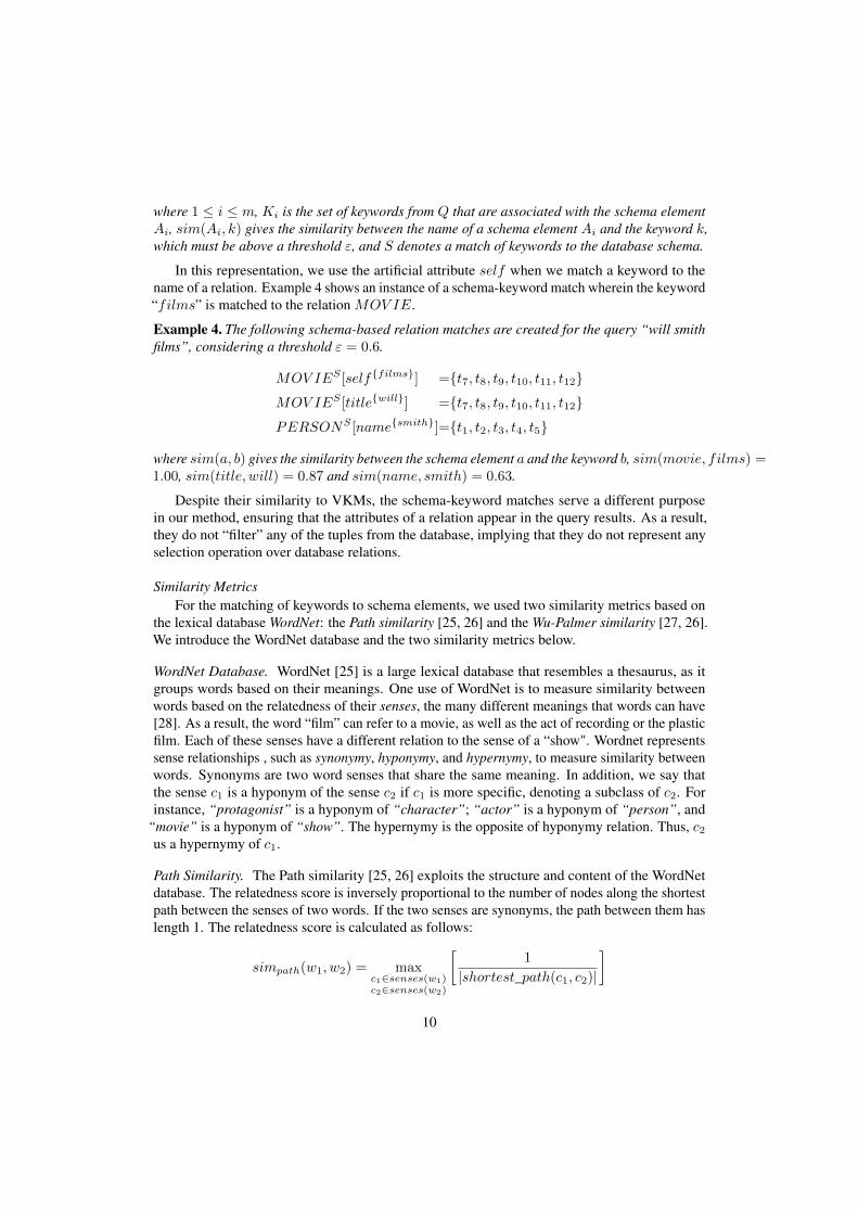
In this representation, we use the artificial attribute self when we match a keyword to thename of a relation. Example 4 shows an instance of a schema-keyword match wherein the keyword“films” is matched to the relation MOV IE.

Example 4. The following schema-based relation matches are created for the query “will smithfilms”, considering a threshold ε = 0.6.

MOV IES [self{films}] ={t7, t8, t9, t10, t11, t12}MOV IES [title{will}] ={t7, t8, t9, t10, t11, t12}PERSONS [name{smith}]={t1, t2, t3, t4, t5}

where sim(a, b) gives the similarity between the schema element a and the keyword b, sim(movie, films) =1.00, sim(title, will) = 0.87 and sim(name, smith) = 0.63.

Despite their similarity to VKMs, the schema-keyword matches serve a different purposein our method, ensuring that the attributes of a relation appear in the query results. As a result,they do not “filter” any of the tuples from the database, implying that they do not represent anyselection operation over database relations.

Similarity MetricsFor the matching of keywords to schema elements, we used two similarity metrics based on

the lexical database WordNet: the Path similarity [25, 26] and the Wu-Palmer similarity [27, 26].We introduce the WordNet database and the two similarity metrics below.

WordNet Database. WordNet [25] is a large lexical database that resembles a thesaurus, as itgroups words based on their meanings. One use of WordNet is to measure similarity betweenwords based on the relatedness of their senses, the many different meanings that words can have[28]. As a result, the word “film” can refer to a movie, as well as the act of recording or the plasticfilm. Each of these senses have a different relation to the sense of a “show". Wordnet representssense relationships , such as synonymy, hyponymy, and hypernymy, to measure similarity betweenwords. Synonyms are two word senses that share the same meaning. In addition, we say thatthe sense c1 is a hyponym of the sense c2 if c1 is more specific, denoting a subclass of c2. Forinstance, “protagonist” is a hyponym of “character”; “actor” is a hyponym of “person”, and

“movie” is a hyponym of “show”. The hypernymy is the opposite of hyponymy relation. Thus, c2us a hypernymy of c1.

Path Similarity. The Path similarity [25, 26] exploits the structure and content of the WordNetdatabase. The relatedness score is inversely proportional to the number of nodes along the shortestpath between the senses of two words. If the two senses are synonyms, the path between them haslength 1. The relatedness score is calculated as follows:

simpath(w1, w2) = maxc1∈senses(w1)c2∈senses(w2)

[1

|shortest_path(c1, c2)|

]

10

Wu-Palmer Similarity. The Wu-Palmer measure (WUP) [27, 26] calculates relatedness by consid-ering the depths of the two synsets c1 and c2 in the WordNet taxonomies, along with the depth ofthe Least Common Subsumer(LCS). The most specific synset c3 is the LCS, which is the ancestorof both synsets c1 and c2. Because the depth of the LCS is never zero, the score can never be zero(the depth of the root of a taxonomy is one). Also, the score is 1 if the two input synsets are thesame. The WUP similarity for two words w1 and w2 is given by:

simwup(w1, w2) = maxc1∈senses(w1)c2∈senses(w2)

[2× depth(lcs(c1, c2))

depth(c1, c2)

]As in the case of VKMs, we detail the SKMGen algorithm used in Lathe in Appendix B.

4.3. Generalization of Keyword MatchesInitially, we presented Definitions 1 and 2 which, respectively, introduce VKMs and SKMs.

We chose to explain the specificity of these concepts separately for didactic purposes. Theyare, however, both components of a broader concept, Keyword Match (KM), which we define inDefinition 3. In the following phases, this generalization will be useful when merging VKMs andSKMs.

Definition 3. Let Q be a keyword query and R be a relation state over the relation schemaR(A1, . . . , Am). Let VKM = RV [A

KS1

1 , . . . , AKS

mm ] be a value-keyword match from R over Q.

Let SKM = RS [AKS

11 , . . . , A

KSm

m ] be a schema-keyword match from R over Q. A general keywordmatch from R over Q is given by:

RS [AKS

11 , . . . , A

KSm

m ]V [AKV

11 , . . . , A

KVm

m ] = VKM ∩ SKM

The representations of VKMs and SKMs in the general notation are given as follows:

RS [AK11 , . . . , AKm

m ] = RS [AK11 , . . . , AKm

m ]V [A{}1 , . . . , A

{}m ]

RV [AK11 , . . . , AKm

m ] = RS [A{}1 , . . . , A

{}m ]V [AK1

1 , . . . , AKmm ]

Another concept required for the generation of QMs and CNs is keyword-free matches, whichwe describe in Definition 4. They are KMs that are not associated with any keyword but are usedas auxiliary structures, such as intermediate nodes in CJNs.

Definition 4. We say that a keyword match KM given by:

KM = RS [AKS

11 , . . . , A

KSm

m ]V [AKV

11 , . . . , A

KVm

m ]

is a keyword-free match if, and only if, @KSi 6={} ∧ @KV

i 6={}, where 1 ≤ i ≤ m.

For the sake of simplifying the notation, we will represent a keyword-free match as RS [ ]V [ ]or simply by R.

5. Query Matching

In this section, we describe the processes of generating and ranking QMs, which are combina-tions of the keyword matches generated in the previous phases that comprise every keyword fromthe keyword query.

11

5.1. Query Matches GenerationWe combine the associations present in the KMs to form total and non-redundant answers for

the user. In other words, Lathe looks for KM combinations that satisfy two conditions: (i) everykeyword from the query must appear in at least one of the KMs and (ii) if any KM is removedfrom the combination, the combination no longer meets the first condition. These combinations,called Query Matches (QMs), are described in Definition 5

Definition 5. LetQ be a keyword query. LetM = {KM1, . . . ,KMn} be a set of keyword matchesfor Q in a certain database instance I , where:

KMi =RSi [A

KSi,1

i,1 , . . . , AKS

i,mii,mi

]V [AKV

i,1

i,1 , . . . , AKV

i,mii,mi

]

Also, let CKMi=⋃

1≤j≤mi

X∈{S,V }KX

i,j and CM=⋃

1≤i≤n CKMibe the sets of all keywords associated

with KMi and with M , respectively. We say that M is a query match for Q if, and only if,CM forms a minimal set cover of the keywords in Q. That is, CM = Q and CM\CKMi

6= Q,∀KMi ∈M .

Notice that a QM cannot contain any keyword-free match, as it would not be minimal anymore.Example 5 presents combinations of KMs which are or are not QMs.

Example 5. Considering the KMs from the Examples 1 and 4, only some of the following sets areconsidered QMs for the query “will smith films”:

M1 = {PERSONV [name{will,smith}],MOV IES [self{films}]}M2 = {PERSONV [name{will}], PERSONV [name{smith}],MOV IES [self{films}]}M3 = {PERSONV [name{will}], PERSONV [name{smith}]}M4 = {PERSONV [name{will,smith}],MOV IES [self{films}], CHARACTER}M5 = {PERSONV [name{will,smith}], PERSONV [name{smith}],MOV IES [self{films}]}

The sets M1 and M2 are considered QMs. In contrast, the sets of keyword matches M3, M4 andM5 are not QMs. While M3 does not include all query keywords, M4 and M5 are not minimal,that is, they have unnecessary KMs.

We present the QMGen algorithm for generating QMs in Appendix C.

5.2. Query Matches RankingAs described in Section 3, Lathe performs a ranking of the QMs generated in the previous

step. This ranking is necessary because frequently many QMs are generated, yet, only a few ofthem are useful to produce plausible answers to the user.

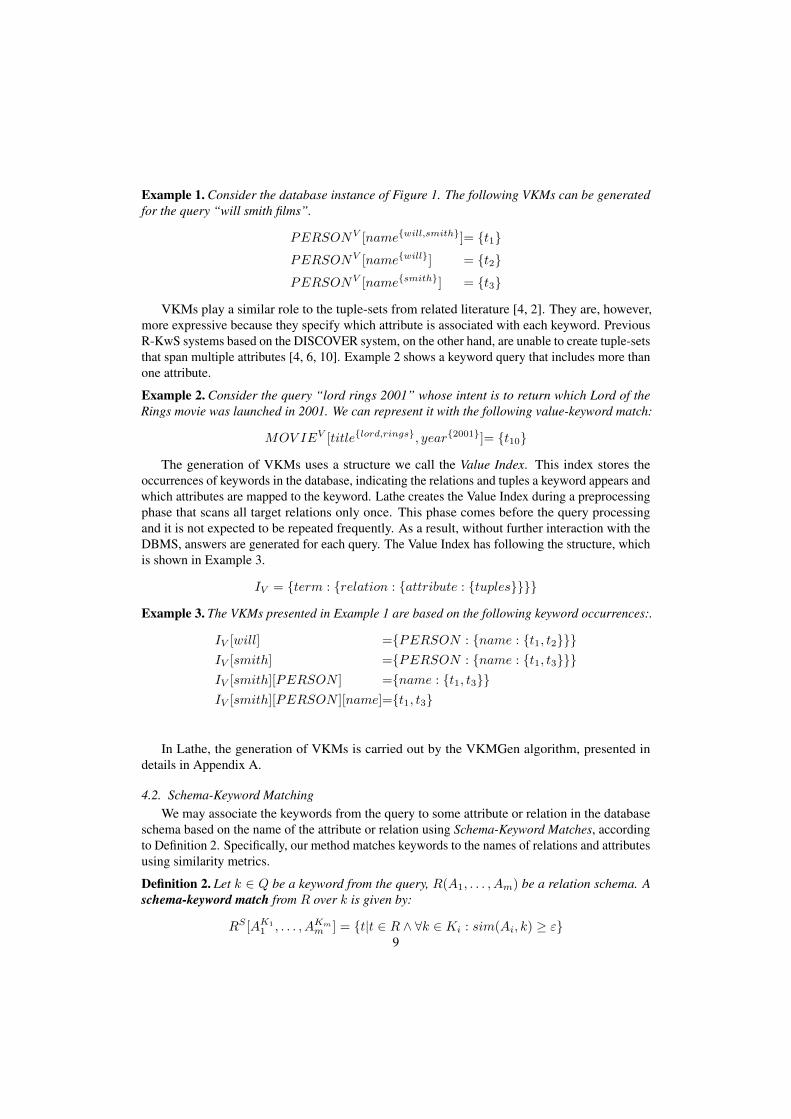
Lathe estimates the relevance of QMs based on a Bayesian Belief Network model for thecurrent state of the underlying database. In practice, this model assess two types of relevancewhen ranking query matches. The the TF-IDF model is used to calculate the value-based score,which adapts the traditional Vector space model to the context of relational databases, as done inLABRADOR [29] and CNRank [10]. The schema-based score, on the other hand, is calculatedby estimating the similarity between keywords and schema elements names.

In Lathe, only the top-k QMs in the ranking are considered in the succeeding phases. Bydoing so, we avoid generating CJNs that are less likely to properly interpret the keyword query.

12

Belief Bayesian Network

We adopt the Bayesian framework proposed by [30] and [31] for modeling distinct IR problems.This framework is simple and allows for the incorporation of features from distinct models intothe same representational scheme. Other keyword search systems, such as LABRADOR [29] andCNRank [10], have also used it.

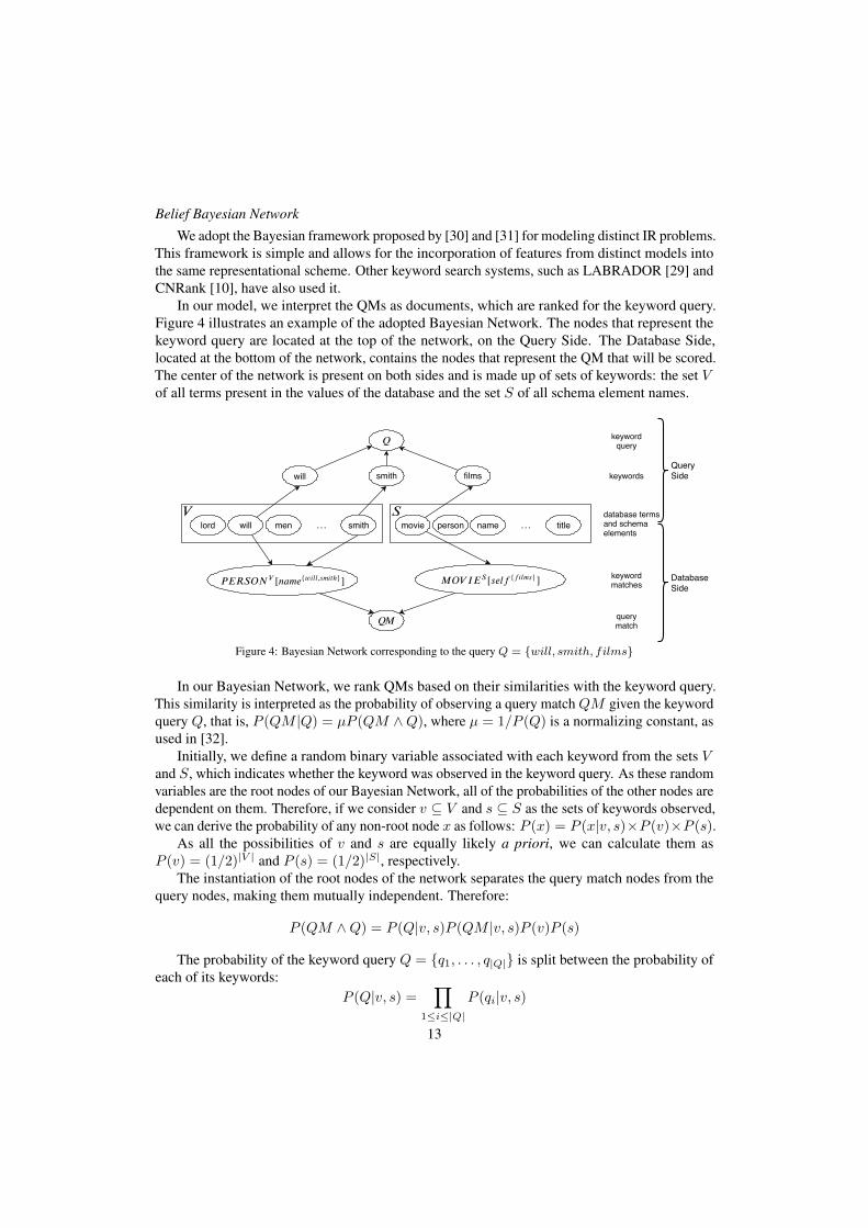
In our model, we interpret the QMs as documents, which are ranked for the keyword query.Figure 4 illustrates an example of the adopted Bayesian Network. The nodes that represent thekeyword query are located at the top of the network, on the Query Side. The Database Side,located at the bottom of the network, contains the nodes that represent the QM that will be scored.The center of the network is present on both sides and is made up of sets of keywords: the set Vof all terms present in the values of the database and the set S of all schema element names.

����� [��� ]� � �{����,����ℎ} ��� � [��� ]�� � {�����}

��

�

will men …

�

smithlord

will smith films

…person name titlemovie�

DatabaseSide

QuerySide

keywordquery

keywords

keywordmatches

querymatch

database termsand schemaelements

Figure 4: Bayesian Network corresponding to the query Q = {will, smith, films}

In our Bayesian Network, we rank QMs based on their similarities with the keyword query.This similarity is interpreted as the probability of observing a query match QM given the keywordquery Q, that is, P (QM |Q) = µP (QM ∧Q), where µ = 1/P (Q) is a normalizing constant, asused in [32].

Initially, we define a random binary variable associated with each keyword from the sets Vand S, which indicates whether the keyword was observed in the keyword query. As these randomvariables are the root nodes of our Bayesian Network, all of the probabilities of the other nodes aredependent on them. Therefore, if we consider v ⊆ V and s ⊆ S as the sets of keywords observed,we can derive the probability of any non-root node x as follows: P (x) = P (x|v, s)×P (v)×P (s).

As all the possibilities of v and s are equally likely a priori, we can calculate them asP (v) = (1/2)|V | and P (s) = (1/2)|S|, respectively.

The instantiation of the root nodes of the network separates the query match nodes from thequery nodes, making them mutually independent. Therefore:

P (QM ∧Q) = P (Q|v, s)P (QM |v, s)P (v)P (s)

The probability of the keyword query Q = {q1, . . . , q|Q|} is split between the probability ofeach of its keywords:

P (Q|v, s) =∏

1≤i≤|Q|

P (qi|v, s)

13

A keyword qi from the query is observed, given the sets s and v, either if qi occurs in the valuesof the database or if qi has a similarity above a threshold ε with a schema element.

P (qi|v, s) = (qi ∈ v) Y (∃k ∈ s : sim(qi, k) ≥ ε)

Similarly, in our network, the probability of a query match QM is splited between theprobability of each of its KMs.

P (QM |v, s) =∏

1≤i≤|QM |

P (KMi|v, s)

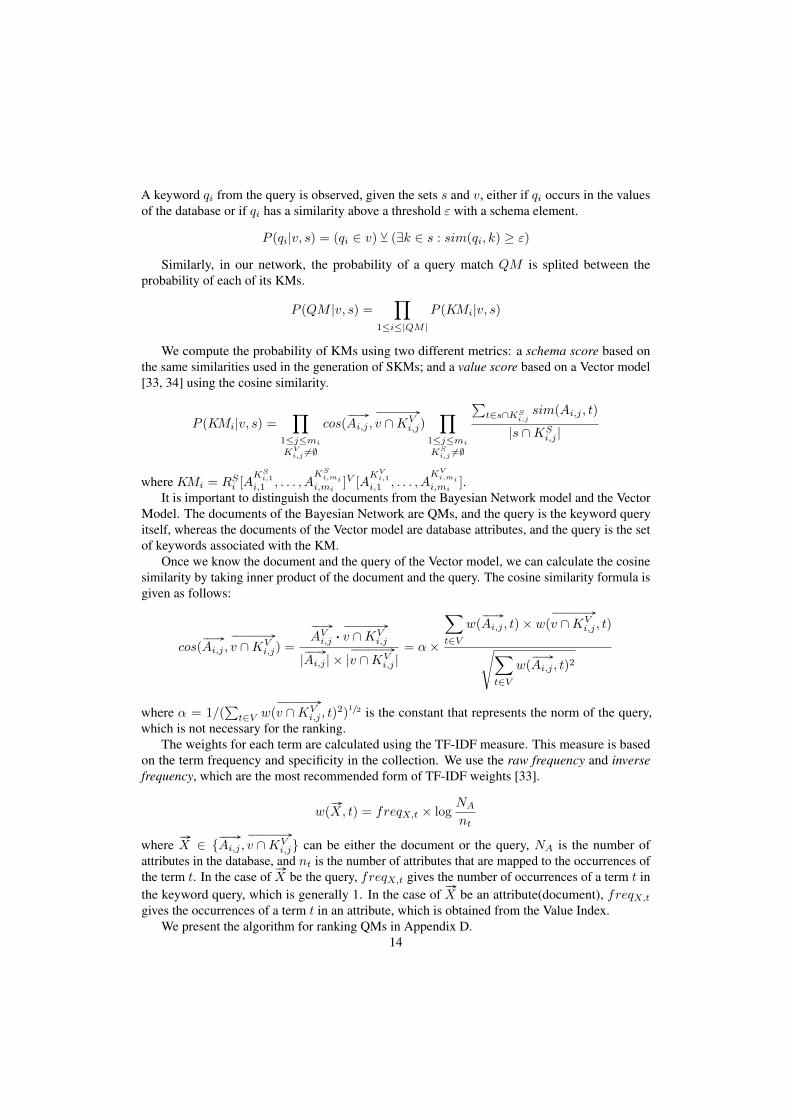
We compute the probability of KMs using two different metrics: a schema score based onthe same similarities used in the generation of SKMs; and a value score based on a Vector model[33, 34] using the cosine similarity.

P (KMi|v, s) =∏

1≤j≤mi

KVi,j 6=∅

cos(# �

Ai,j ,# �

v ∩KVi,j)

∏1≤j≤mi

KSi,j 6=∅

∑t∈s∩KS

i,jsim(Ai,j , t)

|s ∩KSi,j |

where KMi = RSi [A

KSi,1

i,1 , . . . , AKS

i,mii,mi

]V [AKV

i,1

i,1 , . . . , AKV

i,mii,mi

].It is important to distinguish the documents from the Bayesian Network model and the Vector

Model. The documents of the Bayesian Network are QMs, and the query is the keyword queryitself, whereas the documents of the Vector model are database attributes, and the query is the setof keywords associated with the KM.

Once we know the document and the query of the Vector model, we can calculate the cosinesimilarity by taking inner product of the document and the query. The cosine similarity formula isgiven as follows:

cos(# �

Ai,j ,# �

v ∩KVi,j) =

# �

AVi,j ·

# �

v ∩KVi,j

| # �

Ai,j | × |# �

v ∩KVi,j |

= α×

∑t∈V

w(# �

Ai,j , t)× w(# �

v ∩KVi,j , t)√∑

t∈Vw(

# �

Ai,j , t)2

where α = 1/(∑

t∈V w(# �

v ∩KVi,j , t)

2)1/2 is the constant that represents the norm of the query,

which is not necessary for the ranking.The weights for each term are calculated using the TF-IDF measure. This measure is based

on the term frequency and specificity in the collection. We use the raw frequency and inversefrequency, which are the most recommended form of TF-IDF weights [33].

w(#�

X, t) = freqX,t × logNA

nt

where#�

X ∈ { # �

Ai,j ,# �

v ∩KVi,j} can be either the document or the query, NA is the number of

attributes in the database, and nt is the number of attributes that are mapped to the occurrences ofthe term t. In the case of

#�

X be the query, freqX,t gives the number of occurrences of a term t inthe keyword query, which is generally 1. In the case of

#�

X be an attribute(document), freqX,t

gives the occurrences of a term t in an attribute, which is obtained from the Value Index.We present the algorithm for ranking QMs in Appendix D.

14

6. Candidate Joining Networks

In this section we present the details on our method for generating and ranking CandidateJoining Networks (CJNs), which represent different interpretations of the the keyword query. Werecall that our definition of CJNs expands on the definition presented in [4] to support keywordsreferring to schema elements.

The generation of CJNs uses a structure we call a Schema Graph. In this graph, there is a noderepresenting each relation in the database and the edges correspond to the referential integrityconstraints (RIC) in the database schema. In practice, this graph is built in a preprocessing phasebased on information gathered from the database schema.

Definition 6. LetR = {R1, . . . , Rn} be a set of relation schemas from the database. Let E be asubset of the ordered pairs fromR2 given by:

E = {〈Ra, Rb〉|〈Ra, Rb〉 ∈ R2 ∧Ra 6= Rb ∧RIC(Ra, Rb) ≥ 1}

where RIC(Ra, Rb) gives the number of Referential Integrity Constraints from a relation Ra to arelation Rb. We say that a schema graph is an ordered pair GS = 〈R, E〉, whereR is the set ofvertices (nodes) of GS , and E is the set of edges of GS .

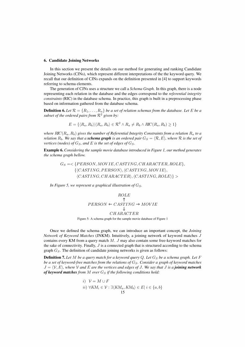
Example 6. Considering the sample movie database introduced in Figure 1, our method generatesthe schema graph bellow.

GS =< {PERSON,MOV IE,CASTING,CHARACTER,ROLE},{〈CASTING,PERSON〉, 〈CASTING,MOV IE〉,〈CASTING,CHARACTER〉, 〈CASTING,ROLE〉} >

In Figure 5, we represent a graphical illustration of GS .

PERSON CASTING MOV IE

CHARACTER

ROLE

Figure 5: A schema graph for the sample movie database of Figure 1

Once we defined the schema graph, we can introduce an important concept, the JoiningNetwork of Keyword Matches (JNKM). Intuitively, a joining network of keyword matches Jcontains every KM from a query match M . J may also contain some free-keyword matches forthe sake of connectivity. Finally, J is a connected graph that is structured according to the schemagraph GS . The definition of candidate joining networks is given as follows:

Definition 7. Let M be a query match for a keyword query Q. Let GS be a schema graph. Let Fbe a set of keyword-free matches from the relations of GS . Consider a graph of keyword matchesJ = 〈V, E〉, where V and E are the vertices and edges of J . We say that J is a joining networkof keyword matches from M over GS if the following conditions hold:

i) V =M ∪ Fii) ∀KMi ∈ V : ∃〈KMa,KMb〉 ∈ E| i ∈ {a, b}

15

iii)∀〈KMa,KMb〉 ∈ E =⇒ ∃〈Ra, Rb〉 ∈ GS

For the sake of simplifying the notation, we will use a graphical illustration to represent CJNs,which is shown in Example 7.

Example 7. Considering the query match M1 previously generated in Example 5, the followingJNKMs can be generated:

J1 = PERSONV [name{will,smith}] CASTING MOV IES [self{films}]

J2 = PERSONV [name{will,smith}] CASTING MOV IES [self{films}]

CHARACTER

The JNKMs J1 and J2 cover the query match M1. The interpretation of J1 looks for themovies of the person will smith. J2 looks for the movies of the person will smith and whichcharacter will smith played in these movies.

Notice that a JNKM might have unnecessary information for the keyword query, which wasthe case of J2 presented in Example 7. One approach to avoid generating unnecessary informationis to generate Minimal Joining Networks of Keyword Matches(MJNKM), which are addressedin Definition 8. Roughly, a MJNKM cannot have any keyword-free match as a leaf, that is, akeyword-free match incident to a single edge.

Definition 8. Let GS be a schema graph. Let M be a query match for a query Q. We say thatJ = 〈V, E〉 from M over GS is minimal joining network of keyword matches (MJNKM) if, andonly if, the following condition holds:

∀KMi ∈ V ( ∃!〈KMa,KMb〉 ∈ E|i ∈ {a, b} =⇒ KMi 6= RSi [ ]

V [ ] )

Example 8. Considering the query match M2 previously generated in Example 5, the followingMJNKMs can be generated:

J3 = PERSONV [name{smith}] CASTING PERSONV [name{will}]

MOV IES [self{films}]

Another issue that a JNKM might have is representing an inconsistent interpretation. Forinstance, it is impossible for J3 presented in Example 8 to return any results from the database. ByDefinition 1, the VKMs PERSONV [name{will}] and PERSONV [name{smith}] are disjoint.However, a tuple from CASTING cannot refer to two different tuples of PERSON . Thus J3is inconsistent. We notice that previous work in literature for CJN generation had addressed thiskind of inconsistency [4, 2]. They did not, however, consider the situation in which there existmore than one RIC from one relation to another. In contrast, based on the theorems and definitionspresented in [4], Lathe proposes a novel approach for checking consistency in CJNs that supportsuch scenarios. Theorem 1 presents a criterion that determines when a JNKM is sound, that is,it can only produce JNTs that do not have more than one occurrences of a tuple. The proof ofTheorem 1 is presented in Appendix E.

16

Theorem 1. Let GS = 〈R, EG〉 be a schema graph. Let J = 〈V, EJ〉 be a joining network ofkeyword matches. We say that J is sound, that is, it does not have more than one occurrencesof the same tuple for every instance of the database if, and only if, the following condition holds∀KMa ∈ V,∀〈Ra, Rb〉 ∈ EG :

RIC(Ra, Rb) ≥ |{KMc|〈KMa,KMc〉 ∈ EJ ∧Rc = Rb}|

where RIC(Ra, Rb) indicates the number of Referential Integrity Constraints from a relation Ra

to a relation Rb.

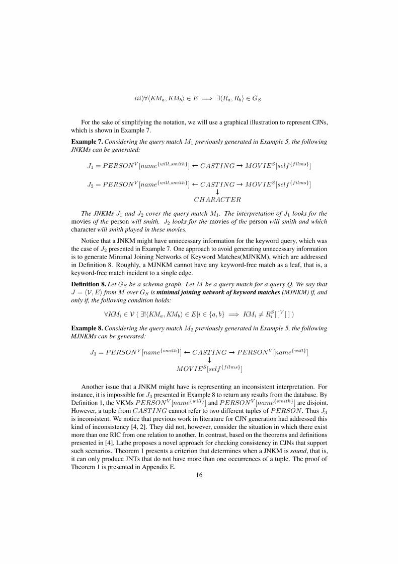
Example 9 presents a JNKM that is sound, although it would be deemed not sound by previousapproaches [4, 2].

Example 9. Consider a simplified excerpt from the MONDIAL database [35], presented in Fig-ure 6. As there exists 2 RICs from the relation BORDER to COUNTRY , represented by theattributes Ctry1_Code e Ctry2_Code, a tuple from BORDER can be joined to at most twodistinct tuples from Country, which is the case of t35 ./ t38 ./ t36. Thus, the following MJNKMis sound:

J4 = COUNTRY V [name{colombia}] BORDER COUNTRY V [name{brazil}]

COUNTRYCode Name Capital_ID

t35 CO Colombia 1t36 BR Brazil 2t37 PE Peru 3

BORDERCtry1_Code Ctry2_Code Length

t38 CO BR 1643t39 PE BR 1560

CITYID Name Population

t40 1 Bogota 1643t41 2 Brasilia 1560t42 3 Lima 1560

Figure 6: A simplified excerpt from MONDIAL

Finally, Definition 9 describes a Candidate Joining Network (CJN), which is roughly a soundminimal joining network of keyword matches.

Definition 9. Let M be a query match for the keyword query Q. Let GS be a schema graph. LetCJN be a joining network of keyword matches from M over GS given by CJN = 〈V, E〉. We saythat CJN is a candidate joining network if, and only if, CJN is minimal and sound.

Example 10. Considering the query match M2 previously generated in Example 5, the followingCJN can be generated:

CJN1 =MOV IES [self{films}] CASTING PERSONV [name{will}]

CASTING PERSONV [name{smith}]

The candidate joining networks CJN1 covers the query match M2. CJN1 is a minimal and soundJNKM. The interpretation of CJN1 searches for the movies where both persons “will” (e.g. WillTheakston) and “smith” (e.g. Maggie Smith) participate in. The two keyword-free matches fromthe CASTING are treated as different nodes in the candidate joining network CJN1.

The details on how we generate CJNs in Lathe are described by the CNKMGen Algorithm inAppendix F.

17

6.1. Candidate Joining Network RankingIn this section, we present CJNKMRank, a novel ranking of CJNs based on the ranking of

QMs. This ranking is necessary because often many CJNs are generated, yet, only a few of themare indeed useful to produce relevant answers.

We present in Section 5.2 a QM ranking that advances the majority of the features present inthe ranking of CJNs of other proposed systems, such as CNRank [10]. Thus, we can exploit thescores of the QMs to rank the CJNs. For this reason, CJNKMRank provides a straightforward yeteffective ranking of candidate joining networks.

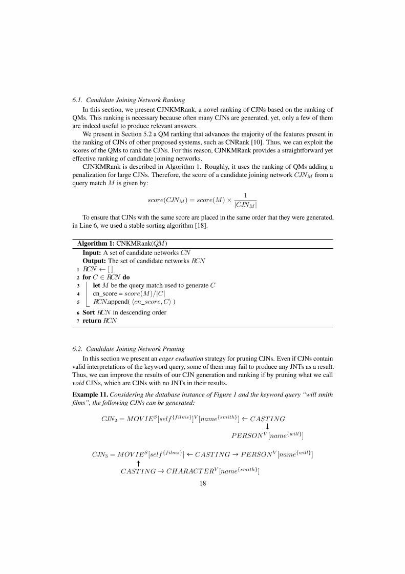
CJNKMRank is described in Algorithm 1. Roughly, it uses the ranking of QMs adding apenalization for large CJNs. Therefore, the score of a candidate joining network CJNM from aquery match M is given by:

score(CJNM ) = score(M)× 1

|CJNM |

To ensure that CJNs with the same score are placed in the same order that they were generated,in Line 6, we used a stable sorting algorithm [18].

Algorithm 1: CNKMRank(QM )Input: A set of candidate networks CNOutput: The set of candidate networks RCN

1 RCN ← [ ]2 for C ∈ RCN do3 let M be the query match used to generate C4 cn_score = score(M)/|C|5 RCN.append( 〈cn_score, C〉 )

6 Sort RCN in descending order7 return RCN

6.2. Candidate Joining Network PruningIn this section we present an eager evaluation strategy for pruning CJNs. Even if CJNs contain

valid interpretations of the keyword query, some of them may fail to produce any JNTs as a result.Thus, we can improve the results of our CJN generation and ranking if by pruning what we callvoid CJNs, which are CJNs with no JNTs in their results.

Example 11. Considering the database instance of Figure 1 and the keyword query “will smithfilms”, the following CJNs can be generated:

CJN2 =MOV IES [self{films}]V [name{smith}] CASTING

PERSONV [name{will}]

CJN3 =MOV IES [self{films}] CASTING PERSONV [name{will}]

CASTING CHARACTERV [name{smith}]

18

The interpretation of CJN2 looks for the movies whose name contains the keyword “smith”(e.g. “Mr. & Mrs. Smith”) and in which a person whose contains “will” (e.g. “Will Theakston”)participate in. The interpretation of CJN3 looks for the movies where a person whose namecontains “will” (e.g. “Will Theakston”) played the character “smith” (e.g. “Jane Smith”). Noticethat although the candidate joining networks CJN2 and CJN3 both provide valid interpretationsfor the keyword query, they do not produce any tuples as a result in the given database instance.

As most of the previous work does not rank CJNs but only evaluates them and ranks theirresulting JNTs instead, the pruning of void CJNs has previously never been addressed. Latheemploys a pruning strategy that evaluates CJNs as soon as they are generated, pruning the voidones. This strategy, as demonstrated in our experiments, can significantly improve the quality ofthe CJN generation process, particularly in scenarios where the schema graph contains a largenumber of nodes and edges.

For instance, one of the datasets we use in our experiments, the MONDIAL database, containsa large number of relations and relational integrity constraint (RICs). This results in a schemagraph with several nodes and edges, which, intuitively, incur a large number of possible CJNs fora single QM. In contrast, we discovered that such schema graphs are prone to produce a largenumber of void CJNs. In particular, while approximately 20% of the keyword queries used in ourexperiments required us to consider 9 CJNs per QM, the eager evaluation strategy reduced thisvalue to 2 CJNs per QM.

Notice, however, that to find if some CJN is void, we must execute it as an SQL in the DBMS,which incurs an additional cost and an increase in the CJN generation time. Despite that, we noticein our experiments that the eager evaluation strategy does not necessarily hinder the performanceof a R-KwS system. In fact, the reducing the number of CJNs per QM alone improves the systemefficiency because this parameter influences the CJN generation process. Furthermore, the eagerevaluation advances the CJN evaluation, which is already a required step in the majority of R-KwSsystems in the related work. Lastly, we can set a maximum number of CJNs to probe during theeager evaluation, which limits the increase in CJN generation time.

7. Experiments

In this section, we report a set of experiments performed using datasets and query setspreviously used in similar experiments reported in the literature. Our goal is to evaluate the qualityof the CJN Ranking, the quality QM ranking, and how we can improve the CJN Generation usingan Eager Evaluation strategy.

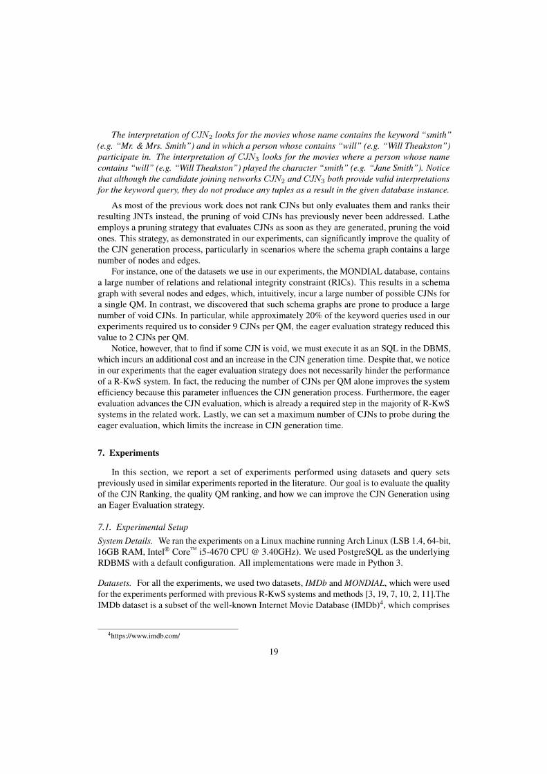
7.1. Experimental Setup

System Details. We ran the experiments on a Linux machine running Arch Linux (LSB 1.4, 64-bit,16GB RAM, Intel® Core™ i5-4670 CPU @ 3.40GHz). We used PostgreSQL as the underlyingRDBMS with a default configuration. All implementations were made in Python 3.

Datasets. For all the experiments, we used two datasets, IMDb and MONDIAL, which were usedfor the experiments performed with previous R-KwS systems and methods [3, 19, 7, 10, 2, 11].TheIMDb dataset is a subset of the well-known Internet Movie Database (IMDb)4, which comprises

4https://www.imdb.com/

19

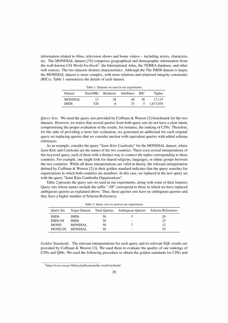
information related to films, television shows and home videos – including actors, characters,etc. The MONDIAL dataset [35] comprises geographical and demographic information fromthe well-known CIA World Factbook5, the International Atlas, the TERRA database, and otherweb sources. The two datasets distinct characteristics. Although the The IMDb dataset is larger,the MONDIAL dataset is more complex, with more relations and relational integrity constraints(RICs). Table 1 summarizes the details of each dataset.

Table 1: Datasets we used in our experiments

Dataset Size(MB) Relations Attributes RIC Tuples

MONDIAL 13 28 48 38 17,115IMDb 528 6 33 5 1,673,076

Query Sets. We used the query sets provided by Coffman & Weaver [3] benchmark for the twodatasets. However, we notice that several queries from both query sets do not have a clear intent,compromising the proper evaluation of the results, for instance, the ranking of CJNs. Therefore,for the sake of providing a more fair evaluation, we generated an additional for each originalquery set replacing queries that we consider unclear with equivalent queries with added schemareferences.

As an example, consider the query “Saint Kitts Cambodia” for the MONDIAL dataset, whereSaint Kitts and Cambodia are the names of the two countries. There exist several interpretations ofthis keyword query, each of them with a distinct way to connect the tuples corresponding to thesecountries. For example, one might look for shared religions, languages, or ethnic groups betweenthe two countries. While all these interpretations are valid in theory, the relevant interpretationdefined by Coffman & Weaver [3] in their golden standard indicates that the query searches fororganizations in which both countries are members. In this case, we replaced in the new query setwith the query "Saint Kitts Cambodia Organizations".

Table 2 presents the query sets we used in our experiments, along with some of their features.Query sets whose names include the suffix “-DI” correspond to those in which we have replacedambiguous queries as explained above. Thus, these queries sets have no ambiguous queries andthey have a higher number of Schema References.

Table 2: Query sets we used in our experiments

Query Set Target Dataset Total Queries Ambiguous Queries Schema References

IMDb IMDb 50 5 20IMDb-DI IMDb 50 - 25MOND MONDIAL 50 7 12MOND-DI MONDIAL 50 - 19

Golden Standards. The relevant interpretations for each query and its relevant SQL results areprovided by Coffman & Weaver [3]. We used them to evaluate the quality of our rankings ofCJNs and QMs. We used the following procedure to obtain the golden standards for CJNs and

5https://www.cia.gov/library/publications/the-world-factbook/

20

QMs. We took the relevant interpretation defined by Coffman & Weaver [3] for each keywordquery and manually identified the CJN that represents this relevant interpretation to define thisCJN as the relevant one. Following that, we took the set of nodes from the relevant CJN that arenot free-keyword matches. This set of KMs corresponds to the relevant QM.

Metrics. We evaluate the ranking of CJNs and QMs using two metrics: Precision at positionranking K (P@K) and Mean Reciprocal Rank (MRR).

Given a keyword query Q , the value of PQ@K is 1 if the target CJN for Q appears in aposition up to K in the ranking, and 0 otherwise. P@K is the average of PQ@K, for all Q in aquery set. With respect to MRR, given a keyword query Q, the value of the reciprocal rankingfor Q, RRQ is given by 1

K , where K is the rank position of the relevant result. Then, the MRRobtained for the queries in a query set is the average of RRQ, for all Q in the query set. Intuitively,the MRR metric measures how close the relevant results are from the first position of the ranking.

Lathe Setup. For the experiments we report here, we set a maximum size for QMs and CJNs of 3and 5, respectively. Also, we consider three important parameters for running Lathe: NQM , themaximum number of QMs considered from the QM ranking; NCJN , the maximum number ofCJNs considered from each QM; and PCJN , the number of CJNs probed per QM by the eagerevaluation. In this context, a setup for Lathe is a triple NQM/NCJN/PCJN . The most commonsetup we used in our experiments is 5/1/9, in which we take the top-5 QMs in the ranking,generate and probe up to 9 CJNs for each QM, and take only the first non-empty CJN, if any,from each QM. We call this the default setup. Later in this section, we will discuss how theseparameters affect the effectiveness and the performance of Lathe, as well as why we use thedefault configuration.

All the resources, including source code, query sets, datasets and golden standards used in ourexperiments are available at https://github.com/pr3martins/Lathe.

7.2. General Results

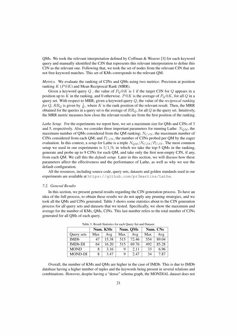
In this section, we present general results regarding the CJN generation process. To have anidea of the full process, to obtain these results we do not apply any pruning strategies, and wetook all the QMs and CJNs generated. Table 3 shows some statistics about to the CJN generationprocess for all query sets and datasets that we tested. Specifically, we show the maximum andaverage for the number of KMs, QMs, CJNs. This last number refers to the total number of CJNsgenerated for all QMs of each query.

Table 3: Result Statistics for each Query Set and Dataset.

Num. KMs Num. QMs Num. CNsQuery sets Max Avg Max Avg Max AvgIMDb 47 15.38 515 72.46 554 89.04IMDb-DI 64 16.20 515 69.76 492 85.28MOND 8 3.16 9 2.11 33 6.96MOND-DI 8 3.47 9 2.47 34 7.87

Overall, the number of KMs and QMs are higher in the case of IMDb. This is due to IMDbdatabase having a higher number of tuples and the keywords being present in several relations andcombinations. However, despite having a “dense” schema graph, the MONDIAL dataset does not

21

have a large number of tuples and the keywords are matched to only a few relations, resulting in alower number of KMs and QMs generated.

Regarding the number of CJNs, the results for the IMDb dataset are also higher in comparisonwith the results from the MONDIAL dataset. However, the ratio of the number CJNs to thenumber of QMs is higher in the results for the MONDIAL dataset, which is due to its morecomplex schema graph.

7.3. Comparison with other R-KwS systems

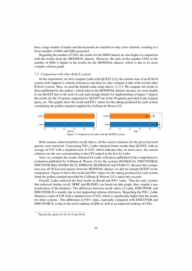
In this experiment, we first compare Lathe with QUEST [12], the current state of art R-KwSsystem with support to schema references and then we also compare Lathe with several otherR-KwS systems. Here, we used the default Lathe setup, that is, 5/1/9. We compare our results tothose published by the authors, which refer to the MONDIAL dataset, because we were unableto run QUEST due to the lack of code and enough details for implementing it Figure 7 depictsthe results for the 35 queries supported by QUEST6out of the 50 queries provided in the originalquery set. The graphs show the recall and P@1 values for the raking produced by each systemconsidering the golden standard supplied by Coffman & Weaver [3].

0.0 0.2 0.4 0.6 0.8 1.0Recall

Lathe

QUEST

0.0 0.2 0.4 0.6 0.8 1.0P@1

Lathe

QUEST

Figure 7: Comparison of Lathe with the QUEST system.

Both systems achieved perfect recall; that is, all the correct solutions for the given keywordqueries were retrieved. Concerning P@1, Lathe obtained better results than QUEST, with anaverage of 0.97 with a standard error of 0.03, which indicates that, in most cases, the correctsolution was the one corresponding to the CJN ranked as the first by Lathe.

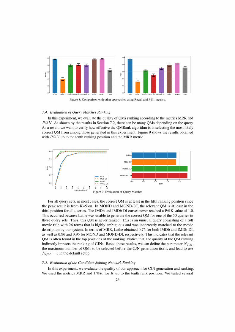
Next, we compare the results obtained for Lathe with those published in the comprehensiveevaluation published by Coffman & Weaver [3] for the systems BANKS[14], DISCOVER[4],DISCOVER-II[6], BANKS-II[15], DPBF[36], BLINKS[16] and STAR[37]. Because this compar-ison uses all 50 keyword queries from the MONDIAL dataset, we did not include QUEST in thecomparison. Figure 8 shows the recall and P@1 values for the raking produced by each systemwhen the golden standard provided by Coffman & Weaver [3] is taken into account.

Overall, Lathe achieved the best results in Recall and P@1 value. That the only systemsthat achieved similar recall, DPBF and BLINKS, are based on data graph, thus, require a ma-terialization of the database. The difference between recall values of Lathe, DISCOVER, andDISCOVER-II is mainly due to not supporting schema references. Regarding the P@1, Latheobtained a value of 0.96 with a standard error of 0.03, which is significantly higher than the resultsfor other systems. This difference in P@1 value, especially compared with DISCOVER andDISCOVER-II, is due to the novel ranking of QMs as well as an improved ranking of CJNs.

6Specifically, queries 01-20, 26-35 and 46-50.

22

LATHE BANKS DISCOVERDISCOVER-II BANKS-II DPBF BLINKS STAR0.0

0.2

0.4

0.6

0.8

1.0

Reca

ll

LATHE BANKS DISCOVERDISCOVER-II BANKS-II DPBF BLINKS STAR0.0

0.2

0.4

0.6

0.8

1.0

P@1

Figure 8: Comparison with other approaches using Recall and P@1 metrics.

7.4. Evaluation of Query Matches Ranking

In this experiment, we evaluate the quality of QMs ranking according to the metrics MRR andP@K. As shown by the results in Section 7.2, there can be many QMs depending on the query.As a result, we want to verify how effective the QMRank algorithm is at selecting the most likelycorrect QM from among those generated in this experiment. Figure 9 shows the results obtainedwith P@K up to the tenth ranking position and the MRR metric.

1 2 3 4 5 6 7 8 9 10Rank Position K

0.6

0.7

0.8

0.9

1.0

P@K

IMDbIMDb-DIMONDMOND-DI

0.0 0.2 0.4 0.6 0.8MRR

IMDb

IMDb-DI

MONDIAL

MONDIAL-DI

Figure 9: Evaluation of Query Matches

For all query sets, in most cases, the correct QM is at least in the fifth ranking position sincethe peak result is from K=5 on. In MOND and MOND-DI, the relevant QM is at least in thethird position for all queries. The IMDb and IMDb-DI curves never reached a P@K value of 1.0.This occurred because Lathe was unable to generate the correct QM for one of the 50 queries inthese query sets. Thus, this QM is never ranked. This is an unusual query consisting of a fullmovie title with 26 terms that is highly ambiguous and was incorrectly matched to the moviedescription by our system. In terms of MRR, Lathe obtained 0.75 for both IMDb and IMDb-DI,as well as 0.96 and 0.95 for MOND and MOND-DI, respectively. This indicates that the relevantQM is often found in the top positions of the ranking. Notice that, the quality of the QM rankingindirectly impacts the ranking of CJNs. Based these results, we can define the parameter NQM ,the maximum number of QMs to be selected before the CJN generation itself, and lead to useNQM = 5 in the default setup.

7.5. Evaluation of the Candidate Joining Network Ranking

In this experiment, we evaluate the quality of our approach for CJN generation and ranking.We used the metrics MRR and P@K for K up to the tenth rank position. We tested several

23

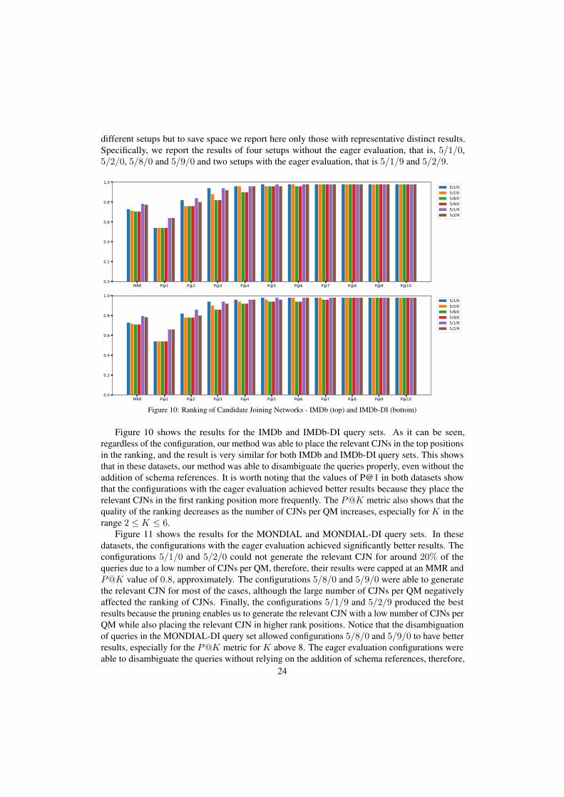
different setups but to save space we report here only those with representative distinct results.Specifically, we report the results of four setups without the eager evaluation, that is, 5/1/0,5/2/0, 5/8/0 and 5/9/0 and two setups with the eager evaluation, that is 5/1/9 and 5/2/9.

MRR P@1 P@2 P@3 P@4 P@5 P@6 P@7 P@8 P@9 [email protected]

0.2

0.4

0.6

0.8

1.05/1/05/2/05/8/05/9/05/1/95/2/9

MRR P@1 P@2 P@3 P@4 P@5 P@6 P@7 P@8 P@9 [email protected]

0.2

0.4

0.6

0.8

1.05/1/05/2/05/8/05/9/05/1/95/2/9

Figure 10: Ranking of Candidate Joining Networks - IMDb (top) and IMDb-DI (bottom)

Figure 10 shows the results for the IMDb and IMDb-DI query sets. As it can be seen,regardless of the configuration, our method was able to place the relevant CJNs in the top positionsin the ranking, and the result is very similar for both IMDb and IMDb-DI query sets. This showsthat in these datasets, our method was able to disambiguate the queries properly, even without theaddition of schema references. It is worth noting that the values of P@1 in both datasets showthat the configurations with the eager evaluation achieved better results because they place therelevant CJNs in the first ranking position more frequently. The P@K metric also shows that thequality of the ranking decreases as the number of CJNs per QM increases, especially for K in therange 2 ≤ K ≤ 6.

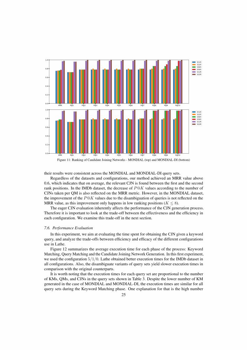
Figure 11 shows the results for the MONDIAL and MONDIAL-DI query sets. In thesedatasets, the configurations with the eager evaluation achieved significantly better results. Theconfigurations 5/1/0 and 5/2/0 could not generate the relevant CJN for around 20% of thequeries due to a low number of CJNs per QM, therefore, their results were capped at an MMR andP@K value of 0.8, approximately. The configurations 5/8/0 and 5/9/0 were able to generatethe relevant CJN for most of the cases, although the large number of CJNs per QM negativelyaffected the ranking of CJNs. Finally, the configurations 5/1/9 and 5/2/9 produced the bestresults because the pruning enables us to generate the relevant CJN with a low number of CJNs perQM while also placing the relevant CJN in higher rank positions. Notice that the disambiguationof queries in the MONDIAL-DI query set allowed configurations 5/8/0 and 5/9/0 to have betterresults, especially for the P@K metric for K above 8. The eager evaluation configurations wereable to disambiguate the queries without relying on the addition of schema references, therefore,

24

MRR P@1 P@2 P@3 P@4 P@5 P@6 P@7 P@8 P@9 [email protected]

0.2

0.4

0.6

0.8

1.05/1/05/2/05/8/05/9/05/1/95/2/9

MRR P@1 P@2 P@3 P@4 P@5 P@6 P@7 P@8 P@9 [email protected]

0.2

0.4

0.6

0.8

1.05/1/05/2/05/8/05/9/05/1/95/2/9

Figure 11: Ranking of Candidate Joining Networks - MONDIAL (top) and MONDIAL-DI (bottom)

their results were consistent across the MONDIAL and MONDIAL-DI query sets.Regardless of the datasets and configurations, our method achieved an MRR value above

0.6, which indicates that on average, the relevant CJN is found between the first and the secondrank positions. In the IMDb dataset, the decrease of P@K values according to the number ofCJNs taken per QM is also reflected on the MRR metric. However, in the MONDIAL dataset,the improvement of the P@K values due to the disambiguation of queries is not reflected on theMRR value, as this improvement only happens in low ranking positions (K ≤ 8).

The eager CJN evaluation inherently affects the performance of the CJN generation process.Therefore it is important to look at the trade-off between the effectiveness and the efficiency ineach configuration. We examine this trade-off in the next section.

7.6. Performance Evaluation

In this experiment, we aim at evaluating the time spent for obtaining the CJN given a keywordquery, and analyze the trade-offs between efficiency and efficacy of the different configurationsuse in Lathe.

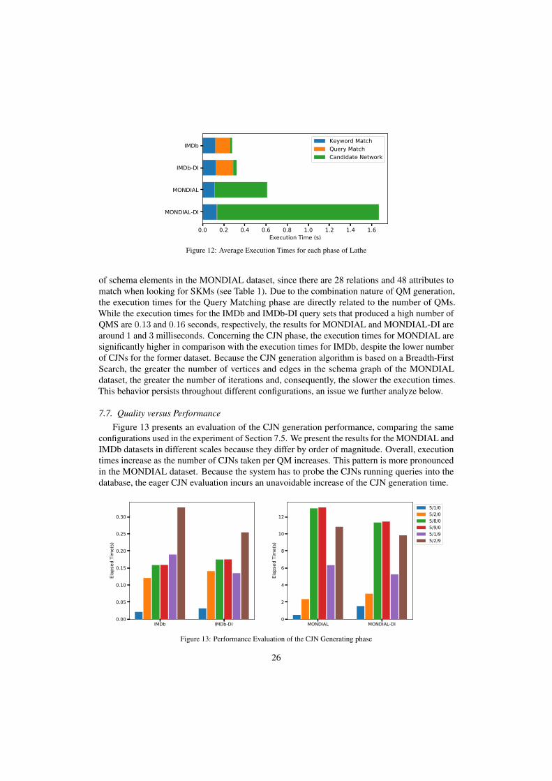
Figure 12 summarizes the average execution time for each phase of the process: KeywordMatching, Query Matching and the Candidate Joining Network Generation. In this first experiment,we used the configuration 5/1/0. Lathe obtained better execution times for the IMDb dataset inall configurations. Also, the disambiguate variants of query sets yield slower execution times incomparison with the original counterparts.

It is worth noting that the execution times for each query set are proportional to the numberof KMs, QMs, and CJNs in the query sets shown in Table 3. Despite the lower number of KMgenerated in the case of MONDIAL and MONDIAL-DI, the execution times are similar for allquery sets during the Keyword Matching phase. One explanation for that is the high number

25

0.0 0.2 0.4 0.6 0.8 1.0 1.2 1.4 1.6Execution Time (s)

IMDb

IMDb-DI

MONDIAL

MONDIAL-DI

Keyword MatchQuery MatchCandidate Network

Figure 12: Average Execution Times for each phase of Lathe

of schema elements in the MONDIAL dataset, since there are 28 relations and 48 attributes tomatch when looking for SKMs (see Table 1). Due to the combination nature of QM generation,the execution times for the Query Matching phase are directly related to the number of QMs.While the execution times for the IMDb and IMDb-DI query sets that produced a high number ofQMS are 0.13 and 0.16 seconds, respectively, the results for MONDIAL and MONDIAL-DI arearound 1 and 3 milliseconds. Concerning the CJN phase, the execution times for MONDIAL aresignificantly higher in comparison with the execution times for IMDb, despite the lower numberof CJNs for the former dataset. Because the CJN generation algorithm is based on a Breadth-FirstSearch, the greater the number of vertices and edges in the schema graph of the MONDIALdataset, the greater the number of iterations and, consequently, the slower the execution times.This behavior persists throughout different configurations, an issue we further analyze below.

7.7. Quality versus Performance

Figure 13 presents an evaluation of the CJN generation performance, comparing the sameconfigurations used in the experiment of Section 7.5. We present the results for the MONDIAL andIMDb datasets in different scales because they differ by order of magnitude. Overall, executiontimes increase as the number of CJNs taken per QM increases. This pattern is more pronouncedin the MONDIAL dataset. Because the system has to probe the CJNs running queries into thedatabase, the eager CJN evaluation incurs an unavoidable increase of the CJN generation time.

IMDb IMDb-DI0.00

0.05

0.10

0.15

0.20

0.25

0.30

Elap

sed

Tim

e(s)

MONDIAL MONDIAL-DI0

2

4

6

8

10

12

Elap

sed

Tim

e(s)

5/1/05/2/05/8/05/9/05/1/95/2/9

Figure 13: Performance Evaluation of the CJN Generating phase

26

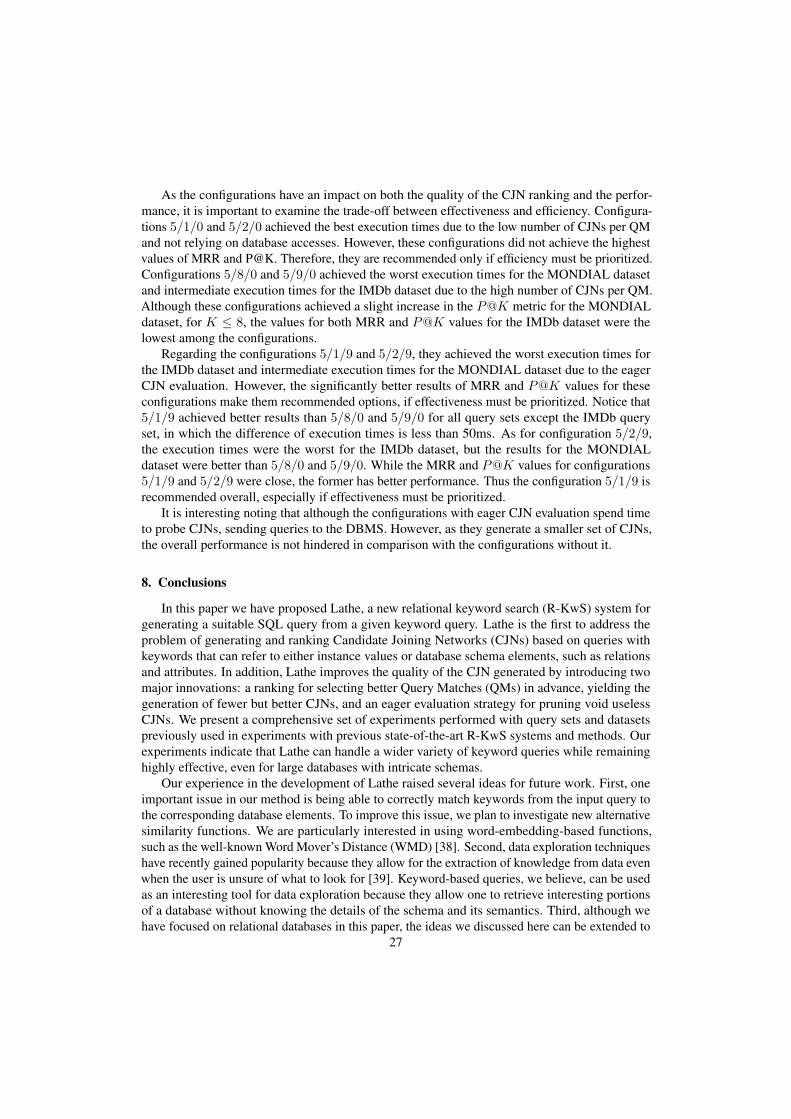
As the configurations have an impact on both the quality of the CJN ranking and the perfor-mance, it is important to examine the trade-off between effectiveness and efficiency. Configura-tions 5/1/0 and 5/2/0 achieved the best execution times due to the low number of CJNs per QMand not relying on database accesses. However, these configurations did not achieve the highestvalues of MRR and P@K. Therefore, they are recommended only if efficiency must be prioritized.Configurations 5/8/0 and 5/9/0 achieved the worst execution times for the MONDIAL datasetand intermediate execution times for the IMDb dataset due to the high number of CJNs per QM.Although these configurations achieved a slight increase in the P@K metric for the MONDIALdataset, for K ≤ 8, the values for both MRR and P@K values for the IMDb dataset were thelowest among the configurations.

Regarding the configurations 5/1/9 and 5/2/9, they achieved the worst execution times forthe IMDb dataset and intermediate execution times for the MONDIAL dataset due to the eagerCJN evaluation. However, the significantly better results of MRR and P@K values for theseconfigurations make them recommended options, if effectiveness must be prioritized. Notice that5/1/9 achieved better results than 5/8/0 and 5/9/0 for all query sets except the IMDb queryset, in which the difference of execution times is less than 50ms. As for configuration 5/2/9,the execution times were the worst for the IMDb dataset, but the results for the MONDIALdataset were better than 5/8/0 and 5/9/0. While the MRR and P@K values for configurations5/1/9 and 5/2/9 were close, the former has better performance. Thus the configuration 5/1/9 isrecommended overall, especially if effectiveness must be prioritized.

It is interesting noting that although the configurations with eager CJN evaluation spend timeto probe CJNs, sending queries to the DBMS. However, as they generate a smaller set of CJNs,the overall performance is not hindered in comparison with the configurations without it.

8. Conclusions

In this paper we have proposed Lathe, a new relational keyword search (R-KwS) system forgenerating a suitable SQL query from a given keyword query. Lathe is the first to address theproblem of generating and ranking Candidate Joining Networks (CJNs) based on queries withkeywords that can refer to either instance values or database schema elements, such as relationsand attributes. In addition, Lathe improves the quality of the CJN generated by introducing twomajor innovations: a ranking for selecting better Query Matches (QMs) in advance, yielding thegeneration of fewer but better CJNs, and an eager evaluation strategy for pruning void uselessCJNs. We present a comprehensive set of experiments performed with query sets and datasetspreviously used in experiments with previous state-of-the-art R-KwS systems and methods. Ourexperiments indicate that Lathe can handle a wider variety of keyword queries while remaininghighly effective, even for large databases with intricate schemas.

Our experience in the development of Lathe raised several ideas for future work. First, oneimportant issue in our method is being able to correctly match keywords from the input query tothe corresponding database elements. To improve this issue, we plan to investigate new alternativesimilarity functions. We are particularly interested in using word-embedding-based functions,such as the well-known Word Mover’s Distance (WMD) [38]. Second, data exploration techniqueshave recently gained popularity because they allow for the extraction of knowledge from data evenwhen the user is unsure of what to look for [39]. Keyword-based queries, we believe, can be usedas an interesting tool for data exploration because they allow one to retrieve interesting portionsof a database without knowing the details of the schema and its semantics. Third, although wehave focused on relational databases in this paper, the ideas we discussed here can be extended to

27

other types of databases as well. Currently, we are extending these ideas to address the so-calleddocument stores, such as the very popular MongoDB7 engine. Our preliminary findings suggestthat because queries of this type are frequently more complex than queries of relational databases,allowing the simplicity of keyword queries may have even more advantages in this context. Finally,we anticipate that keyword queries will be useful as a tool for allowing the seamless integration ofdata from heterogeneous sources, as is the case in the so-called polystores systems and data lakes,which are becoming increasingly popular in recent years. There exist already research proposalsin this direction [40], we believe that the schema graph approach we adopt in our work can behelpful to achieve this goal.

9. Acknowledgments

This research, according for in Article 48 of Decree nº 6.008/2006, was funded by SamsungElectronics of Amazonia Ltda, under the terms of Federal Law nº 8.387/1991, through agreementnº 003, signed with ICOMP/UFAM. It was also supported by the Brazilian funding agencyFAPEAM-POSGRAD 2020 (Resolution 002/2020), the Coordination for the Improvement ofHigher Education Personnel-Brazil (CAPES) financial code 001, by projects SocSens (CAPES/PCGI 88887.130299/2017-01), MMBIAS (FAPESP MCTIC/CGI, 2020/05173-4), and authors’individual grants from CNPq.

Appendix A. VKMGen Algorithm

As shown in Algorithm 2, Lathe retrieves tuples from the database in which the keywordsoccur and uses them to generate value-keyword matches. Initially, the VKMGen Algorithm takesthe occurrences of each keyword from the Value Index and form partial value-keyword matches,which are not guaranteed to be disjoint sets yet (Lines 3-8). The pool of VKMs is represented bythe Hash Table P , whose keys are KMs and values are sets of tuple IDs.

Next, Lathe ensures that VKMs are disjoint sets through the Algorithm 3, VKMInter, which isbased on the ECLAT algorithm [41] for finding frequent itemsets. VKMInter looks for non-emptyintersections of the partial value-keyword matches recursively until all of them are disjoint sets,and thus, proper VKMs. These intersections are calculated as follows:

KM1 ∩KM2 =

{∅ , if Ra 6= Rb

RVab[A

Kab,1

ab,1 , . . . , AKab,m

ab,m ] , if Ra = Rb

where KMx = RVx [A

Kx,1

x,1 , . . . , AKx,mx,m ] for x ∈ {a, b}, and Kab,i = Ka,i ∪Kb,i.

VKMInter uses three hash tables: P , Pnext and R. The pool P contains the partial VKMs ofthe current iteration. The pool Pnext contains the partial VKMs for the next iteration. The pool Rstores the tuple IDs to be removed from the VKMs of P at the end of the current iteration, turningthe partial VKMs into proper value-keyword matches.

VKMInter first defines the hash tables Pnext and R, then initializes R with empty sets (Lines1-4). Next, the algorithm iterates over all pairs {KMa,KMb} of VKMs in P and tries to create anew keyword match KMab, which is the intersection of KMa e KMb (Lines 5-11). If KMab is

7https://www.mongodb.com/

28

Algorithm 2: VKMGen(Q)Input: A keyword query Q={k1, k2, . . . , km}Output: The set of value-keyword matches VK

1 let IV the Value Index2 let P be a Hash Table.3 for keyword ki ∈ Q do4 if ki ∈ IV then5 for relation Rj ∈ IV [ki] do6 for attribute Ak ∈ IV [ki][Rj ] do7 let KM be the partial keyword match RV

j [A{ki}k ]

8 P [KM ]← IV [ki][Rj ][Ak]

9 P ← VKMIter(P )10 for value-keyword match KMu ∈ P do11 VK ← VK ∪ {KMu}12 return VK

valid, that is, if KMa e KMb are VKMs over the same database relation, and the tuples Tab withinKMab are not empty, then we add KMab to the next iteration pool Pnext and add the tuples Tabto R for removal after the iteration (Lines 8-11). After all the possible intersections are processed,VKMInter iterates over R and removes the tuples for each VKM of the pool P , making themproper disjoint keyword matches (Lines 12-16). Lastly, VKMInter recursively process the poolPnext for the next iteration, then it updates and returns the current pool P (Lines 18-19).

After the execution of VKMInter, in Line 9 of VKMGen, we obtained the value-keywordmatches and their tuples. As the sets of tuples are only required for the generation of VKMs,VKMGen generates and outputs the set of value-keyword matches, ignoring the tuples from P(Lines 10-11). From now on, Lathe does not need to manipulate the database tuples or their IDs.

Appendix B. SKMGen Algorithm

The generation of schema-keyword matches uses a structure we call the Schema Index, whichis created in a preprocessing phase, alongside with the Value Index. This index stores informationabout the database schema and statistics about attributes, which are used for the ranking of QMs,which will be explained in Chapter 5. The stored information follows the structure below:

IS = {relation : {attribute : {(norm,maxfrequency)}}}

The generation of SKMs is carried out by Algorithm 4, SKMGen. First, the algorithm iteratesover the relations and attributes from the Schema Index. Then, SKMGen calculates the similaritybetween each keyword and schema element. It only considers the pairs with similarity above adefined threshold ε (Line 8), which are used to generate SKMs (Line 3).

Appendix C. QMGen Algorithm

The generation of query matches is carried out by Algorithm 5, QMGen, which preserves theideas proposed in MatCNGen [2], adapt them to keyword matches instead of tuple-sets. Let VK

29

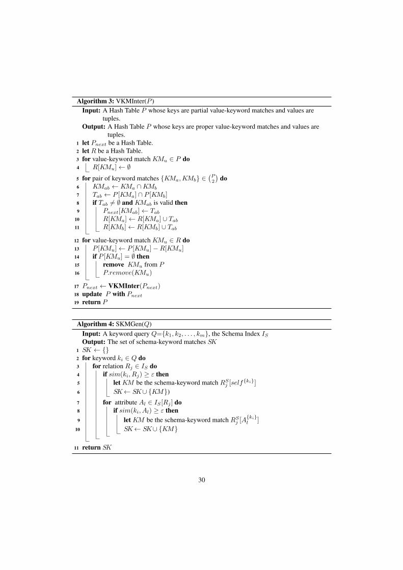
Algorithm 3: VKMInter(P )Input: A Hash Table P whose keys are partial value-keyword matches and values are

tuples.Output: A Hash Table P whose keys are proper value-keyword matches and values are

tuples.1 let Pnext be a Hash Table.2 let R be a Hash Table.3 for value-keyword match KMu ∈ P do4 R[KMu]← ∅5 for pair of keyword matches {KMa,KMb} ∈

(P2

)do

6 KMab ← KMa ∩KMb

7 Tab ← P [KMa] ∩ P [KMb]8 if Tab 6= ∅ and KMab is valid then9 Pnext[KMab]← Tab

10 R[KMa]← R[KMa] ∪ Tab11 R[KMb]← R[KMb] ∪ Tab

12 for value-keyword match KMu ∈ R do13 P [KMu]← P [KMu]−R[KMu]14 if P [KMu] = ∅ then15 remove KMu from P16 P.remove(KMu)

17 Pnext ← VKMInter(Pnext)18 update P with Pnext

19 return P

Algorithm 4: SKMGen(Q)Input: A keyword query Q={k1, k2, . . . , km}, the Schema Index ISOutput: The set of schema-keyword matches SK

1 SK ← {}2 for keyword ki ∈ Q do3 for relation Rj ∈ IS do4 if sim(ki, Rj) ≥ ε then5 let KM be the schema-keyword match RS

j [self{ki}]

6 SK← SK∪ {KM})7 for attribute Al ∈ IS [Rj ] do8 if sim(ki, Al) ≥ ε then9 let KM be the schema-keyword match RS

j [A{ki}l ]

10 SK← SK∪ {KM}

11 return SK

30

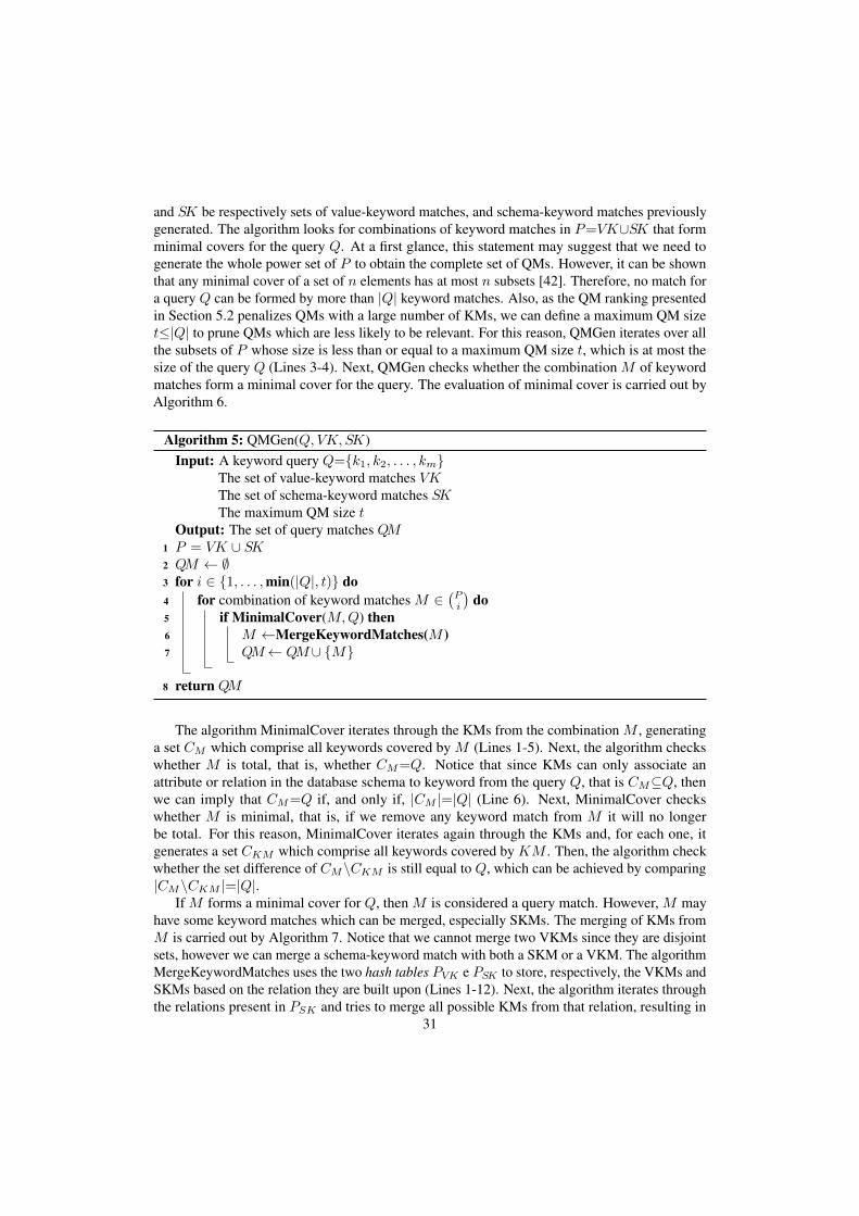
and SK be respectively sets of value-keyword matches, and schema-keyword matches previouslygenerated. The algorithm looks for combinations of keyword matches in P=VK∪SK that formminimal covers for the query Q. At a first glance, this statement may suggest that we need togenerate the whole power set of P to obtain the complete set of QMs. However, it can be shownthat any minimal cover of a set of n elements has at most n subsets [42]. Therefore, no match fora query Q can be formed by more than |Q| keyword matches. Also, as the QM ranking presentedin Section 5.2 penalizes QMs with a large number of KMs, we can define a maximum QM sizet≤|Q| to prune QMs which are less likely to be relevant. For this reason, QMGen iterates over allthe subsets of P whose size is less than or equal to a maximum QM size t, which is at most thesize of the query Q (Lines 3-4). Next, QMGen checks whether the combination M of keywordmatches form a minimal cover for the query. The evaluation of minimal cover is carried out byAlgorithm 6.

Algorithm 5: QMGen(Q,VK, SK)Input: A keyword query Q={k1, k2, . . . , km}

The set of value-keyword matches VKThe set of schema-keyword matches SKThe maximum QM size t

Output: The set of query matches QM1 P = VK ∪ SK2 QM ← ∅3 for i ∈ {1, . . . ,min(|Q|, t)} do4 for combination of keyword matches M ∈

(Pi

)do

5 if MinimalCover(M,Q) then6 M ←MergeKeywordMatches(M )7 QM← QM∪ {M}

8 return QM

The algorithm MinimalCover iterates through the KMs from the combination M , generatinga set CM which comprise all keywords covered by M (Lines 1-5). Next, the algorithm checkswhether M is total, that is, whether CM=Q. Notice that since KMs can only associate anattribute or relation in the database schema to keyword from the query Q, that is CM⊆Q, thenwe can imply that CM=Q if, and only if, |CM |=|Q| (Line 6). Next, MinimalCover checkswhether M is minimal, that is, if we remove any keyword match from M it will no longerbe total. For this reason, MinimalCover iterates again through the KMs and, for each one, itgenerates a set CKM which comprise all keywords covered by KM . Then, the algorithm checkwhether the set difference of CM\CKM is still equal to Q, which can be achieved by comparing|CM\CKM |=|Q|.

If M forms a minimal cover for Q, then M is considered a query match. However, M mayhave some keyword matches which can be merged, especially SKMs. The merging of KMs fromM is carried out by Algorithm 7. Notice that we cannot merge two VKMs since they are disjointsets, however we can merge a schema-keyword match with both a SKM or a VKM. The algorithmMergeKeywordMatches uses the two hash tables PVK e PSK to store, respectively, the VKMs andSKMs based on the relation they are built upon (Lines 1-12). Next, the algorithm iterates throughthe relations present in PSK and tries to merge all possible KMs from that relation, resulting in

31

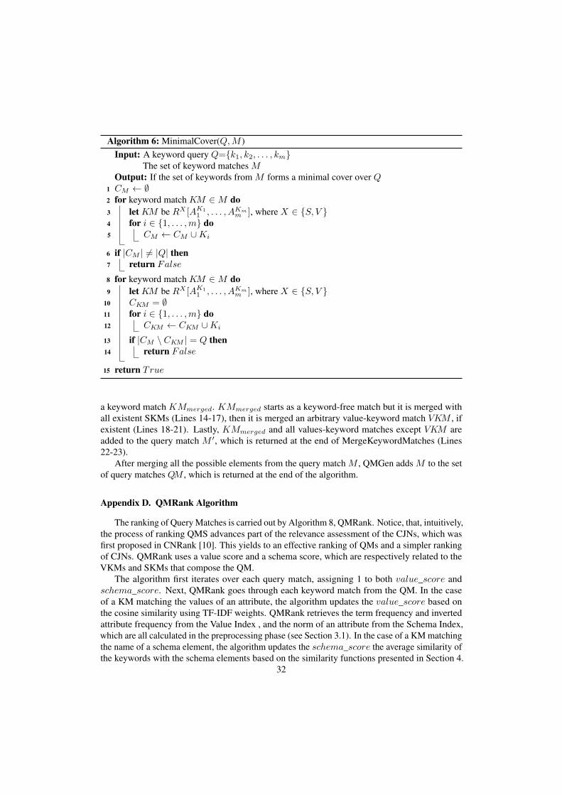
Algorithm 6: MinimalCover(Q,M )Input: A keyword query Q={k1, k2, . . . , km}

The set of keyword matches MOutput: If the set of keywords from M forms a minimal cover over Q

1 CM ← ∅2 for keyword match KM ∈M do3 let KM be RX [AK1

1 , . . . , AKmm ], where X ∈ {S, V }

4 for i ∈ {1, . . . ,m} do5 CM ← CM ∪Ki

6 if |CM | 6= |Q| then7 return False8 for keyword match KM ∈M do9 let KM be RX [AK1

1 , . . . , AKmm ], where X ∈ {S, V }

10 CKM = ∅11 for i ∈ {1, . . . ,m} do12 CKM ← CKM ∪Ki

13 if |CM \ CKM | = Q then14 return False

15 return True

a keyword match KMmerged. KMmerged starts as a keyword-free match but it is merged withall existent SKMs (Lines 14-17), then it is merged an arbitrary value-keyword match VKM , ifexistent (Lines 18-21). Lastly, KMmerged and all values-keyword matches except VKM areadded to the query match M ′, which is returned at the end of MergeKeywordMatches (Lines22-23).

After merging all the possible elements from the query match M , QMGen adds M to the setof query matches QM , which is returned at the end of the algorithm.

Appendix D. QMRank Algorithm

The ranking of Query Matches is carried out by Algorithm 8, QMRank. Notice, that, intuitively,the process of ranking QMS advances part of the relevance assessment of the CJNs, which wasfirst proposed in CNRank [10]. This yields to an effective ranking of QMs and a simpler rankingof CJNs. QMRank uses a value score and a schema score, which are respectively related to theVKMs and SKMs that compose the QM.

The algorithm first iterates over each query match, assigning 1 to both value_score andschema_score. Next, QMRank goes through each keyword match from the QM. In the caseof a KM matching the values of an attribute, the algorithm updates the value_score based onthe cosine similarity using TF-IDF weights. QMRank retrieves the term frequency and invertedattribute frequency from the Value Index , and the norm of an attribute from the Schema Index,which are all calculated in the preprocessing phase (see Section 3.1). In the case of a KM matchingthe name of a schema element, the algorithm updates the schema_score the average similarity ofthe keywords with the schema elements based on the similarity functions presented in Section 4.

32

Algorithm 7: MergeKeywordMatches(Q,M )Input: The set of keyword matches MOutput: The set of keyword matches M ′

1 let PVK be a Hash Table.2 let PSK be a Hash Table.3 for KM ∈M do4 let KM be RX [AK1

1 , . . . , AKmm ], where X ∈ {S, V }

5 PVK [R]← ∅6 PSK [R]← ∅7 for KM ∈M do8 let KM be RX [AK1

1 , . . . , AKmm ], where X ∈ {S, V }

9 if X = S then10 PSK [R]← PSK [R] ∪ {KM}11 else12 PVK [R]← PVK [R] ∪ {KM}

13 M ′ ← ∅14 for R ∈ PSK do15 let KMmerged be a keyword-free match from R16 for SKM ∈ PSK [R] do17 KMmerged ← KMmerged ∩ SKM18 if PVK [R] 6= ∅ then19 let VKM be an element from PVK [R]20 KMmerged ← KMmerged ∩ VKM21 PVK [R]← PVK [R]− {VKM}22 M ′ ←M ′ ∪ {KMmerged} ∪ PVK [R]

23 return M ′

Once the algorithm aggregates the scores of KMs to generate the score of QMs, the final step is tosort them in descending order.

Appendix E. Sound Theorem

Theorem 1. Let GS = 〈R, EG〉 be a schema graph. Let J = 〈V, EJ〉 be a joining network ofkeyword matches. We say that J is sound, that is, it does not have more than one occurrencesof the same tuple for every instance of the database if, and only if, the following condition holds∀KMa ∈ V,∀〈Ra, Rb〉 ∈ EG :

RIC(Ra, Rb) ≥ |{KMc|〈KMa,KMc〉 ∈ EJ ∧Rc = Rb}|

where RIC(Ra, Rb) indicates the number of Referential Integrity Constraints from a relation Ra

to a relation Rb.

Proof. Let Ra and Rb be database relations so that there exists n Referential Integrity Constraint(RICs) from Ra to Rb. Intuitively, a tuple from Ra may refer to at most n tuples from Rb.

33

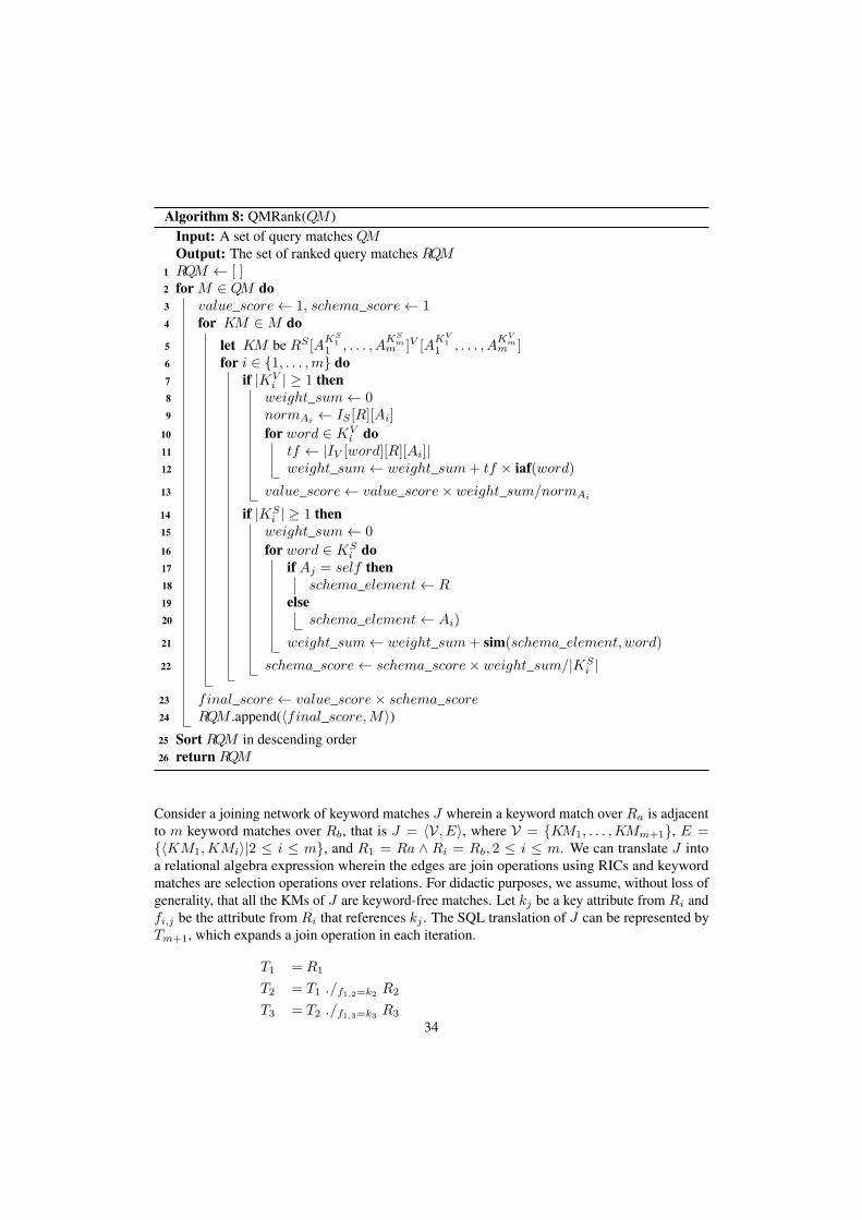
Algorithm 8: QMRank(QM )Input: A set of query matches QMOutput: The set of ranked query matches RQM

1 RQM ← [ ]2 for M ∈ QM do3 value_score← 1, schema_score← 14 for KM ∈M do5 let KM be RS [A

KS1

1 , . . . , AKS

mm ]V [A

KV1

1 , . . . , AKV

mm ]

6 for i ∈ {1, . . . ,m} do7 if |KV

i | ≥ 1 then8 weight_sum← 09 normAi

← IS [R][Ai]

10 for word ∈ KVi do

11 tf ← |IV [word][R][Ai]|12 weight_sum← weight_sum+ tf × iaf(word)13 value_score← value_score× weight_sum/normAi

14 if |KSi | ≥ 1 then

15 weight_sum← 0

16 for word ∈ KSi do

17 if Aj = self then18 schema_element← R19 else20 schema_element← Ai)

21 weight_sum← weight_sum+ sim(schema_element, word)

22 schema_score← schema_score× weight_sum/|KSi |

23 final_score← value_score× schema_score24 RQM .append(〈final_score,M〉)25 Sort RQM in descending order26 return RQM

Consider a joining network of keyword matches J wherein a keyword match over Ra is adjacentto m keyword matches over Rb, that is J = 〈V, E〉, where V = {KM1, . . . ,KMm+1}, E ={〈KM1,KMi〉|2 ≤ i ≤ m}, and R1 = Ra ∧ Ri = Rb, 2 ≤ i ≤ m. We can translate J intoa relational algebra expression wherein the edges are join operations using RICs and keywordmatches are selection operations over relations. For didactic purposes, we assume, without loss ofgenerality, that all the KMs of J are keyword-free matches. Let kj be a key attribute from Ri andfi,j be the attribute from Ri that references kj . The SQL translation of J can be represented byTm+1, which expands a join operation in each iteration.

T1 = R1

T2 = T1 ./f1,2=k2R2

T3 = T2 ./f1,3=k3R3

34

Tn+1= Tn ./f1,n+1=kn+1 Rn+1

Tn+2= Tn+1 ./f1,x=kn+2 Rn+2,where x ∈ {2, . . . , n+ 1}

Notice that by the iteration n + 2, all RICs from Ra to Rb were already used once. Therefore,this expansion require that we use one of the RICs twice, which would lead to redundancy. Forinstance, if assume x = 2, without loss of generality, then:

T2 = T1 ./f1,2=k2R2

Tn+2= Tn+1 ./f1,2=kn+2Rn+2

As the join conditions are stacked in each iteration, we can say that:

f1,2 = k2 ∧ f1,2 = kn+2

which implies that k2 = kn+2 and, thus, all the returning JNTs would have more than oneoccurrence of the same tuple for every instance of the database.

Tm+1= Tm ./f1,x=km+1Rm+1

Appendix F. CJNGen Algorithm

The generation and ranking of CJNs is carried out by Algorithm 9, CJNGen, which uses aBreadth-First Search approach [18] to expand JNKMs until they comprehend all elements from aquery match.

Despite being based on the MatCNGen Algorithm [2], CJNGen provides support for generatingCJNs wherein there exists more than one RIC between one database relation to another, due to thedefinition of soundness presented in Theorem 1. Also, CJNGen does not require an intermediatestructure such as the Match Graph in the MatCNGen system.

We describe CJNGen in Algorithm 9. For each query match, CJNGen generates the candidatejoining networks for this query match using an internal algorithm called CJNInter, which we willfocus on describing in the remainder of this section.

In Algorithm 10, we present CJNInter. This algorithm takes as input a query match M andthe schema graph GS . Next, it chooses a KM from the QM as a starting point, resulting in anunitary graph (Lines 3-4). If the query match M has only one element, we already generated theone possible candidate joining network (Line 6).

Next, the CJNInter initializes a queue D, which is used to store the JNKMs which are notCJNs (Lines 7-8). In Loop 9-27, CJNInter takes one JNKM J from the queue and tries to expandit with KMs. N otice that J can be expanded with incoming and outgoing neighbors, therefore ituses an undirected schema graph GU

S (Line 14). Also, the elements of M can only be added oncein a JNKM but keyword-free matches can be added several times.

35

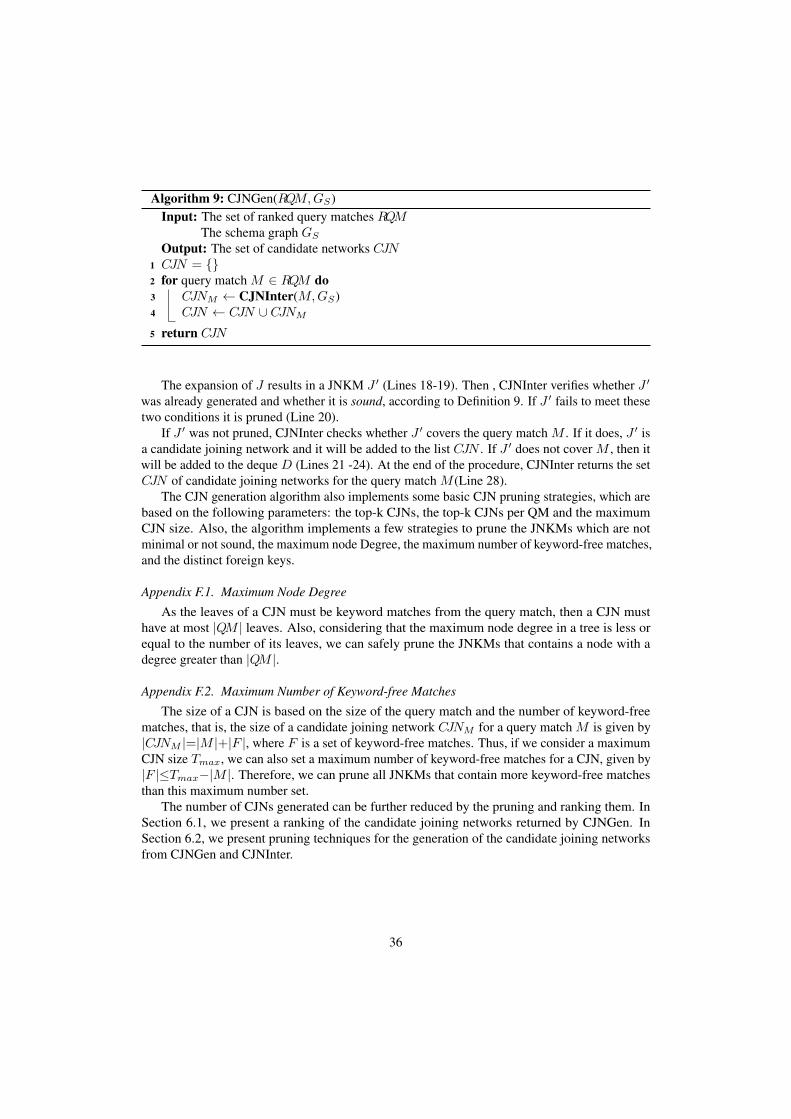
Algorithm 9: CJNGen(RQM,GS)Input: The set of ranked query matches RQM

The schema graph GS

Output: The set of candidate networks CJN1 CJN = {}2 for query match M ∈ RQM do3 CJNM ← CJNInter(M,GS)4 CJN ← CJN ∪ CJNM

5 return CJN

The expansion of J results in a JNKM J ′ (Lines 18-19). Then , CJNInter verifies whether J ′

was already generated and whether it is sound, according to Definition 9. If J ′ fails to meet thesetwo conditions it is pruned (Line 20).

If J ′ was not pruned, CJNInter checks whether J ′ covers the query match M . If it does, J ′ isa candidate joining network and it will be added to the list CJN . If J ′ does not cover M , then itwill be added to the deque D (Lines 21 -24). At the end of the procedure, CJNInter returns the setCJN of candidate joining networks for the query match M (Line 28).

The CJN generation algorithm also implements some basic CJN pruning strategies, which arebased on the following parameters: the top-k CJNs, the top-k CJNs per QM and the maximumCJN size. Also, the algorithm implements a few strategies to prune the JNKMs which are notminimal or not sound, the maximum node Degree, the maximum number of keyword-free matches,and the distinct foreign keys.

Appendix F.1. Maximum Node Degree

As the leaves of a CJN must be keyword matches from the query match, then a CJN musthave at most |QM | leaves. Also, considering that the maximum node degree in a tree is less orequal to the number of its leaves, we can safely prune the JNKMs that contains a node with adegree greater than |QM |.

Appendix F.2. Maximum Number of Keyword-free Matches

The size of a CJN is based on the size of the query match and the number of keyword-freematches, that is, the size of a candidate joining network CJNM for a query match M is given by|CJNM |=|M |+|F |, where F is a set of keyword-free matches. Thus, if we consider a maximumCJN size Tmax, we can also set a maximum number of keyword-free matches for a CJN, given by|F |≤Tmax−|M |. Therefore, we can prune all JNKMs that contain more keyword-free matchesthan this maximum number set.

The number of CJNs generated can be further reduced by the pruning and ranking them. InSection 6.1, we present a ranking of the candidate joining networks returned by CJNGen. InSection 6.2, we present pruning techniques for the generation of the candidate joining networksfrom CJNGen and CJNInter.

36

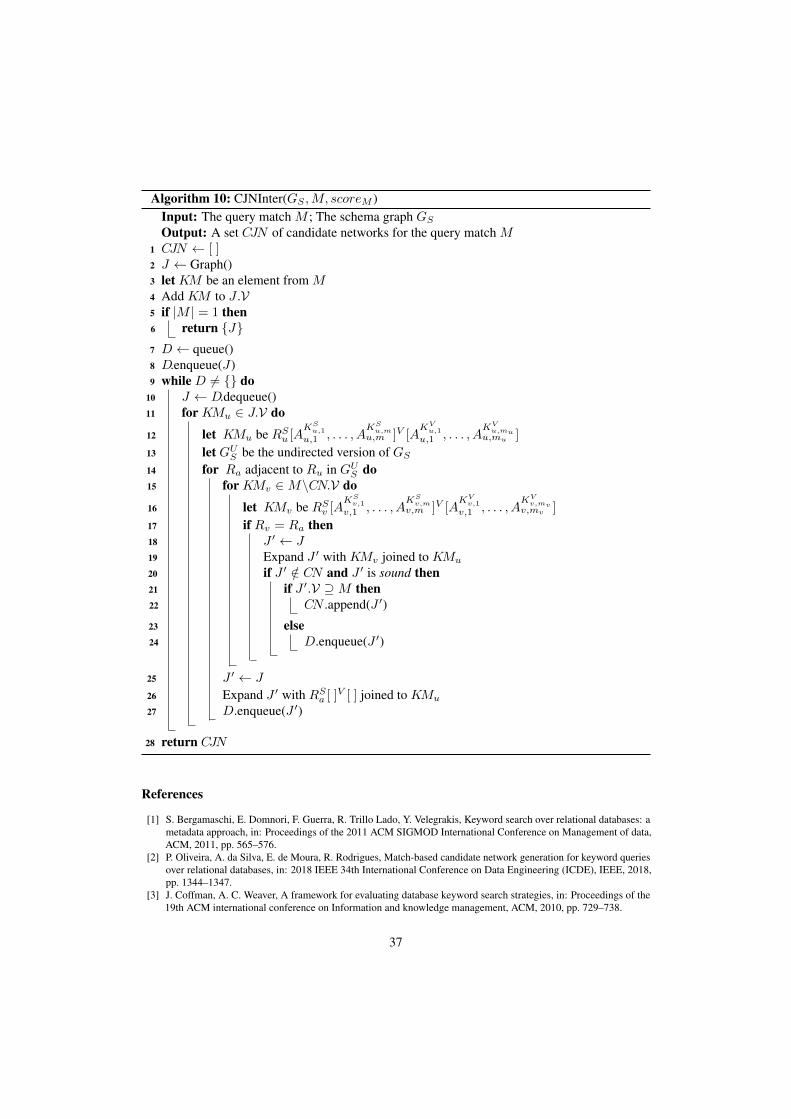
Algorithm 10: CJNInter(GS ,M, scoreM )Input: The query match M ; The schema graph GS

Output: A set CJN of candidate networks for the query match M1 CJN ← [ ]2 J ← Graph()3 let KM be an element from M4 Add KM to J .V5 if |M | = 1 then6 return {J}7 D ← queue()8 D.enqueue(J)9 while D 6= {} do

10 J ← D.dequeue()11 for KMu ∈ J.V do

12 let KMu be RSu [A

KSu,1

u,1 , . . . , AKS

u,mu,m ]V [A

KVu,1

u,1 , . . . , AKV

u,muu,mu ]

13 let GUS be the undirected version of GS

14 for Ra adjacent to Ru in GUS do

15 for KMv ∈M\CN.V do

16 let KMv be RSv [A

KSv,1

v,1 , . . . , AKS

v,mv,m ]V [A

KVv,1

v,1 , . . . , AKV

v,mvv,mv ]

17 if Rv = Ra then18 J ′ ← J19 Expand J ′ with KMv joined to KMu

20 if J ′ /∈ CN and J ′ is sound then21 if J ′.V ⊇M then22 CN .append(J ′)

23 else24 D.enqueue(J ′)

25 J ′ ← J

26 Expand J ′ with RSa [ ]

V [ ] joined to KMu

27 D.enqueue(J ′)

28 return CJN

References

[1] S. Bergamaschi, E. Domnori, F. Guerra, R. Trillo Lado, Y. Velegrakis, Keyword search over relational databases: ametadata approach, in: Proceedings of the 2011 ACM SIGMOD International Conference on Management of data,ACM, 2011, pp. 565–576.

[2] P. Oliveira, A. da Silva, E. de Moura, R. Rodrigues, Match-based candidate network generation for keyword queriesover relational databases, in: 2018 IEEE 34th International Conference on Data Engineering (ICDE), IEEE, 2018,pp. 1344–1347.

[3] J. Coffman, A. C. Weaver, A framework for evaluating database keyword search strategies, in: Proceedings of the19th ACM international conference on Information and knowledge management, ACM, 2010, pp. 729–738.

37

[4] V. Hristidis, Y. Papakonstantinou, Discover: Keyword search in relational databases, in: VLDB’02: Proceedings ofthe 28th International Conference on Very Large Databases, Elsevier, 2002, pp. 670–681.

[5] S. Agrawal, S. Chaudhuri, G. Das, Dbxplorer: A system for keyword-based search over relational databases, in:Proceedings 18th International Conference on Data Engineering, IEEE, 2002, pp. 5–16.

[6] V. Hristidis, L. Gravano, Y. Papakonstantinou, Efficient ir-style keyword search over relational databases, in:Proceedings of the 29th international conference on Very large data bases-Volume 29, VLDB Endowment, 2003, pp.850–861.

[7] Y. Luo, X. Lin, W. Wang, X. Zhou, Spark: top-k keyword query in relational databases, in: Proceedings of the 2007ACM SIGMOD international conference on Management of data, ACM, 2007, pp. 115–126.

[8] J. Coffman, A. C. Weaver, Structured data retrieval using cover density ranking, in: Proceedings of the 2ndInternational Workshop on Keyword Search on Structured Data, ACM, 2010, p. 1.

[9] A. Baid, I. Rae, J. Li, A. Doan, J. Naughton, Toward scalable keyword search over relational data, Proceedings ofthe VLDB Endowment 3 (1-2) (2010) 140–149.

[10] P. Oliveira, A. da Silva, E. de Moura, Ranking candidate networks of relations to improve keyword search overrelational databases, in: 2015 IEEE 31st International Conference on Data Engineering, IEEE, 2015, pp. 399–410.

[11] P. de Oliveira, A. da Silva, E. Moura, R. de Freitas, Efficient match-based candidate network generation for keywordqueries over relational databases, IEEE Transactions on Knowledge and Data Engineering (2020) 1–1.

[12] S. Bergamaschi, F. Guerra, M. Interlandi, R. Trillo-Lado, Y. Velegrakis, Quest: A keyword search system forrelational data based on semantic and machine learning techniques, Proc. VLDB Endow. 6 (12) (2013) 1222–1225.

[13] K. Affolter, K. Stockinger, A. Bernstein, A comparative survey of recent natural language interfaces for databases,The VLDB Journal 28 (5) (2019) 793–819.

[14] B. Aditya, G. Bhalotia, S. Chakrabarti, A. Hulgeri, C. Nakhe, S. Sudarshanxe, et al., Banks: Browsing and keywordsearching in relational databases, in: VLDB’02: Proceedings of the 28th International Conference on Very LargeDatabases, Elsevier, 2002, pp. 1083–1086.

[15] V. Kacholia, S. Pandit, S. Chakrabarti, S. Sudarshan, R. Desai, H. Karambelkar, Bidirectional expansion for keywordsearch on graph databases, in: Proceedings of the 31st international conference on Very large data bases, VLDBEndowment, 2005, pp. 505–516.

[16] H. He, H. Wang, J. Yang, P. S. Yu, Blinks: ranked keyword searches on graphs, in: Proceedings of the 2007 ACMSIGMOD international conference on Management of data, ACM, 2007, pp. 305–316.

[17] F. Liu, C. Yu, W. Meng, A. Chowdhury, Effective keyword search in relational databases, in: Proceedings of the2006 ACM SIGMOD international conference on Management of data, ACM, 2006, pp. 563–574.

[18] T. H. Cormen, C. E. Leiserson, R. L. Rivest, C. Stein, Introduction to algorithms, MIT press, 2009.[19] J. Coffman, A. C. Weaver, An empirical performance evaluation of relational keyword search techniques, IEEE

Transactions on Knowledge and Data Engineering 26 (1) (2012) 30–42.[20] G. Bhalotia, A. Hulgeri, C. Nakhe, S. Chakrabarti, S. Sudarshan, Keyword searching and browsing in databases

using banks, in: Proceedings 18th International Conference on Data Engineering, IEEE, 2002, pp. 431–440.[21] S. Bergamaschi, F. Guerra, S. Rota, Y. Velegrakis, A hidden markov model approach to keyword-based search over

relational databases, in: International Conference on Conceptual Modeling, Springer, 2011, pp. 411–420.[22] S. Tata, G. M. Lohman, Sqak: doing more with keywords, in: Proceedings of the 2008 ACM SIGMOD international

conference on Management of data, ACM, 2008, pp. 889–902.[23] L. Blunschi, C. Jossen, D. Kossmann, M. Mori, K. Stockinger, Soda: Generating sql for business users, Proceedings

of the VLDB Endowment 5 (10) (2012) 932–943.[24] M. S. Ramada, J. C. da Silva, P. de Sá Leitão-Júnior, From keywords to relational database content: A semantic

mapping method, Information Systems 88 (2020) 101460.[25] G. A. Miller, WordNet: An electronic lexical database, MIT press, 1998.[26] T. Pedersen, S. Patwardhan, J. Michelizzi, Wordnet:: Similarity: measuring the relatedness of concepts, in:

Demonstration papers at HLT-NAACL 2004, Association for Computational Linguistics, 2004, pp. 38–41.[27] Z. Wu, M. Palmer, Verbs semantics and lexical selection, in: Proceedings of the 32nd annual meeting on Association

for Computational Linguistics, Association for Computational Linguistics, 1994, pp. 133–138.[28] V. Keselj, Speech and language processing daniel jurafsky and james h. martin (stanford university and university of

colorado at boulder) pearson prentice hall, isbn 978-0-13-187321-6 (2009).[29] F. Mesquita, A. S. da Silva, E. S. de Moura, P. Calado, A. H. Laender, Labrador: Efficiently publishing relational

databases on the web by using keyword-based query interfaces, Information Processing & Management 43 (4)(2007) 983–1004.

[30] B. A. Ribeiro, R. Muntz, A belief network model for ir, in: Proceedings of the 19th annual international ACM SIGIRconference on Research and development in information retrieval, Citeseer, 1996, pp. 253–260.

[31] M. A. P. de Cristo, P. P. Calado, M. d. L. Da Silveira, I. Silva, R. Muntz, B. Ribeiro-Neto, Bayesian belief networksfor ir, International Journal of Approximate Reasoning 34 (2-3) (2003) 163–179.

[32] J. Pearl, Probabilistic reasoning in intelligent systems: networks of plausible inference, Elsevier, 2014.

38

[33] R. Baeza-Yates, B. Ribeiro-Neto, Modern Information Retrieval: The Concepts and Technology Behind Search, 2ndEdition, Addison-Wesley Publishing Company, USA, 2008.

[34] G. Salton, C. Buckley, Term-weighting approaches in automatic text retrieval, Information processing & management24 (5) (1988) 513–523.

[35] W. May, Information extraction and integration with FLORID: The MONDIAL case study, Tech. Rep. 131, Univer-sität Freiburg, Institut für Informatik, available from http://dbis.informatik.uni-goettingen.de/Mondial (1999).

[36] B. Ding, J. X. Yu, S. Wang, L. Qin, X. Zhang, X. Lin, Finding top-k min-cost connected trees in databases, in: 2007IEEE 23rd international conference on data engineering, IEEE, 2007, pp. 836–845.

[37] G. Kasneci, M. Ramanath, M. Sozio, F. M. Suchanek, G. Weikum, Star: Steiner-tree approximation in relationshipgraphs, in: 2009 IEEE 25th International Conference on Data Engineering, IEEE, 2009, pp. 868–879.

[38] M. Kusner, Y. Sun, N. Kolkin, K. Weinberger, From word embeddings to document distances, in: Internationalconference on machine learning, PMLR, 2015, pp. 957–966.

[39] S. Idreos, O. Papaemmanouil, S. Chaudhuri, Overview of data exploration techniques, in: Proceedings of the 2015ACM SIGMOD International Conference on Management of Data, 2015, pp. 277–281.

[40] C. Chanial, R. Dziri, H. Galhardas, J. Leblay, M.-H. Le Nguyen, I. Manolescu, Connectionlens: Finding connectionsacross heterogeneous data sources, Proceedings of the VLDB Endowment (PVLDB) 11 (2018) 4.

[41] M. J. Zaki, Scalable algorithms for association mining, IEEE transactions on knowledge and data engineering 12 (3)(2000) 372–390.

[42] T. Hearne, C. Wagner, Minimal covers of finite sets, Discrete Mathematics 5 (3) (1973) 247–251.

39