Support Vector Regression for Rainfall-Runoff Modeling … · water Article Support Vector Regression for Rainfall-Runoff Modeling in Urban Drainage: A Comparison with the EPA’s

water

Article

Support Vector Regression for Rainfall-RunoffModeling in Urban Drainage: A Comparison with theEPA’s Storm Water Management Model

Francesco Granata *, Rudy Gargano and Giovanni de Marinis

Department of Civil and Mechanical Engineering, University of Cassino and Southern Lazio, via G. Di Biasio 43,03043 Cassino (FR), Italy; [email protected] (R.G.); [email protected] (G.M.)* Correspondence: [email protected]; Tel.: +39-0776-2994-338; Fax: +39-0776-2993-939

Academic Editor: Peter CoombesReceived: 23 November 2015; Accepted: 15 February 2016; Published: 24 February 2016

Abstract: Rainfall-runoff models can be classified into three types: physically based models,conceptual models, and empirical models. In this latter class of models, the catchment is consideredas a black box, without any reference to the internal processes that control the transformation ofrainfall to runoff. In recent years, some models derived from studies on artificial intelligence havefound increasing use. Among these, particular attention should be paid to Support Vector Machines(SVMs). This paper shows a comparative study of rainfall-runoff modeling between a SVM-basedapproach and the EPA’s Storm Water Management Model (SWMM). The SVM is applied in thevariant called Support Vector regression (SVR). Two different experimental basins located in the northof Italy have been considered as case studies. Two criteria have been chosen to assess the consistencybetween the recorded and predicted flow rates: the root-mean square error (RMSE) and the coefficientof determination. The two models showed comparable performance. In particular, both models canproperly model the hydrograph shape, the time to peak and the total runoff. The SVR algorithmtends to underestimate the peak discharge, while SWMM tends to overestimate it. SVR showsgreat potential for applications in the field of urban hydrology, but currently it also has significantlimitations regarding the model calibration.

Keywords: rainfall-runoff; peak discharge; Support Vector regression; Storm Water ManagementModel; SWMM; sewer; urban hydrology

1. Introduction

An efficient drainage network aims to protect people and property within a catchment fromharm [1,2]. The urban rainfall–runoff modeling is a long-debated question. The first hydrologistsattempting to predict the flows that could be expected from a rainfall event also tried to understandhydrological processes, even if their methods were limited by computational techniques and availabledata. The first widely used rainfall-runoff model was the rational method, conceived by T. J. Mulvaneyin 1850 [3]. Even if the model is a single equation, it manages to illustrate most of the problemsthat hydrological modelers have to address: Stormwater is generated by rainfall through a series ofcomplex hydrological processes influenced by many variables. Rainfall-runoff transformation involvestwo main phases: Firstly, hydrological losses occur due to interception, depression storage, infiltrationand evapo-transpiration; secondly, the resulting effective rainfall is transformed into an overland flowby surface routing. Finally, the surface flow is collected by the drainage system.

Water 2016, 8, 69; doi:10.3390/w8030069 www.mdpi.com/journal/water

Water 2016, 8, 69 2 of 13

Stormwater drainage networks sizing is generally based on artificial peak events which are remotefrom real rainfall and runoff processes. Even Mulvaney warned about limitations of peak event-basedapproximations [4].

Existing hydrological models can be classified into three types, namely, (1) physically basedmodels, (2) conceptual models, and (3) empirical models. The latter class of models, unlike the firsttwo categories, involves mathematical equations that are derived from observations of the inputsto and outputs from a catchment basin: Rainfall–runoff modeling is carried out within a purelyanalytical framework based on time-series data. The catchment is considered as a black box, withoutany reference to the physical processes that control the transformation of rainfall to runoff. In recentyears, some models derived from studies on artificial intelligence have found increasing use: artificialneural networks (ANNs) and Support Vector Machines (SVMs).

ANNs [5,6] aim to develop a predictive structure directly from the observational data. They aregenerally presented as a system of interconnected neurons that exchange information between eachother, imitating the working of the brain. The simplest neural networks relate an input signal such asrainfall to an output signal such as runoff by means of a series of weighting functions that may involve anumber of layers of interconnected nodes, including intermediate hidden layers. Several techniques areavailable for determining the appropriate model structure, which will be able to provide a frameworkfor reflecting complexities and nonlinearities in the data as well as some characteristic processes for aparticular catchment.

The SVMs [7,8] are machine-learning algorithms developed by Vapnik and otherresearchers [9–11]. This approach was also at first developed as a way of interpreting sensor data andit involves a two-layer structure. The first layer (Figure 1) is a nonlinear kernel weighting on the inputvariable series, the support vectors, and the second is a weighted sum of the kernel outputs. In manycases, SVMs may be more efficient than ANN methods, once the support vectors and appropriatekernel filters have been determined.

Water 2016, 8, 69 2 of 13

Existing hydrological models can be classified into three types, namely, (1) physically based models, (2) conceptual models, and (3) empirical models. The latter class of models, unlike the first two categories, involves mathematical equations that are derived from observations of the inputs to and outputs from a catchment basin: Rainfall–runoff modeling is carried out within a purely analytical framework based on time-series data. The catchment is considered as a black box, without any reference to the physical processes that control the transformation of rainfall to runoff. In recent years, some models derived from studies on artificial intelligence have found increasing use: artificial neural networks (ANNs) and Support Vector Machines (SVMs).

ANNs [5,6] aim to develop a predictive structure directly from the observational data. They are generally presented as a system of interconnected neurons that exchange information between each other, imitating the working of the brain. The simplest neural networks relate an input signal such as rainfall to an output signal such as runoff by means of a series of weighting functions that may involve a number of layers of interconnected nodes, including intermediate hidden layers. Several techniques are available for determining the appropriate model structure, which will be able to provide a framework for reflecting complexities and nonlinearities in the data as well as some characteristic processes for a particular catchment.

The SVMs [7,8] are machine-learning algorithms developed by Vapnik and other researchers [9–11]. This approach was also at first developed as a way of interpreting sensor data and it involves a two-layer structure. The first layer (Figure 1) is a nonlinear kernel weighting on the input variable series, the support vectors, and the second is a weighted sum of the kernel outputs. In many cases, SVMs may be more efficient than ANN methods, once the support vectors and appropriate kernel filters have been determined.

Figure 1. Network architecture of SVM.

Many researchers have investigated the possibility of addressing hydrological problems using SVMs. Dibike et al. [12] investigated SVMs for rainfall-runoff modeling compared to ANN models. Bray and Han [13] highlighted the difficulties in identifying a suitable model structure and its relevant parameters for rainfall-runoff modeling. Tripathi et al. [14] showed an SVM approach for statistical the downscaling of precipitation at a monthly time scale. Chen et al. [15] used SVMs to predict daily precipitation in the Hanjiang basin. The SVM technique has also been successful recently in solving forestry problems [16], in determining the solar irradiation [17], in predicting the real-time flood [18], and in predicting the daily rainfall-runoff [19]. An extensive review of the SVM applications in the field of hydrology is provided by Raghavendra and Deka [20].

This paper shows a comparative study of rainfall-runoff modeling between a SVM-based approach and the well-known EPA’s Storm Water Management Model (SWMM). SVM is applied in the variant called Support Vector regression (SVR). Two different experimental basins located in the north of Italy have been considered as case studies. Actual observed rainfall and runoff data are used in the study.

Figure 1. Network architecture of SVM.

Many researchers have investigated the possibility of addressing hydrological problems usingSVMs. Dibike et al. [12] investigated SVMs for rainfall-runoff modeling compared to ANN models.Bray and Han [13] highlighted the difficulties in identifying a suitable model structure and its relevantparameters for rainfall-runoff modeling. Tripathi et al. [14] showed an SVM approach for statisticalthe downscaling of precipitation at a monthly time scale. Chen et al. [15] used SVMs to predict dailyprecipitation in the Hanjiang basin. The SVM technique has also been successful recently in solvingforestry problems [16], in determining the solar irradiation [17], in predicting the real-time flood [18],and in predicting the daily rainfall-runoff [19]. An extensive review of the SVM applications in thefield of hydrology is provided by Raghavendra and Deka [20].

Water 2016, 8, 69 3 of 13

This paper shows a comparative study of rainfall-runoff modeling between a SVM-based approachand the well-known EPA’s Storm Water Management Model (SWMM). SVM is applied in the variantcalled Support Vector regression (SVR). Two different experimental basins located in the north of Italyhave been considered as case studies. Actual observed rainfall and runoff data are used in the study.

2. Materials and Methods

2.1. Support Vector Regression

SVR fits a continuous-valued function to data (Figure 2) in a way that shares many of theadvantages of SVM classification. Most algorithms for SVR [21,22] require that training samples areprovided in a single batch. For applications such as on-line time-series prediction, a new model isrequired every time a new sample is added to (or removed from) the training set. Retraining for eachnew data point can be quite expensive.

Water 2016, 8, 69 3 of 13

2. Materials and Methods

2.1. Support Vector Regression

SVR fits a continuous-valued function to data (Figure 2) in a way that shares many of the advantages of SVM classification. Most algorithms for SVR [21,22] require that training samples are provided in a single batch. For applications such as on-line time-series prediction, a new model is required every time a new sample is added to (or removed from) the training set. Retraining for each new data point can be quite expensive.

Figure 2. Example of nonlinear Support Vector regression. Errors do not matter as long as they are less than ε, while the deviations are penalized in a linear fashion, as shown in the top graph, where the “Loss” is the penalty for larger than ε deviations.

The basic idea is the following: Given a training data set {(x1, y1), (x2, y2),…, (xl, yl)} ⊂ X × R, in SVR the goal is to find a function f(x) that has at most ε deviation from the actually obtained targets yi for all the training data and, at the same time, is as flat as possible. The errors that are smaller than ε are not of concern, while the errors greater than ε are unacceptable. In the case of linear functions in the form

( ) ,f x w x b= + (1)

w ∈ X, b ∈ R, and the symbol ,⋅ ⋅ denotes the dot product in X. In order to ensure this, the Euclidean norm ||w||2 need to be minimized. Therefore, this problem can be seen as a convex optimization problem in the form

minimize 21

2w .subject to

,i iy w x b ε− − ≤

, i iw x b y ε + − ≤ (2)

Through Equation (2), it is implicitly assumed that there is a function f that approximates all the pairs (xi, yi) with ε precision. In cases where this is not possible, or a specified error can be tolerated, slack variables ζi, ζi* can be introduced (Figure 2) in the otherwise infeasible constraints of the optimization problem, which can be stated according to the formulation:

minimize ( )2 *

1

12

l

i i

i

w C ξ ξ=

+ + subject to ,i i iy w x b ε ξ− − ≤ +

*, i i iw x b y ε ξ + − ≤ + (3)

i

i*

Error

Loss

i*

f(x)

Figure 2. Example of nonlinear Support Vector regression. Errors do not matter as long as they are lessthan ε, while the deviations are penalized in a linear fashion, as shown in the top graph, where the“Loss” is the penalty for larger than ε deviations.

The basic idea is the following: Given a training data set {(x1, y1), (x2, y2), . . . , (xl , yl)} Ă X ˆ R, inSVR the goal is to find a function f(x) that has at most ε deviation from the actually obtained targets yifor all the training data and, at the same time, is as flat as possible. The errors that are smaller than εare not of concern, while the errors greater than ε are unacceptable. In the case of linear functions inthe form

f pxq “ xw, xy ` b (1)

w P X, b P R, and the symbol x¨, ¨y denotes the dot product in X. In order to ensure this, the Euclideannorm ||w||2 need to be minimized. Therefore, this problem can be seen as a convex optimizationproblem in the form

minimize12‖ w ‖2.subject to

#

yi ´ xw, xiy ´ b ď ε

xw, xiy ` b´ yi ď ε(2)

Through Equation (2), it is implicitly assumed that there is a function f that approximates allthe pairs (xi, yi) with ε precision. In cases where this is not possible, or a specified error can be

Water 2016, 8, 69 4 of 13

tolerated, slack variables ζi, ζi* can be introduced (Figure 2) in the otherwise infeasible constraints of

the optimization problem, which can be stated according to the formulation:

minimize12‖ w ‖2

` Clÿ

i“1

pξi ` ξ˚i q subject to

#

yi ´ xw, xiy ´ b ď ε` ξixw, xiy ` b´ yi ď ε` ξ˚

i(3)

The constant C > 0 directs the choice between the flatness of f and the amount up to whichdeviations larger than ε are tolerated. The optimization problem Equation (3) can be more easilysolved in its dual formulation, utilizing Lagrange multipliers. The first step is to construct a Lagrangefunction from both the objective function and the constraints, introducing a dual set of variables:

L “12‖ w ‖2

` Clř

i“1

`

ξi ` ξ˚i˘

´lř

i“1αi pε` ξi ´ yi ` xw, xiy ` bq´

lř

i“1α˚

i`

ε` ξ˚i ` yi ´ xw, xiy ´ b

˘

´lř

i“1

`

ηiξi ` η˚i ξ˚

i˘

(4)

The dual variables in Equation (4) have to satisfy the conditions αi, α˚i , ηi, η˚

i ě 0, while thepartial derivatives of L with respect to the primal variables

`

w, b, ξi ξ˚i˘

must vanish to reach theoptimal condition:

BLBb“

lÿ

i“1

pα˚i ´ αiq “ 0 (5)

BLBw

“ w´lÿ

i“1

pαi ´ α˚i qxi “ 0 (6)

BLBξ˚

i“ C´ α˚

i ´ η˚i “ 0 (7)

Combining Equations (5)–(7) and Equation (4) leads to the dual optimization problem:

maximize

$

’

’

’

&

’

’

’

%

´12

lř

i,j“1pαi ´ α˚

i qpαj ´ α˚j qxxi, xjy

´εlř

i“1pαi ` α˚

i q `lř

i“1yipαi ´ α˚

j q

subject to

$

’

&

’

%

lř

i“1pαi ´ α˚

i q “ 0

αi, α˚i P r0, Cs

(8)

The dual variables ηi, η˚i do not appear in the dual objective function because they have been

eliminated through Equation (7). Equation (6) can be rewritten as:

w “lÿ

i“1

pαi ´ α˚i qxi (9)

therefore,

f pxq “lÿ

i“1

pαi ´ α˚i qxxi, xy ` b (10)

which is the support vector expansion of the function f, while w can be completely expressed as a linearcombination of the training patterns xi.

The issue of computing b can be addressed by exploiting the Karush-Kuhn-Tuckerconditions [23,24], which state that at the optimal solution the product between dual variables andconstraints has to vanish, that is,

αi pε` ξi ´ yi ` xw, xiy ` bq “ 0α˚

i`

ε` ξ˚i ` yi ´ xw, xiy ´ b

˘

“ 0(11)

Water 2016, 8, 69 5 of 13

andpC´ αiqξi “ 0pC´ α˚

i qξ˚i “ 0

(12)

From that, some important considerations arise. First of all, only samples (xi, yi) withcorresponding αi

* = C are positioned outside the ε-insensitive tube around f. Secondly, αiαi* = 0,

that is a set of dual variables αi, αi*, which are both simultaneously nonzero, does not exist. Finally,

from αi*P (0, C) results ζi

* = 0, and the second factor in Equation (11) has to vanish. Therefore, b can beevaluated by the following:

b “ yi ´ xw, xiy ´ ε

b “ yi ´ xw, xiy ` ε(13)

for αi P (0, C) and αi* P (0, C).

Subsequently, it is necessary to make the Support Vector algorithm nonlinear. This can be obtainedby preprocessing the training patterns xi by a map Φ: XÑF, where F is some feature space [22].The Support Vector algorithm only depends on dot products between the various patterns, so it issufficient to know and use a kernel kpxi, xjq “

@

Φpxiq, ΦpxjqD

instead of Φ(¨) explicitly. This allows usto rewrite the Support Vector algorithm as follows:

maximize

$

’

’

’

&

’

’

’

%

´12

lř

i,j“1pαi ´ α˚

i qpαj ´ α˚j qkpxi, xjq

´εlř

i“1pαi ` α˚

i q `lř

i“1yipαi ´ α˚

j q

subject to

$

’

&

’

%

lř

i“1pαi ´ α˚

i q “ 0

αi, α˚i P r0, Cs

(14)

The expansion of f can now be written as:

f pxq “lÿ

i“1

pαi ´ α˚i qkpxi, xq ` b (15)

Unlike that in the linear case, w is no longer explicitly specified, though uniquely defined. In thenonlinear setting, the optimization problem corresponds to finding the flattest function in featurespace, not in input space. The functions k(xi, xj) corresponding to a dot product in some feature spaceF have to satisfy the Mercer’s condition [22].

The kernel functions commonly used in SVR formulations are:

Linear kpxi, xjq “ xTi xj (16)

Polynomial kpxi, xjq “ pγxTi xj ` rq

d(17)

Radial basis function (RBF) kpxi, xjq “ exp´

´γ‖ xi ´ xj ‖2¯

, γ ą 0 (18)

Sigmoid kpxi, xjq “ tanhpγxTi xj ` rq (19)

A SVR algorithm has been implemented in a computer code written in MATLAB language.A radial basis function has been chosen as kernel. Input vectors contain rainfall and flow observations.However, as highlighted by Bray and Han [13], analysis results show that SVR effectiveness is lessaffected by rainfall and the performance enhancement of the model with increased flow observation ismore significant than the improvement due to increased rainfall observation. An exhaustive search ofan optimum model structure and its parameters is very complicated. It is based on a long and tedioustrial and error iteration procedure, which is very difficult to automate and is omitted here for reasonsof brevity. More details can be found in Bray and Han [13].

Water 2016, 8, 69 6 of 13

The deviation between the target value and the function found by the SVM is controlled by the εparameter. In this study, ε has been finally chosen to be equal to 0.01, while the cost of error C, whichis useful for controlling the smoothness of the function, has been assumed to equal 2.

2.2. SWMM

The well-known SWMM is a dynamic hydrology-hydraulic water quality simulation model.It is used throughout the world for analysis, design and planning related to stormwater runoff,combined and sanitary sewers, and other drainage systems. It can be used for single-event or long-termsimulation [25] of runoff quantity and quality mainly from urban areas. The RUNOFF componentoperates on a collection of subcatchments that receive precipitation and generate runoff and pollutantloads. The ROUTING component transports this runoff through a system of pipes, channels, storage,treatment devices, pumps, and regulators.

The RUNOFF component generates hydrographs by processing rainfall data and a set of physicalcharacteristics describing the catchment basin: area, slope, width, percent impervious, surfaceroughness, depression storage, and infiltration coefficients. The urban basin has to be divided intosub-basins with uniform characteristics. In order to model rainfall-runoff processes, each sub-basin isfurther divided into two parts: the pervious portion and the impervious portion. Each part is modeledas a nonlinear reservoir with a capacity given by the maximum depression storage. Infiltration ismodeled by Horton’s equation, by Green-Ampt’s equation or by SCS Curve Number method.

The ROUTING component models the sewer system as a series of nodes and links. The nodesconsist of manholes, storage units, flow dividers and outfalls, while the links consist of conduits,pumping systems, weirs, orifices and outlets. Surface runoff enters the sewer system at nodes.Runoff transport in sewer system is modeled by the classical De Saint-Venant equations.

Some parameters that characterize the hydrological behavior of the watershed are difficult toevaluate reliably; therefore, a calibration stage to estimate an optimal set of these parameters isessential. An automatic calibration technique has been used in this study. The technique is basedon the optimization method called the complex method developed by Box [26]. The details of theprocedure are shown in Barco et al. [27]. In this work, the following parameters have been consideredin the calibration process: Manning’s coefficients, depression storage for both impervious and perviousarea, and the parameters of the Green-Ampt’s equation (Suction Head Su, Conductivity Ks and InitialDeficit). In order to simplify the calibration process, the width value for each sub-basin has beenmanually evaluated, in accordance with the suggestions of Rossman [25]. The constraints on theparameters were selected based on their physical meaning.

2.3. Case Studies

Two case studies [28] have been considered: the Merate experimental catchment and the CascinaScala experimental catchment (Figure 3).

The Merate experimental catchment is located in the inner city of Merate, in the province of Lecco,30 km far from Milan. The total area of the basin is 93.82 ha, 38% of which is impervious (19% roofsand 19% streets and paved surfaces). The entire basin is divided into three main sub-basins: A1, A2and A3. The average slope of the basin is 2% in the north-south direction. The available experimentaldata refer to the sub-basin A2, which has an area of 20.83 ha, 20% of which is impervious. The basinhas been subdivided in 76 subcatchments. The width of the subcatchments ranges from 31 m to 196 m.

The combined sewerage network in sub-basin A2 is made of 77 concrete conduits, and it has atotal length of 1900 m. The diameters of the pipes range from 300 mm to 800 mm, while the slopes areall quite high. The rainfall on the basin is measured with three rain gauges. The temporal resolution is2 min. In this study, 10 events recorded in Merate have been considered, 8 of which have been used forSVR algorithm training and 2 for testing.

Water 2016, 8, 69 7 of 13Water 2016, 8, 69 7 of 13

Figure 3. Case studies: Merate experimental catchment and Cascina Scala experimental catchment.

The Cascina Scala experimental catchment is a residential district situated in Northern Pavia. The total area of the basin is 14.37 ha, while the contributing area is 11.35 ha, 65% of which is impervious (22.4% roofs and 42.5% streets and paved surfaces), and 35% is pervious. An area of 3.02 ha is not connected to the sewer system. The basin has been subdivided in 42 subcatchments. The width of the subcatchments ranges from 33 m to 201 m.

The combined sewerage network is made of 42 conduits and has a total length of 2045 m, while the slope of the sewer pipes ranges between 0.15% and 1.01%, with an average value weighted on the length of 0.42%. All the sewers are made of concrete pipes. The rainfall on the basin is measured by two rain gauges. The distance between the two rain gauges is 310 m; therefore, the spatial uniformity of the precipitation can be checked and the meteorological volume can be evaluated accurately. The temporal resolution is 2 min. In this research, 20 rainfall-runoff events recorded in Cascina Scala have been considered, 16 of which have been used for SVR training and 4 for testing. Table 1 summarizes the calibrated hydrologic parameters for the two basins.

Table 1. Calibrated parameters for SWMM simulations.

Basin: MERATE n IMP n PERV IMP D.S. PERV D.S. Su Ks i. m. d.

(mm) (mm) (mm) (mm/h) (m/m)

0.13 0.45 1.1 5.5 120 5 0.2 Basin: CASCINA SCALA n IMP n PERV IMP D.S. PERV D.S. Su Ks i. m. d.

(mm) (mm) (mm) (mm/h) (m/m)

0.014 0.4 1.25 2.46 150 7.4 0.15

R1

R2

F

A1

A2

A3

R2

R3

R1

R4

F

N

0 100 m

0 500 m

MERATE

CASCINA SCALA

CASCINA S.

MERATE

N

SEWERAGE NETWORK

WATERSHED

R RAIN GAUGE

F FLOWMETER

A SUBBASIN

Figure 3. Case studies: Merate experimental catchment and Cascina Scala experimental catchment.

The Cascina Scala experimental catchment is a residential district situated in Northern Pavia.The total area of the basin is 14.37 ha, while the contributing area is 11.35 ha, 65% of which is impervious(22.4% roofs and 42.5% streets and paved surfaces), and 35% is pervious. An area of 3.02 ha is notconnected to the sewer system. The basin has been subdivided in 42 subcatchments. The width of thesubcatchments ranges from 33 m to 201 m.

The combined sewerage network is made of 42 conduits and has a total length of 2045 m, whilethe slope of the sewer pipes ranges between 0.15% and 1.01%, with an average value weighted on thelength of 0.42%. All the sewers are made of concrete pipes. The rainfall on the basin is measured by tworain gauges. The distance between the two rain gauges is 310 m; therefore, the spatial uniformity of theprecipitation can be checked and the meteorological volume can be evaluated accurately. The temporalresolution is 2 min. In this research, 20 rainfall-runoff events recorded in Cascina Scala have beenconsidered, 16 of which have been used for SVR training and 4 for testing. Table 1 summarizes thecalibrated hydrologic parameters for the two basins.

Table 1. Calibrated parameters for SWMM simulations.

Basin: MERATE

n IMP n PERV IMP D.S. PERV D.S. Su Ks i. m. d.(mm) (mm) (mm) (mm/h) (m/m)

0.13 0.45 1.1 5.5 120 5 0.2

Basin: CASCINA SCALA

n IMP n PERV IMP D.S. PERV D.S. Su Ks i. m. d.(mm) (mm) (mm) (mm/h) (m/m)

0.014 0.4 1.25 2.46 150 7.4 0.15

Water 2016, 8, 69 8 of 13

3. Results and Discussion

Two criteria have been chosen to assess the consistency between the recorded and predictedflow rates: the root-mean square error (RMSE) and the coefficient of determination R2. The latter isdefined as

R2 “

˜

1´

řmi“1

`

Qpi ´Qmi˘2

řmi“1 pQa ´Qmiq

2

¸

(20)

where m is the total number of measured data, Qpi is the predicted discharge for data point i, Qmi isthe measured discharge for data point i, and Qa is the averaged value of the measured discharges.

In Table 2, the rainfall-runoff events considered for the two basins and the results of the simulationsare reported. Table 3 shows the errors in the estimate of peak discharge and total runoff.

Table 2. Simulation results.

Basin Event[28]

TotalRainfall Qmax (m3/s) tpeak Total Runoff (mm) RMSE (m3/s) R2

(mm) Obs. SVR SWMM Obs. SVR SWMM Obs. SVR SWMM SVR SWMM SVR SWMM

Merate718 13.80 0.614 0.548 0.653 76' 74' 74' 4.23 4.51 4.73 0.0187 0.0282 0.984 0.963730 18.40 0.263 0.230 0.301 334' 338' 332' 7.77 7.89 8.18 0.0115 0.0183 0.971 0.926

CascinaScala

402 13.55 0.140 0.136 0.135 94' 98' 94' 7.49 7.70 7.47 0.0076 0.0911 0.969 0.964418 25.96 0.319 0.294 0.381 38' 40' 40' 10.78 10.75 11.6 0.0097 0.0298 0.986 0.868419 7.80 0.270 0.236 0.312 20' 22' 18' 2.43 2.67 2.90 0.0128 0.0283 0.964 0.823430 5.99 0.071 0.066 0.070 54' 62' 50' 1.26 1.91 1.94 0.0079 0.0105 0.751 0.567

Table 3. Relative errors of peak discharge and total runoff.

Basin EventRainfall Qmax Error (%) Runoff Error (%)

(mm) SVR SWMM SVR SWMM

Merate718 13.80 ´10.7 6.4 6.6 11.8730 18.40 ´12.5 14.4 1.5 5.2

Cascina Scala

402 13.55 ´3.3 ´3.7 2.8 ´0.3418 25.96 ´7.8 19.4 ´0.3 7.9419 7.80 ´12.8 15.4 9.9 19.6430 5.99 ´6.2 ´1.7 51.6 54.0

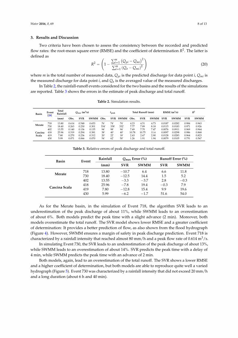
As for the Merate basin, in the simulation of Event 718, the algorithm SVR leads to anunderestimation of the peak discharge of about 11%, while SWMM leads to an overestimationof about 6%. Both models predict the peak time with a slight advance (2 min). Moreover, bothmodels overestimate the total runoff. The SVR model shows lower RMSE and a greater coefficientof determination: It provides a better prediction of flow, as also shown from the flood hydrograph(Figure 4). However, SWMM ensures a margin of safety in peak discharge prediction. Event 718 ischaracterized by a rainfall intensity that reached almost 80 mm/h and a peak flow rate of 0.614 m3/s.

In simulating Event 730, the SVR leads to an underestimation of the peak discharge of about 13%,while SWMM leads to an overestimation of about 14%. SVR predicts the peak time with a delay of4 min, while SWMM predicts the peak time with an advance of 2 min.

Both models, again, lead to an overestimation of the total runoff. The SVR shows a lower RMSEand a higher coefficient of determination, but both models are able to reproduce quite well a variedhydrograph (Figure 5). Event 730 was characterized by a rainfall intensity that did not exceed 20 mm/hand a long duration (about 6 h and 40 min).

Water 2016, 8, 69 9 of 13Water 2016, 8, 69 9 of 13

(a) (b)

(c) (d)

Figure 4. Simulation of the testing event 718 (Merate basin), (a) rainfall; (b) storm hydrograph; (c) predicted versus observed discharge (SVM); (d) predicted versus observed discharge (SWMM).

Both models, again, lead to an overestimation of the total runoff. The SVR shows a lower RMSE and a higher coefficient of determination, but both models are able to reproduce quite well a varied hydrograph (Figure 5). Event 730 was characterized by a rainfall intensity that did not exceed 20 mm/h and a long duration (about 6 h and 40 min).

(a) (b)

(c) (d)

Figure 5. Simulation of the testing event 730 (Merate basin). (a) Rainfall; (b) storm hydrograph; (c) predicted versus observed discharge (SVM); (d) predicted versus observed discharge (SWMM).

0

20

40

60

800.0 0.2 0.4 0.6 0.8 1.0

i [mm/hr]

t/tmax 0

0.2

0.4

0.6

0.8

0 0.2 0.4 0.6 0.8 1

Q [m3/s]

t/tmax

SVR

SWMM

Experimental data

0

0.2

0.4

0.6

0.8

0 0.2 0.4 0.6 0.8

QSVM [m3/s]

Qobs [m3/s]0

0.2

0.4

0.6

0.8

0 0.2 0.4 0.6 0.8

QSWMM[m3/s]

Qobs [m3/s]

0

5

10

15

200.0 0.2 0.4 0.6 0.8 1.0

i [mm/hr]

t/tmax0

0.1

0.2

0.3

0.4

0 0.2 0.4 0.6 0.8 1

Q [m3/s]

t/tmax

SVR

SWMM

Experimental data

0

0.1

0.2

0.3

0 0.1 0.2 0.3

QSVM [m3/s]

Qobs [m3/s]0

0.1

0.2

0.3

0 0.1 0.2 0.3

QSWMM[m3/s]

Qobs [m3/s]

Figure 4. Simulation of the testing event 718 (Merate basin), (a) rainfall; (b) storm hydrograph;(c) predicted versus observed discharge (SVM); (d) predicted versus observed discharge (SWMM).

Water 2016, 8, 69 9 of 13

(a) (b)

(c) (d)

Figure 4. Simulation of the testing event 718 (Merate basin), (a) rainfall; (b) storm hydrograph; (c) predicted versus observed discharge (SVM); (d) predicted versus observed discharge (SWMM).

Both models, again, lead to an overestimation of the total runoff. The SVR shows a lower RMSE and a higher coefficient of determination, but both models are able to reproduce quite well a varied hydrograph (Figure 5). Event 730 was characterized by a rainfall intensity that did not exceed 20 mm/h and a long duration (about 6 h and 40 min).

(a) (b)

(c) (d)

Figure 5. Simulation of the testing event 730 (Merate basin). (a) Rainfall; (b) storm hydrograph; (c) predicted versus observed discharge (SVM); (d) predicted versus observed discharge (SWMM).

0

20

40

60

800.0 0.2 0.4 0.6 0.8 1.0

i [mm/hr]

t/tmax 0

0.2

0.4

0.6

0.8

0 0.2 0.4 0.6 0.8 1

Q [m3/s]

t/tmax

SVR

SWMM

Experimental data

0

0.2

0.4

0.6

0.8

0 0.2 0.4 0.6 0.8

QSVM [m3/s]

Qobs [m3/s]0

0.2

0.4

0.6

0.8

0 0.2 0.4 0.6 0.8

QSWMM[m3/s]

Qobs [m3/s]

0

5

10

15

200.0 0.2 0.4 0.6 0.8 1.0

i [mm/hr]

t/tmax0

0.1

0.2

0.3

0.4

0 0.2 0.4 0.6 0.8 1

Q [m3/s]

t/tmax

SVR

SWMM

Experimental data

0

0.1

0.2

0.3

0 0.1 0.2 0.3

QSVM [m3/s]

Qobs [m3/s]0

0.1

0.2

0.3

0 0.1 0.2 0.3

QSWMM[m3/s]

Qobs [m3/s]

Figure 5. Simulation of the testing event 730 (Merate basin). (a) Rainfall; (b) storm hydrograph;(c) predicted versus observed discharge (SVM); (d) predicted versus observed discharge (SWMM).

Regarding the Cascina Scala basin, in the simulation of Event 402, both models provide a slightunderestimation of the peak discharge (the error is 3.3% for SVR and 3.7% for SWMM). The peak time

Water 2016, 8, 69 10 of 13

is predicted with a delay of 4 min by SVR, while it is predicted with great accuracy by SWMM. Even thetotal runoff is well predicted by SWMM, while SVR leads to a slight overestimation. Once again, SVRpredictions are characterized by lower RMSE and a greater coefficient of determination. Additionally, inthis case both models can reproduce the flood hydrograph quite well (Figure 6), except at the beginning,where the SVR algorithm unreasonably provides flow rates other than zero.

Water 2016, 8, 69 10 of 13

Regarding the Cascina Scala basin, in the simulation of Event 402, both models provide a slight underestimation of the peak discharge (the error is 3.3% for SVR and 3.7% for SWMM). The peak time is predicted with a delay of 4 min by SVR, while it is predicted with great accuracy by SWMM. Even the total runoff is well predicted by SWMM, while SVR leads to a slight overestimation. Once again, SVR predictions are characterized by lower RMSE and a greater coefficient of determination. Additionally, in this case both models can reproduce the flood hydrograph quite well (Figure 6), except at the beginning, where the SVR algorithm unreasonably provides flow rates other than zero.

(a) (b)

(c) (d)

Figure 6. Simulation of the testing event 402 (Cascina Scala basin), (a) rainfall; (b) storm hydrograph; (c) predicted versus observed discharge (SVM); (d) predicted versus observed discharge (SWMM).

As for Event 418, SVR leads to an underestimation of the peak discharge of 7.8%, while the SWMM model provides an overestimation of almost 20%. Both models forecast the peak time with a delay of 2 min. The SVR algorithm well predicts the total runoff, while SWMM leads to a slight overestimation. The better accuracy of SVR is certified also in this case by RMSE and CE.

In simulating Event 419 SVR provides an appreciable underestimation of the peak flow rate (−12.8%), while SWMM provides a somewhat higher result than the experimental one (+15.4%). The peak time is predicted with a delay of 2 min by SVR, while it is predicted with an advance of 2 min by SWMM. Both models provide a considerable overestimation of the total runoff (+9.9% SVR, +19.6% SWMM), while SVR shows lower RMSE and a greater coefficient of determination.

Finally, in simulating Event 430 both models produce less satisfactory results than in the other events.

0

2

4

6

8

10

120.0 0.2 0.4 0.6 0.8 1.0

i [mm/hr]

t/tmax0

0.04

0.08

0.12

0.16

0 0.2 0.4 0.6 0.8 1

Q [m3/s]

t/tmax

SVR

SWMM

Experimental data

0

0.05

0.1

0.15

0.2

0 0.05 0.1 0.15 0.2

QSVM [m3/s]

Qobs [m3/s]0

0.05

0.1

0.15

0.2

0 0.05 0.1 0.15 0.2

QSWMM [m3/s]

Qobs [m3/s]

Figure 6. Simulation of the testing event 402 (Cascina Scala basin), (a) rainfall; (b) storm hydrograph;(c) predicted versus observed discharge (SVM); (d) predicted versus observed discharge (SWMM).

As for Event 418, SVR leads to an underestimation of the peak discharge of 7.8%, while theSWMM model provides an overestimation of almost 20%. Both models forecast the peak time witha delay of 2 min. The SVR algorithm well predicts the total runoff, while SWMM leads to a slightoverestimation. The better accuracy of SVR is certified also in this case by RMSE and CE.

In simulating Event 419 SVR provides an appreciable underestimation of the peak flow rate(´12.8%), while SWMM provides a somewhat higher result than the experimental one (+15.4%).The peak time is predicted with a delay of 2 min by SVR, while it is predicted with an advance of 2 minby SWMM. Both models provide a considerable overestimation of the total runoff (+9.9% SVR, +19.6%SWMM), while SVR shows lower RMSE and a greater coefficient of determination.

Finally, in simulating Event 430 both models produce less satisfactory results than in theother events.

Even if the errors on the peak flow rate and on time to peak are small, the error on the total runoffexceeds 50% for both SVR and SWMM. Both models fail to adequately simulate the second part ofthe hydrograph (Figure 7). Obviously, the RMSE and the coefficient of determination certify in a clearmanner the smaller accuracy of the results. The reason why both models show poor performance inthis case is not easy to understand. Probably the hyetograph, which is significantly different from thoseused in the calibration procedures, is the main cause of the unsatisfactory results. In this hyetograph,the highest rainfall intensity is observed for t/tmax < 0.2. For t/tmax > 0.2 rainfall intensity is reduced,except for a short time interval around t/tmax = 0.5. None of the events that have been considered in

Water 2016, 8, 69 11 of 13

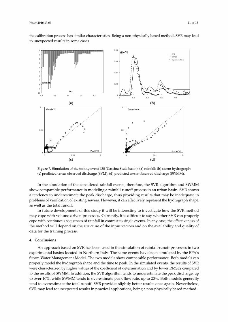
the calibration process has similar characteristics. Being a non-physically based method, SVR may leadto unexpected results in some cases.Water 2016, 8, 69 11 of 13

(a) (b)

(c) (d)

Figure 7. Simulation of the testing event 430 (Cascina Scala basin), (a) rainfall; (b) storm hydrograph; (c) predicted versus observed discharge (SVM); (d) predicted versus observed discharge (SWMM).

Even if the errors on the peak flow rate and on time to peak are small, the error on the total runoff exceeds 50% for both SVR and SWMM. Both models fail to adequately simulate the second part of the hydrograph (Figure 7). Obviously, the RMSE and the coefficient of determination certify in a clear manner the smaller accuracy of the results. The reason why both models show poor performance in this case is not easy to understand. Probably the hyetograph, which is significantly different from those used in the calibration procedures, is the main cause of the unsatisfactory results. In this hyetograph, the highest rainfall intensity is observed for t/tmax < 0.2. For t/tmax > 0.2 rainfall intensity is reduced, except for a short time interval around t/tmax = 0.5. None of the events that have been considered in the calibration process has similar characteristics. Being a non-physically based method, SVR may lead to unexpected results in some cases.

In the simulation of the considered rainfall events, therefore, the SVR algorithm and SWMM show comparable performance in modeling a rainfall-runoff process in an urban basin. SVR shows a tendency to underestimate the peak discharge, thus providing results that may be inadequate in problems of verification of existing sewers. However, it can effectively represent the hydrograph shape, as well as the total runoff.

In future developments of this study it will be interesting to investigate how the SVR method may cope with volume driven processes. Currently, it is difficult to say whether SVR can properly cope with continuous sequences of rainfall in contrast to single events. In any case, the effectiveness of the method will depend on the structure of the input vectors and on the availability and quality of data for the training process.

4. Conclusions

An approach based on SVR has been used in the simulation of rainfall-runoff processes in two experimental basins located in Northern Italy. The same events have been simulated by the EPA’s Storm Water Management Model. The two models show comparable performance. Both models can properly model the hydrograph shape and the time to peak. In the simulated events, the results of SVR were characterized by higher values of the coefficient of determination and by lower RMSEs

0

1

2

3

4

5

6

7

8

9

100.0 0.2 0.4 0.6 0.8

i [mm/hr]

t/tmax0

0.02

0.04

0.06

0.08

0 0.2 0.4 0.6 0.8 1

Q [m3/s]

t/tmax

SVR

SWMM

Experimental data

0

0.05

0.1

0 0.05 0.1

QSVM [m3/s]

Qobs[m3/s]0

0.05

0.1

0 0.05 0.1

QSWMM [m3/s]

Qobs [m3/s]

Figure 7. Simulation of the testing event 430 (Cascina Scala basin), (a) rainfall; (b) storm hydrograph;(c) predicted versus observed discharge (SVM); (d) predicted versus observed discharge (SWMM).

In the simulation of the considered rainfall events, therefore, the SVR algorithm and SWMMshow comparable performance in modeling a rainfall-runoff process in an urban basin. SVR showsa tendency to underestimate the peak discharge, thus providing results that may be inadequate inproblems of verification of existing sewers. However, it can effectively represent the hydrograph shape,as well as the total runoff.

In future developments of this study it will be interesting to investigate how the SVR methodmay cope with volume driven processes. Currently, it is difficult to say whether SVR can properlycope with continuous sequences of rainfall in contrast to single events. In any case, the effectiveness ofthe method will depend on the structure of the input vectors and on the availability and quality ofdata for the training process.

4. Conclusions

An approach based on SVR has been used in the simulation of rainfall-runoff processes in twoexperimental basins located in Northern Italy. The same events have been simulated by the EPA’sStorm Water Management Model. The two models show comparable performance. Both models canproperly model the hydrograph shape and the time to peak. In the simulated events, the results of SVRwere characterized by higher values of the coefficient of determination and by lower RMSEs comparedto the results of SWMM. In addition, the SVR algorithm tends to underestimate the peak discharge, upto over 10%, while SWMM tends to overestimate peak flow rate, up to 20%. Both models generallytend to overestimate the total runoff: SVR provides slightly better results once again. Nevertheless,SVR may lead to unexpected results in practical applications, being a non-physically based method.

Water 2016, 8, 69 12 of 13

SVR shows considerable potential for applications to the problems of urban hydrology. However,it is necessary to work hard to overcome the current limitations of this approach. It is essential totry to automate the identification of a suitable kernel function and of the main features of the model.Therefore, it appears appropriate that a similar approach is tested on a large number of case studies.

Author Contributions: Francesco Granata conceived this research, performed data collection, developed themodels and carried out the model simulations. All the authors analyzed the results, wrote and approvedthe manuscript.

Conflicts of Interest: The authors declare no conflict of interest.

References

1. Butler, D.; Davies, J. Urban Drainage, 3rd ed.; CRC Press: Boca Raton, FL, USA, 2011.2. Coombes, P.J. Transitioning Drainage into Urban Water Cycle Management. In Proceedings of the WSUD2015

Conference, Engineers Australia, Sydney, Australia, 2015.3. Beven, K.J. Rainfall-Runoff Modelling: The Primer, 2nd ed.; Wiley-Blackwell: Oxford, UK, 2012.4. Coombes, P.J.; Babister, M.; McAlister, T. Is the Science and Data underpinning the Rational Method

Robust for use in Evolving Urban Catchments. In Proceedings of the 36th Hydrology and Water ResourcesSymposium, Engineers Australia, Hobart, Australia, 2015.

5. ASCE Task Committee on Application of Artificial Neural Networks in Hydrology. Artificial NeuralNetworks in Hydrology. I: Preliminary Concepts. J. Hydrol. Eng. 2000, 5, 115–123.

6. ASCE Task Committee on Application of Artificial Neural Networks in Hydrology Artificial NeuralNetworks in Hydrology. II: Hydrologic Applications. J. Hydrol. Eng. 2000, 5, 124–137.

7. Cristianini, N.; Shawe-Taylor, J. An Introduction to Support Vector Machines; Cambridge University Press:Cambridge, UK, 2000.

8. Vapnik, V. The Nature of Statistical Learning Theory; Springer: New York, NY, USA, 1995.9. Cortes, C.; Vapnik, V. Support vector networks. Mach. Learn. 1995, 20, 273–297. [CrossRef]10. Boser, B.E.; Guyon, I.M.; Vapnik, V.N. A training algorithm for optimal margin classifiers. In Proceedings of

the Annual Conference on Computational Learning Theory, Pittsburgh, PA, USA; ACM Press: New York,NY, USA, 1992; pp. 144–152.

11. Vapnik, V.; Golowich, S.; Smola, A. Support vector method for function approximation, regression estimation,and signal processing. In Advances in Neural Information Processing Systems; Mozer, M.C., Jordan, M.I.,Petsche, T., Eds.; MIT Press: Cambridge, MA, USA, 1997; pp. 281–287.

12. Dibike, Y.B.; Velickov, S.; Solomatine, D.; Abbott, M.B. Model induction with sup-port vector machines:Introduction and application. J. Comput. Civil Eng. 2001, 15, 208–216. [CrossRef]

13. Bray, M.; Han, D. Identification of support vector machines for runoff modelling. J. Hydroinf. 2004, 6, 265–280.14. Tripathi, S.H.; Srinivas, V.V.; Nanjundiah, R.S. Downscaling of precipitation for climate change scenarios: A

support vector machine approach. J. Hydrol. 2006, 330, 621–640. [CrossRef]15. Chen, H.; Guo, J.; Wei, X. Downscaling GCMs using the smooth support vector machine method to predict

daily precipitation in the Hanjiang basin. Adv. Atmos. Sci. 2010, 27, 274–284. [CrossRef]16. Garcìa Nieto, P.J.; Martinez Torres, J.; Araùjo Fernàndez, M.; Ordònez Galàn, C. Support vector machines

and neural networks used to evaluate paper manufactured using Eucalyptus globulus. Appl. Math. Model.2012, 36, 6137–6145. [CrossRef]

17. Antonanzas, J.; Urraca, R.; Martinez-de-Pison, F.J.; Antonanzas-Torres, F. Solar irradiation mapping withexogenous data from support vector regression machines estimations. Energy Convers. Manag. 2015, 100,380–390. [CrossRef]

18. Yu, P.S.; Chen, S.T.; Chang, I.F. Support vector regression for real-time flood stage forecasting. J. Hydrol. 2006,328, 704–716. [CrossRef]

19. Hosseini, S.M.; Mahjouri, N. Integrating Support Vector Regression and a geomorphologic Artificial NeuralNetwork for daily rainfall-runoff modeling. Appl. Soft Comput. 2016, 38, 329–345. [CrossRef]

20. Raghavendra, S.N.; Deka, P.C. Support vector machine applications in the field of hydrology: A review.Appl. Soft Comput. 2014, 19, 372–386. [CrossRef]

Water 2016, 8, 69 13 of 13

21. Chang, C.C.; Lin, C.J. Training ν-support vector classifiers: Theory and algorithms. Neural Comput. 2001, 13,2119–2147. [CrossRef] [PubMed]

22. Smola, A.J.; Scholkopf, B. A tutorial on support vector regression. Stat. Comput. 2004, 14, 199–222. [CrossRef]23. Karush, W. Minima of functions of several variables with inequalities as side constraints. Master’s Thesis,

Department of Mathematics, University of Chicago, Chicago, IL, USA, 1939.24. Kuhn, H.W.; Tucker, A.W. Nonlinear programming. In Proceedings of the 2nd Berkeley Symposium

on Mathematical Statistics and Probabilistics; University of California Press: Oakland, CA, USA, 1951;pp. 481–492.

25. Rossman, L.A. Storm Water Management Model User’s Manual, Version 5.0; U.S. Environmental ProtectionAgency: Cincinnati, OH, USA, 2004.

26. Box, M.J. A new method of constrained optimization and comparison with other methods. Comput. J. 1965,8, 42–52. [CrossRef]

27. Barco, J.; Wong, K.M.; Stenstrom, M.K. Automatic Calibration of the U.S. EPA SWMM Model for a LargeUrban Catchment. J. Hydraul. Eng. 2008, 134, 466–474. [CrossRef]

28. Calomino, F.; Paoletti, A. Le Misure di Pioggia e di Portata Nei Bacini Sperimentali Urbani in Italia; CSDU: Milan,Italy, 1994.

© 2016 by the authors; licensee MDPI, Basel, Switzerland. This article is an open accessarticle distributed under the terms and conditions of the Creative Commons by Attribution(CC-BY) license (http://creativecommons.org/licenses/by/4.0/).