Supply shocks, demand shocks, and labor market fluctuations

Research Division Federal Reserve Bank of St. Louis Working Paper Series

Supply Shocks, Demand Shocks, and Labor Market Fluctuations

Helge Braun Reinout De Bock

and Riccardo DiCecio

Working Paper 2007-015A http://research.stlouisfed.org/wp/2007/2007-015.pdf

April 2007

FEDERAL RESERVE BANK OF ST. LOUIS Research Division

P.O. Box 442 St. Louis, MO 63166

______________________________________________________________________________________

The views expressed are those of the individual authors and do not necessarily reflect official positions of the Federal Reserve Bank of St. Louis, the Federal Reserve System, or the Board of Governors.

Federal Reserve Bank of St. Louis Working Papers are preliminary materials circulated to stimulate discussion and critical comment. References in publications to Federal Reserve Bank of St. Louis Working Papers (other than an acknowledgment that the writer has had access to unpublished material) should be cleared with the author or authors.

Supply Shocks, Demand Shocks, and LaborMarket Fluctuations�

Helge BraunUniversity of British Columbia

Reinout De BockNorthwestern University

Riccardo DiCecioFederal Reserve Bank of St. Louis

April 2007

Abstract

We use structural vector autoregressions to analyze the responses of worker�ows, job �ows, vacancies, and hours to shocks. We identify demand and sup-ply shocks by restricting the short-run responses of output and the price level.On the demand side we disentangle a monetary and non-monetary shock byrestricting the response of the interest rate. The responses of labor market vari-ables are similar across shocks: expansionary shocks increase job creation, thehiring rate, vacancies, and hours. They decrease job destruction and the sep-aration rate. Supply shocks have more persistent e¤ects than demand shocks.Demand and supply shocks are equally important in driving business cycle �uc-tuations of labor market variables. Our �ndings for demand shocks are robustto alternative identi�cation schemes involving the response of labor productiv-ity at di¤erent horizons and an alternative speci�cation of the VAR. However,supply shocks identi�ed by restricting productivity generate a higher fractionof responses inconsistent with standard search and matching models.JEL: C32, E24, E32, J63.Keywords: business cycles, job �ows, unemployment, vacancies, vector au-

toregressions, worker �ows.

�We are grateful to Paul Beaudry, Larry Christiano, Martin Eichenbaum, Luca Dedola, DanielLevy, Éva Nagypál, Dale Mortensen, Frank Smets and seminar participants at the ECB, 2006Midwest Macroeconomics Meetings, and WEAI 81st Annual Conference for helpful comments. Wethank Steven Davis, and Robert Shimer for sharing their data. Helge Braun and Reinout De Bockthank the research department at the St. Louis FRB and the ECB, respectively, for their hospitality.Reinout De Bock gratefully acknowledges �nancial support from the University of Antwerp. Anyviews expressed are our own and do not necessarily re�ect the views of the Federal Reserve Bank ofSt. Louis or the Federal Reserve System. All errors are our own. Corresponding author: RiccardoDiCecio, [email protected]

1

1 Introduction

Hall (2005) and Shimer (2004) argue that the Mortensen-Pissarides matching model(Mortensen and Pissarides, 1994) is unable to reproduce the volatility of the job-�nding rate, unemployment, and vacancies observed in the data. A growing literaturehas attempted to augment the basic Mortensen-Pissarides model in order to matchthese business cycle facts.1 Although most of this literature considers shocks to laborproductivity as the source of �uctuations, some authors invoke the responses to othershocks as a potential resolution (see Silva and Toledo, 2005). These analyses arebased on the assumption that either the unconditional moments are driven to a largeextent by a particular shock, or the responses of the labor market to di¤erent shocksare similar. In this paper, we take a step back and ask what the contributions ofdi¤erent aggregate shocks to labor market �uctuations are and to what extent thelabor market responds di¤erentially to shocks. The labor market variables we analyzeare worker �ows, job �ows, vacancies, and hours. Including both worker and job �owsallows us to analyze the di¤erent conclusions authors have reached with respect to theimportance of the hiring versus separation margin in driving changes in employmentand unemployment. Including aggregate hours relates our work to the literature onthe response of hours to technology shocks.We identify three aggregate shocks �supply shocks, monetary, and non-monetary

demand shocks �using a structural vector autoregression. We place restrictions on thesigns of the dynamic responses of aggregate variables as in Uhlig (2005) and Peersman(2005). The �rst identi�cation scheme we consider places restrictions on the short-runresponses of output, the price level, and the interest rate. We require that supplyshocks move output and the price level in opposite directions, while demand shocksgenerate price and output responses of the same sign. Monetary shocks additionallylower the interest rate on impact; other demand shocks do not. These restrictionsare motivated by a basic IS-LM-AD-AS framework or by new-Keynesian models. Weleave the responses of job �ows, worker �ows, hours and vacancies unrestricted.The main results for the labor market variables are as follows: The responses of

hours, job �ows, worker �ows, and vacancies are at least qualitatively similar acrossshocks. A positive demand or supply shock increases vacancies, the job-�nding andcreation rates, and decreases the separation and job-destruction rates. As in Fujita(2004), the responses of vacancies and the job-�nding rate are persistent and humpshaped. Furthermore, the responses induced by demand shocks are less persistentthan those induced by supply shocks. Across shocks, changes in the job-�ndingrate are responsible for the bulk of changes in unemployment, although separationscontribute up to one half on impact. Changes in employment, on the other had, aremostly driven by the job destruction rate. As in Davis and Haltiwanger (1999), we�nd that job reallocation falls following expansionary shocks, especially for demand-side shocks. We �nd no evidence of di¤erences in the matching process of unemployedworkers and vacancies in response to di¤erent shocks. Finally, each of the demandside-shocks is at least as important as the supply side shock in explaining �uctuations

1See, for example, Hagedorn and Manovskii (2006) and Mortensen and Nagypal (2005).

2

in labor market variables.There is mild evidence in support of a technological interpretation of the supply

shocks identi�ed by these restrictions. The response of labor productivity is positivefor supply shocks at medium-term horizons, whereas insigni�cantly di¤erent fromzero for the demand shocks. To check the robustness of our results, we modify ouridenti�cation scheme by restricting the medium-run response of labor productivity toidentify the supply-side shock, while leaving the short-run responses of output andthe price level unrestricted. This identi�cation scheme is akin to a long-run restrictionon the response of labor productivity used in the literature. Consistent with the �rstidenti�cation scheme, technology shocks tend to raise output and decrease the pricelevel in the short run.Interestingly, the labor market responses to supply shocks under this identi�cation

scheme are less clear cut. In particular, the responses of vacancies, worker and job�ows to supply shocks are not signi�cantly di¤erent from zero. Again, the demandside shocks are at least as important in explaining �uctuations in the labor marketvariables as the supply shock. We also identify a technology shock, using a long-run restriction on labor productivity, and a monetary shock, via the recursivenessassumption used by Christiano, Eichenbaum, and Evans (1999). Again, we �nd thatthe responses to the technology shock are not signi�cantly di¤erent from zero. Theresponses to the monetary shock are consistent with the ones identi�ed above. Thecontribution of the monetary shock to the variance of labor-market variables exceedsthat of the technology shock.We also analyze the subsample stability of our results. We �nd a reduction in the

volatility of shocks, consistent with the Great Moderation literature, for the post-1984subsample. The main conclusions from the analysis above apply to both subsamples.Furthermore, we use a small VAR including only non-labor market variables and

hours to identify the shocks. We then uncover the responses of the labor marketvariables by regressing them on distributed lags of the shocks. Our �ndings arerobust to this alternative empirical strategy.Our results suggest that a reconciliation of the Mortensen-Pissarides model should

equally apply to the response of labor market variables to demand side shocks. Fur-thermore, the response to supply side shocks is much less clear cut than implicitlyassumed in the bulk of the literature. In a related paper, Braun, De Bock, and DiCe-cio (2006) further explore the labor market responses to di¤erentiated supply shocks(see also Lopez-Salido and Michelacci, 2005).Also, our �ndings suggest that the �hours debate� spawned by Galì (1999) is

relevant for business cycle models with a Mortensen-Pissarides labor market. In tryingto uncover the source of business cycle �uctuations, several authors have argued thata negative response of hours worked to supply shocks is inconsistent with the standardreal business cycle (RBC) model. These results are often interpreted as suggestingthat demand-side shocks must play an important role in driving the cycle and usedas empirical support for models that depart from the RBC standard by incorporatingnominal rigidities and other frictions. We provide empirical evidence on the responseof job �ows, worker �ows, and vacancies. This is a necessary step to evaluate theempirical soundness of business cycle models with a labor market structure richer

3

than the competitive structure typical of the RBC models or the stylized sticky-wages structure often adopted in new-Keynesian models. The importance of demandshocks in driving labor-market variables and the atypical responses to supply shockscan be interpreted as a milder version of the �negative response of hours��ndings.The paper is organized as follows. Section 2 describes the data used in the analysis.

Section 3 describes the identi�cation procedure. Results are presented and discussedin Section 4. Section 5 contains the robustness analysis. Section 6 concludes.

2 Worker Flows and Job Flows Data

For worker �ows data, we use the separation and job-�nding rates constructed byShimer (2005b). We brie�y discuss their construction in Section 2.1. For job �owsdata, we take the job creation and destruction series recently constructed by Faber-man (2004) and Davis, Faberman, and Haltiwanger (2005), as discussed in Section2.2. Section 2.3 presents business cycle statistics of the data.

2.1 Separation and Job-Finding Rates

The separation rate measures the rate at which workers leave employment and enterthe unemployment pool. The job-�nding rate measures the rate at which unemployedworkers exit the unemployment pool. Although the rates are constructed and inter-preted while omitting �ows between labor market participation and non-participation,Shimer (2005b) shows that they capture the most important cyclical determinants ofthe behavior of both the unemployment and employment pools over the business cy-cle. The advantage of using these data lies in its availability for a long time span. Thedata constructed by Shimer are available from 1947, whereas worker �ow data includ-ing non-participation �ows from the Current Population Survey (CPS) are availableonly from 1967 onward.The separation and job-�nding rates are constructed using data on the short-

term unemployment rate as a measure of separations and the law of motion for theunemployment rate to back out a measure of the job-�nding rate. The size of theunemployment pool is observed at discrete dates t; t + 1; t + 2:::. Hirings and sepa-rations occur continuously between these dates. To identify the relevant rates withina time period, assume that between dates t and t + 1, separations and job-�ndingoccur with constant Poisson arrival rates st and ft, respectively: For some � 2 (0; 1),the law of motion for the unemployment pool Ut+� is

�U t+� = Et+�st � Ut+�ft;

where Et+� is the pool of employed workers. Here, Et+�st are simply the in�ows andUt+�ft the out�ows from the unemployment pool at t+ � . The analogous expressionfor the pool of short-term unemployed U st+� (i.e., those workers who have entered theunemployment pool after date t) is:

�Us

t+� = Et+�st � U st+�ft:

4

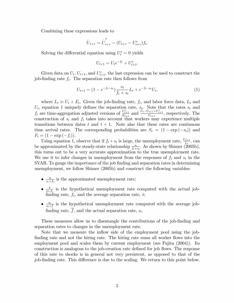
Combining these expressions leads to

�U t+� =

�Us

t+� � (Ut+� � U st+� )ft:

Solving the di¤erential equation using U st = 0 yields

Ut+1 = Ute�ft + U st+1:

Given data on Ut; Ut+1, and U st+1, the last expression can be used to construct thejob-�nding rate ft. The separation rate then follows from

Ut+1 = (1� e�ft�st)st

ft + stLt + e

�ft�stUt; (1)

where Lt � Ut + Et. Given the job-�nding rate, ft, and labor force data, Lt andUt, equation 1 uniquely de�nes the separation rate, st. Note that the rates st andft are time-aggregation adjusted versions of

Ust+1Et+1

andUt�Ut+1+Ust+1

Ut+1, respectively. The

construction of st and ft takes into account that workers may experience multipletransitions between dates t and t + 1. Note also that these rates are continuoustime arrival rates. The corresponding probabilities are St = (1� exp (�st)) andFt = (1� exp (�ft)).Using equation 1, observe that if ft+st is large, the unemployment rate,

Ut+1Lt; can

be approximated by the steady-state relationship stft+st

: As shown by Shimer (2005b),this turns out to be a very accurate approximation to the true unemployment rate.We use it to infer changes in unemployment from the responses of ft and st in theSVAR. To gauge the importance of the job �nding and separation rates in determiningunemployment, we follow Shimer (2005b) and construct the following variables:

� stst+ft

is the approximated unemployment rate;

� �s�s+ft

is the hypothetical unemployment rate computed with the actual job-�nding rate, ft, and the average separation rate, �s;

� stst+ �f

is the hypothetical unemployment rate computed with the average job-

�nding rate, f , and the actual separation rate, st:

These measures allow us to disentangle the contributions of the job-�nding andseparation rates to changes in the unemployment rate.Note that we measure the in�ow side of the employment pool using the job-

�nding rate and not the hiring rate. The hiring rate sums all worker �ows into theemployment pool and scales them by current employment (see Fujita (2004)). Itsconstruction is analogous to the job-creation rate de�ned for job �ows. The responseof this rate to shocks is in general not very persistent, as opposed to that of thejob-�nding rate. This di¤erence is due to the scaling. We return to this point below.

5

2.2 Job Creation and Job Destruction

The job �ows literature focuses on job-creation (JC) and destruction (JD) rates.2

Gross job creation sums up employment gains at all plants that expand or start upbetween t� 1 and t. Gross job destruction, on the other hand, sums up employmentlosses at all plants that contract or shut down between t � 1 and t. To obtainthe creation and destruction rates, both measures are divided by the averages ofemployment at t�1 and t. Davis, Haltiwanger, and Schuh (1996) constructed measuresfor both series from the Longitudinal Research Database (LRD) and the monthlyCurrent Employment Statistics (CES) survey from the Bureau of Labor Statistics(BLS).3 A number of researchers work only with the quarterly job creation and jobdestruction series from the LRD.4 Unfortunately this series is available only for the1972:Q1-1993:Q4 period.In this paper we work with the quarterly job �ows constructed by Faberman

(2004), and Davis, Faberman, and Haltiwanger (2005) from three sources. Theseauthors splice together data from the (i) BLS manufacturing Turnover Survey (MTD)from 1947 to 1982, (ii) the LRD from 1972 to 1998, and (iii) the Business EmploymentDynamics (BED) from 1990 to 2004. The MTD-LRD data are spliced as in Davisand Haltiwanger (1999), whereas the LRD-BED splice follows Faberman (2004).A fundamental accounting identity relates the net employment change between

any two points in time to the di¤erence between job creation and destruction. Wede�ne gJC;JDE;t as the growth rate of employment implied by job �ows:

gJC;JDE;t � Et � Et�1(Et + Et�1) =2

� JCt � JDt. (2)

The data spliced from the MTD and LRD of the job-creation and -destructionrates constructed by Davis, Faberman, and Haltiwanger (2005) pertain to the manu-facturing sector. However, over the period 1954:Q2-2004:Q2, the implied growth rateof employment from these job �ows data, gJC;JDE;t � (JCt � JDt), is highly correlated

with the growth rate of total non-farm payroll employment, gE;t �h

Et�Et�10:5(Et+Et�1)

i:

Corr�gJC;JDE;t ; gE;t

�= 0:89.5

As in Davis, Haltiwanger, and Schuh (1996), we also de�ne gross job reallocationrt as

rt � JCt + JDt: (3)

2See Davis and Haltiwanger (1992), Davis, Haltiwanger, and Schuh (1996), Davis and Haltiwanger(1999), Caballero and Hammour (2005), and Lopez-Salido and Michelacci (2005).

3As pointed out in Blanchard and Diamond (1990) these job creation and destruction measuresdi¤er from true job creation and destruction as (i) they ignore gross job creation and destructionwithin �rms, (ii) the point-in-time observations do not take into account job creation and destructiono¤sets within the quarter, and (iii) they fail to account for newly created jobs that are not �lledwith workers yet.

4Davis and Haltiwanger (1999) extend the series back to 1948. Some authors report that thisextended series is (i) somewhat less accurate and (ii) only tracks aggregate employment in the1972:Q1-1993:Q4 period (see Caballero and Hammour (2005)).

5The correlation of gJC;JDE;t with the growth rate of employment in manufacturing is 0:93.

6

Using this de�nition we examine the reallocation e¤ects of a particular shock inthe SVARs. We also look at cumulative reallocation.

2.3 Business Cycle Properties

Table 1 reports correlations and standard deviations (relative to output) for the busi-ness cycle component6 of worker �ows, job �ows, the unemployment rate (u), vacan-cies (v), and output (y).7 The job-�nding rate and vacancies are strongly procyclical.Job creation is moderately procyclical. The separation rate, job destruction and theunemployment rate are countercyclical. Job destruction is one-and-a-half times morevolatile than job creation. The job-�nding rate is twice as volatile as the separationrate. Notice that job destruction and the separation rate are positively correlated,whereas job creation and the job-�nding rate are orthogonal to each other.In Table 2 we report correlations of the three unemployment approximations de-

scribed in Section 2.1 with actual unemployment, and standard deviations (relativeto actual unemployment). The steady-state approximation to unemployment is veryaccurate, and the job-�nding rate plays a bigger role in determining unemployment.The contribution of the job-�nding rate is even larger at cyclical frequencies.8

3 Structural VAR Analysis

In this section, we describe the reduced-form VAR speci�cation and provide an out-line of the Bayesian implementation of sign restrictions. The variables included inthe SVAR analysis are the growth rate of average labor productivity (� lnY=H), thein�ation rate (� ln p), hours (lnH), worker �ows (job-�nding and separation rates),job �ows (job creation and destruction), a measure of vacancies (ln v), and the fed-eral funds rate (ln (1 +R)). Worker �ows are the job-�nding and separation ratesconstructed in Shimer (2005b). Job �ows are the job-creation and destruction seriesfrom Faberman (2004) and Davis, Faberman, and Haltiwanger (2005). Sources for theother data are given in Appendix A. The sample covers the period 1954:Q2-2004:Q2.The variables are required to be covariance stationary. To achieve stationarity, welinearly detrend the logarithms of the job �ows variables. The estimated VAR coef-�cients corroborate the stationarity assumption.Consider the following reduced-form VAR:9

Zt = �+Pp

j=1BjZt�j + ut; Eutu0t = V; (4)

6We used the band-pass �lter described in Christiano and Fitzgerald (2003) for frequencies be-tween 8 and 32 quarters to extract the business-cycle component of the data.

7See Appendix A for data sources.8Shimer (2005a) uses an HP �lter with smoothing parameter 105. His choice of an unusual �lter

to detrend the data further magni�es the contribution of the job-�nding rate to unemployment withrespect to the �gures we report.

9Based on information criteria, we estimate a reduced form VAR including 2 lags, i.e., p = 2.

7

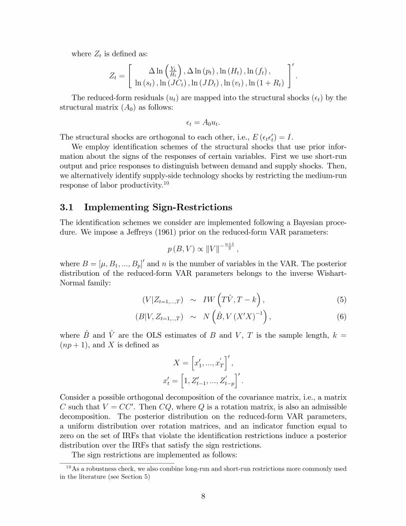
where Zt is de�ned as:

Zt =

"� ln

�YtHt

�;� ln (pt) ; ln (Ht) ; ln (ft) ;

ln (st) ; ln (JCt) ; ln (JDt) ; ln (vt) ; ln (1 +Rt)

#0:

The reduced-form residuals (ut) are mapped into the structural shocks (�t) by thestructural matrix (A0) as follows:

�t = A0ut:

The structural shocks are orthogonal to each other, i.e., E (�t�0t) = I.We employ identi�cation schemes of the structural shocks that use prior infor-

mation about the signs of the responses of certain variables. First we use short-runoutput and price responses to distinguish between demand and supply shocks. Then,we alternatively identify supply-side technology shocks by restricting the medium-runresponse of labor productivity.10

3.1 Implementing Sign-Restrictions

The identi�cation schemes we consider are implemented following a Bayesian proce-dure. We impose a Je¤reys (1961) prior on the reduced-form VAR parameters:

p (B; V ) / kV k�n+12 ;

where B = [�;B1; :::; Bp]0 and n is the number of variables in the VAR. The posterior

distribution of the reduced-form VAR parameters belongs to the inverse Wishart-Normal family:

(V jZt=1;:::;T ) � IW�T V̂ ; T � k

�; (5)

(BjV; Zt=1;::;T ) � N�B̂; V (X 0X)

�1�; (6)

where B̂ and V̂ are the OLS estimates of B and V , T is the sample length, k =(np+ 1), and X is de�ned as

X =hx01; :::; x

0

T

i0;

x0t =h1; Z 0t�1; :::; Z

0

t�p

i0:

Consider a possible orthogonal decomposition of the covariance matrix, i.e., a matrixC such that V = CC 0. Then CQ, where Q is a rotation matrix, is also an admissibledecomposition. The posterior distribution on the reduced-form VAR parameters,a uniform distribution over rotation matrices, and an indicator function equal tozero on the set of IRFs that violate the identi�cation restrictions induce a posteriordistribution over the IRFs that satisfy the sign restrictions.The sign restrictions are implemented as follows:

10As a robustness check, we also combine long-run and short-run restrictions more commonly usedin the literature (see Section 5)

8

1. For each draw from the inverse Wishart-Normal family for (V;B) in (5) and (6)we take an orthogonal decomposition matrix, C, and draw one possible rotation,Q.11

2. We check the signs of the impulse responses for each structural shock. If we�nd a set of structural shocks that satisfy the restrictions, we keep the draw.Otherwise we discard it.

3. We continue until we have 1,000 draws from the posterior distribution of theIRFs that satisfy the identifying restrictions.

4 Price and Output Restrictions

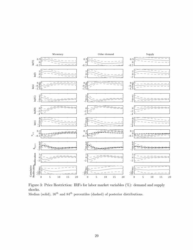
The basic IS-LM-AD-AS model can be used to motivate the following restrictionsto distinguish demand and supply shocks. Demand shocks move the price level andoutput in the same direction in the short run. Supply shocks, on the other hand, moveoutput and the price level in opposite directions. On the demand side, we furtherdistinguish between monetary and non-monetary shocks: Monetary shocks lower theinterest rate on impact whereas non-monetary demand shocks do not. The pricelevel and interest rate responses are restricted for one quarter, the output responseis restricted for four quarters. These restrictions are similar to the ones used byPeersman (2005).12 The identifying restrictions are summarized in Table 3.Figures 2 and 3 report the median, 16th, and 84th percentiles of 1,000 draws

from the posterior distribution of acceptable IRFs to the structural shocks of non-labor market variables, labor market variables, and other variables of interest. Recallthat labor market variables are left unrestricted. Note that the response of output ishump-shaped across shocks and more persistent for supply shocks. Furthermore, theresponse of hours is positive for all shocks and the response of labor productivity ispositive for supply shocks.For the response of the labor market variables displayed in Figure 3, the following

main observations emerge:

Similarity Across Shocks The labor market variable responses are qualitativelysimilar across shocks. However, supply shocks generate more persistent responsesthan demand shocks. Also, the IRFs of the labor market variables to supply shocksare less pronounced. A larger fraction of responses involve atypical responses of thelabor market variables, such as an increase in job destruction on impact.

Worker Flows, Unemployment, and Vacancies The job-�nding rate and va-cancies respond in a persistent, hump-shaped manner. Separations are less persistent.

11We obtain Q by generating a matrix X with independent standard normal entries, taking theQR factorization of X, and normalizing so that the diagonal elements of R are positive.12Peersman (2005) additionally restricts the response of the interest rate for supply shocks and

the response of the oil price to further disentangle supply shocks.

9

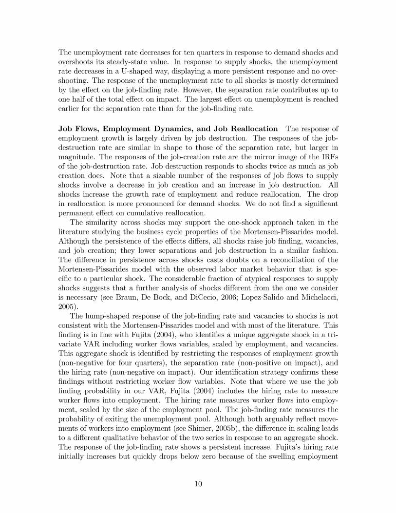
The unemployment rate decreases for ten quarters in response to demand shocks andovershoots its steady-state value. In response to supply shocks, the unemploymentrate decreases in a U-shaped way, displaying a more persistent response and no over-shooting. The response of the unemployment rate to all shocks is mostly determinedby the e¤ect on the job-�nding rate. However, the separation rate contributes up toone half of the total e¤ect on impact. The largest e¤ect on unemployment is reachedearlier for the separation rate than for the job-�nding rate.

Job Flows, Employment Dynamics, and Job Reallocation The response ofemployment growth is largely driven by job destruction. The responses of the job-destruction rate are similar in shape to those of the separation rate, but larger inmagnitude. The responses of the job-creation rate are the mirror image of the IRFsof the job-destruction rate. Job destruction responds to shocks twice as much as jobcreation does. Note that a sizable number of the responses of job �ows to supplyshocks involve a decrease in job creation and an increase in job destruction. Allshocks increase the growth rate of employment and reduce reallocation. The dropin reallocation is more pronounced for demand shocks. We do not �nd a signi�cantpermanent e¤ect on cumulative reallocation.The similarity across shocks may support the one-shock approach taken in the

literature studying the business cycle properties of the Mortensen-Pissarides model.Although the persistence of the e¤ects di¤ers, all shocks raise job �nding, vacancies,and job creation; they lower separations and job destruction in a similar fashion.The di¤erence in persistence across shocks casts doubts on a reconciliation of theMortensen-Pissarides model with the observed labor market behavior that is spe-ci�c to a particular shock. The considerable fraction of atypical responses to supplyshocks suggests that a further analysis of shocks di¤erent from the one we consideris necessary (see Braun, De Bock, and DiCecio, 2006; Lopez-Salido and Michelacci,2005).The hump-shaped response of the job-�nding rate and vacancies to shocks is not

consistent with the Mortensen-Pissarides model and with most of the literature. This�nding is in line with Fujita (2004), who identi�es a unique aggregate shock in a tri-variate VAR including worker �ows variables, scaled by employment, and vacancies.This aggregate shock is identi�ed by restricting the responses of employment growth(non-negative for four quarters), the separation rate (non-positive on impact), andthe hiring rate (non-negative on impact). Our identi�cation strategy con�rms these�ndings without restricting worker �ow variables. Note that where we use the job�nding probability in our VAR, Fujita (2004) includes the hiring rate to measureworker �ows into employment. The hiring rate measures worker �ows into employ-ment, scaled by the size of the employment pool. The job-�nding rate measures theprobability of exiting the unemployment pool. Although both arguably re�ect move-ments of workers into employment (see Shimer, 2005b), the di¤erence in scaling leadsto a di¤erent qualitative behavior of the two series in response to an aggregate shock.The response of the job-�nding rate shows a persistent increase. Fujita�s hiring rateinitially increases but quickly drops below zero because of the swelling employment

10

pool.The mildly negative e¤ect on cumulative reallocation is at odds with Caballero

and Hammour (2005), who �nd that expansionary aggregate shocks have positivee¤ects on cumulative reallocation.For monetary policy shocks, the IRFs of aggregate variables are consistent with

Christiano, Eichenbaum, and Evans (1999), who use a recursiveness restriction toidentify a monetary policy shock. However, Christiano, Eichenbaum, and Evans(1999) obtain a more persistent interest rate response and in�ation exhibits a pricepuzzle. The latter di¤erence is forced by our identi�cation scheme. The job �owsresponses are consistent with estimates in Trigari (2004) and the worker �ows andvacancies responses with those in Braun (2005).The last row of Figure 2 shows the IRFs of labor productivity for 100 quar-

ters. Average labor productivity, which is unrestricted, displays a persistent yet weakincrease in response to supply shocks. On the other hand, productivity shows no per-sistent response to demand and monetary shocks. The medium-run response of laborproductivity to supply shocks is consistent with a �technology shocks�interpretation.Table 5 reports the median of the posterior distribution of variance decompo-

sitions, i.e., the percentage of the j-periods-ahead forecast error accounted for bythe identi�ed shocks. The forecast errors of output and labor productivity are mostlydriven by supply shocks. Interestingly, demand shocks seem to play a more importantrole for the labor market variables than the supply shock. The greater importance ofdemand shocks suggests that more attention should be paid to other shocks in theevaluation of the basic labor market search model.A growing literature is analyzing the response of hours worked to technology

shocks in VARs. Shea (1999), Galì (1999, 2004), Basu, Fernald, and Kimball (2004),and Francis and Ramey (2005) argue that hours decrease on impact in response totechnology shocks. This result is at odds with the standard RBC model, whichimplies an increase in hours worked in response to a positive technology shock. Theconclusion drawn is that the RBC model should be amended by including nominalrigidities, habit formation in consumption and investment adjustment costs, a short-run �xed proportion technology, or di¤erent shocks.13 Our results on the importanceof demand shocks in driving labor-market variables and on atypical responses of thesevariables to supply shocks can be interpreted as an extension of the �negative hoursresponse��ndings, though in a milder form.Table 6 shows the variance contributions of the shocks at business cycle frequen-

cies. The contribution of shock i to the total variance is computed as follows:

� we simulate data with only shock i, say Zit ;

� we band-pass �lter Zit and Zt to obtain their business cycle components, (Zit)BC

and (Zt)BC , respectively;

� the contribution of shock i is computed by dividing the variance of (Zit)BC by

the variance of (Zt)BC .

13Christiano, Eichenbaum, and Vigfusson (2004), on the other hand, argue that the negativeimpact response of hours to technology shocks is an artifact of over-di¤erencing hours in VARs.

11

4.1 Matching Function Estimates

We can further analyze the possibly di¤erential response of the labor market to shocksby estimating a shock-speci�c matching function. In the Mortensen-Pissarides model,the number of hires is related to the size of the unemployment pool and the number ofvacancies via a matching functionM (U; V ).14 Assuming a Cobb-Douglass functionalform, the matching function is given by

M (U; V ) = AU�uV �v ;

where �v is the elasticity of the number of matches with respect to vacancies andmeasures the positive externality caused by �rms on searching workers; �u is theelasticity with respect to unemployment and measures the positive externality fromworkers to �rms; and A captures the overall e¢ ciency of the matching process.Under the assumption of constant returns to scale (CRS), i.e., �u + �v = 1, the

job-�nding rate can then be expressed as

ln ft = lnA+ � (ln vt � lnut) : (7)

If we do not impose CRS, we get

ln ft = lnA+ �v ln vt � (1� �u) ln ut:To consider the e¤ect of the shocks we identi�ed on the matching process, we con-

sider a sample of 1,000 draws from the posterior distributions of A and the elasticityparameters estimated from arti�cial data.Each draw involves the following steps:

1. consider a vector of accepted residuals constructed as if the shock(s) of interestwere the only structural shock(s);

2. use this vector of accepted residuals and the VAR parameters to generate arti-�cial data ~Zt;

3. construct unemployment using the steady-state approximation ~ut+1 = ~st=�~st + ~ft

�from the arti�cial data;

4. regress ln ~ft on either ln ~vt and ln ~ut (not assuming CRS) or ln (~vt=~ut) (underthe CRS assumption).

The arti�cial data constructed using only monetary shocks, for example, inducea posterior distribution for � and A for a hypothetical economy in which monetaryshocks are the only source of �uctuations.Table 7 reports the median, 16th, and 84th percentiles of 1,000 draws from the

posterior distributions for the output and price identi�cation scheme. The �rst two

14Petrongolo and Pissarides (2001) survey the matching function literature.

12

columns show the estimates for �v and A when we impose CRS. The CRS esti-mates suggest that aggregate shocks do not entail a di¤erential e¤ect on the match-ing process. The estimated e¢ ciency parameters A are somewhat lower for monetaryand demand shocks than for the supply shock, but the median estimates di¤er byless than 5%. The last three columns of Table 7 show the unrestricted estimates for�v, �u, and A. Estimates of �v and �u across shocks are close and the sum of thecoe¢ cients is around 0.70, corresponding to decreasing returns to scale. There are nosigni�cant di¤erences in the median estimates of the e¢ ciency parameter A.

5 Robustness

We analyze the robustness of our results by considering medium-run and long-runrestrictions on productivity to identify technology shocks. We also consider subsamplestability and a minimal VAR speci�cation to identify the shocks of interest.

5.1 Restricting the Medium-Run Response of Labor Produc-tivity

We push further the technological interpretation of supply shocks by identifying themas ones that increase labor productivity in the medium run. We leave unrestrictedthe short-run responses of output and the price level. This allows us to capture,as supply shocks, �news e¤ects�on future technological improvements (see Beaudryand Portier, 2003) and is akin to the long-run restrictions used in the literature. Wewill analyze the latter in the next subsection. The advantage of this medium-runrestriction is that it allows us to identify the other shocks within the same frameworkas above.In particular, we require that a technology shock raise labor productivity through-

out quarters 33 to 80 following the shock. The demand-side shocks, on the otherhand, are restricted to have no positive medium-run impact on labor productivity,while a¤ecting output, the price level, and the interest rate as above. The identify-ing restrictions are summarized in Table 4. This restriction is similar, in spirit, tothe long-run restriction on productivity adopted by Galì (1999). Uhlig (2004) andFrancis, Owyang, and Roush (2006) identify technology shocks in ways similar toours. According to Uhlig (2004), a technology shock is the only determinant of thek-periods-ahead forecast error variance. Francis, Owyang, and Roush (2006) identi-�cation is data-driven and attributes to technology shocks the largest share of thek-periods-ahead forecast error variance.Figures 4 and 5 report the median, 16th, and 84th percentiles of 1,000 draws from

the posterior distribution of acceptable IRFs to the structural shocks. By construc-tion, the demand-side shocks identi�ed satisfy the restrictions in the previous sectionas well. The responses of all variables to demand-side shocks and of output and in�a-tion to supply shocks are almost identical to the ones above. A sizable fraction (49.3percent) of the supply shocks identi�ed by restricting productivity in the mediumrun generate short-run responses of output and prices of opposite sign. Note that the

13

responses of the labor market variables to the supply shocks are smaller in absolutevalue than under the previous identi�cation scheme. Furthermore, a sizeable fractionof the responses of labor market variables points to a reduction in employment andhours and an increase in unemployment.For the variance decomposition displayed in Table 9, we again �nd that the two

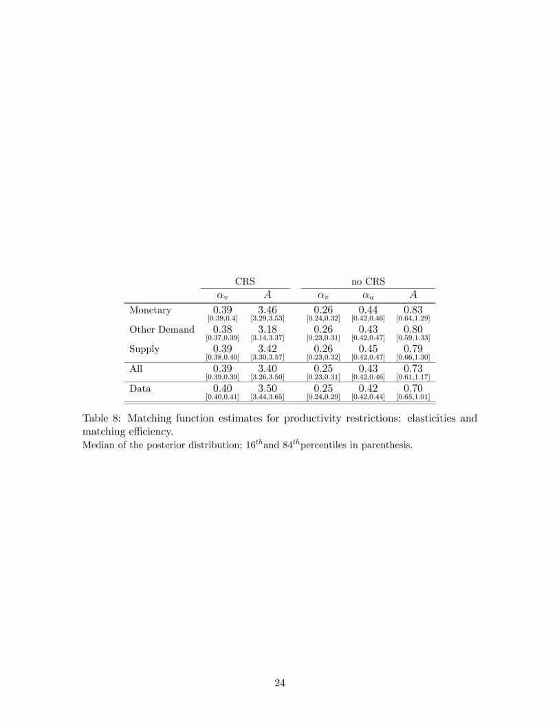
demand shocks are more important than supply shocks in driving �uctuations in labormarket variables. This is also true for the variance contributions at business cyclefrequencies, displayed in Table 6.Table 8 shows the matching function estimates under the labor productivity iden-

ti�cation scheme. The estimates are very similar. Now, only the e¢ ciency of thematching process in response to non-monetary demand shocks is lower than the cor-responding estimate for the supply shock under constant returns to scale.

5.2 Restricting Labor Productivity using a Long-Run Re-striction

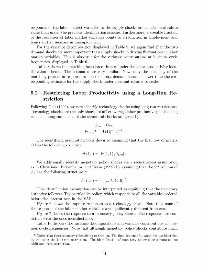
Following Galì (1999), we now identify technology shocks using long-run restrictions.Technology shocks are the only shocks to a¤ect average labor productivity in the longrun. The long-run e¤ects of the structural shocks are given by

Z1 = ��t;

� � [I � A (1)]�1A�10 :

The identifying assumption boils down to assuming that the �rst row of matrix� has the following structure:

�(1; :) = [� (1; 1) ; 01�9] :

We additionally identify monetary policy shocks via a recursiveness assumptionas in Christiano, Eichenbaum, and Evans (1999) by assuming that the 9th column ofA0 has the following structure15:

A0 (:; 9) = [01�9; A0 (9; 9)]0 :

This identi�cation assumption can be interpreted as signifying that the monetaryauthority follows a Taylor-rule-like policy, which responds to all the variables orderedbefore the interest rate in the VAR.Figure 6 shows the impulse responses to a technology shock. Note that none of

the response of the labor market variables are signi�cantly di¤erent from zero.Figure 7 shows the response to a monetary policy shock. The responses are con-

sistent with the ones identi�ed above.Table 10 displays the variance decompositions and variance contributions at busi-

ness cycle frequencies. Note that although monetary policy shocks contribute much

15Notice that there is one overidentifying restriction. The �rst element of �t would be just identi�edby imposing the long-run restriction. The identi�cation of monetary policy shocks imposes oneadditional zero restriction.

14

less to variance of output and productivity than the technology shocks, �uctuationsin the labor market variables are to a much larger extent driven by the monetaryshock.

5.3 Subsample Stability16

Several papers17 documented a drop in the volatility of output, in�ation, interestrates, and other macroeconomic variables since the early- or mid-1980s. Motivatedby these �ndings, we estimate our SVAR with pre-1984 and post-1984 subsamples.The post-1984 responses have similar shapes, but are smaller than the pre-1984 andthe whole sample responses for all the shocks. This is consistent with a reduction inthe volatility of the structural shocks. However, supply shocks have more persistente¤ects in the post-1984 subsample for both identi�cation schemes. The responsesof labor market variables to supply shocks identi�ed by restricting productivity areinsigni�cantly di¤erent from zero for both subsamples.In terms of forecast error decomposition, supply shocks are the most important

for output in the post-1984 subsamples; for hours, monetary shocks are the mostimportant in the pre-1984 subsample, while in the post-1984 subsamples the threeshocks we identify are equally important.18 For worker and job �ows, each demandshock is at least as important as the supply shock, across subsamples and identi�cationschemes.

5.4 Small VAR

To further check the robustness of our results, we used a lower-dimensional VAR con-taining labor productivity, in�ation, the nominal interest rate, and hours to identifythe shocks using the same sign restrictions as above. For a draw that satis�es theidentifying restrictions we then regressed

zt = a+TXj=0

�Mj b"Mt�j + TXj=0

�Dj b"Dt�j + TXj=0

�Sj b"St�j + �z;t;where

�"M ; "D; "S

�denote the three shocks identi�ed in the minimal VAR, zt is one

of the variables not contained in the VAR, i.e. either vacancies, the job-�nding rate,the separation rate, the job-creation rate, or the job-destruction rate. Also, a and �z;tdenote a constant and an i.i.d. error term, respectively. The length of the movingaverage terms was set to thirty, i.e., T = 30: The impulse responses for the labormarket variables are given by the respective �j.

16The full set of IRFs and variance decompositions for the two subsamples is available upon requestfrom the corresponding author.17See Kim and Nelson (1999), McConnell and Perez-Quiros (2000), and Stock and Watson (2003).18Our results on the increased importance in the later subsampes of supply shocks in accounting

for the forecast error of output are consistent with Fisher (2006). On the other hand, for hours,Fisher (2006) argues that the importance of technology shocks decreased post-1982.

15

For both identi�cation schemes, the qualitative conclusions are similar to above.The responses of the job-�nding rate and vacancies to a non-monetary demand shockare, however, less persistent then above. Furthermore, the responses to supply shocksare even less pronounced then for the VAR speci�cation discussed in Section 3 above.19

Again, demand shocks are as important as supply shocks in driving �uctuations ofthe labor market variables.

6 Conclusion

This paper considers alternative short-run, medium-run, and long-run restrictions toidentify structural shocks in order to analyze their impact on worker �ows, job �ows,vacancies, and hours. We �nd that demand shocks are more important than sup-ply shocks (technology shocks more speci�cally) in driving labor market �uctuations.When identi�ed via short-run price and output restrictions, supply shocks have qual-itatively similar e¤ects to demand shocks. They raise employment, vacancies, thejob-creation rate, and the job-�nding rate while lowering unemployment, separationsand job destruction. These e¤ects are more persistent for supply shocks. When iden-ti�ed via medium-run or long-run restrictions on labor productivity, however, supplyshocks do not have a clear cut e¤ect on the labor market variables.

19The �gures are available upon request.

16

References

Basu, S., J. Fernald, and M. Kimball (2004): �Are Technology ImprovementsContractionary?,� NBER Working Papers 10592, National Bureau of EconomicResearch, Inc.

Beaudry, P., and F. Portier (2003): �Stock Prices, News and Economic Fluctu-ations,�unpublished manuscript, University of British Columbia.

Blanchard, O. J., and P. Diamond (1990): �The Cyclical Behavior of the GrossFlows of U. S. Workers,�Brookings Papers on Economic Activity, 0(2), 85�143.

Braun, H. (2005): �(Un)Employment Dynamics: The Case of Monetary PolicyShocks,�unpublished manuscript, University of British Columbia.

Braun, H., R. De Bock, and R. DiCecio (2006): �Aggregate Shocks and LaborMarket Fluctuations,�Federal Reserve Bank of St. Louis WP 2006-004A.

Caballero, R. J., and M. L. Hammour (2005): �The Cost of Recessions Revis-ited: A Reverse-Liquidationist View,�Review of Economic Studies, 72(2), 313�341.

Christiano, L., M. Eichenbaum, and C. Evans (1999): �Monetary PolicyShocks: What Have We Learned and to What End?,� in Handbook of Macro-economics, ed. by J. B. Taylor, and M. Woodford, vol. 1A, chap. 1, pp. 65�148.Elsevier Science, North-Holland, Amsterdam, New York and Oxford.

Christiano, L. J., M. Eichenbaum, and R. Vigfusson (2004): �The Responseof Hours to a Technology Shock: Evidence Based on Direct Measures of Technol-ogy,�Journal of the European Economic Association, 2(2-3), 381�95.

Christiano, L. J., and T. J. Fitzgerald (2003): �The Band Pass Filter,�Inter-national Economic Review, 44(2), 435�465.

Davis, S. J., R. J. Faberman, and J. Haltiwanger (2005): �The Flow Ap-proach to Labor Markets: New Data Sources, Micro-Macro Links and the RecentDownturn,�Discussion Paper 1639, Institute for the Study of Labor (IZA).

Davis, S. J., and J. Haltiwanger (1999): �On the Driving Forces behind CyclicalMovements in Employment and Job Reallocation,�American Economic Review,89(5), 1234�58.

Davis, S. J., and J. C. Haltiwanger (1992): �Gross Job Creation, Gross Job De-struction, and Employment Reallocation,�Quarterly Journal of Economics, 107(3),819�63.

Davis, S. J., J. C. Haltiwanger, and S. Schuh (1996): Job creation and de-struction. The MIT Press, Boston, MA.

17

Faberman, R. J. (2004): �Gross Job Flows over the Past Two Business Cycles: Notall �Recoveries�are Created Equal,�Discussion Paper 372, U.S. Bureau of LaborStatistics.

Fisher, J. D. M. (2006): �The Dynamic E¤ects of Neutral and Investment-Speci�cTechnology Shocks,�Journal of Political Economy, 114(3), 413�51.

Francis, N., M. T. Owyang, and J. E. Roush (2006): �A �exible �nite-horizonidenti�cation of technology shocks,� Working Papers 2005-024, Federal ReserveBank of St. Louis.

Francis, N., and V. A. Ramey (2005): �Is the Technology-Driven Real BusinessCycle Hypothesis Dead? Shocks and Aggregate Fluctuations Revisited,�Journalof Monetary Economics, 52(8), 1379�99.

Fujita, S. (2004): �Vacancy persistence,� Federal Reserve Bank of Philadelphia,Working Paper No. 04-23.

Galì, J. (1999): �Technology, Employment, and the Business Cycle: Do TechnologyShocks Explain Aggregate Fluctuations?,�American Economic Review, 89(1), 249�71.

(2004): �On the Role of Technology Shocks as a Source of Business Cycles:Some New Evidence,�Journal of the European Economic Association, 2(2-3), 372�80.

Hagedorn, M., and I. Manovskii (2006): �The Cyclical Behavior of EquilibriumUnemployment and Vacancies Revisited,�Working Paper, University of Pennsyl-vania.

Hall, R. E. (2005): �Job Loss, Job Finding, and Unemployment in the U.S. Econ-omy over the Past Fifty Years,�in NBER Macroeconomics Annual 2005, Vol. 20,ed. by M. Gertler, and K. Rogo¤. The MIT Press, Boston, MA, forthcoming.

Jeffreys, H. (1961): Theory of Probability. Oxford University Press, London, 3rdedn.

Kim, C.-J., and C. R. Nelson (1999): �Has The U.S. Economy Become More Sta-ble? A Bayesian Approach Based On A Markov-Switching Model Of The BusinessCycle,�The Review of Economics and Statistics, 81(4), 608�616.

Lopez-Salido, J. D., and C. Michelacci (2005): �Technology Shocks and JobFlows,�unpublished manuscript, CEMFI.

McConnell, M. M., and G. Perez-Quiros (2000): �Output Fluctuations in theUnited States: What Has Changed since the Early 1980�s?,�American EconomicReview, 90(5), 1464�1476.

18

Mortensen, D., and E. Nagypal (2005): �More on Unemployment and VacancyFluctuations,� NBER Working Papers 11692, National Bureau of Economic Re-search, Inc.

Mortensen, D. T., and C. A. Pissarides (1994): �Job Creation and Job De-struction in the Theory of Unemployment,�Review of Economic Studies, 61(3),397�415.

Peersman, G. (2005): �What Caused the Early Millenium Slowdown? EvidenceBased on Vector Autoregressions.,�Journal of Applied Econometrics, 20(2), 185�207.

Petrongolo, B., and C. A. Pissarides (2001): �Looking into the Black Box: ASurvey of the Matching Function,�Journal of Economic Literature, 39(2), 390�431.

Shea, J. (1999): �What Do Technology Shocks Do?,� in NBER macroeconomicsannual 1998, ed. by B. S. Bernanke, and J. J. e. Rotemberg. The MIT Press.

Shimer, R. (2004): �The Consequences of Rigid Wages in Search Models,�Journalof the European Economic Association, 2(2-3), 469�79.

(2005a): �The Cyclicality of Hires, Separations, and Job-to-Job Transitions,�Federal Reserve Bank of St. Louis Review, 87(4), 493�508.

(2005b): �Reassessing the Ins and Outs of Unemployment,� unpublishedmanuscript, University of Chicago.

Silva, J. I., and M. Toledo (2005): �Labor Turnover Costs and the CyclicalBehavior of Vacancies and Unemployment,�2005 Meeting Papers 775, Society forEconomic Dynamics.

Stock, J. H., and M. W. Watson (2003): �Has the Business Cycle Changed andWhy?,�in NBER Macroeconomics Annual 2002, ed. by M. Gertler, and K. Rogo¤.The MIT Press, Boston, MA, forthcoming.

Trigari, A. (2004): �Equilibrium unemployment, job �ows and in�ation dynamics,�European Central Bank, Working Paper No. 304.

Uhlig, H. (2004): �Do Technology Shocks Lead to a Fall in Total Hours Worked?,�Journal of the European Economic Association, 2(2-3), 361�71.

(2005): �What are the e¤ects of monetary policy on output? Results froman agnostic identi�cation procedure,�Journal of Monetary Economics, 52(2), 381�419.

19

fs

JC

JD

uv

hAPL

y

f6:27

[5:54;6:99]

�0:48

[�0:63;�0:29]

�0:04

[�0:24;0:15]

�0:53

[�0:66;�0:39]

�0:98

[�0:99;�0:96]

0:95

[0:93;0:97]

0:96

[0:93;0:98]

0:20

[�0:03;0:4]

0:88

[0:81;0:92]

s2:55

[2:21;2:99]

�0:55

[�0:68;�0:37]

0:86

[0:78;0:91]

0:54

[0:39;0:66]

�0:62

[�0:73;�0:49]

�0:48

[�0:61;�0:33]

�0:63

[�0:77;�0:44]

�0:67

[�0:78;�0:53]

JC

4:26

[3:61;4:97]

�0:58

[�0:7;�0:41]

0:08

[�0:10;0:26]

0:04

[�0:17;0:24]

�0:11

[�0:3;0:09]

0:53

[0:33;0:68]

0:14

[�0:11;0:36]

JD

6:73

[5:89;7:59]

0:53

[0:40;0:63]

�0:65

[�0:76;�0:53]

�0:53

[�0:66;�0:39]

�0:70

[�0:82;�0:54]

�0:72

[�0:84;�0:58]

u7:27

[6:39;8:24]

�0:95

[�0:96;�0:93]

�0:95

[�0:97;�0:92]

�0:18

[�0:38;0:01]

�0:86

[�0:90;�0:81]

v8:84

[8:13;9:78]

0:95

[0:94;0:97]

0:34

[0:14;0:53]

0:94

[0:9;0:96]

h1:10

[1:01;1:19]

0:17

[�0:06;0:38]

0:89

[0:84;0:93]

APL

0:65

[0:56;0:77]

0:58

[0:43;0:7]

y1

[NA]

Table1:Correlationmatrixofbusiness-cyclecomponents.

Standarddeviations(relativetooutput)areshownon

thediagonal.AllserieswereloggedanddetrendedusingaBP(8,32)�lter.

Block-bootstrappedcon�denceintervalsinbrackets.

20

Levels BC componentst

st+ft�s

�s+ftstst+ �f

stst+ft

�s�s+ft

stst+ �f

Corr(x; ut+1) 0:99[0:99;1]

0:85[0:76;0:92]

0:79[0:64;0:87]

0:99[0:99;1]

0:93[0:90;0:95]

0:74[0:62;0:82]

Std(x) =Std(ut+1) 1:01[1;1:03]

0:69[0:6;0:82]

0:49[0:42;0:58]

1:03[1:01;1:05]

0:79[0:73;0:86]

0:31[0:28;0:36]

Table 2: Contribution of the job �nding and separation rates to unemployment: levelsand business-cycle components.The business cycle component is extracted with a BP(8,32) �lter. Block-bootstrappedcon�dence intervals in brackets.

Demand shocks Supply shocksVariable Monetary OtherOutput " 1� 4 " 1� 4 " 1� 4Price level " 1� 4 " 1� 4 # 1� 4Interest rate # 1 " 1 �

Table 3: Sign restrictions: demand and supply shocks

Demand shocks Supply shocksVariable Monetary Other

not " 33� 80 not " 33� 80 " 33� 80Output " 1� 4 " 1� 4 �Price level " 1� 4 " 1� 4 �Interest rate # 1 " 1 �

Table 4: Sign restrictions: demand and supply shocks

21

48

2032

MD

SM

DS

MD

SM

DS

Output

9:5

[2:7;23:8]

6:4

[1:6;19:9]

13:4

[3:8;30:9]

8:1

[2:5;21:3]

5:8

[2:4;13:4]

14:4

[4:4;32:5]

7:1

[2:8;15:5]

7:0

[2:5;16:7]

12:3

[3:9;28:2]

6:7

[2:8;15:1]

6:9

[2:7;6:9]

11:5

[3:7;26:3]

In�ation

6:8

[2:1;18:6]

8:6

[2:4;24:8]

9:5

[2:3;27:8]

8:4

[2:5;21:3]

9:6

[2:8;26:4]

8:5

[2:4;23:7]

8:7

[2:9;21:5]

9:6

[3:7;23:4]

9:0

[3:3;21:3]

9:1

[3:4;19:7]

10:2

[4:2;10:2]

9:3

[3:7;20:9]

Int.rate

4:8

[1:6;11:7]

19:6

[5:4;29:6]

5:2

[1:3;18:3]

6:9

[2:4;14:8]

20:0

[6:4;38:4]

5:4

[1:6;14:9]

7:7

[3:0;17:1]

17:7

[6:9;32:3]

7:0

[2:5;15:0]

8:0

[3:3;16:4]

16:3

[6:9;16:3]

8:0

[3:3;15:7]

Hours

8:4

[1:2;26:6]

7:8

[1:4;26:5]

8:5

[1:4;27:4]

8:9

[1:8;25:5]

6:0

[1:9;17:1]

10:9

[2:2;29:8]

8:6

[2:8;19:2]

9:0

[3:0;19:2]

10:8

[3:2;25:1]

9:1

[3:1;18:9]

9:2

[3:5;9:2]

10:4

[3:8;22:8]

JobFinding

9:3

[2:0;27:8]

6:8

[1:7;22:8]

8:2

[2:2;25:7]

9:4

[1:9;26:3]

6:1

[2:2;16:0]

10:4

[2:5;28:7]

8:5

[2:7;18:7]

10:7

[4:1;21:6]

10:0

[3:2;25:4]

8:6

[3:1;18:6]

11:2

[4:4;11:2]

10:1

[3:5;23:8]

Separation

8:7

[2:7;22:5]

6:3

[1:7;18:0]

8:8

[2:4;22:3]

8:5

[3:2;19:8]

8:5

[3:3;17:7]

10:0

[3:3;21:9]

8:8

[3:8;16:7]

10:0

[4:2;18:5]

10:8

[4:0;21:1]

8:6

[3:8;15:3]

9:5

[4:3;9:5]

11:0

[4:4;20:7]

JC7:2

[2:1;20:9]

9:7

[3:5;21:7]

7:2

[2:5;19:0]

8:6

[3:4;18:7]

12:6

[5:4;22:8]

7:8

[3:1;18:0]

9:6

[4:3;20:0]

12:5

[5:7;22:1]

8:4

[3:6;17:4]

9:6

[4:4;19:5]

12:5

[5:7;12:5]

8:4

[3:7;17:3]

JD11:5

[3:8;27:8]

10:3

[2:7;26:1]

6:6

[2:2;17:9]

11:4

[4:1;24:9]

11:9

[4:1;24:8]

7:5

[3:0;;17:5]

11:3

[4:4;25:3]

12:7

[4:9;25:3]

7:5

[3:1;16:5]

11:2

[4:4;24:9]

12:8

[5:1;12:8]

7:7

[3:2;16:1]

Vacancies

9:0

[1:0;27:0]

5:5

[1:1;19:4]

7:9

[1:1;25:9]

8:5

[1:4;25:5]

6:3

[2:5;14:6]

9:3

[1:6;27:8]

9:0

[3:0;18:3]

11:5

[4:3;24:3]

8:6

[2:5;22:0]

9:3

[3:3;18:7]

11:4

[4:7;11:4]

8:8

[3:3;20:8]

APL

4:4

[1:0;16:5]

4:8

[1:4;15:7]

7:7

[1:4;27:9]

4:6

[1:4;14:9]

5:7

[1:6;16:6]

7:4

[1:6;24:7]

4:5

[1:3;14:3]

5:4

[1:5;17:0]

6:6

[1:6;22:7]

4:5

[1:3;14:5]

5:5

[1:5;5:5]

7:4

[1:7;24:2]

Table5:Variancedecompositionsforoutputandpricerestrictions:percentageofthej-periodsaheadforecasterrorexplained

bymonetary(M),otherdemand(D),andsupplyshocks(S).Numbersinbracketsare16thand84thpercentilesobtainedfrom

abootstrapwith1.000draws.

22

Price-Output Restriction Labor Productivity RestrictionMonetary Demand Supply Monetary Demand Supply

Output 9:3[3:4;20:6]

12:5[4:3;25:9]

9:8[2:9;23:5]

8:8[3:4;19:6]

12:3[4:7;25:1]

7:5[2:0;19:4]

In�ation 6:1[1:7;16:1]

12:4[4:3;29:5]

10:3[3:4;25:2]

6:6[2:0;15:0]

13:9[4:7;28:8]

8:8[2:4;22:4]

Int. rate 6:5[2:3;14:3]

15:5[4:7;33:6]

5:8[1:6;14:4]

6:4[2:4;13:7]

16:0[6:0;33:9]

6:2[1:8;16:8]

Hours 9:3[2:6;24:1]

13:8[4:0;31:6]

9:1[2:6;23:1]

8:8[2:5;22:2]

14:8[4:8;32:2]

7:8[2:1;20:5]

Job Finding 9:5[2:6;24:3]

12:8[3:5;31:1]

9:2[2:8;22:5]

9:5[3:3;22:8]

13:8[4:2;30:6]

8:0[2:1;20:5]

Separation 9:3[3:6;22:0]

10:9[3:4;27:6]

8:7[2:7;29:8]

9:9[3:7;20:8]

11:2[3:7;27:3]

8:1[2:6;19:4]

JC 7:3[2:3;18:7]

11:4[4:4;24:1]

6:2[1:8;15:7]

7:1[2:4;19:2]

11:6[4:6;23:5]

6:6[2:1;16:6]

JD 9:5[2:9;22:8]

13:3[3:6;28:7]

6:3[1:8;16:3]

9:3[3:4;20:8]

13:7[4:1;29:7]

7:1[1:8;16:6]

Vacancies 9:7[2:3;23:0]

12:5[3:9;27:4]

8:6[2:3;22:0]

9:1[2:7;22:7]

13:0[4:6;28:3]

8:0[2:0;19:7]

APL 7:5[2:817:0]

10:5[3:6;20:8]

8:8[2:6;21:1]

7:4[2:7;16:4]

9:9[4:0;20:8]

8:5[2:7;20:9]

Table 6: Variance Contributions at the Business Cycle Frequency in percent, see text.Numbers in brackets are 16th and 84th percentiles obtained from a bootstrap with1.000 draws.

CRS no CRS�v A �v �u A

Monetary 0:39[0:38;0:40]

3:35[3:30;3:58]

0:27[0:24;0:30]

0:44[0:42;0:47]

0:81[0:65;1:14]

Other Demand 0:39[0:38;0:40]

3:33[3:24;3:52]

0:27[0:25;0:31]

0:46[0:44;0:48]

0:92[0:77;1:29]

Supply 0:41[0:41;0:42]

3:69[3:61;3:86]

0:27[0:25;0:31]

0:43[0:43;0:44]

0:85[0:72;1:14]

All 0:40[0:40;0:41]

3:54[3:49;3:69]

0:25[0:25;0:29]

0:43[0:43;0:44]

0:75[0:69;1:01]

Data 0:40[0:40;0:41]

3:55[3:44;3:66]

0:25[0:25;0:29]

0:43[0:43;0:43]

0:74[0:70;1:02]

Table 7: Matching function estimates for output and price restrictions: elasticitiesand matching e¢ ciency.Median of the posterior distribution; 16thand 84thpercentiles in parenthesis.

23

CRS no CRS�v A �v �u A

Monetary 0:39[0:39;0:4]

3:46[3:29;3:53]

0:26[0:24;0:32]

0:44[0:42;0:46]

0:83[0:64;1:29]

Other Demand 0:38[0:37;0:39]

3:18[3:14;3:37]

0:26[0:23;0:31]

0:43[0:42;0:47]

0:80[0:59;1:33]

Supply 0:39[0:38;0:40]

3:42[3:30;3:57]

0:26[0:23;0:32]

0:45[0:42;0:47]

0:79[0:66;1:30]

All 0:39[0:39;0:39]

3:40[3:26;3:50]

0:25[0:23;0:31]

0:43[0:42;0:46]

0:73[0:61;1:17]

Data 0:40[0:40;0:41]

3:50[3:44;3:65]

0:25[0:24;0:29]

0:42[0:42;0:44]

0:70[0:65;1:01]

Table 8: Matching function estimates for productivity restrictions: elasticities andmatching e¢ ciency.Median of the posterior distribution; 16thand 84thpercentiles in parenthesis.

24

48

2032

MD

SM

DS

MD

SM

DS

Output

8:0

[2:2;21:5]

5:4

[1:3;16:0]

7:6

[1:4;24:3]

7:2

[2:0;18:5]

5:3

[2:3;10:8]

8:3

[2:0;26:4]

5:8

[2:2;13:0]

6:5

[2:614:5;]

10:4

[3:1;26:0]

5:1

[2:0;11:5]

5:7

[2:3;12:9]

10:9

[3:8;26:2]

In�ation

7:0

[2:4;19:0]

8:7

[2:7;23:7]

6:9

[1:8;22:3]

9:1

[2:9;20:8]

10:6

[3:4;24:7]

7:6

[2:2;20:6]

10:2

[3:8;21:8]

10:7

[4:1;22:6]

8:3

[2:8;28:9]

10:7

[4:5;20:3]

11:5

[5:0;21:8]

8:2

[3:0;18:2]

Int.rate

4:5

[1:8;10:4]

19:5

[6:5;41:4]

5:6

[1:3;18:3]

6:5

[2:4;13:8]

20:5

[7:4;29:7]

6:4

[1:7;16:7]

7:3

[3:0;16:8]

20:5

[7:4;32:7]

8:0

[2:6;16:8]

7:9

[3:3;15:9]

16:8

[7:7;28:5]

8:3

[3:1;17:3]

Hours

7:1

[0:9;24:5]

8:0

[1:4;25:8]

6:4

[1:1;21:4]

7:3

[1:2;25:4]

6:1

[2:0;16:9]

6:8

[1:5;20:8]

9:0

[3:4;18:8]

6:1

[4:0;20:1]

7:3

[2:2;18:6]

10:4

[3:8;20:1]

11:2

[4:9;20:9]

7:3

[2:5;17:3]

JobFinding

9:5

[2:9;27:0]

7:3

[1:9;20:9]

6:1

[1:4;19:6]

9:8

[2:6;25:0]

6:4

[2:5;14:7]

6:6

[1:7;19:9]

8:5

[3:2;18:7]

6:4

[4:7;21:5]

7:8

[2:4;19:4]

9:1

[3:5;19:5]

11:8

[5:1;21:7]

7:9

[2:7;19:1]

Separation

8:9

[2:7;21:8]

6:2

[1:9;19:4]

7:4

[2:1;20:5]

8:5

[3:2;18:7]

8:7

[3:6;18:3]

8:4

[2:9;19:9]

8:8

[4:2;16:0]

8:8

[4:7;18:7]

9:3

[3:8;19:0]

8:9

[4:8;15:4]

10:1

[5:0;17:2]

9:3

[3:9;19:2]

JC7:4

[2:2;23:2]

9:3

[3:4;21:1]

7:4

[2:8;19:5]

8:8

[3:6;20:1]

12:4

[5:7;21:9]

8:2

[3:3;18:7]

9:8

[4:3;20:4]

12:4

[6:3;21:6]

8:4

[3:6;17:8]

9:9

[4:4;20:1]

12:5

[6:5;21:4]

8:5

[3:8;17:6]

JD11:2

[4:2;26:1]

10:5

[2:9;26:1]

6:9

[2:2;18:6]

10:9

[4:4;23:4]

11:9

[4:5;24:6]

7:7

[2:9;17:6]

11:1

[4:8;23:1]

11:9

[5:5;25:3]

7:8

[3:0;16:8]

11:1

[5:0;23:0]

13:2

[5:7;25:4]

7:9

[3:2;16:7]

Vacancies

8:8

[1:2;26:8]

5:2

[1:1;19:8]

6:5

[0:8;21:4]

7:6

[1:6;24:5]

6:5

[2:5;14:7]

7:0

[1:4;21:2]

8:6

[3:0;18:5]

6:5

[4:9;23:5]

7:8

[2:5;18:6]

9:0

[3:4;19:5]

12:3

[5:3;23:3]

8:4

[3:1;17:8]

APL

4:9

[0:9;17:8]

4:5

[1:4;12:8]

7:6

[1:5;26:0]

5:2

[1:4;15:1]

5:7

[1:7;15:4]

8:0

[1:7;25:4]

5:5

[1:4;15:5]

5:7

[1:7;16:2]

7:7

[1:5;25:4]

5:0

[1:4;14:0]

5:7

[1:5;15:4]

8:1

[1:7;26:0]

Table9:Variancedecompositionsforproductivityrestriction:percentageofthej-periodsaheadforecasterrorexplainedby

monetary(M),otherdemand(D),andsupplyshocks(S).Numbersinbracketsare16thand84thpercentilesobtainedfrom

abootstrapwith1.000draws.

25

48

2032

BusinessCycle

MTech

MTech

MTech

MTech

MTech

Output

5:9

[3:3;9:6]

21:4

[10:9;41:5]

14:2

[8:1;19:7]

35:1

[22:0;51:7]

10:4

[5:4;14:3;]

56:1

[39:4;66:9]

12:1

[4:1;11:6]

64:0

[47:4;73:8]

12:1

[7:7;23:6]

15:1

[6:0;25:2]

In�ation

1:2

[0:3;2:9]

25:7

[4:33;32:6]

0:9

[0:7;3:3]

26:4

[5:0;32:7]

1:4

[1:4;6:2]

25:8

[6:0;30:8]

3:3

[1:5;6:3]

24:9

[6:7;30:7]

3:3

[1:8;8:9]

30:3

[4:0;31:2]

Int.rate

50:5

[38:4;54:0]

5:7

[0:7;10:8]

32:9

[23:9;38:9]

6:1

[1:0;12:5]

26:3

[19:2;32:3]

5:4

[1:6;12:3]

32:3

[16:6;28:3]

6:6

[2:8;14:6]

32:3

[26:6;51:6]

6:1

[1:2;12:0]

Hours

4:4

[2:4;7:9]

1:3

[0:8;10:7]

17:1

[10:0;24:4]

6:9

[2:1;16:2]

18:4

[9:7;23:6]

21:4

[4:5;26:6]

14:6

[8:8;22:0]

22:3

[4:8;27:4]

14:6

[8:1;25:5]

7:9

[2:1;13:1]

Job�nding

5:2

[2:9;9:1]

2:;2

[1:1;9:7]

18:6

[11:4;27:0]

2:7

[1:9;11:1]

22:7

[12:7;28:5]

9:2

[3:0;17:9]

14:6

[12:1;27:3]

9:3

[3:3;18:4]

14:6

[8:1;26:1]

9:1

[2:1;13:6]

Separation

9:4

[5:6;13:9]

1:8

[1:2;7:5]

16:7

[9:7;21:4]

4:3

[2:4;9:9]

12:8

[7:5;17:2]

9:9

[3:5;15:5]

16:5

[6:1;14:6]

13:6

[4:3;20:3]

16:5

[9:7;24:8]

7:4

[2:0;12:1]

JC4:9

[2:5;8:1]

3:3

[2:1;9:2]

4:9

[2:8;8:2]

5:5

[2:5;11:3]

5:4

[4:0;10:1]

5:5

[2:8;11:4]

6:6

[4:0;10:1]

5:5

[3:0;11:5]

6:6

[4:9;14:7]

4:1

[1:5;10:4]

JD9:9

[6:1;14:9]

3:4

[1:3;9:1]

17:6

[10:8;22:4]

4:2

[1:8;9:7]

16:2

[10:27;21:4]

4:4

[2:0;10:2]

13:3

[10:3;21:4]

4:7

[2:1;10:4]

13:4

[9:0;23:5]

5:3

[1:4;11:6]

Vacancies

10:6

[6:5;15:5]

0:5

[0:2;7:4]

25:0

[15:6;31:7]

3:0

[1:4;10:4]

21:7

[12:5;26:6]

6:3

[2:3;15:1]

17:3

[10:9;24:0]

6:2

[3:5;15:9]

17:3

[10:1;29:6]

7:5

[2:0;12:8]

APL

2:1

[0:8;4:3]

37:1

[22:3;69:3]

1:6

[0:7;3:7]

41:2

[26:1;74:8]

0:8

[0:7;3:5]

42:4

[29:0;80:6]

6:2

[0:6;7:1]

47:0

[36:2;84:8]

6:2

[3:6;12:5]

25:7

[14:3;50:5]

Table10:Variancedecompositionsforrecursivenessandlong-runrestrictions:percentageofthej-periodsaheadforecasterror

explainedbymonetary(M)andtechnologyshocks(Tech).Thelastcolumnpresentsthevariancecontributionsatthebusiness

cyclefrequency(seetext).Numbersinbracketsare16thand84thpercentilesobtainedfrom

abootstrapwith10.000draws.

..

26

Q3­54 Q4­62 Q1­71 Q2­79 Q3­87 Q4­95 Q1­04

­0.8­0.6­0.4­0.2

log(ft)

Q3­54 Q4­62 Q1­71 Q2­79 Q3­87 Q4­95 Q1­04­0.2

0

0.2

log(ft): BC component

Q3­54 Q4­62 Q1­71 Q2­79 Q3­87 Q4­95 Q1­04

­3.5

­3

log(st)

Q3­54 Q4­62 Q1­71 Q2­79 Q3­87 Q4­95 Q1­04

­0.050

0.05

log(st): BC component

Q3­54 Q4­62 Q1­71 Q2­79 Q3­87 Q4­95 Q1­04

­3.2­3

­2.8­2.6

log(JCt)

Q3­54 Q4­62 Q1­71 Q2­79 Q3­87 Q4­95 Q1­04

­0.10

0.1

log(JCt): BC component

Q3­54 Q4­62 Q1­71 Q2­79 Q3­87 Q4­95 Q1­04

­3

­2.5

log(JD t)

Q3­54 Q4­62 Q1­71 Q2­79 Q3­87 Q4­95 Q1­04

­0.2

0

0.2

log(JD t): BC component

Figure 1: Worker and job �ows: levels and business-cycle components.The business-cycle component is extracted with a BP(8,32) �lter. Shaded areas denote theNBER recessions.

27

­0.5

0

0.5

ln(Y

)

Monetary

­0.5

0

0.5

Other demand

­0.5

0

0.5

Supply

­0.5

0

0.5

π

­0.5

0

0.5

­0.5

0

0.5

­0.20

0.20.4

ln(1

+R)

­0.20

0.20.4

­0.20

0.20.4

0 5 10 15 20­0.4­0.2

00.20.40.6

ln(H

)

0 5 10 15 20­0.4­0.2

00.20.40.6

0 5 10 15 20­0.4­0.2

00.20.40.6

0 20 40 60 80­0.4­0.2

00.20.40.6

ln(Y

/H)

0 20 40 60 80­0.4­0.2

00.20.40.6

0 20 40 60 80­0.4­0.2

00.20.40.6

Figure 2: Price Restriction: IRFs for non-labor market variables and hours (%):demand and supply shocks.Median (solid), 16th and 84th percentiles (dashed) of posterior distributions.

28

­0.50

0.5

ln(Y

)

M onetary

­0.50

0.5

O ther demand

­0.50

0.5

Supply

­202

ln(f)

­ 202

­202

­1.5­1­0.500.5

ln(s

)

­ 1.5­1­0.500.5

­1.5­1­0.500.5

­1012

ln(J

C)

­ 1012

­1012

­4­2

0

ln(J

D)

­ 4­2

0

­4­2

0

­4­2

024

ln(v

)

­ 4­2

024

­4­2

024

­0.10

0.1

u t+1

­0.10

0.1

­0.10

0.1

­20246

g E,t+

1

­20246

­20246

­202

Real

loca

tion

­ 202

­202

0 5 10 15 20­15­10­5

05

Cum

ulat

ive

Real

loca

tion

0 5 10 15 20­15­10­5

05

0 5 10 15 20­15­10­5

05

Figure 3: Price Restriction: IRFs for labor market variables (%): demand and supplyshocks.Median (solid), 16th and 84th percentiles (dashed) of posterior distributions.

29

­0.5

0

0.5

ln(Y

)

Monetary

­0.5

0

0.5

Other demand

­0.5

0

0.5

Supply

­0.5

0

0.5

π

­0.5

0

0.5

­0.5

0

0.5

­0.20

0.20.4

ln(1

+R)

­0.20

0.20.4

­0.20

0.20.4

0 5 10 15 20­0.5

0

0.5

ln(H

)

0 5 10 15 20­0.5

0

0.5

0 5 10 15 20­0.5

0

0.5

0 20 40 60 80­0.5

0

0.5

ln(Y

/H)

0 20 40 60 80­0.5

0

0.5

0 20 40 60 80­0.5

0

0.5

Figure 4: Labor Productivity Restriction: IRFs for non-labor market variables andhours (%): demand and supply shocks.Median (solid), 16th and 84th percentiles (dashed) of posterior distributions.

30

­0.50

0.5

ln(Y

)

M onetary

­0.50

0.5

O ther demand

­0.50

0.5

Supply

­202

ln(f)

­ 202

­202

­101

ln(s

)

­ 101

­101

­1012

ln(J

C)

­ 1012

­1012

­4­2

02

ln(J

D)

­ 4­2

02

­4­2

02

­4­2

024

ln(v

)

­ 4­2

024

­4­2

024

­0.10

0.1

u t+1

­0.10

0.1

­0.10

0.1

­20246

g E,t+

1

­20246

­20246

­202

Real

loca

tion

­ 202

­202

0 5 10 15 20

­100

10

Cum

ulat

ive

Real

loca

tion

0 5 10 15 20

­100

10

0 5 10 15 20

­100

10

Figure 5: Labor Productivity Restriction: IRFs for labor market variables (%): de-mand and supply shocks.Median (solid), 16th and 84th percentiles (dashed) of posterior distributions.

31

0

0.5

1

Output

­0.8­0.6­0.4­0.2

0Inflation

­0.4

­0.2

0

Interest rate

­0.20

0.20.40.60.8

Hours

­202

Job­finding rate

­1

0

1

Separation rate

­1012

Job creation

­10123

Job destruction

0 5 10 15 20­2

024

Vacancies

0 5 10 15 20

0.20.40.60.8

Labor productivity

Figure 6: IRF�s to a technology shock identi�ed with a long-run restriction on pro-ductivity.

32

00.20.40.60.8

Output

­0.2­0.1

00.1

Inflation

­0.8­0.6­0.4­0.2

00.2

Interest rate

00.20.40.6

Hours

0

2

4Job­finding rate

­1.5­1

­0.50

Separation rate

­0.50

0.51

1.5

Job creation

­3­2­1

01

Job destruction

0 5 10 15 20

0246

Vacancies

0 5 10 15 20­0.2

0

0.2

Labor productivity

Figure 7: IRF�s to a monetary shock identi�ed with a contemporaneous restriction.

33

Variable Units Haver (USECON)

Civilian Noninstitutional Population Thousands, NSA LN16NOutput per hour all persons (Nonfarm Business Sector) Index, 1992=100, SA LXNFAOutput (Nonfarm Business Sector) Index, 1992=100, SA LXNFOGDP: Chain Price Index Index, 2000=100, SA JGDPReal GDP Bil. Chn. 2000 $, SAAR GDPHFederal Funds (e¤ective) Rate % p.a. FFEDHours of all persons (Nonfarm Bus. Sector) Index, 1992=100, SA LXNFHIndex of Help-Wanted Advertising in Newspapers Index, 1987=100, SA LHELPCivilian Labor Force (16yrs +) Thousands, SA LFCivilian Unemployment Rate (16yrs +) %, SA LR

Table A.1: Other data

A Other Data

Table A.1 describes the data (other than the job �ows and worker �ows data) usedin the paper and provides the corresponding Haver mnemonics. The data are readilyavailable from other commercial and non-commercial databases, as well as from theoriginal sources (Bureau of Economic Analysis, Bureau of Labor Statistics, Board ofGovernors of the Federal Reserve System).The remaining variables used in the VAR analysis are constructed from the raw

data as follows:

� ln p = 4� log (JGDP) ; H =LXNFH

LN16N; v =

LHELP

LF:

34