Supply Chain Management Lecture 12. Outline Today –Chapter 7 Homework 3 –Online tomorrow –Due Friday February 26 before 5:00pm Next week Thursday –Finish.

Supply Chain Management

Lecture 12

Outline

• Today– Chapter 7

• Homework 3– Online tomorrow– Due Friday February 26 before 5:00pm

• Next week Thursday– Finish Chapter 7 (forecast error measures)– Start with Chapter 8– Network design simulation assignment

Announcements

• What?– Tour the Staples Fulfillment Center in Brighton, CO– Informal Lunch-and-Learn– Up to 20 students with a Operations Management major

• When?– Weeks of March 15 or March 29– There is a fair amount of time involved in the activity

• Transit is close to an hour in each direction• Probably 2 hours onsite 

• Interested?– Let me know (email) by the end of this week

Time Series Forecasting

Observed demand =

Systematic component + Random component

L Level (current deseasonalized demand)T Trend (growth or decline in demand)S Seasonality (predictable seasonal fluctuation)

The goal of any forecasting method is to predict the systematic component (Forecast) of demand and measure the size and

variability of the random component (Forecast error)

Summary: N-Period Moving Average Method

1. Estimate level• Take the average demand over the most recent N periods

• Lt = (Dt + Dt-1 + … + Dt-N+1) / N

2. Forecast• Forecast for all future periods is based on the current estimate of

level Lt

• Ft+n = Lt

0

500

1000

1500

2000

2500

3000

3500

1 2 3 4 5 6 7 8 9 10 11 12 13 14 15 16

Quarter

Dem

and

Forecast Ft+n = Lt

Summary: Simple Exponential Smoothing Method

1. Estimate level• The initial estimate of level L0 is the average of all historical

data• L0 = (∑i Di)/ n

• Revise the estimate of level for all periods using smoothing constant • Lt+1 = Dt+1 + (1 – )*Lt

2. Forecast• Forecast for future periods is

• Ft+n = Lt

0

500

1000

1500

2000

2500

3000

3500

1 2 3 4 5 6 7 8 9 10 11 12 13 14 15 16

Quarter

Dem

and

Forecast Ft+n = Lt

Summary: Holt’s Method (Trend Corrected Exponential Smoothing)

1. Estimate level and trend• The initial estimate of level L0 and trend T0 are obtained using

linear regression• =INTERCEPT(known_y’s, known_x’s)• =LINEST(known_y’s, known_x’s)

• Revise the estimates for all periods using smoothing constants and • Lt+1 = Dt+1 + (1 – )*(Lt + Tt)• Tt+1 = (Lt+1 – Lt) + (1 – )*Tt

2. Forecast• Forecast for future periods is

• Ft+n = Lt + nTt

0

500

1000

1500

2000

2500

3000

3500

1 2 3 4 5 6 7 8 9 10 11 12 13 14 15 16

Quarter

Dem

and

Forecast Ft+n = Lt + nTt

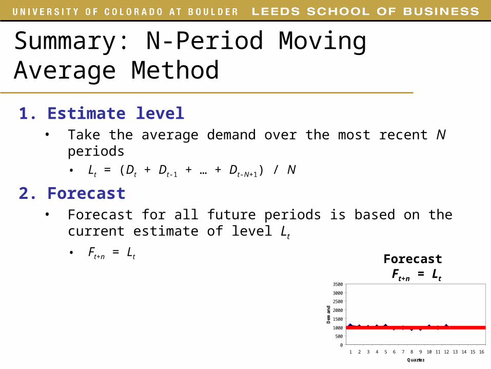
Summary: Winter’s Model (Trend and Seasonality Corrected Exp. Smoothing)1. Estimate level, trend, and seasonality

• The initial estimates of L0, T0, S1, S2, S3, and S4 are obtained from static forecasting procedure

• Revise the estimates for all periods using smoothing constants , and • Lt+1 = (Dt+1/St+1) + (1 – )*(Lt + Tt)

• Tt+1 = (Lt+1 – Lt) + (1 – )*Tt

• St+p+1 = (Dt+1/Lt+1) + (1 – )St+1

2. Forecast• Forecast for future periods is

• Ft+n = (Lt + nTt)*St+n

0

500

1000

1500

2000

2500

3000

3500

1 2 3 4 5 6 7 8 9 10 11 12 13 14 15 16

Quarter

Dem

and

Forecast Ft+n = (Lt + nTt)St+n

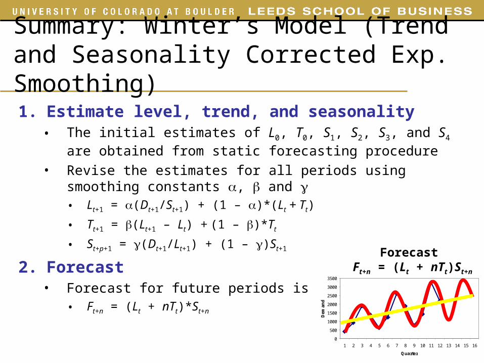
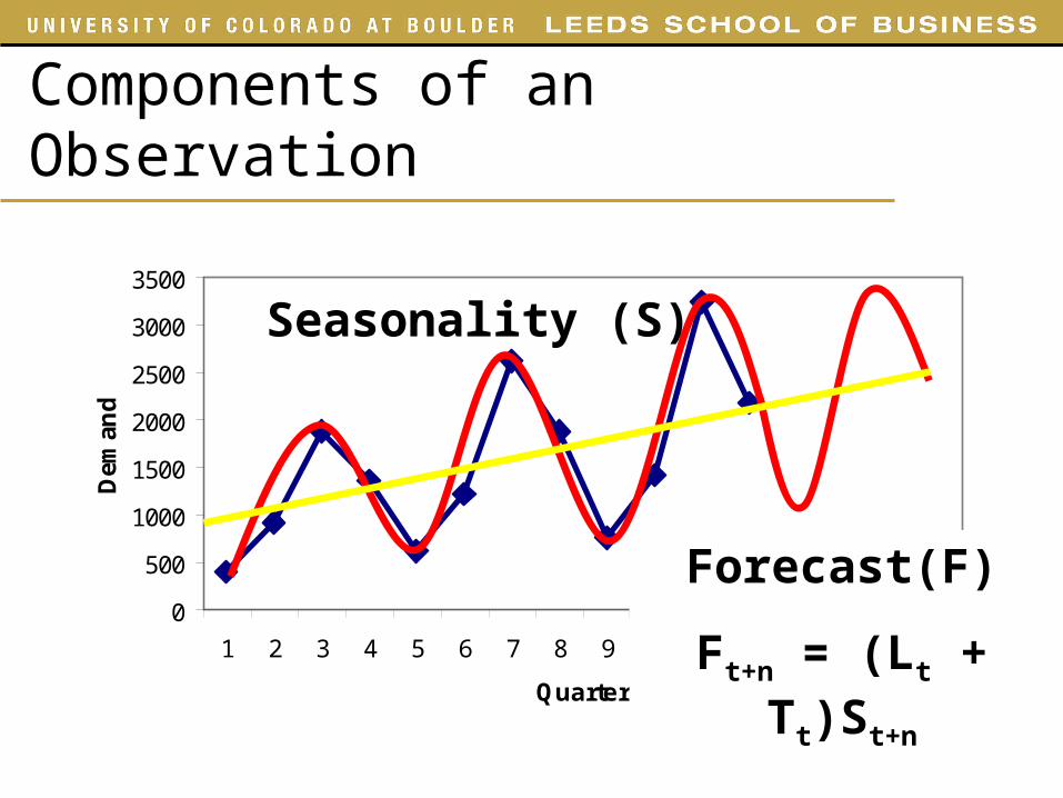
Components of an Observation

0

500

1000

1500

2000

2500

3000

3500

1 2 3 4 5 6 7 8 9 10 11 12 13 14 15 16

Quarter

Dem

and

Trend (T)

Forecast(F)

Ft+n = Lt + nTt

Holt’s method is appropriate when demand is assumed to have a level and a trend

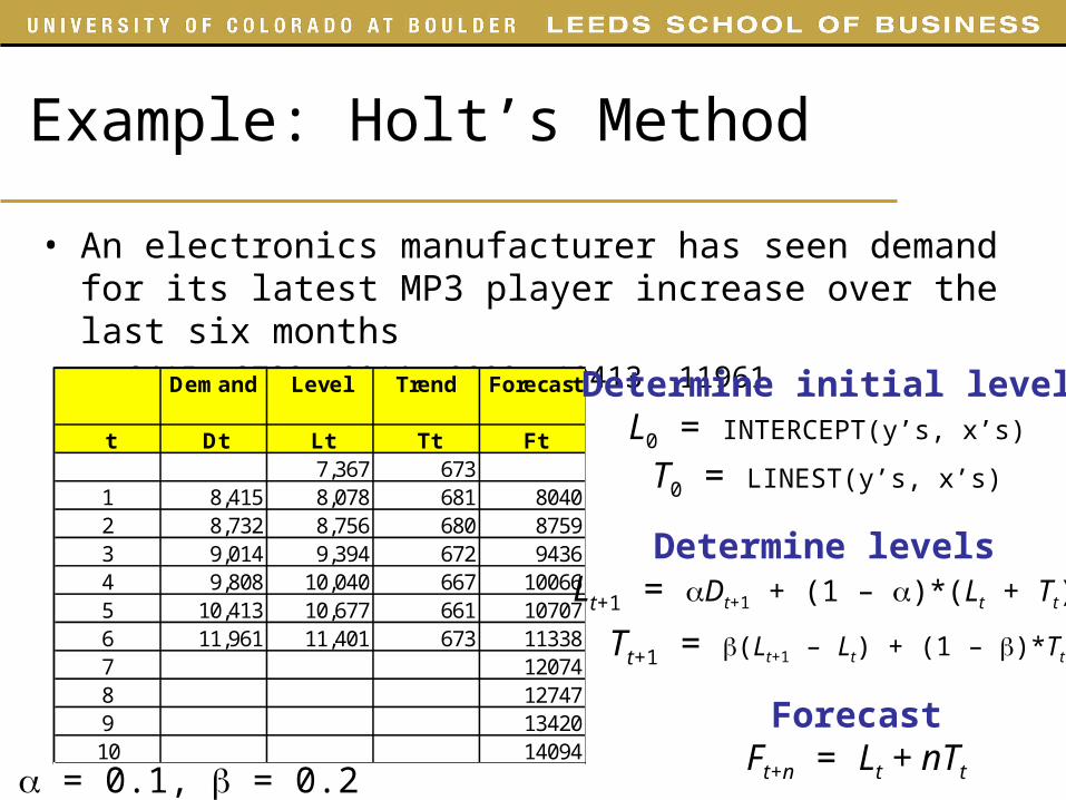
Example: Holt’s Method

• An electronics manufacturer has seen demand for its latest MP3 player increase over the last six months– 8415, 8732, 9014, 9808, 10413, 11961

Demand Level Trend Forecast

t Dt Lt Tt Ft

1 8,4152 8,7323 9,0144 9,8085 10,4136 11,96178910

Determine initial levelL0 = INTERCEPT(y’s, x’s)

T0 = LINEST(y’s, x’s)

Example: Holt’s Method

• An electronics manufacturer has seen demand for its latest MP3 player increase over the last six months– 8415, 8732, 9014, 9808, 10413, 11961

Demand Level Trend Forecast

t Dt Lt Tt Ft7,367 673

1 8,4152 8,7323 9,0144 9,8085 10,4136 11,96178910

Demand Level Trend Forecast

t Dt Lt Tt Ft7,367 673

1 8,415 8,078 6812 8,732 8,756 6803 9,014 9,394 6724 9,808 10,040 6675 10,413 10,677 6616 11,961 11,401 67378910

Demand Level Trend Forecast

t Dt Lt Tt Ft7,367 673

1 8,415 8,078 681 80402 8,732 8,756 680 87593 9,014 9,394 672 94364 9,808 10,040 667 100665 10,413 10,677 661 107076 11,961 11,401 673 113387 120748910

Demand Level Trend Forecast

t Dt Lt Tt Ft7,367 673

1 8,415 8,078 681 80402 8,732 8,756 680 87593 9,014 9,394 672 94364 9,808 10,040 667 100665 10,413 10,677 661 107076 11,961 11,401 673 113387 120748 127479 1342010 14094

Determine initial levelL0 = INTERCEPT(y’s, x’s)

T0 = LINEST(y’s, x’s)

Determine levelsLt+1 = Dt+1 + (1 – )*(Lt + Tt)

Tt+1 = (Lt+1 – Lt) + (1 – )*Tt

ForecastFt+n = Lt + nTt = 0.1, = 0.2

Example: Tahoe Salt

Example: Tahoe Salt

• Demand forecasting using Holt’s method

0

10,000

20,000

30,000

40,000

50,000

1 2 3 4 5 6 7 8 9 10 11 12 13 14 15 16

Quarter

Dem

and

Actual

Forecast (Holt)

Components of an Observation

0

500

1000

1500

2000

2500

3000

3500

1 2 3 4 5 6 7 8 9 10 11 12 13 14 15 16

Quarter

Dem

and

Seasonality (S)

Forecast(F)

Ft+n = (Lt + Tt)St+n

Example: Winter’s Model

• A theme park has seen the following attendance over the last eight quarters (in thousands)– 54, 87, 192, 130, 80, 124, 265, 171 Determine initial levels

L0 = From static forecast

T0 = From static forecast

Si,0 = From static forecast

ForecastFt+1 = (Lt + Tt)St+1

Determine levelsLt+1 = (Dt+1/St+1)+ (1 – )*(Lt + Tt)

Tt+1 = (Lt+1 – Lt) + (1 – )*Tt

St+p+1 = (Dt+1/Lt+1) + (1 – )*St+1

Demand Level Trend Seasonal ForecastFactor

t Dt L T Si Ft

1 542 873 1924 1305 806 1247 2658 171

Example: Tahoe Salt

Example: Tahoe Salt

• Demand forecast using Winter’s method

0

10,000

20,000

30,000

40,000

50,000

1 2 3 4 5 6 7 8 9 10 11 12 13 14 15 16

Quarter

Dem

and

Actual

Forecast (Winter)

Static Versus Adaptive Forecasting Methods

• Static– Dt: Actual demand

– L: Level– T: Trend– S: Seasonal factor

– Ft: Forecast

• Adaptive– Dt: Actual demand

– Lt: Level

– Tt: Trend

– St: Seasonal factor

– Ft: Forecast

Components of an Observation

0

500

1000

1500

2000

2500

3000

3500

1 2 3 4 5 6 7 8 9 10 11 12 13 14 15 16

Quarter

Dem

and

Seasonality (S)

Forecast(F)

Ft+n = (Lt + Tt)St+n

Example: Static Method

• A theme park has seen the following attendance over the last eight quarters (in thousands)– 54, 87, 192, 130, 80, 124, 265, 171

Determine initial levelL = INTERCEPT(y’s, x’s)

T = LINEST(y’s, x’s)

Determine deason. demandDt = L + Tt

Determine seasonal factorsSt = Dt / Dt

Determine seasonal factorsSi =AVG(St)Forecast

Ft = (L + T)Si

Demand Level Trend Deseason. Seasonal Seasonal ForecastDemand Factor Factor

t Dt L T Dt_bar Si_bar Si Ft

1 542 873 1924 1305 806 1247 2658 171

Demand Level Trend Deseason. Seasonal Seasonal ForecastDemand Factor Factor

t Dt L T Dt_bar Si_bar Si Ft59.3 17.3

1 542 873 1924 1305 806 1247 2658 171

Demand Level Trend Deseason. Seasonal Seasonal ForecastDemand Factor Factor

t Dt L T Dt_bar Si_bar Si Ft59.3 17.3

1 54 76.62 87 93.93 192 111.24 130 128.55 80 145.86 124 163.17 265 180.48 171 197.7

Demand Level Trend Deseason. Seasonal Seasonal ForecastDemand Factor Factor

t Dt L T Dt_bar Si_bar Si Ft59.3 17.3

1 54 76.6 0.702 87 93.9 0.933 192 111.2 1.734 130 128.5 1.015 80 145.8 0.556 124 163.1 0.767 265 180.4 1.478 171 197.7 0.86

Demand Level Trend Deseason. Seasonal Seasonal ForecastDemand Factor Factor

t Dt L T Dt_bar Si_bar Si Ft59.3 17.3

1 54 76.6 0.70 0.632 87 93.9 0.93 0.843 192 111.2 1.73 1.604 130 128.5 1.01 0.945 80 145.8 0.556 124 163.1 0.767 265 180.4 1.478 171 197.7 0.86

Demand Level Trend Deseason. Seasonal Seasonal ForecastDemand Factor Factor

t Dt L T Dt_bar Si_bar Si Ft59.3 17.3

1 54 76.6 0.70 0.63 48.02 87 93.9 0.93 0.84 79.23 192 111.2 1.73 1.60 177.74 130 128.5 1.01 0.94 120.65 80 145.8 0.55 91.46 124 163.1 0.76 137.67 265 180.4 1.47 288.28 171 197.7 0.86 185.5

Example: Tahoe Salt

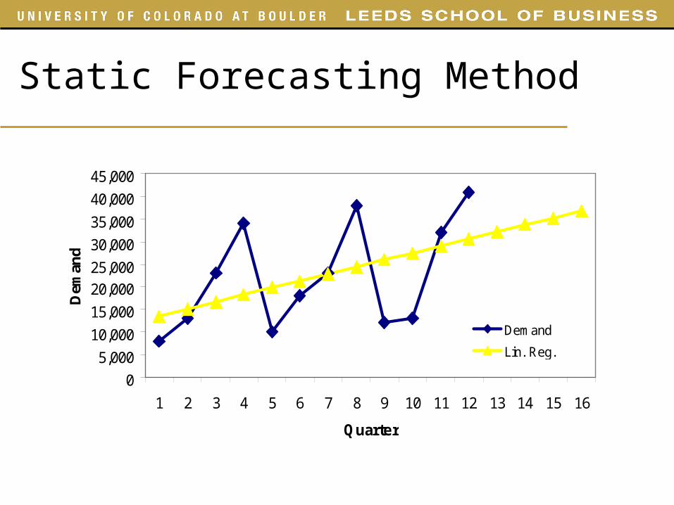
Static Forecasting Method

0

5,000

10,000

15,000

20,000

25,000

30,000

35,000

40,000

45,000

1 2 3 4 5 6 7 8 9 10 11 12 13 14 15 16

Quarter

Dem

and

Demand

0

5,000

10,000

15,000

20,000

25,000

30,000

35,000

40,000

45,000

1 2 3 4 5 6 7 8 9 10 11 12 13 14 15 16

Quarter

Dem

and

Demand

Lin. Reg.

Static Forecasting Method

• Deseasonalize demand– Demand that would have been observed in the

absence of seasonal fluctuations

• Periodicity p– The number of periods after which the seasonal cycle

repeats itself• 12 months in a year• 7 days in a week• 4 quarters in a year• 3 months in a quarter

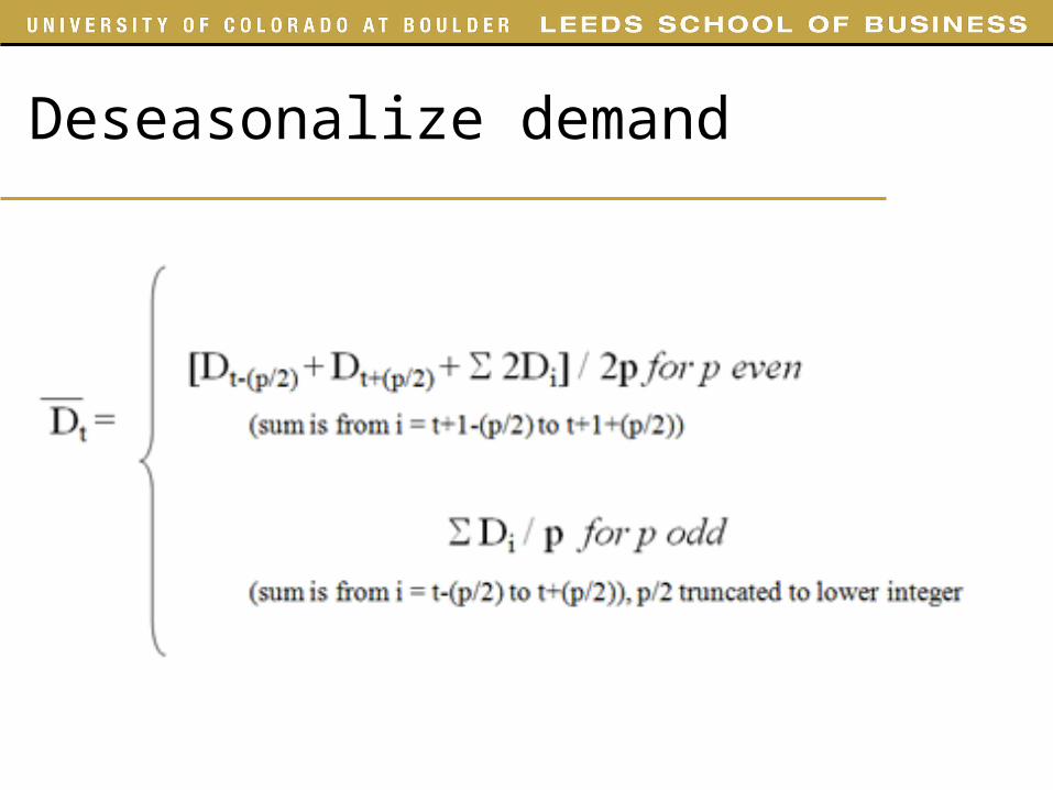
Deseasonalize demand

Deseasonalize demand

• Periodicity p is odd • Periodicity p is even

Demand Deseason.Demand

t Dt

1 8,0002 13,0003 23,000 19,7504 34,000 20,6255 10,000 21,2506 18,000 21,7507 23,000 22,5008 38,000 22,1259 12,000 22,62510 13,000 24,12511 32,00012 41,000

Demand Deseason.Demand

t Dt

1 8,0002 13,000 14,6673 23,000 15,3334 10,000 17,0005 18,000 17,0006 23,000 17,6677 12,000 16,0008 13,000 19,0009 32,000101112

Example: Tahoe Salt

Static Forecasting Method

0

5,000

10,000

15,000

20,000

25,000

30,000

35,000

40,000

45,000

1 2 3 4 5 6 7 8 9 10 11 12 13 14 15 16

Quarter

Dem

and

Demand

Deseason.

0

5,000

10,000

15,000

20,000

25,000

30,000

35,000

40,000

45,000

1 2 3 4 5 6 7 8 9 10 11 12 13 14 15 16

Quarter

Dem

and

Demand

Deseason.

Deseason. Lin. Reg.

Example: Tahoe Salt

• Demand forecast using Static forecasting method

0

10,000

20,000

30,000

40,000

50,000

1 2 3 4 5 6 7 8 9 10 11 12 13 14 15 16

Quarter

Dem

and

Actual

Forecast (Static)

Summary: Static Forecasting Method

1. Estimate level and trend• Deseasonalize the demand data• Estimate level L and trend T using linear regression

• Obtain deasonalized demand Dt

2. Estimate seasonal factors• Estimate seasonal factors for each period St = Dt /Dt

• Obtain seasonal factors Si = AVG(St) such that t is the same season as i

3. Forecast• Forecast for future periods is

• Ft+n = (L + nT)*St+n

0

500

1000

1500

2000

2500

3000

3500

1 2 3 4 5 6 7 8 9 10 11 12 13 14 15 16

Quarter

Dem

and

Forecast Ft+n = (L + nT)St+n

Forecast Forecast error

Time Series Forecasting

Observed demand =

Systematic component + Random component

L Level (current deseasonalized demand)T Trend (growth or decline in demand)S Seasonality (predictable seasonal fluctuation)

The goal of any forecasting method is to predict the systematic component (Forecast) of demand and measure the size and

variability of the random component (Forecast error)

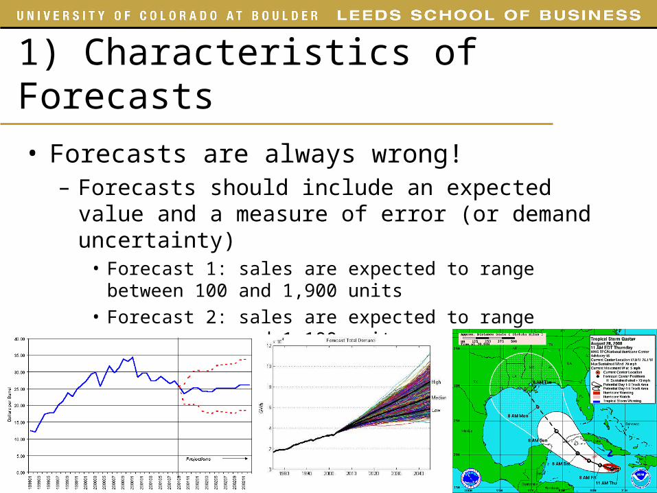
1) Characteristics of Forecasts

• Forecasts are always wrong!– Forecasts should include an expected value and a

measure of error (or demand uncertainty)• Forecast 1: sales are expected to range between 100

and 1,900 units• Forecast 2: sales are expected to range between 900

and 1,100 units

Examples

8000

9000

10000

1 2 3 4 5 6 7 8 9 10 11 12

Demand

Forecast

0

10000

20000

30000

40000

1 2 3 4 5 6 7 8 9 10 11 12

Demand

Forecast

0

10000

20000

30000

40000

50000

1 2 3 4 5 6 7 8 9 10 11 12

Demand

Forecast

800000

900000

1000000

1 2 3 4 5 6 7 8 9 10 11 12

Demand

Forecast

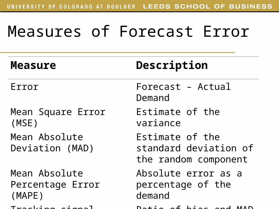
Measures of Forecast Error

Measure Description

Error Forecast – Actual Demand

Mean Square Error (MSE) Estimate of the variance

Mean Absolute Deviation (MAD)

Estimate of the standard deviation of the random component

Mean Absolute Percentage Error (MAPE)

Absolute error as a percentage of the demand

Tracking signal Ratio of bias and MAD