Supply Chain Location Decisions Chapter 11 Copyright ©2013 Pearson Education, Inc. publishing as Prentice Hall 11- 01.

Supply Chain Location DecisionsChapter 11

Copyright ©2013 Pearson Education, Inc. publishing as Prentice Hall 11- 01

What is a Facility Location?

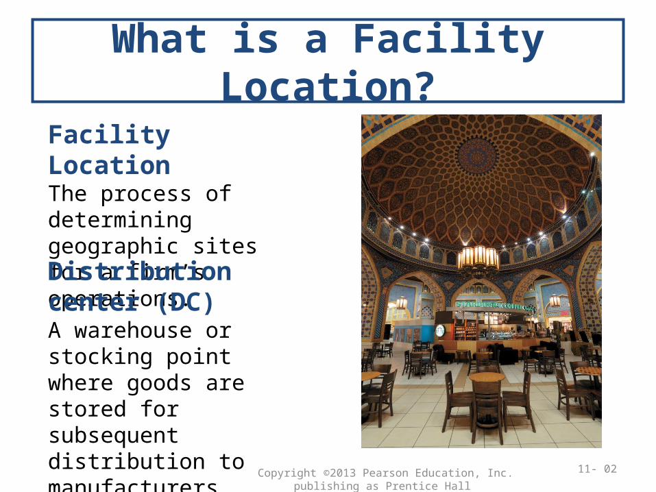
Facility LocationThe process of determining geographic sites for a firm’s operations.

11- 02Copyright ©2013 Pearson Education, Inc. publishing as Prentice Hall

Distribution center (DC)A warehouse or stocking point where goods are stored for subsequent distribution to manufacturers, wholesalers, retailers, and customers.

Location Decisions

• Factors affecting location decisions

– Sensitive to location

– High impact on the company’s ability to meet its goals

11 - 03Copyright ©2013 Pearson Education, Inc. publishing as Prentice Hall

Location Decisions

• Dominant factors in manufacturing– Favorable labor climate

– Proximity to markets

– Impact on Environment

– Quality of life

– Proximity to suppliers and resources

– Proximity to the parent company’s facilities

– Utilities, taxes, and real estate costs

– Other factorsCopyright ©2013 Pearson Education, Inc. publishing as Prentice Hall 11 - 04

Location Decisions

• Dominant factors in services– Impact of location on sales and customer

satisfaction

– Proximity to customers

– Transportation costs and proximity to markets

– Location of competitors

– Site-specific factors


What is a GIS?

GIS – Geographical Information System

A system of computer software, hardware, and data that the firm’s personnel can use to manipulate, analyze, and present information relevant to a location decision.

11- 06Copyright ©2013 Pearson Education, Inc. publishing as Prentice Hall

Locating a Single Facility

• Expand onsite, build another facility, or relocate to another site

– Onsite expansion

– Building a new plant or moving to a new retail or office space

• Comparing several sites


Selecting a New Facility

Step 1: Identify the important location factors and categorize them as dominant or secondary.

Step 2: Consider alternative regions; then narrow to alternative communities and finally specific sites.

Step 3: Collect data on the alternatives.

Step 4: Analyze the data collected, beginning with the quantitative factors.

Step 5: Bring the qualitative factors pertaining to each site into the evaluation.


A new medical facility, Health-Watch, is to be located in Erie, Pennsylvania. The following table shows the location factors, weights, and scores (1 = poor, 5 = excellent) for one potential site. The weights in this case add up to 100 percent. A weighted score (WS) will be calculated for each site. What is the WS for this site?

Example 11.1

Location Factor Weight ScoreTotal patient miles per month 25 4Facility utilization 20 3Average time per emergency trip 20 3Expressway accessibility 15 4Land and construction costs 10 1Employee preferences 10 5


The WS for this particular site is calculated by multiplying each factor’s weight by its score and adding the results:

Example 11.1Location Factor Weight ScoreTotal patient miles per month 25 4Facility utilization 20 3Average time per emergency trip 20 3

Expressway accessibility 15 4Land and construction costs 10 1Employee preferences 10 5

WS = (25 4) + (20 3) + (20 3) + (15 4) + (10 1) + (10 5)= 100 + 60 + 60 + 60 + 10 + 50= 340

The total WS of 340 can be compared with the total weighted scores for other sites being evaluated.


Applying the Load-Distance (ld) Method

• Identify and compare candidate locations

– Like weighted-distance method

– Select a location that minimizes the sum of the loads multiplied by the distance the load travels

– Time may be used instead of distance


Applying the Load-Distance (ld) Method

• Calculating a load-distance score– Varies by industry

– Use the actual distance to calculate ld score

– Use rectangular or Euclidean distances

– Different measures for distance

– Find one acceptable facility location that minimizes the ld score

• Formula for the ld scoreld = lidii


Application 11.2

What is the distance between (20, 10) and (80, 60)?

Euclidean distance:

dAB = (xA – xB)2 + (yA – yB)2 = (20 – 80)2 + (10 – 60)2 = 78.1

Rectilinear distance:

dAB = |xA – xB| + |yA – yB| = |20 – 80| + |10 – 60| = 110


Application 11.3Management is investigating which location would be best to position its new plant relative to two suppliers (located in Cleveland and Toledo) and three market areas (represented by Cincinnati, Dayton, and Lima). Management has limited the search for this plant to those five locations. The following information has been collected. Which is best, assuming rectilinear distance?

Location x,y coordinates Trips/year

Cincinnati (11,6) 15

Dayton (6,10) 20

Cleveland (14,12) 30

Toledo (9,12) 25

Lima (13,8) 40 11 - 14Copyright ©2013 Pearson Education, Inc. publishing as Prentice Hall

Application 11.3Location x,y

coordinates Trips/year

Cincinnati (11,6) 15Dayton (6,10) 20

Cleveland (14,12) 30Toledo (9,12) 25Lima (13,8) 40

15(9) + 20(0) + 30(10) + 25(5) + 40(9) = 92015(9) + 20(10) + 30(0) + 25(5) + 40(5) = 66015(8) + 20(5) + 30(5) + 25(0) + 40(8) = 690

15(4) + 20(9) + 30(5) + 25(8) + 40(0) = 590

15(0) + 20(9) + 30(9) + 25(8) + 40(4) = 810Cincinnati = Dayton =

Cleveland = Toledo =

Lima =


Center of Gravity Method• A good starting point

– Find x coordinate, x*, by multiplying each point’s x coordinate by its load (lt), summing these products li xi, and dividing by li

– The center of gravity’s y coordinate y* found the same way

– Generally not the optimal location

x* =li xi

li

i

i

y* =li yi

li

i

i


Application 11.4A firm wishes to find a central location for its service. Business forecasts indicate travel from the central location to New York City on 20 occasions per year. Similarly, there will be 15 trips to Boston, and 30 trips to New Orleans. The x, y-coordinates are (11.0, 8.5) for New York, (12.0, 9.5) for Boston, and (4.0, 1.5) for New Orleans. What is the center of gravity of the three demand points?

x* = =li xi

li

i

i

y* = =li yi

li

i

i

[(20 11) + (15 12) + (30 4)](20 + 15 + 30)

= 8.0

[(20 8.5) + (15 9.5) + (30 1.5)](20 + 15 + 30)

= 5.5


Using Break-Even Analysis

• Compare location alternatives on the basis of quantitative factors expressed in total costs

– Determine the variable costs and fixed costs for each site

– Plot total cost lines– Identify the approximate ranges for which each

location has lowest cost– Solve algebraically for break-even points over the

relevant ranges


Example 11.3An operations manager narrowed the search for a new facility location to four communities. The annual fixed costs (land, property taxes, insurance, equipment, and buildings) and the variable costs (labor, materials, transportation, and variable overhead) are as follows:

Community Fixed Costs per Year Variable Costs per Unit

A $150,000 $62

B $300,000 $38

C $500,000 $24

D $600,000 $30


Example 11.3

Step 1:Plot the total cost curves for all the communities on a single graph. Identify on the graph the approximate range over which each community provides the lowest cost.

Step 2:Using break-even analysis, calculate the break-even quantities over the relevant ranges. If the expected demand is 15,000 units per year, what is the best location?


Example 11.3To plot a community’s total cost line, let us first compute the total cost for two output levels: Q = 0 and Q = 20,000 units per year. For the Q = 0 level, the total cost is simply the fixed costs. For the Q = 20,000 level, the total cost (fixed plus variable costs) is as follows:

Community Fixed CostsVariable Costs

(Cost per Unit)(No. of Units)Total Cost

(Fixed + Variable)

A $150,000

B $300,000

C $500,000

D $600,000


Example 11.3

$62(20,000) = $1,240,000 $1,390,000

Community Fixed CostsVariable Costs

(Cost per Unit)(No. of Units)Total Cost

(Fixed + Variable)

A $150,000

B $300,000

C $500,000

D $600,000

$38(20,000) = $760,000 $1,060,000

$24(20,000) = $480,000 $980,000

$30(20,000) = $600,000 $1,200,000


To plot a community’s total cost line, let us first compute the total cost for two output levels: Q = 0 and Q = 20,000 units per year. For the Q = 0 level, the total cost is simply the fixed costs. For the Q = 20,000 level, the total cost (fixed plus variable costs) is as follows:

A best B best C best

Example 11.3The figure shows the graph of the total cost lines.

| | | | | | | | | | | |

0 2 4 6 8 10 12 14 16 18 20 22

1,600 –

1,400 –

1,200 –

1,000 –

800 –

600 –

400 –

200 –

–

An

nu

al c

ost

(th

ou

san

ds

of

do

llar

s)

Q (thousands of units)

A

B

C

D

6.25 14.3

Break-even point

Break-even point

(20, 980)

(20, 1,390)

(20, 1,200)

(20, 1,060)• A is best for low volumes• B for intermediate

volumes• C for high volumes. • We should no longer

consider community D, because both its fixed and its variable costs are higher than community C’s.


Example 11.3

(A) (B)$150,000 + $62Q = $300,000 + $38QQ = 6,250 units

The break-even quantity between B and C lies at the end of the range over which B is best and the beginning of the final range where C is best.

(B) (C)$300,000 + $38Q = $500,000 + $24Q

Q = 14,286 units 11 - 24Copyright ©2013 Pearson Education, Inc. publishing as Prentice Hall

The break-even quantity between A and B lies at the end of the first range, where A is best, and the beginning of the second range, where B is best.

Example 11.3

(A) (B)$150,000 + $62Q = $300,000 + $38QQ = 6,250 units

The break-even quantity between B and C lies at the end of the range over which B is best and the beginning of the final range where C is best.

(B) (C)$300,000 + $38Q = $500,000 + $24QQ = 14,286 units


The break-even quantity between A and B lies at the end of the first range, where A is best, and the beginning of the second range, where B is best.

No other break-even quantities are needed. The break-even point between A and C lies above the shaded area, which does not mark either the start or the end of one of the three relevant ranges.

Locating a facility within a Supply Chain Network

• When a firm with a network of existing facilities plans a new facility, one of two conditions exists

– Facilities operate independently

– Facilities interact


Supply Chain Location Decisions Chapter 11 Copyright ©2013 Pearson Education, Inc. publishing as Prentice Hall 11- 01.

Documents

facility location

location decisions factors

factors copyright

prentice hall slide

pearson education

important location factors

location decisions sensitive

location high impact