Supply Chain Disruptions and the Role of Information ...

Supply Chain Disruptions and the Role of Information Asymmetry

CitationSchmidt, William. 2013. Supply Chain Disruptions and the Role of Information Asymmetry. Doctoral dissertation, Harvard Business School.

Permanent linkhttps://nrs.harvard.edu/URN-3:HUL.INSTREPOS:37367796

Terms of UseThis article was downloaded from Harvard University’s DASH repository, and is made available under the terms and conditions applicable to Other Posted Material, as set forth at http://nrs.harvard.edu/urn-3:HUL.InstRepos:dash.current.terms-of-use#LAA

Share Your StoryThe Harvard community has made this article openly available.Please share how this access benefits you. Submit a story .

Accessibility

Supply Chain Disruptions and the Role of InformationAsymmetry

W S

T T O M U

D B A

O M

H B SB , M

M

© - W SA .

Supply Chain Disruptions and the Role of Information Asymmetry

A

My research examines how rm operational decisions in uence and are in uenced by rm value. In

particular, I focus on these relationships in the context of low probability, high impact disruptions. Over

the last several years, companies have faced rising levels of risk and volatility that affect their operations

and supply chains. Some recent examples include the unrest in the Middle East, global nancial shocks,

volcano-related transportation disruptions in Europe, oil price volatility, and natural disasters. As a result,

supply chain executives increasingly have a dual mission – to systematically address extreme risks such as

hurricanes, epidemics, earthquakes or port closings, and to manage conventional risks, such as forecast

errors, sourcing problems, and transportation breakdowns. In an environment where extreme risks are

difficult to predict and have a variable impact on the rm, there is no panacea that will fully insulate the

company and its operations. With my research I intend to provide rms with meaningful insights on how

to manage this uncertainty by measuring and mitigating the level of risk in their operations. My

dissertation focuses on one important aspect of this issue – how information asymmetry between the rm

and its investors may lead managers within the rm to take actions which increase rather than decrease

the rm’s exposure to low probability, high impact disruptions.

In the rst chapter, I examine the role of information asymmetry in inducing managerial decisions that

contribute to supply chain disruptions. I use signaling game theory to develop a stylized model of a

capacity investment decision by the rm’s management. I integrate the Newsvendor Model, a canonical

capacity planning tool, into the signaling game in order to tie the results directly to common operations

management decision se ings. In the model, the manager has private information about the rm’s

operations and may take a suboptimal capacity decision in order to signal her private information to an

uninformed investor, and thereby in uence the short-term stock price of the rm. Distinguishing features

of the analysis are that: (i) I allow the capacity decision to be either in discrete increments or continuous,

and (ii) I allow beliefs to be re ned based on either the Undefeated re nement or the Intuitive Criterion

iii

re nement. Previous research has shown that under continuous decision choices and the Intuitive

Criterion re nement, information asymmetry gives rise to the least cost separating equilibrium, in which

a low quality rm chooses its optimal capacity and a high quality rm over-invests in order to signal its

quality to investors. I build on this research by showing the existence of pooling outcomes in which low

quality rms over-invest and high quality rms under-invest so as to provide identical signals to investors.

e pooling equilibrium is practically appealing because it yields a Pareto improvement compared to the

least cost separating equilibrium. Such an outcome makes clear, however, that managers may knowingly

under-invest in capacity.

If management engages in such myopic decision-making, then some portion of supply chain

disruptions may be self-in icted. is has direct implications for how to effectively mitigate disruptions.

For instance, proper consideration should be given to the development of managerial incentive schemes

to ensure they aren’t inducing such undesirable outcomes. To gain some insight on when such myopic

decision making can be expected, I run a numerical analysis consisting of approximately . million

scenarios based on the inputs in our model. Feeding the results of this numerical analysis into an

empirical model, I show that the parameters of the Newsvendor Model have a signi cant in uence on the

likelihood of myopic decision making, and that the magnitude and direction of this in uence is highly

sensitive to which assumptions are relaxed. Finally, I provide evidence from executive interviews that

support the results of our model.

is analysis is important because it provides a tractable model to analyze myopic behavior in a

common operations management se ing. It is relevant to my research because it shows that supply chain

disruptions can be traced to management’s purposeful actions, and the circumstances under which such

behavior should be expected. It is also surprising because it reveals that the outcomes from the model are

highly sensitive to two assumptions which have been widely employed in the literature – capacity choices

with continuous support and the application of the Intuitive Criterion re nement.

In the second chapter, I present the results of a controlled experiment that analyzes whether the

Intuitive Criterion re nement or the Undefeated re nement is a be er predictor of decisions made under

iv

information asymmetry. Recall that chapter considers the implications of both discrete capacity

decisions and re ning the participants’ beliefs using the Undefeated re nement as opposed to the

Intuitive Criterion re nement. While using discrete support for capacity choices is well established in the

operations literature, the use of the Undefeated re nement has received less a ention. Deciding which

re nement to employ is central in analyses involving be er informed decision makers that are called upon

to make choices which may provide a costly yet informative signal to less informed parties. A challenge in

such se ings is how to handle the plethora of equilibrium outcomes that are o en produced from the

analysis. Researchers address this issue by using belief re nements, which pare the set of equilibrium

outcomes by making assumptions on how the players in the game form their beliefs.

Both the Undefeated and Intuitive Criterion re nements are theoretically sound, and researchers are

justi ed in adopting either approach on those grounds. Our experiment, however, is the rst direct

empirical evidence of whether individuals make decisions which are consistent with the Undefeated

re nement compared to the Intuitive Criterion re nement. I examine this issue in a se ing central to

operations management – a capacity investment decision. I nd that the Undefeated re nement is a much

be er predictor of individual choices and that these results stand up when greater complexity is added to

the game. e proportion of subjects making choices consistent with the Intuitive Criterion, however, is

relatively low and reduces further as the complexity of the game increases.

A common criticism of complex experiments is that the subjects may not understand the game, and

this lack of understanding governs their behavior. I address this by running practice rounds to acclimate

the subjects to the game, having subjects change roles during the game, and requiring subjects to de ne

their strategies before playing each round in the game. I also ask subjects to rate their understanding of the

game before they are paid. I show that individuals making decisions which are consistent with the

Undefeated re nement report a higher understanding of the game and earn more money from the game.

ese results provide strong support that decisions are made consistent with the Undefeated

re nement rather than the Intuitive Criterion re nement. is is surprising because the Undefeated

re nement has not been applied in our eld, and yet it is more predictive of actual decision making. It is

v

also important because, as I show in both chapters and , the results generated by the Undefeated

re nement can o en be materially different compared to those generated by the Intuitive Criterion

re nement. For instance, the Undefeated re nement is far more likely to predict a pooling equilibrium

such that managers at superior rms commit to lower capacity levels while managers at inferior rms

commit to higher capacity levels. is ties to the theme of my research because it demonstrates that

superior rms can expose themselves to potential disruption by building out less than the optimal level of

capacity.

In the nal chapter, I examine whether managers exercise signi cant discretion in disclosing supply

chain disruptions to investors. A major challenge in empirical research on supply chain disruptions is the

possibility that selection issues prevent the identi cation of material, disruptive events. It is not clear

whether managerial disclosure of such events is in uenced by the expected impact of the event on the

rm’s share price, nor is it clear whether this impact would differ if managers were more forthcoming. I

empirically examine these issues using a sample of over disruption announcements collected from

company press releases. I take advantage of an exogenous regulatory shock, the enforcement date of new

corporate disclosure rules, to identify whether managers were previously exercising signi cant discretion

in deciding whether or not to reveal material disruptions affecting the rm. I nd that a er the regulatory

change, managers disclosed far more material disruptive events, indicating that they had previously been

suppressing their release. I also nd that there is a signi cant amelioration in the average impact of

disruptions on rm value a er managers improve their disclosure practices. Finally, I show that

disruptions a ributed to the rm’s internal operations are far more damaging to rm value than those

a ributed to environmental factors, and this difference persists a er disclosure is improved.

e impact of disruptions on rm value can vary widely. My ndings are important for managers and

investors alike because they help identify the types of disruptions and the rm characteristics that

contribute disproportionately to the most damaging announcements. Countermeasures to mitigate the

risk of disruptions have a cost, and insights into the types of disruptions that represent the greatest risk to

company value will help managers assess whether the company is investing appropriately to mitigate the

vi

most material risks.

vii

Contents

S P I I N M. Introduction . . . . . . . . . . . . . . . . . . . . . . . . . . . . . . . . . . . . . . . .. Literature Review . . . . . . . . . . . . . . . . . . . . . . . . . . . . . . . . . . . . . .. Model Setup . . . . . . . . . . . . . . . . . . . . . . . . . . . . . . . . . . . . . . . .. Existence of Pooling and Separating PBE . . . . . . . . . . . . . . . . . . . . . . . . . .. Re nement of Out-of-Equilibrium Beliefs . . . . . . . . . . . . . . . . . . . . . . . . .. Numerical Analysis . . . . . . . . . . . . . . . . . . . . . . . . . . . . . . . . . . . . .. Managerial Implications and Discussion . . . . . . . . . . . . . . . . . . . . . . . . . .

T G P P : E D M U I A -

. Introduction . . . . . . . . . . . . . . . . . . . . . . . . . . . . . . . . . . . . . . . .

. Literature Review . . . . . . . . . . . . . . . . . . . . . . . . . . . . . . . . . . . . . .

. eory . . . . . . . . . . . . . . . . . . . . . . . . . . . . . . . . . . . . . . . . . . .

. Data . . . . . . . . . . . . . . . . . . . . . . . . . . . . . . . . . . . . . . . . . . . . .

. Results . . . . . . . . . . . . . . . . . . . . . . . . . . . . . . . . . . . . . . . . . . .

. Implications and Conclusions . . . . . . . . . . . . . . . . . . . . . . . . . . . . . . .

. Appendix . . . . . . . . . . . . . . . . . . . . . . . . . . . . . . . . . . . . . . . . . .

M D M ’ R S C D. Introduction . . . . . . . . . . . . . . . . . . . . . . . . . . . . . . . . . . . . . . . .. Literature Review . . . . . . . . . . . . . . . . . . . . . . . . . . . . . . . . . . . . . .. eory and Hypotheses . . . . . . . . . . . . . . . . . . . . . . . . . . . . . . . . . .. Data and Empirical Models . . . . . . . . . . . . . . . . . . . . . . . . . . . . . . . . .. Results . . . . . . . . . . . . . . . . . . . . . . . . . . . . . . . . . . . . . . . . . . .

viii

. Limitations and Extensions . . . . . . . . . . . . . . . . . . . . . . . . . . . . . . . . .

. Discussion and Managerial Implications . . . . . . . . . . . . . . . . . . . . . . . . . .

R

ix

Author List

e following authors contributed to Chapter : Vishal Gaur (Cornell University), Richard Lai, andAnanth Raman (Harvard Business School).

e following authors contributed to Chapter : Ryan Buell (Harvard Business School).e following authors contributed to Chapter : Ananth Raman (Harvard Business School).

x

Listing of gures

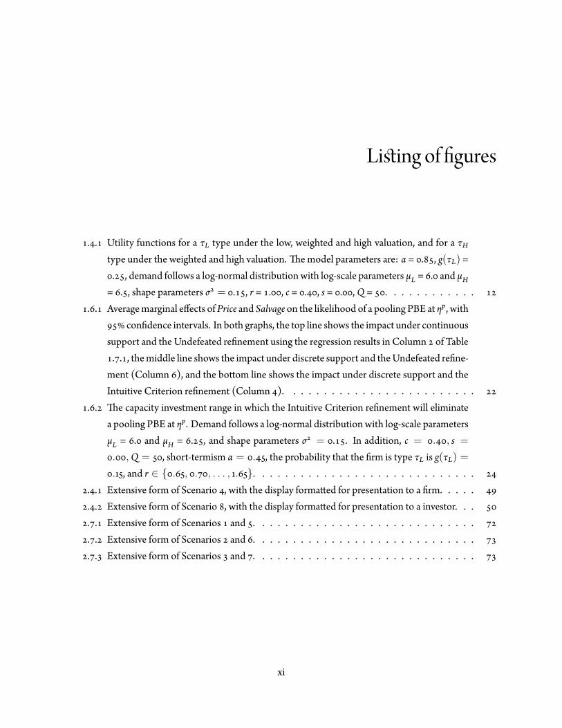
. . Utility functions for a τL type under the low, weighted and high valuation, and for a τHtype under the weighted and high valuation. e model parameters are: α = . , g(τL) =. , demand follows a log-normal distribution with log-scale parameters μL = . and μH

= . , shape parameters σ = . , r = . , c = . , s = . ,Q = . . . . . . . . . . . .. . Averagemarginal effects ofPrice and Salvage on the likelihood of a pooling PBE at ηp, with

con dence intervals. In both graphs, the top line shows the impact under continuoussupport and the Undefeated re nement using the regression results in Column of Table. . , themiddle line shows the impact under discrete support and theUndefeated re ne-

ment (Column ), and the bo om line shows the impact under discrete support and theIntuitive Criterion re nement (Column ). . . . . . . . . . . . . . . . . . . . . . . . .

. . e capacity investment range in which the Intuitive Criterion re nement will eliminatea pooling PBE at ηp. Demand follows a log-normal distribution with log-scale parametersμL = . and μH = . , and shape parameters σ = . . In addition, c = . , s =

. ,Q = , short-termism α = . , the probability that the rm is type τL is g(τL) =

. , and r ∈ { . , . , . . . , . }. . . . . . . . . . . . . . . . . . . . . . . . . . . . .. . Extensive form of Scenario , with the display forma ed for presentation to a rm. . . . .. . Extensive form of Scenario , with the display forma ed for presentation to a investor. . .. . Extensive form of Scenarios and . . . . . . . . . . . . . . . . . . . . . . . . . . . . .. . Extensive form of Scenarios and . . . . . . . . . . . . . . . . . . . . . . . . . . . . .. . Extensive form of Scenarios and . . . . . . . . . . . . . . . . . . . . . . . . . . . . .

xi

T , M . ILY, IWY, INY. A . K , HH B .

xii

Acknowledgments

I am grateful the the support, encouragement and guidance of my dissertation commi ee – AnanthRaman, Vishal Gaur, Mike Toffel, and Belen Villalonga. All of them contributed to my development anddirectly to research that is either in this dissertation or that will be a part of my early scholarship. I am alsograteful for all of the other collaborators and co-authors that I have been fortunate to work with, notablyAbigail Allen, Xiang Ao, Ryan Buell, Fern Jira, David Simchi-Levi, Bill Simpson, and Yehua Wei.

xiii

1Signaling to Partially Informed Investors in the

NewsvendorModel

. I

We investigate the effect on a rm’s capacity decisions of short-term objectives (short-termism) andasymmetric information between the rm and its equity holders. Managers may exhibit short-termism fora variety of reasons, including a desire to raise capital in a secondary offering (Stein ), to preventtakeovers (Stein ), or to burnish their reputation and careers (Holmström , Narayanan ).Although myopic decision making is decried as damaging the long-term value and competitiveness ofrms, it is widely acknowledged to occur. For example, Barton ( ) argues that the “mania over

quarterly earnings consumes extraordinary amounts of senior [managers’] time and a ention,” andexpresses dismay at “quarterly capitalism” (in which rms are unduly in uenced by short-term marketpressures). Rappaport ( ) acknowledges that “[t]o meet Wall Street expectations, managers makedecisions to increase short-term earnings – even at the expense of long-term shareholder value.” In asurvey of over nancial executives, Graham et al. ( ) nd that over would give up economicvalue in order to hit a short-term earnings target and would defer initiating a project with a very

positive net present value.is phenomenon is important to operations management because managers generally prefer

operational manipulations over accounting manipulations to meet performance benchmarks (Bruns andMerchant , Graham et al. ). Furthermore, evidence of myopic decision making is found in manyoperational se ings, including manipulating inventory levels ( omas and Zhang ), modifyingproduction schedules (Roychowdhury ), and postponing or eliminating maintenance, new projects,and R&D expenditures (Bushee , Roychowdhury ). Other recent empirical studies provideevidence that such behaviour harms long term performance (Cohen and Zarowin , Holden andLundstrum , Zhao et al. ).

Prior theoretical research in economics and operations has shown that, under standard assumptionscommonly used in the signaling game literature, the resulting unique perfect Bayesian equilibrium (PBE)is the least cost separating PBE in which a high quality rm over-invests in capacity compared to itslong-term optimal choice in order to signal its type to the market, whereas a low quality rm investsoptimally (Bebchuk and Stole , Lai et al. ). Our paper analyzes a signaling game between amanager of a rm and an equity holder of the rm. e rm can be one of two types with respect to itsdemand distribution - a low type or a high type. e type or quality of the rm is revealed to the managerbut not to the equity holder due to information asymmetry between them. e manager has short-termobjectives tied to the current stock price of the rm and makes a capacity investment decision using thenewsvendor model. e equity holder uses the manager’s capacity decision as a signal of the quality of therm and determines its stock price. We use this model to (i) identify conditions in which the rm

over-invests or under-invests in capacity compared to its optimal long term solution, and (ii) evaluate therole of the newsvendor model parameters in affecting the type of equilibrium and the level of investment.

Our contribution is to build on the existing research by considering two alternative assumptions. First,we allow the rm’s capacity decision to be discrete. Discreteness is a common characteristic of operationaldecisions, such as in sourcing, production and distribution, due to the use of integer-capacitated resources(Nahmias , p. ). Second, we examine the impact of re ning out-of-equilibrium (OOE) beliefsusing the Undefeated re nement. We do so in order to address known concerns about the IntuitiveCriterion, including that a high quality rm is presumed to choose the separating capacity investment atall costs even if the probability that it is a low quality rm approaches zero (Bolton and Dewatripont ,Kreps and Sobel ), the equity holder’s beliefs are not fully updated by the application of the IntuitiveCriterion (Mailath et al. , Salanie ), and the Intuitive Criterion may actually eliminate all PBE inthe game, leaving a model with no predictive power. ese points are discussed in Section . . .

We show the existence of pooling PBE, including situations in which a low type rm over-invests and ahigh type rm under-invests, when either or both of the above assumptions are relaxed. First, we show

that when the capacity investment choice is discrete, ( ) pooling PBE exist, ( ) in some cases separatingPBE do not exist at all, and ( ) in many cases, pooling PBE survive the Intuitive Criterion re nement.Second, when the Undefeated re nement is applied, we show that ( ) if one or more pooling PBE existthen at least one survives the Undefeated re nement, and ( ) if more than one PBE survives theUndefeated re nement, there is a unique lexicographically maximum sequential equilibrium (LMSE)from this set of PBE. In other words, the alternative re nement process predicts the existence of a uniquepooling PBE in identical situations in which the Intuitive Criterion re nement predicts the least costseparating PBE. erefore, it becomes important to examine the validity of differing predictions of thesemethods. A rich set of outcomes emerges from our model, such as a high quality rm under-invests whilea low quality rm invests optimally, a high quality rm under-invests while a low quality rm over-invests,both high and low quality rm types invest optimally, a high quality rm invests optimally while a lowquality rm over-invests, and a high quality rm over-invests while a low-quality rm invests optimally.

One limitation of our paper is that discrete support for the decision variable and the inequalities in thesignaling game framework prevent us from ge ing a closed form solution or comparative statics. Despitethis, our paper makes a valuable contribution because discrete choices are important in operationsmanagement and we are able to show that they produce a different equilibrium result. We examine ourtheoretical results through an exhaustive numerical analysis and evidence from practitioners. Ournumerical analysis shows that the existence of a pooling PBE is not a pathological phenomenon.Depending on which combination of assumptions are relaxed, a pooling PBE uniquely survivesre nement in to of the examined scenarios. e numerical analysis enhances the predictions ofthe theoretical model by showing that there is a sharp difference between the outcomes from the twocompeting re nements. We con rm the reasonableness of our results in practical se ings throughinterviews with executives. Our interview with the current Chairman of Clarins Group shows that hightype rms can face signi cant pressure from investors to under-invest in capacity due to informationasymmetry and short-term market demands. On the other hand, our interview with the former CEO ofArrow Electronics in the context of B B e-commerce shows that low type rms can over-invest in capacitywhen facing information asymmetry and short-term market demands. Our result also captures thephenomenon found empirically in Bushee ( ), Graham et al. ( ), Roychowdhury ( ) andothers in which rms under-invest in long term projects.

. L R

Signaling game theory has been utilized to study a wide range of topics involving information asymmetry,such as consumer purchases (Debo and Veeraraghavan , Milgrom and Roberts ), competitive

entry (Aghion and Bolton , Anand and Goyal ), new product introductions (Lariviere andPadmanabhan ), franchising (Desai and Srinivasan ), channel stuffing (Lai et al. ), supplychain coordination (Cachon and Lariviere , İşlegen and Plambeck , Özer and Wei ), andcapital project and capacity investments (Bebchuk and Stole , Lai et al. ). Our paper applies thistheory to the operations- nance interface wherein not only information asymmetry but alsoshort-termism occurs, leading to a distortion of managerial decisions. We build on the broad signalinggame literature by considering alternative assumptions that are widely acknowledged but have not beenutilized in the operations- nance literature.

Our paper is closest to Bebchuk and Stole ( ), Lai et al. ( ), and Lai et al. ( ), whichexamine signaling games between managers and investors under information asymmetry andshort-termism. Bebchuk and Stole ( ) model an informed rm which uses its continuous capacityinvestment decision to signal the expected return on its capital project to outside investors. ey show theexistence of a separating equilibrium in which the rm over-invests if it faces a more pro table project. Laiet al. ( ) extend the model of Bebchuk and Stole ( ) by investigating the effect of supply chaincontracts on the equilibrium outcome. ey show that a rm facing a superior demand distribution willseparate by over stocking relative to its long run optimal stocking quantity, but a menu of buy-backcontracts can restore efficiency to the supply chain. Lai et al. ( ) show that in order to improveshort-term valuation, a rm may utilize channel stuffing to in ate its reported sales in the rst period andsignal higher demand in the second period. A semi-pooling PBE may result because the amount ofchannel stuffing is limited by available inventory such that for certain levels of demand, some rm typesdo not have enough inventory to separate. ese papers differ from our paper by assuming that the signal,i.e., the capacity or stocking decision, has continuous support, and the participants in the game re netheir beliefs using the Intuitive Criterion re nement or logic that is consistent with the same.

Much of the broader operations management literature utilizing signaling game theory emphasizesseparating PBE outcomes over pooling PBE outcomes. Cachon and Lariviere ( ), Özer and Wei( ) and İşlegen and Plambeck ( ) acknowledge that pooling PBE may exist, but focus theiranalyses on investigating the least cost separating PBE such that the sender of the signal can credibly revealher type. Bebchuk and Stole ( ) also do not consider any pooling PBE and instead focus exclusivelyon market beliefs which support the separating PBE. However, ignoring pooling PBE outcomes precludesa full analysis of when the proposed separating PBE is likely to be the only PBE to survive re nement.Other research papers use assumptions under which pooling PBE outcomes do not survive re nement,i.e., that the participants in the game re ne their beliefs using the Intuitive Criterion re nement (or logicthat is consistent with the same), the signal has continuous and in nite support, and there are two typesof the informed player. ese papers include Lai et al. ( ), Desai and Srinivasan ( ) studying a

model of an informed franchisee using royalties and franchising fees to signal the quality of demand to anuninformed franchisor, and Lariviere and Padmanabhan ( ) modeling an informed manufacturerusing wholesale prices and slo ing fees to signal the quality of demand to an uninformed retailer.

ere are more intricate signaling models in which pooling PBE are possible, such as those withcomplex signals or more than two players. For instance, Debo and Veeraraghavan ( ) explore howrms may use two signals of quality, prices and congestion, to a ract uninformed consumers. e cost of

the congestion signal differs between the rm types, but the price signal has equal cost to both rm typesin a pooling equilibrium. e authors nd that in some circumstances both rm types will select the sameprice signal. For instance, if the low-quality rm type has a faster service rate than the high-quality rmtype, pooling on price may ensue since a low-quality rm can mimic the high-quality rm type by slowingservice (increasing congestion) and raising prices. Anand and Goyal ( ) investigate a signaling gamewith three players – an incumbent rm, an entrant rm and a common supplier. e incumbent hassuperior information compared to the entrant concerning the quality of its demand.

We build on and contribute to the operations management- nance literature by showing that, underdiscrete decision choices and/or undefeated re nement, the commonly recognized least cost separatingequilibrium may not occur. Instead, a pooling PBE outcome occurs. is outcome is bene cial to rmsand investors because it is Pareto improving compared to the least cost separating equilibrium. Ourmodel reconciles with the abundant empirical evidence that rms o en under-invest in capacity (Bushee

, Graham et al. , Roychowdhury ). Moreover, we show that the newsvendor modelparameters not only impact the likelihood that a pooling PBE uniquely survives re nement, but that thisimpact differs in both sign and magnitude depending on which re nement is employed.

. M S

We analyze a signaling game with two players, N and E, and two time periods, and . Player N is anewsvendor rm (she/her) and player E is an equity holder (he/him). Period represents the short termand period represents the long term. e players move sequentially under incomplete information. Wefocus on the relatively common scenario in which a rm’s equity holder has less information than the rmconcerning the quality of demand for the rm’s product (Berle andMeans , Stein ). e rm canbe of two types, τL and τH, that differ only in the probability distribution of demand. Letg(τ), τ ∈ T = {τL, τH} be the probability by which nature chooses the type of the rm, and let fτ(·) andFτ(·) denote the probability density function and cumulative distribution function, respectively, ofdemand if the rm is type τ. We assume that fτ is greater than over an interval onℜ+ and elsewhere.

e demand distribution for a τH type rst order stochastically dominates (FOSD) the demand

distribution for a τL type, i.e., FL(x) ≥ FH(x) for all x ∈ ℜ+ and FL(x) > FH(x) for some x.e rm seeks to maximize her expected utility by choosing a capacity investment η to serve random

demand. She is a price-taker in her product market, and has a purchase cost c, selling price r, and salvagevalue s of unsold inventory; r > c > s. When we enforce the assumption that capacity has continuoussupport, then η ∈ ℜ+. When capacity has discrete support, we model that it is purchased in multiples oflot sizeQ, i.e., η = nQ for some integer n. Discrete capacity investment levels re ect real-world constraintswhich rms o en face whenmaking capacity decisions. e xed quantity may represent a container load,server, factory, or a production batch (Nahmias ). At one extreme, asQ becomes large, the modelcaptures “all or nothing” investment decisions faced by the rm; at the opposite extreme asQ becomessmall, the model results converge with those when η ∈ ℜ+ is assumed. We discuss the implications of thesize ofQ in Section . . All the parameters in the model except the rm’s type are common knowledgebecause they can be credibly communicated to the equity holder whereas the demand forecast cannot be.

e rm moves rst. At the start of period , she receives a private signal about her type. en shechooses a capacity investment η, which may convey information about her type to the equity holder. eequity holder observes the rm’s capacity decision but not her type. He moves second by assigning ashort-term valuation (i.e. a price) to the rm. Subsequently, in period , the demand is realized and therm makes a pro t or a loss. is time-line is supported by the classical lead time argument in the

newsvendor model. To ease the exposition of the main points of our analysis, we assume that the rm isdissolved at the end of period and its proceeds are distributed to the equity holder.

e equity holder’s prior beliefs of the rm’s type are g(τ). His posterior beliefs of the rm’s type a erseeing the rm’s signal η are denoted as λ(τ). e price that the equity holder assigns to the rm a erreceiving signal η is ρ(η) ∈ P(η). From this set of all possible prices, the set of the equity holder’spure-strategy best responses to signal η is represented as P∗(T′, η), where T′ represents his posteriorassessment of rm types, i.e., T′ is a non-empty subset of T such that λ(T′) = .

e rm’s utility is a linear combination of the equity holder’s valuation of the rm in period and hisexpected valuation in period , weighted by α and − α respectively, where α ∈ [ , ]. A larger value of αcorresponds to a higher emphasis on short-term valuation and a correspondingly lower emphasis on theexpected long-term valuation. Note that the actual valuation of the rm in period will be identical to therm’s actual pro t. e expected long-term valuation of the rm comes directly from the newsvendor

model, π(τ, η) = Eτ [rmin{η, x}+ s(η− x)+ − cη]. erefore, the rm maximizes the following utilityfunction with respect to its discrete capacity decision:

U(τ, η, ρ) = αρ(η) + ( − α)π(τ, η). ( . )

e equity holder operates in a perfectly competitive market and seeks to maximize his utility, which

depends on his valuation error of the rm. To capture this, we adopt a utility function for the equityholder suggested in Gibbons ( ) that is of the form

V(τ, η, ρ) = −[π(τ, η)− ρ(η)] .

is utility function corresponds to the equity holding wanting to set a stock price such that his error isminimized. Instead of assuming a single equity holder with this utility function, we could have assumedthat the rm’s equity is traded in an efficient market comprised of many investors, which then determinesthe valuation. is alternative would lead to the same pricing function as the above utility function does,and thus, has no bearing on the results. Assuming a single equity holder enables us to model the actions ofthe equity holder more clearly.

e newsvendor model is commonly used as a framework for capacity and stocking decisions underdemand uncertainty (Chod et al. , Van Mieghem ). us, our model is generalizable to a widerange of project investment decisions that a rm may encounter, including plant expansions, capitalexpenditures, and contracting for production inputs. In addition, the information asymmetry in ourmodel can be generalized beyond product demand to other situations such as the rm having be erinsight into the effectiveness of an emerging technology, its internal cost structure, the value of a newsupply chain con guration, or the potential size of a new market.

. . C I N S -

Under complete information, the rm’s utility function in ( . ) simpli es to the newsvendor expectedpro t function. Let η∗L denote the smallest capacity investment that maximizes the utility of a τL typewhen λ(τL) = , and η∗H denote the smallest capacity investment that maximizes the utility of a τH typewhen λ(τH) = . Here and elsewhere, we consider the minimum over alternative solutions because incases when η is discrete there could be two alternative optimal solutions for either rm type. Our resultsare unaffected if we instead use the alternative maximizers.

η∗j = min

{η : argmax

ηπ(τj, η)

}, j = L,H.

e classical newsvendor result is also recovered when the rm’s short-termism, α, is equal to zero. Inthis case, the rm’s utility function is determined solely by its expected long-term valuation, which therm again optimizes by a straight application of the newsvendor model.While the classical newsvendor result is recovered when there is no information asymmetry or no

short-termism, the motivation for the rm is different in the two cases. In the former, both players in the

game have the same information, so there is nothing to be gained if the rm were to act in a way that wasnot in accordance with its type, even if the rm had an interest in its short-term valuation. In the la ercase, regardless of whether there is information asymmetry, the rm has no interest in its short-termvaluation and is motivated solely to optimize its long term valuation. Both information asymmetry andshort-termism must be present in order for the rm to deviate from its long-term optimal capacityinvestment.

. . I I S -

We show conditions under which pooling and separating PBE exist and the conditions under which thesePBE survive re nement. We note that equilibrium capacity investments in our model cannot beexpressed in closed-form formulas because they involve discrete variables and inequalities among utilityfunctions. erefore, we illustrate the theoretical results with numerical examples. According to Krepsand Sobel ( ), a pooling PBE is an equilibrium in which the rm chooses the same strategy regardlessof its type, and a separating PBE is an equilibrium in which each type of rm chooses a different strategy.We apply the de nition of a PBE derived from Fudenberg and Tirole ( ); please refer to De nitionin the Appendix. Intuitively, in a PBE, the equity holder maximizes his utility by se ing a price thatre ects his posterior beliefs formed a er observing the rm’s choice of capacity investment. e rmchooses a capacity investment while recognizing the implications of this choice on the equity holder’sposterior beliefs. Neither player has an incentive to deviate from the equilibrium strategy.

Based on De nition , the equity holder’s best response price function conditional on his posteriorbeliefs and the rm’s capacity choice is found by solving argmaxρ

∑τ λ(τ)V(τ, η, ρ). is gives the price

assigned by the equity holder as:

ρ∗(η|λ(τ)) = λ(τL)π(τL, η) + λ(τH)π(τH, η), ( . )

which is a weighted average of the expected pro ts for each rm type based on the equity holder’sposterior belief that the rm is in fact of that type. It is useful to distinguish among three speci cvaluations of the rm by the equity holder that lead to different capacity decisions. A low valuation occurswhen the equity holder sets the posterior beliefs as λ(τL) = , aweighted valuation occurs when the equityholder sets the posterior beliefs as λ(τ) = g(τ) so they are equal to the prior beliefs, and a high valuationcorresponds to λ(τH) = . Note that the price is a function of both η and λ(·). We write the price as ρ∗

when the posterior beliefs are clear from the context, and as ρ(η|λ(τ))when we refer to the price for aspeci c posterior belief.

With this price function, the rm’s utility in ( . ) can be rewri en as

U(τ, η, ρ∗) =

{( − α + αλ(τL))π(τL, η) + αλ(τH)π(τH, η) for τ = τL,αλ(τL)π(τL, η) + ( − α + αλ(τH))π(τH, η) for τ = τH.

( . )

As λ(τH) increases, rst order stochastic dominance implies thatU(τ, η, ρ∗) increases and the optimalcapacity investment of the rm also increases regardless of her type.

Now consider the posterior beliefs of the equity holder. One challenge in analyzing a PBE is that thede nition of a PBE does not fully characterize the posterior beliefs even as it de nes the strategy pro lesof players. According to De nition , the posterior beliefs are given by Bayes Rule at equilibrium pointsbut are unde ned onOOE belief paths because Bayes rule cannot be applied onOOE paths. For example,if there exists a pooling equilibrium in which the rm chooses capacity η̂ regardless of its type, then theposterior beliefs of the equity holder in equilibriumwill be equal to his prior beliefs, i.e., λ(τ) = g(τ), butare unde ned for all other choices of η.

us, the equity holder could, in theory, have any arbitrary OOE beliefs about the type of thenewsvendor. e literature suggests many re nements of varying restrictiveness to determine OOEbeliefs that are reasonable and any resulting equilibrium is hence justi able. We apply strict dominance,which is a mild requirement that eliminates those signals for the rst player that are strictly dominatedwith respect to all possible responses from the second player. In sections . . and . . we go on to applythe more restrictive Intuitive Criterion and Undefeated re nements.

Strict dominance is de ned in De nition in the Appendix. In words, equation ( . ) states that asignal is strictly dominated for a rm type if the best utility which that type could possibly achieve bysending that signal is strictly lower than the worst utility which that type could possibly achieve bysending some other signal. A PBE has reasonable beliefs if those beliefs do not put a positive probabilityon any type sending a signal that is strictly dominated. Applying strict dominance gives us a thresholdcapacity investment, ηs, such that the equity holder will be certain that the newsvendor is of type τH if andonly if he observes a capacity investment equal to or greater than ηs. is result is stated in the followinglemma. All proofs are in the online Appendix unless stated otherwise.

Lemma ere exists a capacity investment ηs de ned as

ηs = min{η : η ≥ η∗H & U(τL, η, ρ(η|λ(τH) = )) < U(τL, η∗L, ρ(η

∗L|λ(τL) = ))

}such that the equity holder’s reasonable beliefs are λ(τH) = if η ≥ ηs and λ(τH) < otherwise.

Intuitively, a τL type has no incentive to choose a capacity at or above ηs because she receives a lowerutility under a high valuation than by choosing capacity η∗L under a low valuation. As a result, if the rm

chooses ηs, she must be a τH type and will therefore receive a high valuation. us, ηs represents thesmallest quantity that a τH type will choose in order to separate, and is referred to as the least costseparating quantity. Note that ηs ≥ η∗H because if a τH type can separate at a quantity less than η∗H she willstill choose η∗H in order to optimize her utility under no information asymmetry. Moreover, any choice ofη > ηs is dominated for all rm types. No rm type has an incentive to send such a signal nor can theycredibly threaten to send such a signal.

. E P S PBE

is section shows that both pooling and separating PBE exist when the rm’s capacity decision isdiscrete. In the online Appendix, we show the analogous result when the capacity investment decision is acontinuous variable. e next section builds on these results by showing which equilibria survive theIntuitive Criterion re nement or the Undefeated re nement. In order to simplify the exposition, we focusour analysis on situations in which neither the rm nor the equity holder pursues dominated strategies ormakes mistakes in solving the respective utility maximization problems. In addition, we consider onlypure strategies by the players.

. . P PBE

Many combinations of capacity investment and posterior beliefs may lead to pooling equilibria. Let ηp bethe smallest capacity investment that maximizes the expected utility of a τH type under the weightedvaluation, i.e.,

ηp = min

{η : argmax

ηU(τH, η, ρ(η|λ(τ) = g(τ)))

}. ( . )

is quantity is important because we later show that when there is a pooling equilibrium at ηp, it alwayssurvives under the Undefeated re nement criterion. Here again, we consider the minimum overalternative solutions because there can be two solutions when η is discrete. Our results are unaffected ifwe instead use the alternative maximizer.

Proposition When η = nQ for n ∈ Z and capacity increment Q, there exists a pooling PBE in which therm chooses capacity ηp < ηs regardless of its type, the equity holder’s response function ρ∗ is given by ( . ), andequity holder’s reasonable posterior beliefs are given by

λ(τL) = − λ(τH); λ(τH) =

η < ηp,

g(τH) ηp ≤ η < ηs,η ≥ ηs,

( . )

if the following two conditions hold:

U(τL, ηp, ρ∗) > U(τL, η∗L, ρ∗), ( . )

U(τH, ηp, ρ∗) > U(τH, ηs, ρ∗), ( . )

Intuitively, this proposition indicates that for a pooling PBE to exist, both types must prefer the poolingoutcome to their guaranteed outside option. is proposition follows from the construction of ηp andposterior beliefs ( . ). e proof of the proposition consists of verifying that ηp maximizes the rm’sutility function under ( . ). Inequalities ( . ) and ( . ) are independent of one another and implydifferent requirements: ( . ) states that the utility derived by a τL type from choosing capacity ηp must belarger than the utility derived by a τL type choosing capacity η∗L; ( . ) states that the utility derived by aτH type from choosing capacity ηp must be larger than the utility derived by a τH type choosing capacityηs, which represents the least cost separating capacity investment. Note that asQ gets smaller then ( . )will be violated only if ( . ) is violated (refer to Lemma in the online Appendix for the intuition).Example below illustrates the results of this proposition.

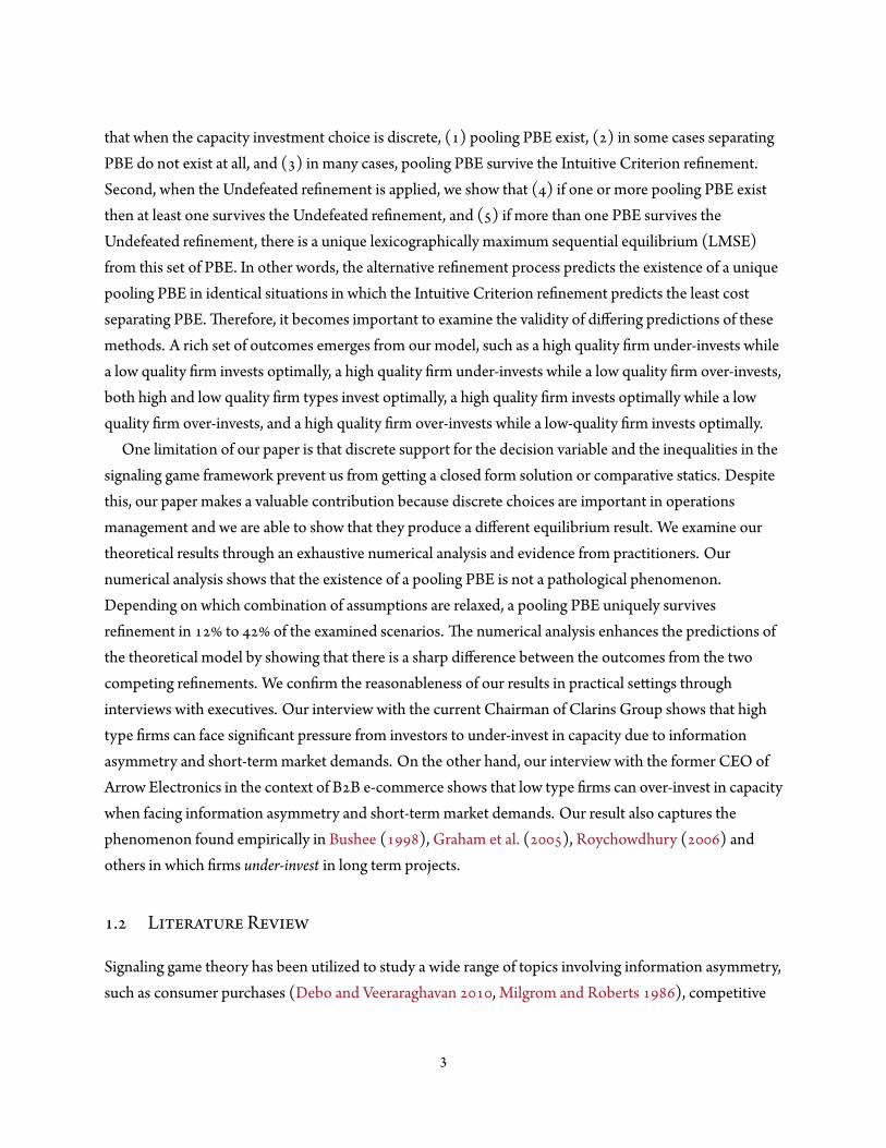
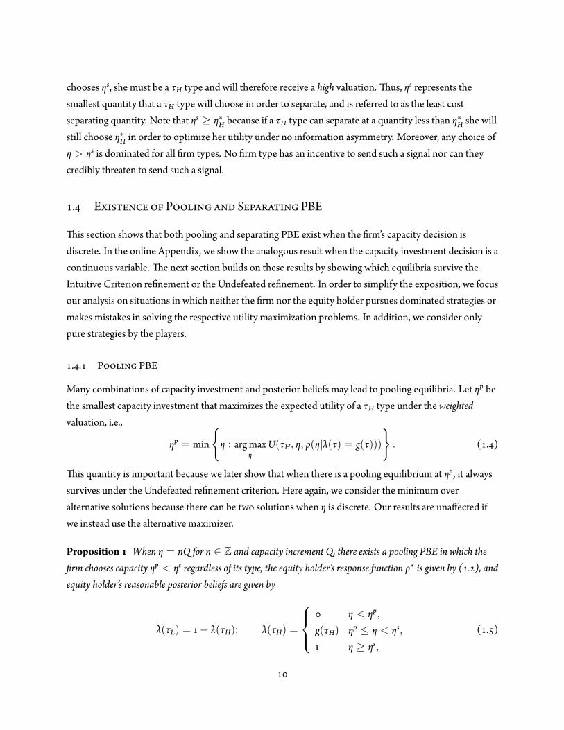
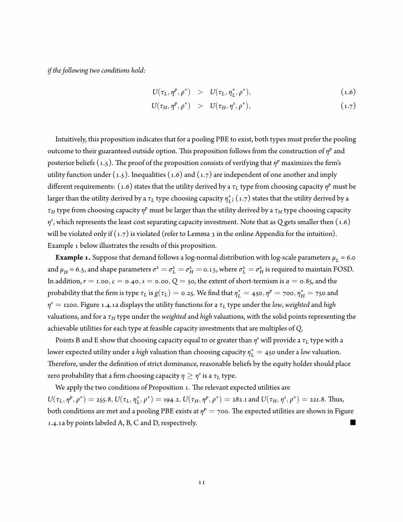
Example . Suppose that demand follows a log-normal distribution with log-scale parameters μL = .and μH = . , and shape parameters σ = σL = σH = . , where σL = σH is required to maintain FOSD.In addition, r = . , c = . , s = . ,Q = , the extent of short-termism is α = . , and theprobability that the rm is type τL is g(τL) = . . We nd that η∗L = , ηp = , η∗H = andηs = . Figure . . a displays the utility functions for a τL type under the low, weighted and highvaluations, and for a τH type under the weighted and high valuations, with the solid points representing theachievable utilities for each type at feasible capacity investments that are multiples ofQ.

Points B and E show that choosing capacity equal to or greater than ηs will provide a τL type with alower expected utility under a high valuation than choosing capacity η∗L = under a low valuation.

erefore, under the de nition of strict dominance, reasonable beliefs by the equity holder should placezero probability that a rm choosing capacity η ≥ ηs is a τL type.

We apply the two conditions of Proposition . e relevant expected utilities areU(τL, ηp, ρ∗) = . ,U(τL, η∗L, ρ

∗) = . ,U(τH, ηp, ρ∗) = . andU(τH, ηs, ρ∗) = . . us,both conditions are met and a pooling PBE exists at ηp = . e expected utilities are shown in Figure. . a by points labeled A, B, C and D, respectively. �

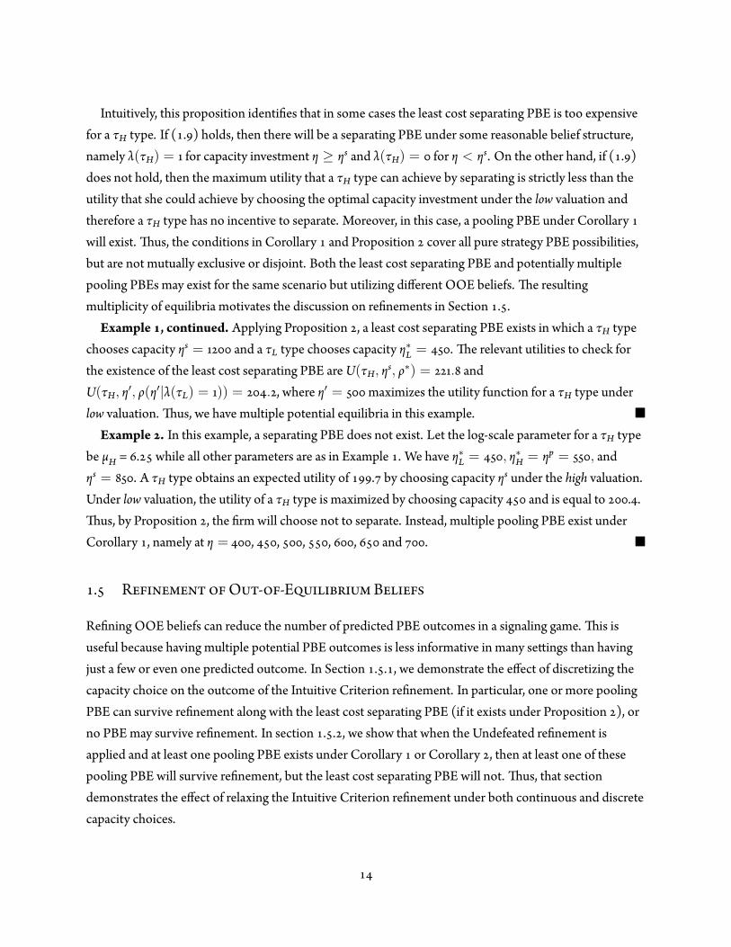
Figure . . : Utility functions for a τL type under the low, weighted and high valuation, and for aτH type under the weighted and high valuation. The model parameters are: α = 0.85, g(τL) =0.25, demand follows a log-normal distribution with log-scale parameters μL = 6.0 and μH = 6.5,shape parameters σ = 0.15, r = 1.00, c = 0.40, s = 0.00, Q = 50.

(a)Firm utility functions showing a poolingPBE at ηp = 700.

(b)Firm utility functions showing that thepooling PBE at ηp = 700 survives the Intu-itive Criterion refinement.

. . M P PBE

Other pooling PBE can be similarly constituted using different reasonable belief structures for the equityholder. Let ηgp be any capacity investment less than ηs. Corollary (proof omi ed) helps us determine allpossible values of ηgp at which there will be a pooling PBE under reasonable beliefs.

Corollary When η = nQ for n ∈ Z and capacity increment Q, there exists a pooling PBE in which the rmchooses capacity ηgp < ηs regardless of its type, the equity holder’s response function ρ∗ is given by ( . ), andposterior beliefs which are reasonable under strict dominance are given by

λ(τL) = − λ(τH); λ(τH) =

η < ηs and η ̸= ηgp,

g(τH) η = ηgp,η ≥ ηs,

( . )

if the following three conditions hold:

U(τL, ηgp, ρ∗) > U(τL, η∗L, ρ∗),

U(τH, ηgp, ρ∗) > U(τH, ηs, ρ∗),

U(τH, ηgp, ρ∗) > maxη′

U(τH, η′, ρ(η′|λ(τL) = )).

Corollary identi es all possible pooling PBE under reasonable beliefs since ( . ) represents theposterior beliefs that are most conducive to a pooling PBE under strict dominance. Other posteriorbeliefs may also support these pooling PBE. e rst two conditions in the corollary are identical to thosein Proposition applied to ηgp instead of ηp. e third condition is new. It states that the utility derived bya τH type at ηgp must exceed the highest possible utility derived by a τH type under low valuation. iscondition is not required in Proposition because it is always met at ηp.

Example , continued. Using Corollary , all of the pooling PBE can be identi ed to be at ηgp = ,, , , , , , , , , and . As noted earlier for this example, ηs = . For

each pooling PBE,U(τL, ηgp, ρ∗) > U(τL, η∗L, ρ∗) = . ,U(τH, ηgp, ρ∗) > U(τH, ηs, ρ∗) = . , and

U(τH, ηgp, ρ∗) > U(τH, η′, ρ(η′|λ(τL) = ) = . , where η′ = maximizes the utility function for aτH type under low valuation. us, all the conditions of Corollary are met. �

We show in the online Appendix that pooling PBE exist if we assume that the capacity investment, η,has continuous support onℜ+. Assuming continuous support allows us to simplify Proposition andCorollary , which we restate in the online Appendix as Proposition and Corollary .

. . S PBE

e least cost separating PBE has a τL type choosing η = η∗L and a τH type choosing ηs, which respectivelyrepresent their optimal capacity investment choices in a separating PBE under reasonable beliefs. Weshow in Proposition that a separating PBE may not exist under discrete capacity choice. is resultcomplements previous papers in the literature, which show that the least cost separating PBE always existsfor continuous capacity investment levels.

Proposition e least cost separating PBE cannot exist under any reasonable belief structure unless:

U(τH, ηs, ρ∗) ≥ maxη′

U(τH, η′, ρ(η′|λ(τL) = )). ( . )

Intuitively, this proposition identi es that in some cases the least cost separating PBE is too expensivefor a τH type. If ( . ) holds, then there will be a separating PBE under some reasonable belief structure,namely λ(τH) = for capacity investment η ≥ ηs and λ(τH) = for η < ηs. On the other hand, if ( . )does not hold, then the maximum utility that a τH type can achieve by separating is strictly less than theutility that she could achieve by choosing the optimal capacity investment under the low valuation andtherefore a τH type has no incentive to separate. Moreover, in this case, a pooling PBE under Corollarywill exist. us, the conditions in Corollary and Proposition cover all pure strategy PBE possibilities,but are not mutually exclusive or disjoint. Both the least cost separating PBE and potentially multiplepooling PBEs may exist for the same scenario but utilizing different OOE beliefs. e resultingmultiplicity of equilibria motivates the discussion on re nements in Section . .

Example , continued. Applying Proposition , a least cost separating PBE exists in which a τH typechooses capacity ηs = and a τL type chooses capacity η∗L = . e relevant utilities to check forthe existence of the least cost separating PBE areU(τH, ηs, ρ∗) = . andU(τH, η′, ρ(η′|λ(τL) = )) = . , where η′ = maximizes the utility function for a τH type underlow valuation. us, we have multiple potential equilibria in this example. �

Example . In this example, a separating PBE does not exist. Let the log-scale parameter for a τH typebe μH = . while all other parameters are as in Example . We have η∗L = , η∗H = ηp = , andηs = . A τH type obtains an expected utility of . by choosing capacity ηs under the high valuation.Under low valuation, the utility of a τH type is maximized by choosing capacity and is equal to . .

us, by Proposition , the rm will choose not to separate. Instead, multiple pooling PBE exist underCorollary , namely at η = , , , , , and . �

. R O - -E B

Re ning OOE beliefs can reduce the number of predicted PBE outcomes in a signaling game. is isuseful because having multiple potential PBE outcomes is less informative in many se ings than havingjust a few or even one predicted outcome. In Section . . , we demonstrate the effect of discretizing thecapacity choice on the outcome of the Intuitive Criterion re nement. In particular, one or more poolingPBE can survive re nement along with the least cost separating PBE (if it exists under Proposition ), orno PBE may survive re nement. In section . . , we show that when the Undefeated re nement isapplied and at least one pooling PBE exists under Corollary or Corollary , then at least one of thesepooling PBE will survive re nement, but the least cost separating PBE will not. us, that sectiondemonstrates the effect of relaxing the Intuitive Criterion re nement under both continuous and discretecapacity choices.

. . T I C R

e Intuitive Criterion re nement is applied by evaluating all possible OOE capacity investment levels fora particular PBE and identifying whether, compared to the PBE results, a capacity investment existswhich would not provide a τL type with a higher utility using a high valuation but would provide a τH typewith a higher utility using a high valuation. If such a capacity investment does exist then the PBE iseliminated. e least cost separating PBE, if it exists under Proposition , survives the Intuitive Criterionre nement by construction. e formal de nition of the Intuitive Criterion re nement is developed inCho and Kreps ( ) and provided in the Appendix using our notation. e following proposition givesthe conditions for the pooling PBE at ηp to survive the Intuitive Criterion.

Proposition e pooling PBE identi ed in Proposition will survive the Intuitive Criterion re nement if andonly if there does not exist a capacity investment, η′, for which both of the following conditions are true: (i)U(τL, ηp, ρ∗) > U(τL, η′, ρ(η′|λ(τH) = )) and (ii) U(τH, ηp, ρ∗) < U(τH, η′, ρ(η′|λ(τH) = )).

In words, the rst condition states that the utility for a τL type is greater at the pooling PBE involving ηp

than at an alternative capacity investment, η′, under a high valuation. e second condition states that theutility for a τH type is less at the pooling PBE involving ηp than at this alternative capacity investment, η′,under a high valuation. If an alternative capacity investment, η′, that meets both conditions does not existthen the equilibrium will survive the Intuitive Criterion re nement. By replacing ηp with ηgp, Propositioncan equivalently be used to test whether any of the pooling PBE identi ed by Corollary also survives

the Intuitive Criterion re nement.Note that the conditions in Proposition are always satis ed (i.e., an η′ will always exist) for capacity

decisions with continuous support. erefore, no pooling PBE will survive the Intuitive Criterionre nement if the decision space is continuous in a game such as ours, i.e. a game with two types of theinformed player and a single costly signal with in nite support (Cho and Kreps , Mas-Colell et al.

). In contrast, Proposition implies that multiple equilibria can survive the Intuitive Criterionre nement, including the least cost separating equilibrium and one or more pooling PBE, if the decisionspace is discrete. us, this re nement does not result in a unique prediction under discrete capacitychoice.

We consider alternatives to this re nement method because the Intuitive Criterion may not beappropriate in all operations management se ings. As noted by Bolton and Dewatripont ( ), “asplausible as the Cho-Kreps Intuitive Criterion may be, it does seem to predict implausible outcomes insome situations.” Indeed, the application of certain belief-based re nements such as the Intuitive Criterionis unse led in the game theory literature (Mailath et al. , Riley ). One concern is that a τH typeis presumed to choose the separating capacity investment, ηs, even if such a choice is Pareto-dominated bya pooling capacity investment. e Intuitive Criterion re nement does not eliminate the separating

equilibrium even if the probability of the rm being a τL type approaches zero (Bolton and Dewatripont, Kreps and Sobel ). is results in a discontinuity in the choice of capacity investment for a τH

type (from ηs to η∗H) when g(τL) goes from a value of ε > to (Mailath et al. ).A second concern is that the Intuitive Criterion assumes that the participants in the game can

communicate counterfactual information to other participants by way of “speeches,” but these speechesare not explicitly modeled in the game (Salanie ). One implication of this is that the equity holder’sbeliefs, speci cally their beliefs at the proposed OOE point, are not fully updated by the application of theIntuitive Criterion. is casts doubt on whether the deviation proposed by the Intuitive Criterion canactually be considered an unambiguous signal of the rm’s type (Mailath et al. ).

A third concern is that when a least cost separating PBE does not exist (as in Proposition ) then theIntuitive Criterion re nement may actually eliminate all PBE in the game. is eliminates any predictivepower that would otherwise be provided from the analysis of the signaling game. Example , summarizedin Table . . , shows such an outcome.

Example , continued. is example shows that multiple PBE survive the Intuitive Criterionre nement. e least cost separating PBE in which a τH type chooses capacity ηs = and a τL typechooses capacity η∗L = survives the Intuitive Criterion re nement by construction. Based onProposition , the pooling PBEs at , , and also survive the Intuitive Criterion re nement.Figure . . b shows this in greater detail for the pooling PBE at ηp = . Compared to the pooling PBEat ηp = , a τL type is willing to invest in capacity up to units in order to receive a high valuation,but a τH type is unwilling to invest in capacity more than units in order to receive a high valuation inlieu of the weighted valuation. erefore, as required by Proposition , there is no capacity investment towhich a τH type is willing to deviate from ηp under a high valuation but a τL type is unwilling to deviatefrom ηp under a high valuation.

Example . is example illustrates the rst criticism of the Intuitive Criterion re nement, namelythat it may identify the least cost separating PBE as the unique surviving PBE even if another PBE is aPareto improvement over it. Let demand follow a log-normal distribution with log-scale parameter μL =. , μH = . and shape parameters σ = . , and the remaining model parameters be r = . , c = . , s

= . , α = . , g(τL) = . , andQ = . ere are several pooling PBE, including one at ηp = , ,which results in expected utilities of . for a τH type, . for a τL type, and for the equity holder.However, this pooling PBE is eliminated by the application of the Intuitive Criterion re nement. In fact,the only equilibrium that survives the Intuitive Criterion re nement is the least cost separating PBE inwhich a τH type chooses capacity ηs = , and a τL type chooses capacity η∗L = . is separatingPBE results in a utility of . for a τH type (a decrease of . compared to the pooling PBE at ηp), autility of . for a τL type (a decrease of . compared to the pooling PBE at ηp) and a utility of for

the equity holder (so the equity holder is indifferent between the two equilibria). �

. . T U R

In light of the concerns raised about the Intuitive Criterion re nement, an alternative re nement processmay be warranted in some circumstances. e Undefeated re nement is applied by iterating across allpossible PBE in the model and identifying whether the beliefs used to support each PBE are reasonablegiven the other possible PBE and the preferences for each rm type among those PBE. PBE that rely onbeliefs that are unreasonable in this regard are eliminated. e formal de nition of the Undefeatedre nement is developed in Mailath et al. ( ) and summarized in the Appendix using our notation.

e Undefeated re nement has been applied in the nance and economics literature (Fishman andHagerty , Gomes , Spiegel and Spulber , Taylor ) and it addresses many of theconcerns raised about the Intuitive Criterion re nement. By construction the Undefeated re nementdoes not eliminate any PBE that is Pareto efficient, as is possible with the Intuitive Criterion re nement.In addition, unlike the Intuitive Criterion re nement, the Undefeated re nement does not rely onunmodeled “speeches” from the rm in order to convey additional information to the equity holder.Instead, the Undefeated re nement ensures that OOE beliefs are restricted only by other equilibria in themodel. Finally, at least one PBE will survive the Undefeated re nement since it eliminates PBE byperforming a Pareto comparison to other PBE.

Proposition If one or more pooling PBE exists under reasonable beliefs as in Corollary or Corollary , then(i) at least one of those PBE will survive the Undefeated re nement, and (ii) the least cost separating PBE, if itexists, will not survive the Undefeated re nement.

e intuition behind Proposition is that at least one of the pooling PBE identi ed using Corollariesor will not be Pareto dominated by any other PBE. If the least cost separating equilibrium also existsunder Proposition then every pooling PBE that exists is by de nition a Pareto improvement over theseparating PBE. A corollary result to Proposition is that the least cost separating PBE is the uniqueUndefeated PBE if and only if a pooling PBE does not exist under reasonable beliefs. Examples - ,summarized in Table . . , illustrate these possibilities.

If multiple pooling PBE survive the Undefeated re nement, we apply the concept of lexicographicallymaximum sequential equilibrium (LMSE) to identify a unique PBE. According to Mailath et al. ( ), aPBE is a LMSE if among all PBE it maximizes the utility for a τH type and conditional on maximizing theutility for a τH type, it then maximizes the utility for a τL type. Using a LMSE to identify a unique PBE isintuitively appealing because typically a low-quality rm wishes to masquerade as a high-quality rmrather than the opposite, so resolving on a belief structure that supports such an outcome seemsreasonable (Taylor ). e alternative would be to use a belief structure that increases the utility of a

τL type but decreases the utility of a τH type compared to the utilities achieved at the LMSE, which ismore difficult to justify.

Due to the concavity of the utility functions, a unique LMSE will always exist among the PBE thatsurvive the Undefeated re nement. If one of the pooling PBEs is at ηp, then this will be the unique PBEwhich is a LMSE since it maximizes the utility of a τH type and conditional on that, maximizes the utilityof a τL type.

Example , continued. Of all the possible pooling and separating PBE, the pooling PBEs at η =and survive the Undefeated re nement but the least cost separating PBE does not, in accordance withProposition . e pooling PBE at η = yields a utility of . for a τL type and . for a τH type.Both rms receive a greater utility under this pooling PBE than under the pooling PBE at η = , ,

, , , , , , and or under the separating PBE. erefore, each of these PBE aredefeated by the pooling PBE at η = . Similarly, the pooling PBE at η = yields a utility of . fora τL type and . for a τH type, and defeats the pooling PBE at η = , , , , , , ,

and as well as the separating PBE. No other PBE defeats the pooling PBE at η = or . epooling PBE at η = provides the maximum utility for a τH type and is therefore the unique PBEwhich is a LMSE. �

Table . . summarizes the results of Examples - and presents two additional examples illustratingvarious results of our paper. In Example , the least cost separating PBE and many pooling poolingequilibria survive the Intuitive Criterion re nement, and the pooling equilibrium at ηp is the uniqueLMSE prediction. In Example , a separating PBE does not exist, but multiple pooling PBE exist underCorollary . e pooling PBE at η = , , and survive the Intuitive Criterion re nement.

e pooling PBE at η = is the only PBE to survive the Undefeated re nement and it is a LMSE.Example , shown in Section . . , highlights the rst criticism of the Intuitive Criterion re nement:although the pooling PBE at ηp is a Pareto improvement over the least cost separating PBE, the IntuitiveCriterion implies that both types will instead choose the least cost separating equilibrium. eUndefeated re nement, on the other hand, eliminates the least cost separating PBE in favor of the poolingPBE at ηp.

Example illustrates the signi cance of Corollary by showing that pooling at lowmay occur anduniquely survive re nement, i.e., a τH type may choose the capacity level η∗L which maximizes the utilityof a τL type under low valuation. ere is no pooling PBE at ηp = units because ( . ) in Propositionis violated (the utility of a τL type at ηp is . and at η∗L is . ), so a τL type would prefer to separatethan to choose capacity ηp. ere is no separating PBE either, because Inequality ( . ) in Proposition isviolated (ηs = and results in a utility of . for a τH type while her maximum utility under the lowvaluation is . ), so a τH type is unwilling to separate. Under Corollary , however, there is a pooling

Table . . : Examples illustrating the PBE that exist and survive refinement. In each example, μL= 6.00, c = 0.40, and the other parameters are as listed. The first row in each example givesresults for pooling PBE and the second row gives results for separating PBE. For instance, inExample 1, there are several pooling PBE at ηgp = 400, 450, …, 950 and there is a separatingPBE in which a τL type chooses η = 450 and a τH type chooses η = 1200. The latter survivesthe Intuitive Criterion but does not survive the Undefeated refinement.

Ex. Model Parameters PBE Capacities PBE Capacities Surviving Re nementμH σ r s Q α g(τL) Intuitive Undefeated LMSE

. . . . . . ≤ ηgp ≤ , , , ,τL : , τH : Yes No No

. . . . . . ≤ ηgp ≤ , , ,None - - -

. . . . . . ≤ ηgp ≤ See Note ≤ ηgp ≤τL : , τH : Yes No No

. . . . . . NoneNone - - -

. . . . . . NoneNone - - -

Note: In Ex. , pooling PBE survive the Intuitive Criterion. e surviving PBE are sca ered between , and , .

PBE at η = (the utility of a τH type is . and of a τL type is . ). In fact, this is the unique PBEand survives the Intuitive Criterion and Undefeated re nements and it is the unique LMSE. It isinteresting to note that a capacity investment at η = maximizes the utility of a τL type under aweighted valuation, but it does not maximize the utility of a τH type under a weighted valuation. It alsomaximizes the utility of a τL type if there were no information asymmetry (i.e. under a low valuation).

is counterintuitive result indicates that there are situations in which a τH type can bene t by adoptingthe preferred capacity investment of a τL type.

In Example , we highlight the third criticism of the Intuitive Criterion re nement mentioned inSection . . , namely that it may result in no PBE solution. ere is no pooling PBE at ηp = unitsbecause ( . ) in Proposition is violated (the utility of a τL type at ηp is . and at η∗L is . ), so a τLtype would prefer to separate than to choose capacity ηp. ere is no separating PBE either, because ( . )in Proposition is violated (ηs = and results in a utility of . for a τH type while her maximumutility under the low valuation is . ), so a τH type is unwilling to separate. Under Corollary , however,there is a pooling PBE at η = (the utility of a τH type is . and of a τL type is . ). In fact, thisPBE survives the Undefeated re nements and is the unique LMSE. It does not, however, survive theIntuitive Criterion.

. N A

We conduct a numerical analysis to assess the likelihood of pooling PBE occurring and survivingre nement, and to determine the effect of the model parameters on this likelihood. We use the following

setup. e rm faces a log-normal demand distribution regardless of its type. e log-scale parameter fora τL type is μL = . , and for a τH type is μH ∈ { . , . , . }. e shape parameter takes valuesσ ∈ { . , . , . }. e unit price (r) ranges from . to . in increments of . , unit salvage value(s) ranges from . to . in increments of . , and unit cost is xed at c = . . Short-termism (α)ranges from . to . in increments of . , the equity holder’s prior beliefs that the rm is type τL(g(τL)) ranges from . to . in increments of . , and the capacity investment is either continuousor discrete withQ ∈ { , , }. We run , , scenarios with these parameters. In these scenarios,we use Proposition instead of Corollary to check for the existence of pooling PBE, and thus restrictourselves only to pooling PBE at η = ηp. is simpli es the analysis and makes it a conservativeassessment of the likelihood of a pooling PBE because additional pooling PBE may exist under Corollary.We are particularly interested in demonstrating the impact of the newsvendor model parameters on the

existence of a pooling PBE. In the newsvendor model, increasing either the cost of underage or the cost ofoverage vertically translates the expected pro t function with the amount of the translation increasing ascapacity increases (refer to Lemma ). is increases the utility from the various utility functions at eachcapacity level, and increases the skewness of the utility functions. e Undefeated re nement relies uponPareto optimization across alternatives, making it sensitive to increases in utility. e Intuitive Criterionre nement utilizes non-equilibrium preferences that are sensitive to the skewness of the utility functions.

is implies that the impact of increasing price or salvage value on the likelihood of a pooling PBE willdiffer depending on whether the Undefeated or the Intuitive Criterion re nement is asserted. We seek toclearly reveal this behavior in our numerical analysis.

Since we have a large number of parameters and many scenarios, we apply regression analysis to assessthe effects of newsvendor parameters on the occurrence of pooling equilibria. While these regressionresults cannot be generalized beyond the numerical analysis, it allows us to efficiently examine andcompare all of the combinations of the assumption relaxations that we have proposed. We separate theanalysis into three situations: continuous support with the Undefeated re nement, discrete support withthe Intuitive Criterion re nement, and discrete support with the Undefeated re nement. A logit model isused with a binary dependent variable, Pooling PBE, which is equal to when a pooling PBE at ηp existsand survives re nement, and otherwise. e explanatory variables consist of the price (Price), thesalvage value (Salvage), the scale parameter of a τH type (ScaleHigh), the shape parameter (Shape), theprior beliefs of the equity holder (PriorLow), short-termism (ShortTermism), and the capacity increment(CapacityIncrement). Since the regression model is an approximation, we employ quadratic andinteraction terms for price and salvage value to model non-linearity. ese variables are mean-centered toaid in the interpretation of the quadratic and interaction terms, but mean-centering does not affect the

marginal impact of the variables in the model. Our primary speci cation is:

Pooling PBEi =α + β · Pricei + β · Salvagei + β · Pricei + β · Salvagei+

β · Pricei × Salvagei + β · ScaleHighi + β · Shapei+

β · PriorLowi + β · ShortTermismi + β · CapacityIncrementi + εi,

( . )

where i identi es the scenario from the numerical analysis. We evaluate alternative speci cations and theprimary inferences are similar. Due to space constraints, we present estimates for a subset of thosespeci cations.

Table . . shows the results of the logit regressions. Columns and present estimation results forcontinuous support and the Undefeated re nement, which is addressed by , scenarios in thenumerical analysis, Columns and present results for discrete support and the Intuitive Criterionre nement ( , scenarios), and Columns and for discrete support and the Undefeatedre nement ( , scenarios). Columns , and exclude the square and interaction terms whileColumns , and include those terms. Likelihood ratio tests indicate that the models in Columns ,and provide a be er t than Columns , and , respectively. We discuss the results in Column , and, which subsume the inferences from column , , and .

e main inferences from this analysis are as follows. We observe that the existence of a pooling PBE isnot a pathological phenomenon. Across the , scenarios which use continuous support and theUndefeated re nement, a pooling PBE exists and survives re nement of the time. is percentage is

for the , scenarios which use discrete support and the Intuitive Criterion, and for the, scenarios which use discrete support and the Undefeated re nement. e pseudo R-square of

the logit model is higher than under Undefeated re nement and higher than under IntuitiveCriterion re nement. e newsvendor parameters have contrasting effects on the probability ofoccurrence of a pooling PBE under Undefeated and Intuitive Criterion re nements. Speci cally, thelikelihood of a pooling equilibrium increases in price and salvage value under Undefeated re nement anddecreases in price and salvage value under Intuitive Criterion re nement. is contrast is valuablebecause it can be used empirically to test which re nement is more representative of real data. Similar toprice and salvage value, σ has different effects on the likelihood of pooling equilibria under theUndefeated and Intuitive Criterion re nements. With respect to the remaining parameters, theprobability of a pooling equilibrium increases in short-termism α, decreases in the prior probability of arm being low type g(τL), increases in μH, and increases in the capacity incrementQ.We discuss some of the effects in detail. Changing price is equivalent to changing the cost of underage

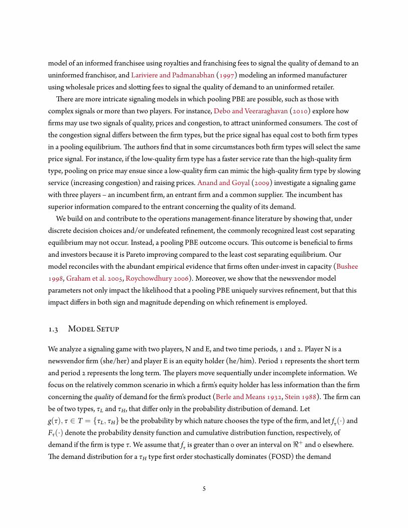
r− c. Figure . . a displays the average marginal effect of Price over the examined range of values ofSalvage. We construct this gure because the marginal effect of Price depends on linear, quadratic and

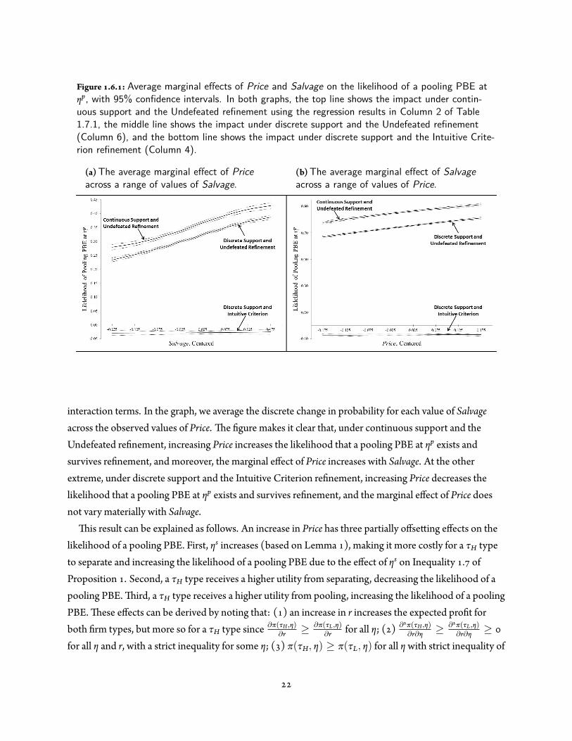
Figure . . : Average marginal effects of Price and Salvage on the likelihood of a pooling PBE atηp, with 95% confidence intervals. In both graphs, the top line shows the impact under contin-uous support and the Undefeated refinement using the regression results in Column 2 of Table1.7.1, the middle line shows the impact under discrete support and the Undefeated refinement(Column 6), and the bottom line shows the impact under discrete support and the Intuitive Crite-rion refinement (Column 4).

(a)The average marginal effect of Priceacross a range of values of Salvage.

(b)The average marginal effect of Salvageacross a range of values of Price.

interaction terms. In the graph, we average the discrete change in probability for each value of Salvageacross the observed values of Price. e gure makes it clear that, under continuous support and theUndefeated re nement, increasing Price increases the likelihood that a pooling PBE at ηp exists andsurvives re nement, and moreover, the marginal effect of Price increases with Salvage. At the otherextreme, under discrete support and the Intuitive Criterion re nement, increasing Price decreases thelikelihood that a pooling PBE at ηp exists and survives re nement, and the marginal effect of Price doesnot vary materially with Salvage.

is result can be explained as follows. An increase in Price has three partially offse ing effects on thelikelihood of a pooling PBE. First, ηs increases (based on Lemma ), making it more costly for a τH typeto separate and increasing the likelihood of a pooling PBE due to the effect of ηs on Inequality . ofProposition . Second, a τH type receives a higher utility from separating, decreasing the likelihood of apooling PBE. ird, a τH type receives a higher utility from pooling, increasing the likelihood of a poolingPBE. ese effects can be derived by noting that: ( ) an increase in r increases the expected pro t forboth rm types, but more so for a τH type since ∂π(τH,η)

∂r ≥ ∂π(τL,η)∂r for all η; ( ) ∂ π(τH,η)

∂r∂η ≥ ∂ π(τL,η)∂r∂η ≥

for all η and r, with a strict inequality for some η; ( ) π(τH, η) ≥ π(τL, η) for all η with strict inequality of

some η (for ( ), ( ) and ( ), refer to Lemma ); and ( ) the utility functions for both rm types aresimply linear combinations of the expected pro t functions for each rm type (refer to Equation . ).Increasing Price in the newsvendor model vertically translates the expected pro t function, with theamount of the translation increasing in the capacity investment, η (refer to Lemma ). As a result, the rstand third effects dominate, resulting in a net increase in the likelihood of a pooling PBE.

Price has a different effect when the Intuitive Criterion re nement is applied, however. e IntuitiveCriterion re nement speci es a capacity investment range which will re ne away a pooling PBE if there isa capacity investment alternative within this range. e low end of this range is de ned by the continuousvalue of capacity which just satis es ( ). is represents the value above which a τL type is unwilling todeviate from the pooling equilibrium even if it were to result in a high valuation. e high end of this rangeis that which just satis es ( . ). is represents the value above which a τH type is unwilling to deviatefrom the pooling equilibrium even if it were to result in a high valuation. Since increasing Price in thenewsvendor model increases the skew of the utility functions, the capacity investment range speci ed bythe Intuitive Criterion increases and it is less likely that the pooling PBE will survive re nement. iseffect can be derived by noting that: ( ) ∂ π(τH,η)

∂r∂η ≥ ∂ π(τL,η)∂r∂η ≥ for all η and r, with a strict inequality for

some η (refer to Lemma ) and ( ) the utility functions for both rm types are simply linearcombinations of the expected pro t functions for each rm type (refer to Equation . ).

Figure . . illustrates this effect by depicting the capacity range over which pooling equilibria areeliminated by the Intuitive Criterion re nement. We expand the set of values for Price to make the effectmore apparent. As Price increases, the range increases in a saw-toothed pa ern, and it becomes morelikely to nd a discrete capacity nQ in this range which will eliminate pooling PBE.

e impact of a change in salvage value is equivalent to a change in the cost of overage, c− s. Figure. . b uses the results in Columns , , and of Table . . to show that there is a signi cant difference in

the average marginal effect of Salvage over the examined range of values of Price. Under continuoussupport and the Undefeated re nement, increasing Salvage increases the likelihood that a pooling PBE atηp exists and survives re nement, and the marginal effect of Salvage increases with Price. At the otherextreme, under discrete support and the Intuitive Criterion re nement, increasing Salvage decreases thelikelihood that a pooling PBE at ηp exists and survives re nement, and the marginal effect of Salvage doesnot vary materially with Price. e intuition explaining the impact of Salvage is similar to the intuitionexplaining the impact of Price.

We brie y describe the empirical results associated with other parameters in the model. e coefficienton ShortTermism is positive and signi cant regardless of the support and re nement assumptionsemployed. As α increases, the utility received by a τH type in a pooling equilibrium decreases (refer toEquation ( . )). us, pooling becomes less a ractive to a τH type, and she is more willing to over-invest

Figure . . : The capacity investment range in which the Intuitive Criterion refinement will elim-inate a pooling PBE at ηp. Demand follows a log-normal distribution with log-scale parame-ters μL = 6.0 and μH = 6.25, and shape parameters σ = 0.15. In addition, c = . , s =. ,Q = , short-termism α = . , the probability that the firm is type τL is g(τL) = . ,

and r ∈ { . , . , . . . , . }.

to separate. However, a τL type is also more willing to over-invest to garner a higher short-term valuation.is increases the value of ηs such that a pooling outcome becomes more a ractive to a τH type. As α gets

increasingly large, the second effect dominates, resulting in a pooling PBE.e coefficient on PriorLow is negative and signi cant regardless of the support and re nement

assumptions employed. As PriorLow decreases, the short-term valuation that a τH type receives at ηp

increases (refer to Lemma ) and approaches the short-term valuation for a τH type under no informationasymmetry. Simultaneously, ηp approaches η∗H, which increases the expected long-term pro t of a τH typechoosing capacity investment ηp. Both factors make it more a ractive for a τH type to pool than toseparate.

e coefficient on ScaleHigh is also negative and signi cant regardless of the support and re nementassumptions. Intuitively, a lower value of ScaleHighmeans there is less difference in performanceprospects between the two types, which makes a pooling PBE more likely. e coefficient on Shape ispositive and signi cant under continuous support and the Undefeated re nement but negative andsigni cant under discrete support and the Intuitive re nement. e former result occurs because anincrease in Shape increases the skewness of the utility functions, which improves the likelihood of poolingby increasing the cost of separation for a τH type. e la er result is because this increase in the skewnessincreases the likelihood that a discrete capacity investment alternative falls within the capacity rangede ned by the Intuitive Criterion.

e coefficient of CapacityIncrement is consistently positive and signi cant. e utility a τL type isweakly lower at η∗L asQ increases, providing a stronger incentive for a τL type to pool. In addition, thevalue of ηs will be weakly larger asQ increases, which provides a stronger incentive for a τH type to pool.Finally, asQ increases, it is less likely that there will be a capacity investment choice that satis es theconditions of the Intuitive Criterion re nement.

. M I D

. . F S E

Clarins Group. e investment phenomena captured by our model are present in a variety of real-worldsituations. French upscale beauty brand Clarins Group provides an example of how τH types can becompelled to under-invest in capacity. In with a global recession looming, many market analystswere generally pessimistic about sales of high-end beauty products that would be discretionary for manyconsumers and noted that “luring women to invest in high-end skin-care regimens is challenging whenshoppers are cu ing back” (Byron ). Clarins management, however, saw considerable opportunityto sell its products by opening a line of in-store spas, thereby dramatically increasing its retail capacity. In apersonal interview in July , Chairman Christian Courtin-Clarins that as a public company, the rm“felt pressure to make decisions based on quarterly drivers.” Rather than compromise their investmentstrategy, the founding family opted to take the rm private in the summer of . Mr. Courtin-Clarinsrevealed that one in uencing factor was a desire to “have a long-term view in their investment decisions.”By going private, the rm was able to invest substantially in opening “Clarins department-store skin spas”in . Mr. Courtin-Clarins went on to say that it was “absolutely the case” that the spa initiativerequired a large, lumpy investment and that Clarins “could not have made this investment had weremained public.” In the framework of our model, Clarins is a τH type and would have under-invested incapacity had they remained publicly traded. Going private reduced the rm’s emphasis on short-termvaluation (reducing α) and mitigated information asymmetry with its equity holders by moving frompublic market equity holders to private and family equity holders.

A E . Arrow Electronics, a Fortune distributor of electronic components, re ectsa situation in which a τL type over-invests in capacity. In , at the height of the Internet bubble, themarket was richly rewarding Internet initiatives of all forms (captured in our model by a low g(τL)), andmanagers at Arrow Electronics felt tremendous pressure to capitalize on this trend (captured by a high α).Despite the Internet boom, Chairman and CEO Steve Kaufman, with his in-depth knowledge of theindustry, resisted transforming Arrow’s business model. In a personal interview on August , ,

Kaufman contended that the Internet was no panacea and that “while it may help around the edges, theInternet could never replace Arrow’s business model. e enthusiasm of the market, however, inducedpeople to not distinguish between business models that might work and those that wouldn’t.” Feelingcontinued pressure, Arrow eventually made several investments (totaling approximately M) in veInternet ventures, including ChipCenter LLC, QuestLink Technology, and Virtual Chip Exchange.Kaufman noted “You hear the same thing from enough people and it starts to sound real. e Boardbegan worrying about duciary responsibilities and the implications for the rm if I was wrong.”Remarking on the size of the investments, Kaufman noted that “Although the public investors didn’t thinkit was enough, the Board felt it was a good compromise between the outside view and my position thatthe Internet would not jeopardize the company.” He also noted that two factors made their investmentchoice discrete – “ ere was a minimum efficient scale for the investments and for accounting purposeswe wanted to be close to but not exceed a ownership stake in any venture.”

. . D

We investigate the effect on a rm’s capacity decision of short-termism and asymmetric informationbetween the rm and its equity holders. In particular, we explore how the parameters of the newsvendormodel impact the likelihood of a pooling PBE a er relaxing common modeling assumptions so we maybe er account for real-world and operations-relevant constraints, such as discrete investment levels andPareto-optimization decision rules. While stylized models in economics o en employ these assumptions,operations management o en deals with real-world aspects of decision problems. We strengthen thecurrent operations management literature by not only showing that these real-world considerations leadto different outcomes than shown by the stylized economic models, but that the newsvendor modelparameters play an important and counter-intuitive role in these outcomes. We are able to explain abroader set of outcomes than prior research (Bebchuk and Stole , Lai et al. ), and reconcile thisliterature with empirical studies which have found that rms under-invest in long term projects (Bushee

, Graham et al. , Roychowdhury ).Our analysis provides evidence that rms have incentives to establish or maintain discrete capacity

commitments. We show that in many circumstances the rm receives a higher utility from a pooling PBEcompared to the least cost separating PBE, regardless of the rm’s type. If the rm otherwise operates inan environment in which the capacity investment level has continuous support and beliefs are re nedusing logic similar to the Intuitive Criterion, then the rm can avoid costly separating by making acredible a priori commitment to adhere to discrete capacity investments. Firms can achieve this, forinstance, by signing capacity contracts that have onerous terms if capacity is not ordered in discreteincrements. Since the pooling PBE outcome is bene cial to both types of rms, the rm has incentives to

make such credible commitments early, and even prior to the rm realizing its type.Our paper can be extended and modi ed in subsequent research in other ways. For instance, future

empirical work may exploit the nding that relaxing different modeling assumptions leads the parametersof the newsvendor model to have a different impact on the likelihood of a pooling PBE. Doing so willallow researchers to identify which assumptions more accurately re ect reality in different operatingenvironments. In addition, our model can be employed to evaluate the impact of other types ofinformation asymmetry, including information asymmetry on the rm’s operating costs or its exposure todisruption risk. Finally, additional research can consider the impact of relaxing other modelingassumptions, including assumptions that there is in nite signal support and only two types of theinformed player. Relaxing either assumption may also result in a pooling PBE uniquely survivingre nement. e intuition for the former is that when the signal is physically constrained to be less than ηs

then it is impossible for a τH type to separate. e intuition for the la er is more involved, but welldescribed in Cho and Kreps ( ). It is not immediately clear, however, what the implications of suchrelaxations are on the impacts of the newsvendor model parameters on the resulting PBE. We leave this tofuture research.

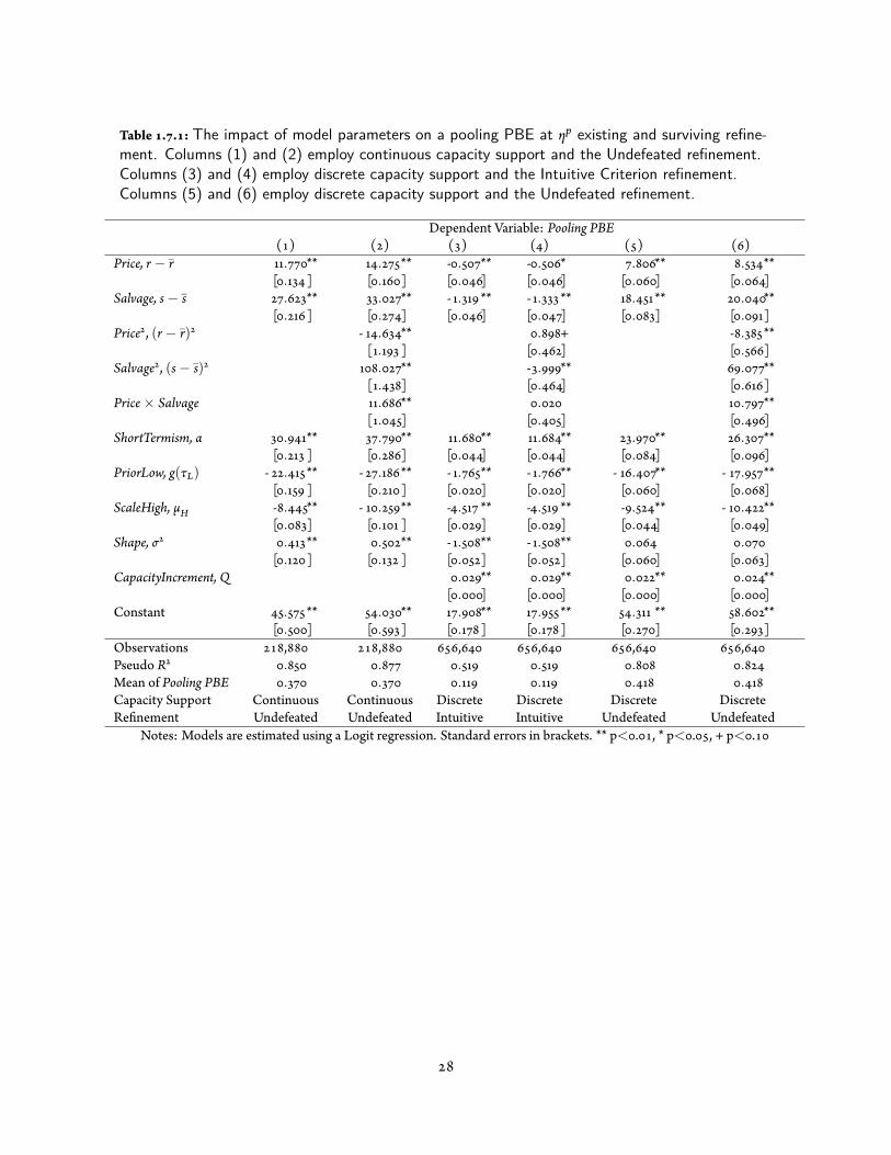
Table . . : The impact of model parameters on a pooling PBE at ηp existing and surviving refine-ment. Columns (1) and (2) employ continuous capacity support and the Undefeated refinement.Columns (3) and (4) employ discrete capacity support and the Intuitive Criterion refinement.Columns (5) and (6) employ discrete capacity support and the Undefeated refinement.

Dependent Variable: Pooling PBE( ) ( ) ( ) ( ) ( ) ( )

Price, r− r̄ . ** . ** - . ** - . * . ** . **[ . ] [ . ] [ . ] [ . ] [ . ] [ . ]

Salvage, s− s̄ . ** . ** - . ** - . ** . ** . **[ . ] [ . ] [ . ] [ . ] [ . ] [ . ]

Price , (r− r̄) - . ** . + - . **[ . ] [ . ] [ . ]

Salvage , (s− s̄) . ** - . ** . **[ . ] [ . ] [ . ]

Price× Salvage . ** . . **[ . ] [ . ] [ . ]

ShortTermism, α . ** . ** . ** . ** . ** . **[ . ] [ . ] [ . ] [ . ] [ . ] [ . ]

PriorLow, g(τL) - . ** - . ** - . ** - . ** - . ** - . **[ . ] [ . ] [ . ] [ . ] [ . ] [ . ]

ScaleHigh, μH - . ** - . ** - . ** - . ** - . ** - . **[ . ] [ . ] [ . ] [ . ] [ . ] [ . ]

Shape, σ . ** . ** - . ** - . ** . .[ . ] [ . ] [ . ] [ . ] [ . ] [ . ]

CapacityIncrement, Q . ** . ** . ** . **[ . ] [ . ] [ . ] [ . ]

Constant . ** . ** . ** . ** . ** . **[ . ] [ . ] [ . ] [ . ] [ . ] [ . ]

Observations , , , , , ,Pseudo R . . . . . .Mean of Pooling PBE . . . . . .Capacity Support Continuous Continuous Discrete Discrete Discrete DiscreteRe nement Undefeated Undefeated Intuitive Intuitive Undefeated Undefeated

Notes: Models are estimated using a Logit regression. Standard errors in brackets. ** p< . , * p< . , + p< .

A –D

e following de nitions are restated in our notation and re ect our focus on pure strategies.

De nition Perfect Bayesian Equilibrium. According to Fudenberg and Tirole ( ), a PBE of a

signaling game consists of a strategy pro le, φ∗, and posterior beliefs, λ(τ). In the context of pure

strategies, a strategy pro le for the rm (player N), φN(τ), is a capacity investment, η, for each rm type,

τ. A strategy pro le for the equity holder (player E), φE(η), is an equity price, ρ(η), assigned to the rm

for each capacity investment of the rm, η. e strategy pro les must be such that for the rm,

φ∗N(τ) = argmaxη U(τ, η, ρ), for all τ. For the equity holder, φ∗E(η) = argmaxρ∑

τ λ(τ)V(τ, η, ρ), for all

η.

In addition, if∑

τ′∈T g(τ′) [φ∗N(τ

′) = η] > so that Bayes rule can be applied, then the equity holder’s

posterior beliefs are λ(τ) = g(τ) [φ∗N(τ)=η]∑τ′∈T g(τ′) [φ∗N(τ′)=η] , where g(τ) is the equity holder’s prior beliefs. If∑

τ′∈T g(τ′) [φ∗N(τ

′) = η] = , then Bayes rule cannot be applied and the equity holder’s posterior

beliefs, λ(τ), may be any probability distribution on T. �De nition Strict Dominance. Mas-Colell et al. ( , p. ) state that a signal, η, is strictly

dominated for a type τ i ∈ T if there exists another signal η′ such that the following inequality holds:

maxρ∈P∗(T,η)

U(τ i, η, ρ) < minρ∈P∗(T,η′)

U(τ i, η′, ρ). ( . )

Form the set S(η) consisting of all types τ i such that this inequality does not hold. en a PBE has

reasonable beliefs if for all η with S(η) ̸= ∅, λ(τ i) > only if τ i ∈ S(η). �In words, ( . ) states that a signal is strictly dominated for a type if the best utility which that type

could possibly achieve by sending that signal is strictly lower than the worst utility which that type could

possibly achieve by sending some other signal. A PBE has reasonable beliefs if those beliefs do not put a

positive probability on any type sending a signal that is strictly dominated.

De nition Intuitive Criterion Re nement. According to Cho and Kreps ( ), the Intuitive

Criterion re nement is applied in two steps to evaluate a PBE involving η and ρ∗:

. Form the set S(η′) for all η′ ̸= η consisting of all types τ such that

U(τ, η, ρ∗) > maxρ∈P∗(T,η′)

U(τ, η′, ρ). ( . )

. If, for some out of equilibrium signal η′, there exists some type τ′ ∈ T\S(η′) such that

U(τ′, η, ρ∗) < minρ∈P∗(T\S(η′),η′)

U(τ′, η′, ρ), ( . )

then the equilibrium fails the Intuitive Criterion. �

In words, S(η′) consists of all types whose expected utility from choosing the in-equilibrium capacity

investment, η, is strictly greater than their maximum possible utility from making an OOE capacity

investment decision, η′ ̸= η, over the set of best responses available to the equity holder. e equilibrium

fails the Intuitive Criterion if there is a rm type not in S(η′) for which the utility from the equilibrium

capacity investment is less than the minimum possible utility that can be achieved by deviating from η to

η′ given the equity holder’s set of best responses.

De nition Undefeated Re nement. As in Mailath et al. ( ), we utilize some additional

notation to present the Undefeated re nement for ease of exposition. A strategy pro le for the rm

(player N), φN(τ), is a capacity investment, η, for each rm type, τ. A strategy pro le for the equity holder

(player E), φE(η), is an equity price, ρ(η), assigned to the rm for each capacity investment of the rm, η.

A PBE is represented as a triplet of the form, ψ = (φN, φE, λ). With a slight abuse of notation, the utility

of a type τ relative to a particular PBE, ψ, is represented asU(τ, ψ). e Undefeated re nement is applied

by considering two equilibria at a time, ψ = (φN, φE, λ) and ψ′ = (φ′N, φ

′E, λ

′) and then iterating the

following process across all of the equilibria in the model.

e PBE, ψ, defeats the PBE, ψ′, if there exists a capacity investment, η, such that the following three

conditions are satis ed:

. ∀τ ∈ T : φ′N ̸= η and K ≡ {τ ∈ T|φN = η} ̸= ∅;

. ∀τ ∈ K : U(τ, ψ) ≥ U(τ, ψ′) and ∃τ ∈ K : U(τ, ψ) > U(τ, ψ′); and

. ∃τ ∈ K : λ′(τ) ̸= g(τ)ζ(τ)∑τ̃∈T g(τ̃)ζ(τ̃) for any ζ : T → [ , ] satisfying

(a) τ̃ ∈ K andU(τ̃, ψ) > U(τ̃, ψ′) implies ζ(τ̃) = ,

(b) τ̃ /∈ K implies ζ(τ̃) = , and

(c) τ̃ ∈ K andU(τ̃, ψ) = U(τ̃, ψ′) implies ζ(τ̃) ∈ [ , ]. �

In words, condition states that ψ′ must have an OOE capacity investment choice that is an

in-equilibrium capacity investment choice in ψ. Condition states that in ψ, an in-equilibrium capacity

investment must be chosen by a set of types that prefers (strictly prefers for at least one type) their utility

under ψ compared to ψ′. Condition checks whether the OOE beliefs used to sustain ψ′ are reasonable

in light of ψ. e reasonableness of the beliefs that sustain ψ′ are checked by assigning for each type a

probability, ζ(τ̃), that the type chooses the OOE capacity investment η. ese probabilities are based on

how the type behaves under ψ, so a probability of is used if the type prefers the utility from η under ψ to

the utility from η′ under ψ′, a probability of is used if the type does not choose η under ψ, and any

probability may be used if the type is indifferent between the utility from η under ψ and the utility from η′

under ψ′.

A – P A F

Proof of Lemma . We rst show the existence of ηs. From ( . ), we get a τL type’s utility function under

the high valuation asU(τL, η, ρ(η|λ(τH) = )) = ( − α)π(τL, η) + απ(τH, η) and under the low

valuation asU(τL, η, ρ(η|λ(τL) = )) = π(τL, η). Both functions are concave, bounded from above, and

tend to−∞ as η increases. e former function rst order stochastically dominates the la er. us, it

reaches its maximum for some η, η∗L ≤ η ≤ η∗H, and then decreases to−∞. is implies that there exist

values of η ≥ η∗H such thatU(τL, η, ρ(η|λ(τH) = )) < U(τL, η∗L, ρ(η∗L|λ(τL) = )). e minimum

capacity investment over this set is ηs.

We now apply De nition to actions η ≥ ηs for a τL type. For this, we set η′ = η∗L and show that

actions η ≥ ηs are dominated by η∗L for a τL type. From inequality ( . ) in De nition , we need to show

that

maxρ∈P∗(T,η)

U(τL, η, ρ) < minρ∈P∗(T,η∗L)

U(τL, η∗L, ρ).

First order stochastic dominance and concavity of the utility function imply that the utility for a τL type,

U(τL, η, ρ), is maximized with respect to ρ when λ(τL) = and is minimized when λ(τL) = .

Substituting these posterior beliefs into the utility function and using ( . ), for any η ≥ ηs we get

maxρ∈P∗(T,η(η))

U(τL, η, ρ) = ( − α)π(τL, η) + απ(τH, η)

≤ ( − α)π(τL, ηs) + απ(τH, ηs)

< π(τL, η∗L)

= minρ∈P∗(T,η∗L)

U(τL, η∗L, ρ).

Here, the rst inequality follows because ( − α)π(τL, η) + απ(τH, η) reaches its maximum at a capacity

investment less than or equal to ηs and is decreasing in η for η ≥ ηs. e second inequality follows from

the de nition of ηs.

According to the reasonable beliefs re nement in De nition , a PBE has reasonable beliefs if those

beliefs put zero probability that a signal which is strictly dominated for a τ i type was sent by a τ i type, i.e.

λ(τ i) = . For a τL type, since any η ≥ ηs meets the de nition of strict dominance, the equity holder’s

beliefs should place zero probability that such a signal was sent by a τL type. Moreover, the de nition of ηs

implies that ηs is the smallest capacity investment greater than or equal to η∗H which is strictly dominated

for a τL type. is proves the lemma. �We require the following lemma for the subsequent proofs.

Lemma For rm types τH and τL for which FτH FOSD FτL , the following properties of the newsvendor model

hold:

. π(τH, η) ≥ π(τL, η) for all η with strict inequality for some η

. When η is discrete, π(τH, η + Q)− π(τH, η) ≥ π(τL, η + Q)− π(τL, η) for all η with strict

inequality for some η

. When η is continuous, ∂π(τH,η)∂η ≥ ∂π(τL,η)

∂η for all η with strict inequality for some η

. ∂π(τH,η)∂r ≥ ∂π(τL,η)

∂r > for all η

. ∂π(τH,η)∂s ≥ ∂π(τL,η)

∂s > for all η

. ∂ π(τH,η)∂r∂η ≥ ∂ π(τL,η)

∂r∂η ≥ for all η and r, with a strict inequality for some η

. ∂ π(τL,η)∂s∂η ≥ ∂ π(τH,η)

∂s∂η ≥ for all η and s, with a strict inequality for some η

Proof. Omi ed. �

P P . We show that the three conditions stated in the proposition are sufficient

for a pooling PBE at ηp. For this, we solve for the best response functions of the rm and the equity holder

under the speci ed posterior beliefs of the equity holder. e best response function of the equity holder

follows from ( . ) for all values of η and λ(τ).

Since η∗H ≤ ηs then the posterior beliefs of the equity holder are well-de ned. To see this, note that

ηp ≤ η∗H by rst order stochastic dominance. us, ηp ≤ η∗H and η∗H ≤ ηs together imply that ηp ≤ ηs.

However, if ηp = ηs then neither Inequality . nor . can hold under any reasonable belief structure.

erefore, it must be that ηp < ηs.

We now con rm that the proposed equilibrium maximizes the utility of each rm type so that no rm

type has an incentive to deviate. We must show that ηp = argmaxη U(τj, η, ρ) for j = L,H across the

three intervals de ned by the posterior beliefs of the equity holder, namely η < ηp, ηp ≤ η < ηs, and

η ≥ ηs.

Consider rst a τL type. e expected utility of the rm is given by ( . ) as

U(τL, η, ρ∗) =

π(τL, η) for η < ηp,

( − α + αg(τL))π(τL, η) + αg(τH)π(τH, η) for ηp ≤ η < ηs,

( − α)π(τL, η) + απ(τH, η) for η ≥ ηs.

We have three cases. (i) A τL type does not deviate from ηp to any η < ηp if

U(τL, ηp, ρ∗) > maxη<ηp

U(τL, η, ρ∗), i.e., ifU(τL, ηp, ρ∗) > U(τL, η∗L, ρ∗). is gives inequality ( . ) as a

sufficient condition in the proposition. (ii) In order to ensure that a τL type does not deviate from ηp to

any ηp < η < ηs, it must be true thatU(τL, ηp, ρ∗) ≥ maxηp≤η<ηs

U(τL, η, ρ∗). is condition holds because

ηp maximizes the expected utility of a τH type under the weighted valuation, which implies by rst order

stochastic dominance that the maximizer of the expected utility of a τL type under the weighted valuation

is less than or equal to ηp, and therefore, the expected utility of a τL type is decreasing in η in the interval

ηp < η < ηs. (iii) Finally, a τL type does not deviate from ηp to any η ≥ ηs by the de nition of ηs. By

Lemma , a τL type receives a higher expected utility by choosing capacity η∗L than by selecting any

capacity investment η ≥ ηs. is combined with the condition thatU(τL, ηp, ρ∗) > U(τL, η∗L, ρ∗)

precludes a deviation to any η ≥ ηs by a τL type.

Now consider a τH type. Her expected utility is also given by ( . ) as

U(τH, η, ρ∗) =

απ(τL, η) + ( − α)π(τH, η) for η < ηp,

αg(τL)π(τL, η) + ( − α + αg(τH))π(τH, η) for ηp ≤ η < ηs,

π(τH, η) for η ≥ ηs.

Again, we have three cases. (i) Note that the expected utility of the rm for η < ηp is computed under the

low valuation. Its value is less than the corresponding utility under the weighted valuation. Moreover, ηp

maximizes the expected utility of a τH type under the weighted valuation. erefore, a τH type receives a

higher utility by choosing capacity ηp than any η < ηp. us, she does not deviate from ηp to any η < ηp.

(ii) A τH type also does not deviate from ηp to any ηp < η < ηs because by de nition ηp maximizes the

expected utility of a τH type in this interval. (iii) Finally, in order to ensure that a τH type does not deviate

from ηp to some η ≥ ηs, it must be thatU(τH, ηp, ρ∗) > maxη≥ηs

U(τH, η, ρ∗). Since η∗H ≤ ηs the maximum

on the right hand side of the inequality is achieved at ηs. is requirement can be simpli ed to

U(τH, ηp, ρ∗) > U(τH, ηs, ρ∗), which is a sufficient conditions for ηp to be the capacity investment that

maximizes the expected utility of a τH type. us, the conditions speci ed in ( . ) and ( . ) are sufficient

to show a pooling equilibrium at ηp. �Proof of Proposition . In the separating PBE, a τH type chooses the least cost separating capacity

investment, ηs, and receives a high valuation while a τL type chooses η = η∗L and receives a low valuation.

A separating PBE under reasonable beliefs is precluded if the equilibrium capacity investment for either

type is strictly dominated by any alternative capacity investment. Recall that a capacity investment is

strictly dominated if Inequality ( . ) is true. We evaluate whether Inequality ( . ) holds for either rm

type. Consider rst a τL type. e inequality simpli es to

U(τL, η∗L, ρ∗) < max

η′ ̸=η∗LU(τL, η′, ρ(η′|λ(τL) = )). is is not true for any value of η′.

For a τH type, Inequality ( . ) isU(τH, ηs, ρ∗) < maxη′ ̸=ηs

U(τH, η′, ρ(η′|λ(τL) = )). ere may be

conditions under which this is true, and therefore ηs is strictly dominated for a τH type under those

conditions. is implies that Inequality ( . ) must hold for a separating PBE to exist under reasonable

beliefs. �Proof of Proposition . We prove that the conditions identi ed in Proposition are necessary and

sufficient for the pooling PBE from Proposition to survive the Intuitive Criterion. We do this by

showing that these conditions are equivalent to the conditions identi ed in the de nition of the Intuitive

Criterion re nement in the case of a pooling PBE at ηp. e Intuitive Criterion re nement is de ned in

Cho and Kreps ( ) and summarized using our notation in De nition . To evaluate the pooling PBE

de ned in Proposition using the Intuitive Criterion re nement, form the set S(η′) for all η′ ̸= ηp

consisting of all types, τ, such that

U(τ, ηp, ρ∗) > maxρ∈P∗(T,η′)

U(τ, η′, ρ). ( . )

e PBE fails the Intuitive Criterion if there exists some type τ′ ∈ T and τ′ /∈ S(η′) such that

U(τ′, ηp, ρ∗) < minρ∈P∗(T\S(η),η′)

U(τ′, η′, ρ) ( . )

To apply the Intuitive Criterion, there are two ranges of η′ that we must evaluate, η′ < ηp and η′ > ηp.

We rst consider a deviation to η′ < ηp. Recall that the utility function of a type τ is

U(τ, η′, ρ) = αρ(η′) + { − α} π(τ, η′). Using the result from Lemma that Δπ(τH,η)Δη ≥ Δπ(τL,η)

Δη , any

deviation to η′ < ηp that yields in a higher utility for a τH type will also yield in a higher utility for a τL

type. erefore by ( . ), for any η′ < ηp, S(η′) = ∅, S(η′) = τH or S(η′) = T. From ( . ), the

Intuitive Criterion will not eliminate the equilibrium with a value of η′ if S(η′) = ∅ or S(η′) = T. If the

value of η′ is such that S(η′) = τH, then Inequality ( . ) can be expressed as

U(τL, ηp, ρ∗) < U(τL, η′, ρ(η′|λ(τL) = )). However, this inequality cannot be true for a pooling PBE at

ηp since the existence of a pooling PBE at ηp already requires thatU(τL, ηp, ρ∗) > U(τL, η∗L, ρ∗).

We next consider a deviation to η′ > ηp. Recalling again the form of the rm’s utility function and the

results of Lemma , any deviation to η′ > ηp that results in a higher utility for a τL type will also result in a

higher utility for a τH type. erefore, for any η′ > ηp, S(η′) = ∅, S(η′) = τL or S(η′) = T. Again from

( . ), the Intuitive Criterion will not eliminate the equilibrium with a value of η′ if S(η′) = ∅ or

S(η′) = T. If there exists some η′ such that S(η′) = τL, then inequality ( . ) could be expressed as

U(τL, ηp, ρ∗) > U(τL, η′, ρ(η′|λ(τH) = ))

and inequality ( . ) could be expressed as

U(τH, ηp, ρ∗) < U(τH, η′, ρ(η′|λ(τH) = ))

By the de nition of the Intuitive Criterion re nement, the pooling PBE identi ed in Proposition will

survive the Intuitive Criterion re nement if and only if there does not exist a capacity investment for

which both of these conditions are true. �Proof of Proposition . We seek to prove that if one or more pooling PBE exists under reasonable

beliefs, then at least one will survive the Undefeated re nement but no separating PBE will.

Let Z represent the set of all capacity investment levels at which there is a pooling PBE (based on

Corollary ). Let ηLp be the maximum capacity investment at the pooling PBE within this set which

maximizes the utility of a τL type and let ηHp be the minimum capacity investment at the pooling PBE

within this set which maximizes the utility of a τH type,

ηLp = max

{η : argmax

η∈ZU(τL, η, ρ(η|λ(τL) = g(τL)))

},

ηHp = min

{η : argmax

η∈ZU(τH, η, ρ(η|λ(τH) = g(τH)))

}.

Any pooling PBE in Z defeats the least cost separating PBE (if one exists based on Proposition ). is

is from the de nition of the Undefeated re nement and because a pooling PBE based on Corollary only

exists if it provides a utility greater than the separating PBE for both rm types. Furthermore, from the

concavity of the utility functions, the pooling PBE at ηLp defeats any pooling PBE at η < ηLp and the

pooling PBE at ηHp defeats any pooling PBE at η > ηHp.

By FOSD, ηLp ≤ ηHp. If ηLp = ηHp then the pooling PBE at this capacity investment is the unique

undefeated PBE since there is no other PBE which provides at least the same utility for both rm types

and a higher utility for at least one of the rm types. If ηLp < ηHp then the pooling PBEs at all

η ∈ [ηLp, ηHp] are undefeated. is is from the concavity of the utility functions, which implies that for all

of the pooling PBEs at a capacity investment level η ∈ [ηLp, ηHp], no other PBE exists which provides at

least the same utility for both rm types and a higher utility for at least one of the rm types. �

. . P PBE C C

To analyze the existence of pooling PBE when there is continuous support of the capacity investment, we

utilize the same notation as in the analysis of the existence of pooling PBE under discrete support of the

capacity investment. is allows us to reduce the amount of additional notation and build on the

intuition developed under the discrete case. Proposition and Corollary can be expressed more simply

when there is continuous support. ey are restated below as Proposition and Corollary .

We utilize the following lemma in the proof of Proposition .

Lemma Provided U(τH, ηp, ρ∗) > U(τH, ηs, ρ∗), then a τL type is unwilling to deviate om the pooling

equilibrium at ηp to any η < ηp

P L . Say that it was otherwise, thatU(τH, ηp, ρ∗) > U(τH, ηs, ρ∗) holds, but the τL

type is willing to deviate from the pooling equilibrium to an η < ηp. e la er means that

U(τL, ηp, ρ∗) < maxη<ηp

U(τL, η, ρ∗). From ( . ) the capital provider’s beliefs are λ(τL) = in the region

η < ηp, so by the de nition of η∗L, this inequality becomes:

U(τL, ηp, ρ∗) < U(τL, η∗L, ρ∗) ( . )

From Lemma ,U(τL, ηs, ρ(ηs|λ(τH) = )) < U(τL, η∗L, ρ(η∗L|λ(τL) = )). Since η is continuous, this

means that for some arbitrarily small value of ε,

U(τL, ηs, ρ(ηs|λ(τH) = )) + ε = U(τL, η∗L, ρ(η∗L|λ(τL) = )). Substituting this into ( . ) yields

U(τL, ηp, ρ∗) < U(τL, ηs, ρ(ηs|λ(τH) = )) + ε. Using the de nition of the rm’s utility function and

simplifying terms:

α[ρ∗(ηp)− ρ∗(ηs)]− ε < ( − α)[π(τL, ηs)− π(τL, ηp)] ( . )

IfU(τH, ηp, ρ∗) > U(τH, ηs, ρ∗) holds then we can include the same arbitrarily small value of ε in this

inequality to formU(τH, ηp, ρ∗) ≥ U(τH, ηs, ρ∗) + ε. By using the de nition of the rm’s utility function

and simplifying terms, this inequality becomes:

α[ρ∗(ηp)− ρ∗(ηs)]− ε ≥ ( − α)[π(τH, ηs)− π(τH, ηp)] ( . )

For both Inequalities . and . to be true, it must be that

[π(τH, ηs)− π(τH, ηp)] < [π(τL, ηs)− π(τL, ηp)], where ηs > ηp. However, this cannot be true since∂π(τL,η)

∂η ≤ ∂π(τH,η)∂η for all η. To see this, note that π(τ, η) = (r− s)

η∫Fτ(x)dx− (c− s)η, so

∂π(τ,η)∂η = (r− s)Fτ(η)− (c− s). From this it is clear that since FτH(η) rst order stochastically dominates

FτL(η),∂π(τH,η)

∂η ≥ ∂π(τL,η)∂η for all η and ∂π(τH,η)

∂η > ∂π(τL,η)∂η for some η. erefore, if

U(τH, ηp, ρ∗) > U(τH, ηs, ρ∗) holds then a τL type is unwilling to deviate from the pooling equilibrium to

any η < ηp. �

Proposition When η has continuous support onℜ+, there exists a pooling PBE in which the rm chooses

capacity ηp < ηs regardless of its type, the equity holder’s response function ρ∗ is given by ( . ), and equity

holder’s reasonable posterior beliefs are given by

λ(τL) = − λ(τH); λ(τH) =

η < ηp,

g(τH) ηp ≤ η < ηs,

η ≥ ηs.

( . )

if the following condition holds:

U(τH, ηp, ρ∗) > U(τH, ηs, ρ∗), ( . )

P P . We show that the condition stated in the proposition is sufficient for a

pooling PBE at ηp. For this, we solve for the best response functions of the rm and the equity holder

under the speci ed posterior beliefs of the equity holder. e best response function of the equity holder

follows from ( . ) for all values of η and λ(τ).

Note that by rst order stochastic dominance ηp < η∗H. is means that ηp < ηs and therefore the

belief structure given by ( . ) is well formed. We now con rm that the proposed equilibrium maximizes

the utility of each rm type so that no rm type has an incentive to deviate. We must show that

ηp = argmaxη U(τj, η, ρ∗) for j = L,H across the three intervals de ned by the posterior beliefs of the

equity holder, namely η < ηp, ηp ≤ η < ηs, and η ≥ ηs.

First consider a τH type. Her expected utility is given by ( . ) as

U(τH, η, ρ∗) =

απ(τL, η) + ( − α)π(τH, η) for η < ηp,

αg(τL)π(τL, η) + ( − α + αg(τH))π(τH, η) for ηp ≤ η < ηs,

π(τH, η) for η ≥ ηs.

We have three cases. (i) Note that the expected utility of the rm for η < ηp is computed under the low

valuation. Its value is less than the corresponding utility under the weighted valuation. Moreover, ηp

maximizes the expected utility of a τH type under the weighted valuation. erefore, a τH type receives a

higher utility by choosing capacity ηp than any η < ηp. us, she does not deviate from ηp to any η < ηp.

(ii) A τH type also does not deviate from ηp to any ηp < η < ηs because by de nition ηp maximizes the

expected utility of a τH type in this interval. (iii) Finally, in order to ensure that a τH type does not deviate

from ηp to some η ≥ ηs, it must be thatU(τH, ηp, ρ∗) > maxη≥ηs

U(τH, η, ρ∗). Since η∗H ≥ ηs, the maximum

on the right hand side of the inequality is achieved at ηs. us, this requirement can be simpli ed to

U(τH, ηp, ρ∗) > U(τH, ηs, ρ∗). us,U(τH, ηp, ρ∗) > U(τH, ηs, ρ∗) is a sufficient condition for ηp to be

the capacity investment that maximizes the expected utility of a τH type.

Next consider a τL type. e expected utility of the rm is also given by ( . ) as

U(τL, η, ρ∗) =

π(τL, η) for η < ηp,

( − α + αg(τL))π(τL, η) + αg(τH)π(τH, η) for ηp ≤ η < ηs,

( − α)π(τL, η) + απ(τH, η) for η ≥ ηs.

We have three cases. (i) By Lemma , provided ( . ) holds, a τL type will not deviate from ηp to any

η < ηp. (ii) In order to ensure that a τL type does not deviate from ηp to any ηp < η < ηs, it must be true

thatU(τL, ηp, ρ∗) ≥ maxηp≤η<ηs

U(τL, η, ρ∗). is condition holds because ηp maximizes the expected utility

of a τH type under the weighted valuation, which implies by rst order stochastic dominance that the

maximizer of the expected utility of a τL type under the weighted valuation is less than or equal to ηp, and

therefore, the expected utility of a τL type is decreasing in η in the interval ηp < η < ηs. (iii) Finally, a τL

type does not deviate from ηp to any η ≥ ηs by the de nition of ηs. By Lemma , a τL type receives a

higher expected utility by choosing capacity η∗L than by selecting any capacity investment η ≥ ηs. By rst

order stochastic dominance, η∗L ≤ ηp, and we have already shown in Lemma that provided ( . ) holds,

a τL type will not deviate from ηp to any η < ηp.

us, the condition speci ed in ( . ) is sufficient to show a pooling equilibrium at ηp. �

Corollary When η has continuous support onℜ+, there exists a pooling PBE in which the rm chooses

capacity ηgp < ηs regardless of its type, the equity holder’s response function ρ∗ is given by ( . ), and posterior

beliefs which are reasonable under strict dominance are given by

λ(τL) = − λ(τH); λ(τH) =

η < ηgp,

g(τH) η = ηgp,

ηgp < η < ηs,

η ≥ ηs.

if the following condition holds:

U(τH, ηgp, ρ∗) > π(τH, ηs),

2eGames People Play: Experiments onDecision

MakingUnder Information Asymmetry

. I

Individuals are o en required to make decisions in se ings with information asymmetry, including

consumer purchases (Milgrom and Roberts ), competitive entry (Aghion and Bolton ), and

capital project and capacity investments (Bebchuk and Stole ). Although game theorists have

created a variety of tools to aid in the analysis of such decisions, these tools can produce an abundance of

justi able outcomes. Unfortunately, having a model which predict that anything can happen is about as

useful for practical decision making as having no model at all. To address this, researchers have developed

an assortment of re nement mechanisms that pare down the set of equilibrium outcomes by imposing

assumptions on how participants in the decision se ing form their beliefs. e question of which of these

re nement mechanisms to employ has received li le a ention in the operations management literature.

is is surprising given the wide range of applied issues that game theory has been used to study in

operations management.

We examine the predictive power of different re nement mechanisms through a series of controlled

experiments in a decision context relevant to operations management – a capacity expansion decision.

We focus on testing two particular re nement mechanisms. e rst is the Intuitive Criterion re nement,

which is based on equilibrium dominance logic. We include it in our analysis because it is arguably the

most commonly applied re nement approach in the literature.¹ e second is the Undefeated re nement,

which is based on Pareto optimization logic. While not widely employed in the literature, we argue that it

may be more appropriate to describe decision outcomes in operations management because it can be

applied in practical se ings as a simple heuristic.

Our paper experimentally analyzes a signaling game between a manager of a rm and an equity holder

of the rm. is game is based on a stylized version of the model in Schmidt et al. ( ). e rm can be

one of two types with respect to its market prospects – a “Small” opportunity type or a “Big” opportunity

type. e rm’s type is revealed to the manager but not to the equity holder due to information

asymmetry between them. e manager makes a capacity decision a er learning the rm’s type. e

investor sets a price for the rm a er seeing the manager’s capacity decision. e manager’s payoff

depends on the rm’s type, the manager’s capacity decision, and the price the investor sets for the rm.

e investor’s payoff depends on being as close as possible to the true value of the rm.

e assumptions captured in our experiment² are commonly used in the signaling game literature

(Kreps and Sobel ). e predicted outcomes in our experiments, and from signaling game models

generally, can vary dramatically depending on whether the Undefeated re nement or the Intuitive

Criterion re nement is applied. Since the choice of which re nement to employ is at the discretion of the

researcher, it is important to examine the validity of the differing predictions of these methods.

Our experiment reveals that participants are much more likely to make decisions that are predicted by

¹For instance, Riley ( ) notes that the “Intuitive Criterion has dominated the literature in the years since its introduc-tion.”

²Two players, one costly signal, and two types of the informed player.

the Undefeated re nement than by the Intuitive Criterion re nement. is is is particularly true when the

complexity of the game is increased. Participants who more o en make decisions which are congruent

with the Undefeated re nement report a higher level of understanding of the game and have higher

payoffs than those who more o en make decisions which are congruent with the Intuitive Criterion

re nement. Our ndings represent a signi cant contribution to the literature as they provide the rst

evidence that the Undefeated re nement may be more predictive of operations management decisions

made under information asymmetry than the more commonly applied Intuitive Criterion re nement.

is result is practically appealing because in general se ings the outcomes predicted by the Undefeated

re nement yield a Pareto improvement compared to the outcomes predicted by the Intuitive Criterion

re nement.

. L R

Operations management researchers have increasingly employed signaling game theory to study the

impact of information asymmetry across a variety of topics, including consumer purchases (Debo and

Veeraraghavan ), competitive entry (Anand and Goyal ), new product introductions (Lariviere

and Padmanabhan ), franchising (Desai and Srinivasan ), channel stuffing (Lai et al. ),

supply chain coordination (Cachon and Lariviere , İşlegen and Plambeck , Özer and Wei ),

and capital project and capacity investments (Lai et al. ). In all of these cases the researchers must

decide how to address the fact that multiple, and possibly an in nite number of equilibria may exist in

their models. Cachon and Lariviere ( ), Özer and Wei ( ) and İşlegen and Plambeck ( )

acknowledge that multiple equilibria exist, but opt to focus their analyses on the least cost separating PBE

as they are particularly interested in examining situations in which the more informed player can credibly

reveal her type.

Other researchers address the issue of multiple equilibria by invoking the Intuitive Criterion

re nement to re ne the beliefs of the participants. Desai and Srinivasan ( ), Lai et al. ( ),

Lariviere and Padmanabhan ( ) and Lai et al. ( ) use the Intuitive Criterion re nement to

eliminate all possible pooling equilibrium outcomes such that only the least cost separating equilibrium

remains. More elaborate signaling games, however, such as those with more than one signaling

mechanism (Debo and Veeraraghavan ) or more than two players (Anand and Goyal ), may not

result in a unique prediction despite employing the Intuitive Criterion re nement to pare down the set of

equilibria. Missing from this research is a consideration of alternative re nement methods which may

yield different predicted outcomes if applied to these models.

Which re nement mechanism is most appropriate is an unse led question. ere is a rich literature,

primarily in economics, which uses controlled experiments to examine the behavior of subjects in

signaling games. Brandts and Holt ( ) focuses on the predictive power of equilibrium dominance

re nements only, including the Intuitive Criterion. While nding support for the Intuitive Criterion, they

also nd that in repeat games an equilibrium eliminated by the Intuitive Criterion can be supported

depending on how subjects behave early in the experiment. Banks et al. ( ) test which re nement

subjects employ from a set of nested re nements that use increasingly stringent assumptions related to

equilibrium dominance. ey explicitly test and nd support for the application of the Intuitive Criterion

re nement, but they do not include tests of alternative re nements based on Pareto optimization. Cooper

and Kagel ( ) compare the performance of individual players to -person teams and nd that the

la er behave more strategically and a ribute it to greater learning transfer.

e experimental evidence that players employ the Intuitive Criterion or more restrictive re nements

is challenged by Partow and Scho er ( ). ey modify the experiments by masking the other player’s

payoffs and get similar results to the original experiments. From this, they infer that subjects are not

undertaking the complex re nement logic suggested by the re nement theory but rather using simple

heuristics based exclusively on their own payoffs. ese con icting ndings make clear that the

experimental evidence on re nement logic has not yet been conclusive.

Finally, we take some inspiration from a broad literature on managers making operational decisions

that do not maximize expected pro ts. Several experimental studies have identi ed that decision makers

may deviate from the expected-pro t-maximizing capacity choice due to decision biases, including

anchoring, demand chasing, and inventory error minimization (Bolton and Katok , Bostian et al.

, Kremer et al. , Schweitzer and Cachon ). Deshpande et al. ( ) and van Donselaar et al.

( ) use large sample observational data to provide empirical evidence that decisions in practice may

differ from model-based rules. Our ndings highlight that there is considerable opportunity to explore

how information asymmetries may also lead to such behaviors.

. T

Our paper experimentally analyzes a signaling game between a manager of a rm (herea er, the rm) and

an equity holder of the rm (herea er, the investor). is game is based on a simpli ed version of the

model in Schmidt et al. ( ). We focus on the relatively common scenario in which an investor has less

information than the rm concerning the quality of demand for the rm’s product (Berle andMeans ,

Stein ). e rm can be one of two types with respect to its market prospects – a “Small”

opportunity type or a “Big” opportunity type. e rm’s type is revealed to the rm but not to the

investor due to information asymmetry between them. e rmmoves rst by making a capacity decision

a er learning its type. e investor sets a price for the rm a er seeing the rm’s capacity decision. e

rm’s payoff depends on the rm’s type, the rm’s capacity decision, and the price the investor sets for the

rm. e investor’s payoff depends on being as close as possible to the true value of the rm.

e equilibrium concept used in signaling games is referred to as Perfect Bayesian Equilibrium (PBE).

In a PBE, neither player has an incentive to deviate from their choices so the resulting outcome is stable.

For a technical de nition of a PBE, refer to (Fudenberg and Tirole ). In cases where multiple PBE

exist, re nements to the players’ out-of-equilibrium (OOE) beliefs can further pare the number of

predicted PBE outcomes. Our experiment examines the Intuitive Criterion and Undefeated re nements.

. . T I C R

e Intuitive Criterion re nement is applied by considering all possible OOE capacity levels for a

particular PBE and identifying whether, compared to the PBE results, a capacity choice exists which

would not provide a “Small” opportunity rm with a higher payoff using a Big valuation but would provide

a “Big” opportunity rm with a higher payoff using a Big valuation. If such a capacity choice does exist

then the Intuitive Criterion re nement eliminates the PBE. For the formal de nition of the Intuitive

Criterion re nement, please refer to (Cho and Kreps ). While it is widely applied in the literature,

the Intuitive Criterion may not be appropriate in some operations management se ings. For a discussion

of some of the criticisms of the Intuitive Criterion, refer to Bolton and Dewatripont ( ), Mailath et al.

( ), Riley ( ) and Salanie ( ).

. . T U R

e Undefeated re nement is based on Pareto-optimization which may be more readily exercised as a

heuristic in operations management se ings. If there exists multiple PBE in a game, and one of those PBE

is a Pareto improvement over the other, then the Pareto dominated PBE is eliminated and the non-Pareto

dominated PBE is said to be “undefeated” or to survive the Undefeated re nement. For a technical

de nition of the Undefeated re nement, please refer to (Mailath et al. ). e Undefeated re nement

has been applied in the nance and economics literature (Fishman and Hagerty , Gomes ,

Spiegel and Spulber , Taylor ) and it addresses many of the concerns raised about the Intuitive

Criterion re nement.

ere are several features of the Undefeated re nement that lead us to believe that it will be a stronger

predictor of rm behavior than the Intuitive Criterion re nement. By construction the Undefeated

re nement does not eliminate any PBE that is Pareto efficient, as is possible with the Intuitive Criterion

re nement. In addition, unlike the Intuitive Criterion re nement, the Undefeated re nement does not

rely on unmodeled “speeches” from the rm in order to convey additional information to the investor.

Instead, the Undefeated re nement ensures that OOE beliefs are restricted only by other equilibria in the

model. Finally, at least one PBE will survive the Undefeated re nement since it eliminates PBE by

performing a Pareto comparison to other PBE.

. D

. . E

Eighty subjects ( female, median age= ) participated in the experiment across four sessions.

Detailed demographic information are presented in Table . . . e sessions were held in the Computer

Lab for Experimental Research (CLER) at Harvard Business School. All interaction among the subjects

during the experiment was conducted anonymously through a web-hosted so ware program, as was all of

the random assignments of the subjects to their roles, types and partners in each round.

Each session of the experiment has eight scenarios. Each subject plays each scenario as a rm and as an

investor, and therefore plays a total of rounds. In each scenario, the capacity choices available to rms

represent different combinations of separating PBE, pooling PBE, and choices that are not a PBE.

Although we collected data on the subjects’ actions for all rounds, we focus the analysis in this paper on

the subjects’ actions when playing the role of the rm.

Figure . . provides the extensive form view of Scenario from the rm’s perspective. e investor’s

perspective is quite similar except for minor coloration differences. In this scenario, a “Big” opportunity

rm can choose to open either , or stores, while a “Small” opportunity rm can choose to

open either , , or stores. If the rm chooses to open either or stores, then the investor

must decide whether to award the rm a “Small,” “Weighted,” or “Big” valuation. Figure . . provides the

extensive form view of Scenario from the investors’s perspective. In this scenario, a “Big” opportunity

rm can choose to open either , or stores, while a “Small” opportunity rm can choose to

open either , , or stores. If the rm chooses to open either or stores, then the investor

must decide whether to award the rm a “Small,” “Weighted,” or “Big” valuation. Choice in Scenario

and in Scenario uniquely identify a “Big” opportunity rm, while Choice in Scenario and

in Scenario uniquely identify a “Small” opportunity rm. If the rm selects any of these choices then

they perfectly reveal their type, and the Investor’s pricing decision is made automatically. e rm’s payoff

depends on the rm’s type, the rm’s capacity decision, and the price the investor sets for the rm. e

investor’s payoff depends on being as close as possible to the true value of the rm.

Figures . . , . . , and . . in the Appendix provide the extensive forms for the remaining

scenarios. Note that Scenarios , , and , are simply all of the -choice combinations from the set of

choices in Scenario ; and Scenarios , , and , are simply all of the -choice combinations from the set

of choices in Scenario . Also note that Scenario is a similar structure to Scenario , Scenario is a

similar structure to Scenario , and so on. As shown in Table . . , these scenario “pairs” also have similar

predicted outcomes under the Undefeated and Intuitive Criterion re nements. is is by design so that

we can examine whether participants acted consistently across scenarios.

At the beginning of the experiment, a monitor reads a script that provide instructions to the subjects.

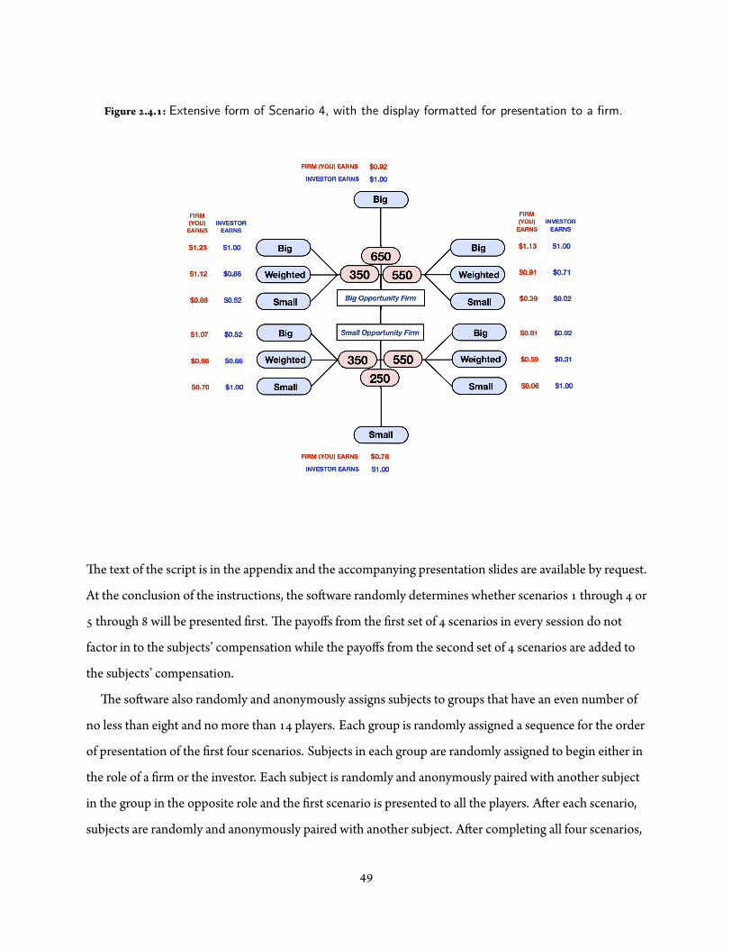
Figure . . : Extensive form of Scenario 4, with the display formatted for presentation to a firm.

e text of the script is in the appendix and the accompanying presentation slides are available by request.

At the conclusion of the instructions, the so ware randomly determines whether scenarios through or

through will be presented rst. e payoffs from the rst set of scenarios in every session do not

factor in to the subjects’ compensation while the payoffs from the second set of scenarios are added to

the subjects’ compensation.

e so ware also randomly and anonymously assigns subjects to groups that have an even number of

no less than eight and no more than players. Each group is randomly assigned a sequence for the order

of presentation of the rst four scenarios. Subjects in each group are randomly assigned to begin either in

the role of a rm or the investor. Each subject is randomly and anonymously paired with another subject

in the group in the opposite role and the rst scenario is presented to all the players. A er each scenario,

subjects are randomly and anonymously paired with another subject. A er completing all four scenarios,

Figure . . : Extensive form of Scenario 8, with the display formatted for presentation to a in-vestor.

subjects swap roles and play the same scenarios in the opposite role, again with random and anonymous

pairings for each scenario. A er completing all four scenarios as both an investor and a rm, subjects are

randomly drawn into new groups and the whole process is repeated for the next four scenarios.

At the start of each round, a er the subject learns whether it will play the role of a rm or an investor

but before the rm’s type is revealed, we present the extensive form of the scenario and ask rms to

identify their anticipated choice if they are assigned to be a “Big” opportunity rm, and their anticipated

choice if they are assigned to be a “Small” opportunity rm. Similarly, investors are asked their anticipated

pricing decisions based on all the alternative store choices that the rm could possibly make for the

current scenario. e rm’s type is then revealed to the rm and the rm can con rm or change their

choice. is choice is then revealed to the investor paired with this rm, and the investor can con rm or

change their price decision. Asking subjects to enter their anticipated decisions prior to revealing the

rm’s type to the rm or the rm’s choice to the investor accomplishes two things. First, it encourages the

subjects to consider the problem from different perspectives before making their nal decision. Second, it

allows us to measure whether rms and investors deviate from their original strategies once information

has been revealed to them.

We lost observations because a technical problem prevented ve subjects from completing all eight

scenarios as a rm. Our nal sample consists of rm-scenario observations.

. . M

Table . . summarizes the variables used in our analysis, Table . . provides summary statistics and

Table . . provides correlations. We create several variables to track information related to the set up of

the game in each round of the experiment. Big is set to ‘ ’ to identify those subjects that are randomly

assigned to have a “Big” opportunity in the current round. Money identi es whether the current round

will affect the subject’s compensation. Session identi es which of the four experimental sessions this

round was run in. Complexity identi es whether the rm is facing greater complexity (i.e., there are three

capacity choices as opposed to two) in the current round or not. Finally,Order is a dummy variable

identifying whether the subject was rst presented with Scenarios through or rst presented with

scenarios through .

We also collect several measures that are generated by the experiment. Undefeated is set to ‘ ’ if the

subject’s choice conforms to what is predicted by the Undefeated re nement, and ‘ ’ if it does not.

Intuitive is set to ‘ ’ if the subject’s choice conforms to what is predicted by the Intuitive Criterion

re nement, and ‘ ’ if it does not. Payoff captures the payoff the subject received in the round, regardless of

whether this amount was added to the subject’s compensation. Switch identi es whether the subject’s

nal choice deviated from the initial strategy they entered prior to learning their type. Finally,Wait tracks

the amount of time the subject waited in the current round. is is in uenced by how long it takes the

other player in the game to make their decision.

We ask participants to complete a post-experiment survey to collect information about their

experience. In particular, we ask “On a scale of - ( : ‘I did not understand the game at all’, : ‘I

understood the game completely’) how well do you feel you understood the game we just played?” From

this response we generate a dummy variable,Understanding, which is set to ‘ ’ if the subject rated their

understanding as a ‘ ’ or higher and ‘ ’ if they rated it a ‘ ’ or lower. We also capture demographic

information in a set of mostly categorical variables – Age,Gender, Ethnicity, Education, Student, ESL

(English as a second language), andMarried.

. . E M

I U R P

We are interested in understanding the relationship between each subject’s self-reported level of

understanding of the game and the likelihood that their decisions are predicted by either the Undefeated

re nement or the Intuitive Criterion re nement. Any predictive power associated with the re nements

could justi ably be called into question if subjects report having a low understanding of the game. We

examine this relationship for the Undefeated re nement by estimating the following model:

Pr(Undefeatedi) = F(β + β · Understandingj + β · Bigi + β · Orderi + β · Switchi+

β ·Moneyi + ξ′Xj + εi),( . )

where subscript i denotes the subject-round observation and j denotes the subject. e vector Xj includes

control variables: Session,Wait, Age,Gender, Ethnicity, Education, Student, ESL, andMarried. To examine

this relationship for the Intuitive Criterion re nement, Intuitive is used as the dependent variable in place

ofUndefeated.

I C R P

We evaluate whether increasing the complexity of the game impacts the likelihood that the outcomes are

predicted by the re nements of interest. We capture the higher complexity construct with Complexity,

which identi es the two scenarios among the eight tested which have three capacity choices as opposed to

two. A er adding Complexity to our speci cation, we estimate the following model:

Pr(Undefeatedi) = F(β + β · Complexityi + β · Understandingj + β · Bigi + β · Orderi+

β · Switchi + β ·Moneyi + ξ′Xj + εi).( . )

I R P

To evaluate whether subjects who make choices that are consistent with the Undefeated re nement or the

Intuitive Criterion re nement earn a higher payoff, we includeUndefeated and Intuitive in the following

speci cation:

Payoff i =γ + γ · Undefeatedi + γ · Intuitivei + γ · Understandingj + γ · Bigi+

γ · Orderi + γ · Switchi + γ ·Moneyi + ξ′Xj + εi.( . )

where Payoff is the realized payoff for the subject in each round. We limit our analysis to scenarios and

since those are the only two scenarios in which both the Undefeated and Intuitive Criterion re nements

have a single predictions that are unique from each other.

. R

Table . . summarizes whether the subjects make choices that are predicted by the Intuitive Criterion or

Undefeated re nements in each of the eight scenarios. From Panel A it is clear that the overwhelming

number of choices do conform with the Undefeated re nement, from a low . for Scenario to a high

of . for Scenario . Panel B, on the other hand, indicates that there is conformance to the Intuitive

Criterion re nement on far fewer occasions, from a low for Scenario to a high of . for Scenario

. Recall that both the Undefeated and Intuitive Criterion re nements predict the same outcome for

Scenarios and , so it is unclear which re nement is driving the results for those scenarios. If Scenarios

and are excluded, the Intuitive Criterion re nement predicts the outcome of the experiment at most

. of the time (Scenario ).

One concern may be that a lack of understanding led to the pa ern of results we observe. Several

features of our experimental design were intended to reduce this possibility, including asking subjects to

enter their strategies before each round of play, having subjects switch roles and play the game both as a

rm and an investor, and including two sets of four scenarios to test for consistent behavior. As discussed

in Section . . , Scenarios through and Scenarios through have a similar structure and the Intuitive

Criterion and Undefeated re nements have the same predictions (refer to Table . . ). e fact that we

get a very similar behavior pa er in Scenarios through and Scenarios through (refer to Table . . )

provides us with some assurance that the subjects understood the game.

We estimate the models in Equations ( . ) and ( . ) using a logistic regression with robust standard

errors clustered by participant. Results are presented as odds ratios. We estimate the model in Equation

( . ) using OLS with with robust standard errors clustered by participant. Tables . . , . . and . .

report the main results from these regressions.

. . I U R P

e results of the logistic regression estimating the speci cation in Equation ( . ) are presented in Table

. . . Models ( ) and ( ) exclude demographic controls while model ( ) and ( ) include them. Models

( ) and ( ) test which variables are associated with the likelihood that the rm’s capacity choice is

consistent with the Undefeated re nement. We estimate Models ( ) and ( ) using observations from

scenarios , , , , , and . For each of these scenarios, the Undefeated re nement has a single

predictions that is different from that predicted by the Intuitive Criterion re nement.

Models ( ) and ( ) test which variables are associated with the likelihood that the rm’s capacity

choice is consistent with the Intuitive Criterion re nement. For both models we excludeOrder as there is

only one observation for which both Intuitive andOrder are non-zero.³ We estimate Models ( ) and ( )

using observations from scenarios and . ese are the only two scenarios for which the Intuitive

Criterion re nement has a single predictions that is different from that predicted by the Undefeated

re nement.

In Model ( ), the odds ratio onUnderstanding is . (SE . , p < . ), indicating that subjects who

indicated a having a high level of understanding about the game were . times as likely to make a capacity

³As a robustness check, we exclude Order from our estimation of Undefeated as well and our inferences do not change(Table . . , Models ( ) and ( )).

choice that was consistent with the Undefeated re nement as subjects who did not have a high level of

understanding. In Model ( ), the odds ratio onUnderstanding is insigni cant (odds ratio . , SE . ,

p > . ) indicating that between those with and without high level of understanding there is no

difference in the likelihood of making a capacity choice consistent with the Intuitive Criterion re nement.

e difference between the coefficients on the impact ofUnderstanding between the two models is

signi cant (Wald χ . , p < . ). Similar results are obtained by comparing models ( ) and ( ). at

our results are robust to the inclusion of controls such as education, age and the use of English as a second

language indicates that the result is not driven by higher aptitude.

We consider other break points on the Likert scale to indicate the subject had a high understanding of

the game, as well capturing their understanding in a more granular categorical variable (not presented)

and our inferences remain unchanged. We cannot use the full -point scale from the original survey

question because the subjects generally indicated they had a high level of understanding of the game (the

mean response using the -point scale was . ), so some of the categories are sparsely populated.

ese results indicate that a high understanding of the game is positively associated with choices

predicted by Undefeated. is is reinforced by noting that the odds ratio on Switch for model ( ) is

signi cant and less than (odds ratio . , SE . , p < . ), indicating that subjects who make a choice

consistent with the Undefeated re nement are much less likely to deviate from the strategy they set prior

to the revelation of their type. is lack of second guessing would naturally correspond to a higher level of

understanding of the game.

. . I C R P

Table . . presents the results of the logistic regression estimating the impact of increased complexity on

the likelihood that the rm’s choices are consistent with either the Undefeated re nement or Intuitive

Criterion re nement. Model ( ) examines the impact of complexity on whether rm choices are

consistent with the Undefeated re nement. We estimate this model using observations from all of the

scenarios since Undefeated re nement has a unique prediction in each scenario. Model ( ) examines the

impact of complexity on whether rm choices are consistent with the Intuitive Criterion re nement. We

estimate this model using observations from scenarios , , , and since these are the only scenarios for

which the Intuitive Criterion re nement results in (at least) one unique PBE. We again excludeOrder as

there is only one observation for which both Intuitive andOrder are non-zero.⁴

Recall that our construct for increased complexity in the rm’s decision is captured by the variable

Complexity, which identi es scenarios which have as opposed to capacity choices. In Model ( ), the

odds ratio on Complexity is . (SE . , p > . ), indicating that scenarios with greater complexity do

not induce the rm to make choices that are more or less consistent with the Undefeated re nement. In

Model ( ), the odds ratio on Complexity is signi cant (odds ratio . , SE . , p < . ) both

statistically and economically. e result indicates that an increase in complexity reduces by a factor of .

the number of rm choices that are consistent with the Intuitive Criterion re nement. e difference

between the coefficients on the impact of Complexity between the two models is signi cant (Wald χ

. , p < . ).

is provides further support that the Undefeated re nement may be more appropriate in many

operations management se ings. Our analysis focuses on relatively constrained decision framework – the

rm has at most three options to choose from. In many operations management decisions the rm has

many more options to choose from. is nding bears further examination to con rm whether even

greater increases in complexity further diminish the predictive power of the Intuitive Criterion

re nement.

. . I R P

Table . . presents the OLS estimation of Equation . specifying the relationship between the subject’s

payoffs and whether their choices are consistent with either the Intuitive Criterion or Undefeated

re nements. Model ( ) excludes demographic controls while Model ( ) includes demographic controls.

We estimate the results for both models using scenarios and , which are the only two scenarios for

which both the Undefeated re nement and the Intuitive Criterion re nement make unique, differentiated

predictions.

In both Models ( ) and ( ) a Wald test comparing the coefficient onUndefeated to the coefficient on

Intuitive indicates that subjects whose choices are predicted my the Undefeated re nement have higher

⁴As a robustness check, we exclude Order from our estimation of Undefeated as well and our inferences do not change(Table . . , Models ( ) and ( )).

payoffs than those whose choices are predicted my the Intuitive Criterion re nement. For model ( ), the

difference in these coefficients is . (Wald χ . , p < . ), while in Model ( ) the difference is

. (Wald χ . , p < . ), indicating that subjects make about . more per round by making

choices consistent with the Undefeated re nement rather than the Intuitive Criterion re nement. is is

somewhat intuitive since the Undefeated re nement relies on choosing PBE based on Pareto dominance

of the payoffs, and it is reassuring to recover this result in an experimental se ing.

. I C

We explore how individuals make decisions relevant in an operations management se ing when there is

information asymmetry between the rm and an outside investor. While stylized models in economics

o en employ assumptions that can abstract from reality, operations management deals with real-world

aspects of decision problems. A common assumption in the signaling game literature is that beliefs among

the participants in the game are re ned using the Intuitive Criterion re nement. rough a series of

experiments, we show that the predictive power of this re nement can be exceptionally low, and that the

Undefeated re nement performs much be er. Importantly, we provide evidence that the subjects making

decisions which aligned with the Undefeated re nement reported a higher understanding of the game

than those who made decisions which aligned with the Intuitive Criterion re nement. ese subjects also

earned higher payouts.

Other experiments have tested the predictive power of re nements with mixed results. To our

knowledge, we are the rst to explicitly perform such tests on the Undefeated re nement, particularly in a

se ing relevant to operations management. Our experimental results reveal that the predictive power of

the Undefeated re nement is robust to increases in the complexity of the decision maker’s choice set,

while that of the Intuitive Criterion re nement deteriorates with greater complexity.

Our results have implications for the burgeoning set of operations research involving information

asymmetry and applications of the Intuitive Criterion re nement. Not only does the Undefeated

re nement predict different outcomes than the Intuitive Criterion re nement in many cases, but the

greater accuracy of those predictions should encourage researchers to include it in future analyses.

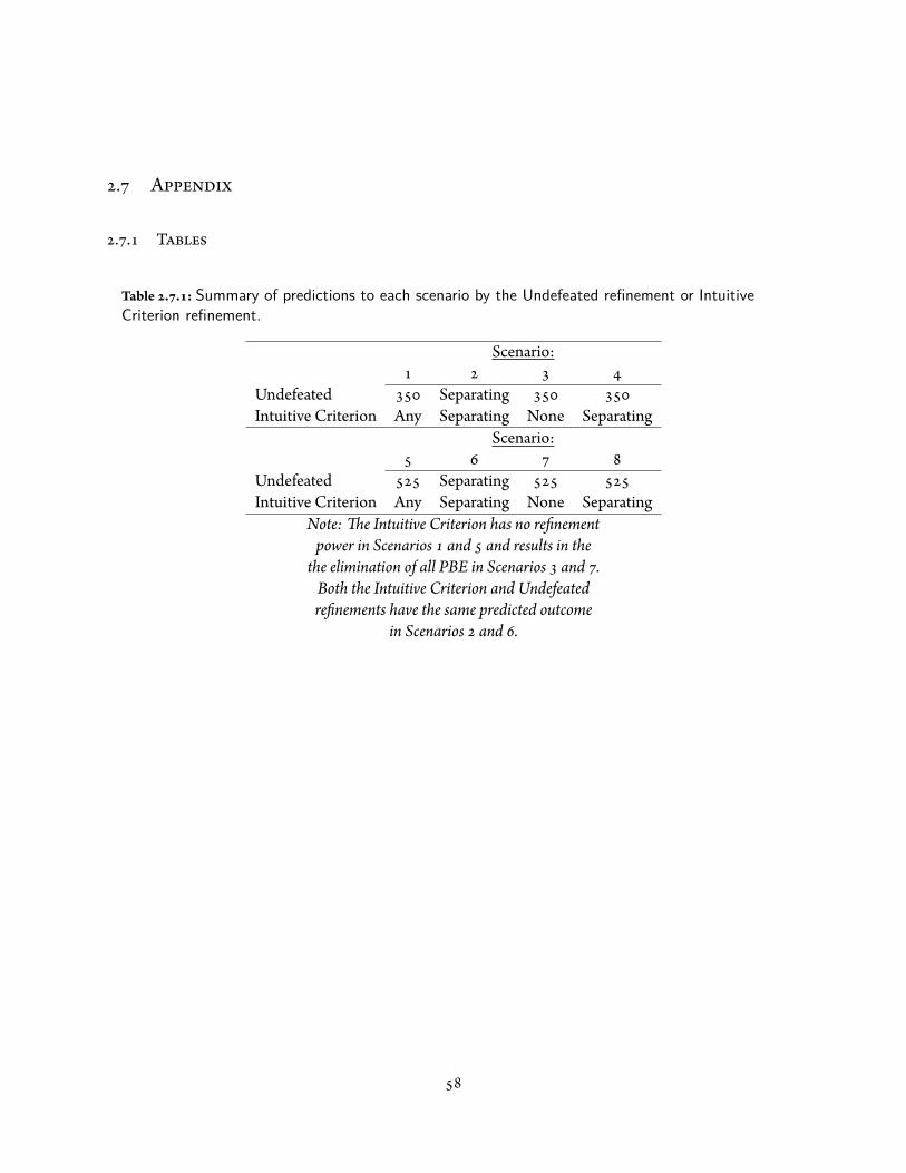
. A

. . T

Table . . : Summary of predictions to each scenario by the Undefeated refinement or IntuitiveCriterion refinement.

Scenario:

Undefeated SeparatingIntuitive Criterion Any Separating None Separating

Scenario:

Undefeated SeparatingIntuitive Criterion Any Separating None Separating

Note: e Intuitive Criterion has no re nementpower in Scenarios and and results in thethe elimination of all PBE in Scenarios and .Both the Intuitive Criterion and Undefeatedre nements have the same predicted outcome

in Scenarios and .

Table . . : Sample summary

Gender Frequency Percent

Male .Female .Missing .Total

Ethnicity Frequency Percent

African American .Asian .Caucasian .Hispanic .Paci c Islander .Missing .Total .

Education A ained Frequency Percent

High school .Some college .Bachelors degree .Masters degree .Missing .Total .

Student Status Frequency Percent

Not a student .Full time student .Part time student .Missing .Total .

Primary Language Frequency Percent

English is primary language .English is secondary language .Missing .Total .

Marital Status Frequency Percent

Not married .Married .Missing .Total .

Table . . : Description of Variables

Variable Description

Undefeated Indicator identifying that the Undefeated re nement predicts the rm’s choice (‘ ’) or not (‘ ’)

Intuitive Indicator identifying that the Intuitive Criterion re nement predicts the rm’s choice (‘ ’) or not (‘ ’)

Payoff Payoff the subject received in the round

Understanding Indicator identifying subject rated their understanding as a ‘ ’ or higher (‘ ’), or a ‘ ’ or lower (‘ ’) on a -point Likert scale

Big Indicator identifying subject is a Big type in current round (‘ ’) or a Small type (‘ ’)

Order Scenarios through were presented to subject st (‘ ’) or scenarios through were presented rst (‘ ’)

Switch Identi es whether the subject’s nal choice deviates from their initial strategy (‘ ’) or not (‘ ’)

Money Earnings from the round was added to the subject’s payout

Session Identi er for the experimental session

Complexity Identi es whether the rm faces three capacity choices (‘ ’) or two capacity choices (‘ ’)

Wait Amount of time the subject waited in the current round

Age Subject’s age

Gender Indicator identifying subject is female (‘ ’) or male (‘ ’)

Ethnicity African-American (‘ ’), American Indian (‘ ’), Asian (‘ ’), Caucasian (‘ ’), Hispanic (‘ ’), Paci c Islander (‘ ’), Other (‘ ’)

continued on the next page

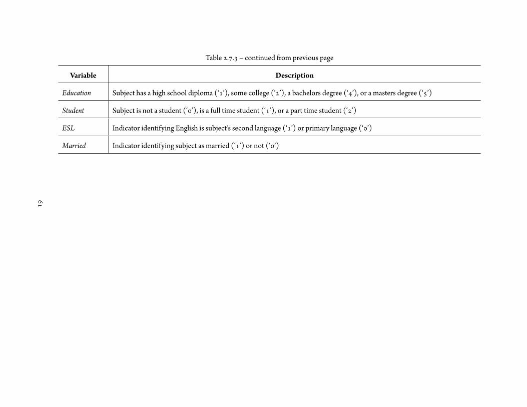
Table . . – continued from previous page

Variable Description

Education Subject has a high school diploma (‘ ’), some college (‘ ’), a bachelors degree (‘ ’), or a masters degree (‘ ’)

Student Subject is not a student (‘ ’), is a full time student (‘ ’), or a part time student (‘ ’)

ESL Indicator identifying English is subject’s second language (‘ ’) or primary language (‘ ’)

Married Indicator identifying subject as married (‘ ’) or not (‘ ’)

Table . . : Summary Statistics

Variable Mean Std. Dev. Min. Max. NUndefeated . .

Intuitive . .

Payoff . . .

Understanding . .

Big . .

Order . .

Switch . .

Money . .

Session . .

Complexity . .

Wait . .

Age . .

Table . . : Correlations

Variables Und

efea

ted

Intu

itive

Payo

ff

Und

erstan

ding

Big

Ord

er

Switc

h

Mon

ey

Sessio

n

Com

plex

ity

Wait

Age

Undefeated .Intuitive . .Payoff . - . .Understanding . - . . .Big - . - . . . .Order - . . - . . . .Switch - . . - . . - . . .Money . - . . . . - . - . .Session - . . - . . . . . . .Complexity - . - . . - . . - . . - . - . .Wait . . . - . - . - . - . . - . - . .Age - . . - . - . . - . - . - . - . - . - . .

Table . . : Summary of whether subject choices made decisions which conformed to predictions ofthe Undefeated refinement or Intuitive Criterion refinement in each scenario.

Panel A. Does the subject’s choice conform with that predicted by the Undefeated re nement?Scenario:

* * TotalNo

. . . . . . . . .Yes

. . . . . . . . .Total

Panel B. Does the subject’s choice conform with that predicted by the Intuitive Criterion?Scenario:

* * TotalNo

. . . . .Yes

. . . . .Total

*Both the Intuitive Criterion and Undefeated re nements have the same predicted outcome in Scenarios and .e Intuitive Criterion has no re nement power in Scenarios and and results in the elimination of all PBE in

Scenarios and .

Table . . : Estimating whether the subject’s choice is consistent with the Undefeated refinementor the Intuitive Criterion refinement.

Dependent Variable:Undefeated Intuitive Undefeated Intuitive

( ) ( ) ( ) ( )

Understanding . * . . * .[ . ] [ . ] [ . ] [ . ]

Big . . * . . *[ . ] [ . ] [ . ] [ . ]

Order . * . *[ . ] [ . ]

Switch . ** . + . ** .[ . ] [ . ] [ . ] [ . ]

Money . + . . + .[ . ] [ . ] [ . ] [ . ]

Constant . * . . ** .[ . ] [ . ] [ . ] [ . ]

ObservationsPseudo R . . . .Mean DV . . . .Pearson χ . . . .Pearson p-value . . . .Wald χ . * . *Wald p-value . .

Notes: Logistic estimation with results presented as odds ratios. Robust standard errors clustered bysubject in brackets. Models ( ) and ( ) are estimated using scenarios , , , , and and includecontrols Session andWait. Models ( ) and ( ) are estimated using scenarios and and also includecontrols Age,Gender, Ethnicity, Education, Student, ESL, andMarried. Pearson χ and Pearson p-value

assess the goodness of t of the model. Wald χ and Wald p-value provide a test of the equivalency of thecoefficient onUnderstanding across models ( ) and ( ), and models ( ) and ( ). ** p< . , * p< . , +

p< .

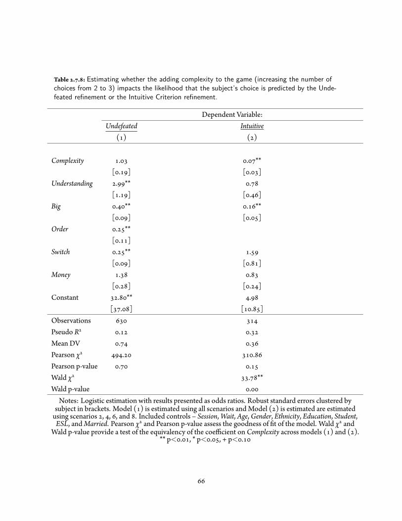
Table . . : Estimating whether the adding complexity to the game (increasing the number ofchoices from 2 to 3) impacts the likelihood that the subject’s choice is predicted by the Unde-feated refinement or the Intuitive Criterion refinement.

Dependent Variable:Undefeated Intuitive

( ) ( )

Complexity . . **[ . ] [ . ]

Understanding . ** .[ . ] [ . ]

Big . ** . **[ . ] [ . ]

Order . **[ . ]

Switch . ** .[ . ] [ . ]

Money . .[ . ] [ . ]

Constant . ** .[ . ] [ . ]

ObservationsPseudo R . .Mean DV . .Pearson χ . .Pearson p-value . .Wald χ . **Wald p-value .

Notes: Logistic estimation with results presented as odds ratios. Robust standard errors clustered bysubject in brackets. Model ( ) is estimated using all scenarios and Model ( ) is estimated are estimatedusing scenarios , , , and . Included controls – Session,Wait, Age,Gender, Ethnicity, Education, Student,ESL, andMarried. Pearson χ and Pearson p-value assess the goodness of t of the model. Wald χ and

Wald p-value provide a test of the equivalency of the coefficient on Complexity across models ( ) and ( ).** p< . , * p< . , + p< .

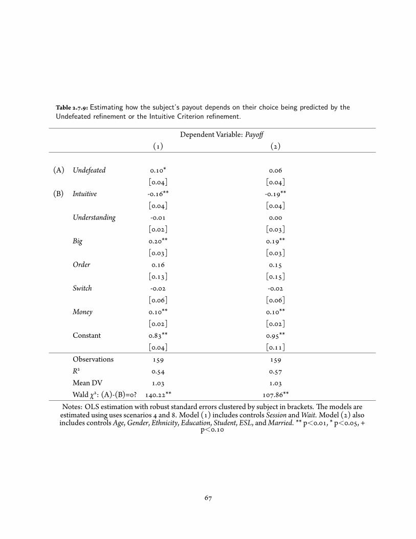
Table . . : Estimating how the subject’s payout depends on their choice being predicted by theUndefeated refinement or the Intuitive Criterion refinement.

Dependent Variable: Payoff( ) ( )

(A) Undefeated . * .[ . ] [ . ]

(B) Intuitive - . ** - . **[ . ] [ . ]

Understanding - . .[ . ] [ . ]

Big . ** . **[ . ] [ . ]

Order . .[ . ] [ . ]

Switch - . - .[ . ] [ . ]

Money . ** . **[ . ] [ . ]

Constant . ** . **[ . ] [ . ]

ObservationsR . .Mean DV . .Wald χ : (A)-(B)= ? . ** . **

Notes: OLS estimation with robust standard errors clustered by subject in brackets. e models areestimated using uses scenarios and . Model ( ) includes controls Session andWait. Model ( ) alsoincludes controls Age,Gender, Ethnicity, Education, Student, ESL, andMarried. ** p< . , * p< . , +

p< .

Table . . : Estimating whether the subject’s choice is consistent with the Undefeated refinementor the Intuitive Criterion refinement.

Dependent Variable:Undefeated Intuitive Undefeated Intuitive

( ) ( ) ( ) ( )

Understanding . ** . . + .[ . ] [ . ] [ . ] [ . ]

Big . ** . ** . . *[ . ] [ . ] [ . ] [ . ]

Order . ** . *[ . ] [ . ]

Switch . ** . . * .[ . ] [ . ] [ . ] [ . ]

Money . . . + .[ . ] [ . ] [ . ] [ . ]

Constant . ** . . .[ . ] [ . ] [ . ] [ . ]

ObservationsPseudo R . . . .Mean DV . . . .Pearson χ . . . .Pearson p-value . . . .Wald χ . * . *Wald p-value . .

Notes: Logistic estimation with results presented as odds ratios. Robust standard errors clustered bysubject in brackets. eUndefeated dependent variable in column ( ) uses all scenarios while column ( )uses scenarios and . e Intuitive dependent variable in column ( ) uses scenarios , , and while

column ( ) uses scenarios and . Models ( ) and ( ) include controls Session andWait. Models ( ) and( ) also include controls Age,Gender, Ethnicity, Education, Student, ESL, andMarried. Pearson χ andPearson p-value assess the goodness of t of the model. Wald χ and Wald p-value provide a test of theequivalency of the coefficient onUnderstanding across models ( ) and ( ), and models ( ) and ( ). **

p< . , * p< . , + p< .

Table . . : Robustness tests on the impact of Understanding and Complexity after removingOrder from specifications with Undefeated as a dependent variable

Dependent Variable:Undefeated Intuitive Undefeated Intuitive

( ) ( ) ( ) ( )

Complexity . . **[ . ] [ . ]

Understanding . * . . ** .[ . ] [ . ] [ . ] [ . ]

Big . + . * . ** . **[ . ] [ . ] [ . ] [ . ]

Switch . ** . . ** .[ . ] [ . ] [ . ] [ . ]

Money . ** . . * .[ . ] [ . ] [ . ] [ . ]

Constant . ** . . ** .[ . ] [ . ] [ . ] [ . ]

ObservationsPseudo R . . . .Mean DV . . . .Pearson χ . . . .Pearson p-value . . . .Wald χ . .Wald p-value . .

Notes: Logistic estimation with results presented as odds ratios. Robust standard errors clustered bysubject in brackets. eUndefeated dependent variable in column ( ) uses game types , and ; whilecolumn ( ) uses all game types. e Intuitive dependent variable in column ( ) uses game type whilecolumn ( ) uses game types and . Included controls – Session,Wait, Age,Gender, Ethnicity, Education,Student, ESL, andMarried. Pearson χ and Pearson p-value assess the goodness of t of the model. Waldχ and Wald p-value provide a test of the equivalency of the coefficient onUnderstanding across models( ) and ( ), and test of the equivalency of the coefficient on Complexity across models ( ) and ( ). **

p< . , * p< . , + p< .

. . S I S

e script read to all subjects in the experiment is below. A copy of the presentation slides that

accompany the script are available upon request from the authors.

Slide . Welcome. I will rst take you through an overview of the game that you will play and then

walk you through an example that will describe exactly how you will play this game on the computer.

Slide . You will be randomly assigned to play the role of either a Firm or an Investor. Firms and

Investors will then be randomly and anonymously paired with different people in each round.

Slide . Firms will either have a “Small” or “Big” market opportunity, which is just the number of

customers the Firm expects to have for its product or service. Both the Firm and Investor will know the

Firm’s likelihood of ge ing a “Small” or “Big” market opportunity, but only the Firm will know for sure its

actual opportunity.

Slide . Knowing its market opportunity, the Firm will decide how many stores to open. e Firm’s

payoff depends not only on this decision, but on the price the Investor sets for the Firm.

Slide . e Investor learns how many stores the Firm will open and sets a price for the Firm. e

Investor’s payoff depends on se ing a price close to the Firm’s actual value.

Slide . You will see a picture similar to this in each game you play. I will cover the information on this

picture.

As I mentioned previously, in each round the Firm is randomly assigned either a “Big” market

opportunity or a “Small” market opportunity.

Slide . Here the Firm has three choices for the number of stores to open, depending on its market

opportunity. is is the most complex situation you will see. You will also see situations in which only

two of three choices are available. In this example, a “Big” opportunity Firm can choose to open ,

or stores while a “Small” opportunity Firm can choose to open , , or stores. Note that your

information is always in red and the other player’s information is in blue.

Slide . Depending on the Firm’s choice, the Investor has either no choice or three choices for what

price to set for the Firm. In this example, only a Firm with a “Big” opportunity can open stores, and

only Firm with a “Small” opportunity can open stores. Note that both a “Big” and a “Small”

opportunity Firm can open either or stores. If the Investor sees one of these choices the Investor

must decide whether to set a “Big”, “Small” or “Weighted” price to the Firm. A “Weighted” price is simply

a weighted average price.

Slide . If you are a Firm, your payoff depends on the size of the opportunity, your store choice, and

the price the Investor sets. In this example, if a “Big” Firm chooses stores it will get a payoff of . .

If, however, a “Big” Firm chooses stores it will get a payoff of either . , . or . depending

on whether the Investor sets a price of “Big”, “Weighted” or “Small”. Similarly, if a “Big” Firm chooses

stores it will get a payoff of either . , . or . depending on whether the Investor sets a price of

“Big”, “Weighted” or “Small”.

Slide . If you are an Investor, your payoff depends on se ing a price close to the Firm’s actual value.

For instance, in this example if the Firm chooses stores and the Investor sets a price of “Big”, the

Investor will receive a payoff of . if the Firm is “Big,” and a payoff of . if the Firm is instead “Small”.

Slide . When the game begins, you will be told on screen whether you are a Firm or an Investor and

the chance the Firm has of ge ing a “Big” or “Small” market opportunity. You will see a graphic with the

choices and payoffs for your game. Firms and Investors will receive the same information and will be

asked to de ne their strategies. If you are a Firm, you will be asked “If you faced a Big market opportunity,

how many stores would you open?” and “If you faced a Small market opportunity, how many stores would

you open?”

Slide . If you are an Investor, you will be asked “If the Firm opened X stores, what price would you

give them?”

Slide . e Firm’s market opportunity is then randomly assigned and the Firm con rms their store

quantity choice.

Slide . e Investor sees the Firm’s store quantity choice and con rms the price they want to give to

the Firm.

Slide . e Firm and Investor learn what their pay-outs are for the previous game. Firms and

Investors are randomly assigned to new partners, Firms are randomly assigned a “Big” or “Small”

opportunity and a new game begins with different choices. A er a few games, Firms and Investors will

swap roles.

Slide . e rst several rounds will be practice rounds and the next several rounds will be for

money. We will make it clear when you are playing for money. In addition to your show-up fee, you will

be paid the sum of all your individual payoffs from the money rounds at the end of today’s session.

You should try to make as much money as possible. You are not taking money from other players.

You are playing with other people, and they can’t move forward unless you move forward. Please make

your decisions in a timely fashion�be thoughtful but move quickly.

If your screen is black it means you are waiting for another player to make a decision.

Please don’t close your browser, or press next, back or refresh on the browser, as this can disrupt the

game. If you have any questions during the practice rounds, please raise your hand, and one of us will

come around and answer your question. ank you! You may now begin.

. . E F R

Figure . . : Extensive form of Scenarios 1 and 5.

(a)Firm and investor payoffs for Scenario 1.Display of information is formatted for a firm.

(b)Firm and investor payoffs for Scenario 5.Display of information is formatted for aninvestor.

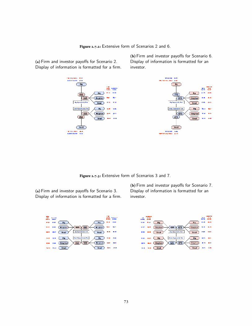
Figure . . : Extensive form of Scenarios 2 and 6.

(a)Firm and investor payoffs for Scenario 2.Display of information is formatted for a firm.

(b)Firm and investor payoffs for Scenario 6.Display of information is formatted for aninvestor.

Figure . . : Extensive form of Scenarios 3 and 7.

(a)Firm and investor payoffs for Scenario 3.Display of information is formatted for a firm.

(b)Firm and investor payoffs for Scenario 7.Display of information is formatted for aninvestor.

3Managerial Discretion and theMarket’s Re onse to

Supply ChainDisruptions

. I

Anecdotal and empirical evidence indicates that supply chain disruptions affect rm performance. Such

disruptions have also been found to be extremely damaging to rm value, reducing the value of the rm’s

common equity on average in excess of (Hendricks and Singhal , World Economic Forum and

Accenture ). While it is not surprising that a disruption to a company’s supply chain or operations

can impose costs on the company and affect its market value, the magnitude of the impact identi ed in the

literature is incredible. Surprisingly, no research has currently examined whether this potential market

response induces management to behave strategically in deciding whether or not to reveal disruptions.

is is the focus of our research.

We examine whether managers exercise signi cant discretion in disclosing material disruptions to the

market, and whether such actions are related to the market’s response either through a selection effect or a

treatment effect. We gain insight into these issues by taking advantage of a change in U.S. securities

regulations. Section of the Sarbanes Oxley Act of (SOX), implemented during the sample

period, compels rms to promptly disclose events that may impair their operations or nancial condition.

We utilize the enforcement of Section as an exogenous policy shock in our model. Our empirical

ndings and interviews with current and former executives provide evidence that, prior to the regulatory

change, managers exercised signi cant discretion in the disclosure of material disruptions.

We also use SOX Section to analyze whether changes in managerial discretion in uences the

relationship between the announcement of a disruption and the stock market’s response. In keeping with

prior empirical studies, we nd a negative impact on company value that is statistically signi cant and

economically meaningful. We nd, however, that the impact is considerably smaller a er the new

disclosure laws go into effect. We cannot conclusively determine whether this is a selection effect

(managers failing to disclose material disruptions), a treatment effect (the markets responding more

favorably to disruptions based on the knowledge that there is less information asymmetry with the rm),

or both. We run a series of robustness tests which provides some evidence that both factors may be at play.

. L R

We build on the literature dealing with supply-chain risk management, principally those studies

examining the impact of disruptions on rms and their stakeholders. Supply-chain risk management

remains a nascent area of academic research, characterized by diverse viewpoints on the scope of the eld

and on appropriate analytical methodologies (Sodhi et al. ). ere is abundant evidence, however,

that disruptions can have a material and negative impact on company performance (Hendricks and

Singhal , a,b, Sheffi , World Economic Forum and Accenture ), and emerging research

that explores how rm actions or characteristics may mitigate the impact of disruptions. Braunscheidel

and Suresh ( ) use survey results to investigate whether features of the rm’s culture and

organizational integration practices are associated with the agility with which the rm’s management

responds to disruptions. Kleindorfer and Saad ( ) provide evidence that changes to risk assessment

and risk mitigation practices reduced the impact of disruptions in the chemical industry.

Another stream of research considers how rms can coordinate with their suppliers to minimize the

impact of disruptions. Tomlin ( ) provides some theoretical insight on this question by developing a

model of a single product rm that can source from two suppliers – one that is reliable but more expensive

than the second, less reliable supplier. e author nds that characteristics of disruptions, such as the

frequency and duration, affect the rm’s outcomes and should therefore in uence the rm’s optimal

sourcing strategy. Tang ( ) theorizes that rms may be able to in uence their vulnerability to

disruptions by adopting different supply-chain strategies (including postponement, and storing inventory

at strategic locations). Christopher and Lee ( ) assert that disruption risks can be mitigated by

developing mutual con dence among the participants in the supply chain. Using qualitative ndings from

phone interviews and focus groups, Craighead et al. ( ) propose that supply-chain density,

complexity and node criticality contribute to the severity of disruptions, and that the ability to quickly

disseminate information within the supply chain dampens the severity of disruptions.

Our analysis differs from and builds on this literature in two ways. We are the rst to consider in the

empirical literature whether managers act strategically in their decision to disclose disruptions to their

investors. We also explore whether such strategic disclosure in uences the impact of disruptions on rm

value.

. T H

. . M D A D

Managers have a well-established responsibility to disclose material information about the rm’s

condition to investors. By the early ’s, many U.S. stock exchanges had instituted disclosure

requirements as a prerequisite for listing a rm’s securities (Berle and Means ). Federal legislation

dating back to the Securities Act mandated that managers disclose material information that a

reasonable investor would require to make an investment decision (Simon ). e bene ts of

reducing information asymmetry with the investors is such that many rms voluntarily enlisted nancial

intermediaries, including external auditors, to provide credible information to investors well before the

passage of federal laws requiring this practice (Easterbrook and Fischel ).

When rms do experience negative events, their managers face a number of incentives to disclose such

information to investors, including advantaging their rm’s securities in both the primary and secondary

markets by alleviating information asymmetries, and avoiding legal liability if they failed to make

disclosures (Easterbrook and Fischel ). Managers might also face reputational damage and expose

themselves and their rms to regulatory and legal action if they do not disclose material information.

Gigler and Hemmer ( ) capture some of these forces in a model that shows that managers will

voluntarily disclose material information even before a mandatory nancial reporting deadlines.

Investors also have an interest in exerting pressure on management to adopt timely disclosure practices

because such practices afford protection in an otherwise riskier capital market (Suphap ). High

quality disclosure also leads to greater market efficiency as more information can be processed by

investors and analysts, the cost of redundant data collection efforts is reduced, and capital can be allocated

more effectively with improved information (Coffee ). In sum, managers and investors have strong

mutual incentives to ensure that the rm is disclosing all material information (Coffee ).

Any problems with timely information disclosure, if they do exist, may also be isolated to speci c

instances rather than re ective of broad managerial practice. In spite of high-pro le cases of managerial

misconduct, recent federal laws expanding the regulatory mandate of the Securities and Exchange

Commission (SEC) have been criticized as a questionable and potentially unnecessary regulatory

intervention to address an isolated problem (Coates , Hart ). Critics claim that these laws are an

overreaction to a very small number of bad actors who are not representative of a systemic problem, and

that existing regulations already provide remedies to punish (and thus broadly deter) corporate

malfeasance. As pointed out by Coates ( ), the criminal prosecutions at Enron, Tyco and Worldcom

were all based on laws that had been on the books for decades.

Finally, even if managers had been systematically failing to disclose material information about

operational disruptions, enhanced disclosure rules might result in the opposite behavior than they intend,

by reducing rather than expanding the dissemination of information. e SEC reported that several

respondents to their proposal for fair disclosure rules indicated that rms “would nd it so difficult to

determine when a disclosure of information would be ‘material’ (and therefore subject to the regulation)

that, rather than face potential liability and other consequences of violating Regulation FD, they would

cease informal communications with the outside world altogether” (Securities and Exchange

Commission ).

Despite these regulatory traditions and desires by many stakeholders for disclosure to promote

efficient markets, managers actually possess considerable discretion about whether and when to disclose

material disruptions. e SEC has declined to articulate a “bright-line standard” identifying what

constitutes material information (Securities and Exchange Commission ). Since disruptions erode

pro ts and investor con dence, they can reduce rm value in the short run. Managers’ pecuniary

incentives, including stock options and performance bonuses, can deter them from disclosing such

problems. Managers may also be hesitant to disclose problems out of fear that competitors will seek to

capitalize on the information, or customers will use it as leverage in future negotiations.

As we describe in Section . . , the SEC introduced new regulations related to SOX Section which

expanded the set of required corporate disclosures and shortened disclosure deadlines. While the new

disclosure requirements had li le to do with operational disruptions, they forced companies to streamline

and formalize their disclosure practices generally. Consequently, management’s ability to exercise

discretion on whether or not to reveal operational disruptions should be reduced.

Hypothesis Managers exercise signi cant discretion in the disclosure of material disruptions and such

discretion is alleviated by more formalized corporate disclosure rules.

. . I D I D

If managers do not reveal all material disruptions, it may be that they are selecting which disruptions to

reveal based on their perception of the impact of such disclosures on the rm’s share price. Whether they

are in uenced to conceal disruptions that are more or less damaging to rm value is not clear ex ante. For

instance, managers may have pecuniary incentives in the form of stock options, bonuses and career

advancement that may induce them to avoid revealing those disruptions which are likely to have the

greatest adverse impact on the rm’s stock price. Such disruptions, however, are also apt to be more

difficult for the rm to address discreetly, thus providing greater incentive for managers to disclose them

and thereby avoid the appearance of obfuscation. Managers may not want to risk losing investor goodwill

or other reputational bene ts by a empting to hide a material disruption.

ere is empirical evidence in the accounting literature suggesting that there is a selection effect in

managerial disclosure decisions, but the evidence is con icting as to whether managers avoid releasing

bad news or not.¹ Kothari et al. ( ) analyze the release of earnings forecasts and dividend changes and

nd that managers delay the release of bad news relative to good news. Skinner ( ), however, provides

evidence in the se ing of quarterly nancial reporting that managers are more likely to preemptively

disclose extremely bad earnings information in advance of regular earnings releases as opposed to mildly

disappointing earnings information. Earnings information and dividend changes differ from supply chain

disruptions not only because they are subject to standardized reporting and third-party auditing but also

because their disclosure may be less prone to managerial discretion. It is therefore unclear whether

management will behave in a similar fashion for supply chain disruptions.

It is also unclear whether a treatment effect exists between greater disclosure and market returns, and if

so, what direction it takes. Prompt disclosure could reduce information asymmetry between rm and

investor, creating more goodwill with the investors and alleviating the stock market’s response to

disruptions. Greater disclosure may also desensitize investors and dilute the informational value of

disclosures (Lawrence and Prentice ). On the other hand, prompt disclosure gives less opportunity

for news to leak out prior to disclosure, resulting in a larger response to the disclosure because it contains

new information.

We hypothesize that the dominate effect will be that greater disclosure is associated with a milder

market response to disruptions.

Hypothesis Greater disclosure of disruptions is associated with an amelioration of the impact of such

disruptions on rm value.

. . A D I E F

Commonly applied models of determining the value of a rm involve forecasting the rm’s future stream

of cash ows and discounting those cash ows using an appropriate risk adjusted rate (Brealey et al.

¹For an overview of the empirical literature on corporate disclosure, see Healy and Palepu ( ).

). Such models highlight that disruptions may impact rm value by affecting the cash thrown off by

the rm’s operations and / or by increasing the riskiness of those cash ows. Prior research has shown that

on average disruptions are associated with lower future rm performance, including lower growth in sales

and higher growth in costs (Hendricks and Singhal a). If some types of disruptions are associated

with comparatively worse future performance or increased risk, it can be expected that they will also have

a more negative impact on rm value. is may occur either because a disruption is itself more costly or

because the disruption portends riskier operations due to a greater likelihood of future disruptions.

We consider these effects by characterizing disruptions as either internal to the rm, internal to the

rm’s supply chain, or environmental. One intuitive premise in cross-organizational coordination and

control in organizational theory (Powell , Sco and Davis ) and more speci cally in the

operations management literature (Chopra and Meindl , Kok and Graves ) is that rms exercise

more control over their operations and supply chain than over the environment. Disruptions that are

internal to the rm or its supply chain may be perceived as being are at least partially under the rm’s

presumptive control. Such a disruption may signal to the market that something is wrong with the rm’s

internal control mechanisms such that future disruptions, and hence either lower cash ows or higher

systematic risk, may be more likely. ere is some empirical support for such a nding. Hammersley et al.

( ) found that when rms preemptively disclose internal accounting control weaknesses related to

nancial reporting it elicits a negative price reaction from the stock market.

Disruptions a ributed to environmental factors, on the other hand, can be perceived as random or

events over which the rm is not expected to be able to exert much control. Consequently, environmental

disruptions are less likely than internal disruptions to signal that something is wrong with the rm’s

internal controls or that the rm’s operations are fragile.

Hypothesis Disruptions that are outside the rm’s control will have a milder impact on rm value than will

disruptions that are a ributed to factors internal to the rm.

. D E M

. . S

In identifying observations for the analysis, we adopt the Craighead et al. ( , pg. ) de nition of

disruptions as “unplanned and unanticipated events that disrupt the normal ow of goods and materials

within a supply chain and, as a consequence, expose rms within the supply chain to operational and

nancial risks.” For instance, in a manufacturing environment, disruptions include events such as an

unscheduled plant shutdown, a parts shortage, and a transportation interruption. In a retail environment,

disruptions include events such as supplier and logistics failures.

We identify disruptions by reviewing company press releases distributed via the PRNewswire and

Business Wire because press releases are widely recognized as a common and effective means for

companies to transmit information to shareholders and other constituents in a timely fashion. In issuing

its nal rule on Regulation FD (Fair Disclosure), the SEC encouraged companies to use press releases as

the rst step in a three-step process to ensure the broad dissemination of material non-public information.

“We believe that issuers could use the following model, which employs a combination of methods of

disclosure, for making a planned disclosure of material information, such as a scheduled earnings

release. First, issue a press release, distributed through regular channels, containing the

information; second, provide adequate notice, by a press release and/or website posting, of a

scheduled conference call to discuss the announced results, giving investors both the time and date

of the conference call, and instructions on how to access the call; and third, hold the conference call

in an open manner, permi ing investors to listen in either by telephonic means or through Internet

webcasting. By following these steps, an issuer can use the press release to provide the initial broad

distribution of the information, and then discuss its release with analysts in the subsequent

conference call, without fear that if it should disclose additional material details related to the

original disclosure it will be engaging in a selective disclosure of material information. We note that

several issuer commenters indicated that many companies already follow this or a similar model for

making planned disclosures” (Securities and Exchange Commission ).

e SEC also noted that in many cases self-regulatory organization rules already require companies to

issue press releases to announce material developments.

To generate our sample, we apply a search string to the Factiva database of press releases from January

, , until December , . is search string identi es announcements in which the headline or

lead paragraph includes such terms as delay, disruption, interruption, shortage, or problemwithin words of

terms like component, delivery, parts, shipment, manufacturing, production, or operations. Of the

approximately . million press releases in the Factiva database during our study period, the search string

returns approximately , press releases. We manually reviewed these announcements for relevance.

Common reasons why press releases were disquali ed in the manual-review stage include that they did

not pertain to an actual disruption or pertained to a previously announced disruption. e manual review

process yielded press releases representing the rst announcement of an actual disruption. From this

set of press releases, we linked of them to rms with the requisite nancial information for

the analysis of whether disruptions are routinely disclosed. Of these, announcements from rms

also had the requisite stock price information for the analysis on the impact of increased disclosure on

company valuation. Characteristics of the disruption announcements are reported in Table . . .

Approximately one-third of the disruption announcements include earnings information in the form of

updated earnings forecasts or full earnings releases. Simply dropping those announcements that contain

contemporaneous earnings information may distort the measured impact on rm value of disruptions.

Instead, we seek to use this additional information to examine the impact on rm value of disruptions

which exceeds their effect through earnings. In addition, this information allows us to control for the fact

that some types of disruptions are simply larger than other types of disruptions, which is particularly

important in our test of Hypothesis . So that we can robustly control for the impact of earnings

information on rm value, we augment each disruption announcement with announcements of that rm’s

quarterly nancial performance for one year before and one year a er the disruption date. e nal data

set includes , earnings-only announcements, resulting in a total of , announcement

observations. We link the information from the press releases and earnings announcements to rm stock

price information from the Center for Research in Security Prices (CRSP) database, rm nancial

performance information from the Standard and Poor’s COMPUSTAT database, and rm earnings

expectations from the Institutional Brokers’ Estimate System (I/B/E/S) database.

C A

From each announcement we extract the company name, company identifying information,

announcement date, earnings information (if provided), and the source of the disruption (for

disruption-related announcements). We classify the source of the disruption as either internal, external, or

environment. A disruption is classi ed as internal if it is a ributed in the announcement to the rm’s

internal operations, including its staff or facilities. A disruption is classi ed as external if it is a ributed to

the rm’s suppliers, including inbound or outbound logistics and transportation providers. A disruption

is classi ed as environment if it is a ributed factors outside the rm and its supply chain, including

weather, government regulations, natural disasters, and political turmoil. Disruptions are classi ed by

their root cause. For instance, if an earthquake disrupts a rm’s critical supplier then the disruption is

classi ed as environment. If instead the supplier is disrupted by an mechanical problem at its plant, then

the disruption is classi ed as external. Disruption are classi ed to multiple causes in an isolated number of

cases when the announcement makes clear that more than one cause played an important role. We run a

robustness test that randomly classi es each of these disruptions to single sources and the inferences from

our analysis are unaffected.

. . R R E D

S O S

Central to our analysis is the enforcement date of regulations enacted to ensure corporate compliance

with the Public Company Accounting Reform and Investor Protection Act, also known as the

Sarbanes-Oxley (SOX) Act. Congress passed SOX in July a er a series of notorious corporate

scandals involving companies such as Adelphia, Enron, and Worldcom. e SEC formalized a series of

additions and changes to existing regulations in response to this new legislation.² e regulations of

primary interest to us are those intended to comply with the real time disclosure mandate in Section

of SOX. is Section requires rms to “disclose to the public on a rapid and current basis such additional

information concerning material changes in the nancial condition or operations of the issuer” ( th

Congress ). e SEC issued a nal ruling on the new regulations related to Section in March

²See “Spotlight on Sarbanes-Oxley Rulemaking and Reports” h p://www.sec.gov/spotlight/sarbanes-oxley.htm

that had an effective date of August , .

Two aspects of these rules are particularly relevant to our study. First, the SEC shortened the deadline

for disclosure of most items on the Form -K to four business days a er the occurrence of a triggering

event, down from ve to een days that was previously in place for different types of events.³ Second, the

SEC also introduced new disclosure requirements for a wider range of corporate events, but it did not

change the scope for the disclosure of operational and nancial results. To accommodate the increase in

the number of disclosable events, the SEC introduced a new format for the Form -K. Since there were no

changes to the disclosure of operational and nancial results, however, it retained in Item . of the new

Form -K all of the requirements regarding the public announcements of material non-public information

of a company’s results of operations or nancial condition which had been included in former Item of

the old Form �K. e SEC did, however, expand the set of other types events that rms must disclose.

For a list of the changes made to the list of events which must be disclosed on the Form -K, see Table

. . in the Appendix.

In making their nal ruling, the SEC emphasized that the new regulations provide for be er and more

timely disclosure of important corporate events, moving towards a system emphasizing current reporting.

It also pointed out the presumptive bene ts on the markets of faster disclosure, stating that,

“Under the prior system, predicated primarily on a periodic reporting system, the securities of a

company could be trading on less complete information if an important corporate event has

occurred but the company, under no duty to report that event, does not report the event on a timely

basis. Such a delay in disclosure permits there to be signi cant time periods during which

important information is not disclosed to the market. ese circumstances create opportunity for

companies and those with access to non-public information to misuse that information. e

amendments adopted today will reduce such opportunities for misuse” (Securities and Exchange

Commission ).

e new rules were intended to identify those events which are “unquestionably or presumptively

material events that must be disclosed currently,” but not to change the threshold for what constitutes a

³ e SEC introduced the Form -K in and it provides a mechanism for companies to report material corporateevents to the SEC on a more current basis than either the Forms -K and -Q, which are used to le annual and quarterlyreports (see h p://www.sec.gov/answers/form k.htm).

material event (Securities and Exchange Commission ). e regulation neither sets nor refers to a

de nition for materiality. In fact, the SEC has consistently avoided developing a bright line rule for

materiality and instead has relied on existing case law (Securities and Exchange Commission ).

SOX S A F S

Another signi cant set of regulations, those pertaining to the enforcement of SOX Section , took

effect nearly concurrent with the regulations related to Section . We will take advantage of this

happenstance in our analysis to shed some light on whether the relationships we uncover are the result of

greater awareness of disruptive events or changes in managerial discretion in reporting those events.

Section of SOX requires the rm’s management to include an internal control report with the rm’s

annual report that affirms “the responsibility of management for establishing andmaintaining an adequate

internal control structure and procedures for nancial reporting,” and provides an assessment “of the

effectiveness of the internal control structure and procedures of the issuer for nancial reporting” ( th

Congress ). e SEC adopted nal rules on June , in response to this section of SOX. ese

rules require that beginning in with the rm’s scal year ending on or a er July , , rms include a

report on the company’s internal control over nancial reporting which includes a statement from

management that they acknowledge their responsibility in establishing and maintaining such controls, an

assessment of the effectiveness of those controls, a description of the framework use to make that

assessment, an evaluation of any changes which would affect those controls, and an a estation on

management’s assessment from the rm’s external auditor (Securities and Exchange Commission ).

e cost and effort associated with complying with the new Section requirements is substantial. In

a survey of over companies, Ernst and Young found that over undertook signi cant remediation

of core business operations prior to a aining initial compliance, over of companies with annual

revenues in excess of billion invested more than , staff hours in activities related to Section

, of companies with annual revenues between and billion in invested more than million

in initial SOX section compliance, and deployed or intended to deploy an enterprise risk

management system within one year of initial compliance (Ernst&Young ). e Office of Economic

Analysis of the SEC collected survey results from over , companies and found that the average annual

Section compliance costs exceeded . million prior to , falling to . million a er

(Office of Economic Analysis ). Despite the extensive cost, the new regulations achieved their

objective of strengthening internal controls. From a survey of over , companies, the SEC reports that

the most widely reported bene t from Section compliance is improvement in the quality of the

respondent company’s internal control structure ( of respondents) (Office of Economic Analysis

).

Out of consideration for the cost and effort of compliance, the SEC did not require all companies to

comply with these Section regulations at the same time (Securities and Exchange Commission

). Instead, only rms designated as accelerated lers had to comply by the original deadline.

Accelerated ler status, established by SEC in nal rules published in September , was assigned to

rms based on the market value of the rm’s public oat (the portion of the rm’s equity that is not held

by management or large shareholders) (Securities and Exchange Commission ). Domestic rms

were designated to have accelerated ler status if they ( ) have a public oat of at least million as of

the last business day of the rm’s most recently completed second scal quarter, ( ) have been subject to

the Exchange Act’s reporting requirements for at least calendar months, and ( ) have previously led

at least one annual report. e effective date of a rm’s accelerated ler status began with their annual

report a er December , and the rms accelerated ler status is reevaluated on an annual basis.

Effective December , , the SEC updated the de nition of accelerated ler such that a rm’s

designation would change to non-accelerated ler at the end of the scal year if the rm’s public oat was

less than million as of the last business day of the rm’s most recently completed second scal quarter

(Securities and Exchange Commission ).

Non-accelerated lers were originally required to le the with the annual internal control report with

their rst scal year ending on or a er April , (Securities and Exchange Commission ). e

SEC granted a series of extensions to this compliance deadline, however, and non-accelerated lers were

ultimately not required to provide an internal control report until ling an annual report for the rst scal

year ending on or a er December , , and the auditor’s a estation on the internal control report

until it ling an annual report for the rst scal year ending on or a er December , (Securities and

Exchange Commission , ).

Section has direct relevance for our analysis because it excluded a well-de ned population from

initial compliance. We utilize this fact in our analysis to isolate rms that only improved disclosure

mechanisms under Section from those that simultaneously improved control and disclosure

mechanisms under Sections and . If a lack of awareness of disruptions was the only factor that

prevented management from disclosing some disruptions, then this affect should be ameliorated for

accelerated lers once the Section regulations went into effect. At that point, accelerated lers should

be more likely to disclose disruptions because they are more aware of them. On the other hand, if

awareness was the only factor affecting the likelihood of disclosure, then the behavior of non-accelerated

lers should should be unchanged.

. . M A L D D

We rst describe the variable needed to assess whether the enforcement Section regulations

in uences the likelihood that managers will disclose disruptions.

D V

Our dependent variable for this portion of the analysis identi es whether or not the rm revealed a

disruption in the current quarter. We use a dichotomous dependent variable, Announced Disruption, that

is collected at the rm-quarter level and set to “ ” for those quarters in which the rm announces a

disruption, and “ ” otherwise. We generate this variable based on a review of the press releases in the

Factiva database following the process outlined in Section . . . In robustness tests, we also employ

Announced Internal, Announced External, or Announced Environment as the dependent variable so we may

assess whether SOX has a different impact on the disclosure of disruptions that are classi ed as internal,

external, and environment (refer to Section . . for the classi cation process).

I V

e key independent variable, Post-SOX Quarter, identi es whether the quarter is a er the start of

enforcement of SOX Section (coded “ ”), or before enforcement begins (coded “ ”). e

enforcement date of the SOX Section regulations proxies for our construct of increased formalization

of corporate disclosure practices. As pointed out in Section . . , these regulations did not alter the

disclosure requirements for disruptions to the rm’s operational performance, nor did the regulations

change the threshold for materiality. ey did, however, signi cantly expand the set of non-operational

issues that rms must disclose, and reduced the time frame for the ling of an associated Form -K from

to days (depending on the disclosure) down to days. Complying with these requirements had

substantial implications for rm disclosure procedures generally (McGee et al. , Steinberg ),

because rms had to handle a wider range of disclosures in this shorter time frame. To ensure compliance,

rms formalized their disclosure processes and invested in disclosure management infrastructure (Brown

and Nasuti a,b, Kaarst-Brown and Kelly ). While the new regulations did not impose new

disclosure requirements speci c to operational issues, the formalization of general disclosure processes

may remove managerial discretion for disclosing operational issues. Such formalization involves

developing more transparent decision rules, making investments in IT and other infrastructure to

administer the new disclosure rules, and increasing the awareness, visibility, and scrutiny of all disclosures.

In robustness tests, we separate the effects of Section from those of Section so we may isolate

the impact of increased internal control from that of deceased managerial discretion. As described in

Section . . , rms that were classi ed as accelerated lers had to begin complying with new regulations

related to Section of SOX around the same time that they had to comply with regulations related to

Section of SOX. We are able to examine the impact of Section compliance separately from

Section compliance by comparing the results for non-accelerated ler (NAF) rms (which initially

only had to comply with Section ) to that of accelerated ler (AF) rms (which had to comply with

both Sections and ). We use the dichotomous variable Accelerated Filer to identify those rms that

are accelerated lers (coded “ ”) and those rms that are not accelerated lers (coded “ ”).

C

We gather rm nancial information, such as the book value of equity, long-term debt, and the market

value of equity from the COMPUSTAT database. From this data, we calculate one-quarter lagged values

for several nancial measures. Fixed Asset Ratio is the book value of the rm’s property, plant, and

equipment divided by its total assets. It provides a measure of how much of a rm’s capital is tied up in

long term assets. Debt-to-Equity Ratio is the book value of the rm’s long-term debt divided by market

value of its common equity. It measures the amount of leverage the rm has on its balance sheet.

Market-to-Book Ratio is the market value of the rm’s common equity divided by the book value of its

common equity. is ratio indicates whether investors believe the rm is worth more or less than the

book value of its equity. Log Sales is the natural log of quarterly sales (in M).

. . M A D I

We also assess whether the enforcement of regulations related to Section of SOX in uences the

impact that a disruption has on the value of the rm’s equity.

D V

We use Abnormal Return as our dependent variable to analyze whether the enforcement of SOX

changes the impact of disruption announcements on the rm’s share price. Abnormal Returnmeasures the

movement of the rm’s stock price relative to an estimated counterfactual and is calculated using an event

study methodology. An event study compares the actual return of the rm’s stock with an estimate of the

return that would have been realized had the announced disruption not occurred. To conduct the event

study, we utilize daily stock returns for each company in our data set, which we access through CRSP. We

generate the counterfactual estimate using the market returns model summarized below and described in

greater detail in MacKinlay ( ) and McWilliams and Siegel ( ).⁴ e market returns model

expresses the stock return of rm i, making announcement a, on date d, for the event window day t as

Firm Returniadt = ηiad + θiadMarket Returndt + εiadt. ( . )

Market Returndt is the market return on date d for the event window day t using a value-weighted portfolio

of all stocks listed in the CRSP database. e announcement date, a, is determined as the rst trading day

in which the stock market can respond to the rm’s announcement. us, the announcement date is the

date the announcement is made, if it occurs either before the U.S. stock markets open or while the

⁴As a robustness check, we also generate the counterfactual using the Fama-French-Carhart -factor model (Carhart) and achieve similar results (not presented).

markets are open; otherwise the announcement date is the following trading day. e event window day,

t, is measured relative to the announcement date such that t = on the announcement date.

To estimate Equation ( . ) we use ordinary least squares (OLS) with a benchmark period of

trading days (or approximately year), ending trading days prior to the announcement (or

approximately months), i.e. t = − ,− , . . . ,− . is generates estimated values η̂iad and θ̂iad.

We then apply these coefficients to actual market-return data in a short event window surrounding the

announcement to generate counterfactual estimates of the returns for each stock under the alternative

state in which the announcement did not occur. Abnormal returns for the event window are calculated as

Abnormal Returniad =∑

t Abnormal Returniadt, where

Abnormal Returniadt = Firm Returniadt − (η̂iad + θ̂iadMarket Returndt) and η̂iad + θ̂iadMarket Returndt is

the counterfactual expected return for rm i, making announcement a, on date d, for the event window

day t. Abnormal Returniad (or simply Abnormal Returnwhen the context is clear), is calculated by

summing the abnormal returns over the desired number of trading days in the event window. To isolate

the effect of the announcement, we present our results using a -day event window (event window days

- , and ). is event window is represented with the shorthand notation, (- , ) indicating one trading

day prior to the announcement date, the trading day of the announcement, and one trading day a er the

announcement. We also run robustness checks with -day (- , ), -day (- , ), -day (- , ) and -day

(- , ) event windows; the results are not meaningfully different (refer to Section . . for a discussion on

these results).

One advantage of generating our dependent variable in this way is that it adjusts for market-wide

in uences on individual stock prices during the event window. By estimating counterfactual returns based

on the company’s own historical performance we at least partially control for the effects of other

unobservable company-speci c covariates that may not remain xed over time, such as growth potential.

I V

e independent variables that we employ in this portion of the analysis are similar to variables described

in Section . . , except here the variables are dimensioned by rm-announcement-date rather than by

rm-quarter-date. Disruption is a dummy variable set to “ ” if the focal announcement pertains to a

disruption and “ ” otherwise. We also use Internal Disruption, External Disruption, and Environment

Disruption to respectively identify disruptions a ributed to factors internal to the rm, to the rm’s supply

chain, or outside the rm and its supply chain.

We again capture the enforcement of SOX Section , but in this case it is dimensioned by the

announcement. Post-SOX is a dummy variable set to “ ” if the announcement is made a er the

enforcement of Section of SOX and “ ” otherwise. We also use Accelerated Filer as previously

described.

C

We again utilize controls for the rm’s recent nancial performance that were described in Section . . .

To help us uncover whether disruptions impact rm value because they affect the rm’s earnings stream,

the risk assigned by investors to that earnings stream, or both earnings and risk, we control for the

unexpected earnings impact (if any) associated with each announcement. Earnings Surprise is the

difference between the earnings information released by the rm in conjunction with its announcement

and the average of analysts’ forecasts for earnings prior to the announcement, divided by the market value

of the rm. We collect analyst’s earnings forecasts for each company from the I/B/E/S database. Earnings

Surprise is coded to zero for rms without analyst earnings forecasts. Because there are some extreme

outliers for Earnings Surprise (primarily due to some rms having very low market values relative to the

impact on earnings), we winsorize this variable at . is involves replacing values of Earnings Surprise

beyond the . th and . th percentile with values at the . th and . th percentile. As detailed in

Section . . , our ndings are robust if we do not winsorize Earnings Surprise.

. . E M

M A D C

We test for whether managers have been exercising signi cant discretion in announcing material

disruptions by estimating the following model:

Announced Disruptioniq =f(αi + β · Post-SOX Quarterq + γ′Ziq + εiq). ( . )

e unit of analysis in this model is the rm-quarter. Announced Disruption refers to whether rm i

announced a disruption in quarter q. e coefficient on Post-SOX Quarterq captures the effect of the

enforcement of SOX Section on the likelihood that a rm announces a disruption. e vector Ziq

includes several controls for other potential determinants of disruptions. We include Fixed Asset Ratio and

Debt-to-Equity Ratio because rms with few liquid assets or with high leverage may be more susceptible to

disruptions since the rm has less access to capital that could otherwise cushion normal variations in

operational performance. We includeMarket-to-Book Ratio as a proxy for the rm’s ability to generate

value above the book value of its equity. Log Sales is a measure of rm size, which may re ect upon the

complexity of the rm and hence its susceptibility to disruption. We include rm-level conditional xed

effects, αi, to control for unobserved time-invariant factors, such as industry and geographic location, that

might in uence the likelihood of a disruption announced by a rm. εiq is the error term.

We recognize that the enforcement date of SOX may not have had an immediate effect on rm

behavior. ere may instead have been a transition period surrounding the enforcement date during

which some rms adopted the spirit of the law’s improved disclosure mandate more quickly or slowly

than others. To the extent this creates noise in our data, it is a bias against nding a result in our analysis.

We also acknowledge that our model is actually a joint test of whether managers exercise discretion in

reporting disruptions and whether SOX Section is effective at mitigating this discretion. It may be

that managers do exercise such discretion, but SOX Section is a poor remedy to this situation. It may

also be that SOX Section would have been effective at removing discretion, but managers were not

exercising discretion in the rst place. Li et al. ( ) show that SOX was at least perceived by the stock

market participants as a means for reducing management’s in uence on the revelation of some types

information. It is unclear, however, whether this perception was accurate or whether it applied to the

revelation of operational issues. e extent to which SOX is not effective at reducing managerial

discretion is also a bias against nding a result in our analysis.

M A E S

If managers are exercising discretion on disclosing disruptions, they may be doing so based on the

perceived impact that the disruption has on earnings. To understand this issue, we look at whether there

is a difference in Earnings Surprise between the pre- and post-enforcement periods by estimating the

following model:

Earnings Surpriseijd =α + β · Post-SOXj + γ′Zid + εijd. ( . )

e unit of analysis in this model is the rm-disruption-date. Note that we exclude all non-disruption

announcements from this analysis. Earnings Surpriseijd is the unexpected change in earnings for rm i

making disruption announcement j on date d. Post-SOXj identi es whether disruption announcement j is

made a er the enforcement of Section of SOX. We also include a vector, Zid, of control variables –

Fixed Asset Ratioid,Market-to-Book Ratioid,Debt-to-Equity Ratioid, and Log Salesid, which might in uence

the unexpected earnings performance of the rm. α is the intercept and εijd is the error term.

M A D I F V

We evaluate whether the enforcement of SOX Section causes disruption disclosures to be more or

less damaging to rm value by estimating the following model:

AbnormalReturniad =αi + β · Disruptioniad + β · Disruptioniad × Post-SOXa+

β · Post-SOXa + γ′Ziad + εiad.( . )

e unit of analysis is the rm-announcement-date. e subscripting is similar to Equation ( . ) except

here we include both disruption and earnings-only announcements, and therefore use subscript a to

denote the announcement rather that j to specify the disruption announcement. Abnormal Returniad is

the abnormal stock movement of rm i a er making announcement a on date d. Disruptioniad identi es

whether announcement amade by rm i on date d pertains to a disruption or not. Post-SOXa identi es

whether announcement a is made a er the enforcement of Section of SOX. e vector Ziad includes

control variables Earnings Surpriseiad, Fixed Asset Ratioid,Market-to-Book Ratioid,Debt-to-Equity Ratioid,

Log Salesid, and a complete set of year dummies, Year. αi captures rm xed effects and εiad is the error

term. By including Earnings Surpriseiad in the set of controls, we absorb the effect that announcements

have through earnings on Abnormal Return. is allows us to isolate the effect that disruption

announcements have on Abnormal Return through their impact on the risk associated with the rm.

A D I E F

To compare the effects of internal and external disruptions, we modify the model in Equation ( . ) by

replacingDisruptioniad with Internal Disruptioniad, External Disruptioniad, and Environment Disruptioniad,

and interacting these variables with Post-SOXa. All other features of this model are the same as than in

Equation ( . ). e resulting model is,

AbnormalReturniad =αi + β · Internal Disruptioniad + β · External Disruptioniad+

β · Environment Disruptioniad+

β · Internal Disruptioniad × Post-SOXa+

β · External Disruptioniad × Post-SOXa+

β · Environment Disruptioniad × Post-SOXa + β Post-SOXa+

γ′Ziad + εiad.

( . )

. R

Table . . summarizes the variables used in our analysis of the factors in uencing the likelihood of a

disruption being announced. Table . . provides summary statistics and Table . . provides

correlations for these variables. All of the measures used in this part of the analysis are available by month

from January until December . Table . . summarizes the variables used in the analysis of the

impact of announced disruptions. Table . . provides summary statistics and Table . . provides

correlations for these variables.

. . M D A D

We estimate the model in Equation ( . ) using a conditional xed effects logistic regression with robust

standard errors clustered by rm. e results are reported in Table . . as coefficients in column ( ) and

as odds ratios in Column ( ). If, prior to SOX enforcement, managers had been reporting fewer

disruptions and if SOX a enuated this practice, we would expect to observe an increased likelihood that

managers reveal disruptions a er Section enforcement begins. We nd that a er enforcement of SOX

Section , the likelihood that rms disclose a disruption increases by a factor of . (β = . ,

p < . , odds ratio [OR] = . ). is is equivalent to . percentage point increase in the probability of

a disruption disclosure a er the enforcement date of Section , from the baseline of . percent to .

percent. ese results show that in the a ermath of SOX Section enforcement there is a material and

signi cant increase in the probability that rms announce disruptions.

M

Change in the Bar for Disclosure. While we theorize that our results are a ributable to managers

exercising less discretion in disclosing disruptions, we recognize that there are other possible

explanations. One possible alternative explanation for the increased likelihood of disclosure in the

post- period is that Section lowered the bar for what rms would be required to disclose. We shed

some light on this by considering how the likelihood of announced disruptions in the pre- and

post-Section periods changes for different types of disruptions. Since external disruptions involve at

least two rms (i.e. the rm and the rm’s supplier) and possibly more (i.e. other customers of the

supplier that are also affected), the rm’s management can presumably exercise less discretion in revealing

the disruption because one of the other affected parties may elect to reveal it. As such, we would expect

that if managerial discretion was playing an important role in the pre-Section period, that the

likelihood of a rm announcing an internal disruption would increase in the post-Section period, but

not necessarily the likelihood of a rm announcing an external disruption.

To explore this issue we conduct a sub-sample analysis to separately estimate the probabilities of a rm

announcing an internal disruption versus an external disruption. e results are presented in Table . . .

Columns ( ) and ( ) provide the regression coefficients and odds ratios using the occurrence of an

internal disruption announcement as the dependent variable, while columns ( ) and ( ) provide the

regression coefficients and odds ratios using the occurrence of an external disruption as the dependent

variable. From columns ( ) and ( ), a er enforcement of SOX Section , the likelihood that rms

disclose an internal disruption increases by a factor of . (β = . , p < . , OR = . ). is is

equivalent to a . percentage point increase in the probability of a disruption disclosure a er the

enforcement date of Section , from the baseline of . percent to . percent. From columns ( ) and

( ), the change in the likelihood that rms disclose an external disruption, on the other hand, is much

smaller and statistically insigni cant (β = . , p > . , OR = . ). If SOX simply lowered the bar for

disclosure we should see an increased likelihood of disclosure for external disruptions as well as the

increased likelihood of disclosure for internal disruptions. is result is consistent with managers

exercising more discretion on disclosure decisions prior to the enforcement of Section , but

inconsistent with the alternative explanation that the new regulations lowered the bar for what quali es as

a disclosable disruption.

is aligns with the SEC’s stated intent for the new regulations, which they summarized in their nal

ruling on the regulations, “[ ese amendments] are intended to provide investors with be er and faster

disclosure of important corporate events” Securities and Exchange Commission ( ). is intent to

make disclosure faster and more accurate is echoed by other scholars. Chan et al. ( ) asserts that “the

main objectives of the Sarbanes-Oxley Act of are to improve the accuracy and reliability of corporate

disclosure,” while Coates ( ) states that “the primary goal of the Sarbanes-Oxley legislation was to

improve audit quality and reduce fraud on a cost-effective basis.” In dra ing these new regulations, the

SEC did not a empt to alter the de nition of materiality. In fact, the disclosure of operational issues was

unchanged by the regulation (Securities and Exchange Commission ).

For completeness, we also display in columns ( ) and ( ) on Table . . the results for the estimation

of the likelihood that rms will disclose an environment disruption (β = . , p < . , OR = . ). It

initially seemed counterintuitive that the coefficient on Post-SOXQuarter is positive and signi cant in this

case. e result, however, can be a ributed to random misfortune on a global scale. ere was a

coincidental and signi cant increase in the number of natural disasters that occurred in the years a er the

enforcement date of SOX Section , including the Indian Ocean earthquake and tsunami, and

four of the ve most costly Atlantic hurricanes on record up to that point (Katrina, Ike, Wilma, and Ivan,

while the other, Andrew, is outside of our study period). Disasters on a similar scale were absent in the

sample period prior to SOX enforcement.

Increased Awareness. Regulations pertaining to Section of SOX had the effect of strengthening

rm internal controls (reference Section . . ), and they took effect at approximately the same time as

those related to Section . Another possible alternative is that these increased requirements on rms to

implement stronger internal control systems made managers more aware of disruptions, which then led to

greater reporting of those disruptions. To explore this possibility, we take advantage of the fact that not all

rms had to comply with Section requirements at the same time. As we point out in Section . . ,

rms with a public oat less that million were not obligated to even partially comply with these

regulations until December , and could delay full compliance until December .

We rerun our analysis using sub-samples for accelerated lers (those that had to comply with Section

on time) and non-accelerated lers (those that were not obligated to comply with Section ). Table

. . provides the regression results for the estimations associated with these sub-samples. We limit our

analysis to observations within six years surrounding the enforcement date of Section so we can

exclude the time period when non-accelerated lers had to begin complying with the regulatory

provisions associated with Section . Columns ( ) and ( ) of Table . . provide the regression

coefficients and odds ratios for rms classi ed as non-accelerated lers. Columns ( ) and ( ) provide the

regression coefficients and odds ratios for rms classi ed as accelerated lers, and columns ( ) and ( )

provide the regression coefficients and odds ratios for rms classi ed as accelerated lers and whose

public oat is close to the non-accelerated ler threshold. We present results using a public oat of

million but our results are similar using cutoffs of million and million. e coefficient on

Post-SOX Quarter for non-accelerated lers remains positive and signi cant (β = . , p < . , OR =

. ). is is equivalent to a . percentage point increase in the probability of a disruption disclosure

a er the enforcement date of Section , from the baseline of . percent to . percent. is shows that

the increased disclosure of disruptions is not fully explained by compliance to Section regulations,

and further supports our assessment that Section regulations had a material impact on rm practices

for disclosing operational disruptions.

R T

Alternative SampleWindows. We check whether our results differ compared to those that would be

obtained if we instead considered alternate time frames around the enforcement date of the Section

regulations. We consider years (August - August ), years (February - February ),

years (August - August ), years (August - August ), years (August -

August ), and all years in the data set ( January - December ). Results for these estimations

are presented as coefficients in Table . . . e row of χ statistics in Table . . test the equivalency of

the coefficients on Post- Quarter between that obtained using the full sample (our base case), and that

obtained using the other time frames. Our inferences are unchanged if we use any of the alternative time

frames.

. . I D A R

We estimate the model in Equation ( . ) using OLS with rm-level xed effects and robust standard

errors clustered by rm. e results are presented in Column ( ) of Table . . . If in the pre-enforcement

period managers disproportionately under-reported disruptions that were less (more) damaging to rm

value, we should observe that the average impact of a disruption on rm stock price is more (less)

damaging in that period than in the post-enforcement period. e coefficient onDisruption is negative

and signi cant (β = - . , SE . , p < . ), while the coefficient onDisruption× Post-SOX is positive

and signi cant (β = . , SE . , p < . ). e coefficient on this interaction term shows that there is

a statistically signi cant positive difference in the impact on abnormal returns in the post-enforcement

period compared to the pre-enforcement period. is provides support for Hypothesis .

Including Earnings Surprise in the original models serves to partial out the impact of earnings

information separately from that of disruptions. We approximate the total effect of disruptions, including

the impact of the disruption on short-term earnings, by excluding Earnings Surprise. e results,

presented in in Column ( ) of Table . . , are substantively similar. e coefficient onDisruption is

negative and signi cant (β = - . , SE . , p < . ), while the coefficient onDisruption× Post-SOX is

positive and signi cant (β = . , SE . , p < . ). is implies that the market is not responding to

the direct impact that the disruption has on earnings, but rather the impact that the disruption has on the

perceived risk of the rm.

M

Increased Awareness. We again consider whether the contemporaneous enforcement of the internal

control provisions in SOX (Section ) is responsible for our result. In this alternative line of reasoning,

improved internal controls either made rmsmore aware of material disruptions that had a smaller impact

on the rm’s stock price, or allowed rms to mitigate the impact of disruptions. To explore this alternative

explanation, we add Accelerated Filer to our speci cation and interact it withDisruption, Post-SOX, and

Disruptions×Post-SOX. e results of our estimation are presented in Column ( ) of Table . . .

Disruption×Post-SOX isolates the impact of Section on non-accelerated lers that are immune from

Section compliance. e coefficient on this term is positive and signi cant (β = . , SE . ,

p < . ), which supports that improved internal control is not fully responsible for the amelioration of

abnormal returns a er the enforcement of Section . We reach a similar conclusion if we limit our

sample only to non-accelerated lers and accelerated lers with public oats close the the non-accelerated

ler status threshold. We present results in Column ( ) of Table . . using a public oat of million

but our results are similar using cutoffs of million and million. e coefficient on

Disruption×Post-SOX is again positive and signi cant (β = . , SE . , p < . ), which also supports

the conclusion that the change in managerial discretion from Section regulations is driving our results

rather than improved internal control.

News Leakage. A second potential explanation for our results is that the news of disruptions leaks out

to the market prior to management’s formal announcement and this in uences our main results. As

mentioned in Section . . , however, Section mandated shorter deadlines for the disclosure of

material information. Since news is less likely to leak when disclosure is prompt, news leakage is more

likely a bias against our result. To examine the impact of news leakage, we compare our main results using

an event window of (- , ) to the results obtained by using event windows of (- , ), (- , ), and (- , ).

e results of this analysis are presented in Columns ( ) - ( ) of Table . . . To test for differences in the

pre-enforcement period, we run a Wald test comparing the coefficient onDisruption in Column ( ) (our

base model) to that in Columns ( ) - ( ). ere is a statistically signi cant difference comparing windows

(- , ) and (- , ) (β = - . , Wald χ . , p < . ), as well as comparing comparing windows (- , )

and (- , ) (β = - . , Wald χ . , p < . ). is provides support that the market did respond to

disruptions prior to their announcement in the pre-enforcement period, but as expected, this is a bias

against our results. To test for differences in the post-enforcement period, we run a Wald test comparing

the linear combination of the coefficients onDisruption plusDisruption times Post-SOX in Column ( ) to

that in Columns ( ) - ( ). ere is not a statistically signi cant difference across any of these

comparisons. ese results indicate that our ndings may be conservative since, by using a -day event

window, we are not capturing some of the pre-announcement market response in the pre-enforcement

period. is nding also provides additional support that Section had a material in uence on

corporate disclosure practices.

Other Contemporaneous Causes. While we are unable to entirely eliminate the possibility that our

results are due to some other unrecognized and contemporaneous factor, we do take steps to guard

against such a contingency. First, the dependent variable we use to analyze the impact of disruptions on

the rm’s stock price, Abnormal Return, is developed using relationships between each rm’s security price

and contemporaneous market conditions. If general stock market conditions change over time it should

not in uence our results, provided these changes do not systematically affect the relationship between our

sample rms’ stock prices and the market benchmark. ere is no reason to suspect that this would be the

case. In addition, we include Year dummies in our models estimating the impact on the rm’s share price.

R T

Alternative SampleWindows. We also run robustness test to determine whether our results differ

compared to those that would be obtained if we instead considered alternate time frames around the

enforcement date of the new regulations – years (August - August ), years (February -

February ), years (August - August ), years (August - August ), years

(August - August ), and all years in the data set ( January - December ). Results for

the estimation of the impact of disruption announcements on the rm’s share price are presented in Table

. . . e rst row of χ pre- statistics in Table . . test the equivalency of the coefficient on

Disruption between that obtained using all years in the data set surrounding the enforcement of SOX

Section (our base case for this part of the analysis), and that obtained using the other time frames.

e second row of χ pre- statistics in Table . . test the equivalency of the linear combination of

the coefficients onDisruption andDisruption× Post-SOX between that obtained using all years in the data

set surrounding the enforcement of SOX Section and that obtained using the other time frames.

Neither set of χ test statistics provide evidence that the differences are statistically signi cant.

Alternative Calculations ofAbnormal Return. To con rm that our results are not driven by the

method we employ to calculate Abnormal Return, we run the analysis by instead using -day, -day, -day

and -day event windows surrounding the announcement dates. ese results are presented in Table

. . . In each case we achieve results with similar inferences to those found using a -day event window.

We also consider different estimation periods for for the calculation of Abnormal Return, namely

days, days and days (not presented). Considering shorter estimation periods gives some

con dence that the value of Abnormal Return is not driven by stale relationships between the rm’s share

price and the market index. Our results do not substantively change if we use any of these alternative

estimation periods.

We calculate Abnormal Return utilizing the Fama-French-Carhart -factor model to identify the

counterfactual values used in the calculation of Abnormal Return (not presented). e results are similar

to those using the market model to calculate Abnormal Return.

Vulnerability toOutliers. Because some of our nancial variables exhibit skew, we run robustness

tests a er winsorizing the data to ensure that the results are not driven by extreme outliers. Winsorizing

contains the impact of outlying data values by replacing those values with values that are at a speci ed

percentile in the data distribution. For instance, winsorizing Earnings Surprise at percent involves

replacing those values of Earnings Surprise that are below the . percent and above the . percent tails

of the distribution for this variable with values that are at the . percent and . percent of the

distribution respectively. is data-transformation process is similar to trimming, except that trimming

discards the outlying data entirely. Our main ndings do not change in any meaningful way for the

variables of interest in any of the hypotheses when the nancial moderators and nancial controls are ( )

not winsorized, ( ) winsorized at . percent, or ( ) winsorized at percent (not presented).

Multiple Disruptions. Seventy-seven of the rms in our data experience more than one

disruption during our study period. To con rm whether our results are driven by rms with multiple

disruptions, we update all of our models to include a dummy variable, Precendent, that is set to “ ” for any

disruption that is not the rst for the rm in the data set (not presented). Adding this control does not

change our results in any meaningful way and the coefficient on this control is consistently small and

insigni cant.

. . A D I V E F

We next consider whether the market impact of disruptions is aggravated by disruptions that are

a ributed to factors beyond the rm’s control compared to factors over which the rm should reasonably

exert some control. We estimate the model in Equation ( . ) using OLS with rm-level xed effects and

robust standard errors clustered by rm. Column ( ) in Table . . presents the results. e coefficient

on Internal Disruption is negative and statistically signi cant (β = - . , SE . , p < . ) while the

coefficient on Environment Disruption is negative and not statistically signi cant (β = - . , SE . ,

p > . ). To test Hypothesis in the pre-enforcement period, we conduct a Wald test on the difference

between these two coefficients and nd that it is negative and statistically signi cant (β = - . , Wald χ

. , p < . ). We test whether this difference persists in the post-enforcement period by also including

the coefficients for Internal Disruption×Post-SOX (β = . , SE . , p < . ) and Environment

Disruption×Post-SOX (β = . , SE . , p > . ) in our Wald test. We again nd that the difference

between the impact of internal and environmental disruptions is negative and statistically signi cant (β =

- . , Wald χ . , p < . ). ese results provide evidence that in both the pre- and post-enforcement

periods investors punish rms substantially more for the occurrence of disruptions that are within the

rm’s control compared to those that are due to outside forces.

We re-estimate the models in Equation ( . ) a er excluding Earnings Surprise to approximate the total

effect of disruptions, including the impact of the disruption on short-term earnings. e results,

presented in in Column ( ) of Table . . , are substantively similar to those including Earnings Surprise.

is implies that the market is not responding to the direct earning impact, but rather the impact that the

disruptions have on the perceived risk of the rm. A Wald test provides evidence that internal disruptions

have a larger impact than environment disruption on abnormal returns in the pre-enforcement period

(β = - . , Wald χ . , p < . ) and the post-enforcement period (β = - . , Wald χ . ,

p < . ). e inference remains that investors punish rms substantially more for the occurrence of

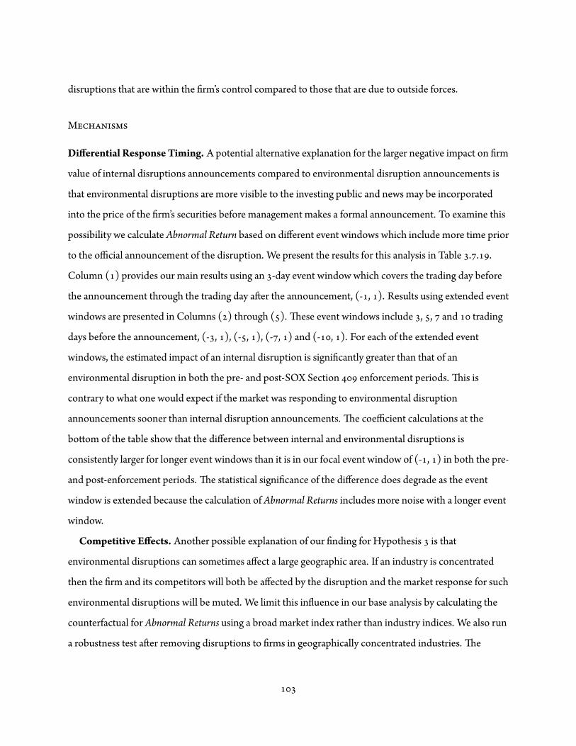
disruptions that are within the rm’s control compared to those that are due to outside forces.

M

Differential Response Timing. A potential alternative explanation for the larger negative impact on rm

value of internal disruptions announcements compared to environmental disruption announcements is

that environmental disruptions are more visible to the investing public and news may be incorporated

into the price of the rm’s securities before management makes a formal announcement. To examine this

possibility we calculate Abnormal Return based on different event windows which include more time prior

to the official announcement of the disruption. We present the results for this analysis in Table . . .

Column ( ) provides our main results using an -day event window which covers the trading day before

the announcement through the trading day a er the announcement, (- , ). Results using extended event

windows are presented in Columns ( ) through ( ). ese event windows include , , and trading

days before the announcement, (- , ), (- , ), (- , ) and (- , ). For each of the extended event

windows, the estimated impact of an internal disruption is signi cantly greater than that of an

environmental disruption in both the pre- and post-SOX Section enforcement periods. is is

contrary to what one would expect if the market was responding to environmental disruption

announcements sooner than internal disruption announcements. e coefficient calculations at the

bo om of the table show that the difference between internal and environmental disruptions is

consistently larger for longer event windows than it is in our focal event window of (- , ) in both the pre-

and post-enforcement periods. e statistical signi cance of the difference does degrade as the event

window is extended because the calculation of Abnormal Returns includes more noise with a longer event

window.

Competitive Effects. Another possible explanation of our nding for Hypothesis is that

environmental disruptions can sometimes affect a large geographic area. If an industry is concentrated

then the rm and its competitors will both be affected by the disruption and the market response for such

environmental disruptions will be muted. We limit this in uence in our base analysis by calculating the

counterfactual for Abnormal Returns using a broad market index rather than industry indices. We also run

a robustness test a er removing disruptions to rms in geographically concentrated industries. e

industries that we exclude are electronics (SIC - ), automotive (SIC - ), and aerospace

(SIC - ). e results are presented in Column ( ) of Table . . and continue to provide

support for Hypothesis .

Differential Earnings Impact. We guard against the possibility that disruptions may impact the rm’s

market value differently because they are simply lower magnitude or have a smaller direct effect on the

rm’s earnings. For instance, environmental disruptions in general could have a lower impact on rm

value because rms may be more likely to suffer insurable losses from such disruptions. In all of our tests

on Abnormal Returnswe account for the possibility of a differential earnings impact by including the

Earnings Surprise control in our speci cations.

R T

We run the same ba ery of robustness tests that we describe in . . , including using alternative sample

windows, alternative calculations of Abnormal Return, winsorizing outlying independent variables, and

controlling for multiple disruptions by individual rms (not presented). e main inferences from our

analysis continue to hold under these robustness tests.

. L E

e questions we seek to answer are potentially susceptible to endogeneity issues. Indeed, it is this

possibility for endogeneity that has been least explored in the existing literature on this topic, and our

effort to address it marks an important component of our ndings. To that end, we have identi ed a

natural experiment (the change in disclosure regulations) that helps us to address some of the potential

endogeneity that all research on this topic is susceptible to, namely the propensity of some rms to hide

emerging disruptions. Our research makes a valuable contribution by addressing these unexplored

associations.

As with other large-sample empirical studies of disruptions we cite, our analysis is hampered by

incomplete information about the economic magnitude of disruptions; few disruption announcements

disclose such information consistently. We make and important step in addressing this de ciency by

including the Earnings Surprise control variable, but a data source that more consistently reports on the

magnitude of disruptions would be helpful and might generate additional insights.

Another limitation to our study is that we cannot eliminate the possibility that other unmeasured

contemporaneous forces are driving the increase in disruption announcements and the market’s response.

In addition to the robustness tests identi ed above, we sought to validate our results by interviewing

current and former executives of publicly traded rms about their disclosure practices pertaining to

operational disruptions. e feedback we received aligns with our theory that managers did, in fact,

refrain from disclosing material disruptions if they could “manage it within the quarter.” For instance, the

President of a large supermarket chain acknowledged “[we] would really weigh the pros and cons [of

making an announcement], since you don’t want to prematurely spook the market.” e CEO and

Chairman of a major electronics distributor made the same point more colorfully: “Firms will be hesitant

to pull their pants down in public unless they are forced to do it.” e interviews support the view that,

prior to Section enforcement, managers avoided announcing disruptions generally, but felt

compelled to announce those that were so large as to make them difficult to address privately. e

increased formalization of disclosure practices as a result of SOX regulations curtailed this practice.

Post-enforcement announcements, by contrast, include disruptions material enough to warrant

disclosure but that might not have otherwise been announced had management retained more discretion.

. D M I

We estimate the rms twice as likely to disclose supply chain disruption announcements following the

enforcement date of SOX Section . e average impact of a disruption on the rm’s share price is

reduced from - . percentage points to - . a er the enforcement of Section of SOX. We provide

considerable evidence that managers exercised consideration discretion in reporting material disruptions

and that Section enforcement tempered their predisposition to underreport disruptions that are less

damaging but still consequential to the rm’s operations under the SOX guidelines.

We also show that the impact of a disruption on rm value depends heavily on whether or not the

disruption is a ributed to factors under the rm’s control in both the pre- and post-Section

enforcement period. In the pre-Section period, the average impact on the rm’s stock price is - .

percentage points for an internal disruption and - . percentage points for disruptions a ributed to the

environment. ese values drop to - . percentage points and - . percentage points in the post-Section

period. Given that the median daily return was - . percentage points for the observations in our

database that did not involve a disruption, the results from our analysis are economically signi cant.

We draw two insights from these results. First, disruptions that are under the rm’s control are much

more damaging to rm value than those not under the rm’s control, even a er accounting for their

impact on current earnings. While this difference persists in both the pre- and post-enforcement period, it

is reduced in the post-enforcement period. Second, and relatedly, the enforcement of Section

reduced the impact of internal disruptions on the rm’s stock price more than that of environmental

disruptions. is difference persists (and actually becomes more pronounced) a er accounting for the

possibility that the stock market responds to environmental disruptions before the rm officially

announces them. is difference can reasonably be explained by management’s ability to avoid revealing

internal disruptions compared to environmental disruptions since the la er are more likely to be

observable by external parties.

e impact of disruptions on rm value can vary widely, but there are clearly instances when

disruptions have a devastating effect. We have shown that the type of disruption ma ers in identifying the

magnitude of a disruption’s impact on a rm’s share price. Disruptions a ributed to factors within the rm

or its supply chain are far more damaging than disruptions a ributed to factors in the environment. It is

important for managers and investors alike to recognize the types of disruptions and the rm

characteristics that contribute disproportionately to more undesirable outcomes. Countermeasures to

mitigate the risk of disruptions have a cost, and insights into the types of disruptions that represent the

greatest risk to company value will help managers assess whether the company is investing appropriately

to mitigate the most material risks.

Table . . : Sample summary

Disruptions Earnings-OnlyYear Frequency Percent Frequency Percent

.. .. .. .. .. .. .. .. .. .. .. .. .. .. .

Total

Disruptions Earnings-OnlyCurrent Quarter Sales Frequency Percent Frequency Percent

Current Quarter Sales< M . .Sales≥ M and< M . .Sales≥ M and< M . .Sales≥ M . .Sales unknown . .Total

Table . . : Description of Form 8-K Items

ItemDescription StatusSection - Registrant Business andOperationsItem . Entry into a Material De nitive Agreement NewItem . Termination of a Material De nitive Agreement NewItem . Bankruptcy or Receivership UnchangedSection - Financial InformationItem . Completion of Acquisition or Disposition of Assets Largely UnchangedItem . Results of Operations and Financial Condition UnchangedItem . Creation of a Direct or Off-Balance Sheet Obligation NewItem . Events at Accelerate or Increase a Direct or Off-Balance Sheet Obligation NewItem . Costs Associated with Exit or Disposal Activities NewItem . Material Impairments NewSection - Securities and TradingMarketsItem . Notice of Delisting or Transfer of Listing NewItem . Unregistered Sales of Equity Securities Previously on Q/KItem . Material Modi cations to Rights of Security Holders Previously on Q/KSection -Ma ers Related to Accountants and Financial StatementsItem . Changes in Registrant’s Certifying Accountant UnchangedItem . Non-Reliance on Previously Issued Financial Statements NewSection - Corporate Governance andManagementItem . Changes in Control of Registrant Largely UnchangedItem . Departure, Election or Appointment of Directors or Principal Officers ExpandedItem . Amendments to Articles of Incorporation or Bylaws; Change in Fiscal Year ExpandedItem . Suspension of Trading Under Registrant’s Employee Bene t Plans ExpandedItem . Amendments to or Waiver of the Registrant’s Code of Ethics UnchangedSection - Regulation FDItem . Regulation FD Disclosure UnchangedSection - Other EventsItem . Other Events Unchanged

continued on the next page

Table . . – continued from previous pageItemDescription Status

Section - Financial Statements and ExhibitsItem . Financial Statements and Exhibits Largely UnchangedNote :Table developed based on information contained in the SEC nal ruling, “Additional Form -K Disclosure Requirements and Acceleration of FilingDate (Final Rule)”, Federal Register. : - .

Table . . : Description of Variables Used in the Analysis of the Likelihood of a Disruption Announcement

Variable DescriptionAnnounced Disruption Supply chain disruption was announced by the rmAnnounced Internal Disruption a ributed to factors internal to the rm’s operations was announced by the rmAnnounced External Disruption a ributed to factors external to the rm but within its supply chain was announced by the rmAnnounced Environment Disruption a ributed to factors in the environment was announced by the rmPost-SOX Quarter Period is before the enforcement quarter of the SOX SectionAccelerated Filer Indicator identifying whether the rm has accelerated ling status in the quarter of the announcementEarnings Surprise e difference between the earnings per share provided in the announcement and the average of the analysts’ forecast.Debt-to-Equity Ratio e book value of the rm’s long-term debt divided by market value of its common equity, lagged one quarterMarket-to-Book Ratio e market value of the rm’s common equity divided by the book value of its common equity, lagged one quarterFixed Assets Ratio e ratio of property, plant, and equipment divided by total assets, lagged one quarterLog Sales e natural log of quarterly sales (in M), lagged one quarter

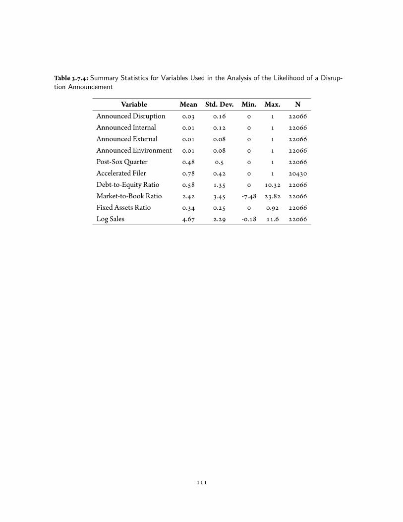
Table . . : Summary Statistics for Variables Used in the Analysis of the Likelihood of a Disrup-tion Announcement

Variable Mean Std. Dev. Min. Max. NAnnounced Disruption . .Announced Internal . .Announced External . .Announced Environment . .Post-Sox Quarter . .Accelerated Filer . .Debt-to-Equity Ratio . . .Market-to-Book Ratio . . - . .Fixed Assets Ratio . . .Log Sales . . - . .

Table . . : Correlations for Variables Used in the Analysis of the Likelihood of a Disruption Announcement

Variables Anno

unce

dDisr

uptio

n

Anno

unce

dIn

tern

al

Anno

unce

dEx

tern

al

Anno

unce

dEn

viro

nmen

t

Post-S

oxQ

uarter

Acce

leratedFi

ler

Deb

t-to-

Equity

Ratio

Marke

t-to-

Book

Ratio

Fixe

dAssetsR

atio

LogSa

les

Announced Disruption .Announced Internal . .Announced External . . .Announced Environment . . . .Post-Sox Quarter . . . . .Accelerated Filer . . . . . .Debt-to-Equity Ratio - . - . - . - . - . - . .Market-to-Book Ratio . . . . - . . - . .Fixed Assets Ratio . . - . . - . . . - . .Log Sales . . - . . . . . - . . .

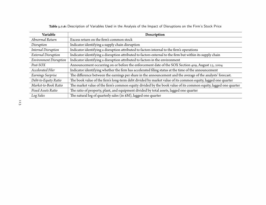
Table . . : Description of Variables Used in the Analysis of the Impact of Disruptions on the Firm’s Stock Price

Variable DescriptionAbnormal Return Excess return on the rm’s common stockDisruption Indicator identifying a supply chain disruptionInternal Disruption Indicator identifying a disruption a ributed to factors internal to the rm’s operationsExternal Disruption Indicator identifying a disruption a ributed to factors external to the rm but within its supply chainEnvironment Disruption Indicator identifying a disruption a ributed to factors in the environmentPost-SOX Announcement occurring on or before the enforcement date of the SOX Section , August ,Accelerated Filer Indicator identifying whether the rm has accelerated ling status at the time of the announcementEarnings Surprise e difference between the earnings per share in the announcement and the average of the analysts’ forecast.Debt-to-Equity Ratio e book value of the rm’s long-term debt divided by market value of its common equity, lagged one quarterMarket-to-Book Ratio e market value of the rm’s common equity divided by the book value of its common equity, lagged one quarterFixed Assets Ratio e ratio of property, plant, and equipment divided by total assets, lagged one quarterLog Sales e natural log of quarterly sales (in M), lagged one quarter

Table . . : Summary Statistics for Variables Used in the Analysis of the Impact of Disruptions onthe Firm’s Stock Price

Variable Mean Std. Dev. Min. Max. NAbnormal Return - . . - . .Disruption . .Internal Disruption . .External Disruption . .Environment Disruption . .Post-Sox . .Accelerated Filer . .Earnings Surprise . - . .Debt-to-Equity Ratio . . .Market-to-Book Ratio . . - . .Fixed Assets Ratio . . .Log Sales . . .

Table . . : Correlations for Variables Used in the Analysis of the Impact of Disruptions on the Firm’s Stock Price

Variables Abno

rmal

Retur

n

Disr

uptio

n

Intern

alDisr

uptio

n

Extern

alDisr

uptio

n

Enviro

nmen

tDisr

uptio

n

Post-S

ox

Acce

leratedFi

ler

Earn

ings

Surp

rise

Deb

t-to-

Equity

Ratio

Marke

t-to-

Book

Ratio

Fixe

dAssetsR

atio

LogSa

les

Abnormal Return .Disruption - . .Internal Disruption - . . .External Disruption - . . - . .Environment Disruption - . . - . . .Post-Sox . . - . - . . .Accelerated Filer - . - . - . - . - . . .Earnings Surprise . . . . . . . .Debt-to-Equity Ratio . - . . - . - . - . - . - . .Market-to-Book Ratio - . - . - . . . . . . - . .Fixed Assets Ratio . - . - . - . . . . . . - . .Log Sales . - . - . - . . . . . . . . .

Table . . : Estimating the likelihood of a disruption announcement.

Dependent Variable: Announced DisruptionCoefficient Odds Ratio

( ) ( )

Post-SOX Quarter . ** . **[ . ] [ . ]

Debt-to-Equity Ratio - . ** . **[ . ] [ . ]

Market-to-Book Ratio . * . *[ . ] [ . ]

Fixed Assets Ratio . .[ . ] [ . ]

Log Sales . .[ . ] [ . ]

Observations , ,Number of FirmsNumber of DisruptionsPseudo R . .Mean, pre- . .Mean, post- . .Notes: Conditional xed effects logistic estimation. Robust standard errors clustered by rm in brackets.

** p< . , * p< . , + p< .

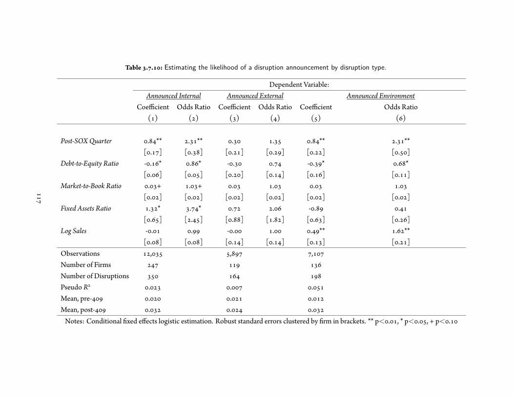
Table . . : Estimating the likelihood of a disruption announcement by disruption type.

Dependent Variable:Announced Internal Announced External Announced Environment

Coefficient Odds Ratio Coefficient Odds Ratio Coefficient Odds Ratio( ) ( ) ( ) ( ) ( ) ( )

Post-SOX Quarter . ** . ** . . . ** . **[ . ] [ . ] [ . ] [ . ] [ . ] [ . ]

Debt-to-Equity Ratio - . * . * - . . - . * . *[ . ] [ . ] [ . ] [ . ] [ . ] [ . ]

Market-to-Book Ratio . + . + . . . .[ . ] [ . ] [ . ] [ . ] [ . ] [ . ]

Fixed Assets Ratio . * . * . . - . .[ . ] [ . ] [ . ] [ . ] [ . ] [ . ]

Log Sales - . . - . . . ** . **[ . ] [ . ] [ . ] [ . ] [ . ] [ . ]

Observations , , ,Number of FirmsNumber of DisruptionsPseudo R . . .Mean, pre- . . .Mean, post- . . .Notes: Conditional xed effects logistic estimation. Robust standard errors clustered by rm in brackets. ** p< . , * p< . , + p< .

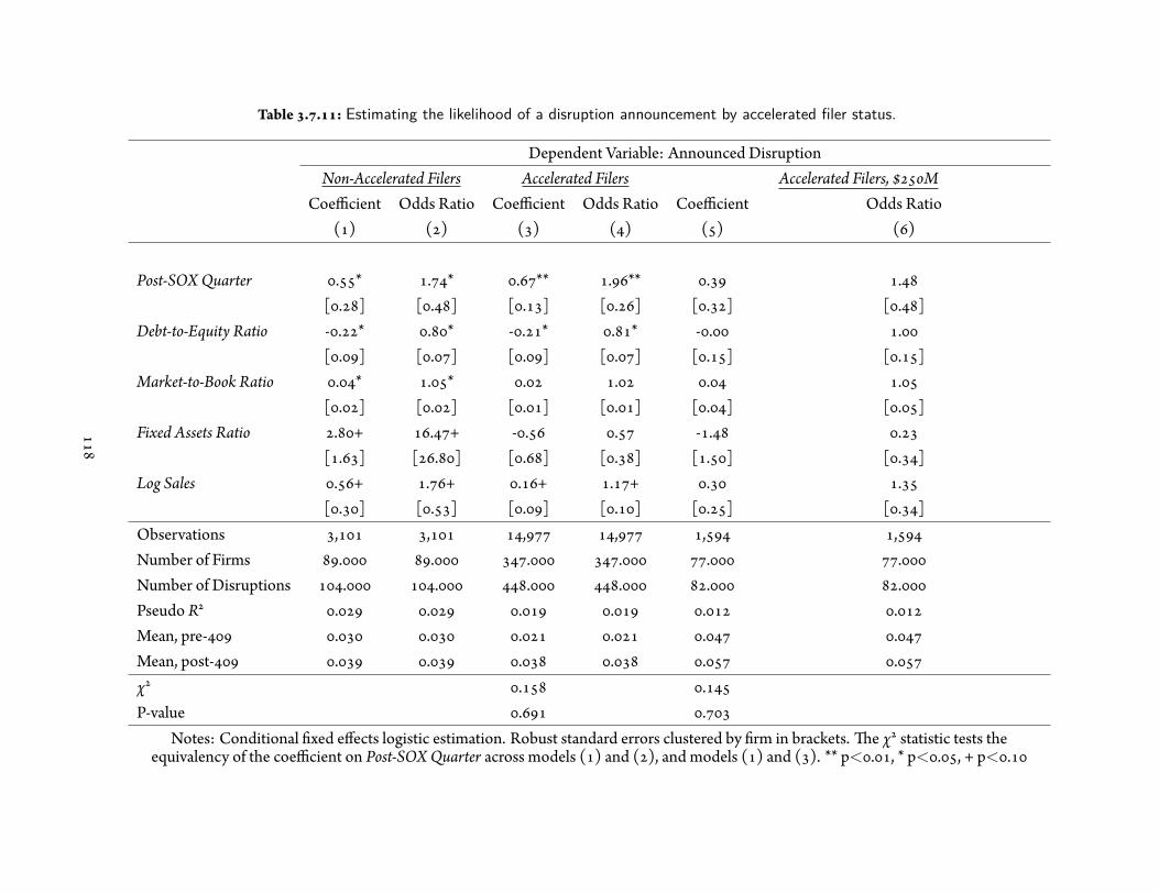
Table . . : Estimating the likelihood of a disruption announcement by accelerated filer status.

Dependent Variable: Announced DisruptionNon-Accelerated Filers Accelerated Filers Accelerated Filers, M

Coefficient Odds Ratio Coefficient Odds Ratio Coefficient Odds Ratio( ) ( ) ( ) ( ) ( ) ( )

Post-SOX Quarter . * . * . ** . ** . .[ . ] [ . ] [ . ] [ . ] [ . ] [ . ]

Debt-to-Equity Ratio - . * . * - . * . * - . .[ . ] [ . ] [ . ] [ . ] [ . ] [ . ]

Market-to-Book Ratio . * . * . . . .[ . ] [ . ] [ . ] [ . ] [ . ] [ . ]

Fixed Assets Ratio . + . + - . . - . .[ . ] [ . ] [ . ] [ . ] [ . ] [ . ]

Log Sales . + . + . + . + . .[ . ] [ . ] [ . ] [ . ] [ . ] [ . ]

Observations , , , , , ,Number of Firms . . . . . .Number of Disruptions . . . . . .Pseudo R . . . . . .Mean, pre- . . . . . .Mean, post- . . . . . .χ . .P-value . .

Notes: Conditional xed effects logistic estimation. Robust standard errors clustered by rm in brackets. e χ statistic tests theequivalency of the coefficient on Post-SOX Quarter across models ( ) and ( ), and models ( ) and ( ). ** p< . , * p< . , + p< .

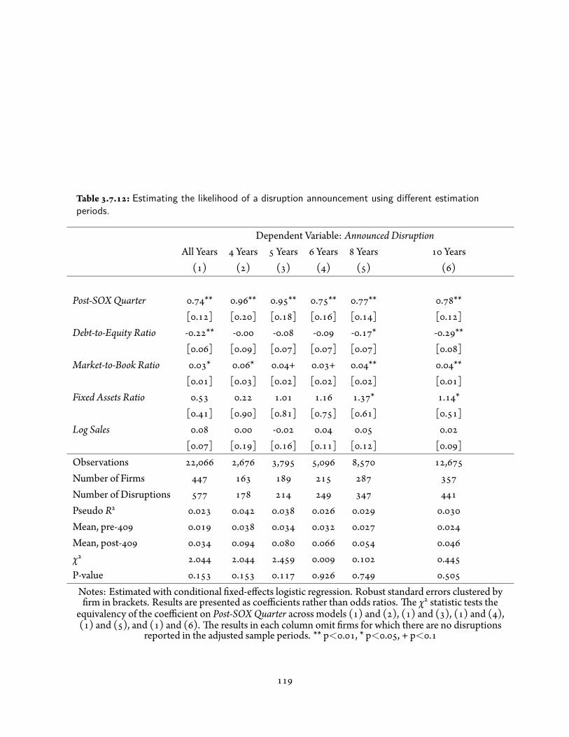
Table . . : Estimating the likelihood of a disruption announcement using different estimationperiods.

Dependent Variable: Announced DisruptionAll Years Years Years Years Years Years

( ) ( ) ( ) ( ) ( ) ( )

Post-SOX Quarter . ** . ** . ** . ** . ** . **[ . ] [ . ] [ . ] [ . ] [ . ] [ . ]

Debt-to-Equity Ratio - . ** - . - . - . - . * - . **[ . ] [ . ] [ . ] [ . ] [ . ] [ . ]

Market-to-Book Ratio . * . * . + . + . ** . **[ . ] [ . ] [ . ] [ . ] [ . ] [ . ]

Fixed Assets Ratio . . . . . * . *[ . ] [ . ] [ . ] [ . ] [ . ] [ . ]

Log Sales . . - . . . .[ . ] [ . ] [ . ] [ . ] [ . ] [ . ]

Observations , , , , , ,Number of FirmsNumber of DisruptionsPseudo R . . . . . .Mean, pre- . . . . . .Mean, post- . . . . . .χ . . . . . .P-value . . . . . .Notes: Estimated with conditional xed-effects logistic regression. Robust standard errors clustered by

rm in brackets. Results are presented as coefficients rather than odds ratios. e χ statistic tests theequivalency of the coefficient on Post-SOX Quarter across models ( ) and ( ), ( ) and ( ), ( ) and ( ),( ) and ( ), and ( ) and ( ). e results in each column omit rms for which there are no disruptions

reported in the adjusted sample periods. ** p< . , * p< . , + p< .

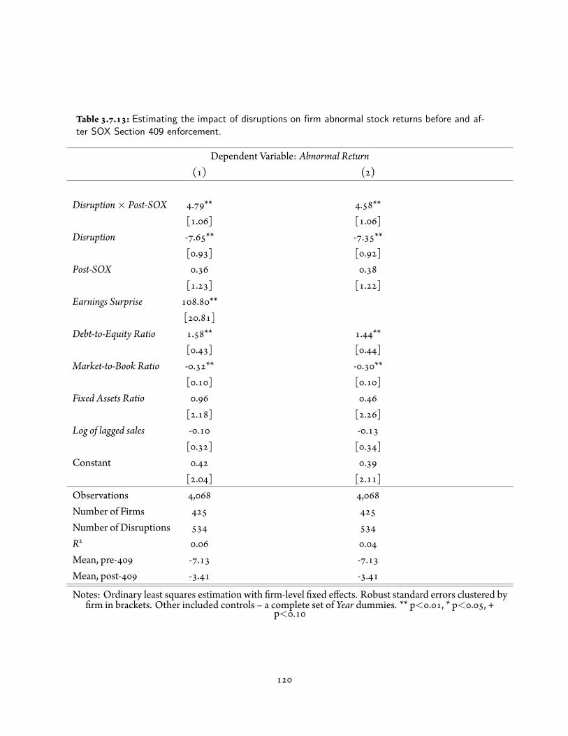
Table . . : Estimating the impact of disruptions on firm abnormal stock returns before and af-ter SOX Section 409 enforcement.

Dependent Variable: Abnormal Return( ) ( )

Disruption× Post-SOX . ** . **[ . ] [ . ]

Disruption - . ** - . **[ . ] [ . ]

Post-SOX . .[ . ] [ . ]

Earnings Surprise . **[ . ]

Debt-to-Equity Ratio . ** . **[ . ] [ . ]

Market-to-Book Ratio - . ** - . **[ . ] [ . ]

Fixed Assets Ratio . .[ . ] [ . ]

Log of lagged sales - . - .[ . ] [ . ]

Constant . .[ . ] [ . ]

Observations , ,Number of FirmsNumber of DisruptionsR . .Mean, pre- - . - .Mean, post- - . - .

Notes: Ordinary least squares estimation with rm-level xed effects. Robust standard errors clustered byrm in brackets. Other included controls – a complete set of Year dummies. ** p< . , * p< . , +

p< .

Table . . : Estimating the impact on stock returns of announced disruptions by accelerated filerstatus.

Dependent Variable: Abnormal Return( ) ( )

(A) Disruption× Post-SOX . ** . *[ . ] [ . ]

(B) Disruption× Post-SOX × Accelerated Filer - . - .[ . ] [ . ]

Disruption - . ** - . **[ . ] [ . ]

Post-SOX . .[ . ] [ . ]

Accelerated Filer - . ** - . +[ . ] [ . ]

Disruption× Accelerated Filer . .[ . ] [ . ]

Post-SOX × Accelerated Filer - . - . +[ . ] [ . ]

Constant . .[ . ] [ . ]

Observations , ,Number of FirmsNumber of DisruptionsNumber AF DisruptionsNumber NAF DisruptionsR . .Mean, pre- - . - .Mean, post- - . - .Coeff on (A)+(B) . .Wald: (A)+(B)= ? . ** .

Notes: Ordinary least squares estimation with rm-level xed effects. Robust standard errors clustered byrm in brackets. Model ( ) includes all observations. Model( ) includes only observations with a public

oat≤ M. Included controls – Earnings Surprise, Fixed Asset Ratio,Market-to-Book Ratio,Debt-to-Equity Ratio, Log Sales, and a complete set of year dummies, Year. Wald tests report F statistics. **

p< . , * p< . , + p< .

Table . . : Estimating the impact on stock returns of announced disruptions after includingmore pre-announcement days in the calculation of Abnormal Returns.

Dependent Variable: Abnormal ReturnW(- , ) W(- , ) W(- , ) W(- , )

( ) ( ) ( ) ( )

Disruption - . ** - . ** - . ** - . **[ . ] [ . ] [ . ] [ . ]

Disruption× Post-SOX . ** . ** . ** . **[ . ] [ . ] [ . ] [ . ]

Post-SOX . - . - . - .[ . ] [ . ] [ . ] [ . ]

Constant . . . .[ . ] [ . ] [ . ] [ . ]

Observations , , , ,Number of FirmsNumber of DisruptionsR . . . .Mean, pre- - . - . - . - .Mean, post- - . - . - . - .χ , pre- . . .P-value, pre- . . .χ , post- . . .P-value, post- . . .Notes: Ordinary least squares estimation with rm-level xed effects. Robust standard errors clustered by

rm in brackets. e Abnormal Return dependent variable in column ( ) uses a (- , ) event window,column ( ) uses a (- , ) event window, column ( ) uses a (- , ) event window, and column ( ) uses a(- , ) event window. Included controls – Earnings Surprise, Fixed Asset Ratio,Market-to-Book Ratio,

Debt-to-Equity Ratio, Log Sales, and a complete set of year dummies, Year. e pre- χ statistic tests theequivalency of the coefficient onDisruption across models ( ) and ( ), ( ) and ( ), and ( ) and ( ). e

post- χ statistic tests the equivalency of the coefficient onDisruption + Disruption×Post-SOX. **p< . , * p< . , + p< .

Table . . : Estimating the impact on stock returns of announced disruptions using differentestimation periods.

Dependent Variable: Abnormal ReturnAllYears Years Years Years Years Years

( ) ( ) ( ) ( ) ( ) ( )

Disruption - . ** - . ** - . ** - . ** - . ** - . **[ . ] [ . ] [ . ] [ . ] [ . ] [ . ]

Disruption× Post-SOX . ** . ** . ** . * . + .[ . ] [ . ] [ . ] [ . ] [ . ] [ . ]

Post-SOX . . . . . .[ . ] [ . ] [ . ] [ . ] [ . ] [ . ]

Constant . . . . . + .[ . ] [ . ] [ . ] [ . ] [ . ] [ . ]

Observations , , , , , ,R . . . . . .Number of FirmsNumber of DisruptionsMean, pre- - . - . - . - . - . - .Mean, post- - . - . - . - . - . - .χ , pre- . . . . .P-value, pre- . . . . .χ , post- . . . . .P-value, post- . . . . .Notes: Ordinary least squares estimation with rm-level xed effects. Robust standard errors clustered by

rm in brackets. Included controls – Earnings Surprise, Fixed Asset Ratio,Market-to-Book Ratio,Debt-to-Equity Ratio, Log Sales, and a complete set of year dummies, Year. Wald tests report F statistics.

e pre- χ statistic tests the equivalency of the coefficient onDisruption across models ( ) and ( ),( ) and ( ), ( ) and ( ), ( ) and ( ), and ( ) and ( ). e post- χ statistic tests the equivalency of

the coefficient onDisruption + Disruption×Post-SOX. ** p< . , * p< . , + p< .

Table . . : Estimating the impact on stock returns of announced disruptions after expandingthe event window in the calculation of Abnormal Returns.

Dependent Variable: Abnormal ReturnW(- , ) W(- , ) W(- , ) W(- , ) W(- , )

( ) ( ) ( ) ( ) ( )

Disruption - . ** - . ** - . ** - . ** - . **[ . ] [ . ] [ . ] [ . ] [ . ]

Disruption× Post-SOX . ** . ** . ** . ** . **[ . ] [ . ] [ . ] [ . ] [ . ]

Post-SOX . - . - . - . - .[ . ] [ . ] [ . ] [ . ] [ . ]

Constant . . . . .[ . ] [ . ] [ . ] [ . ] [ . ]

Observations , , , , ,R . . . . .Number of FirmsNumber of DisruptionsMean, pre- - . - . - . - . - .Mean, post- - . - . - . - . - .Notes: Ordinary least squares estimation with rm-level xed effects. Robust standard errors clustered by

rm in brackets. e Abnormal Return dependent variable in column ( ) uses a (- , ) event window,column ( ) uses a (- , ), column ( ) uses a (- , ), column ( ) uses a (- , ), and column ( ) uses a(- , ). Included controls – Earnings Surprise, Fixed Asset Ratio,Market-to-Book Ratio,Debt-to-EquityRatio, Log Sales, and a complete set of year dummies, Year. Wald tests report F statistics. ** p< . , *

p< . , + p< .

Table . . : Estimating the impact of different types of disruptions on firm abnormal stock re-turns before and after SOX Section 409 enforcement.

Dependent Variable: Abnormal Return( ) ( )

(A) Internal Disruption× Post-SOX . ** . **[ . ] [ . ]

External Disruption× Post-SOX . * . *[ . ] [ . ]

(B) Environment Disruption× Post-SOX . .[ . ] [ . ]

(C) Internal Disruption - . ** - . **[ . ] [ . ]

External Disruption - . ** - . **[ . ] [ . ]

(D) Environment Disruption - . - .[ . ] [ . ]

Post-SOX . .[ . ] [ . ]

Constant . .[ . ] [ . ]

Observations , ,Number of FirmsNumber of DisruptionsR . .Mean, pre- - . - .Mean, post- - . - .Wald: (C)-(D)= ? . ** . **Wald: (A)+(C)-(B)-(D)= ? . ** . *

Notes: Ordinary least squares estimation with rm-level xed effects. Robust standard errors clustered byrm in brackets. Earnings Surprise, Fixed Asset Ratio,Market-to-Book Ratio,Debt-to-Equity Ratio, Log Sales,and a complete set of year dummies, Year. Wald tests report F statistics. ** p< . , * p< . , + p< .

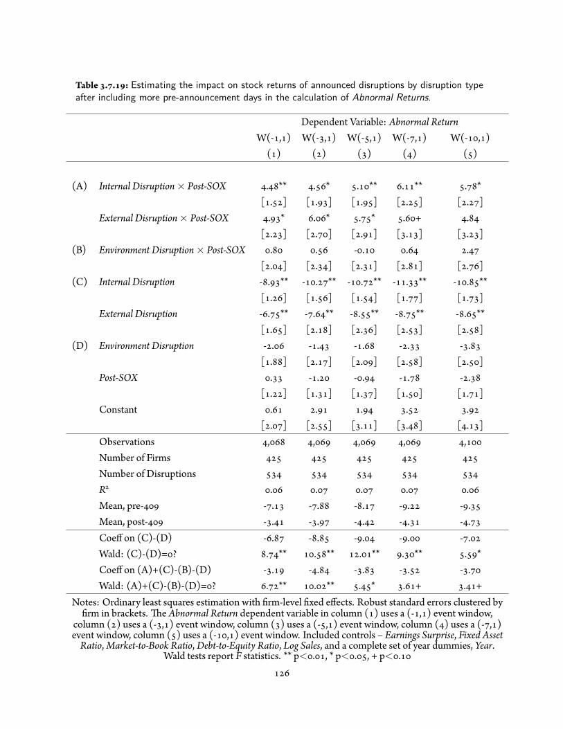
Table . . : Estimating the impact on stock returns of announced disruptions by disruption typeafter including more pre-announcement days in the calculation of Abnormal Returns.

Dependent Variable: Abnormal ReturnW(- , ) W(- , ) W(- , ) W(- , ) W(- , )

( ) ( ) ( ) ( ) ( )

(A) Internal Disruption× Post-SOX . ** . * . ** . ** . *[ . ] [ . ] [ . ] [ . ] [ . ]

External Disruption× Post-SOX . * . * . * . + .[ . ] [ . ] [ . ] [ . ] [ . ]

(B) Environment Disruption× Post-SOX . . - . . .[ . ] [ . ] [ . ] [ . ] [ . ]

(C) Internal Disruption - . ** - . ** - . ** - . ** - . **[ . ] [ . ] [ . ] [ . ] [ . ]

External Disruption - . ** - . ** - . ** - . ** - . **[ . ] [ . ] [ . ] [ . ] [ . ]

(D) Environment Disruption - . - . - . - . - .[ . ] [ . ] [ . ] [ . ] [ . ]

Post-SOX . - . - . - . - .[ . ] [ . ] [ . ] [ . ] [ . ]

Constant . . . . .[ . ] [ . ] [ . ] [ . ] [ . ]

Observations , , , , ,Number of FirmsNumber of DisruptionsR . . . . .Mean, pre- - . - . - . - . - .Mean, post- - . - . - . - . - .Coeff on (C)-(D) - . - . - . - . - .Wald: (C)-(D)= ? . ** . ** . ** . ** . *Coeff on (A)+(C)-(B)-(D) - . - . - . - . - .Wald: (A)+(C)-(B)-(D)= ? . ** . ** . * . + . +

Notes: Ordinary least squares estimation with rm-level xed effects. Robust standard errors clustered byrm in brackets. e Abnormal Return dependent variable in column ( ) uses a (- , ) event window,

column ( ) uses a (- , ) event window, column ( ) uses a (- , ) event window, column ( ) uses a (- , )event window, column ( ) uses a (- , ) event window. Included controls – Earnings Surprise, Fixed AssetRatio,Market-to-Book Ratio,Debt-to-Equity Ratio, Log Sales, and a complete set of year dummies, Year.

Wald tests report F statistics. ** p< . , * p< . , + p< .

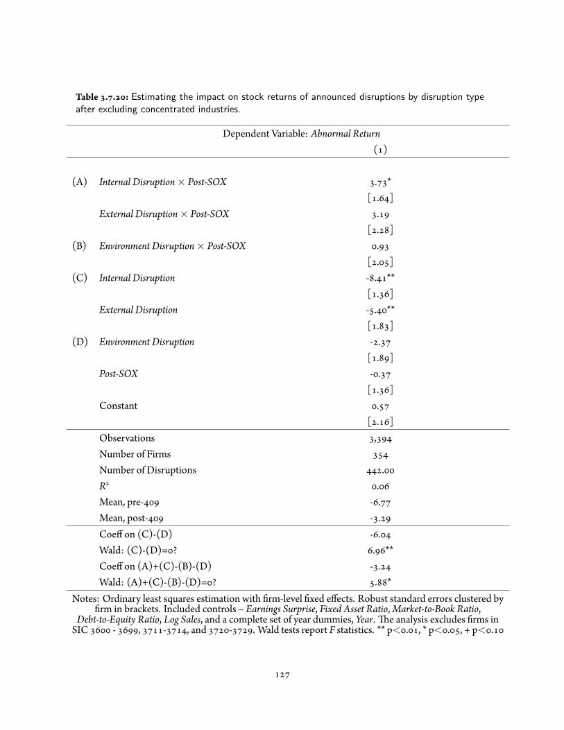
Table . . : Estimating the impact on stock returns of announced disruptions by disruption typeafter excluding concentrated industries.

Dependent Variable: Abnormal Return( )

(A) Internal Disruption× Post-SOX . *[ . ]

External Disruption× Post-SOX .[ . ]

(B) Environment Disruption× Post-SOX .[ . ]

(C) Internal Disruption - . **[ . ]

External Disruption - . **[ . ]

(D) Environment Disruption - .[ . ]

Post-SOX - .[ . ]

Constant .[ . ]

Observations ,Number of FirmsNumber of Disruptions .R .Mean, pre- - .Mean, post- - .Coeff on (C)-(D) - .Wald: (C)-(D)= ? . **Coeff on (A)+(C)-(B)-(D) - .Wald: (A)+(C)-(B)-(D)= ? . *

Notes: Ordinary least squares estimation with rm-level xed effects. Robust standard errors clustered byrm in brackets. Included controls – Earnings Surprise, Fixed Asset Ratio,Market-to-Book Ratio,

Debt-to-Equity Ratio, Log Sales, and a complete set of year dummies, Year. e analysis excludes rms inSIC - , - , and - . Wald tests report F statistics. ** p< . , * p< . , + p< .

References

th Congress. Sarbanes-oxley act of , . U.S. Government Printing Office, USC , – .Philippe Aghion and Patrick Bolton. Contracts as a barrier to entry. e American Economic Review, ( ):

– , .Krishnan S. Anand and Manu Goyal. Strategic information management under leakage in a supply chain.

Management Science, ( ): – , .Jeffrey Banks, Colin Camerer, and David Porter. An experimental analysis of Nash re nements in signaling

games. Games and Economic Behavior, ( ): – , .Dominic Barton. Capitalism for the long term. Harvard Business Review, March : – , .Lucian Arye Bebchuk and Lars A. Stole. Do short-term objectives lead to under- or overinvestment in long-term

projects? e Journal of Finance, ( ): – , .Adolf Augustus Berle and Gardiner Coit Means. e modern corporation and private property. Macmillan, New

York, .Gary E. Bolton and Elena Katok. Learning by doing in the newsvendor problem: A laboratory investigation of the

role of experience and feedback. Manufacturing and Service Operations Management, ( ): – , .Patrick Bolton and M. Dewatripont. Contract theory. MIT Press, Cambridge, Mass., .A.J. Bostian, Charles A. Holt, and Angela M. Smith. Newsvendor “pull-to-center” effect: Adaptive learning in a

laboratory experiment. Manufacturing and Service Operations Management, ( ): – , .Jordi Brandts and Charles A. Holt. An experimental test of equilibrium dominance in signaling games. e

American Economic Review, ( ): – , .Michael J. Braunscheidel and Nallan C. Suresh. e organizational antecedents of a rm’s supply chain agility for

risk mitigation and response. Journal of Operations Management, ( ): – , .Richard A. Brealey, Stewart C. Myers, and Franklin Allen. Principles of corporate nance. McGraw-Hill/Irwin,

New York, th edition, .William Brown and Frank Nasuti. What ERP systems can tell us about Sarbanes-Oxley. Information Management

and Computer Security, ( ): – , a.William Brown and Frank Nasuti. Sarbanes–Oxley and enterprise security: IT governance and what it takes to

get the job done. EDPACS, ( ): – , b.Jr. Bruns, William J. and Kenneth A. Merchant. e dangerous morality of managing earnings. Management

Accounting, ( ): – , .Brian J. Bushee. e in uence of institutional investors on myopic R&D investment behavior. e Accounting

Review, ( ): – , .Ellen Byron. Clarins puts on its best face in U.S., . Wall Street Journal; March , ; Dow Jones, Inc.

Gérard P. Cachon and Martin A. Lariviere. Contracting to assure supply: How to share demand forecasts in asupply chain. Management Science, ( ): – , .

Mark M. Carhart. On persistence in mutual fund performance. e Journal of Finance, ( ): – , .Kam C. Chan, Barbara Farrell, and Lee Picheng. Earnings management of rms reporting material internal

control weaknesses under Section of the Sarbanes-Oxley Act. Auditing, ( ): – , .In-Koo Cho and David M. Kreps. Signaling games and stable equilibria. e Quarterly Journal of Economics,

( ): – , .Jiri Chod, Nils Rudi, and Jan A. Van Mieghem. Operational exibility and nancial hedging: Complements or

substitutes? Management Science, ( ): – , .Sunil Chopra and Peter Meindl. Supply Chain Management: Strategy Planning and Operation, volume . Prentice

Hall, Upper Saddle River, N.J., .Martin Christopher and Hau Lee. Mitigating supply chain risk through improved con dence. International

Journal of Physical Distribution and Logistics Management, ( ): – , .John C. Coates. e goals and promise of the Sarbanes-Oxley Act. e Journal of Economic Perspectives, ( ):

– , .Jr. Coffee, John C. Market failure and the economic case for a mandatory disclosure system. Virginia Law Review,

( ): – , .Daniel A. Cohen and Paul Zarowin. Accrual-based and real earnings management activities around seasoned

equity offerings. Journal of Accounting and Economics, ( ): – , .David J. Cooper and John H. Kagel. Are two heads be er than one? Team versus individual play in signaling

games. e American Economic Review, ( ): – , .Christopher W. Craighead, Jennifer Blackhurst, M. Johnny Rungtusanatham, and Robert B. Hand eld. e

severity of supply chain disruptions: Design characteristics and mitigation capabilities. Decision Sciences,( ): – , .

Laurens Debo and Senthil Veeraraghavan. Prices and congestion as signals of quality. Working paper, ChicagoBooth School of Business, University of Chicago, .

Preyas S. Desai and Kannan Srinivasan. Demand signalling under unobservable effort in franchising: Linear andnonlinear price contracts. Management Science, ( ): – , .

Vinayak Deshpande, Morris A. Cohen, and Karen Donohue. An empirical study of service differentiation forweapon system service parts. Operations Research, ( ): – , .

Frank H. Easterbrook and Daniel R. Fischel. Mandatory disclosure and the protection of investors. Virginia LawReview, ( ): – , .

Ernst&Young. Emerging trends in internal controls fourth survey and industry insights. Technical report,Ernst&Young Assurance and Advisroy Busness Services, .h p://www .eycom.ch/publications/items/sox /internalcontrol /en.pdf (accessed April , ).

Michael J Fishman and Kathleen M Hagerty. Mandatory versus voluntary disclosure in markets with informedand uninformed customers. Journal of Law, Economics, and Organization, ( ): – , .

Drew Fudenberg and Jean Tirole. Game theory. MIT Press, Cambridge, Mass., .Robert Gibbons. Game theory for applied economists. Princeton University Press, Princeton, N.J., .Frank B. Gigler and omas Hemmer. Conservatism, optimal disclosure policy, and the timeliness of nancial

reports. e Accounting Review, ( ): – , .

Armando Gomes. Going public without governance: Managerial reputation effects. e Journal of Finance,( ): – , .

John R. Graham, Campbell R. Harvey, and Shiva Rajgopal. e economic implications of corporate nancialreporting. Journal of Accounting and Economics, ( - ): – , .

Jacqueline Hammersley, Linda Myers, and Catherine Shakespeare. Market reactions to the disclosure of internalcontrol weaknesses and to the characteristics of those weaknesses under section of the Sarbanes OxleyAct of . Review of Accounting Studies, ( ): – , .

Oliver Hart. Regulation and Sarbanes-Oxley. Journal of Accounting Research, ( ): – , .Paul M. Healy and Krishna G. Palepu. Information asymmetry, corporate disclosure, and the capital markets: A

review of the empirical disclosure literature. Journal of Accounting and Economics, ( - ): – , .Kevin B. Hendricks and Vinod R. Singhal. e effect of supply chain glitches on shareholder wealth. Journal of

Operations Management, ( ): – , .Kevin B. Hendricks and Vinod R. Singhal. Association between supply chain glitches and operating

performance. Management Science, : – , a.Kevin B. Hendricks and Vinod R. Singhal. An empirical analysis of the effect of supply chain disruptions on

long-run stock price performance and equity risk of the rm. Production and Operations Management, :– , b.

Craig W. Holden and Leonard L. Lundstrum. Costly trade, managerial myopia, and long-term investment.Journal of Empirical Finance, ( ): – , .

Bengt Holmström. Managerial incentive problems: A dynamic perspective. e Review of Economic Studies,( ): – , .

Özge İşlegen and Erica L. Plambeck. Capacity leadership in supply chains with asymmetric demand informationand noncontractible capacity. Working Paper, Stanford Graduate School of Business, .

M. L. Kaarst-Brown and S. Kelly. IT governance and Sarbanes-Oxley: e latest sales pitch or real challenges forthe IT function? In Proceedings of the th Annual Hawaii International Conference on System Sciences.HICSS ’ ., pages – , .

P. R. Kleindorfer and G. H. Saad. Managing disruption risks in supply chains. Production and OperationsManagement, ( ): – , .

A. G. de Kok and Stephen C. Graves. Supply chain management: Design, coordination and operation, volume ofHandbooks in operations research and management science. Elsevier, Amsterdam; Boston, .

S. P. Kothari, S. Shu, and P. D. Wysocki. Do managers withhold bad news? Journal of Accounting Research, ( ):– , .

Mirko Kremer, Stefan Minner, and Luk N. Van Wassenhove. Do random errors explain newsvendor behavior?Manufacturing and Service Operations Management, ( ): – , .

David M. Kreps and Joel Sobel. Signalling. In Robert J. Aumann and Sergiu Hart, editors,Handbook of Gameeory with Economic Applications, volume , chapter , pages – . North-Holland; Elsevier Science

Pub. Co., Amsterdam; New York, N.Y., .Guoming Lai, Laurens Debo, and Lin Nan. Channel stuffing with short-term interest in market value.

Management Science, ( ): – , .Guoming Lai, Wenqiang Xiao, and Jun Yang. Supply chain performance under market valuation: An operational

approach to restore efficiency. Management Science, ( ): – , .

Martin A. Lariviere and V. Padmanabhan. Slo ing allowances and new product introductions. Marketing Science,( ): – , .

Jennifer B. Lawrence and Jackson W. Prentice. Empirical study: e SEC Form -K: Full disclosure or fullydiluted? Wake Forest Law Review, : – , .

Haidan Li, Morton Pincus, and Sonja Olho Rego. Market reaction to events surrounding the Sarbanes OxleyAct of and earnings management. Journal of Law and Economics, ( ): – , .

A. Craig MacKinlay. Event studies in economics and nance. Journal of Economic Literature, ( ): – , .George J. Mailath, Masahiro Okuno-Fujiwara, and Andrew Postlewaite. Belief-based re nements in signalling

games. Journal of Economic eory, ( ): – , .Andreu Mas-Colell, Michael Dennis Whinston, and Jerry R. Green. Microeconomic theory. Oxford University

Press, New York, .Ken McGee, Mark Raskino, and Brian Wood. SEC’s real-time disclosure requires four-day noti cation. Technical

report, Gartner, Inc., April , .Abagail McWilliams and Donald Siegel. Event studies in management research: eoretical and empirical issues.

e Academy of Management Journal, ( ): – , .Paul Milgrom and John Roberts. Price and advertising signals of product quality. Journal of Political Economy,

( ): – , .Steven Nahmias. Production and operations analysis. e McGraw-Hill/Irwin series. Operations and decision

sciences. McGraw-Hill/Irwin, Boston, th edition, .M. P. Narayanan. Managerial incentives for short-term results. e Journal of Finance, ( ): – , .Office of Economic Analysis. Study of the Sarbanes-Oxley Act of Section internal control over nancial

reporting requirements. Technical report, United States Securities and Exchange Commission, .h p://www.sec.gov/news/studies/ /sox- _study.pdf (accessed March , ).

Özalp Özer and Wei Wei. Strategic commitments for an optimal capacity decision under asymmetric forecastinformation. Management Science, ( ): – , .

Z. Partow and Andrew Scho er. Does game theory predict well for the wrong reasons: An experimentalinvestigation. Working papers, C.V. Starr Center for Applied Economics, New York University, .

Walter W Powell. Neither Market nor Hierarchy: Network Forms of Organizations, volume , pages – . JAIPress, Greenwich, CT, .

Alfred Rappaport. Beyond quarterly earnings, . Wall Street Journal; March , ; Dow Jones, Inc.John G. Riley. Silver signals: Twenty- ve years of screening and signaling. Journal of Economic Literature, ( ):

pp. – , .Sugata Roychowdhury. Earnings management through real activities manipulation. Journal of Accounting and

Economics, ( ): – , .Bernard Salanie. e economics of contracts : A primer. MIT Press, Cambridge, Mass., nd edition, .William Schmidt, Vishal Gaur, Richard Lai, and Ananth Raman. Signaling to partially informed investors in the

newsvendor model. Harvard Business School Working Paper - , .Maurice E. Schweitzer and Gérard P. Cachon. Decision bias in the newsvendor problem with a known demand

distribution: Experimental evidence. Management Science, ( ): – , .W. Richard Sco and Gerald F. Davis. Organizations and organizing : Rational, natural, and open systems

perspectives. Pearson Prentice Hall, Upper Saddle River, N.J., st edition, .

Securities and Exchange Commission. Selective disclosure and insider trading ( nal rule), August , .Federal Register, ( ) - .

Securities and Exchange Commission. Acceleration of periodic report ling dates and disclosure concerningwebsite access to reports ( nal rule), September , . Federal Register ( ) - .

Securities and Exchange Commission. Management’s reports on internal control over nancial reporting andcerti cation of disclosure in exchange act periodic reports ( nal rule), June , . Federal Register

( ) - .Securities and Exchange Commission. Additional form -K disclosure requirements and acceleration of ling

date ( nal rule), March , . Federal Register, ( ) - .Securities and Exchange Commission. Revisions to accelerated ler de nition and accelerated deadlines for ling

periodic reports ( nal rule), December , . Federal Register ( ) - .Securities and Exchange Commission. Internal control over nancial reporting in exchange act periodic reports

of non-accelerated lers and newly public companies ( nal rule), December , . FederalRegister ( ) - .

Securities and Exchange Commission. Internal control over nancial reporting in exchange act periodic reportsof non-accelerated lers ( nal rule), July , . Federal Register ( ) - .

Yosef Sheffi. e resilient enterprise: Overcoming vulnerability for competitive advantage. MIT Press, Cambridge,Mass., .

Carol J. Simon. e effect of the Securities Act on investor information and the performance of new issues.e American Economic Review, ( ): – , .

Douglas J. Skinner. Why rms voluntarily disclose bad news. Journal of Accounting Research, ( ): – , .ManMohan S. Sodhi, Byung-Gak Son, and Christopher S. Tang. Researchers’ perspectives on supply chain risk

management. Production and Operations Management, ( ): – , .Yossef Spiegel and Daniel F. Spulber. Capital structure with countervailing incentives. e ND Journal of

Economics, ( ):pp. – , .Jeremy C. Stein. Takeover threats and managerial myopia. e Journal of Political Economy, ( ): – , .Jeremy C. Stein. Agency, information and corporate investment. In George M. Constantinides, Milton Harris,

and Rene M. Stulz, editors,Handbook of the economics of nance, volume , chapter , pages – .Elsevier North-Holland, Amsterdam; Boston, st edition, .

Marc I. Steinberg. Insider trading, selective disclosure, and prompt disclosure: A comparative analysis. Universityof Pennsylvania Journal of International Economic Law, : – , .

Wally Suphap. Ge ing it right versus ge ing it quick: e quality-timeliness tradeoff in corporate disclosure.Columbia Business Law Review, ( ): – , .

Christopher S. Tang. Robust strategies for mitigating supply chain disruptions. International Journal of Logistics:Research and Applications, ( ): – , .

Curtis R. Taylor. Time-on-the-market as a sign of quality. e Review of Economic Studies, ( ): – , .Jacob K. omas and Huai Zhang. Inventory changes and future returns. Review of Accounting Studies, ( / ):

– , .Brian Tomlin. On the value of mitigation and contingency strategies for managing supply chain disruption risks.

Management Science, : – , .

Karel H. van Donselaar, Vishal Gaur, Tom van Woensel, Rob A. C. M. Broekmeulen, and Jan C. Fransoo.Ordering behavior in retail stores and implications for automated replenishment. Management Science,( ): – , .

Jan A. Van Mieghem. Operations Strategy: Principles and Practice. Dynamic Ideas, edition, .World Economic Forum and Accenture. Building resilience in supply chains, .

h p://www .weforum.org/docs/WEF_RRN_MO_BuildingResilienceSupplyChains_Report_ .pdf(accessed Feb , ).

Yijiang Zhao, Kung H. Chen, Yinqi Zhang, and Michael Davis. Takeover protection and managerial myopia:Evidence from real earnings management. Journal of Accounting and Public Policy, ( ): – , .

Colophon

T usingLATEX, originally developed by LeslieLamport and based on Donald Knuth’s

TEX. e body text is set in point ArnoPro, designed by Robert Slimbach in thestyle of book types from the Aldine Press inVenice, and issued by Adobe in . Atemplate, which can be used to format a PhDthesis with this look and feel, has beenreleased under the permissive ( )license, and can be found online atgithub.com/suchow/ or from the author [email protected]. Man, was it apain to use!