SUPPLY AND DEMAND MODELS CHAPTER 3,4. VOLATILE OIL PRICES St. Louis Fed FRED database.

SUPPLY AND DEMAND MODELS

CHAPTER 3,4

VOLATILE OIL PRICES

St. Louis Fed FRED database

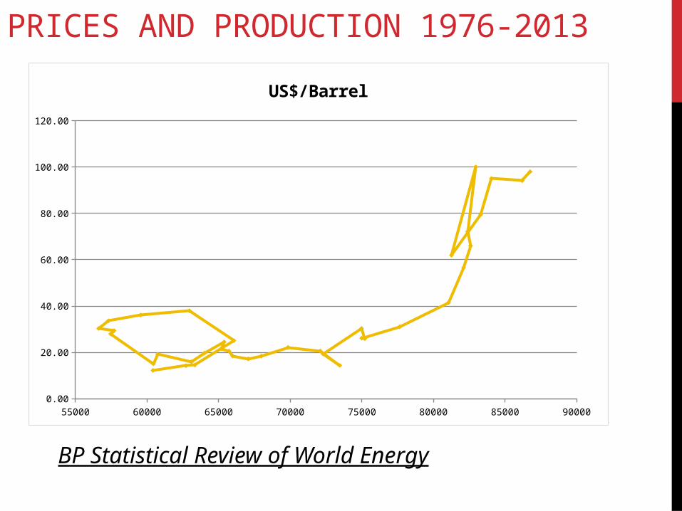
PRICES AND PRODUCTION 1976-2013

BP Statistical Review of World Energy

55000 60000 65000 70000 75000 80000 85000 900000.00

20.00

40.00

60.00

80.00

100.00

120.00

US$/Barrel

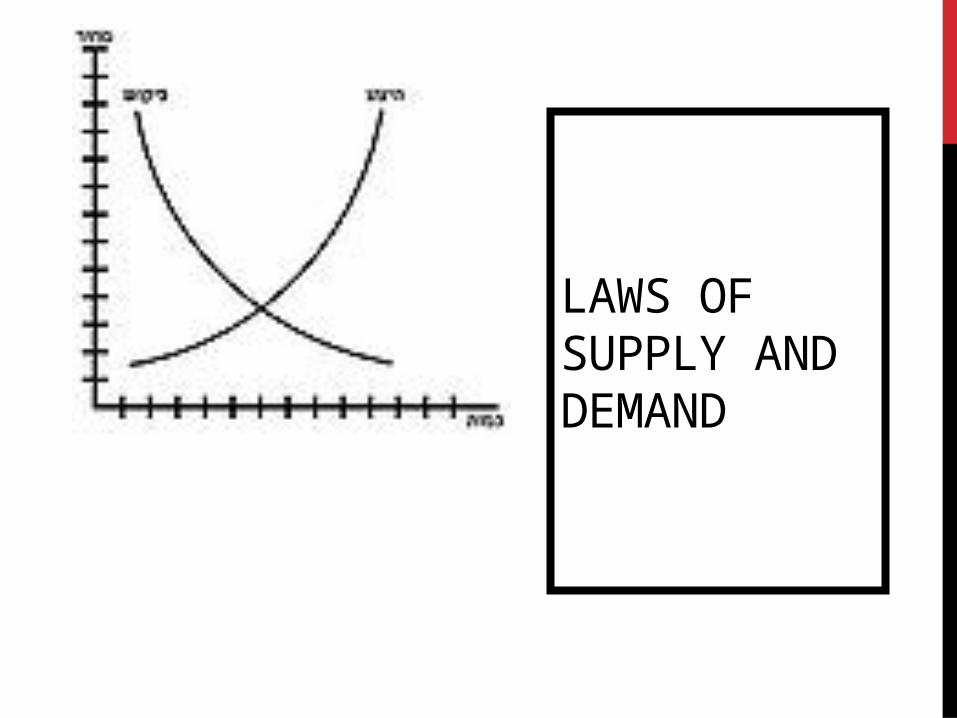
LAWS OF SUPPLY AND DEMAND

SUPPLY AND DEMAND FRAMEWORK

A description of a market includes the quantity of goods that are sold in that market, Q, and the price, P, at which they are sold.

Outcomes in the market are a function of the laws of supply and demand

LAW OF DEMAND

Ceteris parabis, There is an inverse relationship between the price of a good and the quantity that consumers would like to purchase.

What does Ceteris Parabis mean?

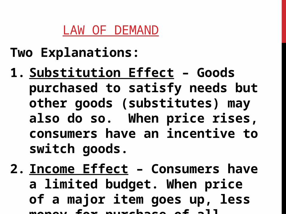
LAW OF DEMAND

Two Explanations:

1. Substitution Effect – Goods purchased to satisfy needs but other goods (substitutes) may also do so. When price rises, consumers have an incentive to switch goods.

2. Income Effect – Consumers have a limited budget. When price of a major item goes up, less money for purchase of all items.

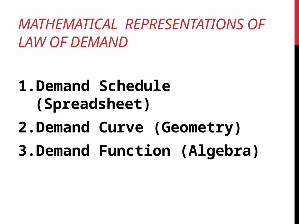
MATHEMATICAL REPRESENTATIONS OF LAW OF DEMAND

1. Demand Schedule (Spreadsheet)

2. Demand Curve (Geometry)

3. Demand Function (Algebra)

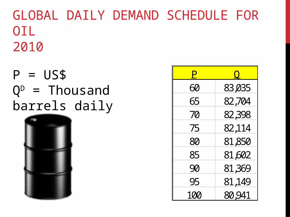
GLOBAL DAILY DEMAND SCHEDULE FOR OIL2010

P = US$QD = Thousand barrels daily

P Q60 83,03565 82,70470 82,39875 82,11480 81,85085 81,60290 81,36995 81,149100 80,941

80,500 81,000 81,500 82,000 82,500 83,000 83,50058

63

68

73

78

83

88

93

98

103

Demand Curve for Oil

Q

P

GENERAL DEMAND CURVE

DP

Q

P1

Q2

P2

Q1

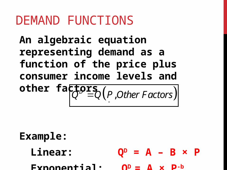
DEMAND FUNCTIONS

An algebraic equation representing demand as a function of the price plus consumer income levels and other factors

Example:

Linear: QD = A – B × P

Exponential: QD = A × P-b

,DQ Q P Other Factors

NATURAL LOGARITHM

Common for professional economists to deal with prices and quantities in natural logarithms

z = ln(Z)

z

Z

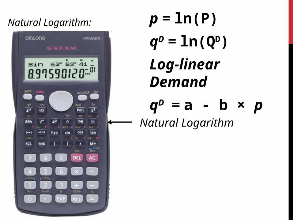
p = ln(P)

qD = ln(QD)

Log-linear Demand

qD = a - b × p

Natural Logarithm:

Natural Logarithm

LAW OF SUPPLY:

• Ceteris parabis, there is a positive relationship between the price of a good and the quantity producers bring to the market.

LAW OF SUPPLY

Explanation

Increasing Costs Producers will bring goods to market only if the price obtained from selling an extra good will exceed the cost of producing an extra good. If per unit production costs are rising in the number of goods produced, higher prices will be demanded to bring a larger quantity of goods to market.

MATHEMATICAL REPRESENTATION OF LAW OF SUPPLY

1. Supply Schedule (Spreadsheet)

2. Supply Curve (Geometry)

3. Supply Function (Algebra)

GLOBAL DAILY SUPPLY SCHEDULE FOR OIL2010

P Q60 81,35065 81,61170 81,85475 82,08080 82,29285 82,49290 82,68095 82,860100 83,030

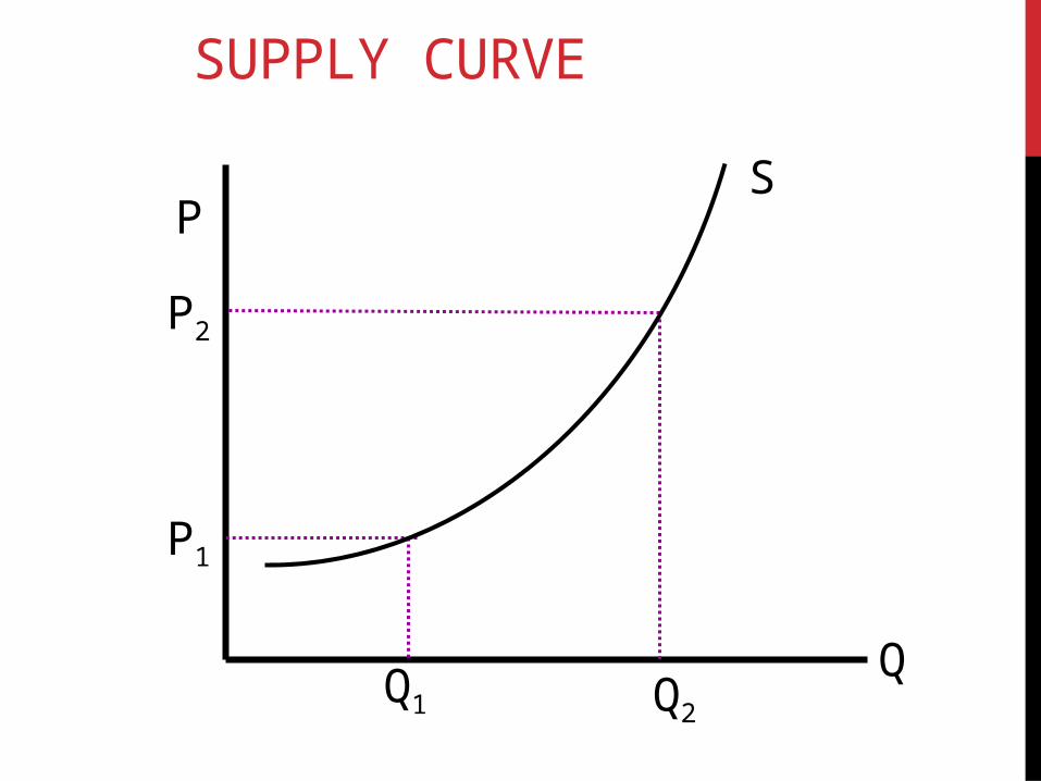
SUPPLY CURVE

SP

Q

P1

Q2

P2

Q1

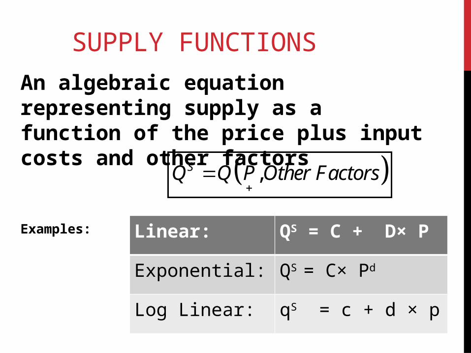
SUPPLY FUNCTIONS

An algebraic equation representing supply as a function of the price plus input costs and other factors

Examples:

,SQ Q P Other Factors

Linear: QS = C + D× P

Exponential: QS = C× Pd

Log Linear: qS = c + d × p

ELASTICITY AS PRICE SENSITIVITY

PRICE ELASTICITY: THE % IMPACT ON QUANTITY DEMANDED/SUPPLIED OF A 1% CHANGE IN PRICE

%0

% in

DDemand Drop in Q

elasticityIncrease P

%0

%

SSupply Increase in Q

elasticityIncrease in P

MIDPOINT METHODIf you want to calculate a % difference between two points which is the same regardless of which you designate as the reference point (denominator), you can use the average of the two points as the reference point.

DEMAND ELASTICITY

Rise Drop in % Rise % Drop inin Quantity in Quantity

P Q Price Demanded Price Demanded Elasticity

60 83,03562.5 82,870 5 332 8.00% 0.40% 0.050

65 82,70467.5 82,551 5 306 7.41% 0.37% 0.050

70 82,39872.5 82,256 5 284 6.90% 0.34% 0.050

75 82,11477.5 81,982 5 265 6.45% 0.32% 0.050

80 81,85082.5 81,726 5 248 6.06% 0.30% 0.050

85 81,60287.5 81,485 5 233 5.71% 0.29% 0.050

90 81,36992.5 81,259 5 220 5.41% 0.27% 0.050

95 81,14997.5 81,045 5 208 5.13% 0.26% 0.050

100 80,941

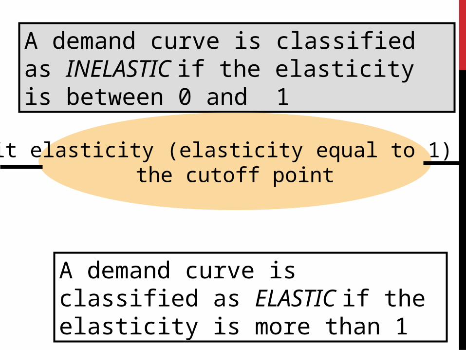
A demand curve is classified as INELASTIC if the elasticity is between 0 and 1

A demand curve is classified as ELASTIC if the elasticity is more than 1

Unit elasticity (elasticity equal to 1) is the cutoff point

PRICES AND REVENUE

Revenue in a market is Revenue = P∙Q

If prices change, revenue will change for two reasons:

1. Direct Effect of the Price Change (positive)

2. Indirect Effect of the Price Change on Quantity Demanded (negative)

Rule of Thumb: The percentage change in the product of two variables is approximately the sum of the % change in each variable.

PRICE ELASTICITY OF REVENUE

% % P %

% %1 1

% P % P

Revenue Q

Revenue Qelasticity

If demand is elastic, a price rise reduces revenues

If demand is inelastic, a price rise increases revenues

Differences in logarithms approximate midpoint measure of % changes

z1 – z0 ≡ ln(Z1) – ln(Z0) ≈ %Z/100

% Rise % Drop in Rise Dropin Quantity in in

P Q p q Price Demanded p q

60 83,035 4.094345 11.3270224

62.5 82,870 8.0% 0.4% 0.080 0.004 0.05

65 82,704 4.174387 11.3230202

67.5 82,551 7.4% 0.4% 0.074 0.004 0.05

70 82,398 4.248495 11.3193148

72.5 82,256 6.9% 0.3% 0.069 0.003 0.05

75 82,114 4.317488 11.3158652

77.5 81,982 6.5% 0.3% 0.065 0.003 0.05

80 81,850 4.382027 11.3126383

82.5 81,726 6.1% 0.3% 0.061 0.003 0.05

85 81,602 4.442651 11.309607

87.5 81,485 5.7% 0.3% 0.057 0.003 0.05

90 81,369 4.49981 11.3067491

92.5 81,259 5.4% 0.3% 0.054 0.003 0.05

95 81,149 4.553877 11.3040457

97.5 81,045 5.1% 0.3% 0.051 0.003 0.05

100 80,941 4.60517 11.3014811

EQUILIBRIUM

Equilibrium in the competitive market occurs when the price is set at a level (P*) such that the amount that consumers want to buy is equal to the amount that sellers want to sell (Q*).

Excess Supply If P were above equilibrium, sellers would want to sell more goods than buyers would want to buy. Competition between sellers would force prices down.

Excess Demand If P were below equilibrium, customers would want to buy more goods than people would want to sell. Competition between buyers would force prices up.

COMPETITIVE MARKET EQUILIBRIUM

SDP

Q

P*

Q*

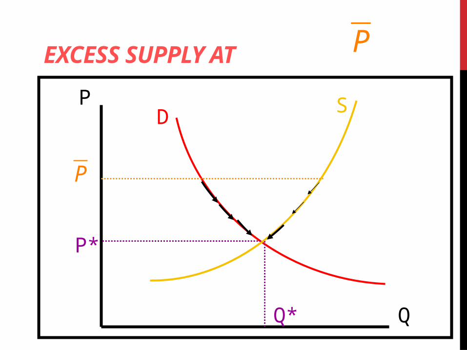
EXCESS SUPPLY AT

P

SD

P

Q

P*

Q*

P

EXCESS DEMAND AT

P

SD

P

Q

P*

Q*

P

MARKET EQUILIBRIUM(SPREADSHEET PROBLEM)At what price and quantity (to closest $5) will the oil market clear?

P QD QS60 83,035 81,35065 82,704 81,61170 82,398 81,85475 82,114 82,08080 81,850 82,29285 81,602 82,49290 81,369 82,68095 81,149 82,860100 80,941 83,030

ALGEBRA OF EQUILIBRIUM

Log Linear Functions

C + D ×P

(A-C) = (B+D) ×P*

𝑃∗=𝐴−𝐶𝐵+𝐷

A - B×P = QD QS = =

A - B×P* = C+D×P*

QS = C+D×P* = C+D×

= C×+A×

EXAMPLE

50 5

10 5 10 5 50 5

50 10 10 40 10 4

10 5 4 30

50 5 4 30

D

S

S

D

Q P

Q P P P

P P P

Q P

Q P

ALGEBRA OF EQUILIBRIUM

Log Linear Functions

c + d ×p

(a-c) = (b+d) ×p*

𝑝∗=𝑎−𝑐𝑏+𝑑

a - b×p = qD qS = =

a - b×p* = c+d×p*

qS = c+d×p* = c+d× c×+a×

ALGEBRA OF EQUILIBRIUM

Log Linear Functions

11.14 + .04 ×p

(11.53-11.14) = (.05+.04) ×p* =4.333

11.53 - .05×p= qD qS = =

11.53 - .05×p* = 11.14+.04×p*

qS = 11.14+.04×4.3333 = 11.316

ALGEBRA OF EQUILIBRIUMLog Linear Functions

qD = 11.53 - .05×pqS = 11.14 + .04 ×p

11.53 - .05×p* = 11.14+.04×p* (.39) = .09 ×p*.39.09

=4.333=𝑝∗

3=11.316

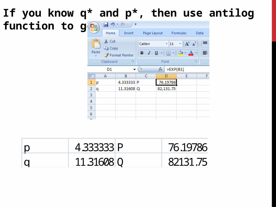
If you know q* and p*, then use antilog function to get Q* and P*

p 4.333333 P 76.19786q 11.31608 Q 82131.75

MARKET CHANGES:SHIFTS IN DEMAND & SUPPLY CURVES

SHIFTING CURVES/CHANGING EQUILIBRIUMChanges in equilibrium result from shifts in either the demand or supply schedule. We think of shifts in the curves as changes in supply or demand that are caused by factors other than changes in the price of the good.

• Shifts in the demand curve lead to movements along the supply curve resulting in changes in prices and quantities that move in the same direction.

• Shifts in the supply curve lead to movements along the demand curve resulting in changes in prices and quantities that move in different directions.

A SHIFT IN THE DEMAND CURVE: A PARALLEL INCREASE IN THE DEMAND SCHEDULE AT EVERY PRICE POINT.PRICE AND QUANTITY DEMANDED MOVE IN SAME DIRECTION

S

D

P

Q

P*

Q*

P**

Q**

D′

Shift in the demand curve

⓪

①

Excess Demand

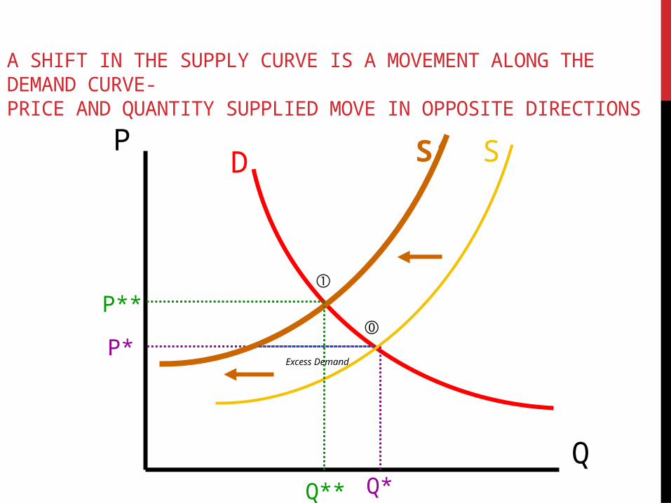
A SHIFT IN THE SUPPLY CURVE IS A MOVEMENT ALONG THE DEMAND CURVE- PRICE AND QUANTITY SUPPLIED MOVE IN OPPOSITE DIRECTIONS

SDP

Q

P*

Q*

P**

Q**

S′

⓪

①

Excess Demand

EQUILIBRIUM EFFECTS

Price system means that shifts in demand will cause accommodating changes in quantity supplied but also an attenuating change in quantity demanded.

Shifts in supply will cause accommodating changes in quantity demanded but also attenuating change in quantity supplied.

EQUILIBRIUM EFFECT: MOVEMENT ALONG THE SUPPLY CURVE INCREASES QUANTITY SUPPLIED; MOVEMENT ALONG DEMAND CURVE AMELIORATES QUANTITY DEMANDED.

S

D

P

Q

P*

Q*

P**

Q**

D′⓪

①

Excess Demand

Along supply curve

Along demand curve

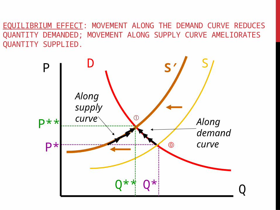
EQUILIBRIUM EFFECT: MOVEMENT ALONG THE DEMAND CURVE REDUCES QUANTITY DEMANDED; MOVEMENT ALONG SUPPLY CURVE AMELIORATES QUANTITY SUPPLIED.

SDP

Q

P*

Q*

P**

Q**

S′

Along supply curve Along demand

curve⓪

①

WHAT SHIFTS THE CURVES?

WHAT SHIFTS THE

DEMAND CURVE?

1. Price of Related Goods

2. Income

3. Consumer Preferences

4. Expected Future Prices

5. Expected Future Income

WHAT SHIFTS THE

SUPPLY CURVE?

1. Price of Inputs

2. Price of Related Goods

3. Technology/Nature

4. Expected Future Prices

5. Market Entry

CHANGING EQUILIBRIUM

INCOME ELASTICITY/ CROSS PRICE ELASTICITY

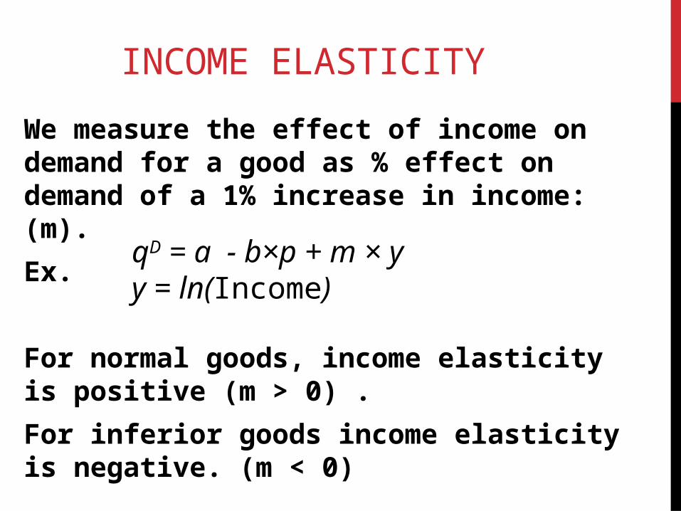
INCOME ELASTICITY

We measure the effect of income on demand for a good as % effect on demand of a 1% increase in income: (m).

Ex.

For normal goods, income elasticity is positive (m > 0) .

For inferior goods income elasticity is negative. (m < 0)

qD = a - b×p + m × y y = ln(Income)

LUXURIES VS. NECESSITIES

There are two types of normal goods.

Luxuries take up an increasing share of income as your income grows.

• Luxuries are income elastic - the income elasticity of luxuries is greater than 1 (m > 1).

Necessities take up a declining share of income as your income grows.

• Necessities are income inelastic – the income elasticity of necessities is less than 1 (0 < m < 1).

China’s Emerging Middle Class Download

RANGE OF INCOME ELASTICITIES

0 1

Inferior Goods

Normal Goods

Income Elastic (Luxury Goods)

Income Inelastic (Necessities)

CHANGES IN PRICES OF OTHER GOODSFor any good there are two types of other

goods which are relevant to its demand

1. Substitutes: Those other goods which can take the place of the good of interest (bacon vs. ham)

2. Complements: Those other goods whose use will enhance the value of the good of interest. (bacon and eggs)

What are substitutes and complements for oil

SUBSTITUTES VS. COMPLEMENTS

A good is defined as a “Substitute” when a rise in its price leads to a shift out/up in the demand curve for the good of interest.

A good is defined as a “Complement” when a rise in its price leads to a shift in/down in the demand curve for the good of interest.

CROSS PRICE ELASTICITYCross price elasticity is the % effect on the quantity demanded of a % change in another price.

• Goods with positive cross-price elasticities are called substitutes

• Goods with negative cross-price elasticities are called complements

0

SubstitutesComplements

CROSS PRICE ELASTICITYWe measure the effect of income on demand for a good as % effect on demand of a 1% increase in related price: f.

Ex.

For substitutes, cross price elasticity is positive (f > 0).

For complements , cross price elasticity is negative (f < 0).

qD = a - b×p + f × pk pk = ln(Price of Related Good)

COMMODITY MARKETS

CHAP. 3, 4

OIL PRICES

Link

Why are commodity prices so volatile?

PRICE SENSITIVITY AND EQUILIBRIUM EFFECTS

When supply or demand curves shift, the effect will be felt in some combination of changes in prices and quantities.

The degree to which changes in either supply or demand are felt in quantity changes rather than price changes is determined by price sensitivity of both demand and supply.

WHAT DETERMINES PRICE ELASTICITY?

AVAILABILITY OF SUBSTITUTES

A price increase will lead to a shift away from the use of a product and toward other products.

• Price elasticity will be stronger if there are readily available substitutes for a good.

SHARE OF INCOMEA price increase for one good reduce income available for purchases for all goods

• Price elasticity will be stronger if a good makes up a big chunk of income.

World Bank Tobacco Download

COMPARISONS OF DEMAND PRICE ELASTICITIES

Salt .1Coffee .25

Tobacco .45

Movies .9

Housing 1.2

Restaurant Meals 2.3

Commodities have very inelastic demand.

• Estimate of elasticity of demand for oil in the US is .061 J.C.B. Cooper, OPEC Review, 2003)

Price Elasticities of Other Goods

ELASTICITIES EXTREME

Perfectly Inelastic Demand (Insulin)

Perfectly Elastic Demand (Clear Pepsi)

P

Q

D

D

.

P

QQ*

S'

P*

D2

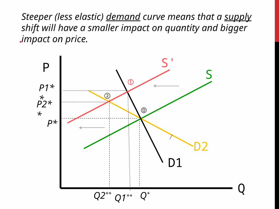
Steeper (less elastic) demand curve means that a supply shift will have a smaller impact on quantity and bigger impact on price.

D1

S

Q2**

P1**

Q1**

P2**⓪

①

②

ELASTICITY OF SUPPLY

Elasticity of supply curve depends on the ability of production sector to ramp up supply without increasing the marginal cost of production.

A good that is produced with readily available factors w/o a need for time consuming investment will have an elastic supply curve.

ELASTICITIES: SUPPLY

Perfectly Inelastic Supply

(Van Gogh Paintings)

Perfectly Elastic Supply (Foot Massage)

P

Q

S

S

.

P

QQ*

S1

P*

D

Steeper (less price sensitive) supply curve means that a demand shift will have a smaller impact on quantity and bigger impact on price.

D'

S2

Q1**

P1**

Q2**

P2** ⓪

①

②

ALGEBRA OF EQUILIBRIUM EFFECTS

If demand or supply elasticities are big, effects of supply or demand change on equilibrium price will be small

1*

1*

a p ab d

c p cb d

*a c

pb d b d

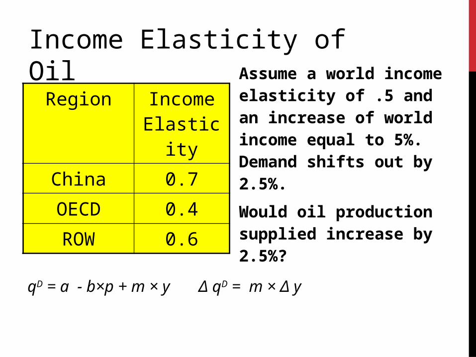
SOURCE: OECD STUDY

Region Income Elasticity

China 0.7

OECD 0.4

ROW 0.6

Assume a world income elasticity of .5 and an increase of world income equal to 5%. Demand shifts out by 2.5%.

Would oil production supplied increase by 2.5%?

Income Elasticity of Oil

qD = a - b×p + m × y Δ qD = m × Δ y

MARKET EQUILIBRIUM(SPREADSHEET PROBLEM)

At what price and quantity (to closest $5) will the oil market clear?

P QD QD´ QS

60 83,035 85,111 81,35065 82,704 84,771 81,61170 82,398 84,458 81,85475 82,114 84,167 82,08080 81,850 83,896 82,29285 81,602 83,642 82,49290 81,369 83,403 82,68095 81,149 83,178 82,860100 80,941 82,965 83,030

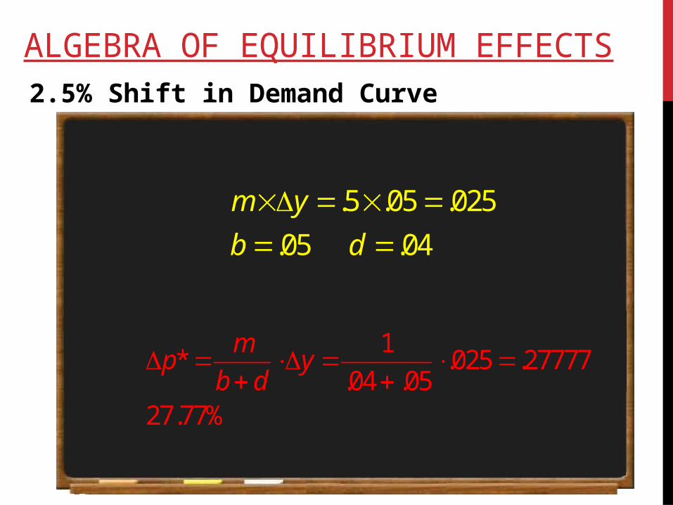
ALGEBRA OF EQUILIBRIUM EFFECTS2.5% Shift in Demand Curve

.5 .05 .025

.05 .04

m y

b d

1* .025 .27777

.04 .0527.77%

mp y

b d

PRICE ELASTICITY AND TIME

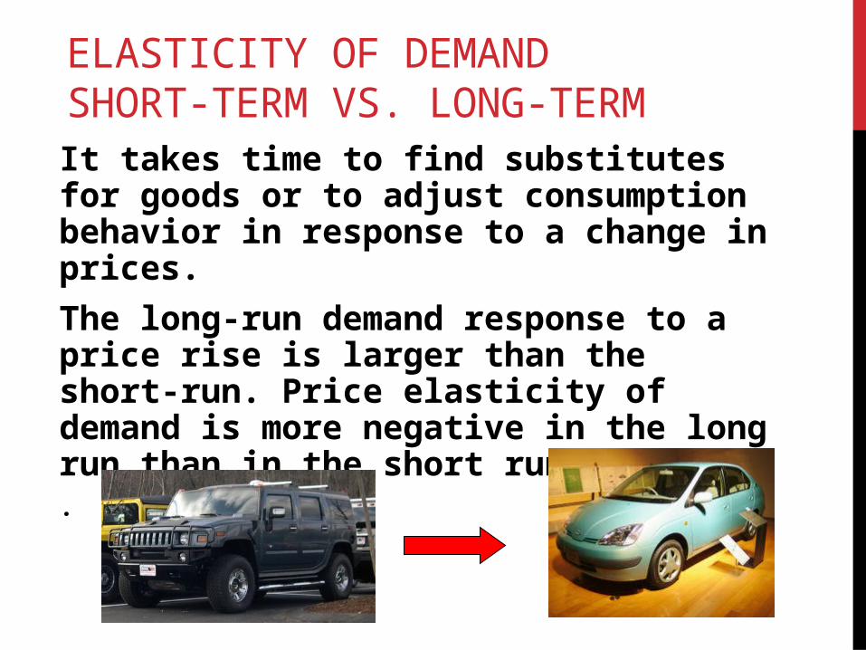
ELASTICITY OF DEMAND SHORT-TERM VS. LONG-TERMIt takes time to find substitutes for goods or to adjust consumption behavior in response to a change in prices.

The long-run demand response to a price rise is larger than the short-run. Price elasticity of demand is more negative in the long run than in the short run. .

OIL DEMAND MUCH MORE ELASTIC IN LONG RUN THAN SHORT-RUN

Price Elasticity of DemandShort-term Long-term

Germany 0.02 0.27Japan 0.07 0.36Korea 0.09 0.18USA 0.06 0.45

– (J.C.B. Cooper, OPEC Review, 2003)

PRICE ELASTICITY OF SUPPLY

Firms also find it easier to adjust production in the long-run than the short run. Long-run price elasticity of supply is typically greater than short-run

OECD study suggests price elasticity of oil supply is .04 in short run and .35 in long run.

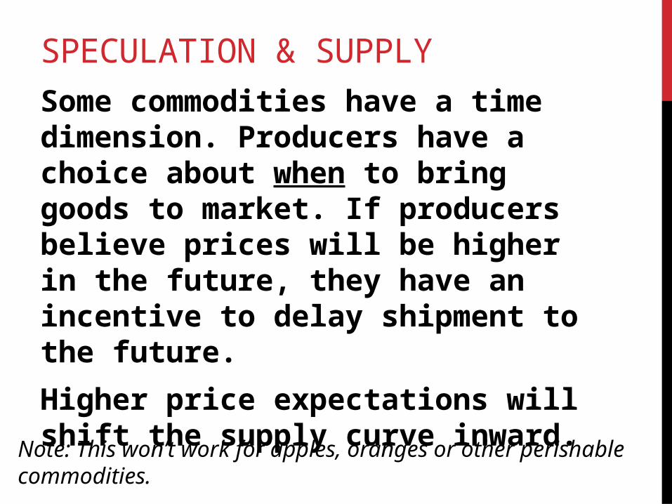
SPECULATION & SUPPLY

Some commodities have a time dimension. Producers have a choice about when to bring goods to market. If producers believe prices will be higher in the future, they have an incentive to delay shipment to the future.

Higher price expectations will shift the supply curve inward.

Note: This won’t work for apples, oranges or other perishable commodities.

EXPECTATIONS OF INCREASED PRICES IN THE FUTURE LEAD TO HIGHER PRICES TODAY!

SDP

Q

P*

Q*

P**

Q**

S′

⓪

①

CONTANGO

CLY00

(Cas

h)

CLJ15

(Apr

'15)

CLN15

(Jul

'15)

CLV15

(Oct

'15)

CLF16

(Jan

'16)

CLJ16

(Apr

'16)

CLN16

(Jul

'16)

CLV16

(Oct

'16)

CLF17

(Jan

'17)

CLJ17

(Apr

'17)

CLN17

(Jul

'17)

CLV17

(Oct

'17)

CLF18

(Jan

'18)

CLJ18

(Apr

'18)

CLN18

(Jul

'18)

CLV18

(Oct

'18)

CLF19

(Jan

'19)

CLJ19

(Apr

'19)

CLN19

(Jul

'19)

CLV19

(Oct

'19)

CLF20

(Jan

'20)

CLJ20

(Apr

'20)

CLN20

(Jul

'20)

CLV20

(Oct

'20)

CLM21

(Jun

'21)

CLZ22

(Dec

'22)

50

55

60

65

70

75

NYMEX WTI Futures US$/Bbl

Last

SPECULATION & DEMAND

For some storable commodities (e.g. gold) or durable goods, expectations of future price hikes might also lead consumers to start buying immediately.

Higher price expectations will shift demand curve outward.

EVEN HIGHER PRICES!

SDP

Q

P*

Q***

P**

Q**

S'D'

P***

⓪

①

②

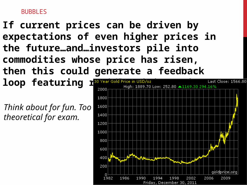
BUBBLES

If current prices can be driven by expectations of even higher prices in the future…and…investors pile into commodities whose price has risen, then this could generate a feedback loop featuring rapidly rising prices

Think about for fun. Too theoretical for exam.

BUBBLE BURSTS?

St. Louis Fed Database

EXPECTED INCOME EFFECT

Households are forward looking. If they expect income in the future they will increase spending today.

Optimism (or pessimism) about future income will shift demand curve.

LEARNING OUTCOMES

Solve for equilibrium price and quantities using graphical supply and demand model or spreadsheet supply and demand schedules or simple linear algebra.

Explain qualitatively and calculate quantitatively, the likely consequences for equilibrium prices and quantities resulting from exogenous shifts in supply and demand.

Calculate elasticities using the midpoint method.

LEARNING OUTCOMES

Distinguish substitutes/complements, luxuries/necessities/inferior goods.

Identify the impact of demand & supply elasticity on price and quantity volatility in the short and long run.

Identify the impact of expectations of the future on current prices.