Supplementary Methods. Testing phylogenetic independent origin hypotheses using Bayes factors Abstract To assess support for the hypothesis that photophores originated more than once, we developed a Bayes factor test in which we compare the prior and posterior probabilities of the observed data under two opposing hypotheses (that the number of gains required is either less than or greater/equal to M ). To approximate these prior and posterior probabilities we developed a computational method which uses MCMC to account for phylogenetic uncertainty and uncertainty in rates of gain and loss. Here we describe the model assumptions and computational details, which have been implemented in the R package indorigin available at https://github.com/vnminin/indorigin. Modeling assumptions We start with a binary character (e.g. absence/presence of a morphological trait) measured in n species. We collect these measurements into vector y =(y 1 ,...,y n ), where each y i ∈{0, 1}. Suppose that the evolutionary relationship among the above species can be described by a phylogeny τ , which includes branch lengths. We assume that the binary character had evolved along this phylogeny according to a two-state continuous-time Markov chain (CTMC) with an infinitesimal rate matrix Λ = -λ 01 λ 01 λ 10 -λ 10 . We also assume that we have another set of data x, molecular and/or morphological, collected from the same species. In principle, we can set up an evolutionary model for this second data set, with evolutionary model parameters θ (e.g. substitution matrix, rate heterogeneity pa- rameters) and then approximate the posterior distribution of all model parameters conditional on all available data: Pr(τ, θ,λ 01 ,λ 10 | x, y) ∝ Pr(x | τ, θ)Pr(y | τ,λ 01 ,λ 10 )Pr(τ )Pr(θ)Pr(λ 01 )Pr(λ 10 ), (1) where we assume that a priori λ 01 ∼ Gamma(α 01 ,β 01 ) and λ 10 ∼ Gamma(α 10 ,β 10 ), with the rest of the priors left unspecified for generality. However, in practice the contribution of the data vector y to phylogenetic estimation is negligible when compared to the contribution of the data matrix x. Therefore, we take a two-stage approach, where we first approximate the posterior distribution Pr(τ, θ | x) ∝ Pr(x | τ, θ)Pr(τ )Pr(θ)Pr(λ 01 )Pr(λ 10 ) via Markov chain Monte Carlo (MCMC). This produces the posterior sample of K phylogenies, τ =(τ 1 ,...,τ K ). This sample can also be generated via a bootstrap procedure within the maximum likelihood analysis. Next, we form an approximate posterior distribution f Pr(λ 01 ,λ 10 | x, y)= Z τ Pr(λ 01 ,λ 10 | τ, y)Pr(τ | x)dτ ∝ Z τ Pr(y | τ,λ 01 ,λ 10 )Pr(λ 01 )Pr(λ 10 )Pr(τ | x)dτ ≈ " K X k=1 Pr(y | τ k ,λ 01 ,λ 10 ) # Pr(λ 01 )Pr(λ 10 ). (2) 1

Welcome message from author
This document is posted to help you gain knowledge. Please leave a comment to let me know what you think about it! Share it to your friends and learn new things together.
Transcript

Supplementary Methods. Testing phylogenetic independentorigin hypotheses using Bayes factors
Abstract
To assess support for the hypothesis that photophores originated more than once, wedeveloped a Bayes factor test in which we compare the prior and posterior probabilitiesof the observed data under two opposing hypotheses (that the number of gains requiredis either less than or greater/equal to M). To approximate these prior and posteriorprobabilities we developed a computational method which uses MCMC to account forphylogenetic uncertainty and uncertainty in rates of gain and loss. Here we describe themodel assumptions and computational details, which have been implemented in the Rpackage indorigin available at https://github.com/vnminin/indorigin.
Modeling assumptions
We start with a binary character (e.g. absence/presence of a morphological trait) measured inn species. We collect these measurements into vector y = (y1, . . . , yn), where each yi ∈ {0, 1}.Suppose that the evolutionary relationship among the above species can be described by aphylogeny τ , which includes branch lengths. We assume that the binary character had evolvedalong this phylogeny according to a two-state continuous-time Markov chain (CTMC) with aninfinitesimal rate matrix
Λ =
(−λ01 λ01λ10 −λ10
).
We also assume that we have another set of data x, molecular and/or morphological, collectedfrom the same species. In principle, we can set up an evolutionary model for this second dataset, with evolutionary model parameters θ (e.g. substitution matrix, rate heterogeneity pa-rameters) and then approximate the posterior distribution of all model parameters conditionalon all available data:
Pr(τ,θ, λ01, λ10 | x,y) ∝ Pr(x | τ,θ)Pr(y | τ, λ01, λ10)Pr(τ)Pr(θ)Pr(λ01)Pr(λ10), (1)
where we assume that a priori λ01 ∼ Gamma(α01, β01) and λ10 ∼ Gamma(α10, β10), with therest of the priors left unspecified for generality. However, in practice the contribution of thedata vector y to phylogenetic estimation is negligible when compared to the contribution ofthe data matrix x. Therefore, we take a two-stage approach, where we first approximate theposterior distribution
Pr(τ,θ | x) ∝ Pr(x | τ,θ)Pr(τ)Pr(θ)Pr(λ01)Pr(λ10)
via Markov chain Monte Carlo (MCMC). This produces the posterior sample of K phylogenies,τ = (τ1, . . . , τK). This sample can also be generated via a bootstrap procedure within themaximum likelihood analysis. Next, we form an approximate posterior distribution
Pr(λ01, λ10 | x,y) =
∫τ
Pr(λ01, λ10 | τ,y)Pr(τ | x)dτ
∝∫τ
Pr(y | τ, λ01, λ10)Pr(λ01)Pr(λ10)Pr(τ | x)dτ
≈
[K∑k=1
Pr(y | τk, λ01, λ10)
]Pr(λ01)Pr(λ10).
(2)
1

that helps us estimate the rates of gain and loss of the trait, λ01 and λ10, appropriately ac-counting for phylogenetic uncertainty. The approximate posterior (2) has only two parametersand therefore can be approximated by multiple numerical procedures, including deterministicintegration techniques, such as Gaussian quadrature. We implement a MCMC algorithm thattargets posterior (2), but plan to experiment with deterministic integration in the future.
So far our modeling assumptions and approximations follow standard practices in statisticalphylogenetics as applied to macroevolution. For example, one could use software packagesBayesTraits [Pagel et al., 2004] or Mr.Bayes [Ronquist et al., 2012], among many others, toapproximate the posterior distributions (1) or (2). The main novelty of our methodology,explained in the next section, comes from the way we use these posteriors to devise a principledmethod for testing hypotheses about the number of gains and losses of the trait of interest.
Hypotheses and their Bayes factors
Let N01 be the number of gains and let N10 be the number of losses. Conservatively, in thiswork we assume that the root of the phylogenetic tree relating the species under study is instate 1. This means that the parsimony score for the number of gains associated with vector yand any phylogeny is 0, because under our assumption about the root any binary vector canbe generated with only trait losses, even though such an evolutionary trajectory may be veryunlikely.
We fix a nonnegative thresholdm and formulate an independent origin hypothesis associatedwith this threshold as
H0 : N01 ≤M,
with the corresponding alternativeHa : N01 > M.
This means that our null hypothesis is that the trait was gained at most M + 1 times — weadd one because we know that the trait was gained at least once. For example, using M = 0corresponds to testing the null hypothesis that the trait was gained only once some time priorto the time of the most recent common ancestor of the species under study. We use a Bayesfactor test [Kass and Raftery, 1995] to compare the above two hypotheses:
BFM =Pr(y | N01 ≤M)
Pr(y | N01 > M)=
Pr(N01 ≤M | y)/Pr(N01 ≤M)
Pr(N01 > M | y)/Pr(N01 > M), (3)
where Pr(N01 ≤ M | y) and Pr(N01 > M | y) are the posterior probabilities of the nulland alternative hypotheses, and Pr(N01 ≤ M) and Pr(N01 > M) are the corresponding priorprobabilities. We explain how we compute these probabilities in the next section.
Computational details
We approximate the posterior (2) by a MCMC algorithm that starts with arbitrary initial
values λ(0)01 , λ
(0)01 and at each iteration l ≥ 1 repeats the following steps:
1. Sample uniformly at random a tree index k from the set {1, . . . ,K} and set the currenttree τ (l) = τk.
2
2. Conditional on the phylogeny and the gain and loss rates from the previous iteration,draw a realization of the full evolutionary trajectory (also known as stochastic mapping[Nielsen, 2002]) on phylogeny τ (l) using the uniformization method [Lartillot, 2006] and
record the following missing data summaries: N(l)01 , N
(l)10 , defined as before, and t
(l)0 , t
(l)1
— total times the trait spent in state 0 and 1 respectively.
3. Draw new values of gain and loss rates from their full conditionals:
λ(l)01 ∼ Gamma(N
(l)01 + α01, t
(l)0 + β01),
λ(l)10 ∼ Gamma(N
(l)10 + α10, t
(l)1 + β10).
Advantages of using the above Gibbs sampling algorithm are: a) no tuning is required and b)augmenting the state space with latent variables, N01, N10, t0, t1, and sampling these latentvariables efficiently yield rapid convergence of the MCMC, in our experience.
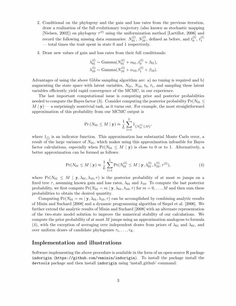
The last important computational issue is computing prior and posterior probabilitiesneeded to compute the Bayes factor (3). Consider computing the posterior probability Pr(N01 ≤M | y) — a surprisingly nontrivial task, as it turns out. For example, the most straightforwardapproximation of this probability from our MCMC output is
Pr (N01 ≤M | y) ≈ 1
L
L∑l=1
1{N(l)01 ≤M}
,
where 1{} is an indicator function. This approximation has substantial Monte Carlo error, aresult of the large variance of N01, which makes using this approximation infeasible for Bayesfactor calculations, especially when Pr(N01 ≤ M | y) is close to 0 or to 1. Alternatively, abetter approximation can be formed as follows:
Pr(N01 ≤M | y) ≈ 1
L
L∑l=1
Pr(N(l)01 ≤M | y, λ
(l)01 , λ
(l)10 , τ
(l)), (4)
where Pr(N01 ≤ M | y, λ01, λ10, τ) is the posterior probability of at most m jumps on afixed tree τ , assuming known gain and loss rates, λ01 and λ10. To compute the last posteriorprobability, we first compute Pr(N01 = m | y, λ01, λ10, τ) for m = 0, . . . ,M and then sum theseprobabilities to obtain the desired quantity.
Computing Pr(N01 = m | y, λ01, λ10, τ) can be accomplished by combining analytic resultsof Minin and Suchard [2008] and a dynamic programming algorithm of Siepel et al. [2006]. Wefurther extend the analytic results of Minin and Suchard [2008] with an alternate representationof the two-state model solution to improve the numerical stability of our calculations. Wecompute the prior probability of at mostM jumps using an approximation analogous to formula(4), with the exception of averaging over independent draws from priors of λ01 and λ01, andover uniform draws of candidate phylogenies τ1, . . . , τK .
Implementation and illustrations
Software implementing the above procedure is available in the form of an open-source R packageindorigin (https://github.com/vnminin/indorigin). To install the package install thedevtools package and then install indorigin using ‘install github’ command:
3

## install.packages("devtools") # uncomment if "devtoos" is not installed
## install_github("vnminin/indorigin") # uncomment or copy and paste into R terminal
library(indorigin)
## Loading required package: Rcpp
## Loading required package: RcppArmadillo
## Loading required package: testthat
Notice that installing from github requires installing the package from source. To learnabout package installation see http://cran.r-project.org/doc/manuals/R-admin.html.
Simulated data
Let’s simulate a tree and fast/slow evolving binary traits on this tree.
library(diversitree) # diversitree is only needed for simulations
## Loading required package: deSolve
## Loading required package: ape
## Loading required package: subplex
## Loading required package: methods
set.seed(3245)
## Simulate a tree
phy<-NULL
while(is.null(phy)){phy <- tree.bd(c(.1, .03), max.taxa=50)
}
## Simulate FAST EVOLVING 0/1 characters on this tree
states1 <- sim.character(phy, c(.03, .1), x0=1, model="mk2")
## Simulate SLOW EVOLVING 0/1 characters on this tree
states2 <- sim.character(phy, c(.001, .01), x0=1, model="mk2")
First, we analyze the data simulated under the fast evolving trait regime. In this case, theBayes factor strongly rejects the hypothesis that there were 0 gains of the trait.
## run the independet origin analysis on the simulated data.
## Notice that the first argument must be a list of trees even if you are
## supplying one tree. Hence, c(phy) command.
testIndOriginResults1 = testIndOrigin(inputTrees=c(phy), traitData=states1,
initLambda01=.01, initLambda10=.01, priorAlpha01=1, priorBeta01=10,
priorAlpha10=1, priorBeta10=10, mcmcSize=2100, mcmcBurnin=100,
mcmcSubsample=1, mcSize=10000)
## pre-processing trees and trait data
4

## plot the tree with the simulated histories at all nodes
par(mfrow=c(1,2))
plot(phy, show.tip.label=FALSE, no.margin=TRUE)
col <- c("#004165", "#eaab00")
tiplabels(col=col[states1+1], pch=19, adj=1)
nodelabels(col=col[attr(states1, "node.state")+1], pch=19)
plot(phy, show.tip.label=FALSE, no.margin=TRUE)
col <- c("#004165", "#eaab00")
tiplabels(col=col[states2+1], pch=19, adj=1)
nodelabels(col=col[attr(states2, "node.state")+1], pch=19)
●
●
●
●
●
●●
●
●●
●
●
●●
●
●
●
●
●
●
●●
●●
●●
●
●
●●
●●
●●●●
●●
●
●●
●●
●
●●
●●
●●
●
●
●
●
●
●
●
●
●
●
●
●
●
●
●
●
●
●
●
●
●
●
●
●●
●
●
●
●
●
●
●
●
●
●
●
●
●
●
●
●
●
●
●
●
●
●
●
●
●
●
●
●
●
●●
●
●●
●
●
●●
●
●
●
●
●
●
●●
●●
●●
●
●
●●
●●
●●●●
●●
●
●●
●●
●
●●
●●
●●
●
●
●
●
●
●
●
●
●
●
●
●
●
●
●
●
●
●
●
●
●
●
●
●●
●
●
●
●
●
●
●
●
●
●
●
●
●
●
●
●
●
●
●
●
●
●
●
●
Figure 1: Fast (left figure) and slow (right figure) evolving binary traits with true internalnode states plotted.
5

## running Gibbs sampler
## Computing posterior probabilities
## Computing prior probabilities
getBF(testIndOriginResults1)
## BF for N01<=0 log10(BF) 2xlog_e(BF)
## 5.173e-06 -5.286e+00 -2.434e+01
When we perform a similar analysis for the slow evolving trait, the Bayes factor supports thehypothesis of 0 gains, but the support is very weak. This is expected, because data generatedunder the slow evolving model have very little information about the gain/loss rates, so thereis a lot of uncertainty about these rates.
testIndOriginResults2 = testIndOrigin(inputTrees=c(phy), traitData=states2,
initLambda01=.01, initLambda10=0.1, priorAlpha01=1, priorBeta01=10,
priorAlpha10=1, priorBeta10=10, mcmcSize=2100, mcmcBurnin=100,
mcmcSubsample=1, mcSize=10000)
## pre-processing trees and trait data
## running Gibbs sampler
## Computing posterior probabilities
## Computing prior probabilities
getBF(testIndOriginResults2)
## BF for N01<=0 log10(BF) 2xlog_e(BF)
## 1.11587 0.04761 0.21927
Photophores data
First, we are going to load 1000 phylogenies of 70 cephalopod species and a correspondingvector of trait values (presence/absence of photophores).
library(ape)
cephalopodTrees = read.tree("BLsonboots70.phy")
tree.num = length(cephalopodTrees)
cephalopodTraits = read.csv("BLspecies70.csv", header=FALSE)
# a little massaging to get trait data into a vector format
tip.num = dim(cephalopodTraits)[1]
cephalopodTraitVec = numeric(tip.num)
tipNames = as.character(cephalopodTraits[,1])
cephalopodTraitVec = cephalopodTraits[,2]
names(cephalopodTraitVec) = tipNames
# run the analysis
6
cephalopodIndOriginResults = testIndOrigin(inputTrees=cephalopodTrees,
traitData=cephalopodTraitVec,initLambda01=.01, initLambda10=0.1,
priorAlpha01=1, priorBeta01=100, priorAlpha10=1, priorBeta10=10,
mcmcSize=1100, mcmcBurnin=100, mcmcSubsample=1, mcSize=1000, testThreshold=2)
## pre-processing trees and trait data
## running Gibbs sampler
## Computing posterior probabilities
## Computing prior probabilities
# get the Bayes factor
getBF(cephalopodIndOriginResults)
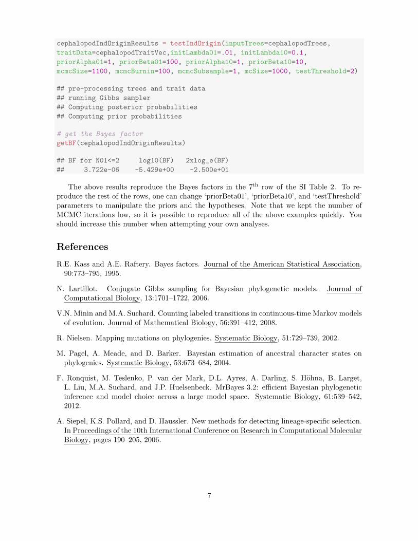
## BF for N01<=2 log10(BF) 2xlog_e(BF)
## 3.722e-06 -5.429e+00 -2.500e+01
The above results reproduce the Bayes factors in the 7th row of the SI Table 2. To re-produce the rest of the rows, one can change ‘priorBeta01’, ‘priorBeta10’, and ‘testThreshold’parameters to manipulate the priors and the hypotheses. Note that we kept the number ofMCMC iterations low, so it is possible to reproduce all of the above examples quickly. Youshould increase this number when attempting your own analyses.
References
R.E. Kass and A.E. Raftery. Bayes factors. Journal of the American Statistical Association,90:773–795, 1995.
N. Lartillot. Conjugate Gibbs sampling for Bayesian phylogenetic models. Journal ofComputational Biology, 13:1701–1722, 2006.
V.N. Minin and M.A. Suchard. Counting labeled transitions in continuous-time Markov modelsof evolution. Journal of Mathematical Biology, 56:391–412, 2008.
R. Nielsen. Mapping mutations on phylogenies. Systematic Biology, 51:729–739, 2002.
M. Pagel, A. Meade, and D. Barker. Bayesian estimation of ancestral character states onphylogenies. Systematic Biology, 53:673–684, 2004.
F. Ronquist, M. Teslenko, P. van der Mark, D.L. Ayres, A. Darling, S. Hohna, B. Larget,L. Liu, M.A. Suchard, and J.P. Huelsenbeck. MrBayes 3.2: efficient Bayesian phylogeneticinference and model choice across a large model space. Systematic Biology, 61:539–542,2012.
A. Siepel, K.S. Pollard, and D. Haussler. New methods for detecting lineage-specific selection.In Proceedings of the 10th International Conference on Research in Computational MolecularBiology, pages 190–205, 2006.
7

��� ����������� ������ ��������������������� ���������������� ������� � �"����������� ��� ����� ��"���� ��������������������� ��� ������������ � ������� ��������������������!�"������ ������� ����������� �����"�"����!�������
1
GenBank Name 12S 16S 18S ald3 ATPsyth COI cytb ef1a H3 odh opsin paxAfrololigo mercatoris 93004770 194474586 194474656Alloteuthis africana 194474470 194474508 194474600Alloteuthis media 194474490 194474550 194474634Alloteuthis subulata 194474505 194474580 194474650Argonauta nodosa 45510911 45510935 49482067 4003405 76359244 50346987 45510951 45511050Chiroteuthis calyx 209969953 209969999 209970103 0 209970211Loligo gahi 93004761 5678658 = Doryteuthis gahiLoligo opalescens 2402666124 2402666123 0 2402666121 2402666122 0 12055096 0 1778016 = Doryteuthis opalescensLoligo pealei 56567271 34369176 18026439 EF423109_1 38607257 AY450853_1 = Doryteuthis pealeiiLoligo plei 93004765 0 14120087 0 0 0 0 0 = Doryteuthis pleiEledone cirrhosa 48994420 18073265 49482072 48994473 48994575 48994529Enteroctopus dofleini 62005876 45510940 62084159 239735795 JF927838_1 0 45510965 45510966 45511018Euprymna berryi 34542045 14161379 13195587Euprymna hyllebergi 34542048 34542074 34542132Euprymna morsei 62005906 34542070Euprymna scolopes 34542046 34542072 JF927843_1 34542128 JF927842_1 48994346 48994378 21667880Euprymna tasmanica 34542047 34542073 34542130 48994587 48994541Graneledone verrucosa 45510922 82561543 49482073 4003433 50346991 45510973 158828841 45511024Heterololigo bleekeri 97906254 97906253 979062511 97906252Heteroteuthis hawaiiensis 34542063 34542089 49482077 34542160 50346997 48994344 48994376 48994406Idiosepius paradoxus 62005903 62005892 62084191 AB716344_1Loligo forbesi 45510930 498938 5678661 0 45510987 45511086 45511040Loligo reynaudii 93004766 5678665Loligo vulgaris 77157317 498939 5678656 0 13561066Loliolus beka 384228941 384228950Loliolus japonica 93004768 5678666 145244494Loliolus uyii 325073373 330426895Lolliguncula brevis 48762898 93004769 5678655 0 48994332 48994364 48994394Lolliguncula diomedeae 209969959 209969984 209970073 209970169Nautilus macromphalus 944906654 9449066533 17385427 911773921 944906652Nautilus pompilius 48994439 38607021 34369177 JF927850_1 18026437 JX036488_1 48994567Nautilus scrobiculatus 0 571333 18026322Neorossia caroli 117960047Octopus bimaculoides 45510917 18076178 JF927853_1 15421827 JF927854_1 45510961 45511062 45511014Octopus vulgaris 537938874 537938873 537938871 537938872 HM104284_1 116829804 HM104274_1Rondeletiola minor 34542060 34542086 34542154Rossia bipapillata 34542059 34542085Rossia pacifica 62005904 62005893 0 5353806 0 0 48994342 48994374 48994404Rossia palpebrosa 209969908 49482078 4003471 50346999Semirossia tenera 38374163 38374164 0 38374165 0Sepia officinalis 892552844 892552843 49482076 FO202690.1 FO162309_1 892552841 892552842 FO202892_1 50346995 13561068 315075492 121495688Sepiadarium austrinum 48994423 48994450 0 0 0 0 48994479 48994581 48994535

��� ����������� ������ ��������������������� ���������������� ������� � �"����������� ��� ����� ��"���� ��������������������� ��� ������������ � ������� ��������������������!�"������ ������� ����������� �����"�"����!�������
2
GenBank Name 12S 16S 18S ald3 ATPsyth COI cytb ef1a H3 odh opsin paxSepiadarium kochi 62005907 34542087 38154317Sepietta neglecta 34542056 34542082 34542148Sepietta obscura 34542057 34542083 34542150Sepietta oweniana 34542058 34542084 34542152Sepietta sp. 498954Sepiola affinis 34542050 209969909 49482079 34542136 50347001Sepiola atlantica 34542055 34542081 34542146Sepiola birostrata 34542049 34542075 34542134Sepiola intermedia 34542052 34542078 34542140Sepiola ligulata 34542051 34542077 34542138Sepiola robusta 34542053 34542079 34542142Sepiola rondeleti 34542054 34542080 34542144Sepiolina nipponensis 34542062 34542088 34542158Sepioloidea lineolata 48994422 48994449 4003477 48994477 48994579 48994533Sepioteuthis australis 48762899 93004772 4003479 48994334 48994366 48994396Sepioteuthis lessoniana 892554074 892554073 49482085 890008521 892554072 50347013 48994336 48994368 48994398Sepioteuthis sepioidea 93004775 5678651Stauroteuthis gilchristi 45510909 45510933 0 0 0 45510947 45511046 45510998Stauroteuthis syrtensis 82622206 49482062 4003483 50346978Stoloteuthis leucoptera 34542064 209969910 49482080 4003485 50347003Taonius pavo AY616959 209969961 209969992 209970121 209970184Uroteuthis chinensis 209969912 23450949 28207579 50347009Uroteuthis duvauceli 3618168 5678659Uroteuthis etheridgei 93004779Uroteuthis edulis 3618173 169247791Uroteuthis noctiluca 34542041 34542065 34542116Uroteuthis sp. JMS 2004 48762901 48762912 48994338 48994370 48994400Vampyroteuthis infernalis 1531248574 1531248573 34369180 1531248571 1531248572 50346982 45510945 45511044 45510996
LegendBlack text GI number for public data
sequence generated in this study
Nautilus pompilius:sequence assembled from available short-read datasets: Accessions: SRR330442; SRR108979; DRR001114; DRR001111
Octopus vulgaris:sequence assembled from available short-read datasets: Accesssions: SRR1946; SRR108980
Idiosepius_paradoxus:sequence assembled from available short-read datasets: Accessions DRR001110; DRR001113:

Hypotheses)compared)for)Bayes)
Factor)test
Priors)on)rates)of)gain:loss
Prior)Probability)
on)H0 BF log10(BF) 2xlog_e(BF)
Posterior)Probablity)on)H0
1:100 0.9999944 1.08E)06 )5.97 )27.47 0.1622771:10 0.9995186 3.29E,06 ,5.48 ,25.25 0.006779851:1 0.9817623 6.23E)06 )5.21 )23.97 0.0003350810:1 0.9981345 3.54E)12 )11.45 )52.73 1.89E)09100:1 0.9998135 5.63E)19 )18.25 )84.04 3.02E)151:100 1 3.05E)08 )7.52 )34.61 0.44222371:10 0.9999708 3.82E,06 ,5.42 ,24.95 0.1158021:1 0.993742 2.07E)04 )3.68 )16.96 0.03183610:1 0.9993716 5.04E)07 )6.30 )29.00 0.00080095100:1 0.9999358 9.45E)11 )10.02 )46.17 1.47E)061:100 1 6.17E)09 )8.21 )37.81 0.96440961:10 0.9999982 1.12E,05 ,4.95 ,22.79 0.8650571:1 0.9977474 4.82E)03 )2.32 )10.67 0.681058110:1 0.9997861 1.31E)04 )3.88 )17.87 0.3806625100:1 0.9999785 8.03E)07 )6.10 )28.07 0.03603791:100 1 3.37E)09 )8.47 )39.02 0.99951571:10 0.9999999 9.63E,06 ,5.02 ,23.10 0.9917131:1 0.9992335 7.95E)03 )2.10 )9.67 0.91204210:1 0.9999263 1.09E)04 )3.96 )18.25 0.5968848100:1 0.9999926 8.37E)07 )6.08 )27.99 0.1018062
SI)Table)2.)Results)of)Test)of)Independent)Origins.))
HA:1Ngains1>=2111111H0:1Ngains1<=1
HA:1Ngains1>=3111111H0:1Ngains1<=2
HA:1Ngains1>=4111111H0:1Ngains1<=3
HA:1Ngains1>=5111111H0:1Ngains1<=4
The1Bayes1Factor1test1results1for1MCMC1runs1under141different1null)alternative1hypothesis1pairs.1For1each1hypothesis1test,1the1rates1of1gain1and1loss1were1varied1in1the1prior1parameters,1ranging1from11:1001(losses1occur,1on1average,11001times1more1often1than1gains)1to1100:11(gains11001times1more1frequent).1Earlier1ML1analysis1under1a12)rate1model1estimated1losses1101more1likely1than1gains1(italized1rows).1Bayes1Factors1strongly1and1consistenly1favored1hypotheses1of1at1least121or131gains1across1rate1priors1tested.1Posterior1probabilities1indicate1that1these1null1hypotheses1are1least1favored1under1priors1which1increase1the1relative1rate1of1loss.

U. edulis E. scolopes
��+"& Ue_actinRT_F � CACCGCCGAGAGAGAAATTG Es_actinRT_F �� ATGTTCCCCGGTATTGCTGAUe_actinRT_R �� CCTGTTCGAAGTCAAGAGCG Es_actinRT_R ��� CGCCGATCCAGACAGAGTAT
�%($"�'&��(� � ���
��* �����("'$����*�� ��� CGTTTTCCTCGATCAAGAGC �����("'$����*�� ��� CGTTTTCCTCGATCAAGAGC
�����("'$����*�� � CATCGTTTACGGTCGGAACT �����("'$����*�� � CATCGTTTACGGTCGGAACT
�%($"�'&��(�
'(*"& Ue_ops_F ��� GGGCTATCGGCCCTATCT ����*��(�� � CGAAGCATATGAGCCACAGAUe_ops_R �� AATGTTGGATCGTGTAGCTGTATC ����*��(�� �� CCGATAGCCCATAGGACAGA
�%($"�'&��(� �� �
$'(!�'(*"& Es_lophops_F CTCTCAATCAGCACGCTAACAEs_lophops_R GCCCAGAAGATGGCATACAC
�%($"�'&��(� ��
�).� Ue_cry1_F � TGCTTTCGAAAAAGCCTTACA Es_cry1_F TGTATGGCATGAGGATGGATAGUe_cry1_R ��� GGACGAATTCACCATTCCTATC Es_cry1_R � TTCCACGGACAAAACAGATACTT
�%($"�'&��(� �� �
�).� Ue_cry2_F �� GACTGGTTTCCCCTGGATAGA Es_cry2_F ��� GACTGGCTTCCCTTGGATAGA
Ue_cry2_R �� CCAAAGATCACCTCTGGTTAAGA Es_cry2_R �� CCAAAGATCACCTCTGGTTAAGA
�%($"�'&��(� ��� ���
*��).*+�$$"& Ue_ScrystRT_F � TGGACATGATGAGGTGTGACT Es_ScrystRT_F ��� GGTACTTGGCCCGTGAATTCUe_ScrystRT_R �� TCCGTTCTTCCAGTGGTAGTAC Es_ScrystRT_R � GAAGCGTCCGTTCTTTTCGT
�%($"�'&��(� �� �
'��).*+�$$"& ��).*����� �� TTGAACCAACCGTCTTCTCC ��).*��*�� ��� GCGGAAAGAGCAATTTGAAG
��).*����� �� GCCATTCCATAGTCGGTGTT ��).*��*�� � ACCGGACCAATGAGATTGAC
�%($"�'&��(� �� ��
��#�((�� & #������ �� TGTGAAACCTGAGCTTCCTG & #���*�� ��� GAAGCTGCTGGTTGTCCTTC& #������ �� TTTCTTCTGGTGGTGGTGCT & #���*�� � GGATGTTGCTGCCTGAATCT
�%($"�'&��(� ��� ��
(�)'-"��*� Ue_peroxRT_F �� GGGTGACCGATTCTGGTATG Es_peroxRT_F �� TTCCGAAGATGACGCTAACCUe_peroxRT_R TCCCTGGATTTGTTGGATGT Es_peroxRT_R ��� TCAGAAACACCACCAGTCCA
�%($"�'&��(� �� ��
���
�������������%� �%&�(&����"%�%���'�)��$(�!'�'�'�)�������!���*�'$'(�*��!�������,$"*�
��!&#%"'��!&
� (!"�&* ��"&�&#%"'��!&
�"!'%"���!�&
��"'"���'��'�"!

�)# �,�%) !3! #%'' +$*. -&%) �)# �,�%) !3! #%'' +$*. -&%)
�-��-&%) ��� � ������ ����� ���� ����� ���� �!��-&%) ���� ���� ����� ����� ����� �����
�-��+$*. ���� ���� ��� � ������ �� �� ������ �!��+$*. ���� ����� ��� ����� ���� ���� �
�-��#%'' ����� ������ ����� ���� ������ ����� �!��#%'' ���� ������ ����� ����� ���� ������
�-��!3! ������ ������ ����� ������ ������ ����� �!��!3! ���� ����� ���� � ����� ����� ������
�-���,�%) ����� ����� ���� � ����� ����� ����� �!���,�%) ������ ����� ������ ������ ���� �����
�-���)# ������ ����� ���� ���� ���� ������ �!���)# ����� ������ ��� ������ ����� �����
�-�-&%) ���� ����� ����� ��� ����� ������ �!�-&%) ���� ���� ������ ������ ������ ����
�-�+$*. ������ ���� ������ ���� ����� ����� �!�+$*. ������ �� � ���� ����� ����� �����
�-�#%'' ���� � ����� ��� � ����� ����� ���� � �!�#%'' ������ ��� ������ ���� ����� ������
�-�!3! ����� ���� ����� ����� ������ ����� �!�!3! ����� ����� ������ ����� ����� ����
�-��,�%) ����� ����� ������ ����� ����� ���� �!��,�%) ������ ������ ���� � ������ ����� ������
�-��)# ���� ������ ����� ����� ������ ���� �!��)# ����� ������ ������ ���� � ���� �����
�-�-&%) ������ ������ ����� ���� � ������ ����� �!�-&%) ������ ����� ����� ���� ��� �����
�-�+$*. ������ ����� ������ ��� �� �� ��� ��� �!�+$*. ����� ����� ������ ����� ���� ����
�-�#%'' ������ ������ ���� � ����� ����� ����� �!�#%'' ����� ������ ��� �� �� ��� ����� �����
�-�!3! ������ ������ ����� ������ ����� ����� �!�!3! ������ ����� ����� ����� ����� ���� �
�-��,�%) ����� ����� ����� ������ ���� ���� �!��,�%) ����� ����� ���� ����� ����� ������
�-��)# ���� ����� ����� ������ ����� ������ �!��)# ����� ���� ����� ��� � ���� ������
�)# �,�%) !3! #%'' +$*. -&%) �)# �,�%) !3! #%'' +$*. -&%)
�-��-&%) ����� ����� ����� ����� ���� ���� �!��-&%) ����� ���� ��� �� ������ ����� ����
�-��+$*. ���� ���� � ���� ����� ������ ������ �!��+$*. �� �� ��� � ��� � ����� ������ ��� �
�-��#%'' ����� ����� ����� � ������ ���� �!��#%'' ����� ������ ���� � ������ ����� ����
�-��!3! ������ ������ � � ������ ������ �!��!3! ������ ������ � ������ ������ ������
�-���,�%) ����� � ������ ������ ���� ������ �!���,�%) ������ � ������ ������ ����� ������
�-���)# ������ ������ ����� ����� ����� ������ �!���)# � ��� �� ����� ������ ����� �����
�-�-&%) ���� ������ ����� ����� ���� ������ �!�-&%) ��� �� ����� ���� ��� � ��� �� ����
�-�+$*. ����� ���� ����� �� ��� ����� �� �� �!�+$*. ���� ��� � ���� ����� ������ ���
�-�#%'' ���� ����� ���� ����� ������ ������ �!�#%'' ��� ����� ����� ������ ���� ����
�-�!3! ������ ����� � ������ ������ ����� �!�!3! ������ ������ � ������ ������ ������
�-��,�%) ������ � ���� � ������ ���� � ����� �!��,�%) ������ � ������ ������ ������ ������
�-��)# ����� ���� � ����� ���� ����� ���� �!��)# � ����� ������ �� �� ���� �����
�-�-&%) ������ ������ ������ ����� ����� ����� �!�-&%) ����� ���� � ����� ���� ��� ������
�-�+$*. ����� ����� ����� �� � ����� ������ �!�+$*. ����� ��� �� ������ ��� ����� ������
�-�#%'' ������ ����� ������ � ���� ������ �!�#%'' �� ��� ����� ������ ������ ��� �����
�-�!3! ������ ������ � ������ ������ ������ �!�!3! ������ ������ � ������ ������ �����
�-��,�%) ������ � ����� ������ ������ ����� �!��,�%) ������ � ������ ���� � ������ ������
�-��)# ����� ������ ���� ����� ������ ��� �� �!��)# � ����� ������ ������ ���� �����
������'!�����!-/'.-�*"�(/'.%)*(%�'�'*#%-.%��,!#,!--%*)�.!-.���
���.,�)-�,%+.*(!�'%�,�,%!-�",*(�!��$�-+!�%!-�1!,!��**.-.,�++! �.*�#!)!,�.!��������)/''�.,�)-�,%+.*(!-���
�".!,�.$!�,!#,!--%*)�(* !'�1�-�"%.��) ��,*--�0�'% �.! �/-%)#����! /'%-��.$!����,!�'���-�*'*+!-�.,�)-�,%+.*(!-���) �.$!�������)/''����-�*'*+!-� �.�-!.-�1!,!�+,! %�.! �/) !,�.$!�(* !'�
�$!�-�(!��++,*��$�1�-�,!+!�.! �.*��,!�.!�������*"��/+,3()��.,�)-�,%+.*(!-��) �.!-.�.$!�"%.�*"�,!�'��,*.!/.$%-� �.���) �#!)!,�.! �)/''� �.��
�,*+*,.%*)�'�-/++*,.�"*,�!��$�.%--/!���.!#*,3�-$*1)�%)�.*+�+�)!'-���) ��*,,!-+*) �.*��..��$! �+'*.-��
�2��.�+�0�'/!-�%)�'*1!,�.��'!-�,!+,!-!).�.$!�+,*+*,.%*)�*"�.$!�)/''� %-.,%�/.%*)-�%)�1$%�$�'�,#!,�+,! %�.%*)-��,!�*�-!,0! ��
��0�'/!-�%)�,! � !)*.!�-�(+'!-�1$*-!�+,! %�.%*)�-�*,!�"!''�*/.-% !�����*"�.$!�)/''� %-.,%�/.%*)�"*,�.$!�.%--/!�.3+!�
������������������������������
�������������������������������
�,! %�.%*)�-�*,!�*"�!��$����������-�(+'!�/) !,���������������.,�)-�,%+.*(!�(* !'�*"�.%--/!�.3+!-
�,! %�.%*)�-�*,!�*"�!��$������������-�(+'!�/) !,�������������.,�)-�,%+.*(!�(* !'�.%--/!�.3+!-
������������������� �����������������������������������������������������
������������������� �����������������������������������������������������

Ventral dissection of Uroteuthis edulis (top row A,B) and Euprymna scolopes (bottom row C, D) showing organs sampled for transcriptome analyses. Photophores shaded (in orange) in right panels (B,D) , along with homologous organs: eyes (pink), brain (green), ANG (yellow), gill (purple), skin (blue). Cartoons display
A B
C D
ovary
Figure S1. Uroteuthis and Euprymna tissues.

Nautilus scrobiculatus
Nautilus pompiliusNautilus macromphalus
Vampyroteuthis infernalis
Stauroteuthis gilchristiStauroteuthis syrtensis
Argonauta nodosa
Octopus bimaculoidesOctopus vulgaris
Eledone cirrhosaEnteroctopus dofleiniGraneledone verrucosa
Sepiola ligulata
Sepietta obscuraSepietta sp
Rondeletiola minor
Sepietta owenianaSepietta neglecta
Sepiola atlanticaSepiola rondeleti
Sepiola affinis
Sepiola intermediaSepiola robusta
Euprymna tasmanica
Euprymna berryiEuprymna hyllebergiEuprymna scolopes
Euprymna morseiSepiola birostrata
Rossia pacificaSemirossia tenera
Neorossia caroliRossia palpebrosa
Rossia bipapillata
Stoloteuthis leucoptera
Sepiolina nipponensisHeteroteuthis hawaiiensis
Sepioloidea lineolata
Sepiadarium kochiSepiadarium austrinum
Sepia officinalis
Taonius pavoChiroteuthis calyx
Idiosepius paradoxusSepioteuthis sepioidea
Sepioteuthis lessonianaSepioteuthis australis
Heterololigo bleekeri
Doryteuthis opalescens
Doryteuthis pealeiiDoryteuthis pleiDoryteuthis gahi
Lolliguncula brevisLolliguncula diomedeae
Uroteuthis duvauceliUroteuthis edulis
Uroteuthis noctilucaLoliolus japonica
Loliolus uyiiLoliolus beka
Uroteuthis chinensis
Uroteuthis etheridgeiUroteuthis sp JMS 2004
Loligo reynaudiiLoligo vulgarisLoligo forbesii
Afrololigo mercatoris
Alloteuthis subulataAlloteuthis africanaAlloteuthis media
*
* *
*
* *
* * * * * *
* *
* * * * * *
* * * *
* * * *
* * *
* *
* *
* *
*
* *
* *
*
* * * * *
*
*
* *
* * * *
* *
* * *
* * *
Figure S2. Marginal likelihoods for photophore presence (red) or absence (black) under 2-rate Markov model at ancestral nodes of ML topology. Nodes at which one state signficantly improved the fit of the model over the other state are indicated by (*).
Ancestral State Reconstruction in corHMM
log-Likelihood(1-rate model) = -37.4078 log-Likelihood(2-rate model) = -32.23486 **(**: sig. better model fit, X2 test: p=0.0013)
Gain/loss rate under 2-rate model: 0.1111974
Significance testing for node state :For each node, where the marginal likelihoods of each state (A: absence, P: presence) have been inferred under the ML 2-rate Markov model, when :
| ln(A)-ln(P) | > 2,we conclue that the one state is a signicantly better fit under the model.

Rel
ativ
e ex
pres
sion
110
100
1000
1000
010
0000
L-crystallinS-crystallin
Relative expression of genes expressed in photophores of Euprymna and Uroteuthis,by QPCR
NFkappaBperoxidase
Cry1Cry2r-opsin
Euprymna Uroteuthis Euprymna Uroteuthis Euprymna Uroteuthis Euprymna Uroteuthis Euprymna Uroteuthis Euprymna Uroteuthis Euprymna Uroteuthis
16-foldp=0.015
13-foldp=0.037
4-foldp=0.047
800-foldp=0.048
30000-foldp=0.001
1100-foldp=0.002
p=0.0005
1e+0
01e
+01
1e+0
21e
+03
1e+0
41e
+05
Transcript Abundances (FPKM) for select genes from transcriptome libraries of Uroteuthis and Euprymna
L-crys
tallin
S-crysta
llinrefl
ectin
crypto
chrom
e-1cry
ptochr
ome-2 opsin
peroxi
dase
toll-lik
e recpe
ptor
kappaB
_inhib
itorPGRP4PGRP3PGRP1
NFkappaB
vI kapp
aB kinase
gamma
inerleu
kin rec
eptor k
inase
comple
ment C3
LPS-bindin
g prote
inc8
protea
some
Figure S3. Relative expression of genes expressed in photophores of Euprymna and Uroteuthis.Top panel: Mean expression levels for L-crystallin, S-crystallin, opsin, and peroxidase in qPCR assays, standardized by actin. Fold-abundance difference, S.E. bars and p-values from Wilcoxon Rank- sum test indicated.Lower panel: Mean normalized transcript abundances (FPKM) for genes identified in photophore transcriptome libraries (each n=3). Genes grouped by putative functional categories. Only genes in color were assayed for expres-sion differences via qPCR.
Ue Ue Ue Ue Ue Ue Ue Ue Ue Ue Ue Ue Ue Ue Ue Ue Ue UeEs Es Es Es Es Es Es Es Es Es Es Es Es Es Es Es Es Es
optical properties light-sensing function innate immune system
Rel
ativ
e ex
pres
sion
(FP
KM
)

inter-tissuedistance
skin gill brain eye ANG
intra-photophore
Med
ian
Co
sin
e d
ista
nce
s0.
000.
020.
040.
060.
080.
10
p = 0
0.0064
0.3386
0.2262
0.3372
0.9284
intra- homologous tissue distance
COSINE similarity
Ue1_brainUe2_brainUe3_brainUe3_angUe1_angUe2_angUe1_photUe2_photUe3_photUe2_skinUe3_skinUe1_skinUe1_gillUe2_gillUe3_gill
Ue3_eyeUe2_eyeUe1_eye
Es3
_bra
inE
s1_b
rain
Es2
_bra
inE
s2_a
ngE
s1_a
ngE
s3_a
ngE
s2_p
hot
Es3
_pho
tE
s1_p
hot
Es1
_ski
nE
s2_s
kin
Es3
_ski
nE
s1_g
illE
s2_g
illE
s3_g
illE
s1_e
yeE
s2_e
yeE
s3_e
ye
0.900
0.905
0.910
0.915
0.920
0.925
0.930
0.935
0.940
0.945
SPEARMAN RANKcorrelation coefficient
Ue1_brainUe2_brainUe3_brainUe3_angUe1_angUe2_angUe1_photUe2_photUe3_photUe2_skinUe3_skinUe1_skinUe1_gillUe2_gillUe3_gill
Ue3_eyeUe2_eyeUe1_eye
Es3
_bra
inE
s1_b
rain
Es2
_bra
inE
s2_a
ngE
s1_a
ngE
s3_a
ngE
s2_p
hot
Es3
_pho
tE
s1_p
hot
Es1
_ski
nE
s2_s
kin
Es3
_ski
nE
s1_g
illE
s2_g
illE
s3_g
illE
s1_e
yeE
s2_e
yeE
s3_e
ye
0.40
0.45
0.50
0.55
0.60
Med
ian
Sp
earm
an d
ista
nce
s0.
00.
10.
20.
30.
40.
50.
6 p = 6e-04
0.9669
0.0044
0.0041
0.0449
0
inter-tissuedistance
skin gill brain eye ANG
intra-photophore
intra- homologous tissue distance
BRAY-CURTIS similarity
0.83
0.84
0.85
0.86
0.87
0.88
Ue1_brainUe2_brainUe3_brainUe3_angUe1_angUe2_ang
Ue1_photUe2_photUe3_photUe2_skinUe3_skinUe1_skin
Ue1_gillUe2_gillUe3_gill
Ue3_eyeUe2_eyeUe1_eye
Es3
_bra
inE
s1_b
rain
Es2
_bra
inE
s2_a
ngE
s1_a
ngE
s3_a
ngE
s2_p
hot
Es3
_pho
tE
s1_p
hot
Es1
_ski
nE
s2_s
kin
Es3
_ski
nE
s1_g
illE
s2_g
illE
s3_g
illE
s1_e
yeE
s2_e
yeE
s3_e
ye
Med
ian
Bray
-Cur
tis
dist
ance
s0.
000.
050.
100.
150.
20 p = 0
0.0025
0.2591
0.3620.4478
0.4677
inter-tissuedistance
skin gill brain eye ANG
intra-photophore
intra- homologous tissue distance
Figure S4. Distances between transcriptomes as measured under (A) Cosine distance, (B) Spearman Rank distance, and (C) Bray-Curtis distance. Upper panel heatmaps depict similarity between the 18 sequenced libraries from each species, ranging from most similar (yellow) to least similar (blue). Lower panel barplots depict the median dissimilarity measured between tissues. Under all 3 distance measures, photophores from Euprymna and Uroteu-this (orange) are less distant (more similar) to each other than expected given non-homologous tissues' distances (grey).
A B C

-0.06 -0.02 0.02 0.04 0.06
-0.0
8-0
.04
0.00
0.04
dim1
dim
2
Es skinEs photoEs gillEs ANGEs eyeEs brain
Ue skinUe photoUe gillUe ANGUe eyeUe brain
Cosine Distance
0.04-0.08 -0.04 0.00 0.02
-0.0
20.
000.
020.
04
dim2
dim
3
-0.08 -0.04 0.00 0.02 0.04
-0.0
4-0
.02
0.00
0.02
dim2
dim
4
-0.02 0.00 0.02 0.04
-0.0
4-0
.02
0.00
0.02
dim3
dim
4
-0.2 -0.1 0.0 0.1 0.2
-0.3
-0.2
-0.1
0.0
0.1
0.2
dim1
dim
2
Es skinEs photoEs gillEs ANGEs eyeEs brain
Ue skinUe photoUe gillUe ANGUe eyeUe brain
Spearman Distance
-0.3 -0.2 -0.1 0.0 0.1 0.2
-0.1
5-0
.05
0.05
0.15
dim2
dim
3
-0.3 -0.2 -0.1 0.0 0.1 0.2
-0.1
00.
000.
10
dim2
dim
4
-0.15 -0.05 0.05 0.15
-0.1
00.
000.
10
dim3
dim
4
-0.06 -0.02 0.02 0.06
-0.0
8-0
.04
0.00
0.04
dim1
dim
2
Es skinEs photoEs gillEs ANGEs eyeEs brain
Ue skinUe photoUe gillUe ANGUe eyeUe brain
Bray-Curtis Distance-0
.04
0.00
0.04
-0.08 -0.04 0.00 0.02 0.04dim2
dim
3-0
.02
0.00
0.02
0.04
-0.08 -0.04 0.00 0.02 0.04dim2
dim
4-0
.02
0.00
0.02
0.04
-0.04 -0.02 0.00 0.02 0.04dim3
dim
4
Allocation of Variance across principal components (dimensions)
Pro
porti
on o
f V
aria
nce
020
35 %
16
8 5
1 2 3 4 5 6 7 8 9 10 11 12 13 14 15 16 17 18 19 20 21 22 23 24 25 26 27 28 29 30 31 32 33 34 35 36
PC1 = ‘species’ component
PCs 2,3,4 = ‘tissue’ components
Figure S5. Ordination of latent structure in transcriptomes distinguishes species and tissue signals. A, Non-metric Multidimensional scaling of 36 transcriptomes (2 species, 6 tissues, 3 replicates each) using 3 differentmeasure of distance. For each measure, d imentions 2, 3, and 4 capture variance in gene expression which are shared between tissue type in both species. Dimension 1 capture variance explained by species differences. B, Scree plot showing proportion of variance in the 36-transcriptome dataset captured by each dimension (principal component). Gene expression differences due to species (Dimension 1) accounts for the largest proportion of variation while tissue (additively dimensions 2, 3, 4) accounts nearly the same proportion.
A
B

Figure S 6A. Uroteuthis transcriptomes tested against Euprymna GLM
modelreal data
Transcriptome data from Uroteuthis (18 samples; 3 from each tissue type) were predicted under a GLM tted by 18 Euprymna transcriptomes from corresponding tissues. Circles denote the prediction scores for each of the 18 Uroteuthis transcriptomes. Filled points represent scores which fell outside of 95% of the null distribution . Nul distributions for the predction scores for each tissue type were generated by testing 10000 bootstrapped Uroteuthis libraries against the same Euprymna model.
02
46
8F
requ
ency
in 1
0000
boo
tstr
aps
02
46
8F
requ
ency
in 1
0000
boo
tstr
aps
02
46
8F
requ
ency
in 1
0000
boo
tstr
aps
02
46
8F
requ
ency
in 1
0000
boo
tstr
aps
02
46
8F
requ
ency
in 1
0000
boo
tstr
aps
02
46
8F
requ
ency
in 1
0000
boo
tstr
aps
0.0 0.2 0.4 0.6 0.8
SKIN prediction under Es model
0.0 0.2 0.4 0.6 0.8
0.0 0.2 0.4 0.6 0.8 0.0 0.2 0.4 0.6
1.0
0.10 0.15 0.20 0.25 0.30 0.350.050.0
0.10 0.15 0.20 0.25 0.300.050.0EYE prediction under Es model
GILL prediction under Es modelPHOTOPHORE prediction under Es model
ANG prediction under Es modelBRAIN prediction under Es model

0.0 0.2 0.4 0.6 0.8
02
46
810
SKIN prediction under Ue model
Freq
uenc
y in
100
00 b
oots
traps
0.0 0.2 0.4 0.6 0.8 1.00
24
68
10
EYE prediction under Ue model
Freq
uenc
y in
100
00 b
oots
traps
0.0 0.2 0.4 0.6 0.8
02
46
810
GILL prediction under Ue model
Freq
uenc
y in
100
00 b
oots
traps
0.0 0.1 0.2 0.3 0.4 0.5 0.6
05
1015
2025
PHOTOPHORE prediction under Ue model
Freq
uenc
y in
100
00 b
oots
traps
0.0 0.2 0.4 0.6 0.8
02
46
810
ANG prediction under Ue model
Freq
uenc
y in
100
00 b
oots
traps
0.0 0.2 0.4 0.6 0.8 1.0
02
46
810
BRAIN prediction under Ue model
Freq
uenc
y in
100
00 b
oots
traps
Figure S 6B. Euprymna transcriptomes tested against Uroteuthis GLM
modelreal dataTranscriptome data from Euprymna (18 samples; 3 from each tissue type) were predicted under a GLM fitted by 18 Uroteuthis transcriptomes from corresponding tissues. Circles denote the prediction scores for each of the 18 Euprymna transcriptomes. Filled points represent scores which fell outside of 95% of the null distribution . Nul distributions for the predction scores for each tissue type were generated by testing 10000 bootstrapped Euprymna libraries against the same Uroteuthis model.

0.88
0.89
0.90
0.91
0.92
Cosin
e Si
mila
rity
Euprymna photophore mean similarity to all Uroteuthis photophore and ANG
Uroteuthis photophore mean similarity to Euprymna photophore and ANG
PHOT ANG
Figure S 7. Photophore transcriptomes share greater similarity with other photophores than photophores do with accessory nidamental glands. Bars represent mean cosine similarities between photophores or between photophores and ANGs. Error bars depict 95% confidence intervals estimated by 500 bootstrap replicates.
PHOT ANG
Related Documents