Supplementary material ImFCS: A software for Imaging FCS ...

Supplementary material

ImFCS: A software for Imaging FCS data

analysis and visualization

Jagadish Sankaran1, 2

, Xianke Shi2, Liang Yoong Ho

3,

Ernst H.K. Stelzer4, and Thorsten Wohland

1,2,5

1Singapore-MIT Alliance, National University of Singapore (NUS),

E4-04-10, 4 Engineering Drive 3, Singapore 117576 2Department of Chemistry, NUS, 3 Science Drive 3, Singapore 117543

3Bioinformatics institute, 30 Biopolis Street #07-01 Matrix,

Singapore 138671 4Cell Biology and Biophysics Unit,

European Molecular Biology Laboratory, Meyerhofstrasse 1, 69117 Heidelberg, Germany [email protected]

References and links

1. L. J. Pike, "Rafts defined: a report on the Keystone Symposium on Lipid Rafts and Cell Function," J.

Lipid Res. 47, 1597-1598 (2006).

2. Y. Blancquaert, J. Gao, J. Derouard, and A. Delon, "Spatial fluorescence cross-correlation spectroscopy by means of a spatial light modulator," J. Biophotonics 1, 408-418 (2008).

3. W. Press, B. Flannery, S. Teukolsky, and W. Vetterling, Numerical Recipes in C: The Art of Scientific

Computing (Cambridge University Press, 1992). 4. D. W. Marquardt, "An algorithm for least-squares estimation of nonlinear parameters," Journal of the

Society for Industrial and Applied Mathematics 11, 431-441 (1963).

5. K. Levenberg, "A method for the solution of certain non-linear problems in least squares," Quarterly Journal of Applied Mathmatics 11, 164-168 (1944).

6. K. Madsen, H. B. Nielsen, and O. Tingleff, Methods for Non-Linear Least Squares Problems (2nd ed.)

(Informatics and Mathematical Modelling, Technical University of Denmark, {DTU}, 2004). 7. T. Wohland, R. Rigler, and H. Vogel, "The standard deviation in fluorescence correlation spectroscopy,"

Biophys. J. 80, 2987-2999 (2001).

8. J. Wuttke, "lmfit - a C/C++ routine for Levenberg-Marquardt minimization with wrapper for least-squares curve fitting, based on work by B. S. Garbow, K. E. Hillstrom, J. J. Moré, and S. Moshier. Version 3,

retrieved on 22/03/2010 from http://www.messen-und-deuten.de/lmfit/," (2010).

9. M. Drosg, "Dealing with Internal Uncertainties," in Dealing with Uncertainties(2009), pp. 151-172.

10. D. E. Koppel, "Statistical accuracy in fluorescence correlation spectroscopy," Physical Review A 10, 1938

(1974).

11. S. Saffarian, and E. L. Elson, "Statistical Analysis of Fluorescence Correlation Spectroscopy: The Standard Deviation and Bias," Biophysical Journal 84, 2030-2042 (2003).

12. K. Starchev, J. Ricka, and J. Buffle, "Noise on fluorescence correlation spectroscopy," J. Colloid Interface

Sci. 233, 50-55 (2001). 13. J. Sankaran, M. Manna, L. Guo, R. Kraut, and T. Wohland, "Diffusion, Transport, and Cell Membrane

Organization Investigated by Imaging Fluorescence Cross-Correlation Spectroscopy," Biophysical Journal 97, 2630-2639 (2009).

14. B. Zhang, J. Zerubia, and J.-C. Olivo-Marin, "Gaussian approximations of fluorescence microscope point-

spread function models," Appl. Opt. 46, 1819-1829 (2007). 15. B. Zhang, J. Zerubia, and J. C. Olivo-Marin, "A study of Gaussian approximations of fluorescence

microscopy PSF models - art. no. 60900K," in Conference on Three-Dimensional and Multidimensional

Microscopy - Image Acquisition and Processing XIII, J. A. Conchello, C. J. Cogswell, and T. Wilson, eds. (Spie-Int Soc Optical Engineering, San Jose, CA, 2006), pp. K900-K900.

16. L. Guo, J. Y. Har, J. Sankaran, Y. M. Hong, B. Kannan, and T. Wohland, "Molecular diffusion

measurement in lipid Bilayers over wide concentration ranges: A comparative study," Chemphyschem 9, 721-728 (2008).

17. J. Ries, E. P. Petrov, and P. Schwille, "Total internal reflection fluorescence correlation spectroscopy:

Effects of lateral diffusion and surface-generated fluorescence," Biophys. J. 95, 390-399 (2008). 18. T. Wohland, X. Shi, J. Sankaran, and E. H. K. Stelzer, "Single Plane Illumination Fluorescence

Correlation Spectroscopy (SPIM-FCS) probes inhomogeneous three-dimensional environments," Opt.

Express 18, 10627-10641 (2010). 19. P. Liu, T. Sudhaharan, R. M. L. Koh, L. C. Hwang, S. Ahmed, I. N. Maruyama, and T. Wohland,

"Investigation of the dimerization of proteins from the epidermal growth factor receptor family by single

wavelength fluorescence cross-correlation spectroscopy," Biophysical Journal 93, 684-698 (2007). 20. A. Delon, Y. Usson, J. Derouard, T. Biben, and C. Souchier, "Photobleaching, mobility, and

compartmentalisation: Inferences in fluorescence correlation spectroscopy," J. Fluoresc. 14, 255-267

(2004). 21. B. Kannan, J. Y. Har, P. Liu, I. Maruyama, J. L. Ding, and T. Wohland, "Electron multiplying charge-

coupled device camera based fluorescence correlation spectroscopy," Anal. Chem. 78, 3444-3451 (2006).

22. M. Przybylo, J. Sykora, J. Humpolickova, A. Benda, A. Zan, and M. Hof, "Lipid diffusion in giant unilamellar vesicles is more than 2 times faster than in supported phospholipid bilayers under identical

conditions," Langmuir 22, 9096-9099 (2006).

23. T. Dertinger, I. von der Hocht, A. Benda, M. Hof, and J. Enderlein, "Surface sticking and lateral diffusion of lipids in supported bilayers," Langmuir 22, 9339-9344 (2006).

24. A. Benda, M. Benes, V. Marecek, A. Lhotsky, W. T. Hermens, and M. Hof, "How to determine diffusion

coefficients in planar phospholipid systems by confocal fluorescence correlation spectroscopy," Langmuir

19, 4120-4126 (2003).

25. N. Anja, K. Eleonora, F. Marc, F. G. v. d. Goot, and O. P. Nils, "Dynamics of GPI-anchored proteins on

the surface of living cells," Nanomedicine : the official journal of the American Academy of Nanomedicine 2, 1-7 (2006).

26. E. M. Adkins, D. J. Samuvel, J. U. Fog, J. Eriksen, L. D. Jayanthi, C. B. Vaegter, S. Ramamoorthy, and U.

Gether, "Membrane mobility and microdomain association of the dopamine transporter studied with

fluorescence correlation spectroscopy and fluorescence recovery after photobleaching," Biochemistry 46,

10484-10497 (2007).

1. Overview and Functions of the software

Fig. S1: The raw data to ImFCS is a set of images whose intensities values are read and

correlated as seen in A. The data can be fitted upon correlation to yield diffusion coefficients

and flow velocities. B is a schematic of all the correlations that can be performed by ImFCS. Autocorrelation is denoted by 1. 2, 3 and 4 perform ΔCCF along the horizontal and/or vertical

directions. ΔCCF along the trailing and/or leading diagonals are denoted by 5, 6 and 7. Option

8 calculates all the ΔCCF described above. 9, 10, 11 and 12 are cross-correlations of the center pixel with all other pixels along the horizontal, vertical, leading and trailing diagonals

respectively. 13 is the cross-correlation of all the pixels in a rectangular region surrounding the

center pixel with the center pixel. 14 allows the user to choose a small rectangular region in the image and perform correlations of all the pixels in the chosen region. The user has the option

to cross-correlate continuous pixel combination of varied shapes as depicted in 15. C, D and E

are simulations of typical correlation curves obtained as output from the software using option 9. C, D and E are sets of cross correlation curves calculated with increasing distances of

separation between them for a diffusion process with a D of 1 µm2/s, for a flow process at a

speed of 10 µm/s and a combination of both the above processes respectively. The cross-correlations were calculated between pixels of increasing distances of separation along the

direction of flow.

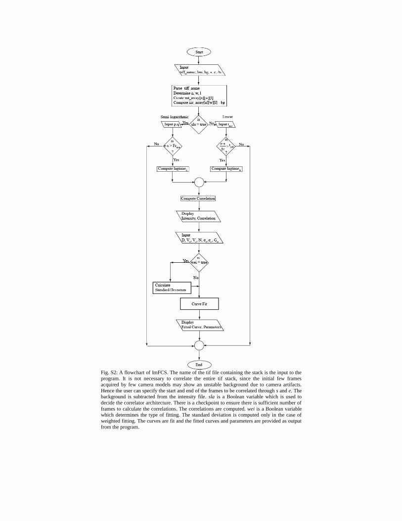
Fig. S2: A flowchart of ImFCS. The name of the tif file containing the stack is the input to the program. It is not necessary to correlate the entire tif stack, since the initial few frames

acquired by few camera models may show an unstable background due to camera artifacts.

Hence the user can specify the start and end of the frames to be correlated through s and e. The background is subtracted from the intensity file. sla is a Boolean variable which is used to

decide the correlator architecture. There is a checkpoint to ensure there is sufficient number of

frames to calculate the correlations. The correlations are computed. wei is a Boolean variable which determines the type of fitting. The standard deviation is computed only in the case of

weighted fitting. The curves are fit and the fitted curves and parameters are provided as output

from the program.

Fig. S3: A screen shot of ImFCS analyzing a diffusion process. The data has been correlated and fitted and quantitative parameters (D, N, χ2) are rendered on the screen.

2. Details of the software

2.1 Software requirements

The function calculating the correlation described above was programmed in C++ using

Microsoft Visual Studio .net 2003(Redmond, WA, USA). This program is controlled using

Igor Pro 6.0 as front end by reprogramming the above program using the external operation

(XOP) tool kit provided by Igor Pro. XOPs were used instead of using Igor procedures

because XOPs in C++ were much faster in performing “number-crunching operations” [1].

The source code is available with the package and the user is free to modify it. If necessary,

the user can include newer fitting models. The program can be adapted for using Igor Pro in

any other operating system or any other front end display software or both. In the former case,

it has to be kept in mind that Igor Pro handles strings differently from many other

programming languages like C, C++ etc since the strings in Igor Pro are not null terminated.

The null character has to be manually added to the name of the tif file while being passed to

the correlation function for calculation.

2.2 Details of the XOP

The XOP serves to transmit the parameters from Igor Pro to the C++ function calculating the

correlations. The parameters which are transferred are the name of the stack file, the binning

value, the minimum value to be subtracted as background, correlator architecture parameters

and the arrays which contain the positions of the pixels to be cross-correlated. The

generalized function calculates the cross-correlation which could be adapted for

autocorrelation as well. The XOP which transfers the name of the tif file to the program is an

adaptation of the example XOP-xstrcat() provided by Igor Pro. In brief, Igor Pro transfers

controls to XOPEntry() function in C++ .net2003 program which in turn transfers the control

to a function which opens the specific tif file for parsing.

2.3 Parsing the tiff file structure

Any tiff file has an “image file header” (IFH) at the beginning. In the program, the IFH is

read to determine the byte order. The byte order is of two types, “little endian” and “big

endian”. The memory in any computer is organized as a series of words. Byte order is the

sequence of storing bits in these words. In the “little endian” configuration, the byte order is

from the least significant bit to the most significant bit and vice versa. The first two bytes in

the IFH indicate byte order. This program works only on “little endian” format and is verified

before execution of the rest of the program. Generally images acquired using Macintosh

operating systems are stored as “big endian” and those from Windows are stored as “little

endian”. Any stack acquired in “big endian” can be converted to “little endian” by open

source image processing software like ImageJ [2].

The IFH contains the magic number [magic number = 42] in the next two bytes.

These two bytes are read and the program continues execution if and only if the value read in

these two bytes is the same as the magic number. The next two bytes indicate the location of

the first “image file directory” (IFD) which locates the first frame in the tiff file.

Each frame is identified by its IFD which determines the location in the file. The

present specification of tiff files allows multiple IFD per tiff file to facilitate the creation of

multi-plane tiff files. Each IFD is an array of values and also contains the location of the

subsequent IFD. The last IFD stores the location of the next IFD as “0” indicating the end of

the stack. The IFDs are read until the value of “0” is reached in order to determine the number

of frames (n) in the particular tiff file. The tags ImageWidth (w) and ImageLength (l) are read

in order to determine the size of each frame. Tiff allows images of different sizes to present in

a single multi-plane tiff file. The software implicitly assumes that the frames in the stack are

of the same dimensions. The n, w and l values are used to define an intensity array which

stores the intensity values of each pixel in the stack of files. This array serves as the input for

the function which calculates the correlation using the intensity values.

The tag BitsPerSample (b) is used in order to determine the amount of bytes

allocated for each pixel in the image. The tag StripOffsets stores the location at which the

intensity values corresponding to the particular IFD is stored. The pointer in the program

assigns w*l*b/8 bytes to a temporary array and w*l values are read beginning from the

position pointed by StripOffsets and stored corresponding to a particular n in the intensity

array. This procedure is repeated for all the frames and the complete intensity array

corresponding to the chosen tiff file is created.

2.4 User Interactive Correlation functions

The software allows the user to draw regions on the average intensity map allowing the user

to select regions where the autocorrelation needs to be performed. This is programmed using

the marquee option in Igor Pro. A marquee is any outline drawn using the mouse on an image.

Getmarquee() function allows one to retrieve the co-ordinates of the vertices of the drawn

outline so that only the pixels within these vertices are correlated. This feature of the software

restricts the user to draw rectangular regions on the graph. The software possesses an

additional option which allows the user to cross-correlate two polygonal shapes on the plot.

The user is provided an option to draw on the average intensity plot for both the regions.

While the user is drawing on the image, all other functions and buttons are disabled. Once the

user finishes the closed polygon (checked by the fact that the user should end the polygon at

the point it was started), the FindPointsinPoly() function is invoked which identifies all the

pixels which are within these two regions. The cross-correlation is calculated and displayed

on the screen. The FindPointsinPoly function invokes the Graphics Device Interface (GDI)

component of the Windows Application Programming Interface’s (API). The GDI contains

the PtInRegion() function which determines whether the pixels lie within the drawn polygon.

2.5 Calculation of the correlation

The summation is implemented using a “nested for loop” with k and l as the counters. The

arrays storing FA and FB are allocated memory dynamically using malloc() for every value of l

since the arrays are reduced in dimension by a factor 2 after every iteration due to the

summing up of adjacent values. The program accepts only even integers for p. In case, the

user enters an odd number, it is incremented by 1.

2.6 Output Parameters

The software provides an average intensity plot as an output. The user has the option to move

the cursor on this plot and display the intensity at any particular pixel in the adjacent window.

Upon correlation, the autocorrelation curve is displayed in an adjacent window. The

autocorrelation and the intensity trace get updated when the cursor is moved in the image plot.

After curve fitting, the fitting parameters are also displayed as images. When the cursor is

moved on any of the above said images, the autocorrelation and intensity traces get updated

and the corresponding fit values along with the pixel position is displayed in the window.

This operation is performed synchronously by monitoring the cursor movement using “hook

functions” described flow.

2.7 Hook functions

The cursor movement is intercepted by a “hook function” which determines the position of

the cursor on the image. Igor Pro manual defines window hook functions as, “A window hook

function is a user‐defined function that receives notifications of events that occur in a specific

window” [1]. The hook function in the software receives information about the movement of

the cursor in the window which displays the average intensity value of the stack. It is

programmed to follow the cursor since it provides the flexibility to the user to use the

keyboard or mouse to move the cursor. The position is transferred to other functions which

move the cursors on other plots to the same position. The corresponding intensity trace and

autocorrelation curve is displayed along with updating the values of fitting parameters

corresponding to the position of the cursor. The entire operation is performed in a

synchronous manner.

2.8 Fitting Algorithm

The user is provided the option of fitting all the pixels in the image or fit only part of them by

choosing a sub-rectangular region in the image. The Levenberg-Marquardt algorithm is used

for non-linear least squares fitting for minimizing the reduced chi-squared2

red [3-6]. The

standard error of the mean or the standard deviation (σi,data) is used for weighting in the

calculation of 2

red . For data, in which σi,data is not available, the program performs

unweighted non-linear least square fitting by assuming the weights to be 1. The major

advantage of using weighted fits is that data points of different precision are handled

differently. If the standard deviation is not the same across the entire set of data points to be

fitted, then weighted least square fitting is beneficial. In a typical correlation curve, the

standard deviation varies with lag time since each point is calculated as an average from a

different number of time points [7]. The fitting is performed without the value of ( 0)G

since this value is affected by the shot noise of the detector. The open source code for the

Levenberg-Marquardt algorithm was available from [8] and was modified to include

weighted least square fitting. The software also provides options to perform fitting by using

the curve fitting tool box in Igor Pro (described in Sec. 7).

The other modification made in the source code was to incorporate conditions in

which the user was provided the flexibility to fix any fitting parameter if necessary. In general,

there may be r fitting parameters in any expression, but from prior knowledge, the user could

have access to some of the values, hence the user has the flexibility to fix the value of k

known fitting parameters and fit the rest r-k parameters. The advantage of using 2

red is that

the value is normalized to the degrees of freedom. Therefore 2

red is close to 1 for a good fit.

2

red > 1 might indicate two things, the model is an inappropriate one to fit the data or it

indicates that the standard error of the mean is underestimated. 2

red < 1 indicates that the

fact that the standard error of the mean is over estimated or the data is overfitted by the model

[9].

2.8.1 Calculating the weight factor

The standard error of the mean (σi,data) can be evaluated in 3 different ways, i) reduced

Koppel’s method, ii) calculation of σi,data while calculating the correlation and iii) by

estimating the standard deviation from the variation of correlations of multiple, non-

overlapping subsets of the data set [7].

Koppel [10] derived an analytical expression for the error in autocorrelation

functions. It has been derived for an exponential signal and it is pointed out by the author that

the expression is “expected to be qualitatively correct for others”. It is to be noted that, since

the expression is derived for an exponential signal, which is a monotonically decreasing

signal, this expression should not be used for cross-correlations which exhibit a peak and

hence are not monotonically decreasing. It has been observed that Koppel’s expression for

standard deviation is a very good approximation of SD at smaller times but fails at longer

times [7, 11, 12]. This led to the development of modified Koppel’s formula. Koppel’s

formula will in general exhibit a minimum, SDmin, at an intermediate lagtime τSD,min and will

then rise with increasing lagtime. This however, is not observed in the data in which the SD is

found to be for τ > τSD,min. Therefore in the modified Koppel’s formula the value of SD is

fixed to SDmin for all τ > τSD,min. In our experience this give 2

red values close to 1. The

expressions for calculations are given in the supplement in Eqs. [S8] and [S9]. In the second

option, the necessary calculations to get an experimental estimate of the SD is performed

alongside the correlations. The formulae to calculate the standard deviation using this method

is given as Eqs. [S10] and [S11] in the supplement.The last method to compute the SD is by

splitting the original intensity file in several non-overlapping stacks for each of which the

correlations are calculated. The SD and standard error for each point in the ACF can then be

calculated from the variation of the multiple correlations.

2.8.2 Comparison of the three methods to determine the correlation

The advantage of using methods other than Koppel’s formula is that they are calculated from

the raw data and are free from any underlying assumptions. But this increases the

computation time as the standard deviation is also calculated while calculating the correlation

mean. In the case of splitting a stack, the number of frames used in calculating individual

correlations to be averaged is reduced by at least a factor of 10. Hence this method is

recommended only if there is sufficiently large number of stacks. Koppel’s method has the

disadvantage that a good estimate of N is necessary since Koppel’s method requires the user

to supply the value of N in the expression. Hence the user has to choose the method based on

the constraints during the calculation.

3. Fitting model

3.1 Fitting model for ITIR-FCCS and IVA-FCCS

Two fitting models are included in the software to fit the data obtained above and to extract

the parameters. The generalized fitting model for cross-correlation for square regions

separated by rx and ry in the x and y axes respectively, for TIRF based camera FCS, for

diffusion and flow processes [13] is given by

2 2 2

2 2 2

2

( - ) ( - ) ( - )2 - - -

4( ) 4( ) 4( )

2 2

2

1( )

4

2- 2

- --2 - ( - )

2 ( ) 2 ( )

-( - )

2 ( )

x x x x x x

df

a r v a r v r v

D D D

x x x x

x x x x

x x

x x

G GNa

De e e

r v a r vr v erf a r v erf

D D

a r va r v erf

D

2 2 2

2 2 2

( - ) ( - ) ( - )2 - - -

4( ) 4( ) 4( )

2 2

2- 2

- --2 - ( - )

2 ( ) 2 ( )

-( - )

y y y y y ya r v a r v r v

D D D

y y y y

y y y y

y

y y

De e e

r v a r vr v erf a r v erf

D D

a ra r v erf

22 ( )

yv

D

[S1]

Here N = <C>a2 where a is the pixel size in object space, C is the surface concentration, τ is

the lagtime, D is diffusion coefficient, vx and vy are the velocities in the x and y axes

respectively and G∞ is the convergence value of the function at long lag times. σ is the

standard deviation of the separable Gaussian approximation to the point spread function (PSF)

of the microscope in the x-y plane [14, 15].

20

2

0 0 0 0

( - )-

20

0

( , , , ) ( , ) ( , )

1( , )

2

x x

em

PSF x x y y PSF x x PSF y y

PSF x x e

where

NA

[S2]

λem is the wavelength of emission and NA is the numerical aperture and σ0 is a numerical

value to be determined by fitting. By setting rx = ry = 0 in Eq. [S1], the model can be

simplified to describe the autocorrelation as in Eq. [S3]. This model has 6 fitting parameters,

D, vx, vy, N, G∞ and σ. It can be seen from Eqn. [S3] that autocorrelation is an even function in

vx and vy. Hence cross-correlations need to be computed to determine the direction of flow.

By setting σ = 0, Eq. [S3] can be simplified into model for autocorrelation as provided in [16,

17].

2 2 2

2 2 2

2

( - ) ( ) ( )2 - - -

4( ) 4( ) 4( )

2

2 2

1( )

4

2- 2

-22 ( )

-( - ) ( )

2 ( ) 2 ( )

x x x

df

a v a v v

D D D

x

x

x x

x x x

G GNa

De e e

vv erf

D

a v a va v erf a v erf

D D

2 2 2

2 2 2

( - ) ( ) ( )2 - - -

4( ) 4( ) 4( )

2

2 2

2- 2

-22 ( )

-( - ) ( )

2 ( ) 2 ( )

y y ya v a v v

D D D

y

y

y y

y y

De e e

vv erf

D

a v a va v erf a v erf

D D

[S3]

3.2 Expressions for ΔCCF for diffusion and flow

The expression for the cross-correlation function for diffusion separated by rx along the x-axis

can be obtained from Eq. [S1] by setting vx = vy = ry = 0 and is an even function in rx. ΔCCF

which is defined as the differences between the forward and the backward correlation, in this

case, is ( , )CCF xG r - ( , )CCF xG r . This expression, evaluates to zero on an average.

2

2

2 2 2

2 2 2

2

( )2 -4( )

2

( ) ( - )2 - - -

4( ) 4( ) 4( )

2

2

1( , )

4

4-1 (2 )

2 ( )

2- 2 - 2

2 ( )

( )2 ( )

x x x

CCF x

a

D

a r a r r

D D D x

x

x

x

G r GNa

D ae a erf

D

rDe e e r erf

D

a ra r erf

D

2

-( - )

2 ( )

x

x

a ra r erf

D

[S4]

This is not the case when the system exhibits flow where the function is not an even function

in rx as seen from the equation below. By setting D = ry = 0, Eq. [S1] is modified as

2

2

2 2 2

2 2 2

( )-

4, 2

( - ) ( - ) ( - )- - -

4 4 4

1 2( ) -1

22

-2- 2 - 2 -

2

- -( - ) ( - )

2 2

x x x x x x

a

CCF f

a r v a r v r v

x x

x x

x x x x

x x x x

aG e a erf

Na

r ve e e r v erf

a r v a r va r v erf a r v erf

[S5]

3.3 Fitting model for SPIM-FCCS

In the case of light sheet of considerable thickness in z direction, the same model was adapted

to include the light sheet thickness and is given in [18].

2 2 2

2 2 2

2

2

( - ) ( - ) ( - )2 - - -

4( ) 4( ) 4( )

2 2

1( )

4 1

2- 2

- --2 - ( - )

2 ( ) 2 ( )

-( - )

x x x x x x

df

z

a r v a r v r v

D D D

x x x x

x x x x

x

x x

G GD

Na

De e e

r v a r vr v erf a r v erf

D D

a r va r v erf

2 2 2

2 2 2

2

( - ) ( - ) ( - )2 - - -

4( ) 4( ) 4( )

2 2

2 ( )

2- 2

- --2 - ( - )

2 ( ) 2 ( )

( -

y y y y y y

x

a r v a r v r v

D D D

y y y y

y y y y

D

De e e

r v a r vr v erf a r v erf

D D

a r

2

-)

2 ( )

y y

y y

a r vv erf

D

[S6]

Where N = 2<C>a2σz where σz is defined as the standard deviation of the Gaussian in the z

direction. It is to be noted that the definitions of N are different in both the expressions. 2

2

( - )-

21( , )

2

z

z m

z

I z m e

[S7]

This model has 4 fitting parameters; D, vx, vy and G∞. The value of σ0 is fixed to 0.61 and the

value of σz can be measured [18]. By a similar reasoning, the cross-correlations have to be

computed to determine the direction in SPIM-FCCS.

4. Standard deviations for weighted fitting

4.1 Koppel’s formula

2

2 2

2

2 2

2

2

g( ) G( ) 1

1 11 2

1

2 11 1  1

| 0

A A

k

g g kkg k

nN g k

g k g k

n NF NF

k k p

[S8]

Subsequently, for the next groups of channels

2 2

2 2

22

2

22

1 2 112

1

2

12 11

 2 1 122 2

2

0, 2

1

l

l

l

l lA A

l

g g yy kg y

n g yN

g y

g y N pwhere y k

n NF F

pk

k l

l q

[S9]

4.2 Calculation of σi,data while calculating the mean

12 21

102 2

0

1 1

0

| 0

n k

A Bn ki

A B

i

n k n

A B

i i k

k

F i F i k

n k F i F i kn k

F i F i

k k p

[S10]

Then, for the groups of channels whose bin widths are in GP, the standard deviation is

evaluated by

221 2 1 1

2 1 122 2

0 22

2

2 1 1

2

2 1 12

22

lll

ll

l

l

l

n p pk i k

i

A B

pi j ij i k

i

l A

j i

pk

F j F j

n pk F j

1

2

2

1 2 1 122 2

02

2

2

2

22

ll

l

l

n p pk i k

B

pij i k

l

A

j i

F j

n pk

F j

1 1 2 1 11 12 22 2 2

0 02

2

0, 2

1

lll l

l

n p n p pk k i k

i

B

pi ij i k

pk

k

F

l

l q

j

[S11]

Fig. S4: This is a representative example of weighted fitting. The original stack was split into 10

smaller stacks. The average and standard deviation of the values were obtained from these 10

datasets.

5. Materials and Methods

5.1 Reagents and Protocols

The lipids used in ITIRFCS measurements were Palmitoyl-2-oleoyl-sn-glycero-3-

phosphocholine (POPC), 1-Palmitoyl-2-Oleoyl-sn-Glycero-3-[Phospho-rac-(1-glycerol)]

(Sodium Salt) (POPG) and 1,2-dipalmitoyl-sn-glycerol-3-phosphoethanolamine-N-(lissamine

rhodamine B sulfonyl) ammonium salt (Rho-PE) obtained from Avanti Polar lipids (Alabaster,

AL). A detailed protocol of the preparation of the lipid bilayers is given in [13]. The details

of the quantum dots, the microscope stage used to demonstrate flow processes are given

elsewhere [13]. IVA-FCS was performed using fluorescent beads (0.17 µm diameter yellow-

green carboxylate modified microspheres λexc = 505 nm, λem= 515 nm, PS SpeckTM

) obtained

from Molecular Probes (Eugene, OR, USA). The preparation of zebrafish embryos and

fluorescent beads for measurement for SPIM-FCS are described in [18]. The growth

condition of CHO cells, the plasmid sequence and the transfection protocols for EGFR-EGFP

are given elsewhere [19].

5.2 Instrumentation

ITIR-FCS and IVA-FCS measurements were performed using an objective-type total internal

reflection fluorescence microscope (TIRFM) built using an inverted epifluorescence

microscope (IX-71, Olympus) with a high NA oil-immersion objective (100X/1.45)

(Olympus, Singapore). Dual color air-cooled ion LASER source (λem = 514 nm, 185-F02,

Spectra-Physics, Mountain View, CA, USA) was used to excite the fluorophores.. The

EMCCD camera (Andor iXON 860, 128x128 pixels) was mounted on the side-port of the

microscope. Andor Solis (Ver: 4.9.30000.0) was used as the image acquisition software. Each

pixel measures 24 x 24 µm2 on the chip and hence a = 240 nm. The measurements were

carried out with a Δτ = 0.56 ms for a ROI of 21 × 21 pixels. The details of the another

instrument used to perform ITIR-FCS are described in [13]. The details of the SPIM-FCS

instrument are provided in [18].

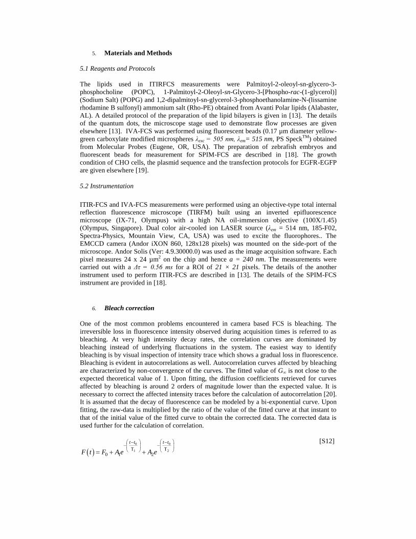
6. Bleach correction

One of the most common problems encountered in camera based FCS is bleaching. The

irreversible loss in fluorescence intensity observed during acquisition times is referred to as

bleaching. At very high intensity decay rates, the correlation curves are dominated by

bleaching instead of underlying fluctuations in the system. The easiest way to identify

bleaching is by visual inspection of intensity trace which shows a gradual loss in fluorescence.

Bleaching is evident in autocorrelations as well. Autocorrelation curves affected by bleaching

are characterized by non-convergence of the curves. The fitted value of G∞ is not close to the

expected theoretical value of 1. Upon fitting, the diffusion coefficients retrieved for curves

affected by bleaching is around 2 orders of magnitude lower than the expected value. It is

necessary to correct the affected intensity traces before the calculation of autocorrelation [20].

It is assumed that the decay of fluorescence can be modeled by a bi-exponential curve. Upon

fitting, the raw-data is multiplied by the ratio of the value of the fitted curve at that instant to

that of the initial value of the fitted curve to obtain the corrected data. The corrected data is

used further for the calculation of correlation.

0 0

1 2

0 1 2

t t t t

F t F A e A e

[S12]

Where F(t) is the decaying fluorescent trace, t0 is the acquisition time of the first frame to be

fitted. T1 and T2 are the fluorescence decay constants. F0, A1, A2, T1 and T2 are fitting

parameters.

7. Curve Fitting in Igor Pro

This program provides an option to the user to perform curve fitting using Igor Pro. It makes

use of FuncFit command in Igor Pro. The FuncFit command provides a variety of options to

check the status of the fit. V_FitQuitReason is a variable defined in Igor which is set to zero

on proper convergence. After the iterations, if V_FitQuitReason equals 0, the fitted parameter

is stored; else it is stored as NAN (Not a Number) indicating a failed fit. The bleach

correction fitting is implemented in Igor Pro.

8. Representative histograms of D and N

Fig.S5: A histogram of the D and N values of the data described in Figs. 2 G-I is shown

in A and B respectively. Fluorescent beads were measured using IVA-FCS in this

example.

9. General guidelines on Imaging FCS measurements

In this section, a few practical guidelines on S/N ratio, pixel size, binning and frame rate of

the camera are provided for the interested users of Imaging FCS.

9.1 S/N ratio

Any data recorded with a camera has a background which is due to the offset of the A/D

converter, the autofluorescence of the sample, the excitation laser leakage and the ambient

light in the room [21]. The background counts needs to be subtracted before the calculation of

the autocorrelation. By experience, we would recommend that the photon counts in the signal

needs to be at least 1.5 times that of the background.

9.2 Photobleaching

The three illumination schemes used for imaging FCS, total internal reflection, variable angle

and single plane illumination, illuminate only those regions in the sample which are being

measured. As a result, there is reduced photobleaching compared to confocal FCS setups. As

a result of reduced phototoxicity, measurements can be performed for longer times, it is also

to be noted that, in SPIM-FCS, the light source is used more effectively and hence SPIM-FCS

can be performed at low laser powers leading to less photobleaching [18].

9.3 Pixel Size and Binning

The pixel size on the object space is determined by the physical size of the pixel and the

magnification of the detection objective. The physical size of the pixel is in turn dependent on

the image capture region size of the chip and the number of pixels in the chip. The optimum

binning to be used for the system depends on the pixel size in the object space. The images

collected on the chip are diffraction limited. Hence, a pixel size smaller than the diffraction

limit, leads only to empty magnification. For cases, where the pixel size is smaller than the

diffraction limit, it can be binned to reach the diffraction limit. A detailed discussion of

binning for ITIR-FCS and SPIM-FCS is available at [13, 16, 18]. It has already been shown

that the diffusion coefficient obtained is independent of the binning used in Imaging FCS [16,

18].

There are two ways to carry out binning, software and hardware binning. The advantage of

using software binning is that, the raw data can be binned to yield greater pixel sizes of any

size by performing the corresponding binning. But, the drawback is that, in the case of

software binning, the binned pixels contains the sum of readout noises of all its constituent

pixels before binning. This drawback is observed in a sCMOS and is not an issue in the case

of EMCCD. In the case of hardware binning, the readout noise is reduced and the data file

occupies less storage space in the memory. While binning, it also has to be kept in mind that,

a binned data has less number of correlations to average and the binning leads to a loss in

spatial resolution.

9.4 Readout Speed of the Camera

The rule of thumb is that measurements need to be about 10 times faster than the fastest

process to be observed by Imaging FCS. The readout speed of the camera is influenced by the

size and shape of the region of interest. Reading a sub-array of the chip of the camera

increases the readout of the camera. Presently, we have measured up to 2000 fps on a square

region of 20 pixels. A lipid bilayer was prepared and the same sample was measured for a

wide variety of readout speeds from 250 to 2000 fps and there was only a 10% change in D’s

extracted from these datasets [data not shown]. A 1 way ANOVA revealed that the

differences between D obtained at frame rates of 250, 500 and 1000 are not statistically

significant at the 0.2% level. It should also be remembered that data collected using faster

frame rates are noisier than those collected with slower frame rates. In the case of a lipid

bilayer, the standard deviation of the D’s is 50% of the mean value in the case of 2000 fps,

whereas the standard deviation of the D’s are 30% of the mean at slower frame rates (250-

1000 fps).

10. Comparison of Imaging FCS with other fluorescent methods

ITIR-FCS has been systematically compared with other fluorescent techniques like

Fluorescent Recovery After Photobleaching (FRAP), confocal FCS and Single Particle

Tracking (SPT) in [16]. In general, the diffusion coefficients obtained from ITIR-FCS are

comparable with those obtained from FRAP. The Ds obtained from confocal FCS are larger

than those from ITIR-FCS. This is due to the limited time resolution of the state of the art

cameras today. SPT shows a wider range of D’s when compared to that of ITIR-FCS. Using

z-scan FCS or two-focus (2f) FCS, both of which are calibration free methods, the diffusion

coefficients of lipids diffusing on a bilayer was determined to be 2–5 µm2/s [22-24]. The

values obtained from ITIR-FCS also fall in the same range [13]. In the case of measurements

on biological systems, it was demonstrated using ITIR-FCS that there is a 2-3 times increase

in D of raft markers upon treatment with cholesterol depleting or/and actin depolymerizing

agents. The same trend has been observed by other techniques as well. Image Correlation

Spectroscopy revealed that upon cholesterol depletion, D increased by a factor of 2 for GPI

anchored proteins [25]. Using FRAP, it was demonstrated that cholesterol removal or

cytoskeletal disruption led to a 2-3 times increase in increase in D for Dopamine transporter

protein [26]. The accuracy of the D’s extracted out of SPIM-FCS were demonstrated by the

authors using different experiments on fluorescent beads [18]. In the case of IVA-FCS, the

diffusion coefficient of beads reported here, the values are similar to those obtained from

SPIM-FCS [18]. In conclusion, all the Imaging FCS methods retrieve diffusion coefficients

which are comparable with expected values and those obtained from other techniques.