Supplementary Appendix for - Cambridge University Press

Supplementary Appendix for:de la Cuesta, Brandon, Naoki Egami, and Kosuke Imai.

“Improving the External Validity of Conjoint Analysis: TheEssential Role of Profile Distribution.” Political Analysis

A Review of Conjoint Literature

A review of the literature was conducted to assess several features of current best practices.

In order to gather a sufficiently large number of articles, we selected 10 journals for a key-

word search (“conjoint”): The American Journal of Political Science, The American Political

Science Review, The British Journal of Political Science, Journal of Experimental Political

Science, Journal of Politics, Political Analysis, Political Behavior, Political Science Research

and Methods, Research and Politics, and the Review of International Organizations. This

search criteria resulted in a total of 40 articles. We then augmented this list by examining

articles that cited Hainmueller et al. (2014) using Google’s “cited by” feature to obtain arti-

cles from additional journals or articles from the list above that were missed in the keyword

search. This resulted in an additional 25 articles. We removed from the list any article whose

contribution was primarily or completely methodological. This procedure left us with a total

of 59 articles from 2014 to 2019. This list is not meant to be exhaustive but rather to be broad

enough to give an overview of current practice.

Each article was then examined and classified along several dimensions. First, we coded

the randomization distribution used in the design, characterizing each article by the number

of factors used in the fielded design and the number that were randomized according to the

uniform. In many cases, authors made no mention of the exact randomization probabilities or

simply noted that their designs were “fully randomized”. In cases where there was ambiguity

about the distribution used, we consulted the appendix material to determine the distribu-

tion. If the appendix did not contain information sufficient to determine the distribution, we

examined the uniformity of the standard errors of reported estimates and counted a factor as

being randomized according to the uniform if the standard errors of all of that factor’s levels

were indistinguishable from each other.

We then examined the main text to establish whether the authors justified the distribution

they chose on theoretical grounds. Justifications that would yield an affirmative coding include

explicit discussion of the desire to match population distributions or the desire for statistical

efficiency. An affirmative coding was given even if the discussion was relegated to a footnote

and concerned only a single factor. Discussion of the constraints placed on unrealistic factor

combinations was not part of the criteria used. As such, some papers that use such constraints

were nonetheless considered as not invoking a substantive or theoretical justification for their

chosen distribution.

Finally, for each paper we examined all factors that were a part of the design and de-

1

termined whether it was feasible to collect data that would allow the approximation of the

population distribution for that factor. Designs in which population data could be feasibly

collected for most or all factors were considered to be amenable to the use of population data

in the design or analysis stage. The articles are given below in Table A1 .

Author Year Title

Atkeson and Hamel 2018 Fit for the job: candidate qualifications and vote choice in lowinformation elections

Auerbach and Thachil 2018 How clients select brokers: competition and choice in India’s slums

Ballard-Rosa et al 2017 The structure of American income tax policy preferences

Bansak et al 2016 How economic, humanitarian, and religious concerns shape Euro-pean attitudes toward asylum seekers

Bechtel and Scheve 2013 Mass support for global climate agreements depends on institu-tional design

Bechtel et al 2017 Interests, norms and support for the provision of global publicgoods: The case of climate co-operation

Bechtel et al 2017 Policy design and domestic support for international bailouts

Berinksy et al 2018 Attribute affinity: U.S. natives’ attitudes towards immigrants

Bernauer et al 2019 Do citizens evaluate international cooperation based on informa-tion about procedural and outcome equality?

Breitensten 2019 Choosing the crook: a conjoint experiment on voting for corruptpoliticians

Bueno 2017 Bypassing the enemy: distributive politics, credit claiming, andnonstate organizations in Brazil

Campbell et al 2016 Legislator dissent as a valence signal

Carnes and Lupu 2016 Do voters dislike working-class candidates? Voter biases and thedescriptive underrepresentation of the working class

Chauchard 2016 Unpacking ethnic preferences: theory and micro-Level evidencefrom north India

Chilton et al 2017 Reciprocity and public opposition to foreign direct investment

Clayton et al 2019 Exposure to immigration and admission preferences: evidencefrom France

Crowder-Meyer et al 2018 A different kind of disadvantage: candidate race, cognitive com-plexity, and voter choice

Eggers et al 2017 Corruption, accountability and gender: do female politicians facehigher standards in public life

Franchino and Segatti 2019 Public opinion on the Eurozone fiscal union: evidence from surveyexperiments in Italy

Franchino and Zucchini 2014 Voting in a multidimensional space: a conjoint analysis employingvalence and ideology attributes of candidates

2

Gallego and Marx 2016 Multi-dimensional preferences for labour market reforms

Goggin et al 2019 What goes with red and blue? Mapping partisan and ideologicalassociations in the minds of voters

Hainmueller and Hopkins 2015 The hidden American immigration consensus: a conjoint analysisof attitudes towards immigrants

Hainmueller et al 2015 Validating vignette and conjoint survey experiments against real-world behavior

Hankinson 2018 When do renters behave like homeowners? High rent, price, anxi-ety, and NIMBYism

Hartman and Morse 2018 Violence, empathy and altruism: evidence from the Ivorian refugeecrisis in Liberia

Hausermann et al 2019 The politics of trade-offs: studying the dynamics of welfare statereform with conjoint experiments

Heinric and Kobayashi 2017 Sanction consequences and citizen support: a survey experiment

Heinric and Kobayashi 2018 How do people evaluate foreign aid to ‘nasty’ regimes?

Hemker and Rink 2017 Multiple dimensions of bureaucratic discrimination: evidence fromGerman welfare offices

Horiuchi et al 2018 Measuring voters’ multidimensional policy preferences with con-joint analysis: application to Japan’s 2014 election

Horiuchi et al 2018 Identifying voter preferences for politicians’ personal attributes: aconjoint experiment in Japan

Huff and Kertzer 2017 How the public defines terrorism

Iyengar and Westood 2015 Fear and loathing across party lines: new evidence on group po-larization

Karpowitz et al 2017 How to elect more women: gender and candidate success in a fieldexperiment

Kertzer et al 2019 How do observers assess resolve?

Kirkland, Coppock 2018 Candidate choice without party labels

Leeper, Robison 2018 More important, but for what exactly? The insignificant role ofsubjective issue importance in vote decisions

Li and Zeng 2017 Individual preferences for FDI in developing countries: experimen-tal evidence from China

Liu 2018 The logic of authoritarian political selection: evidence from a con-joint experiment in China

Malhotra and Newman 2019 Explaining immigration preferences: disentangling skill and preva-lence

Mares and Visconti 2019 Voting for the lesser evil: evidence from a conjoint experiment inRomania

Mummolo 2016 News from the other side: how topic relevance limits the preva-lence of partisan selective exposure

Mummolo and Nall 2016 Why partisans do not sort: the constraints on political segregation

3

Newman and Malhotra 2018 Economic reasoning with a racial hue: is the immigration consen-sus purely race neutral?

Oliveros and Schuster 2018 Merit, tenure, and bureaucratic behavior: evidence from a conjointexperiment in the Dominican Republic

Ono and Burden 2018 The contingent effects of candidate sex on voter choice

Ono and Yamada 2018 Do voters prefer gender stereotypic candidates? Evidence from aconjoint survey experiment in Japan

Peterson 2017 The role of the information environment in partisan voting

Peterson and Simonovitis 2018 The electoral consequences of issue frames

Sances 2018 Ideology and vote choice in U.S. mayoral elections: evidence fromFacebook surveys

Scheider 2019 Euroscepticism and government accountability in the EuropeanUnion

Sen 2017 How political signals affect public support for judicial nominations:evidence from a conjoint experiment

Shafranek 2019 Political considerations in nonpolitical decisions: a conjoint anal-ysis of roommate choice

Spilker et al 2016 Selecting partner countries for preferential trade agreements: ex-perimental evidence from Costa Rica, Nicaragua, and Vietnam

Teele et al 2018 The ties that double bind: social roles and women’s underrepre-sentation in politics

Vivyan and Wagner 2016 House or home? Constituent preferences over legislator effort al-location

Ward 2019 Public attitudes towards young immigrant men

Write et al 2016 Mass opinion and immigration policy in the United States: re-assessing clientelist and elitist perspectives

Table A1: Conjoint Articles Published From 2014-2019.

B Constructing the Target Profile Distribution

We utilize several sources of data to construct the population distribution used in Section 2. We

emphasize that ideally researchers should construct the population profile distribution before

designing conjoint analysis in order to match the attributes of the population distribution

with those of conjoint analysis. In the current application, we construct the population profile

distribution after the conjoint analysis was conducted by Ono and Burden (2019). As a result,

for almost all factors, additional ex post coding was needed to match the empirical data to the

categories chosen by the original authors.

Here, we discuss the data source and the procedure used to produce categories matching

those used in the original experiment. We use the legislators in the 115th Congress as the

4

Factors Levels Population Data Source

Age 36, 44, 52, 60, 68, 76 Daily Kos Biographical Database

Gender Male, Female

Race Asian, Black, Hispanic, White

Family Divorced, Never married, Married(no children) Married (2 children)

The Hill People Directory

Experience None, 4 years, 8 years, 12 years Daily Kos Biographical Database

Expertise Economic policy, Education, En-vironmental issues, Foreign policy,Health care, Public safety (crime)

Congressional Committee Assign-ments

Character Trait Compassionate, Honest, Intelligent,Knowledgeable, Leadership, Empa-thetic

None

Immigration Policy Favors guest worker program, op-poses guest worker program

Secure America’s Future Act(SAFA) Roll Call Votes

Security Policy Strong military, Cut defense spend-ing

Center for Security Policy LegislatorScorecard

Abortion Policy Pro-choice, Neutral, Pro-life National Right to Life Council Leg-islator Scorecard

Deficit Policy Increase taxes, Take no action, Re-duce spending

Club for Growth Legislator Score-card

Table A2: Levels and Data Sources Used to Construct the Population Profile Distribution.

target population distribution in order to maximize our ability to reverse engineer the original

factor levels. To merge disparate data sources, we use a probabilistic record linkage method,

implemented via the R package fastLink (Enamorado et al., 2019), with partial matching on

the first and last name. Table A2 lists the data source used to build the empirical distribution

for each factor. In calculating these factors, we considered only legislators who were seated

via popular vote; those who were named to a seat due to a vacancy are omitted.

B.1 Demographic Factors

Age, gender and race — the three demographic factors used in the original study — were

obtained from the Daily Kos 115th Congress Members Guide. The dataset contains both

biographical and electoral information. Biographical information on legislators is sourced from

Pew, Roll Call, news stories and Wikipedia. Data was also checked against a similar dataset

available through legislatoR (Gobel and Munzert, 2019), an R package that allows queries

to a database of biographical and political information on legislators from multiple countries.

The details about each demographic factor is presented below.

5

Age. The age factor was produced by binning legislators’ ages into the same age ranges as

the original categories.

Gender. Legislator gender was taken directly from the data and unaltered.

Race. Racial categories closely matched those of the experiment with some notable excep-

tions. First, legislators that were coded as identifying as both white and Hispanic were coded

as Hispanic in the joint data. Two legislators who identified as white-Portuguese American

were coded as White. All Asian-American legislators were coded as Asian-American regardless

of their nationality. For example, an Indian-American and Japanese American legislator would

both be coded as Asian-American.

B.2 Background Factors

Background factors were constructed from four sources: the Daily Kos 115th Congress Mem-

bers Guide, legislators’ official Wikipedia page; the Congressional Committees dataset (Stewart

and Woon, 2017); and biographical information from the People directory of TheHill.com, a

digital news site.

Experience. The experience measure was created by first subtracting the first year a leg-

islator was elected to higher office from the most recent election year, resulting in a measure

of the total number of years spent in office. To calculate years served, the election year for

all House members was taken as 2016—the year of the most recent House elections present in

the data—while for Senators the election year in which they won current office was used. If a

legislator had served previously, this interval was added to the more recent tenure. In a limited

number of cases, a legislator was seated as a result of a special election. In these cases, the

year of the special election is used. To map this measure onto the categories of the factor used

in the original experiment (0 years, 4 years, 8 years, 12 years), we use the midpoints between

each category to determine into which bin each observation falls. For example, a legislator

with 1 year experience would fall to the left of the midpoint between the two nearest categories

(0 and 4 years, respectively) and be assigned to the 0 years category.

Policy Expertise. The policy expertise factor is difficult to approximate with real-world

data because the expertise that legislators claim during campaigns may be a matter of political

expedience and may not correspond to their actual expertise. To overcome this difficulty, we

used legislators’ committee assignments as the basis for producing the joint distribution. Our

motivation for using committee assignments is straightforward: legislators are strategic in

their choice of committee assignments—or at least in their attempts to obtain assignments

that would allow them to claim expertise in politically salient areas. Using the Congressional

Committees dataset, we attempted to map each committee—in both the House and Senate—

to a corresponding category in the original experiment. Where the committee was a poor

match for all of the original categories, such as for the Ways and Means Committee, we coded

a legislator’s expertise as missing.

6

http://web.mit.edu/17.251/www/data_page.html#2

https://thehill.com/people

Because each legislator serves on multiple committees and our joint distribution is con-

structed at the legislator-level, there are multiple values possible for each legislator. To over-

come this problem, for each legislator we compared the seniority rankings of each committee

and assigned to that legislator the committee on which they were the most senior. Because

not all committees are the same size, it is possible that a legislator could be assigned a small

committee in which they were a higher rank in absolute terms but lower as a percentage of

total seats. We allow for such cases because a high absolute ranking on a small committee may

be used as the basis for a claim of expertise as easily as a lower ranking in a larger committee.

Party. Party was taken directly from the Daily Kos dataset and then binned into three

categories: Democrat, Republican and Independent.

Favorability Rating. Because we were interested in a large pool of legislators, it was not

possible to obtain favorability ratings drawn from a sufficiently large survey sample for the

majority of our legislators. To overcome this, we used the vote margin in the previous election

as a proxy for legislators’ approval ratings in their constituency. Due to the mechanics of first-

past-the-post elections, this means that the lowest level of favorability rating possible in the

experiment (34%) occurs only twice and the next highest rating (43%) occurs only six times.

This right-skewed distribution is a good approximation of the true favorability rating for two

reasons. First, viable candidates in competitive districts must have reasonably high approval

ratings with the general electorate. Second, legislators in stronghold districts are likely to have

high approval ratings due to their copartisanship with the majority of their constituents.

Family Status. The original “family” factor included information on marital status and

legislators’ number of children. Data on both were harvested from legislators’ Wikipedia

pages using the rvest package in R (Wickham, 2019) wherever such fields were available.

Because legislators may not wish to publicize that they are divorced or unmarried, it is possible

that missingness is correlated with legislators’ marital status. We attempted to address this

problem by augmenting the Wikipedia data with data harvested from the People Directory

of TheHill.com. For both the Wikipedia and TheHill.com fields, the names of spouses and

number of children were given. In the case of multiple marriages, we coded legislators’ marital

status based on the status of their most recent marriage. Thus, a legislator who is currently

married but was divorced in the past would be coded as married. To use this data to re-

construct the categories used in the conjoint experiment, it was necessary to bin the number

of children into the original categories. Legislators with 1 or more children were binned into the

“2 children” category. The number of children was disregarded if the legislator was divorced

or never married because the original categories contained no information on the number of

children for those marital statuses. Legislators for whom the number of children field was

missing in both TheHill and Wikipedia datasets were coded as having zero children.

7

B.3 Policy Positions

The original data contained information on four policy dimensions: abortion (pro-life/pro-

choice/neutral); immigration (in favor of/against a guest worker program); security (favors

strong military/favors defense spending cuts); and deficit reduction (wants to reduce deficit

through tax increases/wants to maintain current deficit/wants to reduce deficit through spend-

ing cuts). These factors were difficult to approximate with real-world data for several reasons.

First, they correspond to broad issue areas, such as a legislators’ stance on abortion. In such

cases, real-world legislators’ policy positions are likely to be driven by one or more latent di-

mensions that can only be estimated from voting behavior across many bills. Second, estimates

of this latent dimension via voting behavior are complicated by the fact that we are restricted

to considering only bills introduced in and voted on during the 115th Congress, resulting in

relatively few bills that correspond to the original levels. Third, for positions that are subsets

of a broader policy space—such as the desired means of deficit reduction—a bill with a pro-

posal similar to the original levels will often include statutes related to other, similar issues.

Special care thus needs to be taken to ensure that legislators’ voting behavior was driven at

least in part by the statute corresponding to the original levels.

Finally, while policy think tanks often provide legislator scorecards, the score space may not

correspond neatly to the levels of the original data. For example, someone who is considered

moderate on fiscal issues may not necessarily advocate for no deficit reduction, which is the

middle category of the spending policy factor. Given these considerations, we aimed to build a

reasonable first approximation using a combination of actual voting behavior. In cases where

legislators’ voting behavior was not available or driven by other statutes included in a bill,

legislator scorecards produced by advocacy organizations and partisan policy institutes were

consulted.

To facilitate consistency across the four policy factors in the original data, we used a

general heuristic in deciding whether to use a bill or a legislator scorecard to approximate the

experimental categories. We began by identifying legislative scorecards whose policy space

closely matched the policy referenced in the original factor. If none were available, a scorecard

for a more broad issue area could also be used.

Legislator scorecards are typically constructed by “scoring” legislators’ votes on bills that

are considered important in a particular policy space. The think tank producing the scorecard

then rates each legislator according to how closely their voting behavior matches the position

favored or advocated by the organization. While such scorecards are available from both

conservative and liberal policy institutes, we chose only from scorecards issued by conservative

organizations. This was done to ensure that a higher score was always associated with a more

conservative policy position. Once the scorecard was obtained, we examined the bills used to

produce each legislators’ score. If a bill closely matched the original categories and was voted

on in the 115th Congress, each legislators’ vote was used to assign him or her a policy position.

8

To ensure that the policy position distribution was not driven by only a few legislators, bills

meeting these criteria were only used if they were considered in both the House and Senate in

similar form or the House alone.

If there existed no bill that was suitable for approximating actual legislators’ values on the

original factor, the legislator scorecards were used directly. To do so, legislators were binned

into categories according to their numerical score and normalized to range from 0 to 1. A

score of 1 was given to legislators considered strong proponents of a given policy position. If

the original factor had only two categories — as in the case of the national security factor,

for example — legislators with a value at or below the midpoint (a score of 0.5) were given

the value corresponding to the liberal position, while those above were assigned to the more

conservative category. In cases where the original factor had three categories, legislators with

scores from 0 to 0.4 were given the liberal position, those with scores between 0.4 and 0.6 were

given the moderate position, and those at 0.6 or above were given the conservative position.

Given these decision rules, we selected legislator scorecards for the abortion, deficit spend-

ing and national security factors and a single bill for the immigration factor. Below we describe

the data source and coding rules used to produce categories matching those of the original

study.

Abortion. Data for abortion position was based on the National Right to Life Council

(NRLC) legislator scorecard. While the NRLC is a conservative, pro-life organization, similar

scorecards from left-leaning organizations produce similar distributions owing to the highly

polarized nature of abortion policy in the United States. The NRLC score is a 0-1, with

1 corresponding to a strongly pro-life legislator and a zero a strongly pro-choice legislator.

Legislators between 0 and 0.4 were coded as pro-choice; those between 0.4 and 0.6 were coded

as neutral; and those with a score greater than 0.6 were coded as pro-life. Predictably, there

are only three neutral legislators according to this criteria, and the distribution is almost

perfectly correlated with partisanship.

Immigration. Using the decision rules above, we chose a bill rather than a legislator score-

card, selecting the Secure America’s Future Act (SAFA) to serve as our proxy for legislators’

positions on the guest worker program. SAFA included in it a provision to abolish the existing

H-2B guest worker program with a less generous and more restricted policy dubbed H-2C.

While other provisions of the bill were politically important—such as protection for so-called

Dreamers—the guest worker program was a prominent feature of the bill. This is the only case

for the 115th Congress where an immigration bill including a program closely corresponding

to the Ono and Burden levels was both introduced and voted on. Because a vote in favor

of SAFA was a vote for the H-2C guest worker program (and thus against the existing H-2B

system), a vote of yes was coded as opposition to a guest worker program and a vote of no as

favoring a guest worker system. Legislators who did not vote were marked as missing.

9

National Security. Data for the military spending factor was based on the Center for

Security Policy (CfSP) legislator scorecard. The CfSP scored a total of 19 bills to produce a

0-1 score where higher values represents more “pro-security” voting behavior. Legislators with

a score less than 0.5 were binned into the “cut military spending” category while those above

the cutoff were binned into the “maintain strong defense” category.

Budget. Data for the budget position was based on the Club for Growth’s legislator score-

card. The Club for Growth, a conservative organization, rated legislators according to the

organization’s pro-deficit-reduction position, producing a scorecard with a range of 0-1 where

higher values indicate more support for deficit reduction. Legislators with a score between 0

and 0.4 were given a value of “reduce deficit through tax increases”, a liberal position; those

with a score between 0.4 and 0.6 were given the moderate position “do not reduce deficit now”;

and those with a score greater than 0.6 were given the conservative position “reduce deficit

through spending cuts”.

C Robustness to the Choice of Profile Distribution

The original experiment design of Ono and Burden (2019) considers hypothetical political can-

didates. Thus, the ideal target profile distribution would be the real-world distribution of the

attributes summarized in Table 1 for all candidates, not only sitting legislators. Unfortunately,

because the original experiment was not designed with fidelity to the real-world distribution

in mind, there are many factors for which it is practically impossible to gather corresponding

real-world distributions of all candidates (e.g., character traits of candidates and favorability

rating). As a result, in Section 3.4.1, we set our main target profile distribution to be politi-

cians in the 115th Congress, for whom we were able to collect real-world distributions for most

factors (as described in detail in Section B).

In this section, we use the model-based approach to investigate the robustness of the

pAMCE estimates based on the 115th Congress (reported in Section 5.1) to alternative profile

distributions based on candidate-level data. Although these candidate-level data do not include

information for all factors used in the original experiment, we can incorporate a number of

relevant candidates’ characteristics. In particular, we rely on two publicly available datasets

on candidate characteristics, DIME data set (Bonica, 2015) and the Reflective Democracy

(RefDem) dataset,9 to improve the profile distributions of three demographic variables. In

addition, we use our substantive knowledge to explore different theoretically relevant profile

distributions on policy dimensions.

Data. For the DIME data (Bonica, 2015), we consider all major party candidates that ran

for Congress in the 2014 general election, the last year of the dataset’s coverage. This yields

1148 candidates. In the RefDem data, we consider all major party candidates who ran for

the House or Senate in 2018. This yields 911 unique candidates. We use the DIME data to

9This dataset is available at https://wholeads.us/resources/for-researchers/

10

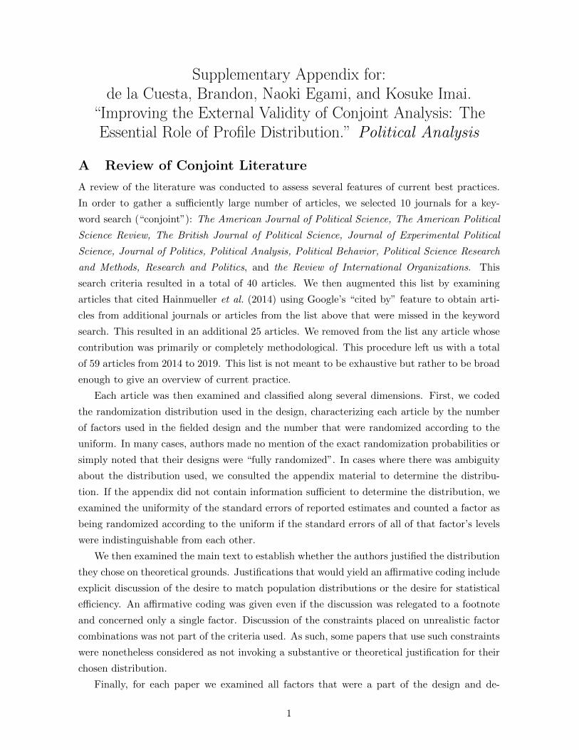
https://wholeads.us/resources/for-researchers/

replace the marginal distribution for number of years in office (Experience), and the RefDem

data to replace the marginal distributions of race and gender (Race, Gender). Figure A1

visualizes this new distribution. Comparing to Figure 2, the two most notable differences are

the larger proportion of white candidates — particularly for Democrats — and the higher inci-

dence of candidates with “no experience,” a natural consequence of considering challengers. In

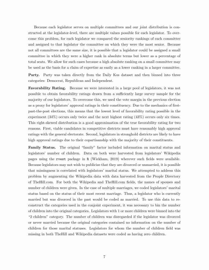
a second profile distribution, we also augment these new demographic marginal distributions

with changes to the marginal distributions of policy positions, making them more extreme to

reflect the fact that winning candidates are systematically more moderate than losing candi-

dates. Figure A2 visualizes this second new distribution. On all policy dimensions, we made

the policy positions slightly more extreme, and it can be clearly seen in positions on Deficit.

Our goal is to assess the robustness of the pAMCE based on the 115th Congress to these

alternative target profile distributions.

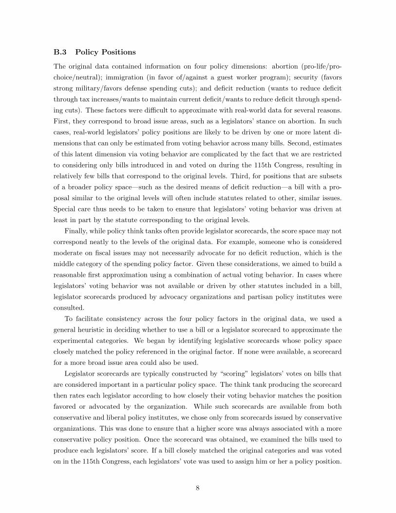
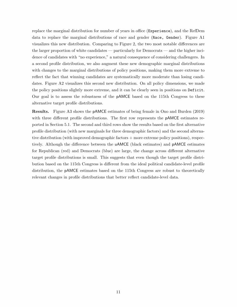
Results. Figure A3 shows the pAMCE estimates of being female in Ono and Burden (2019)

with three different profile distributions. The first row represents the pAMCE estimates re-

ported in Section 5.1. The second and third rows show the results based on the first alternative

profile distribution (with new marginals for three demographic factors) and the second alterna-

tive distribution (with improved demographic factors + more extreme policy positions), respec-

tively. Although the difference between the uAMCE (black estimates) and pAMCE estimates

for Republican (red) and Democrats (blue) are large, the change across different alternative

target profile distributions is small. This suggests that even though the target profile distri-

bution based on the 115th Congress is different from the ideal political candidate-level profile

distribution, the pAMCE estimates based on the 115th Congress are robust to theoretically

relevant changes in profile distributions that better reflect candidate-level data.

11

0.0

0.2

0.4

0.6

0.8

1.0

Pro

babi

lity

Male

Fem

aleW

hite

Hispan

ic

Asian

Amer

ican

Black

36 ye

ars o

ld

44 ye

ars o

ld

52 ye

ars o

ld

60 ye

ars o

ld

68 ye

ars o

ld

76 ye

ars o

ld

Single

(nev

er m

arrie

d)

Single

(divo

rced

)

Mar

ried

(no

child

)

Mar

ried

(two

child

ren)

None

4 ye

ars

8 ye

ars

12 ye

ars

Econo

mic

polic

y

Educa

tion

Enviro

nmen

tal is

sues

Fore

ign p

olicy

Health

care

Public

safet

y (cr

ime)

Gender Race Age Family Experience Expertise

UniformRepublicanDemocrat

0.0

0.2

0.4

0.6

0.8

1.0

Pro

babi

lity

Compa

ssion

ate

Hones

t

Inte

lligen

t

Knowled

geab

le

Provid

es st

rong

lead

ersh

ip

Really

care

s abo

ut p

eople

like

you

Favo

rs g

iving

gue

st wor

ker s

tatu

s

Oppos

es g

iving

gue

st wor

ker s

tatu

s

Cut m

ilitar

y bud

get

Main

tain

stron

g de

fense

Pro−c

hoice

No op

inion

(neu

tral)

Pro−li

fe

Reduc

e de

ficit t

hrou

gh ta

x inc

reas

e

Don't r

educ

e de

ficit n

ow

Reduc

e de

ficit t

hrou

gh sp

endin

g cu

ts34

%43

%52

%61

%70

%

Trait Security Abortion Deficit FavorabilityImmigration


Figure A1: Experimental and Target Profile Distributions of Factors in Ono and Burden (2019)improved by candidate-level data sets.

12

0.0

0.2

0.4

0.6

0.8

1.0

Pro

babi

lity

Male

Fem

aleW

hite

Hispan

ic

Asian

Amer

ican

Black

36 ye

ars o

ld

44 ye

ars o

ld

52 ye

ars o

ld

60 ye

ars o

ld

68 ye

ars o

ld

76 ye

ars o

ld

Single

(nev

er m

arrie

d)

Single

(divo

rced

)

Mar

ried

(no

child

)

Mar

ried

(two

child

ren)

None

4 ye

ars

8 ye

ars

12 ye

ars

Econo

mic

polic

y

Educa

tion

Enviro

nmen

tal is

sues

Fore

ign p

olicy

Health

care

Public

safet

y (cr

ime)

Gender Race Age Family Experience Expertise


0.0

0.2

0.4

0.6

0.8

1.0

Pro

babi

lity

Compa

ssion

ate

Hones

t

Inte

lligen

t

Knowled

geab

le

Provid

es st

rong

lead

ersh

ip

Really

care

s abo

ut p

eople

like

you

Favo

rs g

iving

gue

st wor

ker s

tatu

s

Oppos

es g

iving

gue

st wor

ker s

tatu

s

Cut m

ilitar

y bud

get

Main

tain

stron

g de

fense

Pro−c

hoice

No op

inion

(neu

tral)

Pro−li

fe

Reduc

e de

ficit t

hrou

gh ta

x inc

reas

e

Don't r

educ

e de

ficit n

ow

Reduc

e de

ficit t

hrou

gh sp

endin

g cu

ts34

%43

%52

%61

%70

%

Trait Security Abortion Deficit FavorabilityImmigration


Figure A2: Experimental and Target Profile Distributions of Factors in Ono and Burden (2019)improved by candidate-level data sets and augmented with counterfactual more extreme policypositions.

13

●

●

●

−0.10 −0.05 0.00 0.05 0.10

Congressional Candidates

Estimates

●

●

●Uniform

Republican

Democrat

115t

h C

ongr

ess

●

●

●

−0.10 −0.05 0.00 0.05 0.10Estimates

●

●

●

Adj

uste

d by

Can

dida

te−l

evel

dat

a

●

●

●

−0.10 −0.05 0.00 0.05 0.10Estimates

●

●

●

Adj

uste

d by

Can

dida

te−l

evel

dat

a +

Mor

e ex

trem

e po

licy

posi

tions

●

●

●

−0.10 −0.05 0.00 0.05 0.10

Presidential Candidates

Estimates

●

●

●

●

●

●

−0.10 −0.05 0.00 0.05 0.10Estimates

●

●

●

●

●

●

−0.10 −0.05 0.00 0.05 0.10Estimates

●

●

●

Figure A3: Estimates of the pAMCEs of Being Female in Ono and Burden (2019) with threedifferent profile distributions. The first row represents the pAMCE estimates reported inSection 5.1. The second and third rows show results based on the first alternative profiledistribution (with improved three demographic variables) and the second alternative profiledistribution (with improved three demographic variables + more extreme policy positions).

14

D Proofs

D.1 Consistency of Weighted Difference-in-Means

Here, we formally prove that the proposed weighted difference-in-means estimator is consistent

for the pAMCE under any randomization distribution that satisfies a set of positivity conditions.

Theorem 1 (Consistency of the Weighted Difference-in-Means Estimator) The weighteddifference-in-means estimator defined in equation (5) is consistent for the pAMCE,

pτ�` pt1, t0q pÝÑ τ�` pt1, t0q, (A1)

for any randomization distribution PrRp�q that satisfies the following positivity conditions,

PrRpTijk` � t1 | pTijk,�`,Ti,�j,kq � tq ¡ 0

PrRpTijk` � t0 | pTijk,�`,Ti,�j,kq � tq ¡ 0

PrRppTijk,�`,Ti,�j,kq � tq ¡ 0

for all t P T � where T � is the support of Pr�pTijk,�`,Ti,�j,kq.

The positivity requirement guarantees that all possible profile combinations under the target

population distribution have non-zero probabilities under the randomization distribution. The

proposed three designs satisfy this requirement.

Proof. We want to prove that the following estimator is consistent for the pAMCE.

pτ�` pt1, t0q �

°Ni�1

°Jj�1

°Kk�1 1tTijk` � t1uwijk`Yijk°N

i�1

°Jj�1

°Kk�1 1tTijk` � t1uwijk`

�

°Ni�1

°Jj�1

°Kk�1 1tTijk` � t0uwijk`Yijk°N

i�1

°Jj�1

°Kk�1 1tTijk` � t0uwijk`

,

where the weights are defined as,

wijk` �1

PrRpTijk` | Tijk,�`,Ti,�j,kq�

Pr�pTijk,�`,Ti,�j,kq

PrRpTijk,�`,Ti,�j,kq.

We first focus on the numerator. By the law of large number, we can obtain

1

NK

N

i�1

K

k�1

1tTijk` � t1uwijk`YijkpÝÑ ErERr1tTijk` � t1uwijk`Yijkss,

where the first expectation is over a random sample of respondents i and task positions k,

and the second expectation is over randomization of treatment assignment. We focus on the

expression inside the first expectation.

ERr1tTijk` � t1uwijk`Yijks�

¸ptijk,�`,ti,�j,kq

ERr1tTijk` � t1uwijk`Yijk | Tijk,�` � tijk,�`,Ti,�j,k � ti,�j,ksPrRpTijk,�` � tijk,�`,Ti,�j,k � ti,�j,kq

�¸

ptijk,�`,ti,�j,kq

ERr1tTijk` � t1uwijk`YijkpTijk` � t1,Tijk,�` � tijk,�`,Ti,�j,k � ti,�j,kq | Tijk,�` � tijk,�`,Ti,�j,k � ti,�j,ks

�PrRpTijk,�` � tijk,�`,Ti,�j,k � ti,�j,kq(

�¸


tYijkpTijk` � t1,Tijk,�` � tijk,�`,Ti,�j,k � ti,�j,kqwijk`

15

�ERr1tTijk` � t1u | Tijk,�` � tijk,�`,Ti,�j,k � ti,�j,ksPrRpTijk,�` � tijk,�`,Ti,�j,k � ti,�j,kq(

�¸


tYijkpTijk` � t1,Tijk,�` � tijk,�`,Ti,�j,k � ti,�j,kqwijk`

�PrRpTijk` � t1 | Tijk,�` � tijk,�`,Ti,�j,k � ti,�j,kqPrRpTijk,�` � tijk,�`,Ti,�j,k � ti,�j,kq(

�¸


YijkpTijk` � t1,Tijk,�` � tijk,�`,Ti,�j,k � ti,�j,kqPr�pTijk,�` � tijk,�`,Ti,�j,k � ti,�j,kq

(,

where the first equality follows from the rule of conditional expectation, the second from the

definition of potential outcomes, the third from the fact that potential outcomes and weights

are fixed within the second expectation, the fourth from the definition of probability, and the

final equality from the definition of weights we propose.

Due to the no profile-order assumption, we can average over j.

1

NJK

N

i�1

J

j�1

K

k�1

1tTijk` � t1uwijk`Yijk

pÝÑE

$&% ¸ptijk,�`,ti,�j,kq

YikpTijk` � t1,Tijk,�` � tijk,�`,Ti,�j,k � ti,�j,kqPr�pTijk,�` � tijk,�`,Ti,�j,k � ti,�j,kq,.- .

For the denominator, we again use the law of large number.

1

NK

N

i�1

K

k�1

1tTijk` � t1uwijk`pÝÑ ErERr1tTijk` � t1uwijk`ss.

Focusing on the expression inside the second expectation.

ERr1tTijk` � t1uwijk`s�


ERr1tTijk` � t1uwijk` | Tijk,�` � tijk,�`,Ti,�j,k � ti,�j,ksPrRpTijk,�` � tijk,�`,Ti,�j,k � ti,�j,kq

�¸


wijk`ERr1tTijk` � t1u | Tijk,�` � tijk,�`,Ti,�j,k � ti,�j,ksPrRpTijk,�` � tijk,�`,Ti,�j,k � ti,�j,kq

(�


Pr�pTijk,�` � tijk,�`,Ti,�j,k � ti,�j,kq

� 1

where the first equality follows from the rule of conditional expectation, the second from

the fact that weights are fixed within the second expectation, the third from the definition of

probability and weights, and the final equality also from the definition of probability.

Therefore, we obtain,

1

NJK

N

i�1

J

j�1

K

k�1

1tTijk` � t1uwijk`pÝÑ 1,

which completes the proof. l

D.2 Consistency of Simple Difference-in-Means Under Marginal Population

Randomization

Under the assumption of no three-way or higher-order interactions, the following simple

difference-in-means is consistent for the pAMCE after randomizing profiles according to the

16

marginal population randomization design (equation (3)).°Ni�1

°Jj�1

°Kk�1 1tTijk` � t1uYijk°N

i�1

°Jj�1

°Kk�1 1tTijk` � t1u

�

°Ni�1

°Jj�1


i�1

°Jj�1


pÝÑ τ�` pt1, t0q

Proof. Under the assumption of no three-way or higher-order interactions, the potential

outcomes can be modeled as a function of all main terms and all two-way interactions between

factors ptijk, ti,�j,kq in the following fashion,

Yikptijk, ti,�j,kq � rαik � J

j�1

L

`�1

XJijk`rβik,j`

�J

j�1

L

`�1

¸`1�`

pXijk`

¡Xijk`1q

Jrγik,j``1 � J

j�1

¸j1�j

L

`�1

L

`1�1

pXijk`

¡Xij1k`1q

Jrδik,jj1``1 � εijk

where Xijk` is a vector of pD` � 1q dummy variables for the levels of tijk` excluding the

baseline level,�

represents the cartesian product operator, e.g., pXijk`�

Xijk`1qJrγik,j``1 �°D`�1

d�1

°D`1�1d1�1 Xijk`dXijk`1d1rγik,j`d`1d1 , and εijk is the error term. Then,¸


tYijkpt1, tijk,�`, ti,�j,kq � Yijkpt0, tijk,�`, ti,�j,kquPr�pTijk,�` � tijk,�`,Ti,�j,k � ti,�j,kq

�¸


tYijkpt1, tijk,�`, ti,�j,kq � Yijkpt0, tijk,�`, ti,�j,kqu¹`1�`

Pr�pTijk`1 � tijk`1q¹`2

Pr�pTi,�j,k,`2 � ti,�j,k,`2q

where the second expression only uses marginal distributions of each factor separately. There-

fore, under the assumption of no three-way or higher-order interaction, the approximation of

the joint distribution by the multiplication of each marginal distribution produces the same

point estimate as the one based on the exact joint distribution.

Therefore, under the assumption of no three-way or higher-order interaction, weights are

simplified as:

wijk` �1

PrRpTijk` | Tijk,�`,Ti,�j,kq�

±`1�` Pr�pTijk`1 � tijk`1q

±`2 Pr�pTi,�j,k,`2 � ti,�j,k,`2q

PrRpTijk,�`,Ti,�j,kq.

When the marginal population randomization design is used,

wMarijk` �

1

Pr�pTijk`q�

±`1�` Pr�pTijk`1 � tijk`1q

±`2 Pr�pTi,�j,k,`2 � ti,�j,k,`2q±

`1�` Pr�pTijk`1 � tijk`1q±`2 Pr�pTi,�j,k,`2 � ti,�j,k,`2q

�1

Pr�pTijk`q.

Therefore, the weighted difference-in-means becomes the simple difference-in-means.°Ni�1

°Jj�1

°Kk�1 1tTijk` � t1uw

Marijk`Yijk°N

i�1

°Jj�1

°Kk�1 1tTijk` � t1uwMar

ijk`

�

°Ni�1

°Jj�1

°Kk�1 1tTijk` � t0uw

Marijk`Yijk°N

i�1

°Jj�1

°Kk�1 1tTijk` � t0uwMar

ijk`

�

°Ni�1

°Jj�1


i�1

°Jj�1


�

°Ni�1

°Jj�1


i�1

°Jj�1


.

17

Based on Theorem 1,°Ni�1

°Jj�1


i�1

°Jj�1


�

°Ni�1

°Jj�1


i�1

°Jj�1


pÝÑ τ�` pt1, t0q,


D.3 Optimality of the Mixed Randomization Design

Here, we investigate the Neyman variance of the following inverse probability weighting esti-

mator that corresponds to the weighted difference-in-means estimator (equation (5)).

pτ IPW` pt1, t0q � 1

NK

N

i�1

K

k�1

1tTijk` � t1uwijk`Yijk � 1

NK

N

i�1

K

k�1

1tTijk` � t0uwijk`Yijk, (A2)

We show that the mixed randomization design minimizes the Neyman variance when there is

a single main factor and the assumption of no cross-profile interactions holds.

Proof. We can write the variance of the estimator as

Varpτ IPW` pt1; t0qq

� Var

�1

NK

¸i,k


�Var

�1

NK

¸i,k


� 2Cov

�1

NK

¸i,k

1tTijk` � t1uwijk`Yijk,1

NK

¸i,k


�.

First, we focus on the first term.

Var

�1

NK

¸i,k


� 1

N2K2

¸i,k

Var

�1tTijk` � t1uwijk`Yijk

,

because treatments are independently randomized across individuals i and task positions k.

Focusing on the expression inside the summation,

Var

�1tTijk` � t1uwijk`Yijk

� Var

� ¸tijk,�`,ti,�j,k

1tTijk` � t1,Tijk,�` � tijk,�`,Ti,�j,k � ti,�j,kuYijkpt1, tijk,�`, ti,�j,kq

� Pr�pTijk,�` � tijk,�`,Ti,�j,k � ti,�j,kqPrRpTijk` � t1,Tijk,�` � tijk,�`,Ti,�j,k � ti,�j,kq

�

¸tijk,�`,ti,�j,k

Yijkpt1, tijk,�`, ti,�j,kq2 Pr�pTijk,�` � tijk,�`,Ti,�j,k � ti,�j,kq2PrRpTijk` � t1,Tijk,�` � tijk,�`,Ti,�j,k � ti,�j,kq2

�Var

�1tTijk` � t1,Tijk,�` � tijk,�`,Ti,�j,k � ti,�j,ku

�


¸t1ijk,�`,

t1i,�j,k

Yijkpt1, tijk,�`, ti,�j,kqYijkpt1, t1ijk,�`, t1i,�j,kq

� Pr�pTijk,�` � tijk,�`,Ti,�j,k � ti,�j,kqPrRpTijk` � t1,Tijk,�` � tijk,�`,Ti,�j,k � ti,�j,kq

Pr�pTijk,�` � t1ijk,�`,Ti,�j,k � t1i,�j,kqPrRpTijk` � t1,Tijk,�` � t1ijk,�`,Ti,�j,k � t1i,�j,kq

� Cov

�1tTijk` � t1,Tijk,�` � tijk,�`,Ti,�j,k � ti,�j,ku,1tTijk` � t1,Tijk,�` � t1ijk,�`,Ti,�j,k � t1i,�j,ku

18

�¸

tijk,�`,ti,�j,k

Yijkpt1, tijk,�`, ti,�j,kq2 Pr�pTijk,�` � tijk,�`,Ti,�j,k � ti,�j,kq2PrRpTijk` � t1,Tijk,�` � tijk,�`,Ti,�j,k � ti,�j,kq2

� PrR�Tijk` � t1,Tijk,�` � tijk,�`,Ti,�j,k � ti,�j,k

�"

1� PrR�Tijk` � t1,Tijk,�` � tijk,�`,Ti,�j,k � ti,�j,k

*�


¸t1ijk,�`,

t1i,�j,k


� Pr�pTijk,�` � tijk,�`,Ti,�j,k � ti,�j,kqPr�pTijk,�` � t1ijk,�`,Ti,�j,k � t1i,�j,kq,

where the first equality follow from the definition of potential outcomes and weights we

propose, the second from the definition of variance, the third from the definition of Bernoulli

distribution. Therefore,

Var

�1

NK

n

i,k


� 1

N2K2

¸i,k


Yijkpt1, tijk,�`, ti,�j,kq2 Pr�pTijk,�` � tijk,�`,Ti,�j,k � ti,�j,kq2PrRpTijk` � t1,Tijk,�` � tijk,�`,Ti,�j,k � ti,�j,kq

�"


*�


¸t1ijk,�`,

t1i,�j,k



where the second term does not contain expressions related to PrRpq and hence it is the same

for any randomized design.

Next, we focus on the third term of the variance.

Cov

�1

NK

¸i,k

1tTijk` � t1uwijk`Yijk,1

NK

¸i,k


�

� 1

N2K2

¸i,k

Cov

�1tTijk` � t1uwijk`Yijk,1tTijk` � t0uwijk`Yijk

� � 1

N2K2

¸i,k

# ¸tijk,�`,ti,�j,k


(

�¸

tijk,�`,ti,�j,k


(+,

where the first equality comes from the fact that treatments are independently randomized

across individuals i and task positions k, and the second from the definition of covariance.

Because all the expressions are not related to PrRpq, this covariance is the same for any ran-

domized designs.

We now solve the minimization problem of the Neyman variance with respect to PrRpq. To

compare alternative experimental designs, we average over the potential outcomes unknown

to researchers.

EY ptq

�Var

�1

NK

n

i,k


�

19

� 1

N2K2

¸i,k


EY ptqrYijkpt1, tijk,�`, ti,�j,kq2s Pr�pTijk,�` � tijk,�`,Ti,�j,k � ti,�j,kq2PrRpTijk` � t1,Tijk,�` � tijk,�`,Ti,�j,k � ti,�j,kq

�"


*�


¸t1ijk,�`,

t1i,�j,k

EY ptqrYijkpt1, tijk,�`, ti,�j,kqYijkpt1, t1ijk,�`, t1i,�j,kqs


where EY ptq is the expectation over the uniform distribution of the potential outcomes table.

Therefore, EY ptqrYijkpt1, tijk,�`, ti,�j,kq2s and EY ptqrYijkpt1, tijk,�`, ti,�j,kqYijkpt1, t1ijk,�`, t1i,�j,kqsare both constants. In addition, to compare experimental designs, we can remove all the terms

that don’t have PrRpq. Taken together, we can focus on the following minimization problem

under the assumption of no cross-profile interactions.

minPrRpq

D`�1¸d�0

¸tijk,�`

Pr�pTijk,�` � tijk,�`q2PrRpTijk` � td,Tijk,�` � tijk,�`q s.t.

D`�1¸d�0

¸tijk,�`

PrRpTijk` � td,Tijk,�` � tijk,�`q � 1.

Then, by using the Lagrange multiplier, we can solve:

minPrRpqL

where L �D`�1¸d�0

¸tijk,�`

Pr�pTijk,�` � tijk,�`q2PrRpTijk` � td,Tijk,�` � tijk,�`q � λ

��D`�1¸d�0

¸tijk,�`

PrRpTijk` � td,Tijk,�` � tijk,�`q � 1

� and λ ¡ 0.

Therefore,

BLBPrRpTijk` � td,Tijk,�` � tijk,�`q � 0 ðñ PrRpTijk` � td,Tijk,�` � tijk,�`q � 1?

λPr�pTijk,�` � tijk,�`q.

In addition,

D`�1¸d�0

¸tijk,�`

PrRpTijk` � td,Tijk,�` � tijk,�`q � 1 ðñ?λ � D`.

Hence, the optimal randomization distribution is the mixed randomization design.

PrRpTijk` � td,Tijk,�` � tijk,�`q � 1

D`Pr�pTijk,�` � tijk,�`q,


E Diagnostic Tools for Model-based Analysis

Here, we introduce a set of diagnostic tools that are designed to help researchers assess the

validity of modeling assumptions. These tools are essential for a successful implementation of

the proposed model-based exploratory analysis.

Specification test. We first introduce a specification test that assesses the validity of all

the modeling assumptions as a whole under the uniform randomization design. The idea is

that if the modeling assumptions were violated, the estimated uAMCE using the model-based

approach would differ from the simple difference-in-means estimator, which is unbiased under

20

the uniform randomization design. We test whether the difference in the two estimates are

statistically distinguishable from zero using bootstrap.

If the model-based estimate of the uAMCE is significantly different from the difference-in-

means estimate, at least one modeling assumption is likely to be violated. Because we rely

on the same modeling assumptions when estimating the pAMCE, it is likely that a model-

based estimate of the pAMCE is also biased. This diagnostic tool can be implemented with

or without regularization. We caution that rejecting the null hypothesis of no difference does

not tell us which modeling assumption is violated — the absence of higher-order interaction

or the absence of strong regularization bias.

Regularization bias. The proposed regularization procedure given in Section 4.2.3 uses

cross-fitting to minimize the possible bias due to incorrectly shrinking coefficients to zero. In

practice, however, one should check how regularization affects the estimate of the pAMCE.

We suggest examining the bootstrap distribution of the estimated pAMCE separately for each

factor. When a regularization bias is substantial, the bootstrap distribution often differs

significantly from the normal distribution.

F Simulation Studies

In this section, we conduct simulation studies to evaluate the performance of the proposed

methodology. Specifically, we examine the following three aspects: the relative efficiency of

the mixed randomization design over the uniform and marginal population randomization

designs, the bias-variance tradeoff of the regularization approach, and the advantage of the

design-based confirmatory analysis over the model-based exploratory analysis.

F.1 The Setup

To make simulation settings realistic, we utilize the data from the conjoint analysis about

attitudes toward immigrants (Hainmueller et al., 2015). The original study has the following

seven factors where the number of levels is shown in parentheses; Age (4), Education (3),

Gender (2), Integration (4), Language (4), Origin (8), Year since arrival (4). To con-

struct the population distribution of immigrant profiles, we follow Hainmueller et al. (2015)

and use the information from the actual referendums conducted in Switzerland, giving us the

marginal distribution of each factor (see Table A3). Finally, we use the following linear utility

model as the true data generating process,

rYijk � 0.1 � XJijk,Gen

rβGen � XJijk,Ori

rβOri � XJijk,Age

rβAge � XJijk,Year

rβYear � XJijk,Edu

rβEdu � XJijk,Int

rβInt� XJ

ijk,LanrβLan � pXijk,Year

¡Xijk,Eduq

JrγYear,Edu � pXijk,Edu

¡Xijk,Lanq

JrγEdu,Lan� pXijk,Edu

¡Xij1k,Eduq

JrδEdu,Edu,PrpYijk � 1 | Xijk,Xij1kq �

�rYijk � rYij1k� 0.5,

21

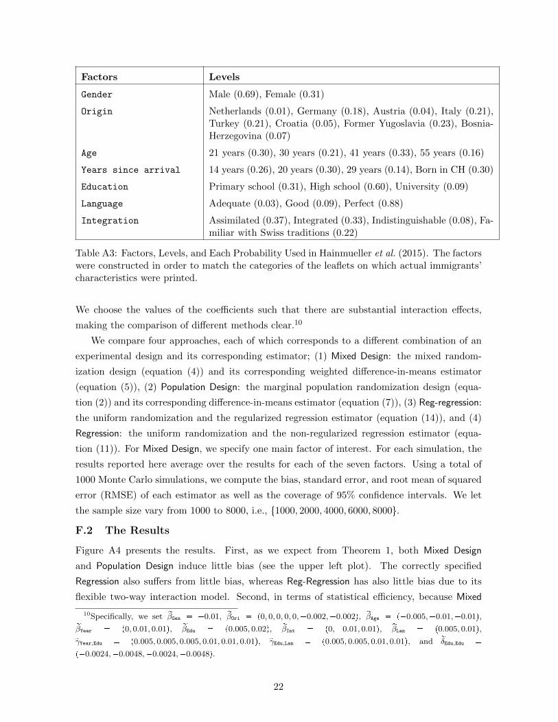
Factors Levels

Gender Male (0.69), Female (0.31)

Origin Netherlands (0.01), Germany (0.18), Austria (0.04), Italy (0.21),Turkey (0.21), Croatia (0.05), Former Yugoslavia (0.23), Bosnia-Herzegovina (0.07)

Age 21 years (0.30), 30 years (0.21), 41 years (0.33), 55 years (0.16)

Years since arrival 14 years (0.26), 20 years (0.30), 29 years (0.14), Born in CH (0.30)

Education Primary school (0.31), High school (0.60), University (0.09)

Language Adequate (0.03), Good (0.09), Perfect (0.88)

Integration Assimilated (0.37), Integrated (0.33), Indistinguishable (0.08), Fa-miliar with Swiss traditions (0.22)

Table A3: Factors, Levels, and Each Probability Used in Hainmueller et al. (2015). The factorswere constructed in order to match the categories of the leaflets on which actual immigrants’characteristics were printed.

We choose the values of the coefficients such that there are substantial interaction effects,

making the comparison of different methods clear.10

We compare four approaches, each of which corresponds to a different combination of an

experimental design and its corresponding estimator; (1) Mixed Design: the mixed random-

ization design (equation (4)) and its corresponding weighted difference-in-means estimator

(equation (5)), (2) Population Design: the marginal population randomization design (equa-

tion (2)) and its corresponding difference-in-means estimator (equation (7)), (3) Reg-regression:

the uniform randomization and the regularized regression estimator (equation (14)), and (4)

Regression: the uniform randomization and the non-regularized regression estimator (equa-

tion (11)). For Mixed Design, we specify one main factor of interest. For each simulation, the

results reported here average over the results for each of the seven factors. Using a total of

1000 Monte Carlo simulations, we compute the bias, standard error, and root mean of squared

error (RMSE) of each estimator as well as the coverage of 95% confidence intervals. We let

the sample size vary from 1000 to 8000, i.e., t1000, 2000, 4000, 6000, 8000u.

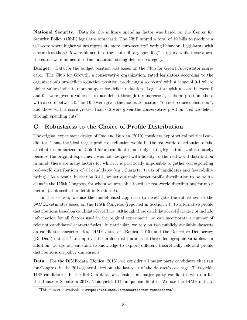
F.2 The Results

Figure A4 presents the results. First, as we expect from Theorem 1, both Mixed Design

and Population Design induce little bias (see the upper left plot). The correctly specified

Regression also suffers from little bias, whereas Reg-Regression has also little bias due to its

flexible two-way interaction model. Second, in terms of statistical efficiency, because Mixed

10Specifically, we set rβGen � �0.01, rβOri � p0, 0, 0, 0, 0,�0.002,�0.002q, rβAge � p�0.005,�0.01,�0.01q,rβYear � p0, 0.01, 0.01q, rβEdu � p0.005, 0.02q, rβInt � p0,�0.01, 0.01q, rβLan � p0.005, 0.01q,rγYear,Edu � p0.005, 0.005, 0.005, 0.01, 0.01, 0.01q, rγEdu,Lan � p0.005, 0.005, 0.01, 0.01q, and rδEdu,Edu �p�0.0024,�0.0048,�0.0024,�0.0048q.

22

●

● ● ● ●

−0.

010

−0.

005

0.00

00.

005

0.01

0

Bias

1000 2000 4000 6000 8000

●

Mixed DesignPopulation DesignReg−regressionRegression

●

●

●

●

●

0.00

0.02

0.04

0.06

0.08

0.10

Standard Error

1000 2000 4000 6000 8000

●

●

●

●

●

0.00

0.02

0.04

0.06

0.08

0.10

RMSE

sample size

1000 2000 4000 6000 8000

●●

●●

●

0.92

0.94

0.96

0.98

1.00

Coverage of 95% Confidence Intervals

sample size

1000 2000 4000 6000 8000

Sample Size Sample Size

Figure A4: Comparison of Four Approaches in terms of Bias, Standard Error, RMSE, andthe Coverage of 95% Confidence Intervals. We evaluate (1) the mixed randomization designand its corresponding weighted difference-in-means estimator (Mixed Design, blue square), (2)the joint population randomization design and its corresponding simple difference-in-meansestimator (Population Design, green diamond), (3) the uniform randomization design and theregularized regression estimator (Reg-regression, red star), and (4) the uniform randomizationdesign and the non-regularized regression estimator (Regression, black circle).

Design focuses on only one factor at a time, it has smaller standard errors than Population

Design (see the upper right plot). Comparing the two model-based estimators, Reg-regression

has smaller standard errors than Regression. The efficiency gain of Reg-regression is achieved

by collapsing indistinguishable levels. In fact, this simulation shows that Reg-regression can

achieve standard errors even smaller than the design-based confirmatory analysis when there

are a lot of redundant levels. However, in some applications like Ono and Burden (2019), the

design-based confirmatory analysis is more efficient. Whenever possible, we recommend the

design-based confirmatory analysis because researchers can always implement the regularized

approach after data collection if necessary. Finally, the coverage of the 95% confidence intervals

is reasonable for all estimators.

23

Supplementary Appendix for - Cambridge University Press

Documents