Supplemental Materials for Local Multidimensional …lc436/papers/LMDS_supplemental.pdf · To explore the effectiveness of LMDS when the underlying structure is known, we rely on

Supplemental Materials for

Local Multidimensional Scaling for

Nonlinear Dimension Reduction, Graph Drawing

and Proximity Analysis

Lisha Chen and Andreas Buja

Yale University and University of Pennsylvania

October 3, 2008

Abstract

In the this supplemental report we include sections that describe (1) a new

interpretation of nonlinear dimension reduction in terms of a population frame-

work as opposed to “manifold learning,” (2) a simulation example based on the

well-known Swissroll to illustrate LMDS on data with known structure, (3) ro-

bustness properties of the LC meta-criterion under an error model. Finally we

include color versions of the plots in the main paper.

1 A Population Framework

Nonlinear dimension reduction can be approached with statistical modeling if

it is thought of as “manifold learning.” Zhang and Zha (2005), for example,

1

examine “tangent space alignment” with a theoretical error analysis whereby

an assumed target manifold is reconstructed from noisy point observations.

With practical experience in mind, we introduce an alternative to manifold

learning and its assumption that the data falls near a “warped sheet.” We

propose instead that the data be modeled by a distribution in high dimensions

that describes the data, warts and all, with variation caused by digitization,

rounding, uneven sampling density, and so on. In this view the goal is to de-

velop methodology that shows what can be shown in low dimensions and to

provide diagnostics that pinpoint problems with the reduction. By avoiding

“prejudices” implied by assumed models, the data are allowed to show what-

ever they have to show, be it manifolds, patchworks of manifolds of different

dimensions, clusters, sculpted shapes with protrusions or holes, general uneven

density patterns, and so on. For an example where this unprejudiced EDA

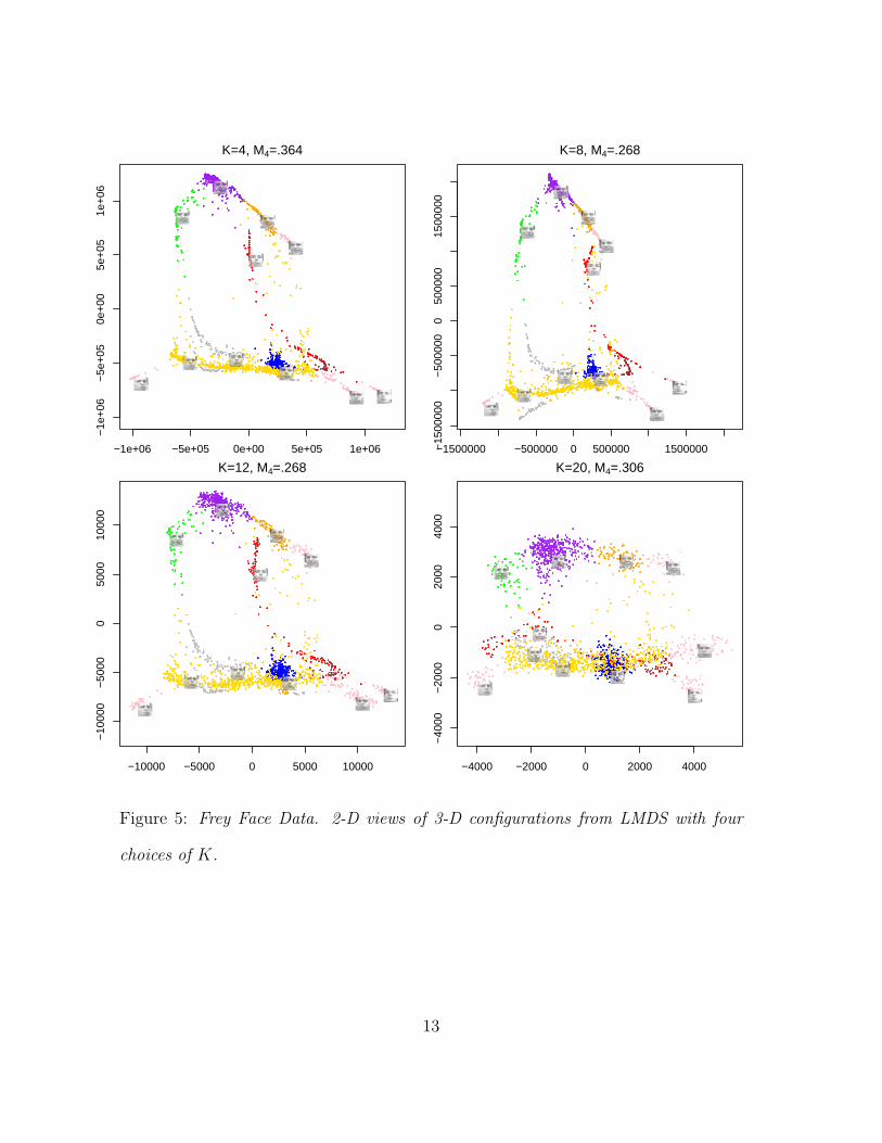
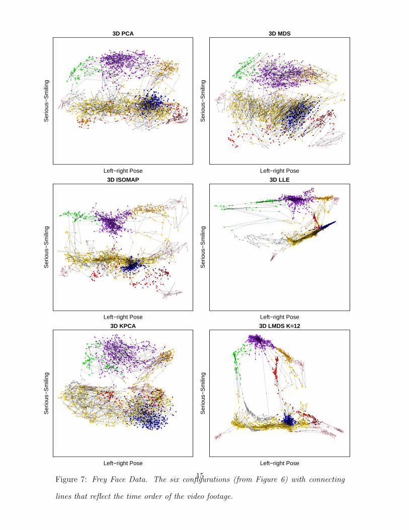
view is successful, see the Frey face image data (Section 4.2, main paper) which

exhibit a noisy patchwork of 0-D, 1-D and 2-D submanifolds in the form of

clusters, rods between clusters, and webfoot-like structures between rods. This

data example also makes it clear that no single dimension reduction may be

sufficient to show all that is of interest: very localized methods (K = 4) reveal

the underlying video sequence and transitions between clusters, whereas global

methods (PCA, MDS) show the extent of the major interpretable clusters and

dimensions more realistically. In summary, it is often pragmatic to assume less

(a distribution) rather than more (a manifold) and to assign the statistician

the task of “flattening” the distribution to lower dimensions as faithfully and

usefully as possible.

An immediate benefit of the distribution view is to recognize Isomap as

non-robust due to its use of geodesic distances. For a distribution, a geodesic

2

distance is a path with shortest length in the support of the distribution. If a

distribution’s support is convex, the notion of geodesic distance in the popula-

tion reduces to chordal distance. For small samples, Isomap may find manifolds

that approximate the high-density areas of the distribution, but for increasing

sample size the geodesic paths will find shortcuts that cross the low-density

areas and asymptotically approximate chordal distances, thus changing the

qualitative message of the dimension reduction as N → ∞.

By comparison, the LMDS criterion has a safer behavior under statistical

sampling as meaningful limits for N → ∞ exist. Here is the population target:

LMDSPN (x) = E

[

(

‖Y ′ − Y ′′‖ − ‖x(Y ′) − x(Y ′′)‖)2

· 1[(Y ′,Y ′′)∈N ]

]

(1)

− t E[

‖x(Y ′) − x(Y ′′)‖ · 1[(Y ′,Y ′′)/∈N ]

]

,

where Y ′, Y ′′ are iid P(dy) on IRp, N is a symmetric neighborhood definition in

IRp, and the “configuration” y 7→ x(y) is interpreted as a map from the support

of P(dy) in IRp to IRd whose quality is being judged by this criterion. When spe-

cialized to empirical measures, LMDSPN (x) becomes LMDSD

N (x(y1), ..., x(yN )).

A full theory would establish when local minima of (1) exist and when those

of (equation 7, main paper) obtained from data converge to those of (1) for

N → ∞. Further theory would describe rates with which N and t can be

shrunk to obtain finer resolution while still achieving consistency.

The LC meta-criteria also have population versions for dimension reduction:

For y in the support of P (dy) (which we assume continuous), let NYα (y) be

the Euclidean neighborhood of y that contains mass α: P [Y ∈NYα (y) ] = α;

similarly, in configuration space let NXα (x(y)) be the mass-α neighborhood of

x(y): P [x(Y )∈NXα (x(y)) ] = α. Then the population version of the LC meta-

3

criterion for parameter α is

Mα =1

αP [Y ′′∈NY

α (Y ′) and x(Y ′′)∈NXα (x(Y ′)) ] ,

where again Y ′, Y ′′ are iid P (dy). This specializes to MK ′ (equation 9, main

paper) for K ′/N = α when P (dy) is an empirical measure (modulo exclusion

of the center points, which is asymptotically irrelevant). The quantity Mα is

a continuity measure, unlike for example the criterion of Hessian Eigenmaps

(Donoho and Grimes 2003) which is a smoothness measure.

A population point of view had proven successful once before in work by

Buja, Logan, Reeds and Shepp (1994) which tackled the problem of MDS per-

formance on completely uniformative or “null” data. It was shown that in the

limit (N → ∞) null data {Di,j} produce non-trivial spherical distributions as

configurations and that this effect is also a likely contributor to the “horseshoe

effect,” the artifactual bending of MDS configurations in the presence of noise.

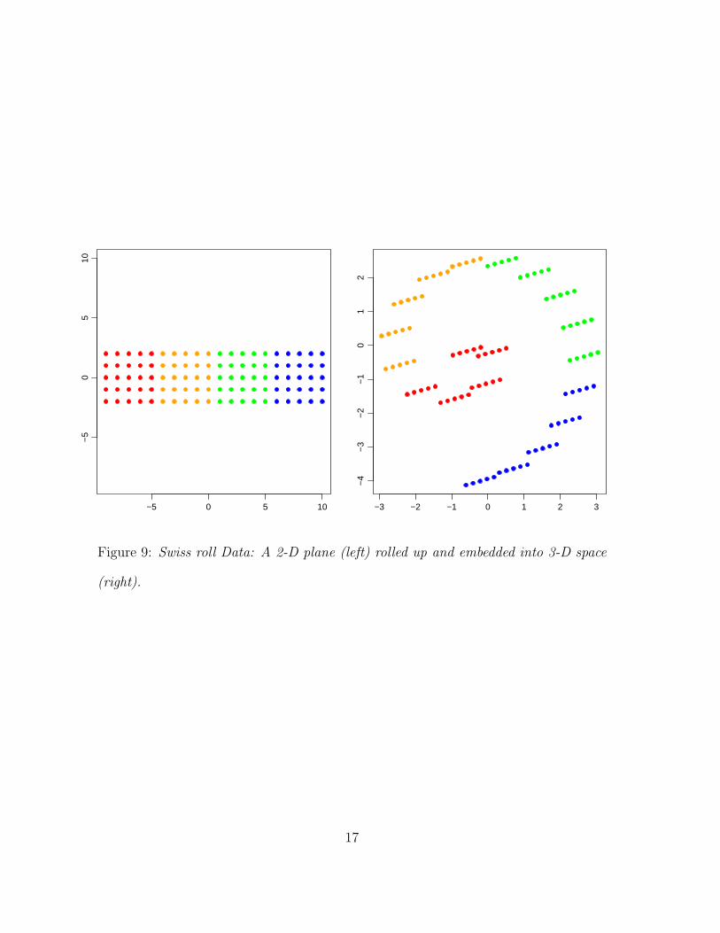
2 A Simulation Example: Swiss Roll Data

To explore the effectiveness of LMDS when the underlying structure is known,

we rely on a simulation example widely used in nonlinear dimension reduction:

the “Swiss roll,” which is a 2-D planar rectangle (Figure 9, left) rolled up and

embedded in 3-D (Figure 9, right). The objective is to recover the intrinsic 2-D

structure from the observed 3-D data. Our data consist of 100 points forming

an equispaced 5 × 20 rectangular grid in parameter space, mapped to 3-D by

warping the long side along a spiral. We color the data points red, orange,

green and blue by dividing the rectangular grid into four chunks of 25 points in

the long dimension. This scheme facilitates visual evaluation of a configuration

generated with a particular method.

4

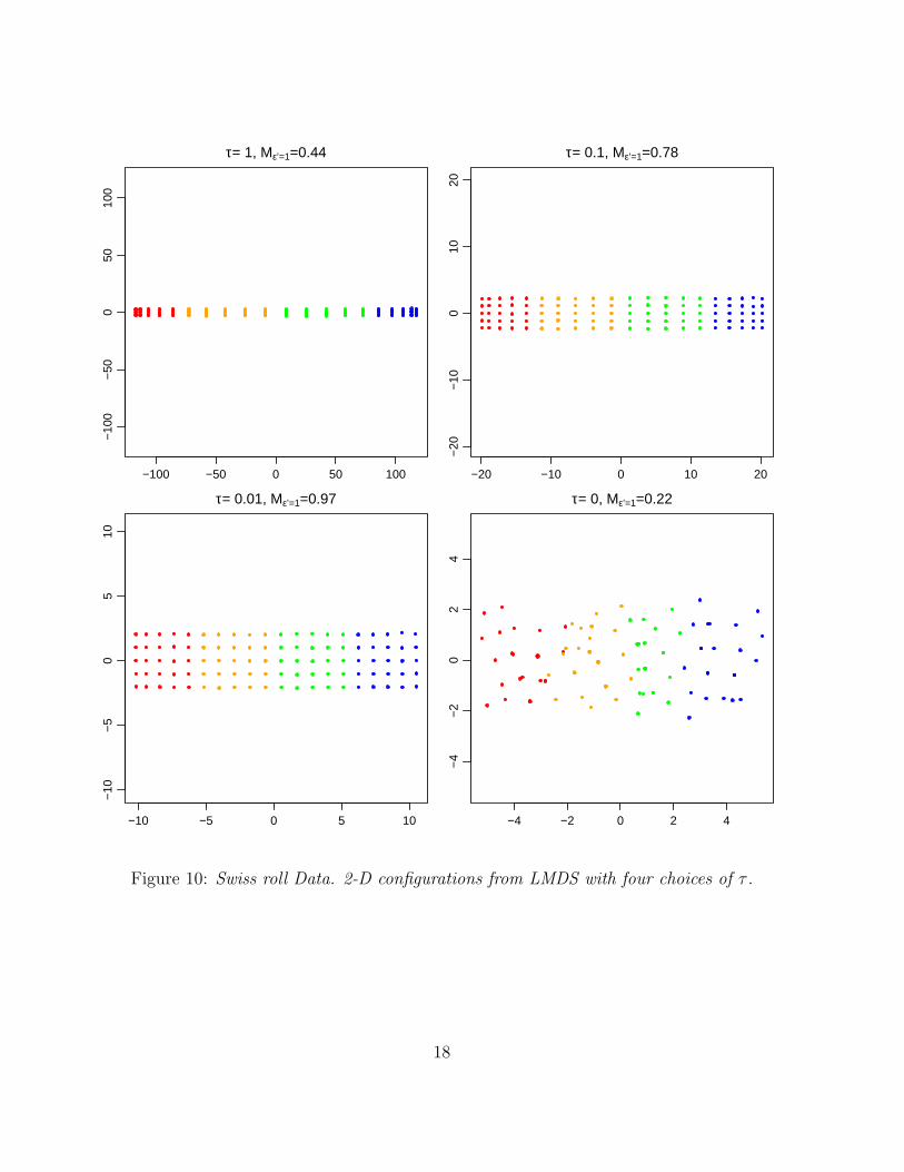
Given the data, we obtain a 2-D configuration by following these steps:

(1) Calculate the Euclidean pairwise distances between the 100 3-D data points.

(2) Define the neighborhood based on metric thresholding (ǫ-NN). More specif-

ically, for any pair of points (i, j), (i, j) ∈ N iff Di,j ≤ ǫ = 1. (We have also

tried K-NN (K = 4) for defining neighborhood, with results slightly inferior

to metric thresholding.) (3) Choose a value for tuning parameter τ . (4) Op-

timize the LMDS stress function to generate a configuration. — In Figure 10

we show the configurations with four different values of τ . We see that the

configurations with relatively larger τ ’s (τ = 1, 0.1) tend to be stretched out

on the long side, which indicates repulsion is too strong. The most desirable

configuration is achieved at τ = 0.01 which is most similar to the intrinsic

2-D structure. With no repulsion (τ = 0) the configurations get trapped in

local minimal, which again indicates that repulsion is essential for achieving

meaningful configurations.

The quality of the configurations as measured by the values of the LC meta-

criterion is consistent with our visual impressions, with larger Mǫ′=1 corre-

sponding to a better configuration. (As in K-NN thresholding, we use ǫ′ for

the calculation of the meta-criterion in distinction of ǫ used in defining the

local graph for the stress function.) This again supports the idea that the LC

meta-criterion provides a good measure for local faithfulness and the quality of

a configuration.

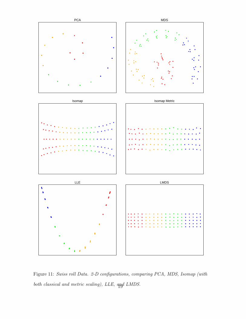
We also compared the configurations generated by LMDS with those of other

dimension reduction methods, including PCA, MDS, Isomap and LLE. The

configurations are shown in Figure 11. PCA provides a linear projection of the

data that captures the greatest variation of the data, which is determined by the

spiral structure. The global structure of the MDS configuration is very similar

5

to the PCA configuration due to the dominance of large distances in the stress

function. For Isomap, we use both the original Isomap method and a slightly

modified version. The latter version uses metric distance scaling instead of

classical scaling to generate the configuration from the shortest path distances.

Interestingly, Isomap with classical scaling produces a double fan shape which

systematically deviates from the underlying true structure. Isomap with metric

distance scaling on the other hand yields a configuration with less distortion,

which is another example of the generally lower desirability of classical scaling

compared to metric scaling. The parabolic shape generated by LLE suggests

that LLE is able to do the unrolling to some extent but not fully, at least not

without further fine tuning (LLE is known to be sensitive to tuning). The

last embedding generated by LMDS is clearly the winner, and it outperforms

its close competitor, the embedding from Isomap metric scaling, in terms of

faithfulness of local structure. While in Isomap metric scaling the local texture

is just a byproduct of the global embedding due to the dominance of the large

geodesic distances in the stress functions, in LMDS one is able to tune τ to

obtain locally faithful configuration. We see this as an appealing feature of

LMDS.

3 Moderate Robustness of the LC Meta-

Criterion

A referee raised the question of robustness of the LC meta-criterion to noise.

In the presence of noise, the set of K nearest neighbors of each data point will

be affected. By measuring the degree of local overlap between neighborhoods

6

of configurations and noise-contaminated data, can the LC meta-criterion still

guide the search for desirable configurations? The referee’s intuition was that

if the noise level exceeds the diameter of the K nearest neighborhoods the

LC meta-criterion will become essentially random. We explored the question

through simulation. The results show that the LC meta-criterion is moderately

robust to noise. It certainly does not become completely random for moderate

noise levels.

In our simulation, we corrupted the true interpoint distances Di,j of the

uncorrupted Swiss roll data with Gaussian noise eD with mean 0 and standard

deviation SD(eD). In order to measure the ability of the LC meta-criterion

to distinguish good from bad configurations, we corrupted the underlying true

2-D configuration (the 5 × 20 regular grid with unit length grid steps) with

Gaussian noise eX with mean 0 and standard deviation SD(eX). The idea is

that the LC meta-criterion is supposed to show a decline for increasing SD(eX),

the steeper the better.

We then calculated the LC meta-criterion MK ′=4 by measuring the overlaps

of K ′ = 4 neighborhoods in terms of the corrupted distances Di,j vis-a-vis the

corrupted grids. Figure 12 shows MK ′=4 as a function of the noise level SD(eX)

in each of the six plots, and as a function of the noise level SD(eD) across the

plots. The noise levels we considered for SD(eX) and SD(eD) range both from

0 to 1, which is commensurate with the fact that the true underlying grid steps

have unit length. Each plot shows the averages and 90% coverage intervals

for Mk′=4 based on 100 simulations. As hoped for, Mk′=4 generally decreases

as SD(eX) increases. When the distances are moderately contaminated with

noise (SD(eD) =0.2, 0.4, 0.6), the LC meta-criterion provides a good measure

of the quality of a configuration, indicated by the overall downward trend of

7

Mk′=4. Only when the noise level is too great (eD = 0.8, 1) does the LC meta-

criterion lose its ability to distinguish good configurations (small SD(eX)) from

bad configurations (large SD(eX)).

It is conceivable that a version of the above simulations could be developed

into a general diagnostics methodology for data analysis. It would provide in-

sight into the robustness of the structure found in terms of a sensitivity analysis.

We thank the referee for suggesting this simulation study which may well lead

to refining the methodology of non-linear dimension reduction in general.

4 Color Plots

We reproduce here the full series of plots of the main paper, but those that

were intended to be in color are rendered here in color. Figures 9 and on are

new and illustrate the Swiss roll experiments in this supplemental report.

REFERENCES

Buja, A., Logan, B.F, Reeds, J.R., Shepp, L.A. 1994, Inequalities and Positive-

Definite Functions Arising from a Problem in Multidimensional Scaling,

The Annals of Statistics, 22, 406-438.

Donoho, D.L., and Grimes, C., 2003, Hessian Eigenmaps: Locally Linear

Embedding Techniques For High-Dimensional Data, Proc. of National

Academy of Sciences, 100 (10), 5591-5596.

Zhang, Z., and Zha, H., 2005, Principal manifolds and nonlinear dimensional-

ity reduction via tangent space alignment. SIAM J. Scientific Computing,

26, 313-338.

8

−50 0 50

−40

−30

−20

−10

0

10

20

30

3D LMDS

Left−right Pose

Up−

dow

n P

ose

−50 0 50

−40

−30

−20

−10

0

10

20

30

Left−right Pose

Ligh

ting

Dire

ctio

n

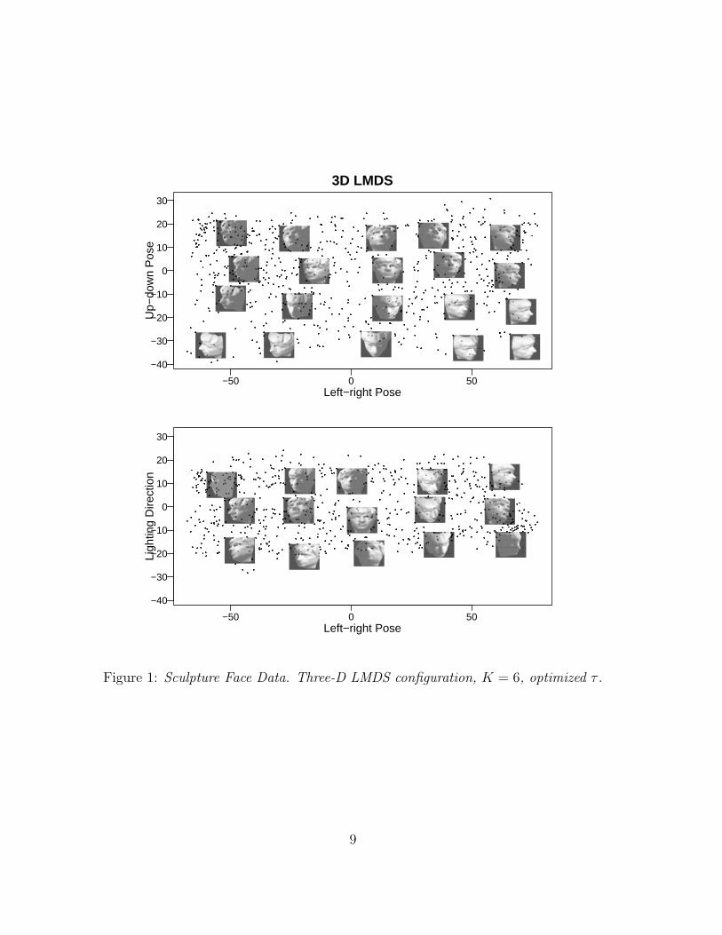
Figure 1: Sculpture Face Data. Three-D LMDS configuration, K = 6, optimized τ .

9

−15

−5

05

10

−15 −5 5 15

−10

05

10

−10 0 5 15

−10

05

10

−10 0 5 15

−2

−1

01

2

−2 −1 0 1 2

−2

−1

01

2

−2 −1 0 1 2

−2

−1

01

2

−2 −1 0 1 2

−50

050

−50 0 50

−30

−10

1030

−30 −10 10 30

−30

−10

1030

−30 −10 10 30

−2

−1

01

2

−2 0 1 2

−1.0

0.01.0

−1.0 0.0 1.0

−1.0

0.01.0

−1.0 0.0 1.0

−0.25

−0.15

−0.05

0.05

−0.25 −0.10 0.00−0.25

−0.15

−0.05

0.05

−0.25 −0.10 0.00−0.25

−0.15

−0.05

0.05

−0.25 −0.10 0.00

Left−right PoseUp−down PoseLighting Direction

PC

AM

DS

LMD

SIS

OM

AP

LLE

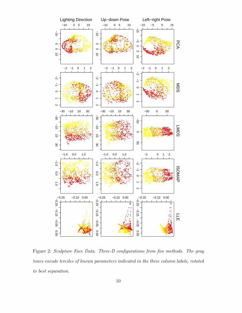
Figure 2: Sculpture Face Data. Three-D configurations from five methods. The gray

tones encode terciles of known parameters indicated in the three column labels, rotated

to best separation.

10

5e−04 5e−03 5e−02 5e−01

0.0

0.2

0.4

0.6

0.8

1.0

K=K’=6

τ

MK

’

5 10 20 50 100 200 500

0.0

0.2

0.4

0.6

0.8

1.0

K’(=K)

MK

’

MK’AdjustedMK’

5 10 20 50 100 200 500

0.0

0.2

0.4

0.6

0.8

1.0

K’

MK

’

K=4K=6K=8K=10K=25K=125K=650

5 10 20 50 100 200 500

0.0

0.2

0.4

0.6

0.8

1.0

K’

Adj

uste

d M

K’

K=4K=6K=8K=10K=25K=125K=650

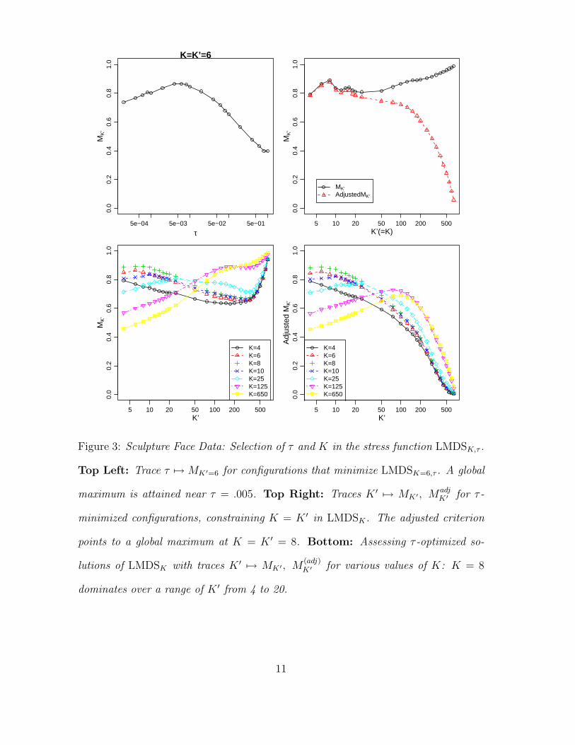
Figure 3: Sculpture Face Data: Selection of τ and K in the stress function LMDSK,τ .

Top Left: Trace τ 7→ MK ′=6 for configurations that minimize LMDSK=6,τ . A global

maximum is attained near τ = .005. Top Right: Traces K ′ 7→ MK ′, MadjK ′ for τ -

minimized configurations, constraining K = K ′ in LMDSK. The adjusted criterion

points to a global maximum at K = K ′ = 8. Bottom: Assessing τ -optimized so-

lutions of LMDSK with traces K ′ 7→ MK ′, M(adj)K ′ for various values of K: K = 8

dominates over a range of K ′ from 4 to 20.

11

−15 −10 −5 0 5 10 15

−15

−10

−5

05

1015

3D PCA (N6=2.6)

−2 −1 0 1 2

−2

−1

01

2

3D ISOMAP (N6=4.5)

−0.05 0.00 0.05

−0.

050.

000.

05

3D LLE (N6=2.8)

−50 0 50

−50

050

3D LMDS (N6=5.2)

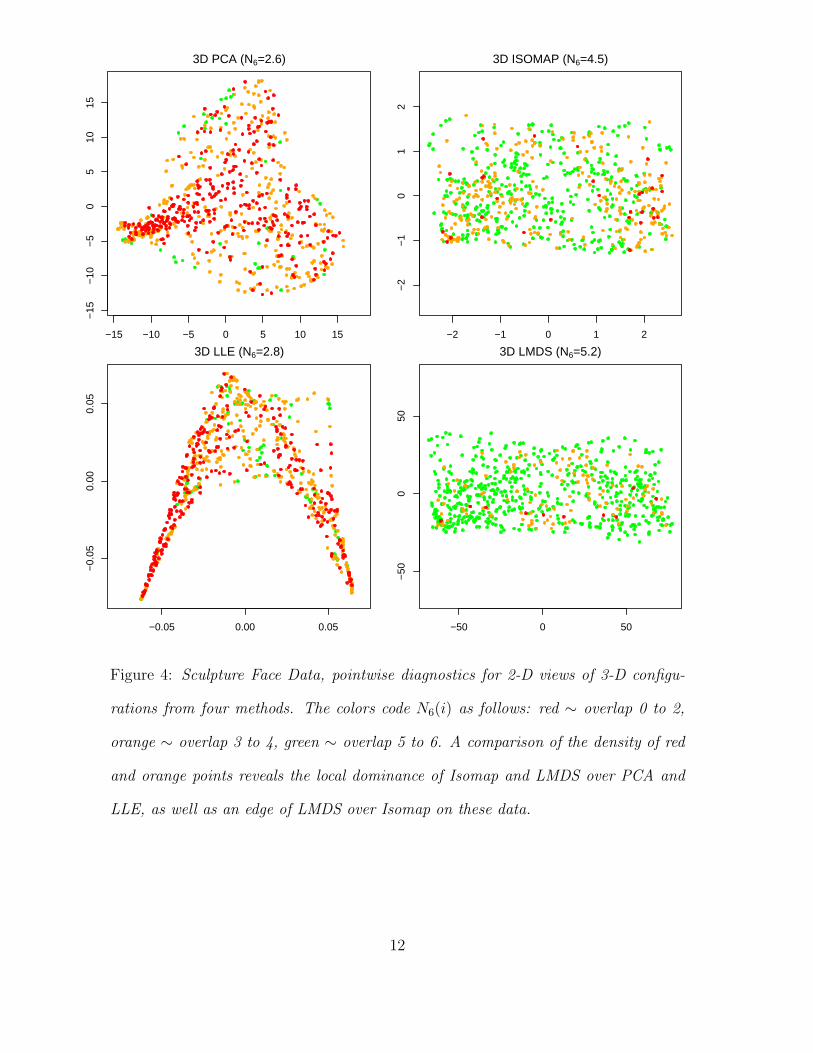
Figure 4: Sculpture Face Data, pointwise diagnostics for 2-D views of 3-D configu-

rations from four methods. The colors code N6(i) as follows: red ∼ overlap 0 to 2,

orange ∼ overlap 3 to 4, green ∼ overlap 5 to 6. A comparison of the density of red

and orange points reveals the local dominance of Isomap and LMDS over PCA and

LLE, as well as an edge of LMDS over Isomap on these data.

12

−1e+06 −5e+05 0e+00 5e+05 1e+06

−1e

+06

−5e

+05

0e+

005e

+05

1e+

06

K=4, M4=.364

−1500000 −500000 0 500000 1500000−15

0000

0−

5000

000

5000

0015

0000

0

K=8, M4=.268

−10000 −5000 0 5000 10000

−10

000

−50

000

5000

1000

0

K=12, M4=.268

−4000 −2000 0 2000 4000

−40

00−

2000

020

0040

00

K=20, M4=.306

Figure 5: Frey Face Data. 2-D views of 3-D configurations from LMDS with four

choices of K.

13

3D PCA

Left−right Pose

Ser

ious

−S

mili

ng

3D MDS

Left−right Pose

Ser

ious

−S

mili

ng

3D ISOMAP K=12

Left−right Pose

Ser

ious

−S

mili

ng

3D LLE K=12

Left−right Pose

Ser

ious

−S

mili

ng

3D KPCA

Left−right Pose

Ser

ious

−S

mili

ng

3D LMDS K=12

Left−right Pose

Ser

ious

−S

mili

ng

Figure 6: Frey Face Data. 2-D views of 3-D configurations, comparing PCA, MDS,

Isomap, LLE, KPCA and LMDS.

14

3D PCA

Left−right Pose

Ser

ious

−S

mili

ng

3D MDS

Left−right Pose

Ser

ious

−S

mili

ng

3D ISOMAP

Left−right Pose

Ser

ious

−S

mili

ng

3D LLE

Left−right Pose

Ser

ious

−S

mili

ng

3D KPCA

Left−right Pose

Ser

ious

−S

mili

ng

3D LMDS K=12

Left−right Pose

Ser

ious

−S

mili

ng

Figure 7: Frey Face Data. The six configurations (from Figure 6) with connecting

lines that reflect the time order of the video footage.

15

5 10 20 50 100

0.3

0.4

0.5

0.6

K’

MK

’

K=4K=8K=12K=20K=50K=100K=150K=1964

5 10 20 50 100

−0.

10−

0.05

0.00

0.05

K’

MK

’ ad

just

ed w

ith M

DS

Figure 8: Frey Face Data. Traces of the Meta-Criterion, K ′ 7→ MK ′, for various

choices of the neighborhood size K in the local stress LMDSK. Left: unadjusted

fractional overlap; right: adjusted with MDS as the baseline. MDS is LMDS with

K=1964, which by definition has the profile MadjK ′ ≡ 0 in the right hand frame.

16

−5 0 5 10

−5

05

10

−3 −2 −1 0 1 2 3

−4

−3

−2

−1

01

2

Figure 9: Swiss roll Data: A 2-D plane (left) rolled up and embedded into 3-D space

(right).

17

−100 −50 0 50 100

−10

0−

500

5010

0

τ= 1, Mε’=1=0.44

−20 −10 0 10 20

−20

−10

010

20

τ= 0.1, Mε’=1=0.78

−10 −5 0 5 10

−10

−5

05

10

τ= 0.01, Mε’=1=0.97

−4 −2 0 2 4

−4

−2

02

4

τ= 0, Mε’=1=0.22

Figure 10: Swiss roll Data. 2-D configurations from LMDS with four choices of τ .

18

PCA MDS

Isomap Isomap Metric

LLE LMDS

Figure 11: Swiss roll Data. 2-D configurations, comparing PCA, MDS, Isomap (with

both classical and metric scaling), LLE, and LMDS.19

0.0 0.2 0.4 0.6 0.8 1.0

0.2

0.4

0.6

0.8

SD(eD)=0

MK

’= 4

0.0 0.2 0.4 0.6 0.8 1.0

0.2

0.4

0.6

0.8

SD(eD)=0.2

0.0 0.2 0.4 0.6 0.8 1.0

0.2

0.4

0.6

0.8

SD(eD)=0.4

MK

’= 4

0.0 0.2 0.4 0.6 0.8 1.0

0.2

0.4

0.6

0.8

SD(eD)=0.6

0.0 0.2 0.4 0.6 0.8 1.0

0.2

0.4

0.6

0.8

SD(eD)=0.8

SD(eX)

MK

’= 4

0.0 0.2 0.4 0.6 0.8 1.0

0.2

0.4

0.6

0.8

SD(eD)=1

SD(eX)

Figure 12: Swiss roll Data. A simulation study on robustness of LC meta-criterion.

eD is the noise added to original 3-D swissroll and eX is the noise added to intrinsic

2-D structure to generate artificial configurations.

20