SUPERSTRUCTURE BRIDGE SELECTION BASED ON BRIDGE LIFE …

SUPERSTRUCTURE BRIDGE SELECTION BASED ON BRIDGE LIFE-CYCLE

COST ANALYSIS

A Dissertation

Submitted to the Faculty

of

Purdue University

by

Stefan Leonardo Leiva Maldonado

In Partial Fulfillment of the

Requirements for the Degree

of

Doctor of Philosophy

August 2019

Purdue University

West Lafayette, Indiana

ii

THE PURDUE UNIVERSITY GRADUATE SCHOOL

STATEMENT OF DISSERTATION APPROVAL

Dr. Mark D. Bowman, Chair

School of Civil Engineering

Dr. Robert J. Frosch


Dr. Robert J. Connor


Dr. Jan Olek


Dr. Wallace E. Tyner

School of Agricultural Economics

Approved by:

Dr. Dulcy M Abraham

Head of the School Graduate Program

iii

To my loved ones, you made this possible.

To Mom who keeps smiling from wherever you are.

To Endrina, the love of my life.

iv

ACKNOWLEDGMENTS

This section is probably one of the most complicated tasks that any person has to

accomplished, not only because is a way to close a huge cycle in your life but because

at the end, it is clearly unfair to express all the gratitude to all who were part of this

incredible, challenging and demanding effort. However, I will try with the best of my

knowledge and the fragility of my memory to remember all of you in these few words.

First, I want to express my most sincere gratitude to my advisor, professor Mark D

Bowman for his truly dedicated tutorship during all these years. Without his encour-

aging guidance, this could not be possible. Also, this could not be possible without

the confidence and encouraging ideas of professor Fabian Consuegra, Purdue alumnus

who makes you understand the high quality of not only this academic program but

also the good heart of the people who has the chance to come to this amazing campus.

My most sincere admiration and gratitude to all my committee members, professors

Wallace Tyner, Jan Olek, Robert Frosch and Robert Connor for being part of this

research and take the time to truly improve this dissertation. All the staff at Purdue

University, especially to Molly Stetler and Jennifer Ricksy for their kindness and help

during all the administrative procedures.

Second, special thanks to Francisco Pena and Daniel Gomez, one of the most

brilliant persons that I ever met and who were a great help during all the coding effort

that otherwise would be a nightmare. Lisa Losada, a person who truly understands

the word friendship, I will miss our delightful and always fun lunch brakes. Rachel

Chicchi, an amazing friend, thanks to her I was able to adapt to this foreign country,

her friendship and inexhaustible patience with this novice English speaker made this

journey a smooth and enjoyable ride. I have no words to describe how grateful I am

with all the friends that I had the pleasure to share time with during all these years,

Camilo, Alejo, David, Diana, Rosario, Lucio, Luis, Andres “the monster”, Sylvia,

v

Clara, Jackeline, Andres D, Marcela F, Juan and many others (this part could be

extended for pages and pages) who make the time in this place a absolute heaven on

earth.

Third, I want to thank all my family members, my father Orlando, my siblings

Edwin and Alexandra and my mother Nubia, you were the reason for all this effort.

Last but not least, all my gratitude and love to Endrina Forti, her company and

love during this journey were the fuel that let me not perish during the hard times,

and the motivation to give the best of me every day.

vi

TABLE OF CONTENTS

Page

LIST OF TABLES . . . . . . . . . . . . . . . . . . . . . . . . . . . . . . . . . . ix

LIST OF FIGURES . . . . . . . . . . . . . . . . . . . . . . . . . . . . . . . . . xi

ABBREVIATIONS . . . . . . . . . . . . . . . . . . . . . . . . . . . . . . . . . . xiv

ABSTRACT . . . . . . . . . . . . . . . . . . . . . . . . . . . . . . . . . . . . xviii

1 INTRODUCTION . . . . . . . . . . . . . . . . . . . . . . . . . . . . . . . . 1

1.1 Objective . . . . . . . . . . . . . . . . . . . . . . . . . . . . . . . . . . 3

1.2 Organization . . . . . . . . . . . . . . . . . . . . . . . . . . . . . . . . 3

2 LITERATURE REVIEW . . . . . . . . . . . . . . . . . . . . . . . . . . . . 5

2.1 Bridge Superstructure Types . . . . . . . . . . . . . . . . . . . . . . . . 5

2.1.1 Steel Bridges . . . . . . . . . . . . . . . . . . . . . . . . . . . . 5

2.1.2 Concrete Bridges . . . . . . . . . . . . . . . . . . . . . . . . . . 10

2.1.3 Deterioration Factors . . . . . . . . . . . . . . . . . . . . . . . . 11

2.1.4 Bridge Life-Cycle Cost Analysis (BLCCA) . . . . . . . . . . . . 16

3 BRIDGE SUPERSTRUCTURE DESIGN ALTERNATIVES . . . . . . . . . 21

3.1 Superstructure Type Selection . . . . . . . . . . . . . . . . . . . . . . . 21

3.1.1 Span Configuration and Span Ranges Selection . . . . . . . . . 22

3.1.2 Bridge Design . . . . . . . . . . . . . . . . . . . . . . . . . . . . 25

4 COST ALLOCATION . . . . . . . . . . . . . . . . . . . . . . . . . . . . . . 29

4.1 Outliers Identification . . . . . . . . . . . . . . . . . . . . . . . . . . . 30

4.2 Design Costs (DC) . . . . . . . . . . . . . . . . . . . . . . . . . . . . . 32

4.3 Construction Costs (CC) . . . . . . . . . . . . . . . . . . . . . . . . . . 33

4.4 Maintenance Costs and Rehabilitation Costs (MC and RC) . . . . . . . 37

4.5 User Costs(UC) . . . . . . . . . . . . . . . . . . . . . . . . . . . . . . . 38

4.6 Probability Distribution Selection . . . . . . . . . . . . . . . . . . . . . 40

vii

Page

4.6.1 Kormogorov-Smirnov (K-S) test for goodness of fit . . . . . . . 41

4.6.2 Anderson-Darling (A-D) test for goodness of fit . . . . . . . . . 42

4.6.3 PDF selection example . . . . . . . . . . . . . . . . . . . . . . . 43

5 DETERIORATION MODELS FOR INDIANA BRIDGES . . . . . . . . . . 48

6 LIFE-CYCLE COST PROFILES FOR INDIANA BRIDGES . . . . . . . . . 54

7 LIFE-CYCLE COST ANALYSIS FOR INDIANA BRIDGES . . . . . . . . . 65

7.1 Interest Rate, Inflation and Discount Rate . . . . . . . . . . . . . . . . 66

7.2 Life-Cycle Cost Analysis Comparison . . . . . . . . . . . . . . . . . . . 67

7.2.1 Equivalent uniform annual return (EUAR) . . . . . . . . . . . . 68

7.2.2 Net present value (NPV) . . . . . . . . . . . . . . . . . . . . . . 68

7.3 Life-cycle cost analysis -Deterministc approach- . . . . . . . . . . . . . 69

7.4 Life-cycle cost analysis -Stochastic analysis . . . . . . . . . . . . . . . . 78

7.4.1 Monte Carlo Simulation (MCS) . . . . . . . . . . . . . . . . . . 78

7.4.2 Stochastic dominance (SD) . . . . . . . . . . . . . . . . . . . . . 80

7.4.3 Superstructure selection . . . . . . . . . . . . . . . . . . . . . . 88

8 SUMMARY AND CONCLUSIONS . . . . . . . . . . . . . . . . . . . . . . 105

8.1 Summary . . . . . . . . . . . . . . . . . . . . . . . . . . . . . . . . . 105

8.2 Conclusions . . . . . . . . . . . . . . . . . . . . . . . . . . . . . . . . 108

8.3 Future Work . . . . . . . . . . . . . . . . . . . . . . . . . . . . . . . . 110

REFERENCES . . . . . . . . . . . . . . . . . . . . . . . . . . . . . . . . . . . 112

A Bridge Design Drawings . . . . . . . . . . . . . . . . . . . . . . . . . . . . 118

B Basic Concepts of Probability . . . . . . . . . . . . . . . . . . . . . . . . . 131

B.1 The Probabilty Density Function (PDF) . . . . . . . . . . . . . . . . 131

B.2 The Cumulative Density Function (CDF) . . . . . . . . . . . . . . . . 132

B.3 The Empirical Cumulative Density Function (ECDF) . . . . . . . . . 132

B.4 Expectation . . . . . . . . . . . . . . . . . . . . . . . . . . . . . . . . 132

B.5 Useful Probability Distributions . . . . . . . . . . . . . . . . . . . . . 133

B.5.1 The Normal distribution . . . . . . . . . . . . . . . . . . . . . 133

viii

Page

B.5.2 The Gamma distribution . . . . . . . . . . . . . . . . . . . . . 134

B.5.3 The Weibull distribution . . . . . . . . . . . . . . . . . . . . . 134

B.5.4 The Lognormal distribution . . . . . . . . . . . . . . . . . . . 135

B.5.5 The Logistic distribution . . . . . . . . . . . . . . . . . . . . . 135

B.5.6 The Inverse Gaussian distribution . . . . . . . . . . . . . . . . 136

B.5.7 The PERT distribution . . . . . . . . . . . . . . . . . . . . . . 136

C Life Cycle Profiles for Indiana Bridges . . . . . . . . . . . . . . . . . . . . 137

D Interest Equations and Equivalences . . . . . . . . . . . . . . . . . . . . . . 148

D.1 Single Payment Compound Amount Factor (SPACF) . . . . . . . . . 148

D.2 Single Payment Present Worth Factor (SPPWF) . . . . . . . . . . . . 148

D.3 Sinking Fund Deposit Factor (SFDF) . . . . . . . . . . . . . . . . . . 149

D.4 Uniform Series Compound Amount Factor (USCAF) . . . . . . . . . 149

D.5 Uniform Series Present Worth Factor (USPWF) . . . . . . . . . . . . 149

D.6 Capital Recovery Factor (CRF) . . . . . . . . . . . . . . . . . . . . . 149

E Example of Life-Cycle Cost Analysis - Deterministic Approach . . . . . . . 151

F Stochastic Dominance Results for Superstructure Selection . . . . . . . . . 177

VITA . . . . . . . . . . . . . . . . . . . . . . . . . . . . . . . . . . . . . . . . 193

ix

LIST OF TABLES

Table Page

2.1 General description of bride elements condition ratings . . . . . . . . . . . 14

3.1 Bridge Design Matrix . . . . . . . . . . . . . . . . . . . . . . . . . . . . . . 26

4.1 Inflation rates . . . . . . . . . . . . . . . . . . . . . . . . . . . . . . . . . . 30

4.2 Summary agency costs - construction costs . . . . . . . . . . . . . . . . . . 33

4.3 Summary agency costs - Prestressed concrete elements costs . . . . . . . . 36

4.4 Summary agency costs - Maintenance and rehabilitation costs . . . . . . . 39

4.5 PDF Selection - Pay item: Concrete type C . . . . . . . . . . . . . . . . . 45

4.6 Probability distribution functions for different pay items. . . . . . . . . . . 46

4.6 continued . . . . . . . . . . . . . . . . . . . . . . . . . . . . . . . . . . . . 47

5.1 Deterioration curves for cast in place concrete deck [17] . . . . . . . . . . . 50

7.1 LCC summary example: simply supported beams -span length 30ft . . . . 70

7.2 Summary of alternatives considered for LCCP selection . . . . . . . . . . . 89

7.3 Stochastic dominance matrix - Continuous beams, span=75-ft . . . . . . . 95

7.4 Results summary - Deterministic and stochastic analysis comparison . . 103

E.1 Initial cost Simply supported beam, span 30 ft. . . . . . . . . . . . . . . 153

F.1 Stochastic dominance matrix - Simply supported beams, span=30-ft . . . 178





F.6 Stochastic dominance matrix - Simply supported beams, span=110-ft . . 183

F.7 Stochastic dominance matrix - Simply supported beams, span=130-ft . . 184

F.8 Stochastic dominance matrix - Continuous beams, span=30-ft . . . . . . 185


x

Table Page




F.13 Stochastic dominance matrix - Continuous beams, span=90-90-ft . . . . 190

F.14 Stochastic dominance matrix - Continuous beams, span=110-ft . . . . . 191

F.15 Stochastic dominance matrix - Continuous beams, span=130-ft . . . . . 192

xi

LIST OF FIGURES

Figure Page

2.1 Folded plate girder. . . . . . . . . . . . . . . . . . . . . . . . . . . . . . . . 6

2.2 Typical bulb tee girder. . . . . . . . . . . . . . . . . . . . . . . . . . . . . 11

2.3 Typical life cycle condition with repairs and renewals. . . . . . . . . . . . . 12

3.1 INDOT database - Bridge structural type summary. . . . . . . . . . . . . . 22

3.2 Span range summary based on NBI database. . . . . . . . . . . . . . . . . 23

3.3 Span distribution summary. . . . . . . . . . . . . . . . . . . . . . . . . . . 24

3.4 Span aspect ratio summary based on INDOT database. . . . . . . . . . . . 25

4.1 Historical cost data Superstructure Concrete Pay Item. . . . . . . . . . . 34

4.2 ECDF (Fn(x)) vs CDF (F (x)), K-S test parameter Dn for Box Beams unitprice . . . . . . . . . . . . . . . . . . . . . . . . . . . . . . . . . . . . . . . 42

4.3 Graphical PDF Selection results - Pay item: Concrete Type C . . . . . . . 44

5.1 Deterioration curves example for steel bridges. . . . . . . . . . . . . . . . . 49

5.2 Deck deterioration example. . . . . . . . . . . . . . . . . . . . . . . . . . . 51

5.3 Deterioration curves example for concrete slab bridges. . . . . . . . . . . . 52

5.4 Deterioration curves example for prestressed concrete beam bridges. . . . . 52

5.5 Deterioration curves example for prestressed concrete box bridges. . . . . . 53

6.1 Life-cycle profile for slab bridges. . . . . . . . . . . . . . . . . . . . . . . . 58

6.2 Life-cycle profile for prestressed concrete I beams with elastomeric bearings. 59

6.3 Life-cycle profile for prestressed concrete box beams. . . . . . . . . . . . . 60

6.4 Lifee-cycle profile for slab bridges. . . . . . . . . . . . . . . . . . . . . . . . 60

6.5 Life-cycle profile for steel structures SDCL. . . . . . . . . . . . . . . . . . . 61

6.6 Life-cycle profile for prestressed concrete I beams including diaphragms. . . 62

6.7 Life-cycle profile for galvanized steel structures. . . . . . . . . . . . . . . . 63

6.8 Life-cycle profile for galvanized steel structures SDCL. . . . . . . . . . . . 63

xii

Figure Page

7.1 Cost-effectiveness for simply supported beams -Span Range 1- Determin-istc Approach. . . . . . . . . . . . . . . . . . . . . . . . . . . . . . . . . . . 72



7.4 Cost-effectiveness for continuous beams -Span Range 1- Deterministc Ap-proach. . . . . . . . . . . . . . . . . . . . . . . . . . . . . . . . . . . . . . . 75



7.7 Latin hypercube sampling for convergence of output mean and standarddeviation of LCCAP SSB slab bridge, 30-ft . . . . . . . . . . . . . . . . . . 80

7.8 Feasible (FS), Efficient (ES) and Inefficient (IS) sets. . . . . . . . . . . . . 81

7.9 FSD example for simply supported beams, span=75-ft. . . . . . . . . . . . 83

7.10 SSD example for simply supported beams, span=45-ft. . . . . . . . . . . . 84

7.11 AFSD example for simply supported beams, span=75-ft. . . . . . . . . . . 86

7.12 ASSD example for simply supported beams, span=90-ft. . . . . . . . . . . 87

7.13 LCCP selection - CDFs concrete groups . . . . . . . . . . . . . . . . . . . 90

7.14 LCCP selection - CDFs structural steel groups . . . . . . . . . . . . . . . . 91

7.15 LCCP selection - Sensitivity analysis structural steel groups . . . . . . . . 92

7.16 LCCP selection - Sensitivity analysis SDCL groups . . . . . . . . . . . . . 93

7.17 LCCP selection - Sensitivity analysis concrete groups . . . . . . . . . . . . 94

7.18 Simulation results, CDFs continuous beams, span=75-ft. . . . . . . . . . . 96

7.19 Superstructure selection chart - Simply supported beams . . . . . . . . . . 99

7.20 Superstructure selection chart - Continuous beams . . . . . . . . . . . . 100

F.1 Simulation results, CDFs simply supported beams, span=30-ft. . . . . . 178



xiii

Figure Page





F.8 Simulation results, CDFs continuous beams, span=30-ft. . . . . . . . . . 185





F.13 Simulation results, CDFs continuous beams, span=90-90-ft. . . . . . . . 190

F.14 Simulation results, CDFs continuous beams, span=110-ft. . . . . . . . . 191

F.15 Simulation results, CDFs continuous beams, span=130-ft. . . . . . . . . 192

xiv

ABBREVIATIONS

AADT Average Annual Daily Traffic

AASHTO American Association of State Highway and Transportation Of-

ficials

AB Prestressed Concrete AASHTO Beams

ABC Accelerated Bridge Construction

ABD Prestressed Concrete AASHTO Beams with Diaphragms

ACI American Concrete Institute

A-D Anderson-Darling Test

ADTT Average Daily Truck Traffic

AFSD Almost First Stochastic Dominance

ASSD Almost Second Stochastic Dominance

ASTM American Society for Testing and Materials

BCR Benefit-Cost Ratio

BD Superstructure Removal Cost

BLCCA Bridge Life-Cycle Cost Analysis

BLS Bureau of Labor Statistics

BR Bearing Replacement Cost

BT Prestressed Concrete Bulb Tee

BTD Prestressed Concrete Bulb Tee with Diaphragms

CB Prestressed Concrete Box Beams

CC Construction Costs

CDF Cumulative Density Function

CLT Central Limit Theorem

CP Full-Depth Concrete Patching Cost

xv

CPI Constumer Price Index

CRF Capital Recovery Factor

DC Design Costs

DR Concrete Deck Reconstruction Cost

DR Discount Rate

ECDF Empirical Cumulative Density Function

ER Cost-Effectiveness Ratio

ES Efficient Set

EUAC Equivalent Uniform Annual Cost

EUAR Equivalent Uniform Annual Return

FP Full Painting Cost

FPG Folded Plate Girder Bridge System

FRC Fiber-Reinforced Concrete

FS Feasible Set

FSD First Stochastic Dominance

IBMS Indiana Bridge Management System

INDOT Indiana Department of Transportation

IQR Interquartile Range

IRR Internal Rate of Return

IS Inefficient Set

K-S Kormogorov-Smirnov Test

LCC Life-Cycle Cost

LCCA Life-Cycle Cost Analysis

LCCAP Life-Cycle Cost Analysis in Perpetuity

LCCP Life-Cycle Cost Profile

LFT Linear Foot

LRFD Load and Resistance Factor Design

MCS Monte Carlo Simulation

ML Most Likely Value

xvi

NBI National Bridge Inventory

NCHRP National Cooperative Highway Research Program

NDOR Nebraska Deparment of Roads

NHS National Highway System

NPV Net Present Value

O Concrete Overlays Cost

PCI Precast Concrete Institute

PDF Probability Density Function

PERT Program Evaluation and Review Technique

PMS Pavement Management Systems

PWC Present Worth of Cost

RC Rehabilitation Costs

SBXG Structural Steel Beam Galvanized

SBXP Structural Steel Beam Painted

SB Slab Bridge

SC Sealing of the Deck Surface Cost

SD Stochastic Dominance

SDCL Simply Supported Span for Dead Load and Continuous for Live

Load Steel Beams

SFDF Sinking Fund Deposit Factor

SFT Square Feet

SL Service Life

SP Spot Painting Cost

SPACF Single Payment Compound Amount Factor

SPGXG Structural Steel Plate Girder Galvanized

SPGXP Structural Steel Plate Girder Painted

SPPWF Single Payment Present Worth Factor

SR Structural Steel Recycle Cost

SSD Second Stochastic Dominance

xvii

SSSBA Short Span Steel Bridge Alliance

SV Salvage Cost

TTC Travel Time Cost

UC User Costs

USCAF Uniform Series Compound Amount Factor

USPWF Uniform Series Present Worth Factor

VOC Vehicle Operation Cost

WC Washing and Cleaning of Deck Surface Cost

xviii

ABSTRACT

Leiva, Stefan Ph.D., Purdue University, August 2019. Superstructure Bridge Selec-tion Based on Bridge Life-Cycle Cost Analysis. Major Professor: Mark D. Bowman.

Life cycle cost analysis (LCCA) has been defined as a method to assess the total

cost of a project. It is a simple tool to use when a single project has different al-

ternatives that fulfill the original requirements. Different alternatives could differ in

initial investment, operational and maintenance costs among other long term costs.

The cost involved in building a bridge depends upon many different factors. More-

over, long-term cost needs to be considered to estimate the true overall cost of the

project and determine its life-cycle cost. Without watchful consideration of the long-

term costs and full life cycle costing, current investment decisions that look attractive

could result in a waste of economic resources in the future. This research is focused

on short and medium span bridges (between 30-ft and 130-ft) which represents 65%

of the NBI INDIANA bridge inventory.

Bridges are categorized in three different groups of span ranges. Different super-

structure types are considered for both concrete and steel options. Types considered

include: bulb tees, AASHTO prestressed beams, slab bridges, prestressed concrete

box beams, steel beams, steel girders, folded plate girders and simply supported steel

beams for dead load and continuous for live load (SDCL). A design plan composed of

simply supported bridges and continuous spans arrangements was carried out. Anal-

ysis for short and medium span bridges in Indiana based on LCCA is presented for

different span ranges and span configurations.

Deterministic and stochastic analysis were done for all the span ranges considered.

Monte Carlo Simulations (MCS) were used and the categorization of the different

superstructure alternatives was done based on stochastic dominance. First, second,

xix

almost first and almost second stochastic dominance rules were used to determined the

efficient set for each span length and all span configurations. Cost-effective life cycle

cost profiles for each superstructure type were proposed. Additionally, the top three

cost-effective alternatives for superstructure types depending on the span length are

presented as well as the optimum superstructure types set for both simply supported

and continuous beams. Results will help designers to consider the most cost-effective

bridge solution for new projects, resulting in cost savings for agencies involved.

1

1. INTRODUCTION

Life cycle cost analysis (LCCA) is a method used to assess the total cost of a project.

LCCA is particularly useful when a single project has different alternatives that fulfill

the original requirements. Different alternatives could vary in initial investment or

cost, operational costs, maintenance costs or other long term costs. This kind of

analysis, when applied to bridge infrastructure projects is called Bridge Life-cycle Cost

Analysis (BLCCA). According to NCHRP Report 483 [1]: Several recent legislative

and regulatory requirements recognized the potential benefits of life-cycle cost analysis

and call for consideration of such analyses for infrastructure investments, including

investments in highway bridge programs. This contemporary tendency has been the

main driving force for the research and use of BLCCA throughout the country. The

current study is focused on efforts to identify the best approach to incorporate BLCCA

in new bridge construction in Indiana.

The true cost of a bridge structure is the cost to build, inspect and maintain the

bridge over the entire lifespan of the bridge. Typically, decisions regarding selection

of the superstructure type when a new or replacement bridge is needed are based

solely upon the initial construction cost, rather than the life-cycle cost. There are

very few data or prior published studies regarding the life-cycle cost of entire bridge

structures in Indiana that utilize different materials. A study to evaluate these costs

would be useful for efficient and cost-effective future planning.

This research is focused on short to medium span bridges (less than 130-ft) which

represents 65% of the NBI Indiana bridge inventory. Bridges are categorized in three

different groups of span ranges. Different superstructure types are considered for both

concrete and steel options. Types considered include: bulb tees, AASHTO prestressed

beams, slab bridges, prestressed concrete box beams, steel beams, steel girders, folded

plate girders and simply supported steel beams for dead load and continuous for live

2

load (SDCL). A design plan composed of simply supported bridges and continuous

spans arrangements was carried out. Analysis for short and medium span bridges in

Indiana based on LCCA is presented for different span ranges and span configurations.

Findings will help designers to consider the most cost-effective bridge solution for new

projects, resulting in cost savings for agencies involved.

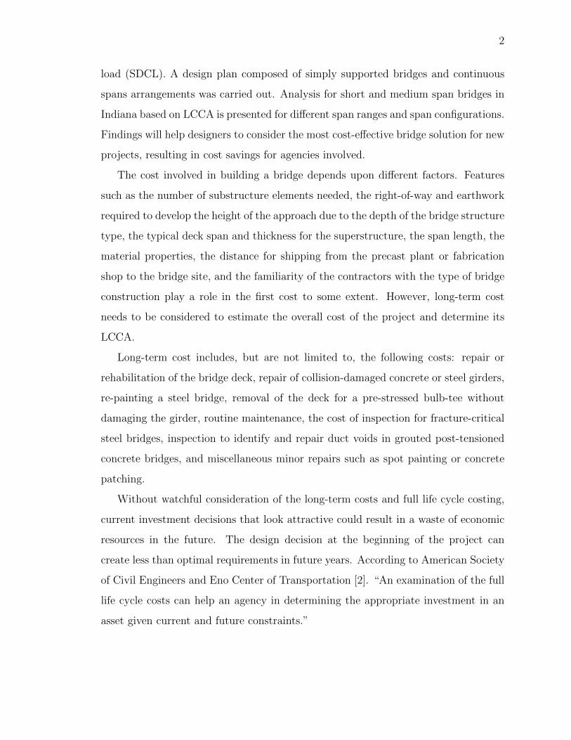
The cost involved in building a bridge depends upon different factors. Features

such as the number of substructure elements needed, the right-of-way and earthwork

required to develop the height of the approach due to the depth of the bridge structure

type, the typical deck span and thickness for the superstructure, the span length, the

material properties, the distance for shipping from the precast plant or fabrication

shop to the bridge site, and the familiarity of the contractors with the type of bridge

construction play a role in the first cost to some extent. However, long-term cost

needs to be considered to estimate the overall cost of the project and determine its

LCCA.

Long-term cost includes, but are not limited to, the following costs: repair or

rehabilitation of the bridge deck, repair of collision-damaged concrete or steel girders,

re-painting a steel bridge, removal of the deck for a pre-stressed bulb-tee without

damaging the girder, routine maintenance, the cost of inspection for fracture-critical

steel bridges, inspection to identify and repair duct voids in grouted post-tensioned

concrete bridges, and miscellaneous minor repairs such as spot painting or concrete

patching.

Without watchful consideration of the long-term costs and full life cycle costing,

current investment decisions that look attractive could result in a waste of economic

resources in the future. The design decision at the beginning of the project can

create less than optimal requirements in future years. According to American Society

of Civil Engineers and Eno Center of Transportation [2]. “An examination of the full

life cycle costs can help an agency in determining the appropriate investment in an

asset given current and future constraints.”

3

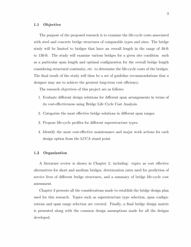
1.1 Objective

The purpose of the proposed research is to examine the life-cycle costs associated

with steel and concrete bridge structures of comparable types and sizes. The bridge

study will be limited to bridges that have an overall length in the range of 30-ft

to 130-ft. The study will examine various bridges for a given site condition such

as a particular span length and optimal configuration for the overall bridge length

considering structural continuity, etc to determine the life-cycle costs of the bridges.

The final result of the study will then be a set of guideline recommendations that a

designer may use to achieve the greatest long-term cost efficiency.

The research objectives of this project are as follows:

1. Evaluate different design solutions for different span arrangements in terms of

its cost-effectiveness using Bridge Life Cycle Cost Analysis.

2. Categorize the most effective bridge solutions in different span ranges.

3. Propose life-cycle profiles for different superstructure types.

4. Identify the most cost-effective maintenance and major work actions for each

design option from the LCCA stand point.

1.2 Organization

A literature review is shown in Chapter 2, including: topics as cost effective

alternatives for short and medium bridges, deterioration rates used for prediction of

service lives of different bridge structures, and a summary of bridge life-cycle cost

assessment.

Chapter 3 presents all the considerations made to establish the bridge design plan

used for this research. Topics such as superstructure type selection, span configu-

rations and span range selection are covered. Finally, a final bridge design matrix

is presented along with the common design assumptions made for all the designs

developed.

4

Cost allocation is summarized in Chapter 4. Description of agency and user costs

are presented. Specifics on values and database usage for every pay item identified

are shown. In addition to common statistic indicators for every pay item, proba-

bility distribution fitting and probability distribution parameterization is done and

presented.

Chapter 5 shows the deterioration models used for different superstructure types,

NBI data and existing deterioration models proposed by different authors are pre-

sented and used.

A literature review on different working actions is presented in Chapter 6. Based

on the deterioration models obtained before, different life-cycle profiles for different

superstructure types are proposed. Finally, the most cost-effective life-cycle profiles

are summarized for different superstructure types.

Chapter 7 presents both deterministic and stochastic approaches used for comput-

ing the life-cycle cost analysis. Deterministic analysis compared not only the life-cycle

cost but also the initial cost for different superstructure types. Additionally, Monte

Carlo simulations are used for the stochastic analysis. Conclusions on both methods

are presented as well as the most cost effective alternatives depending on the bridge

span length.

Finally, Chapter 8 offers a summary of study along with concluding remarks and

suggestions for practitioners.

5

2. LITERATURE REVIEW

This section presents a literature review on innovative cost effective solutions for

short span bridges. Also, a literature review on deterioration curves is included. In

addition, current approaches taken to conduct a Bridge Life Cycle Cost Assessment

are summarized.

2.1 Bridge Superstructure Types

Multiple design solutions have been investigated and used throughout the years

with the objective not only of proposing a structural solution for bridges but also

to provide a cost-effective option for owners and agencies. These two have been the

motivating force of numerous advances in the steel and concrete bridge industries.

Structural systems such as reinforced concrete slab bridges, prestressed concrete bulb

tees, prestressed concrete box beams, prestressed concrete AASHTO beams, steel

beams, steel plate girders and steel box girders have been commonly used across the

country. Nonetheless, the options discussed herein correspond to new technologies

or, in some cases, recent approaches to standard systems that could provide a great

design solution with competitive costs.

2.1.1 Steel Bridges

Folded plate girder (FPG) bridge system

This design approach utilizes U-type shapes built from, cold-bending flat steel

plates into tub sections using a press-brake. According to the Short Span Steel

Bridge Alliance (SSSBA) a maximum span of 60-ft is able to take advantage of this

6

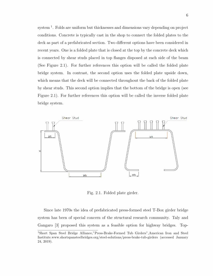
system 1. Folds are uniform but thicknesses and dimensions vary depending on project

conditions. Concrete is typically cast in the shop to connect the folded plates to the

deck as part of a prefabricated section. Two different options have been considered in

recent years. One is a folded plate that is closed at the top by the concrete deck which

is connected by shear studs placed in top flanges disposed at each side of the beam

(See Figure 2.1). For further references this option will be called the folded plate

bridge system. In contrast, the second option uses the folded plate upside down,

which means that the deck will be connected throughout the back of the folded plate

by shear studs. This second option implies that the bottom of the bridge is open (see

Figure 2.1). For further references this option will be called the inverse folded plate

bridge system.

Fig. 2.1. Folded plate girder.

Since late 1970s the idea of prefabricated press-formed steel T-Box girder bridge

system has been of special concern of the structural research community. Taly and

Gangaro [3] proposed this system as a feasible option for highway bridges. Top-

1Short Span Steel Bridge Alliance,”Press-Brake-Formed Tub Girders”,American Iron and SteelInstitute.www.shortspansteelbridges.org/steel-solutions/press-brake-tub-girders (accessed January24, 2019).

7

ics treated includes design basics, fabrication solutions, feasibility study, erection

considerations, bearing types, end joints solutions, curb, parapet and railing types,

maintenance aspects and alternative design procedures.

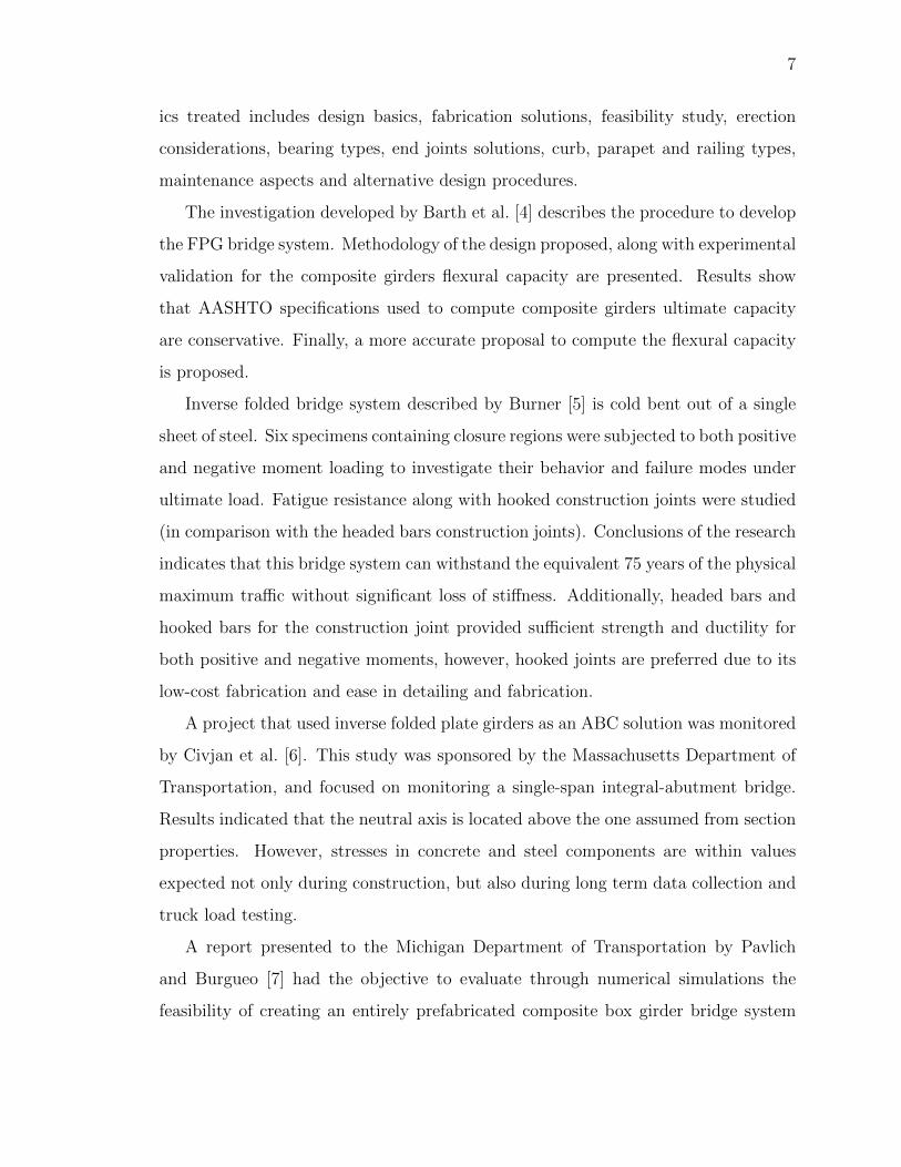
The investigation developed by Barth et al. [4] describes the procedure to develop

the FPG bridge system. Methodology of the design proposed, along with experimental

validation for the composite girders flexural capacity are presented. Results show

that AASHTO specifications used to compute composite girders ultimate capacity

are conservative. Finally, a more accurate proposal to compute the flexural capacity

is proposed.

Inverse folded bridge system described by Burner [5] is cold bent out of a single

sheet of steel. Six specimens containing closure regions were subjected to both positive

and negative moment loading to investigate their behavior and failure modes under

ultimate load. Fatigue resistance along with hooked construction joints were studied

(in comparison with the headed bars construction joints). Conclusions of the research

indicates that this bridge system can withstand the equivalent 75 years of the physical

maximum traffic without significant loss of stiffness. Additionally, headed bars and

hooked bars for the construction joint provided sufficient strength and ductility for

both positive and negative moments, however, hooked joints are preferred due to its

low-cost fabrication and ease in detailing and fabrication.

A project that used inverse folded plate girders as an ABC solution was monitored

by Civjan et al. [6]. This study was sponsored by the Massachusetts Department of

Transportation, and focused on monitoring a single-span integral-abutment bridge.

Results indicated that the neutral axis is located above the one assumed from section

properties. However, stresses in concrete and steel components are within values

expected not only during construction, but also during long term data collection and

truck load testing.

A report presented to the Michigan Department of Transportation by Pavlich

and Burgueo [7] had the objective to evaluate through numerical simulations the

feasibility of creating an entirely prefabricated composite box girder bridge system

8

and employing such system for highway bridges. Topics such as composite girder/deck

joints, vibration characteristics, longitudinal joint of girder/deck units, transversally

posttensioned joints and others were studied. Different longitudinal joint connections

are reviewed including: grouted shear keys, reinforced shear keys, post tensioned

grouted shear keys, welded plate grouted shear key blocks, reinforced grouted moment

key blocks and posttensioned grouted moment keys. Cost, structural performance,

constructability, design ease and other topics were analyzed for spans under 100-

ft. There is not a conclusive selection of joints based on performance or strength.

However, it is concluded that according to the parametric study the performance

of all the different joints considered were adequate for spans ranging from 50-ft to

100-ft..

Other researches like the one published by Nakamura [8] describes a new type of

steel and concrete composite bridge with steel U-shape girders. From the econom-

ical point of view, lack of welding in comparison with regular I-shape girders is an

advantage for this system and therefore very cost-effective. Testing of folded plate

girders replicating loads due to construction without using prefabricated beams were

carried out at the University of Nebraska [9]. Two different plate girder specimens

were tested. To consider proper behavior simulating construction stages, the behav-

ior of the girder alone was evaluated and no concrete slab was cast in any specimen.

The objective of the test was to estimate not only the overall behavior but the girder

components performance. Load levels to cause failure were included, also modes of

failure were reported. Results prove that the folded plate girder provides adequate

strength and stability resistance during construction.

Simply supported span for dead load and continuous for live load (SDCL)

Simple span steel members are utilized at the early construction stages (dead load

only), and then modified by adding the required continuity tension and compression

details during construction to create a continuous structural system. This structural

9

system eliminates field splices when spans are shorter than transportation limitations.

According to the SSSBA normal detailing includes various combinations of anchor

bolts, sole plates and often expensive bearing types. The SDCL method is considered

as a special construction process rather than an application of special bridge elements.

Azizinamini et al. [10] in conjunction with the Nebraska Department of Roads

(NDOR) and the University of Nebraska Lincoln examined a new steel bridge system

which considers simply supported beams for dead load and continuous spans for live

loads. Two full-scale specimens were constructed and tested in order to determine

their structural behavior. Ultimate load tests were conducted to investigate the failure

mechanism. As a result, design equations were developed and verified through finite

element analysis.

Independent design professionals have been proposing SDCL systems as a cost-

effective solution for the bridge industry according to Henkle [11]. For Instance,

Hoorpah et al. (2015) presents the experience with Colville Deverell bridge located in

Mauritius Island. The SDCL system is presented as an economic and fast construction

technology for developing countries. Zanon et al. [12] presented an example of the use

of an SDCL project as part of a new express road construction in Gdansk, Poland.

Some of the points highlighted by this project are mainly focused on the advantage of

prefabrication cost and effective procedures for medium span bridges, especially for

the span range between 80-ft and115-ft.

Finally, a cost-benefit analysis was conducted by Azizinamini et al. [10] for two dif-

ferent structures, a steel box girder superstructure and a steel I-girder superstructure.

It is shown that girders are slightly heavier using the SDCL system in comparison

with the conventional continuous bridge system. However, the elimination of field

splices reduced the total cost of the structural elements by 7% in both cases.

10

2.1.2 Concrete Bridges

A paper summarizing the Japanese state of the art was published by Yamane

et al. [13] on short to medium span (16-ft to 130-ft) precast pre-stressed concrete

bridges. Topics such as construction techniques, design procedures and overall costs

for bridges in Japan and the United States were reviewed. This document presents

a summary of basic geometrical considerations for different bridge types including

typical span ranges.

Bulb tee and hybrid bulb tee beams

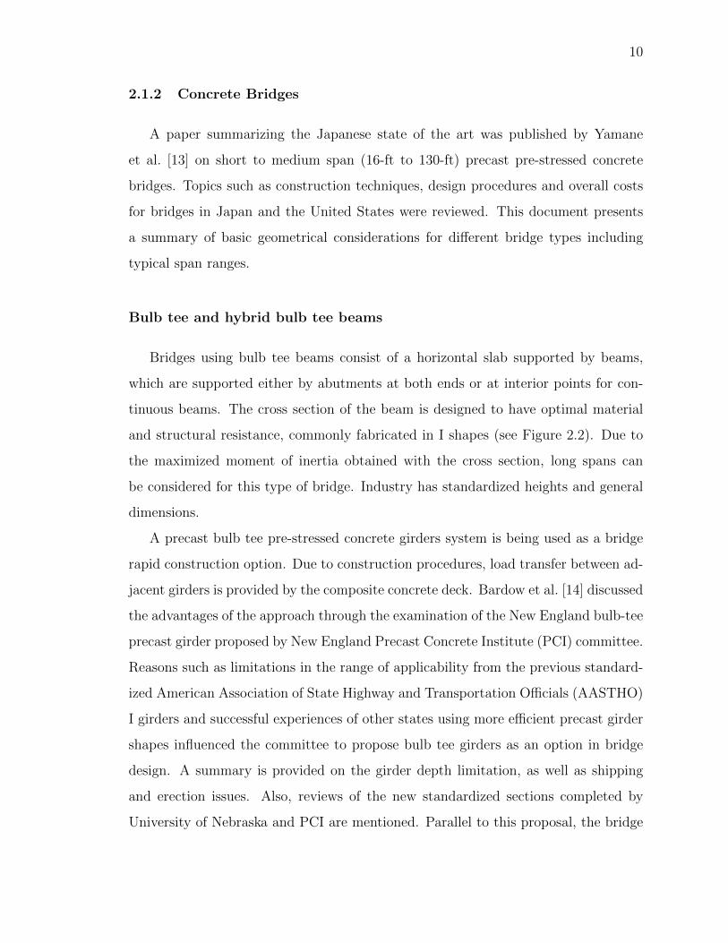
Bridges using bulb tee beams consist of a horizontal slab supported by beams,

which are supported either by abutments at both ends or at interior points for con-

tinuous beams. The cross section of the beam is designed to have optimal material

and structural resistance, commonly fabricated in I shapes (see Figure 2.2). Due to

the maximized moment of inertia obtained with the cross section, long spans can

be considered for this type of bridge. Industry has standardized heights and general

dimensions.

A precast bulb tee pre-stressed concrete girders system is being used as a bridge

rapid construction option. Due to construction procedures, load transfer between ad-

jacent girders is provided by the composite concrete deck. Bardow et al. [14] discussed

the advantages of the approach through the examination of the New England bulb-tee

precast girder proposed by New England Precast Concrete Institute (PCI) committee.

Reasons such as limitations in the range of applicability from the previous standard-

ized American Association of State Highway and Transportation Officials (AASTHO)

I girders and successful experiences of other states using more efficient precast girder

shapes influenced the committee to propose bulb tee girders as an option in bridge

design. A summary is provided on the girder depth limitation, as well as shipping

and erection issues. Also, reviews of the new standardized sections completed by

University of Nebraska and PCI are mentioned. Parallel to this proposal, the bridge

11

Fig. 2.2. Typical bulb tee girder.

portion of the Boston central artery project was designed using the new bulb tees

suggested by the committee. As a result of this cooperation, a standardized bulb tee

sections were adopted, and have been used in numerous projects since then.

2.1.3 Deterioration Factors

Deterioration models for bridges were introduced into the life cycle cost assessment

during the 1980s as a result of the rising interest in predicting the future condition

of infrastructure assets [15]. Nonetheless, those models have been researched prior

to the 80s for pavement management systems (PMS). Difference between these two

approaches focus mainly on the importance of safety, construction materials used and

structural functionality. Even knowing the differences between them, the approaches

used to deal with the deterioration of infrastructure assets (no matter its origin)

are based on the same principles. “By definition, a bridge deterioration model is a

link between a measure of bridge condition that assesses the extent and severity of

damages, and a vector of explanatory variables that represent the factors affecting

12

bridge deterioration such as age, material properties, applied loads, environmental

conditions, etc.” [16].

Deterioration curves have been understood as a model intended to describe the

process and mechanisms by which assets deteriorate and even fail through its service

life. Probabilistic and statistical methods are usually used to accomplish this goal,

leading to a graphical representation of the deterioration of the structure (see example

in Figure 2.3 based on the deterioration curves given by Moomen et al. [17]).

Fig. 2.3. Typical life cycle condition with repairs and renewals.

There are some key components that must be determined to develop a deteriora-

tion model of a structure. The most important of them are the following:

• The anticipated deterioration rate of the element. Known as the pace at which

an asset degrades over time under operating conditions. This must be taken

into account from the beginning of the life of the structure.

13

• The thresholds that define the start and the end of the maintenance stages.

• Actions to take into account at different points and during sequential stages.

The jumps in the deterioration curves are intended to extend the service life of

the asset or to accomplish the overall life cycle objective of the structure.

The basic data used to develop a deterioration prediction is based on the condition

ratings. Condition ratings reflect the deterioration or damage of the structure but not

design deficiencies. To address these scenarios, the National Bridge Inventory (NBI)

classifies them as Structurally Deficient or Functionally Obsolete. Based on field

inspections the condition ratings are considered more like snapshots in time rather

than prediction of future conditions or behavior of the structure.

As a rule, the NBI regulated the condition ratings as a numerical coding from 0

to 9, in which 9 reflects “excellent condition” and 0 represents the “failed condition”

- see Table 2.1. For further details, see the official NBI condition ratings document.

Using condition ratings, it is possible to develop a model that predicts the future

condition of the structure analyzed. The basic representation of this analysis takes

the current condition of the asset and predicts how the condition rating will change

in future years if no maintenance is performed. Some of the options found in the

literature for the predictive modeling include deterministic analysis and stochastic

analysis.

Deterministic analysis

Deterministic analysis models contain no random variables (no probabilities in-

volved) and no degree of randomness. It is dependent on a mathematical formula for

the relationship between the factors affecting the bridge deterioration and the measure

of the condition of the asset. The output obtained is commonly expressed by deter-

ministic values that represent the average predicted condition. This type of model

can be developed using extrapolations, regressions or curve-fitting techniques [15].

14

Table 2.1.General description of bride elements condition ratings

State Description

N Not applicable

9 Excellent Condition

8 Very Good Condition - No problem noted

7 Good Condition - Some minor problems

6 Satisfactory Condition

5 Fair Condition

4 Poor Condition

3 Serious Condition

2 Critical Condition

1 “Imminent” Failure Condition

0 Failed Condition

The Nebraska Department of Transportation sponsored a research project to de-

velop specific models for Nebraskas bridges [18]. This project was focused on the

application of both deterministic and stochastic analysis in bridge decks. Some key

conclusions were made including the significant impact of the traffic volume (AADT

and ADTT) on the deck deterioration. Also, the importance of environmental and

climate changes throughout the state were addressed. It was found that higher traffic

volumes increase the deterioration rate for bridge decks. In addition, in the detailed

report on bridge decks, Morcous [15] also analyzed superstructures and substructures.

Data suggest that prestressed concrete superstructures have similar performance to

steel structures up to condition 6 for Nebraska bridges. Below condition 6 no adequate

condition data for prestressed concrete superstructure were found.

Indiana sponsored a recent project focused on updating bridge deterioration mod-

els though its Department of Transportation [17]. The final report identifies inde-

15

pendent variables such as bridge age, features to cross beneath the bridge, ADTT

among others. This document presents different deterioration curves divided in dif-

ferent groups depending on the material and design types. Curves for decks, different

superstructure types and substructures are summarized. Also, it presents the dif-

ferent significant explanatory variables used for each probabilistic model. Finally,

deterministic and probabilistic case examples are presented using the outcome of the

curves presented. Findings identified trends in the deterioration rates linked to the

independent variables used. Data show that the road classification influences highway

bridge deterioration due to the related ADTT. Higher ADTT values result in higher

deterioration rates. In addition, bridges located over waterways tend to deteriorate

faster than bridges traversing other features.

Stochastic analysis: Markov Chains

A stochastic model traces the projection of variables that can change randomly

with certain probabilities. In this specific case, deterioration progression is set as

one or more stochastic variables that capture the uncertainty of the process. Two

different approximations could be made in this kind of model: state-based and time-

based approximation [19]. State-based models predict the probability that an asset

will undergo a change in condition state at a given time. One of the most known

examples of this model are the Markov chains and the semi-Markov processes. On

the other hand, time-based models predict the probability distribution of the time

taken by an asset to change its condition state. This type of approximation has been

used more frequently in pavement deterioration modeling. However, the two modeling

approaches can be related. It is possible to use one modeling approach to predict the

dependent variable of the other.

A stochastic process can be considered as Markovian if the future behavior depends

only on the present condition but not on the past. In other words, if the state is known

16

at any given time, no more information is needed in order to predict the future state

of the asset [20].

The most important step when a Markov chain method is used is the computation

of the matrix that contains the transition probabilities, which represents the prob-

ability of an element to remain or change from one rating to the other. Transition

probabilities can be obtained either from accumulated condition data or by using an

expert judgment elicitation procedure [15]. Different methods can be used to generate

transition probabilities. However, there are two which have been used to solve this

problem using the condition data available: regression based optimization and per-

centage prediction method. The first one solves the non-linear optimization problem

minimizing the sum of the absolute differences between the regression curve that best

fits the condition data and the predictions using the Markov chains. This method

can be greatly influenced by maintenance that are not reported to the database used.

This means that any change in the data base will have a significant impact in the

outcome. The second approach relates the number of transitions from one state to

another within a given time span with the number of structures in the original state.

Markovians biggest disadvantage is the inherent assumption of the future con-

dition as independent of the historical condition of the asset. The Markov process

assumes, in theory, a programmed and fixed inspection interval for bridges occurs,

but in practice, bridges can be inspected less or more frequently than programmed

for reasons such as financial limitations and technical challenges. The Markov chain

has its merits, such as accounting for the stochastic nature of deterioration, facilita-

tion of the condition characterization of large bridge networks and its computational

efficiency and simplicity [17].

2.1.4 Bridge Life-Cycle Cost Analysis (BLCCA)

For projects related with infrastructure, decision makers often have constrained

budgets. Consequently, decision makers and elected officials often only consider short

17

term cost (a.k.a. initial cost), rather than the long term costs. However, failure to

consider long term costs could lead to decisions that are costlier over the service life

of the structure.

According to the American Society of Civil Engineers and Eno Center of Trans-

portation [2] bridge life cycle cost analysis (BLCCA) is defined as “a data-driven tool

that provides a detailed account of the total cost of a project over its expected life”.

In addition, “BLCCA has been proven to create short-term savings for transportation

agencies and infrastructure owners by helping decision-makers identify the most bene-

ficial and cost effective projects and alternatives.” Numerous transportation agencies

throughout the country have been using BLCCA as a tool for policymakers. BLCCA

has several applications, including:

• Calculating the most cost-effective approaches to project implementation.

• Evaluating a design requirement within a specific project, such as material type

in bridge construction.

• Comparing overall costs between different types of projects to help prioritize

limited funding in an agency-wide program.

Even though BLCCA is presented as a precise tool to allocate budgets, the ap-

proximation itself has different limitations that the agency using it must consider.

The most notorious constraint is the reliability of the prediction of future costs. De-

termination of such predictions are subjected to a substantial estimating risk that

can radically modify the outcome. A second limitation is based on the time horizons

of the analysis. Setting different time horizons can have a dramatic effect on the

analysis results. However, the most important issue is attributed to the lack of trans-

parency and full knowledge of how BLCCA works and how it can be implemented.

It is important to understand that BLCCA must not be considered as an infallible

tool to predict future costs. Nevertheless, it is a helpful instrument to provide better

information to decision-makers.

18

BLCCA is based upon a series of factors that need to be quantified and investi-

gated. First, there is a need to identify alternatives, not only of the structural type

or material but also bridge maintenance and improvement that may vary with the lo-

cations depending on weather conditions and contractors experience. Second, agency

costs need to be addressed. These are (but not limited to) maintenance, rehabilita-

tion and replacement costs. “Most routine maintenance activities are performed by

an agencys own workforce. Rehabilitation works consist of minor and major repair

activities that may require the assistance of design engineers and contractors for con-

struction. Most rehabilitation work is deck related. A major rehabilitation activity

may involve deck replacement. The term bridge replacement” is, on the other hand,

reserved for a complete replacement of the entire bridge structure [1].

An accurate estimation and prediction of such prices is a difficult task since they

tend to fluctuate. Moreover, those prices are connected with the length and type of

bridge work programed in each of the alternatives. Finally, user costs that are the

value of time lost by the user due to delays, detours and road work. There are other

costs such as salvage costs, staffing, tax implications, downtime and so forth, that

would be present in the BLCCA depending on the government dispositions.

General models for BLCCA are summarized as the sum of nonrecurring cost and

recurring costs. The final cost is the result of adding the construction costs, mainte-

nance costs and rehabilitation costs among others. Those cost must include not only

appropriate agency costs but also user costs. Specifically, the model for bridges is

presented in Equation 2.1 [1].

LCC = DC + CC +MC +RC + UC + SV (2.1)

were:

LCC: Life-Cycle Cost

DC: Design Cost

CC: Construction Cost

19

MC: Maintenance Cost

RC: Rehabilitation Cost

UC: User Cost

SV : Salvage Cost

Measurements commonly used for alternative selection are: net present value

(NPV), equivalent uniform annual cost (EUAC) and incremental rate of return.

Life-cycle cost profiles (LCCP)

Life-cycle profiles were conceived as graphical representation of all the costs in-

volved during the service life of a given structure. Those include not only the major

correcting actions (e.g. reconstruction of an element, construction of overlays, bridge

replacement) but also routine working actions characteristic of the bridge life. The

combination of different maintenance, preventive or major corrective actions creates

a unique profile that can be considered. Accurate estimation of service lives for all

the working actions is a combination of agency experience, research efforts and engi-

neering judgment.

Bridges typically involve three different elements that could have different working

actions to consider: deck, superstructure, and substructure. It is true that a combina-

tion of all of them results in a complete LCCA. However, this research is only focused

on the deck and the superstructure. Superstructure working actions often involve the

full or partial intervention of the deck. Therefore, life-cycle profiles proposed here on

are a combination of preventive / maintenance / repair / rehabilitation strategies of

both elements.

The following are the crucial factors to consider when a life cycle profile is pro-

posed: the service life of the structure, working actions considered, life-cycle of the

treatments proposed, proposed schedule of major working actions and possible exten-

sions of the structure service life due to preventive or corrective procedures.

20

The service life of the structures considered corresponds to the age at which the

deterioration curve used reaches the limiting condition rating. According to Indiana

experience, the limiting condition rating that triggers the scheduling of a working

actions corresponds to Poor Condition (condition rating 4). It is true that this condi-

tion does not mean imminent failure or a collapse but it is considered a safe threshold

to assure safety standards.

21

3. BRIDGE SUPERSTRUCTURE DESIGN

ALTERNATIVES

3.1 Superstructure Type Selection

Information obtained from the National Bridge Inventory (NBI) was used to sum-

marize the most common structures within the state and generate a bridge design

matrix for the structures to analyze. The NBI database is an open source information

that can be found in the National Bridge Inventory webpage and can be used freely.

The Indiana Department of Transportation (INDOT) has been collecting infor-

mation on highway construction projects since 2011. This information has been or-

ganized and compiled in a single database that includes not only the total cost of

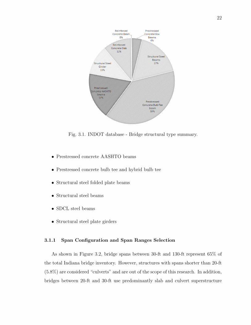
different projects but also discretizes pay items involved. As can be seen in Figure

3.1, the INDOT database shows a predominant use of concrete that represents 72%

of the bridge contracts built from 2011 to 2015. In contrast, structural steel was used

only 28% of the time. This tendency can be seen at a network level also analyzing

the NBI database. According to NBI data, approximately 67% of the structures are

concrete or prestressed concrete bridges (distributed almost evenly) while 30% are

structural steel. This trend may be driven by the first cost effectiveness of concrete

in comparison with structural steel.

The designs selected for this study represent the most common structures found in

Indiana (as shown in Figure 3.1), as well as other bridge design options. It should be

noted, however, that design options for timber, masonry, aluminum or other materials

are not considered. Bridge types used are the following:

• Slab bridge

• Prestressed concrete box beams

22

Fig. 3.1. INDOT database - Bridge structural type summary.

• Prestressed concrete AASHTO beams

• Prestressed concrete bulb tee and hybrid bulb tee

• Structural steel folded plate beams

• Structural steel beams

• SDCL steel beams

• Structural steel plate girders

3.1.1 Span Configuration and Span Ranges Selection

As shown in Figure 3.2, bridge spans between 30-ft and 130-ft represent 65% of

the total Indiana bridge inventory. However, structures with spans shorter than 20-ft

(5.8%) are considered “culverts” and are out of the scope of this research. In addition,

bridges between 20-ft and 30-ft use predominantly slab and culvert superstructure

23

types (82% of the time). Consequently, bridges between 30-ft and 130-ft were selected

as the objective of this study.

To categorize different design options, three different span ranges were established

each with different ranges of maximum span lengths. Range 1 included bridges with

spans within 30-ft and 60-ft, range 2 with span lengths between 60-ft and 90-ft, and

range 3 spans with lengths in the range from 90-ft to 130-ft. Design types were

selected depending on their cost-effectiveness potential for each of the span ranges.

Fig. 3.2. Span range summary based on NBI database.

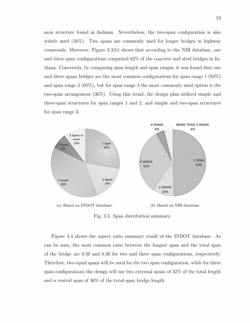
Figure 3.3(a) shows the bridge span distribution within the state for bridges con-

structed in the last 6 years. It is clear that bridges with 4 or more spans are less

common. Simple span (28%) and three-span arrangements (38%) are the most com-

24

mon structure found in Indiana. Nevertheless, the two-span configuration is also

widely used (16%). Two spans are commonly used for longer bridges in highway

crossroads. Moreover, Figure 3.3(b) shows that according to the NBI database, one

and three span configurations comprised 82% of the concrete and steel bridges in In-

diana. Conversely, by comparing span length and span ranges, it was found that one

and three spans bridges are the most common configurations for span range 1 (94%)

and span range 2 (65%), but for span range 3 the most commonly used option is the

two-span arrangement (36%). Using this trend, the design plan utilized simple and

three-span structures for span ranges 1 and 2, and simple and two-span structures

for span range 3.

(a) Based on INDOT database. (b) Based on NBI database.

Fig. 3.3. Span distribution summary.

Figure 3.4 shows the aspect ratio summary result of the INDOT database. As

can be seen, the most common ratio between the longest span and the total span

of the bridge are 0.50 and 0.30 for two and three span configurations, respectively.

Therefore, two equal spans will be used for the two span configuration, while for three

span configurations the design will use two external spans of 32% of the total length

and a central span of 36% of the total span bridge length.

25

Fig. 3.4. Span aspect ratio summary based on INDOT database.

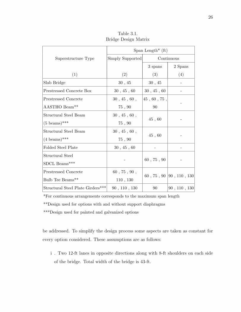
The final design plan includes bridge designs developed for extreme span ranges

values and a single intermediate point along the range. Table 3 presents a summary

of the designs developed for the simply supported configuration. As shown, different

superstructure types are considered depending on its potential cost effectiveness for

each span length. The same approach was used for the continuous span configuration

design plan shown in Table 3.1. The span length shown in Table 3.1 corresponds to

the maximum span length within the multiple spans and not the total length of the

bridge.

3.1.2 Bridge Design

Bridge designs were then developed for the design plan. The seventh edition

AASHTO LRFD specifications [21] and the Indiana Design Manual [22] were used

for the designs. There are some simplifications and assumptions made that need to

26

Table 3.1.Bridge Design Matrix

Span Length* (ft)

Superstructure Type Simply Supported Continuous

3 spans 2 Spans

(1) (2) (3) (4)

Slab Bridge 30 , 45 30 , 45 -

Prestressed Concrete Box 30 , 45 , 60 30 , 45 , 60 -

Prestressed Concrete 30 , 45 , 60 , 45 , 60 , 75 ,-

AASTHO Beam** 75 , 90 90

Structural Steel Beam 30 , 45 , 60 ,45 , 60 -

(5 beams)*** 75 , 90

Structural Steel Beam 30 , 45 , 60 ,45 , 60 -

(4 beams)*** 75 , 90

Folded Steel Plate 30 , 45 , 60 - -

Structural Steel- 60 , 75 , 90 -

SDCL Beams***

Prestressed Concrete 60 , 75 , 90 ,60 , 75 , 90 90 , 110 , 130

Bulb Tee Beams** 110 , 130

Structural Steel Plate Girders*** 90 , 110 , 130 90 90 , 110 , 130

*For continuous arrangements corresponds to the maximum span length

**Design used for options with and without support diaphragms

***Design used for painted and galvanized options

be addressed. To simplify the design process some aspects are taken as constant for

every option considered. These assumptions are as follows:

i . Two 12-ft lanes in opposite directions along with 8-ft shoulders on each side

of the bridge. Total width of the bridge is 43-ft.

27

ii . Concrete bridge railing type FC was used per Indiana Design Manual and

Standard Drawing No. E 706-BRSF-01.

iii . Skew: 0. INDOT database shows that most of the Indiana bridges have skew

values less than 30 which in practical design terms will not significantly impact

the final design.

iv . Moderate ADTT.

v . Concrete deck of 8-in, minimum longitudinal reinforcement of 5/8 and max-

imum rebar spacing of 8-in as the minimum required per the Indiana Design

Manual.

vi . Structural steel ASTM A709 Grade 50. Modulus of Elasticity: 29,000ksi, Fy:

50ksi and Fu: 65ksi.

vii . Reinforcement steel AASHTO A615 Grade 60. Modulus of Elasticity: 29,000

ksi, Fy: 60ksi and Fu: 80ksi.

viii . Prestressing Strands: Low relaxation strands. Modulus of Elasticity: 28,500

ksi, Fy: 243ksi and Fu: 270ksi.

ix . Slab concrete fc: 4ksi, Modulus of Elasticity: 3,834ksi.

x . Concrete prestressed beams fc: 7ksi. Modulus of Elasticity: 5,072ksi. Condi-

tions at transfer may vary.

The research described herein is focused on the superstructure only; the substruc-

ture was not designed for any of the bridges considered. Generalization of soil and

foundation types throughout Indiana is not within the scope of this research.

Spread sheets that include applicable sections of the LRFD and the Indiana Design

Manual specifications were created for every design option. As an input, live load

envelopes were generated using a simple beam element model in SAP2000 R©. The

models were also used to check deflection limits. Limit states checked are: service

28

level, strength level, and fatigue and fracture. Different design examples were con-

sidered as a basis for the designs. Examples include those from Wassef [23], Florida

Department of Transportation [24], Hartle et al. [25], Parsons Brikinckerhoff [26],

Chavel and Carnahan [27], Grubb and Schmidt [28] and Wisconsin Departement of

Transportation [29] were used.

As noted above, detailed bridge designs were developed for each of the options

considered in the design plan. This involved the design of 64 bridges in total. Sum-

mary information from the designs can be found in the design drawings in Appendix

A. Due to the length of each design, the detailed spread sheet designs for each bridge

are available by request and not annexed to this document.

29

4. COST ALLOCATION

As noted earlier, the cost allocation model used herein is described in equation 2.1.

Then, the final life-cycle cost for each alternative would be the sum of the agency

costs, which includes design costs (DC), construction costs (CC), maintenance costs

(MC), rehabilitation costs (RC) salvage costs (SC), and user costs (UC). Unless there

is a reason to do otherwise, agency costs are typically assumed to be incurred at the

end of the period in which expenditures actually will occur [1].

The most widely used basis to estimate those costs are the utilization of unit costs

and bills of quantities. In the absence of this information, parametric cost estimating

models may be used as a best-guess estimate [1]. This study is focused on the highway

bridge system costs in Indiana. The Indiana Department of Transportation (INDOT)

has been collecting information on highway construction projects since 2011. This

information has been organized and compiled in a single database that includes not

only the total cost of different projects but also discretizes pay items involved. Using

this information, it is possible to identify the cost trend of basic pay items such as

concrete, structural steel, structural elements among others.

In order to obtain the current price for each one of the values from the database,

inflation rates need to be used. Inflation rates were calculated using the current

consumer price index (CPI) published monthly by the Bureau of Labor Statistics

(BLS). Values presented in Table 4.1 correspond to the average value throughout the

year. Table 4.1 also presents the cumulative multiplier factor used to compute the

net present value.

30

Table 4.1.Inflation rates

YEAR INFLATION RATE

OF OCCURRENCE Yearly Rate (%) NPV Factor

2017 2.10 1.0210

2016 1.30 1.0343

2015 0.12 1.0355

2014 1.62 1.0523

2013 1.47 1.0678

2012 2.07 1.0899

2011 3.16 1.1243

2010 1.60 1.1423

2009 -0.40 1.1377

2008 3.80 1.1810

2007 2.80 1.2140

2006 3.20 1.2529

2005 3.40 1.2955

2004 2.70 1.3304

2003 2.30 1.3610

2002 1.60 1.3828

2001 2.80 1.4215

2000 3.40 1.4699

1999 2.20 1.5022

4.1 Outliers Identification

The definition of an outlier is at best a subjective idea. However, different inves-

tigators have been addressing this problem from different perspectives. One of the

most accepted definitions of this term is presented by D’Agostino and Stephens [30]:

“a discordant observation is one that appears surprising or discrepant to the investi-

31

gator; a contaminant is one that does not come from the target population; an outlier

is either a contaminant or a discordant observation.” Once the outliers are identified

there are different paths to treat the database shown as follows:

i . Omit the outliers and treat the reduced sample as a new database

ii . Omit the outliers and treat the reduced sample as a censored sample

iii . Replace the outliers with the value of the nearest good observation (Also

called Winsorize the outliers)

iv . Take new observations to replace the outliers and,

v . Do two different analyses with and without outliers. If results are clearly

different the conclusions need to be examined cautiously

Due to the source of the database used in this research the outliers will be identified

and the reduced sample treated as a new database. There are multiple techniques

to identify outliers in a sample which includes: Pierces criterion, modified Thompson

Tau test, anomaly detention among others. Nevertheless, the method used for this

sample was the implementation of the interquartile range (IQR) and the Tukeys fence

approximation. The IQR is the difference between the first and the third quartile.

The first Q1 and third quartile Q3 are the values in the database that holds 25%

and 75% of the values below it respectively. According to the Tukeys fences method,

outliers are values outside of the limits represented by 1.5 times the IQR below Q1

and above Q3. The generalization of the method is presented in Equations 4.1 to 4.3.

IQR = Q3 −Q1 (4.1)

LimBot = Q1 − 1.5(IQR) (4.2)

LimTop = Q3 + 1.5(IQR) (4.3)

Once the database is cleaned from outliers, a standard deviation and mean is

computed for all the pay items involved. However, and in order to take into account

32

the economics of size of the projects, a weighted average and standard deviation

are chosen to use as an input in the BLCCA. The usage of a weighted average is

based on the fact that larger projects would have a more significant impact on the

computation of the mean than smaller projects, which could result in costlier unit

prices. Weights are calculated based on the quantities for each one of the activities

considered. Basic definition of weighted average (µw) and standard deviation (σw) is

presented in Equations 4.4 and 4.5 where xi represents a single value in the database

and wi is the weight associated to that specific value. Weights, as mentioned before,

correspond to the ratio between the individual quantity of the data point and the

total sum of quantities.

µw =

∑ni=1wixi∑ni=1wi

(4.4)

σw =

√∑ni=1wi(xi − µw)2∑n

i=1wi(4.5)

4.2 Design Costs (DC)

Includes all the engineering and regulatory studies, environmental and other re-

views, and consultant contracts prior to the construction or major rehabilitation of

an asset. It is a common practice to compute these values as a percentage of the con-

struction cost when no data are available. However, these costs are not considered in

the computation of the total LCCA for two reasons: Firstly, designs are made by the

researchers and no cost is involved or considered due to such activities, however, in

real projects this cost must be included. Secondly, since this research is not localizing

the design structure in any specific location, environmental and other reviews along

with consultant contracts are not needed.

33

4.3 Construction Costs (CC)

Includes all the activities made between the design and the operation of the asset.

In a project, it may include bridge elements, ancillary facilities, and approach roads

among others. In this study only major superstructure elements are considered.

Substructure construction is neglected since this design is outside of the scope of

the project. Barriers and other miscellaneous items are neglected also due to that

all the alternatives share the same specifications, in other words, they will have the

same elements in the same quantities. Pay items considered include: slab concrete,

structural concrete elements, reinforcing steel and structural steel. Table 4.2 shows

the summary of the construction cost for different superstructure elements. All pay

items shown include all the activities needed until the elements are cast or erection

of the element on site. No additional costs need to be considered due to erection of

superstructure beams or provisional formwork for cast in place elements, since these

costs are included in the pay item price.

Table 4.2.Summary agency costs - construction costs

ITEM UNITUNIT PRICE ($/Unit)

DataMin. Max. µ µm σm

Concrete Type C superstructure yd3 354.25 898.76 589.04 564.03 109.61 354

Prestressed concrete bulb-T beam LFT 188.86 419.06 294.98 298.99 54.86 132

Prestressed concrete box beam SFT 139.03 320.99 241.37 241.51 54.86 13

Prestressed concrete AASHTO beam LFT 107.53 346.43 221.07 219.21 66.93 55

Structural steel lbs 0.64 3.00 1.94 1.72 0.44 63

Reinforcing steel lbs 0.65 1.34 0.96 0.92 0.12 150

Epoxy reinforcing steel lbs 0.74 1.40 1.05 1.02 0.13 324

A further analysis was done for the pay item related to the concrete of the su-

perstructure. As a common practice it is assumed that concrete cost depends on the

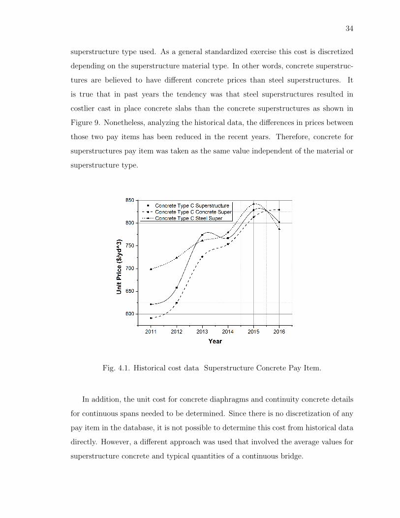
34

superstructure type used. As a general standardized exercise this cost is discretized

depending on the superstructure material type. In other words, concrete superstruc-

tures are believed to have different concrete prices than steel superstructures. It

is true that in past years the tendency was that steel superstructures resulted in

costlier cast in place concrete slabs than the concrete superstructures as shown in

Figure 9. Nonetheless, analyzing the historical data, the differences in prices between

those two pay items has been reduced in the recent years. Therefore, concrete for

superstructures pay item was taken as the same value independent of the material or

superstructure type.

Fig. 4.1. Historical cost data Superstructure Concrete Pay Item.

In addition, the unit cost for concrete diaphragms and continuity concrete details

for continuous spans needed to be determined. Since there is no discretization of any

pay item in the database, it is not possible to determine this cost from historical data

directly. However, a different approach was used that involved the average values for

superstructure concrete and typical quantities of a continuous bridge.

35

Computation of the diaphragm cost is presented in Equations 4.6 and 4.7. The

approximation proposed uses a weighted computation of the price since the value of

the concrete is known for continuous spans (in this case 3 spans configuration: PTotal)

and simply supported span (assumed as basically slab concrete: PSlab), and also the

relative percentage of concrete used for the slab (αSlab) and the diaphragms (αDiaph)

of a typical bridge. To obtain the cost of the material used for continuity above the

piers the procedure is as follows (PDiaph):

PTotal =

∑ni=1wixi∑ni=1wi

= αSlabPSlab + αDiaphPDiaph (4.6)

αSlab =VConcSlabVConcTotal

= 88% and αDiaph =VConcDiaphVConcTotal

= 1− αSlab = 12% (4.7)

PTotal = $600.59 / yd3 and PSlab = $579.27 / yd3

PTotal = $600.59 / yd3 = 88%($579.27 / yd3) + 12%PDiaph

then solving for PDiaph:

PDiaph = $1123.60 / yd3

As it can be seen in Table 4.2, unit cost for concrete superstructure elements like

beams is given in dollars per linear foot independent of the beam type. This feature

implies that the lack of data points of certain beam types (different bulb tees sections

for instance) make the unit price for that specific section not accurate. To solve this

problem this unit price can be converted to dollars per volume using the total area

of the beam type. This additional step resulted in a general unit price for all beam

types that can be converted into unique unit values for all different sections using

again the net area. The same procedure was done for structural prestressed concrete

box beams using the superficial area of all sections. A summary of unit cost for

different prestressed concrete beam sections can be seen in Table 4.3.

36

Table 4.3.Summary agency costs - Prestressed concrete elements costs

BEAM Area UNIT PRICE BEAM Area UNIT PRICE

TYPE (in2) ($/LFT)* TYPE (in2) ($/LFT)*

CB12x36 423 186.25 BT78x60 1102 323.23

CB17x36 471 207.38 BT84x48 1100 32.64

CB21x36 515 226.76 BT84x60 1144 335.55

CB27x36 581 255.82 HBT36x49 878.3 257.59

CB33x36 647 284.88 HBT36x61 932.4 273.48

CB42x36 746 328.47 HBT42x49 926.3 271.70

CB12x36 567 249.65 HBT42x61 980.4 287.56

CB17x36 603 265.50 HBT48x49 974.3 285.77

CB21x36 647 284.88 HBT48x61 1028.4 301.64

CB27x36 713 313.94 HBT54x49 1022.3 299.85

CB33x36 779 343.00 HBT54x61 1076.4 315.72

CB42x36 878 386.59 HBT60x49 1070.3 313.93

BT54x48 883 259.00 HBT60x61 1124.4 329.80

BT54x60 934 273.37 HBT66x49 1118.3 328.01

BT60x48 932 286.27 HBT66x61 1172.4 343.88

BT60x60 976 186.25 HBT72x49 1166.3 342.09

BT66x48 974 285.69 HBT72x61 1220.4 357.96

BT66x60 1018 298.59 A Type I 276 121.52

BT72x48 1016 298.01 A Type II 369 162.47

BT72x60 1060 310.91 A Type III 560 246.57

BT78x48 1058 310.32 A Type IV 789 347.40

CB: Prestressed concrete box. ($0.0367 / in3)

BT: Prestressed concrete bulb tee. ($0.0244 / in3)

HBT: Prestressed concrete hybrid bulb tee. ($0.0244 / in3)

A: Prestressed concrete AASHTO beam. ($0.0367 / in3)

*LFT: Linear foot

37

4.4 Maintenance Costs and Rehabilitation Costs (MC and RC)

Includes all the activities needed during the service life of the asset in order to

maintain the current condition or improve it above acceptable criteria. These ac-

tivities also cover all actions to repair or replace elements that threaten safe bridge

operation. There are two types of maintenance activities: (a) a regularly scheduled

operation such as deck flushing or deck cleaning, and (b) preventive or protective

maintenance which are the response of an observed condition. Overlays, painting,

patching among others generally are considered as part of the second type. As a

general rule of thumb, the better approach to determine these costs and their service

lives is by using agency experience in conjunction with historical cost data.

Rehabilitation costs may include full replacement of bridge elements or even the

whole superstructure. Additionally, activities such as bridge widening or collision

damage repairs are considered rehabilitations for most public agencies. This research

is not considering any future contingencies such as change in specifications that in-

volves widening, possible collisions during the service life of the asset, or repairs due

to hazards.

Depending on the superstructure type, different activities could be considered.

Concrete superstructures may require crack sealing or patching due to wearing. Ac-

cording to INDOT experience, prestressed superstructures tend to develop more beam

end atypical deterioration when construction joints are used. On the other hand, steel

superstructures could have fatigue cracking or excessive section loss due to corrosion.

Actions needed to address such problems are considered as rehabilitation costs. How-

ever, these working actions are only triggered due to the operation of the asset and

its prediction on new bridges is a complex task that needs historical data along with

statistical and probabilistic methodologies. These problems could be avoided to some

extent during the design process by using jointless bridges and adequate fatigue de-

tailing. This research is based on this premises, which is the reason why those types

38

of repairs and retrofitting activities are not considered in any of the cases analyzed.

Determination of those costs then are not needed.

As described in more detail later in this document, working actions considered for

the superstructure often involves deck maintenance and rehabilitation. These costs

are obtained from the historical database mentioned earlier in this document. Table

4.4 presents the cost values used for different maintenance and rehabilitation activities

done in Indiana.

As shown in the table, activities such as overlays and deck reconstruction involved

more pay items that need to be considered in order to obtain the final cost. For

instance, overlays as a maintenance activity also involves the removal of the wearing

surface, a demolition activity alongside with the overlay material needed, in this case

latex modified concrete as explained in chapter 6. Deck reconstruction on the other

hand, involves the removal and replacement of the concrete deck structure. Those

additional activities are summarized in Table 4.4.

4.5 User Costs(UC)

These costs are attributable to the functional deficiency of a bridge such as a

load posting, clearance restriction, and closure [1]. Then, a proper way to address

its estimation is to compute the cost of vehicle operation (VOC) and travel time

(TTC) incurred due to detouring or traveling through narrow bridges or assets with

poor deck surface conditions. According to Sinha et al. [20] Indiana resumed user

costs due to three different deficiencies: load capacity limitation, vertical clearance

limitation, and narrow bridge width. However, as related to the limitation, the final

cost will be the sum of VOC and TTC. It is true that, as mentioned before, no

contingencies other than regular deterioration of the bridge are considered, however,

maintenance or rehabilitation activities may affect user costs mainly due to narrow

lane traffic on and under the bridge. Nonetheless, and in order to compute those costs,

a deep understanding of the traffic (quantities and type of vehicles), detour lengths,

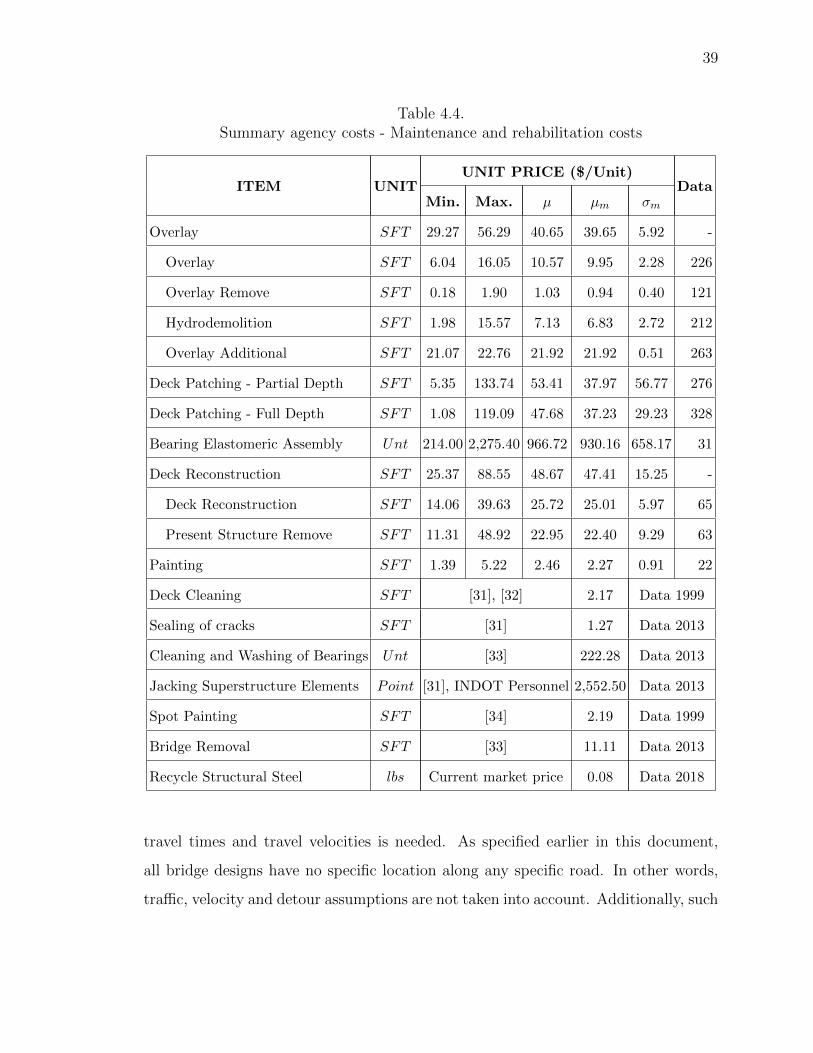
39

Table 4.4.Summary agency costs - Maintenance and rehabilitation costs

ITEM UNITUNIT PRICE ($/Unit)

DataMin. Max. µ µm σm

Overlay SFT 29.27 56.29 40.65 39.65 5.92 -

Overlay SFT 6.04 16.05 10.57 9.95 2.28 226

Overlay Remove SFT 0.18 1.90 1.03 0.94 0.40 121

Hydrodemolition SFT 1.98 15.57 7.13 6.83 2.72 212

Overlay Additional SFT 21.07 22.76 21.92 21.92 0.51 263

Deck Patching - Partial Depth SFT 5.35 133.74 53.41 37.97 56.77 276

Deck Patching - Full Depth SFT 1.08 119.09 47.68 37.23 29.23 328

Bearing Elastomeric Assembly Unt 214.00 2,275.40 966.72 930.16 658.17 31

Deck Reconstruction SFT 25.37 88.55 48.67 47.41 15.25 -

Deck Reconstruction SFT 14.06 39.63 25.72 25.01 5.97 65

Present Structure Remove SFT 11.31 48.92 22.95 22.40 9.29 63

Painting SFT 1.39 5.22 2.46 2.27 0.91 22

Deck Cleaning SFT [31], [32] 2.17 Data 1999

Sealing of cracks SFT [31] 1.27 Data 2013

Cleaning and Washing of Bearings Unt [33] 222.28 Data 2013

Jacking Superstructure Elements Point [31], INDOT Personnel 2,552.50 Data 2013

Spot Painting SFT [34] 2.19 Data 1999

Bridge Removal SFT [33] 11.11 Data 2013

Recycle Structural Steel lbs Current market price 0.08 Data 2018

travel times and travel velocities is needed. As specified earlier in this document,

all bridge designs have no specific location along any specific road. In other words,

traffic, velocity and detour assumptions are not taken into account. Additionally, such

40

assumptions are considered an oversimplification of the problem and could impact

negatively the outcome of the LCC comparison. More information about user costs

models can be found in Hawk [1] and Sinha et al. [20].

4.6 Probability Distribution Selection

In order to properly perform a Monte Carlo simulation, probability distributions

for different pay items are needed. Basic concepts of probability needed to under-

stand this process along with definitions, probability density functions and cumulative

density functions of every distribution used herein are presented in Appendix B.

The usage of historical data as a mean to capture the inherent stochastic nature

of different phenomena is a common practice. This can be accomplished by obtaining

the probability distribution of such events. It is true that for mathematical simplicity

simpler distributions like the normal distribution and the lognormal distribution, are

preferable. Also, due to lack of available data other distributions like the triangular

distribution and the PERT distribution could be useful, simplifying greatly the process

[35].

However, when the shape of the distribution is important, especially when histor-

ical sample data are available, consideration of multiple distribution to fit the data is

desirable. When two or more distributions appear to be plausible, certain statistical

test can be used to discriminate the relative validity of those. These tests are known

as goodness-of-fit tests for distributions. There are multiple techniques that can be

used including: the Akaike information criterion (AIC), the Bayesian information

criterion (BIC), the Chi-squared test (χ2), the Kolmogorov-Smirnov test (K-S) and

the Anderson-Darling test (A-D). Among them, the first two are the more mathe-

matically complex, while the last two are based on the comparison of the empirical

cumulative density function (ECDF) of the sample and the cumulative density func-

tion (CDF) of the assumed distribution. The A-D test is particularly useful when the

tails of a distribution are important [36]. The last three tests mentioned, as noted

41

by Ang and Tang [36]: “should be used only to help verify the validity of a theoret-

ical model that has been selected on the basis of other prior considerations, such as

through the application of appropriate probability papers, or even visual inspection

of an appropriate probability density function (PDF) with the available histogram”.

In light of this statement, the method used herein includes not only the use of the

K-S and A-D test for PDF selection but also an adequate visual inspection.

4.6.1 Kormogorov-Smirnov (K-S) test for goodness of fit

The general purpose of the test is to compare the ECDF with the CDF of the

tested theoretical distribution. The test acceptance is given by contrasting of the

maximum discrepancy between the ECDF and the CDF (Dn, given by the equation

4.8 and represented in Figure 4.2) and the critical limit value (Dαn) depending on the

desired significance level α. The distribution is considered as acceptable if Dn is less

than Dαn .

Dn = maxx| F (x)− Fn(x) | (4.8)

The critical value Dαn is defined for a particular significance level α by:

P (Dn ≤ Dαn) = 1− α (4.9)

Values for different significance levels can be consulted in different texts [36],

however for a 5% significance level (α = 0.05) and sets of more than 50 data points,

the critical value can be computed as:

Dαn =

1.36√n

(4.10)

42

Fig. 4.2. ECDF (Fn(x)) vs CDF (F (x)), K-S test parameter Dn forBox Beams unit price

4.6.2 Anderson-Darling (A-D) test for goodness of fit

This test was first proposed by Anderson and Darling in 1954 [37] and is focused

in placing more weight on the tails of the distribution. The calculation of the A-D

statistic is as follows:

A2 = −n− 1

n

n∑j=1

(2j − 1)[log uj + log (1− un−j+1)] (4.11)

then, an adjusted test statistic (A∗) and the critical value (cα) corresponding to

the desired significance level (in this case α = 0.05) is computed. Values for such

parameters depends on the type of distribution that is tested, for which tabulated

values can be consulted [36]. Most software includes the estimation of this value

within their routines. For this research Matlab R©is used for both the K-S and the

A-D tests.

43

4.6.3 PDF selection example

As described before, a proper PDF selections is based not only on the test statistic

but also on adequate visual inspection. The pay item chosen for a general explanation

of the process followed is the bridge concrete, specified as “Concrete Type C”. There

are 353 values found in the historic contractor database mentioned earlier in this

document. The general process is the following:

i . The number of bins used for the histogram based on the Doane’s formula,

which is a variation of the Sturge’s formula that attempsts to improve the

performance with non-normal data, is computed as follows:

k = 1 + log2 n+ log2

(1 +| g1 |σg1

)(4.12)

σg1 =

√6(n− 2)

(n+ 1)(n+ 3)(4.13)

where k is the number of bins needed (k = 13), n is the number of values

(n = 353) and g1 is the skewness of the data (g1 = 0.71).

ii . The histogram representing the data is plotted alongside with all the PDF’s

that are tested (see Figure 4.3(a)). The selection of the distributions to be

tested is based solely on a visual inspection (i.e. based on the histogram shape,

the distributions are selected among the wide variety available). In this case,

and for all the pay items analyzed, the selected distributions are: Normal dis-

tribution, Lognormal distribution, Gamma distribution, Logistic distribution,

Weibull distribution and Inverse Gaussian distribution. Appendix B presents

the PDF’s and the CDF’s of all the distributions used in this document.

iii . K-S and A-D tests are used in order to rank the goodness of fit of each distri-

bution. If more than one distribution is considered as a good fit for the historical

data, the lowest value of the Dn statistic and the A∗ statistic is selected. This

process is presented in Table 4.5. The values of Logical K-S and Logical A-D

44

CONCRETE TYPE C

Gamma Dist p= 0.1

100 200 300 400 500 600

Unit Cost ($/yd3)

0

0.5

1

1.5

2

2.5

3

3.5

4

4.510-3

DataNormalGammaWeibullLogNormalLogisticInv Gaussian

(a) Histogram and PDF’s tested

0 100 200 300 400 500 600 700 800

Quantiles of gamma Distribution

0

100

200

300

400

500

600

700

800

Qua

ntile

s of

Inpu

t Sam

ple

QQ Plot of Sample Data versus Distribution

(b) Q-Q plot - Selected PDF

0 100 200 300 400 500 600

Unit Cost ($/yd3)

0

0.1

0.2

0.3

0.4

0.5

0.6

0.7

0.8

0.9

1

Den

sity

Survivor Function

EmpiricalGamma

(c) Survival Function - Selected PDF

0 100 200 300 400 500 600

Unit Cost ($/yd3)

0

0.1

0.2

0.3

0.4

0.5

0.6

0.7

0.8

0.9

1

Den

sity

Cumulative Density Funtion

Data ECDFGamma CDF

(d) CDF - Selected PDF

Fig. 4.3. Graphical PDF Selection results - Pay item: Concrete Type C

represents the hypothesis test results as a logical value, where 0 indicates the

failure to reject the null hypothesis (i.e. the data can be represented with the

tested distribution), and 1 indicates the rejection of the null hypothesis. The

table also presents the p-value and the limiting values for both the K-S and A-D

tests, Dαn and cα respectively.

iv . In order to properly select the adequate distribution, both test are considered.

Then, a weight is given to each distribution depending on its ranked position

for each, the K-S and the A-D tests. Numeric values from 1 to 6 are given in

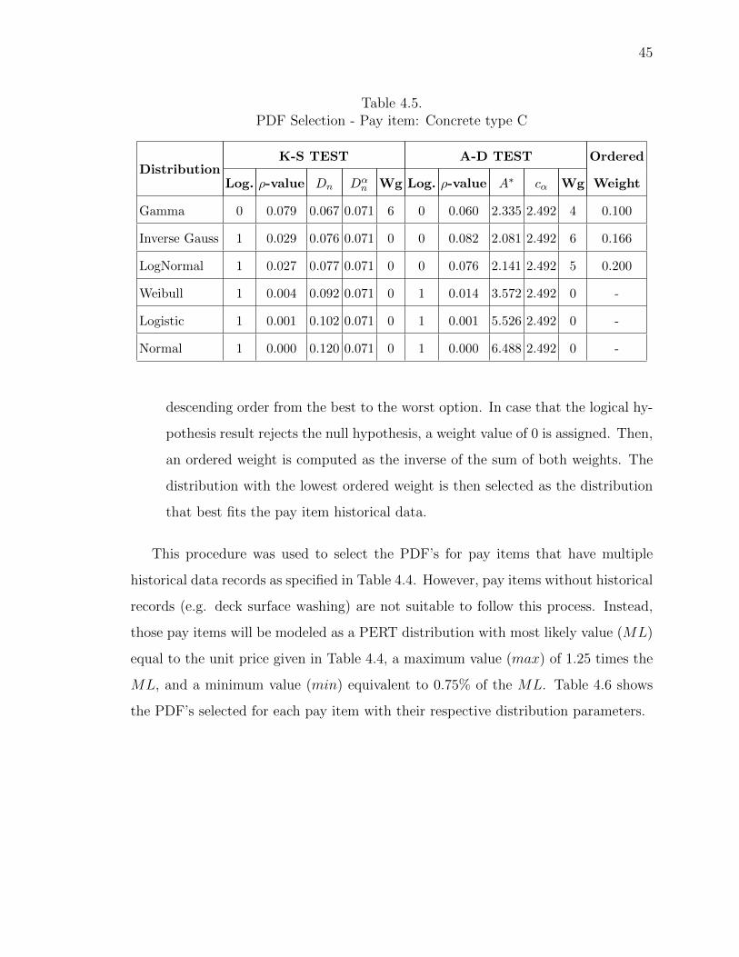
45

Table 4.5.PDF Selection - Pay item: Concrete type C

DistributionK-S TEST A-D TEST Ordered

Log. ρ-value Dn Dαn Wg Log. ρ-value A∗ cα Wg Weight

Gamma 0 0.079 0.067 0.071 6 0 0.060 2.335 2.492 4 0.100

Inverse Gauss 1 0.029 0.076 0.071 0 0 0.082 2.081 2.492 6 0.166

LogNormal 1 0.027 0.077 0.071 0 0 0.076 2.141 2.492 5 0.200

Weibull 1 0.004 0.092 0.071 0 1 0.014 3.572 2.492 0 -

Logistic 1 0.001 0.102 0.071 0 1 0.001 5.526 2.492 0 -

Normal 1 0.000 0.120 0.071 0 1 0.000 6.488 2.492 0 -

descending order from the best to the worst option. In case that the logical hy-

pothesis result rejects the null hypothesis, a weight value of 0 is assigned. Then,

an ordered weight is computed as the inverse of the sum of both weights. The

distribution with the lowest ordered weight is then selected as the distribution

that best fits the pay item historical data.

This procedure was used to select the PDF’s for pay items that have multiple

historical data records as specified in Table 4.4. However, pay items without historical

records (e.g. deck surface washing) are not suitable to follow this process. Instead,

those pay items will be modeled as a PERT distribution with most likely value (ML)

equal to the unit price given in Table 4.4, a maximum value (max) of 1.25 times the

ML, and a minimum value (min) equivalent to 0.75% of the ML. Table 4.6 shows

the PDF’s selected for each pay item with their respective distribution parameters.

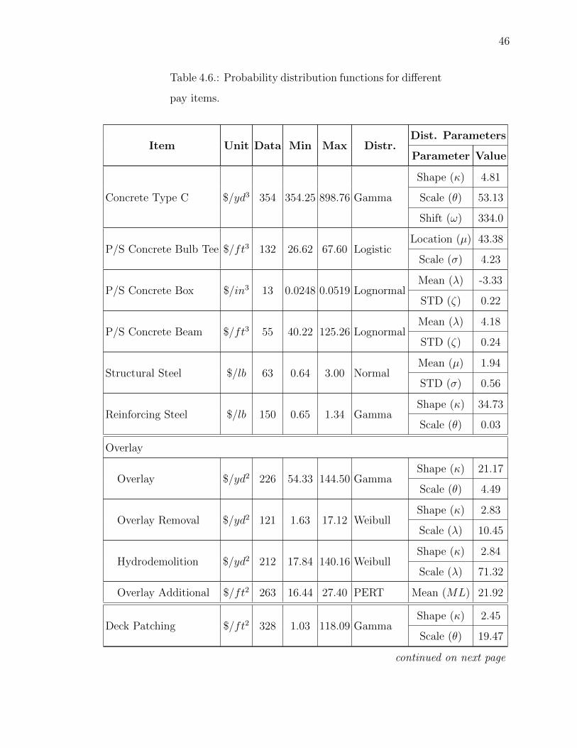
46

Table 4.6.: Probability distribution functions for different

pay items.

Item Unit Data Min Max Distr.Dist. Parameters

Parameter Value

Concrete Type C $/yd3 354 354.25 898.76 Gamma

Shape (κ) 4.81

Scale (θ) 53.13

Shift (ω) 334.0

P/S Concrete Bulb Tee $/ft3 132 26.62 67.60 LogisticLocation (µ) 43.38

Scale (σ) 4.23

P/S Concrete Box $/in3 13 0.0248 0.0519 LognormalMean (λ) -3.33

STD (ζ) 0.22

P/S Concrete Beam $/ft3 55 40.22 125.26 LognormalMean (λ) 4.18

STD (ζ) 0.24

Structural Steel $/lb 63 0.64 3.00 NormalMean (µ) 1.94

STD (σ) 0.56

Reinforcing Steel $/lb 150 0.65 1.34 GammaShape (κ) 34.73

Scale (θ) 0.03

Overlay

Overlay $/yd2 226 54.33 144.50 GammaShape (κ) 21.17

Scale (θ) 4.49

Overlay Removal $/yd2 121 1.63 17.12 WeibullShape (κ) 2.83

Scale (λ) 10.45

Hydrodemolition $/yd2 212 17.84 140.16 WeibullShape (κ) 2.84

Scale (λ) 71.32

Overlay Additional $/ft2 263 16.44 27.40 PERT Mean (ML) 21.92

Deck Patching $/ft2 328 1.03 118.09 GammaShape (κ) 2.45

Scale (θ) 19.47

continued on next page

47

Table 4.6.: continued

Item Unit Data Min Max Distr.Dist. Parameters

Parameter Value

Bearing Assembly $/unt 31 214.00 2,275 LognormalMean (λ) 6.65

STD (ζ) 0.72

Painting $/ft2 22 1.39 5.22 LognormalMean (λ) 0.83

STD (ζ) 0.41

Deck Cleaning $/ft2 - 1.63 2.71 PERT Mean (ML) 2.17

Sealing of cracks $/ft2 - 0.95 1.59 PERT Mean (ML) 1.27

Jacking $/unt - 1,914 3,190 PERT Mean (ML) 2,553

Bridge Removal $/ft2 - 8.33 13.89 PERT Mean (ML) 11.11

Deck Reconstruction

Deck Reconstruction $/yd3 65 379.59 1,070 Inv. GaussMean (µ) 695

Shape (λ) 12,683

Structure Removal $/ft2 63 1.39 5.22 LognormalMean (λ) 3.05

STD (ζ) 0.38

Spot Painting $/ft2 - 1.64 2.74 PERT Mean (ML) 2.19

Recycle Struc. Steel $/lb - 0.06 0.10 PERT Mean (ML) 0.08

Galvanizing $/ft2 - 0.22 0.36 PERT Mean (ML) 0.29

Discount rate % - 2.00 6.00 PERT Mean (ML) 4.00

Finally, some PDF’s have heavier tails than others, which means that when a

simulation uses a random number generator those values could be easily chosen for

a number of iterations. However, according to the historical data, extreme values

are unlikely to happen. Consequently, for simulation purposes only, a range between

0.75 times the minimum value and 1.25 times the maximum value was used. Values

outside these boundaries were taken as the 0.75 times the minimum and 1.25 times

the maximum values, respectively.

48

5. DETERIORATION MODELS FOR INDIANA BRIDGES

Deterioration curves are critical for development of the BLCCA. Their accurate de-

termination will lead to more precise answers and better recommendations to de-

signers. The use of the NBI database to develop deterioration curves is the most

commonly utilized practice. Since this study is focused only on the Indiana bridge

system administrated by INDOT, deterioration curves will consider the Indiana NBI

database. Accordingly, deterioration curves made for the Indiana state highway sys-

tem by Moomen et al. [17], Sinha et al. [20] and Cha et al. [38] will be used.

In addition to the deterioration path for each material type, a limiting condition

rating needs to be chosen in order to establish the lowest allowed bound of deteriora-

tion. This lower bound could vary depending on the budget allocation and availability.

According to INDOT experience, the threshold for the state of Indiana is 4. Addi-

tionally, analyzing the historical NBI database it is clear that a condition rating of 4

is considered as the lowest deterioration limit before a major rehab or repair action

is scheduled. Consequently, for this research a condition rating of 4 is established as

the threshold before a major work action is needed.

Nonetheless, it is important to mention that there are some drawbacks related

to the use of the NBI condition ratings. First, these are based on visual inspections

which involves a variability between consecutive inspections. Since these inspections

are inherently subjective, the usage of those needs to be done carefully. Second, and

as it can be seen in Figure 5.1 there are condition ratings that are physically unlikely

for the bridge age that is provided. For instance, there are records that indicates that

a bridge could be a condition 9 (excellent condition) even for bridge ages older than

30 years, which is not likely. These abnormal records could be explained not only with

the variability due to the visual inspection but also with the lack of historical records

of maintenance, rehabilitation or reconstruction procedures for existing bridges that

49

can be found in the database. As a result, the deterioration curves obtained from

those records need to be treated carefully and with engineering judgment.

Deterioration rates vary depending on the database and method used to compute

it. Nonetheless, it is clear that deterioration rate is time dependent. Focusing on

steel structures only as shown in Figure 5.1, Moomen et al. [17] predicted that a

steel bridge deteriorates to a replacement state in less than 50 years. In contrast,

the constant deterioration rate used by Cha et al. [38] projected an age close to 90

years, while the deterioration curve used by Sinha et al. [20] for the Indiana Bridge

Management System (IBMS) stated that this life value is in the vicinity of 80 years

for the same threshold rating. Steel superstructure deterioration curves used in the

IBMS appear to fit better the historical data.

Fig. 5.1. Deterioration curves example for steel bridges.

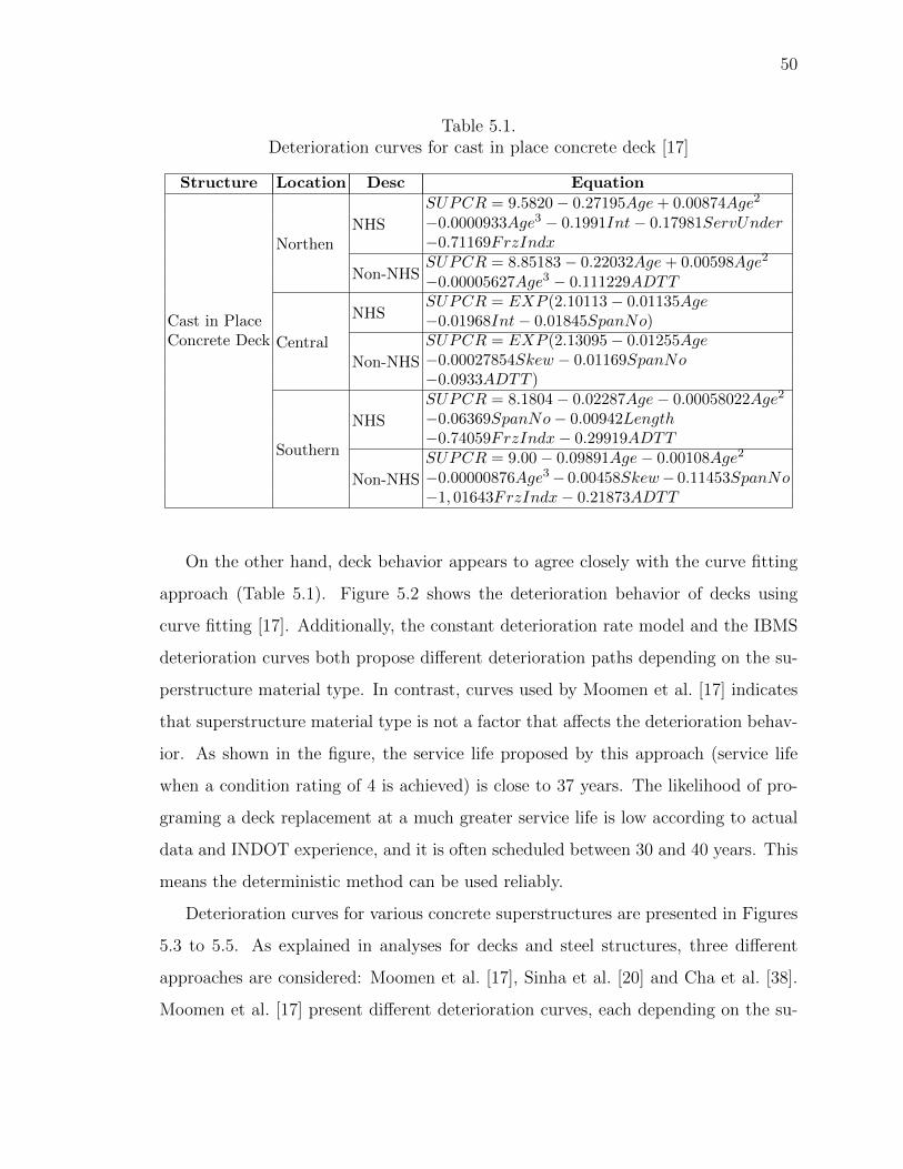
50

Table 5.1.Deterioration curves for cast in place concrete deck [17]

Structure Location Desc Equation

NorthenNHS

SUPCR = 9.5820− 0.27195Age+ 0.00874Age2

−0.0000933Age3 − 0.1991Int− 0.17981ServUnder−0.71169FrzIndx

Non-NHSSUPCR = 8.85183− 0.22032Age+ 0.00598Age2

−0.00005627Age3 − 0.111229ADTT

Central

NHSSUPCR = EXP (2.10113− 0.01135Age

Cast in Place −0.01968Int− 0.01845SpanNo)Concrete Deck

Non-NHS

SUPCR = EXP (2.13095− 0.01255Age−0.00027854Skew − 0.01169SpanNo−0.0933ADTT )

Southern

NHS

SUPCR = 8.1804− 0.02287Age− 0.00058022Age2

−0.06369SpanNo− 0.00942Length−0.74059FrzIndx− 0.29919ADTT

Non-NHS

SUPCR = 9.00− 0.09891Age− 0.00108Age2

−0.00000876Age3− 0.00458Skew− 0.11453SpanNo−1, 01643FrzIndx− 0.21873ADTT

On the other hand, deck behavior appears to agree closely with the curve fitting

approach (Table 5.1). Figure 5.2 shows the deterioration behavior of decks using

curve fitting [17]. Additionally, the constant deterioration rate model and the IBMS

deterioration curves both propose different deterioration paths depending on the su-

perstructure material type. In contrast, curves used by Moomen et al. [17] indicates

that superstructure material type is not a factor that affects the deterioration behav-

ior. As shown in the figure, the service life proposed by this approach (service life

when a condition rating of 4 is achieved) is close to 37 years. The likelihood of pro-

graming a deck replacement at a much greater service life is low according to actual

data and INDOT experience, and it is often scheduled between 30 and 40 years. This

means the deterministic method can be used reliably.

Deterioration curves for various concrete superstructures are presented in Figures

5.3 to 5.5. As explained in analyses for decks and steel structures, three different

approaches are considered: Moomen et al. [17], Sinha et al. [20] and Cha et al. [38].

Moomen et al. [17] present different deterioration curves, each depending on the su-

51

perstructure structural type. However, threshold rating age for different structural

types lies between 55 and 65 years not only for the curve fitting approach but also for

the constant deterioration rate method [38]. In contrast, IBMS deterioration curve

reaches a condition rating of 4 at 80 years. INDOT experience indicates that is

unlikely to have a concrete superstructure older than 70 years without any rehabil-

itation or repair. Deterioration models proposed by Moomen et al. [17], appear to

better reflect the common practices in Indiana for concrete superstructures.

Fig. 5.2. Deck deterioration example.

Deterioration curves are used to predict maintenance, rehabilitation and recon-

struction scheduling for each of the design options considered. For concrete structures,

models proposed by Moomen et al. [17] were selected. Additionally, the model for

steel structures corresponds to curves proposed by Sinha et al. [20]. Once an ele-

ment reaches the threshold for each condition, a jump in the condition rating will

be assumed and the deterioration afterwards will follow the correspondent curve (see

Figure 2.3). Final deterioration profiles were used to allocate agency and user costs

during the BLCCA process.

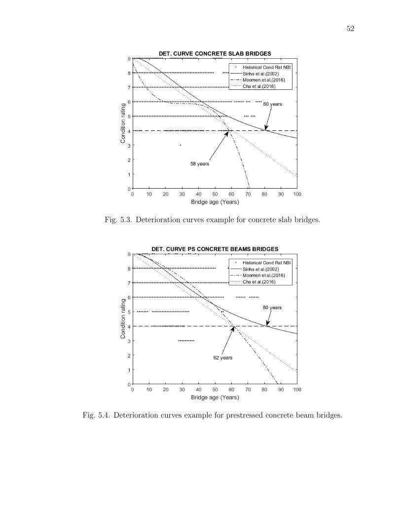
52

Fig. 5.3. Deterioration curves example for concrete slab bridges.

Fig. 5.4. Deterioration curves example for prestressed concrete beam bridges.

53

Fig. 5.5. Deterioration curves example for prestressed concrete box bridges.

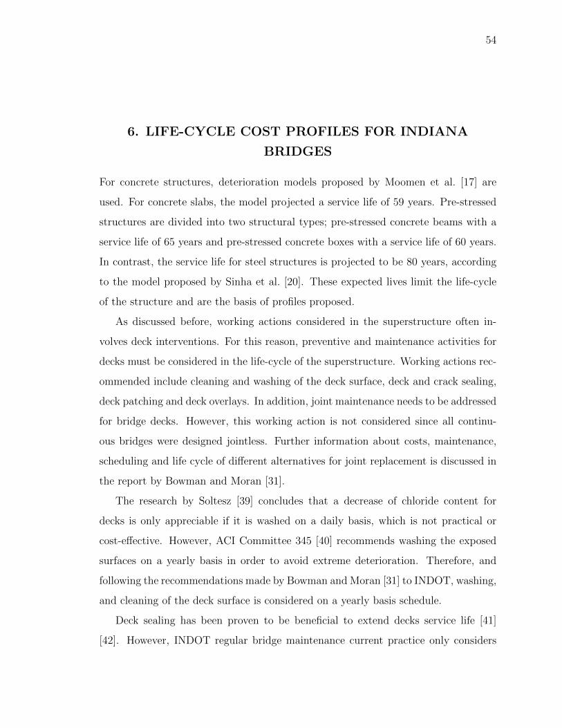
54

6. LIFE-CYCLE COST PROFILES FOR INDIANA

BRIDGES

For concrete structures, deterioration models proposed by Moomen et al. [17] are

used. For concrete slabs, the model projected a service life of 59 years. Pre-stressed

structures are divided into two structural types; pre-stressed concrete beams with a

service life of 65 years and pre-stressed concrete boxes with a service life of 60 years.

In contrast, the service life for steel structures is projected to be 80 years, according

to the model proposed by Sinha et al. [20]. These expected lives limit the life-cycle

of the structure and are the basis of profiles proposed.

As discussed before, working actions considered in the superstructure often in-

volves deck interventions. For this reason, preventive and maintenance activities for

decks must be considered in the life-cycle of the superstructure. Working actions rec-

ommended include cleaning and washing of the deck surface, deck and crack sealing,

deck patching and deck overlays. In addition, joint maintenance needs to be addressed

for bridge decks. However, this working action is not considered since all continu-

ous bridges were designed jointless. Further information about costs, maintenance,

scheduling and life cycle of different alternatives for joint replacement is discussed in

the report by Bowman and Moran [31].

The research by Soltesz [39] concludes that a decrease of chloride content for

decks is only appreciable if it is washed on a daily basis, which is not practical or

cost-effective. However, ACI Committee 345 [40] recommends washing the exposed

surfaces on a yearly basis in order to avoid extreme deterioration. Therefore, and

following the recommendations made by Bowman and Moran [31] to INDOT, washing,

and cleaning of the deck surface is considered on a yearly basis schedule.

Deck sealing has been proven to be beneficial to extend decks service life [41]

[42]. However, INDOT regular bridge maintenance current practice only considers

55

it during deck construction or reconstruction [31]. Soriano [43] and Mamaghani et

al. [44] stated that the first sealing process should be done within 3 to 6 months

after construction, with justification to consider it at year 0 or simultaneously with

deck reconstructions. Regular use of sealants could extend the initial life of a deck

up to 40 years according to Zemajtis and Weyers [45]. However, sealants depending

on the fabricator, weather conditions, and traffic wearing have different service lives.

Sealant service life expectancy varies from 5 to 10 years (based on studies made by

Weyers et al. [46], Zemajtis and Weyers [45], Meggers [47], Soriano [43], Mamaghani et

al. [44], Wenzlick [48] and ACI Commitie 345 [40]) and need to be replaced routinely.

Both Bowman and Moran [31], and Frosch et al. [41] [42] recommended that Indiana

bridge decks to be resealed every 5 years for high traffic roads. Consequently, profiles

considering deck sealing every 5 years and a deck overlay after 40 years are considered.

Concrete deck patching involves the removal of contaminated concrete down to

the level of the reinforcement steel in the affected area, followed by steel cleaning and

replacement if necessary, and installation of the final patch with new high-quality con-

crete or mortar with low permeability [49]. There are some disadvantages using this

method that are related mostly to the incomplete or insufficient removal of concrete

in the affected area. In Indiana, some decks have experienced significant corrosion

processes after only 7 years from the reparation according to Olek and Liu [49]. This

repair action must be performed as early as possible in order to avoid accelerated

corrosion problems. Bowman and Moran [31] proposed a 10 year life cycle for patch-

ing repairs for bridge decks areas with no more than 10% of the total deck surface

repaired. Additionally, as considered by Weyers et al. [46] in their proposed life-cycle

models, an increase in maintenance cost due to progressive deterioration needs to be

considered.

Among the numerous deck protection systems that are available, overlays are

considered as one of the most cost-effective options since the early 80’s [50]. There are

different types of overlays: portland cement overlays, polymer, and epoxy mortars or

concretes and polymer impregnated concrete [51]. As noted by Frosch and Blackman

56

[52] Portland cement overlays include low-slump dense concrete (LSDC), polymer-

modified concrete (also called latex-modified concrete) and fiber-reinforced concrete

(FRC). Latex modified concrete overlays are the most common type found in Indiana.

Polymer-impregnated concrete overlays will not be discussed in this report as they

have not become generally effective, economical, or practical [51]. Asphaltic concrete

overlays are relatively porous and, by themselves, do not provide an effective seal.

This porosity entraps salt-laden moisture which, in the absence of an effective deck

sealer, can promote deck deterioration [40]). The current INDOT policy considers

the service life of the deck surface to be between 20 or 25 years, followed by a deck

re-placement after 15 to 20 years [31]. This policy does not include deck maintenance

activities. To conclude, latex modified concrete overlays after 25 years of bridge

construction followed by deck reconstruction after 20 years is considered. The service

life of over-lays after a bridge repair activity will be considered as 20 years as a lower

bound.

Maintenance activities on the superstructure vary depending on the material type

and in some cases on the structural type chosen. There are some activities that can be

considered as common regarding those two characteristics. Bearing maintenance and

replacement is one of them. Different bearing types are available such as elastomeric

bearings, cotton duck pads, sliding bearing, manufactured high load multi-rotational

bearings and mechanical steel bearings among others [53]. However, INDOT generally

only uses two types of devices: for concrete members elastomeric pad devices, and for

steel structures elastomeric and steel bearings [54]. This research only will consider

elastomeric devices as a common bearing type for all structural designs. Preventive

maintenance activities such as cleaning, washing, and flushing are commonly used for

elastomeric bearings on a biannual basis [31].

The service life of elastomeric devices when they are well maintained, constructed

and designed can last as long as the structure [55] [53]. However, in order to achieve

a service life of 100-plus-years, more emphasis must be placed on manufacturing

quality [53]. Aria and Akbari [56] proposed a service life between 30 to 50 years,

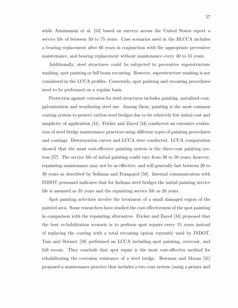
57

while Azizinamini et al. [53] based on surveys across the United States report a

service life of between 50 to 75 years. Case scenarios used in the BLCCA includes

a bearing replacement after 60 years in conjunction with the appropriate preventive

maintenance, and bearing replacement without maintenance every 40 to 55 years.

Additionally, steel structures could be subjected to preventive superstructure

washing, spot painting or full beam recoating. However, superstructure washing is not

considered in the LCCA profiles. Conversely, spot painting and recoating procedures

need to be performed on a regular basis.

Protection against corrosion for steel structures includes painting, metalized coat,

galvanization and weathering steel use. Among them, painting is the most common

coating system to protect carbon steel bridges due to its relatively low initial cost and

simplicity of application [31]. Fricker and Zayed [34] conducted an extensive evalua-

tion of steel bridge maintenance practices using different types of painting procedures

and coatings. Deterioration curves and LCCA were conducted. LCCA computation

showed that the most cost-effective painting system is the three-coat painting sys-

tem [57]. The service life of initial painting could vary from 30 to 50 years, however,

repainting maintenance may not be as effective, and will generally last between 20 to

30 years as described by Soliman and Frangopol [58]. Internal communication with

INDOT personnel indicates that for Indiana steel bridges the initial painting service

life is assumed as 35 years and the repainting service life as 20 years.

Spot painting activities involve the treatment of a small damaged region of the

painted area. Some researchers have studied the cost-effectiveness of the spot painting

in comparison with the repainting alternative. Fricker and Zayed [34] proposed that

the best re-habilitation scenario is to perform spot repairs every 15 years instead

of replacing the coating with a total recoating option currently used by INDOT.

Tam and Stiemer [59] performed an LCCA including spot painting, overcoat, and

full recoat. They conclude that spot repair is the most cost-effective method for

rehabilitating the corrosion resistance of a steel bridge. Bowman and Moran [31]

proposed a maintenance practice that includes a two coat system (using a primer and

58

a top coat) as part of spot painting that is performed every 10 years in areas not

larger than 10% of the exposed area.

No extension in the service life of the different superstructures was assumed as a

result of different maintenance and preventive working actions. There is not historical

data to support such assumption into the analysis. The combination of different

working actions as described before, and its application to a given structure, leads

to a unique life-cycle profile. Different alternatives were considered for each of the

superstructure types analyzed, leading to the optimal life-cycle profiles for each one of

them based on lower present values computed using BLCCA. All the life-cycle profiles

considered are presented in Appendix C. Several different profiles were chosen to

compare cost effectiveness and are illustrated as follows:

• Slab bridges (see Figure 6.1). Cleaning and washing as a regular annual activity.

Cleaning and deck sealing every 5 years following bridge construction. A deck

overlay at 40 years. Finally, a bridge superstructure replacement at the end of

its service life (58 years).

Fig. 6.1. Life-cycle profile for slab bridges.

• Prestressed concrete I beams with elastomeric bearings (see Figure 6.2). Clean-

ing and washing of the deck as a regular annual activity. Cleaning and deck

sealing every 5 years following bridge construction. A full deck replacement

59

at 40 years along with bearing replacements. Finally, a bridge superstructure

replacement at the end of its service life (65 years).

Fig. 6.2. Life-cycle profile for prestressed concrete I beams with elas-tomeric bearings.

• Pre-stressed concrete box beams (see Figure 6.3). Cleaning and washing of

the deck as a regular annual activity. Cleaning and deck sealing every 5 years

following bridge construction. A full deck replacement at 40 years along with

bearings replacements. Finally, a bridge superstructure replacement at the end

of its service life (60 years).

• Steel superstructures (see Figure 6.4). Cleaning and washing of the deck as a

regular annual activity. Cleaning and deck sealing every 5 years following bridge

construction. One bearings replacement at 40 years. A full deck replacement at

40 years. Spot painting every 10 years on less than 10% of the exposed beam

area. Finally, a bridge superstructure replacement at the end of its service life

(80 years).

Through discussion with INDOT personnel, it was noted that accelerated deteri-

oration at beams ends is one of the main reasons of why prestressed elements show

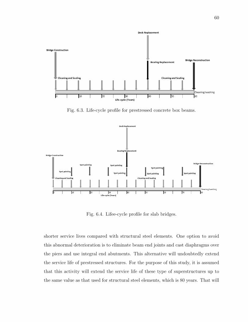
60

Fig. 6.3. Life-cycle profile for prestressed concrete box beams.

Fig. 6.4. Lifee-cycle profile for slab bridges.

shorter service lives compared with structural steel elements. One option to avoid

this abnormal deterioration is to eliminate beam end joints and cast diaphragms over

the piers and use integral end abutments. This alternative will undoubtedly extend

the service life of prestressed structures. For the purpose of this study, it is assumed

that this activity will extend the service life of these type of superstructures up to

the same value as that used for structural steel elements, which is 80 years. That will

61

effectively represent and is an extension of 15 years of the service life. Therefore, life

cycle profiles including this improvement are also considered, adding the correspond-

ing diaphragm initial cost to the alternative analyzed. In addition, SDCL system

service life is also extended in the same proportion since the system itself is based on

the same principle of integral abutments and intermediate pier diaphragms, making

its service life 95 years. Consequently, profiles chosen to compare its cost effectiveness

are the following:

• Steel superstructures SDCL (see Figure 6.5). Cleaning and washing of the deck

as a regular annual activity. Cleaning and deck sealing every 5 years following

bridge construction. A full deck replacement at 50 years. Spot painting every 10

years less than 10% of the exposed beam area. Finally, a bridge superstructure

replacement at the end of its service life (95 years).

Fig. 6.5. Life-cycle profile for steel structures SDCL.

• Prestressed concrete I beams including diaphragms (see Figure 6.6). Cleaning

and washing of the deck as a regular annual activity. Cleaning and deck sealing

every 5 years following bridge construction. A full deck replacement at 40

years. Finally, a bridge superstructure replacement at the end of its service life

(80 years).

Finally, section loss due to corrosion for steel superstructures is considered as one

of the main reasons for deterioration. Therefore, corrosion protection is important

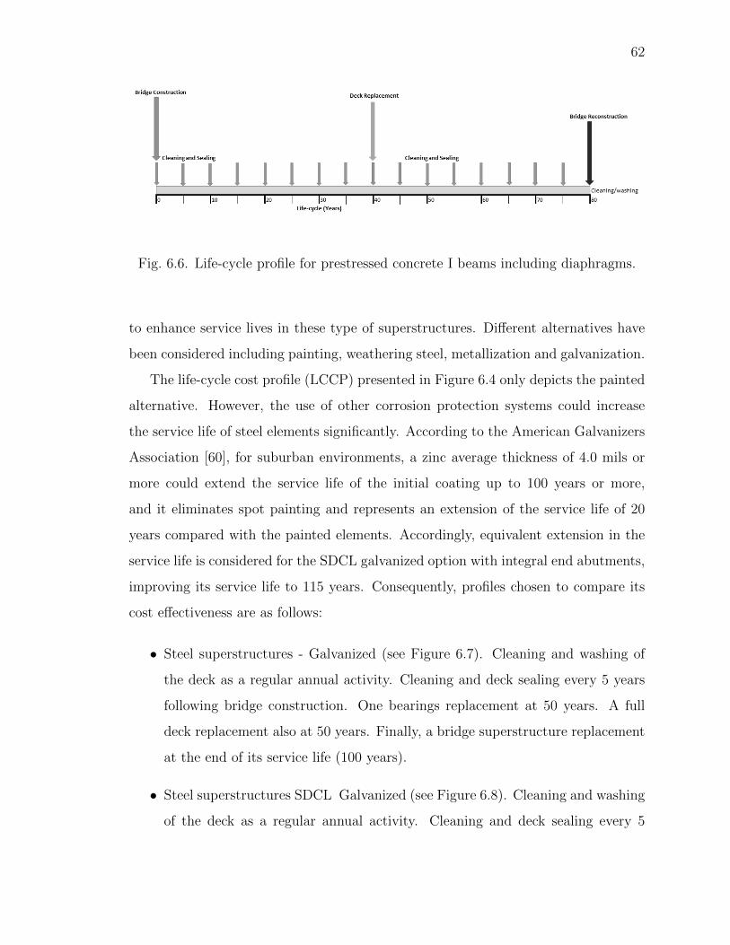
62

Fig. 6.6. Life-cycle profile for prestressed concrete I beams including diaphragms.

to enhance service lives in these type of superstructures. Different alternatives have

been considered including painting, weathering steel, metallization and galvanization.

The life-cycle cost profile (LCCP) presented in Figure 6.4 only depicts the painted

alternative. However, the use of other corrosion protection systems could increase

the service life of steel elements significantly. According to the American Galvanizers

Association [60], for suburban environments, a zinc average thickness of 4.0 mils or

more could extend the service life of the initial coating up to 100 years or more,

and it eliminates spot painting and represents an extension of the service life of 20

years compared with the painted elements. Accordingly, equivalent extension in the

service life is considered for the SDCL galvanized option with integral end abutments,

improving its service life to 115 years. Consequently, profiles chosen to compare its

cost effectiveness are as follows:

• Steel superstructures - Galvanized (see Figure 6.7). Cleaning and washing of

the deck as a regular annual activity. Cleaning and deck sealing every 5 years

following bridge construction. One bearings replacement at 50 years. A full

deck replacement also at 50 years. Finally, a bridge superstructure replacement

at the end of its service life (100 years).

• Steel superstructures SDCL Galvanized (see Figure 6.8). Cleaning and washing

of the deck as a regular annual activity. Cleaning and deck sealing every 5

63

Fig. 6.7. Life-cycle profile for galvanized steel structures.

years following bridge construction. Full deck replacements at 40 and 80 years.

Finally, a bridge superstructure replacement at the end of its service life (115

years).

Fig. 6.8. Life-cycle profile for galvanized steel structures SDCL.

It is important to mention that continuous steel galvanized beam structures with

integral end abutments are not considered in this study due to its cost-effectiveness.

As it can be seen in Chapter 7 results for the case of SDCL, if galvanized and painted

options are compared, the extension in service life due to galvanization involves an

additional deck reconstruction, that impact negatively the cost effectiveness of this

alternative. Following this trend, it is assumed that the extension in the service life

due to the inclusion of integral end abutments for continuous steel galvanized struc-

64

tures will also require an additional deck reconstruction that will impact negatively

the final outcome of this alternative.

65

7. LIFE-CYCLE COST ANALYSIS FOR INDIANA

BRIDGES

Results of the bridge design, cost allocation, and deterioration curves were used to

create the BLCCA for each design option. Those investigations will be the starting

point for recommendations made to designers based on BLCCA.

Sinha et al. [20] developed a Life-Cycle Cost module for the Indiana bridge man-

agement system (IBMS) called LCCOST. The outcome of this module is the difference

in expected life-cycle costs with or without the decision tree module recommenda-

tion (maintenance / rehabilitation / reconstruction). Nevertheless, LCCOST does

not compare different alternatives for the same project in terms of life-cycle costs.

This study can be understood as a complementary tool for agencies rather than an

extension to the modules created for the IBMS.

Life cycle profiles indicate not only the possible location for each major and routine

working actions, but they also indicate the length of the life cycle itself. Depending

on the type of material, structural type and major work actions considered, the length

of the life cycle could vary. In order to compare different options using BLCCA, there

is a need to establish a comparable service life for all alternatives. If two alternatives

with different service lives are to be compared, the least common multiple of the two

estimated service lives of the two alternatives must be used according to Grant and

Grant-Ireson [61]. However, it is assumed that in the case of highway assets with

long service lives like bridges, it is likely to replace the structure in the same place

over and over again rather than replace it in different locations each time. This factor

implies that the life cycle is recurrent independent of the structure type used.

Consequently, it can be assumed that each alternative will be indefinitely replaced,

in other words in perpetuity. Fwa [62] and Ford et al. [63] both describe methods to

compute the present worth of life cycle cost in perpetuity. Equation 7.1 shows Ford‘s

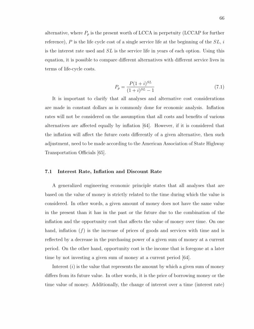
66

alternative, where Pp is the present worth of LCCA in perpetuity (LCCAP for further

reference), P is the life cycle cost of a single service life at the beginning of the SL, i

is the interest rate used and SL is the service life in years of each option. Using this

equation, it is possible to compare different alternatives with different service lives in

terms of life-cycle costs.

Pp =P (1 + i)SL

(1 + i)SL − 1(7.1)

It is important to clarify that all analyses and alternative cost considerations

are made in constant dollars as is commonly done for economic analysis. Inflation

rates will not be considered on the assumption that all costs and benefits of various

alternatives are affected equally by inflation [64]. However, if it is considered that

the inflation will affect the future costs differently of a given alternative, then such

adjustment, need to be made according to the American Association of State Highway

Transportation Officials [65].

7.1 Interest Rate, Inflation and Discount Rate

A generalized engineering economic principle states that all analyses that are

based on the value of money is strictly related to the time during which the value is

considered. In other words, a given amount of money does not have the same value

in the present than it has in the past or the future due to the combination of the

inflation and the opportunity cost that affects the value of money over time. On one

hand, inflation (f) is the increase of prices of goods and services with time and is

reflected by a decrease in the purchasing power of a given sum of money at a current

period. On the other hand, opportunity cost is the income that is foregone at a later

time by not investing a given sum of money at a current period [64].

Interest (i) is the value that represents the amount by which a given sum of money

differs from its future value. In other words, it is the price of borrowing money or the

time value of money. Additionally, the change of interest over a time (interest rate)

67

used to compute the present value of a future sum or cash flow is known as discount

rate (DR). By definition (see Equation 7.2), inflation has to be included when the

discount rate needs to be determined. However, and as specified before, it is assumed

that inflation will affect all costs the same, which is the reason why inflation is not

considered or taken as 0%.

DR =i− f1 + f

(7.2)

Discount rates differ depending on the economic activity analyzed. For instance,

the discount rate used for social analyses is often different than that used for highway

asset management. Some economist have suggested that the long-term true cost of

money to be between 4% and 6% [50]. The value often used for highway bridge

management according to the Indiana Department of Transportation is 4% [22] [31].

For the purposes of the stochastic simulation, the discount rate is modeled as a

Pert distribution with a most probable value of 4%, a minimum value of 2% and a

maximum value of 6%. Interest equations and equivalences for different cash flows

can be consulted in Appendix D.

7.2 Life-Cycle Cost Analysis Comparison

There are several criteria used to assess the economic efficiency of a project. Some

of them are listed as:

• Present worth of cost (PWC)

• Equivalent uniform annual cost (EUAC)

• Equivalent uniform annual return (EUAR)

• Net present value (NPV)

• Internal rate of return (IRR)

• Benefit-cost ratio (BCR)

68

The first two indicators of economic efficiency are applicable when all alternatives

have a similar expected level of benefits and cost minimization is the main objective

of the analysis. However, the alternatives analyzed in this document do not have the

same level of benefits, as demonstrated by the salvage value for each superstructure

type. The last two criteria require a solid estimation of the benefits resulting from the

implementation of the alternatives analyzed. Therefore, a complete socio-economic

analysis is needed. Such an analysis is outside of the scope of this project and requires

a specific location for the alternative chosen. Additionally, these two alternatives are

not used for comparing cost-differences in economic analyses. As a consequence,

EUAR and NPV are the most common indicators used. However, only NPV is the

approach used in this study because, for agency decision makers it is more useful to

know the cost upfront than the equivalent uniform annual cost for this specific case.

7.2.1 Equivalent uniform annual return (EUAR)

The EUAR is the combination of all costs and benefits expected from a project

expressed into a single annual value of return over the analysis period. This method

is useful when all the alternatives have different level of cost or benefits, or when the

analysis periods differ from one option to the other.

7.2.2 Net present value (NPV)

The NPV is understood as the difference between the present worth of benefits

and the present worth of costs. Basically, this method represents the value of the

project at the time of the base year of the analysis period or the year of the decision

making. NPV is often considered as the most appropriate of all economic efficiency

indicators because it provides a magnitude of net benefits in monetary terms [64].

Therefore, the alternative with the lowest NPV is considered the most economically

efficient. For the case of this study, costs are treated as positive values and benefits

as negative values. Consequently, the lowest value of NPV is desired.

69

7.3 Life-cycle cost analysis -Deterministc approach-

Initial cost comparison, as well as LCCA, were made for every superstructure

type considered. Table 7.1 presents a summary of the life-cycle cost analysis for

simply supported bridges with a simple span of 30-ft (detailed computation of this

values can be found in the example given in Appendix E). The discount rate used

for the life-cycle cost in perpetuity (LCCAP) is 4%. It presents the service life, total

life cycle cost (LCCA), LCCAP and the cost-effectiveness-ratio between the initial

cost and LCCAP of the different superstructure types (ERInitialCost and ERLCCAP ,

respectively). Ratios shown correspond to the ratio between the option analyzed

and the lowest price among all the alternatives for a given span length as shown in

Equation 7.3.

ERcost =CAlt

mini (CAlt1 , CAlt2 , . . . , CAlti)(7.3)

The results for the LCCA shown in Table 7.1 illustrate the evidence of considering

all costs for various structural types. The cost-effectiveness ratio for initial cost,

ERInitialCost, clearly shows that slab bridges provide the best alternative, with most

other systems costing an additional 15% or more. However, if the cost-effectiveness

ratio in perpetuity is examined, ERLCCAP , the results change notably. In this case

(for a 30-ft span) the slab bridge is still the most cost-effective solution, but the cost

differential - ERInitialCost versus ERLCCAP - changes significantly, with other systems

becoming more competitive. The four (4) beam and five (5) beam galvanized rolled

beam system have notably closed the cost gap. Other structural systems have also

improved in cost-effectiveness when all long-term costs are considered.

Figures 7.1 to 7.3 show the initial cost and LCCAP comparison for simply sup-

ported beams for all span ranges using the deterministic approach. As it can be seen

in the figures, in general the inclusion of long term-costs using LCCA reduces the

difference between all the alternatives for the same span length. Explicitly, for span

range 1, it is shown that the slab bridge is the most cost-effective solution either

70

Table 7.1.LCC summary example: simply supported beams -span length 30ft

TypeS L Initial Cost

ERInitialCostLCCA LCCAP

ERLCCAP(years) ($) ($) ($)

Slab Bridge 58 51,438 1.00 133,591 148,900 1.00

Prestressed Concrete

65 59,747 1.16 157,199 170,522 1.15AASHTO BeamsBearings


80 73,639 1.43 164,639 172,106 1.16AASHTO BeamsDiaphragms


60 75,404 1.47 170,217 188,097 1.26Concrete BoxBeams

Structural Steel

80 59,224 1.15 157,248 164,380 1.10Beams Painted4 beams

Structural Steel

80 59,464 1.16 158,535 165,725 1.11Beams Painted5 beams

Structural Steel

100 62,234 1.21 154,594 157,717 1.06Beams Galvanized4 beams

Structural Steel

100 62,511 1.22 155,573 158,715 1.07Beams Galvanized5 beams

Structural Steel

100 62,790 1.22 155,139 158,272 1.06FPG Galvanized4 beams

Structural Steel

100 67,921 1.32 161,332 164,591 1.11FPG Galvanized6 beams

considering or not considering long-term costs for spans less than 45-ft. However, for

spans longer than 45-ft, the inclusion of galvanized steel structures specifically the

four (4) beam configuration is the most cost-effective alternative. In contrast, if only

initial costs are considered, painted rolled beams and prestressed concrete AASHTO

beams would be the preferable options. Additionally, it is important to mention that

71

the FPG option is among the cost-effective solution for the second part of the span

range; however, it is not the optimal selection.

For span range 2, 4 beam galvanized rolled beams are still cost-effective for spans

shorter than 65-ft, while the prestressed concrete bulb tees became the optimal so-

lution for longer spans. If only initial cost are considered, prestressed concrete bulb

tees alone would be selected for this span range. This trend is attributed to the lower

material and fabrication costs and resistance optimization achieved by the bulb tee

system.

Span range 3 results show that including long-term costs suggests multiple cost-

effective design solutions for spans up to 105-ft, with two optimal options being

prestressed concrete bulb tees and galvanized steel plate girders. Beyond this point,

bulb tees are the most cost effective solution. Again, if only first costs are considered,

bulb tees would be the optimal solution for the entire span range.

Results for continuous beams are presented in Figures 7.4 to 7.6. For span range

1, several different outcomes were obtained considering and not considering long-term

costs. Slab bridges and galvanized steel continuous beams are the most cost effective

solutions for the two halves of the span range, respectively. However, prestressed

concrete AASHTO beams are also a competitive option for spans between 45 and 60-

ft. In contrast, span range 2 rejects the premise of the cost-effectiveness of the SDCL

system for spans up to 90-ft. Additionally, it is noticeable that prestressed bulb tees

become more attractive for longer spans. Finally, for span range 3, no variance in the

cost-effectiveness of the bulb tee option is noticed between the initial cost comparison

and the inclusion of long-term costs, although the cost differential is notably reduced.

It is important to underline the fact that results shown are not a precise measure-

ment of cost-effectiveness. Rather, they are an approximation and the first approach

to designers at the moment of bridge planning. This tool could clarify which super-

structure options could be cost-effective during the planning process. However, final

site conditions and project level cost estimations should represent accurately the best

option for construction.

72

30 35 40 45 50 55 60

Span Length (ft)

0.95

1

1.05

1.1

1.15

1.2

1.25

1.3

Cos

t/cos

t effe

ctiv

e op

tion

INITIAL COST SIMPLY SUPPORTED CONF. SPAN RANGE 1

Concrete SlabPC BoxPC BeamSteel Beam (4B)Steel Beam (5B)FPGPC Beam DiaphSteel Galv Beam (4B)Steel Galv Beam (5B)

(a) Initial Cost.

30 35 40 45 50 55 60

Span Length (ft)

0.95

1

1.05

1.1

1.15

1.2

1.25

1.3

Cos

t/cos

t effe

ctiv

e op

tion

LIFE CYCLE COST SIMPLY SUPPORTED CONF. (i=4%) SPAN RANGE 1

Concrete SlabPC BoxPC BeamSteel Beam (4B)Steel Beam (5B)FPGPC Beam DiaphSteel Galv Beam (4B)Steel Galv Beam (5B)

(b) LCCAP.

Fig. 7.1. Cost-effectiveness for simply supported beams -Span Range1- Deterministc Approach.

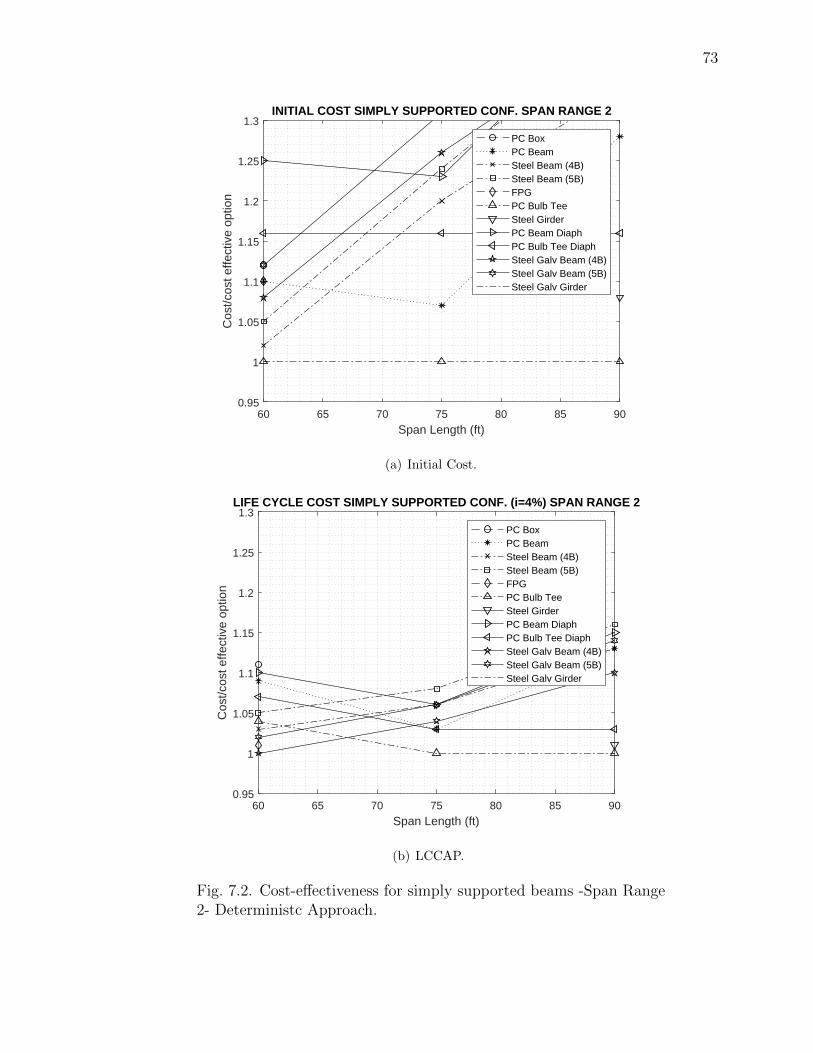
73

60 65 70 75 80 85 90

Span Length (ft)

0.95

1

1.05

1.1

1.15

1.2

1.25

1.3

Cos

t/cos

t effe

ctiv

e op

tion


PC BoxPC BeamSteel Beam (4B)Steel Beam (5B)FPGPC Bulb TeeSteel GirderPC Beam DiaphPC Bulb Tee DiaphSteel Galv Beam (4B)Steel Galv Beam (5B)Steel Galv Girder

(a) Initial Cost.

60 65 70 75 80 85 90

Span Length (ft)

0.95

1

1.05

1.1

1.15

1.2

1.25

1.3

Cos

t/cos

t effe

ctiv

e op

tion


PC BoxPC BeamSteel Beam (4B)Steel Beam (5B)FPGPC Bulb TeeSteel GirderPC Beam DiaphPC Bulb Tee DiaphSteel Galv Beam (4B)Steel Galv Beam (5B)Steel Galv Girder

(b) LCCAP.


74

90 95 100 105 110 115 120 125 130

Span Length (ft)

0.95

1

1.05

1.1

1.15

1.2

1.25

1.3

Cos

t/cos

t effe

ctiv

e op

tion


PC BeamSteel Beam (4B)Steel Beam (5B)PC Bulb TeeSteel GirderPC Beam DiaphPC Bulb Tee DiaphSteel Galv Beam (4B)Steel Galv Beam (5B)Steel Galv Girder

(a) Initial Cost.

90 95 100 105 110 115 120 125 130

Span Length (ft)

0.95

1

1.05

1.1

1.15

1.2

1.25

1.3

Cos

t/cos

t effe

ctiv

e op

tion


PC BeamSteel Beam (4B)Steel Beam (5B)PC Bulb TeeSteel GirderPC Beam DiaphPC Bulb Tee DiaphSteel Galv Beam (4B)Steel Galv Beam (5B)Steel Galv Girder

(b) LCCAP.


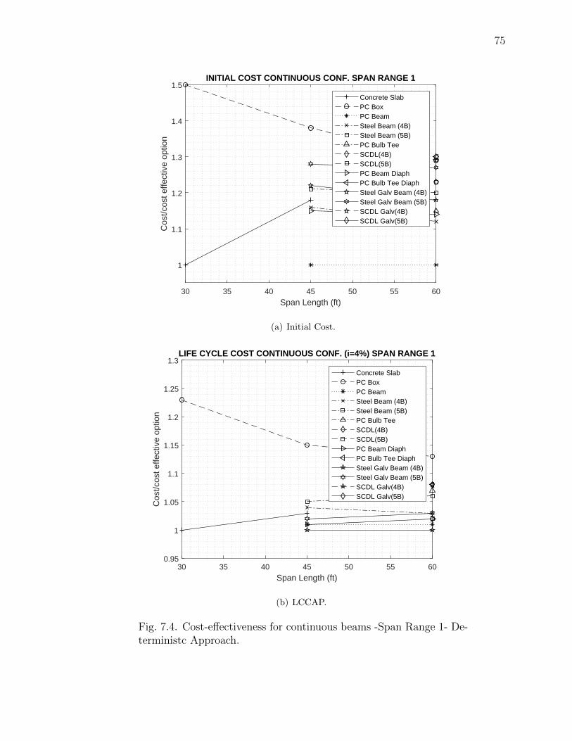
75

30 35 40 45 50 55 60

Span Length (ft)

1

1.1

1.2

1.3

1.4

1.5

Cos

t/cos

t effe

ctiv

e op

tion

INITIAL COST CONTINUOUS CONF. SPAN RANGE 1

Concrete SlabPC BoxPC BeamSteel Beam (4B)Steel Beam (5B)PC Bulb TeeSCDL(4B)SCDL(5B)PC Beam DiaphPC Bulb Tee DiaphSteel Galv Beam (4B)Steel Galv Beam (5B)SCDL Galv(4B)SCDL Galv(5B)

(a) Initial Cost.

30 35 40 45 50 55 60

Span Length (ft)

0.95

1

1.05

1.1

1.15

1.2

1.25

1.3

Cos

t/cos

t effe

ctiv

e op

tion

LIFE CYCLE COST CONTINUOUS CONF. (i=4%) SPAN RANGE 1

Concrete SlabPC BoxPC BeamSteel Beam (4B)Steel Beam (5B)PC Bulb TeeSCDL(4B)SCDL(5B)PC Beam DiaphPC Bulb Tee DiaphSteel Galv Beam (4B)Steel Galv Beam (5B)SCDL Galv(4B)SCDL Galv(5B)

(b) LCCAP.

Fig. 7.4. Cost-effectiveness for continuous beams -Span Range 1- De-terministc Approach.

76

60 65 70 75 80 85 90

Span Length (ft)

1

1.1

1.2

1.3

1.4

1.5

Cos

t/cos

t effe

ctiv

e op

tion


PC BoxPC BeamSteel Beam (4B)Steel Beam (5B)PC Bulb TeeSCDL(4B)SCDL(5B)Steel GirderPC Beam DiaphPC Bulb Tee DiaphSteel Galv Beam (4B)Steel Galv Beam (5B)Steel Galv GirderSCDL Galv(4B)SCDL Galv(5B)

(a) Initial Cost.

60 65 70 75 80 85 90

Span Length (ft)

0.95

1

1.05

1.1

1.15

1.2

1.25

1.3

Cos

t/cos

t effe

ctiv

e op

tion


PC BoxPC BeamSteel Beam (4B)Steel Beam (5B)PC Bulb TeeSCDL(4B)SCDL(5B)Steel GirderPC Beam DiaphPC Bulb Tee DiaphSteel Galv Beam (4B)Steel Galv Beam (5B)Steel Galv GirderSCDL Galv(4B)SCDL Galv(5B)

(b) LCCAP.


77

90 95 100 105 110 115 120 125 130

Span Length (ft)

1

1.1

1.2

1.3

1.4

1.5

Cos

t/cos

t effe

ctiv

e op

tion


PC Bulb TeeSteel GirderPC Bulb Tee DiaphSteel Galv Girder

(a) Initial Cost.

90 95 100 105 110 115 120 125 130

Span Length (ft)

0.95

1

1.05

1.1

1.15

1.2

1.25

1.3

Cos

t/cos

t effe

ctiv

e op

tion


PC Bulb TeeSteel GirderPC Bulb Tee DiaphSteel Galv Girder

(b) LCCAP.


78

FPG system needs a special discussion. As shown, the FPG option could be

considered as a cost-effective solution depending on the span length of the structure.

Nonetheless, a more accurate cost estimation of construction cost, not only for steel

elements but also for prefabricated composite modules, is needed to demonstrate that

viability of this system.

7.4 Life-cycle cost analysis -Stochastic analysis

The deterministic analysis could be useful as a first approximation to assess the

superstructure selection. However, and as it is seen in Figures 7.1 to 7.6 the ERLCCAP

difference between the different alternatives is minimal and therefore a decision maker

will not have a clear preference on a superstructure type. This is especially true given

the fact that only average values where used. In other words, only a single case

is examined but there is multiple other combinations that are omitted. As shown

before, there is an inherent probabilistic nature associated with all the costs involved.

Henceforth, a Monte Carlo Simulation (MCS) is used to assess this problem.

7.4.1 Monte Carlo Simulation (MCS)

As defined by Ang and Tang [66], ”simulation is the process of replicating the

real world based on a set of assumptions and conceived models of reality”. When the

problem is based on random variables with assumed or known probability distribu-

tions, the Monte Carlo simulation (MCS) method is very useful. Generally speaking,

MCS method is a repetition of different simulations, using a different set of values of

the random variable, based on the corresponding probability distribution. The deter-

ministic analysis is then considered as a single simulation process. For computational

purposes, random numbers are generated by a systematic procedure, those are known

as pseudo random. However, its periodicity as well as their randomness feature can be

assured using different algorithms, that are generally included in software packages.

79

Iterations

The number of iterations needed are highly dependant on the type of sampling

chosen for the simulation process. There are various methods, including: random

sampling, stratified sampling and latin hyperchube sampling. Random sampling is

the most intuitive and was the most used during the early development of the MCS

process. One of its drawbacks is that when few iterations are used, it is possible that

not all the input PDF is sampled. In contrast, the stratified sampling techniques (the

latin hypercube is a ramification of it) divides the PDF in strata (or hypercube) and

then a sample is obtained randomly within the random selected strata. As a conse-

quence, the PDF is better represented during the simulation with fewer iterations.

Comparison between the different sampling techniques can be consulted in the work

done by Beckman et al. [67]. Generally speaking, convergence is achieved faster using

stratified methods.

Minimum iterations needed for random sampling depends on the confidence level

desired, and is based in the central limit theorem (CLT), assuming that the final

result will be represented most likely by the normal or lognormal distribution. On

the other hand, stratified sampling convergence is achieved when additional iterations

do not change greatly the statistics of the output distribution. In this case, variation

on the output mean and output standard derivation is checked for a given example of

LCCAP. Figure 7.7 presents the coverage test to determine the number of iteration

needed for the simulation. It shows the normalized output mean and output standard

deviation of the LCCAP example depending on the number of iterations (simply

supported slab bridge, span=30-ft). As it is shown, output mean converges rapidly

(close to 1,000 iterations), while the output standard deviation converges much more

slowly, close to 10,000 iterations. The greater number of iterations needed for both

statistic outputs is then chosen.

The MCS was done using the Microsoft excel complementary software called

@RISK, developed by Palisade software company. The simulations used in this doc-

80

101 102 103 104 105 106

Iterations

0.993

0.994

0.995

0.996

0.997

0.998

0.999

1

Nor

mal

ized

out

put m

ean

0.9

0.91

0.92

0.93

0.94

0.95

0.96

0.97

0.98

0.99

1

Nor

mal

ized

out

put S

TD

MC Latin Hypercube sampling - output mean and STD convergence

Output MeanOutput STD

Fig. 7.7. Latin hypercube sampling for convergence of output meanand standard deviation of LCCAP SSB slab bridge, 30-ft

ument uses a random number generator based on Mersenne Twister pseudo random

numbers, latin hypercube sampling and 10,000 iterations per simulation.

7.4.2 Stochastic dominance (SD)

The concept of Stochastic Dominance (SD) is used to define one of the methods

used to categorize an alternative among others in a sense that “there will be one

investment which is better than (or equal to) all of the other available investments”

[68]. This categorization, when the decision makers only has partial information

available, is also known as partial ordering, which is the case of the SD.

In order to categorize the alternatives, the process divides the feasible set (FS,

i.e. a set composed by all possible alternatives), into the efficient set (ES) which

81

is composed by all the alternatives that satisfy the decision requirement, and the

inefficient set (IS) that contains the alternatives that are excluded from the decision

rule. Those two sets are mutually exclusive and comprehensive, and are shown in

Figure 7.8.

A

C

E

B

D

F

ES

IS

FS

Fig. 7.8. Feasible (FS), Efficient (ES) and Inefficient (IS) sets.

The decision rule is based on the “dominance” of one alternative over the other.

This dominance could be represented by first, second, third or nth degree of domi-

nance. Namely, the general rule of thumb is to consider the ES as the group of none

dominating alternatives, and the IS as the complementary group of the FS. This is

especially true for cases in which a higher chance of positive revenues is intended

when negative results are possible as the case of the utility functions (examples given

in [68], [69], [70], [71], [72] and [73]). However, for the case of this study, the objective

is to find the alternative with the lower price, i.e. the alternative with a higher prob-

ability to have a lower price. Henceforth, the decision rule used to divide the FS is

such that the ES will conglomerate the alternative that is dominated by all the other

alternatives and the IS the complementary options. The concept of “dominance”

82

is better understood using the different levels of stochastic dominance explained as

follows. Mathematical proof for all the stochastic dominance levels presented here

can be found in the work done by Levy [68]. Additionally, if an alternative (A) is

dominated by another (B), no matter the degree of dominance, it is considered that

A is preferred to B, A � B. However, if the result does not conclude dominance,

it is considered that there is no preference between the alternatives and the decision

maker is indifferent between the options, A ∼ B.

First stochastic dominance (FSD)

The FSD criterion is a way to establish if an alternative dominates (or not) another

alternative if the only information available is that the set of utility functions (U)

considered belongs to the set of non decreasing utility functions (U1), U ∈ U1, and

the first derivative of U is grater than or equal to 0, U ′ ≥ 0.

If F and G are the CDFs of two different alternatives, F dominates G (denoted

as FD1G where D1 means first degree of dominance) if and only if F (x) ≤ G(x) for

all values of x, and there is at least some x0 for which a strong inequality holds. Let

the difference of the two considered CDFs be I(x) such as I(x) = G(x)− F (x), then

FD1G if and only if I(x) ≥ 0 for all x and I(x) > 0 for at least one x0. Figure

7.9 shows an example of FSD for 75-ft simply supported beams. In this case, four

painted structural steel rolled beams option (F ) dominates the prestressed concrete

AASTHO beams option (G) by first degree. Then, prestressed concrete AASTHO

beams are preferred, G�1F .

Second stochastic dominance (SSD)

In the case that two alternatives do not satisfy the FSD requirements, a stronger

theorem is needed for investors most risk averse. For concave utility functions (U2),

or in other words, utility functions (U) such that U ′ ≥ 0, and U ′′ ≤ 0, there must

83

3 4 5 6 7 8

LCAAP ($) 105

0

0.1

0.2

0.3

0.4

0.5

0.6

0.7

0.8

0.9

1

Den

sity

-0.2

0

0.2

0.4

0.6

0.8

1

Nor

mal

ized

Den

sity

Diff

eren

tial

CDF Simply Supported Beams Span=75ft

F(x)=CDF Struc. Steel 4B PaintG(x)=CDF PS Conc BeamsI(x)=G(x)-F(x)

Fig. 7.9. FSD example for simply supported beams, span=75-ft.

be a utility function U such that, for two alternatives F and G,x∫a

G(t)dt ≤x∫a

F (t)dt.

Then, F dominates G by SSD (denoted as FD2G where D2 means second degree of

dominance) if and only if I(x) ≡x∫a

[G(t) − F (t)]dt ≥ 0 for all x ∈ [a, b] and there is

at least one x0 for which there is an strict inequality. Additionally, it is also stated

that if FD1G, then FD2G. This is especially important when you have multiple

alternatives to compare in order to minimize the number of comparisons.

Figure 7.10 presents an example of SSD for two simply supported beams with a

span of 45-ft. As it can be seen clearly in the Figure, alternative F (concrete slab

option) does not dominate alternative G (prestressed concrete bulb tee option) in first

degree because both CDFs crossed each other in multiple points. Additionally, it is

presented in the right y axis, the normalized area under the CDF differential, I(x). It

is proved that F dominates G in second degree, which means that a decision maker

84

will be inclined to chose the prestressed concrete bulb tee option over the concrete

slab option, G �2 F .

Nonetheless, there are cases in which the comparison between different alternatives

using FSD and SSD is not enough to clearly select an option among the others. In

those cases, the concept of almost stochastic dominance proposed by Leshno and

Levy [70] is useful. This method is intended to identify a preference of an alternative

among others for “most” decision makers but not “all” of them.

2 2.5 3 3.5 4 4.5

LCAAP ($) 105

0

0.1

0.2

0.3

0.4

0.5

0.6

0.7

0.8

0.9

1

Den

sity

0

0.1

0.2

0.3

0.4

0.5

0.6

0.7

0.8

0.9

1

Nor

mal

ized

Are

a un

der

the

CD

F D

iffer

entia

l


F(x)=CDF Conccrete SlabG(x)=CDF PS Conc BeamI(x)=int(G(x))-int(F(x))

Fig. 7.10. SSD example for simply supported beams, span=45-ft.

Almost first stochastic dominance (AFSD)

AFDS rules are based on the definition of FDS. However, while FSD stated that

for two alternatives with different CDFs denoted as F and G, the following inequity,

F (x) ≤ G(x), must be true for all x and strictly true for at least one x0. The AFSD,

85

however, requires that the previous inequality must be true for “most” of the range

S, allowing a small “violation” of the dominance. The violation range of the FSD

(S1) is denoted as

S1(F,G) = {x : G(x) < F (x)} (7.4)

then, the ratio between the violation area of the FSD and the total area between the

CDF’s (ε1) is

ε1 ≡

∫S1

(F (x)−G(x))dx∫S

| F (x)−G(x) | dx(7.5)

Leshno and Levy [70] stated that almost stochastic dominance holds when ε1 is

lesser than 50%, 0 < ε1 < 0.5. The limiting value for ε is strictly related with the

level of risk aversion, it means than the smaller the value, the higher the risk aversion

and the stronger the dominance. This inequality is also related with the normal SD,

when it holds, then the standard FSD or SSD holds.

Figure 7.11 illustrates the AFSD approach for simply supported beams with spans

of 75-ft. Alternative F , prestressed concrete AASHTO beams, and alternative G, pre-

stressed concrete bulb tee with intermediate diaphragms, are tested for dominance.

The FSD violation area between the two CDF’s is shaded in the Figure. The vi-

olation ratio, ε1, is equal to 0.11 which is less than 0.50. Therefore, prestressed

concrete AASHTO beams dominates prestressed concrete bulb tee with intermediate

diaphragms option, G�almost1F .

Almost second stochastic dominance (ASSD)

On the other hand, there are cases in which AFSD is not enough to select an

option among others. For these cases, ASSD rules could be used. Consider again two

different CDFs alternatives F and G, then, F almost dominates G in second degree

86

Fig. 7.11. AFSD example for simply supported beams, span=75-ft.

ifx∫a

G(t)dt ≤x∫a

F (t)dt for most of the range S, but not for all of it. The violation

range of the SSD (S2) is defined by

S2(F,G) =

{x : G(x) < F (x);

x∫a

G(t)dt ≤x∫a

F (t)dt

}(7.6)

then, the ration between the violation area of the SSD and the total area between

the CDFs (ε2) is, where S2 is the complement area of S2, i.e S2 ∩ S2 = S

ε2 ≡

∫S2

(F (x)−G(x))dx∫S2

(G(x)− F (x))dx+∫S2

(F (x)−G(x))dx(7.7)

87

As stated in AFSD, for ASSD, F almost dominate G in the second degree if

0 < ε2 < 0.5. However, for simplicity, Levy [69] proposed the Equation 7.7 for an

easy programmable algorithm as follows:

ε2 =

∫S2

(F (x)−G(x))dx

E[F ] + E[G] + 2∫S2

(F (x)−G(x))dx(7.8)

Figure 7.12 illustrates the ASSD approach for simply supported beams with spans

of 90-ft. Alternative F , galvanized structural steel girders, and alternative G, pre-

stressed concrete bulb tee, are tested for dominance. The SSD violation area between

the two CDFs is shaded in the Figure. The violation ratio, ε2, is equal to 0.21 which

is less than 0.50. Therefore, the prestressed concrete bulb tee alternative dominates

the galvanized structural steel girders option, F�almost2G.

Fig. 7.12. ASSD example for simply supported beams, span=90-ft.

88

7.4.3 Superstructure selection

Mirroring the process made in the deterministic approach, the first step in order to

select the most cost effective superstructure is to find the most cost effective life-cycle

cost profile (LCCP) for each superstructure type. Since all LCCP for each type have

the same SL, it is indifferent if the LCCA or the LCCAP is used to do the analysis.

In this case, the LCCA is the base of the LCCP selection using SD. Additionally,

there is no necessity to evaluate the cost effectiveness of all LCCP using all available

spans since all factors only will vary on proportion but not in differences. Finally,

and base on the LCCP presented in Appendix C, as a general approach, LCCPs can

be grouped in main categories: concrete structures, prestressed concrete structures,

prestressed concrete structures with diaphragms, structural steel painted structures

and structural steel galvanized structures. Therefore, only one case is presented for

each of the main groups. The results presented herein corresponds to 30-ft long

bridges with simply supported beams and 60-ft long for continuous beams (SDCL

and prestressed concrete options with diaphragms).

Table 7.2 summarizes the different alternatives considered for each group. Those

alternatives are the combination of working actions such as: washing and cleaning of

the deck surface (WC), sealing of the concrete deck surface (SC), full depth concrete

patching (CP), concrete overlays (O), superstructure removal (BD), concrete slab

reconstruction (DR), bearing replacements (BR), steel elements full painting (FP),

steel elements spot painting (SP), and structural steel recycle (SR). As a general rule

of thumb, the table presents the current INDOT working action procedure (called

INDOT in the table), and different alternatives depending on the superstructure

type and the working actions considered (in the table, alternatives A to E).

Figures 7.13 and 7.14 present the CDFs for the concrete and structural steel

groups respectively. The SD analysis shows that for concrete structures Alt A � Alt

B �2 INDOT, for prestressed concrete structures Alt A �almost1 Alt B �2 INDOT,

for prestressed concrete structures with diaphragms Alt A �almost1 Alt B � INDOT,

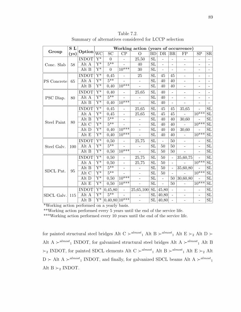
89

Table 7.2.Summary of alternatives considered for LCCP selection

GroupS L

OptionWorking action (years of occurrence)

(ys) WC SC CP O BD DR BR FP SP SR

Conc. Slab 58

INDOT Y* 0 - 25,50 SL - - - - -Alt A Y* 5** - 40 SL - - - - -Alt B Y* 0 10*** 30 SL - - - - -

PS Concrete 65

INDOT Y* 0,45 - 25 SL 45 45 - - -Alt A Y* 5** - - SL 40 40 - - -Alt B Y* 0,40 10*** - SL 40 40 - - -

PSC Diap. 80

INDOT Y* 0,40 - 25,65 SL 40 - - - -Alt A Y* 5** - - SL 40 - - - -Alt B Y* 0,40 10*** - SL 40 - - - -

Steel Paint 80

INDOT Y* 0,45 - 25,65 SL 45 45 35,65 - SLAlt A Y* 0,45 - 25,65 SL 45 45 - 10*** SLAlt B Y* 5** - - SL 40 40 30,60 - SLAlt C Y* 5** - - SL 40 40 - 10*** SLAlt D Y* 0,40 10*** - SL 40 40 30,60 - SLAlt E Y* 0,40 10*** - SL 40 40 - 10*** SL

Steel Galv. 100

INDOT Y* 0,50 - 25,75 SL - 50 - - SLAlt A Y* 5** - - SL 50 50 - - SLAlt B Y* 0,50 10*** - SL 50 50 - - SL

SDCL Pnt. 95

INDOT Y* 0,50 - 25,75 SL 50 - 35,60,75 - SLAlt A Y* 0,50 - 25,75 SL 50 - - 10*** SLAlt B Y* 5** - - SL 50 - 35,60,80 - SLAlt C Y* 5** - - SL 50 - - 10*** SLAlt D Y* 0,50 10*** - SL - 50 30,60,80 - SLAlt E Y* 0,50 10*** - SL - 50 - 10*** SL

SDCL Galv. 115

INDOT Y* 0,45,80 - 25,65,100 SL 45,80 - - - SLAlt A Y* 5** - - SL 40,80 - - - SLAlt B Y* 0,40,80 10*** - SL 40,80 - - - SL

*Working action performed on a yearly basis.**Working action performed every 5 years until the end of the service life.***Working action performed every 10 years until the end of the service life.

for painted structural steel bridges Alt C �almost1 Alt B �almost1 Alt E �2 Alt D �

Alt A �almost1 INDOT, for galvanized structural steel bridges Alt A �almost1 Alt B

�2 INDOT, for painted SDCL elements Alt C �almost1 Alt B �almost1 Alt E �2 Alt

D � Alt A �almost1 INDOT, and finally, for galvanized SDCL beams Alt A �almost1Alt B �2 INDOT.

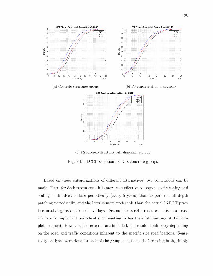
90

(a) Concrete structures group (b) PS concrete structures group

(c) PS concrete structures with diaphragms group

Fig. 7.13. LCCP selection - CDFs concrete groups

Based on these categorizations of different alternatives, two conclusions can be

made. First, for deck treatments, it is more cost effective to sequence of cleaning and

sealing of the deck surface periodically (every 5 years) than to perform full depth

patching periodically, and the later is more preferable than the actual INDOT prac-

tice involving installation of overlays. Second, for steel structures, it is more cost

effective to implement periodical spot painting rather than full painting of the com-

plete element. However, if user costs are included, the results could vary depending

on the road and traffic conditions inherent to the specific site specifications. Sensi-

tivity analyses were done for each of the groups mentioned before using both, simply

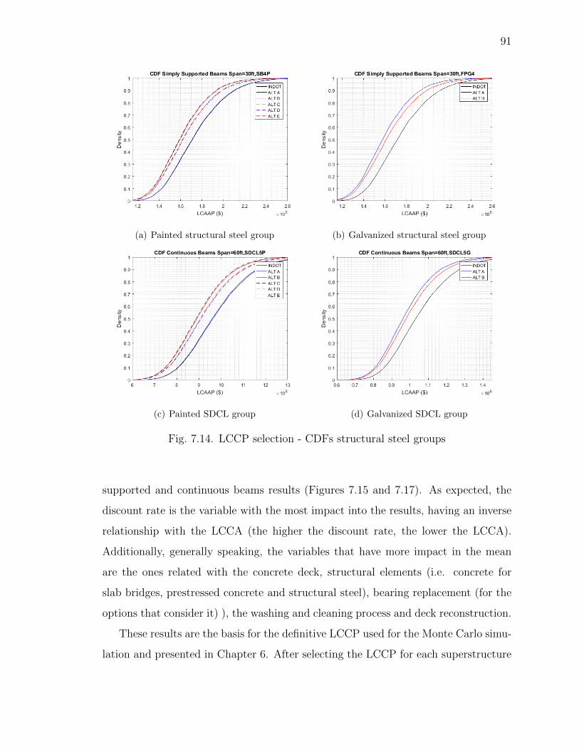
91

(a) Painted structural steel group (b) Galvanized structural steel group

(c) Painted SDCL group (d) Galvanized SDCL group

Fig. 7.14. LCCP selection - CDFs structural steel groups

supported and continuous beams results (Figures 7.15 and 7.17). As expected, the

discount rate is the variable with the most impact into the results, having an inverse

relationship with the LCCA (the higher the discount rate, the lower the LCCA).

Additionally, generally speaking, the variables that have more impact in the mean

are the ones related with the concrete deck, structural elements (i.e. concrete for

slab bridges, prestressed concrete and structural steel), bearing replacement (for the

options that consider it) ), the washing and cleaning process and deck reconstruction.

These results are the basis for the definitive LCCP used for the Monte Carlo simu-

lation and presented in Chapter 6. After selecting the LCCP for each superstructure

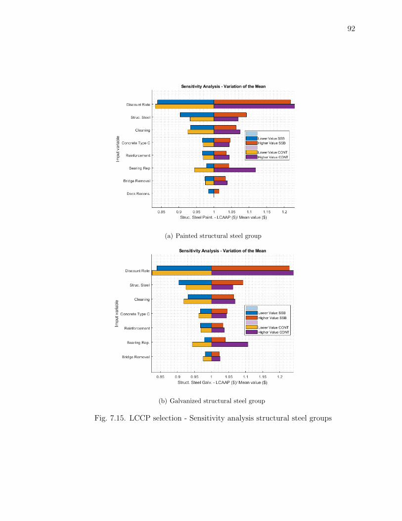
92

(a) Painted structural steel group

(b) Galvanized structural steel group

Fig. 7.15. LCCP selection - Sensitivity analysis structural steel groups

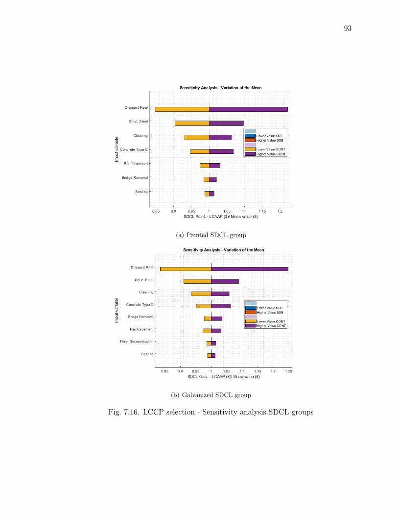
93

(a) Painted SDCL group

(b) Galvanized SDCL group

Fig. 7.16. LCCP selection - Sensitivity analysis SDCL groups

94

(a) Concrete structures group

(b) PS concrete structures group

(c) PS concrete structures with diaphragms group

Fig. 7.17. LCCP selection - Sensitivity analysis concrete groups

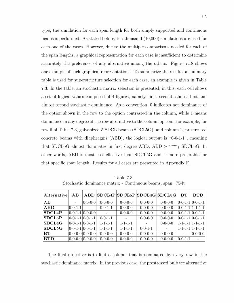
95

type, the simulation for each span length for both simply supported and continuous

beams is performed. As stated before, ten thousand (10,000) simulations are used for

each one of the cases. However, due to the multiple comparisons needed for each of

the span lengths, a graphical representation for each case is insufficient to determine

accurately the preference of any alternative among the others. Figure 7.18 shows

one example of such graphical representations. To summarize the results, a summary

table is used for superstructure selection for each case, an example is given in Table

7.3. In the table, an stochastic matrix selection is presented, in this, each cell shows

a set of logical values composed of 4 figures, namely, first, second, almost first and

almost second stochastic dominance. As a convention, 0 indicates not dominance of

the option shown in the row to the option contrasted in the column, while 1 means

dominance in any degree of the row alternative to the column option. For example, for

row 6 of Table 7.3, galvanized 5 SDCL beams (SDCL5G), and column 2, prestressed

concrete beams with diaphragms (ABD), the logical output is “0-0-1-1”, meaning

that SDCL5G almost dominates in first degree ABD, ABD �almost1 SDCL5G. In

other words, ABD is most cost-effective than SDCL5G and is more preferable for

that specific span length. Results for all cases are presented in Appendix F.

Table 7.3.Stochastic dominance matrix - Continuous beams, span=75-ft

Alternative AB ABD SDCL4P SDCL5P SDCL4G SDCL5G BT BTD

AB - 0-0-0-0 0-0-0-0 0-0-0-0 0-0-0-0 0-0-0-0 0-0-1-1 0-0-1-1ABD 0-0-1-1 - 0-0-1-1 0-0-0-0 0-0-0-0 0-0-0-0 0-0-1-1 1-1-1-1SDCL4P 0-0-1-1 0-0-0-0 - 0-0-0-0 0-0-0-0 0-0-0-0 0-0-1-1 0-0-1-1SDCL5P 0-0-1-1 0-0-1-1 0-0-1-1 - 0-0-0-0 0-0-0-0 0-0-1-1 0-0-1-1SDCL4G 0-0-1-1 0-0-1-1 1-1-1-1 1-1-1-1 - 0-0-0-0 1-1-1-1 1-1-1-1SDCL5G 0-0-1-1 0-0-1-1 1-1-1-1 1-1-1-1 0-0-1-1 - 1-1-1-1 1-1-1-1BT 0-0-0-0 0-0-0-0 0-0-0-0 0-0-0-0 0-0-0-0 0-0-0-0 - 0-0-0-0BTD 0-0-0-0 0-0-0-0 0-0-0-0 0-0-0-0 0-0-0-0 0-0-0-0 0-0-1-1 -

The final objective is to find a column that is dominated by every row in the

stochastic dominance matrix. In the previous case, the prestressed bulb tee alternative

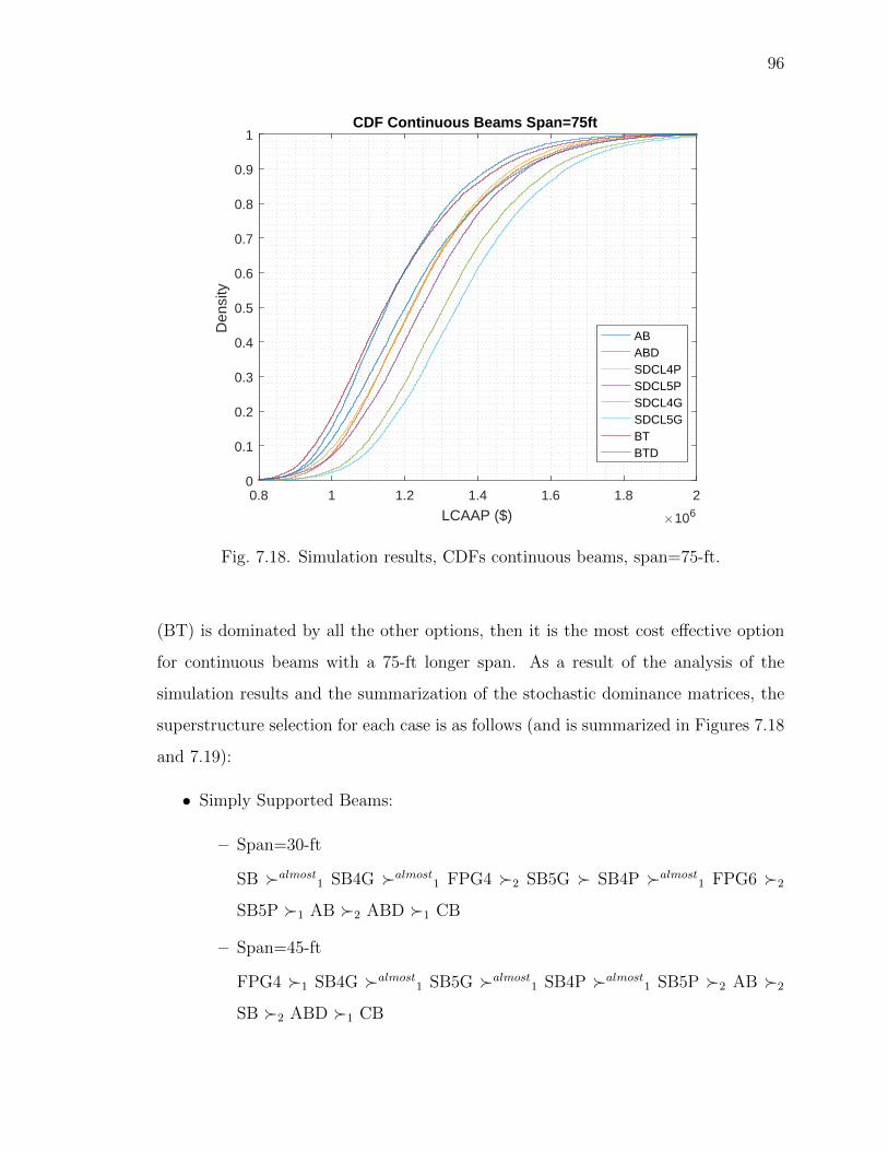
96

0.8 1 1.2 1.4 1.6 1.8 2

LCAAP ($) 106

0

0.1

0.2

0.3

0.4

0.5

0.6

0.7

0.8

0.9

1

Den

sity

CDF Continuous Beams Span=75ft

ABABDSDCL4PSDCL5PSDCL4GSDCL5GBTBTD

Fig. 7.18. Simulation results, CDFs continuous beams, span=75-ft.

(BT) is dominated by all the other options, then it is the most cost effective option

for continuous beams with a 75-ft longer span. As a result of the analysis of the

simulation results and the summarization of the stochastic dominance matrices, the

superstructure selection for each case is as follows (and is summarized in Figures 7.18

and 7.19):

• Simply Supported Beams:

– Span=30-ft

SB �almost1 SB4G �almost1 FPG4 �2 SB5G � SB4P �almost1 FPG6 �2

SB5P �1 AB �2 ABD �1 CB

– Span=45-ft

FPG4 �1 SB4G �almost1 SB5G �almost1 SB4P �almost1 SB5P �2 AB �2

SB �2 ABD �1 CB

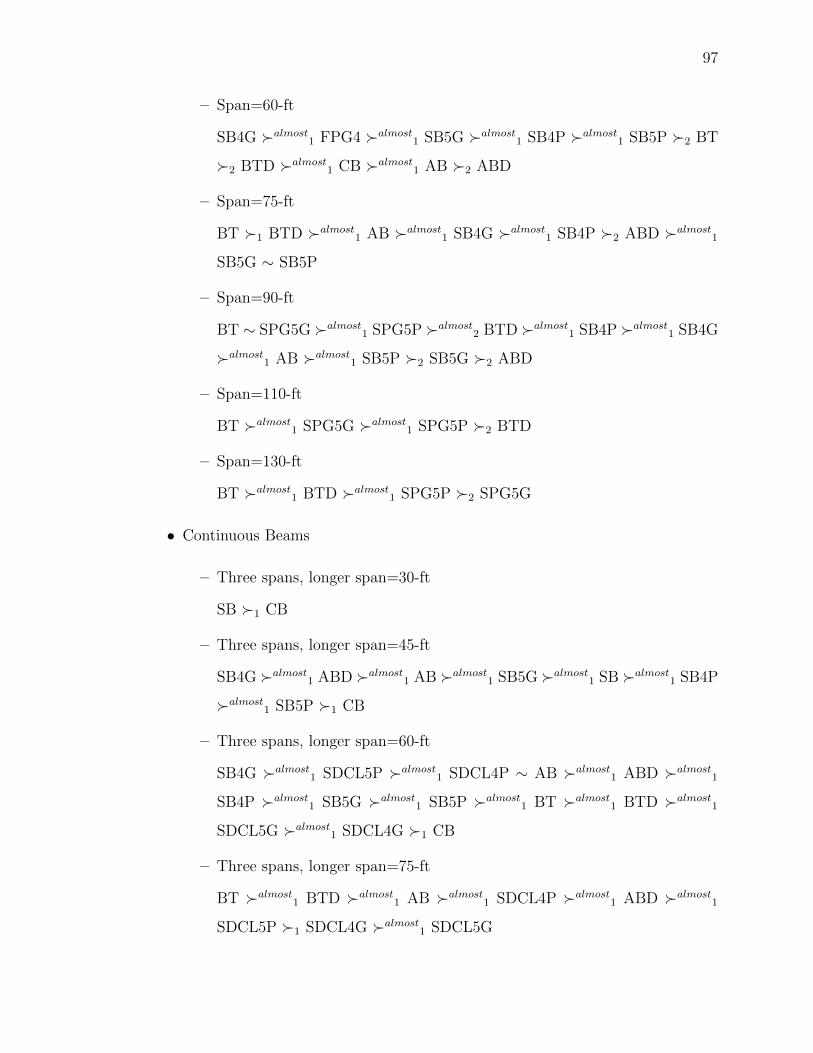
97

– Span=60-ft

SB4G �almost1 FPG4 �almost1 SB5G �almost1 SB4P �almost1 SB5P �2 BT

�2 BTD �almost1 CB �almost1 AB �2 ABD

– Span=75-ft

BT �1 BTD �almost1 AB �almost1 SB4G �almost1 SB4P �2 ABD �almost1SB5G ∼ SB5P

– Span=90-ft

BT ∼ SPG5G �almost1 SPG5P �almost2 BTD �almost1 SB4P �almost1 SB4G

�almost1 AB �almost1 SB5P �2 SB5G �2 ABD

– Span=110-ft

BT �almost1 SPG5G �almost1 SPG5P �2 BTD

– Span=130-ft

BT �almost1 BTD �almost1 SPG5P �2 SPG5G

• Continuous Beams

– Three spans, longer span=30-ft

SB �1 CB


SB4G �almost1 ABD �almost1 AB �almost1 SB5G �almost1 SB �almost1 SB4P

�almost1 SB5P �1 CB


SB4G �almost1 SDCL5P �almost1 SDCL4P ∼ AB �almost1 ABD �almost1SB4P �almost1 SB5G �almost1 SB5P �almost1 BT �almost1 BTD �almost1SDCL5G �almost1 SDCL4G �1 CB


BT �almost1 BTD �almost1 AB �almost1 SDCL4P �almost1 ABD �almost1SDCL5P �1 SDCL4G �almost1 SDCL5G

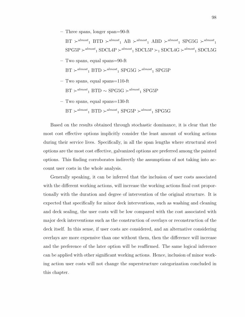
98


BT �almost1 BTD �almost1 AB �almost1 ABD �almost1 SPG5G �almost1SPG5P�almost1 SDCL4P�almost1 SDCL5P�1 SDCL4G�almost1 SDCL5G

– Two spans, equal spans=90-ft

BT �almost1 BTD �almost1 SPG5G �almost1 SPG5P


BT �almost1 BTD ∼ SPG5G �almost1 SPG5P


BT �almost1 BTD �almost1 SPG5P �almost1 SPG5G

Based on the results obtained through stochastic dominance, it is clear that the

most cost effective options implicitly consider the least amount of working actions

during their service lives. Specifically, in all the span lengths where structural steel

options are the most cost effective, galvanized options are preferred among the painted

options. This finding corroborates indirectly the assumptions of not taking into ac-

count user costs in the whole analysis.

Generally speaking, it can be inferred that the inclusion of user costs associated

with the different working actions, will increase the working actions final cost propor-

tionally with the duration and degree of intervention of the original structure. It is

expected that specifically for minor deck interventions, such as washing and cleaning

and deck sealing, the user costs will be low compared with the cost associated with

major deck interventions such as the construction of overlays or reconstruction of the

deck itself. In this sense, if user costs are considered, and an alternative considering

overlays are more expensive than one without them, then the difference will increase

and the preference of the later option will be reaffirmed. The same logical inference

can be applied with other significant working actions. Hence, inclusion of minor work-

ing action user costs will not change the superstructure categorization concluded in

this chapter.

99

Fig. 7.19. Superstructure selection chart - Simply supported beams

100

Fig. 7.20. Superstructure selection chart - Continuous beams

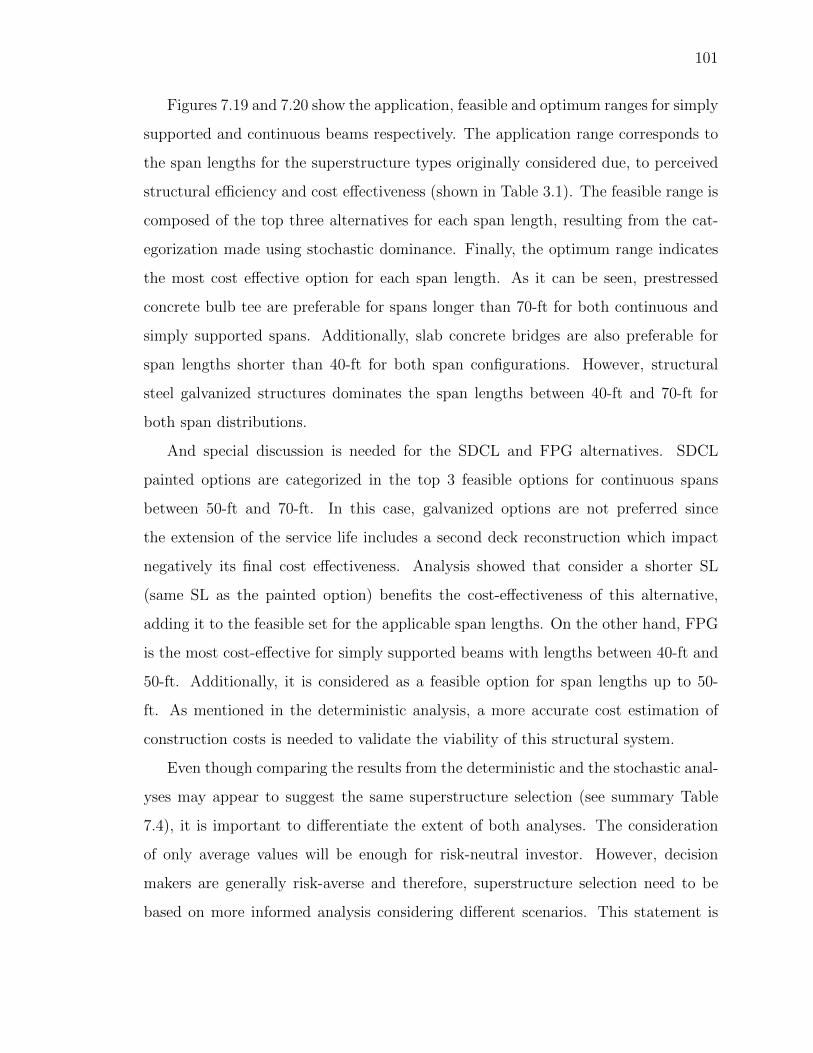
101

Figures 7.19 and 7.20 show the application, feasible and optimum ranges for simply

supported and continuous beams respectively. The application range corresponds to

the span lengths for the superstructure types originally considered due, to perceived

structural efficiency and cost effectiveness (shown in Table 3.1). The feasible range is

composed of the top three alternatives for each span length, resulting from the cat-

egorization made using stochastic dominance. Finally, the optimum range indicates

the most cost effective option for each span length. As it can be seen, prestressed

concrete bulb tee are preferable for spans longer than 70-ft for both continuous and

simply supported spans. Additionally, slab concrete bridges are also preferable for

span lengths shorter than 40-ft for both span configurations. However, structural

steel galvanized structures dominates the span lengths between 40-ft and 70-ft for

both span distributions.

And special discussion is needed for the SDCL and FPG alternatives. SDCL

painted options are categorized in the top 3 feasible options for continuous spans

between 50-ft and 70-ft. In this case, galvanized options are not preferred since

the extension of the service life includes a second deck reconstruction which impact

negatively its final cost effectiveness. Analysis showed that consider a shorter SL

(same SL as the painted option) benefits the cost-effectiveness of this alternative,

adding it to the feasible set for the applicable span lengths. On the other hand, FPG

is the most cost-effective for simply supported beams with lengths between 40-ft and

50-ft. Additionally, it is considered as a feasible option for span lengths up to 50-

ft. As mentioned in the deterministic analysis, a more accurate cost estimation of

construction costs is needed to validate the viability of this structural system.

Even though comparing the results from the deterministic and the stochastic anal-

yses may appear to suggest the same superstructure selection (see summary Table

7.4), it is important to differentiate the extent of both analyses. The consideration

of only average values will be enough for risk-neutral investor. However, decision

makers are generally risk-averse and therefore, superstructure selection need to be

based on more informed analysis considering different scenarios. This statement is

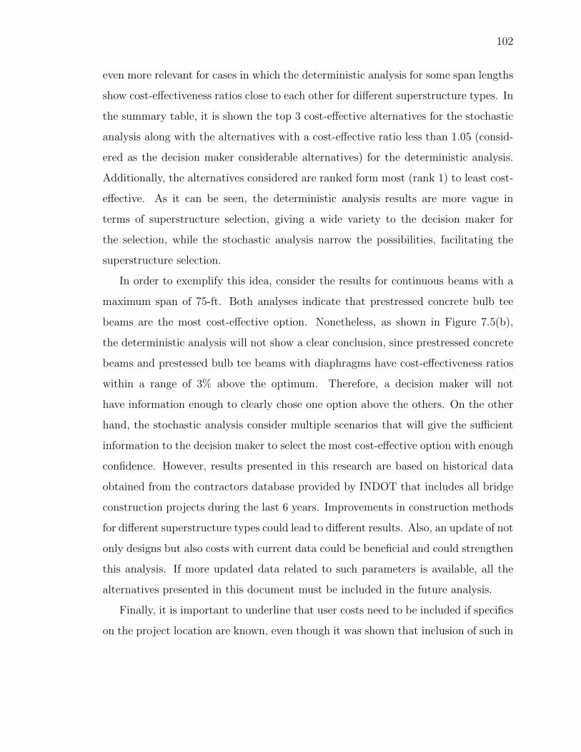
102

even more relevant for cases in which the deterministic analysis for some span lengths

show cost-effectiveness ratios close to each other for different superstructure types. In

the summary table, it is shown the top 3 cost-effective alternatives for the stochastic

analysis along with the alternatives with a cost-effective ratio less than 1.05 (consid-

ered as the decision maker considerable alternatives) for the deterministic analysis.

Additionally, the alternatives considered are ranked form most (rank 1) to least cost-

effective. As it can be seen, the deterministic analysis results are more vague in

terms of superstructure selection, giving a wide variety to the decision maker for

the selection, while the stochastic analysis narrow the possibilities, facilitating the

superstructure selection.

In order to exemplify this idea, consider the results for continuous beams with a

maximum span of 75-ft. Both analyses indicate that prestressed concrete bulb tee

beams are the most cost-effective option. Nonetheless, as shown in Figure 7.5(b),

the deterministic analysis will not show a clear conclusion, since prestressed concrete

beams and prestessed bulb tee beams with diaphragms have cost-effectiveness ratios

within a range of 3% above the optimum. Therefore, a decision maker will not

have information enough to clearly chose one option above the others. On the other

hand, the stochastic analysis consider multiple scenarios that will give the sufficient

information to the decision maker to select the most cost-effective option with enough

confidence. However, results presented in this research are based on historical data

obtained from the contractors database provided by INDOT that includes all bridge

construction projects during the last 6 years. Improvements in construction methods

for different superstructure types could lead to different results. Also, an update of not

only designs but also costs with current data could be beneficial and could strengthen

this analysis. If more updated data related to such parameters is available, all the

alternatives presented in this document must be included in the future analysis.

Finally, it is important to underline that user costs need to be included if specifics

on the project location are known, even though it was shown that inclusion of such in

103

Table 7.4.Results summary - Deterministic and stochastic analysis comparison

Span Length(ft)1

Deterministic Analysis Stochastic AnalysisSSB CONT SSB CONT

30

1. SB 1. SB 1. SB 1. SB2. SB4G - 2. SB4G 2. CB3. FGP4 - 3. FGP4 -

45

1. FPG4 1. SB4G 1. FPG4 1. SB4G2. SB4G 2. AB 2. SB4G 2. ABD3. SB5G 3. ABD 3. SB5G 3. AB

- 4. SB5G - -- 5. SB - -- 6. SB4P - -- 7. SB5P - -

60

1. SB4G 1. SB4G 1. SB4G 1. SB4G2. FPG4 2. AB 2. FPG4 2. SDCL5P3. SB5G 3. SDCL5P 3. SB5G 3*. SDCL4P4. SB4P 4. SDCL5P - 3*. AB5. BT 5. ABD - -6. SB5P 6. SB4P - -

- 7. SB5G - -

75

1. BT 1. BT 1. BT 1. BT2. AB 2. BTD 2. BTD 2. BTD3. BTD 3. AB 3. AB 3. AB4. SB4G 4. SDCL4P - -

- 5. ABD - -

90

1. BT 1. AB 1*. BT 1. BT2. SPG5G 2. BT 1*. SPG5P 2. BTD3. SPG5P 3. BTD 2. SPG5P 3. AB4. BTD 4. ABD - -

- 5. SPG5G - -- 6. SPG5P - -

90-90

- 1. BT - 1. BT- 2. BTD - 2. BTD- - - 3. SPG5G

110

1. BT 1. BT 1. BT 1. BT2. SPG5G 2. BTD 2. SPG5G 2*. BTD3. SPG5P 3. SPG5G 3. SPG5P 2*. SPG5G4. BTD 4. SPG5P - -

130

1. BT 1. BT 1. BT 1. BT2. BTD 2. BTD 2. BTD 2. BTD

- - 3. SPG5P 3. SPG5P1 Maximum span length for continuous beams (CONT)* No stochastic dominance between the two options

104

the working actions costs will not change the outcome of this study, they could have

an important impact for computation of construction and removal costs.

105

8. SUMMARY AND CONCLUSIONS

8.1 Summary

A literature review was presented on innovative cost effective solutions for short to

medium span bridges, deterioration curves and current approaches taken to conduct

a Bridge Life Cycle Cost Assessment. Additionally, information obtained from the

National Bridge Inventory (NBI) was used to summarize the most common structures

within the state and generate a design plan for the structures to analyze. Designs

covered the most common structures found in Indiana along with the innovative bridge

systems presented in this document. Bridge types used are: slab bridges (constant

thickness), prestressed concrete box beams, concrete AASHTO beams, concrete bulb

tees, structural steel folded plate beams, rolled steel beams, steel plate girders, and

finally, structural steel SDCL beams.

Three different span ranges were selected for further study. Range 1 includes

bridges with spans between 30-ft and 60-ft. Range 2 included spans between 60-ft and

90-ft. Finally, Range 3 included span lengths between 90-ft to 130-ft. Design types

were considered depending on their cost-effectiveness potential for each of the span

ranges. Spread sheets that include applicable sections of the LRFD and the Indiana

Design Manual specifications were created for every design option. The spread sheets

were then used to develop designs for a “typical” bridge selection in the appropriate

span ranges

Extensive cost allocations for agency costs were presented, including not only

initial costs involved but also long-term costs depending on the material and super-

structure type considered. No contingencies other than regular deterioration of the

bridge were considered. However, it should be mentioned that maintenance or re-

habilitation activities may affect user costs. Nonetheless, and in order to compute

106

those costs, a thorough understanding of the traffic (quantities and type of vehicles),

detour lengths, travel times and travel velocities is needed. As specified in this doc-

ument, all bridge designs have no specific location along any specific road. In other

words, traffic, velocity and detour assumptions are not made. Additionally, such

assumptions are considered an oversimplification of the problem and could impact

negatively the outcome of the LCCA comparison. Additionally, historical data were

used to determine the probability distribution that better fit the data for each pay

item considered. This information is crucial for the accurate stochastic analysis made

for each superstructure type. A method of classification is presented based on the

Kolmogorov-Smirnoff test and the Anderson-Darling test. For pay items without his-

torical data available, a PERT distribution was specified with lower and maximum

probable values equal to, respectively, 75% and 125% of the expected value. Finally,

full parameterized probability distributions for each pay item are presented.

Deterioration curves for the Indiana state highway system from work conducted

by Moomen et al. [17], Sinha et al. [20] and Cha et al. [38] were used to obtain the ser-

vice lives for each alternative. Additionally, and considering the working actions along

with the service life for each alternative, different LCCPs were proposed and the most

cost-effective were used for the LCCA comparison for each superstructure type ana-

lyzed. In addition to the regular superstructure options described before, prestressed

beam alternatives including integral abutments and intermediate diaphragms, as well

as galvanized structural steel beams were considered, including the equivalent ex-

tension of the service life of each option. In order to compare all the alternatives

considered, a life cycle present worth in perpetuity method is used. Two different

approaches were utilized for the analysis, a deterministic and a stochastic method.

For the deterministic analysis, initial cost and LCCA comparison for all span

ranges of simply supported beams and continuous beams are presented. It was

shown that the inclusion of long term-costs using LCCA generally reduces the cost-

effectiveness difference between all the alternatives for the same span length. This

reduction could be an important factor if specific site conditions are considered dur-

107

ing the analysis. If specific site conditions are known, multiple options for each span

length must be considered before choosing the best alternative.

As mentioned before, deterministic analysis reduced the cost-effectiveness differ-

ence between all the alternatives. Under those circumstances, and considering only

average values, only risk-neutral investors would take decision or whether use and

alternative or not. Nonetheless, decision makers in general are risk-averse, which re-

quires consideration of multiple scenarios in order to make a superstructure selection.

Thereupon, the stochastic analysis is used to take more informed based superstructure

selections.

A Monte Carlo simulation was used to consider multiple scenarios. Specifics on the

method and assumptions made are presented. A latin hypercube sampling system

is selected and ten thousand (10,000) simulations are considered for the analysis.

Cumulative density functions are then obtained for every scenario used. The results

of the simulation are then analyzed using the stochastic dominance principles. First,

second, almost first and almost second stochastic dominance rules are explained and

used for the categorization of the different superstructure types for each span length.

As a result, the optimal superstructure option selected is the one that is dominated

by all the other alternatives, composing in that way the efficient set and relegating

the other options to the inefficient set.

Finally, charts showing the application, feasible and optimum ranges for simply

supported and continuous beams are presented. The application range corresponds

to the span lengths which the superstructure type is originally considered and struc-

tural efficient and cost effective possible (shown in Table 3.1). The feasible range

is composed by the top three alternatives for each span length, resulted from the

stochastic dominance analysis. Finally, the optimum range indicates the most cost

effective option for each span length.

As a recommendation to practitioners, it is important to underline that user costs

need to be included if specifics on the project location are known, even though it was

shown that inclusion of such in the working actions costs will not change the outcome

108

of this study, they could have an important impact for computation of construction

and removal costs that need to be addressed.

8.2 Conclusions

Based upon the analysis conducted herein the following conclusions can be stated:

• The deterministic analysis, explicitly for simply supported beams, showed that

for Span Range 1 the slab bridge is the most cost-effective solution either consid-

ering or not considering long-term costs for spans less than 45-ft. However, for

spans longer than 35-ft, the inclusion of galvanized steel structures - specifically

the four (4) beam configuration - provided the most cost-effective alternative.

For Span Range 2, four (4) galvanized rolled steel beams are still cost-effective

for spans shorter than 65-ft, while the prestressed concrete bulb tees became

the optimal solution for longer spans. Additionally, Span Range 3 results show

that including long-term costs suggests multiple cost-effective design solutions

for spans up to 105-ft, with prestressed concrete bulb tees and galvanized steel

plate girders being the two optimal solution. Beyond this point, bulb tees are

the most cost effective solution.

• For continuous beams again for the deterministic analysis, it is shown for Span

Range 1 that slab bridges and galvanized steel continuous beams are again the

most cost effective solutions for the lower and upper parts of the span range,

respectively. However, prestressed concrete AASHTO beams are also a compet-

itive option for spans between 45 and 60-ft. In contrast, Span Range 2 suggests

that the cost-effectiveness of the SDCL system for spans up to 90-ft is not

considered as the optimum, however, it is among the most cost-effective alter-

natives. Additionally, it is noticeable that prestressed bulb tees and AASHTO

beams become more attractive for longer spans. Finally, for Span Range 3, no

variance in the cost-effectiveness of the bulb tee option is noticed between the

initial cost comparison and the inclusion of long-term costs.

109

• The stochastic analysis showed that the most cost effective options implicitly

consider the least amount of working actions during their service lives. Specif-

ically, in all the span lengths where structural steel options are the most cost

effective, galvanized options are preferred among the painted options. This find-

ing corroborates indirectly the assumptions of not taking user costs into account

in the analysis. it can be inferred that the inclusion of user costs associated with

the different working actions, will increase the working actions final cost propor-

tionally with the duration and degree of intervention of the original structure.

Thus, if user costs are considered, and an alternative considering more intrusive

actions is most costlier than one without them, then, the difference will increase

and the preference of the later option will be reaffirmed. Consequently, inclusion

of working action user costs will not change the superstructure categorization

made.

• Stochastic analysis also showed that prestressed concrete bulb tee are preferable

for spans longer than 70-ft for both continuous and simply supported spans.

Additionally, slab concrete bridges are also preferable for span lengths shorter

than 40-ft for both span configurations. However, structural steel galvanized

structures dominates the span lengths between 40-ft and 70-ft for both span

distributions. These charts and the information provided could help designers

to chose the most cost effective alternative for a given span length based on

LCCA instead of the initial cost approach, which is the base of the current

procedure.

• Strictly speaking, results obtained form both analyses suggest the same super-

structure selection (see summary Table 7.4) for every span length, however, it is

important to remark that the consideration of only average values will be enough

for risk-neutral investor. However, decision makers are generally risk-averse and

therefore, superstructure selection need to be based on more informed analysis

considering different scenarios, which are included in the stochastic analysis.

110

• Finally, the deterministic analysis results are more vague in terms of super-

structure selection, giving a wide variety to the decision maker for the final

selection, while the stochastic analysis narrow the possibilities, facilitating the

superstructure choosing.

8.3 Future Work

Even though the superstructure selection presented in this document can be con-

sidered as an starting point to more informed base superstructure selection process, it

also true that many others consideration and scenarios are needed to enrich the find-

ings of this research. Some ideas fr future work based in this research are summarized

herein:

i This study was based on bridge structures included in the National Highway

System (NHS), locally owned or minor road structures could be used to expand

this study. Inclusion of such structures may change not only the “typical”

structures considered and span configurations but also the deterioration curves

due to change in traffic conditions. As a consequence, working actions for such

structures may vary as well as their periodicity, factors that could impact greatly

the outcome of the BLCCA method.

ii Even though user costs consideration may not change the superstructure se-

lection, their consideration could be beneficial to strengthen the conclusions

of this research. To do so, a geographical division could be implemented (i.e.

northern, central and southern Indiana regions) to simplify the assumptions on

traffic. detours and truck composition upon many other factors.

iii This research was focused on Indiana infrastructure database, equivalent anal-

ysis could be made for other states, with the likelihood of obtaining different

results. However, specifically for the pay item probability function selection,

it could be possible that trends on specific PDFs depending on certain work-

111

ing actions could be analyzed as a regional behavior for colliding states. This

could be beneficial for future studies, facilitating the assumptions made by the

researcher.

iv The prediction of the service lives used in this document is based on histor-

ical data obtained from the NBI database. However, no information can be

extracted regarding the intervention and maintenance of the existing bridges.

Additional information of the history of existing bridges is needed in order to

compute the actual bridge age for each condition rating record. This corrected

age could change the prediction of the service life of different superstructure

alternatives and then different superstructure selection results could be ex-

pected. Also, implementation of bridge element based inspections historical

data could also change not only the service life of the alternatives but also the

distribution and scheduling of different working actions. Additionally, since the

NBI database relays on visual inspections that are subjective, inclusion of non-

destructive testing complementary to the visual inspection could be beneficial to

decrease its variability and the subsequent determination of deterioration curves

needed. Studies evaluating the benefits not only on the accuracy of the dete-

rioration curves but also possible economic benefits due to its implementation

should be considered.

REFERENCES

112

REFERENCES

[1] H. Hawk, “Bridge life-cycle cost Analysis, NCHRP Report 483,” WashingtonD.C., p. 138, 2002.

[2] American Society of Civil Engineers and ENO Center of Transportation, Maxi-mizing the value of investments using Life cycle cost analysis. Washington D.C.:American Society of Civil Engineers, 2014.

[3] N. Taly and H. Gangaro, “Prefabricated Pre-Formed Steel T-box Girder bridgeSystem,” Engineering Journal AISC, vol. 16, no. 3, pp. 75–82, 1979.

[4] K. E. Barth, G. K. Michaelson, and M. G. Barker, “Development and Experi-mental Validation of Composite Press Brake Formed Modular Steel Tub Girdersfor Short-Span Bridges,” Journal of Bridge Engineering, vol. 20, no. 11, 2015.

[5] K. A. Burner, “Experimental Investigation of Folded Plate Girders and SlabJoints Used in Modular Construction,” Master of Science Thesis, University ofNebraska, 2010.

[6] S. Civjan, M. Sit, and S. Brena, “Field and Analytical Studies of the FirstFolded-Plate Girder Bridge,” Journal of Bridge Engineering, vol. 21, no. 11, 2016.[Online]. Available: http://dx.doi.org/10.1061/(ASCE)BE.1943-5592.0000918

[7] B. S. Pavlich and R. Burgueno, “Evaluation of prefabri-cated composite steel box girder systems for rapid bridgeconstruction,” East Lansing, MI, 2008. [Online]. Available:https://www.michigan.gov/documents/mdot/MDOT Research Report RC-1507 238838 7.pdf

[8] S.-i. Nakamura, “Bending Behavior of Composite Girders with Cold FormedSteel U Section,” Journal of Structural Engineering, vol. 128, no. 9, pp.1169–1176, 2002. [Online]. Available: http://dx.doi.org/10.1061/(ASCE)0733-9445(2002)128:9(1169)

[9] L. A. Glaser, “Constructability Testing of Folded Plate Girders,” Master of Sci-ence, University of Nebraska, 2010.

[10] A. Azizinamini, A. Yakel, and M. Farimani, “Development of a steel bridgesystem simple for dead load and continuous for live load Volume 1 Analysis andRecommendations NDOR Research Project Number P542,” Lincoln, NE, p. 486,2005.

[11] D. Henkle, “Competitive Edge,” Civil Engineering Magazine ASCE, vol. 71,no. 7, pp. 64–67, jul 2001.

113

[12] R. Zanon, W. Ochojski, O. Hechler, P. Klimaszewski, and W. Lorenc, “Roadbridges with prefabricated composite beams in high-strength steel - RealizationExample,” in Steel Bridges: Innovation & New Challenges, N. Yardimci, A. B.Aydoner, and H. Y. Gur’es, Eds., Istanbul, Turkey, 2015, pp. 283–292.

[13] T. Yamane, M. K. Tadros, and P. Arumugassamy, “Short to Medium Span Pre-cast Prestressed Concrete Bridges in Japan,” PCI Journal, vol. 39, no. 2, pp.74–100, 1994.

[14] A. K. Bardow, R. L. Seraderian, and M. P. Culmo, “Design,fabrication and construction of the New England bulb-tee girder,”PCI Journal, vol. 42, no. 6, pp. 30–40, 1997. [Online]. Available:http://www.pcine.org/cfcs/cmsIT/baseComponents/fileManagerProxy.cfc?method=GetFile&fileID=19EAA034-0208-B3C9-8FD4A6F75BE93268

[15] G. Morcous, “Developing Deterioration Models for Ne-braska,” Lincoln, NE, p. 106, 2011. [Online]. Available:http://digitalcommons.unl.edu/cgi/viewcontent.cgi?article=1030&context=matcreports

[16] G. Morcous and Z. Lounis, “Probabilistic and Mechanistic Deterioration Modelsfor Bridge Management,” in The 2007 ASCE International Workshop on Com-puting in Civil Engineering, B. Akinci and L. Soibelman, Eds. Pittsburgh, PA:American Society of Civil Engineers, 2007, pp. 364–373.

[17] M. Moomen, Y. Qiao, B. R. Agbelie, S. Labi, and K. C. Sinha,“Bridge deterioration models to support Indiana’s bridge management system(Joint Transportation Research Program Publication No. FHWA/IN/JTRP-2016/03),” West Lafayette, IN, p. 144, 2016. [Online]. Available:http://dx.doi.org/10.5703/1288284316348

[18] A. Hatami and G. Morcous, “Developing Deterioration Models for Life CycleCost Analysis Of Nebraska Bridges,” Transportation Research Board, vol. 2313,no. 1, pp. 3–11, 2012.

[19] M. Mauch and S. Madanat, “Semiparametric Hazard Rate Models of ReinforcedConcrete bridge Deck Deterioration,” Journal of Infrastructure Systems, vol. 7,no. 6, pp. 49–57, 2001.

[20] K. C. Sinha, S. A. Labi, B. G. McCullouch, A. Bhargava, and Q. Bai, “Updat-ing and Enhancing the Indiana Bridge Management System (IBMS),” IndianaDepartment of Transportation, West Lafayette, Indiana, Tech. Rep. December,2009.

[21] American Association of State Highway and Transportation Officials, AASHTOLRFD Bridge Design Specification, 7th ed. Washington D.C.: American Asso-ciation of State Highway Transportation Officials, 2015.

[22] Indiana Departement of Transportation, Indiana Design Manual. Indianapolis,IN: Indiana Department of Transportation, 2013.

[23] W. G. Wassef, C. Smith, C. M. Clancy, and M. J. Smith, “Comprehensive De-sign Example for Prestressed Concrete (PSC) Girder Superstructure Bridge withCommentary,” Harrisburg, PA, p. 381, 2003.

114

[24] Florida Department of Transportation, “LRFD Design Example #1:Prestressed Precast Concrete Beam Bridge Design,” Tampa, FL, 2003. [Online].Available: https://fdotwww.blob.core.windows.net/sitefinity/docs/default-source/content/structures/structuresmanual/currentrelease test old/precastbeamexample.pdf?sfvrsn=8a9f2f91 0

[25] R. Hartle, W. Amrhein, and B. Justin, “LRFD Design Example for Steel GirderSuperstructure Bridge,” Washington D.C., 2003.

[26] Parsons Brikinckerhoff, “Example No. 1 : Prestressed Con-crete,” Santa Fe, NM, p. 110, 2011. [Online]. Available:http://dot.state.nm.us/content/dam/nmdot/Infrastructure/LRFD Design Ex-ample.pdf

[27] B. Chavel and J. Carnahan, “Steel Bridge Design Handbook Design Example4: Three-Span Continuous Straight Composite Steel Tub Girder Bridge FHWA-HIF-16-002 Vol. 24,” Pittsburgh, PA, 2012.

[28] M. A. Grubb and R. E. Schmidt, “Steel Bridge Design Handbook Design Exam-ple 1: Three-Span Continuous Straight Composite Steel I-Girder Bridge Publi-cation No. FHWA-IF-12-052,” Pittsburgh, PA, 2012.

[29] Wisconsin Departement of Transportation, “Bridge Design Manual - ConcreteSlab Structures-Design Example,” Madison, WI, 2016. [Online]. Available:https://wisconsindot.gov/dtsdManuals/strct/manuals/bridge/ch-vol2.pdf

[30] R. B. D’Agostino and M. A. Stephens, Goodness-of-fit techniques, ser. Statistics,textbooks and monographs ; v. 68. New York, NY: Marcel Dekker Inc, 1986.

[31] M. D. Bowman and L. M. Moran, “Bridge preservation treatments andbest practices (Joint Transportation Research Program Publication No.FHWA/IN/JTRP-2015/22),” West Lafayette, IN, p. 101, 2015. [Online].Available: https://doi.org/10.5703/1288284316007

[32] B. Yanev and G. Richards, “Bridge Maintenance in New York City,” Transporta-tion Research Record: Journal of the Transportation Research Board, vol. 2220,no. 1, pp. 28–37, 2011.

[33] G. Morcous and A. Hatami, “Life-Cycle Assessment of Nebraska Bridges,” Om-aha, NE, pp. 1–67, 2013.

[34] J. D. Fricker, T. M. Zayed, and L. M. Chang, “Steel Bridge Protection Policy:Life Cycle Cost Analysis and Maintenance Plan,” Purdue University & IndianaDepartement of Transportation, West Lafayette, IN, Tech. Rep. May, 1999.

[35] Y. Sun and D. G. Carmichael, “A simplified approach to address uncertaintyin Life Cycle Costing ( LCC ) analysis,” in Life-Cycle Analysis and Assessmentin Civil Engineering: Towards an Integrated Vision, R. Caspeele, L. Tearwe,and D. M. Frangopol, Eds. Ghent, Belgium: CRC Press/Balkema, 2019, pp.1417–1424.

[36] A. H.-S. Ang and W. H. Tang, Probability concepts in engineering : emphasis onapplications in civil & environmental engineering, 2nd ed. New York: Wiley,2007.

115

[37] A. T.W and D. D. A, “A Test Of Goodness Of Fit,” Journal of the AmericanStatistical Association, vol. 49, no. 268, pp. 765–769, 1954.

[38] H. Cha, B. Liu, A. Prakash, and A. H. Varma, “Efficient loadrating and quantification of life-cycle damage of Indiana bridges due tooverweight loads (Joint Transportation Research Program Publication No.FHWA/IN/JTRP-2016/06),” West Lafayette, IN, p. 94, 2016. [Online].Available: http://dx.doi.org/10.5703/1288284316329

[39] S. Soltesz, “Washing Bridges to Reduce Chlo-ride,” Salem, OR, p. 32, 2005. [Online]. Avail-able: https://www.oregon.gov/ODOT/Programs/ResearchDocuments/WashingBridgeInterim.pdf

[40] ACI Committee 345, “Guide to Maintenance of Concrete Bridge Members,”American Concrete Institute, Farmington Hills, MI, Tech. Rep., 2016.

[41] R. J. Frosch, M. E. Kreger, E. A. Byl, J. P. Lyrenmann, and A. S. Pollastrini,“Development of a cost-effective concrete bridge deck preservation program:Volume 2Final results and recommendations (Joint Transportation ResearchProgram Publication No. FHWA/IN/JTRP-2016/23),” West Lafayette, IN, p.169, 2016. [Online]. Available: http://dx.doi.org/10.5703/1288284316346

[42] ——, “Development of a cost-effective concrete bridge deck preservationprogram: Volume 1Development and implementation of the experimen-tal program (Joint Transportation Research Program Publication No.FHWA/IN/JTRP-2016/22),” West Lafayette, IN, p. 169, 2016. [Online].Available: http://dx.doi.org/10.5703/1288284316346

[43] A. Soriano, “Alternative Sealants for bridge decks - StudySD2001-04-D,” Minneapolis, MN, p. 49, 2002. [Online]. Available:http://www.sddot.com/business/research/projects/docs/SD2001 04 Final Re-port.pdf

[44] I. Mamaghani, C. Moretti, and B. A. . Dockter, “Appli-cation of Sealing Agents in Concrete Durability of Infrastruc-ture Systems,” Bismark, ND, p. 136, 2007. [Online]. Available:http://www.dot.nd.gov/divisions/materials/research project/und0601final.pdf

[45] J. Zemajtis and R. Weyers, “Concrete Bridge Service Life ExtensionUsing Sealers in Chloride-Laden Environments,” Transportation ResearchRecord: Journal of the Transportation Research Board, vol. 1561,no. 6, pp. 1–5, 1996. [Online]. Available: http://dx.doi.org/10.3141/1561-01http://trrjournalonline.trb.org/doi/10.3141/1561-01

[46] R. E. Weyers, B. Prowell, M. M. Sprinkel, and M. Vorster, “Concretebridge protection, repair, and rehabilitation relative to reinforcement corrosion:A methods application manual - SHRP-S-360,” Washington D.C., p. 277,1993. [Online]. Available: http://onlinepubs.trb.org/onlinepubs/shrp/SHRP-S-360.pdf

[47] D. A. Meggers, “Cack Sealing and repair of older serciveable bridgesusing polymer sealers,” Topeka, KS, p. 130, 1998. [Online]. Available:https://rosap.ntl.bts.gov/view/dot/14163

116

[48] J. Wenzlick, “Bridge Deck Concrete Sealers,” Jeffer-son City, MO, p. 49, 2007. [Online]. Available:https://library.modot.mo.gov/RDT/reports/Ri04051/or07009.pdf

[49] J. Olek and R. Liu, “Development and Evaluation of Cement-Based Mate-rials for Repair of Corrosion-Damaged Reinforced Concrete Slabs. Publica-tion FHWA/IN/JTRP-2000/10. Joint Transportation Research Program,” WestLafayette, IN, p. 301, 2001.

[50] J. Craig, D. O’Conner, and J. Ahlskog, “Economics of Bridge Deck ProtectionMethods,” Materials Performance, vol. 22, no. 11, pp. 32–34, 1982.

[51] ACI Committee 224, “Control of Cracking in Concrete Structures,” AmericanConcrete Institute, Farmington Hills, MI, Tech. Rep., 2001.

[52] R. J. Frosch and D. T. Blackman, “Investigation of Bridge Deck Cracking in Var-ious Bridge Superstructure Systems. Publication FHWA/IN/JTRP-2002/25,”West Lafayette, IN, p. 285, 2003.

[53] A. Azizinamini, E. H. Power, G. F. Myers, and H. C. Ozyildirim,Bridges for Service Life Beyond 100 Years: Innovative Systems,Subsystems, and Components. National Academies of Sciences, Engi-neering and Medicine, 2014, no. S2-R19A-RW-1. [Online]. Available:http://www.trb.org/Main/Blurbs/169729.aspx%5Cnhttps://trid.trb.org/view/1277737

[54] Indiana Department of Transportation, “Bridge Construction and Deck Repair-Training Manual-,” Indianapolis, IN, 2014.

[55] D. J. Lee, Bridge bearings and expansion joints, 2nd ed. London, NY: E & FNSpon, 1994.

[56] M. Aria and R. Akbari, “Inspection, condition evaluation and replacementof elastomeric bearings in road bridges,” Structure and InfrastructureEngineering, vol. 9, no. 9, pp. 918–934, 2013. [Online]. Available:http://www.tandfonline.com/doi/abs/10.1080/15732479.2011.638171

[57] T. M. Zayed, L.-M. Chang, and J. D. Fricker, “Life-Cycle Cost Analysis usingDeterministic and Stochastic Methods: Conflicting Results,” Journal of Perfor-mance of Constructed Facilities, vol. 16, no. 2, pp. 63–74, 2002.

[58] M. Soliman and D. M. Frangopol, “Life-Cycle Cost Evaluation of Conven-tional and Corrosion-Resistant Steel for Bridges,” Journal of Bridge Engineering,vol. 20, no. 1, 2015.

[59] C. Tam and S. Stiemer, “Development of bridge corrosion cost model for coatingmaintenance,” Journal of Performance of Constructed Facilities, vol. 10, no. 2,pp. 47–56, 1996.

[60] American Galvanizers Association, Costs Less , Lasts Longer. Cen-tenial, CO: American Galvanizers Association, 2015. [Online]. Avail-able: https://galvanizeit.org/education-and-resources/publications/costs-less-lasts-longer-talking-points

117

[61] E. L. Grant and W. Grant-Ireson, Principles of engineering economy, 4th ed.New York, NY: Ronald Press, 1960.

[62] T. F. Fwa, The Handbook of Highway Engineering, 6th ed. Boca Raton, FL:CRC Press, 2006.

[63] K. M. Ford, P. D. Thompson, M. H. Arman, S. Labi, K. C.Sinha, and A. M. Shirole, Estimating Life Expectancies ofHighway Assets. Volume 1: Guidebook. National Academiesof Sciences, Engineering and Medicine, 2012. [Online]. Available:http://www.trb.org/Publications/Blurbs/167189.aspx%5Cnhttp://www.trb.org/Publications/Blurbs/167188.aspx

[64] K. C. Sinha and S. A. Labi, Transportation Decision Making Principles of ProjectEvaluation and Programming. New York, NY: John Wiley and Sons, 2011.

[65] American Association of State Highway Transportation Officials, A manual onuser benefit analysis of highway and bus-transit improvements. WashingtonD.C.: American Association of State Highway Transportation Officials, 1978.

[66] A. H.-S. Ang and W. H. Tang, Probability concepts in engineering planning anddesign V.2 Decision, risk and reliability. New York: Wiley, 1975.

[67] R. J. Beckman, W. J. Conover, and M. D. McKay, “A comparison of threemethods for selecting values of input variables in the analysis of output from acomputer code,” Technometrics, vol. 21, no. 1, pp. 239–245, 1979.

[68] H. Levy, Stochastic Dominance Investment Decision Making under Uncertainty,2nd ed., ser. Studies in Risk and Uncertainty, 12. Springer US, 2006.

[69] M. Levy, “Almost Stochastic Dominance and Efficient Investment Sets,” Amer-ican Journal of Operations Research, vol. 02, no. 03, pp. 313–321, 2012.

[70] M. Leshno and H. Levy, “Preferred by All and Preferred by Most Decision Mak-ers: Almost Stochastic Dominance,” Management Science, vol. 48, no. 8, pp.1074–1085, 2003.

[71] H. Levy and Z. Wiener, “Stochastic Dominance and Prospect Dominance withSubjective Weighting Functions,” Journal of Risk and Uncertainty, vol. 16, no. 2,pp. 147–163, 1998.

[72] X. Zhao, T. R. Brown, and W. E. Tyner, “Stochastic techno-economic evaluationof cellulosic biofuel pathways,” Bioresource Technology, vol. 198, pp. 755–763,2015.

[73] G. Yao, M. D. Staples, R. Malina, and W. E. Tyner, “Stochastic techno-economicanalysis of alcohol-to-jet fuel production,” Biotechnology for Biofuels, vol. 10,no. 1, pp. 1–13, 2017.

[74] B. J. T. Morgan, Elements of simulation. London ; New York: Chapman andHall, 1984.

[75] C. P. Robert and G. Casella, Monte Carlo statistical methods, 2nd ed., ser.Springer texts in statistics. New York: Springer, 2004.

[76] M. Rees, Business risk and simulation modelling in practice : using Excel, VBAand @RISK, ser. Wiley finance series. Wiley, 2015.

APPENDICES

118

A. BRIDGE DESIGN DRAWINGS

Drawings presented herein corresponded to the bridge designs developed for each of

the options considered in the design plan. This involved the design of 64 bridges

in total. Comparable design details were developed for each of the other options

in the design plan. Summary information from the designs can be found in the

design drawings in Appendix A. The detailed spread sheet designs for each bridge are

available by request.

DA

TE

I

RE

VIS

ION

W

INTE

R/20

18 I

Or1g

lnal

Vers

ion

(V.0

}

.---t--

I I 1--

-

I I

� &

i B

ent.

No.

1

1 t'.

P.St

artQ.

S

TA

O+

OO

Q.

::,

Vl

Botto

m

beam

Pa

ved

/

Road

way

0.00

% -

--

•""

'_._ /

�-·"'

Gran

ular

Mat

eria

l l

for

Filte

r

I

Cl

·a.

0 . u 0

,-

n 6

0

- - ::,

lo

\ R

einf

orce

d Co

ncre

te R

ailin

g Ty

pe N

ew J

erse

y: E7

06-

BRSF

i B

ridge

and

Roa

dway

-

--

Out

of O

ut B

ridge

Dec

k

Span

1

\ R

einf

orce

d Co

ncre

te R

ailin

g Ty

pe N

ew J

erse

y: E7

06-

BRSF

GE

NE

RA

L

PLA

N

ESC:

3/1

6·=

1•-

0•

Span

1

Rein

forc

ed C

oncr

ete

Railin

g Ty

pe N

ew J

erse

y: E7

06-

BRSF

--

--

--

--

--

--

TYP

ICA

L

PR

OF

ILE

ES

C: 3

/16·

= 1 '

-o•

RE

CO

MM

EN

DE

D

FO

R A

PP

RO

VA

L

-

Ste

fan

Leon

ardo L

eiva

Mald

oan

do

DE

SIG

N E

NG

INE

ER

SIM

PL

Y S

UP

PO

RT

ED

BE

AM

S C

ON

FIG

URA

TIO

N

IDRAW

N: CJ

K D

ES

IGN

ED

: S

UM

CHEC

KED:

M

DB

I CHE

CKED

: SU

M

-

2

r-t-- I I

-

I I

� &

i B

ent.

No.

2

f t'.

0

Q.

Q.

::,

Vl ]1

Gran

ular

Mat

eria

l fo

r Fi

lter

'-'-

I

Pave

d Ro

adwa

y

0.00

%

...

;.

IND

IAN

A

Th

is d

raw

ing

is

pa

rt o

f th

e S

PR

39

14 p

roje

ct

NO

T V

AL

ID

FO

R C

ON

ST

RU

CT

IO

N

SCA

LE

B

RID

GE

FILE

AS

NOT

ED

.nn

ter/2

018

1

DE

PA

RT

ME

NT

OF

TR

AN

SP

OR

TA

TIO

N

II I

DE

SIG

NA

TIO

N

DA

TE

II II

IP

AG

E

GE

NE

RA

L P

LAN

1

I or

I 12

119

120

121

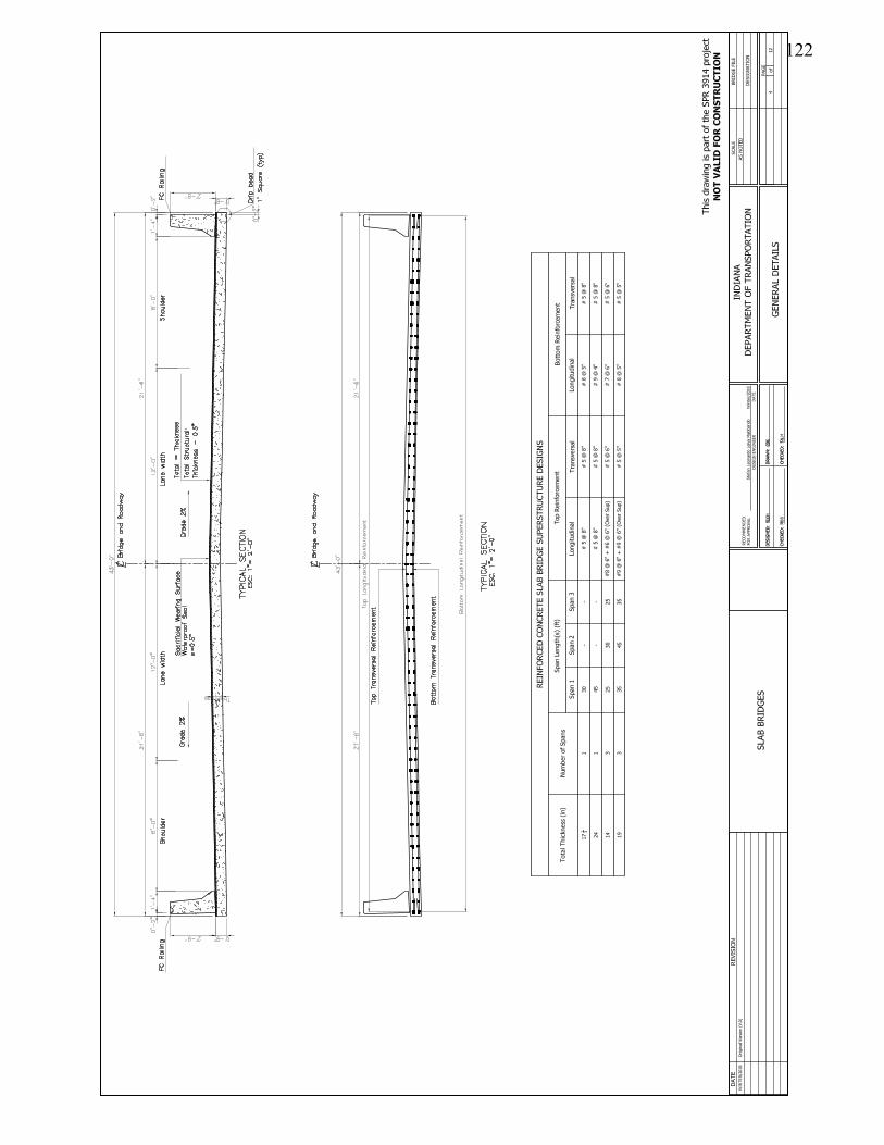
122

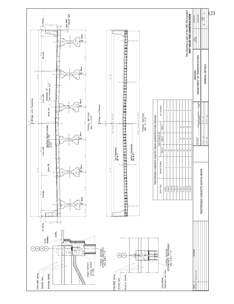
123

124

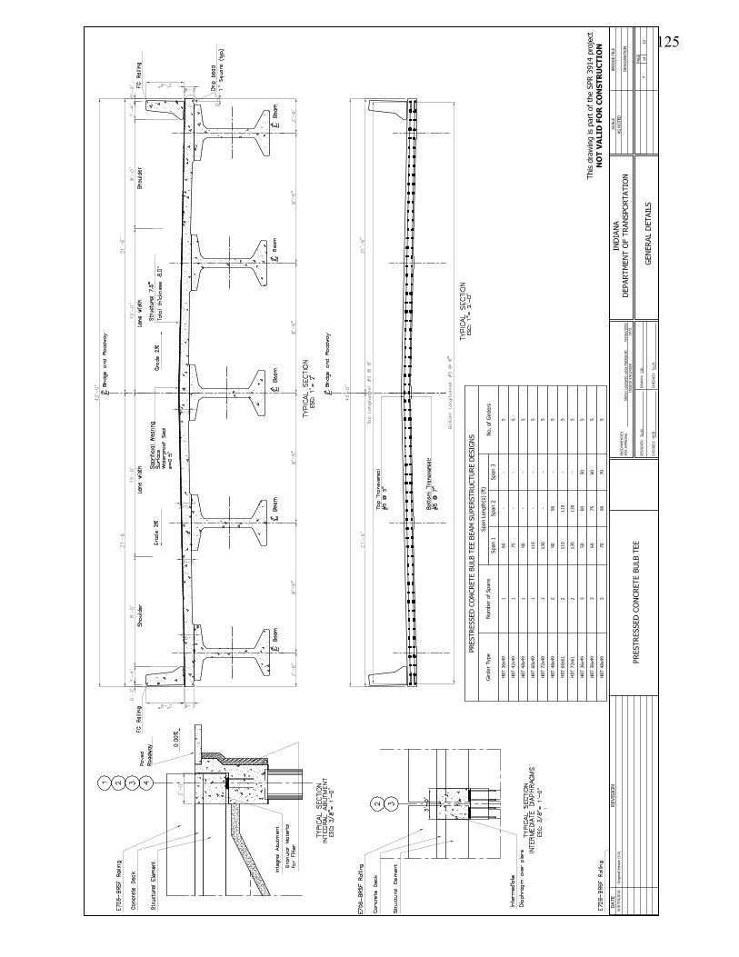
125

126

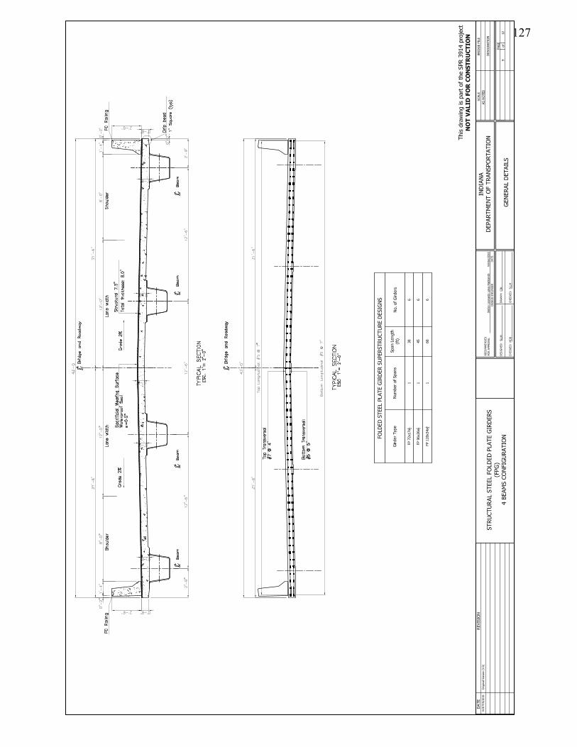
127

128

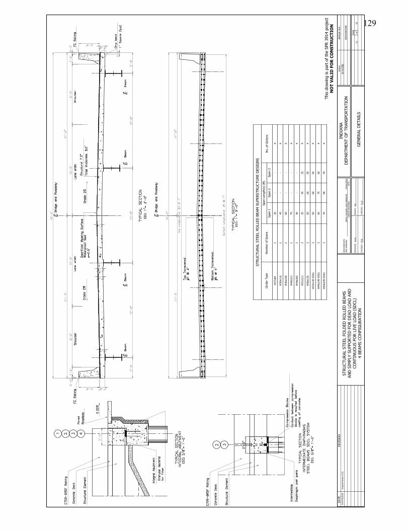
129

130

131

B. BASIC CONCEPTS OF PROBABILITY

The aim of this section is to give definitions of basic concepts of probability that

would be helpful to the reader to better understand the main body of the document.

In addition, definitions of all probability distribution functions used in this study are

summarized.

B.1 The Probabilty Density Function (PDF)

This section is based on the book by Morgan [74]. When F (x) is a continuous

funtion of x, with a continuous first derivative, then f(x) = dF (x)/dx is called the

probability density function of the random variable X. The pdf has the following

properties:

i .

f(x) ≥ 0 (B.1)

ii .∞∫

−∞

f(x)dx = 1 (B.2)

iii .

Pr(a < X < b) = Pr(a ≤ X < b) = Pr(a < X ≤ b) = Pr(a ≤ X ≤ b) (B.3)

=

b∫a

f(x)dx

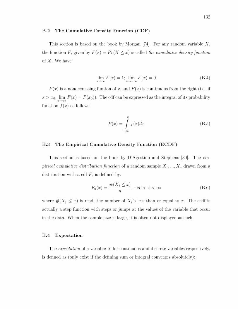
132

B.2 The Cumulative Density Function (CDF)

This section is based on the book by Morgan [74]. For any random variable X,

the function F , given by F (x) = Pr(X ≤ x) is called the cumulative density function

of X. We have:

limx→∞

F (x) = 1; limx→−∞

F (x) = 0 (B.4)

F (x) is a nondecreasing funtion of x, and F (x) is continuous from the right (i.e. if

x > x0, limx→x0

F (x) = F (x0)). The cdf can be expressed as the integral of its probability

function f(x) as follows:

F (x) =

c∫−∞

f(x)dx (B.5)

B.3 The Empirical Cumulative Density Function (ECDF)

This section is based on the book by D’Agostino and Stephens [30]. The em-

pirical cumulative distribution function of a random sample X1, ..., Xn drawn from a

distribution with a cdf F , is defined by:

Fn(x) =#(Xj ≤ x)

n,−∞ < x <∞ (B.6)

where #(Xj ≤ x) is read, the number of Xj’s less than or equal to x. The ecdf is

actually a step function with steps or jumps at the values of the variable that occur

in the data. When the sample size is large, it is often not displayed as such.

B.4 Expectation

The expectation of a variable X for continuous and discrete variables respectively,

is defined as (only exist if the defining sum or integral converges absolutely):

133

E[X] =

∞∫−∞

xf(x)dx if

∞∫−∞

| x | f(x)dx <∞ (B.7)

E[X] =∑i

xiPr(X = xi) if∑i

| xi | Pr(X = xi)x <∞ (B.8)

The variance of a random variable X is defined as:

V ar(X) = E[(X − E[X])2] (B.9)

and the covariance between random variables X and Y is defined as:

Cov(X, Y ) = E[(X − E[X])(Y − E[Y ])] (B.10)

B.5 Useful Probability Distributions

This section presents the probability density functions, cumulative density func-

tion and distribution parameters for each of the distribution mentioned in the main

body of this document. [30] [74] [36] [75] [76]

B.5.1 The Normal distribution

Also known as the Gaussian distribution, it is the most widely used probability

distribution. The parameters used for this distribution are the mean (µ) and the stan-

dard deviation (σ). A short notation for this distribution is N(µ, σ). The probability

density function is as follows:

f(x | µ, σ) =1

σ√

2πe

[− 1

2(x−µσ )2]

(B.11)

and the cumulative density function as:

F (x | µ, σ) =1

σ√

2π

x−µσ∫

−∞

e

[− 1

2(x−µσ )2]

=1

2

[1 + erf

(x− µσ√

2

)](B.12)

134

B.5.2 The Gamma distribution

If the occurrences of an event are considered a Poisson process (i.e. an event can

occur at random at any time or any point in space), then the time until the kth

occurrence of the event is governed by the gamma distribution. This distribution is

also considered as a general purpose pdf. The parameters used for this distribution

are the shape (κ) and the scale (θ, i.e. as the inverse of the mean occurrence rate υ,

υ = 1/θ) parameters. The probability density function is as follows:

f(x | κ, θ) =1

Γ(κ)θκxκ−1e

xθ (B.13)


F (x | κ, θ) =1

Γ(κ)γ(κ,x

θ

)(B.14)

where γ(κ, x

θ

)is defined as the lower incomplete gamma function also known as the

incomplete gamma function ratio. However, there are some events in which the data

skewness is significant. In those cases, a third parameter would be necessary. For

these cases, the shifted gamma distribution, which is a three-parameter distribution,

is useful. The extra parameter is called shift (ω). Then the pdf and the cdf are as

follows:

f(x | κ, θ, ω) =1

Γ(κ)θκ(x− ω)κ−1e

x−ωθ (B.15)

F (x | κ, θ, ω) =1

Γ(κ)γ

(κ,x− ωθ

)(B.16)

B.5.3 The Weibull distribution

It is named after the Swedish mathematician Waloddi Weibull, who described it

in detail in 1951 as a result of his research on strength of materials and fatigue. he

parameters used for this distribution are the shape (κ) and the scale (λ) parameters.

The probability density function is as follows:

f(x | κ, λ) =

κλ

(xλ

)κ−1e−(

xλ)κ x ≥ 0

0 x < 0

(B.17)

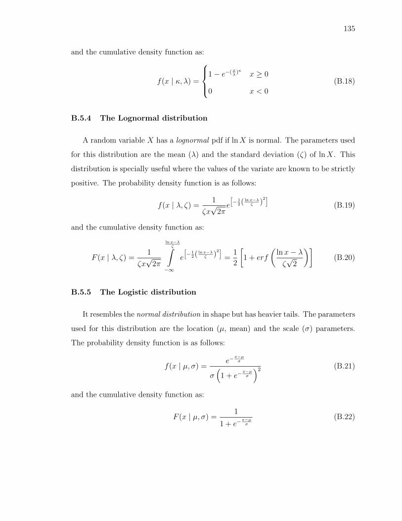
135


f(x | κ, λ) =

1− e−( xλ )κ x ≥ 0

0 x < 0

(B.18)

B.5.4 The Lognormal distribution

A random variable X has a lognormal pdf if lnX is normal. The parameters used

for this distribution are the mean (λ) and the standard deviation (ζ) of lnX. This

distribution is specially useful where the values of the variate are known to be strictly

positive. The probability density function is as follows:

f(x | λ, ζ) =1

ζx√

2πe

[− 1

2( ln x−λζ )

2]

(B.19)


F (x | λ, ζ) =1

ζx√

2π

ln x−λζ∫

−∞

e

[− 1

2( ln x−λζ )

2]

=1

2

[1 + erf

(lnx− λζ√

2

)](B.20)

B.5.5 The Logistic distribution

It resembles the normal distribution in shape but has heavier tails. The parameters

used for this distribution are the location (µ, mean) and the scale (σ) parameters.

The probability density function is as follows:

f(x | µ, σ) =e−

x−µσ

σ(

1 + e−x−µσ

)2 (B.21)


F (x | µ, σ) =1

1 + e−x−µσ

(B.22)

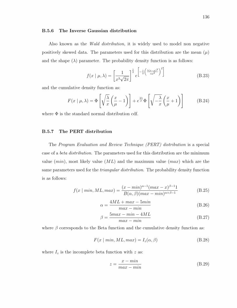
136

B.5.6 The Inverse Gaussian distribution

Also known as the Wald distribution, it is widely used to model non negative

positively skewed data. The parameters used for this distribution are the mean (µ)

and the shape (λ) parameter. The probability density function is as follows:

f(x | µ, λ) =

[1

x3√

2π

] 12

e

[− 1

2

(λ(x−µ)2

xµ2

)2]

(B.23)


F (x | µ, λ) = Φ

[√λ

x

(x

µ− 1

)]+ e

2λµ Φ

[√−λx

(x

µ+ 1

)](B.24)

where Φ is the standard normal distribution cdf.

B.5.7 The PERT distribution

The Program Evaluation and Review Technique (PERT) distribution is a special

case of a beta distribution. The parameters used for this distribution are the minimum

value (min), most likely value (ML) and the maximum value (max) which are the

same parameters used for the triangular distribution. The probability density function

is as follows:

f(x | min,ML,max) =(x−min)α−1(max− x)β−11

B(α, β)(max−min)α+β−1(B.25)

α =4ML+max− 5min

max−min(B.26)

β =5max−min− 4ML

max−min(B.27)

where β corresponds to the Beta function and the cumulative density function as:

F (x | min,ML,max) = Iz(α, β) (B.28)

where Iz is the incomplete beta function with z as:

z =x−min

max−min(B.29)

137

C. LIFE CYCLE PROFILES FOR INDIANA BRIDGES

This appendix presents the different life-cycle cost profiles considered for each one of

the superstructures analyzed in this document. Those presented in Chapter 6 are the

most cost-effective LCCP for each of the superstructure types used.

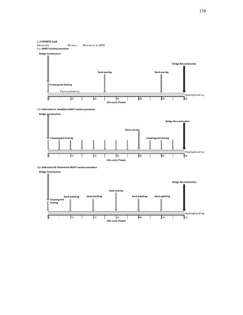
138

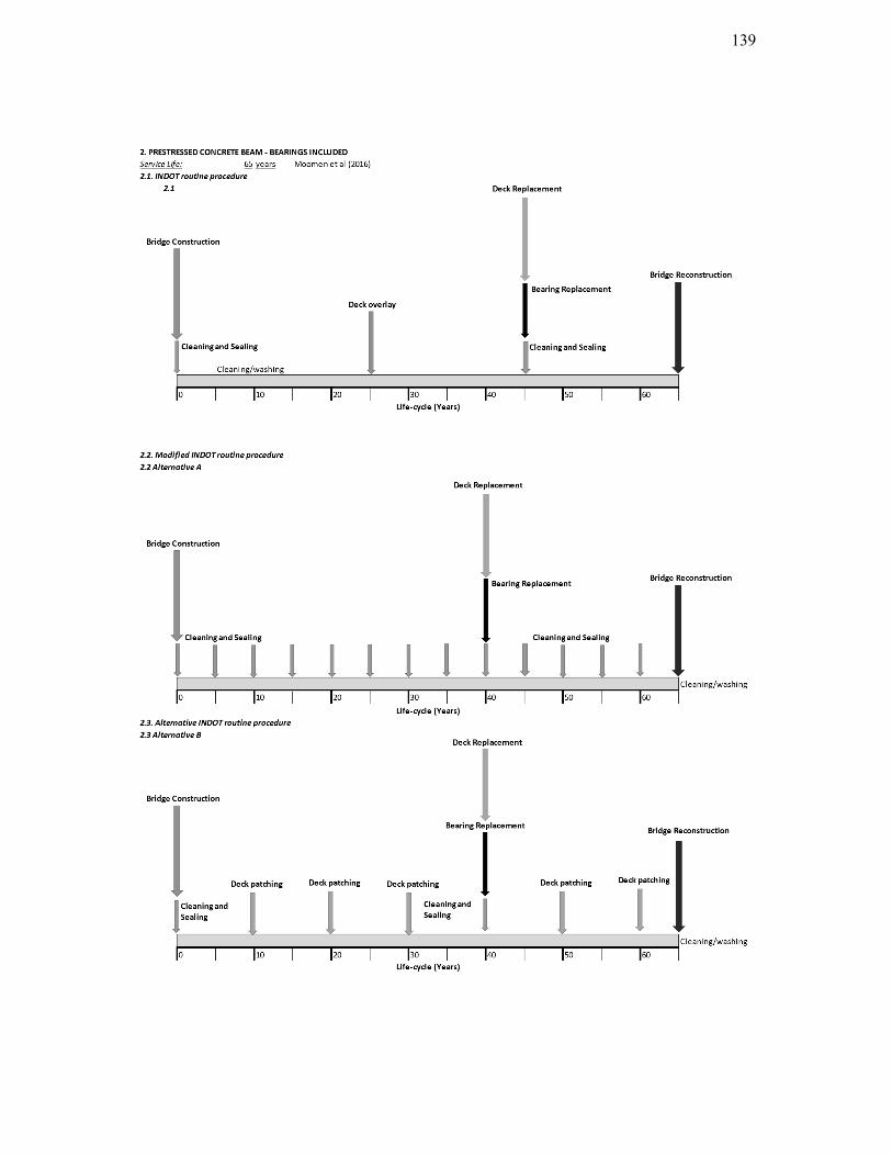
139

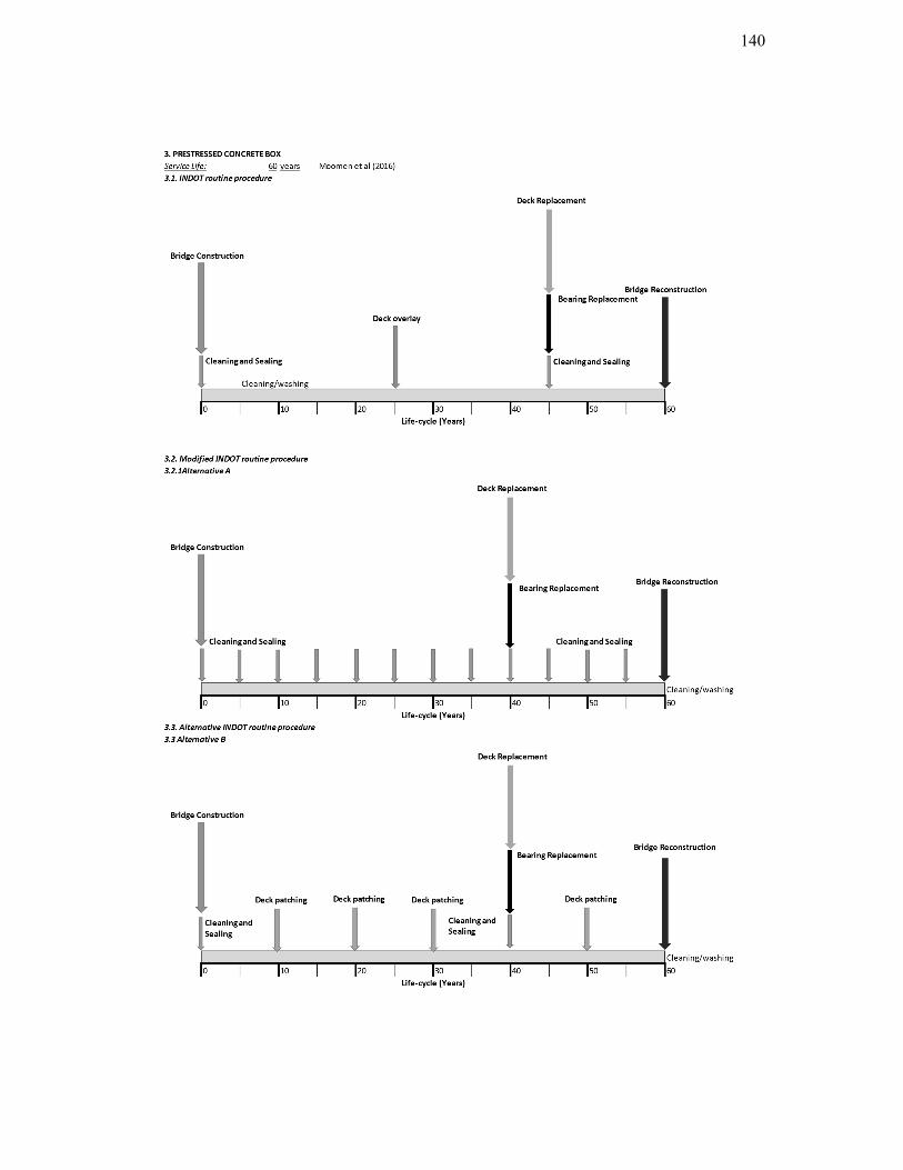
140

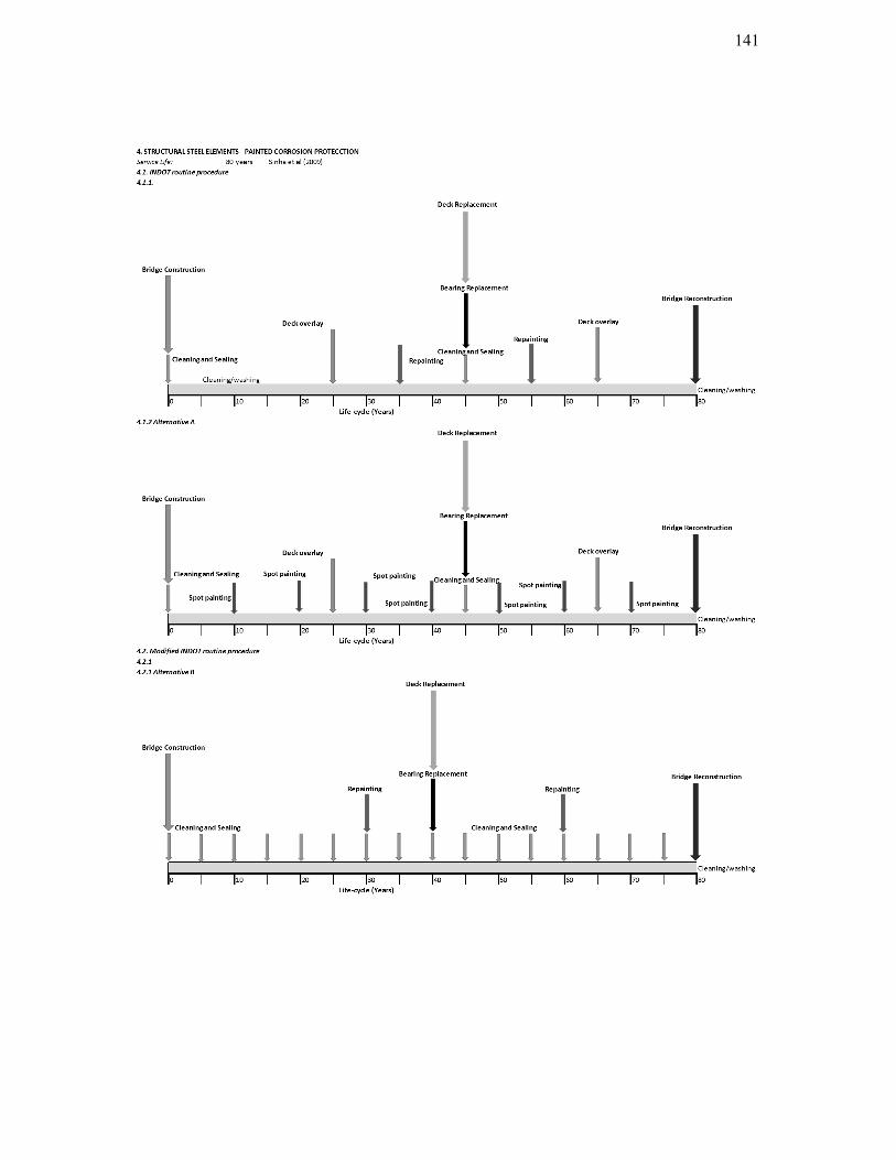
141

142

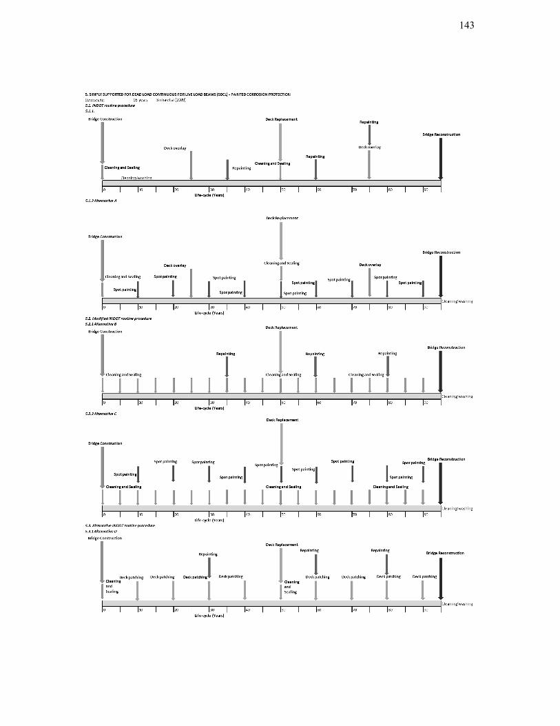
143

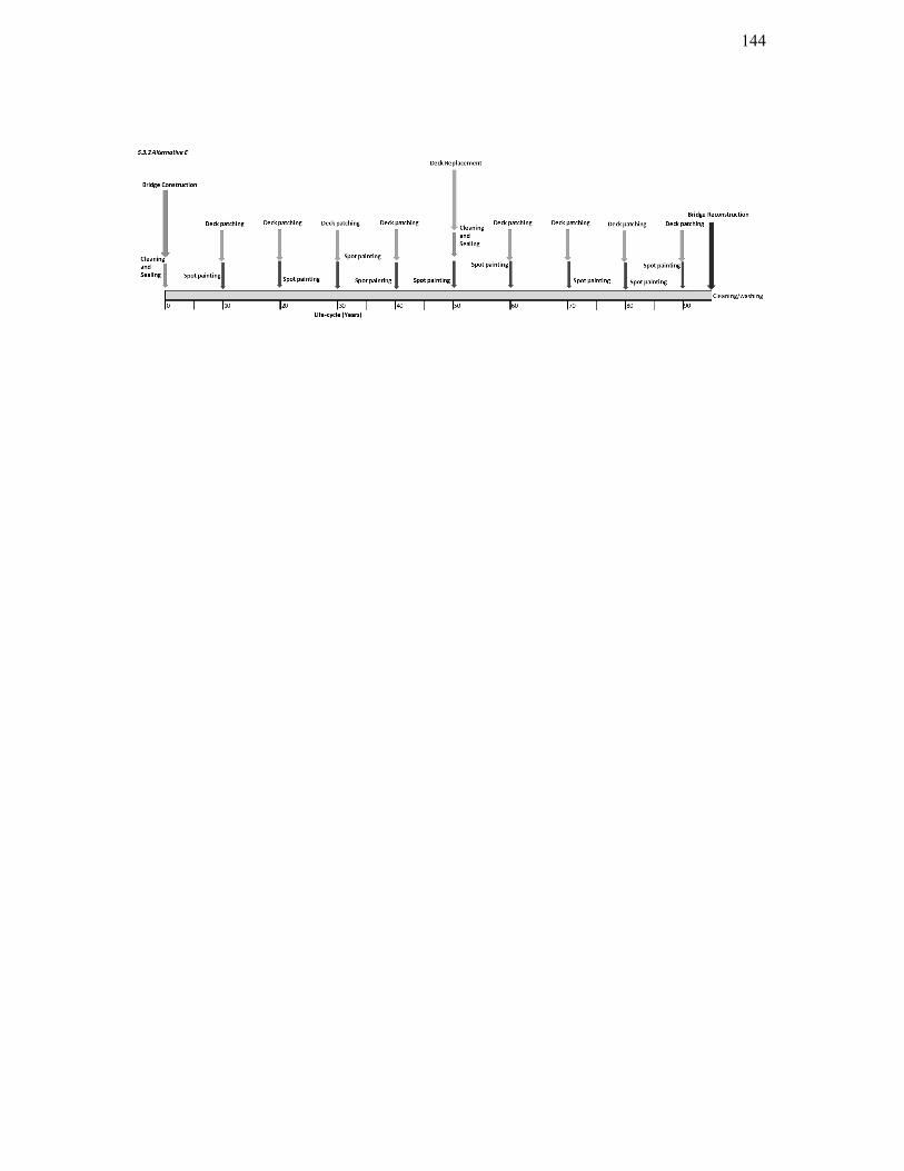
144

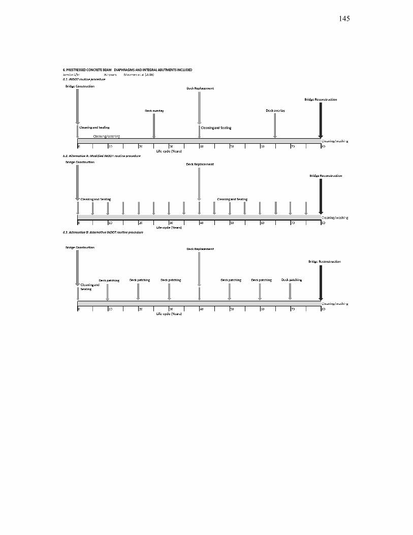
145

146

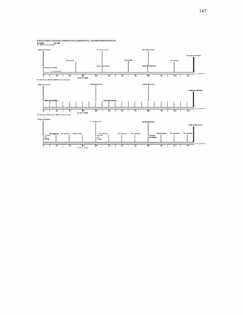
147

148

D. INTEREST EQUATIONS AND EQUIVALENCES

According to Sinha and Labi [64], interest equations known also as equivalency equa-

tions are the relationships between amounts of money that occur at different points

in time and are used to estimate the worth of a single amount of money or a series

of monetary amounts from one time period to another to reflect the time value of

money. All relationships involve some of the following five basic factors: P , initial

amount; F , amount of money at a specified future period; A, a periodic amount of

money; i,the interest rate or discount rate for the compounding period; and N , a

specified number of compounding periods or the analysis period.

D.1 Single Payment Compound Amount Factor (SPACF)

Finding the future compounded amount (F ) at the end of a specified period given

the initial amount (P ), the analysis period (N) and interest rate (i), is given by

Equation D.1.

F = P × SPACF , SPACF = (1 + i)N (D.1)

D.2 Single Payment Present Worth Factor (SPPWF)

Finding the initial amount (P ) that would yield a given future amount (F ), at

the end of an specified analysis period (N) given the interest rate (i), is given by

Equation D.2.

P = F × SPPWF , SPPWF =1

(1 + i)N(D.2)

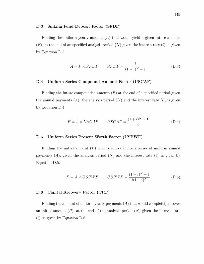
149

D.3 Sinking Fund Deposit Factor (SFDF)

Finding the uniform yearly amount (A) that would yield a given future amount

(F ), at the end of an specified analysis period (N) given the interest rate (i), is given

by Equation D.3.

A = F × SFDF , SFDF =i

(1 + i)N − 1(D.3)

D.4 Uniform Series Compound Amount Factor (USCAF)

Finding the future compounded amount (F ) at the end of a specified period given

the annual payments (A), the analysis period (N) and the interest rate (i), is given

by Equation D.4.

F = A× USCAF , USCAF =(1 + i)N − 1

i(D.4)

D.5 Uniform Series Present Worth Factor (USPWF)

Finding the initial amount (P ) that is equivalent to a series of uniform annual

payments (A), given the analysis period (N) and the interest rate (i), is given by

Equation D.5.

P = A× USPWF , USPWF =(1 + i)N − 1

i(1 + i)N(D.5)

D.6 Capital Recovery Factor (CRF)

Finding the amount of uniform yearly payments (A) that would completely recover

an initial amount (P ), at the end of the analysis period (N) given the interest rate

(i), is given by Equation D.6.

150

A = P × CRF , CRF =(i(1 + i)N)

(1 + i)N − 1(D.6)

151

E. EXAMPLE OF LIFE-CYCLE COST ANALYSIS -

DETERMINISTIC APPROACH

This section describes the procedure used for the computation of the LCCA and the

indicator of economic efficiency. Information needed is the following: Alternatives

considered, bridge designs, service life depending on the superstructure type, life-

cycle profiles and working action scheduling, agency costs and finally, the LCCA

strategy including discount rate and comparison criteria as mentioned earlier in this

Appendix.

As a general outline, this example is performed using the following procedure.

First, computation of the initial cost for all the alternatives is assembled. Then a

LCCA of different profiles for one superstructure alternative is conducted to show the

procedure used for the selection of the definitive profile. After that, computation of

the LCCA for the different superstructure type alternatives is done, followed by the

estimation of the LCCAP of each one of them.

Following the design plan shown in Chapter 3, six different superstructure types

are considered for the simply supported configuration in span range 1, and specif-

ically for a span length of 30-ft. Types considered are the following: slab bridge,

structural steel rolled beam bridge (5 beams configuration alternative), structural

steel rolled beam bridge (4 beams configuration alternative), prestressed concrete

AASHTO beams bridge, structural steel FPG bridge, and prestressed concrete box

beam bridge. As mentioned before in this document, barriers and other miscellaneous

elements are not considered in the initial cost estimation. Thus, the only costs consid-

ered are those for concrete for the superstructure (slab), reinforcing steel, structural

steel, and prestressed concrete elements. The costs used are shown in Tables 4.2 to

4.4 and .Quantities were obtained from the designs drawings shown in the Appendix

A. Critical features for each of the designs alternatives are noted below:

152

• Slab bridge: Total concrete slab thickness of 17.5-in including sacrificial surface.

Longitudinal reinforcing steel (parallel to direction of the traffic): #5 @ 8 top

and #8 @ 5 bottom. Transverse reinforcing steel (perpendicular to direction of

the traffic): #5 @ 8.0 top and bottom.

• Structural steel rolled beams (5 beams): Total concrete slab thickness of 8.0-

in including sacrificial surface. Transverse reinforcing steel (perpendicular to

direction of the traffic): #7 @ 5.0 top and #5 @ 7.0 bottom. Longitudinal

reinforcing steel (parallel to direction of the traffic): #5 @ 7.0 top and bottom.

Five (5) W18x65 beams separated by 9.5-ft.

• Structural steel rolled beams (4 beams): Total concrete slab thickness of 8.0-

in including sacrificial surface. Transverse reinforcing steel (perpendicular to

direction of the traffic): #7 @ 4.0 top and #5 @ 5.0 bottom. Longitudinal

reinforcing steel (parallel to direction of the traffic): #5 @ 7 top and bottom.

Four (4) W18x76 beams separated by 12.5-ft.

• Prestressed concrete AASTHO beams: Total concrete slab thickness of 8.0-in

including sacrificial surface. Transverse reinforcing steel (perpendicular to direc-

tion of the traffic): #5 @ 4.0 top and #5 @ 8.0 bottom. Longitudinal reinforcing

steel (parallel to direction of the traffic): #5 @ 8.0 top and bottom. Six (6) type

I AASHTO beams separated by 7.5-ft.

• Structural steel FPG (6 beams): Total concrete slab thickness of 8.0-in including

sacrificial surface. Transverse reinforcing steel (perpendicular to direction of

the traffic): #5 @ 5.0 top and #5 @ 8.0 bottom. Longitudinal reinforcing

steel (parallel to direction of the traffic): #5 @ 8.0 top and bottom. Six (6)

FP60x12x1/2 beams separated by 7.5-ft.

• Structural steel FPG (4 beams): Total concrete slab thickness of 8.0-in including

sacrificial surface. Transverse reinforcing steel (perpendicular to direction of

the traffic): #7 @ 4.0 top and #5 @ 5.0 bottom. Longitudinal reinforcing

153

steel (parallel to direction of the traffic): #5 @ 7.0 top and bottom. Six (4)

FP72x17x1/2 beams separated by 12.5-ft.

• Prestressed concrete box beams: Total concrete slab thickness of 8.0-in including

sacrificial surface. Transverse reinforcing steel (perpendicular to direction of the

traffic): #5 @ 5.0 top and #5 @ 7.0 bottom. Longitudinal reinforcing steel

(parallel to direction of the traffic): #5 @ 8.0 top and bottom. Five (5) box

beams CB17x48 separated by 9.5-ft.

Based on the descriptions of the design features for each of the alternatives, the

construction costs can be obtained. The initial cost for all the alternatives is shown

in Table E.1. Since the construction is considered at year 0, this value does not

need to be discounted to a present value. However, if Equation 7.1 is to be used to

calculate the LCCA, present values will be used to compute the single life-cycle cost

of the alternative, then this amount is projected to the end of the service life using

the SPACF, and finally the LCCAP is obtained (Equation 7.1).

Table E.1.Initial cost Simply supported beam, span 30 ft.

Span (ft) Superstructure Type Width (ft) Total Cost ($)

30

Slab Bridge 43 51,438

Steel Beam Painted (4 Beams) 43 59,464

Steel Beam Painted (5 Beams) 43 59,224

Steel Beam Galvanized (4 Beams) 43 62,511

Steel Beam Galvanized (5 Beams) 43 62,234

PS Concrete AASHTO Beam (Bearings) 43 59,747

PS Concrete AASHTO Beam (Diaph) 43 73,639

Steel FPG Galvanized (6 Beams) 43 67,921

Steel FPG Galvanized (4 Beams) 43 62,790

PS Concrete Box Beams 43 75,404

Life-cycle profile selection and TLCC estimation

Different maintenance schedules were considered for each superstructure type that resulted

in different life-cycle profiles. The minimum TLCC among all the different alternatives per

superstructure type is then used for comparison with other superstructure types. Therefore, the

lowest value corresponds to the most cost effective option for that specific span length. All the

different profiles used can be seen in Appendix D. For this illustrative example, only one

superstructure type is detailed (slab bridge). For the remaining types only the most cost-effective

profile is shown.

Working actions considered for the slab bridges are described below, various combinations

of all of them are presented in the life-cycle profiles shown in Figure 1.

• Cleaning and washing of the deck: Only the current INDOT practice is taken into

account. The procedure is performed on a yearly basis.

• Deck Overlay: Two different alternatives were considered: Alternative A involves

a first overlay after 25 years of original construction, then a 25 years of overlay

service life. Due to the limited service life of this type of superstructure, only two

overlays are considered. However, INDOT policies indicates that a slab bridge

could stand up to three different overlays if needed until the end of its service life.

Alternative B involves a single overlay after 40 years of construction along with a

process of sealing and cleaning of the deck surface every 5 years.

• Sealing and cleaning of the deck surface: INDOT current policy contemplate the

sealing and cleaning of the deck surface only after the construction/reconstruction

of the deck, it means it is considered at year 0 exclusively for slab bridges.

154

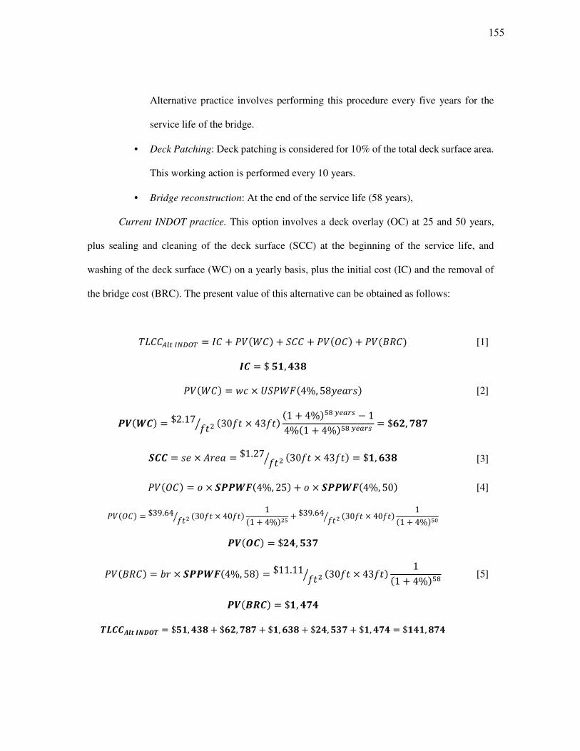
Alternative practice involves performing this procedure every five years for the

service life of the bridge.

• Deck Patching: Deck patching is considered for 10% of the total deck surface area.

This working action is performed every 10 years.

• Bridge reconstruction: At the end of the service life (58 years),

Current INDOT practice. This option involves a deck overlay (OC) at 25 and 50 years,

plus sealing and cleaning of the deck surface (SCC) at the beginning of the service life, and

washing of the deck surface (WC) on a yearly basis, plus the initial cost (IC) and the removal of

the bridge cost (BRC). The present value of this alternative can be obtained as follows:

�� = �� + �� + �� + �� + �� [1]

�� = $��, � !

�� = "# × %��&�4%, 58+,-./� [2]

01�2�� = $2.17 789: �3078 × 4378� �1 + 4%�=>?@ABC − 14%�1 + 4%�=>?@ABC = $EF, G!G

H�� = /, × I.,- = $1.27 789: �3078 × 4378� = $�, E ! [3]

�� = J × H002K�4%, 25� + J × H002K�4%, 50� [4]

�� = $39.64 789: �3078 × 4078� 1�1 + 4%�9= + $39.64 789: �3078 × 4078� 1�1 + 4%�=N

01�O�� = $F�, � G

�� = P. × H002K�4%, 58� = $11.11 789: �3078 × 4378� 1�1 + 4%�=> [5]

01�QR�� = $�, �G�

ST��UVW�XYOS = $��, � ! + $EF, G!G + $�, E ! + $F�, � G + $�, �G� = $��, !G�

155

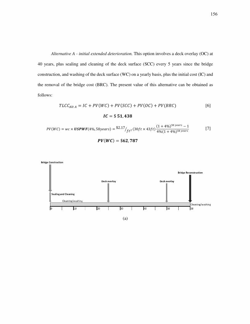
Alternative A - initial extended deterioration. This option involves a deck overlay (OC) at

40 years, plus sealing and cleaning of the deck surface (SCC) every 5 years since the bridge

construction, and washing of the deck surface (WC) on a yearly basis, plus the initial cost (IC) and

the removal of the bridge cost (BRC). The present value of this alternative can be obtained as

follows:

�� = �� + �� + �� + �� + �� [6]

�� = $��, � !

�� "# $ ZH02K�4%, 58+,-./� $2.17 789: �3078 $ 4378� �1 � 4%�=>?@ABC D 14%�1 � 4%�=>?@ABC [7]

01�2�� $EF, G!G

(a)

156

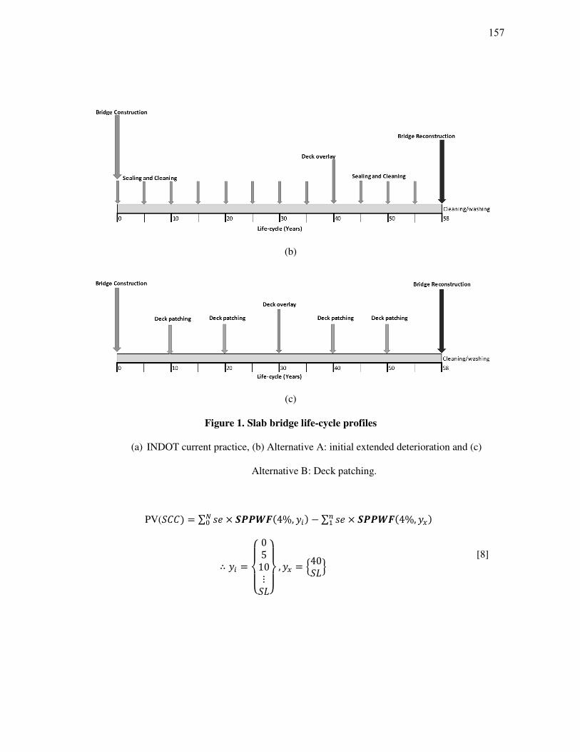
(b)

(c)

Figure 1. Slab bridge life-cycle profiles

(a) INDOT current practice, (b) Alternative A: initial extended deterioration and (c)

Alternative B: Deck patching.

PV(�� = ∑ /, × H002K�4%, +\�N D ∑ /, $ H002K�4%, +]�_

∴ +\ abcbd 0510⋮��fbg

bh , +] i40��j [8]

157

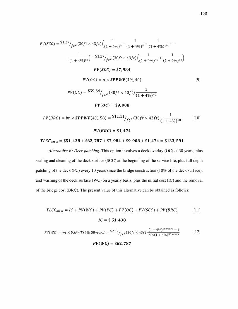
�� = $1.27 789: �3078 × 4378� k 1�1 + 4%�N + 1�1 + 4%�= + 1�1 + 4%�_N +⋯+ 1�1 + 4%�=>m − $1.27 789: �3078 × 4378� k 1�1 + 4%�nN + 1�1 + 4%�=>m

01�H�� = $G, o!�

�� = J × H002K�4%, 40� [9]

�� = $39.64 789: �3078 × 4078� 1�1 + 4%�nN

01�O�� = $o, op!

�� = P. × H002K�4%, 58� = $11.11 789: �3078 × 4378� 1�1 + 4%�=> [10]

01�QR�� = $�, �G�

ST��UVWU = $��, � ! + $EF, G!G + $G, o!� + $o, op! + $�, �G� = $� , �o�

Alternative B: Deck patching. This option involves a deck overlay (OC) at 30 years, plus

sealing and cleaning of the deck surface (SCC) at the beginning of the service life, plus full depth

patching of the deck (PC) every 10 years since the bridge construction (10% of the deck surface),

and washing of the deck surface (WC) on a yearly basis, plus the initial cost (IC) and the removal

of the bridge cost (BRC). The present value of this alternative can be obtained as follows:

��q = �� + �� + �� + �� + �� + �� [11]

�� = $��, � !

�� = "# × %��&�4%, 58+,-./� = $2.17 789: �3078 × 4378� �1 + 4%�=>?@ABC − 14%�1 + 4%�=>?@ABC [12]

01�2�� = $EF, G!G

158

PV(�� = ∑ r# × H002K�4%, +\�_ − ∑ r# × H002K�4%, +]�_

∴ +\ = s1020⋮��t , +] = i30��j [13]

�� = $37.23 789: �3078 × 4078� × 10%k 1�1 + 4%�_N + 1�1 + 4%�9N +⋯+ 1�1 + 4%�=>m− $37.23 789: �3078 × 4078� × 10% k 1�1 + 4%�uN + 1�1 + 4%�=>m

01�0�� = $E, E�E

�� = /, × I.,- = $1.27 789: �3078 × 4378� = $�, E ! [14]

�� = J × H002K�4%, 30� [15]

�� = $39.64 789: �3078 × 4078� 1�1 + 4%�uN

01�O�� = $��, EEE

�� = P. × H002K�4%, 58� = $11.11 789: �3078 × 4378� 1�1 + 4%�=> [16]

01�QR�� = $�, �G�

ST��UVWQ = $��, � ! + $EF, G!G + $��, EEE + $E, E�E + �, E ! + $�, �G�

ST��UVWQ = $� E, o!�

As it can be seen, no residual value or salvage value was included. Salvage value was only

considered for the steel superstructures and it was included as a benefit. To conclude, it is shown

that the most cost-effective profile for slab bridges corresponds to Alternative B.

Following the same principles for the remaining superstructure types, the most cost-

effective life-cycle profiles were chosen. However, only the calculation of the definitive profiles

159

for each of the superstructure types analyzed are shown below. Refer to Appendix D for all life-

cycle profiles considered for all superstructure types.

Structural Steel Rolled Beam – 5 Beam Configuration: Alternative C: Bearing

replacement, spot painting and sealing process. This option involves a deck reconstruction (DRC)

at 40 years, plus sealing and cleaning of the deck surface (SCC) every 5 years since the bridge

construction, plus spot painting (SPC) every 10 years since the bridge construction (10% of the

structural element surface),bearing replacements (BC) at 40 years, and washing of the deck surface

(WC) on a yearly basis, plus the initial cost (IC), the removal of the bridge cost (BRC) and the

salvage value represented by the benefit of selling the structural steel for recycling (SRC). In

addition, some details are needed regarding the structural steel beam elements. Firstly, the exposed

perimeter of the beam is for spot painting 4.94 ft. Secondly, the total weight of the steel elements

is 10,506 lb. Finally, a total price for the reinforcement steel of $12,365 which will be included

together with the bridge deck reconstruction cost calculation. The present value of this alternative

can be obtained as follows:

��v = �� + �� + �� + ��w�� + �� + �� + �� + �� [17]

�� = $�o, �E�

�� = "# × %��&�4%, 80+,-./� = $2.17 789: �3078 × 4378� �1 + 4%�>N?@ABC − 14%�1 + 4%�>N?@ABC [18]

01�2�� = $EE, o�E

PV(�� = ∑ /, × H002K�4%, +\�N − ∑ /, × H002K�4%, +]�_

∴ +\ = abcbd 0510⋮��fbg

bh , +] = x��y [19]

160

�� = $1.27 789: �3078 × 4378� k 1�1 + 4%�N + 1�1 + 4%�= + 1�1 + 4%�_N +⋯+ 1�1 + 4%�>Nm − $1.27 789: �3078 × 4378� k 1�1 + 4%�>Nm

01�H�� = $!, !p�

PV(w�� = z. × H002K�4%, 40� [20]

��w�� = k$47.41 789: �3078 × 4378� + $12,365m 1�1 + 4%�nN

01�YR�� = $��, ��

�� = P# × H002K�4%, 40� [21]

�� = $3,483 {|8: �5P} × 2/{r� 1�1 + 4%�nN

01�Q�� = $G, F��

PV(SP�� = ∑ /r# × H002K�4%, +\�N − ∑ /r# × H002K�4%, +]�_ [22]

∴ +\ = abcbd102030⋮��fbg

bh , +] = x��y

�� = $2.19 789: �4.9478 × 3078 × 5P} × 10%� k 1�1 + 4%�_N + 1�1 + 4%�9N +⋯+ 1�1 + 4%�>Nm − $1.27 789: �4.9478 × 3078 × 5P} × 10%� k 1�1 + 4%�>Nm

01�H0�� = $ �E

�� = P. × H002K�4%, 80� = $11.11 789: �3078 × 4378� 1�1 + 4%�>N [23]

01�QR�� = $EFF

�� = /. × H002K�4%, 80� = $0.08 �P: �5 × 10,506~P� 1�1 + 4%�>N [24]

161

01�HR�� = $�!F

ST��UVW� = $�o, �E� + $EE, o�E + $!, !p� + $��, �� + $G, F�� + $ �E + $EFF − $�!F

ST��UVW� = $��!, � �

Prestressed Concrete AASTHO Beams: Alternative A –modified INDOT routine

procedure. This option involves a deck reconstruction (DRC) at 40 years, plus sealing and cleaning

of the deck surface (SCC) every 5 years since the bridge construction, bearing replacements (BC)

at 45 years, and washing of the deck surface (WC) on a yearly basis, plus the initial cost (IC) and

the removal of the bridge cost (BRC). Finally, a total price for the reinforcing steel of $9,086 which

will be included together with the bridge deck reconstruction cost calculation. The present value

of this alternative can be obtained as follows:

�� = �� + �� + �� + ��w�� + �� + �� [25]

�� = $�o, G�G

�� = "# × ZH02K�4%,65+,-./� = $2.17 789: �3078 × 4378� �1 + 4%��=?@ABC − 14%�1 + 4%��=?@ABC [26]

01�2�� = $E�, ��

PV(�� = ∑ /, × H002K�4%, +\�N − ∑ /, × H002K�4%, +]�_

∴ +\ = abcbd 0510⋮��fbg

bh , +] = x��y [27]

�� = $1.27 789: �3078 × 4378� k 1�1 + 4%�N + 1�1 + 4%�= + 1�1 + 4%�_N +⋯+ 1�1 + 4%��=m − $1.27 789: �3078 × 4378� k 1�1 + 4%��=m

162

01�H�� = $!, �!�

PV(w�� = z. × H002K�4%, 40� [28]

��w�� = k$47.41 789: �3078 × 4378� + $9,086m 1�1 + 4%�nN

01�YR�� = $��, E �

�� = P# × H002K�4%, 40� [29]

�� = $3,483 {|8: �6P} × 2/{r� 1�1 + 4%�nN

01�Q�� = $!, Gp�

�� = P. × H002K�4%, 65� = $11.11 789: �3078 × 4378� 1�1 + 4%��= [30]

01�QR�� = $�, �Fp

ST��UVWU = $�o, G�G + $E�, �� + $!, �!� + $��, E � + $!, Gp� + $�, �Fp

ST��UVWU = $��G, �oo

Structural Steel Rolled Beam – 4 Beam Configuration: Alternative C: Bearing

replacement, spot painting and sealing process. This option involves a deck reconstruction (DRC)

at 40 years, plus sealing and cleaning of the deck surface (SCC) every 5 years since the bridge

construction, plus spot painting (SPC) every 10 years since the bridge construction (10% of the

structural element surface),bearing replacements (BC) at 40 years, and washing of the deck surface

(WC) on a yearly basis, plus the initial cost (IC), the removal of the bridge cost (BRC) and the

salvage value represented by the benefit of selling the structural steel for recycling (SRC). In

addition, some details are needed regarding the structural steel beam elements. Firstly, the exposed

perimeter of the beam is 5.76 ft. Secondly, the total weight of the steel elements is 10,382 lb.

Finally, a total price for the reinforcement steel of $14,222 which will be included together with

163

the bridge deck reconstruction cost calculation. The present value of this alternative can be

obtained as follows:

��v = �� + �� + �� + ��w�� + �� + ��+ �� + �� [31]

�� = $�o, FF�

�� = "# × ZH02K�4%, 80+,-./� = $2.17 789: �3078 × 4378� �1 + 4%�>N?@ABC − 14%�1 + 4%�>N?@ABC [32]

01�2�� = $EE, o�E

PV(�� = ∑ /, × H002K�4%, +\�N − ∑ /, × H002K�4%, +]�_

∴ +\ = abcbd 0510⋮��fbg

bh , +] = x��y [33]

�� = $1.27 789: �3078 × 4378� k 1�1 + 4%�N + 1�1 + 4%�= + 1�1 + 4%�_N +⋯+ 1�1 + 4%�>Nm − $1.27 789: �3078 × 4378� k 1�1 + 4%�>Nm

01�H�� = $!, !p�

PV(w�� = z. × H002K�4%, 40� [34]

��w�� = k$47.41 789: �3078 × 4378� + $14,222m 1�1 + 4%�nN

01�YR�� = $��, Gp�

�� = P# × H002K�4%, 40� [35]

�� = $3,483 {|8: �4P} × 2/{r� 1�1 + 4%�nN

01�Q�� = $�, !p

164

PV(SP�� = ∑ /r# × H002K�4%, +\�N − ∑ /r# × H002K�4%, +]�_

∴ +\ = abcbd102030⋮��fbg

bh , +] = x��y [36]

�� = $2.19 789: �5.7678 × 3078 × 4P} × 10%� k 1�1 + 4%�_N + 1�1 + 4%�9N +⋯+ 1�1 + 4%�>Nm − $1.27 789: �5.1678 × 3078 × 4P} × 10%� k 1�1 + 4%�>Nm

01�H0�� = $Fo�

�� = P. × H002K�4%, 80� = $11.11 789: �3078 × 4378� �� + 4%�!p [37]

01�QR�� = $EFF

�� = /. × H002K�4%, 80� = $0.08 �P: �4P} × 10,382~P� 1�1 + 4%�>N [38]

01�HR�� = $��

ST��UVW� = $�o, FF� + $EE, o�E + $!, !p� + $��, Gp� + $�, !p + $Fo� + $EFF − $��

ST��UVW� = $��G, F�!

Prestressed Concrete Box Beams: Alternative A – modified INDOT routine procedure.

This option involves a deck reconstruction (DRC) at 40 years, plus sealing and cleaning of the

deck surface (SCC) every 5 years since the bridge construction, bearing replacements (BC) at 40

years, washing of the deck surface (WC) on a yearly basis, plus the initial cost (IC) and the removal

of the bridge cost (BRC). Finally, a total price for the reinforcement steel of $8,651 which will be

included together with the bridge deck reconstruction cost calculation. The present value of this

alternative can be obtained as follows:

165

�� = �� + �� + �� + �� + ��w�� + �� [39]

�� = $G�, �p�

�� = "# × ZH02K�4%, 60+,-./�= $2.17 789: �3078 × 4378� �1 + 4%��N?@ABC − 14%�1 + 4%��N?@ABC

[40]

01�2�� = $E , p

PV(�� = ∑ /, × H002K�4%, +\�N − ∑ /, × H002K�4%, +]�_

∴ +\ = abcbd 0510⋮��fbg

bh , +] = x��y [41]

�� = $1.27 789: �3078 × 4378� k 1�1 + 4%�N + 1�1 + 4%�= + 1�1 + 4%�_N +⋯+ 1�1 + 4%��Nm − $1.27 789: �3078 × 4378� k 1�1 + 4%��Nm

01�H�� = $!, FE

PV(w�� = z. × H002K�4%, 40� [42]

��w�� = k$47.41 789: �3078 × 4378� + $8,651m 1�1 + 4%�nN

01�YR�� = $��, ��

�� = P# × H002K�4%, 30� [43]

�� = $3,483 {|8: �5P} × 2/{r� 1�1 + 4%�nN

01�Q�� = $G, F��

�� = P. × H002K�4%, 60� = $11.11 789: �3078 × 4378� 1�1 + 4%��N [44]

01�QR�� = $�, EF

166

ST��UVWU = $G�, �p� + $E , p + $!, FE + $��, �� + $G, F�� + $�, EF

ST��UVWU = $�Gp, F�G

Structural Steel Rolled Beam – 5 Beam Configuration Galvanized: Alternative A: Bearing

replacement and sealing process. This option involves a deck reconstruction (DRC) at 50 years,

plus sealing and cleaning of the deck surface (SCC) every 5 years since the bridge construction,

bearing replacements (BC) at 50 years, and washing of the deck surface (WC) on a yearly basis,

plus the initial cost (IC), the removal of the bridge cost (BRC) and the salvage value represented

by the benefit of selling the structural steel for recycling (SRC). Structural steel beam elements

with an exposed perimeter of 4.94 ft. and a total weight of the steel elements of 10,506 lb. Finally,

a total price for the reinforcement steel of $12,365 which will be included together with the bridge

deck reconstruction cost calculation. The present value of this alternative can be obtained as

follows:

�� = �� + �� + �� + ��w�� + �� + �� + �� [45]

�� = $EF, ��

�� = "# × ZH02K�4%, 100+,-./�= $2.17 789: �3078 × 4378� �1 + 4%�_NN?@ABC − 14%�1 + 4%�_NN?@ABC

[46]

01�2�� = $E!, �oG

167

PV(�� = ∑ /, × H002K�4%, +\�N − ∑ /, × H002K�4%, +]�_

∴ +\ = abcbd 0510⋮��fbg

bh , +] = x��y [47]

�� = $1.27 789: �3078 × 4378� k 1�1 + 4%�N + 1�1 + 4%�= + 1�1 + 4%�_N +⋯+ 1�1 + 4%�_NNm − $1.27 789: �3078 × 4378� k 1�1 + 4%�_NNm

01�H�� = $o, p�!

PV(w�� = z. × H002K�4%, 50� [48]

��w�� = k$47.41 789: �3078 × 4378� + $12,365m 1�1 + 4%�=N

01�YR�� = $�p, �E

�� = P# × H002K�4%, 50� [49]

�� = $3,483 {|8: �5P} × 2/{r� 1�1 + 4%�=N

01�Q�� = $�, op�

�� = P. × H002K�4%, 100� = $11.11 789: �3078 × 4378� 1�1 + 4%�_NN [50]

01�QR�� = $F!�

�� = /. × H002K�4%, 100� = $0.08 �P: �5 × 10,506~P� 1�1 + 4%�_NN [51]

01�HR�� = $!

ST��UVWU = $EF, �� + $E!, �oG + $o, p�! + $�p, �E + $�, op� + $F!� − $!

ST��UVWU = $��, �G

168

Prestressed Concrete AASTHO Beams Diaphragms Included: Alternative A – Modified

INDOT procedure. This option involves a deck reconstruction (DRC) at 40 years, plus sealing and

cleaning of the deck surface (SCC) every 5 years since the bridge construction, and washing of the

deck surface (WC) on a yearly basis, plus the initial cost (IC) and the removal of the bridge cost

(BRC). Finally, a total price for the reinforcement steel of $9,086 which will be included together

with the bridge deck reconstruction cost calculation. The present value of this alternative can be

obtained as follows:

�� = �� + �� + �� + ��w�� + �� [52]

�� = $G , E o

�� = "# × ZH02K�4%, 80+,-./�= $2.17 789: �3078 × 4378� �1 + 4%�>N?@ABC − 14%�1 + 4%�>N?@ABC

[53]

01�2�� = $EE, o�E

PV(�� = ∑ /, × H002K�4%, +\�N − ∑ /, × H002K�4%, +]�_

∴ +\ = abcbd 0510⋮��fbg

bh , +] = x��y [54]

�� = $1.27 789: �3078 × 4378� k 1�1 + 4%�N + 1�1 + 4%�= + 1�1 + 4%�_N +⋯+ 1�1 + 4%�>Nm − $1.27 789: �3078 × 4378� k 1�1 + 4%�>Nm

01�H�� = $!, !p�

PV(w�� = z. × H002K�4%, 40� [55]

169

��w�� = k$47.41 789: �3078 × 4378� + $9,086m 1�1 + 4%�nN

01�YR�� = $��, E �

�� = P. × H002K�4%, 80� = $11.11 789: �3078 × 4378� �� + 4%�!p [56]

01�QR�� = $EFF

ST��UVWU = $G , E o + $EE, o�E + $!, !p� + $��, E � + $EFF = $�E�, E o

Structural Steel Rolled Beam – 4 Beam Configuration Galvanized: Alternative A: Bearing

replacement and sealing process. This option involves a deck reconstruction (DRC) at 50 years,

plus sealing and cleaning of the deck surface (SCC) every 5 years since the bridge construction,

bearing replacements (BC) at 50 years, and washing of the deck surface (WC) on a yearly basis,

plus the initial cost (IC), the removal of the bridge cost (BRC) and the salvage value represented

by the benefit of selling the structural steel for recycling (SRC). Structural steel beam elements

with an exposed perimeter of 5.76 ft. and a total weight of the steel elements of 10,382 lb. Finally,

a total price for the reinforcement steel of $14,222 which will be included together with the bridge

deck reconstruction cost calculation. The present value of this alternative can be obtained as

follows:

�� = �� + �� + �� + ��w�� + �� + �� + �� [57]

�� = $EF, F �

�� = "# × ZH02K�4%, 100+,-./�= $2.17 789: �3078 × 4378� �1 + 4%�_NN?@ABC − 14%�1 + 4%�_NN?@ABC

[58]

170

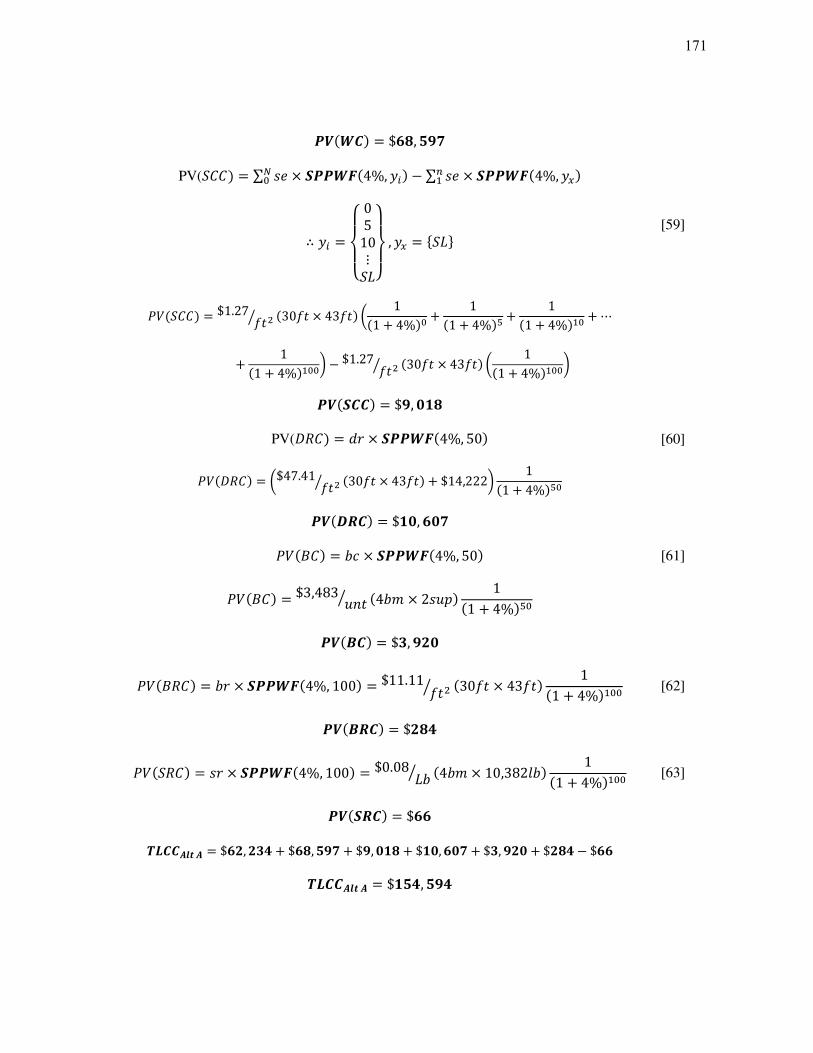
01�2�� = $E!, �oG

PV(�� = ∑ /, × H002K�4%, +\�N − ∑ /, × H002K�4%, +]�_

∴ +\ = abcbd 0510⋮��fbg

bh , +] = x��y [59]

�� = $1.27 789: �3078 × 4378� k 1�1 + 4%�N + 1�1 + 4%�= + 1�1 + 4%�_N +⋯+ 1�1 + 4%�_NNm − $1.27 789: �3078 × 4378� k 1�1 + 4%�_NNm

01�H�� = $o, p�!

PV(w�� = z. × H002K�4%, 50� [60]

��w�� = k$47.41 789: �3078 × 4378� + $14,222m 1�1 + 4%�=N

01�YR�� = $�p, EpG

�� = P# × H002K�4%, 50� [61]

�� = $3,483 {|8: �4P} × 2/{r� 1�1 + 4%�=N

01�Q�� = $ , oFp

�� = P. × H002K�4%, 100� = $11.11 789: �3078 × 4378� 1�1 + 4%�_NN [62]

01�QR�� = $F!�

�� = /. × H002K�4%, 100� = $0.08 �P: �4P} × 10,382~P� 1�1 + 4%�_NN [63]

01�HR�� = $EE

ST��UVWU = $EF, F � + $E!, �oG + $o, p�! + $�p, EpG + $ , oFp + $F!� − $EE

ST��UVWU = $��, �o�

171

A special discussion is needed for the FPG system since it is a new system included in this

study. As discussed in the literature review, there are two different configurations that can be

addressed using FPGs, the regular closed section and the inverted option with the bottom open for

inspection. The second option is a proprietary product, and its use involves an additional cost that

depends of the holder of the patent. These hidden costs are not available to the public, and

consequently it was decided to not include this option in this analysis. However, the closed section

is an open technology that can be used without restriction, and therefore it is used as the alternative

discussed in this report.

The FPG acts as a steel box section, and such sections are subjected to all the geometric

and proportion requirements given by the AASHTO LFRD specification, in particular section 6.11.

The requirement given by AASHTO LRFD Section 6.11.2.3 includes the maximum spacing

between parallel elements in order to use the distribution factors proposed by the code. This

requirement is based on the lateral distribution factors for steel box girders provided by Johnston

and Mattock (1967).

Using the section properties available and the AASHTO requirements it is mandatory to

use six (6) beams in the cross section of the bridge. The use of this additional beam (compared

with the total elements needed for a regular rolled I steel beam) increases the initial cost of this

alternative an amount that makes it not cost-effective. Nonetheless, a separate analysis was made

using a four (4) beam arrangement. A conservative assumption was made regarding the

distribution factors (considering the distribution factor as 1.00 for each beam), designing

accordingly the beam elements. This change increases the unit weight of each supporting element,

however, the final total weight is less than the six (6) beam alternative. Both LCCA are included

172

herein, proving that the six (6) beam configuration is not cost-effective while the four (4) beam

alternative is a competitive option. Further research is needed to explore the viability of 4 girders

and the applicability of AASHTO 6.11.2.3 for FPG girders.

Structural Steel Folded Plate Beams – 6 Beam Galvanized Configuration: Alternative A:

Bearing replacement, spot painting and sealing process. This option involves a deck

reconstruction (DRC) at 50 years, plus sealing and cleaning of the deck surface (SCC) every 5

years since the bridge construction, bearing replacements (BC) at 50 years, and washing of the

deck surface (WC) on a yearly basis, plus the initial cost (IC), the removal of the bridge cost (BRC)

and the salvage value represented by the benefit of selling the structural steel for recycling (SRC).

Structural steel beam elements with an exposed perimeter of 3.60ft. and a total weight of the steel

elements of 16,020 lb. Finally, a total price for the reinforcement steel of $8,375 which will be



�� = �� + �� + �� + ��w�� + �� + �� + �� [64]

�� = $EG, oF�

�� = "# × ZH02K�4%, 100+,-./�= $2.17 789: �3078 × 4378� �1 + 4%�_NN?@ABC − 14%�1 + 4%�_NN?@ABC

[65]

01�2�� = $E!, �oG

173

PV(�� = ∑ /, × H002K�4%, +\�N − ∑ /, × H002K�4%, +]�_

∴ +\ = abcbd 0510⋮��fbg

bh , +] = x��y [66]

�� = $1.27 789: �3078 × 4378� k 1�1 + 4%�N + 1�1 + 4%�= + 1�1 + 4%�_N +⋯+ 1�1 + 4%�_NNm − $1.27 789: �3078 × 4378� k 1�1 + 4%�_NNm

01�H�� = $o, p�!

PV(w�� = z. × H002K�4%, 50� [67]

��w�� = k$47.41 789: �3078 × 4378� + $8,375m 1�1 + 4%�=N

01�YR�� = $o, G!�

�� = P# × H002K�4%, 50� [68]

�� = $3,483 {|8: �6P} × 2/{r� �� + 4%�=N

01�Q�� = $�, !!�

�� = P. × H002K�4%, 100� = $11.11 789: �3078 × 4378� 1�1 + 4%�_NN [69]

01�QR�� = $F!�

�� = /. × H002K�4%, 100� = $0.08 �P: �6P} × 16,020~P� 1�1 + 4%�_NN [70]

01�HR�� = $��F

ST��UVWU = $EG, oF� + $E!, �oG + $o, p�! + $o, G!� + $F!� + $�, !!� − $��F

ST��UVWU = $�E�, F

174

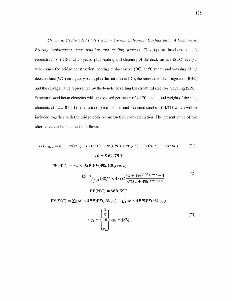
Structural Steel Folded Plate Beams – 4 Beam Galvanized Configuration: Alternative A:

Bearing replacement, spot painting and sealing process. This option involves a deck

reconstruction (DRC) at 50 years, plus sealing and cleaning of the deck surface (SCC) every 5

years since the bridge construction, bearing replacements (BC) at 50 years, and washing of the

deck surface (WC) on a yearly basis, plus the initial cost (IC), the removal of the bridge cost (BRC)

and the salvage value represented by the benefit of selling the structural steel for recycling (SRC).

Structural steel beam elements with an exposed perimeter of 4.17ft. and a total weight of the steel

elements of 12,240 lb. Finally, a total price for the reinforcement steel of $14,222 which will be



�� = �� + �� + �� + ��w�� + �� + �� + �� [71]

�� = $EF, Gop

�� = "# × ZH02K�4%, 100+,-./�= $2.17 789: �3078 × 4378� �1 + 4%�_NN?@ABC − 14%�1 + 4%�_NN?@ABC

[72]

01�2�� = $E!, �oG

PV(�� = ∑ /, × H002K�4%, +\�N − ∑ /, × H002K�4%, +]�_

∴ +\ = abcbd 0510⋮��fbg

bh , +] = x��y [73]

175

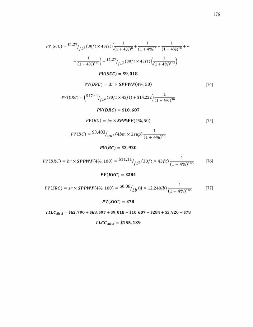
�� = $1.27 789: �3078 × 4378� k 1�1 + 4%�N + 1�1 + 4%�= + 1�1 + 4%�_N +⋯+ 1�1 + 4%�_NNm − $1.27 789: �3078 × 4378� k 1�1 + 4%�_NNm

01�H�� = $o, p�!

PV(w�� = z. × H002K�4%, 50� [74]

��w�� = k$47.41 789: �3078 × 4378� + $14,222m 1�1 + 4%�=N

01�YR�� = $�p, EpG

�� = P# × H002K�4%, 50� [75]

�� = $3,483 {|8: �4P} × 2/{r� 1�1 + 4%�=N

01�Q�� = $ , oFp

�� = P. × H002K�4%, 100� = $11.11 789: �3078 × 4378� 1�1 + 4%�_NN [76]

01�QR�� = $F!�

�� = /. × H002K�4%, 100� = $0.08 �P: �4 × 12,240~P� 1�1 + 4%�_NN [77]

01�HR�� = $G!

ST��UVWU = $EF, Gop + $E!, �oG + $o, p�! + $�p, EpG + $F!� + $ , oFp − $G!

ST��UVWU = $��, � o

176

177

F. STOCHASTIC DOMINANCE RESULTS FOR

SUPERSTRUCTURE SELECTION

This appendix present the summary of the results obtained from the Monte Carlo

simulation and used for the superstructure selection using stochastic dominance. A

summary table is used for superstructure selection for each case. Each table shows the

stochastic matrix selection, in this, each cell shows a set of logical values composed of

4 figures, namely, first, second, almost first and almost second stochastic dominance.

As a convention, 0 indicates not dominance of the option shown in the row to the

option contrasted in the column, while 1 means dominance in any degree of the row

alternative to the column option. For example, if the logical output is “0-0-1-1”, it

means that the option shown in the row almost dominates in first degree the option

presented in the column, Column �almost1 Row. In other words, the option in the

column is most cost-effective than the option shown in the row and is more preferable

for that specific span length. The final objective is to find a column that is dominated

by every row in the stochastic dominance matrix.

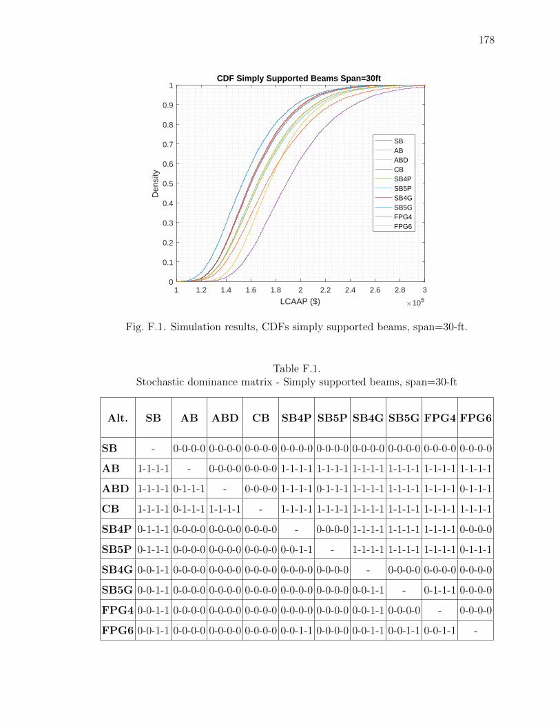
178

1 1.2 1.4 1.6 1.8 2 2.2 2.4 2.6 2.8 3

LCAAP ($) 105

0

0.1

0.2

0.3

0.4

0.5

0.6

0.7

0.8

0.9

1

Den

sity


SBABABDCBSB4PSB5PSB4GSB5GFPG4FPG6

Fig. F.1. Simulation results, CDFs simply supported beams, span=30-ft.

Table F.1.Stochastic dominance matrix - Simply supported beams, span=30-ft

Alt. SB AB ABD CB SB4P SB5P SB4G SB5G FPG4 FPG6

SB - 0-0-0-0 0-0-0-0 0-0-0-0 0-0-0-0 0-0-0-0 0-0-0-0 0-0-0-0 0-0-0-0 0-0-0-0

AB 1-1-1-1 - 0-0-0-0 0-0-0-0 1-1-1-1 1-1-1-1 1-1-1-1 1-1-1-1 1-1-1-1 1-1-1-1

ABD 1-1-1-1 0-1-1-1 - 0-0-0-0 1-1-1-1 0-1-1-1 1-1-1-1 1-1-1-1 1-1-1-1 0-1-1-1

CB 1-1-1-1 0-1-1-1 1-1-1-1 - 1-1-1-1 1-1-1-1 1-1-1-1 1-1-1-1 1-1-1-1 1-1-1-1

SB4P 0-1-1-1 0-0-0-0 0-0-0-0 0-0-0-0 - 0-0-0-0 1-1-1-1 1-1-1-1 1-1-1-1 0-0-0-0

SB5P 0-1-1-1 0-0-0-0 0-0-0-0 0-0-0-0 0-0-1-1 - 1-1-1-1 1-1-1-1 1-1-1-1 0-1-1-1

SB4G 0-0-1-1 0-0-0-0 0-0-0-0 0-0-0-0 0-0-0-0 0-0-0-0 - 0-0-0-0 0-0-0-0 0-0-0-0

SB5G 0-0-1-1 0-0-0-0 0-0-0-0 0-0-0-0 0-0-0-0 0-0-0-0 0-0-1-1 - 0-1-1-1 0-0-0-0

FPG4 0-0-1-1 0-0-0-0 0-0-0-0 0-0-0-0 0-0-0-0 0-0-0-0 0-0-1-1 0-0-0-0 - 0-0-0-0

FPG6 0-0-1-1 0-0-0-0 0-0-0-0 0-0-0-0 0-0-1-1 0-0-0-0 0-0-1-1 0-0-1-1 0-0-1-1 -

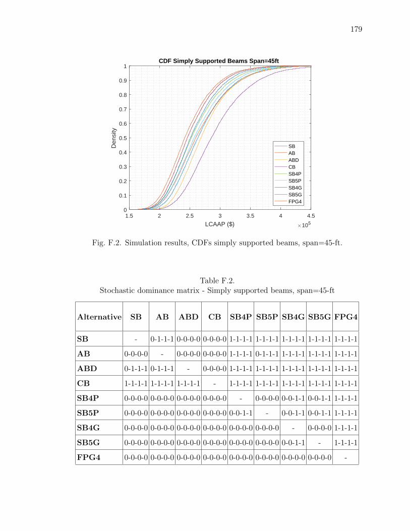
179

1.5 2 2.5 3 3.5 4 4.5

LCAAP ($) 105

0

0.1

0.2

0.3

0.4

0.5

0.6

0.7

0.8

0.9

1

Den

sity


SBABABDCBSB4PSB5PSB4GSB5GFPG4



Alternative SB AB ABD CB SB4P SB5P SB4G SB5G FPG4

SB - 0-1-1-1 0-0-0-0 0-0-0-0 1-1-1-1 1-1-1-1 1-1-1-1 1-1-1-1 1-1-1-1

AB 0-0-0-0 - 0-0-0-0 0-0-0-0 1-1-1-1 0-1-1-1 1-1-1-1 1-1-1-1 1-1-1-1

ABD 0-1-1-1 0-1-1-1 - 0-0-0-0 1-1-1-1 1-1-1-1 1-1-1-1 1-1-1-1 1-1-1-1

CB 1-1-1-1 1-1-1-1 1-1-1-1 - 1-1-1-1 1-1-1-1 1-1-1-1 1-1-1-1 1-1-1-1

SB4P 0-0-0-0 0-0-0-0 0-0-0-0 0-0-0-0 - 0-0-0-0 0-0-1-1 0-0-1-1 1-1-1-1

SB5P 0-0-0-0 0-0-0-0 0-0-0-0 0-0-0-0 0-0-1-1 - 0-0-1-1 0-0-1-1 1-1-1-1

SB4G 0-0-0-0 0-0-0-0 0-0-0-0 0-0-0-0 0-0-0-0 0-0-0-0 - 0-0-0-0 1-1-1-1

SB5G 0-0-0-0 0-0-0-0 0-0-0-0 0-0-0-0 0-0-0-0 0-0-0-0 0-0-1-1 - 1-1-1-1

FPG4 0-0-0-0 0-0-0-0 0-0-0-0 0-0-0-0 0-0-0-0 0-0-0-0 0-0-0-0 0-0-0-0 -

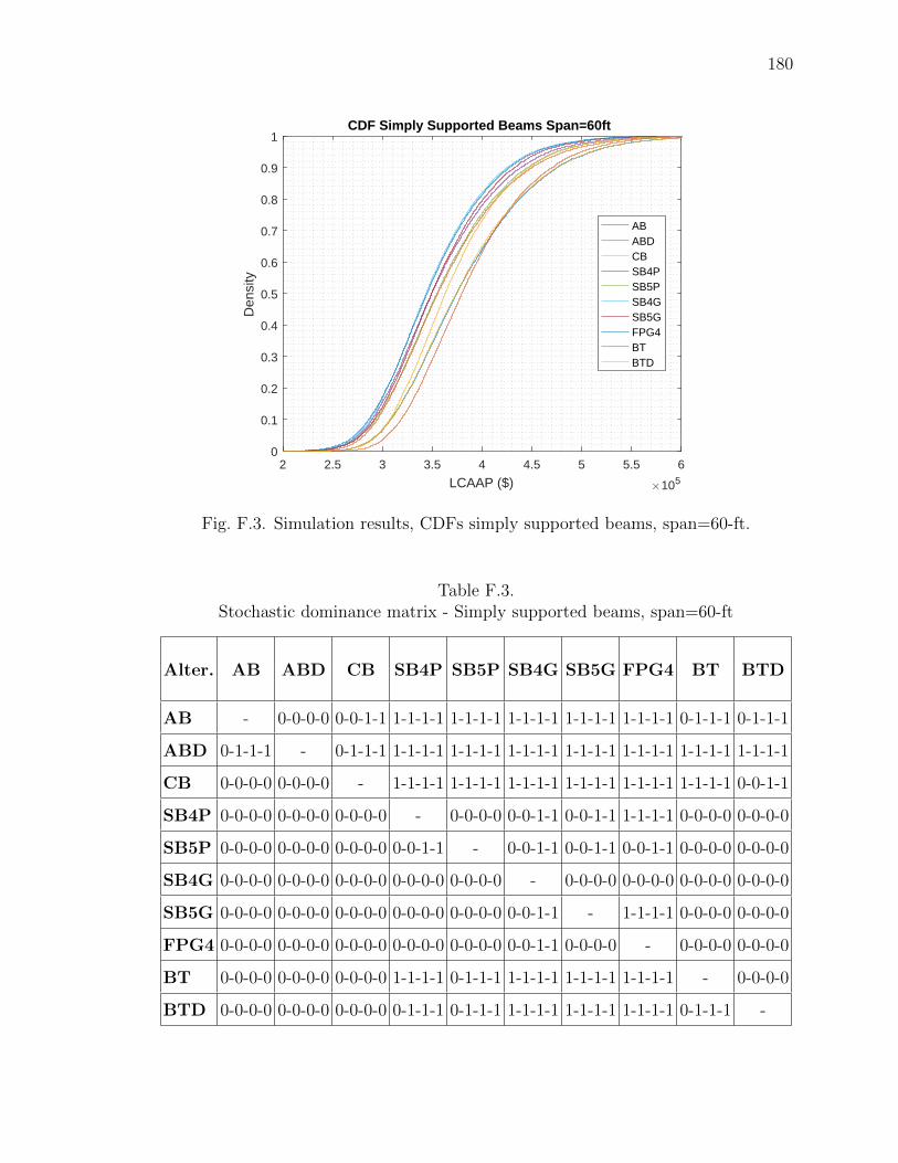
180

2 2.5 3 3.5 4 4.5 5 5.5 6

LCAAP ($) 105

0

0.1

0.2

0.3

0.4

0.5

0.6

0.7

0.8

0.9

1

Den

sity


ABABDCBSB4PSB5PSB4GSB5GFPG4BTBTD



Alter. AB ABD CB SB4P SB5P SB4G SB5G FPG4 BT BTD

AB - 0-0-0-0 0-0-1-1 1-1-1-1 1-1-1-1 1-1-1-1 1-1-1-1 1-1-1-1 0-1-1-1 0-1-1-1

ABD 0-1-1-1 - 0-1-1-1 1-1-1-1 1-1-1-1 1-1-1-1 1-1-1-1 1-1-1-1 1-1-1-1 1-1-1-1

CB 0-0-0-0 0-0-0-0 - 1-1-1-1 1-1-1-1 1-1-1-1 1-1-1-1 1-1-1-1 1-1-1-1 0-0-1-1

SB4P 0-0-0-0 0-0-0-0 0-0-0-0 - 0-0-0-0 0-0-1-1 0-0-1-1 1-1-1-1 0-0-0-0 0-0-0-0

SB5P 0-0-0-0 0-0-0-0 0-0-0-0 0-0-1-1 - 0-0-1-1 0-0-1-1 0-0-1-1 0-0-0-0 0-0-0-0

SB4G 0-0-0-0 0-0-0-0 0-0-0-0 0-0-0-0 0-0-0-0 - 0-0-0-0 0-0-0-0 0-0-0-0 0-0-0-0

SB5G 0-0-0-0 0-0-0-0 0-0-0-0 0-0-0-0 0-0-0-0 0-0-1-1 - 1-1-1-1 0-0-0-0 0-0-0-0

FPG4 0-0-0-0 0-0-0-0 0-0-0-0 0-0-0-0 0-0-0-0 0-0-1-1 0-0-0-0 - 0-0-0-0 0-0-0-0

BT 0-0-0-0 0-0-0-0 0-0-0-0 1-1-1-1 0-1-1-1 1-1-1-1 1-1-1-1 1-1-1-1 - 0-0-0-0

BTD 0-0-0-0 0-0-0-0 0-0-0-0 0-1-1-1 0-1-1-1 1-1-1-1 1-1-1-1 1-1-1-1 0-1-1-1 -

181

3 3.5 4 4.5 5 5.5 6 6.5 7 7.5 8

LCAAP ($) 105

0

0.1

0.2

0.3

0.4

0.5

0.6

0.7

0.8

0.9

1

Den

sity


ABABDSB4PSB5PSB4GSB5GBTBTD



Alternative AB ABD SB4P SB5P SB4G SB5G BT BTD

AB - 0-0-0-0 0-0-0-0 0-0-0-0 0-0-0-0 0-0-0-0 0-1-1-1 0-0-1-1

ABD 0-1-1-1 - 0-1-1-1 0-0-0-1 1-1-1-1 0-0-0-0 1-1-1-1 1-1-1-1

SB4P 0-0-1-1 0-0-0-0 - 0-0-0-0 0-0-1-1 0-0-0-0 0-0-1-1 0-0-1-1

SB5P 0-0-1-1 0-0-1-1 0-1-1-1 - 0-0-1-1 0-0-1-1 0-0-1-1 0-0-1-1

SB4G 0-0-1-1 0-0-0-0 0-0-0-0 0-0-0-0 - 0-0-0-0 0-0-1-1 0-0-1-1

SB5G 0-0-1-1 0-0-1-1 0-1-1-1 0-0-0-0 0-0-1-1 - 0-0-1-1 0-0-1-1

BT 0-0-0-0 0-0-0-0 0-0-0-0 0-0-0-0 0-0-0-0 0-0-0-0 - 0-0-0-0

BTD 0-0-0-0 0-0-0-0 0-0-0-0 0-0-0-0 0-0-0-0 0-0-0-0 0-1-1-1 -

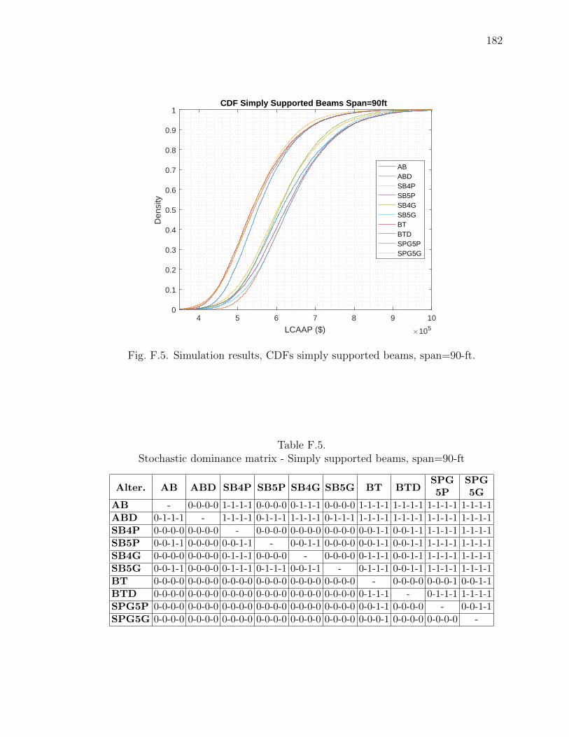
182

4 5 6 7 8 9 10

LCAAP ($) 105

0

0.1

0.2

0.3

0.4

0.5

0.6

0.7

0.8

0.9

1

Den

sity


ABABDSB4PSB5PSB4GSB5GBTBTDSPG5PSPG5G



Alter. AB ABD SB4P SB5P SB4G SB5G BT BTDSPG SPG5P 5G

AB - 0-0-0-0 1-1-1-1 0-0-0-0 0-1-1-1 0-0-0-0 1-1-1-1 1-1-1-1 1-1-1-1 1-1-1-1ABD 0-1-1-1 - 1-1-1-1 0-1-1-1 1-1-1-1 0-1-1-1 1-1-1-1 1-1-1-1 1-1-1-1 1-1-1-1SB4P 0-0-0-0 0-0-0-0 - 0-0-0-0 0-0-0-0 0-0-0-0 0-0-1-1 0-0-1-1 1-1-1-1 1-1-1-1SB5P 0-0-1-1 0-0-0-0 0-0-1-1 - 0-0-1-1 0-0-0-0 0-0-1-1 0-0-1-1 1-1-1-1 1-1-1-1SB4G 0-0-0-0 0-0-0-0 0-1-1-1 0-0-0-0 - 0-0-0-0 0-1-1-1 0-0-1-1 1-1-1-1 1-1-1-1SB5G 0-0-1-1 0-0-0-0 0-1-1-1 0-1-1-1 0-0-1-1 - 0-1-1-1 0-0-1-1 1-1-1-1 1-1-1-1BT 0-0-0-0 0-0-0-0 0-0-0-0 0-0-0-0 0-0-0-0 0-0-0-0 - 0-0-0-0 0-0-0-1 0-0-1-1BTD 0-0-0-0 0-0-0-0 0-0-0-0 0-0-0-0 0-0-0-0 0-0-0-0 0-1-1-1 - 0-1-1-1 1-1-1-1SPG5P 0-0-0-0 0-0-0-0 0-0-0-0 0-0-0-0 0-0-0-0 0-0-0-0 0-0-1-1 0-0-0-0 - 0-0-1-1SPG5G 0-0-0-0 0-0-0-0 0-0-0-0 0-0-0-0 0-0-0-0 0-0-0-0 0-0-0-1 0-0-0-0 0-0-0-0 -

183

4 5 6 7 8 9 10 11

LCAAP ($) 105

0

0.1

0.2

0.3

0.4

0.5

0.6

0.7

0.8

0.9

1

Den

sity


BTBTDSPG5PSPG5G



Alternative BT BTD SPG5P SPG5G

BT - 0-0-0-0 0-0-0-0 0-0-0-0

BTD 0-1-1-1 - 0-1-1-1 1-1-1-1

SPG5P 0-0-1-1 0-0-0-0 - 0-0-1-1

SPG5G 0-0-1-1 0-0-0-0 0-0-0-0 -

184

0.4 0.6 0.8 1 1.2 1.4 1.6 1.8

LCAAP ($) 106

0

0.1

0.2

0.3

0.4

0.5

0.6

0.7

0.8

0.9

1

Den

sity


BTBTDSPG5PSPG5G




BT - 0-0-0-0 0-0-0-0 0-0-0-0

BTD 0-1-1-1 - 0-0-0-0 0-0-0-0

SPG5P 0-0-1-1 0-0-1-1 - 0-0-0-0

SPG5G 1-1-1-1 0-0-1-1 0-1-1-1 -

185

2 3 4 5 6 7 8 9 10

LCAAP ($) 105

0

0.1

0.2

0.3

0.4

0.5

0.6

0.7

0.8

0.9

1

Den

sity


SBCB

Fig. F.8. Simulation results, CDFs continuous beams, span=30-ft.

Table F.8.Stochastic dominance matrix - Continuous beams, span=30-ft

Alternative SB CB

SB - 0-0-0-0

CB 1-1-1-1 -

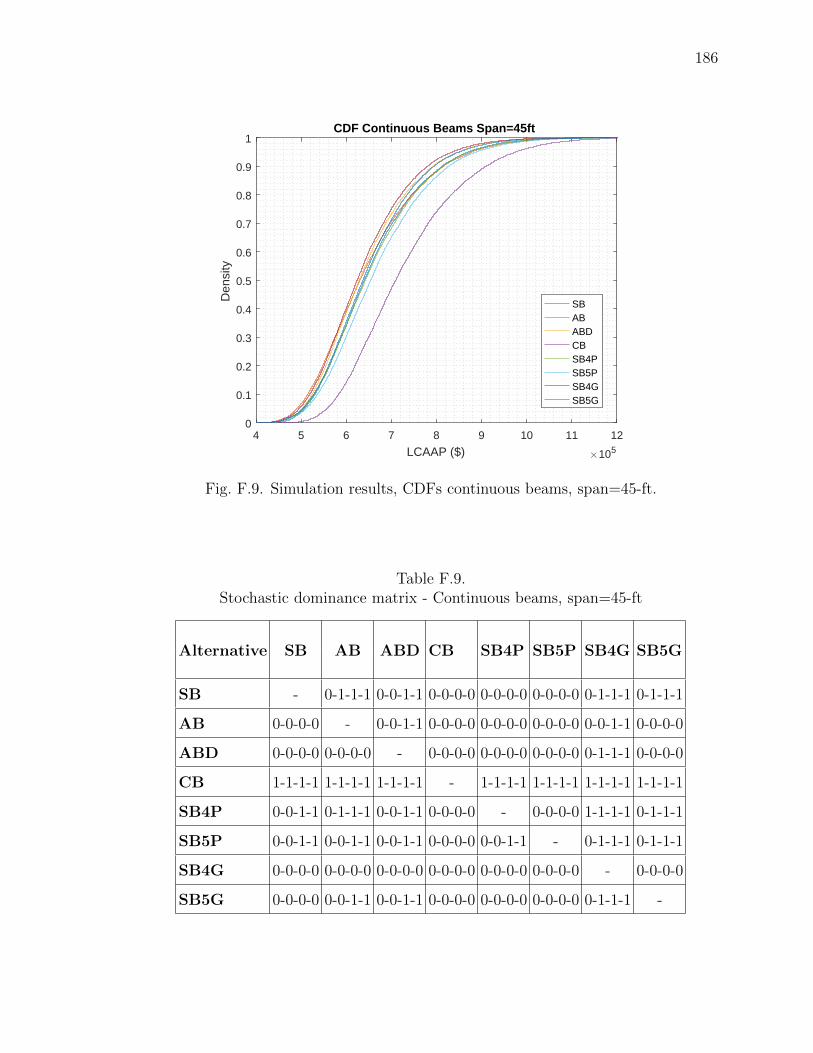
186

4 5 6 7 8 9 10 11 12

LCAAP ($) 105

0

0.1

0.2

0.3

0.4

0.5

0.6

0.7

0.8

0.9

1

Den

sity


SBABABDCBSB4PSB5PSB4GSB5G



Alternative SB AB ABD CB SB4P SB5P SB4G SB5G

SB - 0-1-1-1 0-0-1-1 0-0-0-0 0-0-0-0 0-0-0-0 0-1-1-1 0-1-1-1

AB 0-0-0-0 - 0-0-1-1 0-0-0-0 0-0-0-0 0-0-0-0 0-0-1-1 0-0-0-0

ABD 0-0-0-0 0-0-0-0 - 0-0-0-0 0-0-0-0 0-0-0-0 0-1-1-1 0-0-0-0

CB 1-1-1-1 1-1-1-1 1-1-1-1 - 1-1-1-1 1-1-1-1 1-1-1-1 1-1-1-1

SB4P 0-0-1-1 0-1-1-1 0-0-1-1 0-0-0-0 - 0-0-0-0 1-1-1-1 0-1-1-1

SB5P 0-0-1-1 0-0-1-1 0-0-1-1 0-0-0-0 0-0-1-1 - 0-1-1-1 0-1-1-1

SB4G 0-0-0-0 0-0-0-0 0-0-0-0 0-0-0-0 0-0-0-0 0-0-0-0 - 0-0-0-0

SB5G 0-0-0-0 0-0-1-1 0-0-1-1 0-0-0-0 0-0-0-0 0-0-0-0 0-1-1-1 -

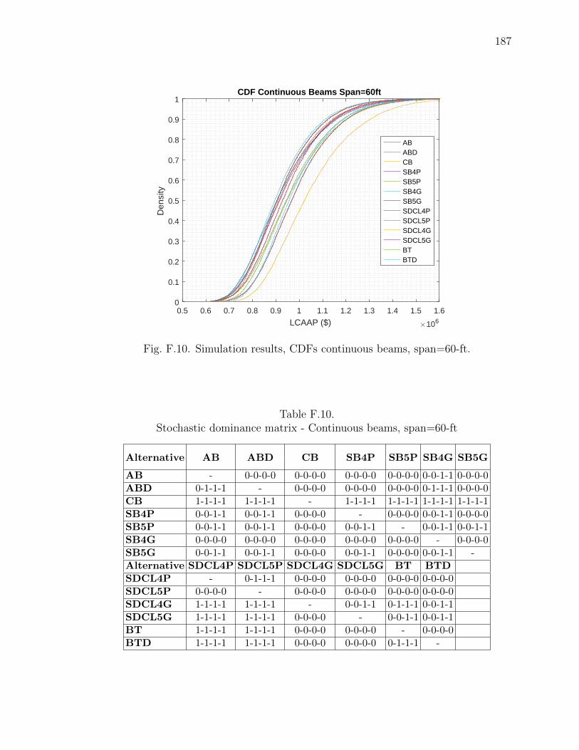
187

0.5 0.6 0.7 0.8 0.9 1 1.1 1.2 1.3 1.4 1.5 1.6

LCAAP ($) 106

0

0.1

0.2

0.3

0.4

0.5

0.6

0.7

0.8

0.9

1

Den

sity


ABABDCBSB4PSB5PSB4GSB5GSDCL4PSDCL5PSDCL4GSDCL5GBTBTD



Alternative AB ABD CB SB4P SB5P SB4G SB5G

AB - 0-0-0-0 0-0-0-0 0-0-0-0 0-0-0-0 0-0-1-1 0-0-0-0ABD 0-1-1-1 - 0-0-0-0 0-0-0-0 0-0-0-0 0-1-1-1 0-0-0-0CB 1-1-1-1 1-1-1-1 - 1-1-1-1 1-1-1-1 1-1-1-1 1-1-1-1SB4P 0-0-1-1 0-0-1-1 0-0-0-0 - 0-0-0-0 0-0-1-1 0-0-0-0SB5P 0-0-1-1 0-0-1-1 0-0-0-0 0-0-1-1 - 0-0-1-1 0-0-1-1SB4G 0-0-0-0 0-0-0-0 0-0-0-0 0-0-0-0 0-0-0-0 - 0-0-0-0SB5G 0-0-1-1 0-0-1-1 0-0-0-0 0-0-1-1 0-0-0-0 0-0-1-1 -Alternative SDCL4P SDCL5P SDCL4G SDCL5G BT BTDSDCL4P - 0-1-1-1 0-0-0-0 0-0-0-0 0-0-0-0 0-0-0-0SDCL5P 0-0-0-0 - 0-0-0-0 0-0-0-0 0-0-0-0 0-0-0-0SDCL4G 1-1-1-1 1-1-1-1 - 0-0-1-1 0-1-1-1 0-0-1-1SDCL5G 1-1-1-1 1-1-1-1 0-0-0-0 - 0-0-1-1 0-0-1-1BT 1-1-1-1 1-1-1-1 0-0-0-0 0-0-0-0 - 0-0-0-0BTD 1-1-1-1 1-1-1-1 0-0-0-0 0-0-0-0 0-1-1-1 -

188

0.8 1 1.2 1.4 1.6 1.8 2

LCAAP ($) 106

0

0.1

0.2

0.3

0.4

0.5

0.6

0.7

0.8

0.9

1

Den

sity


ABABDSDCL4PSDCL5PSDCL4GSDCL5GBTBTD



Alternative AB ABD SDCL4P SDCL5P SDCL4G SDCL5G BT BTD

AB - 0-0-0-0 0-0-0-0 0-0-0-0 0-0-0-0 0-0-0-0 0-1-1-1 0-0-1-1ABD 0-1-1-1 - 0-1-1-1 0-0-0-0 0-0-0-0 0-0-0-0 0-1-1-1 1-1-1-1SDCL4P 0-0-1-1 0-0-0-0 - 0-0-0-0 0-0-0-0 0-0-0-0 0-0-1-1 0-0-1-1SDCL5P 0-0-1-1 0-0-1-1 0-0-1-1 - 0-0-0-0 0-0-0-0 0-0-1-1 0-0-1-1SDCL4G 0-1-1-1 0-0-1-1 1-1-1-1 1-1-1-1 - 0-0-0-0 1-1-1-1 1-1-1-1SDCL5G 0-0-1-1 0-0-1-1 1-1-1-1 1-1-1-1 0-0-1-1 - 1-1-1-1 1-1-1-1BT 0-0-0-0 0-0-0-0 0-0-0-0 0-0-0-0 0-0-0-0 0-0-0-0 - 0-0-0-0BTD 0-0-0-0 0-0-0-0 0-0-0-0 0-0-0-0 0-0-0-0 0-0-0-0 0-1-1-1 -

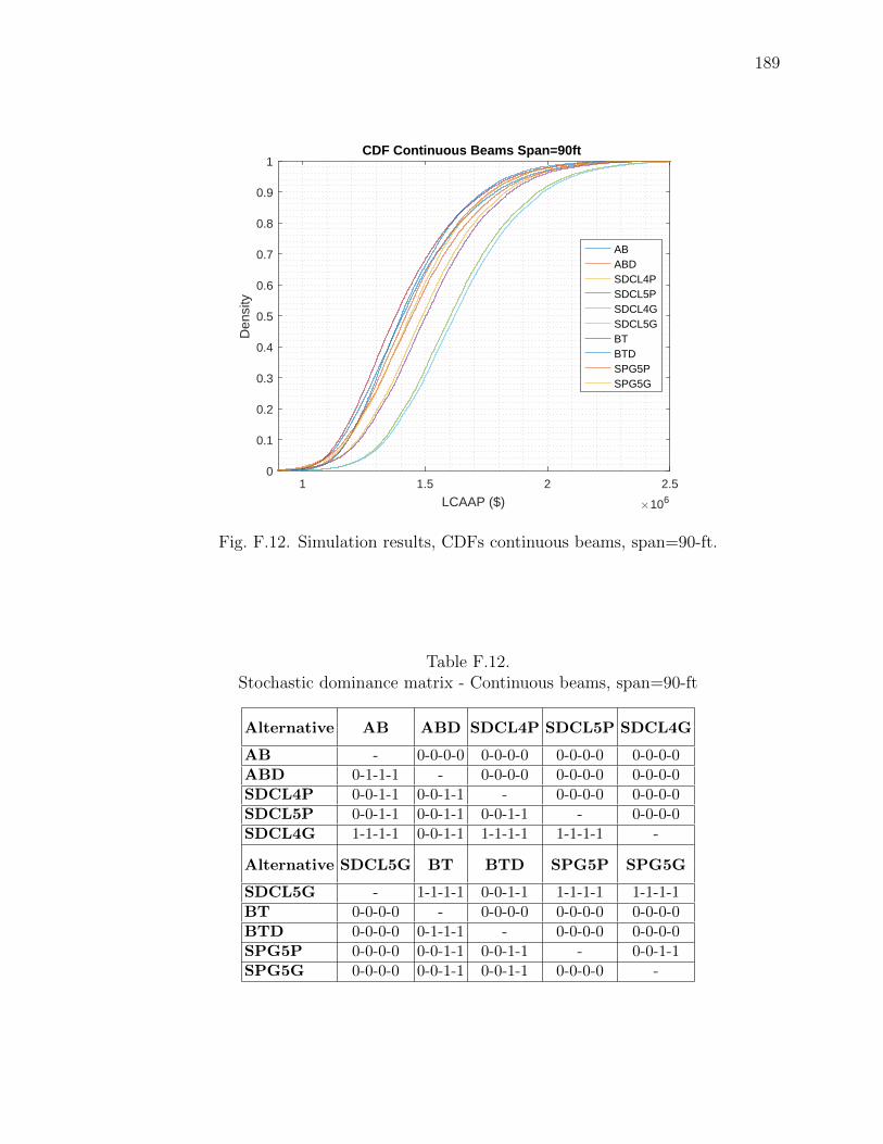
189

1 1.5 2 2.5

LCAAP ($) 106

0

0.1

0.2

0.3

0.4

0.5

0.6

0.7

0.8

0.9

1

Den

sity


ABABDSDCL4PSDCL5PSDCL4GSDCL5GBTBTDSPG5PSPG5G



Alternative AB ABD SDCL4P SDCL5P SDCL4G

AB - 0-0-0-0 0-0-0-0 0-0-0-0 0-0-0-0ABD 0-1-1-1 - 0-0-0-0 0-0-0-0 0-0-0-0SDCL4P 0-0-1-1 0-0-1-1 - 0-0-0-0 0-0-0-0SDCL5P 0-0-1-1 0-0-1-1 0-0-1-1 - 0-0-0-0SDCL4G 1-1-1-1 0-0-1-1 1-1-1-1 1-1-1-1 -

Alternative SDCL5G BT BTD SPG5P SPG5G

SDCL5G - 1-1-1-1 0-0-1-1 1-1-1-1 1-1-1-1BT 0-0-0-0 - 0-0-0-0 0-0-0-0 0-0-0-0BTD 0-0-0-0 0-1-1-1 - 0-0-0-0 0-0-0-0SPG5P 0-0-0-0 0-0-1-1 0-0-1-1 - 0-0-1-1SPG5G 0-0-0-0 0-0-1-1 0-0-1-1 0-0-0-0 -

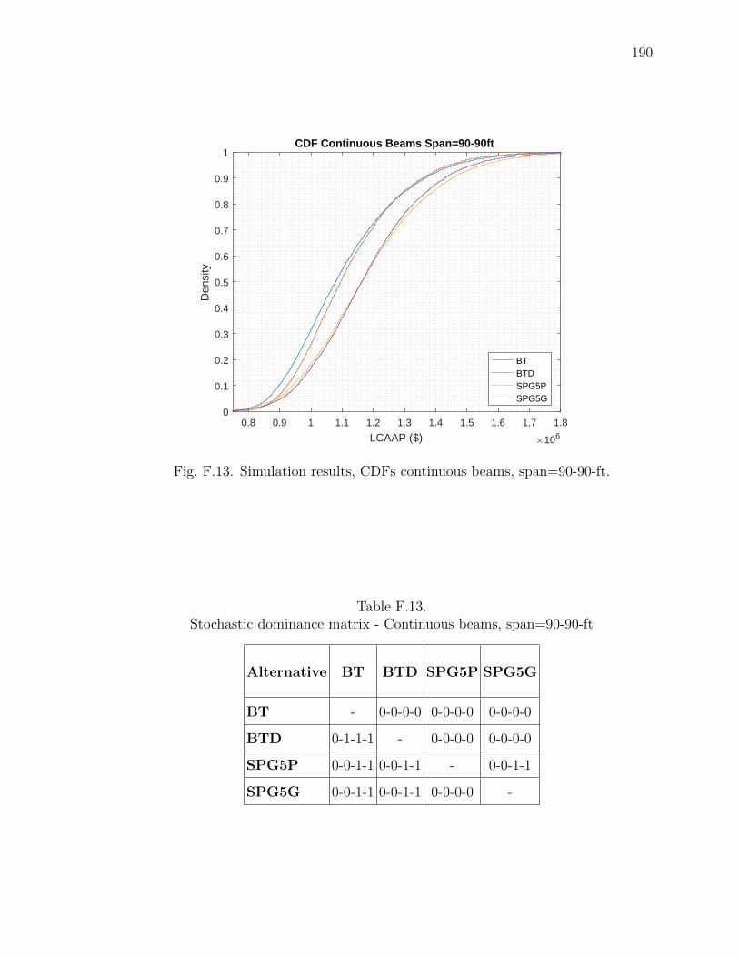
190

0.8 0.9 1 1.1 1.2 1.3 1.4 1.5 1.6 1.7 1.8

LCAAP ($) 106

0

0.1

0.2

0.3

0.4

0.5

0.6

0.7

0.8

0.9

1

Den

sity

CDF Continuous Beams Span=90-90ft

BTBTDSPG5PSPG5G

Fig. F.13. Simulation results, CDFs continuous beams, span=90-90-ft.

Table F.13.Stochastic dominance matrix - Continuous beams, span=90-90-ft


BT - 0-0-0-0 0-0-0-0 0-0-0-0

BTD 0-1-1-1 - 0-0-0-0 0-0-0-0

SPG5P 0-0-1-1 0-0-1-1 - 0-0-1-1

SPG5G 0-0-1-1 0-0-1-1 0-0-0-0 -

191

1 1.2 1.4 1.6 1.8 2 2.2

LCAAP ($) 106

0

0.1

0.2

0.3

0.4

0.5

0.6

0.7

0.8

0.9

1

Den

sity


BTBTDSPG5PSPG5G




BT - 0-0-0-0 0-0-0-0 0-0-0-0

BTD 0-1-1-1 - 0-0-0-0 0-0-1-1

SPG5P 0-0-1-1 0-0-1-1 - 0-0-1-1

SPG5G 0-0-1-1 0-0-1-1 0-0-0-0 -

192

1.2 1.4 1.6 1.8 2 2.2 2.4 2.6 2.8

LCAAP ($) 106

0

0.1

0.2

0.3

0.4

0.5

0.6

0.7

0.8

0.9

1

Den

sity


BTBTDSPG5PSPG5G




BT - 0-0-0-0 0-0-0-0 0-0-0-0

BTD 0-1-1-1 - 0-0-0-0 0-0-0-0

SPG5P 0-0-1-1 0-0-1-1 - 0-0-0-0

SPG5G 0-0-1-1 0-0-1-1 0-1-1-1 -

VITA

193

VITA

Stefan L. Leiva Maldonado was born in Bogota, Colombia on May 12, 1988. He ob-

tained his undergraduate degree in Civil Engineering in March 2011 from Universidad

Distrital Francisco Jos de Caldas, Bogot, Colombia. In August 2011 Stefan joined

the Civil Engineering Masters program from Universidad Nacional, Bogot, Colom-

bia, and obtained his Masters degree in 2015. During his studies Stefan has been

working actively in the Colombian industry as structural designer. His experience

in structural design in a wide range of projects and specialized in steel structures

gave him the opportunity to join projects with huge impact in Colombian infrastruc-

ture as “El Quimbo dam”, “Sogamoso hydroelectric Project”, “CERROMATOSO

S.A Mine workshop replacement”, and many others. In 2013 Stefan was awarded

with the Fulbright-Colciencias fellowship to continue his studies in one of the most

important universities in United States. Stefan joined Purdue University as PhD stu-

dent in spring 2014 and worked in a project founded by the Indiana Department of

Transportation (INDOT) focused on Life cycle cost analysis (LCCA) of concrete and

steel bridges for short spans. He received his Ph.D. in civil engineering from Purdue

University in August 2019.