Supercritical Dirac resonance parameters from extrapolated analytic continuation methods

arX

iv:0

705.

4318

v2 [

phys

ics.

atom

-ph]

5 J

ul 2

007

Supercritical Dirac resonance parameters from extrapolated

analytic continuation methods

Edward Ackad and Marko Horbatsch

Department of Physics and Astronomy, York University,

4700 Keele St, Toronto, Ontario, Canada M3J 1P3

Abstract

The analytic continuation methods of complex scaling (CS), smooth exterior scaling (SES), and

complex absorbing potential (CAP) are investigated for the supercritical quasimolecular ground

state in the U92+-Cf98+ system at an internuclear separation of R = 20 fm. Pade approximants

to the complex-energy trajectories are used to perform an extrapolation of the resonance energies,

which, thus, become independent of the respective stabilization parameter. Within the monopole

approximation to the two-center potential is demonstrated that the extrapolated results from SES

and CAP are consistent to a high degree of accuracy. Extrapolated CAP calculations are extended

to include dipole and quadrupole terms of the potential for a large range of internuclear separations

R. These terms cause a broadening of the widths at the 0/00 level when the nuclei are almost in

contact, and at the % level for R values where the 1Sσ state enters the negative continuum.

1

I. INTRODUCTION

The ability to produce super-strong electric fields in experiments, either by super-intense

lasers or in collisions with highly ionized heavy atoms, opens the possibility to study nonlin-

ear phenomena. It allows for detailed testing of the interface of relativistic quantum mechan-

ics and quantum electrodynamics by probing electron dynamics at an energy scale where

phenomena such as electron-positron pair creation may be detected against the background

of more conventional atomic physics processes such as ionization and positron production

by time-dependent fields [1].

An electron in a Coulomb potential represents a problem that has been studied in both

relativistic and non-relativistic physics. As the potential depth increases with nuclear charge

Z, the ground state’s energy decreases as Z2. Since the spectrum of the Dirac equation for

a Coulomb potential is not bounded from below (due to the negative-energy continuum

E < −mec2), a potential of sufficient strength can yield resonance states when the ground-

state energy E1S < −mec2. This causes the QED vacuum to become unstable and decay

by pair-creation to a charged vacuum state [2]. The potential is called super-critical in this

case.

For a Coulomb potential, a single nucleus would need to be much more massive than any

observed element (Z ∼> 169 for finite-size nuclei), but when two large nuclei get close enough,

the combined two-center potential can become supercritical [2, 3]. As the two nuclei get

closer the energy of the quasi-molecular ground state (1Sσ) decreases and so the resonance

energy is embedded deeper into the negative-energy continuum of the Dirac spectrum. These

negative-energy electron states can be reinterpreted using CPT symmetry as positron states

of positive energy. Therefore, by studying these supercritical resonances, the dynamics of

2

systems at the energy scale of particle creation can be explored.

It is possible to build a matrix representation of the hermitian two-center Hamiltonian for

a supercritical potential in order to measure the resonance parameters from the Lorentzian

distributions in the energy spectrum or from the density of states [4]. More accurate results

were obtained from analytic continuation methods which yield discrete resonance states with

the following properties: (i) bounded, square-integrable eigenfunctions,i.e., elements of the

Hilbert space of the original Hamiltonian; (ii) complex eigenenergies, ER, whose real and

imaginary parts agree with the center and width of the Lorentzian shape in the spectrum

of the original Hamiltonian. Note that the imaginary part is positive, i.e., ER = Eres + iΓ/2

for Dirac states with Eres < −mec2 [4].

Analytic continuation makes use of some parameter ζ to turn the original Hamiltonian

into a non-hermitian operator. This raises two problems: (i) one has to optimize ζ to find

the best approximation to the complex resonance eigenenergy; (ii) one worries about the

effect of the unphysical ζ parameter on the final result. The optimization in step (i) is

performed by stabilizing some measure that depends on the eigenenergy as a function of ζ

(such as, e.g., the magnitude |ER(ζ)|).

Recent work for the method of adding a complex absorbing potential (CAP) has demon-

strated how to obtain more accurate results by extrapolating the complex ER(ζ)-trajectory

to ζ = 0 [5]. The present work extends this idea to the relativistic Dirac equation using the

complementary methods of smooth exterior scaling (SES) and CAP. The stability and pa-

rameter independence of the results is demonstrated. The extrapolation technique enables

us to perform an extension of the calculations beyond the monopole approximation to the

two-center potential. Results are given for the three coupled channels, κ = −1, 1,−2, for

a large range of internuclear separation, i.e., the resonance width broadening due to dipole

3

and quadrupole interactions is calculated.

II. THEORY

A. Complex absorbing potential method

The method of adding a complex absorbing potential (CAP) to the Hamiltonian has

been used extensively in atomic and molecular physics [6, 7, 8, 9], and was put on firm

mathematical grounds by Riss and Meyer [10]. It was recently extended to the relativistic

Dirac equation for Stark resonances [11], and for supercritical resonances [4]. It works by

extending the physical Hamiltonian by an imaginary potential which makes the Hamiltonian

non-hermitian. In the case of the Dirac Hamiltonian a CAP is added as a scalar giving,

HCAP = H − iηβW (r), (1)

where η is a small non-negative parameter determining the strength of the CAP and β is

the standard Dirac matrix [3]. The function W (r) determines the shape of the potential

and is tailored for the specific problem. Currently, the most common use of a CAP is as

a stabilization method: one solves the system on an equally spaced mesh of values of η

and takes the minimum of∣

∣

∣η dER

dη

∣

∣

∣

η=ηopt

as the closest approximation to the true resonance

parameters [10].

In the present work we chose

W (r) = Θ(r − rc) (r − rc)2 (2)

for the CAP, where Θ is the Heaviside function. The CAP parameter rc allows for the

turn-on of the potential outside of the “bound” part of the wavefunction [12].

4

B. Smooth exterior scaling method

Smooth exterior scaling (SES) is an extension of the complex scaling (CS) method whose

mathematical justification was developed, e.g., by W.P. Reinhardt [13], and Moiseyev [14].

CS introduces an analytical continuation of the Hamiltonian by scaling the reaction co-

ordinate, r, by r → reiθ, and has been used extensively in atomic and molecular physics

[15, 16, 17, 18]. CS was recently extended to the relativistic Dirac equation for supercritical

resonances [4] and in 3D for a Coulomb potential with other short range potentials [19]. SES

relies on the same justification as CS, but uses a general path in the complex plane that is

continuous; when using non-continuous paths one refers to the method as exterior complex

scaling (ECS) [14]. A simple path is obtained by rotating the reaction coordinate into the

complex plane about some finite position, rs, instead of the origin. The transformation then

has the form,

r →

r for r < rs

(r − rs) eiθ + rs for rs ≤ r.

(3)

It offers the advantage of turning on the scaling at a distance rs which can be chosen

appropriately for a given potential shape. In analogy to the rc parameter of the CAP

method it is natural to choose rs such that the “bound” part of the resonance state is not

affected directly by the complex scaling.

This additional freedom introduces some complications not found in CS: unlike CS, SES

does not always have a minimum in the∣

∣

dER

dθ

∣

∣ curve as a function of θ, which makes it difficult

to determine a stabilized θ value, θopt, for ER(θ). An approximation can always be made

by finding the cusp of the trajectory in {Eres,Γ} space [20], although this does not allow

for a very precise determination of θopt compared with a minimum in∣

∣

dER

dθ

∣

∣. Alternatively,

the parameters can be determined from either the dEres

dθor dΓ

dθcurves, since in practice it

5

is usually found that at least one of them will have a minimum, with the best results for

each parameter coming from its own derivative minimum [21]. Optimal results are obtained

when the three derivatives have the same value of θopt yielding the same values for Eres and

Γ(1Sσ).

Although CAP and SES appear as separate methods, they are not independent. It has

been shown how a CAP can be transformed into CS [22] and that SES is related to CAP

[23]. It has also been shown that a transformative CAP (TCAP) gives the same Hamiltonian

as SES with the unscaled potential and a (small) correction term [24].

C. Pade approximant and extrapolation

The goal of the analytic continuation methods is to make the resonance wavefunction,

ψres, a bounded function by choosing an analytic continuation parameter ζ > ζcrit. Although

ψres is an eigenfunction of the physical, hermitian, Hamiltonian, it is not in the Hilbert space

since it is exponentially divergent. For a sufficiently large critical value of ζ = ζcrit (called

θcrit for CS, and ηcrit for CAP), ψres becomes a bounded function and is therefore in the

Hilbert space of the physical Hamiltonian [14]. Taking the limζ→0ER(ζ) always yields a real

eigenvalue corresponding to H(ζ = 0)Ψ = ER(ζ = 0)Ψ since H(ζ = 0) is hermitian when

acting on bounded functions.

The authors of Ref. [5] proposed the following: instead of taking directly the ζ = 0 limit,

an extrapolation of a part of the trajectory, ER(ζ), namely for ζ > ζcrit, is used to obtain

the complex-valued EPade(ζ = 0). The points used for the extrapolation are computed

eigenvalues restricted to a region where ψres remains in the Hilbert space (as represented by

6

the finite basis). For the extrapolation the Pade approximant is given by,

EPade(ζ) =

∑N1

i=0 piζi

1 +∑N1+1

j=1 qjζj(4)

where pi and qj are complex coefficients, and Np = 2(N1 + 1) is the number of points used

in the approximant [25]. The extrapolated value of EPade(ζ = 0) is given simply by p0, and

follows from a given set of ζ-trajectory points,

ǫi = {εj = ER(ζi + j∆ζ), j = 1...Np} , (5)

where ζi ≥ ζcrit. For practical considerations about the added complications of the method

(choice of ǫi, order of the extrapolation) we refer the reader to section IIIC.

III. RESULTS

To examine the smooth exterior scaling (SES) method and compare it to the simpler

complex scaling (CS) method, and to the method of a complex absorbing potential (CAP),

we look at the supercritical system of a single electron exposed to the field of a uranium (A =

238) nucleus separated by 20 fm from a californium (A = 251) nucleus. The same system was

explored in Ref. [4] using the CS and CAP methods and in Ref. [1] using phase-shift analysis

and numerical integration. The nuclei are approximated as displaced homogeneously charged

spheres with a separation of R between the charge centers. In the center-of-mass frame the

monopole potential for each of the two nuclei with respective charge Zi, radius R(i)n and

center-of-mass displacement RCM is given (in units of ~ = c = me = 1, Z = Zi, Rn = R(i)n )

7

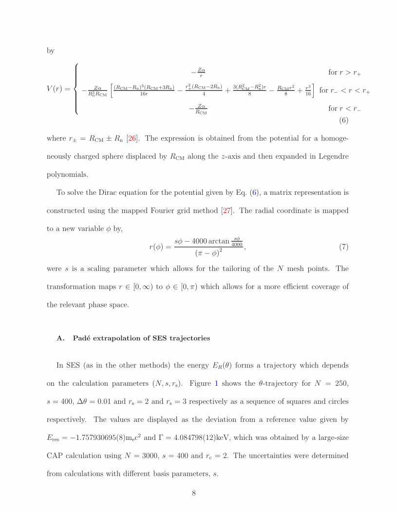
by

V (r) =

−Zαr

for r > r+

− ZαR3

nRCM

[

(RCM−Rn)3(RCM+3Rn)16r

−r2+(RCM−2Rn)

4+

3(R2CM−R2

n)r

8− RCMr2

8+ r3

16

]

for r− < r < r+

− ZαRCM

for r < r−

(6)

where r± = RCM ± Rn [26]. The expression is obtained from the potential for a homoge-

neously charged sphere displaced by RCM along the z-axis and then expanded in Legendre

polynomials.

To solve the Dirac equation for the potential given by Eq. (6), a matrix representation is

constructed using the mapped Fourier grid method [27]. The radial coordinate is mapped

to a new variable φ by,

r(φ) =sφ− 4000 arctan sφ

4000

(π − φ)2, (7)

were s is a scaling parameter which allows for the tailoring of the N mesh points. The

transformation maps r ∈ [0,∞) to φ ∈ [0, π) which allows for a more efficient coverage of

the relevant phase space.

A. Pade extrapolation of SES trajectories

In SES (as in the other methods) the energy ER(θ) forms a trajectory which depends

on the calculation parameters (N, s, rs). Figure 1 shows the θ-trajectory for N = 250,

s = 400, ∆θ = 0.01 and rs = 2 and rs = 3 respectively as a sequence of squares and circles

respectively. The values are displayed as the deviation from a reference value given by

Eres = −1.757930695(8)mec2 and Γ = 4.084798(12)keV, which was obtained by a large-size

CAP calculation using N = 3000, s = 400 and rc = 2. The uncertainties were determined

from calculations with different basis parameters, s.

8

0

0.005

0.010

0.015

0.020

0.025

0.030

-1.0 -0.5 0 0.5 1.0 1.5 2.0 2.5 3.0 3.5 4.0

∆Γ (

keV

)

∆Eres (10-5 mec2 )

Figure 1: (Color Online) The Γ(1Sσ) resonance θ-trajectory from N = 250, rs = 2 (red squares)

and rs = 3 (blue circles) displayed as the difference from a reference calculation (cf. text) for

the U-Cf system at R = 20 fm in monopole approximation. The ×’s mark the resonance energy

obtained by minimizing∣

∣

∣

dER

dθ

∣

∣

∣. The Np = 8 data points used for the extrapolations are bracketed

by the solid symbols, and a spacing of ∆θ = 0.01 was used.

In Fig. 1, the ER(θ) results for small θ values start in the upper right hand and abruptly

change direction after a few points. This happens in the vicinity of the reference value given

by the point (0,0). As θ increases beyond the cusp in the trajectory, ER(θ) changes more

slowly, and the θ-trajectory points become denser. Due to the finite number of collocation

points N , the actual value of θcrit (the minimum θ value such that ψres is bounded and

properly represented within the finite basis) is higher than theoretically predicted [14], and

is close to the cusp-like behavior in the θ-trajectory.

Optimal, directly calculated, approximate values for the resonance energy are chosen by

finding the minimum of∣

∣

dER

dθ

∣

∣

θ=θopt[13, 14], and are displayed as black crosses for both

9

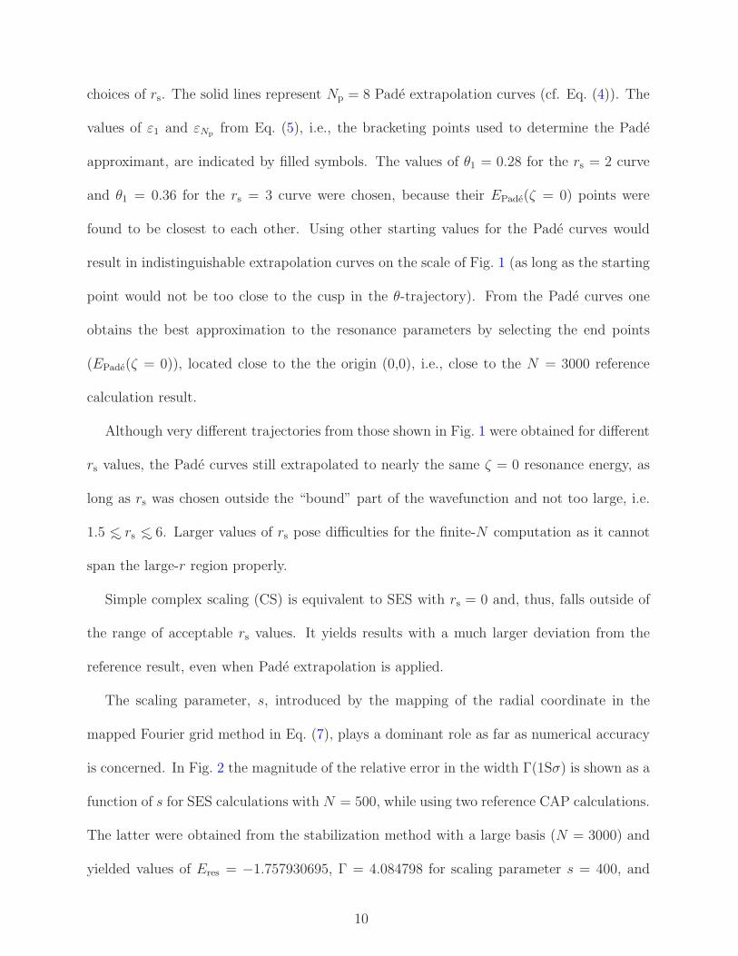
choices of rs. The solid lines represent Np = 8 Pade extrapolation curves (cf. Eq. (4)). The

values of ε1 and εNpfrom Eq. (5), i.e., the bracketing points used to determine the Pade

approximant, are indicated by filled symbols. The values of θ1 = 0.28 for the rs = 2 curve

and θ1 = 0.36 for the rs = 3 curve were chosen, because their EPade(ζ = 0) points were

found to be closest to each other. Using other starting values for the Pade curves would

result in indistinguishable extrapolation curves on the scale of Fig. 1 (as long as the starting

point would not be too close to the cusp in the θ-trajectory). From the Pade curves one

obtains the best approximation to the resonance parameters by selecting the end points

(EPade(ζ = 0)), located close to the the origin (0,0), i.e., close to the N = 3000 reference

calculation result.

Although very different trajectories from those shown in Fig. 1 were obtained for different

rs values, the Pade curves still extrapolated to nearly the same ζ = 0 resonance energy, as

long as rs was chosen outside the “bound” part of the wavefunction and not too large, i.e.

1.5 ∼< rs ∼< 6. Larger values of rs pose difficulties for the finite-N computation as it cannot

span the large-r region properly.

Simple complex scaling (CS) is equivalent to SES with rs = 0 and, thus, falls outside of

the range of acceptable rs values. It yields results with a much larger deviation from the

reference result, even when Pade extrapolation is applied.

The scaling parameter, s, introduced by the mapping of the radial coordinate in the

mapped Fourier grid method in Eq. (7), plays a dominant role as far as numerical accuracy

is concerned. In Fig. 2 the magnitude of the relative error in the width Γ(1Sσ) is shown as a

function of s for SES calculations with N = 500, while using two reference CAP calculations.

The latter were obtained from the stabilization method with a large basis (N = 3000) and

yielded values of Eres = −1.757930695, Γ = 4.084798 for scaling parameter s = 400, and

10

Eres = −1.757930702, Γ = 4.084808 for s = 750 respectively. Each SES data point was

10-7

10-6

10-5

10-4

10-3

10-2

0 500 1000 1500 2000

|∆Γ|

/Γ

s

Figure 2: (Color Online) Magnitude of relative error for Pade extrapolated widths ∆Γ(1Sσ) for

N = 500 as a function of the scaling parameter, s, for the U-Cf system at R = 20 fm in monopole

approximation. Data shown are obtained using two reference calculations from the stabilized CAP

method with N = 3000 and rc = 2; red plus symbols: s = 400; blue squares: s = 750 (cf. text).

obtained by finding the closest intersection of the rs = 2, 3, 4 Pade curves from all starting

θ’s (for θ > θcrit), and taking the average of these three best values. The use of different rs

values within the acceptable range would cause changes too small to see on this plot. The

resonance position, Eres, is much more stable with respect to s and therefore not shown.

The technique of combining information from different rs calculations in order to select

the ideal subset of θ points helps with the following problem. For each calculation with

fixed value of rs we looked at extrapolated values for the resonance width as a function of

the start value θi, and observed the deviation from the average value. It was found that

numerical noise present in the data was minimal for some range of θi values (different for each

11

calculation). This noise was investigated as a function of extrapolation order Np. Combining

information from calculations with different values of rs allowed us to eliminate two sources

of random uncertainties associated with finite-precision input to a sensitive extrapolation

calculation.

The results demonstrate that the extrapolated (θ = 0) SES N = 500 calculations exceed

the precision of the stabilized (non-extrapolated) N = 3000 CAP calculations. Table I gives

the resonance parameter results (Eres,Γ) for two different extrapolations, namely Np = 4, 8

for basis size N = 500, and mapping parameter 300 ≤ s ≤ 700, which corresponds to a

subset of the data shown in Fig. 2. The standard deviation of the mean,

σ =

Ni∑

i

√

(xi − x)2

Ni, (8)

where x is the average x-value, are given separately for resonance position and width. The

results are encouraging since extrapolation provides a marked improvement over the stabi-

lized CS method discussed in Ref. [4].

Np Eres σ(Eres) Γ (keV) σ(Γ)

8 -1.75793073 1.7×10−7 4.0848085 1.4×10−6

4 -1.75793072 1.6×10−7 4.0848031 1.4×10−6

Table I: Averaged resonance position and width from the extrapolated SES method with basis size

N = 500 using extrapolation orders Np = 8 and Np = 4. The values were averaged over the stable

range 300 ≤ s ≤ 700. The standard deviation of the mean is given by σ separately for position

and width.

12

B. Pade extrapolation of CAP trajectories

We have shown that a quadratic complex absorbing potential (cf. Eq. 2) gives better

results than simple complex scaling (CS) when used as a stabilization method [4]. We find

that the performance of SES represents an improvement over that of CS and it is competitive

with CAP.

Even for the same calculation parameters (N, s, rc), the η-trajectory for CAP is found

to be different from the θ trajectory in SES. Figure 3 shows a trajectory pair for identical

calculation parameters, namely N = 500, s = 600, and rs = rc = 3 respectively. Even

-0.002

-0.001

0

0.001

0.002

0.003

0.004

-1.5 -1.0 -0.5 0 0.5

∆Γ (

keV

)

∆Eres (10-6 mec2 )

Figure 3: (Color Online) SES θ-trajectory with N = 500, s = 600, rs = 3 (blue circles), and

CAP η-trajectory for N = 500, s = 600, rc = 3 (red diamonds) displayed as the difference from a

reference calculation for the 1Sσ state in the U-Cf system at R = 20 fm in monopole approximation.

The ×’s mark the approximate values obtained from the stabilization method. The reference value

was obtained by Pade extrapolation of CAP calculations with N = 3000, Np = 4 for rc = 2, 3, 4

yielding Eres = −1.7579307062(5)mec2 and Γ = 4.08481303(8)keV.

13

though the trajectories are rather different, the Pade curves extrapolate to rather close values

(EPade(η = 0)) as (EPade(θ = 0)) from the SES method, i.e. the extrapolated resonance

parameters for both methods are very similar. When looking at plots of the N = 500 η = 0

extrapolation results for CAP as a function of s, as was done in Fig. 2 for SES, we observe

almost identical results. In table II, the average and standard deviation of the mean, σ

(cf. Eq. 8), for the CAP results for N = 500, 300 ≤ s ≤ 700 are given for two different

extrapolation sizes, Np = 4, 8.

Np Eres σEres Γ (keV) σΓ

8 -1.75793072 1.6×10−7 4.0848141 3.1×10−6

4 -1.75793072 1.7×10−7 4.0848122 5.4×10−6

Table II: Same as in Table I, but for the extrapolated CAP method with basis size N = 500.

C. Comparison of CAP and SES results

Both methods (CAP and SES) show similar behavior with respect to different aspects of

the calculation. Both are relatively insensitive to the number of Pade points, Np, used in

the extrapolation. It was found that the results were unchanged, to the relevant precision,

for 4 ≤ Np ≤ 12. The effects of changing the distance between the analytic continuation

parameter (∆θ for SES and ∆η for CAP) were similarly found to be small compared with

s.

It was found that one could choose optimal ζi start values for the Pade approximation

by minimizing the deviation between ER(ζ = 0) from different rs or rc calculations. This is

simple to implement, and works well for different values ofNp. In this way one obtains results

that are independent of the starting point for the rotation (rs in SES) or the imaginary

14

potential (rc in CAP). The results are therefore very stable with respect to the analytic

continuation parameters and depend only on the parameters from the mapped Fourier grid

method. As shown in Fig. 2 for SES (a very similar graph was obtained for CAP), there is

a range of s for which results are stable. For larger basis size N the stable s-range increases

making a judicious choice of s less important.

We have averaged the results from both the SES and CAP methods over the stable s

region, for a basis size of N = 500 in tables I & II. The standard deviation for the width σ(Γ)

within either method is below 10−5, while the results differ at this level. It is, therefore, of

interest to determine the reliability of the error estimate which is based upon basis parameter

variations using larger-N extrapolated calculations. Comparison of the width results with

such an estimate based upon N = 3000 CAP and SES calculations indicates that SES and

CAP converge to the same value, closest to the CAP value given in table II.

Concerning the most appropriate order for the extrapolations it is worth noting that the

CAP Pade trajectories are rather straight in comparison with the ones for SES, and Np = 4

might be more appropriate in this case. Nevertheless, we find no systematic improvement

when going to the lower-order approximation (which might be deemed more stable with

respect to numerical noise in the trajectory points).

IV. COUPLED-CHANNEL CALCULATIONS

The ability to compute the resonance parameters to high precision with moderate basis

size (e.g., N = 500) allows us to explore the effects of higher multipoles which are present

in the two-center interaction. We are not aware of prior investigations of such coupled-

channel resonance calculations of supercritical Dirac states. While the effect on the resonance

position is expected to be small, the sensitivity of the width to computational details (cf.

15

the different results discussed in [4]) indicates that some broadening of the resonance may

occur.

To account for such two-center potential effects the wavefunction is expanded using spinor

spherical harmonics, χκ,µ,

Ψµ(r, θ, φ) =∑

κ

Gκ(r)χκ,µ(θ, φ)

iFκ(r)χ−κ,µ(θ, φ)

, (9)

which are labeled by the relativistic angular quantum number κ (analogous to l in non-

relativistic quantum mechanics) and the magnetic quantum number µ [3]. The Dirac

equation for the scaled radial functions, f(r) = rF (r) and g(r) = rG(r), then becomes

(~ = c = 1),

dfκ

dr−κ

rfκ = − (E − 1) gκ +

±∞∑

κ=±1

〈χκ,µ |V (r, R)|χκ,µ〉gκ , (10)

dgκ

dr+κ

rgκ = (E + 1) fκ −

±∞∑

κ=±1

〈χ−κ,µ |V (r, R)|χ−κ,µ〉fκ , (11)

where V (r, R) is the potential for two uniformly charged spheres displaced along the z-axis,

which is expanded into Legendre polynomials according to V (r, R) =∑∞

l=0 Vl(r, R)Pl(cos θ)

[3]. The monopole term, V0, is given explicitly in Eq. (6), and for the present work we include

the coupling terms required for the κ = ±1,−2 channels (i.e., the V1(r, R)〈χ±κ,µ |P1|χ±κ,µ〉

dipole and V2(r, R)〈χ±κ,µ |P2|χ±κ,µ〉 quadrupole terms). The κ = 1,−2 channels (P1/2 and

P3/2 respectively) have the strongest coupling to the κ = −1 (S-states) and are therefore

expected to have the largest impact on the supercritical ground state.

Table III gives the 1Sσ resonance parameters for different internuclear separations for

both the one- and three-channel CAP calculations. The CAP calculations were performed

using a basis size of N = 500 per channel with 300 ≤ s ≤ 700. The CAP parameters of

rc = 2, 3, 4 were used to obtain the most stable θ range for extrapolation, which was carried

16

R(fm)

Single-channel (κ = −1) Three-channel (κ = −1, 1, 2) |Γ1−Γ3|Γ1

Eres (mc2) Γ1 (keV) Eres (mc2) Γ3 (keV) (×10−3)

16 -2.00635363(3) 8.148233(4) -2.00646180(3) 8.150153(3) 0.236

18 -1.87487669(4) 5.881605(1) -1.87502343(4) 5.883977(2) 0.403

20 -1.75793073(4) 4.0848148(4) -1.75811259(4) 4.087394(1) 0.631

22 -1.65393272(3) 2.708987(1) -1.65414448(3) 2.711524(2) 0.937

24 -1.5612122(1) 1.6966694(3) -1.56144826(1) 1.698947(1) 1.34

26 -1.47820830(4) 0.9877052(4) -1.47846358(4) 0.989571(1) 1.89

28 -1.40354329(5) 0.5221621(4) -1.40381341(4) 0.523544(1) 2.65

30 -1.33603643(6) 0.2420749(2) -1.33631779(6) 0.242976(1) 3.72

32 -1.27469286(5) 0.0931429(1) -1.27498253(5) 0.093639(5) 5.32

34 -1.21868219(5) 0.0271161(1) -1.21897787(4) 0.027322(2) 7.59

36 -1.16731491(6) 0.0050374(1) -1.16761472(7) 0.005091(2) 10.7

38 -1.12001745(6) 0.0004170(3) -1.12031983(6) 0.000439(4) 52.5

Table III: Averaged 1Sσ resonance position and width from the extrapolated CAP method with

basis size N = 500, Np = 4, for single-channel (monopole) and three-channel calculations as a

function of separation, R, in the U-Cf system. The values were averaged over the stable range

300 ≤ s ≤ 700 using rc = 2, 3, 4. The value in parenthesis represents the standard deviation from

the average and the last column gives the relative difference of the width from three- to one-channel.

out with order Np = 4. Values in parentheses indicate the standard deviation of the mean

(cf. Eq. 8). We note that the accuracy of the calculations - as indicated by the deviation -

is much higher than what is required to measure the effect of the the P-state channels on

the 1Sσ resonance.

17

The final column contains the relative difference of the width between the three-channel

results and the monopole approximation. The correction due to the dipole and quadrupole

potentials is seen to increase with internuclear separation R. This trend can be expected,

as the overall interaction becomes less spherically symmetric in this limit. The effect is

small, however, as the strongest contribution towards the binding energy (and thus the

supercriticality) is provided by the monopole part. The dipole interaction contributions

to the resonance parameters are a result of the relatively small charge asymmetry in the

U92+-Cf98+ potential. Quadrupole couplings to D states can be expected to generate more

significant changes in Eres and Γ.

V. DISCUSSION

We have extended the method of smooth exterior scaling (SES) to the relativistic Dirac

equation. For both the addition of a complex absorbing potential (CAP) and SES, we have

also shown that by extrapolation of the complex energy eigenvalue trajectories which are

functions of the analytic continuation parameter, ζ , to ζ = 0 using appropriate ζ-trajectory

values (cf. section IIC), one obtains an accurate and robust estimation of the resonance

parameters. These results use much smaller basis than would be required for similar pre-

cision using stabilization. While adding the extrapolation adds new parameters, we found

minimizing the distance between extrapolated results for different calculation parameters

was a simple and highly effective method of reducing the parameter space. The effects of

the number of calculation points, Np, was found to be very small provided it was in the

range 4 ≤ Np ≤ 12.

The effects of higher order terms and the P -states were explored and found to have a in-

creasing influence as the two-center system becomes less spherically symmetric which occurs

18

at larger internuclear separations R. The resonances could acquire additional broadenings

and shifts from dynamical effects not included in the quasi-static approximation.

VI. ACKNOWLEDGMENTS

This work was supported by NSERC Canada, and was carried out using the Shared

Hierarchical Academic Research Computing Network (SHARCNET:www.sharcnet.ca). E.

Ackad was supported by the Ontario Graduate Scholarship program.

[1] J. Reinhardt, B. Muller, and W. Greiner, Phys. Rev. A 24, 103 (1981).

[2] J. Rafelski, L. Fulcher, and A. Klein, Phys. Rep. 38, 227 (1978).

[3] W. Greiner, Relativistic Quantum Mechanics: Wave Equations (Springer, 2000), 3rd ed.

[4] E. Ackad and M. Horbatsch, Phys. Rev. A 75, 022508 (2007).

[5] R. Lefebvre, M. Sindelka, and N. Moiseyev, Phys. Rev. A 72, 052704 (2005).

[6] M. Ingr, H.-D. Meyer, and L. S. Cederbaum, J. Phys. B 32, L547 (1999).

[7] R. Santra, R. W. Dunford, and L. Young, Phys. Rev. A 74, 043403 (2006).

[8] R. Santra and L. S. Cederbaum, J. Chem. Phys. 117, 5511 (2002).

[9] S. Sahoo and Y. K. Ho, J. Phys. B 33, 2195 (2000).

[10] U. V. Riss and H.-D. Meyer, J. Phys. B 26, 4503 (1993).

[11] I. A. Ivanov and Y. K. Ho, Phys. Rev. A 69, 023407 (2004).

[12] I. B. Muller, R. Santra, and L. S. Cederbaum, Int. J. Quant. Chem. 94, 75 (2003).

[13] W. P. Reinhardt, Ann. Rev. Phys. Chem. 33, 223 (1982).

[14] N. Moiseyev, Phys. Rep. 302, 211 (1998).

19

[15] T. N. Rescigno, M. Baertschy, W. A. Isaacs, and C. W. McCurdy, Science 286, 2474 (1999).

[16] J. Royal and A. E. Orel, Phys. Rev. A 73, 042706 (2006).

[17] J. Rao, W. Liu, and B. Li, Phys. Rev. A 50, 1916 (1994).

[18] A. Igarashi and I. Shimamura, Phys. Rev. A 70, 012706 (2004).

[19] A. D. Alhaidari, Phys. Rev. A 75, 042707 (2007).

[20] G. D. Doolen, Journal of Physics B: Atomic and Molecular Physics 8, 525 (1975).

[21] P. R. C. N. Moiseyev and F. Weinhold, Mol. Phys. 36, 1613 (1978).

[22] R. Santra, Phys. Rev. A 74, 034701 (2006).

[23] H. O. Karlsson, J. Chem. Phys. 109, 9366 (1998).

[24] U. V. Riss and H.-D. Meyer, Journal of Physics B: Atomic, Molecular and Optical Physics

31, 2279 (1998).

[25] L. Schlessinger, Phys. Rev. 167, 1411 (1966).

[26] G. Soff, W. Betz, J.Reinhardt, and J. Rafelski, Phys. Scr. 17, 417 (1978).

[27] E. Ackad and M. Horbatsch, J. Phys. A 38, 3157 (2005).

20