Supercontinuum generation in the picosecond regime - qowiki

Supercontinuum generation in thepicosecond regime

Arthur Zonnenberg

September 12, 2006

Contents

1. Introduction and Motivation 3

2. Theory 42.1. Fiber Design . . . . . . . . . . . . . . . . . . . . . . . . . . . . . . . . . . 42.2. Conventional Fiber Optics . . . . . . . . . . . . . . . . . . . . . . . . . . 52.3. Dispersion . . . . . . . . . . . . . . . . . . . . . . . . . . . . . . . . . . . 52.4. Nonlinear Processes . . . . . . . . . . . . . . . . . . . . . . . . . . . . . . 7

2.4.1. Self Phase Modulation . . . . . . . . . . . . . . . . . . . . . . . . 72.4.2. Four Wave Mixing . . . . . . . . . . . . . . . . . . . . . . . . . . 92.4.3. The Nonlinear Schrodinger Equation . . . . . . . . . . . . . . . . 122.4.4. Solitons . . . . . . . . . . . . . . . . . . . . . . . . . . . . . . . . 13

3. Experimental Setup 153.1. Fiber Parameters . . . . . . . . . . . . . . . . . . . . . . . . . . . . . . . 163.2. Pump Setup . . . . . . . . . . . . . . . . . . . . . . . . . . . . . . . . . . 163.3. Collection and Analysis Setup . . . . . . . . . . . . . . . . . . . . . . . . 18

4. Results 204.1. Polarization Dependence . . . . . . . . . . . . . . . . . . . . . . . . . . . 204.2. Wavelength Dependence . . . . . . . . . . . . . . . . . . . . . . . . . . . 224.3. Power Dependence . . . . . . . . . . . . . . . . . . . . . . . . . . . . . . 26

4.3.1. Zero-Dispersion Regime . . . . . . . . . . . . . . . . . . . . . . . 264.3.2. Anomalous Dispersion Regime . . . . . . . . . . . . . . . . . . . . 29

5. Discussion 345.1. Results Obtained with a FWM Model . . . . . . . . . . . . . . . . . . . . 345.2. Results Obtained with a Soliton Model . . . . . . . . . . . . . . . . . . . 36

6. Conclusion 37

A. Tables 40

2

Abstract

In this report a 6m NL-PM-750 fiber is pumped with 2 ps pulses from a mode-locked Ti-sapphire laser to generate a spectrally broad supercontinuum. Polarization, wavelengthand power dependence of the generated supercotinua are measured. These results arethen compared to two different models; one based on four wave mixing (FWM), theother based on solitons as the primary process for generating new spectral components.The FWM model is not adequate to describe the observed spectra. The soliton modeluses a Raman-induced soliton self-frequency shift, couples solitons to dispersive wavesand gives a better description of observed picosecond supercontinua.

1. Introduction and Motivation

A small, point-like illuminating source can be used to perform transmission and reflectionmeasurements on a small object, such as a 50x50 µm sample. A supercontinuum is aspectrum with a broad spectral range. Supercontinua generated via nonlinear opticalprocesses in photonic crystal fibers (PCFs) are bright - up to 3 orders of magnitudelarger than an incandescent lamp [1] - and come at a small size (typically 1 to 10 µm).The goal is to generate a broadband spectrum at 750 and 1500 nm using a PCF. Thisfiber is specified to have two zero order dispersion wavelengths (one at 750 nm andone at 1260 nm) and is able to generate broadband spectra around those wavelengthsusing nonlinear processes. This bachelor research project has been performed with thoseobjectives in mind, while gaining a better understanding of supercontinuum generation.

3

2. Theory

In this chapter a brief overview is given to cover the theory necessary to understandphotonic crystal fibers (PCFs). The fiber design is explained in section 2.1. Linearoptical properties and modal solutions are discussed in section 2.2. Fiber dispersionis so important it gets its own section 2.3, while nonlinear processes are introduced insection 2.4.

2.1. Fiber Design

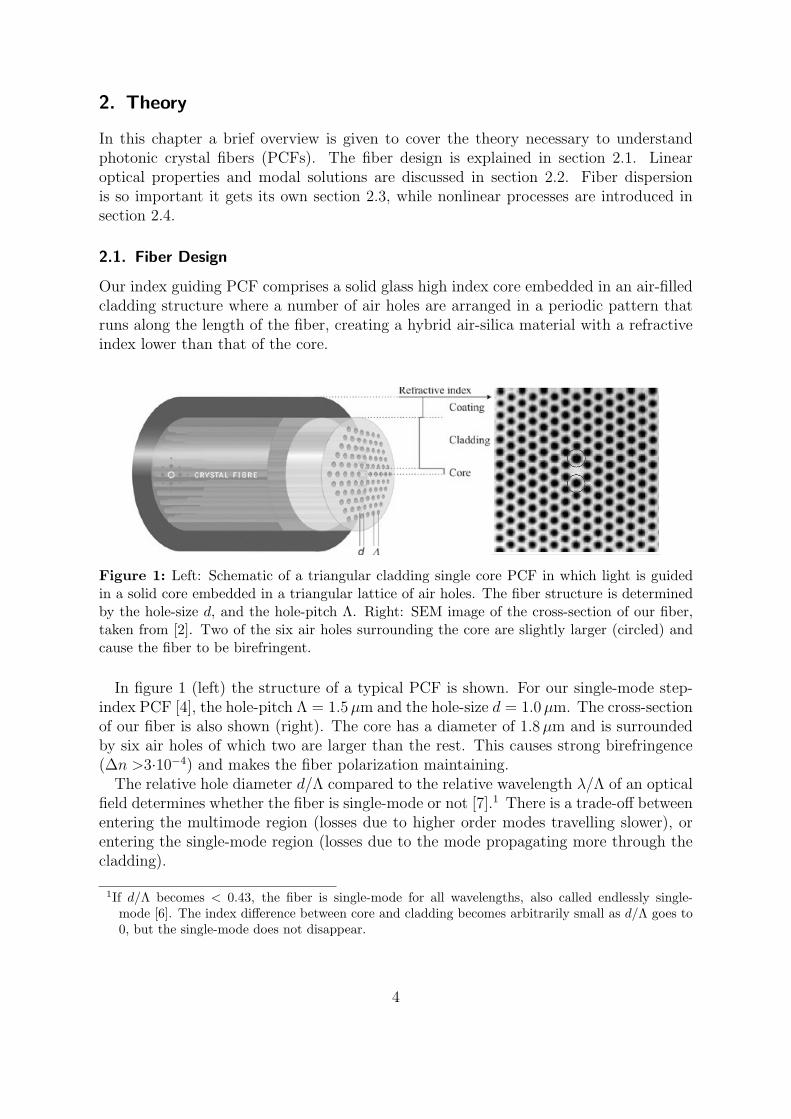
Our index guiding PCF comprises a solid glass high index core embedded in an air-filledcladding structure where a number of air holes are arranged in a periodic pattern thatruns along the length of the fiber, creating a hybrid air-silica material with a refractiveindex lower than that of the core.

Figure 1: Left: Schematic of a triangular cladding single core PCF in which light is guidedin a solid core embedded in a triangular lattice of air holes. The fiber structure is determinedby the hole-size d, and the hole-pitch Λ. Right: SEM image of the cross-section of our fiber,taken from [2]. Two of the six air holes surrounding the core are slightly larger (circled) andcause the fiber to be birefringent.

In figure 1 (left) the structure of a typical PCF is shown. For our single-mode step-index PCF [4], the hole-pitch Λ = 1.5 µm and the hole-size d = 1.0 µm. The cross-sectionof our fiber is also shown (right). The core has a diameter of 1.8 µm and is surroundedby six air holes of which two are larger than the rest. This causes strong birefringence(∆n >3·10−4) and makes the fiber polarization maintaining.

The relative hole diameter d/Λ compared to the relative wavelength λ/Λ of an opticalfield determines whether the fiber is single-mode or not [7].1 There is a trade-off betweenentering the multimode region (losses due to higher order modes travelling slower), orentering the single-mode region (losses due to the mode propagating more through thecladding).

1If d/Λ becomes < 0.43, the fiber is single-mode for all wavelengths, also called endlessly single-mode [6]. The index difference between core and cladding becomes arbitrarily small as d/Λ goes to0, but the single-mode does not disappear.

4

For our fiber the values of d and Λ ensure a good single-mode operation and putthe cutoff wavelength for multi-mode operation ≤ 650 nm. The cutoff wavelength of asingle-mode fiber is the wavelength above which the fiber propagates only the funda-mental mode. The fundamental mode can never be cut off [9].

2.2. Conventional Fiber Optics

Some insight into the properties of a PCF can be gained by treating the fiber as a con-ventional optical fiber. A conventional (step-index profile) fiber has a dielectric constantε(−→r , ω) which is high within the core r ≤ a (with a the core radius) and low in thecladding r > a. Electromagnetic waves propagating through a fiber are described by theHelmholtz equation ( [10], p. 501):

∇2E(−→r , ω) + ε(−→r , ω)ω2

c2E(−→r , ω) = 0, (2.1)

The Helmholtz equation can be solved for the fiber geometry using the method of sepa-ration of variables. We introduce

E(−→r , ω) = F (x, y) exp(iβ(ω)z) (2.2)

for a solution propagating in the positive z direction. For the part perpendicular topropagation this leads to

∂2F

∂x2+

∂2F

∂y2+

(ε(−→r , ω)

ω2

c2− β2(ω)

)F = 0 (2.3)

where r =√

x2 + y2. The introduced β can be interpreted as a wavenumber of thesolution, and gives the phase velocity in the z-direction. Equation 2.3 can be solved incylindrical coordinates and yields Bessel functions inside the core and Neumann functionsin the cladding. We will limit ourselves to a single propagation constant β, assumingthat we are dealing with a single-mode fiber ( [11], pp. 31-37; [12]).

2.3. Dispersion

Dispersion is the effect that the propagation constant β depends on ω. Dispersion playsan important role in pulse propagation because different spectral components of thepulse travel at different phase velocities given by ω/β. This is caused by two differentcontributions: material dispersion and waveguide dispersion.

Material dispersion reflects the fact that the refractive index of a material is frequencydependent, i.e. high-frequency (blue) components of an optical pulse travel slower thanlow-frequency (red) components of the same pulse. Each ω has its own modal distribu-tion F (x, y), part of which is in the core, and part of which is in the cladding. Waveguidedispersion is then the effect that due to the different modal distributions, the effective

5

index and therefore the propagation constant differ for different frequencies ω.

We define the derivatives of the propagation constant as:

βm(ω) =dmβ(ω)

dωm(m = 0, 1, 2, . . . ) (2.4)

The parameters 1/β1 and 1/β2 are known as the group velocity and the group velocitydispersion. An optical pulse, centered around the group frequency ω0, moves at thegroup velocity 1/β1. The group velocity dispersion gives the spreading of the pulse inthe temporal domain.

For wavelengths for which the fiber is said to exhibit normal dispersion (β2 > 0),high-frequency (blue) components of an optical pulse travel slower than low-frequency(red) components of the same pulse. By contrast, the opposite occurs in the anomalousdispersion regime (β2 < 0).

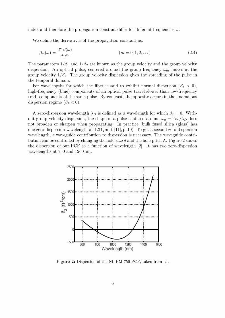
A zero-dispersion wavelength λD is defined as a wavelength for which β2 = 0. With-out group velocity dispersion, the shape of a pulse centered around ω0 = 2πc/λD doesnot broaden or sharpen when propagating. In practice, bulk fused silica (glass) hasone zero-dispersion wavelength at 1.31 µm ( [11], p. 10). To get a second zero-dispersionwavelength, a waveguide contribution to dispersion is necessary. The waveguide contri-bution can be controlled by changing the hole-size d and the hole-pitch Λ. Figure 2 showsthe dispersion of our PCF as a function of wavelength [2]. It has two zero-dispersionwavelengths at 750 and 1260 nm.

Figure 2: Dispersion of the NL-PM-750 PCF, taken from [2].

6

The measured [2] dispersion of our fiber (figure 2) can be approximated by a polyno-mial. This function can be found by fitting the dispersion curve to a polynomial of ordern. We use a second order polynomial β2 = a+bω+cω2 and a least squares fitting methodto determine the constants a, b and c. This gives the simplest mathematical form of β2

that has two zero-dispersion wavelengths. To get a more accurate approximation of β2

we also use a sixth order polynomial β2 = a + bω + cω2 + dω3 + eω4 + fω5 + gω6. Thenumerical data and coefficients that were fitted are given in appendix A.

2.4. Nonlinear Processes

In this section nonlinear processes relevant for supercontinuum generation are described.Self and cross phase modulation are described in section 2.4.1, followed by four wavemixing 2.4.2. Introducing the nonlinear change in refractive index leads to the nonlinearSchrodinger equation in section 2.4.3, under certain assumptions and approximations.When the contributions of self phase modulation and the nonlinear response to dispersioncancel each other, soliton solutions are found in section 2.4.4. Solitons in turn can befrequency shifted and coupled to dispersive waves.

2.4.1. Self Phase Modulation

Self phase modulation (SPM) is a nonlinear optical effect of light propagating througha dispersive medium. A high intensity pulse of light will induce a varying refractiveindex of the medium due to the optical Kerr effect. This variation in refractive indexwill produce a phase shift in the pulse, leading to a change in the frequency spectrumof the pulse.

Let us consider the propagation of the optical pulse

E(z, t) = A(z, t) exp i(ω0t− β0z) + c.c. (2.5)

with β0 = n0ω0

cthrough a medium characterized by a nonlinear refractive index of the

sort

n(t) = n0 + n2I(t), (2.6)

where I(t) is the intensity and n2 is the nonlinear refractive index. Note that for thepresent we are assuming that the medium can respond essentially instantaneously tothe pulse intensity. We also assume that the nonlinear medium is sufficiently short thatno reshaping of the optical pulse can occur within the medium; the only effect of themedium is to change the refractive index n0 to n(t) in the instantaneous phase of thetransmitted pulse:

φ(t) = ω0t− n(t)ω0z

c⇒ ∆φ(t) = −n2ω0z

cI(t) (2.7)

where ω0 is the (vacuum) center wavelength of the pulse, and z is the distance the pulsehas propagated (in our case equal to the fiber length L). It is then intuitive to describe

7

the spectral content of the transmitted pulse by introducing the instantaneous frequencyω(t) of the pulse,

ω(t) =dφ(t)

dt= ω0 − n2ω0z

c

dI(t)

dt(2.8)

where the variation in frequency depends on the phase shift. This concept is well-definedand given by this equation whenever the amplitude A(t) varies slowly compared to anoptical period. As an example we consider a pulse with intensity given by

I(t) = I0 exp

(− t2

τ 2

)(2.9)

with τ the pulse width. The result is

ω(t) = ω0 +n2ω0z

c

2t

τ 2I(t) ⇒ ∆ω(t) =

2t

τ 2∆φ(t) (2.10)

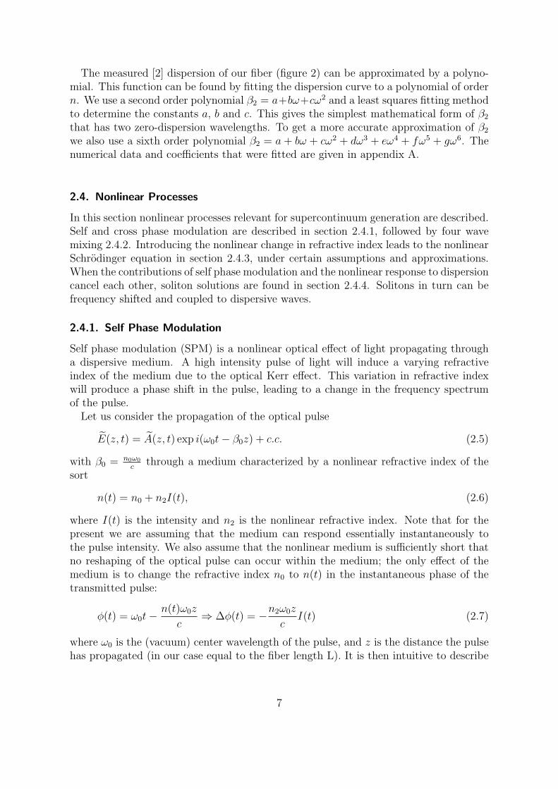
and plotted in figure 3.

Figure 3: SPM for a Gaussian shaped pulse. The front of the pulse is shifted to lowerfrequencies, the back to higher frequencies. In the center the shift is approximately linear.Image taken from Wikipedia [5].

The phase shift ∆φ(t) in equation 2.7 is set to 2π when the propagated distance z isequal to the nonlinear length LNL, defined as

LNL = (γP0)−1, (2.11)

8

where P0 is the peak power (P0/Aeff = I0).2 For our fiber γ = 95 (Wkm)−1. For a 2 ps

pulse, with a 1 nJ pulse energy3, the peak power P0 is roughly estimated as 1 nJ/2 ps =500W. This gives a nonlinear length (γP0)

−1 of 2.1 cm, clearly smaller than our fiberlength of L = 6 m.

The frequency shift in equation 2.10 can be written as

∆ω(t) =n2ω0z

cI0

2t

τ 2exp

(− t2

τ 2

)=

L

LNL

2t

τ 2exp

(− t2

τ 2

)(2.12)

This expression is maximal when t =±τ/√

2; for τ we take a pulse width of 2 ps, resultingin a frequency shift of ∆ω = ±0.12·1015. This corresponds to a spectral broadening of±45 nm for λ0 = 754 nm, for our 6 m fiber.

Cross Phase Modulation

When two or more optical pulses propagate simultaneously through a fiber, they inter-act with each other in a similar manner through the fiber nonlinearity. If two carrierfrequencies ω1 and ω2 are considered, the resulting nonlinear phase shift is given as( [11], p. 262)

φNL,j(z) = −n2ω0z

c(|Ej|2 + 2|E3−j|2) (2.13)

where j = 1 or 2. The second term on the right-hand side is the XPM term and is twiceas effective as SPM for the same intensity. Its origin can be traced back to the numberof terms that contribute to the triple sum implied in the nonlinear polarization4

PNL(r, t) = ε0χ(3)...E(r, t)E(r, t)E(r, t) (2.14)

When frequencies are non-degenerate the number of terms in the sum doubles for eachfrequency. The result of the XPM nonlinear phase shift is an asymmetric spectralbroadening.

2.4.2. Four Wave Mixing

Four Wave Mixing (FWM) is a third order parametric process that can be quite efficientfor generating new waves. We consider four optical waves oscillating at frequenciesω1, ω2, ω3 and ω4 which are linearly polarized along the same axis x. For example,( [11], pp. 389-392; [14], pp. 245-252), 3 photons of the same frequency can produce a 4thphoton (3rd harmonic generation), or 2 photons of the same frequency can produce astokes and an anti-stokes photon (four wave mixing). Energy conservation for four wavemixing leads to:

ω1 + ω2 = ω3 + ω4 (2.15)

2The effective core area of Aeff = 2µm2 is already incorporated in γ.31 nJ corresponding to 80 mW average coupled power (see section 3.2) at a repetition rate of 80 MHz4D = ε0E + P, P = PL + PNL

9

The phase-matching condition for this process to occur is

∆β = β(ω1) + β(ω2)− β(ω3)− β(ω4) = 0 (2.16)

It is relatively easy to satisfy ∆β = 0 in the case that ω1 = ω2. This partially degeneratecase is the most relevant here: a strong pump wave at ω1 creates two sidebands locatedsymmetrically at frequencies ω3 and ω4 with a frequency shift

ΩS = ω1 − ω3 = ω4 − ω1 (2.17)

the low-frequency sideband at ω3 is also known as the Stokes or signal band, while thehigh-frequency sideband at ω4 is also known as the anti-Stokes or idler band.

If we rewrite equation 2.16 in terms of pump, source and idler we get

∆β = 2β(ωp)− β(ωs)− β(ωi) = 0 (2.18)

where the subscripts p, s and i stand for pump, signal and idler respectively. This equa-tion is our phase-matching condition and is used to predict the frequencies of the side-bands. First, we approximate β2 using the approximating polynomials from section 2.3.Second, we integrate β2(ω) twice with respect to ω to get the following function:

β(ω) + Bω + C (2.19)

where B and C are arbitrary integration constants. It is not difficult to show (withthe help of equation 2.15) that the integration constants do not matter for the phase-matching condition; B and C can therefore safely be set to zero. Physically, this corre-sponds to the fact that the nonlinear interaction is always phase-matched if the dispersionis linear. Finally, we numerically solve equation 2.18.

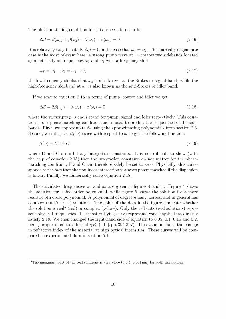
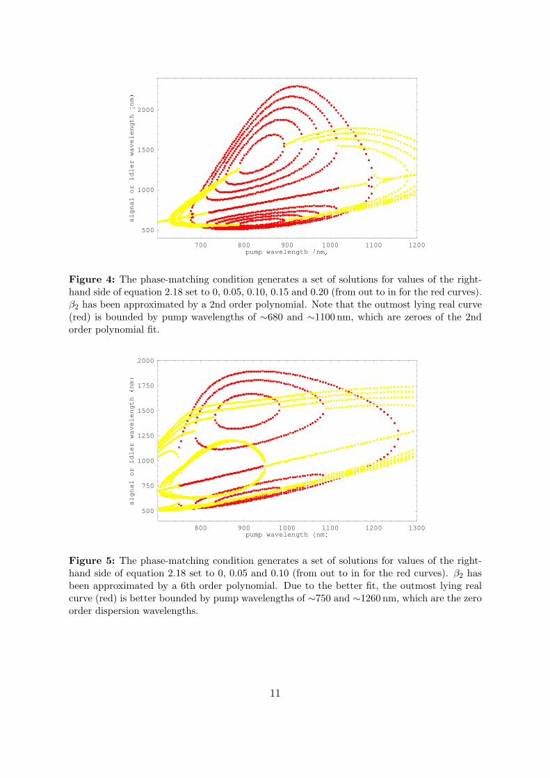
The calculated frequencies ωs and ωi are given in figures 4 and 5. Figure 4 showsthe solution for a 2nd order polynomial, while figure 5 shows the solution for a morerealistic 6th order polynomial. A polynomial of degree n has n zeroes, and in general hascomplex (and/or real) solutions. The color of the dots in the figures indicate whetherthe solution is real5 (red) or complex (yellow). Only the red dots (real solutions) repre-sent physical frequencies. The most outlying curve represents wavelengths that directlysatisfy 2.18. We then changed the right-hand side of equation to 0.05, 0.1, 0.15 and 0.2,being proportional to values of γP0 ( [11], pp. 394-397). This value includes the changein refractive index of the material at high optical intensities. These curves will be com-pared to experimental data in section 5.1.

5The imaginary part of the real solutions is very close to 0 (¡ 0.001 nm) for both simulations.

10

700 800 900 1000 1100 1200pump wavelength

nm

500

1000

1500

2000

la

ng

is

ro

re

ld

ih

tg

ne

le

va

w

mn

Figure 4: The phase-matching condition generates a set of solutions for values of the right-hand side of equation 2.18 set to 0, 0.05, 0.10, 0.15 and 0.20 (from out to in for the red curves).β2 has been approximated by a 2nd order polynomial. Note that the outmost lying real curve(red) is bounded by pump wavelengths of ∼680 and ∼1100 nm, which are zeroes of the 2ndorder polynomial fit.

800 900 1000 1100 1200 1300pump wavelength

nm

500

750

1000

1250

1500

1750

2000

la

ng

is

ro

re

ld

ih

tg

ne

le

va

w

mn

Figure 5: The phase-matching condition generates a set of solutions for values of the right-hand side of equation 2.18 set to 0, 0.05 and 0.10 (from out to in for the red curves). β2 hasbeen approximated by a 6th order polynomial. Due to the better fit, the outmost lying realcurve (red) is better bounded by pump wavelengths of ∼750 and ∼1260 nm, which are the zeroorder dispersion wavelengths.

11

2.4.3. The Nonlinear Schrodinger Equation

The nonlinear optical response of a fiber can be treated as a small perturbation. Ourfiber designed to have birefringence, and because of this it is polarization-maintaining.Therefore, the optical field is assumed to maintain its polarization along the fiber lengthso that a scalar approach is valid. Furthermore, the optical field is assumed to be quasi-monochromatic, i.e., the pulse spectrum, centered at ω0, is assumed to have a spectralwidth ∆ω such that ∆ω/ω0 ¿ 1. Since ω0 ∼1015 s−1 for visible light, this is valid forpulses as short as 10 fs (∆ω/ω0 = 0.05 for λ0 = 940 nm). This assumption is equivalentto saying that the amplitude of the pulse envelope is slowly varying due to the changingof phase velocities.

We neglect the Raman response of the medium ( [11], p. 40; [14], p. 375). In general,both electrons and nuclei respond to the optical field in a nonlinear manner. The nuclearresponse is inherently slower compared with the electronic response. For silica fibers thevibrational or Raman response occurs over a time scale of 60-70 fs. This is slow com-pared to the time scale of the electron response which is assumed to be instantaneous(i.e. response time = 0).

Using the above assumptions and approximations, equation 2.1 can be written as anequation in the propagation direction for a pulse with an amplitude A(z, ω). This isdone by assuming a solution of the form

E(−→r , ω) = A(z, ω)F (x, y) exp(iβ(ω)z) (2.20)

instead of equation 2.2 and by introducing the nonlinear response into ε(−→r , ω). Inaddition, higher order dispersion terms (β3, β4, etc.) are neglected and we work inthe frame of reference of an observer travelling with the group velocity (1/β1). Theresulting equation is known as the nonlinear Schrodinger equation (NLSE) ( [11], p. 44;[14], p. 280):

∂A

∂z+ 1

2iβ2

∂2A

∂t2= iγ|A|2A, (2.21)

with the nonlinear coefficient γ defined as:

γ =n2ω0

cAeff

(2.22)

where n2 is the nonlinear refractive index, neglecting absorption, Aeff is an effectivemode area and ω0 is the center frequency.6 The second term on the left-hand side ofequation 2.21 shows how pulses tend to spread due to group velocity dispersion, andthat the term on the right-hand side shows how pulses tend to spread due to self-phasemodulation (see section 2.4.1).

6It is possible to include higher order dispersion terms as well as the Raman effect into a similarpropagation equation. This is beyond the scope of this report

12

2.4.4. Solitons

It is possible for the effects of group velocity dispersion to compensate for the nonlin-ear effect (of self-phase modulation) if the group velocity dispersion is negative. Underappropriate conditions an optical pulse can indeed propagate through a dispersive, non-linear medium with an invariant shape. Such pulses are known as optical solitons. Asolution to equation 2.21 whose shape does not change is ( [14], p. 281)

A(z, τ) = A0sechτ

τ0

exp

(i−β2

2τ 20

z

)(2.23)

where the soliton pulse amplitude A0 and the soliton pulse width τ0 must be relatedaccording to

|A0|2 =−β2

γτ 20

(2.24)

β2 and γ must have opposite signs to represent a physical pulse. Because γ is always≥ 0, optical solitons can only exist in the anomalous dispersion regime (β2 < 0).

Soliton Self-Frequency Shift

In the derivation of the NLSE the response of the medium was assumed to be instanta-neous. However, the contributions to the nonlinearity from molecular vibrations (opticalphonons) is non-instantaneous and gives rise to the Raman effect. The Raman effectleads to a gain of the red frequency components relative to the blue frequency compo-nents of the pulse. This results in a red-shift of the whole pulse and is known as thesoliton self-frequency shift. The red-shift is strongest for the highest order soliton (cor-responding to the shortest pulse). This Raman-induced frequency shift can be writtenas ( [11], p. 186)

∆ωR(L) =−8|β2|TRL

15τ 40

(2.25)

where TR is a characteristic response time for the Raman gain, and τ0 is again the solitonwidth. Note that the frequency shift scales with β2 and fiber length L. To numericallycalculate the Raman effect on spectra, the NLSE needs to be expanded [17] [18].

Coupling to Dispersive Waves

Non solitonic radiation (NSR) can be emitted if a normal dispersive wave is phase-matched to a soliton via a four wave mixing process. The condition for this to happenis when ∆φ = φS − φNSR = 0. These phases of the soliton (S) and the dispersive wave(NSR) are given by [8]

φS =

(β(ωS) +

n2ωS|E|2c

)L− ωS

L

vg,S

(2.26)

13

φNSR = β(ωNSR)L− ωSL

vg,S

(2.27)

where vg,S is the group velocity of the soliton and L is the fiber length. The phasecondition ∆φ = 0 leads to

β(ωS) +n2ωS|E|2

c− β(ωNSR) = 0 (2.28)

and is actually independent of fiber length and group velocity. In principle this allowsus to predict in which part of the spectrum the NSR light will be generated.

14

3. Experimental Setup

ps Ti:SapphireLaser

USBSpectrometer

l/2ND Filter

60xMO

40xMO

Diaphragm 6m PCF

MMF 50 mm

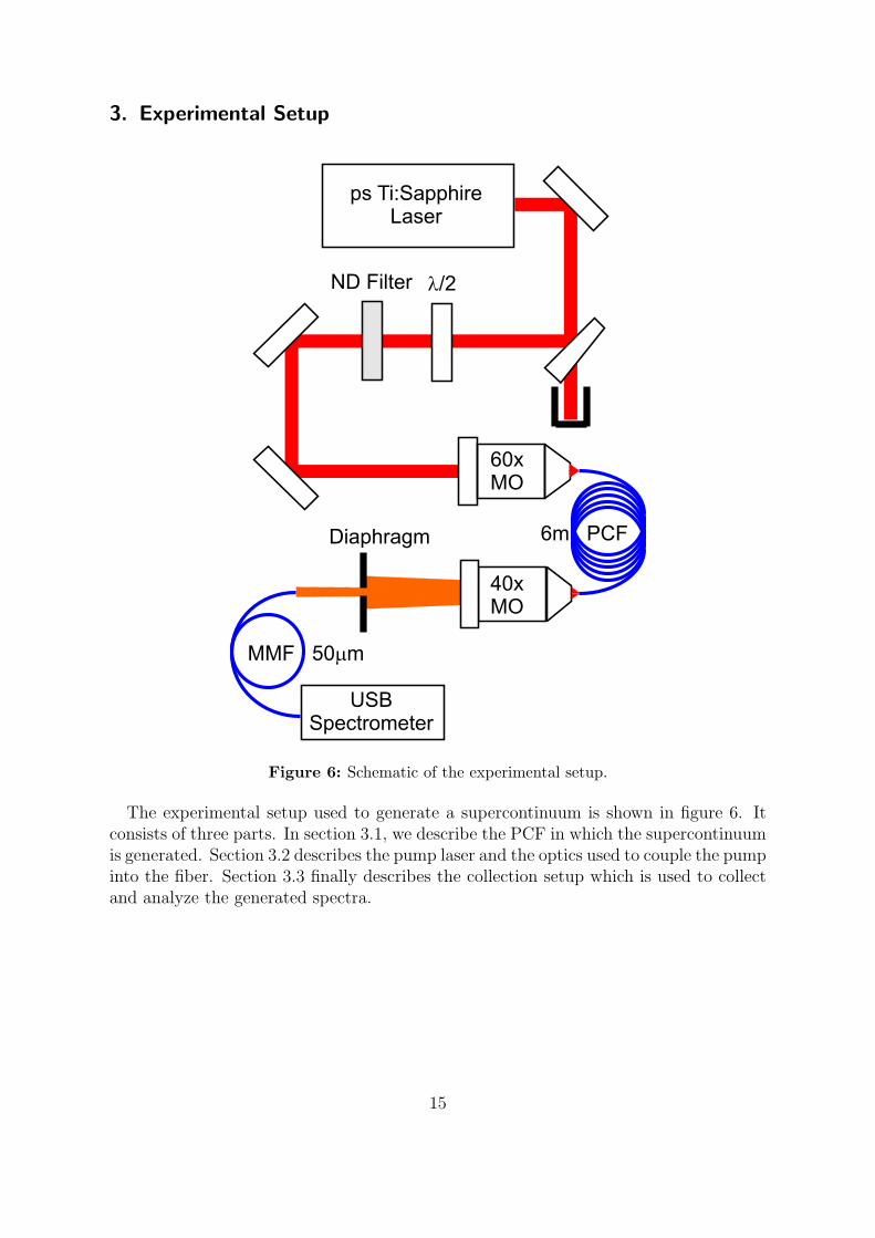
Figure 6: Schematic of the experimental setup.

The experimental setup used to generate a supercontinuum is shown in figure 6. Itconsists of three parts. In section 3.1, we describe the PCF in which the supercontinuumis generated. Section 3.2 describes the pump laser and the optics used to couple the pumpinto the fiber. Section 3.3 finally describes the collection setup which is used to collectand analyze the generated spectra.

15

3.1. Fiber Parameters

The single-mode step-index photonic crystal fiber used is the NL-PM-750 with a fiberlength of 6m, manufactured by Crystal Fibre. It has the following properties [4]:

• two zero-dispersion wavelengths, one at 750± 15 nm and one at 1260± 20 nm (seesection 2.3).

• an effective core diameter of 1.6± 0.3µm at 780 nm, related to the effective corearea.

• a nonlinear coefficient of γ =∼95 (Wkm)−1 at 780 nm (see sections 2.4.1 and 2.4.3).

• a cutoff wavelength λc ≤ 650 nm for multi-mode operation (see section 2.1)

• a numerical aperture of 0.38± 0.05 at 780 nm.

• an attenuation < 0.05 dB/m at 780 nm

• a birefringence of ∆n >3·10−4 (see section 2.1).

3.2. Pump Setup

The PCF is pumped by a picosecond mode-locked Ti:sapphire laser,7 pumped by a 7W532 nm CW diode laser.8 The wavelength can be tuned in the range between 700 and1000 nm, while the average power varies from 250mW at 1050 nm to 1.5W at 790 nm( [15], p. 3-13). The laser has a repetition rate of 82 MHz, a beam diameter of ∼2mmand the laser output is linearly polarized.

The average laser power of ∼1W was reduced to ∼100mW by reflecting the beamon a glass wedge under a 45o angle. The intensity was further controlled by a set ofneutral density (ND) filters. The polarization of the input beam is controlled witha λ/2 waveplate. The pump beam is coupled into the fiber using a 60x microscopeobjective9 (60xMO) on a XYZ stage. The 60xMO has an anti-reflection coating forvisible wavelengths and reflects a certain amount of light for wavelengths above 800 nm.These back reflections can interfere with mode-locking inside the laser cavity. This isavoided by slightly misaligning the beam and using filters to reduce the reflections (at836 nm in particular).

The average power coupled into the fiber (ACP) is determined by measuring the opti-cal power at the output facet of the fiber with a thermal photodetector. The measuredpower typically has a standard deviation of ∼0.2 mW. A coupling efficiency η - definedas ACP/input power - as high as 50% could be achieved. After a pump wavelengthis selected the spectrum of the laser is measured to determine this wavelength within0.2 nm accuracy. A stable pulse is found and the auto-correlator function is measured toget the pulse width within 0.1 ps accuracy. The beam is aligned such that the coupling

7Spectra Physics Tsunami8Spectra Physics Millenia X9Newport M-60X, NA = 0.85, f = 2.9 mm

16

efficiency is at least 30%.

-2 -1 0 1 2

Time (ps)

0.0

0.5

1.0

1.5

2.0

2.5

3.0

Ove

rlap

sign

al(V

)

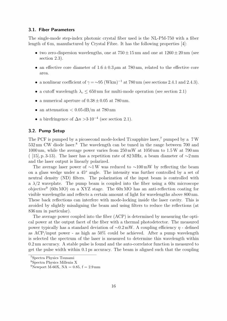
Figure 7: Auto-correlation function of a typical laser pulse. The time axis has been obtainedby the relation given in equation 3.1.

The pulse width of the laser pulse was measured using an auto-correlator setup. Inthis setup, the auto-correlator overlaps the pulse signal with a copy of itself inside aBBO crystal using a conventional interferometer setup, where second harmonic light isgenerated proportional to the measure of overlap. This overlap function can be describedas a convolution integral of two signals, see ( [10], pp. 539-543). Figure 7 gives a typicalauto-correlation function (acf). The FWHM of this acf is 2.0 ps.

The acf has been recorded on a digital oscilloscope using one of the outputs of theauto-correlator. This output monitors the second harmonic intensity while the auto-correlator moves one of its interferometer arms at a scanrate of 16,7Hz in a sinusoidalmotion over a distance expressed as the scanrange. The scanrange is 5 ps in this casewhich corresponds to a distance of 1.5mm; the amplitude x0 is then 0.75 mm.

The position of the interferometer arm as a function of time is given by: xacf =x0 sin(2πftacf ). At the same time we also know the distance travelled by the pulsewhich is the pulse time multiplied by the speed of light: xpulse = ctpulse. The two timescales are related by

tpulse =x0

csin(2πftacf ) (3.1)

The auto correlation function typically looks Gaussian, but the shape of the originalpulse is lost. You cannot deconvolute and hope to get it back, unless you have additionalinformation about your original pulse composition (in particular, phase information islost).

17

3.3. Collection and Analysis Setup

The generated supercontinuum is collected using a 40x MO10 at the exit of the fiber anda small fraction (∼(50µm/25mm)2 ≈ 2·10−6) using a pinhole is collected by a 50 µmcore multimode fiber (MMF) and sent to a spectrometer. All spectra are taken usingSpectraSuite software provided by Ocean Optics. The results are measured using 3 dif-ferent spectrometers (the USB4000, USB2000 and the NIR512) to cover the visible andinfrared range.

The spectrometers use a grating and spread the light of different wavelengths out overan array. This array is a linear silicon CCD array for the USB4000 and the USB2000and a InGaAs array for the NIR512. These detectors have a saturation level (related tothe pixel well depth of the array) which they were prevented from reaching by settingthe integration time by software. Spectra taken by the same spectrometer, but withdifferent integration times, are corrected for this difference so they can be compareddirectly.

The wavelength resolution for data from USB4000 spectrum analyzer varies from0.22 nm to 0.17 nm for wavelengths from respectively 178.14 nm to 886.96 nm (average0.195 nm). For the USB2000 resolution varies from 0.38 nm to 0.26 nm for wavelengthsfrom respectively 519.87 nm to 1172.85 nm (average 0.32 nm). For the NIR512 reso-lution varies from 1.72 nm to 1.67 nm for wavelengths from respectively 854.65 nm to1722.32 nm (average 1.695 nm).

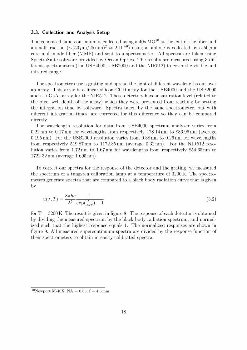
To correct our spectra for the response of the detector and the grating, we measuredthe spectrum of a tungsten calibration lamp at a temperature of 3200K. The spectro-meters generate spectra that are compared to a black body radiation curve that is givenby

u(λ, T ) =8πhc

λ5

1

exp( hcλkT

)− 1(3.2)

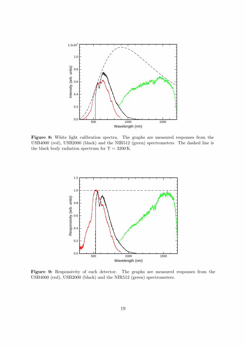
for T = 3200K. The result is given in figure 8. The response of each detector is obtainedby dividing the measured spectrum by the black body radiation spectrum, and normal-ized such that the highest response equals 1. The normalized responses are shown infigure 9. All measured supercontinuum spectra are divided by the response function oftheir spectrometers to obtain intensity-calibrated spectra.

10Newport M-40X, NA = 0.65, f = 4.5 mm.

18

500 1000 1500

Wavelength (nm)

0.0

0.2

0.4

0.6

0.8

1.0

1.2x104

Inte

nsity

(arb

.un

its)

Figure 8: White light calibration spectra. The graphs are measured responses from theUSB4000 (red), USB2000 (black) and the NIR512 (green) spectrometers. The dashed line isthe black body radiation spectrum for T = 3200K.

500 1000 1500

Wavelength (nm)

0.0

0.2

0.4

0.6

0.8

1.0

1.2

Res

pons

ivity

(arb

.un

its)

Figure 9: Responsivity of each detector. The graphs are measured responses from theUSB4000 (red), USB2000 (black) and the NIR512 (green) spectrometers.

19

4. Results

We start with the polarization dependence of the measured spectra in section 4.1, andcheck the influence of the birefringence on white light spectra. The pump wavelengthdependence is covered in section 4.2, to identify different regimes of dispersion. Finally,in section 4.3 the details of supercontinuum generation are studied by investigating thepower dependence at a constant pump wavelength.

4.1. Polarization Dependence

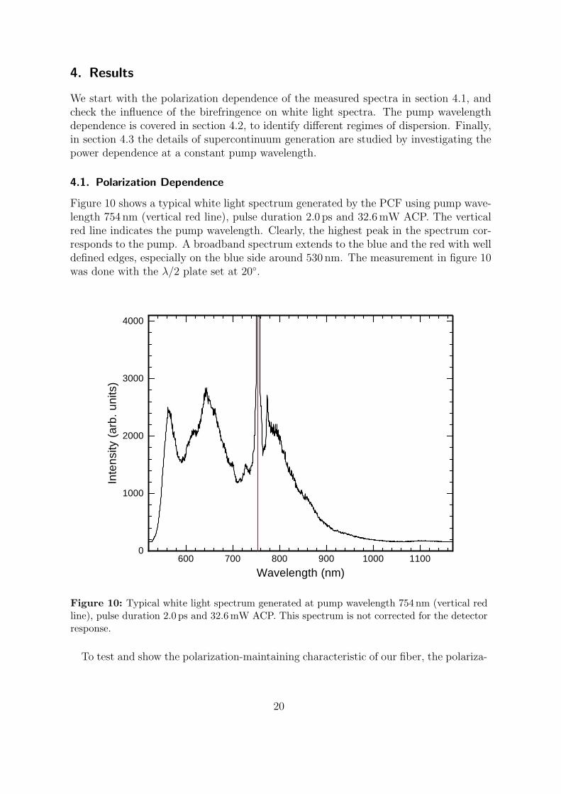
Figure 10 shows a typical white light spectrum generated by the PCF using pump wave-length 754 nm (vertical red line), pulse duration 2.0 ps and 32.6mW ACP. The verticalred line indicates the pump wavelength. Clearly, the highest peak in the spectrum cor-responds to the pump. A broadband spectrum extends to the blue and the red with welldefined edges, especially on the blue side around 530 nm. The measurement in figure 10was done with the λ/2 plate set at 20.

600 700 800 900 1000 1100

Wavelength (nm)

0

1000

2000

3000

4000

Inte

nsity

(arb

.un

its)

Figure 10: Typical white light spectrum generated at pump wavelength 754 nm (vertical redline), pulse duration 2.0 ps and 32.6 mW ACP. This spectrum is not corrected for the detectorresponse.

To test and show the polarization-maintaining characteristic of our fiber, the polariza-

20

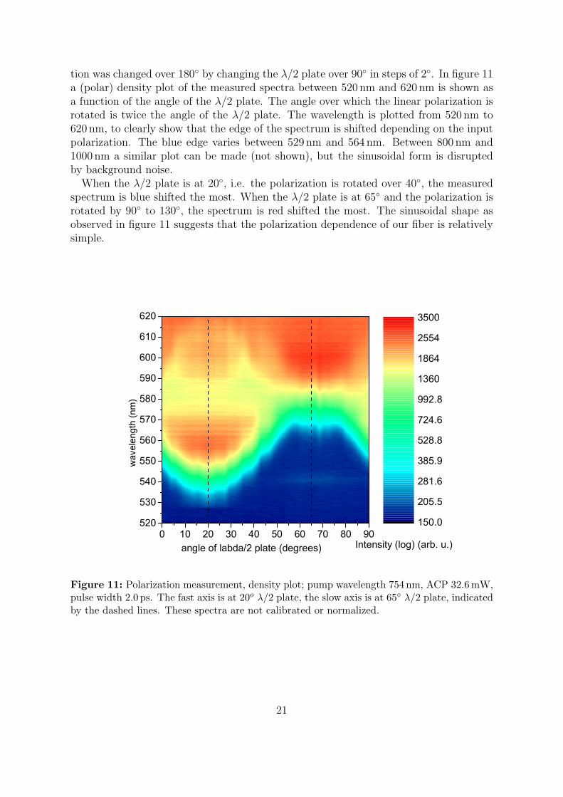
tion was changed over 180 by changing the λ/2 plate over 90 in steps of 2. In figure 11a (polar) density plot of the measured spectra between 520 nm and 620 nm is shown asa function of the angle of the λ/2 plate. The angle over which the linear polarization isrotated is twice the angle of the λ/2 plate. The wavelength is plotted from 520 nm to620 nm, to clearly show that the edge of the spectrum is shifted depending on the inputpolarization. The blue edge varies between 529 nm and 564 nm. Between 800 nm and1000 nm a similar plot can be made (not shown), but the sinusoidal form is disruptedby background noise.

When the λ/2 plate is at 20, i.e. the polarization is rotated over 40, the measuredspectrum is blue shifted the most. When the λ/2 plate is at 65 and the polarization isrotated by 90 to 130, the spectrum is red shifted the most. The sinusoidal shape asobserved in figure 11 suggests that the polarization dependence of our fiber is relativelysimple.

Figure 11: Polarization measurement, density plot; pump wavelength 754 nm, ACP 32.6 mW,pulse width 2.0 ps. The fast axis is at 20o λ/2 plate, the slow axis is at 65 λ/2 plate, indicatedby the dashed lines. These spectra are not calibrated or normalized.

21

4.2. Wavelength Dependence

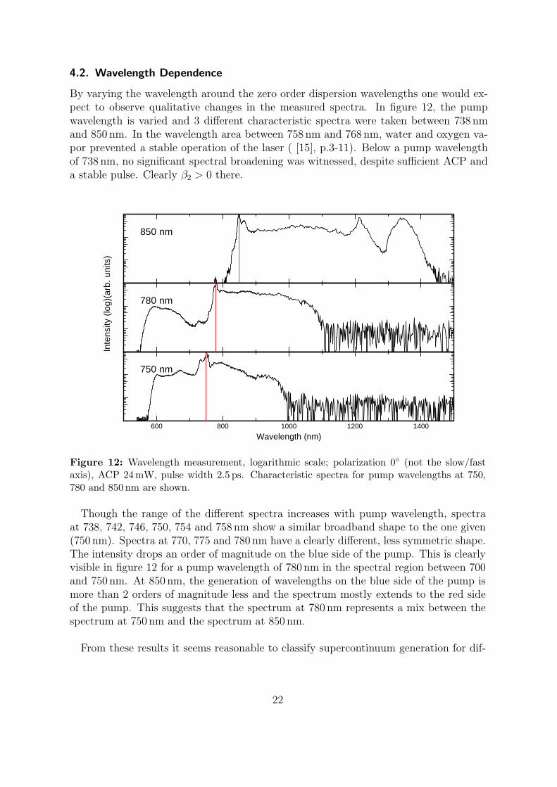
By varying the wavelength around the zero order dispersion wavelengths one would ex-pect to observe qualitative changes in the measured spectra. In figure 12, the pumpwavelength is varied and 3 different characteristic spectra were taken between 738 nmand 850 nm. In the wavelength area between 758 nm and 768 nm, water and oxygen va-por prevented a stable operation of the laser ( [15], p.3-11). Below a pump wavelengthof 738 nm, no significant spectral broadening was witnessed, despite sufficient ACP anda stable pulse. Clearly β2 > 0 there.

600 800 1000 1200 1400

Wavelength (nm)

Inte

nsity

(log)

(arb

.un

its)

750 nm

780 nm

850 nm

Figure 12: Wavelength measurement, logarithmic scale; polarization 0 (not the slow/fastaxis), ACP 24mW, pulse width 2.5 ps. Characteristic spectra for pump wavelengths at 750,780 and 850 nm are shown.

Though the range of the different spectra increases with pump wavelength, spectraat 738, 742, 746, 750, 754 and 758 nm show a similar broadband shape to the one given(750 nm). Spectra at 770, 775 and 780 nm have a clearly different, less symmetric shape.The intensity drops an order of magnitude on the blue side of the pump. This is clearlyvisible in figure 12 for a pump wavelength of 780 nm in the spectral region between 700and 750 nm. At 850 nm, the generation of wavelengths on the blue side of the pump ismore than 2 orders of magnitude less and the spectrum mostly extends to the red sideof the pump. This suggests that the spectrum at 780 nm represents a mix between thespectrum at 750 nm and the spectrum at 850 nm.

From these results it seems reasonable to classify supercontinuum generation for dif-

22

ferent pump wavelengths into two different regions, based on the dispersion curve:

• zero-dispersion, or close to it, β2 ≈ 0. Spectra with a pump wavelength ofbetween 738 and 758 nm fall in this category. The generated spectra are more orless symmetric and extend to the blue and the red of the pump wavelength.

• anomalous dispersion, β2 < 0. The generated spectra are strongly asymmetricand extend more to the red side of the pump than to the blue side. Spectra witha pump wavelength of 770 and higher exhibit this behavior.

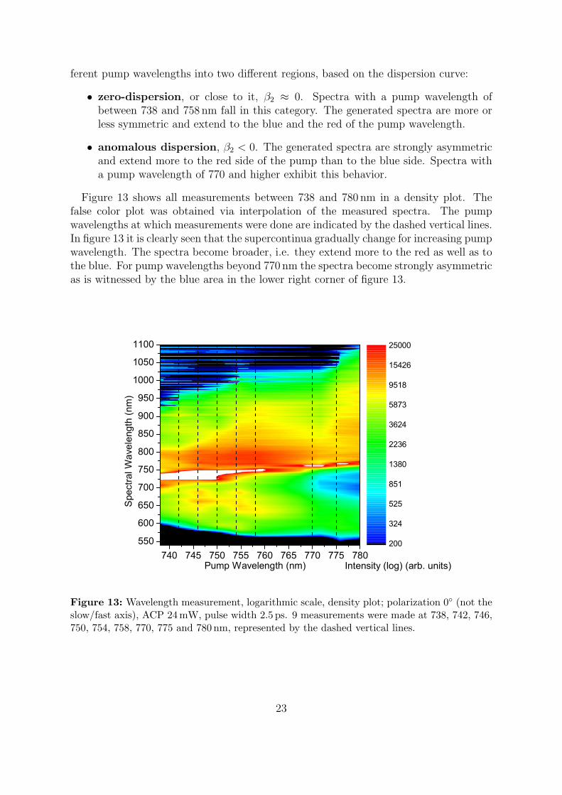
Figure 13 shows all measurements between 738 and 780 nm in a density plot. Thefalse color plot was obtained via interpolation of the measured spectra. The pumpwavelengths at which measurements were done are indicated by the dashed vertical lines.In figure 13 it is clearly seen that the supercontinua gradually change for increasing pumpwavelength. The spectra become broader, i.e. they extend more to the red as well as tothe blue. For pump wavelengths beyond 770 nm the spectra become strongly asymmetricas is witnessed by the blue area in the lower right corner of figure 13.

Figure 13: Wavelength measurement, logarithmic scale, density plot; polarization 0 (not theslow/fast axis), ACP 24 mW, pulse width 2.5 ps. 9 measurements were made at 738, 742, 746,750, 754, 758, 770, 775 and 780 nm, represented by the dashed vertical lines.

23

Wavelength dependence on the blue side of the pump in the anomalousdispersion regime

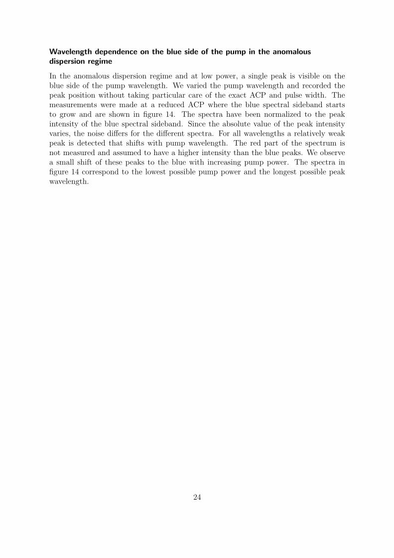
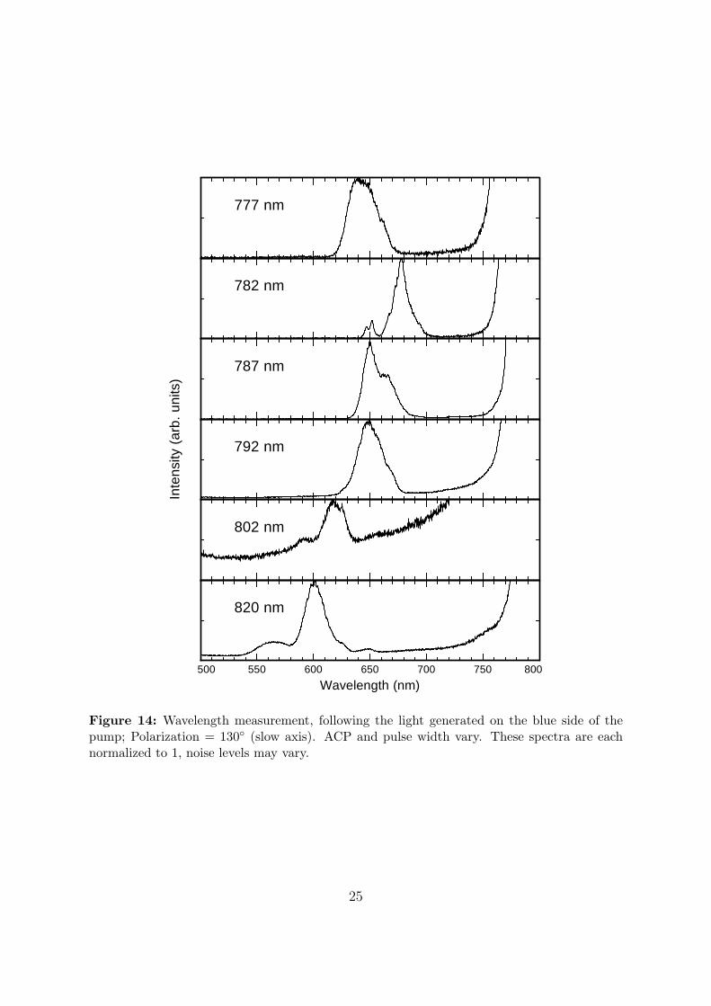
In the anomalous dispersion regime and at low power, a single peak is visible on theblue side of the pump wavelength. We varied the pump wavelength and recorded thepeak position without taking particular care of the exact ACP and pulse width. Themeasurements were made at a reduced ACP where the blue spectral sideband startsto grow and are shown in figure 14. The spectra have been normalized to the peakintensity of the blue spectral sideband. Since the absolute value of the peak intensityvaries, the noise differs for the different spectra. For all wavelengths a relatively weakpeak is detected that shifts with pump wavelength. The red part of the spectrum isnot measured and assumed to have a higher intensity than the blue peaks. We observea small shift of these peaks to the blue with increasing pump power. The spectra infigure 14 correspond to the lowest possible pump power and the longest possible peakwavelength.

24

500 550 600 650 700 750 800

Wavelength (nm)

Inte

nsity

(arb

.un

its)

777 nm

782 nm

787 nm

792 nm

802 nm

820 nm

Figure 14: Wavelength measurement, following the light generated on the blue side of thepump; Polarization = 130 (slow axis). ACP and pulse width vary. These spectra are eachnormalized to 1, noise levels may vary.

25

4.3. Power Dependence

In this section we study the influence of the average coupled power (ACP) on the gen-erated supercontinuum spectra in both the zero-dispersion and anomalous dispersionregimes. Decreasing ACP to below a value between 1 to 2mW typically gives a spec-trum with a single peak at the pump wavelength. By increasing the pump power (ACP),we can follow the supercontinuum generation and hopefully get some hints about theunderlying nonlinear processes.

4.3.1. Zero-Dispersion Regime

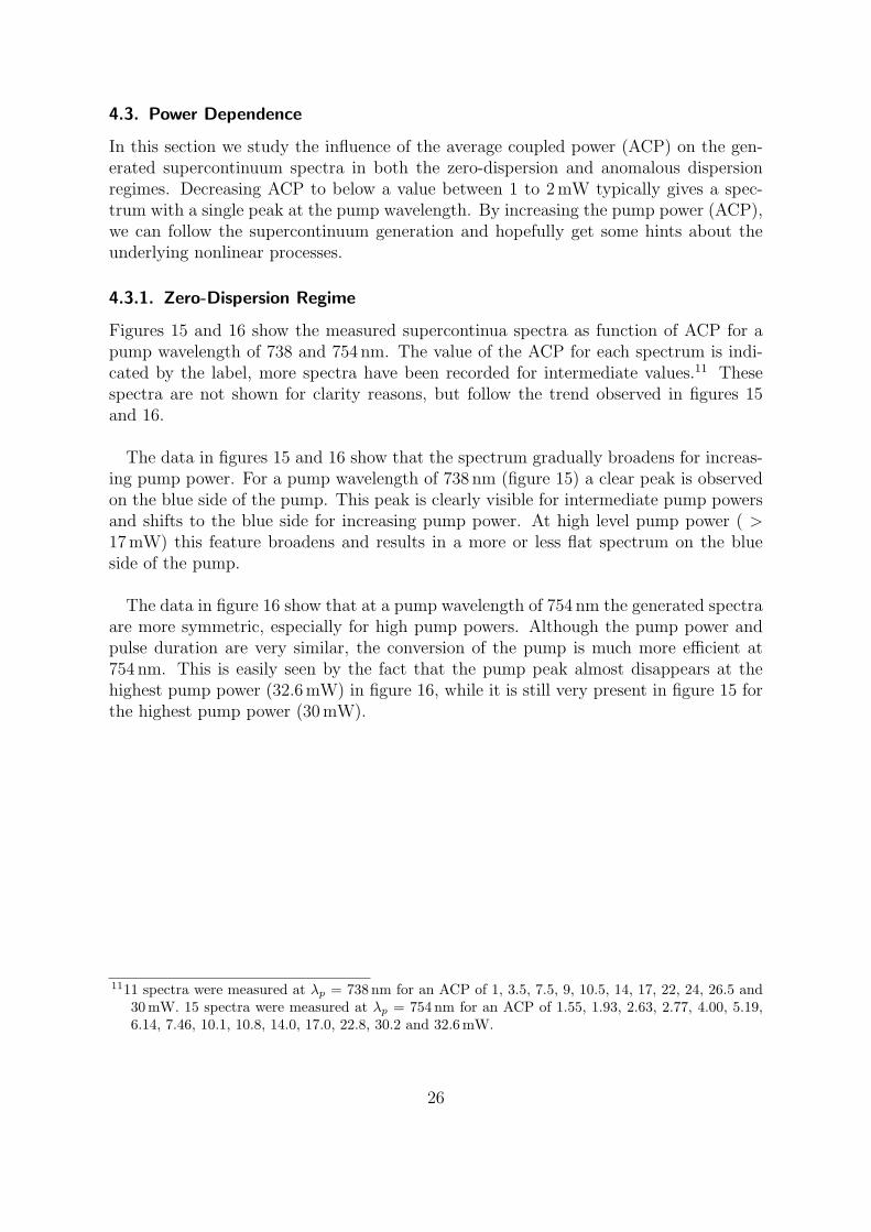
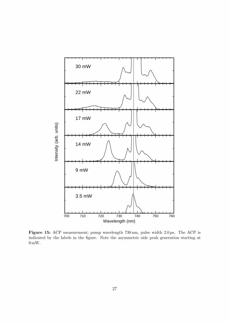
Figures 15 and 16 show the measured supercontinua spectra as function of ACP for apump wavelength of 738 and 754 nm. The value of the ACP for each spectrum is indi-cated by the label, more spectra have been recorded for intermediate values.11 Thesespectra are not shown for clarity reasons, but follow the trend observed in figures 15and 16.

The data in figures 15 and 16 show that the spectrum gradually broadens for increas-ing pump power. For a pump wavelength of 738 nm (figure 15) a clear peak is observedon the blue side of the pump. This peak is clearly visible for intermediate pump powersand shifts to the blue side for increasing pump power. At high level pump power ( >17mW) this feature broadens and results in a more or less flat spectrum on the blueside of the pump.

The data in figure 16 show that at a pump wavelength of 754 nm the generated spectraare more symmetric, especially for high pump powers. Although the pump power andpulse duration are very similar, the conversion of the pump is much more efficient at754 nm. This is easily seen by the fact that the pump peak almost disappears at thehighest pump power (32.6mW) in figure 16, while it is still very present in figure 15 forthe highest pump power (30mW).

1111 spectra were measured at λp = 738 nm for an ACP of 1, 3.5, 7.5, 9, 10.5, 14, 17, 22, 24, 26.5 and30mW. 15 spectra were measured at λp = 754 nm for an ACP of 1.55, 1.93, 2.63, 2.77, 4.00, 5.19,6.14, 7.46, 10.1, 10.8, 14.0, 17.0, 22.8, 30.2 and 32.6 mW.

26

700 710 720 730 740 750 760

Wavelength (nm)

Inte

nsity

(arb

.un

its)

3.5 mW

9 mW

14 mW

17 mW

22 mW

30 mW

Figure 15: ACP measurement; pump wavelength 738 nm, pulse width 2.0 ps. The ACP isindicated by the labels in the figure. Note the asymmetric side peak generation starting at9mW.

27

600 700 800 900 1000

Wavelength (nm)

Inte

nsity

(arb

.un

its)

2.6 mW

5.2 mW

10.1 mW

17 mW

32.6 mW

Figure 16: ACP measurement; pump wavelength 754 nm, pulse 2.0 ps. The ACP is indicatedby the labels in the figure. On the red side of the pump intensities are higher than on the blueside, for an ACP up to 22mW. At the highest ACP the spectrum becomes more symmetric.

28

4.3.2. Anomalous Dispersion Regime

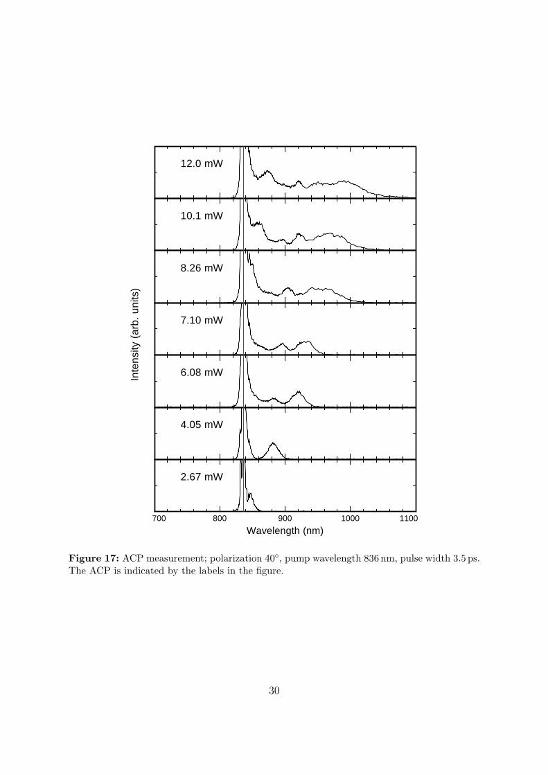
Figure 17 shows the measured power dependence in the anomalous regime at a pumpwavelength of 836 nm (figure 17). The asymmetry of the spectra is striking. No super-continuum was generated at the blue side of the pump for pump powers up to 12mW.Higher pump powers are not possible at this pump wavelength because reflections fromthe microscope objective disturb the mode-locked operation of the laser (see section 3.2).

Especially at the lower pump powers a clear Gaussian shaped peak is visible at the redside of the pump. The peak continuously shifts to the red with increasing pump power.The frequency shift with increasing ACP as observed in figure 17 can be quantified.For the first four spectra (up to 7.10mW) the peak position of the longest wavelengthpeak is noted. For higher ACP, a gaussian shape is loosely drawn through the longestwavelength peak and its center position (λS) is noted.

Figure 18 shows the frequency shift ∆ω2 = (ωS − ωp)2 as a function of ACP. Notethat we plot the square of the frequency shift. A straight line in figure 18 thus givesa shift that increases linearly with the field amplitude (given by the square root of theACP). Our experimental data is best described by such a dependence and the best fit tothe data (red line in figure 18) gives a slope of 1.33 ± 0.05 1028Hz2mW−1 and an offsetof -3.64 ± 0.38 1028 Hz2. This offset on the vertical axis corresponds to an ACP of 2.74± 0.27mW below which no shift is observed, called a threshold. Similar linear relationshave been found for pump wavelengths at 850 nm and 754 nm. For those wavelengthsthere are fewer data points at low pump powers and it is more difficult to establish athreshold as observed in figure 18.

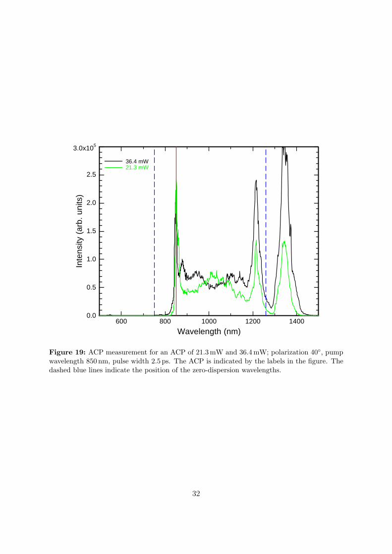
At 850 nm we were able to reach larger values of ACP. The recorded spectra resemblethose for 836 nm pump wavelength and are strongly asymmetric. The spectrum for anACP of 24mW is shown in figure 12 (top) and extends to ∼1400 nm. Spectra for anACP of 21.3 and 36.4mW are shown in figure 19 over a wavelength range from 500 to1500 nm. For these values of the pump power the spectrum does not extend further tothe red beyond 1400 nm; the red sideband peaks around 1215 and 1345 nm do not shiftwith increasing pump power. The structure in the spectral range between the pump(850 nm) and the first peak (1215 nm) do change with increasing ACP. A clear dip inthe intensity is visible in between the two peaks around 1285 nm.

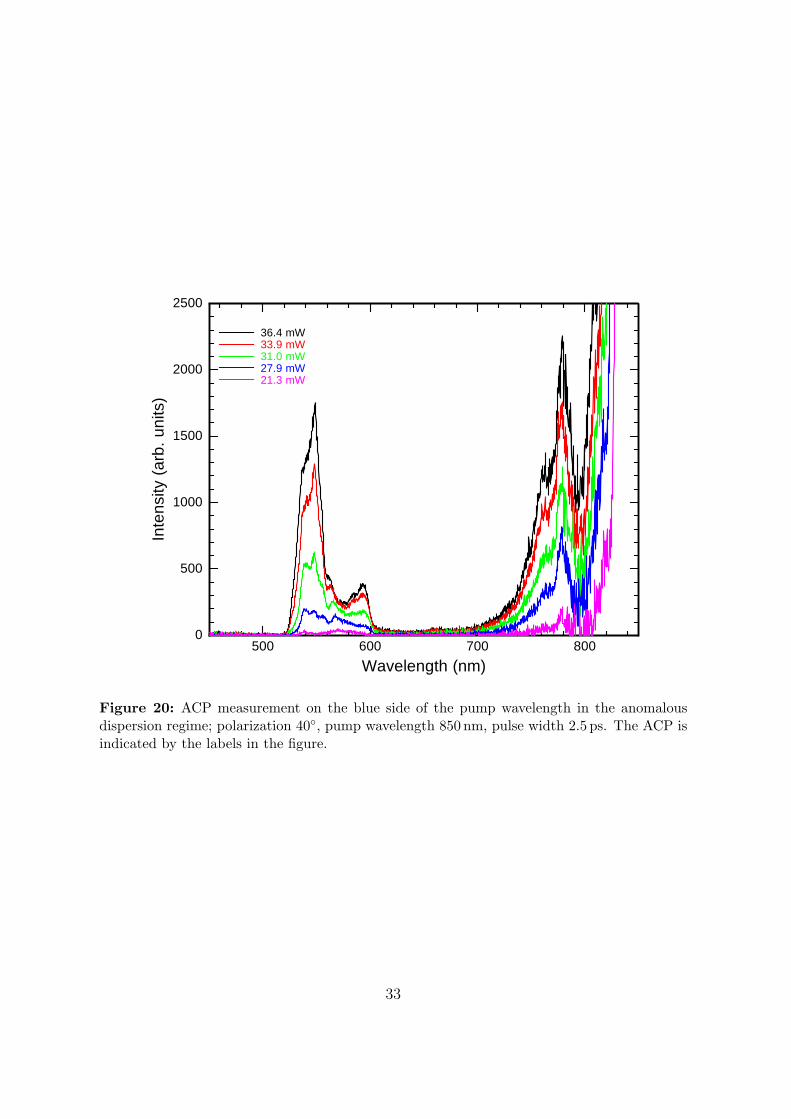
Close inspection of the blue side of the spectrum reveals a small peaks around ∼550 nmand ∼780 nm. These blue sideband peaks are shown in more detail in figure 20 for dif-ferent values of the ACP. Additional measurements were done at an ACP of 24.1, 29.1,33.0 and 35.4 mW (not shown). The peaks grow in intensity with increasing ACP, butdo not shift. At these high pump powers, the fiber lights up more or less uniformly witha green to yellow color.

29

700 800 900 1000 1100

Wavelength (nm)

Inte

nsity

(arb

.un

its)

2.67 mW

4.05 mW

6.08 mW

7.10 mW

8.26 mW

10.1 mW

12.0 mW

Figure 17: ACP measurement; polarization 40, pump wavelength 836 nm, pulse width 3.5 ps.The ACP is indicated by the labels in the figure.

30

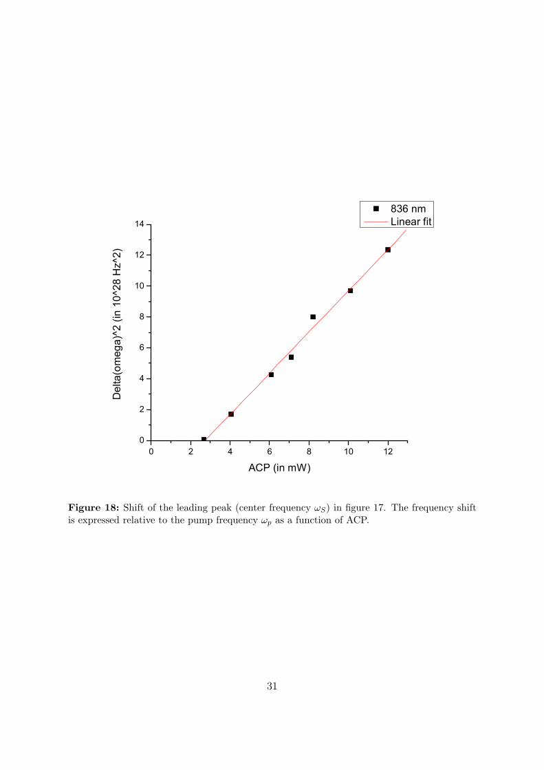
Figure 18: Shift of the leading peak (center frequency ωS) in figure 17. The frequency shiftis expressed relative to the pump frequency ωp as a function of ACP.

31

600 800 1000 1200 1400

Wavelength (nm)

0.0

0.5

1.0

1.5

2.0

2.5

3.0x105

Inte

nsity

(arb

.un

its)

36.4 mW21.3 mW

Figure 19: ACP measurement for an ACP of 21.3mW and 36.4 mW; polarization 40, pumpwavelength 850 nm, pulse width 2.5 ps. The ACP is indicated by the labels in the figure. Thedashed blue lines indicate the position of the zero-dispersion wavelengths.

32

500 600 700 800

Wavelength (nm)

0

500

1000

1500

2000

2500

Inte

nsity

(arb

.un

its)

36.4 mW33.9 mW31.0 mW27.9 mW21.3 mW

Figure 20: ACP measurement on the blue side of the pump wavelength in the anomalousdispersion regime; polarization 40, pump wavelength 850 nm, pulse width 2.5 ps. The ACP isindicated by the labels in the figure.

33

5. Discussion

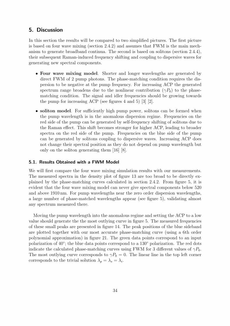
In this section the results will be compared to two simplified pictures. The first pictureis based on four wave mixing (section 2.4.2) and assumes that FWM is the main mech-anism to generate broadband continua. The second is based on solitons (section 2.4.4),their subsequent Raman-induced frequency shifting and coupling to dispersive waves forgenerating new spectral components.

• Four wave mixing model. Shorter and longer wavelengths are generated bydirect FWM of 2 pump photons. The phase-matching condition requires the dis-persion to be negative at the pump frequency. For increasing ACP the generatedspectrum range broadens due to the nonlinear contribution (γP0) to the phase-matching condition. The signal and idler frequencies should be growing towardsthe pump for increasing ACP (see figures 4 and 5) [3] [2].

• soliton model. For sufficiently high pump power, solitons can be formed whenthe pump wavelength is in the anomalous dispersion regime. Frequencies on thered side of the pump can be generated by self-frequency shifting of solitons due tothe Raman effect. This shift becomes stronger for higher ACP, leading to broaderspectra on the red side of the pump. Frequencies on the blue side of the pumpcan be generated by solitons coupling to dispersive waves. Increasing ACP doesnot change their spectral position as they do not depend on pump wavelength butonly on the soliton generating them [16] [8].

5.1. Results Obtained with a FWM Model

We will first compare the four wave mixing simulation results with our measurements.The measured spectra in the density plot of figure 13 are too broad to be directly ex-plained by the phase-matching curves calculated in section 2.4.2. From figure 5, it isevident that the four wave mixing model can never give spectral components below 520and above 1910 nm. For pump wavelengths near the zero order dispersion wavelengths,a large number of phase-matched wavelengths appear (see figure 5), validating almostany spectrum measured there.

Moving the pump wavelength into the anomalous regime and setting the ACP to a lowvalue should generate the the most outlying curve in figure 5. The measured frequenciesof these small peaks are presented in figure 14. The peak positions of the blue sidebandare plotted together with our most accurate phase-matching curve (using a 6th orderpolynomial approximation) in figure 21. The green data points correspond to an inputpolarization of 40; the blue data points correspond to a 130 polarization. The red dotsindicate the calculated phase-matching curves using FWM for 3 different values of γP0.The most outlying curve corresponds to γP0 = 0. The linear line in the top left cornercorresponds to the trivial solution λp = λs = λi.

34

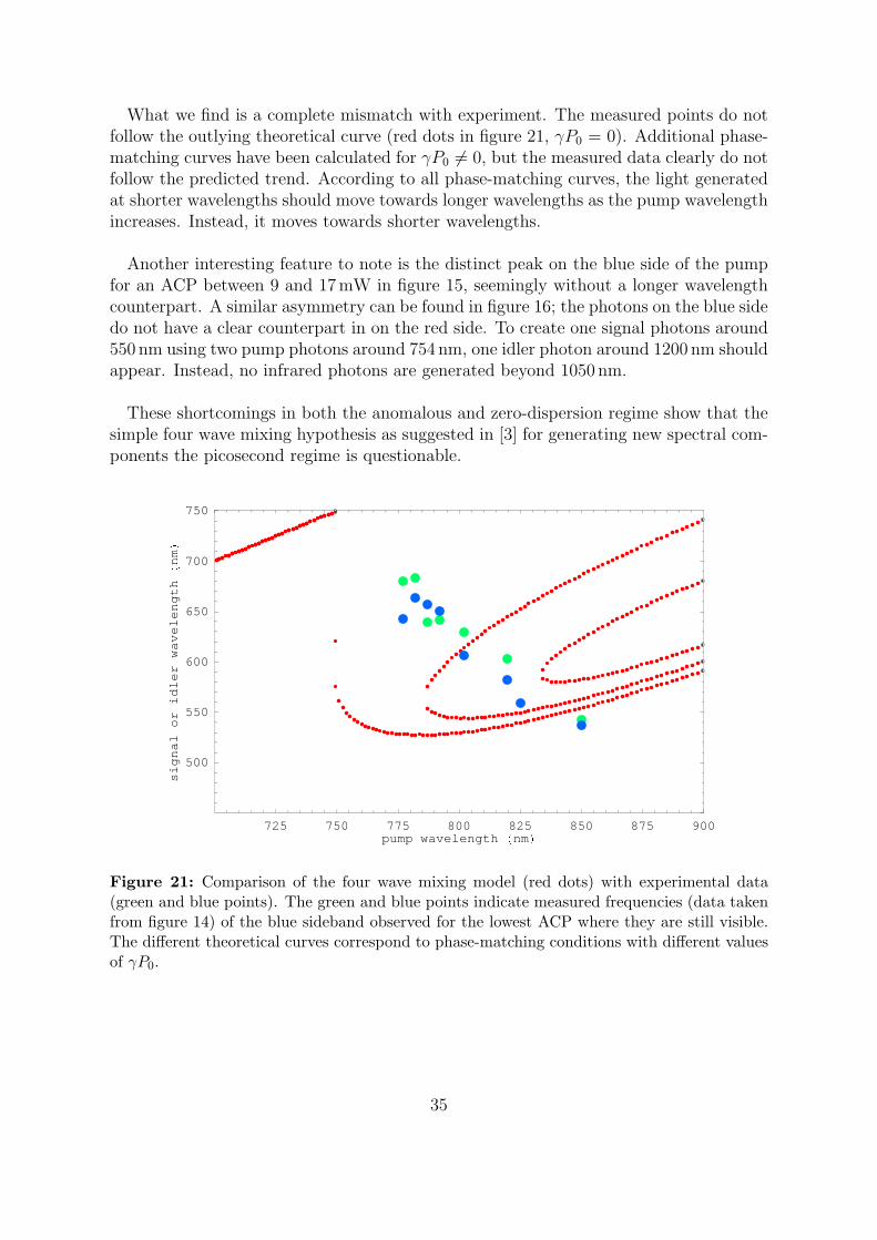
What we find is a complete mismatch with experiment. The measured points do notfollow the outlying theoretical curve (red dots in figure 21, γP0 = 0). Additional phase-matching curves have been calculated for γP0 6= 0, but the measured data clearly do notfollow the predicted trend. According to all phase-matching curves, the light generatedat shorter wavelengths should move towards longer wavelengths as the pump wavelengthincreases. Instead, it moves towards shorter wavelengths.

Another interesting feature to note is the distinct peak on the blue side of the pumpfor an ACP between 9 and 17mW in figure 15, seemingly without a longer wavelengthcounterpart. A similar asymmetry can be found in figure 16; the photons on the blue sidedo not have a clear counterpart in on the red side. To create one signal photons around550 nm using two pump photons around 754 nm, one idler photon around 1200 nm shouldappear. Instead, no infrared photons are generated beyond 1050 nm.

These shortcomings in both the anomalous and zero-dispersion regime show that thesimple four wave mixing hypothesis as suggested in [3] for generating new spectral com-ponents the picosecond regime is questionable.

725 750 775 800 825 850 875 900pump wavelength

nm

500

550

600

650

700

750

la

ng

is

ro

re

ld

ih

tg

ne

le

va

w

mn

Figure 21: Comparison of the four wave mixing model (red dots) with experimental data(green and blue points). The green and blue points indicate measured frequencies (data takenfrom figure 14) of the blue sideband observed for the lowest ACP where they are still visible.The different theoretical curves correspond to phase-matching conditions with different valuesof γP0.

35

5.2. Results Obtained with a Soliton Model

The soliton hypothesis finds its validation more through describing and understandingthe generation of broadband spectra than through calculations, since solving the NLSEis difficult, lengthy and numerical. The frequency shift observed in figure 17 and thelinear relation in figure 18 are consistent with observations and calculations made byothers [17] [18].

A clear threshold is found in figure 18. The data in the anomalous regime (sec-tion 4.3.2) can be understood qualitatively as follows: Below a certain threshold powerno solitons are formed and no frequency shifting occurs. Above the threshold a solitonforms. The Raman effect causes a frequency shift of the soliton that scales with thesquare root of the pump power [19] [16].

The relatively weak peaks on the blue side of the pump in figures 20 and 19 might beexplained if the solitons couple to dispersive waves [8]. This coupling to dispersive wavesdoes not depend on the wavelength of the pump but on the wavelength of the solitongenerating them (see equation 2.28). If the soliton no longer frequency shifts because itreaches the second zero-dispersion wavelength, the phase-matching condition to createthe dispersive waves would not change. This would explain why the peaks on the blueand red sides do not shift with pump power.

The intensity of wavelengths generated on the blue side of the pump decreases twoorders of magnitude as the pump wavelength is moved into the anomalous dispersionregime (see figure 12) from 750 to 850 nm. This corresponds to a decrease of β2 equalto -180 fs2cm−1. Apparently, the generation of blue light is very inefficient when β2 isstrongly negative. When the wavelength of the pump is tuned towards lower values of|β2|, the generation of blue light becomes more efficient. This might be explained bythe phase-matching condition for the coupling of dispersive wave to the soliton (equa-tion 2.28). It would be desirable to evaluate this phase-matching condition in order toconfirm that the blue light is indeed due to dispersive waves.

Close to the normal dispersion regime (β2 > 0), a clear peak that shifts to the bluewith increasing pump power is observed, see figure 15. Both the frequency shift as wellas the Gaussian shape of the peak are remarkably similar to what is observed at a pumpwavelength of 836 nm. The only difference being that the peak shifts to the blue andthat it flattens out for higher pump powers. Clearly, the peak cannot be interpreted asa soliton, as solitons do not exist in the normal dispersion regime, nor do they flattenout (they split to lower-order solitons). We speculate that the peak on the blue side ofthe pump is still caused by dispersive waves from a soliton that exists in the anomalousdispersion regime. With increasing pump power, the phase-matching condition wouldchange. Again, to quantitatively support this hypothesis a numerical solution of thephase-matching condition (equation 2.28) is necessary.

36

6. Conclusion

We have studied supercontinua generated with picosecond pulses in a 6m long photoniccrystal fiber (NL-750-PM, [4]). The supercontinuum that can be generated stronglydepends on the pump wavelength and the peak power. We have varied the pump wave-length between 738 to 850 nm and the average coupled power (ACP) between 2 to 32mW.No supercontinuum can be generated for pump wavelengths below 738 nm. Between 738and 758 nm supercontinua are found that extend to the blue as well as to the red side ofthe pump. For pump wavelengths of 770 nm and longer, the measured spectra extendmostly to the red.

Our measured cannot be explained by a simple four wave mixing model. The measuredspectra lack the symmetry expected, especially when the pump wavelength is tuned tothe anomalous dispersion regime. Even in the zero-dispersion regime, the predictedStokes bands are found missing. Therefore we conclude that direct four wave mixing ofthe pump to create new wavelengths is not important.

Instead our measurements strongly suggest that solitons are responsible for the ob-served features in the spectra. For pump wavelengths around 850 nm, the spectra extendmostly to the red and show a frequency shift that is linear with the amplitude of thepulse. Qualitatively this can be understood in terms of a self-frequency shift of thesolitons due to the Raman effect. Within the same model, blue spectral components canbe generated by coupling of the soliton to dispersive waves. To get a good quantitativeagreement and to confirm this hypothesis one is required to numerically solve the phase-matching condition for dispersive waves and/or the nonlinear Schrodinger equation.

Acknowledgement

I would like to thank the following people:

• Michiel de Dood for his excellent supervision, his useful advices and especially hispatience when explaining things more than once.

• Eduard Driessen for his useful advices and particular experimental insight.

• The Quantum Optics and Information group for their support, all the discussionsand conversations at the coffee table.

37

References

[1] Kim P. Hansen and Rene E. Kristiansen. ”Supercontinuum Generation inPhotonic Crystal Fibers”, www.crystal-fibre.com

[2] Thomas V. Andersen et al. ”Continuous-wave wavelength conversion ina photonic crystal fiber with two zero-dispersion wavelengths”, OpticsExpress, 2004, vol. 12, no. 17, pp. 4113-4122.

[3] Karen Marie Hilligsøe, et al. ”Supercontinuum generation in a photoniccrystal fiber with two zero-dispersion wavelengths”, Optics Express, 2004,vol. 12, no. 6, pp. 1045-1054.

[4] http://www.crystal-fibre.com/datasheets/NL-PM-750.pdf

[5] http://en.wikipedia.org/wiki/Self-phase modulation

[6] Masanori Koshiba and Kunimasa Saitoh. ”Applicability of classical opticalfiber theories to holey fibers”, Optics Letters, 2004, vol. 29, no. 15, pp.1739-1741.

[7] Niels Asger Mortensen and Jacob Riis Folkenberg, ”Modal cutoff and theV parameter in photonic crystal fibers”, Optics Letters, 2003, vol. 28, no.20, pp. 1879-1881.

[8] A. V. Husakou and J. Herrmann. ”Supercontinuum generation of higher-order solitons by fission in photonic crystal fibers”, Phys. Rev. Letters,2001, vol. 87, no. 20, pp. 203901-1 to -3.

[9] http://www.tpub.com/neets/tm/109-4.htm

[10] Eugene Hecht, 1998. Optics, 3rd ed., Addison-Wesley, MA.

[11] Govind P. Agrawal, 2001. Nonlinear Fiber Optics, 3rd ed., AcademicPress, CA.

[12] Allan W. Snyder and John D. Love, 1983. Optical Waveguide Theory,Kluwer Academic Publishers, Dordrecht, Netherlands.

[13] http://en.wikipedia.org/wiki/Self-phase modulation

[14] Robert W. Boyd, 1992. Nonlinear Optics, Academic Press, CA.

[15] Spectra Physics, 2002. Tsunami, User’s Manual.

[16] J. Herrmann, et al. ”Experimental evidence for supercontinuum gener-ation by fission of higher-order solitons in photonic fibers”, Phys. Rev.Letters, 2002, vol. 88, no. 17, pp. 173901-1 to -4.

38

[17] M. G. Banaee and Jeff F. Young. ”High-order soliton breakup and solitonself-frequency shifts in a microstructured optical fiber”, J. Opt. Soc. Am.B, 2006, vol. 23, no. 7, pp. 1484-1489.

[18] J. K. Lucek and K. J. Blow. ”Soliton self-frequency shift in telecommuni-cations fiber”, Phys. Rev. A, 1992, vol. 45, no. 9, pp. 6666-6674.

[19] P. K. A. Wai, et al. ”Soliton at the zero-group-dispersion wavelength of asingle-model fiber”, Optics Letters, 1987, vol. 12, no. 8, pp. 628-630.

39

A. Tables

Table 1: Values taken from the dispersion curve in figure 2, used for fitting. Values for ω arecalculated from λ.

λ (10−9 m) ω (1015 Hz) β2 (10−25s2m−1)

600 3.141593 0.3855650 2.899932 0.2264700 2.692794 0.1132750 2.513274 0800 2.356194 -0.1038850 2.217595 -0.1792900 2.094395 -0.2547950 1.984164 -0.32081000 1.884956 -0.36791050 1.795196 -0.38681100 1.713596 -0.36791150 1.639092 -0.31131200 1.570796 -0.18871250 1.507964 -0.37741300 1.449966 0.21691350 1.396263 0.5001400 1.346397 0.87741450 1.299969 1.32081500 1.256637 1.88731526 1.235065 2.1604

Table 2: Fitting parameters for 2nd and 6th order polynomial fits to β2 in section 2.4.2. ωshould be entered in units of 1015 Hz to give β2 in units of 10−25 s2m−1.

a + bω + cω2 a + bω + cω2 + dω3 + eω4 + fω5 + gω6

a = 8.59221 a = 238.319b = -8.1057 b = -603.905c = 1.8015 c = 633.827

d = -353.61e = 110.627f = -18.3883g = 1.26783

40