Sunayana Ghosh, Sylvain Petitjean, Gert Vegter To cite ... · Approximation by conic splines Sunayana Ghosh, ... among all such bitangent conics. ... Paper overview. Section 2 reviews

HAL Id: inria-00188456https://hal.inria.fr/inria-00188456

Submitted on 30 Jun 2011

HAL is a multi-disciplinary open accessarchive for the deposit and dissemination of sci-entific research documents, whether they are pub-lished or not. The documents may come fromteaching and research institutions in France orabroad, or from public or private research centers.

L’archive ouverte pluridisciplinaire HAL, estdestinée au dépôt et à la diffusion de documentsscientifiques de niveau recherche, publiés ou non,émanant des établissements d’enseignement et derecherche français ou étrangers, des laboratoirespublics ou privés.

Approximation by conic splinesSunayana Ghosh, Sylvain Petitjean, Gert Vegter

To cite this version:Sunayana Ghosh, Sylvain Petitjean, Gert Vegter. Approximation by conic splines. Mathematics inComputer Science, Springer, 2007, 1 (1), pp.39-69. <10.1007/s11786-007-0004-8>. <inria-00188456>

https://hal.inria.fr/inria-00188456

https://hal.archives-ouvertes.fr

APPROXIMATION BY CONIC SPLINES

SUNAYANA GHOSH, SYLVAIN PETITJEAN, AND GERT VEGTER

Abstract. We show that the complexity of a parabolic or conic spline approx-imating a sufficiently smooth curve with non-vanishing curvature to withinHausdorff distance ε is c1ε−1/4 + O(1), if the spline consists of parabolic arcs,

and c2ε−1/5 + O(1), if it is composed of general conic arcs of varying type.The constants c1 and c2 are expressed in the Euclidean and affine curvatureof the curve. We also show that the Hausdorff distance between a curve andan optimal conic arc tangent at its endpoints is increasing with its arc length,provided the affine curvature along the arc is monotone. This property yieldsa simple bisection algorithm for the computation of an optimal parabolic orconic spline.

1. Introduction

In the field of computer aided geometric design, one of the central topics is theapproximation of complex geometric objects with simpler ones. An important partof this field concerns the approximation of plane curves and the asymptotic anal-ysis of the rate of convergence of approximation schemes with respect to differentmetrics, the most commonly used being the Hausdorff metric.

Various error bounds and convergence rates have been obtained for several typesof (low-degree) approximation primitives. For the approximation of plane convexcurves by polygons with n edges, the order of convergence is O(n−2) for severalmetrics, including the Hausdorff metric [13, 16, 17, 19]. When approximating bya tangent continuous conic spline, the order of convergence, for a strictly convexcurve, is O(n−5), where n is the number of elements of the conic spline, with respectto the Hausdorff distance metric [26]. For the approximation of a convex curve bya piecewise cubic curve, both curves being tangent and having the same Euclideancurvature at interpolation points (knots), the order of approximation is O(h6),where h is the maximum distance between adjacent knots [5]. As expected, the ap-proximation order increases along with the degree of the approximating (piecewise-)polynomial curve.

As approximants, conic splines represent a good compromise between flexibilityand modeling power. They have a great potential as intermediate representationfor robust computation with curved objects. Some applications that come to mindare the implicitization of parametric curves (see works on approximate implicitiza-tion [8, 9]), the intersection of high-degree curves, the building of arrangements ofalgebraic curves (efficient solutions are known for sweeping arrangements of conicarcs [2]) and the computation of the Voronoi diagram of curved objects (the caseof ellipses has been recently investigated [10, 11]).

The research of SG and GV was partially supported by grant 6413 of the European Commissionto the IST-2002 FET-Open project Algorithms for Complex Shapes in the Sixth FrameworkProgram.

1

2 S. GHOSH, S. PETITJEAN, AND G. VEGTER

While these applications necessitate a tight hold on the error of approximation,no previous work provides a sharp asymptotic error bound (i.e., the constant ofthe leading term in the asymptotic expansion) for the Hausdorff metric when theinterpolant is curved.

In this paper, we study the optimal approximation of a sufficiently smooth curvewith non-vanishing curvature by a tangent continuous interpolating conic spline,which is an optimal approximant with respect to Hausdorff distance. We presentthe first sharp asymptotic bound on the approximation error (and, consequently, asharp bound on the complexity of the approximation) for both parabolic and conicinterpolating splines. Our experiments corroborate this sharp bound: the complex-ity of the approximating splines we algorithmically construct exactly matches thecomplexity predicted by our complexity bound.

1.1. Related work. Fejes Toth [13] considers the problem of approximating aconvex C2-curve C in the plane by an inscribed n-gon. Fejes Toth proves that,with regard to the Hausdorff distance, the optimal n-gon Pn satisfies

(1.1) δH(C,Pn) =1

8

(∫ l

0

κ1/2(s) ds

)21

n2+O

( 1

n4

)

.

Here δH(A,B) is the Hausdorff distance between two sets A and B, l is the lengthof the curve, s its arc length parameter, and κ(s) its curvature. An asymptotic ex-pression for the complexity of the piecewise linear spline can easily be deduced: the

number of elements is c ε−1/2 (1+O(ε)), where c = 12√

2

∫ l

s=0 κ(s)1/2 ds. Ludwig [17]

extends this result by deriving the second term in the asymptotic expansion (1.1).If one considers the symmetric difference metric δS instead, one can prove that

δS(C,Pn) = 112

(∫ l

0κ1/3(s)ds

)31

n2 +O( 1n4 ) [19]. Again, this asymptotic expression

can be refined, cf. [16].Schaback [26] introduces a scheme that yields an interpolating conic spline with

tangent continuity for a curve with non-vanishing curvature, and achieves an ap-proximation order of O(h5), where h is the maximal distance of adjacent datapoints on the curve. A conic spline consists of pieces of conics, in principle ofvarying type. This result implies that approximating such a curve by a curva-ture continuous conic spline to within Hausdorff distance ε requires O(ε−1/5) ele-ments. However, the value of the constant implicit in this asymptotic expressionof the complexity is not known. Ludwig [18] considers the problem of optimallyapproximating a convex C4-curve with respect to the symmetric difference met-ric by a tangent continuous parabolic spline Qn with n knots. She proves that

δS(C,Qn) = 1240

(∫ λ

0 κ1/5(s)ds

)51

n4 + o( 1n4 ), where λ =

∫ l

0 κ1/3(s)ds is the affine

length of the convex curve C.These problems fall in the context of geometric Hermite interpolation, in which

approximation problems for curves are treated independent of their specific pa-rameterization. The seminal paper by De Boor, Hollig and Sabin [5] fits in thiscontext. Floater [14] gives a method that, for any conic arc and any odd integer n,yields a geometric Hermite interpolant with 2n contacts, counted with multiplicity.This scheme gives a Gn−1-spline, and has approximation order O(h2n), where h isthe length of the conic arc. Ahn [1] gives a necessary and sufficient condition forthe conic section to be the optimal approximation of the given planar curve with

APPROXIMATION BY CONIC SPLINES 3

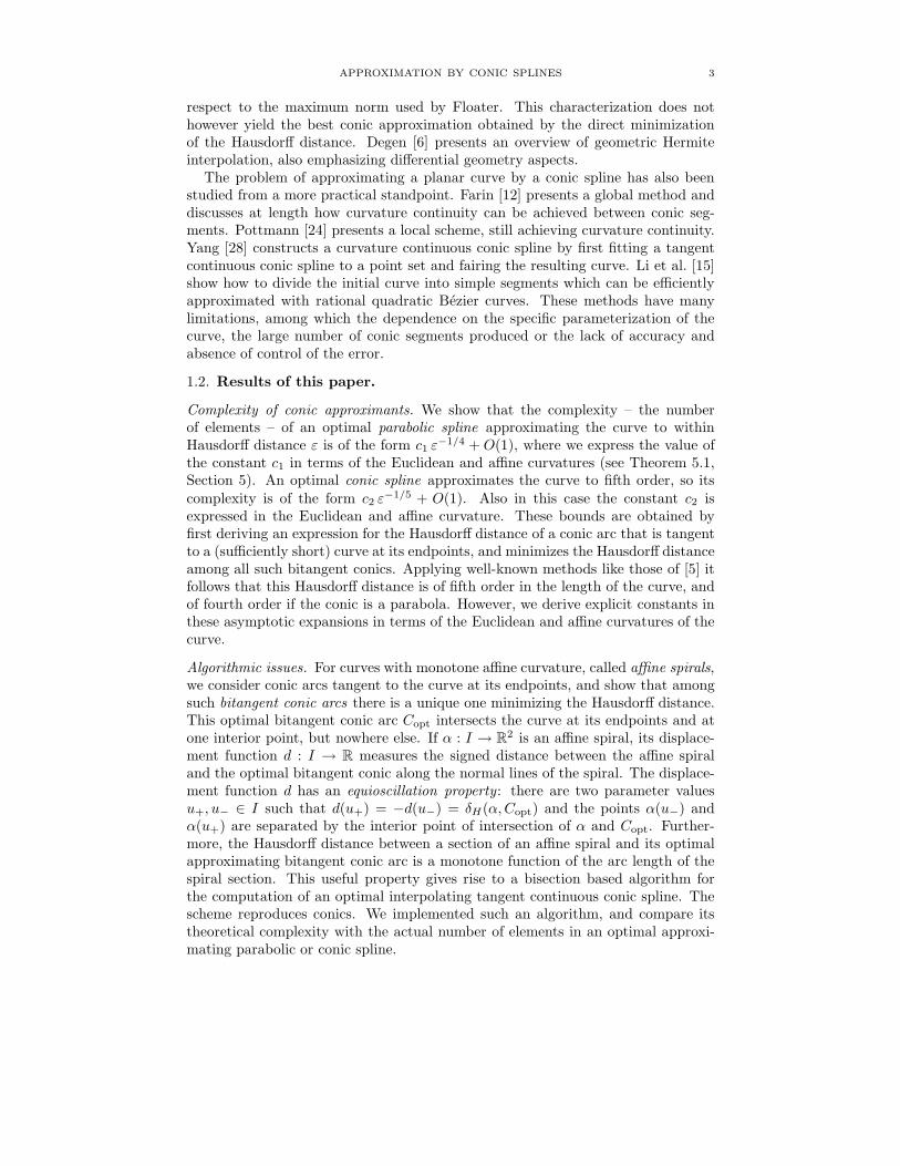
respect to the maximum norm used by Floater. This characterization does nothowever yield the best conic approximation obtained by the direct minimizationof the Hausdorff distance. Degen [6] presents an overview of geometric Hermiteinterpolation, also emphasizing differential geometry aspects.

The problem of approximating a planar curve by a conic spline has also beenstudied from a more practical standpoint. Farin [12] presents a global method anddiscusses at length how curvature continuity can be achieved between conic seg-ments. Pottmann [24] presents a local scheme, still achieving curvature continuity.Yang [28] constructs a curvature continuous conic spline by first fitting a tangentcontinuous conic spline to a point set and fairing the resulting curve. Li et al. [15]show how to divide the initial curve into simple segments which can be efficientlyapproximated with rational quadratic Bezier curves. These methods have manylimitations, among which the dependence on the specific parameterization of thecurve, the large number of conic segments produced or the lack of accuracy andabsence of control of the error.

1.2. Results of this paper.

Complexity of conic approximants. We show that the complexity – the numberof elements – of an optimal parabolic spline approximating the curve to withinHausdorff distance ε is of the form c1 ε

−1/4 + O(1), where we express the value ofthe constant c1 in terms of the Euclidean and affine curvatures (see Theorem 5.1,Section 5). An optimal conic spline approximates the curve to fifth order, so itscomplexity is of the form c2 ε

−1/5 + O(1). Also in this case the constant c2 isexpressed in the Euclidean and affine curvature. These bounds are obtained byfirst deriving an expression for the Hausdorff distance of a conic arc that is tangentto a (sufficiently short) curve at its endpoints, and minimizes the Hausdorff distanceamong all such bitangent conics. Applying well-known methods like those of [5] itfollows that this Hausdorff distance is of fifth order in the length of the curve, andof fourth order if the conic is a parabola. However, we derive explicit constants inthese asymptotic expansions in terms of the Euclidean and affine curvatures of thecurve.

Algorithmic issues. For curves with monotone affine curvature, called affine spirals,we consider conic arcs tangent to the curve at its endpoints, and show that amongsuch bitangent conic arcs there is a unique one minimizing the Hausdorff distance.This optimal bitangent conic arc Copt intersects the curve at its endpoints and atone interior point, but nowhere else. If α : I → R

2 is an affine spiral, its displace-ment function d : I → R measures the signed distance between the affine spiraland the optimal bitangent conic along the normal lines of the spiral. The displace-ment function d has an equioscillation property: there are two parameter valuesu+, u− ∈ I such that d(u+) = −d(u−) = δH(α,Copt) and the points α(u−) andα(u+) are separated by the interior point of intersection of α and Copt. Further-more, the Hausdorff distance between a section of an affine spiral and its optimalapproximating bitangent conic arc is a monotone function of the arc length of thespiral section. This useful property gives rise to a bisection based algorithm forthe computation of an optimal interpolating tangent continuous conic spline. Thescheme reproduces conics. We implemented such an algorithm, and compare itstheoretical complexity with the actual number of elements in an optimal approxi-mating parabolic or conic spline.


1.3. Paper overview. Section 2 reviews some notions from affine differential ge-ometry. In particular, we introduce affine arc length and affine curvature, whichare invariant under equi-affine transformations. Conic arcs are the only curves inthe plane having constant affine curvature, which explains the relevance of thesenotions from affine differential geometry for our work. Section 3 introduces affinespirals, a class of curves which have a unique optimal bitangent conic. We showthat the displacement function, which measures the distance of the curve to its off-set curve along its normals, has an equioscillation property in the sense that it hasextremes at exactly two points on the curve. Furthermore, the Hausdorff distancebetween an arc of an affine spiral and its optimal bitangent conic arc is increasingin the length of this arc. This useful property gives rise to a bisection algorithm forthe computation of a conic spline approximating a smooth curve with a minimalnumber of elements. Section 6 presents the output of the algorithm for a collectionof examples. The main result of Section 4 is a relation between the affine curvaturesof a curve and a bitangent offset curve. We use this result in Section 5 to derive anexpression for the complexity of optimal parabolic and conic splines approximatinga regular curve. We do so by deriving a bound on the Hausdorff distance betweenan affine spiral arc and its optimal bitangent conic. We conclude with topics forfuture work in Section 7.Acknowledgements. We thank the referees for their helpful comments.

2. Preliminaries from differential geometry

Circular arcs and straight line segments are the only regular smooth curves inthe plane with constant Euclidean curvature. Conic arcs are the only smooth curvesin the plane with constant affine curvature. The latter property is crucial for ourapproach, so we briefly review some concepts and properties from affine differentialgeometry of planar curves. See also Blaschke [3].

2.1. Affine curvature. Recall that a regular curve α : J → R2 defined on a closed

real interval J , i.e., a curve with non-vanishing tangent vector T (u) := α′(u), isparameterized according to Euclidean arc length if its tangent vector T has unitlength. In this case, the derivative of the tangent vector is in the direction of theunit normal vector N(u), and the Euclidean curvature κ(u) measures the rate ofchange of T , i.e., T ′(u) = κ(u)N(u). Euclidean curvature is a differential invariantof regular curves under the group of rigid motions of the plane, i.e., a regular curveis uniquely determined by its Euclidean curvature, up to a rigid motion.

The larger group of equi-affine transformations of the plane, i.e., affine transfor-mations with determinant one (in other words, area preserving linear transforma-tions), also gives rise to a differential invariant, called the affine curvature of thecurve. To introduce this invariant, let I ⊂ R be an interval, and let γ : I → R

2 bea smooth, regular plane curve. We shall denote differentiation with respect to the

parameter u by a dot: α = dαdu , α = d2α

du2 , and so on. Then regularity means thatα(u) 6= 0, for u ∈ I. Let the reparameterization u(r) be such that γ(r) = α(u(r))satisfies

(2.1) [γ′(r), γ′′(r)] = 1.

Here [v, w] denotes the determinant of the pair of vectors {v, w}, and derivativeswith respect to r are denoted by dashes. The parameter r is called the affine


arc length parameter. If [α, α] 6= 0, in other words, if the curve α has non-zerocurvature, then α can be parameterized by affine arc length, and (2.1) implies that

(2.2) [α(u(r)), α(u(r))] u′(r)3 = 1.

Putting

(2.3) ϕ(u) = [α(u), α(u)]1/3,

we rephrase (2.2) as

(2.4) u′(r) =1

ϕ(u(r)).

From (2.1) it also follows that [γ′(r), γ′′′(r)] = 0, so there is a smooth function k

such that

(2.5) γ′′′(r) + k(r) γ′(r) = 0.

The quantity k(r) is called the affine curvature of the curve γ at γ(r). It is onlydefined at points of non-zero Euclidean curvature. A regular curve is uniquelydetermined by its affine curvature, up to an equi-affine transformation of the plane.

From (2.1) and (2.5) we conclude k = [γ′′, γ′′′]. The affine curvature of α atu ∈ I is equal to the affine curvature of γ at r, where u = u(r).

2.2. Affine Frenet-Serret frame. The well known Frenet-Serret identity for theEuclidean frame, namely

(2.6) α = T, T = κN, N = −κT,

where the dot indicates differentiation with respect to Euclidean arc length, havea counterpart in the affine context. More precisely, let α be a strictly convex curveparameterized by affine arc length. The affine Frenet-Serret frame {t(r), n(r)} ofα is a moving frame at α(r), defined by t(r) = α′(r), and n(r) = t′(r), respectively.Here the dash indicates differentiation with respect to affine arc length. The vectort is called the affine tangent, and the vector n is called the affine normal of thecurve. The affine frame satisfies

(2.7) α′ = t, t′ = n, n′ = −k t.

Furthermore, we have the following identity relating the affine moving frame {t, n}and the Frenet-Serret moving frame {T,N}.

Lemma 2.1. 1. The affine arc length parameter r is a function of the Euclideanarc length parameter s satisfying

(2.8)dr

ds= κ(s)1/3.

2. The affine frame {t, n} and the Frenet-Serret frame {T,N} are related by

(2.9) t = κ−1/3 T, n = − 13 κ

−5/3 κ T + κ1/3N.

Here κ is the derivative of the Euclidean curvature with respect to Euclidean arclength.


Proof. 1. Let γ(r) be the parametrization by affine arc length, and let α(s) =γ(r(s)) be the parametrization by Euclidean arc length. Then α = T and α = κN .Again we denote derivatives with respect to Euclidean arc length by a dot. Sinceγ′ = t and t′ = γ′′ = n, we have

(2.10) T = α = rt, and N = κ−1 α = κ−1(rt+ (r)2n)

Since [T,N ] = 1, and [t, n] = 1, we obtain 1 = κ−1r3. This proves the first claim.

2. The first part of the lemma implies r = 13 κ

−2/3 κ. Plugging this into the iden-tity (2.10) yields the expression for the affine Frenet-Serret frame in terms of theEuclidean Frenet-Serret frame. �

The affine Frenet-Serret identities (2.7) yield the following values for thederivatives—with respect to affine arc length—of α up to order five, which willbe useful in the sequel:

(2.11)α′ = t, α′′ = n, α′′′ = −k t,

α(4) = −k′ t− k n, α(5) = (k2 − k′′) t− 2k′ n.

Combining these identities with the Taylor expansion of α at a given point yieldsthe following affine local canonical form of the curve.

Lemma 2.2. Let α : I → R2 be a regular curve with non-vanishing curvature, and

with affine Frenet-Serret frame {t, n}. Then

α(r0 + r) = α(r0) +(r − 1

3! k0 r3 − 1

4! k′0 r

4 +O(r6))t0

+(

12 r

2 − 14! k0 r

4 − 25! k

′0 r

5 +O(r6))n0,

where t0, n0, k0, and k′0 are the values of t, n, k and k′ at r0.Furthermore, in its affine Frenet-Serret frame the curve α can be written locally

as x t0 + y(x)n0, with

y(x) = 12 x

2 + 18 k0 x

4 + 140 k

′0x

5 +O(x6).

The first identity follows directly from (2.11). As for the second, it follows fromthe first by a series expansion. Indeed, write

x = r − 13! k0 r

3 − 14! k

′0 r

4 +O(r6).

Computing the expansion of the inverse function gives

r = x+ 13! k0 x

3 + 14! k

′0 x

4 +O(x6).

Plugging in y = 12 r

2 − 14! k0 r

4 − 25! k

′0 r

5 +O(r6) gives the result.

2.3. Affine curvature of curves with arbitrary parameterization. The fol-lowing proposition gives an expression for the affine curvature of a regular curve interms of an arbitrary parameterization. See also [3, Chapter 1.6].

Proposition 2.3. Let α : I → R2 be a regular C4-curve with non-zero Euclidean

curvature. Then the affine curvature k of α is given by

(2.12) k =1

ϕ5[α,

...α ] +

ϕ ϕ− 3ϕ2

ϕ4,

where ϕ = [α, α]1/3.

For a proof of this result we refer to Appendix A.


Remark. Proposition 2.3 gives the following expression for the affine curvature k interms of the Euclidean curvature κ:

k =9 κ4 − 5 (κ)2 + 3 κ κ

9 κ8/3,

where κ and κ are the derivatives of the Euclidean curvature with respect to arclength. This identity is obtained by observing that, for a curve parameterizedby Euclidean arc length, the function ϕ is given by ϕ = κ1/3. This follows fromthe Frenet-Serret identities (2.6) and the definition (2.3) of ϕ. Substituting thisexpression into (2.12) yields the identity for k in terms of κ.

2.4. Conics have constant affine curvature. Solving the differential equa-tion (2.5) shows that a curve of constant affine curvature is a conic arc. Moreprecisely, a curve with constant affine curvature is a hyperbolic, parabolic, or ellip-tic arc iff its affine curvature is negative, zero, or positive, respectively.

We now give expressions for the (constant) affine curvature of conics defined byan implicit quadratic equation.

Proposition 2.4 ([22], Theorem 6.4). The affine curvature of the conic defined bythe quadratic equation

ax2 + 2bxy + cy2 + 2dx+ 2ey + f = 0

is given by k = S T−2/3, where

S =

∣∣∣∣

a b

b c

∣∣∣∣, T =

∣∣∣∣∣∣

a b d

b c e

d e f

∣∣∣∣∣∣

.

The next result relates the affine curvatures of a regular curve in the plane andits image under linear transformations.

Lemma 2.5. Let α be the image of a regular planar curve β under a linear trans-formation x 7→ Ax. The affine curvatures kα and kβ of the curves α and β are

related by kα = (detA)−2/3 kβ.

Proof. Assume that β is parameterized by affine arc length. Since α(u) = Aβ(u),

it follows that the function ϕ, defined by (2.3), satisfies ϕ = [Aβ,Aβ]1/3

=

(detA)1/3[β, β]1/3

= (detA)1/3. According to Proposition 2.3 the affine curvature

of α is given by kα = (detA)−5/3 [Aβ,A...β ] = (detA)−2/3 kβ . �

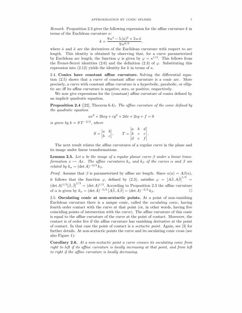
2.5. Osculating conic at non-sextactic points. At a point of non-vanishingEuclidean curvature there is a unique conic, called the osculating conic, havingfourth order contact with the curve at that point (or, in other words, having fivecoinciding points of intersection with the curve). The affine curvature of this conicis equal to the affine curvature of the curve at the point of contact. Moreover, thecontact is of order five if the affine curvature has vanishing derivative at the pointof contact. In that case the point of contact is a sextactic point. Again, see [3] forfurther details. At non-sextactic points the curve and its osculating conic cross (seealso Figure 1):

Corollary 2.6. At a non-sextactic point a curve crosses its osculating conic fromright to left if its affine curvature is locally increasing at that point, and from leftto right if the affine curvature is locally decreasing.


Figure 1. The curve and its osculating conic (dashed). The affinecurvature is increasing in the left picture, and decreasing in theright picture.

2.6. The five-point conic. To derive error bounds for an optimal approximatingconic we use the property that the approximating conic depends smoothly on thepoints of intersection with the curve. More precisely, let α : I → R

2 be a regularcurve without sextactic points, and let si, 1 6 i 6 5, be points on I, not necessarilydistinct. The unique conic passing through the points α(si) is denoted by Cs, withs = (s1, s2, s3, s4, s5). If one or more of the points coincide, the conic has contactwith the curve of order corresponding to the multiplicity of the point. For instance,if s1 = s2 6= si, i > 3, then Cs has first order contact with (is tangent to) the curveat α(s1).

If si 6= sj, for i 6= j, then the implicit quadratic equation of this conic canbe obtained as follows. Let the Veronese mapping Ψ : R

2 → R6 be defined by

Ψ(x) = (x21, x1x2, x

22, x1, x2, 1), x = (x1, x2), then the equation of the conic Cs is

f(x, s) = 0, with

(2.13) f(x, s) = det(Ψ(x),Ψ(α(s1)),Ψ(α(s2)),Ψ(α(s3)),Ψ(α(s4)),Ψ(α(s5))

).

However, if si = sj for i 6= j, then f(x, s) = 0. We obtain a quadratic equation ofthe conic Cs by (formally) dividing f(x, s) by si − sj . More precisely:

Lemma 2.7. If α is a Cm-curve, m > 4, then the conic Cs has a quadratic equationwith coefficients that are Cm−4-functions of s = (s1, s2, s3, s4, s5) ∈ R

5.

Proof. Put ψ(s) = Ψ(α(s)). The Newton development of ψ in terms of the divideddifferences of ψ up to order four associated with the points s1, . . . , s5 is given by

ψ(sk) = ψ(s1) +∑k

i=2

∏i−1j=1(sk − sj) [s1, . . . , sk]ψ, for 2 6 k 6 5. See Appendix B.

Plugging these identities into (2.13), we see that f(x, s) =∏

16j<k65

(sk−sj)F (x, s),

withF (x, s) = det(Ψ(x), ψ(s1), [s1, s2]ψ, . . . , [s1, . . . , s5]ψ).

Since ψ is Cm, with m > 4, it follows from Appendix B that F is a Cm−4-function,with x 7→ F (x, s) being a non-vanishing quadratic function. �

In particular, if σ = (σ, . . . , σ) ∈ R5, then it follows from Appendix B,

Lemma B.1, that

F (x, σ) =1

2!3!4!det(Ψ(x), ψ(σ), ψ′(σ), ψ′′(σ), ψ′′′(σ), ψ(4)(σ)

).

Since α contains no sextactic points, the equation F (x, σ) = 0 defines a non-degenerate conic, the osculating conic at α(σ).

If σ, and u are three distinct points of I, then there is a unique conic Cσ,,u

which is tangent to α at α(σ) and α(), and passes through the point α(u). Theequation of this conic is

det(Ψ(x), ψ(σ), ψ′(σ), ψ(), ψ′(), ψ(u)

)= 0.


As in the proof of Lemma 2.7 one proves that Cσ,,u is a Cm−4-function of (σ, , u),and that it tends to the osculating conic at α(σ) as u→ σ and → σ.

3. Optimal conic approximation of affine spiral arcs

In this section we prove both the equioscillation property and the monotonicityproperty of the Hausdorff distance. Both properties are global, since the affine spiralis not necessarily short.

3.1. Intersections of conics and affine spirals. We start with a useful globalproperty of affine spirals.

Proposition 3.1. (1) A conic intersects an affine spiral in at most five points,counted with multiplicity.

(2) The osculating conics of an affine spiral are disjoint, and do not intersectthe spiral arc except at their point of contact.

A proof of this theorem is given in [23, chapter 4]. The second part is an exercisein [3, chapter 1]. A modern proof is given in [27].

Now consider an affine spiral arc α : [u0, u1] → R2. Let Cu, u0 6 u 6 u1, be

the unique conic that is tangent to α at its endpoints, and intersects it at the pointα(u). For u = u0 and u = u1 the conic has a triple intersection with the curve, or,in other words, it has contact of second order with α there.

Proposition 3.2. (1) Two conics Cu and Cu′ , u 6= u′, are tangent at α(u0)and α(u1), and have no other intersections.

(2) Conic Cu intersects arc α at α(u0), α(u), and α(u1), but at no other point.

Proof. 1. By Bezout’s theorem, two conics intersect in at most four points, countedwith multiplicity. Since conics Cu and Cu′ intersect with multiplicity two at eachof the points α(u0) and α(u1), there are no other intersections.

2. This is a straightforward consequence of Proposition 3.1, part 1.�

3.2. Displacement function. A bitangent conic of a regular curve α : I → R2

is a conic arc which is tangent to α at its endpoints, such that each normal lineof α intersects the conic arc in a unique point. Therefore, a bitangent conic has aparameterization β : I → R

2 of the form β(u) = α(u)+d(u)N(u), where d : I → R

is the displacement function of the conic arc. The Hausdorff distance between α

and a bitangent conic C is equal to

δH(α,C) = maxu∈I |d(u)|.

There is a one-parameter family of bitangent conics, so the goal is to determine anoptimal bitangent conic, i.e., a conic in this family that minimizes the Hausdorffdistance.

3.3. Equioscillation property. Denote the arc of the curve between α(u0) andα(u) by α−

u , and the arc between α(u) and α(u1) by α+u . Similarly, C−

u and C+u

denote the arcs of Cu between α(u) and α(u0) and between α(u) and α(u1), re-spectively.


α(u0)

α(u1)

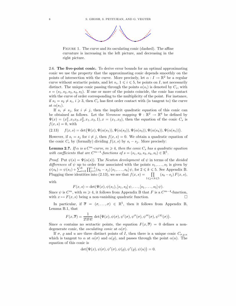
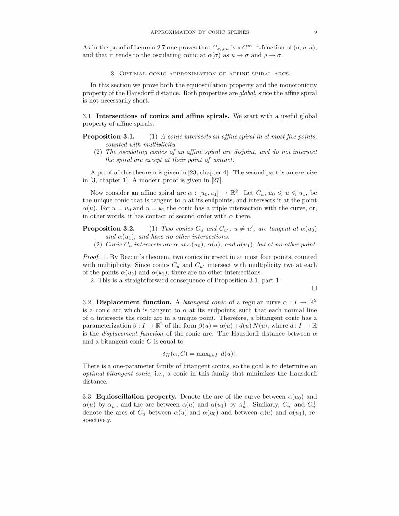
Figure 2. The curve and the family of conics Cu, u0 6 u 6 u1,tangent at the endpoints α(u0) and α(u1) and passing throughα(u).

Figure 3. The graphs of the family of displacement functions.The bold graph corresponds to the displacement function of theoptimal conic.

Corollary 3.3 (Equioscillation property). There is a unique conic Cu∗in the

family Cu, u0 6 u 6 u1, such that the Hausdorff distance du∗of α and Cu∗

isminimal:

du∗= minu06u6u1

δH(α,Cu).

Furthermore,

du∗= δH(α−

u∗, C−

u∗) = δH(α+

u∗, C+

u∗).

Proof. Let δ±(u) = δH(α±u , C

±u ). Then there are two cases: (i) δ−(u) is increasing

and δ+(u) is decreasing as a function of u, and (ii) δ−(u) is decreasing and δ+(u)is increasing as a function of u. The situation depicted in Figure 2 correspondsto Case (i). This observation, which is a direct consequence of Proposition 3.2,part 2, implies that there is a unique u∗ such that δ−(u∗) = δ+(u∗). Obviously,du∗

satisfies the two claimed identities. �

Let d(s;u), u0 6 s, u 6 u1, be the displacement function defined by the conditionthat the point α(s) + d(s;u)N(s), lies on the conic arc Cu. Here N(s) is the unitnormal of the curve at α(s). The graphs of the functions s 7→ d(s;u), u0 6 s 6 u1,are disjoint, except at their endpoints. See Figure 3. We conjecture that thedisplacement function of an affine spiral is bimodal, i.e., its displacement functionhas the profile of any of the graphs depicted in Figure 3. More precisely, thefunction has one maximum, one minimum, and one interior zero, and there are noother interior extremal points.


3.4. Monotonicity of optimal Hausdorff distance. If one endpoint of the affinespiral moves along the curve α, the Hausdorff distance between the affine spiral andits optimal bitangent conic arc is monotone in the arc length of the affine spiral.This result shows that bisection methods can be used for the computation of anoptimal approximating conic arc. We use this property for the implementation ofthe algorithm presented in Section 6.

Proposition 3.4 (Monotonicity of Hausdorff distance along spiral arcs). Let α :I → R

2 be an affine spiral arc, where I is an open interval containing 0. For > 0let α be the sub-arc between α(0) and α(), and let β be the (unique) conic arctangent to α at its endpoints, and minimizing the Hausdorff distance between α

and the conic arcs tangent to α at its endpoints. Then the Hausdorff distancebetween α and β is a monotonically increasing function of , for > 0.

Proof. First we introduce some notation. The unique interior point of intersectionof α and β occurs at u = u() ∈ I. The sub-arcs of α and β between α(0) andα(u()) are denoted by α−

and β− , respectively. The complementary sub-arcs of

α and β are denoted by α+ and β+

, respectively. According to the EquioscillationProperty (Corollary 3.3) the Hausdorff distance between α and β is equal to theHausdorff distances between α±

and β± , and is attained as the distance between

points a±() on α± and b±() on β±

, i.e.,

δH(α, β) = dist(a−(), b−()) = dist(a+(), b+()).

The complete conic containing β will be denoted by K. We will repeatedly usethe following consequence of Bezout’s theorem:

Intersection Property: For 0 < 1 < 2, the conics K1and K2

have at mosttwo points of intersection (possibly counted with multiplicity) different from α(0).

Let 1, 2 ∈ I, with 0 < 1 < 2. The regions bounded by α±2

and β±2

are denoted

by R±. Since K1is either compact or unbounded, and not disjoint from the

boundary of R+, it intersects this boundary in an even number of points (countedwith multiplicity). Our strategy is to prove that β−

1lies inside R−, or that β+

1lies

inside R+. In the former case, we see that

δH(α1, β1

) = dist(a−(1), b−(1)) < dist(a−(2), b−(2)) = δH(α2, β2

),

whereas in the latter case

δH(α1, β1

) = dist(a+(1), b+(1)) < dist(a+(2), b+(2)) = δH(α2, β2

).

We distinguish two cases, depending on the order of u(1) and u(2).

Case 1: u(1) > u(2). Note that the conic K1is tangent to α at α(1), a point

contained in α2. Therefore, in this case K1

intersects α+2

in an odd number ofpoints, namely, once at the point α(u(1)) and twice at the point of tangency α(1).β+

2, the other part of boundary of R+, in an odd number of points. By the

Intersection Property, this odd number is equal to one. Since both endpoints of β1

lie on the same side of β2, this point of intersection does not lie on β1

. In otherwords, the interior of β+

1lies inside the region R+.

Case 2: u(1) < u(2). In this case K1does not cross α+

2, since it intersects α+

2

in two coinciding points at the tangency α(1), but at no other point. Therefore,K1

intersects β+2

, the other part of the boundary of R+, in at least two points (atleast one entrance and at least one exit point). By the Intersection Property, apart


from α(0), these are the only points in which K1and K2

intersect. Therefore,β−

1intersects neither β−

2nor α−

2in an interior point. In other words, the interior

of β−1

lies inside the region R−. �

Remark. A similar monotonicity property holds for the Hausdorff distance betweenan affine spiral and a bitangent parabolic arc. The proof is omitted, since it isstraightforward, and along the same lines as the proof of Proposition 3.4.

4. Affine curvature of offset curves

The main result of this section is a relation between the affine curvatures of acurve and a bitangent offset curve.

Let α : I → R2 be a regular curve parameterized by affine arc length, with affine

arc length parameter u ∈ I. Here I is an open interval, containing 0. We consideroffset curves tangent to α at α(0) and α(). The affine curvature of such a curve isrelated to the affine curvature k of α, as indicated in the first part of the followingLemma. In the second part, an analogous result relates these curvatures when thereis an additional point of intersection at α(σ).

Lemma 4.1 (Affine curvature of offset curves). Let α be a Cm-regular curve.1. Let β : I × I → R

2 be a Cn-function, such that, β(·, ) is a curve tangent to αat α(0) and α(), for ∈ I. If m,n > 5, there are Cl-functions P,Q : I × I → R,with l = min(m− 5, n− 4), such that

(4.1) β(u, ) = α(u) + d(u, )(P (u, )t(u) +Q(u, )n(u)

),

where d(u, ) = u2 (u−)2. Here t(u) and n(u) are the affine tangent and the affinenormal of α, respectively. Furthermore, the affine curvature kβ(u, ) of β(·, ) at0 6 u 6 is given by

(4.2) kβ(u, ) = k(0) + 8Q(0, 0) +O().

2. Let β : I × I × I → R2 be a Cn-function, such that, β(·, σ, ) is a curve tangent

to α at α(0) and α() and intersecting α at α(σ), for σ, ∈ I and 0 6 σ 6 . Ifm,n > 6, and, moreover, β also intersects α at α(σ), with 0 6 σ 6 , then thereare Cl-functions P,Q : I × I → R, with l = min(m− 6, n− 5), such that

(4.3) β(u, σ, ) = α(u) + d(u, σ, )(P (u, σ, )t(u) +Q(u, σ, )n(u)

),

where d(u, σ, ) = u2 (u− )2 (u− σ). Furthermore, the affine curvature kβ(u, σ, )of β(·, σ, ) at 0 6 u 6 is given by

kβ(u, σ, ) = k(0) + k′(0)u+ 8 (5u− σ − 2)Q(0, 0, 0) +O(2).

Proof. 1. If α is Cm, then the functions (u, ) 7→ [β(u, ) − α(u), n(u)] and(u, ) 7→ [β(u, ) − α(u), t(u)] are of class Cmin(m−1,n). For fixed , these functionshave double zeros at u = 0 and u = . The Division Property, cf. Appendix B,Lemma B.2, guarantees the existence of Cmin(m−5,n−4)-functions P andQ satisfying[β(u, ) − α(u), n(u)] = d(u, )P (u, ) and [β(u, ) − α(u), t(u)] = d(u, )Q(u, ).In other words, P and Q satisfy identity (4.1).

According to Proposition 2.3 the affine curvature of the curve β(·, ) is a Cn−4-function given by

(4.4) kβ =1

ϕ5[βuu, βuuu] +

1

ϕ4(ϕuu ϕ− 3ϕ2

u),


ϕ = [βu, βuu]1/3. In (4.4), the functions kβ , ϕ, β, and their partial derivativesare evaluated at (u, ). Since n > 5, and 0 6 u 6 , it follows that kβ(u, ) =kβ(u, 0) + O(). So, to prove (4.2), it is sufficient to determine β(u, 0) and itsderivatives up to order four. Writing β0(u) = β(u, 0), we see that

β0(u) = α(u) + f(u) (P0 t(u) +Q0 n(u)) +O(u5),

where f(u) = u4, P0 = P (0, 0) and Q0 = Q(0, 0). In view of the affine Frenet-Serretidentities (2.7) we get

β′0 = (1 + f ′ P0) t+ f ′Q0 n+O(u4),

β′′0 = f ′′ P0 t+ (1 + f ′′Q0)n+O(u3),(4.5)

β′′′0 = (−k + f ′′′ P0) t+ f ′′′Q0 n+O(u2).

Here the functions β0, f , t, n and k, as well as their derivatives, are evaluated at

u. Since ϕ(u, 0) = [β′0(u), β

′′0 (u)]

13 , we use the first two identities of (4.5) to derive

ϕ(u, 0) = 1 + 13 f

′′(u)Q0 +O(u3) = 1 + 4 u2Q0 +O(u3).

Similarly, using the second and third identity of (4.5) we get

[β′′0 (u), β′′′

0 (u)] = k(u) +O(u) = k(0) + 8Q0 +O(u).

Identity (4.2) is obtained by plugging these expressions into (4.4).

2. Now we turn to the case where the offset curve not only is tangent to α at itsendpoints, but also has an additional point of intersection at α(σ). The existenceof functions P and Q satisfying (4.3) is proven as in Part 1, using the DivisionProperty. Again the affine curvature of β is given by (4.4), where this time thefunctions kβ , ϕ, β, and their partial derivatives are evaluated at (u, σ, ).

In (4.3) we have d(u, σ, ) = u5 − (2+ σ)u4 +O(2 + σ2), P = P0 +O(u), andQ = Q0 +O(u). Focusing on the essential terms only, we rewrite (4.3) as:

(4.6) β = α+(u5− (2+σ)u4) (P0 t+Q0 n)+O(u6)+O((+σ)u5)+O(2 +σ2).

Here α, t and n are evaluated at u, and β at (u, σ, ). For a smoother presentation,we introduce the following terminology. The class Oi(u, σ, ), 0 6 i 6 4, consists ofall Cm−i-functions of the form O(u6−i) +O((+ σ)u5−i) +O(2 + σ2). Using thisnotation we rewrite (4.6) as

β = α+ f (P0 t+Q0 n) +O0(u, σ, ).

where f(u, σ, ) = u5 − (2+ σ)u4.If g ∈ Oi(u, σ, ), then gu ∈ Oi+1(u, σ, ), for 1 6 i 6 4. Therefore, we get, as

in (4.5):

βu = (1 + fu P0) t+ fuQ0 n+O1(u, σ, ),

βuu = fuu P0 t+ (1 + fuu Q0)n+O2(u, σ, ),(4.7)

βuuu = (−k + fuuu P0) t+ fuuuQ0 n+O3(u, σ, ).

Since ϕ = [βu, βuu]13 , we use the first two identities of (4.7) to derive

ϕ = 1 + 13 fuuQ0 +O2(u, σ, ),

so ϕ = 1 + O3(u, σ, ), ϕ2u = O4(u, σ, ), and ϕuu = 1

3 Q0 fuuuu + O4(u, σ, ).Similarly, using the second and third identity of (4.5) we get

[βuu, βuuu] = k(u) +O4(u, σ, ).


It follows that

kβ(u, σ, ) = k(u) + 13 fuuuu Q0 +O4(u, σ, )

= k(0) + k′(0)u+ 8 (5u− σ − 2)Q0 +O(2).

Note that in the last identity we used that O4(u, σ, ) = O(u2 + σ2 + 2) = O(2),since 0 6 u, σ 6 . This concludes the proof of the second part. �

If the offset curves are bitangent conics, the affine curvature of these conics canbe expressed in the Euclidean and affine curvature of the curve α at the points ofintersection. Furthermore, we can determine the displacement function up to termsof order five if the conic is a parabola, and up to terms of order six in the generalcase. These results will enable us to determine an asymptotic expression for theHausdorff distance between a small arc and its optimal bitangent conic.

Corollary 4.2 (Bitangent conics). Let α be a strictly convex regular Cm-curve.

1. If m > 8, a parabolic arc tangent to α at α(0) and α() has the form

(4.8) β(u, ) = α(u) + u2 (− u)2D(u, )N(u),

where D is a Cm−8-function with D(0, 0) = − 18 k(0)κ(0)1/3. Here N(u) is the

Euclidean normal of α, and κ is its Euclidean curvature.

2. If m > 9, a conic arc tangent to α at α(0) and α() and intersecting at α(σ),with 0 6 σ 6 , has the form

(4.9) β(u, σ, ) = α(u) + u2 (− u)2 (u− σ)D(u, σ, )N(u),

where D is a Cm−9-function with D(0, 0, 0) = − 140 k

′(0)κ(0)1/3. Moreover, itsaffine curvature is of the form

kβ(σ, ) = 15 (2k(0) + k(σ) + 2k()) +O(2).

Proof. 1. Obviously, the family of parabolic arcs can be written in the form β(u, ) =α(u) + d(u, )N(u), provided is sufficiently small. According to Lemma 2.7, βis a Cm−4-function, so d = [T, β − α] is a Cm−4-function with double zeros atu = 0 and u = . According to Lemma 4.1, the parabola has a parameterization ofthe form (4.1), where P and Q are Cm−8-functions. Therefore, d(u, ) = u2 (u −)2Q(u, ) [T (u), n(u)], so β is of the form (4.8) with D = Q [T, n]. In particular, Dis a Cm−8-function. Comparing this expression with identity (4.1) in Lemma 4.1,we see that D(u, ) = Q(u, ) [T (u), n(u)]. From (2.9) we conclude that D(0, 0) =κ(0)1/3Q(0, 0). Since the affine curvature of a parabolic arc is identically zero,Part 1 of Lemma 4.1 yields Q(0, 0) = − 1

8 k(0), yielding the value for D(0, 0) statedin Part 1.

2. As in Part 1 we prove that β has a parameterization of the form (4.9), where Dis a Cm−9-function. The affine curvature of a conic arc is constant, so Part 2of Lemma 4.1 yields Q(0, 0, 0) = − 1

40 k′(0). Since also in this case we have

D(0, 0, 0) = κ(0)1/3Q(0, 0, 0), we conclude that D(0, 0, 0) has the value stated inPart 2. Furthermore, (4.2) yields

kβ = k(0) + 15 (σ + 2) k′(0) +O(2) = 1

5 (2k(0) + k(σ) + 2k()) +O(2).

This concludes the proof of the second part. �


Remarks. 1. The second part of Corollary 4.2 can be generalized in the sense thatthe affine curvature of a conic intersecting a strictly convex arc at five points isequal to the average of the affine curvatures of the curve at these five points, upto quadratic terms in the affine length of the arc. The proof is similar to the onegiven above.

2. We conjecture that the ‘loss of differentiability’ is less than stated in Corollary 4.2.More precisely, we expect that D is of class Cm−4 for a bitangent parabolic arc,and of class Cm−5 for a bitangent conic arc.

5. Complexity of conic splines

In this section our goal is to determine the Hausdorff distance of a conic arc ofbest approximation to an arc of α of Euclidean length σ > 0, that is tangent toα at its endpoints. If the conic is a parabola, these conditions uniquely determinethe parabolic arc. If we approximate with a general conic, there is one degree offreedom left, which we use to minimize the Hausdorff distance between the the arcof α and the approximating conic arc β. As we have seen in Section 3, the optimalconic arc intersects the arc of α in an interior point.

The main result of this section gives an asymptotic bound on this Hausdorffdistance.

Theorem 5.1 (Error in parabolic and conic spline approximation). Let β be aconic arc tangent at its endpoints to an arc of a regular curve α of length σ, withnon-vanishing Euclidean curvature.

1. If α is a C8-curve, and β is a parabolic arc, then the Hausdorff distance betweenthese arcs has asymptotic expansion

(5.1) δH(α, β) = 1128 |k0|κ5/3

0 σ4 +O(σ5),

where κ0 and k0 are the Euclidean and affine curvatures of α at one of its endpoints,respectively.

2. If α is a C9-curve, and β is a conic arc, then the Hausdorff distance betweenthese arcs is minimized if the affine curvature of β is equal to the average of theaffine curvatures of α at its endpoints, up to quadratic terms in the length of α. Inthis case this Hausdorff distance has asymptotic expansion

(5.2) δH(α, β) = 12000

√5|k′0|κ2

0 σ5 +O(σ6),

where κ0 is the Euclidean curvature of α at one of its endpoints, and k′0 is thederivative of the affine curvature of α at one of its endpoints.

Proof. 1. According to Corollary 4.2, the parabolic arc has a parameterization of theform (4.8). It follows from Appendix C, Lemma C.1, applied to the displacementfunction d(u) = u2 (− u)2D(u, ), cf. (4.8), that

(5.3) δH(α, β) = 116 |D(0, 0)| 4 +O(5).

From Lemma 2.1, part 1, we derive

(5.4) = κ1/30 σ +O(σ2).

Since D(0, 0) = − 18 k(0)κ(0)1/3, we conclude from (5.3) and (5.4) that the Haus-

dorff distance satisfies (5.1).


2. Again, according to Corollary 4.2, cf. (4.9), a best approximating conic arc hasa parameterization of the form (4.9), with D(0, 0, 0) = − 1

40 k′(0)κ(0)1/3. Applying

Appendix C, Lemma C.1 to the displacement function d(u) = u2 (u − σ) ( −u)2D(u, σ, ), cf. (4.9), we see that

(5.5) δH(α, β) = 150

√5|D(0, 0, 0)| 5 +O(6),

where the optimal conic intersects the curve α for σ = σ() = 12 +O(2). Identities

(5.4) and (5.5) imply that the Hausdorff distance is given by (5.2). Finally, the affinecurvature of this conic is

15 (2k(0) + k(1

2 +O(2)) + 2k()) +O(2) = 12 (k(0) + k()) +O(2).

This concludes the proof of the main theorem of this section. �

Remark. It would be interesting to give a direct geometric proof of the fact thatthe best approximating conic has affine curvature equal to the average of the affinecurvatures of α at its endpoints.

The preceding result gives an asymptotic expression for the minimal number ofelements of an optimal parabolic or conic spline in terms of the maximal Hausdorffdistance.

Corollary 5.2 (Complexity of parabolic and conic splines). Let α : [0, L] → R2 be

a regular curve with non-vanishing Euclidean curvature of length L, parameterizedby Euclidean arc length, and let κ(s) and k(s) be its Euclidean and affine curvatureat α(s), respectively.

1. If α is a C8-curve, then the minimal number of arcs in a tangent continuousparabolic spline approximating α to within Hausdorff distance ε is

(5.6) N(ε) = c1

(∫ L

0

|k(s)|1/4 κ(s)5/12ds)

ε−1/4(1 +O(ε1/4)),

where c1 = 128−1/4 ≈ 0.297.

2. If α is a C9-curve, then the minimal number of arcs in a tangent continuousconic spline approximating α to within Hausdorff distance ε is

(5.7) N(ε) = c2

(∫ L

0

|k′(s)|1/5 κ(s)2/5ds)

ε−1/5(1 +O(ε1/5)),

where c2 = (2000√

5)−1/5 ≈ 0.186.

We only sketch the proof, and refer to the papers by McClure and Vitale [19]and Ludwig [17] for details about this proof technique in similar situations. Con-sider a small arc of α, centered at α(s). Let σ(s) be its Euclidean arc length.Then the Hausdorff distance between this curve and a bitangent parabolic arc is1

128 |k0|κ5/30 σ(s)4 +O(σ(s)5), cf. Theorem 5.1. Therefore,

σ(s) =4√

128 |k(s)|−1/4 κ(s)−5/12 ε1/4(1 +O(ε1/4)).

The first part follows from the observation that N(ε) =

∫ L

0

1

σ(s)ds. The proof of

the second part is similar.


6. Implementation

We implemented an algorithm in C++ using the symbolic computing libraryGiNaC

1, for the computation of an optimal parabolic or conic spline, based on themonotonicity property. For computing the optimal parabolic spline, the curve issubdivided into affine spirals. Then for a given maximal Hausdorff distance ε, thealgorithm iteratively computes optimal parabolic arcs starting at one endpoint. Ateach step of this iteration the next breakpoint is computed via a standard bisectionprocedure, starting from the most recently computed breakpoint. The bisectionprocedure yields a parabolic spline whose Hausdorff distance to the subtended arcis ε. An optimal conic spline is computed similarly. The bisection step is slightlymore complicated, since the algorithm has to select the optimal conic arc froma one-parameter family. Here the equioscillation property gives the criterion fordeciding whether the computed conic arc is optimal.

Below we present two examples of computations of optimal parabolic and conicsplines. We compare the computed number of elements of these splines with thetheoretical asymptotic complexity given in Corollary 5.2, thereby neglecting thehigher order terms in (5.6) and (5.7).

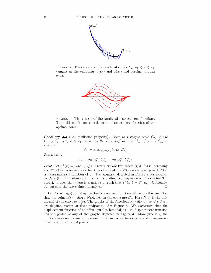
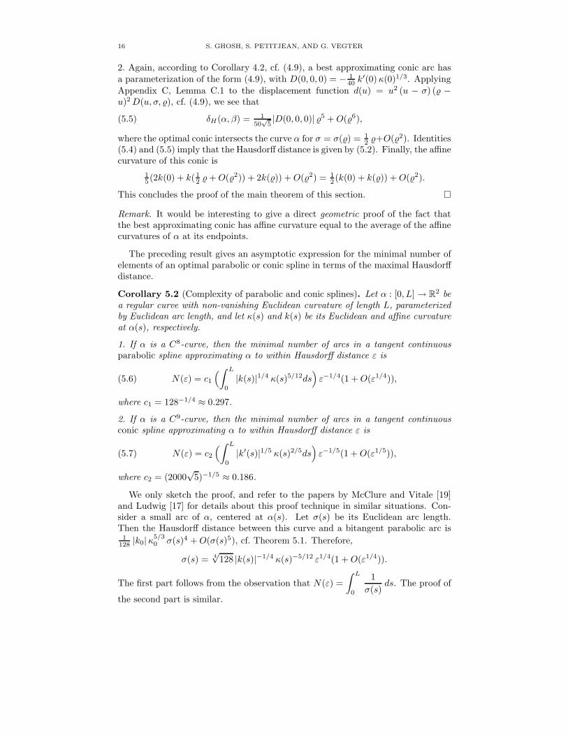
6.1. A spiral curve. We present the results of our algorithm applied to the spiralcurve, parameterized by α(t) = (t cos(t), t sin(t)), with 1

6π 6 t 6 2π.Figures 4(a) and 4(b) depict the result of the algorithm applied to the spiral

for different values of the error bound ε, for the approximation by conic arcs andparabolic arcs respectively. For ε > 10−2, there is no visual difference between thecurve and its approximating conic.

ε Parabolic ConicExp./ Th. Exp./ Th.

10−1 5 310−2 9 410−3 15 610−4 26 910−5 46 1310−6 82 2110−7 145 3210−8 257 51

Table 1. The complexity (number of arcs) of the parabolic splineand the conic spline approximating the Spiral Curve. The theoret-ical complexity matches exactly with the experimental complexity,for various values of the maximal Hausdorff distance ε.

Table 1 gives the number of arcs computed by the algorithm, and the theoreticalbounds on the number of arcs for varying values of ε, both for the parabolic andfor the conic spline.

6.2. Cayley’s sextic. We present the results of our algorithm applied to the Cay-ley’s sextic, the curve parameterized by α(t) = (4 cos( t

3 )3 cos(t), 4 cos( t3 )3 sin(t)),

1http://www.ginac.de


−1

31 4

−2

−2−3

0

−4

620 5

1

−3

−1 5420−2

1

−4

−3

3 6

−2

−1

1−1−3

0

−4

0

−1

32

−2

1

−3

−3 6−1 1 54

0

−2 20 1−1−2

1

6

−3

3−3 4

−1

−4

−2

5

0

−1

4

0

6

−2

−4

−3

1

−1−3 20−2 3 51 5

−4

4

0

−1

−1

1

−3

2−3

−2

1 60−2 3 6

−3

32

−2

−2 1−3

1

−1 5

−1

−4

0

40 0−2

1

6−1 2

−1

4 5

−4

−3

0

−2

3

−3

1

(a) Conic spline approximation

2

0

−2

−4

2 5

1

−1

−3

−5

640 1−2 3−1−3 2−1−3 −2 6

−2

1

1

−1

3

0

−3

−4

40 5

1

40 51 6−2 −1−3

−2

−1

0

2

−3

−4

3 4

−3

−4

−2

1

−3 −2 6−1 2

0

−1

5310

−3

−4

−1

1

2

−3

4

0

61 3−1 0

−2

5−2

−1

−2 4

−3

−2

−3 −1 0 6

0

1 5

−4

1

32

1

−1

62−3

−3

1 430

−4

−1

−2

0

5−2

(b) Parabolic spline approximation

Figure 4. Approximation of the spiral for ε ranging between 10−1

to 10−8.

with − 34 π 6 t 6 3

4 π. This curve has a sextactic point at t = 0. For all values of ε

we divide the parameter interval into two parts [− 34 π, 0] and [0, 3

4 π] each contain-ing the sextactic point as an endpoint, and then approximate with conic arcs usingthe Incremental Algorithm.

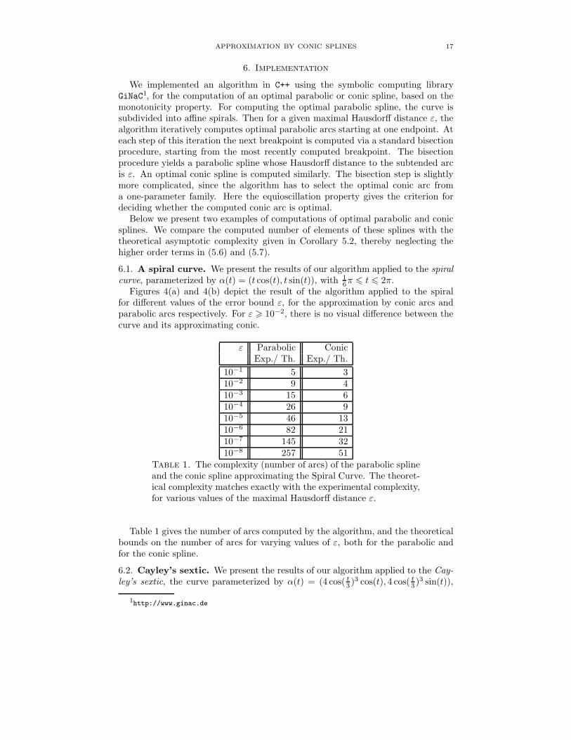
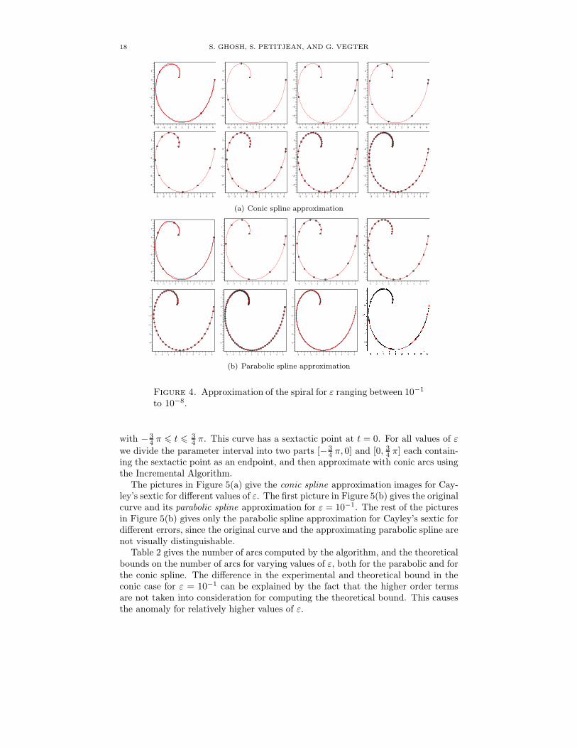
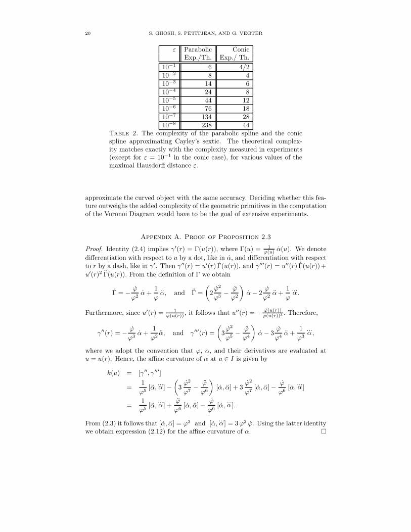
The pictures in Figure 5(a) give the conic spline approximation images for Cay-ley’s sextic for different values of ε. The first picture in Figure 5(b) gives the originalcurve and its parabolic spline approximation for ε = 10−1. The rest of the picturesin Figure 5(b) gives only the parabolic spline approximation for Cayley’s sextic fordifferent errors, since the original curve and the approximating parabolic spline arenot visually distinguishable.

Table 2 gives the number of arcs computed by the algorithm, and the theoreticalbounds on the number of arcs for varying values of ε, both for the parabolic and forthe conic spline. The difference in the experimental and theoretical bound in theconic case for ε = 10−1 can be explained by the fact that the higher order termsare not taken into consideration for computing the theoretical bound. This causesthe anomaly for relatively higher values of ε.


−1

2

−1

1

−3

0

0 41 2 3

3

−2

−1

1

−2

1

2

0

3

−1

3 420

−3

40 1

0

2

3

3

−3

−1

−1

−2

1

2

4

3

31−1

0

1

0

−3

2

−1

2

−2

−1

3 40

0

−2

1−1

2

1

3

−3

2 1

2

−2

4

−1

1

−1

−3

0

0 3

3

2 1

0

2

−3

3

1

0

−1

−2

432−1

2

3

4

−3

1

0

3−1

−2

2

1

−1

0

(a) Conic spline approximation

0

3

1

3−1

0

2

−1

−2

−3

4

2

1 4

−2

3

1

−3

0

0 2

2

−1

3−1

1

3

3

−1

42

−3

1

1

0

2

−2

−1 0 320

3

−1

−1

−2

2

1

0

4

−3

1

−1

1

−3

3

32 4

−2

1

0

0

2

−1

−1

3

−2

1

−1

2

0

1

3 42

0

−3 −3

−1

3

31

1

2

−2

2

0 4

0

−1

−2

−3

43−1

0

3

2

1

0 1

−1

2

(b) Parabolic spline approximation

Figure 5. Plot of the approximations of a part of Cayley’s sexticfor ε ranging from 10−1 to 10−8.

7. Future work

It would be interesting to determine the constants in the approximation order ofsome of the existing methods for geometric Hermite interpolation (Floater [14], Sch-aback [26]), using the methods of this paper. Another open problem is to determinemore terms in the asymptotic expansions of the complexity of optimal parabolicand conic splines derived in Section 5, like Ludwig [17] extends the complexitybound of the linear spline approximation of Fejes Toth [13].

To enable certified computation of conic arcs with guaranteed bounds on theHausdorff distance we would have to derive sharp upper bounds on the Hausdorffdistance between a curve and a bitangent conic, extending the asymptotic expressionfor these error bounds for short curves, as given in Theorem 5.1. Such a certifiedmethod could lead to robust computation of geometric structures for curved ob-jects, like its Voronoi Diagram. In this approach the curved object would first beapproximated by conic splines, after which the Voronoi Diagram of the conic arcsof these splines would be computed. The number of elements of such a conic splinewould be orders of magnitude smaller than the number of line segments needed to


ε Parabolic ConicExp./Th. Exp./ Th.

10−1 6 4/210−2 8 410−3 14 610−4 24 810−5 44 1210−6 76 1810−7 134 2810−8 238 44

Table 2. The complexity of the parabolic spline and the conicspline approximating Cayley’s sextic. The theoretical complex-ity matches exactly with the complexity measured in experiments(except for ε = 10−1 in the conic case), for various values of themaximal Hausdorff distance ε.

approximate the curved object with the same accuracy. Deciding whether this fea-ture outweighs the added complexity of the geometric primitives in the computationof the Voronoi Diagram would have to be the goal of extensive experiments.

Appendix A. Proof of Proposition 2.3

Proof. Identity (2.4) implies γ′(r) = Γ(u(r)), where Γ(u) = 1ϕ(u) α(u). We denote

differentiation with respect to u by a dot, like in α, and differentiation with respectto r by a dash, like in γ′. Then γ′′(r) = u′(r) Γ(u(r)), and γ′′′(r) = u′′(r) Γ(u(r))+

u′(r)2 Γ(u(r)). From the definition of Γ we obtain

Γ = − ϕ

ϕ2α+

1

ϕα, and Γ =

(

2ϕ2

ϕ3− ϕ

ϕ2

)

α− 2ϕ

ϕ2α+

1

ϕ

...α.

Furthermore, since u′(r) = 1ϕ(u(r)) , it follows that u′′(r) = − ϕ(u(r))

ϕ(u(r))3 . Therefore,

γ′′(r) = − ϕ

ϕ3α+

1

ϕ2α, and γ′′′(r) =

(

3ϕ2

ϕ5− ϕ

ϕ4

)

α− 3ϕ

ϕ4α+

1

ϕ3

...α,

where we adopt the convention that ϕ, α, and their derivatives are evaluated atu = u(r). Hence, the affine curvature of α at u ∈ I is given by

k(u) = [γ′′, γ′′′]

=1

ϕ5[α,

...α ] −

(

3ϕ2

ϕ7− ϕ

ϕ6

)

[α, α] + 3ϕ2

ϕ7[α, α] − ϕ

ϕ6[α,

...α ]

=1

ϕ5[α,

...α ] +

ϕ

ϕ6[α, α] − ϕ

ϕ6[α,

...α ].

From (2.3) it follows that [α, α] = ϕ3 and [α,...α ] = 3ϕ2 ϕ. Using the latter identity

we obtain expression (2.12) for the affine curvature of α. �


Appendix B. Divided differences and the Division Property

Recall that, for a real-valued function f defined on an interval I and pointsx0, x1, . . . , xn ∈ I, the n-th divided difference [x0, . . . , xn]f is defined as the coeffi-cient of xn in the polynomial of degree n that interpolates f at x0, x1, . . . , xn. Thisdefinition is equivalent to the well-known recursive definition; see [7, Chapter 4]or [25, Chapter 5]. The interpolating polynomial can be written in the Newtonform

(B.1) p(x) = f(x0)+ (x−x0) [x0, x1]f + · · ·+(x−x0) · · · (x−xn−1) [x0, . . . , xn]f.

The n-th divided difference is well defined if the points are distinct. However, if fis sufficiently differentiable on I, then the n-th divided difference is also defined ifsome of the points coincide. More precisely, if f is a Cn-function, then the n-thdivided difference has the following integral representation, known as the Hermite-Genocchi identity:

[x0, x1, · · · , xn] f =

∫

Σn

f (n)(t0x0 + t1x1 + · · · + tnxn) dt1 · · · dtn,

where t0 = 1 − ∑ni=1 ti, and the domain of integration is the standard Σn =

{(t1, . . . , tn) | t1 + · · · + tn 6 1, ti > 0, for i = 0, 1, . . . , n}. For a proof we re-fer to [4, Chapter 1], [20] or [21]. The Hermite-Genocchi identity implies that[x0, x1, · · · , xn] f is symmetric and continuous in (x0, x1, . . . , xn). If f is a Cm-function, with m > n, this divided difference is a Cm−n-function of (x0, x1, . . . , xn).Furthermore, if xi = ξ for i = 0, . . . , n, then

(B.2) [ξ, . . . , ξ︸︷︷︸

n+1

] f =1

n!f (n)(ξ).

Furthermore, taking x0 = · · · = xn−1 = ξ, and xn = x, we see that

(B.3) [ξ, . . . , ξ︸︷︷︸

n

, x] f =1

(n− 1)!

∫ 1

u=0

(1 − u)n−1f (n)((1 − u)ξ + ux

)du.

The key result used in this paper is the following ‘Newton development’ of afunction f , akin to the Taylor series expansion.

Lemma B.1. Let f : I → R be a Cm-function defined on an interval I ⊂ R, andlet x0, . . . , xn−1 ∈ I. Then

f(x) = f(x0) +n−1∑

k=1

k−1∏

i=0

(x− xi) [x0, . . . , xk] f +n−1∏

i=0

(x− xi) [x0, x1, · · · , xn−1, x] f.

If m > n, then [x0, x1, · · · , xn−1, x] f is a Cn−m-function of x. Furthermore, ifx0 = . . . = xn−1 = ξ, then the preceding identity reduces to the Taylor expansionwith integral remainder:

f(x) = f(ξ) +∑n−1

k=1(x−ξ)k

k! f (k)(ξ) + (x−ξ)n

(n−1)!

∫ 1

u=0(1− u)n−1 f (n)(ux+ (1− u)ξ) du.

The result follows from the observation that the polynomial p, defined by (B.1),interpolates f at x0, . . . , xn, so in particular f(xn) = p(xn). Taking xn = x yieldsthe first identity. The Taylor expansion follows using identities (B.2) and (B.3).


Since [x1, . . . , xk] f = 0 if f(xi) = 0, 1 6 i 6 k, a straightforward consequence ofNewton’s expansion (Lemma B.1) is the following.

Lemma B.2 (Division Property). Let I ⊂ R be an interval containing pointsx1, . . . , xn, not necessarily distinct, and let f : I → R be a Cm-function, m > n,having a zero at xi, for 1 6 i 6 n. Then

f(x) =

n∏

i=1

(x− xi) [x1, . . . , xn, x] f.

where the divided difference [x1, . . . , xn, x] f is a Cm−n-function of x.

Appendix C. Approximation of n-flat functions

In this section we derive error bounds for univariate real functions with multiplezeros at the endpoints of some small interval [0, r]. To stress that the error alsodepends on the size of the interval we consider a one-parameter family of functions(u, r) 7→ f(u, r), where r is a small positive parameter. We look for a bound of theerror

max06u6r |f(u, r)|.To obtain asymptotic bounds for this error as r goes to zero, we assume that thefunction f is defined on a neighborhood of (0, 0) in R × R.

Lemma C.1. Let I ⊂ R be an interval which is a neighborhood of 0 ∈ R.

1. Let f : I × I → R be a Cm-function such that the function u 7→ f(u, r) has ann-fold zero at u = 0 and at u = r, with 2n+ 2 6 m. Then

max06u6r |f(u, r)| =1

22n (2n)!

∣∣∣∣

∂2nf

∂u2n (0, 0)

∣∣∣∣r2n +O(r2n+1).

2. Let f : I × I × I → R be a Cm-function such that the function u 7→ f(u, s, r) hasan n-fold zero at u = 0 and at u = r, and an additional single zero at u = s, with2n+ 3 6 m. Let

δ(s, r) = max06u6r |f(u, s, r)|.Then δ is a continuous function, and

(C.1) min06s6r δ(s, r) =cn

(2n+ 1)!

∣∣∣∣

∂2n+1f

∂u2n+1 (0, 0, 0)

∣∣∣∣r2n+1 +O(r2n+2),

where

cn =nn

2n+1 (2n+ 1)n+ 1

2

.

Moreover, the minimum in (C.1) is attained at s = s0(r), where s0 is a Cm−2n+1-function, with s0(0) = 1

2 .

Proof. 1. We prove that, for r > 0 sufficiently small, the function u 7→ f(u, r)has a unique extremum in the interior of the interval (0, r). According to theDivision Property (see Appendix B, Lemma B.2), there is a Cm−2n-function F :

I × I → R such that f(u, r) = un (r − u)n F (u, r). Observe that∂2nf

∂u2n (0, 0) =

(−1)n (2n)!F (0, 0).Note that the ‘model function’ g(u) = un (r − u)n F (0, 0) has its extreme value

122nF (0, 0) on 0 6 u 6 r at u = 1

2r. We shall prove that the function f(u, r) has


its extreme value at u = 12r + O(r2). To this end we apply the Implicit Function

Theorem to solve the equation∂f∂u

(u, r) = 0.

Since 0 6 u 6 r, we scale the variable u by introducing the variable x such thatu = rx, with 0 6 x 6 1, and observe that f(rx, r) = r2n f(x, r), with f(x, r) =xn(1 − x)n F (rx, r). Therefore,

∂f

∂x(x, r) = nxn−1(1 − x)n−1 E(x, r),

where E(x, r) = (1 − 2x)F (0, 0) + O(r), uniformly in 0 6 x 6 1. Since x 7→∂f∂x

(x, r) has an (n − 1)-fold zero at x = 0 and x = r, the Division Property

allows us to conclude that E is a Cm−2n+1-function. Since E(12 , 0) = 0, and

∂E∂x

(12 , 0) = −2F (0, 0) 6= 0, the Implicit Function Theorem tells us that there is a

unique Cm−2n+1-function r 7→ x(r) with x(0) = 12 and

∂f∂x

(x(r), r) = 0. Therefore,

f(·, r) has a unique extremum at x = x(r). Hence,

max06u6r |f(u, r)| = |f(x(r), r)| r2n

= |f(12 , 0)| r2n +O(r2n+1)

=|F (0, 0)|

22nr2n +O(r2n+1)

=1

22n (2n)!

∣∣∣∣

∂2nf

∂u2n (0, 0)

∣∣∣∣r2n +O(r2n+1).

2. The proof of the second part goes along the same lines, but is slightly morecomplicated due to the occurrence of two critical points of the function f(·, s, r)in the interior of the interval (0, r). Again, the Division Property guarantees theexistence of a Cm−2n−1-function F : I × I × I → R such that f(u, s, r) = un (r −u)n (s− u)F (u, s, r).

The ‘model function’ g(u) = un (r − u)n (s− u)F (0, 0, 0) has two critical pointsfor 0 6 u 6 r: one on the interval [0, s] and one on the interval [s, r]. The derivativeof this function is of the form

g′(u) = un−1 (r − u)n−1(−(2n+ 1)u2 + (2ns+ n+ 1)u− ns

)F (0, 0, 0).

A straightforward calculation shows that g′ has two zeros u±(s), and that thecritical values of g at these zeros are equal iff s = 1

2 . In the remaining part of the

proof we show that the function f(·, s, r) has its extreme values at u = u±(s)+O(r2),

again by applying the Implicit Function Theorem to solve the equation∂f∂u

(u, s, r) =

0.

The critical values of f(·, s, r). Putting u = rx and s = ry, with 0 6 x, y 6 1, we ob-

tain f(rx, ry, r) = r2n+1 f(x, y, r), with f(x, y, r) = xn (1− x)n (x− y)F (rx, ry, r).

To determine the critical points of x 7→ f(x, y, r) on the interval (0, 1), we observethat

(C.2)∂f

∂x(x, y, r) = xn−1 (1 − x)n−1Q(x, y, r),

where Q is a function of the form

Q(x, y, r) =(−(2n+ 1)x2 + (2ny + n+ 1)x− ny

)F (0, 0, 0) +O(r),


uniformly in x, y ∈ [0, 1]. Since∂f∂x

is a Cm−1-function such that x 7→ ∂f∂x

(x, r) has

(n− 1)-fold zeros at x = 0 and x = 1, the Division Property allows us to concludethat Q, determined by (C.2), is a Cm−2n+1-function.

Assume F (0, 0, 0) > 0 (the case F (0, 0, 0) < 0 goes accordingly). Then, if 0 < y <

1, the function x 7→ f(x, y, 0) has one minimum at x = x0−(y) and one maximum at

x = x0+(y), where x0

± are the zeros of the quadratic function x 7→ Q(x, y, 0). Since∂Q∂x

(x0±(y), y, 0) 6= 0, the Implicit Function Theorem guarantees the existence of

Cm−2n+1-functions x± : I × I → R, with x−(y, r) < x+(y, r), such that x±(y, 0) =

x0±(y), and Q(x±(y, r), y, r) = 0. So, in view of (C.2), the function x 7→ f(x, y, r)

has one minimum at x = x−(y, r), and one maximum at x = x+(y, r). Putting

(C.3) δ(y, r) = max06x61 |f(x, y, r)|,we see that

δ(y, r) = max(|f(x−(y, r), y, r)|, |f (x+(y, r), y, r)|

).

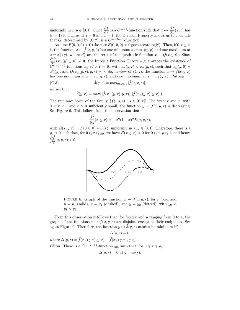
The minimax norm of the family {f(·, s, r) | s ∈ [0, r]}. For fixed x and r, with

0 < x < 1 and r > 0 sufficiently small, the function y 7→ f(x, y, r) is decreasing.See Figure 6. This follows from the observation that

∂f

∂y(x, y, r) = −xn(1 − x)nE(x, y, r),

with E(x, y, r) = F (0, 0, 0) + O(r), uniformly in x, y ∈ [0, 1]. Therefore, there is a0 > 0 such that, for 0 6 r 6 0, we have E(x, y, r) > 0 for 0 6 x, y 6 1, and hence

∂f∂y

(x, y, r) < 0.

0.2 0.4 0.6 0.8 1

Figure 6. Graph of the function x 7→ f(x, y, r), for r fixed andy = y0 (solid), y = y1 (dashed), and y = y2 (dotted), with y0 <

y1 < y2.

From this observation it follows that, for fixed r and y ranging from 0 to 1, thegraphs of the functions x 7→ f(x, y, r) are disjoint, except at their endpoints. See

again Figure 6. Therefore, the function y 7→ δ(y, r) attains its minimum iff

∆(y, r) = 0,

where ∆(y, r) = f(x−(y, r), y, r) + f(x+(y, r), y, r).

Claim: There is a Cm−2n+1-function y0, such that, for 0 6 r 6 0:

∆(y, r) = 0 iff y = y0(r).


and y0(r) = 12 + O(r).

To prove this claim, we first prove that ∆(12 , 0) = 0. To see this, observe that

f(x, 12 , 0) = −f(1 − x, 1

2 , 0),

so∂f

∂x(x, 1

2 , 0) =∂f

∂x(1 − x, 1

2 , 0).

Therefore, x+(12 , 0) = 1 − x−(1

2 , 0), and hence ∆(12 , 0) = 0. Since

∂∆

∂y(y, 0) =

∂f

∂y(x−(y, 0), y, 0) +

∂f

∂y(x+(y, 0), y, 0) < 0,

the function y 7→ ∆(y, 0) has a unique zero at y = 12 . Furthermore, the Im-

plicit Function Theorem guarantees the existence of a Cm−2n+1-function y0 with∆(y0(r), r) = 0, and y0(0) = 1

2 .In view of (C.3) we have

min06y61 δ(y, r) = |f(x±(y0(r), r), y0(r), r)|= |f(x±(1

2 , 0), 12 , 0)| +O(r)

= max06x61 |xn(1 − x)n(x − 12 )| +O(r)

= cn +O(r).

Finally, min06s6r δ(s, r) = r2n+1 min06y61 δ(y, r) = cn r2n+1 + O(r2n+2). The

minimum is attained at s = s0(r) = r y0(r). Obviously, s0 is a Cm−2n+1-function.This concludes the proof of the second part of the Lemma. �

References

[1] Y.J. Ahn. Conic approximation of planar curves. Computer-Aided Design, 33(12):867–872,2001.

[2] E. Berberich, A. Eigenwillig, M. Hemmer, S. Hert, K. Mehlhorn, and E. Schmer. A compu-tational basis for conic arcs and Boolean operations on conic polygons. In Proc. of European

Symposium on Algorithms, volume 2461 of Lecture Notes in Computer Science, pages 174–186, 2002.

[3] W. Blaschke. Vorlesungen uber Differentialgeometrie II. Affine Differential Geometrie, vol-ume VII of Die Grundlehren der mathematischen Wissenschaften in Einzeldarstellungen.Springer-Verlag, 1923.

[4] B.D. Bojanov, H.A. Hapokian, and A.A. Sahakian. Spline functions and multivariate in-

terpolation, volume 248 of Mathematics and its Applications. Kluwer Academic Publishers,Dordrecht, 1993.

[5] C. de Boor, K. Hollig, and M. Sabin. High accuracy geometric Hermite interpolation. Com-

puter Aided Geometric Design, 4:269–278, 1987.[6] W.L.F. Degen. Geometric Hermite interpolation – in memoriam Josef Hoschek. Computer

Aided Geometric Design, 22:573–592, 2005.[7] R.A. DeVore and G.G. Lorentz. Constructive Approximation, volume 303 of Grundlehren der

mathematischen Wissenschaften. Springer-Verlag, Berlin, 1993.[8] T. Dokken. Approximate implicitization. In T. Lyche and L.L. Schumaker, editors, Math-

ematical Methods in CAGD: Oslo 2000, Innovations In Applied Mathematics Series, pages81–102. Vanderbilt University Press, 2001.

[9] T. Dokken and J.B. Thomassen. Overview of approximate implicitization. In R. Goldman

and R. Krasauskas, editors, Topics in Algebraic Geometry and Geometric Modelling, volume334 of Series on Contemporary Mathematics, pages 169–184. AMS, 2003.

[10] I. Emiris, E. Tsigaridas, and G. Tzoumas. The predicates for the Voronoi diagram of ellipses.In Proc. of ACM Symp. Comput. Geom., pages 227–236, 2006.


[11] I. Emiris and G. Tzoumas. A real-time and exact implementation of the predicates for theVoronoi diagram of parametric ellipses. In Proc. of ACM Symp. Solid Physical Modeling,

China, 2007. To appear.[12] G. Farin. Curvature continuity and offsets for piecewise conics. ACM Trans. Graphics,

8(2):89–99, 1989.[13] L. Fejes Toth. Approximations by polygons and polyhedra. Bull. Amer. Math. Soc., 54:431–

438, 1948.[14] M.S. Floater. An O(h2n) Hermite approximation for conic sections. Computer Aided Geo-

metric Design, 14:135–151, 1997.[15] M. Li, X.-S. Gao, and S.-C. Chou. Quadratic approximation to plane parametric curves and

its application in approximate implicitization. Visual Computer, 22:906–917, 2006.[16] M. Ludwig. Asymptotic approximation of convex curves. Arch. Math., 63:377–384, 1994.[17] M. Ludwig. Asymptotic approximation of convex curves; the Hausdorff metric case. Arch.

Math., 70:331–336, 1998.[18] M. Ludwig. Asymptotic approximation by quadratic spline curves. Ann. Univ. Sci. Budapest,

Sectio Math., 42:133–139, 1999.[19] D.E. McClure and R.A. Vitale. Polygonal approximation of plane convex bodies. J. Math.

Anal. Appl., 51:326–358, 1975.[20] C.A. Micchelli. On a numerically efficient method for computing multivariate B-splines. In

Multivariate Approximation Theory, volume 51 of ISNM, pages 211–248. Birkhauser Verlag,1979.

[21] N. Norlund. Vorlesungen uber Differenzenrechnung, volume XIII of Grundlehren der Math-

ematischen Wissenschaften. Springer-Verlag, Berlin, 1924.[22] P.J. Olver, G. Sapiro, and A. Tannenbaum. Affine invariant detection: edge maps, anisotropic

diffusion, and active contours. Acta Appl. Math., 59:45–77, 1999.[23] V. Ovsienko and S. Tabachnikov. Projective Differential Geometry Old and New. From the

Schwarzian Derivative to the Cohomology of Diffeomorphism Groups, volume 165 of Cam-

bridge Tracts in Mathematics. Cambridge University Press, 2005.[24] H. Pottmann. Locally controllable conic splines with curvature continuity. ACM Trans.

Graphics, 10(4):366–377, 1991.[25] M.J.D. Powell. Approximation Theory and Methods. Cambridge University Press, Cambridge,

1981.[26] R. Schaback. Planar curve interpolation by piecewise conics of arbitrary type. Constructive

Approximation, 9:373–389, 1993.[27] S. Tabachnikov and V. Timorin. Variations on the Tait-Kneser theorem. Technical report,

Department of Mathematics. Pennsylvania State University., 2006.[28] X. Yang. Curve fitting and fairing using conic splines. Computer-Aided Design, 36(5):461–472,

2004.

University of Groningen, The Netherlands

E-mail address: [email protected]

LORIA-CNRS, Nancy, France


University of Groningen, The Netherlands


Sunayana Ghosh, Sylvain Petitjean, Gert Vegter To cite ... · Approximation by conic splines Sunayana Ghosh, ... among all such bitangent conics. ... Paper overview. Section 2 reviews

Documents