Welcome message from author
This document is posted to help you gain knowledge. Please leave a comment to let me know what you think about it! Share it to your friends and learn new things together.
Transcript

2 Quantifcation Methodologies
Alberta Environment and Parks
February 2020
Quantification Methodologies for the Carbon Competitiveness Incentive Regulation and the Specified Gas Reporting Regulation

3 Quantifcation Methodologies
Summary of Revisions Version Date Summary of Revisions
1.0 June 2018 First publication of chapters 1, 8, 12, 13, 14, and 17 and Appendix A,
B, C, and D.
1.1 November 2018 Revision 1 to chapters 1, 8, 12, 13, 14, and 17 and Appendix A, B, C,
and D.
Updates and corrections to emission factors in Chapter 1 (Tables
1-1 to 1-4).
Added technology based emission factors for methane and
nitrous oxide in Chapter 1 (Table 1-3).
Updates to the structure of methods and tier classification in
Chapter 1 (Figures 1-1 and 1-2).
New methods introduced in Chapter 8 (Section 8.2.5) and
Appendix C (Section C.6).
Updates to fuel properties in Appendix B.
Updates to production in Chapter 13 to include ethylene glycol
and high value chemicals (HVC).
Updates to Section 17.3 in Chapter 17.
Other minor miscellaneous edits to various chapters.
1.2 November 2019 First publication of chapters 4 and 5.
1.3 January 2020 The following updates were made to chapters 1, 5, 8, 12, 13, 14, and
17:
Minor updates and corrections throughout the chapters.
Clarification on fuel used for flare pilot.
Definition of negligible emissions sources.
Emission factors in chapters 1 and 14.
Quantification methodologies for lime kilns in Kraft pulp mills in
chapter 8.
Alberta Gas Processing Index (ABGPI) in chapter 13.
Fuel consumption requirements in chapter 17.
Table 17.3 to provide clarity on sampling frequencies.

4 Quantifcation Methodologies
Table of Contents
Summary of Revisions ................................................................................................................... 3
Introduction ..................................................................................................................................... 7
Scope and Applicability ................................................................................................................ 7
Activity Type ................................................................................................................................. 8
Application for Deviation Requests .............................................................................................. 9
Definitions .................................................................................................................................... 9
1.0 Quantification Methods for Stationary Fuel Combustion......................................... 13
1.1 Introduction .......................................................................................................................... 13
1.2 Carbon Dioxide .................................................................................................................... 13
1.3 Methane and Nitrous Oxide ................................................................................................. 20
1.4 Emission factors ................................................................................................................... 23
4.0 Quantification of Venting Emissions ......................................................................... 30
4.1 General Calculation ............................................................................................................. 31
4.2 Routine Venting–Produced Gas at UOG Facilities .............................................................. 36
4.3 Routine Venting-Continuous Gas Analyzer Purge .............................................................. 39
4.4 Routine Venting-Solid Desiccant Dehydrators ..................................................................... 40
4.5 Routine Venting-Pigging and Purges ................................................................................... 42
4.6 Routine Venting-Atmospheric Liquid Storage Tank ............................................................. 46
4.7 Routine Venting-Pneumatic Control Instruments ................................................................. 63
4.8 Routine Venting-Pneumatic Pumps ..................................................................................... 76
4.9 Compressor Seal Venting .................................................................................................... 85
4.10 Glycol Dehydrator Venting ................................................................................................. 91
4.11 Glycol Refrigeration Venting .............................................................................................. 93
4.12 Acid Gas Removal (AGR)/Sulphur Recovery Units Venting .............................................. 93
4.13 Hydrocarbon Liquid Loading/Unloading Venting ............................................................... 96
4.14 Oil-Water Separator Venting for Refineries ..................................................................... 100
4.15 Produced Water Tank Venting ......................................................................................... 103
4.16 Non-Routine Venting-Well Tests, Completion, and Workovers ....................................... 105
4.17 Non-Routine Venting-Process System Blowdown ........................................................... 106
4.18 Non-Routine Venting-Gas Well Liquids Unloading .......................................................... 107
5 Quantifcation Methodologies
4.19 Non-Routine Venting-Engine and Turbine Starts ............................................................ 111
4.20 Non-Routine Venting-Pressure Relief .............................................................................. 128
4.21 Other Venting Emission Sources ..................................................................................... 129
5.0 Quantification Methods for On-Site Transportation .............................................. 131
5.1 Introduction ........................................................................................................................ 131
5.2 Carbon Dioxide .................................................................................................................. 132
5.3 Methane and Nitrous Oxide ............................................................................................... 133
8.0 Quantification of Industrial Process Emissions ..................................................... 137
8.1 Introduction ........................................................................................................................ 137
8.2 CO2 from hydrogen production .......................................................................................... 138
8.3 CO2 from calcining carbonates (minerals) ......................................................................... 148
8.4 CO2 from use of carbonates .............................................................................................. 155
8.5 CO2 from ethylene oxide production .................................................................................. 159
8.6 CO2 from use of carbon as reductant ................................................................................. 161
8.7 N2O from nitric acid production .......................................................................................... 162
8.8 CO2 from thermal carbon black production ........................................................................ 170
12.0 Quantification of Imports ................................................................................................... 173
12.1 Introduction ...................................................................................................................... 173
12.2 Imported Useful Thermal Energy ..................................................................................... 173
12.3 Imported Electricity .......................................................................................................... 174
12.4 Imported Hydrogen .......................................................................................................... 174
13.0 Quantification of Production ............................................................................................. 175
13.1 Introduction ...................................................................................................................... 175
13.2 Ammonia .......................................................................................................................... 176
13.3 Ammonium Nitrate ........................................................................................................... 176
13.4 Bituminous Coal ............................................................................................................... 176
13.5 Cement ............................................................................................................................. 177
13.6 Electricity .......................................................................................................................... 177
13.7 Ethylene Glycol ................................................................................................................ 177
13.8 Hardwood Kraft Pulp ........................................................................................................ 177
13.9 High Value Chemicals ...................................................................................................... 177
13.10 Hydrogen........................................................................................................................ 177
13.11 Industrial Heat ................................................................................................................ 178
13.12 Oil Sands In Situ Bitumen .............................................................................................. 178
13.13 Oil Sands Mining Bitumen .............................................................................................. 178

6 Quantifcation Methodologies
13.14 Refining .......................................................................................................................... 178
13.15 Softwood Kraft Pulp ................................................................................................. 187
13.16 Alberta Gas Processing Index ....................................................................................... 187
14.0 Quantification Methods for Carbon Dioxide from Combustion of Biomass ................ 196
14.1 Introduction ...................................................................................................................... 196
14.2 Tier 1 - A fuel-specific default CO2 emission factor ......................................................... 196
14.3 Tier 2 - Place marker. ...................................................................................................... 197
14.4 Tier 3 - Measurement of fuel carbon content ................................................................... 197
14.5 Tier 4 Continuous emissions monitoring systems ........................................................... 200
14.6 Emission Factors ............................................................................................................. 203
17.0 Measurement, Sampling, Analysis and Data Management Requirements ................... 204
17.1 Introduction ...................................................................................................................... 204
17.2 Fuel consumption ............................................................................................................. 204
17.3 Equipment, fuel and properties sampling frequency ....................................................... 209
17.4 Data analysis and data management .............................................................................. 211
APPENDIX A: References ....................................................................................................... 215
APPENDIX B: Fuel Properties ................................................................................................... 216
APPENDIX C: General Calculation Instructions ...................................................................... 218
APPENDIX D: Conversion Factors............................................................................................ 228
APPENDIX E: Alberta Gas Processing Index .......................................................................... 232
7 Quantifcation Methodologies
Introduction The Carbon Competitiveness Incentive Regulation (CCIR) and the Specified Gas Reporting
Regulation (SGRR) require the use of standard quantification methods for the reporting of
greenhouse gas emissions under each respective regulation. The Quantification Methodologies
for the CCIR and SGRR provides the standard methods for activities that generate greenhouse
gas emissions. Some methods prescribed in this document are only applicable to one of the
regulations and the reporting of emissions and other parameters such as production and biomass
emissions must follow the requirements under the respective regulation. Where quantification
methods and emission factors are not prescribed or if deviations from prescribed methods are
required, alternative methods may be proposed by the reporter and will be reviewed and
approved by the Director on a case-by-case basis. Procedures to request for deviations and/or
alternative methods are described in the Standard for Completing Greenhouse Gas Compliance
and Forecasting Reports for regulated facilities under CCIR.
For some activities, several methods are outlined to quantify greenhouse gas emissions, which
may include mass balances, emission factors, engineering estimates, and/or direct emissions
measurements. These methods have been identified as “tiers” of quantification methods. The
Specified Gas Reporting Standard and the Standard for Completing Greenhouse Gas
Compliance and Forecasting Reports prescribes the “tier” method that is required for a facility that
is reporting under SGRR and/or CCIR respectively.
The Quantification Methodologies for the CCIR and SGRR, the Specified Gas Reporting
Standard, and the Standard for Completing Greenhouse Gas Compliance and Forecasting
Reports will be updated from time to time. Regulated facilities are required to use the most up-to-
date version of these documents in the reporting of greenhouse gas emissions under the
respective regulations.
Scope and Applicability
The objective of the quantification methodologies is to ensure accuracy and consistency across
reporters and sectors regulated under the CCIR and SGRR. The intention is also to align with
methods that are prescribed by Environment and Climate Change Canada (ECCC) and other
jurisdictions that regulate greenhouse gas emissions such as British Columbia, Ontario, Quebec,
and California. Further, methodologies from organizations such as the Western Climate Initiative,
Inc. (WCI) and the Intergovernmental Panel on Climate Change (IPCC) are referenced or
adopted as appropriate for various activity types and modified to meet the needs of Alberta
sectors.

8 Quantifcation Methodologies
Greenhouse gas emissions covered in these quantification methods include carbon dioxide
(CO2), methane (CH4), nitrous oxide (N2O), sulphur hexafluoride (SF6), nitrogen trifluoride (NF3),
hydrofluorocarbons (HFCs), and perfluorocarbons (PFCs). For a complete list of HFCs and PFCs,
refer to the Standard for Completing Greenhouse Gas Compliance and Forecasting Reports.
For some reporting purposes facilities are required to apply the appropriate Global Warming
Potential (GWPs) to the greenhouse gas in order to calculate the carbon dioxide equivalent
(CO2e). These GWPs are prescribed in the standards corresponding to the respective
regulations.
Activity Type
This Quantification Methodologies for the CCIR and SGRR provides quantification methods for
the following activities:
Chapter 1: Stationary Fuel Combustion
Chapter 2: Flaring
Chapter 3: Fugitives
Chapter 4: Venting
Chapter 5: On-Site Transportation
Chapter 6: Waste and Digestion
Chapter 7: Wastewater
Chapter 8: Industrial Processes
Chapter 9: HFCs, PFCs, SF6, NF3
Chapter 10: Formation CO2
Chapter 11: Injected, Sent Offsite, Received CO2
Chapter 12: Imports
Chapter 13: Production
Chapter 14: Carbon Dioxide Emissions from Combustion of Biomass
Chapter 15: Reporting Requirements under CCIR and SGRR
9 Quantifcation Methodologies
The chapters below provide guidance for reporters:
Chapter 17: Measuring, Sampling, Analysis and Data Management
The following appendices provide support to the activities presented in the above chapters:
Appendix A: References
Appendix B: Fuel Properties
Appendix C: General Calculation Instructions
Appendix D: Conversion Factors
Application for Deviation Requests
Facilities that are unable to execute a prescribed method must request a time limited approval to
deviate from the prescribed method. The application should include:
A description of the alternative method to be used
Evidence that the alternative method would tend to be conservative versus the prescribed
method
A plan for future adoption of the prescribed method
The Director will review the request to deviate and issue a letter indicating whether it is approved.
This letter should be kept as record to support verification activities. For further information on this
process please consult the Standard for Completing Greenhouse Gas Compliance and
Forecasting Reports for regulated facilities under CCIR.
Definitions
“AB-CWB Methodology” means the methodology based on CAN-CWB and adapted to Alberta
framework.
“Accuracy” means the ability of a measurement instrument to indicate values closely
approximating the true value of the quantity measured.
“bbl/cd”” means barrels per calendar day.
“Bias” means any influence on a result that produces an incorrect approximation of the true value
of the variable being measured. Bias is the result of a predictable systematic error.
10 Quantifcation Methodologies
“Biomass” means organic matter consisting of, or recently derived from living organisms.
“Biogenic emissions” are derived from biomass, either through combustion or other processes.
“Calibration” means the process or procedure of adjusting an instrument so that its indication or
registration is in satisfactorily close agreement with a reference standard.
“CAN-CWB Methodology” means the calculation methodology described in “The CAN-CWB
Methodology for Regulatory Support: Public Report” dated January 2014, prepared by Solomon
Associates.
“Carbon content” means the fraction of carbon in the material.
“Consensus Based Standards Organization” means ASTM International, the American Gas
Association (AGA), the American Petroleum Institute (API), the CSA Group, the Gas Processors
Association (GPA),the Canadian General Standards Board, the Gas Processors Suppliers
Association (GPSA), the American National Standards Institute (ANSI), the American Society of
Mechanical Engineers (ASME), the American Petroleum Institute (API), and the North American
Energy Standards Board (NAESB), International Organization for Standardization (ISO), British
Standard Institution, Measurement Canada, or other similar standards organizations.
“Compensation” means the adjustment of the measured value to reference conditions (e.g.
pressure compensation).
“Continuous emission monitoring system (CEMS)” means the equipment required to sample,
analyze, measure, and provide, by means of monitoring at regular intervals, a record of gas
concentrations, pollutant emission rates, or gas volumetric flow rates from stationary sources.
“Cogeneration unit” means a fuel combustion device which simultaneously generates electricity
and either heat or steam.
“FCC” means Fluid Catalytic Cracker.
“Fuel” means solid, liquid or gaseous combustible material.
“Fuel gas” means typically a mixture of light hydrocarbon and other molecules (e.g. H2, N2) in a
gaseous state that are consumed in fired heaters. Fuel gas is often a mixture of recovered
gaseous molecules from plant operations and purchased natural gas.
“GHGs” means greenhouse gases.
“GWP” means global warming potential.
“HFCs” means hydrofluorocarbons.

11 Quantifcation Methodologies
"Higher Heating Value” or HHV means the amount of heat released by a specified quantity of fuel
once it is combusted and the products have returned to the initial temperature of the fuel, which
takes into account the latent heat of vaporization of water in the combustion products.
“Influence parameter” means any factor that impacts the performance of the measuring device,
hence the uncertainty and accuracy of the measurement. Examples are process temperature,
pressure, fluid composition, upstream straight length, etc.
“Inspection” means a visual assessment or mechanical activity (e.g. instrument lead line blow
down or orifice plate cleanliness) that does not include comparison or adjustment to a reference
standard.
“Instrument Verification” means the process or procedure of comparing an instrument to a
reference standard to ensure its indication or registration is in satisfactorily close agreement,
without making an adjustment.
“Landfill Gas” (LFG) means the mixture of methane and carbon dioxide generated by
decomposing organic waste in Solid Waste Disposal Sites.
"Lower Heating Value” or LHV means the amount of heat released by combusting a specified
quantity of fuel and returning the temperature of the combustion products to 150°C, which
assumes the latent heat of vaporization of water in the reaction products is not recovered.
“Meter condition factor” means an estimate of additional uncertainty based on a technical
judgment of the physical condition of the meter in lieu of the ability to inspect.
“Metering or measurement system” means a combination of primary, secondary and/or tertiary
measurement components necessary to determine the flow rate.
“Municipal waste” is waste collected by municipalities or other local authorities. Typically, MSW
includes: household waste, garden (yard) and park waste and commercial/institutional waste.
“NAICS” is the North American Industry Classification System.
“Negligible emission sources” are sources with emissions that represent less than 1% of a
facility’s total regulated emissions (TRE) or output-based allocation (OBA) (CO2e) and are not to
exceed 5,000 tonne of CO2e for a facility with a TRE less than 1 million tonnes of CO2e or not to
exceed 10,000 tonnes of CO2e for a facility with TRE equal to or greater than 1 million tonnes of
CO2e under CCIR. Alternative methods may be used to assess the negligibility of these
emissions.
“Performance” means the response of a measurement device to influence parameters such as
operating conditions, installation effects, and fluid properties.

12 Quantifcation Methodologies
“Range of uncertainty” means the range or interval within which the true value is expected to lie
with a stated degree of confidence.
“Standard Temperature and Pressure” or “STP conditions" or "standard condition" means
conditions at 15.0 degrees Celsius and 1 atmosphere of absolute pressure.
“Uncertainty” means the description of the range of deviation between a measured value and the
true value, expressed as a percentage. For example, a device with an accuracy of 2% would
have an uncertainty of ±2 %.
“2006 Intergovernmental Panel on Climate Change (IPCC) Guidelines”: 2006 IPCC Guidelines for
National Greenhouse Gas Inventories. Intergovernmental Panel on Climate Change National
Greenhouse Gas Inventories Program. Available online at: http://www.ipcc-
nggip.iges.or.jp/public/2006gl/index.html.
σ means the standard deviation.

13 Quantifcation Methodologies
1.0 Quantification Methods for Stationary Fuel Combustion
1.1 Introduction
Stationary fuel combustion sources are devices that combust solid, liquid, or gaseous fuel,
generally for the purposes of providing useful heat or energy for industrial, commercial, or
institutional use. Methods for carbon dioxide (CO2) emissions from biomass combustion are
provided in Chapter 14, while methods for methane (CH4) and nitrous oxide (N2O) from biomass
combustion are included in this chapter. Stationary fuel combustion sources include, but are not
limited to boilers, simple and combined-cycle combustion turbines, engines, emergency
generators, portable equipment, process heaters, furnaces and any other combustion devices or
system (e.g. blasting for mining purposes). This source category does not include flare emission
sources, except for fuel that is combusted for the flare pilot, or waste incineration, which are
discussed in Chapter 2 and Chapter 6, respectively.
1.2 Carbon Dioxide
1.2.1 Introduction
For each fuel type combusted, calculate the mass of CO2 emissions from fuel combustion for the
reporting period, using one of the four quantification methodologies specified in this section.
Various methods to calculate CO2 emissions from different fuel types are presented in this
section. A facility must use the method that corresponds with the tier classification that is
assigned to the facility as illustrated in Figure 1.1. A facility must also apply the sampling and
measurement requirements in Chapter 17 that corresponds with the facility's tier classification.
Figure 1-1 Tier classification and methodology mapping
Tier Classification
1 2 3 4
Fuel
Types
Non-Variable Method 1
Method 4 Natural Gas Method 2
Variable Method 3

14 Quantifcation Methodologies
1.2.2 Method 1 - A fuel-specific default CO2 emission factor for non-
variable fuels
(1) Introduction
This method is used for fuels that are non-variable in composition and based on a default CO2
emission factor and the quantity of fuel consumed. This method can be used for tiers 1, 2, or 3 as
illustrated in Figure 1-1. Non-variable fuels that are acceptable to be used under this methodology
include ethane, propane, butane, diesel, and gasoline. For diesel and gasoline that is subject to
the Renewable Fuels Standard (RFS), the default CO2 emission factors take into account the
biofuel that is required as part of the fuel composition. Under the RFS, gasoline and diesel must
contain 5% and 2% biofuel, respectively. Note the biofuels are included in the chapter for CO2
from biomass combustion. The quantity of fuel consumed may be measured on a volume or
energy basis, which can be provided by a third party supplier (i.e. invoices) or measured by the
facility using the methods prescribed in Chapter 17 and Appendix C. Fuel consumption measured
or provided in units of energy must be based on the higher heating value (HHV) of the fuel. Table
1-1 provides the emission factors for these fuels in mass of CO2 emitted per gigajoules (GJ) or
kilolitres (kl).
For facilities that have the HHV of the fuel, measured or supplied by the third party supplier,
Equation 1-1 is used to convert the volume of the fuel to the energy of the fuel based on the HHV
and then multiplied by the appropriate energy based emission factor from Table 1-1 to calculate
the CO2 mass emissions. For facilities that have the quantity of fuel in energy basis, Equation 1-
1a can be used directly to calculate the CO2 mass emissions based on the appropriate energy
based emission factor from Table 1-1.
Facilities must use measured or supplied HHVs to determine the fuel consumption if this data is
available; however in cases where a facility is unable to obtain this information, a facility may
apply Equation 1-1a using the fuel quantity in volume basis with the appropriate volume based
emission factor from Table 1-1 to calculate the CO2 mass emissions.
(2) Equations
For a liquid or gaseous fuel, use Equation 1-1 or Equation 1-1a to calculate the CO2 mass
emissions for the reporting period.
𝑪𝑶𝟐,𝒑 = 𝝊𝒇𝒖𝒆𝒍,𝒑 × 𝑯𝑯𝑽 × 𝑬𝑭𝒆𝒏𝒆 Equation 1-1
𝑪𝑶𝟐,𝒑 = 𝝊𝒇𝒖𝒆𝒍,𝒑 × 𝑬𝑭𝒗𝒐𝒍 𝒐𝒓 𝑬𝑵𝑬𝒇𝒖𝒆𝒍,𝒑 × 𝑬𝑭𝒆𝒏𝒆 Equation 1-1a
15 Quantifcation Methodologies
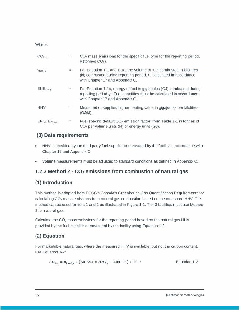
Where:
CO2, p = CO2 mass emissions for the specific fuel type for the reporting period,
p (tonnes CO2).
νfuel, p = For Equation 1-1 and 1-1a, the volume of fuel combusted in kilolitres
(kl) combusted during reporting period, p, calculated in accordance
with Chapter 17 and Appendix C.
ENEfuel,p = For Equation 1-1a, energy of fuel in gigajoules (GJ) combusted during
reporting period, p. Fuel quantities must be calculated in accordance
with Chapter 17 and Appendix C.
HHV = Measured or supplied higher heating value in gigajoules per kilolitres
(GJ/kl).
EFvol, EFene = Fuel-specific default CO2 emission factor, from Table 1-1 in tonnes of
CO2 per volume units (kl) or energy units (GJ).
(3) Data requirements
HHV is provided by the third party fuel supplier or measured by the facility in accordance with
Chapter 17 and Appendix C.
Volume measurements must be adjusted to standard conditions as defined in Appendix C.
1.2.3 Method 2 - CO2 emissions from combustion of natural gas
(1) Introduction
This method is adapted from ECCC's Canada's Greenhouse Gas Quantification Requirements for
calculating CO2 mass emissions from natural gas combustion based on the measured HHV. This
method can be used for tiers 1 and 2 as illustrated in Figure 1-1. Tier 3 facilities must use Method
3 for natural gas.
Calculate the CO2 mass emissions for the reporting period based on the natural gas HHV
provided by the fuel supplier or measured by the facility using Equation 1-2.
(2) Equation
For marketable natural gas, where the measured HHV is available, but not the carbon content,
use Equation 1-2:
𝑪𝑶𝟐,𝒑 = 𝝊𝒇𝒖𝒆𝒍,𝒑 × (𝟔𝟎. 𝟓𝟓𝟒 × 𝑯𝑯𝑽𝒑 − 𝟒𝟎𝟒. 𝟏𝟓) × 𝟏𝟎−𝟔 Equation 1-2

16 Quantifcation Methodologies
Where:
CO2, p = CO2 mass emissions for the marketable natural gas combusted during
the reporting period, p (tonnes CO2).
νfuel, p = Volume of fuel (m3) at standard conditions combusted during reporting
period, p, calculated in accordance with Chapter 17 and Appendix C.
HHVp = Weighted average measured higher heating value of fuel (MJ/m3) at
standard conditions as defined in Appendix C.
(60.554 × HHVp
- 404.15)
= Empirical equation adapted from ECCC (grams of CO2 per cubic meter
of natural gas) representing relationship between CO2 and volume of
natural gas determined through higher heating value using a discreet
set of data collected by ECCC.
10-6 = Mass conversion factor (t/g).
(3) Data requirements
HHV is provided by the third party fuel supplier or measured by the facility in accordance with
Chapter 17 and Appendix C.
Volume measurements must be adjusted to standard conditions as defined in Appendix C.
1.2.4 Method 3 - CO2 emissions from variable fuels based on the
measured fuel carbon content
(1) Introduction
This method is used for variable fuels based on a mass balance approach using the measured
fuel carbon content. This method can be used for tiers 1, 2, or 3. Variable fuels are those that
have varying composition and require testing for carbon content. All fuels not listed as non-
variable fuels are to be considered variable fuels. The quantity of fuel consumed and/or the
carbon content may be provided by the third party supplier (i.e. invoices or third party
documentation) or measured by the facility using the methods prescribed in Chapter 17 and
Appendix C.
For FCC processes, the emissions are considered to be stationary fuel combustion; however,
there are no quantification methodologies currently prescribed. Facilities performing these

17 Quantifcation Methodologies
processes may develop their own quantification methodologies or apply existing quantification
methodologies until such methodologies are provided in this chapter.
Calculate the CO2 mass emissions for the reporting period for each fuel based on Equation 1-3a,
Equation 1-3b, Equation 1-3c, or Equation 1-3d depending on the type of fuel combusted.
(2) Equations
For gaseous fuels, where fuel consumption is measured in units of volume (m3), use Equation 1-
3a:
𝑪𝑶𝟐,𝒑 = 𝝂𝒇𝒖𝒆𝒍 (𝒈𝒂𝒔),𝒑 × 𝑪𝑪𝒈𝒂𝒔,𝒑 × 𝟑. 𝟔𝟔𝟒 × 𝟎. 𝟎𝟎𝟏 Equation 1-3a
For gaseous fuels, where fuel consumption is measured in units of energy (GJ), use Equation 1-
3b:
𝑪𝑶𝟐,𝒑 =𝑬𝑵𝑬𝒇𝒖𝒆𝒍 (𝒈𝒂𝒔),𝒑×𝑪𝑪𝒈𝒂𝒔,𝒑× 𝟑.𝟔𝟔𝟒×𝟎.𝟎𝟎𝟏
𝑯𝑯𝑽 Equation 1-3b
Where:
CO2,p = CO2 mass emissions for the gaseous fuel combusted during the
reporting period, p (tonnes CO2).
νfuel(gas), p = Volume of fuel (m3) at standard conditions combusted during
reporting period, p, calculated in accordance with Chapter 17 and
Appendix C.
ENEfuel(gas),p = Energy of fuel (GJ) at standard conditions combusted during
reporting period, p, calculated in accordance with Chapter 17 and
Appendix C.
HHV = Weighted average higher heating value of fuel (GJ/m3) at standard
conditions as defined in Appendix C.
CCgas,p = Weighted average carbon content of the gaseous fuel during the
reporting period p, calculated in accordance with Chapter 17 and
Appendix C. CCp is in units of kilogram of carbon per standard cubic
metre of gaseous fuel (kg C/m3).
3.664 = Ratio of molecular weights, CO2 to carbon.

18 Quantifcation Methodologies
0.001 = Mass conversion factor (t/kg).
For a liquid fuel, where fuel consumption is measured in units of volume (kilolitres), use Equation
1-3c:
𝑪𝑶𝟐,𝒑 = 𝝊𝒇𝒖𝒆𝒍(𝒍𝒊𝒒),𝒑 × 𝑪𝑪𝒍𝒊𝒒,𝒑 × 𝟑. 𝟔𝟔𝟒 Equation 1-3c
Where:
CO2,p = CO2 mass emissions for the liquid fuel during the report period, p
(tonnes CO2).
νfuel(liq),p = Volume of liquid fuel combusted during the reporting period p,
calculated in accordance with Chapter 17 and Appendix C (kilolitres).
CCliq,p = Weighted average carbon content of the liquid fuel during the
reporting period p, calculated in accordance with Chapter 17 and
Appendix C. CCp is in units of tonnes of carbon per kilolitre of liquid
fuel (tonnes C/kl).
3.664 = Ratio of molecular weights, CO2 to carbon.
For a solid fuel, where fuel consumption is measured in units of mass (tonnes), use Equation 1-
3d:
𝑪𝑶𝟐,𝒑 = 𝒎𝒇𝒖𝒆𝒍(𝒔𝒐𝒍),𝒑 × 𝑪𝑪𝒔𝒐𝒍,𝒑 × 𝟑. 𝟔𝟔𝟒 Equation 1-3d
Where:
CO2,p = CO2 mass emissions for the solid fuel during the report period, p
mfuel(sol),p = Mass of solid fuel combusted during the reporting period p,
calculated in accordance with Chapter 17 and Appendix C (tonnes).
CCsol,p = Weighted average carbon content of the fuel during the reporting
period p, calculated in accordance with Chapter 17 and Appendix C.
CCp is in units of tonnes of carbon per tonnes of solid fuel (tonnes
C/tonnes).
19 Quantifcation Methodologies
3.664 = Ratio of molecular weights, CO2 to carbon.
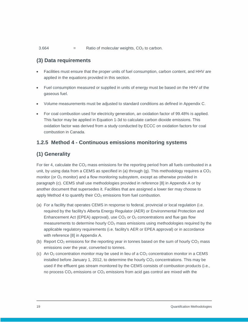
(3) Data requirements
Facilities must ensure that the proper units of fuel consumption, carbon content, and HHV are
applied in the equations provided in this section.
Fuel consumption measured or supplied in units of energy must be based on the HHV of the
gaseous fuel.
Volume measurements must be adjusted to standard conditions as defined in Appendix C.
For coal combustion used for electricity generation, an oxidation factor of 99.48% is applied.
This factor may be applied in Equation 1-3d to calculate carbon dioxide emissions. This
oxidation factor was derived from a study conducted by ECCC on oxidation factors for coal
combustion in Canada.
1.2.5 Method 4 - Continuous emissions monitoring systems
(1) Generality
For tier 4, calculate the CO2 mass emissions for the reporting period from all fuels combusted in a
unit, by using data from a CEMS as specified in (a) through (g). This methodology requires a CO2
monitor (or O2 monitor) and a flow monitoring subsystem, except as otherwise provided in
paragraph (c). CEMS shall use methodologies provided in reference [8] in Appendix A or by
another document that supersedes it. Facilities that are assigned a lower tier may choose to
apply Method 4 to quantify their CO2 emissions from fuel combustion.
(a) For a facility that operates CEMS in response to federal, provincial or local regulation (i.e.
required by the facility's Alberta Energy Regulator (AER) or Environmental Protection and
Enhancement Act (EPEA) approval), use CO2 or O2 concentrations and flue gas flow
measurements to determine hourly CO2 mass emissions using methodologies required by the
applicable regulatory requirements (i.e. facility's AER or EPEA approval) or in accordance
with reference [8] in Appendix A.
(b) Report CO2 emissions for the reporting year in tonnes based on the sum of hourly CO2 mass
emissions over the year, converted to tonnes.
(c) An O2 concentration monitor may be used in lieu of a CO2 concentration monitor in a CEMS
installed before January 1, 2012, to determine the hourly CO2 concentrations. This may be
used if the effluent gas stream monitored by the CEMS consists of combustion products (i.e.,
no process CO2 emissions or CO2 emissions from acid gas control are mixed with the

20 Quantifcation Methodologies
combustion products) and only if the following fuels are combusted in the unit: coal,
petroleum coke, oil, natural gas, propane, butane, wood bark, or wood residue.
(1) If the unit combusts waste-derived fuels (e.g. waste oils, plastics, solvents, dried sewage,
municipal solid waste, tires), emissions calculations shall not be based on O2
concentrations.
(2) If the operator of a facility that combusts biomass fuels uses O2 concentrations to
calculate CO2 concentrations, annual source testing must demonstrate that the
calculated CO2 concentrations, when compared to measured CO2 concentrations, meet
the Relative Accuracy Test Audit (RATA) requirements in reference [8] in Appendix A or
Alberta CEMS Code.
(d) If both biomass and fossil fuels (including fuels that are partially biomass) are combusted
during the year, determine the biomass CO2 mass emissions separately, as described in
Chapter 14.
(e) For any units using CEMS data, industrial process and stationary combustion CO2 emissions
must be provided separately. Determine the quantities of each type of fossil fuel and biomass
fuel consumed for the reporting period, using the fuel sampling approach in Section 17.3 in
Chapter 17.
(f) If a facility subject to requirements for continuous monitoring of gaseous emissions chooses
to add devices to an existing CEMS for the purpose of measuring CO2 concentrations or flue
gas flow, select and operate the added devices using appropriate requirements in
accordance with reference [8] in Appendix A for the facility, as applicable in Alberta under the
Alberta CEMS Code.
(g) If a facility does not have a CEMS and chooses to add one in order to measure CO2
concentrations, select and operate the CEMS using the appropriate requirements in
accordance with reference [8] in Appendix A or equivalent requirements as applicable in
Alberta under the Alberta CEMS Code.
(2) Data requirements
No additional data requirements are needed.
1.3 Methane and Nitrous Oxide
1.3.1 Introduction
Calculate the CH4 and N2O mass emissions for the reporting period from stationary fuel
combustion sources, for each fuel type including biomass fuels, using the methods specified in
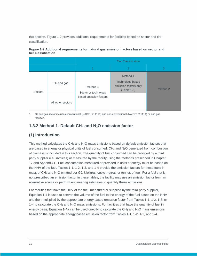
21 Quantifcation Methodologies
this section. Figure 1-2 provides additional requirements for facilities based on sector and tier
classification.
Figure 1-2 Additional requirements for natural gas emission factors based on sector and tier classification
Tier Classification
1 2 3
Sectors
Oil and gas1
Method 1
Sector or technology
based emission factors
Method 1
Technology based
emission factors only
(Table 1-3) Method 2
All other sectors
Oil and gas sector includes conventional (NAICS: 211113) and non-conventional (NAICS: 211114) oil and gas
facilities.
1.3.2 Method 1- Default CH4 and N2O emission factor
(1) Introduction
This method calculates the CH4 and N2O mass emissions based on default emission factors that
are based in energy or physical units of fuel consumed. CH4 and N2O generated from combustion
of biomass is included in this section. The quantity of fuel consumed can be provided by a third
party supplier (i.e. invoices) or measured by the facility using the methods prescribed in Chapter
17 and Appendix C. Fuel consumption measured or provided in units of energy must be based on
the HHV of the fuel. Tables 1-1, 1-2, 1-3, and 1-4 provide the emission factors for these fuels in
mass of CH4 and N2O emitted per GJ, kilolitres, cubic metres, or tonnes of fuel. For a fuel that is
not prescribed an emission factor in these tables, the facility may use an emission factor from an
alternative source or perform engineering estimates to quantify these emissions.
For facilities that have the HHV of the fuel, measured or supplied by the third party supplier,
Equation 1-4 is used to convert the volume of the fuel to the energy of the fuel based on the HHV
and then multiplied by the appropriate energy based emission factor from Tables 1-1, 1-2, 1-3, or
1-4 to calculate the CH4 and N2O mass emissions. For facilities that have the quantity of fuel in
energy basis, Equation 1-4a can be used directly to calculate the CH4 and N2O mass emissions
based on the appropriate energy based emission factor from Tables 1-1, 1-2, 1-3, and 1-4.
22 Quantifcation Methodologies
Facilities must use measured or supplied HHVs to determine the fuel consumption if this data is
available; however in cases where a facility is unable to obtain this information, a facility may
apply Equation 1-4a using the fuel quantity in volume basis with the appropriate volume based
emission factor from Tables 1-1, 1-2, 1-3, or 1-4 to calculated the CH4 and N2O mass emissions.
This method is used for tiers 1, 2, and 3. Figure 1-2 provides additional requirements for natural
gas emission factors based on the sector and tier classification for the facility.
(2) Equations
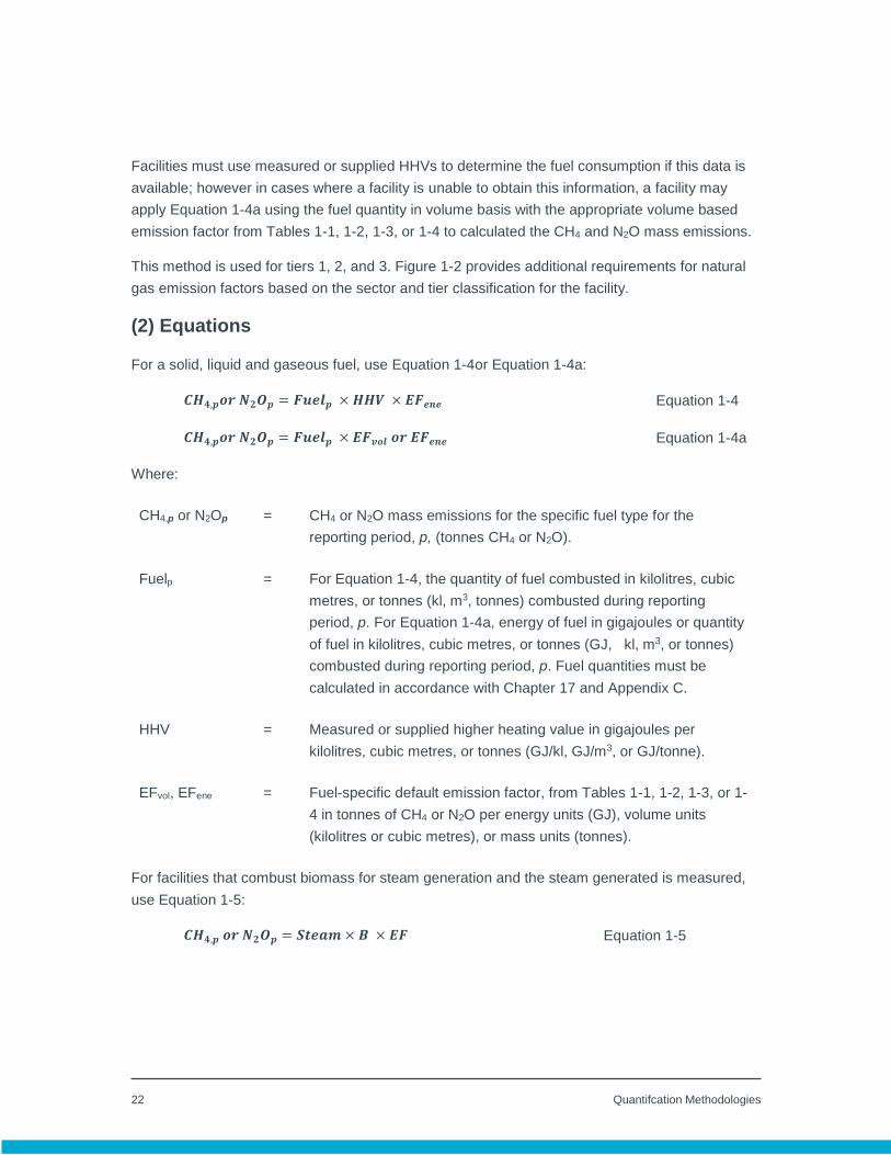
For a solid, liquid and gaseous fuel, use Equation 1-4or Equation 1-4a:
𝑪𝑯𝟒,𝒑𝒐𝒓 𝑵𝟐𝑶𝒑 = 𝑭𝒖𝒆𝒍𝒑 × 𝑯𝑯𝑽 × 𝑬𝑭𝒆𝒏𝒆 Equation 1-4
𝑪𝑯𝟒,𝒑𝒐𝒓 𝑵𝟐𝑶𝒑 = 𝑭𝒖𝒆𝒍𝒑 × 𝑬𝑭𝒗𝒐𝒍 𝒐𝒓 𝑬𝑭𝒆𝒏𝒆 Equation 1-4a
Where:
CH4,p or N2Op = CH4 or N2O mass emissions for the specific fuel type for the
reporting period, p, (tonnes CH4 or N2O).
Fuelp = For Equation 1-4, the quantity of fuel combusted in kilolitres, cubic
metres, or tonnes (kl, m3, tonnes) combusted during reporting
period, p. For Equation 1-4a, energy of fuel in gigajoules or quantity
of fuel in kilolitres, cubic metres, or tonnes (GJ, kl, m3, or tonnes)
combusted during reporting period, p. Fuel quantities must be
calculated in accordance with Chapter 17 and Appendix C.
HHV = Measured or supplied higher heating value in gigajoules per
kilolitres, cubic metres, or tonnes (GJ/kl, GJ/m3, or GJ/tonne).
EFvol, EFene = Fuel-specific default emission factor, from Tables 1-1, 1-2, 1-3, or 1-
4 in tonnes of CH4 or N2O per energy units (GJ), volume units
(kilolitres or cubic metres), or mass units (tonnes).
For facilities that combust biomass for steam generation and the steam generated is measured,
use Equation 1-5:
𝑪𝑯𝟒,𝒑 𝒐𝒓 𝑵𝟐𝑶𝒑 = 𝑺𝒕𝒆𝒂𝒎 × 𝑩 × 𝑬𝑭 Equation 1-5

23 Quantifcation Methodologies
Where:
CH4,p or N2Op CH4 and N2O mass emissions for the specific fuel type for the
reporting period, p (tonnes CH4 or N2O).
Steam Total steam generated by biomass fuel or biomass combustion
during the reporting period (tonnes steam), in GJ and calculated in
accordance with Chapter 17 and Appendix C.
B Ratio of the boiler’s design rated heat input capacity to its design
rated steam output capacity in GJ per GJ calculated in accordance
with Chapter 17.
EF Fuel-specific default CH4 and N2O emission factor, from Table 1-4,
in tonnes of CH4 and N2O per GJ.
(3) Data requirements
HHV is provided by the third party fuel supplier or measured by the facility in accordance with
Chapter 17 and Appendix C.
Facilities that use internal combustion engines are required to use technology based
emission factors for internal combustion engines to calculate the CH4 and N2O emissions
from those equipment.
1.3.3 Method 2 – Continuous emissions monitoring systems
(1) Introduction
The CH4 or N2O emissions for the reporting period attributable to the combustion of any type of
fuel used in stationary combustion units may be calculated using data from CEMS including a gas
volumetric flow rate monitor and a CH4 or N2O concentration monitor, in accordance with
reference [9] in Appendix A or in accordance with the manufacturer’s specifications.
1.4 Emission factors
The tables in this section provide the emission factors to be used in the equations outlined in the
above sections.

24 Quantifcation Methodologies
Table 1-1 Default emission factors by fuel type for non-variable fuels
Non-Variable Fuels HHV
(GJ/kl)1
CO2 Emission Factor4
tonne/kl tonne/GJ
CH4 Emission Factor4
tonne/kl tonne/GJ
N2O Emission Factor4
tonne/kl tonne/GJ
Diesel2 38.35 2.681 0.0699 - - - -
<19kW - - - 7.3E-05 1.9E-06 2.0E-05 5.8E-07
>=19kW, Tier 1-3 - - - 7.3E-05 1.9E-06 2.0E-05 5.8E-07
>=19kW, Tier 4 - - - 7.3E-05 1.9E-06 2.3E-04 5.9E-06
Diesel in Alberta3 37.83 2.610 0.06953 see note 5
Biodiesel6 35.16 - - see note 5
Gasoline
33.43 2.307 0.069
- - - -
2-stroke 1.1E-02 3.0E-04 1.3E-05 3.6E-07
4-stroke 5.1E-03 1.5E-04 6.4E-05 1.8E-06
Gasoline in Alberta3 33.24 2.174 0.06540 see note 7
Butane 28.45 1.747 0.0614 2.4E-05 8.4E-07 1.08E-04 3.8E-06
Ethane 17.21 0.986 0.0573 2.4E-05 1.4E-06 1.08E-04 6.3E-06
Propane 25.29 1.515 0.0599 2.4E-05 9.5E-07 1.08E-04 4.3E-06
For facilities that are unable to obtain the HHV of their fuel, this column presents the default HHV for the non-variable
fuels.
Tiers adapted from USEPA requirements.
Fuels that are impacted by Alberta's Renewable Fuels Standard, where gasoline and diesel emission factors are
adjusted to account for required biofuel content.
Emission factors adapted from ECCC Canada's Greenhouse Gas Quantification Requirements (Reference [3] in
Appendix A).
Diesel CH4 and N2O emission factors are used.
Biodiesel CO2 emission factors are provided in Table 14-1.
Gasoline CH4 and N2O emission factors are used.

25 Quantifcation Methodologies
Table 1-2 Sector based default CH4 and N2O emission factors for natural gas
Natural Gas1 CH4 Emission Factor2
tonne/m3 tonne/GJ
N2O Emission Factor2
tonne/m3 tonne/GJ
Electric Utilities 4.9E-07 1.3E-05 4.9E-08 1.3E-06
Industrial 3.7E-08 9.8E-07 3.3E-08 8.7E-07
Oil and Gas Sector and
Producer Consumption
(Non-marketable)1
3.7E-08 9.8E-07 3.5E-08 9.0E-07
Pipelines 1.9E-06 5.0E-05 5.0E-08 1.3E-06
Cement 3.7E-08 9.8E-07 3.4E-08 9.0E-07
Manufacturing Industries 3.7E-08 9.8E-07 3.3E-08 8.7E-07
Residential, Construction,
Commercial/Institutional,
Agriculture/Other
3.7E-08 9.8E-07 3.5E-08 9.0E-07
Marketable gas is considered to be gas that is saleable for consumption.
Emission factors adapted from ECCC Canada's Greenhouse Gas Quantification Requirements
(Reference [3] in Appendix A).
Table 1-3 Technology based default CH4 and N2O emission factors for natural gas
Natural Gas CH4 Emission Factor
tonne/m3 tonne/GJ
N2O Emission Factor
tonne/m3 tonne/GJ
Reference1
Boilers/Furnaces/Heaters:
NOx Controlled 3.7E-08 9.7E-07 1.0E-08 2.7E-07 AP-42 Table 1.4-2
NOx Uncontrolled 3.7E-08 9.7E-07 3.5E-08 9.3E-07 AP-42 Table 1.4-2
Internal Combustion Engine3:
Turbine 1.4E-07 3.7E-06 4.9E-08 1.3E-06 AP-42 Table 3.1-2a
2 stroke lean 2.37E-05 6.23E-04 AP-42 Table 3.2-1
NOx 90-105% Load - - 7.77E-07 2.04E-05 AP-42 Table 3.2-1
NOx < 90% Load - - 4.75E-07 1.25E-05 AP-42 Table 3.2-1
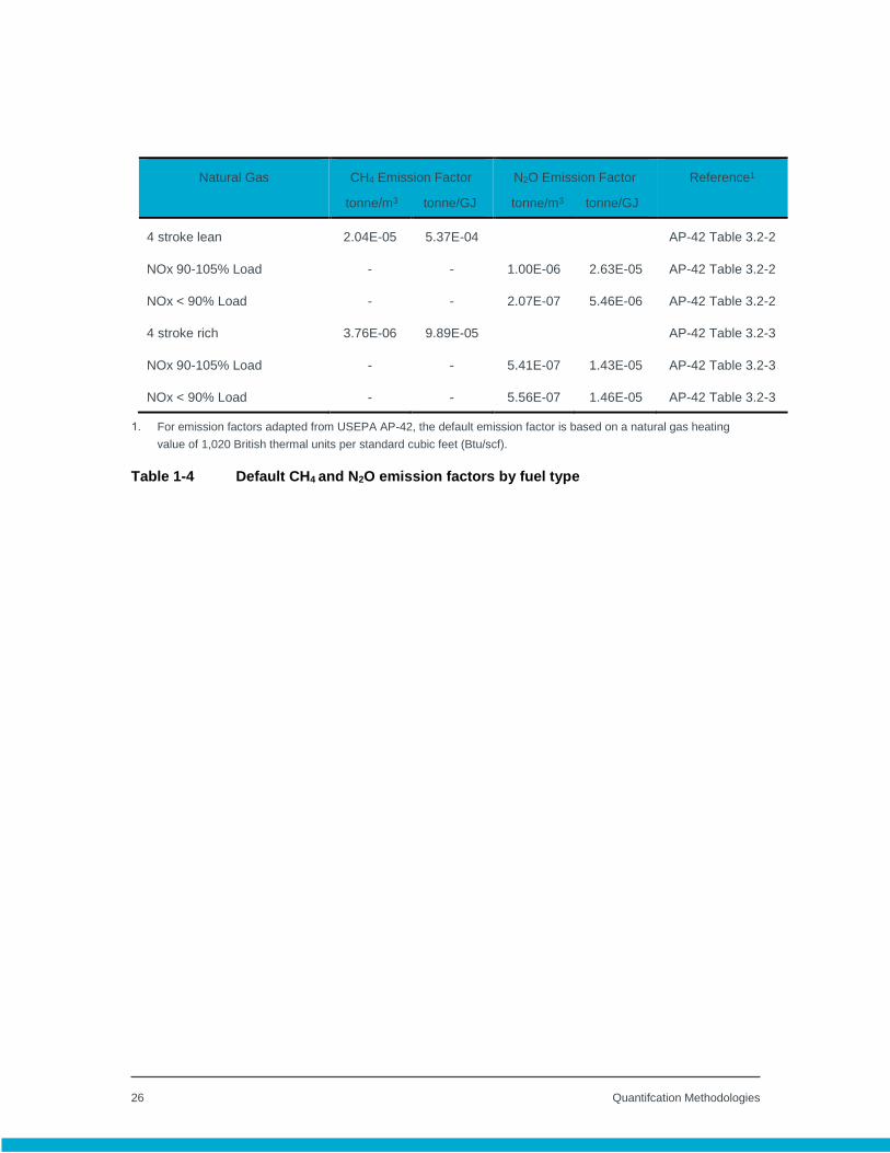
26 Quantifcation Methodologies
Natural Gas CH4 Emission Factor
tonne/m3 tonne/GJ
N2O Emission Factor
tonne/m3 tonne/GJ
Reference1
4 stroke lean 2.04E-05 5.37E-04 AP-42 Table 3.2-2
NOx 90-105% Load - - 1.00E-06 2.63E-05 AP-42 Table 3.2-2
NOx < 90% Load - - 2.07E-07 5.46E-06 AP-42 Table 3.2-2
4 stroke rich 3.76E-06 9.89E-05 AP-42 Table 3.2-3
NOx 90-105% Load - - 5.41E-07 1.43E-05 AP-42 Table 3.2-3
NOx < 90% Load - - 5.56E-07 1.46E-05 AP-42 Table 3.2-3
For emission factors adapted from USEPA AP-42, the default emission factor is based on a natural gas heating
value of 1,020 British thermal units per standard cubic feet (Btu/scf).
Table 1-4 Default CH4 and N2O emission factors by fuel type

27 Quantifcation Methodologies
Liquid Fuels1 CH4 Emission Factor
tonne/kl tonne/GJ
N2O Emission Factor
tonne/kl tonne/GJ
Kerosene
Electric Utilities 6.0E-06 2.0E-07 3.1E-05 8.3E-07
Industrial 6.0E-06 2.0E-07 3.1E-05 8.3E-07
Producer
Consumption1
6.0E-06 1.6E-07 3.1E-05 8.2E-07
Forestry, Construction
and
Commercial/Institution
2.6E-05 7.0E-07 3.1E-05 8.3E-07
Light Fuel Oil
Electric Utilities1 1.8E-04 4.6E-06 3.1E-05 7.99E-07
Industrial 6.0E-06 2.0E-07 3.1E-05 8.0E-07
Producer
Consumption1
6.0E-06 1.6E-07 3.1E-05 7.99E-07
Forestry, Construction
and Commercial
/Institution
2.6E-05 6.7E-07 3.1E-05 8.0E-07
Liquid Fuels1 CH4 Emission Factor
tonne/kl tonne/GJ
N2O Emission Factor
tonne/kl tonne/GJ
Heavy Fuel Oil
Electric Utilities 3.4E-05 8.0E-07 6.4E-05 1.5E-06
Industrial 1.2E-04 2.8E-06 6.4E-05 1.5E-06
Producer
Consumption2
1.2E-04 2.8E-06 6.4E-05 1.506E-06
Forestry, Construction
and Commercial
/Institution
5.7E-05 1.30E-06 6.4E-05 1.5E-06
Solid Fuels1 CH4 Emission Factor N2O Emission Factor

28 Quantifcation Methodologies
tonne/m3 tonne/GJ tonne/m3 tonne/GJ
Petroleum Coke - Refinery
Use
1.2E-04 2.6E-06 2.8E-05 5.9E-07
Petroleum Coke - Upgrader
Use
1.2E-04 3.0E-06 2.4E-05 5.9E-07
Coal
Electric Utilities
Anthracite 2.0E-05 8.0E-07 3.0E-05 1.0E-06
Canadian Bituminous 2.0E-05 8.0E-07 3.0E-05 1.0E-06
Foreign Bituminous 2.0E-05 7.0E-07 3.0E-05 1.0E-06
Lignite 2.0E-05 1.0E-06 3.0E-05 2.0E-06
Sub-bituminous 2.0E-05 1.0E-06 3.0E-05 2.0E-06
Industry and Heat and
Steam Plants
Anthracite 3.0E-05 1.0E-06 2.0E-05 7.0E-07
Canadian Bituminous 3.0E-05 1.0E-06 2.0E-05 7.0E-07
Foreign Bituminous 3.0E-05 1.0E-06 2.0E-05 7.0E-07
Solid Fuels1 CH4 Emission Factor N2O Emission Factor
tonne/m3 tonne/GJ tonne/m3 tonne/GJ
Lignite 3.0E-05 2.0E-06 2.0E-05 1.0E-06
Sub-bituminous 3.0E-05 2.0E-06 2.0E-05 1.0E-06
Residential, Public
Administration
Anthracite 4.0E-03 1.0E-04 2.0E-05 7.0E-07
Canadian Bituminous 4.0E-03 1.0E-04 2.0E-05 7.0E-07
Foreign Bituminous 4.0E-03 1.0E-04 2.0E-05 7.0E-07
Lignite 4.0E-03 2.0E-04 2.0E-05 1.0E-06

29 Quantifcation Methodologies
Sub-bituminous 4.0E-03 2.0E-04 2.0E-05 1.0E-06
Coke 3.0E-05 1.0E-06 2.0E-05 7.0E-07
Biomass Fuels1 CH4 Emission Factor N2O Emission Factor
tonne/tonne tonne/GJ tonne/tonne tonne/GJ
Wood Waste 9.0E-05 5.0E-06 6.0E-05 3.0E-06
Spent Pulping Liquor 2.0E-05 1.0E-06 2.0E-05 3.0E-06
Peat2 NA 1.0E-06 NA 1.5E-06
Gaseous Fuels1 CH4 Emission Factor
tonne/m3 tonne/GJ
N2O Emission Factor
tonne/m3 tonne/GJ
Coke Oven Gas 4.0E-08 2.0E-06 4.0E-08 2.0E-06
Still Gas3,4 3.1E-08 9.1E-07 2.0E-08 6.0E-07
Unless specified otherwise, emission factors are adapted from ECCC Canada's Greenhouse Gas Quantification
Requirements (Reference [3] in Appendix A).
WCI Table 20-2 or 20-7.
Adapted from IPCC (2006) and CIEEDAC (2014).
SGA (2000).
30 Quantifcation Methodologies
4.0 Quantification of Venting Emissions Venting emissions are from intentional or controlled releases to the atmosphere of a waste gas or
liquid stream that contains greenhouse gases (GHGs). Venting emissions are releases by design
or operational practice. Routine venting occurs either continuously or intermittently as part of
normal operations. Non-routine venting results in intermittent and infrequent emissions and can
be planned or unplanned under abnormal operation.
Methane (CH4) is the predominant specified gas contained in venting emissions but carbon
dioxide (CO2) can also be present in some venting emissions. Nitrous oxide (N2O) is not typically
vented unless a vented process stream contains this substance.
Venting emissions normally exist as part of upstream oil and gas (UOG) production, processing,
petroleum refining, oil sands and coal mining and upgrading industries in any facility that uses
natural gas (which typically is greater than 90 mol% methane) or process materials containing
CH4 or CO2. In Alberta, venting occurs predominantly in the UOG facilities. Venting emissions
also occur in chemical, coal mining, petrochemical, pipelines and fertilizer industries.
Venting emissions can be collected through vent gas capture systems, and then directed to
emissions control systems. The following emissions controls are generally used by industry:
Gas Conservation – where gas is captured and sold, used as fuel, injected into reservoirs for
pressure maintenance or other beneficial purpose.
Flare Systems – where gas is captured and combusted by thermal oxidization in a flare or
incinerator.
Scrubber Systems – where gas is captured and specific substances of concern (e.g. H2S) are
removed via adsorption or catalytic technologies.
If the vent gases are captured and directed to a fuel system or directed to a stationary fuel
combustion unit and/or flare stack, the emissions from these gases should be calculated under
stationary fuel combustion or flaring source categories. Destruction efficiencies of flaring are
considered under the flaring source categories, and are not to be reflected in the venting CF.
This chapter provides quantification methodologies for venting emissions from potential venting
sources in UOG, petroleum refining, petrochemical, fertilizer industries and other industries in
Alberta, which may have similar venting sources. Carbon dioxide emissions from industrial
process should be quantified according to the methodologies prescribed in the Chapter 8 for
31 Quantifcation Methodologies
industrial process (IP) emissions. Venting emissions due to biological reactions from waste
management or wastewater treatment facilities are classified as waste and wastewater
emissions. The methodologies for these emissions are prescribed in Chapter 6 for waste and
digestion emissions and Chapter 7 for wastewater emissions.
In this chapter, there may be one or more methodologies prescribed for a process that are not
tiered and therefore, are considered to be acceptable for use by a facility under any tier
classification. As well, facilities are permitted to use a higher tiered method to quantify the
facility’s emissions where appropriate. In addition, the chapter distinguishes venting emission
sources into routine and non-routine for emission quantifications purpose. However, CCIR and
SGRR do not require to report routine and non-routine venting emissions separately. Facilities
should aggregate total venting emissions for reporting.
For all sources discussed in this chapter, CO2 that is entrained in produced oil and gas are
considered to be formation CO2. Methodologies in this chapter are given for CH4 and CO2, but
CO2 will be reported as formation CO2 if it meets the definition of formation CO2. Imported CO2
and CO2 from IP are not considered to be formation CO2. For facilities reporting under CCIR,
formation CO2 emissions must be reported in a separate category; while facilities reporting under
SGRR must report venting and formation CO2 emissions under the venting category.
4.1 General Calculation
4.1.1 Control Factor (CF)
(1) Introduction
When a vent gas capture system is installed, venting emissions may still occur if the capture
equipment is not operating or functioning properly due to maintenance or periodic, planned, or
unplanned shutdowns, or emissions are not fully captured when the capture system is operating
due to capture system inefficiency. A control factor (CF) is introduced in this chapter to reflect the
efficiency of any venting capture system operation.
The CF should account for two factors that affect the final venting capture efficiency: collection
efficiency of the capture system and any downtime of the capture system. Therefore, CF should
be calculated by multiplying the capture system operation percentage of hours when the venting
sources are emitting in the report period by collection efficiency (percentage of GHGs that are
collected through the capture system), but should not reflect the destruction efficiency of a flare,
which is relevant to the flaring source category.

32 Quantifcation Methodologies
For instance, a control equipment is running 95% of the time when a venting source is emitting
and the capture efficiency is 98%, the CF = 95% (running time) * 98% (capture efficiency) =
93.1%. A facility may conduct an engineering assessment to determine the capture efficiency. In
cases where the system is fully enclosed, the facility may determine that the capture efficiency is
close to 100%.
(2) Equations
The CF for each emission source in the chapter is calculated using Equation 4-1a and should be
applied to all venting sources with a gas capture system.
𝑪𝑭 =𝒕 𝒐𝒑
𝒕 𝒕𝒐𝒕𝒂𝒍
× 𝒆𝒇𝒇𝒄𝒂𝒑𝒕𝒖𝒓𝒆 Equation 4-1a
Where:
CF = Control factor for venting emission source with a capture system in the
report period.
t op = Total uptime of capture system when the venting source is emitting
(hour) in the report period.
t total = Total hours of venting (hour) regardless of whether the capture system is
operating or not in the report period.
eff capture = Efficiency of capture system based on manufacturer data or engineering
design or assessment.
(3) Data requirements
Total operating hours of the capture system and total hours of the venting hours of the
venting source must be recorded.
Facilities are required to use manufacturer or design data and/or conduct an engineering
assessment to determine the efficiency of the capture system. This may be conducted once
for a capture system. If a new capture system is installed or there are changes to an existing
capture system, facilities are required to re-evaluate the capture efficiency.
Documents from manufacturer or engineering design and assessment must be available for
inspection or verification, if requested.

33 Quantifcation Methodologies
4.1.2 General Calculation-Periodic or Continuous Measurement
(1) Introduction
Vent gas streams may be required to be measured or tested through AER Directive 017 or
Directive 060 for UOG facilities or other applicable regulations for non-UOG facilities. Continuous
direct measurement or periodic testing of individual emission sources is encouraged where
possible and where these solutions would result in more accurate reporting of emissions than the
methods discussed. The following method is classified as a tier 4 methodology and applies to all
venting sources if a tier 4 methodology is not specifically prescribed for a venting source.
(2) Equations
Where periodic or continuous volumetric vent rate or volume is measured for vent streams,
calculate GHG emissions using Equation 4-1b.
𝑮𝑯𝑮 = ∑ 𝑽𝑹 𝒗 × 𝒕 × 𝑴𝑭𝑮𝑯𝑮
𝒏
𝒊=𝟏
× 𝝆 𝑮𝑯𝑮 × 𝟎. 𝟎𝟎𝟏 Equation 4-1b
Where:
GHG = CH4 or CO2 mass emissions from a venting source (tonnes) or vent gas
recovery system outlet venting to atmosphere in the report period.
i = Vent source or vent gas recovery system outlet.
N = Total number of vents or vent gas recovery system outlets venting to the
atmosphere in the report period. It is possible a number of vents are
connected to one outlet where the measured vent rate may represent the
total emissions from multiple vents.
VR v = Average volumetric vent rate at the vent or outlet of the recovery system
(Sm3/h). If the source or the gas recovery system is equipped with a
continuous meter, use the metered volume (Q, Sm3) in the report period to
replace VR*t. If a continuous vent meter is not available, periodic vent rate
measurement should measure the representative average vent rate for the
report period.
34 Quantifcation Methodologies
t = Venting time if the measurement is conducted at the vent source or
operating time of the recovery system if the measurement is conducted at
the outlet of the recovery system during the report period (hours).
MFGHG = Mole fraction of CO2 or CH4. Measured at the location where the vent rate
is measured; or if the vent rate measurement location has potential safety
issue for gas composition sampling, sample at a location where the gas
composition is the most representative of the vent gas composition.
GHG = Density of CO2 or CH4 at standard conditions (CO2 = 1.861 kg/sm3; CH4
= 0.6785 kg/sm3).
0.001 = Mass conversion factor (tonne/kg).
Where periodic or continuous mass vent rate or mass is measured for vent streams, calculate
GHG emissions using Equation 4-1c.
𝑮𝑯𝑮 = ∑ 𝑽𝑹 𝒎𝒂𝒔𝒔,𝒋 × 𝒕 × 𝑭 𝑮𝑯𝑮/𝒎𝒂𝒔𝒔,𝒋
𝒏
𝒊=𝟏
× 𝟎. 𝟎𝟎𝟏 Equation 4-1c
Where:
GHG = CH4 or CO2 mass emissions from a venting source (tonnes) in the report
period.
i = Vent source or vent gas recovery system outlet.
n = Total number of vents or vent gas recovery system outlets venting to the
atmosphere in the report period. It is possible a number of vents are
connected to one outlet where the measured vent rate may represent the
total emissions from multiple vents.
VR mass,j = Average vent rate at the vent or outlet of the recovery system (kg/h)
expressed in mass j. If the source or the gas recovery system is equipped
with a continuous meter, use the metered mass (kg) in the report period to
replace VRmass,j*t. If a continuous vent meter is not available, periodic vent
rate measurement should measure the representative average vent rate for
the report period.

35 Quantifcation Methodologies
j = Type of compound that is metered, such as total hydrocarbons (THCs),
total volatile organic compounds (VOCs), etc.
t = Venting time if the measurement is conducted at the vent source or
operating time of the recovery system if the measurement is conducted at
the outlet of the recovery system during the report period (hours).
F GHG/mass,j = Mass fraction of CO2 or CH4 to the mass j measured by the meter.
Measured at the location where the vent rate is measured.
0.001 = Mass conversion factor (tonne/kg).
(3) Data requirements
Periodic vent rate measurement at the outlet of the vent source or at the outlet of the vapor
recovery system if appropriate should be conducted under normal process operation. If the
measurement frequency is not prescribed for a particular source (as outlined throughout this
chapter), quarterly measurements are required at minimum for a facility operating
continuously in a year. If the facility does not operate for an entire quarter, the facility is not
required to sample in that quarter.
Facilities should follow meter installation, calibrations, vent rate measurement and vapor
composition sampling frequencies required by AER Directives. Non-UOG facilities may use
other applicable regulatory requirements or industry best practices for these parameters.
Volume measurements must be adjusted to standard conditions as defined in Appendix C.
If a continuous gas analyzer is installed on the outlet gas stream, then the continuous gas
analyzer results must be used.
Facilities may use the fuel gas composition if it is considered to be representative of the
vented gas.
Facilities are required to follow gas sampling frequencies prescribed in Table 17.3 of Chapter
17.
Gas compositions must be measured using:
o An applicable analytical method prescribed by AER Directives for UOG facilities;
o An analytical method prescribed in Section 17.2.3 of Chapter 17.
36 Quantifcation Methodologies
4.2 Routine Venting–Produced Gas at UOG Facilities
4.2.1 Introduction
Natural gas produced in conjunction with crude oil or bitumen is referred to as produced gas.
Produced gas may be gas dissolved in the oil that ‘flashes’ out upon depressurization or may be
a free ‘gas cap’ that was above the oil in the reservoir. Flashing losses are the dominant
contributor to produced gas volumes and occur at oil production sites where unstable
hydrocarbon liquids (i.e. products that have a vapor pressure greater than the local barometric
pressure) are produced into lower pressure vessels (separator) or atmospheric storage tanks.
These types of emissions occur at UOG facilities.
Ideally, produced gas is conserved with gathering pipelines or utilized as combustion fuel.
However, stranded gas is often flared or vented. If the produced gas is conserved and used as
fuel at the site, the emissions should be calculated according to Chapter 1 Stationary Fuel
Combustion. If the produced gas is captured and flared, the emissions should be calculated
according to Chapter 2 Flaring.
4.2.2 Tier 1-Rule-of-Thumb Method
(1) Introduction
The produced gas volume relates to the hydrocarbon liquid production volume and the Gas in
Solution (GIS). The emissions calculated by the following method are based on the rule of thumb
GIS estimation in AER Directive 017. This approach is applicable for light-medium oil production.
The CO2 emissions calculated using the equations below are considered to be formation CO2.
(2) Equations
Calculate GHG emissions using Equation 4-2a.
𝑮𝑯𝑮 = 𝑸 𝒐𝒊𝒍 × 𝑮𝑰𝑺 × 𝝆 𝑮𝑯𝑮 × 𝑴𝑭 𝑮𝑯𝑮/𝑮𝒂𝒔 × 𝟎. 𝟎𝟎𝟏 × (𝟏 − 𝑪𝑭) Equation 4-2a
Where:
GHG = CH4 or CO2 mass emissions from produced gas venting (tonnes) in the
report period.
Q oil = Total volume of oil produced for the report period, (m3 oil).

37 Quantifcation Methodologies
GIS = A rule-of-thumb value calculated using Equation 4-2b, which represents
the amount of gas dissolved in a volume of hydrocarbon liquid produced
(of all API gravities), and is correlated to the amount of pressure drop
between the reservoir and the current vessel.
MF GHG/Gas = Mole fraction of CO2 or CH4 in vented gas.
CF = Venting control factor (dimensionless). This accounts for collection
efficiency of the capture system as well as any downtime of the capture
system, calculated using Equation 4-1a. CF is zero if no capture system
is installed.
GHG = Density of CO2 or CH4 at standard conditions (CO2 = 1.861 kg/sm3; CH4 =
0.6785 kg/sm3).
0.001 = Mass conversion factor (tonne/kg).
𝑮𝑰𝑺 = 𝟎. 𝟎𝟐𝟓𝟕 × ∆𝑷 Equation 4-2b
Where:
ΔP = Pressure drop between the well reservoir and the vessel (kPa) at well
site.
0.0257 = GIS coefficient (sm3 gas/sm3 oil/kPa of pressure drop).
(3) Data requirements
For this method, facilities are required to follow AER Directive 017 for conventional light-
medium oil production measurement and reporting requirements.
The control technology and operating time in the report period must be documented.
38 Quantifcation Methodologies
4.2.3 Tiers 2, 3, and 4-AER Directive 017 Measurements and
Estimation Methods
(1) Introduction
Produced gas from a well must be determined based on the requirements of AER Directive 017.
This may include continuous direct metering or periodic measurement. The GIS should be
representative of vented gas volume and production volume during normal process operations.
Facilities are expected to select the most representative methodology from Directive 017 to
quantify vented emissions.
In cases where all produced gas is vented, the vent gas volume is equal to the produced gas
volume.
(2) Equations
Equation 4-2a is used with a measured GIS value, which should be determined according to AER
Directive 017.
(3) Data requirements
The GIS must be determined by applicable tests, procedures and requirements for the
equipment outlined in AER Directive 017 for the specific process scenario (i.e. single well
battery, multiwell oil proration battery, etc.)
GIS measurement method and frequency must follow Section 12.2.2 and Table 12.1 in
Directive 017 for crude bitumen facilities.
Oil production must be the oil-produced volume in the corresponding duration when the gas
volume is tested.
Facilities are required to follow AER Directive 017 to calculate production quantities.
An extended hydrocarbon analysis of the flash gas from the GIS sample may be conducted if
the gas composition is changing.
39 Quantifcation Methodologies
4.3 Routine Venting-Continuous Gas Analyzer Purge
4.3.1 Tiers 1, 2 and 3-Default Vent Rate
(1) Introduction
An online gas analyzer normally draws a continuous stream of sample. It uses some fraction of
this stream and then vents both the unused and spent portions to the atmosphere. Depending on
the type of analyzer, the used portion of sample may be released unchanged or as a product of
combustion. The amount of emissions depends on the sampling rate and the characteristics of
the analyzer. The emissions quantification method provided is applicable to tiers 1, 2, and 3.
(2) Equations
Calculate GHG emissions using Equation 4-3.
𝑮𝑯𝑮 = ∑ ∑ 𝑸 𝒗 × 𝑴𝑭 𝑮𝑯𝑮 × 𝝆 𝑮𝑯𝑮 × 𝟎. 𝟎𝟎𝟏
𝒏
𝒊
𝒎
𝒋
Equation 4-3
Where:
GHG = CH4 or CO2 mass emissions from gas analyzer (tonnes) in the report
period.
i = Analyzer identifier.
j = Month identifier.
n = Total number of analyzers used in a month.
m = Total months in the report period.
Q v = Vented gas volume per analyzer per month (sm3/analyzer/month) at the
standard condition during the report period.
MF GHG = Mole fraction of CO2 or CH4 in the vented gas. Using the average gas
analysis per analyzer for the report period.

40 Quantifcation Methodologies
GHG = Density of CO2 or CH4 at standard conditions (CO2 = 1.861 kg/sm3; CH4 =
0.6785 kg/sm3).
0.001 = Mass conversion factor (tonne/kg).
(3) Data requirements
The vent rate from the analyzer may be based on manufacturer data or an engineering
estimate. If an average vent rate for upstream oil and gas installations is not available, 69.8
m3 of natural gas/month/analyzer could be used for each analyzer on a natural gas
transmission pipeline.
The facility is required to apply the gas analysis measured by the gas analyzer itself.
If multiple analysis is done in a month, use an average of the gas compositions.
Volume measurements must be adjusted to standard conditions as defined in Appendix C.
4.4 Routine Venting-Solid Desiccant Dehydrators
4.4.1 Tiers 1, 2 and 3-Physical Volume Depression
(1) Introduction
Desiccant dehydrators are filled with solid desiccants, which absorb water from a gas stream.
Solid desiccants employed in the upstream oil & gas industry include silica gel, activated alumina
and molecular sieves. Desiccant dehydrators typically feature at least two vessels that operate in
a cyclic manner alternating between drying and regeneration. There are various ways to
regenerate a dryer, including recycling a portion of the product stream, or some other gas stream.
In some cases, a heated gas stream passes through the desiccant to desorb water and is
typically recycled back to the wet gas flow so zero venting occurs during normal operation.
However, gas can be vented each time the vessel is depressurized for desiccant refilling. The
following equation reflects the emissions from the desiccant dehydrator depressurization
emissions.
(2) Equations
For each desiccant dehydrator venting event, calculate CH4 or CO2 emissions separately and
then add the emissions in the report period based on total events using the following equation.
The CO2 emissions calculated using the equations below are considered to be formation CO2.
41 Quantifcation Methodologies
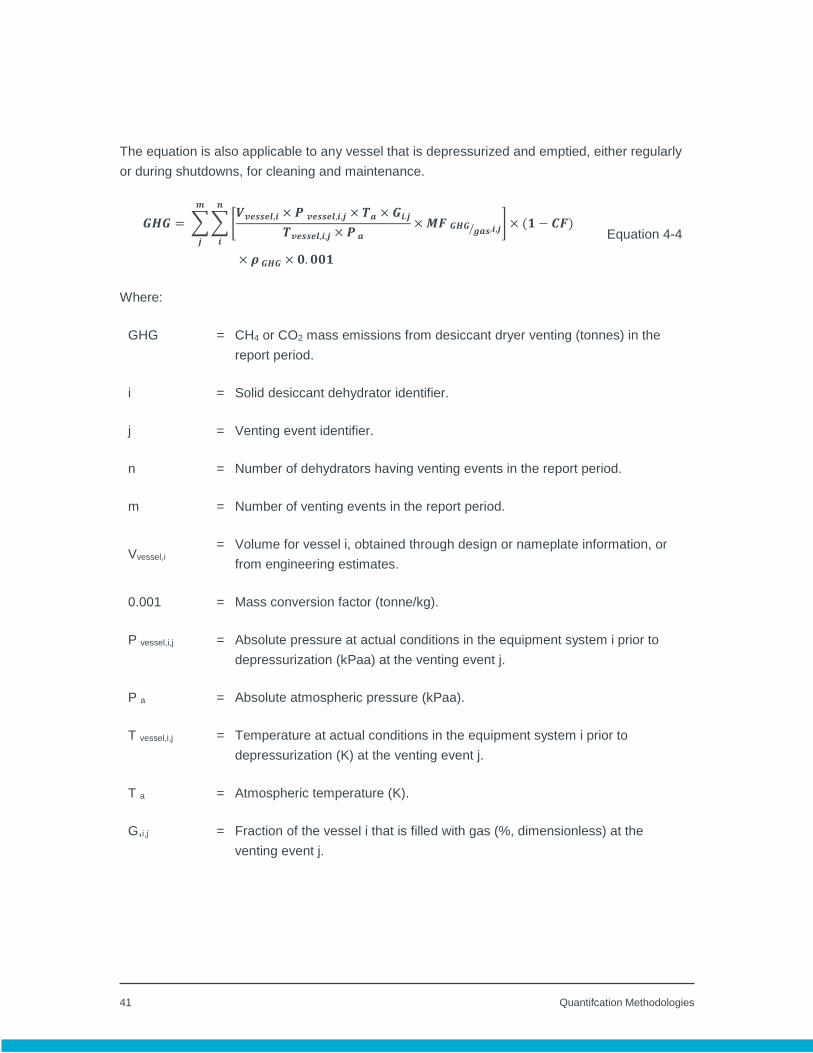
The equation is also applicable to any vessel that is depressurized and emptied, either regularly
or during shutdowns, for cleaning and maintenance.
𝑮𝑯𝑮 = ∑ ∑ [𝑽𝒗𝒆𝒔𝒔𝒆𝒍,𝒊 × 𝑷 𝒗𝒆𝒔𝒔𝒆𝒍,𝒊,𝒋 × 𝑻𝒂 × 𝑮𝒊.𝒋
𝑻𝒗𝒆𝒔𝒔𝒆𝒍,𝒊,𝒋 × 𝑷 𝒂
× 𝑴𝑭 𝑮𝑯𝑮𝒈𝒂𝒔⁄ ,𝒊,𝒋]
𝒏
𝒊
𝒎
𝒋
× (𝟏 − 𝑪𝑭)
× 𝝆 𝑮𝑯𝑮 × 𝟎. 𝟎𝟎𝟏
Equation 4-4
Where:
GHG = CH4 or CO2 mass emissions from desiccant dryer venting (tonnes) in the
report period.
i = Solid desiccant dehydrator identifier.
j = Venting event identifier.
n = Number of dehydrators having venting events in the report period.
m = Number of venting events in the report period.
Vvessel,i = Volume for vessel i, obtained through design or nameplate information, or
from engineering estimates.
0.001 = Mass conversion factor (tonne/kg).
P vessel,i,j = Absolute pressure at actual conditions in the equipment system i prior to
depressurization (kPaa) at the venting event j.
P a = Absolute atmospheric pressure (kPaa).
T vessel,i,j = Temperature at actual conditions in the equipment system i prior to
depressurization (K) at the venting event j.
T a = Atmospheric temperature (K).
G,i,j = Fraction of the vessel i that is filled with gas (%, dimensionless) at the
venting event j.
42 Quantifcation Methodologies
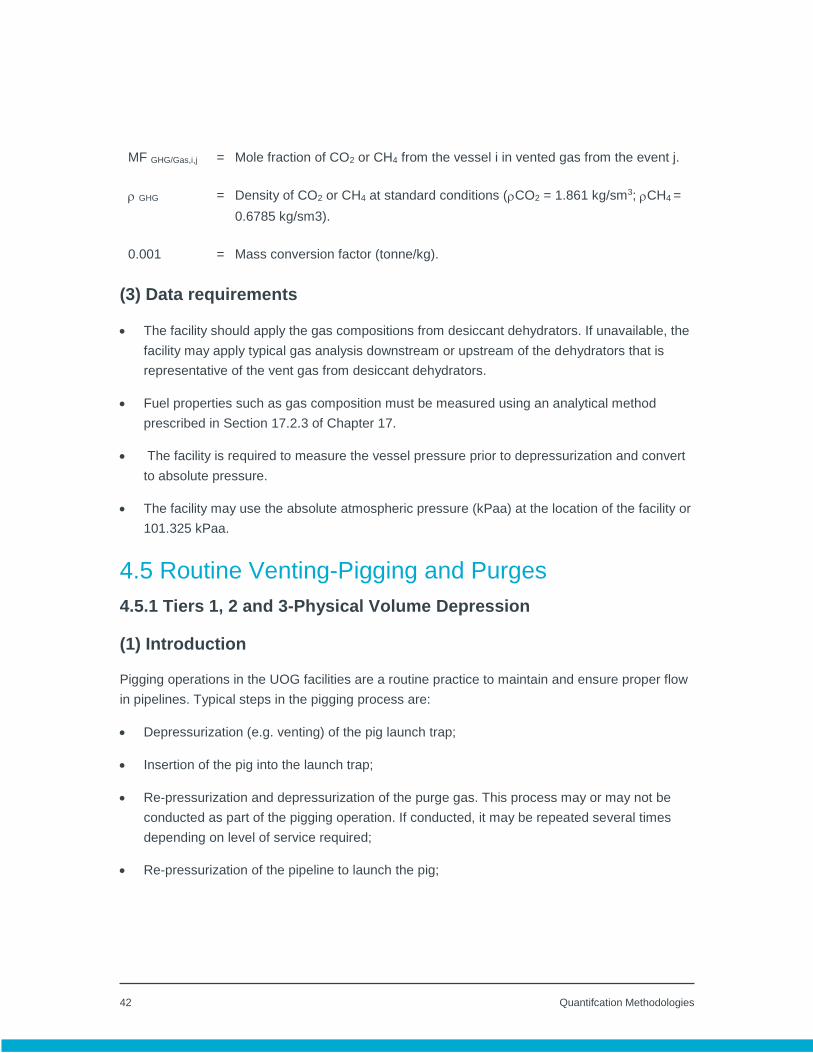
MF GHG/Gas,i,j = Mole fraction of CO2 or CH4 from the vessel i in vented gas from the event j.
GHG = Density of CO2 or CH4 at standard conditions (CO2 = 1.861 kg/sm3; CH4 =
0.6785 kg/sm3).
0.001 = Mass conversion factor (tonne/kg).
(3) Data requirements
The facility should apply the gas compositions from desiccant dehydrators. If unavailable, the
facility may apply typical gas analysis downstream or upstream of the dehydrators that is
representative of the vent gas from desiccant dehydrators.
Fuel properties such as gas composition must be measured using an analytical method
prescribed in Section 17.2.3 of Chapter 17.
The facility is required to measure the vessel pressure prior to depressurization and convert
to absolute pressure.
The facility may use the absolute atmospheric pressure (kPaa) at the location of the facility or
101.325 kPaa.
4.5 Routine Venting-Pigging and Purges
4.5.1 Tiers 1, 2 and 3-Physical Volume Depression
(1) Introduction
Pigging operations in the UOG facilities are a routine practice to maintain and ensure proper flow
in pipelines. Typical steps in the pigging process are:
Depressurization (e.g. venting) of the pig launch trap;
Insertion of the pig into the launch trap;
Re-pressurization and depressurization of the purge gas. This process may or may not be
conducted as part of the pigging operation. If conducted, it may be repeated several times
depending on level of service required;
Re-pressurization of the pipeline to launch the pig;
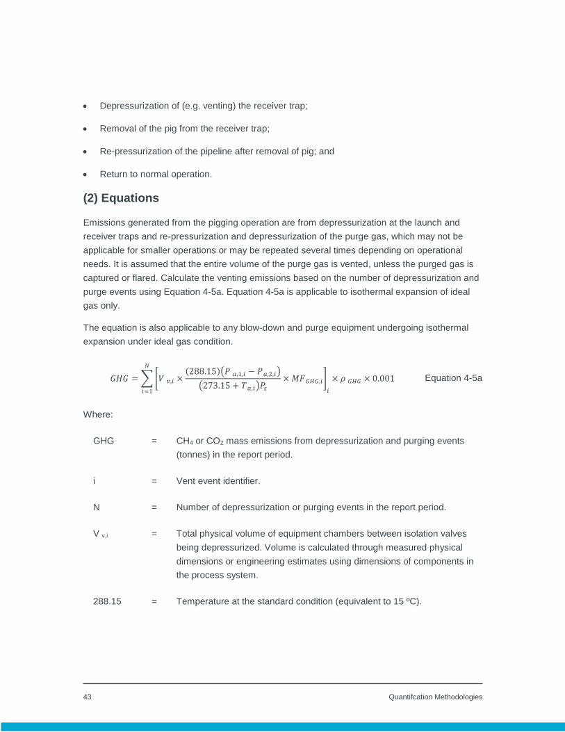
43 Quantifcation Methodologies
Depressurization of (e.g. venting) the receiver trap;
Removal of the pig from the receiver trap;
Re-pressurization of the pipeline after removal of pig; and
Return to normal operation.
(2) Equations
Emissions generated from the pigging operation are from depressurization at the launch and
receiver traps and re-pressurization and depressurization of the purge gas, which may not be
applicable for smaller operations or may be repeated several times depending on operational
needs. It is assumed that the entire volume of the purge gas is vented, unless the purged gas is
captured or flared. Calculate the venting emissions based on the number of depressurization and
purge events using Equation 4-5a. Equation 4-5a is applicable to isothermal expansion of ideal
gas only.
The equation is also applicable to any blow-down and purge equipment undergoing isothermal
expansion under ideal gas condition.
𝐺𝐻𝐺 = ∑ [𝑉 𝑣,𝑖 ×(288.15)(𝑃 𝑎,1,𝑖 − 𝑃 𝑎,2,𝑖)
(273.15 + 𝑇 𝑎,𝑖)𝑃𝑠
× 𝑀𝐹 𝐺𝐻𝐺,𝑖]𝑖
𝑁
𝑖=1
× 𝜌 𝐺𝐻𝐺 × 0.001 Equation 4-5a
Where:
GHG = CH4 or CO2 mass emissions from depressurization and purging events
(tonnes) in the report period.
i = Vent event identifier.
N = Number of depressurization or purging events in the report period.
V v,i = Total physical volume of equipment chambers between isolation valves
being depressurized. Volume is calculated through measured physical
dimensions or engineering estimates using dimensions of components in
the process system.
288.15 = Temperature at the standard condition (equivalent to 15 ºC).

44 Quantifcation Methodologies
T a,i = Initial temperature of gas at actual conditions in the equipment system
prior to depressurization or purge (ºC).
P s = Absolute atmospheric pressure at standard conditions (101.325 kPa).
P a,1,i = Absolute pressure at actual conditions in the equipment system prior to
depressurization or purge (kPaa).
P a,2,i = Absolute pressure at actual conditions in the equipment system after
depressurization or purge (kpaa). This pressure may be assumed to be
the same as the absolute atmospheric pressure (Ps) if this measurement is
not taken .
MF GHG,i = Mole fraction of CO2 or CH4 in the vented gas at the depressurization or
purging event i.
GHG = Density of CO2 or CH4 at standard conditions (CO2 = 1.861 kg/sm3; CH4 =
0.6785 kg/sm3).
0.001 = Mass conversion factor (tonne/kg).
For non-ideal gas scenarios, Equation 4-5b may be used. Equation 4-5b assumes an initial period
when the equipment is isolated and depressurized with no flow into the equipment, followed by a
period of purge gas flow through the equipment where the entire volume of the purge gas is
vented to atmosphere. Equation 4-5b can also be used if the equipment is not purged with gas
prior to repressurization by setting the mPurge or tpurge term equal to zero. If the assumptions for
Equation 4-5b are not valid, engineering estimates may be used to quantify greenhouse gas
emissions from pigging and purge operations.
𝑮𝑯𝑮 = ∑[(𝑽 𝒗 × (𝝆 𝒂,𝟏 − 𝝆 𝒂,𝟐) × 𝑭 𝑮𝑯𝑮/𝒗𝒂𝒑𝒐𝒓)
𝒏
𝒊=𝟎
+ (��𝑷𝒖𝒓𝒈𝒆 × 𝒕𝒑𝒖𝒓𝒈𝒆 × 𝑭 𝑮𝑯𝑮/𝑷𝒖𝒓𝒈𝒆)] × 𝟎. 𝟎𝟎𝟏
Equation 4-5b
Where:
GHG = CH4 or CO2 mass emissions from pigging and purges (tonnes) in the
report period.

45 Quantifcation Methodologies
i = Vent event identifier.
n = Total number of events in the report period.
ρ a,1 = Density of gas in equipment chamber at actual conditions prior to
depressurization, as estimated using real gas properties or by suitable
equation of state, kg/m3.
ρ a,2 = Density of gas in pigging equipment chamber after depressurization, as
estimated using real gas properties or by suitable equation of state, kg/m3.
If the equipment is purged following depressurization, 𝝆 𝒂,𝟐 = 0.
V v = Total physical volume of pigging equipment between isolation valves being
depressurized. Volume is calculated through measured physical
dimensions or engineering estimates using dimensions of components
(m3).
mPurge = Mass flow rate of gas used to purge equipment (kg/s).
tpurge = Duration of equipment purge event(s).
F GHG/Vapor = Mass fraction of CH4 or CO2 components in vapor during depressurization.
F GHG/purge = Mass fraction of CH4 or CO2 components in purge during depressurization.
0.001 = Mass conversion factor (tonne/kg).
(3) Data requirements
Actual pressure and temperature before and after each depressurization and purging event
should be metered and documented.
When the purge gas contains greenhouse gas components, the duration and mass flow rate
of purge gas used for each purging event should be estimated and documented.
Facilities are required to use the gas composition in the period closest to when the pigging
operation occurred.
Gas properties such as gas composition must be measured using an analytical method
prescribed in Section 17.2.3 of Chapter 17.
46 Quantifcation Methodologies
4.6 Routine Venting-Atmospheric Liquid Storage Tank
4.6.1 Introduction
GHG emissions can occur from atmospheric pressure fixed-roof and floating-roof storage tanks
receiving hydrocarbon liquids. Floating roof tanks control vapor spaces by lowering and lifting the
tank roof to reduce the vapor accumulation on top of the storage liquid. These tanks are common
in various types of facilities that process or store hydrocarbons.
There are typically three types of activities that release emissions from storage tanks:
Evaporative losses from the storage of hydrocarbons are known as breathing (or standing)
losses and are caused by changes in daily temperature or barometric pressure.
Evaporative losses during tank filling and emptying operations are known as working losses
and are caused by the displacement of tank vapors during liquid level changes.
Flashing losses when pressurized hydrocarbon liquids are delivered from higher-pressure
separators to lower-pressure storage tanks.
The main areas where tank flashing losses occur are at:
Wellhead sites when produced liquids are sent to an atmospheric storage vessel from the last
pressurized vessel;
Tank batteries when produced liquids are sent to an atmospheric storage vessel from the last
pressurized vessel;
Compressors stations when produced liquids are sent to an atmospheric storage vessel from
the last pressurized vessel;
Gas plants when produced liquids are sent to an atmospheric storage vessel from the last
pressurized vessel; and/or
When the liquids in the gas lines are “pigged” (physically purged of condensate) and then
sent to an atmospheric storage vessel.
The tank venting is from the vapor space at the top of the tank, which includes mostly volatile
hydrocarbons.
These methodologies are not intended for the following types of equipment:

47 Quantifcation Methodologies
Units permanently attached to conveyances such as trucks, trailers, rail cars, barges, or
ships;
Pressure vessels designed to operate in excess of 204.9 kilopascals and without emissions
to the atmosphere;
Bottoms receivers or sumps;
Vessels storing wastewater;
Reactor vessels associated with a manufacturing process unit.
Emissions from these types of equipment are addressed in other chapters of this document.
Quantification methodologies are prescribed in this section to cover petroleum liquids, pure
volatile organic liquids, and other types of chemical mixtures. However, not all methods are
applicable for all types of liquids. The reporter is required to select the most appropriate method
based on the type of tank system and tank contents.
The total venting emissions from tanks should be the sum of all three types of emissions including
flashing, breathing, and working losses for the reporting period. Table 4-1 assigns the
methodologies to be used based on the applicable tier classifications. A reporter may choose to
calculate tank emissions separately for flashing, breathing, and working losses and then
aggregate these emissions (Approach 1) or calculate the total emissions (Approach 2).
Figure 4-1 Tier Classification and Methodology Mapping
Tank Total
Emissions
Category of
Tank Emission
Tier Classification
Tier 1 Tier 2 Tier 3 Tier 4
Approach 1
Tank breathing
and working
losses Use engineering estimates for
facilities other than refineries.
Method 2
Method 7
Tank flashing
losses
Method 3
or 4 Method 5
Approach 2 Tank total
emissions
Method 1 for refineries. Use
engineering estimates for
facilities other than refineries.
Method 6
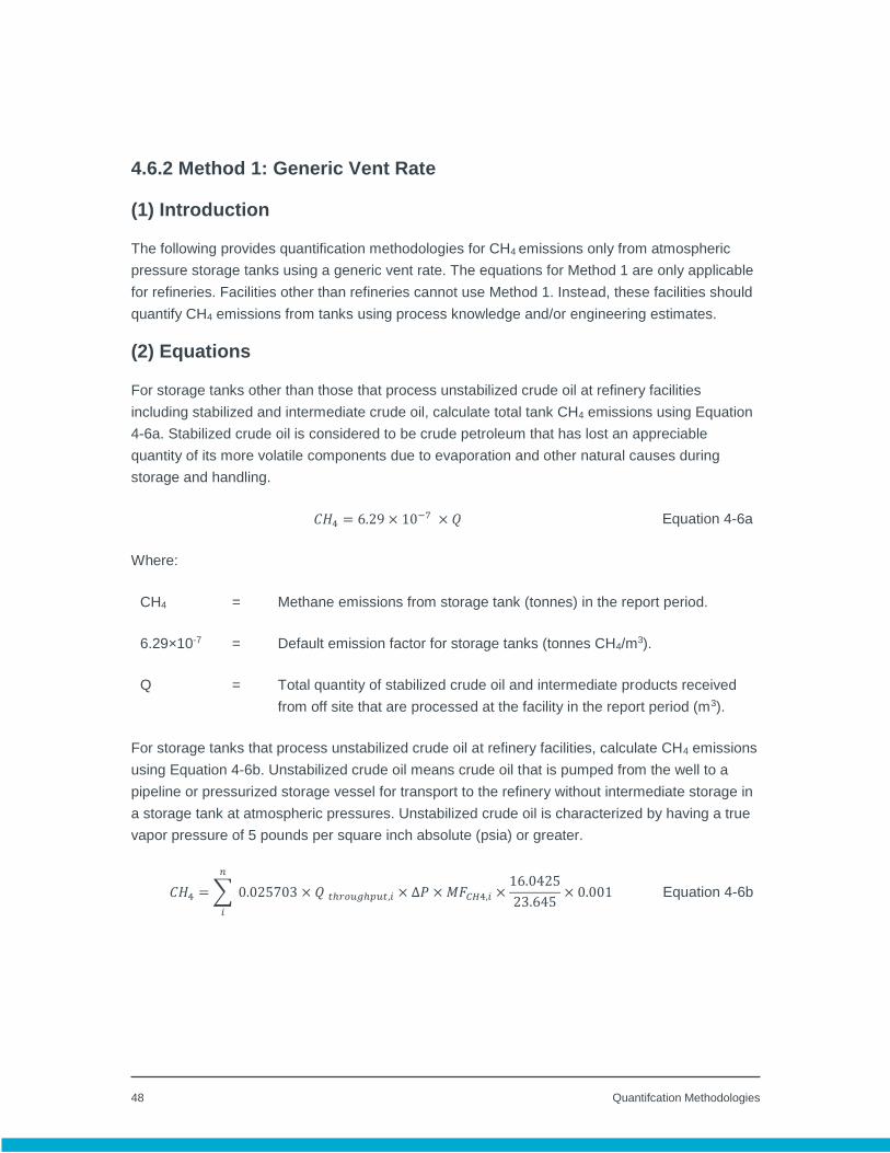
48 Quantifcation Methodologies
4.6.2 Method 1: Generic Vent Rate
(1) Introduction
The following provides quantification methodologies for CH4 emissions only from atmospheric
pressure storage tanks using a generic vent rate. The equations for Method 1 are only applicable
for refineries. Facilities other than refineries cannot use Method 1. Instead, these facilities should
quantify CH4 emissions from tanks using process knowledge and/or engineering estimates.
(2) Equations
For storage tanks other than those that process unstabilized crude oil at refinery facilities
including stabilized and intermediate crude oil, calculate total tank CH4 emissions using Equation
4-6a. Stabilized crude oil is considered to be crude petroleum that has lost an appreciable
quantity of its more volatile components due to evaporation and other natural causes during
storage and handling.
𝐶𝐻4 = 6.29 × 10⁻⁷ × 𝑄 Equation 4-6a
Where:
CH4 = Methane emissions from storage tank (tonnes) in the report period.
6.29×10-7 = Default emission factor for storage tanks (tonnes CH4/m3).
Q = Total quantity of stabilized crude oil and intermediate products received
from off site that are processed at the facility in the report period (m3).
For storage tanks that process unstabilized crude oil at refinery facilities, calculate CH4 emissions
using Equation 4-6b. Unstabilized crude oil means crude oil that is pumped from the well to a
pipeline or pressurized storage vessel for transport to the refinery without intermediate storage in
a storage tank at atmospheric pressures. Unstabilized crude oil is characterized by having a true
vapor pressure of 5 pounds per square inch absolute (psia) or greater.
𝐶𝐻4 = ∑ 0.025703 × 𝑄 𝑡ℎ𝑟𝑜𝑢𝑔ℎ𝑝𝑢𝑡,𝑖 × ∆𝑃 × 𝑀𝐹𝐶𝐻4,𝑖
𝑛
𝑖
×16.0425
23.645× 0.001 Equation 4-6b

49 Quantifcation Methodologies
Where:
CH4 = Methane emissions from storage tank (tonnes) in the report period.
i = Tank identifier.
n = Number of tanks in the report period.
0.025703 = Correlation equation factor (m3 gas per m3 oil per kpaa).
Q throughput,i = Total throughputs of un-stabilized crude oil in the tank i in the report
period (m3).
∆𝑃 = Pressure difference from the previous storage pressure to atmospheric
pressure (kpaa).
MF CH4,i = Mole fraction of CH4 in vent gas from the unstabilized crude oil storage
tank from facility measurements (kg-mole CH4/kg-mole gas); use 0.27 as
a default for refineries if measured data are not available.
16 = Molecular weight of methane (kg/kmol).
22.4 = Molar volume conversion factor (m3/kmol).
0.001 = Conversion factor (tonne/kg).
(3) Data requirements
Actual pressure at the upstream storage should be metered and documented.
Facilities are required to use the metered product throughputs if a meter is installed for each
storage tank; if metering is not available, facilities may use the throughputs used for
accounting purposes.
Facilities may use the atmospheric pressure at the location of the facility or 101.325
kilopascals for Equation 4-6b.
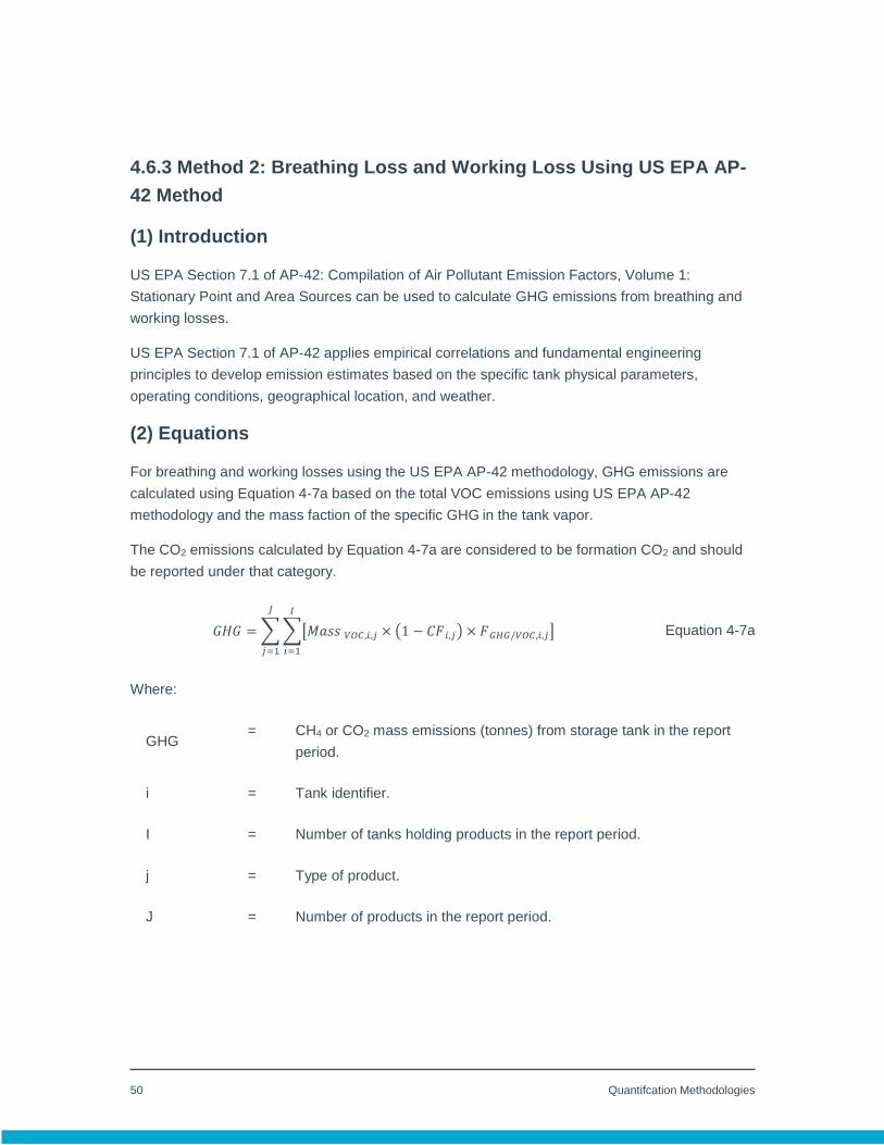
50 Quantifcation Methodologies
4.6.3 Method 2: Breathing Loss and Working Loss Using US EPA AP-
42 Method
(1) Introduction
US EPA Section 7.1 of AP-42: Compilation of Air Pollutant Emission Factors, Volume 1:
Stationary Point and Area Sources can be used to calculate GHG emissions from breathing and
working losses.
US EPA Section 7.1 of AP-42 applies empirical correlations and fundamental engineering
principles to develop emission estimates based on the specific tank physical parameters,
operating conditions, geographical location, and weather.
(2) Equations
For breathing and working losses using the US EPA AP-42 methodology, GHG emissions are
calculated using Equation 4-7a based on the total VOC emissions using US EPA AP-42
methodology and the mass faction of the specific GHG in the tank vapor.
The CO2 emissions calculated by Equation 4-7a are considered to be formation CO2 and should
be reported under that category.
𝐺𝐻𝐺 = ∑ ∑[𝑀𝑎𝑠𝑠 𝑉𝑂𝐶,𝑖,𝑗 × (1 − 𝐶𝐹 𝑖,𝑗) × 𝐹 𝐺𝐻𝐺/𝑉𝑂𝐶,𝑖,𝑗]
𝐼
𝑖=1
𝐽
𝑗=1
Equation 4-7a
Where:
GHG = CH4 or CO2 mass emissions (tonnes) from storage tank in the report
period.
i = Tank identifier.
I = Number of tanks holding products in the report period.
j = Type of product.
J = Number of products in the report period.

51 Quantifcation Methodologies
Mass VOC,i,j = Total VOC mass emissions calculated using US EPA AP-42
methodology from product j throughputs in tank i in the report period.
CF = Control factor (dimensionless fraction).
F GHG/VOC,i,j = Mass fraction of CH4 or CO2 in the vented VOCs for product j in tank i.
(3) Data requirements
For the mass fraction, the facility may use a measured value, engineering estimate, or default
compositions presented in Tables 3-2a to 3-2e in Chapter 3 Fugitives. Tables 3-2a to 3-2e
from Chapter 3 have been temporarily provided in this chapter for reference.
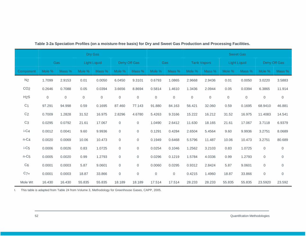
52 Quantifcation Methodologies
Table 3-2a Speciation Profiles (on a moisture-free basis) for Dry and Sweet Gas Production and Processing Facilities.
Dry Gas Sweet Gas
Gas Light Liquid Dehy Off Gas Gas Tank Vapors Light Liquid Dehy Off Gas
Component Mole % Mass % Mole % Mass % Mole % Mass % Mole % Mass % Mole % Mass % Mole % Mass % Mole % Mass %
N2 1.7099 2.9153 0.01 0.0050 6.0450 9.3101 0.6793 1.0865 2.9668 2.9436 0.01 0.0050 3.0220 3.5883
CO2 0.2646 0.7088 0.05 0.0394 3.6656 8.8694 0.5814 1.4610 1.3436 2.0944 0.05 0.0394 6.3865 11.914
H2S 0 0 0 0 0 0 0 0 0 0 0 0 0 0
C1 97.291 94.998 0.59 0.1695 87.460 77.143 91.880 84.163 56.421 32.060 0.59 0.1695 68.9410 46.881
C2 0.7009 1.2828 31.52 16.975 2.8296 4.6780 5.4263 9.3166 15.222 16.212 31.52 16.975 11.4083 14.541
C3 0.0295 0.0792 21.61 17.067 0 0 1.0490 2.6412 11.630 18.165 21.61 17.067 3.7118 6.9379
i-C4 0.0012 0.0041 9.60 9.9936 0 0 0.1291 0.4284 2.6504 5.4564 9.60 9.9936 3.2751 8.0689
n-C4 0.0020 0.0069 10.06 10.473 0 0 0.1949 0.6468 5.5796 11.487 10.06 10.473 3.2751 80.689
i-C5 0.0006 0.0026 0.83 1.0725 0 0 0.0254 0.1046 1.2562 3.2103 0.83 1.0725 0 0
n-C5 0.0005 0.0020 0.99 1.2793 0 0 0.0296 0.1219 1.5784 4.0336 0.99 1.2793 0 0
C6 0.0001 0.0003 5.87 9.0601 0 0 0.0060 0.0295 0.9312 2.8424 5.87 9.0601 0 0
C7+ 0.0001 0.0003 18.87 33.866 0 0 0 0 0.4215 1.4960 18.87 33.866 0 0
Mole Wt 16.430 16.430 55.835 55.835 18.189 18.189 17.514 17.514 28.233 28.233 55.835 55.835 23.5920 23.592
This table is adapted from Table 24 from Volume 3, Methodology for Greenhouse Gases, CAPP, 2005.

53 Quantifcation Methodologies
Table 3-2b Speciation Profiles (on a moisture-free basis) for Sour Gas Production and Processing Facilities and for Natural Gas
Transmission Facilities.
Sour Gas Natural Gas
Gas Tank Vapors Light Liquid Gas
Component Mole % Mass % Mole % Mass % Mole % Mass % Mole % Mass %
N2 0.6552 1.0140 2.9668 2.9436 0.01 0.0050 0.7791 1.2500
CO2 0.5608 1.3635 1.3436 2.0944 0.05 0.0394 0.6160 1.5527
H2S 3.5460 6.6755 0.0000 0.0000 0.00 0.0000 0.0000 0.0000
C1 88.6210 78.5447 56.4205 32.0598 0.59 0.1695 92.5394 85.0226
C2 5.2339 8.6947 15.2219 16.2121 31.52 16.9753 4.5125 7.7709
C3 1.0118 2.4649 11.6300 18.1646 21.61 17.0671 1.0904 2.7538
i-C4 0.1245 0.3998 2.6504 5.4564 9.60 9.9936 0.1498 0.4985
n-C4 0.1880 0.6037 5.5796 11.4867 10.06 10.4725 0.2103 0.7000
i-C5 0.0245 0.0977 1.2562 3.2103 0.83 1.0725 0.0415 0.1716
n-C5 0.0286 0.1140 1.5784 4.0336 0.99 1.2793 0.0358 0.1478
C6 0.0058 0.0276 0.9312 2.8424 5.87 9.0601 0.0170 0.0839
C7+ 0.0000 0.0000 0.4215 1.4960 18.87 33.8656 0.0084 0.0482
Mole Wt 18.1011 18.1011 28.2333 28.2333 55.8345 55.8345 17.4613 17.4613
This table is adapted from Table 25 from Volume 3, Methodology for Greenhouse Gases, CAPP, 2005.
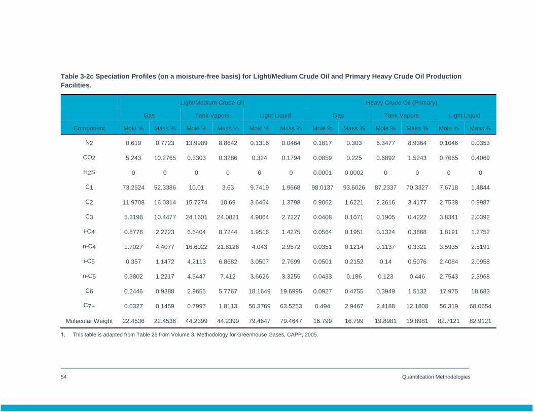
54 Quantifcation Methodologies
Table 3-2c Speciation Profiles (on a moisture-free basis) for Light/Medium Crude Oil and Primary Heavy Crude Oil Production
Facilities.
Light/Medium Crude Oil Heavy Crude Oil (Primary)
Gas Tank Vapors Light Liquid Gas Tank Vapors Light Liquid
Component Mole % Mass % Mole % Mass % Mole % Mass % Mole % Mass % Mole % Mass % Mole % Mass %
N2 0.619 0.7723 13.9989 8.8642 0.1316 0.0464 0.1817 0.303 6.3477 8.9364 0.1046 0.0353
CO2 5.243 10.2765 0.3303 0.3286 0.324 0.1794 0.0859 0.225 0.6892 1.5243 0.7665 0.4069
H2S 0 0 0 0 0 0 0.0001 0.0002 0 0 0 0
C1 73.2524 52.3386 10.01 3.63 9.7419 1.9668 98.0137 93.6026 87.2337 70.3327 7.6718 1.4844
C2 11.9708 16.0314 15.7274 10.69 3.6464 1.3798 0.9062 1.6221 2.2616 3.4177 2.7538 0.9987
C3 5.3198 10.4477 24.1601 24.0821 4.9064 2.7227 0.0408 0.1071 0.1905 0.4222 3.8341 2.0392
i-C4 0.8778 2.2723 6.6404 8.7244 1.9516 1.4275 0.0564 0.1951 0.1324 0.3868 1.8191 1.2752
n-C4 1.7027 4.4077 16.6022 21.8126 4.043 2.9572 0.0351 0.1214 0.1137 0.3321 3.5935 2.5191
i-C5 0.357 1.1472 4.2113 6.8682 3.0507 2.7699 0.0501 0.2152 0.14 0.5076 2.4084 2.0958
n-C5 0.3802 1.2217 4.5447 7.412 3.6626 3.3255 0.0433 0.186 0.123 0.446 2.7543 2.3968
C6 0.2446 0.9388 2.9655 5.7767 18.1649 19.6995 0.0927 0.4755 0.3949 1.5132 17.975 18.683
C7+ 0.0327 0.1459 0.7997 1.8113 50.3769 63.5253 0.494 2.9467 2.4188 12.1808 56.319 68.0654
Molecular Weight 22.4536 22.4536 44.2399 44.2399 79.4647 79.4647 16.799 16.799 19.8981 19.8981 82.7121 82.9121
This table is adapted from Table 26 from Volume 3, Methodology for Greenhouse Gases, CAPP, 2005.
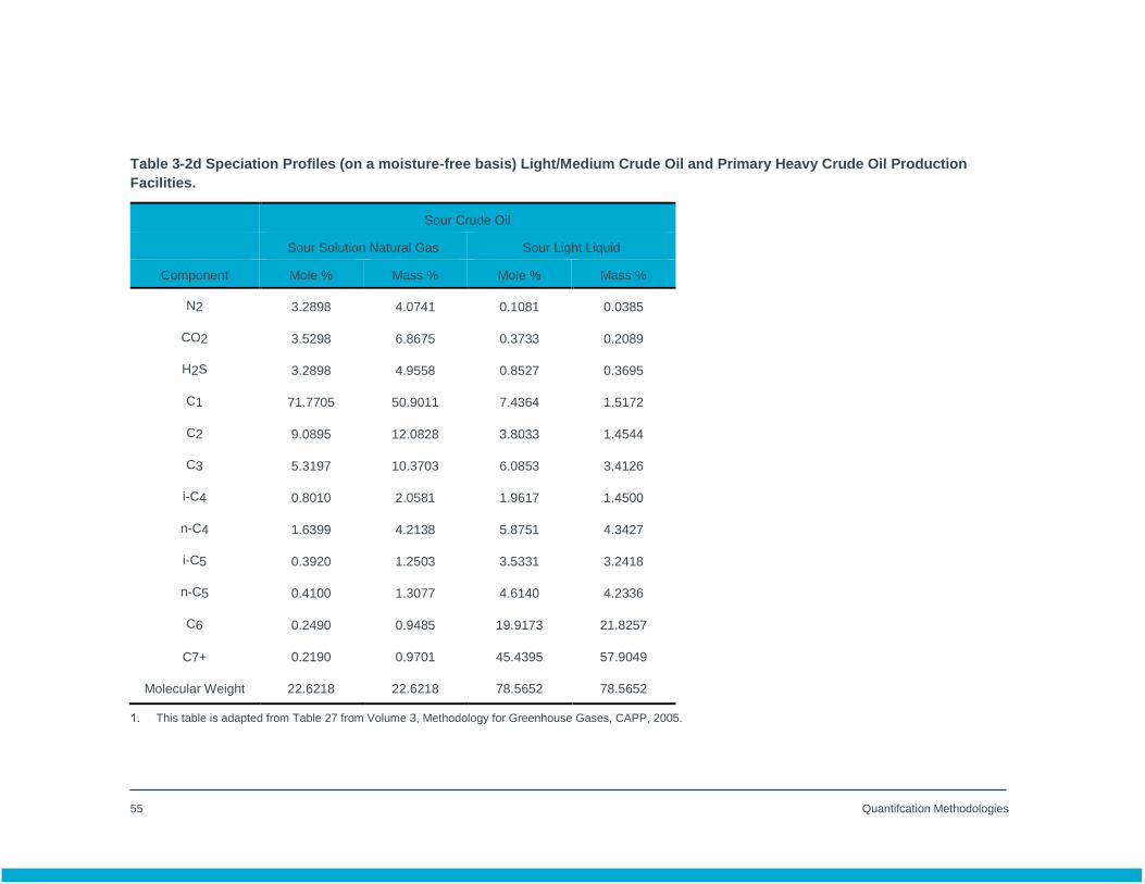
55 Quantifcation Methodologies
Table 3-2d Speciation Profiles (on a moisture-free basis) Light/Medium Crude Oil and Primary Heavy Crude Oil Production
Facilities.
Sour Crude Oil
Sour Solution Natural Gas Sour Light Liquid
Component Mole % Mass % Mole % Mass %
N2 3.2898 4.0741 0.1081 0.0385
CO2 3.5298 6.8675 0.3733 0.2089
H2S 3.2898 4.9558 0.8527 0.3695
C1 71.7705 50.9011 7.4364 1.5172
C2 9.0895 12.0828 3.8033 1.4544
C3 5.3197 10.3703 6.0853 3.4126
i-C4 0.8010 2.0581 1.9617 1.4500
n-C4 1.6399 4.2138 5.8751 4.3427
i-C5 0.3920 1.2503 3.5331 3.2418
n-C5 0.4100 1.3077 4.6140 4.2336
C6 0.2490 0.9485 19.9173 21.8257
C7+ 0.2190 0.9701 45.4395 57.9049
Molecular Weight 22.6218 22.6218 78.5652 78.5652
This table is adapted from Table 27 from Volume 3, Methodology for Greenhouse Gases, CAPP, 2005.
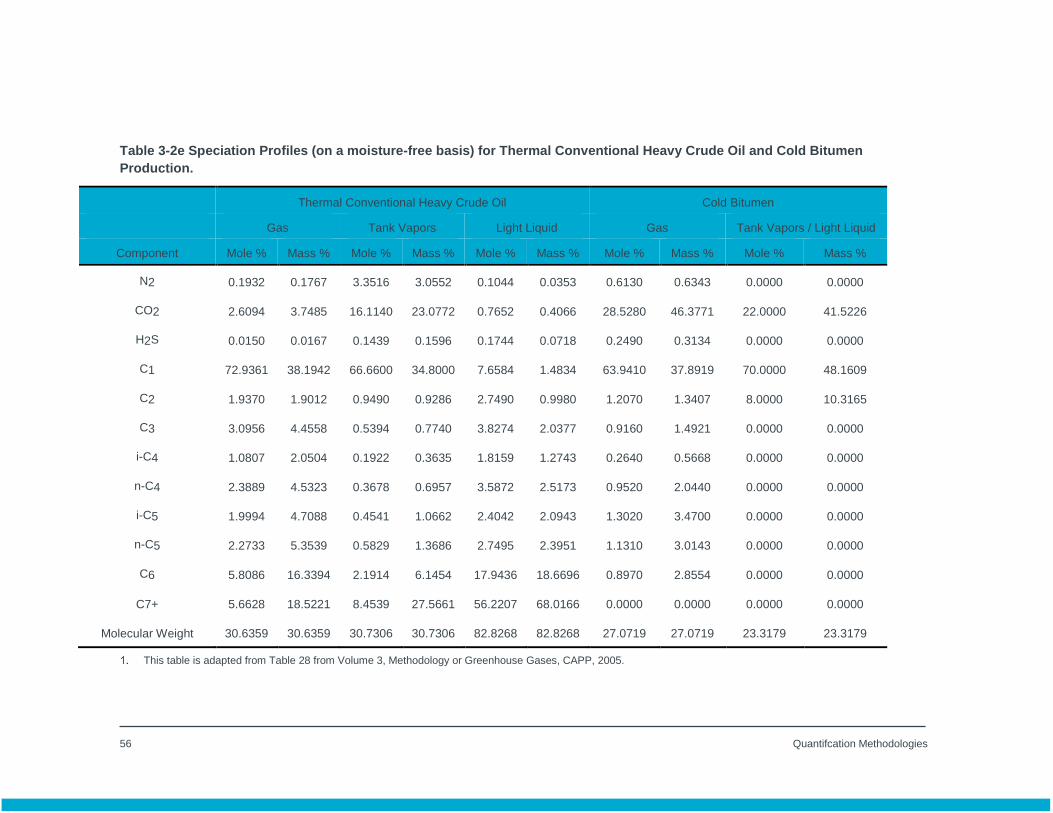
56 Quantifcation Methodologies
Table 3-2e Speciation Profiles (on a moisture-free basis) for Thermal Conventional Heavy Crude Oil and Cold Bitumen
Production.
Thermal Conventional Heavy Crude Oil Cold Bitumen
Gas Tank Vapors Light Liquid Gas Tank Vapors / Light Liquid
Component Mole % Mass % Mole % Mass % Mole % Mass % Mole % Mass % Mole % Mass %
N2 0.1932 0.1767 3.3516 3.0552 0.1044 0.0353 0.6130 0.6343 0.0000 0.0000
CO2 2.6094 3.7485 16.1140 23.0772 0.7652 0.4066 28.5280 46.3771 22.0000 41.5226
H2S 0.0150 0.0167 0.1439 0.1596 0.1744 0.0718 0.2490 0.3134 0.0000 0.0000
C1 72.9361 38.1942 66.6600 34.8000 7.6584 1.4834 63.9410 37.8919 70.0000 48.1609
C2 1.9370 1.9012 0.9490 0.9286 2.7490 0.9980 1.2070 1.3407 8.0000 10.3165
C3 3.0956 4.4558 0.5394 0.7740 3.8274 2.0377 0.9160 1.4921 0.0000 0.0000
i-C4 1.0807 2.0504 0.1922 0.3635 1.8159 1.2743 0.2640 0.5668 0.0000 0.0000
n-C4 2.3889 4.5323 0.3678 0.6957 3.5872 2.5173 0.9520 2.0440 0.0000 0.0000
i-C5 1.9994 4.7088 0.4541 1.0662 2.4042 2.0943 1.3020 3.4700 0.0000 0.0000
n-C5 2.2733 5.3539 0.5829 1.3686 2.7495 2.3951 1.1310 3.0143 0.0000 0.0000
C6 5.8086 16.3394 2.1914 6.1454 17.9436 18.6696 0.8970 2.8554 0.0000 0.0000
C7+ 5.6628 18.5221 8.4539 27.5661 56.2207 68.0166 0.0000 0.0000 0.0000 0.0000
Molecular Weight 30.6359 30.6359 30.7306 30.7306 82.8268 82.8268 27.0719 27.0719 23.3179 23.3179
This table is adapted from Table 28 from Volume 3, Methodology or Greenhouse Gases, CAPP, 2005.
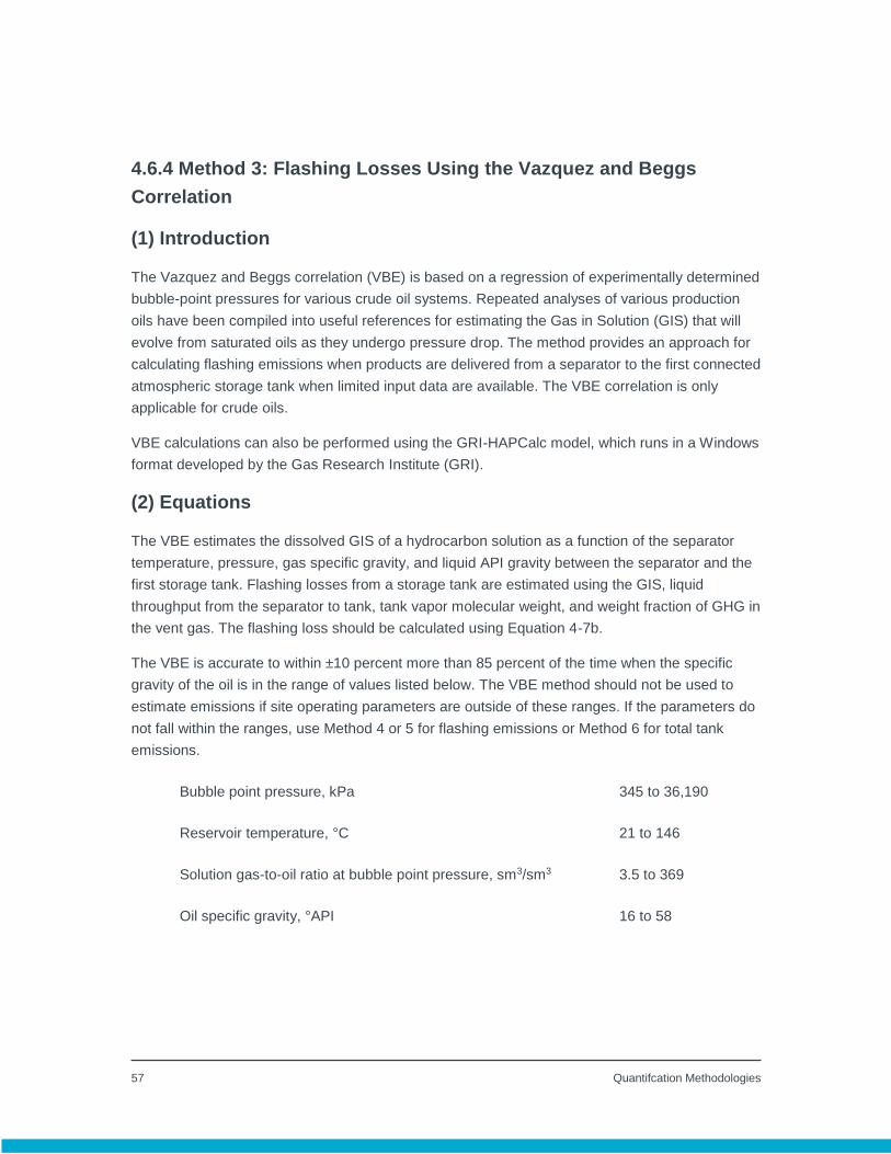
57 Quantifcation Methodologies
4.6.4 Method 3: Flashing Losses Using the Vazquez and Beggs
Correlation
(1) Introduction
The Vazquez and Beggs correlation (VBE) is based on a regression of experimentally determined
bubble-point pressures for various crude oil systems. Repeated analyses of various production
oils have been compiled into useful references for estimating the Gas in Solution (GIS) that will
evolve from saturated oils as they undergo pressure drop. The method provides an approach for
calculating flashing emissions when products are delivered from a separator to the first connected
atmospheric storage tank when limited input data are available. The VBE correlation is only
applicable for crude oils.
VBE calculations can also be performed using the GRI-HAPCalc model, which runs in a Windows
format developed by the Gas Research Institute (GRI).
(2) Equations
The VBE estimates the dissolved GIS of a hydrocarbon solution as a function of the separator
temperature, pressure, gas specific gravity, and liquid API gravity between the separator and the
first storage tank. Flashing losses from a storage tank are estimated using the GIS, liquid
throughput from the separator to tank, tank vapor molecular weight, and weight fraction of GHG in
the vent gas. The flashing loss should be calculated using Equation 4-7b.
The VBE is accurate to within ±10 percent more than 85 percent of the time when the specific
gravity of the oil is in the range of values listed below. The VBE method should not be used to
estimate emissions if site operating parameters are outside of these ranges. If the parameters do
not fall within the ranges, use Method 4 or 5 for flashing emissions or Method 6 for total tank
emissions.
Bubble point pressure, kPa 345 to 36,190
Reservoir temperature, °C 21 to 146
Solution gas-to-oil ratio at bubble point pressure, sm3/sm3 3.5 to 369
Oil specific gravity, °API 16 to 58

58 Quantifcation Methodologies
𝐺𝐻𝐺 = 𝐶 1 × 𝛾 𝑔𝑠 × 𝑝 𝐶2 × 𝑒𝑥𝑝 (𝐶 3
𝛾 0𝑇−
𝐶 4
𝑇) × 𝑄 × 𝑉𝑇𝑀 × 𝑀𝐹 𝐺𝐻𝐺 × 𝑀𝑊 𝐺𝐻𝐺
× (1 − 𝐶𝐹) × 0.001
Equation 4-7b
Where:
GHG = CH4 or CO2 mass emissions (tonnes) from storage tank in the report period.
𝛾 gs = Specific gas gravity corrected at 689.4 kpa or 100 psig with respect to air,
calculated by Equation 4-7c.
P = Absolute pressure upstream of the vessel of interest (kPaa).
T = Temperature at upstream of the vessel of interest (K).
γ ₒ = Specific gravity of the liquid hydrocarbon at final condition of the separator
with respect to water, calculated by Equation 4-7d (dimensionless).
C 1 = For 𝛾ₒ <0.876, 3.204 × 10⁻⁴; 𝛾ₒ ≥0.876, 7.803×10⁻⁴.
C 2 = For 𝛾ₒ <0.876, 1.187; 𝛾ₒ ≥0.876, 1.0937.
C 3 = For 𝛾ₒ <0.876, 1,881.24; 𝛾ₒ ≥0.876, 2,022.19.
C 4 = For 𝛾ₒ <0.876, 1,748.29; 𝛾ₒ ≥0.876, 1,879.28.
Q = Throughputs of liquid hydrocarbon in a tank (m3) for the report period.
MF GHG = CH4 or CO2 mole fraction. Measured by the facility or if unavailable, refer to
values presented in Tables 3-2a to 3-2e of Chapter 3 Fugitives.
MW GHG = Molecular weight of CH4 or CO2 (kg/kmol).
VTM = Volume to mole conversion at standard condition of 101.325 kPa and 15°C;
0.042293 kmol/m3.
𝜸𝒈𝒔 = 𝜸𝒈 [𝟏 + (𝟖. 𝟑𝟔𝟓
𝜸𝟎
− 𝟕. 𝟕𝟕𝟒) ×(𝟏. 𝟖 × 𝑻 − 𝟒𝟓𝟗. 𝟕)
𝟏𝟎𝟎𝟎× 𝐥𝐨𝐠 (
𝒑
𝟕𝟗𝟎. 𝟖𝟑)] Equation 4-7c

59 Quantifcation Methodologies
Where:
γg = Specific gravity of a gas in the upstream of a vessel at the actual
conditions, calculated by Equation 4-7e (dimensionless).
𝜸 𝟎 =𝟏𝟒𝟏. 𝟓
𝟏𝟑𝟏. 𝟓 + °𝑨𝑷𝑰 Equation 4-7d
Where:
◦API = API gravity of product in the separator before the first storage tank.
𝜸𝒈 =𝑴𝑾 𝒔𝒈
𝑴𝑾 𝒂𝒊𝒓
Equation 4-7e
Where:
MW sg = Molecular weight of solution gas at standard temperature and pressure
conditions.
MW air = Molecular weight of air, (28.96 g/mol) at standard temperature and
pressure conditions.
(3) Data requirements
A facility may determine the composition based on process knowledge and/or engineering
estimates or use default compositions as presented in Tables 3-2a to 3-2e in Chapter 3.
Method 4: Flashing Losses using Models/Simulations or Engineering
Estimation
(1) Introduction
For tanks storing non-crude hydrocarbons, Method 3 may not be appropriate for use. Facilities
may use other models, simulations, or engineering estimates to quantify flashing losses when the
contents from the separator or non-separator equipment enters an atmospheric pressure storage
tank. Various methods are available to estimate flashing losses as listed below.
60 Quantifcation Methodologies
(2) Methods
Peng-Robinson Equation of State (for flashing emissions only).
Process simulators such as HYSIM, HYSYS, WINSIM, PROSIM.
Engineering estimate based on process or emission specific data.
(3) Data requirements
Site specific process and operational conditions should be used for modelling, simulations or
engineering estimates.
Facilities are required to document methodologies, supporting data, and assumptions used to
calculate the emissions.
4.6.6 Method 5: Flashing Losses Using the Measured GIS Method
(1) Introduction
The GIS should be a measured value reflecting the flashing emissions due to the pressure drop
from the up stream separator to the first storage tank. An extended hydrocarbon analysis of the
flash gas from the sample should also be conducted to determine the methane concentrations in
the tank’s flashing emissions.
(2) Equations
The equations for flashing losses are outlined in Section 4.2.3.
(3) Data requirements
The data requirements are outlined in Section 4.2.3.
4.6.7 Method 6: Total Tank Emissions Using Peng-Robinson (PR)
Equation of State (EOS)
(1) Introduction
Models based on the Peng-Robinson (PR) Equation of State (EOS) may be used to calculate the
total tank emissions including flashing, breathing and working losses from fixed-and floating-roof
storage tanks. EOS is a mathematical equation relating thermodynamic variables such as
pressure, temperature, and volume of a specific material in thermodynamic equilibrium.

61 Quantifcation Methodologies
The emissions calculated can represent the total VOCs or specific GHG depending on the
parameters used in the calculation.
(2) Equations
If total VOCs are determined from the modelling, calculate the CH4 or CO2 emissions using the
Equation 4-7a and follow the data requirement in Section 4.5.4 for tank vapor analysis.
If total GHGs are determined from the modelling, calculate the CH4 or CO2 emissions using
Equation 4-8 based on the uncontrolled CO2 and CH4 and apply the control efficiency of the
emissions recovery system.
𝐺𝐻𝐺 = ∑ ∑[𝑀𝑎𝑠𝑠 𝐺𝐻𝐺,𝑖,𝑗 × (1 − 𝐶𝐹 𝑖,𝑗)]
𝐼
𝑖=0
𝐽
𝑗=0
Equation 4-8
Where:
GHG = CH4 or CO2 mass emissions (tonnes) in the report period.
i = Tank identifier.
I = Number of tanks holding products in the report period.
j = Type of product.
J = Number of products in the report period.
Mass GHG,i,j = CO2 or CH4 mass emissions (tonnes) for product i in tank j in the
report period. This value is derived from the modelling using the
Peng-Robinson Equation of State.
CF = Control factor (dimensionless fraction).
(3) Data requirements
A facility should follow EOS to quantify model input parameters.
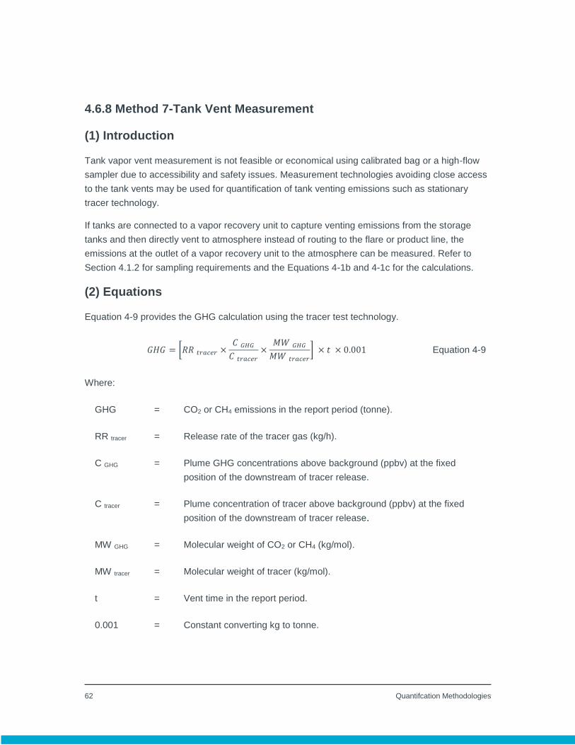
62 Quantifcation Methodologies
4.6.8 Method 7-Tank Vent Measurement
(1) Introduction
Tank vapor vent measurement is not feasible or economical using calibrated bag or a high-flow
sampler due to accessibility and safety issues. Measurement technologies avoiding close access
to the tank vents may be used for quantification of tank venting emissions such as stationary
tracer technology.
If tanks are connected to a vapor recovery unit to capture venting emissions from the storage
tanks and then directly vent to atmosphere instead of routing to the flare or product line, the
emissions at the outlet of a vapor recovery unit to the atmosphere can be measured. Refer to
Section 4.1.2 for sampling requirements and the Equations 4-1b and 4-1c for the calculations.
(2) Equations
Equation 4-9 provides the GHG calculation using the tracer test technology.
𝐺𝐻𝐺 = [𝑅𝑅 𝑡𝑟𝑎𝑐𝑒𝑟 ×𝐶 𝐺𝐻𝐺
𝐶 𝑡𝑟𝑎𝑐𝑒𝑟
×𝑀𝑊 𝐺𝐻𝐺
𝑀𝑊 𝑡𝑟𝑎𝑐𝑒𝑟
] × 𝑡 × 0.001 Equation 4-9
Where:
GHG = CO2 or CH4 emissions in the report period (tonne).
RR tracer = Release rate of the tracer gas (kg/h).
C GHG = Plume GHG concentrations above background (ppbv) at the fixed
position of the downstream of tracer release.
C tracer = Plume concentration of tracer above background (ppbv) at the fixed
position of the downstream of tracer release.
MW GHG = Molecular weight of CO2 or CH4 (kg/mol).
MW tracer = Molecular weight of tracer (kg/mol).
t = Vent time in the report period.
0.001 = Constant converting kg to tonne.

63 Quantifcation Methodologies
(3) Data requirements
Data requirements are prescribed in Section 4.1.2.
Tracer test should be performed during representative operating conditions for the tanks.
The tracer test and composition of tank vapor including CH4 and CO2 should be measured at
least once every 3 years for each storage product. It is acceptable to take one measurement
if there are multiple tanks with the same physical parameters (including color, roof
configuration, dimensions etc.), operational condition and contains the same product. If there
is a product change or operational condition change, a new test and measurement should be
conducted for the tank(s).
4.7 Routine Venting-Pneumatic Control Instruments
4.7.1 Introduction
Pneumatic instruments mean automated flow control instruments powered by pressurized natural
gas and used for maintaining a process condition such as liquid level, pressure, delta-pressure
and temperature.
Venting can occur from gas-actuated pneumatic control loops, which can include controllers,
transmitters, positioners and transducers. All emissions from static, transient and dynamic control
instruments are released to the atmosphere if vent emissions control equipment is not installed.
The vent gas from pneumatic control instruments can be collected and recovered and are often
piped away in a common vent line or sent to a flare stack with a control system. However, vent
emissions may still be released from inefficiencies in the operation of emissions control systems.
4.7.2 Tier 1-Generic Vent Rates
(1) Introduction
Generic emission factors are distinguished by pneumatic instrument type for UOG facilities. For
other facilities, emission factors are classified by high bleed and low bleed along with intermittent
or continuous bleed. The classification of the pneumatic instruments are described in the
following:
High-bleed pneumatic instruments means part of the gas power stream which is regulated by
the process condition flows to a valve actuator controller where it vents (bleeds) to the
atmosphere at a rate in excess of 0.17 standard cubic meters per hour.

64 Quantifcation Methodologies
Low-bleed pneumatic instruments mean part of the gas power stream, which is regulated by
the process condition flows to a valve actuator controller where it vents (bleeds) to the
atmosphere at a rate equal to or less than 0.17 standard cubic meters per hour.
Intermittent-bleed (high and low) pneumatic are snap-acting or throttling instruments that
discharge the full volume of the actuator intermittently when control action is necessary, but
does not bleed continuously.
(2) Equations
Calculate GHG emissions using Equation 4-10.
𝑮𝑯𝑮 = 𝝆 𝑮𝑯𝑮 × 𝟎. 𝟎𝟎𝟏 × ∑ 𝑽𝑹 𝒊 × 𝒕 𝒊 × (𝟏 − 𝑪𝑭 𝒊) × 𝑴𝑭 𝑮𝑯𝑮,𝒊
𝒏
𝒊=𝟏
Equation 4-10
Where:
GHG = CH4 or CO2 mass emissions from pneumatic control device venting
(tonnes) in the report period.
i = Pneumatic device identifier.
n = Number of pneumatic instruments in the report period.
VR i = Average vent rate for the device i (m3/hour/device) at the standard
condition in Table 4-1a and 4-1b.
t i = Operating time of the instrument i in the report period (hours).
CF i = Control factor (dimensionless fraction) for pneumatic device i.
MF GHG.i = Mole fraction of CO2 or CH4 in vented gas. Refer to Table 17-3 of Chapter
17 for natural gas composition sampling requirements.
GHG = Density of CO2 or CH4 at standard conditions (CO2 = 1.861 kg/sm3;
CH4 = 0.6785 kg/sm3).
0.001 = Mass conversion factor (tonne/kg).
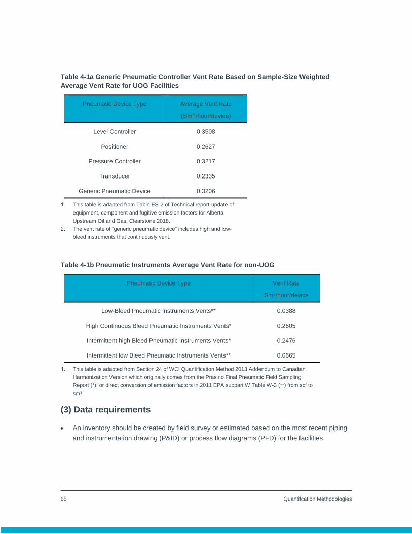
65 Quantifcation Methodologies
Table 4-1a Generic Pneumatic Controller Vent Rate Based on Sample-Size Weighted
Average Vent Rate for UOG Facilities
Pneumatic Device Type Average Vent Rate
(Sm3 /hour/device)
Level Controller 0.3508
Positioner 0.2627
Pressure Controller 0.3217
Transducer 0.2335
Generic Pneumatic Device 0.3206
This table is adapted from Table ES-2 of Technical report-update of
equipment, component and fugitive emission factors for Alberta
Upstream Oil and Gas, Clearstone 2018.
The vent rate of “generic pneumatic device” includes high and low-
bleed instruments that continuously vent.
Table 4-1b Pneumatic Instruments Average Vent Rate for non-UOG
Pneumatic Device Type Vent Rate
Sm3/hour/device
Low-Bleed Pneumatic Instruments Vents** 0.0388
High Continuous Bleed Pneumatic Instruments Vents* 0.2605
Intermittent high Bleed Pneumatic Instruments Vents* 0.2476
Intermittent low Bleed Pneumatic Instruments Vents** 0.0665
This table is adapted from Section 24 of WCI Quantification Method 2013 Addendum to Canadian
Harmonization Version which originally comes from the Prasino Final Pneumatic Field Sampling
Report (*), or direct conversion of emission factors in 2011 EPA subpart W Table W-3 (**) from scf to
sm3.
(3) Data requirements
An inventory should be created by field survey or estimated based on the most recent piping
and instrumentation drawing (P&ID) or process flow diagrams (PFD) for the facilities.
66 Quantifcation Methodologies
The facility should update the inventory whenever there are changes in equipment (replaced,
added or decommissioned) at the facility.
Information regarding the make and model, pneumatic instrument type (positioner,
transducer, pressure or level controller), actuation frequency of level controllers should be
documented.
Information regarding pneumatic instrument type (low-bleed, high continuous bleed,
intermittent high/low bleed) should be documented for transmission and underground storage
and distribution facilities.
Facilities are required to follow gas sampling frequencies prescribed in Table 17.3 of Chapter
17.
Vent gas properties such as gas composition must be measured using an analytical method
prescribed in Section 17.2.3 of Chapter 17.
Facilities may use the fuel gas composition if it is considered to be representative of the
vented gas.
4.7.3 Tiers 2 and 3-Specific Manufacturer and Model Vent Rate or
Calculated Based on Correlation
(1) Introduction
The published venting rates are generated based on the average vent rates for specific
pneumatic control device manufacturers and models. The vent rates are further distinguished into
high bleed or low bleed and continuous or intermittent operations.
(2) Equations
Equation 4-10 should be used to calculate the GHG vent emissions using the vent rates in Tables
4-2a or 4-2b. However, the average vent rate in Table 4-2a for the specific manufacturer and
model of device must be considered first since the data provided in this table were developed
based on extensive field surveys of oil gas facilities in Alberta and British Columbia. If a device
manufacturer and model are not listed in the Table 4-2a, use the vent rate based on the device’s
manufacturer vent rate in Table 4-2b.
𝑽𝑹 𝒊 = 𝒎 × 𝑺𝑷 𝒊 Equation 4-11
67 Quantifcation Methodologies
Where:
VR i = Average vent rate determined by the manufacturer and model i and
operating condition of pneumatic instrument at the standard condition
(Sm3/hour).
m = Supply pressure coefficient in Table 4-2a (m3/hour/kpa gauge).
SP i = Supply pressure of controller i to the instrument (kpa gauge).
The vent rate should be calculated using Equation 4-11 and data provided in Table 4-2a for the
following scenarios in the preferable order of accuracy:
Use specific model coefficient in Table 4-2a if the manufacturer, model and operational
pressure are available;
Use a vent rate based on the device manufacturer and model provided in the last column of
the Table 4-2a (m3/hour/device) if the manufacturer and model are available, but the
operational pressure is not known; or
Use generic high bleed and low bleed coefficients from Table 4-2a if operational pressures
are available, but the pneumatic manufacturer and model type are not known.
If the manufacturer and model are not available in the Table 4-2a, use the manufacturer vent rate
in Table 4-2b. These manufacturer vent rates are based on manufacturer lab testing and may not
reflect actual field conditions. The vent rates should be selected as follows:
If the manufacturer and model are listed in Table 4-2b, a manufacturer-specified emission
rate should be selected which best represents the site operating conditions: continuous or
intermittent;
If the manufacturer and model are not listed in Table 4-2b, choose a vent rate in the table that
is similar to the model used at the facility based on process knowledge; or
If a similar manufacturer and model can not be found in Table 4-2b, use the highest emission
rate available for the manufacturer of the pneumatic device.
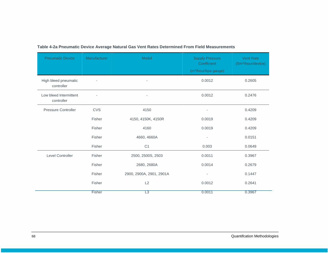
68 Quantifcation Methodologies
Table 4-2a Pneumatic Device Average Natural Gas Vent Rates Determined From Field Measurements
Pneumatic Device Manufacturer Model Supply Pressure
Coefficient
(m3/hour/kpa gauge)
Vent Rate
(Sm3/hour/device)
High bleed pneumatic
controller
- - 0.0012 0.2605
Low bleed Intermittent
controller
- - 0.0012 0.2476
Pressure Controller CVS 4150 - 0.4209
Fisher 4150, 4150K, 4150R 0.0019 0.4209
Fisher 4160 0.0019 0.4209
Fisher 4660, 4660A - 0.0151
Fisher C1 0.003 0.0649
Level Controller Fisher 2500, 2500S, 2503 0.0011 0.3967
Fisher 2680, 2680A 0.0014 0.2679
Fisher 2900, 2900A, 2901, 2901A - 0.1447
Fisher L2 0.0012 0.2641
Fisher L3 0.0011 0.3967
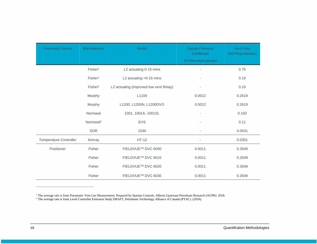
69 Quantifcation Methodologies
Pneumatic Device Manufacturer Model Supply Pressure
Coefficient
(m3/hour/kpa gauge)
Vent Rate
(Sm3/hour/device)
Fisher1 L2 actuating 0-15 mins - 0.75
Fisher1 L2 actuating >0-15 mins - 0.19
Fisher2 L2 actuating (improved low vent Relay) - 0.10
Murphy L1100 0.0012 0.2619
Murphy L1200, L1200N, L1200DVO 0.0012 0.2619
Norriseal 1001, 1001A, 1001XL - 0.193
Norriseal2 EVS - 0.11
SOR 1530 - 0.0531
Temperature Controller Kimray HT-12 - 0.0351
Positioner Fisher FIELDVUETM DVC 6000 0.0011 0.2649
Fisher FIELDVUETM DVC 6010 0.0011 0.2649
Fisher FIELDVUETM DVC 6020 0.0011 0.2649
Fisher FIELDVUETM DVC 6030 0.0011 0.2649
1 The average rate is from Pneumatic Vent Gas Measurement. Prepared by Spartan Controls, Alberta Upstream Petroleum Research (AUPR). 2018. 2 The average rate is from Level Controller Emission Study DRAFT, Petroleum Technology Alliance of Canada (PTAC). (2018).
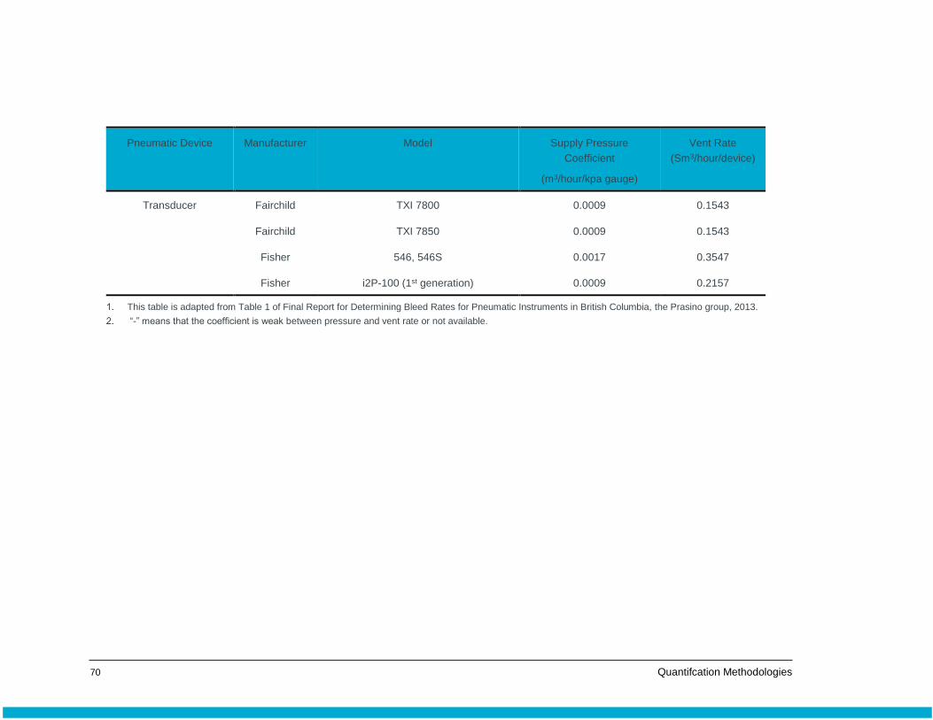
70 Quantifcation Methodologies
Pneumatic Device Manufacturer Model Supply Pressure
Coefficient
(m3/hour/kpa gauge)
Vent Rate
(Sm3/hour/device)
Transducer Fairchild TXI 7800 0.0009 0.1543
Fairchild TXI 7850 0.0009 0.1543
Fisher 546, 546S 0.0017 0.3547
Fisher i2P-100 (1st generation) 0.0009 0.2157
This table is adapted from Table 1 of Final Report for Determining Bleed Rates for Pneumatic Instruments in British Columbia, the Prasino group, 2013.
“-” means that the coefficient is weak between pressure and vent rate or not available.

71 Quantifcation Methodologies
Table 4-2b Average Manufacturer Vent Rates for Pneumatic Instruments1
Controller Model Supply Pressure
(psi)
Manufacturer Vent Rate
(sm3/h/device)2
Pressure Controllers
Ametek Series 40 20 0.22
35 0.22
Bristol Babcock Series 5453-Model 10F 20 0.11
35 0.11
Bristol Babcock Series 5455-Model 624-III 20 0.07
35 0.11
Bristol Babcock Series 502 A / D (recording
controller)
20 0.22
35 0.22
Dynaflo 4000LB 20 0.06
35 0.09
Fisher 4100 Series (Large Orifice) 20 1.83
35 1.83
Fisher 4194 Series (Differential Pressure) 20 0.13
35 0.18
Fisher 4195 20 0.13
35 0.18
Foxboro 43AP 20 0.66
35 0.66
ITT Barton 338 20 0.22
35 0.22
ITT Barton 335P 20 0.22
35 0.22

72 Quantifcation Methodologies
Controller Model Supply Pressure
(psi)
Manufacturer Vent Rate
(sm3/h/device)2
Natco CT 20 1.28
35 1.28
Transducers
Bristol Babcock Series 9110-00A 20 0.02
35 0.02
Fisher i2P-100LB 20 0.08
35 0.11
Fisher 646 20 0.04
35 0.04
Fisher 846 20 0.04
35 0.04
Level Controllers
Dynaflo 5000 20 0
35 0
Fisher 2660 Series 20 0.04
35 0.04
Fisher 2100 Series 20 0.04
35 0.04
Fisher L2sj 20 0.01
35 0.02
Invalco CT Series 20 0.05
35 1.46
Wellmark 2001 20 0.01
35 0.01

73 Quantifcation Methodologies
Controller Model Supply Pressure
(psi)
Manufacturer Vent Rate
(sm3/h/device)2
Positioners
Fisher 3582 20 0.51
35 0.66
Fisher 3661 20 0.32
35 0.44
Fisher 3590 (Electro-pneumatic) 20 0.88
35 1.32
Fisher 3582i (Electro-pneumatic) 20 0.63
35 0.88
Fisher 3620J (Electro-pneumatic) 20 0.66
35 1.28
Fisher 3660 20 0.22
35 0.29
Fisher FIELDVUE DVC5000 20 0.37
35 0.55
Fisher FIELDVUE DVC6200 (standard) 20 0.51
80 1.79
Fisher FIELDVUE DVC6200 (low bleed) 20 0.08
80 0.25
Masoneilan SVI Digital 20 0.04
35 0.04
Moore Products – Model 750P 20 0
35 1.53
Moore Products – 73 – B PtoP 20 1.32

74 Quantifcation Methodologies
Controller Model Supply Pressure
(psi)
Manufacturer Vent Rate
(sm3/h/device)2
35 0
PMV D5 Digital 20 0.04
35 0.04
Sampson 3780 Digital 20 0.04
35 0.04
Siemens PS2 20 0.04
35 0.04
VRC Model VP7000 PtoP 20 0.04
35 0.04
This table is adapted from the Quantification Protocol for Greenhouse Gas Emission Reductions from Pneumatic
Devices, version 2.0, January 25, 2017 and Alberta Energy Regulator's Manual 015, December 2018.
Manufacturer vent rates were multipled by 1.29 to convert volumes from total air to total fuel gas.

75 Quantifcation Methodologies
(3) Data requirements
An inventory should be created by field survey or estimated based on the most recent piping
and instrumentation drawing (P&ID) or process flow diagrams (PFD) for the facilities.
The facility should update the inventory whenever there are changes in equipment (replaced,
added or decommissioned) at the facility.
Information regarding manufacturer, model type, and operating conditions (continuous or
intermittent) must be collected and documented.
Facilities are required to follow gas sampling frequencies prescribed in Table 17.3 of Chapter
17.
Vent gas properties such as gas composition must be measured using an analytical method
prescribed in Section 17.2.3 of Chapter 17.
Facilities may use the fuel gas composition if it is considered to be representative of the
vented gas.
4.7.4 Tier 4-Direct Measurement
(1) Introduction
Direct measurements may be conducted periodically or continuously.
Periodic measurement may miss dynamic bleeding events and the facility would have to conduct
other measurements to capture dynamic bleeding. Continuous measurements can capture
vented emissions in full bleed cycle.
(2) Equations
Equation 4-1b or 4-1c can be used to calculate the vented emissions from direct measurements.
The vent rate is based on the actual field measurement of the pneumatic instruments either from
periodic or continuous measurements.
(3) Data requirements
Refer to Section 4.1.2 for data requirements.
Periodic measurements must be conducted on a quarterly basis at minimum.
76 Quantifcation Methodologies
The measurement must capture both the static and dynamic bleed rates for pneumatic
instruments.
Facilities are required to follow gas sampling frequencies prescribed in Table 17.3 of Chapter
17.
Vent gas properties such as gas composition must be measured using an analytical method
prescribed in Section 17.2.3 of Chapter 17.
Facilities may use the fuel gas composition if it is considered to be representative of the
vented gas.
4.8 Routine Venting-Pneumatic Pumps
4.8.1 Introduction
Pneumatic pumps use the force of compressed gases to generate mechanical effects, which
drive the pump plunger and inject liquid chemicals such as corrosion inhibitors, de-foamers or
anti-foamers, detergents, methanol, and emulsifiers or de-emulsifiers into the pressurized system
(pipeline or wells) for specific applications. The expanded supply gas is then vented to
atmosphere (or into a collection system) and the cycle repeated.
4.8.2 Tier 1-Default Vent Rates
(1) Introduction
The method uses the generic vent rates for diaphragm and piston pumps. Emission factors for
several models are provided as well.
(2) Equations
Calculate CH4 or CO2 emissions using Equation 4-10 for pneumatic instruments.
If the pneumatic pump’s manufacturer and models are not available, the generic vent rates for
pneumatic piston and diaphragm pumps should be used. Several pump models are provided in
Table 4-3 (m3/hour/pump).

77 Quantifcation Methodologies
Table 4-3 Pneumatic Pump Average Natural Gas Vent Rates Based on Field Measurements
Pneumatic Device Average Vent Rate
(Sm3/hour/pump)
Generic piston pumps 0.5917
Generic diaphragm pumps 1.0542
Morgan HD312 1.1292
Texsteam 5100 0.9670
Williams P125 0.4098
Williams P250 0.8022
Williams P500 0.6969
This table is adapted from Table 11 of the final report for determining bleed rates for pneumatic instruments in British
Columbia, the Prasino group, 2013.
(3) Data requirements
An inventory must be done by field survey once and repeated following any changes to the
inventory.
The facility should update the inventory whenever there are changes in equipment (replaced,
added or decommissioned) at the facility.
Information regarding to the pump types (piston or diaphragm), manufacturer and model
types must be collected and documented.
Facilities may use the fuel gas composition if it is considered to be representative of the
vented gas.
Facilities are required to follow gas sampling frequencies prescribed in Table 17.3 of Chapter
17.
Fuel properties such as gas composition must be measured using an analytical method
prescribed in Section 17.2.3 of Chapter 17.
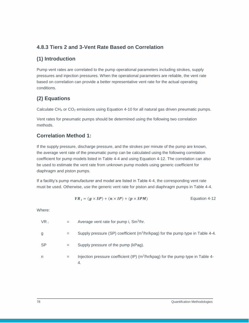
78 Quantifcation Methodologies
4.8.3 Tiers 2 and 3-Vent Rate Based on Correlation
(1) Introduction
Pump vent rates are correlated to the pump operational parameters including strokes, supply
pressures and injection pressures. When the operational parameters are reliable, the vent rate
based on correlation can provide a better representative vent rate for the actual operating
conditions.
(2) Equations
Calculate CH4 or CO2 emissions using Equation 4-10 for all natural gas driven pneumatic pumps.
Vent rates for pneumatic pumps should be determined using the following two correlation
methods.
Correlation Method 1:
If the supply pressure, discharge pressure, and the strokes per minute of the pump are known,
the average vent rate of the pneumatic pump can be calculated using the following correlation
coefficient for pump models listed in Table 4-4 and using Equation 4-12. The correlation can also
be used to estimate the vent rate from unknown pump models using generic coefficient for
diaphragm and piston pumps.
If a facility’s pump manufacturer and model are listed in Table 4-4, the corresponding vent rate
must be used. Otherwise, use the generic vent rate for piston and diaphragm pumps in Table 4-4.
𝑽𝑹 𝒊 = (𝒈 × 𝑺𝑷) + (𝒏 × 𝑰𝑷) + (𝒑 × 𝑺𝑷𝑴) Equation 4-12
Where:
VR i = Average vent rate for pump i, Sm3/hr.
g = Supply pressure (SP) coefficient (m3/hr/kpag) for the pump type in Table 4-4.
SP = Supply pressure of the pump (kPag).
n = Injection pressure coefficient (IP) (m3/hr/kpag) for the pump type in Table 4-
4.

79 Quantifcation Methodologies
IP = Injection pressure of the pump (kPag).
p = Strokes per minute coefficient (m3/hr/kpag) for the pump type in Table 4-4.
SPM = Strokes per minute of the pump (strokes/minute).
Table 4-4: Coefficients for Determining Pneumatic Pump Average Emission Rates
Pump Type Supply Pressure
Coefficient (g)
(m3/hr/kpag)
Injection Pressure
Coefficient (n)
(m3/hr/kpag)
Strokes per minute
Coefficient (p)
(m3/hr/kpag)
Generic diaphragm
pump
0.00202 0.000059 0.0167
Generic piston pump 0.00500 0.000027 0.0091
Morgan HD312 0.00418 0.000034 0.0073
Texsteam 5100 0.00030 0.000034 0.0207
Williams P125 0.00019 0.000024 0.0076
Williams P250 0.00096 0.000042 0.0079
Williams P500 0.00224 -0.000031 0.0046
This table is adapted from Table 11 of the final report for determining bleed rates for pneumatic
instruments in British Columbia, the Prasino group, 2013.
Correlation Method 2:
Pneumatic pump manufacturers commonly publish charts and graphs in product brochure that
can be used to determine the gas consumption for each make and model of pump under a variety
of operating conditions. The following method was derived data collected from multiple device
manufacturers.
Use Equation 4-13 to calculate GHG emissions and Equation 4-13a to calculate pump vent rate.
𝑮𝑯𝑮 = ∑ ∑ 𝑸 𝑪,𝒋 × 𝑽𝑹 𝒋 × (𝟏 − 𝑪𝑭)
𝒎
𝒋=𝟏
𝒏
𝒊=𝟏
× 𝑴𝑭 𝑮𝑯𝑮 × 𝝆 𝑮𝑯𝑮 × 𝟎. 𝟎𝟎𝟏 Equation 4-13
80 Quantifcation Methodologies
Where:
GHG = CH4 or CO2 mass emissions (tonnes) from pneumatic pump venting in
the report period.
Q C,j = Volume of liquid chemical injected by pump j (litres).
j = Pump type identifier.
i = Number of the pump identifier.
m = Number of pump types.
n = Number of pumps for each type of pump.
CF = Emission control factor (dimensionless).
VR j = Natural gas-driven pneumatic pump, j, venting rate (sm3/liter/pump)
determined from the correlation in Equation 4-13a.
MF GHG = Mole fraction of CO2 or CH4 in vented gas.
GHG = Density of CO2 or CH4 at standard conditions (CO2 = 1.861 kg/sm3;
CH4 = 0.6785 kg/sm3).
0.001 = Mass conversion factor (tonne/kg).
𝑽𝑹 𝒋 = 𝒄 × 𝑪𝑰𝑷𝟐 + 𝒅 × 𝑪𝑰𝑷 + 𝒆 Equation 4-13a
Where:
VR j = Natural gas-driven pneumatic pump, j, vent rate per pumping a liter of
liquid (Sm3/liter/pump).
CIP = Chemical injection pressure (pipeline pressure) (kPa gauge).
C = Manufacturer CIP2 coefficient c provided in Table 4-5.
D = Manufacturer CIP1 coefficient d provided in Table 4-5.
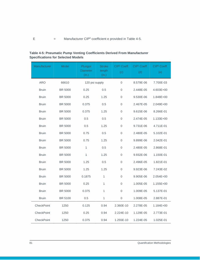
81 Quantifcation Methodologies
E = Manufacturer CIP0 coefficient e provided in Table 4-5.
Table 4-5: Pneumatic Pump Venting Coefficients Derived From Manufacturer
Specifications for Selected Models
Manufacturer Model Plunger
Diameter
(in.)
Stroke
length
(in.)
CIP2 Coeff.
(c)
CIP1 Coeff.
(d)
CIP0 Coeff.
(e)
ARO 66610 120 psi supply 0 8.579E-06 7.700E-03
Bruin BR 5000 0.25 0.5 0 2.448E-05 4.603E+00
Bruin BR 5000 0.25 1.25 0 9.530E-06 1.848E+00
Bruin BR 5000 0.375 0.5 0 2.467E-05 2.049E+00
Bruin BR 5000 0.375 1.25 0 9.615E-06 8.266E-01
Bruin BR 5000 0.5 0.5 0 2.474E-05 1.133E+00
Bruin BR 5000 0.5 1.25 0 9.731E-06 4.711E-01
Bruin BR 5000 0.75 0.5 0 2.480E-05 5.102E-01
Bruin BR 5000 0.75 1.25 0 9.899E-06 2.042E-01
Bruin BR 5000 1 0.5 0 2.480E-05 2.868E-01
Bruin BR 5000 1 1.25 0 9.932E-06 1.150E-01
Bruin BR 5000 1.25 0.5 0 2.496E-05 1.821E-01
Bruin BR 5000 1.25 1.25 0 9.923E-06 7.243E-02
Bruin BR 5000 0.1875 1 0 9.905E-06 2.054E+00
Bruin BR 5000 0.25 1 0 1.005E-05 1.155E+00
Bruin BR 5000 0.375 1 0 1.009E-05 5.137E-01
Bruin BR 5100 0.5 1 0 1.008E-05 2.887E-01
CheckPoint 1250 0.125 0.94 2.360E-10 2.278E-05 1.184E+00
CheckPoint 1250 0.25 0.94 2.224E-10 1.129E-05 2.773E-01
CheckPoint 1250 0.375 0.94 1.255E-10 1.224E-05 1.025E-01

82 Quantifcation Methodologies
Manufacturer Model Plunger
Diameter
(in.)
Stroke
length
(in.)
CIP2 Coeff.
(c)
CIP1 Coeff.
(d)
CIP0 Coeff.
(e)
CheckPoint 1250 0.5 0.94 -1.266E-12 1.190E-05 7.104E-02
CheckPoint 1500 0.5 1 4.069E-11 2.733E-05 5.143E-01
CheckPoint 1500 0.75 1 1.335E-10 1.945E-05 1.729E-01
CheckPoint 1500 1 1 -9.817E-11 2.083E-05 1.123E-01
CheckPoint LPX-04 0.25 0 0 3.464E-01
CheckPoint LPX-08 0.125 0 0 1.409E+00
Linc 84T-10-x1 0.1875 1 0 1.513E-05 3.872E-01
Linc 84T-11-x1 0.25 1 0 1.071E-05 1.646E-01
Linc 84T-11-x2 0.25 1 0 1.190E-05 2.925E-01
Linc 84T-12-x2 0.5 1 0 1.190E-05 7.313E-02
Linc 84T-12-x4 0.5 1 0 1.058E-05 1.300E-01
Linc 84T-14-x4 1 1 0 1.134E-05 3.250E-02
Linc 87TA-11-x1 1 1 0 9.921E-06 8.545E-02
Linc 85T-10 0.25 1 0 1.498E-05 1.648E-01
Linc 85T-11 0.5 1 0 1.512E-05 7.393E-02
Morgan HD187-3K-
TR2
0.5 -3.059E-11 5.192E-05 3.526E-01
Morgan HD187-TR2 0.5 -1.049E-09 7.424E-05 2.494E-03
Morgan HD312-3K-
TR2
1 -4.013E-25 2.558E-05 1.058E-01
Morgan HD312-K5-
TR2
1 -2.368E-12 2.545E-05 2.546E-01
Morgan HD312-TR2 1 2.655E-09 2.198E-05 -3.868E-03
SandPiper G05 0.5 7.635E-09 2.563E-05 6.379E-03
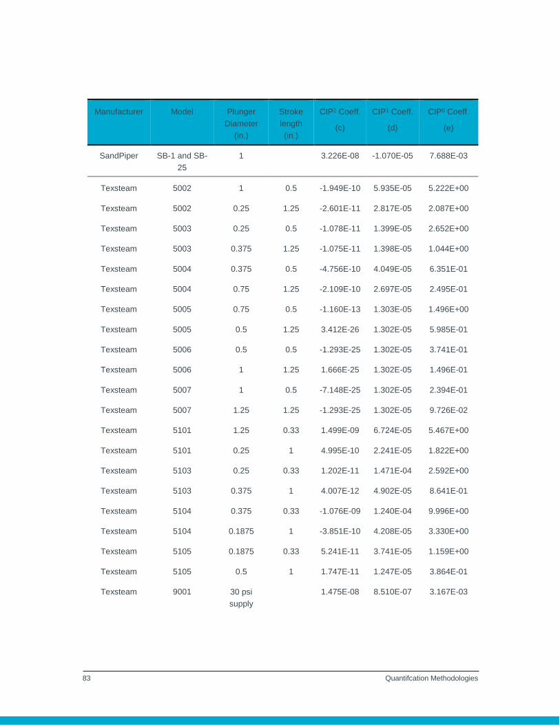
83 Quantifcation Methodologies
Manufacturer Model Plunger
Diameter
(in.)
Stroke
length
(in.)
CIP2 Coeff.
(c)
CIP1 Coeff.
(d)
CIP0 Coeff.
(e)
SandPiper SB-1 and SB-
25
1 3.226E-08 -1.070E-05 7.688E-03
Texsteam 5002 1 0.5 -1.949E-10 5.935E-05 5.222E+00
Texsteam 5002 0.25 1.25 -2.601E-11 2.817E-05 2.087E+00
Texsteam 5003 0.25 0.5 -1.078E-11 1.399E-05 2.652E+00
Texsteam 5003 0.375 1.25 -1.075E-11 1.398E-05 1.044E+00
Texsteam 5004 0.375 0.5 -4.756E-10 4.049E-05 6.351E-01
Texsteam 5004 0.75 1.25 -2.109E-10 2.697E-05 2.495E-01
Texsteam 5005 0.75 0.5 -1.160E-13 1.303E-05 1.496E+00
Texsteam 5005 0.5 1.25 3.412E-26 1.302E-05 5.985E-01
Texsteam 5006 0.5 0.5 -1.293E-25 1.302E-05 3.741E-01
Texsteam 5006 1 1.25 1.666E-25 1.302E-05 1.496E-01
Texsteam 5007 1 0.5 -7.148E-25 1.302E-05 2.394E-01
Texsteam 5007 1.25 1.25 -1.293E-25 1.302E-05 9.726E-02
Texsteam 5101 1.25 0.33 1.499E-09 6.724E-05 5.467E+00
Texsteam 5101 0.25 1 4.995E-10 2.241E-05 1.822E+00
Texsteam 5103 0.25 0.33 1.202E-11 1.471E-04 2.592E+00
Texsteam 5103 0.375 1 4.007E-12 4.902E-05 8.641E-01
Texsteam 5104 0.375 0.33 -1.076E-09 1.240E-04 9.996E+00
Texsteam 5104 0.1875 1 -3.851E-10 4.208E-05 3.330E+00
Texsteam 5105 0.1875 0.33 5.241E-11 3.741E-05 1.159E+00
Texsteam 5105 0.5 1 1.747E-11 1.247E-05 3.864E-01
Texsteam 9001 30 psi
supply
1.475E-08 8.510E-07 3.167E-03

84 Quantifcation Methodologies
Manufacturer Model Plunger
Diameter
(in.)
Stroke
length
(in.)
CIP2 Coeff.
(c)
CIP1 Coeff.
(d)
CIP0 Coeff.
(e)
Texsteam 9001 50 psi
supply
1.102E-08 8.300E-07 4.553E-03
Timberline 2515 1 0 1.176E-05 5.212E-02
Timberline 2522 1 0 1.164E-05 9.879E-02
Timberline 2530 1 0 1.114E-05 1.627E-01
Timberline 5030 1 0 1.100E-05 5.155E-02
Timberline 5040 1 0 1.255E-05 3.346E-02
Western DFF 0.375 0.875 0 1.636E-05 7.795E-01
Western DFF 0.625 0.875 0 1.742E-05 3.097E-01
Wilden P1 Metal Rubber/PFTE fitted 3.286E-08 -1.261E-05 6.708E-03
Williams CP125V125 1.25 1 0 0 7.716E-01
Williams CP250V225 2.25 1 0 0 6.173E-01
Williams CP250V300 3 1 0 0 1.138E+00
Williams CP500V225 2.25 1 0 0 1.531E-01
Williams CP500V300 3 1 0 0 2.822E-01
Williams CRP1000V4 4 1 0 0 1.224E-01
Williams CRP1000V6 6 1 0 0 2.472E-01
Williams CRP1000V8 8 1 0 0 4.360E-01
Williams CRP500V40 4 1 0 0 4.832E-01
Williams CRP750V40 4 1 0 0 2.227E-01
This table is adapted from Table 31 of AER Manual 15, December 2018.

85 Quantifcation Methodologies
(3) Data requirements
An inventory may be completed by field survey or estimated based on the most recent piping
and instrumentation drawing (P&ID) or process flow diagrams (PFD) of the facilities annually.
The facility should update the inventory whenever there are changes to the pneumatic pumps
at the facility during the report period.
Information regarding to manufacturer, model type, plunger diameter, stroke length and inject
pressure must be collected and documented.
The amount of liquids pumped by pump type during the report period must be documented.
Facilities are required to follow gas sampling frequencies prescribed in Table 17.3 of Chapter
17.
Vent gas properties such as gas composition must be measured using an analytical method
prescribed in Section 17.2.3 of Chapter 17.
Facilities may use the fuel gas composition if it is considered to be representative of the
vented gas.
4.8.4 Tier 4-Direct Measurement
Refer to Section 4.7.4 for the methodology.
4.9 Compressor Seal Venting
4.9.1 Introduction
Packing is used on reciprocating compressors to control leakage around the piston rod on each
compression cylinder. Under normal operation, emissions from reciprocating compressor seals
(RCS) occur when the process gas in the cylinder head migrates through the piston-rod-packing
and into the piston-rod-packing vent and drain, distance piece vent and drain or compressor
crankcase vent. The rod packing seal vent rate is a combination of all the potential vent paths
along the entire throw, from the crank end to the head end.
Centrifugal compressors are commonly used for gas transmission service and less so for UOG
applications. Centrifugal compressors generally require shaft-end seals between the compressor
and bearing housings. Centrifugal compressors with wet seals have gas leakage past face-
contact oil-lubricated mechanical seals or oil-ring shaft seals. Centrifugal compressors with dry
seals operate without oil. Instead, the dry seal features two precision-machined sealing plates
86 Quantifcation Methodologies
with one stationary and the other rotating with the shaft. At high rotation speed, seal gas
separates the plates via a pressure dam effect. Due to very close running clearances, leakage
rates are relatively low, but increase the likelihood for worn plates.
4.9.2 Tier 1-Population Average Vent Rate
(1) Introduction
This method uses vent rates that were developed based on a field survey of compressors used in
Alberta.
Compressor emissions are traditionally attributed to the fugitive emissions category. The updated
Directive 060 (2018) requires UOG facilities to report compressor emissions under the venting
emission category.
Emission factors for compressor seals typically include both venting and fugitive emissions. For
UOG facilities, the fugitive component in the emission factor has been removed as per the
updated Directive 060. However for non-UOG facilities, these emission factors still include both
emission types.
In order to quantify only the venting emissions for non-UOG facilities, a factor was developed that
represents the proportion of venting to fugitive emissions in the emission factor. This factor is
based on Table 18 from the Technical Report - Update of Equipment, Component and Fugitive
Emission Factors for Alberta Upstream Oil and Gas (Clearstone Engineering Ltd.).
Table 4-6b provides the emission factors for non-UOG facilities that represents the emissions
from venting only based on this factor. Note that emission factors for fugitive emissions are
presented in Chapter 3 Fugitives.
(2) Equations
Calculate CH4 or CO2 emissions using Equation 4-14 for each compressor seal vent and sum up
all compressor seal emissions in the report period.
𝑮𝑯𝑮 = ∑ 𝑽𝑹 𝒊 × 𝒕 × (𝟏 − 𝑪𝑭) × 𝑵 × 𝑴𝑭 𝑮𝑯𝑮/𝑮𝒂𝒔,𝒊
𝑰
𝒊=𝟏
× 𝝆 𝑮𝑯𝑮 × 𝟎. 𝟎𝟎𝟏 Equation 4-14
Where:
GHG = CH4 or CO2 mass emissions (tonnes) from compressor in the report period.
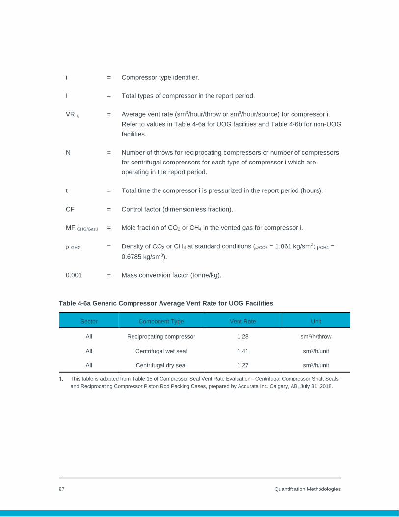
87 Quantifcation Methodologies
i = Compressor type identifier.
I = Total types of compressor in the report period.
VR i, = Average vent rate (sm3/hour/throw or sm3/hour/source) for compressor i.
Refer to values in Table 4-6a for UOG facilities and Table 4-6b for non-UOG
facilities.
N = Number of throws for reciprocating compressors or number of compressors
for centrifugal compressors for each type of compressor i which are
operating in the report period.
t = Total time the compressor i is pressurized in the report period (hours).
CF = Control factor (dimensionless fraction).
MF GHG/Gas,i = Mole fraction of CO2 or CH4 in the vented gas for compressor i.
GHG = Density of CO2 or CH4 at standard conditions (CO2 = 1.861 kg/sm3; CH4 =
0.6785 kg/sm3).
0.001 = Mass conversion factor (tonne/kg).
Table 4-6a Generic Compressor Average Vent Rate for UOG Facilities
Sector Component Type Vent Rate Unit
All Reciprocating compressor 1.28 sm3/h/throw
All Centrifugal wet seal 1.41 sm3/h/unit
All Centrifugal dry seal 1.27 sm3/h/unit
This table is adapted from Table 15 of Compressor Seal Vent Rate Evaluation - Centrifugal Compressor Shaft Seals
and Reciprocating Compressor Piston Rod Packing Cases, prepared by Accurata Inc. Calgary, AB, July 31, 2018.
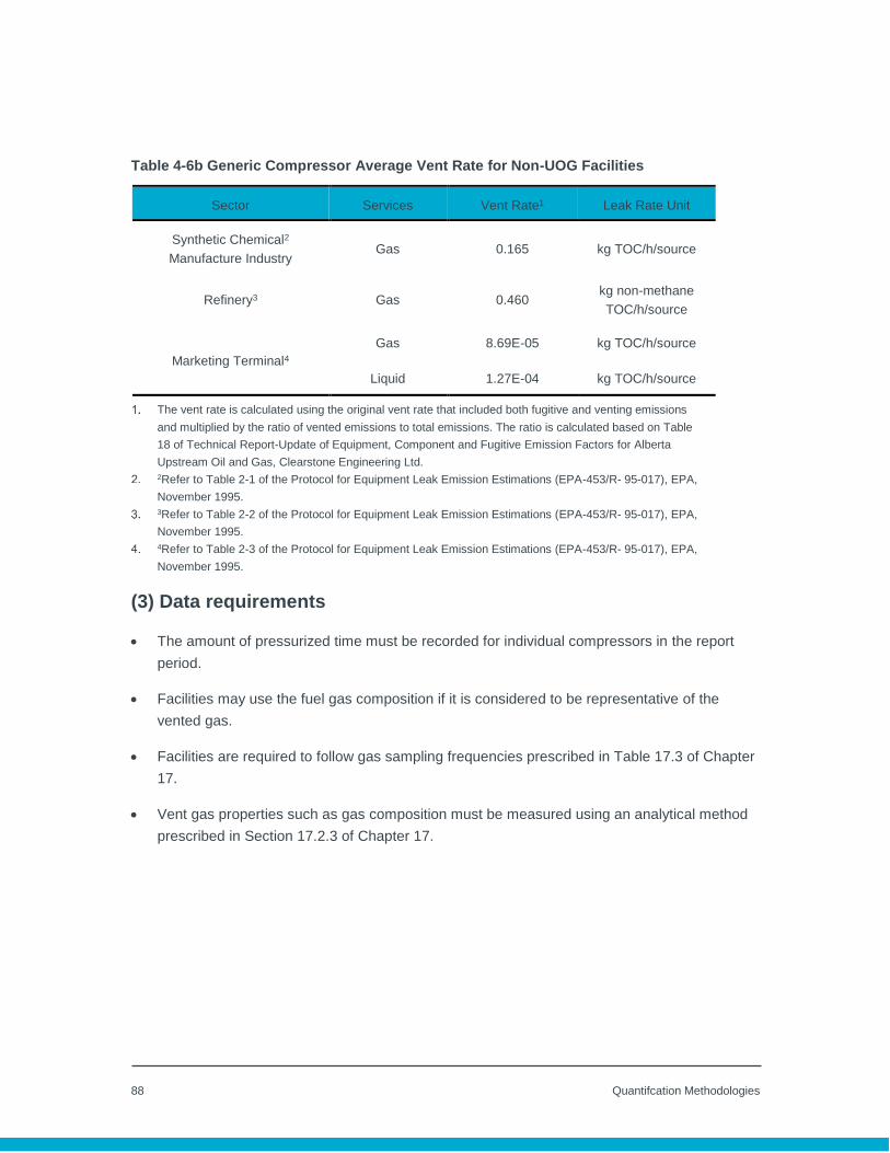
88 Quantifcation Methodologies
Table 4-6b Generic Compressor Average Vent Rate for Non-UOG Facilities
Sector Services Vent Rate1 Leak Rate Unit
Synthetic Chemical2
Manufacture Industry Gas 0.165 kg TOC/h/source
Refinery3 Gas 0.460 kg non-methane
TOC/h/source
Marketing Terminal4
Gas 8.69E-05 kg TOC/h/source
Liquid 1.27E-04 kg TOC/h/source
The vent rate is calculated using the original vent rate that included both fugitive and venting emissions
and multiplied by the ratio of vented emissions to total emissions. The ratio is calculated based on Table
18 of Technical Report-Update of Equipment, Component and Fugitive Emission Factors for Alberta
Upstream Oil and Gas, Clearstone Engineering Ltd.
2Refer to Table 2-1 of the Protocol for Equipment Leak Emission Estimations (EPA-453/R- 95-017), EPA,
November 1995.
3Refer to Table 2-2 of the Protocol for Equipment Leak Emission Estimations (EPA-453/R- 95-017), EPA,
November 1995.
4Refer to Table 2-3 of the Protocol for Equipment Leak Emission Estimations (EPA-453/R- 95-017), EPA,
November 1995.
(3) Data requirements
The amount of pressurized time must be recorded for individual compressors in the report
period.
Facilities may use the fuel gas composition if it is considered to be representative of the
vented gas.
Facilities are required to follow gas sampling frequencies prescribed in Table 17.3 of Chapter
17.
Vent gas properties such as gas composition must be measured using an analytical method
prescribed in Section 17.2.3 of Chapter 17.
89 Quantifcation Methodologies
4.9.3 Tiers 2 and 3-Manufacturer Vent Rate
(1) Introduction
This approach is applicable for compressors if the manufacturer vent rate is available for the
same make and model. Facilities that do not have manufacturer vent rates may use the tier 1
methodology.
(2) Equations
Calculate CH4 and CO2 emissions using Equation 4-14. The vent rate is provided by the
manufacturer based on the same or similar models and operating conditions. If the vent rate is
not available for a specific operating condition, use the highest emission rate available for the
manufacturer and model.
(3) Data requirements
Vent rates for the same or similar manufacturer, model and operating conditions provided by
the manufacturer should be used.
The vent rates should be converted to standard conditions.
Facilities may use the fuel gas composition if it is considered to be representative of the
vented gas.
The mole fraction is determined using the gas sampling frequencies prescribed in Table 17-3
of Chapter 17.
Vent gas properties such as gas composition must be measured using an analytical method
prescribed in Section 17.2.3 of Chapter 17.
4.9.4 Tier 4-Direct Measurement
(1) Introduction
As per AER Directive 060, facilities are required to measure compressor venting starting on
January 1, 2020. If a compressor piston-rod packing is replaced on one throw of a reciprocating
compressor seal after a test is completed, an average emission rate of 0.16 m3 vent gas per hour
per throw (adapted from AER Manual 15, December 2018) can be used until the next test is
completed.

90 Quantifcation Methodologies
This approach is applicable for compressors that are tied into an open-ended vent line and the
vent rate is measured periodically or continuously.
(2) Equations
The vent rate for reciprocating compressors should be calculated for each throw. The vent rate
for centrifugal compressors should be calculated for each seal. A facility may measure the total
vent rate at the vent line and determine the vent rate per throw or seal. For example, if a
compressor has four throws, but only three was operating during the test event, the facility may
calculate the vent rate per throw by dividing the total vent rate by three.
If the volumetric flow rate is measured such as using calibrated bag or volumetric meter, calculate
the GHG emissions using the Equation 4-14 using the following parameters.
VR i = Measured gas volumetric vent rate during operating time for compressor i
before the vent control equipment per throw (sm3/h/throw) for reciprocating
compressors and per unit for centrifugal compressors.
If the mass rate is measured such as using hi-flow sampling, calculate the GHG emissions using
the same equation as Equation 4-14. However, replace the volumetric rate (VRi) for compressor i
and GHG gas density (𝜌𝐺𝐻𝐺) by mass rate and replace the mole fraction by mass fraction.
MR i = Measured gas mass vent rate per throw (kg/h/throw) during operating time
for compressor i before the vent control equipment for reciprocating
compressors and per unit (kg/h/unit) for centrifugal compressors.
F GHG/THC = Mass fraction of CO2 or CH4 in the vented gas for compressor i.
(3) Data requirement
Refer to Section 4.1.2 for data requirements.
Vent rate should be measured annually at the compressor during normal operating
conditions.
Measure emissions using a high-flow sampler, calibrated bag, or appropriate meter.
The measurement locations must be representative of all potential vent paths. For instance,
for reciprocating compressors, the total vent rate should include all potential vented
emissions from the crank end to the head end. These include vented emissions from the

91 Quantifcation Methodologies
piston-rod packing vent and drain, distance piece vent and drain, and compressor crankcase
vent and drain if they are open to atmosphere.
For any compressor seal that emits vent gas, the seal must be measured at least every 9,000
hours that it is pressurized.
The volumetric vent rate must be converted to standard conditions.
If a continuous gas analyzer is available on the outlet gas stream, then the continuous gas
analyzer results must be used.
If a continuous gas analyzer is not present, the facility is required to follow gas sampling
frequencies prescribed in Table 17.3 of Chapter 17.
Vent gas properties such as gas composition must be measured using an analytical method
prescribed in Section 17.2.3 of Chapter 17.
Facilities may use the fuel gas composition if it is considered to be representative of the
vented gas.
4.10 Glycol Dehydrator Venting
4.10.1 Introduction
Glycol dehydrators are used to remove water from raw natural gas (wet gas) at gas batteries and
gas plants. While glycols easily absorb water, they have a tendency to absorb small amounts of
hydrocarbons (primarily benzene, hexane and heavier hydrocarbons, with some methane). These
impurities can be vented to atmosphere from the flash tank separator or the regenerator
overhead. If the dehydrator unit has vapor recovery, emissions must be adjusted by the amount
of emissions recovered, by applying a control factor as illustrated in Section 4.1.
4.10.2 Tiers 1, 2 and 3-GHG Based on Simulation Program
(1) Introduction
This method requires the use of simulation programs such as GRI-GLYCalc, Aspen HYSYS or
Prosim for quantifying venting emissions from dehydrators. For example, GRI-GLYCalc is
primarily intended for estimating benzene, toluene, ethyl benzene and xylene (BTEX) emitted by
a glycol dehydrator since significant amounts of this material may be preferentially absorbed by
the glycol and released off the flash tank and still column. However, the program can also provide

92 Quantifcation Methodologies
the total volume of vent gas and gas compositions, which provides sufficient information on
estimating the amount of methane emissions.
(2) Equations
Using the vent rate and gas composition calculated by the simulation program, Equation 4-10 can
be used to calculate the total GHG emissions using the following parameters:
VR = Simulated gas volumetric vent rate for glycol dehydrator i before the vent
control equipment (sm3/h).
t = Dehydrator running time (h) in the report period.
MF GHG/gas = CO2 or CH4 mole fraction based on the output of the simulation for glycol
dehydrator i (dimensionless).
Typical data inputs for various simulator programs are listed below:
Wet gas composition and flow rate.
Glycol circulation rate.
Temperature and pressure in the absorber column.
Type of glycol pump (electric or energy exchange).
Operating pressure of the flash tank (if one is used) and amount of flash gas used by the
process (if at all).
Type of glycol (TEG or DEG).
Stripping gas (if used).
Temperature and pressure of flash tank (if present).
(3) Data requirements
Facilities are required to follow gas sampling frequencies for wet gas analysis prescribed in
Table 17-3 of Chapter 17.
Wet gas flow rate and circulation rate should be metered continuously and documented for a
glycol dehydrator.
93 Quantifcation Methodologies
At glycol dehydrator sites, if the dry gas water content is routinely measured, use the
measured data. Otherwise, design values for dry gas water content or the number of
equilibrium stages in the absorber may be used.
4.11 Glycol Refrigeration Venting
(1) Introduction
Dehydration and refrigeration in the oil and gas industry is used to lower the temperature at which
hydrates form or to remove water from natural gas streams, or both. It is more common to lower
the hydrate temperature by injecting glycol in the gas after separation of free water.
The associated emissions released during the regeneration of glycol are similar to glycol
dehydration and uses the same methodology.
(2) Equations
Refer to Section 4.10 for equations.
(3) Data requirements
Refer to Section 4.10 for data requirements.
4.12 Acid Gas Removal (AGR)/Sulphur Recovery Units Venting
4.12.1 Introduction
Sour gas, which is natural gas with high concentrations of acid gas species (H2S and CO2), must
be treated to reduce the acid gases to a concentration that meets pipeline transportation criteria.
Acid Gas Removal (AGR) units remove H2S and CO2 by contacting the sour gas with a liquid
solution (typically amines). There are other acid gas removal technologies besides amine units,
including the Morphysorb® process, Kvaerner Membrane technology, and the Molecular Gate®
process, the latter of which involves the use of molecular sieves. These technologies are reported
to reduce CH4 emissions too.
Sour gas processing or sulfur recovery units (SRU) can directly vent the CO2 removed from the
sour gas stream to the atmosphere or capture the CO2 for other uses, such as enhanced oil
recovery. These emissions are considered to be formation CO2 and should be reported under
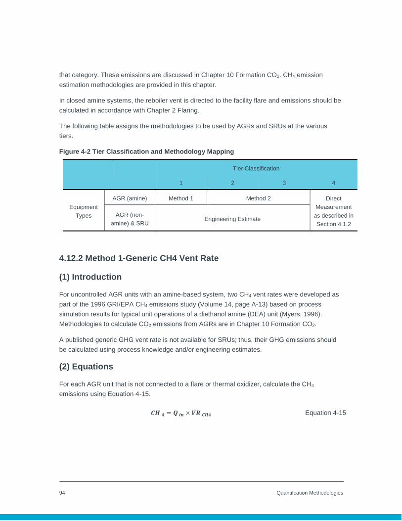
94 Quantifcation Methodologies
that category. These emissions are discussed in Chapter 10 Formation CO2. CH4 emission
estimation methodologies are provided in this chapter.
In closed amine systems, the reboiler vent is directed to the facility flare and emissions should be
calculated in accordance with Chapter 2 Flaring.
The following table assigns the methodologies to be used by AGRs and SRUs at the various
tiers.
Figure 4-2 Tier Classification and Methodology Mapping
Tier Classification
1 2 3 4
Equipment
Types
AGR (amine) Method 1 Method 2 Direct
Measurement
as described in
Section 4.1.2
AGR (non-
amine) & SRU Engineering Estimate
4.12.2 Method 1-Generic CH4 Vent Rate
(1) Introduction
For uncontrolled AGR units with an amine-based system, two CH4 vent rates were developed as
part of the 1996 GRI/EPA CH4 emissions study (Volume 14, page A-13) based on process
simulation results for typical unit operations of a diethanol amine (DEA) unit (Myers, 1996).
Methodologies to calculate CO2 emissions from AGRs are in Chapter 10 Formation CO2.
A published generic GHG vent rate is not available for SRUs; thus, their GHG emissions should
be calculated using process knowledge and/or engineering estimates.
(2) Equations
For each AGR unit that is not connected to a flare or thermal oxidizer, calculate the CH4
emissions using Equation 4-15.
𝑪𝑯 𝟒 = 𝑸 𝒊𝒏 × 𝑽𝑹 𝑪𝑯𝟒 Equation 4-15

95 Quantifcation Methodologies
Where:
CH 4,p = CH4 mass emissions (tonnes) from the AGR unit venting in the report
period.
Q in,p = Metered total volume natural gas flow into the AGR unit converted to
standard condition per Appendix C (106 scf or 106m3) in the report period.
VR CH4 = Methane vent rate for the AGR unit in Table 4-7 (tonnes/106scf or
tonnes/106 m3).
Table 4-7 Uncontrolled AGR CH4 Vent Rate
Source Methane Vent Rate3, Original
Units
Methane Vent Rate4, Converted to
Tonnes Basis
AGR vent
965 scf/106
scf treated gas 0.0185 tonnes/106
scf treated gas
0.654 tonnes/106
m3
treated gas
This table is adapted from Table 5-5 of Compendium of Greenhouse Gas Emissions Methodologies for the
Oil and Natural Gas Industry, American Petroleum Institute (API), August 2009.
(3) Data requirements
The AGR throughputs may be metered or quantified based on accounting procedures.
4.12.3 Method 2-Vent Rate Using Simulation
(1) Introduction
API’s AMINECalc is designed to estimate hydrocarbon emissions from amine based sour gas and
natural gas liquid (NGL) sweetening units. The amine system normally consists of a contactor,
flash drum and regenerator. The CH4 and CO2 emissions can be estimated from total
hydrocarbon emissions
3 Myers, D.B. Methane Emissions from the Natural Gas Industry, Volume 14: Glycol Dehydrators, Final Report, GRI-94/0257.31 and EPA- 600/R-96-080n, Gas Research Institute and U.S. Environmental Protection Agency, June 1996. Based on a DEA unit. 4 CH4 emission factors converted from scf are based on 60°F and 14.7 psia.
96 Quantifcation Methodologies
(2) Equations
Calculate CH4 or CO2 emissions using Equation 4-10 using the outputs from AMINECalc
including the vent rate and gas compositions.
(3) Data requirements
The AGR throughputs may be metered or quantified based on accounting procedures.
4.13 Hydrocarbon Liquid Loading/Unloading Venting
4.13.1 Introduction
The vapors from cargo tanks can be displaced directly into the atmosphere when petroleum liquid
is loaded into those vessels in the absence of any specific controls. If a separation system is
installed to control loading losses from the tank vehicles, or to balance or exchange vapors
between the tanks and tank vehicles, the loading/unloading losses are greatly reduced. Loading
of petroleum products into railcars or tank-trucks occurs at UOG, oil storage tank farms, upgrader
and refining facilities.
CH4 or CO2 emissions in most petroleum products including stabilized (weathered) crude are
negligible. Unstabilized crude oil contains sufficient dissolved gas hydrocarbons (mainly C1, C2,
C3 and C4) that may be released from the oil at separator conditions. Therefore, evaporative
emissions associated with loading/unloading is only for unstabilized crude.
4.13.2 Tiers 1, 2 and 3-Algorithm
Method 1: Loading Emissions from Low Vapor Pressure (LVP)
Loading
(1) Introduction
Rail tank cars and tank trucks transport low vapor pressure (LVP) products such as crude oil,
condensate and pentanes-plus. Emissions due to the displacement of tank vapors (i.e.
evaporated product) can occur during the loading of these carriers. The amount of emissions
depends on the vapor pressure of the liquid product, recent loading history and method of
loading.

97 Quantifcation Methodologies
(2) Equations
This approach calculates the total vapor emissions and then uses GHG composition in the vapor
to calculate specific GHG emissions. Calculate GHG loading emissions for all products loaded in
the report period using Equation 4-16.
𝑮𝑯𝑮 = ∑𝟎. 𝟏𝟐𝟎 × 𝑺𝑭 𝒋 × 𝑷 𝑻𝒓𝒖𝒆,𝒋 × 𝑸 𝒋 × 𝑴𝑾 𝒗𝒂𝒑𝒐𝒓 × 𝑭 𝑮𝑯𝑮,𝒗𝒂𝒑𝒐𝒓
(𝑻 𝒋 + 𝟐𝟕𝟑. 𝟏𝟓)
𝒏
𝒋=𝟏
× 𝟎. 𝟎𝟎𝟏 × (𝟏 − 𝑪𝑭)
Equation 4-16
Where:
GHG = CH4 or CO2 mass emissions (tonnes) from loading loss of product j in the
report period.
j = Product type.
n = Types of product loaded.
0.120 = Constant (k kmol/kpa m3).
Q j = Volume of the LVP product loaded in the report period (m3).
MW vapor = Molecular weight of vapor (kg/kmol).
P true,j = True vapor pressure of the loaded LVP product j (kPa) at bulk liquid temp
(Tj). Determined by multiplying the vapor pressure (psi) from Equation 4-
16a or Equation 4-16b by 6.8948 to convert psi to kpa.
SF j = Saturation factor for LVP product j from Table 4-8 to account for the effects
of the method of loading (dimensionless).
CF = Average emission control factor (dimensionless) for the control system
installed, CF is 0 in absence of control system.
T j = Bulk temperature of the LVP product j loaded (◦C).
F GHG ,vapor = Mass fraction of CH4 or CO2 in vapor evaporated from product j loading.

98 Quantifcation Methodologies
For crude oils with Reid Vapor Pressures (RVP) of 2 to 15 pounds per square inch (psi), use
Equation 4-16a to convert to a true vapor pressure, and then convert the true vapor pressure
from psi to kpa for Equation 4-16.
𝑷 𝒕𝒓𝒖𝒆,𝒋 = 𝐞𝐱𝐩{[𝟐𝟕𝟗𝟗
(𝑻 + 𝟒𝟓𝟗. 𝟔)− 𝟐. 𝟐𝟐𝟕] 𝐥𝐨𝐠𝟏𝟎(𝑹𝑽𝑷) −
𝟕𝟐𝟔𝟏
(𝑻 + 𝟒𝟓𝟗. 𝟔)+ 𝟏𝟐. 𝟖𝟐} Equation 4-16a
Where:
P true,j = True vapor pressure of loaded LVP product j, in pounds per square inch
absolute (psia).
T = Bulk temperature of the loaded LVP product j, in degree Fahrenheit (◦F).
RVP = Reid Vapor Pressure of liquid j, in psi; sampled for the liquid j or taken from
Table 4-9.
For refined products having a RVP value of 1 to 20 psi, use Equation 4-16b to calculate the true
vapor pressure from RVP, and then convert true vapor pressure in psi to kpa for Equation 4-16.
𝑃 𝑡𝑟𝑢𝑒,𝑗 = exp{[0.7553 − (413.0
𝑇 + 459.6)] × (𝑆)0.5 × log10(𝑅𝑉𝑃)
− [1.854 − (1042
𝑇 + 459.6)] × (𝑆)0.5
+ [(2416
𝑇 + 459.6) − 2.013] log10(𝑅𝑉𝑃) −
8742
(𝑇 + 459.6)+ 15.64}
Equation 4-16b
Where:
Ptrue,j = True vapor pressure of loaded LVP product j, in pounds per square inch
absolute (psia).
RVP = Reid Vapor Pressure of liquid j, in psi; sampled for the liquid j or taken from
Table 4-9.
S = Slope of the ASTM distillation curve at 10 percent evaporated, in degree
Fahrenheit (°F/vol%), refer to Table 4-10.
T = Bulk temperature of the loaded LVP product j, in degree Fahrenheit (◦F).

99 Quantifcation Methodologies
RVP = Reid Vapor Pressure of liquid j, in psi; sampled for the liquid j or taken from
Table 4-9.
Table 4-8: Saturation Factors for Petroleum Liquid Loading Losses
Cargo Carrier Mode of Operation Saturation Factor
(Dimensionless)
Tank trucks and rail tank
cars
Submerged loading of a clean cargo tank 0.50
Submerged loading: dedicated normal service 0.60
Submerged loading: dedicated vapor balance service 1.00
Splash loading of a clean cargo tank 1.45
Splash loading: dedicated normal service 1.45
Splash loading: dedicated vapor balance service 1.00
Saturation [S] Factors for Calculation of Petroleum Liquid Loading Losses, USEPA AP-42, 5th Edition, Volume 1,
Chapter 5: Petroleum Industry.
Table 4-9: Liquid Product Properties for Loading and Unloading Emission Estimates
Liquid Product Oil Specific
Gravity
Reid Vapor Pressure
(RVP)
Vapor Molecular
Weight
(kPa) (psi) (kg/kmol)
Condensate 0.715 76.6 11.11 28.2
Light/Medium Crude Oil 0.8315 54.8 7.95 44.2
Heavy Crude Oil 0.9153 40.5 5.87 19.9
Thermal Crude Oil 0.9153 40.5 5.87 30.6
Cold Bitumen 0.9182 39.7 5.76 23.3
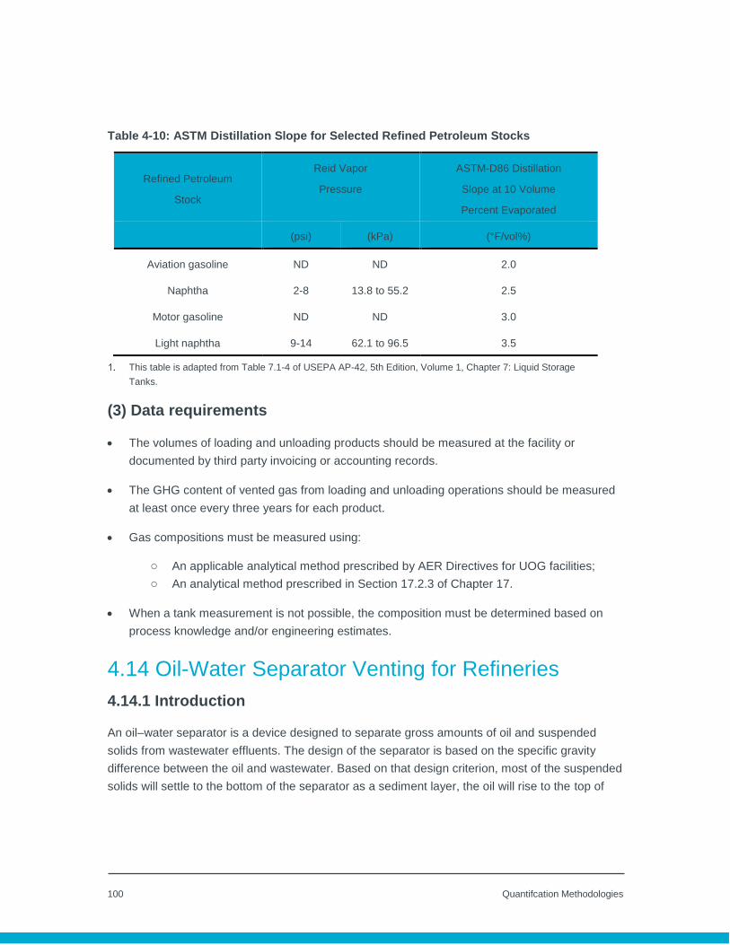
100 Quantifcation Methodologies
Table 4-10: ASTM Distillation Slope for Selected Refined Petroleum Stocks
Refined Petroleum
Stock
Reid Vapor
Pressure
ASTM-D86 Distillation
Slope at 10 Volume
Percent Evaporated
(psi) (kPa) (°F/vol%)
Aviation gasoline ND ND 2.0
Naphtha 2-8 13.8 to 55.2 2.5
Motor gasoline ND ND 3.0
Light naphtha 9-14 62.1 to 96.5 3.5
This table is adapted from Table 7.1-4 of USEPA AP-42, 5th Edition, Volume 1, Chapter 7: Liquid Storage
Tanks.
(3) Data requirements
The volumes of loading and unloading products should be measured at the facility or
documented by third party invoicing or accounting records.
The GHG content of vented gas from loading and unloading operations should be measured
at least once every three years for each product.
Gas compositions must be measured using:
o An applicable analytical method prescribed by AER Directives for UOG facilities;
o An analytical method prescribed in Section 17.2.3 of Chapter 17.
When a tank measurement is not possible, the composition must be determined based on
process knowledge and/or engineering estimates.
4.14 Oil-Water Separator Venting for Refineries
4.14.1 Introduction
An oil–water separator is a device designed to separate gross amounts of oil and suspended
solids from wastewater effluents. The design of the separator is based on the specific gravity
difference between the oil and wastewater. Based on that design criterion, most of the suspended
solids will settle to the bottom of the separator as a sediment layer, the oil will rise to the top of
101 Quantifcation Methodologies
the separator, and the wastewater will be contained in the middle layer. Air is introduced to
increase the floatation of oil in order to enhance oil removal.
4.14.2 Tiers 1, 2 and 3-Generic Vent Rate
(1) Introduction
The generic vent rate is based on non-methane hydrocarbon vent rate (NMHC) from different
types of refinery separators. Separators are also used in petrochemical plants, chemical plants,
natural gas processing plants and other industrial oil-water separators, which are not covered in
this section. Facilities other than refineries should calculate CH4 emissions from oil-water
separators using process knowledge and engineering estimates.
(2) Equations
Calculate CH4 emissions from oil-water separators at refineries using Equation 4-17.
𝐶𝐻 4 = 𝑉𝑅 𝑠𝑒𝑝 × 𝑄 𝑤𝑎𝑡𝑒𝑟 × 𝐹 𝐶𝐻4/𝑁𝑀𝐻𝐶 × (1 − 𝐶𝐹) × 0.001 Equation 4-17
Where:
CH 4 = CH4 mass emissions (tonnes) from oil water separator in the report
period.
Q water = Volume of the wastewater treated in the oil water separator in the report
period (m3).
VR sep = NMHC (non-methane hydrocarbon) emission factor (kg/m3) from Table 4-
11.
CF = Control factor of the oil water separator emission control (dimensionless).
F CH4/NMHC = Mass fraction of CH4 to NMHC. Use either a default factor of 0.6 or
species specific conversion factors determined by analysis or estimation.
0.001 = Convert factor from kg to tonnes.

102 Quantifcation Methodologies
Table 4-11: Vent Rate for Oil/Water Separators
Separator Type Vent Rate5
(kg NMHC/m3 wastewater treatment)
Gravity Type-uncovered 1.11 × 10⁻¹
Gravity Type-covered 3.30 × 10⁻³
Dissolved air flotation type or induced air flotation type -
uncovered6 4.00 × 10⁻³
Dissolved air flotation type or induced air flotation type -
covered6 1.20 × 10⁻⁴
This table is adapted from Table 11-3 of Canada’s Proposed Greenhouse Gas Quantification Requirements, ECCC
Canada, September 2018.
(3) Data requirements
Wastewater volume treated in the oil-water separator is documented.
The mass fraction of methane to NMHC should be measured once per year at minimum
where the default is not used. It should also be measured whenever operating conditions, oil
content in water, or oil properties change.
Measurements must be conducted using:
o An applicable analytical method prescribed by AER Directives for UOG facilities;
o An applicable method published by a consensus-based standards organization; or
o An analytical method prescribed in Section 17.2.3 of Chapter 17.
When a measurement is not possible, the composition must be determined based on process
knowledge and/or engineering estimates.
5 Vent rates do not include ethane 6 Vent rates for these types of separators apply where they are installed as secondary treatment systems

103 Quantifcation Methodologies
4.15 Produced Water Tank Venting
4.15.1 Introduction
Produced water is water found in the same formation as oil and gas. When the oil and gas flow to
the surface, the produced water is brought to the surface with the hydrocarbons. Produced water
can also be water that was previously injected into those formations through activities designed to
increase oil production from the formations such as water flooding or steam flooding operations.
In some situations additional water from other formations adjacent to the hydrocarbon-bearing
layers may become part of the produced water that comes to the surface. Flowback water
following hydraulic fracturing is often managed in a similar manner as produced water and is
often consider as part of the produced water flow stream. Produced water contains some of the
chemical characteristics of the formation from which it was produced and associated
hydrocarbons. Produced water is also commonly referred to as saltwater.
Common produced water tanks are atmospheric storage tanks that are located at saltwater
disposal sites that store produced water in preparation for disposal. Produced water can be
stored in tanks located at oil and gas exploration and production activities, to receive liquids from
a separator.
Produced water tank emissions occur in a manner similar to crude oil storage tank flashing
losses. Methane emissions from produced water tanks are lower than crude tank flashing losses
because CH4 has a stronger affinity for hydrocarbon oil than it does for water. Thus, less CH4 is
dissolved in the water phase. Varying amounts of CH4 are emitted from the produced water
depending on the temperature and pressure in the produced water tanks.
4.15.2 Tiers 1, 2, and 3–Generic Vent Rate
(1) Introduction
CH4 emissions are estimated by using the vent rate from produced water tanks, produced water
volume and vapor control on the produced water tank by using Equation 4-18.
(2) Equations
𝐶𝐻 4 = 𝑉 𝑃,𝑤𝑎𝑡𝑒𝑟 × 𝑉𝑅 𝐶𝐻4 × (1 − 𝐶𝐹) Equation 4-18

104 Quantifcation Methodologies
Where:
CH4 = CH4 mass emissions (tonnes) from produced water tank venting in the
report period.
V p,water = Volume of produced water (1000 m3).
CF = Control factor of the produced water tank emission control
(dimensionless).
VR CH4 = CH4 vent rate related to separator pressure and salt content of
produced water in Table 4-12a and 4-12b.
Table 4-12a: Produced Salt Water Tank Methane Flashing Vent Rate1
Separator Pressure (psi) Produced Water Salt Content Water Tank Vent Rate (VR CH4)
tonnes CH4 /1000 m3 produced water
50 20% 0.009185
250 20% 0.06200
250 10% 0.09414
250 2% 0.11137
250 Average of 10.7% 1 0.08917
1000 20% 0.22273
1000 10% 0.33697
1000 2% 0.39896
1000 Average of 10.7% 1 0.31955
This table is adapted from Table 5-10 of Compendium of Greenhouse Gas Emissions Methodologies for the
Oil and Natural Gas Industry, American Petroleum Institute (API), August 2009. Average of emissions factors
for 20%, 10% and 2% produced water salt content.
Average of vent rates at 20%, 10% and 2% salt.

105 Quantifcation Methodologies
Table 4-12b: Methane Vent Rates from Produced Water from Shallow Gas Wells
Source Information CH4 Water Tank Vent Rate
Shallow gas well
(76 psi or less, 50°C)
0.036 tonnes CH4/1000 m3
produced water
This table is adapted from Table 5-11 of Compendium of Greenhouse Gas Emissions Methodologies
for the Oil and Natural Gas Industry, American Petroleum Institute (API), August 2009.
(3) Data requirements
Produced water volume and salt content should be measured or calculated based on
engineering estimates.
4.16 Non-Routine Venting-Well Tests, Completion, and Workovers
4.16.1 Introduction
Non-routine well tests, completion, and workovers are planned events that result in venting
emissions.
4.16.2 Tiers 1, 2 and 3
(1) Introduction
Hydrocarbon venting from well tests, completions and workovers should be quantified as required
by AER Directive 040: Pressure and Deliverability Testing Oil and Gas Wells and Directive 059:
Well Drilling and Completion Data Filing Requirements.
(2) Equations
For each blowdown event, calculate CH4 or CO2 emissions and sum the CH4 or CO2 emissions
from blowdown events to calculate total emissions in the report period using Equation 4-19.
𝑮𝑯𝑮 = ∑ 𝑸 𝒗 × 𝑴𝑭 𝑮𝑯𝑮 × 𝝆 𝑮𝑯𝑮 × 𝟎. 𝟎𝟎𝟏
𝒏
𝒊=𝟏
Equation 4-19

106 Quantifcation Methodologies
Where:
GHG = CH4 or CO2 mass emissions (tonnes) from well tests, completion
and workovers events in the report period.
i = Vent event identifier.
n = Number of events in the report period.
Q v = Total vented gas volume (m3) during a well test, completion or
workover event.
MF GHG = Mole fraction of CO2 or CH4 in vented gas.
GHG = Density of CO2 or CH4 at standard conditions (CO2 = 1.861
kg/sm3; CH4 = 0.6785 kg/sm3).
0.001 = Mass conversion factor (tonne/kg).
(3) Data requirements
The vented gas volume during the event must be quantified according to AER Directive 040
for minimum standards for performing well tests, and AER Directive 059 requirements for
drilling, completion, reconditioning, or well abandonment.
The composition of the vented gas should be measured before a planned event. Gas
compositions must be measured using:
o An applicable analytical method prescribed by AER Directives for UOG facilities;
o An analytical method prescribed in Section 17.2.3 of Chapter 17.
When a measurement is not possible, the composition must be determined based on process
knowledge and/or engineering estimates.
4.17 Non-Routine Venting-Process System Blowdown
4.17.1 Introduction
GHG emissions may be vented to atmosphere during blowdown events required for planned or
emergency depressurization (e.g., evacuating process systems or emergency shutdown events).

107 Quantifcation Methodologies
4.17.2 Tiers 1, 2 and 3-Algorithm
(1) Introduction
This quantification method requires an estimation of the volume of the process system that is
evacuated and a measurement or estimation of the composition of the evacuated gas.
(2) Equations
For blowdown emissions, calculate CH4 or CO2 emissions for each event and sum the CH4 or
CO2 emissions from blowdown events to calculate total emissions in the report period.
When the operating conditions represent ideal gas conditions (i.e. gas is not expected to
condense due to high pressure and low temperature), use Equation 4-5a to calculate the
blowdown emissions.
When the operating conditions represent non-ideal gas conditions (i.e. gas is expected to
condense due to high pressure and low temperature), use Equation 4-5b to calculate the
blowdown emissions.
(3) Data requirements
Refer to Section 4.5 for ideal gas or non-ideal gas data requirements.
4.18 Non-Routine Venting-Gas Well Liquids Unloading
4.18.1 Introduction
Gas well liquid unloading is a procedure, implemented periodically, where liquids that have
accumulated in a gas well are removed to surface equipment. The conventional method of liquids
unloading is to use the natural reservoir pressure to lift the liquids accumulated in the tubing to
the surface. When reservoir pressure declines, plunger lifts can be used to assist with liquids
unloading. In both situations, gas will be vented to the atmosphere. The following equation is
used for calculating venting emissions for both natural reservoir pressure and plunger lift
unloading procedures.

108 Quantifcation Methodologies
4.18.2 Tiers 1, 2, and 3-Algorithm
(1) Introduction
The algorithm method estimates the vented gas volume based on the physical dimensions of the
casing or plunger lift used for a liquids unloading operation.
(2) Equations
For each liquids unloading venting source, calculate CH4 or CO2 emissions for each well
unloading event and add the total emissions for all unloading events in the report period using
Equation 4-20.
𝑮𝑯𝑮 = ∑ [(𝟕. 𝟖𝟓𝟒 × 𝟏𝟎−𝟓 × 𝑫𝟐 × 𝑾𝑫 × [
𝑺𝑷
𝟏𝟎𝟏. 𝟑𝟐𝟓])
+𝑸 𝒔𝒇𝒓 × 𝒕 𝒐𝒑𝒆𝒏
]
𝒊
𝒏
𝒊=𝟏
× 𝑴𝑭 𝑮𝑯𝑮/𝑮𝒂𝒔
× 𝝆 𝑮𝑯𝑮 × 𝟎. 𝟎𝟎𝟏
Equation 4-20
Where:
GHG = CH4 or CO2 mass emissions (tonnes) from gas well liquid unloading
venting in the report period.
i = Gas well liquid unloading event identifier.
n = Number of gas well liquid unloading events in report period.
7.854×10-5 = (π/4)/(10,000).
D = Production casing diameter of the well (cm).
WD = Well depth (m).
SP = Well shut-in pressure at well head pressure gauge (kPag).
Q sfr = Maximum monthly sales flow rate of the gas well observed over the
report period from production records metered at or converted to
standard conditions (Sm3/h).

109 Quantifcation Methodologies
t open = Hours that the well was left open to the atmosphere during unloading.
101.325 = Standard absolute pressure (kPaa).
MF GHG/Gas = Mole fraction of CO2 or CH4 in vented gas.
GHG = Density of CO2 or CH4 at standard conditions (CO2 = 1.861 kg/sm3;
CH4 = 0.6785 kg/sm3)
0.001 = Mass conversion factor (tonne/ kg).
(3) Data requirements
Document the length of time (hours) that the well is open to atmosphere and well gauge
pressure for each event.
The composition of vented gas should be measured before a planned event or determined
based on process knowledge and/or engineering estimates.
Gas compositions must be measured using:
o An applicable analytical method prescribed by AER Directives for UOG facilities;
o An analytical method prescribed in Section 17.2.3 of Chapter 17.
4.18.3 Tier 4-Direct Measurement
(1) Introduction
This method is for wells that have a flow meter installed on the vent line used to vent gas from the
well (e.g. on the vent line off the wellhead separator or atmospheric storage tank).
(2) Equations
Calculate emission from well venting for liquids unloading using Equation 4-21.
𝑮𝑯𝑮 = ∑[𝑽𝑹 𝒊 × 𝒕 𝒕𝒐𝒕𝒂𝒍,𝒊 × (𝟏 − 𝑪𝑭)]
𝒏
𝒊=𝟏
× [𝑷
𝟏𝟎𝟏. 𝟑𝟐𝟓] × 𝑴𝑭𝑮 𝑯𝑮/𝑮𝒂𝒔
× 𝝆 𝑮𝑯𝑮 × 𝟎. 𝟎𝟎𝟏
Equation 4-21

110 Quantifcation Methodologies
Where:
GHG = CH4 or CO2 mass emissions (tonnes) from gas well liquid unloading
venting in the report period.
i = Well identifier.
n = Number of wells with the same tubing diameter and producing
horizon/formation combination as the measured well.
VR i = The well vent average flow rate of the measured well i venting for
the duration of the liquids unloading event under actual conditions
(m3/hour).
t total,i = Cumulative amount of time in hours of venting from the well i
(hour).
P = Absolute pressure at the actual conditions that the flow rate is
measured at (kPaa).
CF = Control factor (dimensionless fraction).
101.325 = Standard absolute pressure (kPaa).
MF GHG/Gas = Mole fraction of CO2 or CH4 in vented gas.
GHG = Density of CO2 or CH4 at standard conditions (CO2 = 1.861 kg/sm3;
CH4 = 0.6785 kg/sm3).
0.001 = Mass conversion factor (tonne/ kg).
(3) Data requirements
Refer to Section 4.1.2 for data requirements.
A well vent flow rate measurement should be conducted in accordance with Chapter 17.
Determine the well vent average flow rate as specified in the following:
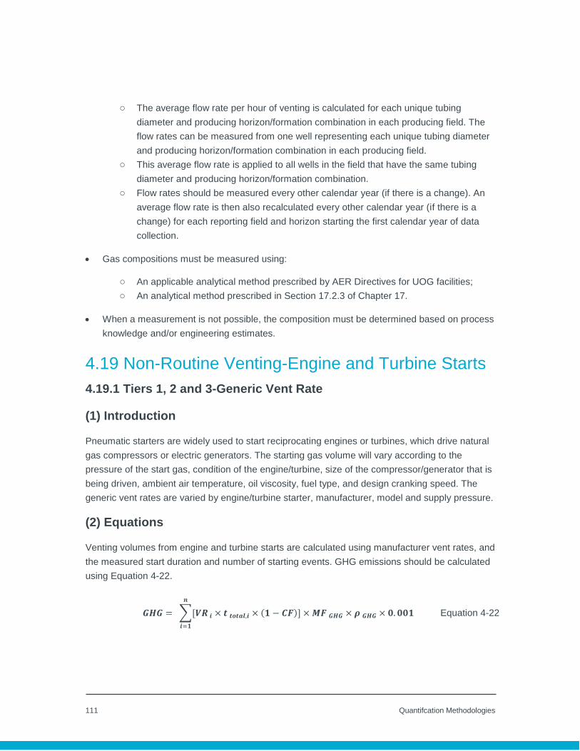
111 Quantifcation Methodologies
o The average flow rate per hour of venting is calculated for each unique tubing
diameter and producing horizon/formation combination in each producing field. The
flow rates can be measured from one well representing each unique tubing diameter
and producing horizon/formation combination in each producing field.
o This average flow rate is applied to all wells in the field that have the same tubing
diameter and producing horizon/formation combination.
o Flow rates should be measured every other calendar year (if there is a change). An
average flow rate is then also recalculated every other calendar year (if there is a
change) for each reporting field and horizon starting the first calendar year of data
collection.
Gas compositions must be measured using:
o An applicable analytical method prescribed by AER Directives for UOG facilities;
o An analytical method prescribed in Section 17.2.3 of Chapter 17.
When a measurement is not possible, the composition must be determined based on process
knowledge and/or engineering estimates.
4.19 Non-Routine Venting-Engine and Turbine Starts
4.19.1 Tiers 1, 2 and 3-Generic Vent Rate
(1) Introduction
Pneumatic starters are widely used to start reciprocating engines or turbines, which drive natural
gas compressors or electric generators. The starting gas volume will vary according to the
pressure of the start gas, condition of the engine/turbine, size of the compressor/generator that is
being driven, ambient air temperature, oil viscosity, fuel type, and design cranking speed. The
generic vent rates are varied by engine/turbine starter, manufacturer, model and supply pressure.
(2) Equations
Venting volumes from engine and turbine starts are calculated using manufacturer vent rates, and
the measured start duration and number of starting events. GHG emissions should be calculated
using Equation 4-22.
𝑮𝑯𝑮 = ∑[𝑽𝑹 𝒊 × 𝒕 𝒕𝒐𝒕𝒂𝒍,𝒊 × (𝟏 − 𝑪𝑭)]
𝒏
𝒊=𝟏
× 𝑴𝑭 𝑮𝑯𝑮 × 𝝆 𝑮𝑯𝑮 × 𝟎. 𝟎𝟎𝟏 Equation 4-22

112 Quantifcation Methodologies
Where:
GHG = CH4 or CO2 mass emissions from engine or turbine start events
(tonnes) in the report period.
VR = Manufacturer vent rate for the engine or turbine stated in Table 4-13
(m3 NG/hour).
i = Engine or turbine identifier.
n = Number of engines or turbines.
t total,j = Total time for engine or turbine i starts in the report period calculated
using Equation 4-22a (hr).
CF = Control factor (dimensionless fraction).
MF GHG = Mole fraction of CO2 or CH4 in vented gas.
GHG = Density of CO2 or CH4 at standard conditions (CO2 = 1.861 kg/sm3;
CH4 = 0.6785 kg/sm3).
0.001 = Conversion factor from kg to tonne.
𝒕 𝒕𝒐𝒕𝒂𝒍,𝒋 = 𝒕 𝒖𝒏,𝒔𝒕𝒂𝒓𝒕 × 𝑵 𝒖𝒏.𝒋 + 𝒕 𝒔,𝒔𝒕𝒂𝒓𝒕 × 𝑵 𝒔,𝒋 Equation 4-22a
Where:
t total,j = Total start duration (hr) for engine or turbine j in the report period.
t un,start = Average duration per unsuccessful engine or turbine start (hr/start).
N un.j = Number of unsuccessful starts.
T s,start = Average duration per successful engine or turbine start (hr/start).
N un.j = Number of successful starts.
113 Quantifcation Methodologies
(3) Data requirements
The successful and unsuccessful starts, and their durations should be documented.
Facilities are required to follow gas sampling frequencies prescribed in Table 17.3 of Chapter
17.
Fuel properties such as gas composition must be measured using an analytical method
prescribed in Section 17.2.3 of Chapter 17.
When vendor flow rates are available, which typically assumes compressed air as the
working medium, air consumption rates must be multiplied by 1.29 for equivalent natural gas
consumption rates (with ±25% typical uncertainty).

114 Quantifcation Methodologies
Table 4-13: Pneumatic Starter Natural Gas Consumption Rate by Engine/Turbine
Engine/Turbine Pneumatic Starter
Manufacturer Model Manufacturer Model Supply
Pressure
(kPag)
Max. Natural Gas
Consumption Rate1
(m3/min) (m3/hour)
Turbines
Allison 501-KB
501-KC
Ingersoll Rand TS799B 1,034 80 4,822
Tech Development 56K (Low Pressure) 345 33 1,954
56K (Standard Pressure) 621 55 3,288
570 Ingersoll Rand TS799G 621 51 3,068
Dresser Clark DC990 Tech Development 56B (Low Pressure) 345 36 1,954
56B (Standard Pressure) 1,034 86 5,172
Dresser Rand DR990
DJ50
Tech Development 56B (Low Pressure) 345 36 1,954
56B (Standard Pressure) 1,034 86 5,172
Garrett IE831 Ingersoll Rand TS999G 621 47 2,849

115 Quantifcation Methodologies
Engine/Turbine Pneumatic Starter
Manufacturer Model Manufacturer Model Supply
Pressure
(kPag)
Max. Natural Gas
Consumption Rate1
(m3/min) (m3/hour)
General Electric LM500
LM1000
LM1600
LM2500
LM5000
LM6000
Tech Development 56G (Low Pressure) 345 33 1,954
56G (Standard Pressure) 1,034 86 5,172
Pratt & Whitney GG3/F13
GG4/G14
Ingersoll Rand TS799B 1,034 80 4,822
GG3
GG4
FT4
FT8
Tech Development 56A (Low Pressure) 345 33 1,954
56A (Standard Pressure) 1,034 86 5,172
Rolls Royce AVON
SPEY
Tech Development 56A (Low Pressure) 345 33 1,954
56A (Standard Pressure) 1,034 86 5,172
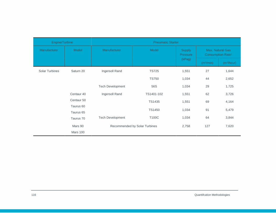
116 Quantifcation Methodologies
Engine/Turbine Pneumatic Starter
Manufacturer Model Manufacturer Model Supply
Pressure
(kPag)
Max. Natural Gas
Consumption Rate1
(m3/min) (m3/hour)
Solar Turbines Saturn 20 Ingersoll Rand TS725 1,551 27 1,644
TS750 1,034 44 2,652
Tech Development 56S 1,034 29 1,725
Centaur 40
Centaur 50
Taurus 60
Taurus 65
Taurus 70
Ingersoll Rand TS1401-102 1,551 62 3,726
TS1435 1,551 69 4,164
TS1450 1,034 91 5,479
Tech Development T100C 1,034 64 3,844
Mars 90
Mars 100
Recommended by Solar Turbines 2,758 127 7,620
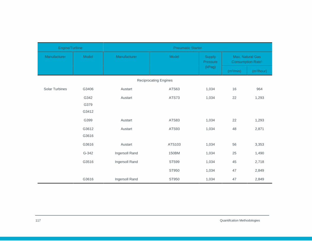
117 Quantifcation Methodologies
Engine/Turbine Pneumatic Starter
Manufacturer Model Manufacturer Model Supply
Pressure
(kPag)
Max. Natural Gas
Consumption Rate1
(m3/min) (m3/hour)
Reciprocating Engines
Solar Turbines G3406 Austart ATS63 1,034 16 964
G342
G379
G3412
Austart ATS73 1,034 22 1,293
G399 Austart ATS83 1,034 22 1,293
G3612
G3616
Austart ATS93 1,034 48 2,871
G3616 Austart ATS103 1,034 56 3,353
G-342 Ingersoll Rand 150BM 1,034 25 1,490
G3516 Ingersoll Rand ST599 1,034 45 2,718
ST950 1,034 47 2,849
G3616 Ingersoll Rand ST950 1,034 47 2,849

118 Quantifcation Methodologies
Engine/Turbine Pneumatic Starter
Manufacturer Model Manufacturer Model Supply
Pressure
(kPag)
Max. Natural Gas
Consumption Rate1
(m3/min) (m3/hour)
Solar Turbines G3612
G3616
G-398
G-399
Ingersoll Rand SS815 1,034 62 3,726
G3406
G3408
G3408C
Tech Development T306-I 827 17 1,048
G3606
G3608
G3612
G3616
C280
Tech Development T112-V 1,034 54 3,226
T121-V 621 59 3,520
Cooper Ajax DPC-140
DPC-180
Austart ATS73 1,034 22 1,293

119 Quantifcation Methodologies
Engine/Turbine Pneumatic Starter
Manufacturer Model Manufacturer Model Supply
Pressure
(kPag)
Max. Natural Gas
Consumption Rate1
(m3/min) (m3/hour)
DPC-360
DPC-600 Austart ATS83 1,034 22 1,293
DP-125
DP-165
DPC-180
DPC-60
Ingersoll Rand 150BM 1,034 25 1,490
Cooper Ajax
(cont.)
DPC-280
DPC-230
DPC-250
DPC-325
DPC-360
DPC-600
DPC-800
Tech Development
T112-B 621 57 3,419
T121-B 1,034 5 298
Cooper Bessemer GMX
GMSC Austart
ATS93 1,034 48 2,871
ATS103 1,034 56 3,353
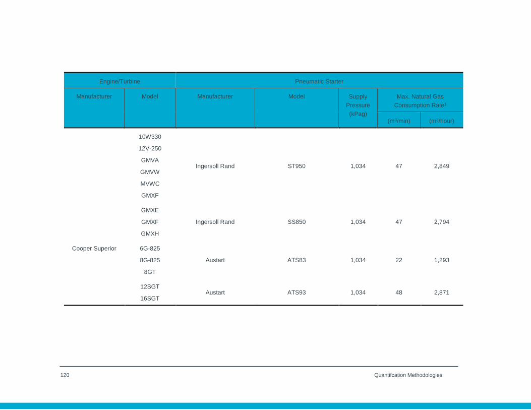
120 Quantifcation Methodologies
Engine/Turbine Pneumatic Starter
Manufacturer Model Manufacturer Model Supply
Pressure
(kPag)
Max. Natural Gas
Consumption Rate1
(m3/min) (m3/hour)
10W330
12V-250
GMVA
GMVW
MVWC
GMXF
Ingersoll Rand ST950 1,034 47 2,849
GMXE
GMXF
GMXH
Ingersoll Rand SS850 1,034 47 2,794
Cooper Superior
6G-825
8G-825
8GT
Austart ATS83 1,034 22 1,293
12SGT
16SGT Austart ATS93 1,034 48 2,871
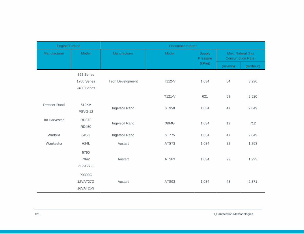
121 Quantifcation Methodologies
Engine/Turbine Pneumatic Starter
Manufacturer Model Manufacturer Model Supply
Pressure
(kPag)
Max. Natural Gas
Consumption Rate1
(m3/min) (m3/hour)
825 Series
1700 Series
2400 Series
Tech Development T112-V 1,034 54 3,226
T121-V 621 59 3,520
Dresser-Rand 512KV
PSVG-12 Ingersoll Rand ST950 1,034 47 2,849
Int Harvester RD372
RD450 Ingersoll Rand 3BMG 1,034 12 712
Wartsila 34SG Ingersoll Rand ST775 1,034 47 2,849
Waukesha
H24L Austart ATS73 1,034 22 1,293
5790
7042
8LAT27G
Austart ATS83 1,034 22 1,293
P9390G
12VAT27G
16VAT25G
Austart ATS93 1,034 48 2,871
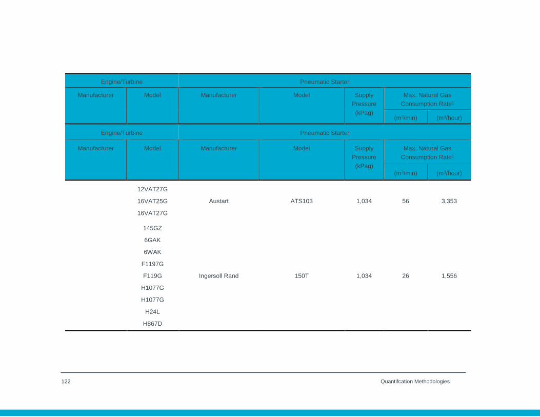
122 Quantifcation Methodologies
Engine/Turbine Pneumatic Starter
Manufacturer Model Manufacturer Model Supply
Pressure
(kPag)
Max. Natural Gas
Consumption Rate1
(m3/min) (m3/hour)
Engine/Turbine Pneumatic Starter
Manufacturer Model Manufacturer Model Supply
Pressure
(kPag)
Max. Natural Gas
Consumption Rate1
(m3/min) (m3/hour)
12VAT27G
16VAT25G
16VAT27G
Austart ATS103 1,034 56 3,353
145GZ
6GAK
6WAK
F1197G
F119G
H1077G
H1077G
H24L
H867D
Ingersoll Rand 150T 1,034 26 1,556
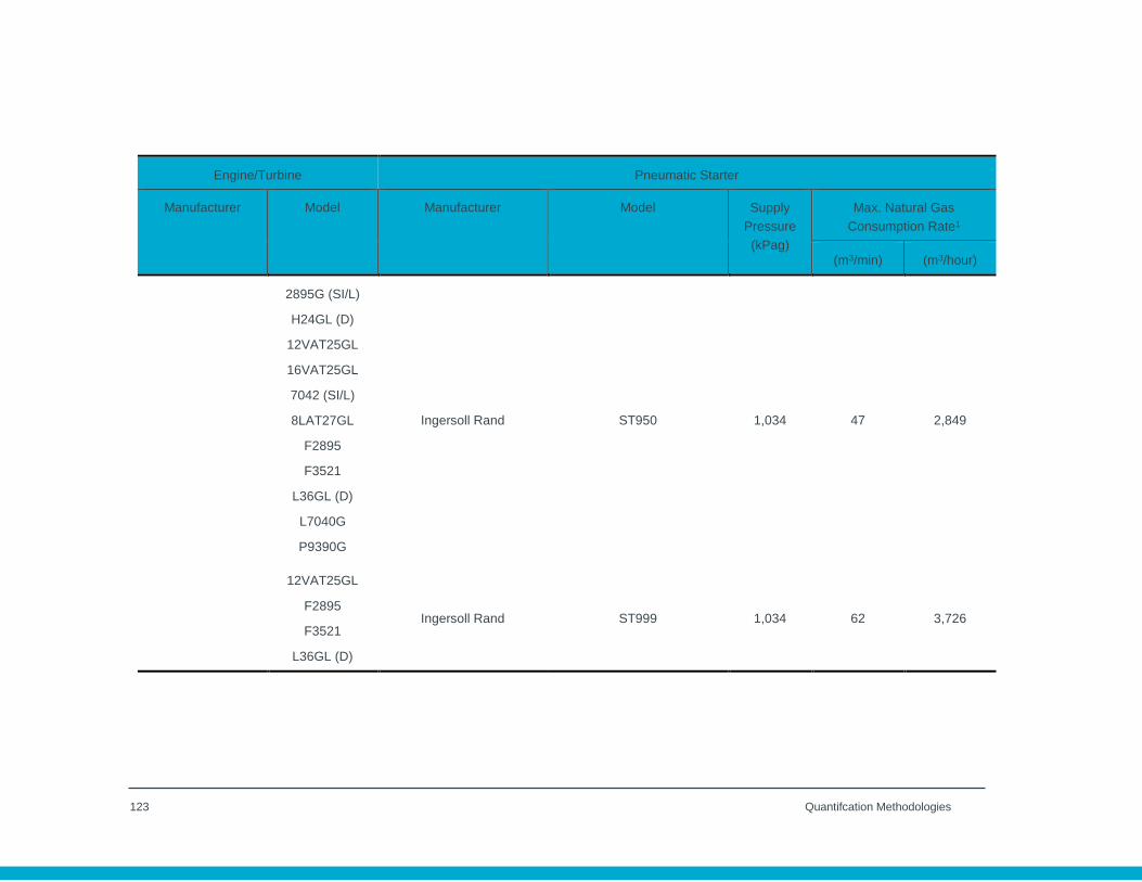
123 Quantifcation Methodologies
Engine/Turbine Pneumatic Starter
Manufacturer Model Manufacturer Model Supply
Pressure
(kPag)
Max. Natural Gas
Consumption Rate1
(m3/min) (m3/hour)
2895G (SI/L)
H24GL (D)
12VAT25GL
16VAT25GL
7042 (SI/L)
8LAT27GL
F2895
F3521
L36GL (D)
L7040G
P9390G
Ingersoll Rand ST950 1,034 47 2,849
12VAT25GL
F2895
F3521
L36GL (D)
Ingersoll Rand ST999 1,034 62 3,726
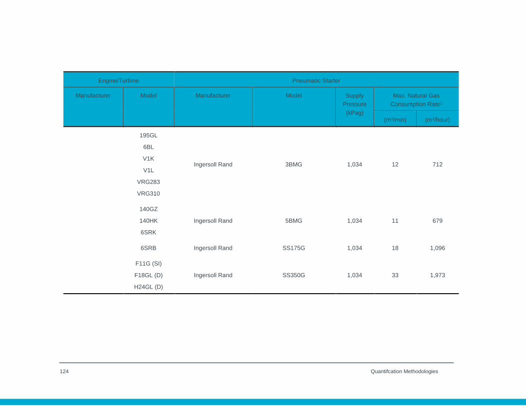
124 Quantifcation Methodologies
Engine/Turbine Pneumatic Starter
Manufacturer Model Manufacturer Model Supply
Pressure
(kPag)
Max. Natural Gas
Consumption Rate1
(m3/min) (m3/hour)
195GL
6BL
V1K
V1L
VRG283
VRG310
Ingersoll Rand 3BMG 1,034 12 712
140GZ
140HK
6SRK
Ingersoll Rand 5BMG 1,034 11 679
6SRB Ingersoll Rand SS175G 1,034 18 1,096
F11G (SI)
F18GL (D)
H24GL (D)
Ingersoll Rand SS350G 1,034 33 1,973
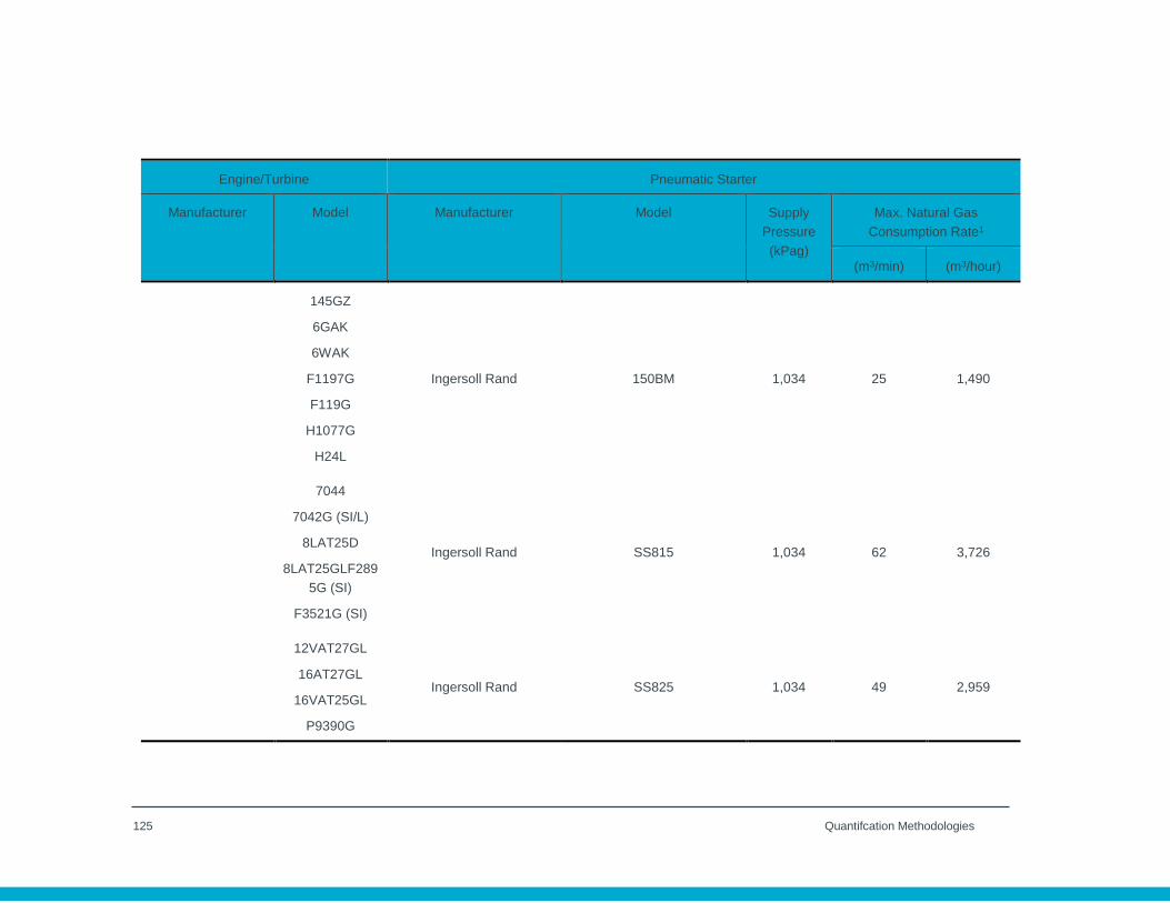
125 Quantifcation Methodologies
Engine/Turbine Pneumatic Starter
Manufacturer Model Manufacturer Model Supply
Pressure
(kPag)
Max. Natural Gas
Consumption Rate1
(m3/min) (m3/hour)
145GZ
6GAK
6WAK
F1197G
F119G
H1077G
H24L
Ingersoll Rand 150BM 1,034 25 1,490
7044
7042G (SI/L)
8LAT25D
8LAT25GLF289
5G (SI)
F3521G (SI)
Ingersoll Rand SS815 1,034 62 3,726
12VAT27GL
16AT27GL
16VAT25GL
P9390G
Ingersoll Rand SS825 1,034 49 2,959

126 Quantifcation Methodologies
Engine/Turbine Pneumatic Starter
Manufacturer Model Manufacturer Model Supply
Pressure
(kPag)
Max. Natural Gas
Consumption Rate1
(m3/min) (m3/hour)
Engine/Turbine Pneumatic Starter
Manufacturer Model Manufacturer Model Supply
Pressure
(kPag)
Max. Natural Gas
Consumption Rate1
(m3/min) (m3/hour)
L5788
L5040
L7042G
L7044G
Tech Development
T112-B 621 57 3,419
T121-B 1,034 5 298
8LAT27G
12VAT25G
12VAT27G
16VAT27G
P9390G
Tech Development
T112-V 1,034 54 3,226
T121-V 621 59 3,520
White RXC
RXLD
RXLX
Ingersoll Rand 5BMG 1,034 11 679

127 Quantifcation Methodologies
Engine/Turbine Pneumatic Starter
Manufacturer Model Manufacturer Model Supply
Pressure
(kPag)
Max. Natural Gas
Consumption Rate1
(m3/min) (m3/hour)
TDXC
This table is adapted from Tables 28 and 29 of AER Manual 015: Estimating Methane Emissions for Reporting to the AER, December 2018.

128 Quantifcation Methodologies
4.20 Non-Routine Venting-Pressure Relief
(1) Introduction
GHG emissions may be vented to the atmosphere during pressure relief events when the relief
system discharges a stream to atmosphere instead of to a flare or vent gas capture system.
Quantification of these emissions require an estimation of the relief rate from the process system
and a measurement or estimation of the composition of the fluid.
Different methods can be used to calculate GHG emissions from pressure relief depending on a
number of factors, including the phase of the fluid being relieved: gas or vapor relief, two-phase
relief, or liquid relief. Emissions may be relieved to atmosphere in two-phases (liquid and gas) in
installations such as in liquefied gas storage, refrigerant systems, or gas operations at high
pressure. When the fluid inside the process equipment is a liquid, GHG emissions may be
released if the liquid contains GHG components and will remain a liquid at atmospheric
temperature and pressure conditions (e.g. certain refrigerants) but the discharged liquid pool will
slowly evaporate. The liquid stream may also contain dissolved or entrained gaseous GHGs like
methane which are released when the relief flow is depressurized to atmosphere.
For pressure relief from rupture discs it is often necessary to perform an unsteady-state
calculation to determine the quantity released, because unlike with a conventional or pilot
operated PSV, the system pressure will decrease after the initial disc rupture as the system loses
inventory, which results in a decreasing flow rate over time. The flow rate should be calculated for
each second following the disc rupture using pressure data from a facility’s process data historian
when available, and these values are then added up over the duration of the relief event in order
to obtain the total relief quantity. Where accurate relief pressure data is not available, the relief
quantity may be estimated by performing a mass balance around the process system to
determine the inventory lost during the pressure relief event. This method may also be employed
if isolation valves are used to automatically isolate a process system upon activation of a rupture
disc device.
Different calculation approaches will be required for gas vented at sonic velocity, known as critical
or choked flow, or below that rate. Relief system hydraulic resistance will need to be determined
using manufacturer data for unique components, and standard values for common components.
Estimation of GHG emissions from venting of atmospheric and low-pressure storage tanks is not
covered in this section. Refer to Section 4.5 for details on how to estimate GHG emissions from
storage tanks.

129 Quantifcation Methodologies
(2) Equations
Calculation methods based on industry best practices should be used for venting emissions from
relief systems, such as those detailed in “Sizing, Selection and Installation of Pressure-Relieving
Instruments, Part I: Sizing and selection. API Standard 520. 9th ed.”, American Petroleum
Institute, July 2014. The following are additional reference documents:
“Technical Paper No.410 – Metric Edition: Flow of Fluids Through Valves, Fittings, and Pipe”
Crane Valves North America. 1999.
”Sizing Pressure-Relief Instruments”, Daniel A. Crowl and Scott A. Tipler, Chemical Engineer
Progress, October 2013, American Institute of Chemical Engineers.
Other methodologies developed by consensus based standards organizations may also be used.
Under CCIR, the selected methodologies must be documented in the facility’s quantification
methodologies document (QMD).
(3) Data requirements
Actual process temperature and pressure conditions should be used when calculating GHG
emissions for each pressure relief event. Engineering estimates should be used if process
data is unavailable.
The composition, physical and transport properties of relief fluids should either be directly
measured or estimated based on process knowledge and/or engineering estimates.
Volumes of process equipment should be calculated directly from isometric drawings as well
as vessel and equipment detail drawings.
4.21 Other Venting Emission Sources
(1) Introduction
Alternative quantification methods may be used for routine or non-routine vent gas sources that
are not covered in the previous sections. This may include vent gas sources that are similar to
ones described in this chapter, but operate under different process conditions.
(2) Equations
A facility may select an appropriate methodology based on the facility's tier classification:

130 Quantifcation Methodologies
Tier 1:
Vent or emission rates based on manufacturer specifications; or
Vent or emission rates from publicly available studies that are specific for the device or type
of vent source.
Tier 2:
Engineering estimates based on, but not limited to mass balances, models, process
knowledge, and facility specific data.
Tier 3:
Periodic (non-continuous) measurements of individual emission sources at normal operating
conditions.
Tier 4:
Continuous measurement of individual emission sources using a permanent or portable
meter.
(3) Data requirements
The facility is required to document the method(s) selected for each vent gas source(s)
including the relevant methodology parameters and assumptions used. For facilities reporting
under CCIR, the documentation of the selected method should be documented in the facility's
QMD.
131 Quantifcation Methodologies
5.0 Quantification Methods for On-Site Transportation
5.1 Introduction
On-site transportation emissions are direct emissions resulting from fuel combustion in machinery
and mobile equipment used for on-site transportation of products and materials integral to the
production process of a facility and any other form of transportation taking place within the facility
boundary.
Examples of on-site transportation include:
Transportation of raw or intermediate products and materials within the production process
such as equipment used at an oil sands operation to mine and/or move materials to
subsequent on-site processing;
Equipment used at above or below ground mining operations to mine and/or move mined
materials;
Equipment used to transport intermediate products or materials to different on-site production
processes;
Equipment used to handle or load final product for transport, including movement or
management of inventory prior to final shipment outside of facility boundaries;
Transportation of by-products or wastes, such as mining overburden or tailings; and
Motor vehicle usage on site for general transportation purposes (including transport of
people) for regulated facilities under the Carbon Competitiveness Incentive Regulation
(CCIR).
Quantification methodologies for on-site transportation emissions are similar to those methods
prescribed in Chapter 1 Stationary Fuel Combustion and are referenced throughout this chapter.
Under the CCIR, specified gas emissions from the combustion of fuels that are exempted from
the carbon levy must be reported in a facility's compliance reports. Emissions that are priced
under the carbon levy are subtracted from the facility's total regulated emissions (TRE).
Specifically for the period up to May 31, 2019, emissions from unmarked fuels are subtracted
from the TRE; while emissions subsequent to this date are included in the TRE. Therefore,
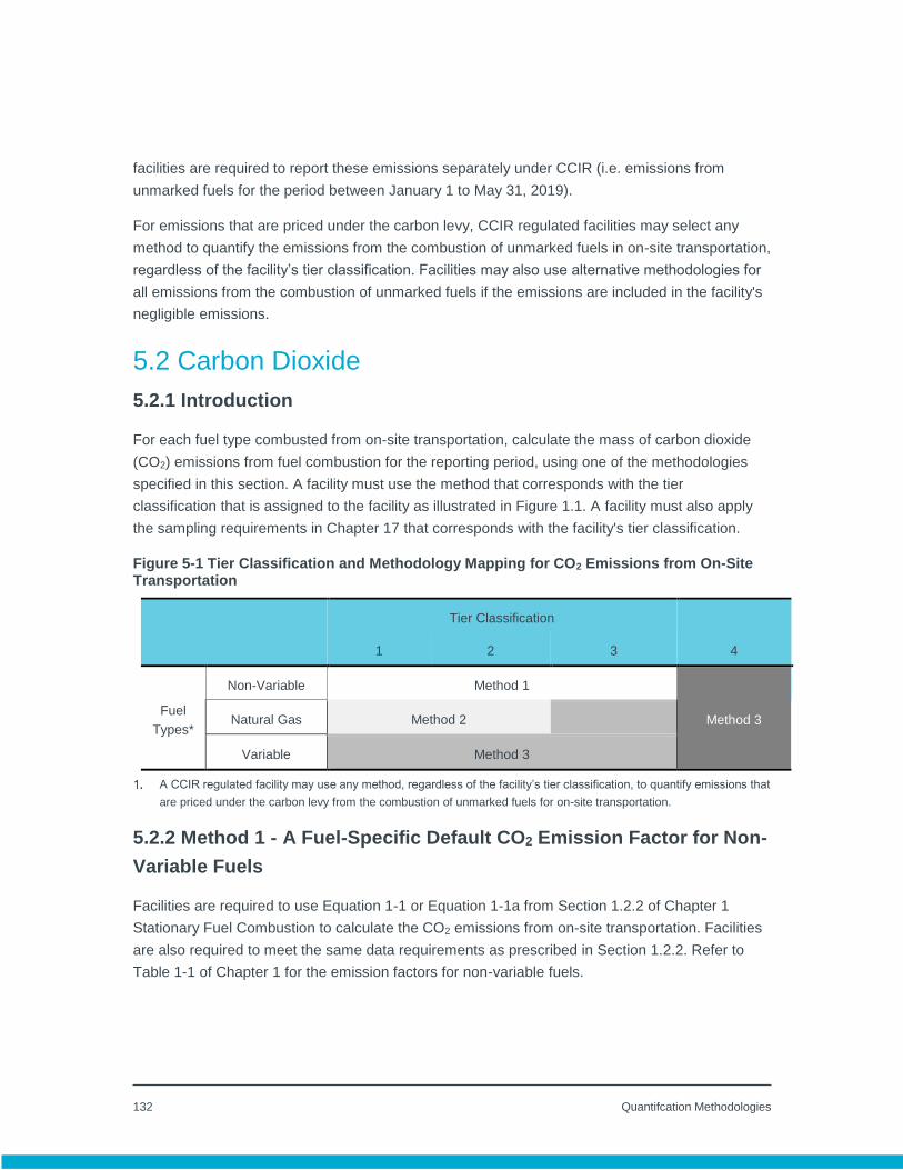
132 Quantifcation Methodologies
facilities are required to report these emissions separately under CCIR (i.e. emissions from
unmarked fuels for the period between January 1 to May 31, 2019).
For emissions that are priced under the carbon levy, CCIR regulated facilities may select any
method to quantify the emissions from the combustion of unmarked fuels in on-site transportation,
regardless of the facility’s tier classification. Facilities may also use alternative methodologies for
all emissions from the combustion of unmarked fuels if the emissions are included in the facility's
negligible emissions.
5.2 Carbon Dioxide
5.2.1 Introduction
For each fuel type combusted from on-site transportation, calculate the mass of carbon dioxide
(CO2) emissions from fuel combustion for the reporting period, using one of the methodologies
specified in this section. A facility must use the method that corresponds with the tier
classification that is assigned to the facility as illustrated in Figure 1.1. A facility must also apply
the sampling requirements in Chapter 17 that corresponds with the facility's tier classification.
Figure 5-1 Tier Classification and Methodology Mapping for CO2 Emissions from On-Site Transportation
Tier Classification
1 2 3 4
Fuel
Types*
Non-Variable Method 1
Method 3 Natural Gas Method 2
Variable Method 3
A CCIR regulated facility may use any method, regardless of the facility’s tier classification, to quantify emissions that
are priced under the carbon levy from the combustion of unmarked fuels for on-site transportation.
5.2.2 Method 1 - A Fuel-Specific Default CO2 Emission Factor for Non-
Variable Fuels
Facilities are required to use Equation 1-1 or Equation 1-1a from Section 1.2.2 of Chapter 1
Stationary Fuel Combustion to calculate the CO2 emissions from on-site transportation. Facilities
are also required to meet the same data requirements as prescribed in Section 1.2.2. Refer to
Table 1-1 of Chapter 1 for the emission factors for non-variable fuels.

133 Quantifcation Methodologies
These emissions do not include CO2 emissions from biomass combustion. For blended fuels
such as gasoline and diesel, a facility may use the "Diesel in Alberta" and/or "Gasoline in Alberta"
to account for the minimum biofuel content. Facilities may also apply Method 3 (below) to account
for actual biofuel content in diesel and/or gasoline usage for on-site transportation.
5.2.3 Method 2 - CO2 Emissions from Combustion of Natural Gas
Facilities are required to use Equation 1-2 from Section 1.2.3 of Chapter 1 Stationary Fuel
Combustion to calculate the CO2 emissions from on-site transportation. Facilities are also
required to meet the same data requirements as prescribed in Section 1.2.3.
5.2.4 Method 3 - CO2 Emissions from Variable Fuels Based on the
Measured Fuel Carbon Content
Facilities are required to use Equation 1-3c from Section 1.2.4 of Chapter 1 Stationary Fuel
Combustion to calculate the CO2 emissions from on-site transportation using variable fuels.
Facilities are also required to meet the same data requirements as prescribed in Section 1.2.4.
5.3 Methane and Nitrous Oxide
5.3.1 Introduction
Calculate the methane (CH4) and nitrous oxide (N2O) mass emissions for the reporting period
from on-site transportation emissions, for each fuel type including biomass fuels, using the
methods specified in this section. Figure 5-2 provides the requirements for facilities based on tier
classification.
Figure 5-2 Requirements Based on Tier Classification
Tier Classification
1 2 3
Requirements
Method 1 using emission factors
from Table 1-1 (Chapter 1
Stationary Fuel Combustion)
and/or Table 5-1
Method 1 using emission factors from Table 5-1
A CCIR regulated facility may use any method, regardless of the facility’s tier classification, to quantify emissions that
are priced under the carbon levy from the combustion of unmarked fuels for on-site transportation.
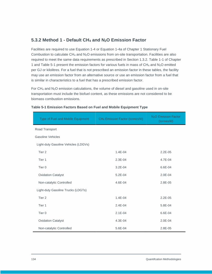
134 Quantifcation Methodologies
5.3.2 Method 1 - Default CH4 and N2O Emission Factor
Facilities are required to use Equation 1-4 or Equation 1-4a of Chapter 1 Stationary Fuel
Combustion to calculate CH4 and N2O emissions from on-site transportation. Facilities are also
required to meet the same data requirements as prescribed in Section 1.3.2. Table 1-1 of Chapter
1 and Table 5-1 present the emission factors for various fuels in mass of CH4 and N2O emitted
per GJ or kilolitres. For a fuel that is not prescribed an emission factor in these tables, the facility
may use an emission factor from an alternative source or use an emission factor from a fuel that
is similar in characteristics to a fuel that has a prescribed emission factor.
For CH4 and N2O emission calculations, the volume of diesel and gasoline used in on-site
transportation must include the biofuel content, as these emissions are not considered to be
biomass combustion emissions.
Table 5-1 Emission Factors Based on Fuel and Mobile Equipment Type
Type of Fuel and Mobile Equipment CH4 Emission Factor (tonnes/kl) N2O Emission Factor
(tonnes/kl)
Road Transport
Gasoline Vehicles
Light-duty Gasoline Vehicles (LDGVs)
Tier 2 1.4E-04 2.2E-05
Tier 1 2.3E-04 4.7E-04
Tier 0 3.2E-04 6.6E-04
Oxidation Catalyst 5.2E-04 2.0E-04
Non-catalytic Controlled 4.6E-04 2.8E-05
Light-duty Gasoline Trucks (LDGTs)
Tier 2 1.4E-04 2.2E-05
Tier 1 2.4E-04 5.8E-04
Tier 0 2.1E-04 6.6E-04
Oxidation Catalyst 4.3E-04 2.0E-04
Non-catalytic Controlled 5.6E-04 2.8E-05
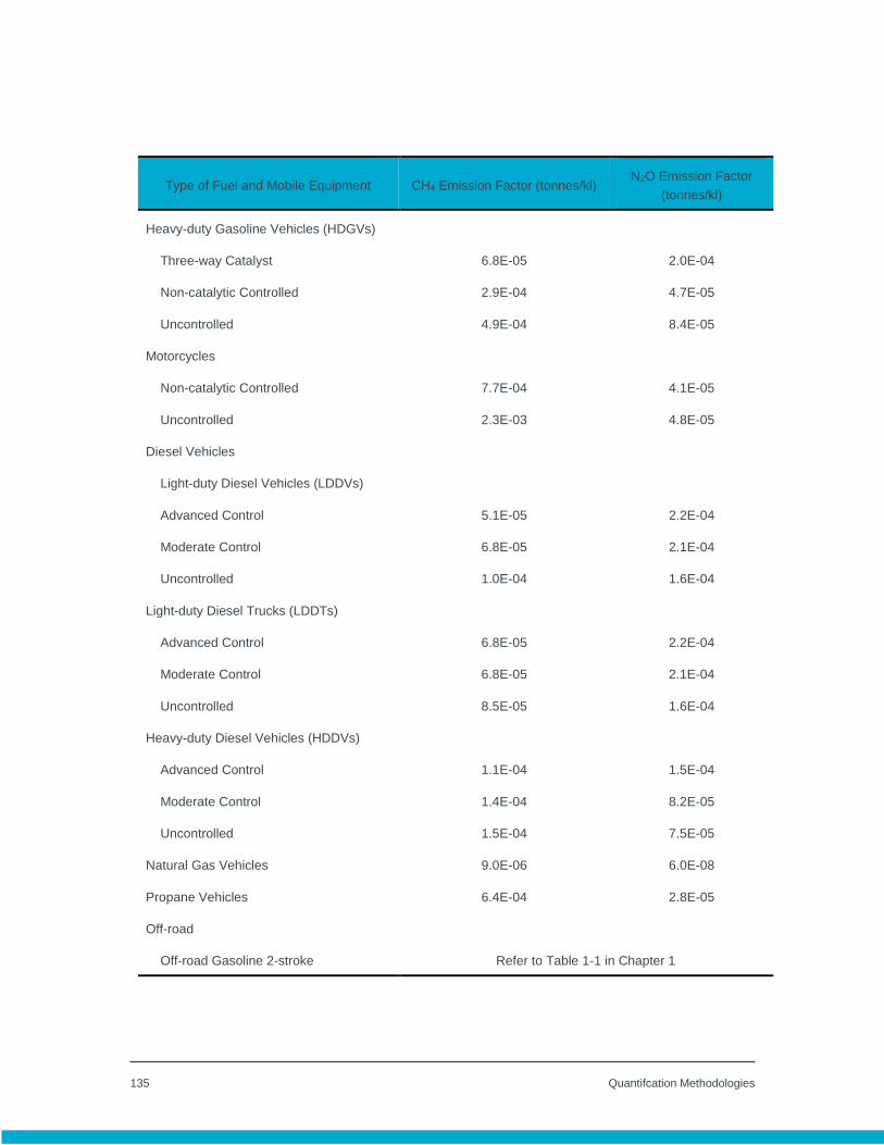
135 Quantifcation Methodologies
Type of Fuel and Mobile Equipment CH4 Emission Factor (tonnes/kl) N2O Emission Factor
(tonnes/kl)
Heavy-duty Gasoline Vehicles (HDGVs)
Three-way Catalyst 6.8E-05 2.0E-04
Non-catalytic Controlled 2.9E-04 4.7E-05
Uncontrolled 4.9E-04 8.4E-05
Motorcycles
Non-catalytic Controlled 7.7E-04 4.1E-05
Uncontrolled 2.3E-03 4.8E-05
Diesel Vehicles
Light-duty Diesel Vehicles (LDDVs)
Advanced Control 5.1E-05 2.2E-04
Moderate Control 6.8E-05 2.1E-04
Uncontrolled 1.0E-04 1.6E-04
Light-duty Diesel Trucks (LDDTs)
Advanced Control 6.8E-05 2.2E-04
Moderate Control 6.8E-05 2.1E-04
Uncontrolled 8.5E-05 1.6E-04
Heavy-duty Diesel Vehicles (HDDVs)
Advanced Control 1.1E-04 1.5E-04
Moderate Control 1.4E-04 8.2E-05
Uncontrolled 1.5E-04 7.5E-05
Natural Gas Vehicles 9.0E-06 6.0E-08
Propane Vehicles 6.4E-04 2.8E-05
Off-road
Off-road Gasoline 2-stroke Refer to Table 1-1 in Chapter 1
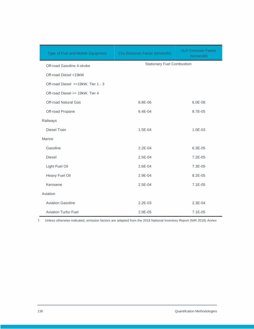
136 Quantifcation Methodologies
Type of Fuel and Mobile Equipment CH4 Emission Factor (tonnes/kl) N2O Emission Factor
(tonnes/kl)
Off-road Gasoline 4-stroke Stationary Fuel Combustion
Off-road Diesel <19kW
Off-road Diesel >=19kW, Tier 1 - 3
Off-road Diesel >= 19kW, Tier 4
Off-road Natural Gas 8.8E-06 6.0E-08
Off-road Propane 6.4E-04 8.7E-05
Railways
Diesel Train 1.5E-04 1.0E-03
Marine
Gasoline 2.2E-04 6.3E-05
Diesel 2.5E-04 7.2E-05
Light Fuel Oil 2.6E-04 7.3E-05
Heavy Fuel Oil 2.9E-04 8.2E-05
Kerosene 2.5E-04 7.1E-05
Aviation
Aviation Gasoline 2.2E-03 2.3E-04
Aviation Turbo Fuel 2.9E-05 7.1E-05
Unless otherwise indicated, emission factors are adapted from the 2018 National Inventory Report (NIR 2018) Annex

137 Quantifcation Methodologies
8.0 Quantification of Industrial Process Emissions
8.1 Introduction
Industrial process (IP) emissions are direct emissions of specified gases generated from an
industrial process involving chemical or physical reactions other than combustion, and where the
primary purpose of the industrial process is not energy production. Emissions from the
unavoidable combustion of carbon black in production of carbon black and ethylene in production
of ethylene oxide are also included as IP emissions. IP emissions are typically generated from
processes in chemical, mineral, and metal production. This chapter is used for the following
industrial process sources:
CO2 from Hydrogen Production;
CO2 from Calcining Mineral Carbonates;
CO2 from Carbonate Use;
CO2 from Ethylene Oxide Production;
CO2 from Thermal Carbon Black Production;
CO2 from Carbon Consumption; and
N2O from Nitric Acid Production.
Facilities that generate industrial process emissions from a source that is not included in this
chapter may use a method that is based on facility specific data or engineering estimates. The
methodology used to calculate these emissions must be included in the facility's Quantification
Methodology Document (QMD) for reporters under the CCIR.
In this chapter, there may be one or more methodologies prescribed for a process that are not
tiered and therefore, are considered to be acceptable for use by a facility under any tier
classification.

138 Quantifcation Methodologies
8.2 CO2 from hydrogen production
8.2.1 Introduction
Hydrogen is produced at bitumen upgraders, petroleum refineries, chemical plants, stand alone
facilities and fertilizer plants, where it is needed for purification or synthesis of substances. In
Alberta, hydrogen is produced from gaseous hydrocarbon feeds (typically natural gas) through a
process of steam-methane reforming (SMR), followed by shift reactions. The primary and
secondary reforming reactions produce carbon monoxide (CO) and hydrogen (H2). Subsequent
shift reactions convert CO to CO2 to produce additional hydrogen. CO2 is a by-product of the net
reaction:
Steam Methane Reforming: CH4 + H2O CO + 3H2
Shift Reaction: CO + H2O CO2 + H2
Overall Reaction: CH4 + 2H2O CO2 + 4H2
Any CO2 generated as a by-product of the above reaction is considered an IP emission.
However, under the SGRR these by-product CO2 emissions must be reported as venting
emission instead of IP, if the hydrogen production is at a fossil fuel production or processing
facility, such as an upgrader or refinery. This is aligned with requirements of Canada’s
Greenhouse Gas Reporting Program. The CO2 by-product produced through reaction can be
removed by physical adsorption (e.g. Pressure-Swing Adsorption, PSA) or chemical absorption
(e.g. amines, potassium carbonate).
Please note that hydrogen can also be generated through the partial oxidation of hydrocarbons to
synthesis gas (“syngas” containing CO and H2). This process can occur as shown in the first
equation above (steam-methane reforming) or the same reaction with pure oxygen added, as
follows:
Partial Oxidation Reaction: HCs + H2O + O2 xCO + yH2 + CO2(trace)
As above, any CO2 generated as a by-product of the above reaction are considered an IP
emission. Syngas can be combusted as a fuel but the CO2 generated from syngas combustion
are considered stationary fuel combustion emissions and must be reported under that source
category.
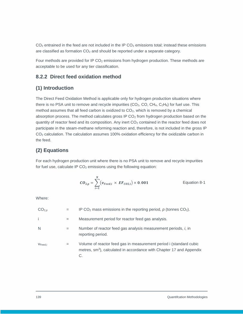
139 Quantifcation Methodologies
CO2 entrained in the feed are not included in the IP CO2 emissions total; instead these emissions
are classified as formation CO2 and should be reported under a separate category.
Four methods are provided for IP CO2 emissions from hydrogen production. These methods are
acceptable to be used for any tier classification.
8.2.2 Direct feed oxidation method
(1) Introduction
The Direct Feed Oxidation Method is applicable only for hydrogen production situations where
there is no PSA unit to remove and recycle impurities (CO2, CO, CH4, C2H6) for fuel use. This
method assumes that all feed carbon is oxidized to CO2, which is removed by a chemical
absorption process. The method calculates gross IP CO2 from hydrogen production based on the
quantity of reactor feed and its composition. Any inert CO2 contained in the reactor feed does not
participate in the steam-methane reforming reaction and, therefore, is not included in the gross IP
CO2 calculation. The calculation assumes 100% oxidation efficiency for the oxidizable carbon in
the feed.
(2) Equations
For each hydrogen production unit where there is no PSA unit to remove and recycle impurities
for fuel use, calculate IP CO2 emissions using the following equation:
𝑪𝑶𝟐,𝒑 = ∑(𝝊𝑭𝒆𝒆𝒅,𝒊 × 𝑬𝑭𝑪𝑶𝟐,𝒊)
𝑵
𝒊=𝟏
× 𝟎. 𝟎𝟎𝟏 Equation 8-1
Where:
CO2,p = IP CO2 mass emissions in the reporting period, p (tonnes CO2).
i = Measurement period for reactor feed gas analysis.
N = Number of reactor feed gas analysis measurement periods, i, in
reporting period.
νFeed,i = Volume of reactor feed gas in measurement period i (standard cubic
metres, sm3), calculated in accordance with Chapter 17 and Appendix
C.

140 Quantifcation Methodologies
EFCO2,i = Feed-specific CO2 emission factor calculated from the measured
reactor feed gas composition analysis results for measurement period i
(kgCO2/sm3) as defined by Equation 8-1a.
0.001 = Mass conversion factor (t/kg).
𝑬𝑭𝑪𝑶𝟐,𝒊 = ∑(𝑴𝑭𝒌,𝒊 × 𝑵𝑪𝒌)
𝑲
𝒌=𝟏
× 𝝆𝑪𝑶𝟐 Equation 8-1a
Where:
EFCO2,i = IP CO2 emission factor for measurement period i (kgCO2/sm3).
I = Measurement period for reactor feed gas analysis.
K = Individual carbon-based oxidizable component of reactor feed gas.
K = Number of measured carbon-based, oxidizable components (e.g.
hydrocarbons, CO, COS, CS2) having non-zero molar fractions in feed
gas. Note: CO2 contained in the feed gas is not included.
MFk,i = Mole fraction of carbon-based oxidizable component k in reactor feed
gas in measurement period i. Note: The mole fraction of CO2 contained
in the feed gas is not included.
NCk = Number of carbons contained in carbon-based oxidizable component k
in reactor feed gas.
CO2 = 1.8613 kg/m3 at standard conditions (where CO2 is determined by the
molecular weight of CO2 divided by the molar volume of ideal gas at
standard conditions as defined by Appendix C).
(3) Data requirements
The volume, temperature, pressure and composition of the reactor feed gas must be
measured in accordance with Chapter 17.

141 Quantifcation Methodologies
The volume of the reactor feed gas must be adjusted to the volume at standard conditions as
defined in Appendix C.
8.2.3 CO2 Mass balance method
(1) Introduction
The CO2 Mass Balance Method is typically used in hydrogen production situations where there is
a PSA unit that purifies a raw hydrogen stream by removing all non-hydrogen contaminants
produced in the SMR and shift reactions or where partial oxidation is used for hydrogen
generation. The PSA Purge Gas stream containing CO2, CO, CH4, C2H6, and some waste H2 is
typically recovered and used as a low-HHV fuel gas in the combustion side of the Reformer
Furnace. The method recognizes the following assumptions:
CO2 contained in reaction or imported feed is not counted in the IP CO2 calculation.
(2) Equations
For each hydrogen production unit, calculate IP CO2 emissions using Equation 8-2:
𝑪𝑶𝟐 = 𝑪𝑶𝟐 𝒊𝒏 𝑹𝒂𝒘 𝑼𝒏𝒑𝒖𝒓𝒊𝒇𝒊𝒆𝒅 𝑯𝟐 𝒔𝒕𝒓𝒆𝒂𝒎 − 𝑪𝑶𝟐 𝒊𝒏 𝒇𝒆𝒆𝒅
𝑪𝑶𝟐,𝒑 = [∑(𝝊𝑹𝒂𝒘𝑼 𝑯𝟐,𝒊 × 𝑴𝑭𝑪𝑶𝟐 𝑹𝒂𝒘𝑼 𝑯𝟐,𝒊 − 𝝊𝑭𝒆𝒆𝒅,𝒊 × 𝑴𝑭𝑪𝑶𝟐,𝑭𝒆𝒆𝒅,𝒊)
𝑵
𝒊=𝟏
× 𝝆𝑪𝑶𝟐] × 𝟎. 𝟎𝟎𝟏
Equation 8-2
Where:
CO2,p = IP CO2 mass emissions in the reporting period, p (tonnes CO2)
i = Measurement period for IP CO2.
N = Number of IP CO2 measurement periods i in the reporting period.
νRawU H2,i = Volume of raw unpurified H2 stream in measurement period i (sm3).
νFeed,i = Volume of reactor feed gas in measurement period i (sm3).
MFCO2,Feed,i = CO2 mole fraction in reactor feed gas (kmolCO2/kmolFeed).

142 Quantifcation Methodologies
MFCO2,RawU H2,i = CO2 mole fraction in raw unpurified hydrogen stream
(kmolCO2/kmolRawH2).
CO2 = 1.8613 kg/m3 at standard conditions as defined in Appendix C.
0.001 = Mass conversion factor (t/kg).
(3) Data requirements
The volume, temperature, pressure and composition of the reactor feed gas must be
measured in accordance with Chapter 17.
The volume, temperature, pressure and composition of the raw unpurified hydrogen streams
(i.e. before PSA) must be measured in the same frequency as the reactor feed gas.
The volume of the reactor feed gas and raw unpurified hydrogen stream must be adjusted to
the volume at standard conditions as defined in Appendix C.
8.2.4 Hydrogen feed calculation method
(1) Introduction
The Hydrogen Feed Calculation Method is an alternative method that back-calculates the quantity
of eligible gas feed based on the measured mass of hydrogen generated. This method eliminates
the need to measure intermediate, recycled, and wasted streams and their composition by
focusing on the stoichiometric feed-to-hydrogen molar ratios for each oxidizable component of the
feed gas. The method recognizes the following assumptions:
CO2 contained in reaction feed is not counted in the IP CO2 calculation; and
All hydrogen is generated through full oxidation of carbon contained in hydrocarbons.
(2) Equations
For each hydrogen production unit, calculate IP CO2 emissions using the following equation:
𝑪𝑶𝟐,𝒑 = ∑ (𝝊𝑯𝟐,𝒊
∑ (𝑺𝑹𝑯𝟐/𝑪𝑶𝟐,𝒌 × 𝑴𝑭𝒌,𝒊)𝑲𝒌=𝟏
) × 𝝆𝑪𝑶𝟐 × 𝟎. 𝟎𝟎𝟏
𝑵
𝒊=𝟏
Equation 8-3
Where:

143 Quantifcation Methodologies
CO2,p = IP CO2 mass emissions in the reporting period, p (tonnes CO2).
i = Measurement period for reactor feed gas analysis.
N = Number of reactor feed gas analysis measurement periods i in reporting
period.
k = Carbon-based oxidizable components.
K = Number of carbon-based oxidizable components.
νH2,i = Volume of hydrogen produced in measurement period i (sm3) at
standard conditions as defined in Appendix C.
SRH2/CO2,k = Stoichiometric hydrogen-to-CO2 molar ratio for carbon-based oxidizable
component k (CO, CH4, C2H6, etc.) in reactor feed gas, as listed in
Table 8-1;
MFk,i = Mole fraction of carbon-based oxidizable component k (e.g. CO,
hydrocarbons) in the reactor feed gas in measurement period i. Note:
CO2 and other inert components contained in the reactor feed gas are
not included.
CO2 = 1.8613 kg/m3 at standard conditions as defined in Appendix C.
0.001 = Mass conversion factor (t/kg).
Table 8-1 Stoichiometric Molar Ratios of Hydrogen to CO2
Feed Component Overall Reaction Equation SR: H2/CO2 Molar
Ratio (mol H2/mol
CO2)
Methane CH4 + 2H2O CO2 + 4H2 4/1 = 4.000
Ethylene C2H4 + 4H2O 2CO2 + 6H2 6/2 = 3.000
Ethane C2H6 + 4H2O 2CO2 + 7H2 7/2 = 3.500
Propylene C3H6 + 6H2O 3CO2 + 9H2 9/3 = 3.000
Propane C3H8 + 6H2O 3CO2 + 10H2 10/3 = 3.333

144 Quantifcation Methodologies
Feed Component Overall Reaction Equation SR: H2/CO2 Molar
Ratio (mol H2/mol
CO2)
Butylenes C4H8 + 8H2O 4CO2 + 12H2 12/4 = 3.000
Butanes C4H10 + 8H2O 4CO2 + 13H2 13/4 = 3.250
Pentenes C5H10 + 10H2O 5CO2 + 15H2 15/5 = 3.000
Pentanes C5H12 + 10H2O 5CO2 + 16H2 16/5 = 3.200
Hexanes C6H14 + 12H2O 6CO2 + 19H2 19/6 = 3.167
Heptanes C7H16 + 14H2O 7CO2 + 22H2 22/7 = 3.143
Carbon Monoxide CO + H2O CO2 + H2 1/1 = 1.000
(3) Data requirements
The composition of the reactor feed gas must be measured in accordance with Chapter 17
and Appendix C.
The volume, temperature, pressure and composition of the hydrogen product stream must be
measured in the same frequency as the reactor feed gas.
The volume of the hydrogen product stream must be adjusted to the volume at standard
conditions as defined in Appendix C.
8.2.5 IP CO2 Emissions from Mass Balance
(1) Introduction
Industrial process CO2 emissions from hydrogen production can be determined by a mass
balance approach if the facility's fuel and feed metering system is integrated and the total fuel and
feed consumption can be accurately determined (e.g., third party custody meter). Provided that
the facility uses the required methodologies prescribed in Chapter 1 Stationary Fuel Combustion
to quantify the CO2 emissions from fuel combustion, a mass balance approach can be used to
quantify the IP CO2 emissions, which assumes that all carbon that is not combusted would be
emitted as IP CO2. Similar to above methods, CO2 entrained in the fuel or feed is not included in
the IP CO2 emissions.

145 Quantifcation Methodologies
(2) Equations
For gaseous fuels and feedstocks, where fuel consumption is measured in units of volume (m3),
use Equation 8-4a:
𝑪𝑶𝟐,𝒑 = (𝒗𝒕𝒐𝒕𝒂𝒍,𝒑 − 𝒗𝑺𝑭𝑪,𝒑) × 𝑪𝑪𝒈𝒂𝒔,𝒑 × 𝟑. 𝟔𝟔𝟒 × 𝟎. 𝟎𝟎𝟏 Equation 8-4a
For gaseous fuels and feedstocks, where fuel consumption is measured in units of energy (GJ),
use Equation 8-4b:
𝑪𝑶𝟐,𝒑 =𝑬𝑵𝑬𝒕𝒐𝒕𝒂𝒍,𝒑 − 𝑬𝑵𝑬𝑺𝑭𝑪,𝒑
𝑯𝑯𝑽× 𝑪𝑪𝒈𝒂𝒔,𝒑 × 𝟑. 𝟔𝟔𝟒 × 𝟎. 𝟎𝟎𝟏 Equation 8-4b
Where:
CO2,p = IP CO2 mass emissions in the reporting period, p (tonnes CO2).
vtotal,p = Total volume of feed and fuel supplied to the facility in the reporting
period, p (sm3) calculated in accordance with Chapter 17 and Appendix
C.
vSFC,p = Total volume of fuel that is combusted by the facility in the reporting
period, p (sm3) calculated in accordance with Chapter 17 and Appendix
C.
CCgas,p = Weighted average carbon content of the gaseous fuel during the
reporting period, p, calculated in accordance with Chapter 17 and
Appendix C; however CO2 contained in the feed gas is not included.
CCp is in the units of kilogram of carbon per standard cubic metre of
gaseous fuel (kg C/m3).
ENEtotal,p = Total energy of the total fuel and feed (GJ) supplied to the facility at
standard conditions combusted during reporting period, p, calculated in
accordance with Chapter 17 and Appendix C.
ENESFC,p = Total energy of the fuel combusted (GJ) by the facility at standard
conditions combusted during reporting period, p, calculated in
accordance with Chapter 17 and Appendix C.

146 Quantifcation Methodologies
HHV = Weighted average higher heating value of fuel (GJ/m3) at standard
conditions as
3.664 = Ratio of molecular weights, CO2 to carbon.
0.001 = Mass conversion factor (t/kg).
8.2.6 CO2 Consumption in urea production
(1) Introduction
Urea production is often performed in conjunction with ammonia production in fertilizer plants and
a methodology is included here though this is not necessarily an IP quantity. While steam
methane reforming is required and generates CO2 as IP emissions when producing ammonia,
CO2 is consumed in the urea production process as shown in the following chemical reaction:
2NH3 + CO2 → H2N − CO − NH2 + H2O
(2) Equations
The CO2 emissions consumed in the urea production process must be included in the total
regulated emissions reported under the Carbon Competitiveness Incentive Regulation in
accordance with Equation 8-5:
𝑪𝑶𝟐,𝑼𝒓𝒆𝒂,𝒑 = 𝒎𝑼𝒓𝒆𝒂 ×𝑴𝑾𝑪𝑶𝟐
𝑴𝑾𝑼𝒓𝒆𝒂
× 𝟎. 𝟎𝟎𝟏 Equation 8-5
Where:
CO2, Urea,p = CO2 consumed in urea production in reporting period, p (tonnes CO2).
mUrea = Mass of urea produced during reporting period (kg).
MWUrea = Molecular weight of urea (kg/kmol) (60.06 kg/kmol).
MWCO2 = Molecular weight of CO2 (kg/kmol) (44.01 kg/kmol).
0.001 = Mass conversion factor (t/kg).

147 Quantifcation Methodologies
(3) Data requirements
Urea production must be measured based on measurement systems used for accounting
purposes.
8.2.7 Reporting of waste hydrogen
(1) Introduction
Generated hydrogen that is not used or exported is considered to be waste hydrogen. Waste
hydrogen may be vented, flared, or combusted. The method described below is an optional
method for calculating waste hydrogen. Other site specific methods of estimating waste hydrogen
are also acceptable.
(2) Equations
The equation used to calculate the waste hydrogen is provided by Equation 8-6.
𝑯𝟐,𝑾𝒂𝒔𝒕𝒆,𝒑 = ∑[(𝒎𝑯𝟐,𝑮𝒆𝒏,𝒊
𝑵
𝒊=𝟏
+ 𝒎𝑯𝟐,𝑰𝒎𝒑,𝒊) − (𝒎𝑯𝟐,𝑬𝒙𝒑,𝒊 + 𝒎𝑯𝟐,𝑼𝒔𝒆,𝒊)] Equation 8-6
Where:
H2,Waste,p = Waste H2 generated in the reporting period, p (tonnes H2).
i = Measurement period for H2.
N = Number of H2 measurement periods, i, in the reporting period.
mH2,Gen,i = Mass of H2 generated during period i (tonnes).
mH2,Imp,i = Mass of H2 imported during period i (tonnes).
mH2,Exp,i = Mass of H2 exported during period i (tonnes).
mH2,Use,i = Mass of H2 used during period i (tonnes).
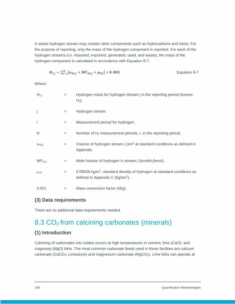
148 Quantifcation Methodologies
A waste hydrogen stream may contain other components such as hydrocarbons and inerts. For
the purpose of reporting, only the mass of the hydrogen component is reported. For each of the
hydrogen streams (i.e. imported, exported, generated, used, and waste), the mass of the
hydrogen component is calculated in accordance with Equation 8-7.
𝑯𝟐,𝒋 = ∑ [𝝊𝑯𝟐,𝒋 × 𝑴𝑭𝑯𝟐,𝒋 × 𝝆𝑯𝟐]𝑵𝒊=𝟏 × 𝟎. 𝟎𝟎𝟏 Equation 8-7
Where:
H2,j = Hydrogen mass for hydrogen stream j in the reporting period (tonnes
H2).
j = Hydrogen stream.
i = Measurement period for hydrogen.
N = Number of H2 measurement periods, i, in the reporting period.
νH2,j = Volume of hydrogen stream j (sm3 at standard conditions as defined in
Appendix
MFH2,j = Mole fraction of hydrogen in stream j (kmolH2/kmol).
H2 = 0.08526 kg/m3, standard density of hydrogen at standard conditions as
defined in Appendix C (kg/sm3).
0.001 = Mass conversion factor (t/kg).
(3) Data requirements
There are no additional data requirements needed.
8.3 CO2 from calcining carbonates (minerals)
(1) Introduction
Calcining of carbonates into oxides occurs at high temperatures in cement, lime (CaO), and
magnesia (MgO) kilns. The most common carbonate feeds used in these facilities are calcium
carbonate (CaCO3; Limestone) and magnesium carbonate (MgCO3). Lime kilns can operate at

149 Quantifcation Methodologies
merchant lime facilities and Kraft pulp mills. The primary reaction equations for calcining of
carbonates are:
Calcium Carbonate: CaCO3 + heat CaO + CO2
Magnesium Carbonate: MgCO3 + heat MgO + CO2
This section is adapted from the guidance provided by the World Business Council for
Sustainable Development (WBCSD) Cement CO2 Protocol (2001) and the Western Climate
Initiative (WCI). One generic method is provided to cover cement, lime, and magnesia kilns. The
contribution from each type of carbonate is accounted for by a composite CO2 emission factor.
The IP CO2 emissions from calcination include only the CO2 generated in the calcining reaction.
Any CO2 generated through the combustion of organic carbon contained in kiln feed materials
creates useful energy and must be calculated using Equation 8-9 and reported under the
Stationary Fuel Combustion source category.
The IP CO2 emissions are calculated as the sum of CO2 emitted from calcination producing the
primary product, P, and the CO2 emitted from calcination producing any waste product from the
kiln. The primary product, P, may be clinker for cement production, quicklime for lime production,
or magnesia for magnesia production. If multiple product grades are produced in one kiln, they
must be weight-averaged into one primary product or their CO2 calculated separately. The waste
product, W, may be cement kiln dust (CKD) for cement production, lime kiln dust (LKD) for lime
production, or magnesia kiln dust (MKD) for magnesia production. The waste product, W, is a
final product from the kiln that is not recycled back to the feed. If multiple waste products are
produced, they must be weight-averaged into one waste product or their CO2 calculated
separately.
(2) Equations
For each kiln, calculate IP CO2 emissions from calcination using the following equation:
𝑪𝑶𝟐−𝑰𝑷,𝒑 = ∑(𝒎𝑷,𝒊 × 𝑬𝑭𝑷,𝒊) +
𝑰
𝒊=𝟏
∑(𝒎𝑾,𝒋 × 𝑬𝑭𝑾,𝒋)
𝑵
𝒋=𝟏
Equation 8-8
Where:

150 Quantifcation Methodologies
CO2-IP,p = IP CO2 mass emissions from calcination of carbonates in reporting
period, p (tonnes CO2).
i = Measurement period i for CaO and MgO in primary product.
I = Number of periods per reporting period for which measurement is
required of CaO and MgO in primary product.
j = Measurement period j for CaO and MgO in waste product.
N = Number of periods per reporting period for which measurement is
required of CaO and MgO in waste product.
P = Primary kiln product.
W = Waste kiln material.
mP,i = Mass of primary kiln product P in measurement period i (tonnes).
EFP,i = CO2 emission factor for primary kiln product P in measurement period i
(tonnes CO2 per tonne P), as defined in Equation 8-8a.
mW,j = Mass of waste kiln material W in measurement period j.
EFW,j = CO2 emission factor for waste kiln material W in measurement period j
(tonnes CO2 per tonne W), as defined in Equation 8-8b.
The kiln-specific CO2 emission factors (EFP,i, EFW,j) are calculated based on the total oxide
content (e.g. CaO, MgO) of the product or waste, less any oxide in that product or waste that
would have been originally present in the feed materials before calcination. These latter oxides
are called “non-calcined” oxides and may be present in fly ash or alternative fuels or raw
materials (AFR).
𝑬𝑭𝑷,𝒊 = (𝑪𝒂𝑶𝑷,𝒊 − 𝑪𝒂𝑶𝑭𝑷,𝒊) × 𝟎. 𝟕𝟖𝟓 + (𝑴𝒈𝑶𝑷,𝒊 − 𝑴𝒈𝑶𝑭𝑷,𝒊) × 𝟏. 𝟎𝟗𝟐 Equation 8-8a
Where:

151 Quantifcation Methodologies
EFP,i = CO2 emission factor for primary kiln product P in measurement period i
(tonnes CO2 per tonne P).
CaOP,i = Total calcium oxide content of primary product P in measurement
period i (tonnes CaO per tonne P).
CaOFP,i = Non-calcined calcium oxide content of primary product P in
measurement period i (tonnes CaO per tonne P), calculated as: fraction
of feed calcium oxide mass allocated to P/mass of P.
MgOP,i = Total magnesium oxide content of primary product P in measurement
period i (tonnes MgO per tonne P).
MgOFP,i = Non-calcined magnesium oxide content of primary product P in
measurement period i (tonnes MgO per tonne P), calculated as: fraction
of feed magnesium oxide mass allocated to P/mass of P;
0.785 = Ratio of molecular weight of CO2 to CaO (44.01/56.1).
1.092 = Ratio of molecular weights of CO2 to MgO (44.01/40.3).
𝑬𝑭𝑾,𝒋 = (𝑪𝒂𝑶𝑾,𝒋 − 𝑪𝒂𝑶𝑭𝑾,𝒋) × 𝟎. 𝟕𝟖𝟓 + (𝑴𝒈𝑶𝑾,𝒋 − 𝑴𝒈𝑶𝑭𝑾,𝒋) × 𝟏. 𝟎𝟗 Equation 8-8b
Where:
EFW,j = CO2 emission factor for waste kiln material W in measurement period j
(tonnes CO2 per tonne W).
CaOW,j = Total calcium oxide content of waste kiln material W in measurement
period j (tonnes CaO per tonne W).
CaOFW,j = Non-calcined calcium oxide content of waste kiln material W in
measurement period j (tonnes CaO per tonne W), calculated as:
fraction of feed calcium oxide mass allocated to W/mass of W.
MgOW,j = Total magnesium oxide content of waste kiln material W in
measurement period j (tonnes MgO per tonne W).

152 Quantifcation Methodologies
MgOFW,j = Non-calcined magnesium oxide content of waste kiln material W in
measurement period j (tonnes MgO per tonne W), calculated as:
fraction of feed magnesium oxide mass allocated to W/mass of W;
magnesium oxide mass allocated to P/mass of P;
0.785 = Ratio of molecular weight of CO2 to CaO (44.01/56.1).
1.092 = Ratio of molecular weights of CO2 to MgO (44.01/40.3).
The CO2 emissions from oxidation of total organic carbon in feed are calculated based on the
carbon content of the feed.
𝑪𝑶𝟐,𝒑 = 𝒎 × 𝑻𝑶𝑪 × 𝟑. 𝟔𝟔𝟒 Equation 8-9
Where:
CO2,p = Fuel combustion CO2 mass emissions from oxidation of feed organic
carbon in the reporting period, p (tonnes CO2).
m = Mass of kiln feed materials (tonnes) in reporting period.
TOC = Total organic carbon content in kiln feed materials (mass fraction);
Default TOC = 0.002 (0.2%);
3.664 = Ratio of molecular weights, CO2 to carbon.
(3) Data requirements
The mass of all feeds and products must be determined monthly from measurement systems
used for accounting purposes for each lime type and each calcined by products/waste type.
Chemical composition of CaO and MgO contents of each lime type and each calcined
byproduct/waste type must be determined during the same month as the production data.
The CaO and MgO content of feed and products must be determined once per month based
on composite samples.
The CaO and MgO content of waste materials must be determined once per quarter.

153 Quantifcation Methodologies
The CaO and MgO content of any material must be determined using: ASTM C25 - Standard
Test Method for Chemical Analysis of Limestone, Quicklime, and Hydrated Lime; or the most
appropriate industry standard method published by a consensus-based standards
organization to determine CaO and MgO content. The reporter should explain the method
used while reporting.
The Total Organic Carbon contained in kiln feeds (TOCF) that is oxidized to CO2 should be
measured once per year, using ASTM C114 or an industry standard method. However, a
default TOCF factor of 0.002 (0.2%) can be used.

154 Quantifcation Methodologies
8.3.2 Lime kilns - Kraft pulp mills
(1) Introduction
Similar to cement, lime, and magnesia kilns, lime kilns are used at Kraft pulp and paper mills. The
emissions generated from these kilns include both industrial process emissions and biomass CO2
emissions. The carbonates in the calcination process, such as sodium carbonate or calcium
carbonate, may be derived from mineral or biomass sources. CO2 emissions that are generated
from the calcination of a biomass-based carbonate materials are classifed as biomass CO2
emissions.
For kilns operating in Kraft pulp mills, the method prescribed to quantify the industrial process
emissions only requires the mass of the starting carbonate material that is mineral based. The
method assumes a default fraction of carbonate reacted of 1.0 (complete reaction). Since the
measurement of unreacted or uncalcined fraction cannot be differentiated between biomass and
mineral-based carbonates, this is not a requirement for this method.
(2) Equations
For any carbonate used, calculate IP CO2 emissions using the following equation:
𝑪𝑶𝟐,𝒑 = ∑(𝒎𝒊 × 𝑬𝑭𝒊 × 𝑭𝒊)
𝑵
𝒊=𝟏
Equation 8-10
Where:
CO2,p = IP CO2 mass emissions from consumption of carbonates in the
reporting period, p (tonnes CO2).
i = Carbonate types.
N = Number of carbonate types.
mi = Mass of carbonate type i consumed that is mineral based (tonnes) in
the reporting period.
EFi = Emission factor for carbonate type i (tonne CO2/tonne carbonate
consumed), from Table 8-2. If an emission factor is not available in
Table 8-2 for a carbonate that is used at the facility, the facility may
155 Quantifcation Methodologies
develop an emission factor based on stoichiometry for the specific
carbonate.
Fi = Fraction reacted for each carbonate type i (mass fraction). A default
value of 1.0 (complete reaction) is assumed. Alternatively, fraction
reacted can be determined by analyzing input and output materials.
(3) Data requirements
The mass of carbonate consumed shall be determined for the reporting period using the
same plant processes used for accounting purposes including purchase records, adjusted for
inventory, or direct measurements.
The mass of carbonates excludes biomass-based carbonates.
8.4 CO2 from use of carbonates
8.4.1 Introduction
CO2 can be generated when carbonates participate in some chemical reactions. Flue gas
desulphurization, pH control of wastewater, acid leaching of ores containing carbonates, and use
of carbonates in metal fluxing are some examples of CO2 generated from carbonate reactions.
8.4.2 Tier 1 - Carbonate consumption method
(1) Introduction
This simplified method is the same as the method prescribed for lime kilns operating in Kraft pulp
mills. The method assumes a default fraction of carbonate reacted of 1.0 (complete reaction).
Measurement of fraction reacted by carbonated analysis is optional.
(2) Equations
Use Equation 8-10 to calculate the IP CO2 emissions.
(3) Data requirements
The mass of carbonate consumed shall be determined for the reporting period using the same
plant processes used for accounting purposes including purchase records, adjusted for inventory,
or direct measurements.
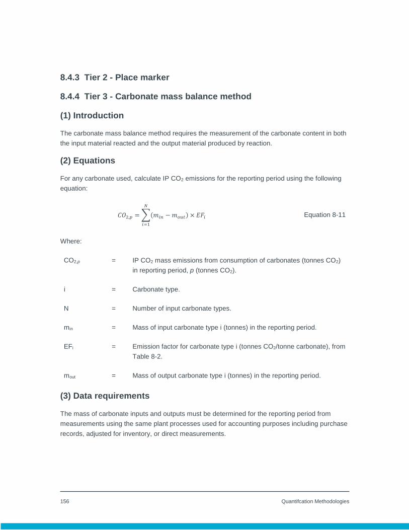
156 Quantifcation Methodologies
8.4.3 Tier 2 - Place marker
8.4.4 Tier 3 - Carbonate mass balance method
(1) Introduction
The carbonate mass balance method requires the measurement of the carbonate content in both
the input material reacted and the output material produced by reaction.
(2) Equations
For any carbonate used, calculate IP CO2 emissions for the reporting period using the following
equation:
𝐶𝑂2,𝑝 = ∑(𝑚𝑖𝑛 − 𝑚𝑜𝑢𝑡) × 𝐸𝐹𝑖
𝑁
𝑖=1
Equation 8-11
Where:
CO2,p = IP CO2 mass emissions from consumption of carbonates (tonnes CO2)
in reporting period, p (tonnes CO2).
i = Carbonate type.
N = Number of input carbonate types.
min = Mass of input carbonate type i (tonnes) in the reporting period.
EFi = Emission factor for carbonate type i (tonnes CO2/tonne carbonate), from
Table 8-2.
mout = Mass of output carbonate type i (tonnes) in the reporting period.
(3) Data requirements
The mass of carbonate inputs and outputs must be determined for the reporting period from
measurements using the same plant processes used for accounting purposes including purchase
records, adjusted for inventory, or direct measurements.

157 Quantifcation Methodologies
Table 8-2 Default Carbonate CO2 Emission Factors
Mineral Name Formula CO2 Emission Factor (tonnes CO2/tonnes
Carbonate)
Limestone CaCO3 0.43971
Magnesite MgCO3 0.52197
Dolomite CaMg(CO3)2 0.47732
Siderite FeCO3 0.37987
Ankerite Ca(Fe,Mg,Mn)(CO3)2 0.47572
Rhodochrosite MnCO3 0.38286
Sodium Carbonate/Soda Ash Na2CO3 0.41492
Others Facility specific emission factor to be
determined through analysis or
supplier information.
8.4.5 Tier 4- Measured CO2 emission factor method
(1) Introduction
CO2 from use of carbonates can be estimated based on a facility-specific CO2 emission factor
measured by an annual stack gas test. This method is only applicable when no other sources of
CO2 contribute to the CO2 in the stack gas from the reaction. CO2 emissions in the reporting
period are calculated by multiplying the activity level of the CO2 generation process in the
reporting period by the measured CO2 emission factor. Activity level data may be based on:
Mass of carbonates consumed; or
Any applicable substance participating in the reaction where CO2 is released.
One example application of this method is the calculation of CO2 emissions from the acid
leaching of different types of ore containing carbonates.
(2) Equations
For an eligible source of CO2 from use of carbonates, calculate IP CO2 emissions in the reporting
period using the following equation:

158 Quantifcation Methodologies
𝐶𝑂2,𝑝 = ∑(𝑚𝑖 × 𝐸𝐹𝑖)
𝑁
𝑖=1
Equation 8-12
Where:
CO2,p = CO2 mass emissions from consumption of carbonates in the reporting
period, p (tonnes CO2).
i = Carbonate-containing material.
N = Number of different carbonate-containing materials.
mi = Mass of carbonate-containing material of type i consumed (tonnes
carbonate) in reporting period.
EFi = CO2 emission factor for carbonate-containing material of type i
(tonnes CO2/tonne carbonate), as determined by Equation 8-13.
𝐸𝐹𝑖 = 𝑀𝐸𝐶𝑂2
𝐴𝐿
Equation 8-13
Where:
MECO2 = CO2 mass emission rate (tonnes CO2/hour), where this value is
determined from stack testing;
AL = Activity level mass rate of carbonate-containing material of type i
(tonnes carbonate/hour) during stack test.
(3) Data requirements
The activity level used in Equation 8-133 must be determined from measurement systems
used for accounting purposes for the period that the stack tests are conducted.
Stack tests to determine EFj must be conducted at least once per year for each different type
of carbonate used or ore treated. A minimum of three test runs for each stack test and hourly
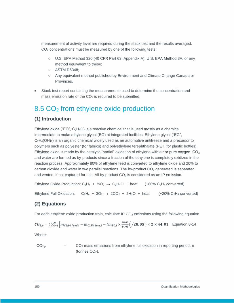
159 Quantifcation Methodologies
measurement of activity level are required during the stack test and the results averaged.
CO2 concentrations must be measured by one of the following tests:
o U.S. EPA Method 320 (40 CFR Part 63, Appendix A), U.S. EPA Method 3A, or any
method equivalent to these;
o ASTM D6348;
o Any equivalent method published by Environment and Climate Change Canada or
Provinces.
Stack test report containing the measurements used to determine the concentration and
mass emission rate of the CO2 is required to be submitted.
8.5 CO2 from ethylene oxide production
(1) Introduction
Ethylene oxide (“EO”, C2H4O) is a reactive chemical that is used mostly as a chemical
intermediate to make ethylene glycol (EG) at integrated facilities. Ethylene glycol (“EG”,
C2H4(OH)2) is an organic chemical widely used as an automotive antifreeze and a precursor to
polymers such as polyester (for fabrics) and polyethylene terephthalate (PET, for plastic bottles).
Ethylene oxide is made by the catalytic “partial” oxidation of ethylene with air or pure oxygen. CO2
and water are formed as by-products since a fraction of the ethylene is completely oxidized in the
reaction process. Approximately 80% of ethylene feed is converted to ethylene oxide and 20% to
carbon dioxide and water in two parallel reactions. The by-product CO2 generated is separated
and vented, if not captured for use. All by-product CO2 is considered as an IP emission.
Ethylene Oxide Production: C2H4 + ½O2 C2H4O + heat (~80% C2H4 converted)
Ethylene Full Oxidation: C2H4 + 3O2 2CO2 + 2H2O + heat (~20% C2H4 converted)
(2) Equations
For each ethylene oxide production train, calculate IP CO2 emissions using the following equation
𝑪𝑶𝟐,𝒑 = ( ∑ [𝒎𝑪𝟐𝑯𝟒 𝒇𝒆𝒆𝒅,𝒊 − 𝒎𝑪𝟐𝑯𝟒 𝒍𝒐𝒔𝒔,𝒊 − (𝒎𝑬𝑶,𝒊 ×𝟐𝟖.𝟎𝟓
𝟒𝟒.𝟎𝟓)] 𝟐𝟖. 𝟎𝟓 )⁄ × 𝟐 × 𝟒𝟒. 𝟎𝟏𝑵
𝒊=𝟏 Equation 8-14
Where:
CO2,p = CO2 mass emissions from ethylene full oxidation in reporting period, p
(tonnes CO2).

160 Quantifcation Methodologies
i = Measurement period.
N = Number of measurement periods in reporting period.
mC2H4 feed,i = Mass of ethylene (C2H4) feed for reaction in measurement period i
(tonne).
mC2H4 loss,i = Mass of ethylene (C2H4) carried out in the waste gas in measurement
period i (tonnes); calculated by Equation 8-14a.
mEO, i = Mass EO produced in period i (tonne), calculated from production of
monoethylene glycol (MEG), diethylene glycol (DEG), and/or
2 = Number of moles of carbon in C2H4.
44.01 = Molecular weight of CO2 (kg/kmol).
28.05 = Molecular weight of C2H4 (kg/kmol).
44.05 = Molecular weight of ethylene oxide (C2H4O) (kg/kmol).
𝒎𝑪𝟐𝑯𝟒,𝒍𝒐𝒔𝒔 = 𝑸𝒗𝒆𝒏𝒕 × 𝑪𝑪𝟐𝑯𝟒/𝟏𝟎𝟎𝟎 Equation 8-14a
Where:
Qvent = Vent gas flow rate in the reporting period (m3).
CC2H4 loss,i = Concentration of the ethylene (kg/m3) in the vent gas based on
measurements.
𝒎𝑬𝑶,𝒑,𝒊 = 𝒎𝑴𝑬𝑮 × 𝟎. 𝟕𝟏𝟎 + 𝒎𝑫𝑬𝑮 × 𝟎. 𝟖𝟑𝟎 + 𝒎𝑻𝑬𝑮 × 𝟎. 𝟖𝟖𝟎 + 𝒎𝑯𝑮 × 𝒂 + 𝒎𝑮𝑾 × 𝒃 Equation 8-14b
Where:
mMEG = Mass of monoethylene glycol production.
0.710 = Ethylene oxide equivalency of monoethylene glycol production.
mDEG = Mass of diethylene glycol production.
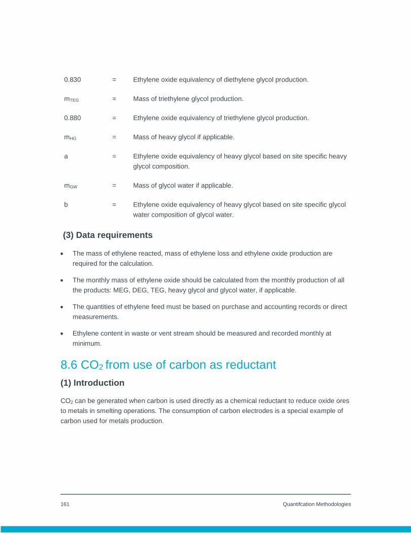
161 Quantifcation Methodologies
0.830 = Ethylene oxide equivalency of diethylene glycol production.
mTEG = Mass of triethylene glycol production.
0.880 = Ethylene oxide equivalency of triethylene glycol production.
mHG = Mass of heavy glycol if applicable.
a = Ethylene oxide equivalency of heavy glycol based on site specific heavy
glycol composition.
mGW = Mass of glycol water if applicable.
b = Ethylene oxide equivalency of heavy glycol based on site specific glycol
water composition of glycol water.
(3) Data requirements
The mass of ethylene reacted, mass of ethylene loss and ethylene oxide production are
required for the calculation.
The monthly mass of ethylene oxide should be calculated from the monthly production of all
the products: MEG, DEG, TEG, heavy glycol and glycol water, if applicable.
The quantities of ethylene feed must be based on purchase and accounting records or direct
measurements.
Ethylene content in waste or vent stream should be measured and recorded monthly at
minimum.
8.6 CO2 from use of carbon as reductant
(1) Introduction
CO2 can be generated when carbon is used directly as a chemical reductant to reduce oxide ores
to metals in smelting operations. The consumption of carbon electrodes is a special example of
carbon used for metals production.
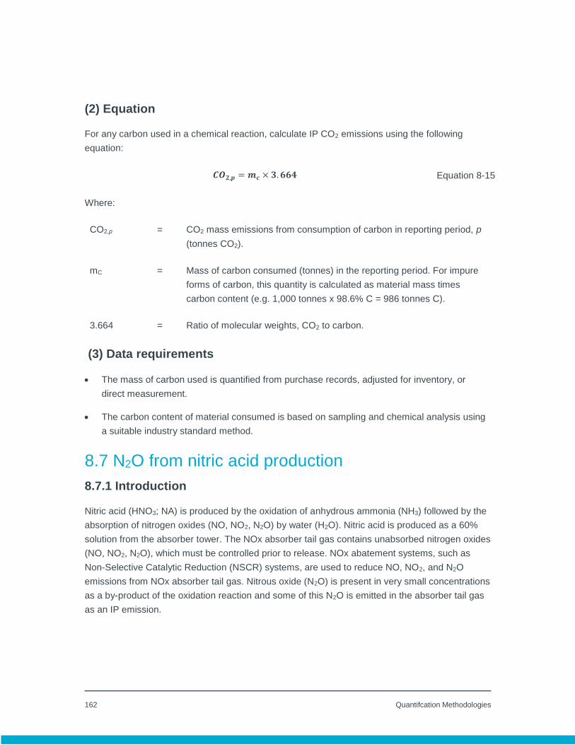
162 Quantifcation Methodologies
(2) Equation
For any carbon used in a chemical reaction, calculate IP CO2 emissions using the following
equation:
𝑪𝑶𝟐,𝒑 = 𝒎𝒄 × 𝟑. 𝟔𝟔𝟒 Equation 8-15
Where:
CO2,p = CO2 mass emissions from consumption of carbon in reporting period, p
(tonnes CO2).
mC = Mass of carbon consumed (tonnes) in the reporting period. For impure
forms of carbon, this quantity is calculated as material mass times
carbon content (e.g. 1,000 tonnes x 98.6% C = 986 tonnes C).
3.664 = Ratio of molecular weights, CO2 to carbon.
(3) Data requirements
The mass of carbon used is quantified from purchase records, adjusted for inventory, or
direct measurement.
The carbon content of material consumed is based on sampling and chemical analysis using
a suitable industry standard method.
8.7 N2O from nitric acid production
8.7.1 Introduction
Nitric acid (HNO3; NA) is produced by the oxidation of anhydrous ammonia (NH3) followed by the
absorption of nitrogen oxides (NO, NO2, N2O) by water (H2O). Nitric acid is produced as a 60%
solution from the absorber tower. The NOx absorber tail gas contains unabsorbed nitrogen oxides
(NO, NO2, N2O), which must be controlled prior to release. NOx abatement systems, such as
Non-Selective Catalytic Reduction (NSCR) systems, are used to reduce NO, NO2, and N2O
emissions from NOx absorber tail gas. Nitrous oxide (N2O) is present in very small concentrations
as a by-product of the oxidation reaction and some of this N2O is emitted in the absorber tail gas
as an IP emission.
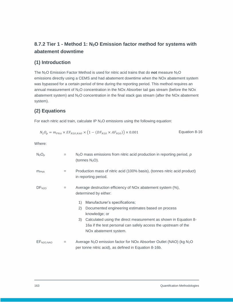
163 Quantifcation Methodologies
8.7.2 Tier 1 - Method 1: N2O Emission factor method for systems with
abatement downtime
(1) Introduction
The N2O Emission Factor Method is used for nitric acid trains that do not measure N2O
emissions directly using a CEMS and had abatement downtime when the NOx abatement system
was bypassed for a certain period of time during the reporting period. This method requires an
annual measurement of N2O concentration in the NOx Absorber tail gas stream (before the NOx
abatement system) and N2O concentration in the final stack gas stream (after the NOx abatement
system).
(2) Equations
For each nitric acid train, calculate IP N2O emissions using the following equation:
𝑁2𝑂𝑝 = 𝑚𝑃𝑁𝐴 × 𝐸𝐹𝑁2𝑂,𝑁𝐴𝑂 × (1 − (𝐷𝐹𝑁2𝑂 × 𝐴𝐹𝑁2𝑂)) × 0.001 Equation 8-16
Where:
N2Op = N2O mass emissions from nitric acid production in reporting period, p
(tonnes N2O).
mPNA = Production mass of nitric acid (100% basis), (tonnes nitric acid product)
in reporting period.
DFN2O = Average destruction efficiency of NOx abatement system (%),
determined by either:
1) Manufacturer’s specifications;
2) Documented engineering estimates based on process
knowledge; or
3) Calculated using the direct measurement as shown in Equation 8-
16a if the test personal can safely access the upstream of the
NOx abatement system.
EFN2O,NAO = Average N2O emission factor for NOx Absorber Outlet (NAO) (kg N2O
per tonne nitric acid), as defined in Equation 8-16b.

164 Quantifcation Methodologies
AFN2O = NOx abatement system operating fraction (%) in the reporting period,
as defined in Equation 8-16c.
0.001 = Mass conversion factor (t/kg).
The average destruction efficiency can be calculated using the following equation:
DFN2O =(𝑪𝑵𝟐𝑶,𝑵𝑨𝑶×𝑸𝑵𝟐𝑶,𝑵𝑨𝑶−𝑪𝑵𝟐𝑶,𝑵𝑨𝑺×𝑸𝑵𝟐𝑶,𝑵𝑨𝑺)
𝑪𝑵𝟐𝑶,𝑵𝑨𝑶×𝑸𝑵𝟐𝑶,𝑵𝑨𝑶 × 𝟏𝟎𝟎% Equation 8-16a
Where:
DFN2O = Average abatement system destruction efficiency (%) in reporting
period.
CN2O,NAO = N2O concentration (ppmv) from the NOx Absorber Outlet (NAO).
QN2O,NAO = Flow rates (m3/h)from the NOx Absorber Outlet (NAO).
CN2O,NAS = N2O concentration (ppmv) from the Nitric Acid Stack (NAS).
QN2O,NAS = Flow rates (m3/h) from the Nitric Acid Stack (NAS).
The train-specific average N2O emission factor is calculated based on direct measurement of N2O
concentration in the NOx Absorber outlet (NAO).
𝑬𝑭𝑵𝟐𝑶,𝑵𝑨𝑶 =
∑𝑸𝑵𝑨𝑶,𝒊 × 𝑪𝑵𝟐𝑶,𝑵𝑨𝑶,𝒊
𝑷𝑹𝑵𝑨,𝒊× 𝟏. 𝟖𝟔𝟏 × 𝟏𝟎−𝟔𝑵
𝒊=𝟏
𝑵
Equation 8-16b
Where:
EFN2O,NAO = Average N2O emission factor for NOx Absorber Outlet (kg N2O per
tonne nitric
i = Test runs.
N = Number of N2O measurement test runs during stack test.
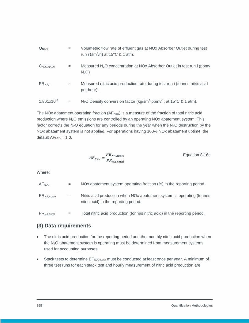
165 Quantifcation Methodologies
QNAO,i = Volumetric flow rate of effluent gas at NOx Absorber Outlet during test
run i (sm3/h) at 15°C & 1 atm.
CN2O,NAO,i = Measured N2O concentration at NOx Absorber Outlet in test run i (ppmv
N2O)
PRNA,i = Measured nitric acid production rate during test run i (tonnes nitric acid
per hour).
1.861x10-6 = N2O Density conversion factor (kg/sm3∙ppmv-1; at 15°C & 1 atm).
The NOx abatement operating fraction (AFN2O) is a measure of the fraction of total nitric acid
production where N2O emissions are controlled by an operating NOx abatement system. This
factor corrects the N2O equation for any periods during the year when the N2O destruction by the
NOx abatement system is not applied. For operations having 100% NOx abatement uptime, the
default AFN2O = 1.0.
𝑨𝑭𝑵𝟐𝑶 =𝑷𝑹𝑵𝑨,𝑨𝒃𝒂𝒕𝒆
𝑷𝑹𝑵𝑨,𝑻𝒐𝒕𝒂𝒍
Equation 8-16c
Where:
AFN2O = NOx abatement system operating fraction (%) in the reporting period.
PRNA,Abate = Nitric acid production when NOx abatement system is operating (tonnes
nitric acid) in the reporting period.
PRNA,Total = Total nitric acid production (tonnes nitric acid) in the reporting period.
(3) Data requirements
The nitric acid production for the reporting period and the monthly nitric acid production when
the N2O abatement system is operating must be determined from measurement systems
used for accounting purposes.
Stack tests to determine EFN2O,NAO must be conducted at least once per year. A minimum of
three test runs for each stack test and hourly measurement of nitric acid production are
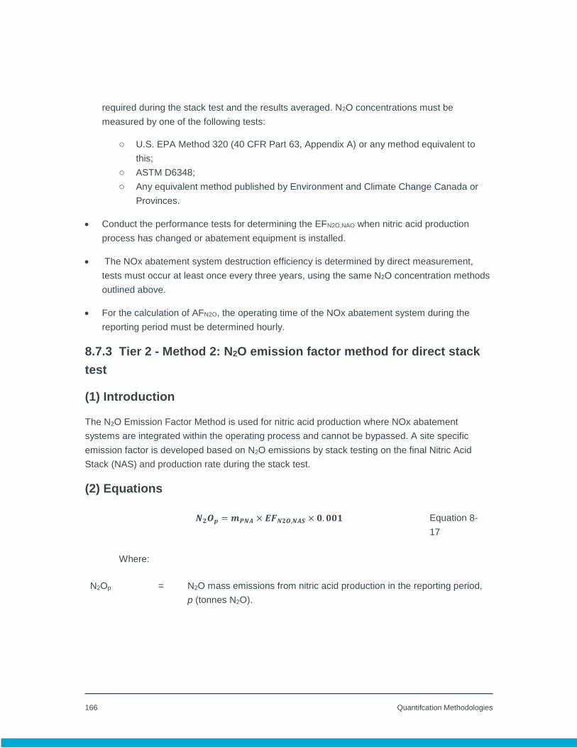
166 Quantifcation Methodologies
required during the stack test and the results averaged. N2O concentrations must be
measured by one of the following tests:
o U.S. EPA Method 320 (40 CFR Part 63, Appendix A) or any method equivalent to
this;
o ASTM D6348;
o Any equivalent method published by Environment and Climate Change Canada or
Provinces.
Conduct the performance tests for determining the EFN2O,NAO when nitric acid production
process has changed or abatement equipment is installed.
The NOx abatement system destruction efficiency is determined by direct measurement,
tests must occur at least once every three years, using the same N2O concentration methods
outlined above.
For the calculation of AFN2O, the operating time of the NOx abatement system during the
reporting period must be determined hourly.
8.7.3 Tier 2 - Method 2: N2O emission factor method for direct stack
test
(1) Introduction
The N2O Emission Factor Method is used for nitric acid production where NOx abatement
systems are integrated within the operating process and cannot be bypassed. A site specific
emission factor is developed based on N2O emissions by stack testing on the final Nitric Acid
Stack (NAS) and production rate during the stack test.
(2) Equations
𝑵𝟐𝑶𝒑 = 𝒎𝑷𝑵𝑨 × 𝑬𝑭𝑵𝟐𝑶,𝑵𝑨𝑺 × 𝟎. 𝟎𝟎𝟏 Equation 8-
17
Where:
N2Op = N2O mass emissions from nitric acid production in the reporting period,
p (tonnes N2O).

167 Quantifcation Methodologies
mPNA = Production mass of nitric acid (100% basis) (tonnes nitric acid product)
in reporting period.
EFN2O,NAS = Average N2O emission factor (kg N2O per tonne nitric acid) for the final
Nitric Acid Stack (NAS) based on the direct stack testing of the final
N2O emission stack and calculated in Equation 8-17a.
0.001 = Mass conversion factor: tonnes per kg.
𝑬𝑭𝑵𝟐𝑶,𝑵𝑨𝑺 =∑
𝑸𝑵𝑨𝑺,𝒊×𝑪𝑵𝟐𝑶,𝑵𝑨𝑺,𝒊𝑷𝑹𝑵𝑨,𝒊
×𝟏.𝟖𝟔𝟏×𝟏𝟎−𝟔𝑵𝒊=𝟏
𝑵
Equation 8-17a
Where:
EFN2O,NAS = Average N2O emission factor based on final Nitric Acid Stack (NAS) (kg
N2O per tonne nitric acid) in the reporting period.
i = Test runs.
N = Number of N2O measurement test runs during stack test;
QNAS,i = Volumetric flow rate of effluent gas at final NAS during test run i (sm3/h)
at 15°C & 1 atm.
CN2O,NAS,i = Measured N2O concentration at NAS in test run i (ppmv N2O);
PRNA,i = Measured nitric acid production rate during test run i (tonnes nitric acid
per hour).
1.861x10-6 = N2O Density conversion factor (kg/sm3∙ppmv-1; at 15°C & 1 atm).
(3) Data requirements
The nitric acid production for reporting period and the monthly nitric acid production when the
N2O abatement system is operating must be determined from measurement systems used for
accounting purposes.
Stack tests to determine EFN2O,NAS must be conducted at least once per year. A minimum of
three test runs for each stack test and hourly measurement of nitric acid production are
required during the stack test and the results averaged.

168 Quantifcation Methodologies
The performance test for determining the EFN2O,NAS must be conducted when nitric acid
production process has changed including abatement equipment installation.
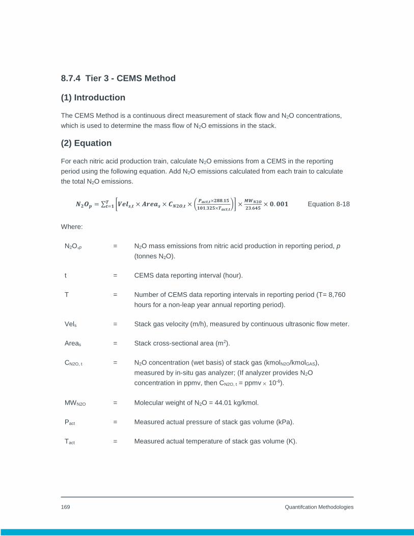
169 Quantifcation Methodologies
8.7.4 Tier 3 - CEMS Method
(1) Introduction
The CEMS Method is a continuous direct measurement of stack flow and N2O concentrations,
which is used to determine the mass flow of N2O emissions in the stack.
(2) Equation
For each nitric acid production train, calculate N2O emissions from a CEMS in the reporting
period using the following equation. Add N2O emissions calculated from each train to calculate
the total N2O emissions.
𝑵𝟐𝑶𝒑 = ∑ [𝑽𝒆𝒍𝒔,𝒕 × 𝑨𝒓𝒆𝒂𝒔 × 𝑪𝑵𝟐𝑶,𝒕 × (𝑷𝒂𝒄𝒕,𝒕×𝟐𝟖𝟖.𝟏𝟓
𝟏𝟎𝟏.𝟑𝟐𝟓×𝑻𝒂𝒄𝒕,𝒕)] ×
𝑴𝑾𝑵𝟐𝑶
𝟐𝟑.𝟔𝟒𝟓× 𝟎. 𝟎𝟎𝟏𝑻
𝒕=𝟏 Equation 8-18
Where:
N2O,p = N2O mass emissions from nitric acid production in reporting period, p
(tonnes N2O).
t = CEMS data reporting interval (hour).
T = Number of CEMS data reporting intervals in reporting period (T= 8,760
hours for a non-leap year annual reporting period).
Vels = Stack gas velocity (m/h), measured by continuous ultrasonic flow meter.
Areas = Stack cross-sectional area (m2).
CN2O, t = N2O concentration (wet basis) of stack gas (kmolN2O/kmolGAS),
measured by in-situ gas analyzer; (If analyzer provides N2O
concentration in ppmv, then CN2O, t = ppmv 10-6).
MWN2O = Molecular weight of N2O = 44.01 kg/kmol.
Pact = Measured actual pressure of stack gas volume (kPa).
Tact = Measured actual temperature of stack gas volume (K).
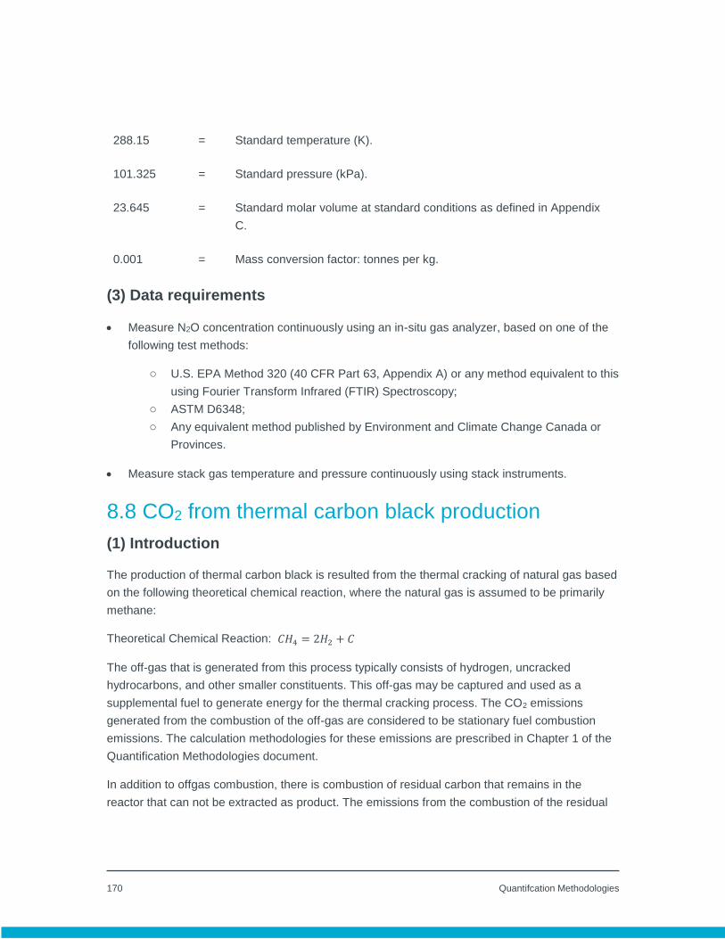
170 Quantifcation Methodologies
288.15 = Standard temperature (K).
101.325 = Standard pressure (kPa).
23.645 = Standard molar volume at standard conditions as defined in Appendix
C.
0.001 = Mass conversion factor: tonnes per kg.
(3) Data requirements
Measure N2O concentration continuously using an in-situ gas analyzer, based on one of the
following test methods:
o U.S. EPA Method 320 (40 CFR Part 63, Appendix A) or any method equivalent to this
using Fourier Transform Infrared (FTIR) Spectroscopy;
o ASTM D6348;
o Any equivalent method published by Environment and Climate Change Canada or
Provinces.
Measure stack gas temperature and pressure continuously using stack instruments.
8.8 CO2 from thermal carbon black production
(1) Introduction
The production of thermal carbon black is resulted from the thermal cracking of natural gas based
on the following theoretical chemical reaction, where the natural gas is assumed to be primarily
methane:
Theoretical Chemical Reaction: 𝐶𝐻4 = 2𝐻2 + 𝐶
The off-gas that is generated from this process typically consists of hydrogen, uncracked
hydrocarbons, and other smaller constituents. This off-gas may be captured and used as a
supplemental fuel to generate energy for the thermal cracking process. The CO2 emissions
generated from the combustion of the off-gas are considered to be stationary fuel combustion
emissions. The calculation methodologies for these emissions are prescribed in Chapter 1 of the
Quantification Methodologies document.
In addition to offgas combustion, there is combustion of residual carbon that remains in the
reactor that can not be extracted as product. The emissions from the combustion of the residual

171 Quantifcation Methodologies
carbon is considered to be IP as the combustion is unavoidable in the chemical production of
carbon black.
(2) Equations
The CO2 emissions from the combustion of the residual carbon are determined using Equation 8-
19. Equation 8-19a provides the equation to calculate the mass of carbon in the gaseous
feedstock and offgas.
𝑪𝑶𝟐,𝒑 = (𝒎𝑪,𝑭𝒆𝒆𝒅,𝒑 − 𝒎𝑪,𝑷𝒓𝒐𝒅𝒖𝒄𝒕,𝒑 − 𝒎𝑪,𝑶𝒇𝒇𝒈𝒂𝒔,𝒑) × 𝟑. 𝟔𝟔𝟒 Equation 8-19
Where:
CO2,p = CO2 mass emissions from the combustion of residual carbon in the
thermal carbon black production process during the reporting period, p
(tonnes CO2).
mC, Feed, p = Mass of carbon in the feedstock consumed in the reporting period, p
(tonnes C).
mC, Product,p = Mass of carbon in the product produced in the reporting period, p
(tonnes C).
mC, Offgas,p = Mass of carbon in the offgas consumed in the reporting period, p
(tonnes C).
3.664 = Ratio of molecular weights, CO2 to carbon.
𝒎𝑪,𝑭𝒆𝒆𝒅,𝒑𝒐𝒓 𝒎𝑪,𝑶𝒇𝒇𝒈𝒂𝒔,𝒑 = 𝝊𝒇𝒖𝒆𝒍(𝒈𝒂𝒔) × 𝑪𝑪𝒈𝒂𝒔,𝒑 × 𝟎. 𝟎𝟎𝟏 Equation 8-19a
Where:
mC,Feed,p or
mC,Offgas,p
= Mass of carbon in the gaseous feedstock or offgas used during the
reporting period, p (tonnes C).
νfuel (gas),p = Volume of the gaseous feedstock or offgas (m3) during the reporting
period, p, at standard conditions as defined in Appendix C.
CCgas,p = Weighted average carbon content of the gaseous feedstock or offgas
during the reporting period p, calculated in accordance with Chapter 17
172 Quantifcation Methodologies
and Appendix C. CCp is in units of kilogram of carbon per standard
cubic metre of gaseous fuel (kg C/m3).
0.001 = Mass conversion factor (t/kg).
(3) Data requirements
Facilities must ensure that the proper units of feedstock and offgas consumption and carbon
content are applied in Equation 8-19a.
Volume measurements must be adjusted to standard conditions as defined in Appendix C.
Mass of carbon in the product must be based on the facility's production accounting methods
used for the sale of product.

173 Quantifcation Methodologies
12.0 Quantification of Imports
12.1 Introduction
Imports are considered to be useful thermal energy, electricity and/or hydrogen that are brought
into the facility from another facility for consumption in production activities and/or facility
operations. Imports do not include quantities of thermal energy, electricity, and/or hydrogen that
are generated and consumed within the facility boundaries. Generation and export of these
parameters are quantified in a similar manner but are reported as a product, as described in
Chapter 13.
There is considerable variation in the consumption of imported and onsite generated electricity,
heat, and hydrogen in Alberta facilities, leading to variation in their direct emissions despite
otherwise comparable activity. Data on these imports allows these differences to be taken into
account when facility performance is compared over time, and across facilities. While other
imports also play a role in facility emissions variations, electricity, heat, and hydrogen imports
explain many significant emissions performance differences observed. The quantification of these
imports should be supported by documents such as invoices or third party documentation,
whenever possible, because they represent the shared position of both parties (producer and
importer) involved in these imports.
The reporting of imported quantities should be consistent with the overall facility boundaries used
for emissions and production reporting. For example, the inclusion of camps, roads, and
construction equipment must be consistent with facility boundary definitions.
12.2 Imported Useful Thermal Energy
Imported useful thermal energy refers to energy in any form transferred from a facility producing
industrial heat to another facility or residual thermal energy returning to a facility producing
industrial heat from a regulated facility or registered offset project, including heat transfer fluids,
steam, and hot water. Imported useful thermal energy is to be reported based on third party
invoices of total heat imported, if available. If third party invoices of total heat imported are not
available then total heat imported is to be calculated in accordance to Chapter 13.11.
The total heat imported is to be reported as follows:
Heatimported = Amount of useful thermal energy imported to the facility, reported in GJ.
174 Quantifcation Methodologies
12.3 Imported Electricity
Imported electricity refers to electricity generated outside the facility and delivered to the facility
from the grid or directly from electricity suppliers. Imported electricity is to be reported based on
third party invoices of total imported electricity if available. If third party invoices of imported
electricity are not available then total imported electricity is to be calculated in accordance to
Chapter 13.6.
The total electricity imported is to be reported as follows:
Eimported = Amount of electricity imported to the facility in MWh.
12.4 Imported Hydrogen
Imported hydrogen refers to hydrogen manufactured outside the facility and delivered to the
facility. Imported hydrogen is to be reported where hydrogen is greater than 5% of the gas stream
by volume. Imported hydrogen is to be reported based on third party invoices of total imported
hydrogen if available. If third party invoices of imported hydrogen are not available then total
imported hydrogen is to be calculated in accordance to Chapter 13.10.
The hydrogen imported is to be reported as follows:
Himported = Amount of imported hydrogen in tonnes.
As the imported hydrogen stream may contain other constituents (i.e. hydrocarbons, etc.), only
the mass of the hydrogen component is reported.
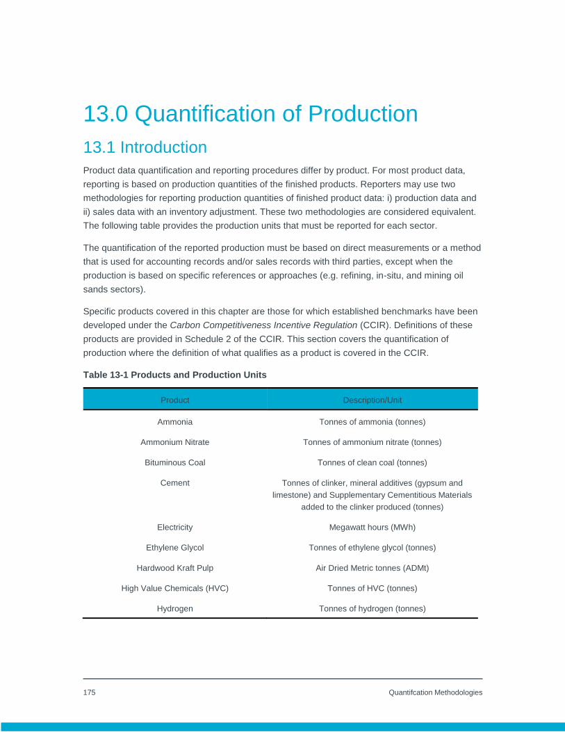
175 Quantifcation Methodologies
13.0 Quantification of Production
13.1 Introduction
Product data quantification and reporting procedures differ by product. For most product data,
reporting is based on production quantities of the finished products. Reporters may use two
methodologies for reporting production quantities of finished product data: i) production data and
ii) sales data with an inventory adjustment. These two methodologies are considered equivalent.
The following table provides the production units that must be reported for each sector.
The quantification of the reported production must be based on direct measurements or a method
that is used for accounting records and/or sales records with third parties, except when the
production is based on specific references or approaches (e.g. refining, in-situ, and mining oil
sands sectors).
Specific products covered in this chapter are those for which established benchmarks have been
developed under the Carbon Competitiveness Incentive Regulation (CCIR). Definitions of these
products are provided in Schedule 2 of the CCIR. This section covers the quantification of
production where the definition of what qualifies as a product is covered in the CCIR.
Table 13-1 Products and Production Units
Product Description/Unit
Ammonia Tonnes of ammonia (tonnes)
Ammonium Nitrate Tonnes of ammonium nitrate (tonnes)
Bituminous Coal Tonnes of clean coal (tonnes)
Cement Tonnes of clinker, mineral additives (gypsum and
limestone) and Supplementary Cementitious Materials
added to the clinker produced (tonnes)
Electricity Megawatt hours (MWh)
Ethylene Glycol Tonnes of ethylene glycol (tonnes)
Hardwood Kraft Pulp Air Dried Metric tonnes (ADMt)
High Value Chemicals (HVC) Tonnes of HVC (tonnes)
Hydrogen Tonnes of hydrogen (tonnes)
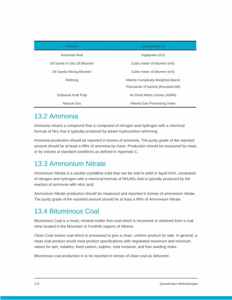
176 Quantifcation Methodologies
Product Description/Unit
Industrial Heat Gigajoules (GJ)
Oil Sands In Situ Oil Bitumen Cubic meter of bitumen (m3)
Oil Sands Mining Bitumen Cubic meter of bitumen (m3)
Refining Alberta Complexity-Weighted Barrel
Thousands of barrels (thousand bbl)
Softwood Kraft Pulp Air Dried Metric tonnes (ADMt)
Natural Gas Alberta Gas Processing Index
13.2 Ammonia
Ammonia means a compound that is composed of nitrogen and hydrogen with a chemical
formula of NH3 that is typically produced by steam hydrocarbon reforming.
Ammonia production should be reported in tonnes of ammonia. The purity grade of the reported
amount should be at least a 99% of ammonia by mass. Production should be measured by mass
or by volume at standard conditions as defined in Appendix C.
13.3 Ammonium Nitrate
Ammonium Nitrate is a soluble crystalline solid that can be sold in solid or liquid form, composed
of nitrogen and hydrogen with a chemical formula of NH4NO3 that is typically produced by the
reaction of ammonia with nitric acid.
Ammonium Nitrate production should be measured and reported in tonnes of ammonium nitrate.
The purity grade of the reported amount should be at least a 99% of Ammonium Nitrate.
13.4 Bituminous Coal
Bituminous Coal is a moist, mineral-matter free coal which is recovered or obtained from a coal
mine located in the Mountain or Foothills regions of Alberta.
Clean Coal means coal which is processed to give a clean, uniform product for sale. In general, a
clean coal product would meet product specifications with negotiated maximum and minimum
values for ash, volatiles, fixed carbon, sulphur, total moisture, and free swelling index.
Bituminous coal production is to be reported in tonnes of clean coal as delivered.

177 Quantifcation Methodologies
13.5 Cement
Cement is a fine powered material that consists of a mixture of clinker, gypsum, limestone, and
supplementary cementitious materials.
Cement production shall be measured and reported in tonnes after final blending. Cement
production is the total mass of clinker produced in tonnes, including mineral and other additives
(gypsum, limestone and supplementary cementitious materials).
13.6 Electricity
Electricity means electricity that is exported from the facility. Report electricity production as the
total electricity either sold to the end user directly or transmitted to the Alberta Electric System
Operator (AESO) controlled grid or an Industrial System (ISD). Electricity transactions (the
purchase, sale, import or export of electric power) must be quantified in accordance with the
AESO ISO definition for “metered energy” (ISO rule (2010-07-23)). Metered energy means the
quantity of electric energy transferred to a point of delivery or from a point of supply, in MWh,
reflected by the relevant metering equipment during a particular period of time.
13.7 Ethylene Glycol
As defined by CCIR.
13.8 Hardwood Kraft Pulp
Hardwood Kraft Pulp means wood pulp processed from hardwood species (typically Aspen,
Balsam Poplar, or White Birch) by a sulphate chemical process using cooking liquor. Annual
Hardwood Kraft Pulp production should be reported in ADMt (Air Dry Metric Tonnes - 10%
moisture by mass). Actual mass and moisture content should be measured by bale with
measured mass corrected back to a 10% moisture basis.
13.9 High Value Chemicals
As defined by CCIR.
13.10 Hydrogen
Hydrogen is a colorless elemental gas represented by the chemical formula H2 and is typically
produced by, steam methane reforming or hydrocarbon fractionation. Annual production of
hydrogen is based on direct measurements, accounting records or sales records with third

178 Quantifcation Methodologies
parties. As the hydrogen product stream may contain other constituents (i.e. hydrocarbons, etc.),
only the mass of the hydrogen component is reported.
13.11 Industrial Heat
Industrial heat is quantified as the total heat sold to a third party. Returned boiler feed water or
low pressure steam energy is not subtracted as this is to be separately reported as imported heat.
Annual production of Industrial Heat is based on sales records with third parties, or calculated in
accordance with Chapter 17, Tier 3 and Appendix C.
13.12 Oil Sands In Situ Bitumen
Oil sands in situ bitumen shall be reported consistent with the methodology required by Directive
042: Measurement, Accounting, and Reporting Plan (MARP) Requirement for Thermal Bitumen
Schemes and used for the Statistical Report 53 (ST-53) published by the Alberta Energy
Regulator in cubic meters.
13.13 Oil Sands Mining Bitumen
Oil sands mining bitumen shall be reported as the total mined crude bitumen production corrected
for inventory changes consistent with the methodology used for the Statistical Report 39 (ST-39)
published by the Alberta Energy Regulator in cubic meters.
13.14 Refining
13.14.1 Introduction
Refining means any manufacturing or industrial process that occurs at a refinery at which crude
oil or bitumen is processed or refined into a transportation fuel.
Complexity Weighted Barrel or CWB is a metric created by Solomon Associates to evaluate the
greenhouse gas efficiency of petroleum refineries and related processes. The Canadian version
of the methodology (CAN-CWB) is outlined in The CAN-CWB Methodology for Regulatory
Support: Public Report, January 2014 (CAN-CWB Methodology).
Alberta has adapted the CAN-CWB to the regulatory and technical requirements in the province
introducing the Alberta Complexity Weighed Barrel (AB-CWB) for use as production metric for the
refining sector in the province.
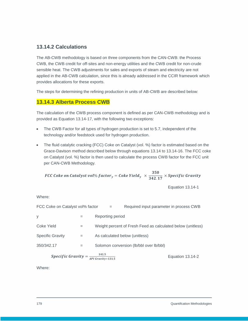
179 Quantifcation Methodologies
13.14.2 Calculations
The AB-CWB methodology is based on three components from the CAN-CWB: the Process
CWB, the CWB credit for off-sites and non-energy utilities and the CWB credit for non-crude
sensible heat. The CWB adjustments for sales and exports of steam and electricity are not
applied in the AB-CWB calculation, since this is already addressed in the CCIR framework which
provides allocations for these exports.
The steps for determining the refining production in units of AB-CWB are described below:
13.14.3 Alberta Process CWB
The calculation of the CWB process component is defined as per CAN-CWB methodology and is
provided as Equation 13.14-17, with the following two exceptions:
The CWB Factor for all types of hydrogen production is set to 5.7, independent of the
technology and/or feedstock used for hydrogen production.
The fluid catalytic cracking (FCC) Coke on Catalyst (vol. %) factor is estimated based on the
Grace-Davison method described below through equations 13.14 to 13.14-16. The FCC coke
on Catalyst (vol. %) factor is then used to calculate the process CWB factor for the FCC unit
per CAN-CWB Methodology.
𝑭𝑪𝑪 𝑪𝒐𝒌𝒆 𝒐𝒏 𝑪𝒂𝒕𝒂𝒍𝒚𝒔𝒕 𝒗𝒐𝒍% 𝒇𝒂𝒄𝒕𝒐𝒓𝒚 = 𝑪𝒐𝒌𝒆 𝒀𝒊𝒆𝒍𝒅𝒚 × 𝟑𝟓𝟎
𝟑𝟒𝟐. 𝟏𝟕 × 𝑺𝒑𝒆𝒄𝒊𝒇𝒊𝒄 𝑮𝒓𝒂𝒗𝒊𝒕𝒚
Equation 13.14-1
Where:
FCC Coke on Catalyst vol% factor = Required input parameter in process CWB
y = Reporting period
Coke Yield = Weight percent of Fresh Feed as calculated below (unitless)
Specific Gravity = As calculated below (unitless)
350/342.17 = Solomon conversion (lb/bbl over lb/bbl)
𝑺𝒑𝒆𝒄𝒊𝒇𝒊𝒄 𝑮𝒓𝒂𝒗𝒊𝒕𝒚 =𝟏𝟒𝟏.𝟓
𝑨𝑷𝑰 𝑮𝒓𝒂𝒗𝒊𝒕𝒚+𝟏𝟑𝟏.𝟓 Equation 13.14-2
Where:

180 Quantifcation Methodologies
API Gravity = As measured for combined FCC feed or aggregate of all
equivalent FCC feed streams
𝑪𝒐𝒌𝒆 𝒀𝒊𝒆𝒍𝒅 = 𝟏𝟎𝟎 ×𝑻𝒐𝒕𝒂𝒍 𝑪𝒐𝒌𝒆
𝑭𝑭 𝑹𝒂𝒕𝒆 Equation 13.14-3
Where:
Total Coke = As calculated below (lb/hr)
FF Rate = Fresh feed rate as calculated below (lb/hr)
𝑻𝒐𝒕𝒂𝒍 𝑪𝒐𝒌𝒆 = 𝑪𝒂𝒓𝒃𝒐𝒏 𝑹𝒆𝒈𝒆𝒏 𝑩𝒖𝒓𝒏 𝑹𝒂𝒕𝒆 + 𝑯𝒚𝒅𝒓𝒐𝒈𝒆𝒏 𝑹𝒆𝒈𝒆𝒏 𝑩𝒖𝒓𝒏 𝑹𝒂𝒕𝒆 +
𝑺𝒖𝒍𝒑𝒉𝒆𝒓 𝑹𝒆𝒈𝒆𝒏 𝑩𝒖𝒓𝒏 𝑹𝒂𝒕𝒆 + 𝑵𝒊𝒕𝒓𝒐𝒈𝒆𝒏 𝑹𝒆𝒈𝒆𝒏 𝑩𝒖𝒓𝒏 𝑹𝒂𝒕𝒆
Equation 13.14-4
Where:
Carbon Regen Burn Rate = As calculated below (lb/hr)
Hydrogen Regen Burn Rate = As calculated below (lb/hr)
Sulphur Regen Burn Rate = As calculated below (lb/hr)
Nitrogen Regen Burn Rate = As calculated below (lb/hr)
𝑪𝒂𝒓𝒃𝒐𝒏 𝑹𝒆𝒈𝒆𝒏 𝑩𝒖𝒓𝒏 𝑹𝒂𝒕𝒆 = 𝑴𝒐𝒍𝒆𝒄𝒖𝒍𝒂𝒓 𝑾𝒕 𝑪 ∗ (𝑪𝑶 𝒓𝒂𝒕𝒆 𝒊𝒏 𝒇𝒍𝒖𝒆 𝒈𝒂𝒔 +
𝑪𝑶𝟐 𝒓𝒂𝒕𝒆 𝒊𝒏 𝒇𝒍𝒖𝒆 𝒈𝒂𝒔) Equation 13.14-5
Where:
Molecular Wt C = 12.0107
CO rate in flue gas = As calculated below as component rate (lb/hr)
CO2 rate in flue gas = As calculated below as component rate (lb/hr)
𝑯𝒚𝒅𝒓𝒐𝒈𝒆𝒏 𝑹𝒆𝒈𝒆𝒏 𝑩𝒖𝒓𝒏 𝑹𝒂𝒕𝒆 = 𝑴𝒐𝒍𝒆𝒄𝒖𝒍𝒂𝒓 𝑾𝒕 𝑯𝟐 ∗ 𝑯𝟐𝑶 𝒓𝒂𝒕𝒆 𝒊𝒏 𝒇𝒍𝒖𝒆 𝒈𝒂𝒔
Equation 13.14-6
Where:
Molecular Wt H2 = 2.01588
H20 rate in flue gas = As calculated below (lb-mole/hr)
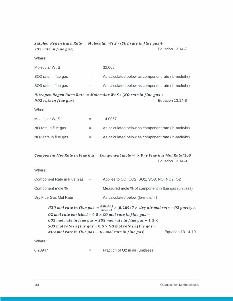
181 Quantifcation Methodologies
𝑺𝒖𝒍𝒑𝒉𝒆𝒓 𝑹𝒆𝒈𝒆𝒏 𝑩𝒖𝒓𝒏 𝑹𝒂𝒕𝒆 = 𝑴𝒐𝒍𝒆𝒄𝒖𝒍𝒂𝒓 𝑾𝒕 𝑺 ∗ (𝑺𝑶𝟐 𝒓𝒂𝒕𝒆 𝒊𝒏 𝒇𝒍𝒖𝒆 𝒈𝒂𝒔 +
𝑺𝑶𝟑 𝒓𝒂𝒕𝒆 𝒊𝒏 𝒇𝒍𝒖𝒆 𝒈𝒂𝒔) Equation 13.14-7
Where:
Molecular Wt S = 32.065
SO2 rate in flue gas = As calculated below as component rate (lb-mole/hr)
SO3 rate in flue gas = As calculated below as component rate (lb-mole/hr)
𝑵𝒊𝒕𝒓𝒐𝒈𝒆𝒏 𝑹𝒆𝒈𝒆𝒏 𝑩𝒖𝒓𝒏 𝑹𝒂𝒕𝒆 = 𝑴𝒐𝒍𝒆𝒄𝒖𝒍𝒂𝒓 𝑾𝒕 𝑺 ∗ (𝑵𝑶 𝒓𝒂𝒕𝒆 𝒊𝒏 𝒇𝒍𝒖𝒆 𝒈𝒂𝒔 +
𝑵𝑶𝟐 𝒓𝒂𝒕𝒆 𝒊𝒏 𝒇𝒍𝒖𝒆 𝒈𝒂𝒔) Equation 13.14-8
Where:
Molecular Wt S = 14.0067
NO rate in flue gas = As calculated below as component rate (lb-mole/hr)
NO2 rate in flue gas = As calculated below as component rate (lb-mole/hr)
𝑪𝒐𝒎𝒑𝒐𝒏𝒆𝒏𝒕 𝑴𝒐𝒍 𝑹𝒂𝒕𝒆 𝒊𝒏 𝑭𝒍𝒖𝒆 𝑮𝒂𝒔 = 𝑪𝒐𝒎𝒑𝒐𝒏𝒆𝒏𝒕 𝒎𝒐𝒍𝒆 % × 𝑫𝒓𝒚 𝑭𝒍𝒖𝒆 𝑮𝒂𝒔 𝑴𝒐𝒍 𝑹𝒂𝒕𝒆/𝟏𝟎𝟎
Equation 13.14-9
Where:
Component Rate in Flue Gas = Applies to CO, CO2, SO2, SO3, NO, NO2, O2
Component mole % = Measured mole % of component in flue gas (unitless)
Dry Flue Gas Mol Rate = As calculated below (lb-mole/hr)
𝑯𝟐𝑶 𝒎𝒐𝒍 𝒓𝒂𝒕𝒆 𝒊𝒏 𝒇𝒍𝒖𝒆 𝒈𝒂𝒔 =𝟐 𝒎𝒐𝒍𝒆 𝑯𝟐
𝒎𝒐𝒍𝒆 𝑶𝟐× [𝟎. 𝟐𝟎𝟗𝟒𝟕 × 𝒅𝒓𝒚 𝒂𝒊𝒓 𝒎𝒐𝒍 𝒓𝒂𝒕𝒆 + 𝑶𝟐 𝒑𝒖𝒓𝒊𝒕𝒚 ×
𝑶𝟐 𝒎𝒐𝒍 𝒓𝒂𝒕𝒆 𝒆𝒏𝒓𝒊𝒄𝒉𝒆𝒅 − 𝟎. 𝟓 × 𝑪𝑶 𝒎𝒐𝒍 𝒓𝒂𝒕𝒆 𝒊𝒏 𝒇𝒍𝒖𝒆 𝒈𝒂𝒔 −
𝑪𝑶𝟐 𝒎𝒐𝒍 𝒓𝒂𝒕𝒆 𝒊𝒏 𝒇𝒍𝒖𝒆 𝒈𝒂𝒔 − 𝑺𝑶𝟐 𝒎𝒐𝒍 𝒓𝒂𝒕𝒆 𝒊𝒏 𝒇𝒍𝒖𝒆 𝒈𝒂𝒔 − 𝟏. 𝟓 ×
𝑺𝑶𝟑 𝒎𝒐𝒍 𝒓𝒂𝒕𝒆 𝒊𝒏 𝒇𝒍𝒖𝒆 𝒈𝒂𝒔 − 𝟎. 𝟓 × 𝑵𝑶 𝒎𝒐𝒍 𝒓𝒂𝒕𝒆 𝒊𝒏 𝒇𝒍𝒖𝒆 𝒈𝒂𝒔 −
𝑵𝑶𝟐 𝒎𝒐𝒍 𝒓𝒂𝒕𝒆 𝒊𝒏 𝒇𝒍𝒖𝒆 𝒈𝒂𝒔 − 𝑶𝟐 𝒎𝒐𝒍 𝒓𝒂𝒕𝒆 𝒊𝒏 𝒇𝒍𝒖𝒆 𝒈𝒂𝒔] Equation 13.14-10
Where:
0.20947 = Fraction of O2 in air (unitless)
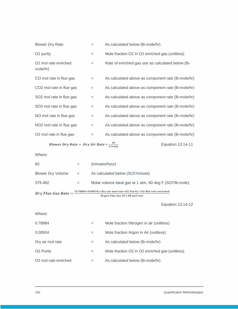
182 Quantifcation Methodologies
Blower Dry Rate = As calculated below (lb-mole/hr)
O2 purity = Mole fraction O2 in O2 enriched gas (unitless)
O2 mol rate enriched = Rate of enriched gas use as calculated below (lb-
mole/hr)
CO mol rate in flue gas = As calculated above as component rate (lb-mole/hr)
CO2 mol rate in flue gas = As calculated above as component rate (lb-mole/hr)
SO2 mol rate in flue gas = As calculated above as component rate (lb-mole/hr)
SO3 mol rate in flue gas = As calculated above as component rate (lb-mole/hr)
NO mol rate in flue gas = As calculated above as component rate (lb-mole/hr)
NO2 mol rate in flue gas = As calculated above as component rate (lb-mole/hr)
O2 mol rate in flue gas = As calculated above as component rate (lb-mole/hr)
𝑩𝒍𝒐𝒘𝒆𝒓 𝑫𝒓𝒚 𝑹𝒂𝒕𝒆 = 𝑫𝒓𝒚 𝑨𝒊𝒓 𝑹𝒂𝒕𝒆 ×𝟔𝟎
𝟑𝟕𝟗.𝟒𝟖𝟐 Equation 13.14-11
Where:
60 = (minutes/hour)
Blower Dry Volume = As calculated below (SCF/minute)
379.482 = Molar volume ideal gas at 1 atm, 60 deg F (SCF/lb-mole)
𝑫𝒓𝒚 𝑭𝒍𝒖𝒆 𝑮𝒂𝒔 𝑹𝒂𝒕𝒆 =(𝟎.𝟕𝟖𝟎𝟖𝟒+𝟎.𝟎𝟎𝟗𝟑𝟒)×𝑫𝒓𝒚 𝒂𝒊𝒓 𝒎𝒐𝒍 𝒓𝒂𝒕𝒆+𝑶𝟐 𝑷𝒖𝒓𝒊𝒕𝒚 ×𝑶𝟐 𝑴𝒐𝒍 𝒓𝒂𝒕𝒆 𝒆𝒏𝒓𝒊𝒄𝒉𝒆𝒅
𝑹𝒆𝒈𝒆𝒏 𝑭𝒍𝒖𝒆 𝑮𝒂𝒔 𝑵𝟐+𝑨𝑹 𝒎𝒐𝒍 𝒓𝒂𝒕𝒆
Equation 13.14-12
Where:
0.78984 = Mole fraction Nitrogen in air (unitless)
0.00934 = Mole fraction Argon in Air (unitless)
Dry air mol rate = As calculated below (lb-mole/hr)
O2 Purity = Mole fraction O2 in O2 enriched gas (unitless)
O2 mol rate enriched = As calculated below (lb-mole/hr)
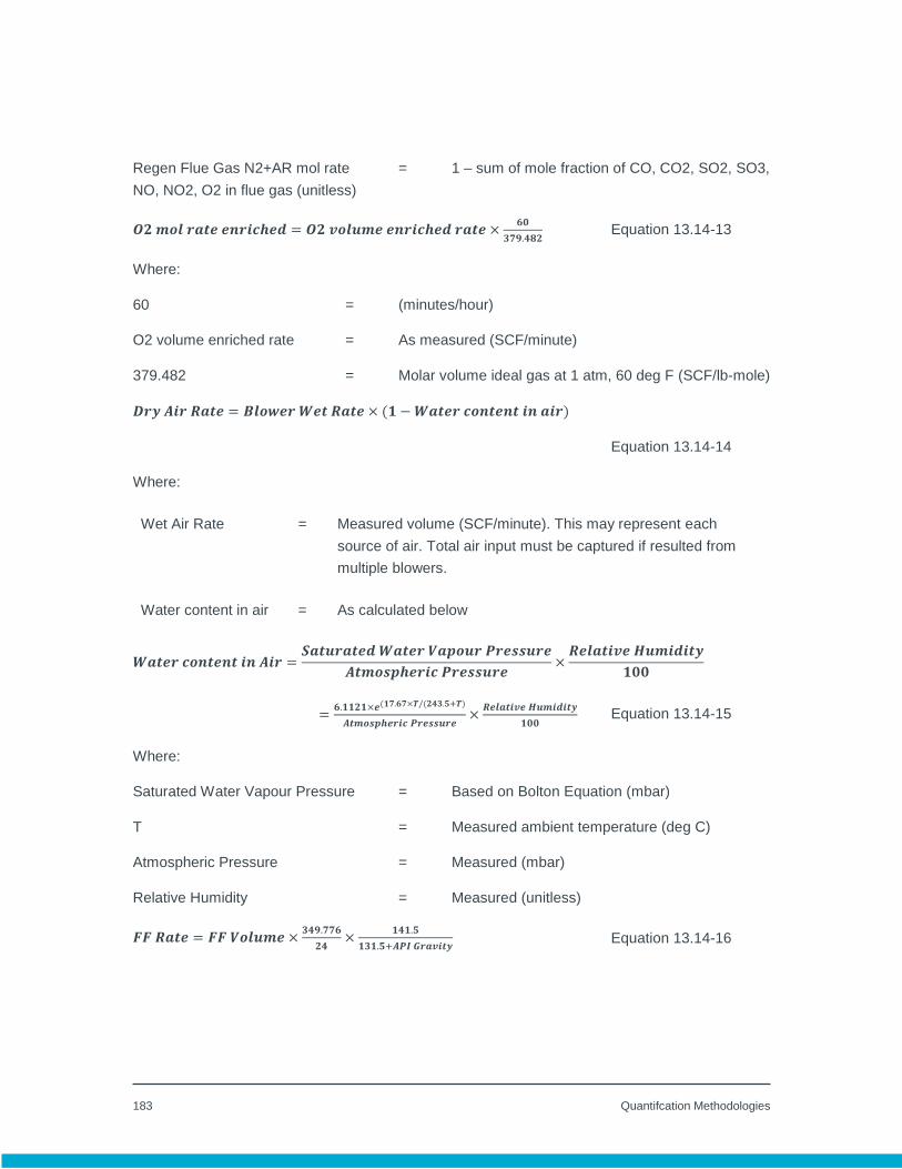
183 Quantifcation Methodologies
Regen Flue Gas N2+AR mol rate = 1 – sum of mole fraction of CO, CO2, SO2, SO3,
NO, NO2, O2 in flue gas (unitless)
𝑶𝟐 𝒎𝒐𝒍 𝒓𝒂𝒕𝒆 𝒆𝒏𝒓𝒊𝒄𝒉𝒆𝒅 = 𝑶𝟐 𝒗𝒐𝒍𝒖𝒎𝒆 𝒆𝒏𝒓𝒊𝒄𝒉𝒆𝒅 𝒓𝒂𝒕𝒆 ×𝟔𝟎
𝟑𝟕𝟗.𝟒𝟖𝟐 Equation 13.14-13
Where:
60 = (minutes/hour)
O2 volume enriched rate = As measured (SCF/minute)
379.482 = Molar volume ideal gas at 1 atm, 60 deg F (SCF/lb-mole)
𝑫𝒓𝒚 𝑨𝒊𝒓 𝑹𝒂𝒕𝒆 = 𝑩𝒍𝒐𝒘𝒆𝒓 𝑾𝒆𝒕 𝑹𝒂𝒕𝒆 × (𝟏 − 𝑾𝒂𝒕𝒆𝒓 𝒄𝒐𝒏𝒕𝒆𝒏𝒕 𝒊𝒏 𝒂𝒊𝒓)
Equation 13.14-14
Where:
Wet Air Rate = Measured volume (SCF/minute). This may represent each
source of air. Total air input must be captured if resulted from
multiple blowers.
Water content in air = As calculated below
𝑾𝒂𝒕𝒆𝒓 𝒄𝒐𝒏𝒕𝒆𝒏𝒕 𝒊𝒏 𝑨𝒊𝒓 =𝑺𝒂𝒕𝒖𝒓𝒂𝒕𝒆𝒅 𝑾𝒂𝒕𝒆𝒓 𝑽𝒂𝒑𝒐𝒖𝒓 𝑷𝒓𝒆𝒔𝒔𝒖𝒓𝒆
𝑨𝒕𝒎𝒐𝒔𝒑𝒉𝒆𝒓𝒊𝒄 𝑷𝒓𝒆𝒔𝒔𝒖𝒓𝒆×
𝑹𝒆𝒍𝒂𝒕𝒊𝒗𝒆 𝑯𝒖𝒎𝒊𝒅𝒊𝒕𝒚
𝟏𝟎𝟎
=𝟔.𝟏𝟏𝟐𝟏×𝒆(𝟏𝟕.𝟔𝟕×𝑻/(𝟐𝟒𝟑.𝟓+𝑻)
𝑨𝒕𝒎𝒐𝒔𝒑𝒉𝒆𝒓𝒊𝒄 𝑷𝒓𝒆𝒔𝒔𝒖𝒓𝒆×
𝑹𝒆𝒍𝒂𝒕𝒊𝒗𝒆 𝑯𝒖𝒎𝒊𝒅𝒊𝒕𝒚
𝟏𝟎𝟎 Equation 13.14-15
Where:
Saturated Water Vapour Pressure = Based on Bolton Equation (mbar)
T = Measured ambient temperature (deg C)
Atmospheric Pressure = Measured (mbar)
Relative Humidity = Measured (unitless)
𝑭𝑭 𝑹𝒂𝒕𝒆 = 𝑭𝑭 𝑽𝒐𝒍𝒖𝒎𝒆 ×𝟑𝟒𝟗.𝟕𝟕𝟔
𝟐𝟒×
𝟏𝟒𝟏.𝟓
𝟏𝟑𝟏.𝟓+𝑨𝑷𝑰 𝑮𝒓𝒂𝒗𝒊𝒕𝒚 Equation 13.14-16
184 Quantifcation Methodologies
Where:
FF Volume = Measured fresh feed volume (B/D)
349.776 = Water density at 60 F and 1 atm (lb/B)
API Gravity = Measured API Gravity of fresh feed (unitless)
24 = time conversion (hr/D)
𝑪𝑾𝑩𝒑𝒓𝒐 = ∑ 𝑫𝒂𝒊𝒍𝒚 𝑻𝒉𝒓𝒐𝒖𝒈𝒉𝒑𝒖𝒕 𝑩𝒂𝒓𝒓𝒆𝒍𝒖 × 𝑪𝑾𝑩 𝑭𝒂𝒄𝒕𝒐𝒓𝒖𝑼𝒖=𝟏 Equation 13.14-17
Where:
CWBpro [bbl/cd] = Alberta Process CWB as per CAN-CWB and section 13.14.3
u = Units in the refinery boundaries as per CAN-CWB
U = Total number of units in the refinery boundaries as per CAN-
CWB
Daily Throughput
Barrelu
= Throughput for unit u as defined in CAN-CWB in bbl/cd
CWB Factoru = CWB factor for unit u as defined in CAN-CWB except for
Hydrogen Production Unit.
13.14.4 Offsites and non-energy utilities CWB
The CWB credit for offsites and non-energy utilities (CWBoff) is calculated based on Process
CWB and Total Input Barrels. Total Input Barrels are defined as all raw material inputs to the
refinery less transfers of raw materials from the refinery. As per Solomon Associates raw
materials include:
Crude oil to be distilled and otherwise processed by the refinery.
Natural gas liquids and intermediate hydrocarbon materials that are processed by the
refinery, typically downstream from atmospheric crude distillation.
Blending components and additives that are blended by the refinery into its final products.
In determining Total Input Barrels all liquids should be measured in barrels at standard conditions
while gasses including hydrogen, natural gas, fuel gas, ethane, ethylene, and coke should be

185 Quantifcation Methodologies
expressed in Fuel Oil Equivalent Barrels where one Fuel Oil Equivalent Barrel is 6.05 million Btu
based on lower heating value.
13.14.5 Non-crude input barrels
The CWB credit for non-crude sensible heat (CWBnon) is calculated based on the non-crude input
barrels. Non-crude input barrels includes the total input raw material processed by the refinery
other than crude or other materials entering the atmospheric distillation unit. As per Solomon
Associates they potentially include:
Hydrogen and hydrogen-rich gas
Natural gas for hydrogen plant feed
Butane, isobutane, and mixed butanes
Natural gas liquids
Naphtha
Toluene
Light cycle oil
Sour kerosene
Sour diesel
Slop oil
Atmospheric gas oil
Coker gas oil
Heavy/vacuum gas oil
Vacuum residuum
Residual fuel oil
Atmospheric reduced crude oil and similar raw materials
All liquids should be measured in barrels at 60 F and 1 atm while gasses including hydrogen,
natural gas, fuel gas, ethane, ethylene and coke should be expressed in Fuel Oil Equivalent
Barrels where one Fuel Oil Equivalent Barrel is 6.05 million Btu based on lower heating value.

186 Quantifcation Methodologies
Blending raw materials which are not processed at the refinery are also not included. As per
Solomon Associates these may include the following types of material:
• Product additives
• Motor gasoline products and blendstocks, including but not limited to the following:
o − Ethanol, ETBE, MTBE, and other oxygenates
o − Butanes, pentanes, hexanes, isooctane, isooctane, mixed aromatics, benzene,
toluene, mixed xylenes, in addition to other specific hydrocarbons and hydrocarbon
mixtures that are suitable for gasoline blending
o − Alkylate, cat poly gasoline, coker gasoline, and reformate
o − Motor gasoline product that is purchased for blending by the refinery
• Kerosene products and blendstocks
• Diesel products and blendstocks including, but not limited to, the following:
o − Vegetable oil
o − Biodiesel
o − Diesel product for blending that is purchased for blending by the refinery
13.14.6 Refinery production measured in units of AB-CWB
The refinery production, measured in units of AB-CWB (AB-CWB in thousands of barrels per
calendar year) is calculated using equation 13.14-18 below:
𝑹𝒆𝒇𝒊𝒏𝒆𝒓𝒚 𝑷𝒓𝒐𝒅𝒖𝒄𝒕𝒊𝒐𝒏𝒚 =(𝑪𝑾𝑩𝒑𝒓𝒐+𝑪𝑾𝑩𝒐𝒇𝒇+𝑪𝑾𝑩𝒏𝒐𝒏)×𝑫𝒂𝒚𝒔
𝟏𝟎𝟎𝟎 Equation 13.14-18
Where:
Refinery Production y = AB-CWB Production of the refinery for year y, in thousand bbl/y
y = Reporting year
CWBpro [bbl/cd] = As per equation 13.14-17 for the reporting year
CWBoff [bbl/cd] = 0.327 × Total Input Barrels + 0.0085 × CWBpro
CWBnon [bbl/cd] = 0.44 × Non-Crude Input Barrels
Days = Days in the reporting year

187 Quantifcation Methodologies
The equation above includes the conversion from barrels per calendar day (as defined in the
CAN-CWB method) to thousands of barrels per calendar year, which is the unit used in the AB-
CWB.
13.15 Softwood Kraft Pulp
Softwood Kraft Pulp means wood pulp processed from softwood species (typically White Spruce,
Black Spruce, or Lodgepole Pine) by a sulphate chemical process using cooking liquor. Annual
Softwood Kraft Pulp production should be reported in ADMt (Air Dry Metric Tonnes - 10%
moisture by mass). Actual mass and moisture content should be measured by bale with
measured mass corrected back to a 10% moisture basis.
13.16 Alberta Gas Processing Index
For the natural gas processing sector, the benchmkark was developed based on a modular
approach. This approach accounts for differences in the configuration and complexity of Alberta's
natural gas processing facilities. The following section provides the quantification methodologies
for natural gas process facilities:
13.16.1 Glossary of Terms
Natural gas processing is a complex process that consists of operations involving separation of
impurities and various non-methane hydrocarbons and fluids from the raw natural gas to produce
a pipeline quality dry natural gas. The process is also used to recover natural gas liquids
(condensate, natural gasoline and liquefied petroleum gas) or other substances such as sulfur.
A ''Gas Processing Module'' is one or more grouped operations in the gas processing facility
that can be defined and separated from others.
Spec Product (SP) means ethane, propane, butanes or pentanes plus that have been processed
(fractionated) to a condition where they meet purchaser specifications for product quality. For
condensate (reported in Petrinex as PROC C5-SP), also includes condensate production that is
not further processed at the gas plant.
Petrinex is Canada’s upstream, midstream and downstream petroleum industry tool used for
reporting information required for the assessment, levy, and collection of crown royalties for the
provinces of Alberta and Saskatchewan.
Sulphur is an element produced as a by-product from the sour gas processing. It can be
extracted and/or stored in a prill, slate, block, or molten form.

188 Quantifcation Methodologies
Natural Gas Processing products in this document are defined by Oil And Gas Conservation Act
(2017), Province Of Alberta, such as:
Ethane (C2) means a mixture mainly of ethane that ordinarily may contain some methane or
propane
Propane (C3) means a mixture mainly of propane that ordinarily may contain some ethane or
butanes
Butanes (C4) means a mixture mainly of butanes that ordinarily may contain some propane
or pentanes plus
Natural Gas Liquid (NGL) means propane, butanes or pentanes plus, or a combination of
them, obtained from the processing of raw gas or condensate;
Pentanes plus (C5+) means a mixture mainly of pentanes and heavier hydrocarbons that
ordinarily may contain some
Condensate means a mixture mainly of pentanes and heavier hydrocarbons that may be
contaminated with sulphur compounds, that is recovered or is recoverable at a well from an
underground reservoir and may be gaseous in its virgin reservoir state but is liquid at the
conditions under which its volume is measured or estimated.
13.16.2 Unit Modules Description
Inlet Gas Compression
Inlet gas compression is a process that involves pressurizing/compressing inlet natural gas when
gas processing at the facility requires pressure higher than the pressure in the delivering pipeline.
The inlet gas throughput (E3m3) includes only the volume of the facility inlet gas that requires
compression before the gas enters the first processing module which operates at the facility’s
working pressure. Module throughputs include inlet gas volumes through both gas-fired and
electric-drive compressors.
Any re-compression that exists within a processing unit has been included in the benchmarking
for that particular unit and is not included in this module.
Dehydration
Dehydration of natural gas is a process that involves extraction of water vapor from the gas to a
specified maximum limit for residual water content. The most common dehydration processes
189 Quantifcation Methodologies
include, but not limited to, absorption with glycol and adsorption with dry desiccant. Glycol
dehydrating agents include diethylene glycol (DEG) and triethylene glycol (TEG). The most
common desiccants include activated alumina or a granular silica gel material.
The gas throughput volume (E3m3) reflects the total natural gas requiring dehydration. This
includes the volume of natural gas through a stand-alone glycol dehydration process and/or the
volume of natural gas processed through a molecular sieve dehydrator.
Gas Sweetening
Gas sweetening is a process involving removal of the CO2 and H2S from the raw gas to meet the
CO2 and H2S sales gas specifications. Gas sweetening agents may include, but are not limited
to primary, secondary, and tertiary amines and/or chemical compounds such as Selexol, Fluor,
Purisol, and Sulfinol. A “Merox” process may also be used to remove CO2 and H2S from the raw
gas stream.
The amine/gas sweetening throughput includes the total inlet gas volume in E3m3 through the
process.
Total Refrigeration
Refrigeration in natural gas treating is a process and/or series of processes that involve
separation of natural gas liquids (NGL) from the raw natural gas. Typical individual processes
include refrigeration, shallow cut, deep cut and lean oil systems. Refrigeration is also used to
meet the hydrocarbon dew point, as well as the water dew point specification for residue or sales
gas.
The refrigeration process primarily incorporates the two major methods: absorption and cryogenic
expander processes. An absorbing lean oil with high affinity for NGLs is used in the absorption
method. The turbo-expander and the Joule-Thomson expansion processes are used in the
cryogenic expander method.
The total gas throughput volume (E3m3) in the refrigeration module is determined based on the
configuration of refrigeration processes within a facility and is based on three scenarios, as
follows:
1. When only one refrigeration process exists within a facility, the total gas throughput volume
(E3m3) through this individual refrigeration processing module should be used.
2. When multiple refrigeration processes are run in series, the maximum throughput gas volume
(E3m3) through any individual refrigeration processing module should be used.
190 Quantifcation Methodologies
3. When the refrigeration processes are run in parallel, the total throughput gas volume (E3m3)
must be calculated based on the sum of throughput for each individual refrigeration
processing module operating in parallel.
Fractionation
Fractionation is a process that involves further separation of the NGLs removed from the natural
gas and/or NGLs brought onsite from a Third-Party contractor(s) for further
processing/fractionation. Fractionation is based on the different boiling points of different
hydrocarbons in the NGL stream. The fractionation process is broken down into steps in the
following processing order:
1. Deethanizer - removal of spec product ethane (C2-SP);
2. Depropanizer – removal of spec product propane (C3-SP); and
3. Debutanizer – removal of spec product butanes (normal- and iso- C4-SP), leaving the
pentanes and heavier hydrocarbons in the spec product pentane (C5-SP) and/or NGL
streams.
Deethanizer, Depropanizer and Debutanizer are referred as the “Fractionation processing
module”.
The production from the fractionation module includes the total production of specification (SP)
ethane, propane, butane, and pentane products reported in Petrinex in m3 and converted to cubic
metres of oil equivalent (m3OE).
Only the portion of C5 plus that goes through the fractionation module, reported as FRAC in
Petrinex, should be included here.
When pipeline specification ethane is produced in a Deep Cut Refrigeration process or in the
Ethane Extraction processing module at a straddle plant, it should not be included in the
fractionation production.
The total fractionation production should include specification products from both: Gas
Processing (reported as PROC in Petrinex excluding PROC Pentane-SP) and Fractionation
Processing (reported as FRAC in Petrinex).
Stabilization
Condensate stabilization is a process that involves a separation of the very light hydrocarbon
gases, e.g. methane and ethane, from the heavier hydrocarbon components so that a vapor
phase is not produced upon flashing the liquid into atmospheric storage tanks. Stabilization of the
condensate/pentanes+ is usually accomplished through flash vaporization.

191 Quantifcation Methodologies
The production from the stabilization module includes the total production of Pentane-SP reported
in Petrinex as PROC Pentane-SP in m3 and converted to cubic metres of oil equivalent (m3OE).
This should not include C5-SP produced in the fractionation module that is reported in Petrinex as
FRAC C5-SP.
Sales Compression
Sales gas compression involves pressurizing/compressing pipeline specification sales natural gas
to a pressure required for the natural gas transmission and distribution system.
The sales gas throughput (E3m3) includes only the volume of the sales gas leaving the facility
where the processing module operating pressure requires further compression prior to delivery to
the natural gas transmission and distribution system.
Any re-compression that exists within a processing unit has been included in the benchmarking
for that particular unit and is not included in this module.
Module throughputs include sales gas volume delivered to a natural gas transmission line through
both gas-fired and electric-drive compressors.
Sulphur Plant
Sulphur recovery is a process of recovering elemental sulfur from acid gas streams containing
hydrogen sulfide.
Hydrogen sulfide is a by-product of the sour natural gas processing. The “Claus Process” is the
most common method used is the recovery of elemental sulfur. The “Claus” technology consists
of a thermal stage (combustion chamber, waste heat boiler) and two or three catalytic reaction
stages (reheater, reactor and condenser). The sulfur produced in the thermal stage is condensed
in the waste heat boiler or the condenser. The remaining un-combusted hydrogen sulfide
undergoes the “Claus” catalytic reaction to form elemental sulfur. Alumina or titanium dioxide are
the most commonly used catalysts.
The sulphur plant production includes the sulphur production reported in Petrinex in tonnes of
sulphur.
Ethane Extraction
Ethane extraction is a process of removing ethane (including natural gas liquids) from marketable
natural gas. Facilities that utilize this process are also referred as straddle plants.

192 Quantifcation Methodologies
The most common ethane extraction process is a cryogenic process. The cryogenic process
consists of lowering the temperature of the gas stream, often with the use of a turbo expander
process. The natural gas stream is cooled by using external refrigerants, followed by an
expansion turbine, which rapidly expands the chilled gases. This causes the natural gas
temperature to drop significantly and rapidly, thus condensing ethane and other hydrocarbons.
Methane will remain in a gaseous form.
For straddle plants, the greenhouse gas emissions associated with dehydration, amine
sweetening and refrigeration processing are embedded within the ethane extraction plant so a
single ethane extraction processing module includes all three processes.
The ethane production includes the volume of ethane production (C2-SP) in E3m3 reported in
Petrinex and converted to cubic metres of oil equivalent (m3OE).
Acid Gas Injection
Acid gas injection is a process of injecting or disposing of the acid gas stream into a deep
geological formation. The two following steps are associated with the acid gas injection process,
after sulfur and carbon dioxide compounds are removed from the acid gas through an amine gas
treatment process:
1. The gas is transported through pipelines to a suitable place where it can be injected; and
2. The gas is forced into an injection well.
The acid gas injection throughput includes the total injected volume of acid gas (E3m3) reported
in Petrinex or measured at the facility.
Cavern Storage
Cavern storage is the storage of liquid hydrocarbon products in depleted salt caverns. This does
not include the storage of processed natural gas. The process of “displacement” is used to move
the product in and out of the cavern. Displacement uses brine to force product out of the cavern.
Since the brine is heavier than the hydrocarbons and sits below the product in the cavern, brine
can be pumped into the cavern through a pipe close to the bottom of the cavern to force the
product out through a pipe at the top of the cavern. As product is injected into the cavern, the
brine is removed from the bottom of the cavern. To make the displacement system work, most of
storage facilities maintain a large brine pond on the surface to move product in and out of the
cavern. The volume of the brine pond usually equals that of the volume of the cavern.
The cavern storage production includes the total volume of all liquefied gas product(s), i.e.
ethane, propane, butane and associated mixtures reported in m3 injected into the cavern(s).
193 Quantifcation Methodologies
Note: At this time, due to the small sample size, cavern storage allocations will be assigned on a
per facility basis.
CO2 Plant
The CO2 plant refers to a process involving the removal of CO2 from the gas stream, including
CO2 purification and/or liquefaction. The cryogenic technology is the most common and efficient
technology used in this process.
The CO2 plant processing module throughput includes the total CO2 gas volume (E3m3)
produced through the CO2 removal process as measured by facility meters or scales.
Flaring, Venting, Fugitives, Other
The “Flaring, Venting, Fugitives, Other” module includes all GHG emissions sources that are not
used for the purpose of gas or liquids processing at a regulated facility.
This module includes, but is not limited to, flare and incinerator stacks, venting (other than
formation CO2), facility fugitive emissions, residue gas for straddle plants, diesel emergency
generators, fire water pumps and other minor (<100 tonnes CO2e) emission sources.
The “Flaring, Venting, Fugitives, Other” throughput is taken as the total annual facility production
reported in Petrinex, converted to m3OE.
To further illustrate the concept of the natural gas processing modules, refer to Appendix E for an
overview of the modules followed by some typical natural gas plant configurations.
Average module intensities represented by weighting factors for Alberta Gas Processing Index
are also provided in the Appendix.
13.16.3 Production and Throughput Quantification Methods
The intent of this guidance is to align, to the extent possible, the requirements of the
Quantification Methodologies for the Carbon Competitiveness Incentive Regulation and the
Specified Gas Reporting Regulation and the Alberta Energy Regulator’s Directive 007: Volumetric
and Infrastructure Requirements. Both documents require production and throughput to be
reported at standard temperature and pressure conditions of 288.15 K and 101.325 kPa. No new
production metering requirements apply for the 2018 compliance year. Methods used should be
documented in the facility’s Quantification Methodology Document.
Alberta Environment and Parks recognizes that quantification of modular throughputs and
production will require flexibility for 2019 as facilities adapt to the new reporting requirements with
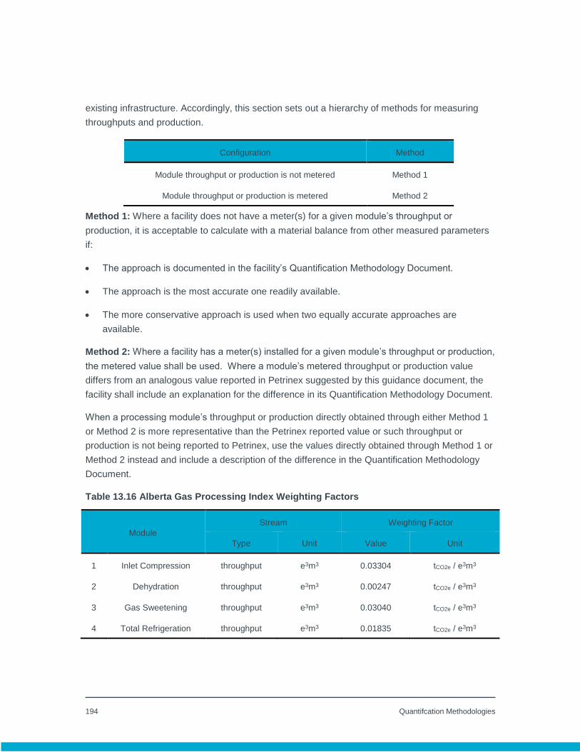
194 Quantifcation Methodologies
existing infrastructure. Accordingly, this section sets out a hierarchy of methods for measuring
throughputs and production.
Configuration Method
Module throughput or production is not metered Method 1
Module throughput or production is metered Method 2
Method 1: Where a facility does not have a meter(s) for a given module’s throughput or
production, it is acceptable to calculate with a material balance from other measured parameters
if:
The approach is documented in the facility’s Quantification Methodology Document.
The approach is the most accurate one readily available.
The more conservative approach is used when two equally accurate approaches are
available.
Method 2: Where a facility has a meter(s) installed for a given module’s throughput or production,
the metered value shall be used. Where a module’s metered throughput or production value
differs from an analogous value reported in Petrinex suggested by this guidance document, the
facility shall include an explanation for the difference in its Quantification Methodology Document.
When a processing module’s throughput or production directly obtained through either Method 1
or Method 2 is more representative than the Petrinex reported value or such throughput or
production is not being reported to Petrinex, use the values directly obtained through Method 1 or
Method 2 instead and include a description of the difference in the Quantification Methodology
Document.
Table 13.16 Alberta Gas Processing Index Weighting Factors
Module
Stream Weighting Factor
Type Unit Value Unit
1 Inlet Compression throughput e3m3 0.03304 tCO2e / e3m3
2 Dehydration throughput e3m3 0.00247 tCO2e / e3m3
3 Gas Sweetening throughput e3m3 0.03040 tCO2e / e3m3
4 Total Refrigeration throughput e3m3 0.01835 tCO2e / e3m3
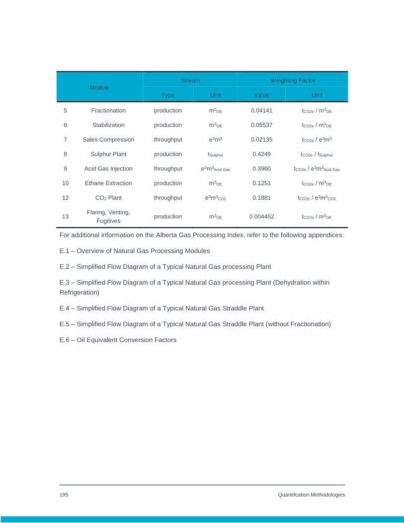
195 Quantifcation Methodologies
Module
Stream Weighting Factor
Type Unit Value Unit
5 Fractionation production m3OE 0.04141 tCO2e / m3
OE
6 Stabilization production m3OE 0.05537 tCO2e / m3
OE
7 Sales Compression throughput e3m3 0.02135 tCO2e / e3m3
8 Sulphur Plant production tSulphur 0.4249 tCO2e / tSulphur
9 Acid Gas Injection throughput e3m3Acid Gas 0.3960 tCO2e / e3m3
Acid Gas
10 Ethane Extraction production m3OE 0.1251 tCO2e / m3
OE
12 CO2 Plant throughput e3m3CO2 0.1881 tCO2e / e3m3
CO2
13 Flaring, Venting,
Fugitives production m3
OE 0.004452 tCO2e / m3OE
For additional information on the Alberta Gas Processing Index, refer to the following appendices:
E.1 – Overview of Natural Gas Processing Modules
E.2 – Simplified Flow Diagram of a Typical Natural Gas processing Plant
E.3 – Simplified Flow Diagram of a Typical Natural Gas processing Plant (Dehydration within
Refrigeration)
E.4 – Simplified Flow Diagram of a Typical Natural Gas Straddle Plant
E.5 – Simplified Flow Diagram of a Typical Natural Gas Straddle Plant (without Fractionation)
E.6 – Oil Equivalent Conversion Factors

196 Quantifcation Methodologies
14.0 Quantification Methods for Carbon Dioxide from Combustion of Biomass
14.1 Introduction
This chapter presents the methodologies for CO2 emissions from the combustion of biomass,
while CH4 and N2O emissions from the combustion of biomass are considered to be stationary
fuel combustion and are covered in Chapter 1.
14.2 Tier 1 - A fuel-specific default CO2 emission factor
(1) Introduction
This method is used for biomass fuels based on a default CO2 emission factor and the quantity of
fuel consumed. The quantity of biomass consumed may be in energy or physical unit basis, which
is measured by the facility using the methods prescribed in Chapter 17 and Appendix C. Biomass
consumption measured or provided in units of energy must be based on the HHV of the fuel.
Table 14-1 provides the emission factors for biomass fuels in mass of CO2 emitted per gigajoules
(GJ), tonnes or kilolitres (kl).
For facilities that have the HHV of the fuel, measured or supplied by the third party supplier,
Equation 14-1 is used to convert the volume or mass of the fuel to the energy of the fuel based on
the HHV and then multiplied by the appropriate energy based emission factor from Table 14-1 to
calculate the CO2 mass emissions. For facilities that have the quantity of fuel in energy basis,
Equation 14-1a can be used directly to calculate the CO2 mass emissions based on the
appropriate energy based emission factor from Table 14-1.
Facilities must use measured or supplied HHVs to determine the fuel consumption if this data is
available; however in cases where a facility is unable to obtain this information, a facility may
apply Equation 14-1a using the fuel quantity in mass/volume basis with the appropriate
mass/volume based emission factor from Table 14-1 to calculated the CO2 mass emissions.
Calculate the CO2 mass emissions for the reporting period for each type of biomass by
substituting a fuel-specific default CO2 emission, a measured or supplied HHV and the fuel
consumption for the reporting period into Equation 14-1 or Equation 14-1a.

197 Quantifcation Methodologies
(2) Equations
For a biomass fuel, use Equation 14-1 or Equation 14-1a to calculate the CO2 mass emissions for
the reporting period.
𝑪𝑶𝟐,𝒑 = 𝑭𝒖𝒆𝒍𝒑 × 𝑯𝑯𝑽 × 𝑬𝑭𝒆𝒏𝒆 Equation 14-1
𝑪𝑶𝟐,𝒑 = 𝑭𝒖𝒆𝒍𝒑 × 𝑬𝑭𝒗𝒐𝒍 𝒐𝒓 𝑬𝑭𝒆𝒏𝒆 Equation 14-1a
Where:
CO2,p = CO2 mass emissions for the biomass fuel for the reporting period, p (tonnes
CO2).
Fuelp = For Equation 14-1, the mass/volume of fuel combusted in tonnes or
kilolitres (tonnes or kl). For Equation 14-1a, energy units of fuel in
gigajoules or physical units of fuel in tonnes or kilolitres (GJ, tonnes, or kl).
Fuel quantities must be calculated in accordance with Chapter 17 and
Appendix C.
HHV = Measured or supplied higher heating value in gigajoules per tonne or
kilolitres (GJ/tonne or GJ/kl).
EFvol, EFene = Fuel-specific default CO2 emission factor, from Table 14-1 in tonnes of CO2
per energy units (GJ) or physical units (tonnes or kl).
(3) Data requirements
HHV is provided by the third party fuel supplier or measured by the facility in accordance with
Chapter 17 and Appendix C.
14.3 Tier 2 - Place marker.
14.4 Tier 3 - Measurement of fuel carbon content
(1) Introduction
Calculate the CO2 mass emissions from biomass combustion by using the measured fuel carbon
content using Equation 14-3a, Equation 14-3b, Equation 14-3c, or Equation 14-3d. For steam

198 Quantifcation Methodologies
generation from biomass combustion, CO2 mass emissions may be calculated using Equation 14-
3e.
(2) Equations
For gaseous biofuels, where fuel consumption is measured in units of volume (m3), use Equation
14-3a:
𝑪𝑶𝟐,𝒑 = 𝝊𝒇𝒖𝒆𝒍(𝒈𝒂𝒔),𝒑 × 𝑪𝑪𝒈𝒂𝒔,𝒑 × 𝟑. 𝟔𝟔𝟒 × 𝟎. 𝟎𝟎𝟏 Equation 14-3a
For gaseous biofuels, where fuel consumption is measured in units of energy (GJ), used Equation
14-3b:
𝑪𝑶𝟐,𝒑 =𝑬𝑵𝑬𝒇𝒖𝒆𝒍(𝒈𝒂𝒔)𝒑×𝑪𝑪𝒈𝒂𝒔,𝒑× 𝟑.𝟔𝟔𝟒×𝟎.𝟎𝟎𝟏
𝑯𝑯𝑽 Equation 14-3b
Where:
CO2,p = CO2 mass emissions for the gaseous biofuel combusted during the
reporting period, p (tonnes CO2).
νfuel(gas),p = Volume of fuel (m3) at standard conditions combusted during reporting
period, p, calculated in accordance with Chapter 17 and Appendix C.
ENEfuel(gas),p = Energy of fuel (GJ) at standard conditions combusted during reporting
period, p, calculated in accordance with Chapter 17 and Appendix C.
HHV = Weighted average higher heating value of biofuel (GJ/m3).
CCgas,p = Weighted average carbon content of the gaseous biofuel during the
reporting period p, calculated in accordance with Chapter 17 and Appendix
C. CCp is expressed in units of kilogram of carbon per standard cubic metre
of gaseous fuel (kg C/m3).
3.664 = Ratio of molecular weights, CO2 to carbon.
0.001 = Mass conversion factor (t/kg).
For liquid biofuels, where fuel consumption is measured in units of volume (kl), use Equation 14-
3c:
𝑪𝑶𝟐,𝒑 = 𝝊𝒇𝒖𝒆𝒍(𝒍𝒊𝒒),𝒑 × 𝑪𝑪𝒍𝒊𝒒,𝒑 × 𝟑. 𝟔𝟔𝟒 Equation 14-3c

199 Quantifcation Methodologies
Where:
CO2,p CO2 mass emissions for the liquid biofuels during the report period, p
(tonnes CO2).
ν fuel(liq),p Volume of liquid biofuel combusted during the reporting period p, calculated
in accordance with Chapter 17 and Appendix C (kl).
CCliq,p Weighted average carbon content of the liquid biofuel during the reporting
period
3.664 Ratio of molecular weights, CO2 to carbon.
For solid biomass fuels, where fuel consumption is measured in units of mass (tonnes), use
Equation 14-3d:
𝑪𝑶𝟐,𝒑 = 𝒎𝒇𝒖𝒆𝒍(𝒔𝒐𝒍),𝒑 × 𝑪𝑪𝒔𝒐𝒍,𝒑 × 𝟑. 𝟔𝟔𝟒 Equation 14-3d
Where:
CO2,p CO2 mass emissions for the biomass fuel during the report period, p
(tonnes CO2)
mfuel(sol),p Mass of biomass fuel combusted during the reporting period p, calculated in
accordance with Chapter 17 and Appendix C (tonnes).
CCsol,p Weighted average carbon content of the fuel during the reporting period p,
calculated in accordance with Chapter 17 and Appendix C. CCp is
expressed in units of tonnes of carbon per tonnes of solid fuel (tonnes
C/tonnes).
3.664 Ratio of molecular weights, CO2 to carbon.
For biomass combustion used to generate steam, use Equation 14-3e:
𝑪𝑶𝟐,𝒑 = 𝑺𝒕𝒆𝒂𝒎 × 𝑩 × 𝑬𝑭 Equation 14-3e
Where:

200 Quantifcation Methodologies
CO2,p CO2 mass emissions for the biomass fuel for the reporting period, p,
(tonnes CO2).
Steam Total steam generated by biomass fuel or biomass combustion during the
reporting year (tonnes steam), in GJ and calculated in accordance with
Chapter 17 and Appendix C.
B Ratio of the boiler’s design rated heat input capacity to its design rated
steam output capacity in GJ per GJ provided by the manufacturer or
calculated in
EF Measured emission factor for biomass solid fuel from a methodology
approved by the director, in tonnes of CO2 per GJ.
(3) Data requirements
No additional requirements are needed.
14.5 Tier 4 Continuous emissions monitoring systems
(1) Generality
Calculate the CO2 mass emissions for the reporting period from all fuels combusted in a unit, by
using data from CEMS as specified in (a) though (g). This methodology requires a CO2 monitor
and a flow monitoring subsystem, except as otherwise provided in paragraph (c). CEMS shall use
methodologies in accordance with reference [8] in Appendix A or by other document that
supersedes it.
(a) For a facility that operates CEMS in response to federal, provincial or local regulation (i.e.
required by the facility's Alberta Energy Regulator (AER) or Environmental Protection and
Enhancement Act (EPEA) approval), use CO2 or oxygen (O2) concentrations and flue gas
flow measurements to determine hourly CO2 mass emissions using methodologies provided
by the applicable regulatory requirements (i.e. facility's AER or EPEA approval) or in
accordance with reference [8] in Appendix A.
(b) Report CO2 emissions for the reporting period in tonnes based on the sum of hourly CO2
mass emissions over the reporting period.
(c) An O2 concentration monitor may be used in lieu of a CO2 concentration monitor in a CEMS
install before January 1, 2012, to determine the hourly CO2 concentrations, if the effluent gas
stream monitored by the CEMS consists of combustion products, and if only the following
201 Quantifcation Methodologies
fuels are combusted in the unit: coal, petroleum coke, oil, natural gas, propane, butane, wood
bark, or wood residue.
(i) If the operator of a facility that combusts biomass fuels uses O2 concentrations to
calculate CO2 concentrations, annual source testing must demonstrate that the
calculated CO2 concentrations, when compared to measured CO2 concentrations, meet
the Relative Accuracy Test Audit (RATA) requirements in reference [8] in Appendix A or
Alberta CEMS Code.
(d) If both biomass and fossil fuels (including fuels that are partially biomass) are combusted
during the reporting period, determine the biogenic CO2 mass emissions separately, as
described in Section 14.4 (2).
(e) For any units using CEMS data, industrial process and stationary combustion CO2 emissions
must be provided separately. Determine the quantities of each type of fossil fuel and biomass
consumed during the reporting period, using the fuel sampling approach in Table 17.3 of
Chapter 17.
(f) If a facility subject to requirements for continuous monitoring of gaseous emissions chooses
to add devices to an existing CEMS for the purpose of measuring CO2 concentrations or flue
gas flow, select and operate the added devices using appropriate requirements in
accordance with reference [8] in Appendix A for the facility, as applicable in Alberta under the
Alberta CEMS Code.
(g) If a facility does not have a CEMS and chooses to add one in order to measure CO2
concentrations, select and operate the CEMS using the appropriate requirements in
accordance with reference [8] in Appendix A or equivalent requirements as applicable in
Alberta under the Alberta CEMS Code.
(2) CO2 emissions from combustion of mixture of biomass, or
biomass fuels and fossil fuels
Use the procedures in this section to estimate biogenic CO2 emissions from units that combust a
combination of biomass and fossil fuels, including combustion of waste-derived fuels that are
partially biomass.
(a) If a CEMS is not used to measure CO2 and the facility combusts biomass fuels that do not
include waste-derived fuels (e.g., municipal solid waste and tires), use Tier 1, 2 or 3, as
applicable, to calculate the biogenic CO2 mass emissions for the reporting period from the
combustion of biomass fuels. Determine the mass of biomass combusted using either
company records or, for premixed fuels that contain biomass and fossil fuels (e.g., mixtures
containing biodiesel), use the best available information to determine the mass of biomass
fuels and document the procedure.
202 Quantifcation Methodologies
(b) If a CEMS is used to measure CO2 (or O2 as a surrogate) and the facility combusts biomass
fuels that do not include waste-derived fuels, use Tier 1, 2 or 3, as appropriate in Chapter 1,
to calculate the CO2 mass emissions for the reporting period from the combustion of fossil
fuels. Calculate biomass fuel emissions by subtracting the fossil fuel-related emissions from
the total CO2 emissions determined from the CEMS based methodology.
(c) If combusted fuels or fuel mixtures contain a biomass fraction that is unknown or cannot be
documented (e.g., wood waste and tire-derived fuel, etc.), or biomass fuels with no CO2
emission factor provided in Table 14-1 use the following to estimate biogenic CO2 emissions:
(i) Tier 1, 2, 3 or 4 to calculate the total CO2 mass emissions for the reporting period, as
applicable.
(3) Determine the biogenic portion of the CO2 emissions using ASTM D6866-16 “Standard
Test Methods for Determining the Biobased Content of Solid, Liquid, and Gaseous
Samples Using Radiocarbon Analysis”. This procedure is not required for fuels containing
less than 5% biomass by weight or for waste-derived fuels that are less than 30% by
weight of total fuels combusted in the year for which emissions are being reported,
except, if a facility wishes to report a biomass fuel fraction of CO2 emissions.
(4) Conduct analysis of representative fuel or exhaust gas samples at least every three
months, using ASTM D6866-16. Collect the exhaust gas samples over a minimum of 24
consecutive hours following the standard practice specified by ASTM D7459-08(2016)
“Standard Practice for Collection of Integrated Samples for the Speciation of Biomass
(Biogenic) and Fossil-Derived Carbon Dioxide Emitted from Stationary Emissions
Sources.”
(5) Allocate total CO2 emissions between biomass fuel emissions and non-biomass fuel
emissions using the average proportions of the samples analyzed annually for which
emissions are being reported.
(6) If there is a common fuel source for multiple units at the facility, ASTM D6866-16 analysis
may be conducted for only one of the unit sharing the common fuel source.
(d) If Equation 14-1 or 14-1a is selected to calculate the biogenic mass emissions for the
reporting period for wood, wood waste, or other solid biomass-derived fuel, Equation 14-4
may be used to quantify biogenic fuel consumption, provided that all of the required input
parameters are accurately quantified according to Chapter 17 and Appendix C. Similar
equations and calculation methodologies based on steam generation and boiler efficiency
may be used, provided that they are documented.
𝑭𝒖𝒆𝒍𝒊 = [𝑯 ×𝑺𝒕𝒆𝒂𝒎]− (𝑯𝑰)𝒏𝒃×(𝑬𝒇𝒇)𝒏𝒃
(𝑯𝑯𝑽)𝒃𝒊𝒐× (𝑬𝒇𝒇)𝒃𝒊𝒐 Equation 14-4

203 Quantifcation Methodologies
Where:
Fueli = Quantity of biomass consumed during the measurement period i
(tonnes/year or tonnes/month, as applicable) calculated in accordance with
Section 17.
H = Average enthalpy increase of the boiler steam through the boiler for the
Steam = Total boiler steam production for the measurement period (tonne/month or
tonne/year, as applicable) calculated in accordance with Chapter 17.
(HI)nb = Heat input from co-fired fossil fuel and non-biomass-derived fuels for the
(HHV)bio = Default or measured higher heating value of the biomass fuel (GJ/tonne)
(Eff)bio = Efficiency of biomass-to-energy conversion for boiler, expressed as a
decimal fraction and calculated in accordance with Chapter 17.
(Eff)nb = Efficiency of fossil fuel and non-biomass derived fuel to energy conversion
for boiler, expressed as a decimal fraction.
(3) Data requirements
No additional data requirement are needed.
14.6 Emission Factors
Table 14-1 Default emission factors for biomass fuels
Biomass Fuel HHV
(GJ/kl)
CO2 Emission Factor
tonne/kl tonne/GJ
Reference
Ethanol 23.42 1.508 0.0644 ECCC Table 2-2
Biodiesel 35.16 2.472 0.0703 ECCC Table 2-2
HHV
(GJ/tonne)
tonne/tonne tonne/GJ Reference
Wood Fuel / Wood Waste 18.0 0.840 0.0467 ECCC Table 2-3
Spent Pulping Liquor 14.0 0.891 0.0636 ECCC Table 2-3
204 Quantifcation Methodologies
17.0 Measurement, Sampling, Analysis and Data Management Requirements
17.1 Introduction
The methodologies prescribed in this chapter are intended to be aligned with methods that are
prescribed under Environment and Climate Change Canada (ECCC) and other jurisdictions that
regulate greenhouse gas emissions such as British Columbia, Ontario, Quebec, and California.
Further, methodologies from organizations such as the Western Climate Initiative, Inc. (WCI),
United States Environmental Protection Agency (USEPA), and the Intergovernmental Panel on
Climate Change (IPCC) are referenced or adopted as appropriate for various activity types and
modified to meet the needs of Alberta sectors.
17.2 Fuel consumption
17.2.1 Fuel consumption measurement requirements
Facilities may determine fuel consumption on the basis of direct measurement, fuel purchase
records, or sales invoices measuring any stock change. Equation 17-1 is used to quantify fuel
consumption.
𝑭𝒖𝒆𝒍 = 𝑭𝒖𝒆𝒍𝒑 − 𝑭𝒖𝒆𝒍𝒔 + 𝑭𝒖𝒆𝒍𝒊𝒊 − 𝑭𝒖𝒆𝒍𝒆𝒊 Equation 17-1
Where:
Fuel = amount of fuel used by the facility in the reporting year
Fuelp = amount of fuel purchased in the reporting year
Fuels = amount of fuel sold in the reporting year
Fuelii = initial amount of fuel in the inventories
Fuelei = ending amount of fuel in the inventories
(a) Facilities may quantify liquid fuels consumed at the facility based on third party invoices for
the reporting period without accounting for the initial and ending fuel quantities in the
inventories for the reporting period provided that:

205 Quantifcation Methodologies
(i) the liquid fuels are stored in a storage tank with a volume of 120,000 litres or less; and
(ii) the method to calculate these emissions are consistent from year to year.
(b) For solid fuels such as coal and coke, the facility must use direct measurements taken at a
location in the fuel handling system that is representative of the fuel consumed for the
reporting period. Measurement devices such as a weightometer may be used for direct
measurements.
(c) For liquid fuels, the facility must use direct tank level measurements, volumetric or mass flow
meters, and/or third party invoices. Tank level measurements may be used in combination
with third party invoices to determine liquid fuel consumption.
(d) For gaseous fuels, the facility must used direct measurements such as gas flow metering
and/or third party invoices or custody metering that is representative of the fuel consumed for
the reporting period.
(e) Fuel that is used as feedstock in industrial processes involving chemical or physical reactions
other than combustion may utilize the same monitoring requirements as for fuel combustion.
This includes gaseous fuels (i.e. natural gas) that are used in steam methane reforming
processes.
(f) Fuel consumption may be estimated per the following:
(i) For Tier 1 classification, facilities may estimate fuel consumption from combustion
equipment or mobile equipment based on the methodology outlined in Section C.6 of
Appendix C.
(ii) For Tiers 2 and 3, Section C.6 of Appendix C can be used to estimate fuel use from
negligible sources; otherwise Equation 17-1 must be used.
(iii) For Tiers 2 and 3, Section C.7 of Appendix C can be used to allocate fuel use for
individual equipment if the total fuel use can be measured or quantified, but the fuel use
for individual equipment cannot.
(g) Fuel flow meters that measure mass flow rates may be used for liquid fuels, provided that the
fuel density is used to convert the readings to volumetric flow rates. The density shall be
measured at the same frequency as the carbon content, using ASTM D1298-99 (Reapproved
2005) “Standard Test Method for Density, Relative Density (Specific Gravity), API Gravity of
Crude Petroleum and Liquid Petroleum Products by Hydrometer Method.”, or an alternative
method that is appropriate based on a method published by a consensus-based standards
organization.
(h) Fuel that is used as feed in industrial processes involving chemical or physical reactions
other than combustion may utilize the same monitoring requirements as for fuel combustion.

206 Quantifcation Methodologies
This includes gaseous fuels (i.e. natural gas) that are used in steam methane reforming
processes.
17.2.2 Calibration
(a) All fuel oil and gas flow meters (except for gas billing meters) shall be calibrated prior to the
first year for which GHG emissions are reported under this rule, using calibration procedures
specified by the flow meter manufacturer. Fuel flow meters shall be recalibrated once every
three years, upon replacement of a previously calibrated meter or at the minimum frequency
specified by the manufacturer. For orifice, nozzle, and venturi flow meters, the calibration
shall consists of in-situ calibration of the differential pressure (delta-P), total pressure, and
temperature transmitters. For flow meters used for natural gas, the facility may follow the
requirements prescribed by Alberta Energy Regulator, Measurement Canada, or other
regulations or standards for electricity and gas, as applicable for the facility.
(b) Scales and other instruments used for measuring solid and liquid fuels or industrial
feedstocks shall be calibrated, at the lesser of, once a year or at the minimum frequency
specified by the manufacturer.
17.2.3 Fuel properties
(1) Density
(a) Facilities using Tiers 1 or 2 for CO2 emissions may use the default density values for fuel oil
provided in Table B-3 in Appendix B, in lieu of using the ASTM method in paragraph (d) of
Section 17.2.1.
(b) For Tier 3, the density shall be measured at the same frequency as the carbon content, using
ASTM D1298-99 (Reapproved 2005) “Standard Test Method for Density, Relative Density
(Specific Gravity), API Gravity of Crude Petroleum and Liquid Petroleum Products by
Hydrometer Method.”, or an alternative method that is appropriate based on a method
published by a consensus-based standards organization.
(2) Fuel heat content
Fuel heat content sampling and analysis shall be as follows:
(a) For fuel heat content monitoring of natural gas, the facilities may
(i) Follow the requirements prescribed by Alberta Energy Regulator, Measurement Canada,
or other regulations or standards for electricity and gas, as applicable for the facility;

207 Quantifcation Methodologies
(ii) Use on-line instrumentation that determines heating value accurate to within ±0.5 per
cent and if such instrumentation provides only low heat value, the facility shall convert the
value to HHV using Equation 17-2 in accordance with the following:
1. The conversion factor (CF) for LHV to HHV, shall be determined as a fuel-
specific average CF using the following:
(a) Concurrent LHV and HHV measurements determined by on-line instrumentation
or laboratory analysis as part of the monthly carbon content determination; or
(b) The HHV/LHV ratio obtained from the laboratory analysis of the monthly samples
𝑯𝑯𝑽 = 𝑳𝑯𝑽 × 𝑪𝑭 Equation 17-2
Where:
HHV = Fuel or fuel mixture higher heat value
LHV = Fuel or fuel mixture lower heat value
CF = Conversion factor
(b) For gases, use the most appropriate method published by a consensus-based standards
organization, if such a method exists or a method required by the facility's AER or EPEA
approval. Specific test procedures may include ASTM D1826 “Standard Test Method for
Calorific (Heating) Value of Gases in Natural Gas Range by Continuous Recording
Calorimeter”, ASTM D3588 “Standard Practice for Calculating Heat Value, Compressibility
Factor, and Relative Density of Gaseous Fuels”, or ASTM D4891-, GPA Standard 2261
“Analysis for Natural Gas and Similar Gaseous Mixtures by Gas Chromatography.”
(c) For middle distillates and oil, or liquid waste-derived fuels, use the most appropriate method
published by a consensus-based standards organization or a method required by the facility's
AER or EPEA approval. Specific test procedures may include ASTM D240 “Standard Test
Method for Heat of Combustion of Liquid Hydrocarbon Fuels by Bomb Calorimeter” or ASTM
D4809 “Standard Test Method for Heat of Combustion of Liquid Hydrocarbon Fuels by Bomb
Calorimeter (Precision Method).” If no appropriate method is published by a consensus-
based standards organization, use industry standard methods, noting where such methods
are used and what methods are used.
(d) For solid biomass-derived fuels, use the most appropriate method published by a consensus-
based standards organization or a method required by the facility's AER or EPEA approval.
Specific test procedures may include ASTM D5865 “Standard Test Method for Gross Calorific
Value of Coal and Coke.” If no appropriate method is published by a consensus-based
208 Quantifcation Methodologies
standards organization, use industry standard methods, noting where such methods are used
and what methods are used.
(e) For waste-derived fuels, use the most appropriate method published by a consensus-based
standards organization or a method required by the facility's AER or EPEA approval. Specific
test procedures may include ASTM D5865 and ASTM D5468 “Standard Test Method for
Gross Calorific and Ash Value of Waste Materials.”
(f) For black liquor, use Technical Association of the Pulp and Paper Industry (TAPPI) T684 om-
15 - Gross High Heating Value of Black Liquor or equivalent method.
17.2.4 Fuel carbon content monitoring requirements
The determination of fuel carbon content and either molecular weight or molar fraction for
gaseous fuels shall be based on the results of fuel sampling and analysis received from the fuel
supplier, online calibrated analyzers or determined by the operator, using an applicable analytical
method listed below. For carbon content monitoring of natural gas, the facility may follow the
requirements prescribed by Alberta Energy Regulator, Measurement Canada or other regulations
or standards for electricity and gas, as applicable for the facility.
Appendix B: Fuel Properties and Appendix C: General Calculation Instructions provide guidance
for the use of fuel properties and calculation of carbon content and carbon content uncertainties.
(1) Solid fuel
For coal and coke, solid biomass fuels, and waste-derived fuels, and any other solid fuel use the
most appropriate method published by a consensus-based standards organization or a method
required by the facility's AER or EPEA approval. Specific test procedures may include ASTM
5373 “Standard Test Methods for Instrumental Determination of Carbon, Hydrogen, and Nitrogen
in Laboratory Samples of Coal”. If no appropriate method is published by a consensus-based
standards organization, use industry standard methods, noting where such methods are used
and what methods are used. Operators of coal fired electricity generators are expected to apply
additional quality control procedures to ensure accuracy of measured fuel carbon content.
(2) Liquid fuel
For liquid fuels, use the most appropriate method published by a consensus-based standards
organization or a method required by the facility's AER or EPEA approval. Specific test
procedures may include the following ASTM methods: For petroleum-based liquid fuels and liquid
waste-derived fuels, use ASTM D5291 “Standard Test Methods for Instrumental Determination of
Carbon, Hydrogen, and Nitrogen in Petroleum Products and Lubricants,” ultimate analysis of oil
or computations based on ASTM D3238, and either ASTM D2502 “Standard Test Method for

209 Quantifcation Methodologies
Estimation of Mean Relative Molecular Mass of Petroleum Oils From Viscosity Measurements” or
ASTM D2503 “Standard Test Method for Relative Molecular Mass (Molecular Weight) of
Hydrocarbons by Thermoelectric Measurement of Vapor Pressure.” If no appropriate method is
published by a consensus-based standards organization, use industry standard methods, noting
where such methods are used and what methods are used.
(3) Gaseous fuel
For gaseous fuels, use the most appropriate method published by a consensus-based standards
organization or a method required by the facility's AER or EPEA approval. Specific test
procedures may include ASTM D1945 “Standard Test Method for Analysis of Natural Gas by Gas
Chromatography” or ASTM D1946 “Standard Practice for Analysis of Reformed Gas by Gas
Chromatography.” If no appropriate method is published by a consensus-based standards
organization, use industry standard methods, noting where such methods are used and what
methods are used.
17.3 Equipment, fuel and properties sampling frequency
17.3.1 Introduction
The facility is required to obtain fuel samples pursuant to this standard quantification method by
conducting fuel sampling or obtaining fuel sampling results from the fuel supplier in accordance
with the following rules:
(a) Fuel samples shall be taken at a location in the fuel handling system that provides a
representative sample of the fuel combusted or consumed.
(b) Fuel samples shall be obtained and analysis performed at the minimum frequencies
prescribed in Table 17-3.
(c) In the event that more than one sampling frequency criteria is applicable to a fuel type, the
higher sampling frequency shall be applied.
(d) If a facility is sampling at a higher frequency than prescribed in Table 17.3, the facility must
ensure that the analysis used is representative and unbiased.
(e) Facilities must apply the sampling frequencies prescribed in Table 17-3 for the quantification
of the fuel consumed where applicable.
(f) Samples shall be representative of the fuel chemical and physical characteristics immediately
prior to combustion.
(g) Fuel that is used as feed in industrial processes involving chemical or physical reactions
other than combustion may utilize the same monitoring requirements as for fuel combustion.

210 Quantifcation Methodologies
This includes gaseous fuels (i.e. natural gas) that are used in steam methane reforming
processes.
(h) In the event that more than one sampling frequency criteria is applicable to a fuel type, the
higher sampling frequency shall be applied.
Table 17-3 Summary of Minimum Required Sampling/Monitoring Frequency for Fuels or
Feed Gases
Type of Fuel Tier 1 Tier 2 Tier 3
Purchased gasoline, and
diesel,
No sampling required No sampling required No sampling required
Ethane, propane, and butane No sampling required No sampling required No sampling required
Fuel received by batches No sampling required Six times a year By shipment
Marketable natural gas
(including natural gas feed
used for industrial processes)
No sampling required Six times a year Monthly
Non-marketable liquid or
gaseous fuels such as purge
gas co-produced at an oil and
gas production or
petrochemical facility.
No sampling required Quarterly Monthly
Gases derived from biomass
and biogas
No sampling required Quarterly Quarterly
Refinery fuel gas
No sampling required Every two weeks Daily (online
instrumentation in place)
Weekly (online
instrumentation not in
place)
Feedgases which result in
industrial process emissions.
No sampling required Every two weeks Daily (online
instrumentation in place)
Weekly (online
instrumentation not in
place)
Coal / Coke No Sampling required Monthly Once for each new fuel
shipment or delivery.
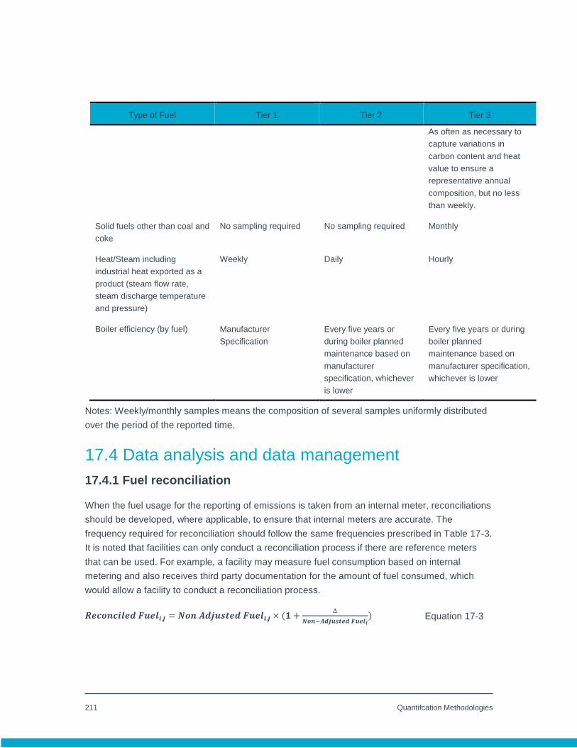
211 Quantifcation Methodologies
Type of Fuel Tier 1 Tier 2 Tier 3
As often as necessary to
capture variations in
carbon content and heat
value to ensure a
representative annual
composition, but no less
than weekly.
Solid fuels other than coal and
coke
No sampling required No sampling required Monthly
Heat/Steam including
industrial heat exported as a
product (steam flow rate,
steam discharge temperature
and pressure)
Weekly Daily Hourly
Boiler efficiency (by fuel) Manufacturer
Specification
Every five years or
during boiler planned
maintenance based on
manufacturer
specification, whichever
is lower
Every five years or during
boiler planned
maintenance based on
manufacturer specification,
whichever is lower
Notes: Weekly/monthly samples means the composition of several samples uniformly distributed
over the period of the reported time.
17.4 Data analysis and data management
17.4.1 Fuel reconciliation
When the fuel usage for the reporting of emissions is taken from an internal meter, reconciliations
should be developed, where applicable, to ensure that internal meters are accurate. The
frequency required for reconciliation should follow the same frequencies prescribed in Table 17-3.
It is noted that facilities can only conduct a reconciliation process if there are reference meters
that can be used. For example, a facility may measure fuel consumption based on internal
metering and also receives third party documentation for the amount of fuel consumed, which
would allow a facility to conduct a reconciliation process.
𝑹𝒆𝒄𝒐𝒏𝒄𝒊𝒍𝒆𝒅 𝑭𝒖𝒆𝒍𝒊,𝒋 = 𝑵𝒐𝒏 𝑨𝒅𝒋𝒖𝒔𝒕𝒆𝒅 𝑭𝒖𝒆𝒍𝒊,𝒋 × (𝟏 +Δ
𝑵𝒐𝒏−𝑨𝒅𝒋𝒖𝒔𝒕𝒆𝒅 𝑭𝒖𝒆𝒍𝒊) Equation 17-3
212 Quantifcation Methodologies
𝚫 = 𝑹𝒆𝒇𝒆𝒓𝒆𝒏𝒄𝒆 𝑭𝒖𝒆𝒍𝒊 − 𝑵𝒐𝒏 𝑨𝒅𝒋𝒖𝒔𝒕𝒆𝒅 𝑭𝒖𝒆𝒍𝒊 Equation 17-4
𝑵𝒐𝒏 𝑨𝒅𝒋𝒖𝒔𝒕𝒆𝒅 𝑭𝒖𝒆𝒍𝒊 = ∑ 𝑵𝒐𝒏 𝑨𝒅𝒋𝒖𝒔𝒕𝒆𝒅 𝑭𝒖𝒆𝒍𝒊,𝒋𝒏𝒋=𝟏 Equation 17-5
Where:
Reconciled
Fueli, j
= Amount of reconciled stream j for the fuel i at standard conditions as
defined in Appendix C.
Non-Adjusted
Fueli
= Amount of unreconciled fuel i at standard conditions. These are
Non-Adjusted
Fueli, j
= Amount of unreconciled stream j for the fuel i in standard conditions as
defined in Appendix C.
Reference
Fueli
= Reference amount of fuel i used for reconciliation of the
Δ = Amount of fuel to be adjusted.
17.4.2 Procedures for estimating missing data
The following method for estimating missing data was adapted from ECCC's Canada's
Greenhouse Gas Quantification Requirements, December 2017.
Whenever a quality-assured value of a required parameter for emissions calculations is
unavailable (e.g., if a CEMS malfunctions or fuel meter during unit operation or if a required fuel
sample is not taken), a substitute data value for the missing parameter shall be used in the
calculations.
(a) Whenever analytical data relating to sampling is unavailable, the facility shall, using the
methods prescribed in Section 17.3, re-analyze the original sample, a backup sample or a
replacement sample for the same measurement and sampling period; if this is not physically
possible, the operator should follow the missing data approach.
(b) Whenever sampling and measurement data required by Tier 1, 2, 3 or 4 for the calculation of
emissions is missing the facility shall ensure that the data is replaced using the following
missing data procedures:
(i) When the missing data concerns high heat value, carbon content, molecular mass, CO2
concentration, water content or any other data sampled, the facility shall:

213 Quantifcation Methodologies
1. Determine the sampling or measurement rate using Equation 17-6:
𝑅 = 𝑄𝑆 𝐴𝑐
𝑄𝑠 𝑅𝑒𝑞𝑢𝑖𝑟𝑒𝑑 Equation 17-6
Where:
R = Sampling or measurement rate that was
used, expressed as a percentage
QS Ac = Quantity of actual samples or
measurements obtained by the facility
QS Required = Quantity of samples or measurements
required under Section 17.3
2. Replace the missing data as follows:
(a) If R ≥ 0.9: replace the missing data by the arithmetic mean of the sampling or
measurement data from immediately before and after the missing data
period. If no data is available from before the missing data period, the facility
shall use the first available data from after the missing data period.
(b) If 0.75 ≤ R < 0.9 and data directly effects estimated emissions: replace the
missing data by the highest data value sampled or analyzed during the
calendar year for which the calculation is made.
(c) If 0.75 ≤ R < 0.9 and data inversely effects estimated emissions: replace the
missing data by the lowest data value sampled or analyzed during the
calendar year for which the calculation is made.
(d) If R < 0.75 and data directly effects estimated emissions: replace the missing
data by the highest data value sampled or analyzed during the 3 preceding
years or the maximum number of years of operation (if less than 3 years).
(e) If R < 0.75 and data inversely effects estimated emissions: replace the
missing data by the lowest data value sampled or analyzed during the 3
preceding years or the maximum number of years of operation (if less than 3
years).
(ii) When the missing data concerns stack gas flow rate, fuel consumption or the quantity of
sorbent used, the replacement data shall be generated from best estimates based on all
of the data relating to the processes.

214 Quantifcation Methodologies
(c) A facility that uses CEMS shall determine the replacement data using the procedure in
accordance with reference [8] in Appendix A or the following method:
(iii) When the missing data is data measured by the CEMS:
1. Determine the sampling or measurement rate using Equation 17-6
2. Replace the missing data as follows:
a. If R ≥ 0.9: replace the missing data by the arithmetic mean of the sampling or
measurement data from immediately before and after the missing data
period. If no data is available from before the missing data period, the facility
shall use the first available data from after the missing data period.
b. If 0.75 ≤ R < 0.9: replace the missing data by the highest data value sampled
or analyzed during the calendar year for which the calculation is made.
c. If R < 0.75: replace the missing data by the highest data value sampled or
analyzed during the 3 preceding years or the maximum number of years of
operation (if less than 3 years).
(d) For missing data associated with the quantification of production items, the facility must
utilized the best available data to assess the quantities during the missing period. This may
include the use of engineering estimates (i.e. operating hours and equipment specifications).
For further guidance, facilities may contact the director.

215 Quantifcation Methodologies
APPENDIX A: References
The CAN-CWB Methodology for Regulatory Support: Public Report. January 2014. Prepared
by Solomon Associates for the Canadian Fuels Association
“2006 Intergovernmental Panel on Climate Change (IPCC) Guidelines”: 2006 IPCC
Guidelines for National Greenhouse Gas Inventories. Intergovernmental Panel on Climate
Change National Greenhouse Gas Inventories Program. Available online at: http://www.ipcc-
nggip.iges.or.jp/public/2006gl/index.html
Canada’s Greenhouse Gas Quantification Requirements, Environment and Climate Change
Canada, December 2017
National Inventory Report. 1990-2014. Greenhouse Gas Sources and Sinks in Canada.
Guideline for Quantification, Reporting and Verification of Greenhouse Gas Emissions.
Ministry of the Environment and Climate Change. Effective January 2017.
Final Essential Requirements of Mandatory Reporting. 2011 Amendments for Harmonization
of Reporting in Canada Jurisdictions, December 21, 2011 with WCI Quantification Method
2013 Addendum to Canadian Harmonization Version.
AP 42 Compilation of Air Pollutant Emission Factors, Volume 1, Fifth Edition.
Environment and Climate Change Canada’s Reference Method for Source Testing:
Quantification of Carbon dioxide Releases by Continuous Emission Monitoring Systems from
Thermal Power Generation (June 2012, Cat. No.: En14-46/1-2012E-PDF)
EPS 1/PG/7 protocol “Protocols and performance specifications for continuous monitoring of
gaseous emissions from thermal power generation”, November 2005.
API Manual of Petroleum Measurement Standards. Chapter 14
API Manual of Petroleum Measurement Standards. Chapter 8
API Technical Report. Carbon Content, Sampling, & Calculation. Final Draft, August 27, 2012
CAPP A Recommended Approach to Completing the National Pollutant Release Inventory
(NPRI) for the Upstream Oil and Gas Industry. October 2014
A National Inventory of Greenhouse Gas (GHG), Criteria Air Contaminant (CAC) and
Hydrogen Sulphide (H2S) Emissions by the Upstream Oil and Gas Industry. Volume 3,
Methodology for Greenhouse Gases. September 2004.
A National Inventory of Greenhouse Gas (GHG), Criteria Air Contaminant (CAC) and
Hydrogen Sulphide (H2S) Emissions by the Upstream Oil and Gas Industry. Volume 5,
Compendium of Terminology, Information Sources, Emission Factors, Equipment Sched’s
and Uncertainty Data. September 2004.

216 Quantifcation Methodologies
APPENDIX B: Fuel Properties Table B-1. Table of physical properties for hydrocarbons and other compounds1
Component Chemical
Formula
HHV
[GJ/e3m3]
Carbon
[atoms]
Molar Mass [t/t-
mol]
Hydrogen H2 12.102 0 2.0159
Oxygen O2 0.000 0 31.9988
Helium He 0.000 0 4.0026
Nitrogen N2 0.000 0 28.0134
Hydrogen Sulphide H2S 23.784 0 34.0809
Carbon dioxide CO2 0.000 1 44.0095
Carbon monoxide CO 11.964 1 28.0100
Methane CH4 37.708 1 16.0425
Ethane C2H6 66.065 2 30.0690
Propane C3H8 93.936 3 44.0956
Isobutane C4H10 121.406 4 58.1222
n-Butane C4H10 121.794 4 58.1222
Isopentane C5H12 149.363 5 72.1488
n-Pentane C5H12 149.656 5 72.1488
Hexane C6H14 177.550 6 86.1754
Heptane C7H16 205.424 7 100.2019
Octane C8H18 233.284 8 114.2285
Nonane C9H20 261.191 9 128.2551
Decane C10H22 289.067 10 142.2817
Acetylene C2H2 55.038 2 26.0373
Ethylene C2H4 59.724 2 28.0532
Propylene C3H6 86.099 3 42.0797
Hexene C6H12 174.068 6 84.1595
Benzene C6H6 139.689 6 78.1118
Toluene C7H8 167.056 7 92.1384
Heptane C7H16 205.424 7 95.00
o-Xylene C8H10 194.484 8 106.1650
m-Xylene C8H10 194.413 8 106.1650
p-Xylene C8H10 194.444 8 106.1650
GPSA Engineering Handbook Section 23 - Physical Properties
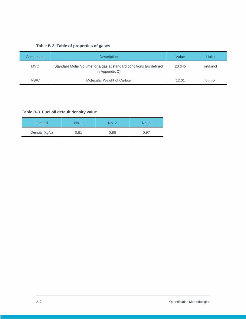
217 Quantifcation Methodologies
Table B-2. Table of properties of gases
Component Description Value Units
MVC Standard Molar Volume for a gas at standard conditions (as defined
in Appendix C)
23.645 m3/kmol
MWC Molecular Weight of Carbon 12.01 t/t-mol
Table B-3. Fuel oil default density value
Fuel Oil No. 1 No. 2 No. 6
Density (kg/L) 0.81 0.86 0.97

218 Quantifcation Methodologies
APPENDIX C: General Calculation Instructions C.1 Weighted average carbon content
Use Equation C.1-1 to calculate the weighted average carbon content of the fuel, if the measured
carbon content is used to calculate CO2 emissions. The units of measure for carbon content for
gaseous, liquid, and solid fuels are as follows:
Carbon Content Units of Measure:
Gaseous Fuels: kilograms of carbon per cubic metre of fuel (kg C/m3)
Liquid Fuels: tonnes of carbon per kilolitre of fuel (tonnes C/kl)
Solid Fuels: tonnes of carbon per tonne of fuel
To apply the carbon content in the equations outlined for various quantification methods, the
facility must ensure that the correct units are applied in the equation. Equation C.1-1a provides a
common conversion from mole fraction to mass fraction for gaseous fuels.
𝑪𝑪𝒑 = ∑ 𝑪𝑪𝒊×𝑭𝒖𝒆𝒍𝒊
𝑵𝒊=𝟏
∑ 𝑭𝒖𝒆𝒍𝒊𝑵𝒊=𝟏
Equation C.1-1
Where:
CCp = Weighted average carbon content of the fuel during the reporting
period, p.
CCi = Carbon content of the fuel for sampling period i.
Fueli = Quantity of fuel combusted during sampling period i:
Cubic metres (m3) for gaseous fuels.
Kilolitres (kl) for liquid fuels.
Tonnes for solid fuels
N = Number of measurement periods in the reporting period, in accordance
with Chapter 17.
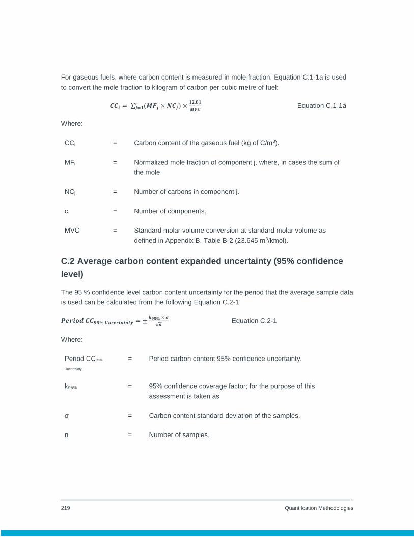
219 Quantifcation Methodologies
For gaseous fuels, where carbon content is measured in mole fraction, Equation C.1-1a is used
to convert the mole fraction to kilogram of carbon per cubic metre of fuel:
𝑪𝑪𝒊 = ∑ (𝑴𝑭𝒋 × 𝑵𝑪𝒋)𝒄𝒋=𝟏 ×
𝟏𝟐.𝟎𝟏
𝑴𝑽𝑪 Equation C.1-1a
Where:
CCi = Carbon content of the gaseous fuel (kg of C/m3).
MFi = Normalized mole fraction of component j, where, in cases the sum of
the mole
NCj = Number of carbons in component j.
c = Number of components.
MVC = Standard molar volume conversion at standard molar volume as
defined in Appendix B, Table B-2 (23.645 m3/kmol).
C.2 Average carbon content expanded uncertainty (95% confidence
level)
The 95 % confidence level carbon content uncertainty for the period that the average sample data
is used can be calculated from the following Equation C.2-1
𝑷𝒆𝒓𝒊𝒐𝒅 𝑪𝑪𝟗𝟓% 𝑼𝒏𝒄𝒆𝒓𝒕𝒂𝒊𝒏𝒕𝒚 = ±𝒌𝟗𝟓% × 𝝈
√𝒏 Equation C.2-1
Where:
Period CC95%
Uncertainty
= Period carbon content 95% confidence uncertainty.
k95% = 95% confidence coverage factor; for the purpose of this
assessment is taken as
σ = Carbon content standard deviation of the samples.
n = Number of samples.

220 Quantifcation Methodologies
This calculation instruction is to be used if the Director requests the calculation and reporting of
the carbon content uncertainty.
C.3 Fuel gas molecular weight estimation
If the molecular weight (MW) of the fuel gas is not measured, the molecular weight of the fuel gas
should be calculated by the summation of the mole fraction of each fuel gas component multiplied
by its respective molecular weight, as shown in the following equation.
𝑴𝑾 = ∑ 𝒙𝒊𝑴𝑾𝒊 Equation C.3-1
Where:
MW = Molecular weight of fuel gas (kg/kmol)
xi = Normalized mole fraction of component i, where, in cases the sum of
the mole
MW i = Molecular weight of component (kg/kmol), using Table B-1, Appendix B.
C.4 Standard temperature and pressure or standard conditions
In the document, standard conditions for pressure and temperature is 101.325 kPa (1 atm) and
15ºC (288.15K), respectively. If the gas volume is metered or recorded at different conditions, the
following equation should be used to convert gas volumes to standard gas volumes.
𝝊𝒔 = 𝟐. 𝟖𝟒𝟑𝟖 × 𝑷×𝝊
𝑻 Equation C.4-1
Where:
νs = Gas volume at standard conditions.
P = Pressure under which the gas volume is metered or recorded (kPa).
T = Temperature under which the gas volume is metered or recorded, in
Kelvin degrees.
ν = Gas volume at the metered or recorded conditions.

221 Quantifcation Methodologies
2.8438 = Constant for converting gas volumes to the standard condition (K/kPa).
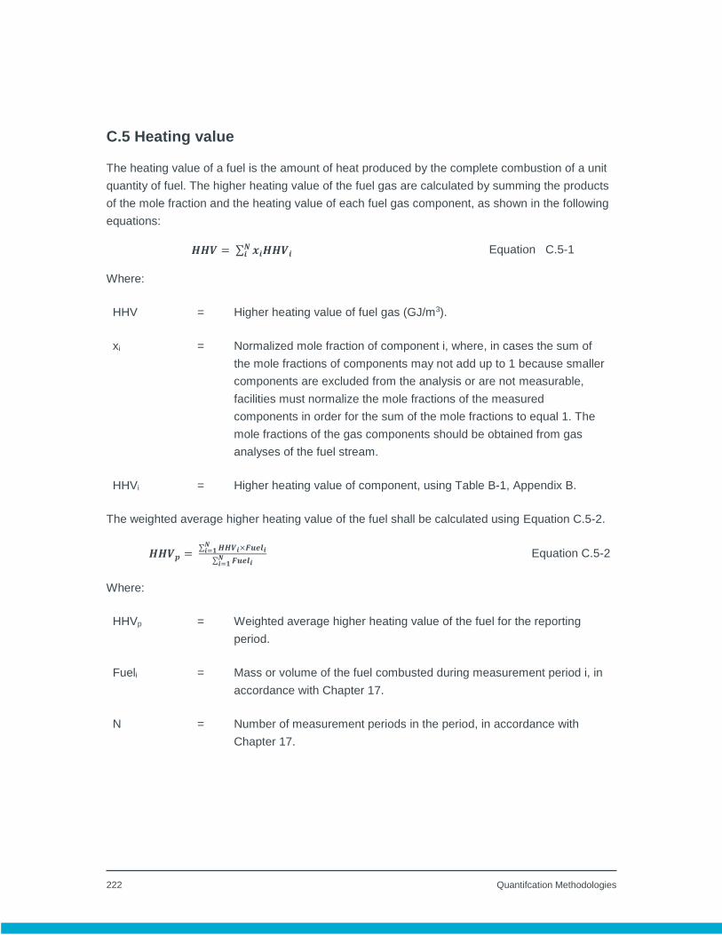
222 Quantifcation Methodologies
C.5 Heating value
The heating value of a fuel is the amount of heat produced by the complete combustion of a unit
quantity of fuel. The higher heating value of the fuel gas are calculated by summing the products
of the mole fraction and the heating value of each fuel gas component, as shown in the following
equations:
𝑯𝑯𝑽 = ∑ 𝒙𝒊𝑯𝑯𝑽𝒊𝑵𝒊 Equation C.5-1
Where:
HHV = Higher heating value of fuel gas (GJ/m3).
xi = Normalized mole fraction of component i, where, in cases the sum of
the mole fractions of components may not add up to 1 because smaller
components are excluded from the analysis or are not measurable,
facilities must normalize the mole fractions of the measured
components in order for the sum of the mole fractions to equal 1. The
mole fractions of the gas components should be obtained from gas
analyses of the fuel stream.
HHVi = Higher heating value of component, using Table B-1, Appendix B.
The weighted average higher heating value of the fuel shall be calculated using Equation C.5-2.
𝑯𝑯𝑽𝒑 = ∑ 𝑯𝑯𝑽𝒊×𝑭𝒖𝒆𝒍𝒊
𝑵𝒊=𝟏
∑ 𝑭𝒖𝒆𝒍𝒊𝑵𝒊=𝟏
Equation C.5-2
Where:
HHVp = Weighted average higher heating value of the fuel for the reporting
period.
Fueli = Mass or volume of the fuel combusted during measurement period i, in
accordance with Chapter 17.
N = Number of measurement periods in the period, in accordance with
Chapter 17.

223 Quantifcation Methodologies
HHVi = Higher heating value of the fuel, for measurement period i, in
accordance with Chapter 17.
C.6 Fuel consumption estimation
Facilities may estimate fuel consumption for combustion equipment based on equipment
specifications and operating hours using Equation C.6-1 or C.6-2.
𝒗𝒇𝒖𝒆𝒍,𝒋,𝒑 = ∑𝑷𝒓𝒂𝒕𝒆𝒅 𝒋
𝒏𝒋×
𝑳𝑭𝒋
𝑯𝑯𝑽𝒋× 𝑶𝑯𝒋 × 𝟎. 𝟎𝟎𝟑𝟔𝑵
𝒋=𝟏 Equation C.6-1
(e) 𝒗𝒇𝒖𝒆𝒍,𝒋,𝒑 = ∑ (𝑶𝑯𝒋 × 𝑯𝑷𝒋 × 𝑳𝑭𝒋 × 𝑩𝑺𝑭𝑪𝒋) × 𝟏𝟎−𝟑𝑵𝒋=𝟏 Equation C.6-2
Where:
vfuel,j,p = Estimated fuel consumption from combustion equipment for a specific fuel type
for the reporting period, p (m3).
j = Equipment type.
Prated j = Maximum rated power for equipment j (kW).
LFj = Load factor for each type of equipment j (dimensionless; ranges between 0 and
1).
OHj = Operating hours for equipment j (hours/reporting period).
nj = Thermal efficiency for equipment j.
HHVj = Higher heating value of the fuel combusted by equipment j (GJ/m3).
N = Number of equipment types using the same fuel.
HPj = Rated horsepower for equipment j (horsepower).
BSFCj = Brake-specific fuel consumption for equipment j in litres per horsepower-hour
(l/hp-h).
0.0036 = Conversion factor for kWh to GJ.
10-3 = Conversion factor for litres to cubic metres.
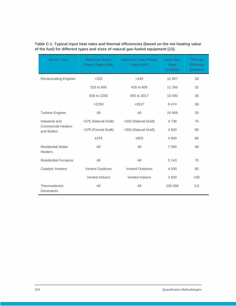
224 Quantifcation Methodologies
Table C-1. Typical input heat rates and thermal efficiencies (based on the net heating value
of the fuel) for different types and sizes of natural gas-fueled equipment [13].
Source Type Maximum Rated
Power Output (kW)
Maximum Rated Power
Output (HP)
Input Heat
Rate
(kJ/kWh)
Thermal
Efficiency
(percent)
Reciprocating Engines <325 <435 12 857 28
325 to 600 435 to 805 11 250 32
600 to 2250 805 to 3017 10 000 35
>2250 >3017 9 474 38
Turbine Engines All All 10 909 33
Industrial and
Commercial Heaters
and Boilers
<375 (Natural Draft) <503 (Natural Draft) 4 736 76
<375 (Forced Draft) <503 (Natural Draft) 4 500 80
≥375 ≥503 4 500 80
Residential Water
Heaters
All All 7 500 48
Residential Furnaces All All 5 143 70
Catalytic Heaters Vented Outdoors Vented Outdoors 4 500 80
Vented Indoors Vented Indoors 3 600 100
Thermoelectric
Generators
All All 100 000 3.6
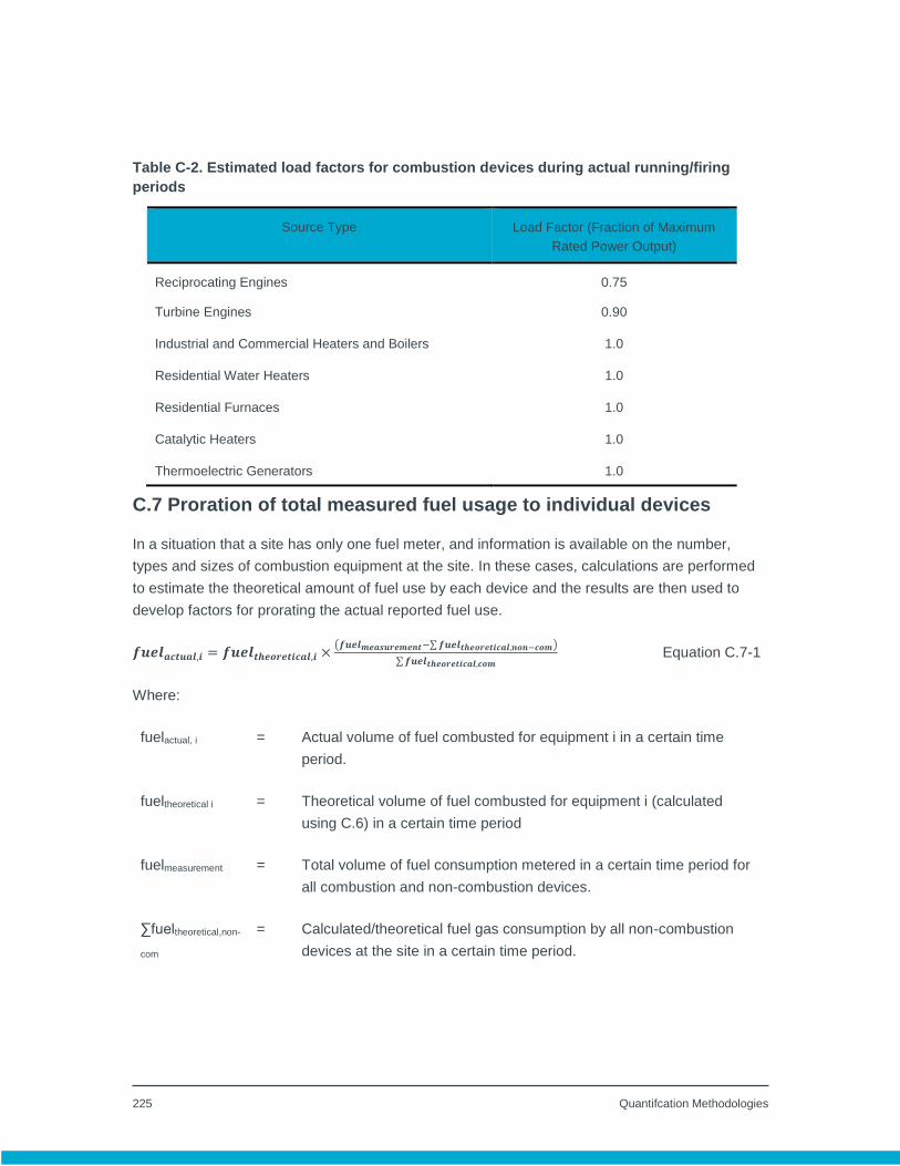
225 Quantifcation Methodologies
Table C-2. Estimated load factors for combustion devices during actual running/firing
periods
Source Type Load Factor (Fraction of Maximum
Rated Power Output)
Reciprocating Engines 0.75
Turbine Engines 0.90
Industrial and Commercial Heaters and Boilers 1.0
Residential Water Heaters 1.0
Residential Furnaces 1.0
Catalytic Heaters 1.0
Thermoelectric Generators 1.0
C.7 Proration of total measured fuel usage to individual devices
In a situation that a site has only one fuel meter, and information is available on the number,
types and sizes of combustion equipment at the site. In these cases, calculations are performed
to estimate the theoretical amount of fuel use by each device and the results are then used to
develop factors for prorating the actual reported fuel use.
𝒇𝒖𝒆𝒍𝒂𝒄𝒕𝒖𝒂𝒍,𝒊 = 𝒇𝒖𝒆𝒍𝒕𝒉𝒆𝒐𝒓𝒆𝒕𝒊𝒄𝒂𝒍,𝒊 ×(𝒇𝒖𝒆𝒍𝒎𝒆𝒂𝒔𝒖𝒓𝒆𝒎𝒆𝒏𝒕−∑ 𝒇𝒖𝒆𝒍𝒕𝒉𝒆𝒐𝒓𝒆𝒕𝒊𝒄𝒂𝒍,𝒏𝒐𝒏−𝒄𝒐𝒎)
∑ 𝒇𝒖𝒆𝒍𝒕𝒉𝒆𝒐𝒓𝒆𝒕𝒊𝒄𝒂𝒍,𝒄𝒐𝒎 Equation C.7-1
Where:
fuelactual, i = Actual volume of fuel combusted for equipment i in a certain time
period.
fueltheoretical i = Theoretical volume of fuel combusted for equipment i (calculated
using C.6) in a certain time period
fuelmeasurement = Total volume of fuel consumption metered in a certain time period for
all combustion and non-combustion devices.
∑fueltheoretical,non-
com
= Calculated/theoretical fuel gas consumption by all non-combustion
devices at the site in a certain time period.
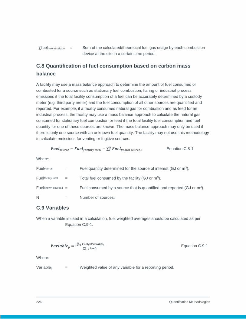
226 Quantifcation Methodologies
∑fueltheoretical,com = Sum of the calculated/theoretical fuel gas usage by each combustion
device at the site in a certain time period.
C.8 Quantification of fuel consumption based on carbon mass
balance
A facility may use a mass balance approach to determine the amount of fuel consumed or
combusted for a source such as stationary fuel combustion, flaring or industrial process
emissions if the total facility consumption of a fuel can be accurately determined by a custody
meter (e.g. third party meter) and the fuel consumption of all other sources are quantified and
reported. For example, if a facility consumes natural gas for combustion and as feed for an
industrial process, the facility may use a mass balance approach to calculate the natural gas
consumed for stationary fuel combustion or feed if the total facility fuel consumption and fuel
quantity for one of these sources are known. The mass balance approach may only be used if
there is only one source with an unknown fuel quantity. The facility may not use this methodology
to calculate emissions for venting or fugitive sources.
𝑭𝒖𝒆𝒍𝒔𝒐𝒖𝒓𝒄𝒆 = 𝑭𝒖𝒆𝒍𝒇𝒂𝒄𝒊𝒍𝒊𝒕𝒚 𝒕𝒐𝒕𝒂𝒍 − ∑ 𝑭𝒖𝒆𝒍𝒌𝒏𝒐𝒘𝒏 𝒔𝒐𝒖𝒓𝒄𝒆,𝒊𝑵𝒊 Equation C.8-1
Where:
Fuelsource = Fuel quantity determined for the source of interest (GJ or m3).
Fuelfacility total = Total fuel consumed by the facility (GJ or m3).
Fuelknown source,i = Fuel consumed by a source that is quantified and reported (GJ or m3).
N = Number of sources.
C.9 Variables
When a variable is used in a calculation, fuel weighted averages should be calculated as per
Equation C.9-1.
𝑽𝒂𝒓𝒊𝒂𝒃𝒍𝒆𝒑 =∑ 𝑭𝒖𝒆𝒍𝒊×𝑽𝒂𝒓𝒊𝒂𝒃𝒍𝒆𝒊
𝑵𝒊=𝟏
∑ 𝑭𝒖𝒆𝒍𝒊𝒏𝒊=𝟏
Equation C.9-1
Where:
Variablep = Weighted value of any variable for a reporting period.
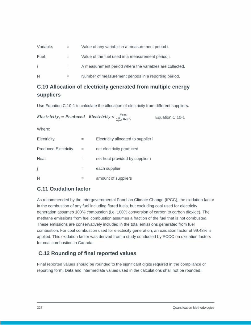
227 Quantifcation Methodologies
Variablei = Value of any variable in a measurement period i.
Fueli = Value of the fuel used in a measurement period i.
i = A measurement period where the variables are collected.
N = Number of measurement periods in a reporting period.
C.10 Allocation of electricity generated from multiple energy
suppliers
Use Equation C.10-1 to calculate the allocation of electricity from different suppliers.
𝑬𝒍𝒆𝒄𝒕𝒓𝒊𝒄𝒊𝒕𝒚𝒊 = 𝑷𝒓𝒐𝒅𝒖𝒄𝒆𝒅 𝑬𝒍𝒆𝒄𝒕𝒓𝒊𝒄𝒊𝒕𝒚 × 𝑯𝒆𝒂𝒕𝒊
∑ 𝑯𝒆𝒂𝒕𝒋𝑵𝒋=𝟏
Equation C.10-1
Where:
Electricityi = Electricity allocated to supplier i
Produced Electricity = net electricity produced
Heati = net heat provided by supplier i
j = each supplier
N = amount of suppliers
C.11 Oxidation factor
As recommended by the Intergovernmental Panel on Climate Change (IPCC), the oxidation factor
in the combustion of any fuel including flared fuels, but excluding coal used for electricity
generation assumes 100% combustion (i.e. 100% conversion of carbon to carbon dioxide). The
methane emissions from fuel combustion assumes a fraction of the fuel that is not combusted.
These emissions are conservatively included in the total emissions generated from fuel
combustion. For coal combustion used for electricity generation, an oxidation factor of 99.48% is
applied. This oxidation factor was derived from a study conducted by ECCC on oxidation factors
for coal combustion in Canada.
C.12 Rounding of final reported values
Final reported values should be rounded to the significant digits required in the compliance or
reporting form. Data and intermediate values used in the calculations shall not be rounded.
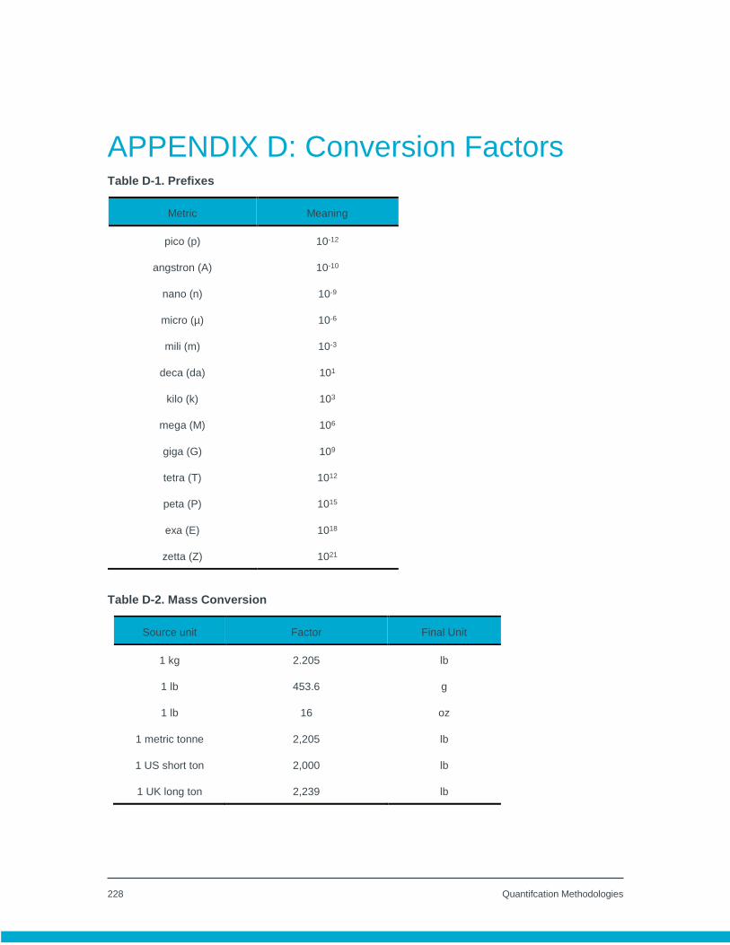
228 Quantifcation Methodologies
APPENDIX D: Conversion Factors Table D-1. Prefixes
Metric Meaning
pico (p) 10-12
angstron (A) 10-10
nano (n) 10-9
micro (µ) 10-6
mili (m) 10-3
deca (da) 101
kilo (k) 103
mega (M) 106
giga (G) 109
tetra (T) 1012
peta (P) 1015
exa (E) 1018
zetta (Z) 1021
Table D-2. Mass Conversion
Source unit Factor Final Unit
1 kg 2.205 lb
1 lb 453.6 g
1 lb 16 oz
1 metric tonne 2,205 lb
1 US short ton 2,000 lb
1 UK long ton 2,239 lb

229 Quantifcation Methodologies
Table D-3. Volume Conversion
Source unit Factor Final Unit
1 l 0.264 gal
1 gal 3.785 l
1 m3 35.3 ft3
1 ft3 28.32 l
1 ft3 7.482 gal
1 bbl 42 gal
1 bbl 158.9 l
1 bbl 5.6 ft3
Table D-4. Temperature Conversion
Source unit Factor
ºF 9 / 5 * ºC +32
ºC (ºF – 32) * 5 / 9
ºK ºC + 273.15
ºR ºF +459.67

230 Quantifcation Methodologies
Table D-5. Pressure Conversion
Source unit Factor Final Unit
1 MPa 0.1 bar
1 MPa 9.87 atm
1 MPa 145 psi
1 atm 1.0132 bar
1 atm 780 mmHg
1 atm 14.696 psi
Table D-6. Distance Conversion
Source unit Factor Final Unit
1 cm 0.3937 in
1 m 3.281 ft
1 m 1.094 yd
1 km 0.62137 mi
1 mi 1.609 km
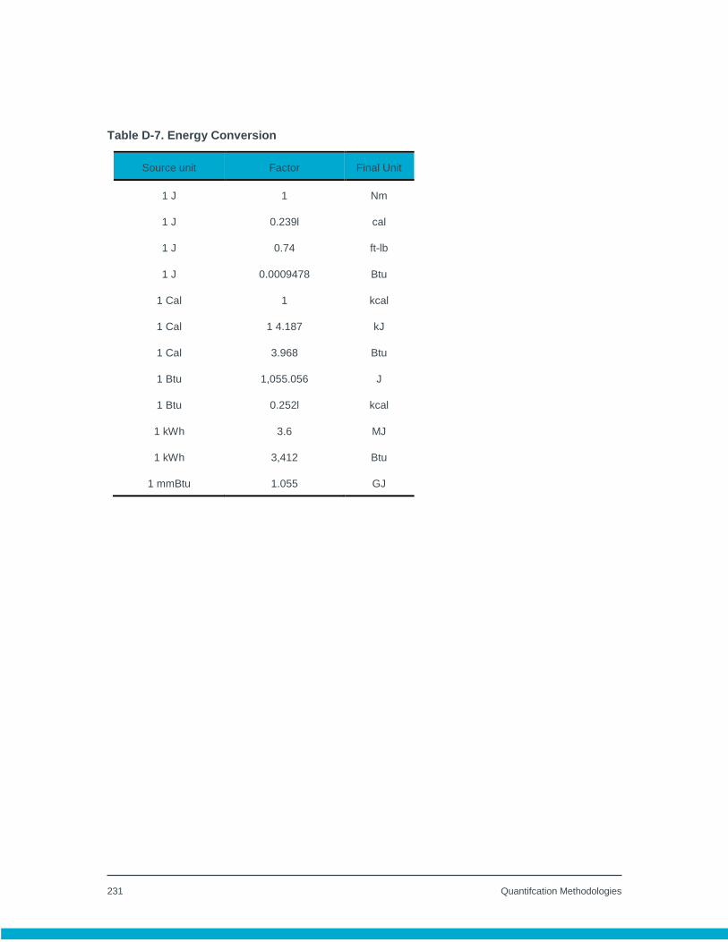
231 Quantifcation Methodologies
Table D-7. Energy Conversion
Source unit Factor Final Unit
1 J 1 Nm
1 J 0.239l cal
1 J 0.74 ft-lb
1 J 0.0009478 Btu
1 Cal 1 kcal
1 Cal 1 4.187 kJ
1 Cal 3.968 Btu
1 Btu 1,055.056 J
1 Btu 0.252l kcal
1 kWh 3.6 MJ
1 kWh 3,412 Btu
1 mmBtu 1.055 GJ

232 Quantifcation Methodologies
APPENDIX E: Alberta Gas Processing Index E.1 - Overview of Natural Gas Processing Modules
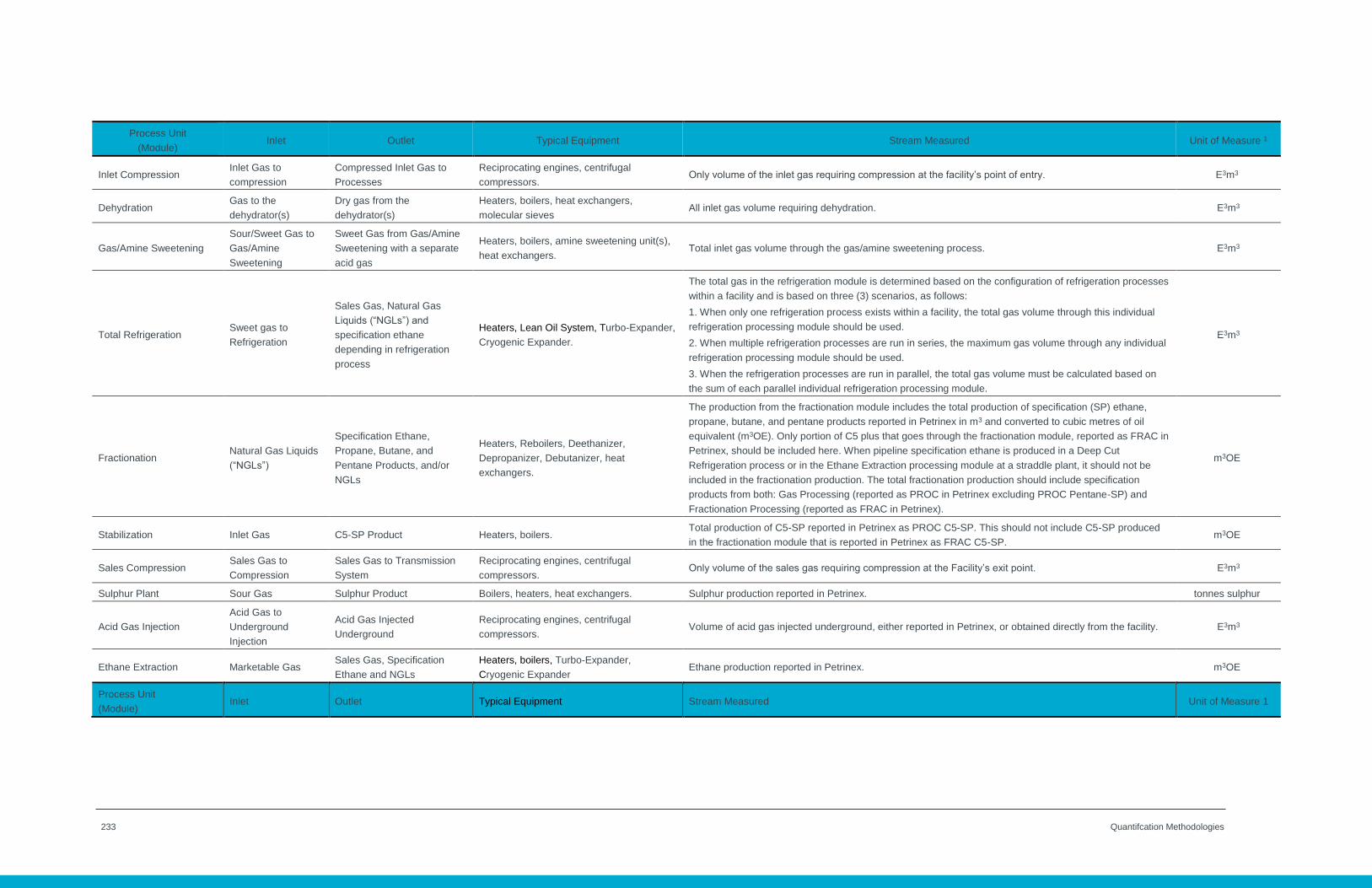
233 Quantifcation Methodologies
Process Unit
(Module) Inlet Outlet Typical Equipment Stream Measured Unit of Measure 1
Inlet Compression Inlet Gas to
compression
Compressed Inlet Gas to
Processes
Reciprocating engines, centrifugal
compressors. Only volume of the inlet gas requiring compression at the facility’s point of entry. E3m3
Dehydration Gas to the
dehydrator(s)
Dry gas from the
dehydrator(s)
Heaters, boilers, heat exchangers,
molecular sieves All inlet gas volume requiring dehydration. E3m3
Gas/Amine Sweetening
Sour/Sweet Gas to
Gas/Amine
Sweetening
Sweet Gas from Gas/Amine
Sweetening with a separate
acid gas
Heaters, boilers, amine sweetening unit(s),
heat exchangers. Total inlet gas volume through the gas/amine sweetening process. E3m3
Total Refrigeration Sweet gas to
Refrigeration
Sales Gas, Natural Gas
Liquids (“NGLs”) and
specification ethane
depending in refrigeration
process
Heaters, Lean Oil System, Turbo-Expander,
Cryogenic Expander.
The total gas in the refrigeration module is determined based on the configuration of refrigeration processes
within a facility and is based on three (3) scenarios, as follows:
1. When only one refrigeration process exists within a facility, the total gas volume through this individual
refrigeration processing module should be used.
2. When multiple refrigeration processes are run in series, the maximum gas volume through any individual
refrigeration processing module should be used.
3. When the refrigeration processes are run in parallel, the total gas volume must be calculated based on
the sum of each parallel individual refrigeration processing module.
E3m3
Fractionation Natural Gas Liquids
(“NGLs”)
Specification Ethane,
Propane, Butane, and
Pentane Products, and/or
NGLs
Heaters, Reboilers, Deethanizer,
Depropanizer, Debutanizer, heat
exchangers.
The production from the fractionation module includes the total production of specification (SP) ethane,
propane, butane, and pentane products reported in Petrinex in m3 and converted to cubic metres of oil
equivalent (m3OE). Only portion of C5 plus that goes through the fractionation module, reported as FRAC in
Petrinex, should be included here. When pipeline specification ethane is produced in a Deep Cut
Refrigeration process or in the Ethane Extraction processing module at a straddle plant, it should not be
included in the fractionation production. The total fractionation production should include specification
products from both: Gas Processing (reported as PROC in Petrinex excluding PROC Pentane-SP) and
Fractionation Processing (reported as FRAC in Petrinex).
m3OE
Stabilization Inlet Gas C5-SP Product Heaters, boilers. Total production of C5-SP reported in Petrinex as PROC C5-SP. This should not include C5-SP produced
in the fractionation module that is reported in Petrinex as FRAC C5-SP. m3OE
Sales Compression Sales Gas to
Compression
Sales Gas to Transmission
System
Reciprocating engines, centrifugal
compressors. Only volume of the sales gas requiring compression at the Facility’s exit point. E3m3
Sulphur Plant Sour Gas Sulphur Product Boilers, heaters, heat exchangers. Sulphur production reported in Petrinex. tonnes sulphur
Acid Gas Injection
Acid Gas to
Underground
Injection
Acid Gas Injected
Underground
Reciprocating engines, centrifugal
compressors. Volume of acid gas injected underground, either reported in Petrinex, or obtained directly from the facility. E3m3
Ethane Extraction Marketable Gas Sales Gas, Specification
Ethane and NGLs
Heaters, boilers, Turbo-Expander,
Cryogenic Expander Ethane production reported in Petrinex. m3OE
Process Unit
(Module) Inlet Outlet Typical Equipment Stream Measured Unit of Measure 1

234 Quantifcation Methodologies
Cavern Storage
Liquefied Gas
products, i.e.
Ethane, Propane,
Butane and asso-
ciated mixtures
Liquefied Gas products, i.e.
Ethane, Propane, Butane
and associated mixtures
stored in Cavern
Reciprocating engines, centrifugal
compressors. Total volume of the liquefied gas product(s) injected into the cavern(s). m3
CO2 Plant
Acid Gas from
Amine Sweetening
to the CO2 Plant
Gaseous or Liquid CO2
Product
Cryogenic technology equipment involving
the removal of CO2 from the gas stream,
including CO2 purification and/or
liquefaction.
Total CO2 gas volume from the amine sweetening through the CO2 removal and purification process. E3m3
Flaring, Venting,
Fugitives, Other
Various Natural Gas
Streams throughout
Process
Units/Modules
Various Natural Gas Streams
throughout Process
Units/Modules
Flare and Incinerator stacks, venting, facility
fugitive, residue gas for straddle plants,
diesel emergency generators, fire water
pumps and some other emission sources.
Total annual facility production reported in Petrinex. m3OE
All volumetric units should match standard conditions as defined in Petrinex. Standard conditions for calculating and reporting gas and liquid volumes are 101.325 kPa (absolute) and 15oC. Monthly gas volumes are reported in units of 103 m3 . The units for Cavern Storage (m3) will be
subject of a further review.
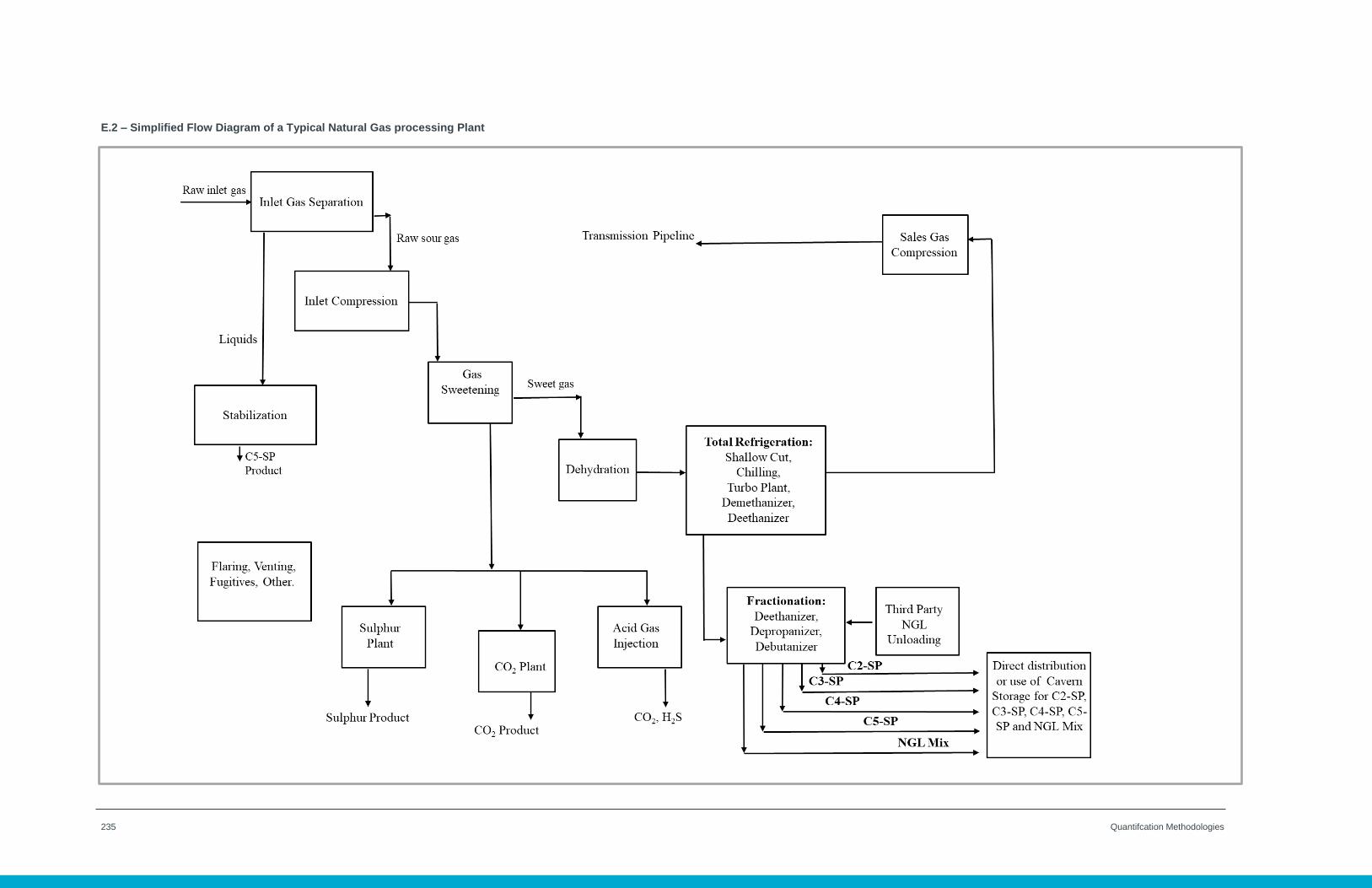
235 Quantifcation Methodologies
E.2 – Simplified Flow Diagram of a Typical Natural Gas processing Plant

236 Quantifcation Methodologies
E.3 – Simplified Flow Diagram of a Typical Natural Gas processing Plant (Dehydration within Refrigeration)

237 Quantifcation Methodologies
E.4 – Simplified Flow Diagram of a Typical Natural Gas Straddle Plant
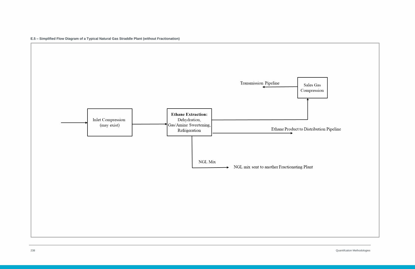
238 Quantifcation Methodologies
E.5 – Simplified Flow Diagram of a Typical Natural Gas Straddle Plant (without Fractionation)
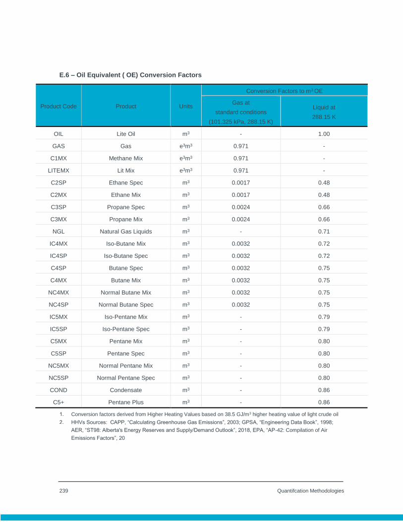
239 Quantifcation Methodologies
E.6 – Oil Equivalent ( OE) Conversion Factors
Product Code Product Units
Conversion Factors to m3 OE
Gas at
standard conditions
(101.325 kPa, 288.15 K)
Liquid at
288.15 K
OIL Lite Oil m3 - 1.00
GAS Gas e3m3 0.971 -
C1MX Methane Mix e3m3 0.971 -
LITEMX Lit Mix e3m3 0.971 -
C2SP Ethane Spec m3 0.0017 0.48
C2MX Ethane Mix m3 0.0017 0.48
C3SP Propane Spec m3 0.0024 0.66
C3MX Propane Mix m3 0.0024 0.66
NGL Natural Gas Liquids m3 - 0.71
IC4MX Iso-Butane Mix m3 0.0032 0.72
IC4SP Iso-Butane Spec m3 0.0032 0.72
C4SP Butane Spec m3 0.0032 0.75
C4MX Butane Mix m3 0.0032 0.75
NC4MX Normal Butane Mix m3 0.0032 0.75
NC4SP Normal Butane Spec m3 0.0032 0.75
IC5MX Iso-Pentane Mix m3 - 0.79
IC5SP Iso-Pentane Spec m3 - 0.79
C5MX Pentane Mix m3 - 0.80
C5SP Pentane Spec m3 - 0.80
NC5MX Normal Pentane Mix m3 - 0.80
NC5SP Normal Pentane Spec m3 - 0.80
COND Condensate m3 - 0.86
C5+ Pentane Plus m3 - 0.86
Conversion factors derived from Higher Heating Values based on 38.5 GJ/m3 higher heating value of light crude oil
HHVs Sources: CAPP, “Calculating Greenhouse Gas Emissions”, 2003; GPSA, “Engineering Data Book”, 1998;
AER, “ST98: Alberta's Energy Reserves and Supply/Demand Outlook”, 2018, EPA, “AP-42: Compilation of Air
Emissions Factors”, 20
Related Documents