SUMMARY OF EXPERIMENTAL UNCERTAINTY ASSESSMENT METHODOLOGY WITH EXAMPLE by Fred Stern, Marian Muste, Maria-Laura Beninati, and William E. Eichinger IIHR Technical Report No. 406 Iowa Institute of Hydraulic Research College of Engineering The University of Iowa Iowa City, Iowa 52242 July 1999

Welcome message from author
This document is posted to help you gain knowledge. Please leave a comment to let me know what you think about it! Share it to your friends and learn new things together.
Transcript
SUMMARY OF EXPERIMENTAL UNCERTAINTY
ASSESSMENT METHODOLOGY WITH EXAMPLE
by
Fred Stern, Marian Muste, Maria-Laura Beninati, and William E. Eichinger
IIHR Technical Report No. 406
Iowa Institute of Hydraulic Research College of Engineering The University of Iowa Iowa City, Iowa 52242
July 1999

i
TABLE OF CONTENTS
Abstract...............................................................................................................................iii
Acknowledgments ..............................................................................................................iii
1. Introduction ....................................................................................................................1
2. Test Design Philosophy..................................................................................................2
3. Accuracy, Errors, and Uncertainty .................................................................................4
4. Measurement Systems, Data-Reduction Equations, and Error Sources.........................6
5. Derivation of Uncertainty Propagation Equation ...........................................................8
6. Uncertainty Equations for Single and Multiple Tests ..................................................12
6.1 Bias Limits.......................................................................................................12
6.2 Precision Limits for Single Tests ....................................................................13
6.3 Precision Limits for Multiple Tests .....................……………………………14
7. Implementation.............................................................................................................15
8. Example for Measurement of Density and Kinematic Viscosity .................................16
8.1 Test Design ......................................................................................................17
8.2 Measurement Systems and Procedures ...........................................................18
8.3 Test Results......................................................................................................20
8.4 Uncertainty Assessment ..................................................................................20
8.4.1 Multiple Tests ...................................................................................21
8.4.2 Single Test ........................................................................................25
8.5 Discussion of Results ......................................................................................27
8.6 Comparison with Benchmark Data .................................................................28
9. Conclusions and Recommendations.............................................................................32
References .........................................................................................................................34
Appendix A. Individual Variable Precision Limit ...........................................................35

ii
LIST OF FIGURES
Figure Page
1. Integration of uncertainty assessment in test process (AIAA, 1995) ............................3
2. Errors in the measurement of a variable X (Coleman and Steele, 1995).......................5
3. Propagation of errors into experimental results (AIAA, 1995) .....................................7
4. Sources of errors (adapted AIAA, 1995).......................................................................7
5. Schematic of error propagation from a measured variable into the result.....................8
6. Propagation of bias and precision errors into a two variable result
(Coleman and Steele, 1995).........................................................................................10
7. Experimental arrangement...........................................................................................17
8. Block diagram of experiment ......................................................................................19
9. Density of 99.7% aqueous glycerin solution test results and comparison with
benchmark data..................................................................................................................31
10. Kinematic viscosity of 99.7% aqueous glycerin solution test results and
comparison with benchmark data ................................................................................32
LIST OF TABLES
Table Page
1. Gravity and sphere density constants ..........................................................................20
2. Typical test results .......................................................................................................20
3. Bias limits for individual variables D and t .................................................................22
4. Uncertainty estimates for density using multiple test method.....................................23
5. Uncertainty estimates for kinematic viscosity (teflon spheres) using
multiple test method ....................................................................................................25
6. Uncertainty estimates for density using single test method ........................................27
7. Uncertainty estimates for kinematic viscosity (teflon spheres) using
single test method ........................................................................................................27
8. Total uncertainty estimates for density and kinematic viscosity of glycerin
(values in parenthesis include consideration of correlated bias errors).......................28

iii
Abstract
A summary is provided of the AIAA Standard (1995) for experimental
uncertainty assessment methodology that is accessible and suitable for student and
faculty use both in classroom and research laboratories. To aid in application of the
methodology for academic purposes, also provided are a test design philosophy; an
example for measurement of density and kinematic viscosity; and recommendations for
application/integration of uncertainty assessment methodology into the test process and
for documentation of results. Additionally, recommendations for laboratory
administrators are included.
Acknowledgements
To insure accuracy, the summary is taken from the AIAA Standard and Coleman
and Steele (1995). The work has greatly benefited from collaboration with the 22nd
International Towing Tank Conference (ITTC) Resistance Committee through F. Stern.
M. Muste and M. Beninati were partially supported by The University of Iowa, College
of Engineering funds for fluids laboratory development and teaching assistants,
respectively. Ms. A. Williams helped in data acquisition and reduction during the
summer of 1998 as an undergraduate teaching assistant supported by The University of
Iowa, College of Engineering funds for fluids laboratory development.

1
1. Introduction
Experiments are an essential and integral tool for engineering and science in
general. By definition, experimentation is a procedure for testing (and determination) of
a truth, principle, or effect. However, the true values of measured variables are seldom
(if ever) known and experiments inherently have errors, e.g., due to instrumentation, data
acquisition and reduction limitations, and facility and environmental effects. For these
reasons, determination of truth requires estimates for experimental errors, which are
referred to as uncertainties. Experimental uncertainty estimates are imperative for risk
assessments in design both when using data directly or in calibrating and/or validating
simulation methods.
Rigorous methodologies for experimental uncertainty assessment have been
developed over the past 50 years. Standards and guidelines have been put forth by
professional societies (ANSI/ASME, 1985) and international organizations (ISO, 1993).
Recent efforts are focused on uniform application and reporting of experimental
uncertainty assessment.
In particular the American Institute of Aeronautics and Astronautics (AIAA) in
conjunction with Working Group 15 of the Advisory Group for Aerospace Research and
Development (AGARD) Fluid Dynamics Panel has put forth a standard for assessment of
wind tunnel data uncertainty (AIAA, 1995). This standard was developed with the
objectives of providing a rational and practical framework for quantifying and reporting
uncertainty in wind tunnel test data. The quantitative assessment method was to be
compatible with existing methodologies within the technical community. Uncertainties
that are difficult to quantify were to be identified and guidelines given on how to report
these uncertainties. Additional considerations included: integration of uncertainty
analyses into all phases of testing; simplified analysis while focusing on primary error
sources; incorporation of recent technical contributions such as correlated bias errors and
methods for small sample sizes; and complete professional analysis and documentation of
uncertainty for each test. The uncertainty assessment methodology has application to a
wide variety of engineering and scientific measurements and is based on Coleman &
Steele (1995, 1999), which is an update to the earlier standards.

2
The purpose of this report is to provide a summary of the AIAA Standard (1995)
for experimental uncertainty assessment methodology that is accessible and suitable for
student and faculty use both in the classroom and in research laboratories. To aid in the
application of the methodology for academic purposes, also provided are a test design
philosophy; an example for measurement of density and kinematic viscosity; and
recommendations for application/integration of uncertainty assessment methodology into
the test process and for documentation of results. Additionally, recommendations for
laboratory administrators are included.
.
2. Test Design Philosophy
Experiments have a wide range of purposes. Of particular interest are fluids
engineering experiments conducted for science and technological advancement; research
and development; design, test, and evaluation; and product liability and acceptance. Tests
include small-, model-, and full-scale with facilities ranging from table-top laboratory
experiments, to large-scale towing tanks and wind tunnels, to in situ experiments
including environmental effects. Examples of fluids engineering tests include: theoretical
model formulation; benchmark data for standardized testing and evaluation of facility
biases; simulation validation; instrumentation calibration; design optimization and
analysis; and product liability and acceptance.
Decisions on conducting experiments should be governed by the ability of the
expected test outcome to achieve the test objectives within the allowable uncertainties.
Thus, data quality assessment should be a key part of the entire experimental testing: test
description, determination of error sources, estimation of uncertainty, and documentation
of the results. A schematic of the experimental process, shown in Figure 1, illustrates
integration of uncertainty considerations into all phases of a testing process, including the
decision whether to test or not, the design of the experiments, and the conduct of the test.
Along with this philosophy of testing, rigorous application/integration of uncertainty
assessment methodology into the test process and documentation of results should be the
foundation of all experiments.

3
Figure 1. Integration of uncertainty assessment in test process (AIAA, 1995)
D E FINE P U R P O S E O F T E S T A NDR E SU LT S U NC E RTA IN TY R EQ U IR E M E NT S
U N CE RTA IN T YA C CE P TA BL E ?IM P R O VE M E N T
P O SS IB L E ?
D E TE R M IN E E RR O R S O U R C E SA FF E C TIN G RE S U LTS
Y E SN O
N O
Y E S Y E S
Y E S
N O
S E LE C T U N CE R TA IN T Y M E T HO D
E S TIM AT E E F FE C T O FT H E ER R O R S O N RE S U LTS
- M O D EL C O NF IG U R AT IO N S (S )- T E S T T E CH N IQ U E (S )- M E AS U R E M E N T S R EQ U IR E D- S P EC IF IC IN ST R U M EN TAT IO N- C O R R E C TIO N S TO B E A PP L IE D
- D E SIRE D PA R A M ET E R S (C , C ,....)D R
D E SIG N T HE T ES T
- R E FE R E NC E C O N D IT IO N- P R EC IS IO N L IM IT- B IA S L IM IT- TO TA L U N C E RTAIN TY
D O C U M E N T R E SU LT S
N O T E S T
C O N T IN U E T E S T
IM P L EM E N T TE S T
S O LVE P R O B LE M
R E SU LT SA C CE P TA BL E ?
M E A SU R E-M E N T
S YS TE MP RO BLE M ?
N O
P U RP O S EA C HIEV E D ?
Y E S
N O
S TAR T T E ST
E S TIM AT EA C TU A L D ATAU N CE RTA IN T Y

4
3. Accuracy, Errors, and Uncertainty
We consider here measurements made from calibrated instruments for which all
known systematic errors have been removed. Even the most carefully calibrated
instruments will have errors associated with the measurements, errors which we assume
will be equally likely to be positive and negative. The accuracy of a measurement
indicates the closeness of agreement between an experimentally determined value of a
quantity and its true value. Error is the difference between the experimentally determined
value and the true value. Accuracy increases as error approaches zero. In practice, the
true values of measured quantities are rarely known. Thus, one must estimate error and
that estimate is called an uncertainty, U. Usually, the estimate of an uncertainty, UX, in a
given measurement of a physical quantity, X, is made at a 95-percent confidence level.
This means that the true value of the quantity is expected to be within the ± U interval
about the mean 95 times out of 100.
As shown in Figure 2a, the total error, δ, is composed of two components: bias
error, β, and precision error, ε. An error is classified as precision error if it contributes to
the scatter of the data; otherwise, it is bias error. The effects of such errors on multiple
readings of a variable, X, are illustrated in Figure 2b.
If we make N measurements of some variable, the bias error gives the difference
between the mean (average) value of the readings, µ, and the true value of that variable.
For a single instrument measuring some variable, the bias errors, β, are fixed, systematic,
or constant errors (e.g., scale resolution). Being of fixed value, bias errors cannot be
determined statistically. The uncertainty estimate for β is called the bias limit, B. A
useful approach to estimating the magnitude of a bias error is to assume that the bias error
for a given case is a single realization drawn from some statistical parent distribution of
possible bias errors. The interval defined by ±B includes 95% of the possible bias errors
that could be realized from the parent distribution. For example, a thermistor for which
the manufacturer specifies that 95% of the samples of a given model are within ± 1.0 C°
of a reference resistance-temperature calibration curve supplied with the thermistor.
The precision errors, ε, are random errors and will have different values for each
measurement. When repeated measurements are made for fixed test conditions, precision
errors are observed as the scatter of the data. Precision errors are due to limitations on

5
repeatability of the measurement system and to facility and environmental effects.
Precision errors are estimated using statistical analysis, i.e., are assumed proportional to
the standard deviation of a sample of N measurements of a variable, X. The uncertainty
estimate of ε is called the precision limit, P.
Figure 2. Errors in the measurement of a variable X (Coleman and Steele, 1995)
δβε
= to ta l e rro r = b ias e rro r = p recis ion error
β
µM A G N ITU D E O F ;
FR
EQ
UE
NC
Y O
F O
CC
UR
RE
NC
E
�
�
�
WUXH
�WUXH
εN
ε ε
εN��
δN
δN��
N����
N
(a ) tw o read in g s
(b ) in f in ite nu m b e r o f read in g s
β

6
4. Measurement Systems, Data-Reduction Equations, and Error Sources
Measurement systems consist of the instrumentation, the procedures for data
acquisition and reduction, and the operational environment, e.g., laboratory, large-scale
specialized facility, and in situ. Measurements are made of individual variables, Xi, to
obtain a result, r, which is calculated by combining the data for various individual
variables through data reduction equations
)X ..., ,X ,X ,X ( r = r J321 (1)
For example, to obtain the velocity of some object, one might measure the time required
(X1) for the object to travel some distance (X2) in the data reduction equation V = X2 / X1.
Each of the measurement systems used to measure the value of an individual
variable, Xi, is influenced by various elemental error sources. The effects of these
elemental errors are manifested as bias errors (estimated by Bi) and precision errors
(estimated by Pi) in the measured values of the variable, Xi. These errors in the measured
values then propagate through the data reduction equation, thereby generating the bias,
Br, and precision, Pr, errors in the experimental result, r. Figure 3 provides a block
diagram showing elemental error sources, individual measurement systems, measurement
of individual variables, data reduction equations, and experimental results. Typical error
sources for measurement systems are shown in Figure 4.
Estimates of errors are meaningful only when considered in the context of the
process leading to the value of the quantity under consideration. In order to identify and
quantify error sources, two factors must be considered: (1) the steps used in the processes
to obtain the measurement of the quantity, and (2) the environment in which the steps
were accomplished. Each factor influences the outcome. The methodology for estimating
the uncertainties in measurements and in the experimental results calculated from them
must be structured to combine statistical and engineering concepts. This must be done in
a manner that can be systematically applied to each step in the data uncertainty
assessment determination. In the methodology discussed below, the 95% confidence
large-sample uncertainty assessment approach is used as recommended by the AIAA
(1995) for the vast majority of engineering tests.

7
Figure 3. Propagation of errors into experimental results (AIAA, 1995)
Figure 4. Sources of errors (adapted AIAA, 1995)
M O D EL FID E LIT Y AN DTE ST SET U P:- As bu ilt geom etry- H yd rodynam ic de fo rm a tion- S urface fin ish- M ode l p ositioning
TE ST EN VIR O N M EN T:- C alibration versu s test- Spatia l/tem pora l varia tions o f the f low- Se nso r ins ta lla tio n/lo cation- Wa ll in te rfe re nce- F luid an d fac ility conditions
D ATA AC Q U IS ITIO N AN DR ED U C TIO N :- S am pling, filte rin g, an d sta tis tics- C u rve fits- C a libra tions
S IM U LATIO N TE C H N IQ U ES :- Ins tru m en ta tion in te rfe rence- S ca le e ffec ts
C O N TR IBU T IO N STO EST IM ATEDU N C ER TAIN ITY
r = r (X , X ,......, X ) 1 2 J
1 2 J
M E AS UR E M E NTO F IND IV ID UA LVA R IAB LE S
IND IVID UA LM E AS UR E M E NTS Y STE MS
E LEM ENTA LE RR O R S O UR C ES
DATA RE DU CTIO NE Q UATIO N
E X PER IM EN TA LRE S ULT
XB , P
1
1 1
XB , P
2
2 2
XB , P
J
J J
rB , P
r r

8
5. Derivation of Uncertainty Propagation Equation
Bias and precision errors in the measurement of individual variables, Xi,
propagate through the data reduction equation (1) resulting in bias and precision errors in
the experimental result, r (Figure 3). One can see how a small error in one of the
measured variables propagates into the result by examining Figure 5. A small error, iXδ ,
in the measured value leads to a small error, δr, in the result that can be approximated
using a Taylor series expansion of r(Xi) about rtrue(Xi). The error in the result is given by
the product of the error in the measured variable and the derivative of the result with
respect to that variable idX
dr (i.e., slope of the data reduction equation). This
derivative is referred to as a sensitivity coefficient. The larger the derivative/slope, the
more sensitive the value of the result is to a small error in a measured variable.
Figure 5. Schematic of error propagation from a measured variable into the result
In the following, an overview of the derivation of an equation describing the error
propagation is given with particular attention to the assumptions and approximations
made to obtain the final uncertainty equation applicable for both single tests and multiple
δr
δX
r(X )i
trueX iX i
r
rtrue
r(X )i
X i
drdX i
i

9
tests (Section 6). A detailed derivation can be found in Coleman and Steele (1995).
Rather than presenting the derivation for a data reduction equation of many
variables, the simpler case in which equation (1) is a function of only two variables is
presented, hence
),( yxrr = (2)
The situation is shown in Figure 6 for the kth set of measurements (xk, yk) that is used to
determine rk. Here, kxβ and
kxε are the bias and precision errors, respectively, in the kth
measurement of x, with a similar convention for the errors in y and r. Assume that the
test instrumentation and/or apparatus is changed for each measurement so that different
values of kxβ and
kxε will occur for each measurement. Therefore, the bias and precision
errors will be random variables relating the measured and true values
kk xxtruek xx εβ ++= (3)
kk yytruek yy εβ ++= (4)
The error in rk (the difference between rtrue and rk) in equation (2) can be
approximated by a Taylor series expansion as
( ) ( ) 2Ryyy
rxx
x
rrr truektruektruek +−
∂∂+−
∂∂=− (5)
Neglecting higher order terms (term R2, etc.), substituting for (xk - xtrue) and (yk - ytrue) from
equations (3) and (4), and defining the sensitivity coefficients xrx ∂∂=θ and
yry ∂∂=θ , the total error δ in the kth determination of the result r is defined from
equation (5) as
( ) ( )kkkkk yyyxxxtruekr rr εβθεβθδ +++=−= (6)
Equation (6) shows that krδ is the product of the total errors in the measured variables
(x,y) with their respective sensitivity coefficients.

10
Figure 6. Propagation of bias and precision errors into a two variable result
(Coleman and Steele, 1995)
We are interested in obtaining a measure of the distribution of krδ for (some large
number) N determinations of the result r. The variance of this “parent” distribution is
defined by
( )
= ∑
=∞→
N
kr
N kr N 1
22 1lim δσδ (7)
Substituting equation (6) into equation (7), taking the limit as N approaches infinity,
using definitions of variances similar to that in equation (7) for the β’s, ε’s, and their
correlation, and assuming that there are no bias error/precision error correlations, results
in the equation for rδσ
yxxxyxyxr yxyxyxyx εεεεββββδ σθθσθσθσθθσθσθσ 22 222222222 +++++= (8)
Since in reality the various σ’s are not known exactly, estimates for them must be
made. Defining 2cu as an estimate for the variance of the total error distribution, 2
rδσ ,
xyyx bbb ,, 22 as estimates for the variances and covariance of the bias error distributions,
µ[ N
N
N N N
NWUXH WUXH
WUXH
N
N
N
N
N
N
β
β
ε
ε
U U [ � \ � �
[
U
[
U
U
[
[
U
\µ\
βε\
\
\

11
and, xyyx SSS ,, 22 , as estimates for the variances and covariances of the precision error
distributions, results in the equation for uc
xyyxyyxxxyyxyyxxc SSSbbbu θθθθθθθθ 22 222222222 +++++= (9)
bxy and Sxy are estimates of the correlated bias and precision errors, respectively, in x and
y.
No assumptions have yet been made on types of error distributions. To obtain an
uncertainty Ur at a specified confidence level (e.g., 95%), uc must be multiplied by a
coverage factor K
cr KuU = (10)
Choosing K requires assumptions on types of error distributions. We will assume that the
error distribution of the result, r, is normal so that we may replace the value of K for C%
coverage (corresponding to the C% confidence level) with the t value from the Student t
distribution. For sufficiently large number of measurements, N ≥10, t = 2 for 95%
confidence. With these final assumptions and generalizing equation (9) for the case in
which the experimental result r is obtained from equation (1) provides the desired result
∑ ∑ ∑∑ ∑ ∑=
−
= +==
−
= +=
+++J
i
J
i
J
ikikkiii
J
i
J
i
J
ikikkiiir PP BB = U
1
1
1 1
22
1
1
1 1
222 22 θθθθθθ (11)
where Bi=tbi, Bik=t2bik, Pi=tSi, Pik=t2Sik and t = 2 for N ≥10. With reference to Figure 3,
Bi and Pi are the bias limits in Xi; and Bik and Pik are the correlated bias and precision
limits in Xi and Xk. Si is the standard deviation for a sample of N readings of the variable
Xi. The sensitivity coefficients are defined as
i
i X
r
∂∂=θ (12)
Equation (11) is the desired propagation equation, which was setout to be derived. The
equation is used for both single tests and multiple tests as presented next in Section 6.

12
6. Uncertainty Equations for Single and Multiple Tests
A given set of measurements may be made in several different ways. Ideally,
one will be able to repeat the measurements several times. In multiple tests, the result r =
(X1, X2,…, XJ ) is determined from many sets of measurements (X1, X2,…,XJ) at a fixed
test condition with the same measurement systems. However, in some instances (e.g.,
complex or expensive experiments), it may not be possible to perform a test more than
once. For this situation the result r = (X1, X2,…, XJ ) is determined from one set of
measurements (X1, X2,…,XJ) at a fixed test condition. According to the present
methodology, a test is considered a single test if the entire test is performed only once,
even if the measurements of one or more of the variables are made from many samples.
For example, when measuring the dynamic pressure in a pipe, one may make many
samples over a period of time long enough to average out the effects of turbulence. The
average of these measurements is taken to be the measurement of that particular variable
so that a single value is available.
The total uncertainty in the result, r, for both single and multiple tests is the root-
sum-square (RSS) of the bias and precision limits
P + B = U 2r
2rr
2 (13)
The bias limits of the results [Br in equation (13)] for single and multiple tests are
determined in the same manner. The precision limits are determined differently
depending upon how the data was collected, i.e., single or multiple test.
6.1. Bias Limits
For both single and multiple tests, the bias limit of the result [Br in equation (13)] is
given by
∑ ∑ ∑=
−
= +=
+=J
i
J
i
J
ikikkiiir BBB
1
1
1 1
222 2 θθθ (14)
where iθ are the sensitivity coefficients defined as before

13
i
i X
r
∂∂=θ (15)
Bi are the bias limits in Xi and Bik are the correlated bias limits in Xi and Xk
( ) ( )∑=
=L
kiik BBB1α
αα (16)
L is the number of correlated bias error sources that are common for measurement of
variables Xi and Xk.
The bias limit Bi for each variable is an estimate of elemental bias errors from
different categories: calibration errors; data acquisition errors; data reduction errors; and
conceptual bias. Within each category, there may be several elemental sources of bias.
For instance, if for the ith variable Xi there are J elemental bias errors identified as
significant and whose bias limits are estimated as (Bi)1, (Bi)2, . . . , (Bi)J then the bias
limit for the measurement of Xi is calculated as the root-sum-square (RSS) combination
of the elemental limits
)B( = B 2ki
J
1=ki ∑2 (17)
The bias limits for each element (Bi)k must be estimated for each variable Xi using the
best information one has available at the time. In the design phase of an experimental
program, manufacturer's specifications, analytical estimates, and previous experience will
typically provide the basis for most of the estimates. As the experimental program
progresses, equipment is assembled, and calibrations are conducted, these estimates can
be updated using the additional information gained about the accuracy of the calibration
standards, errors associated with calibration process and curvefit procedures, and perhaps
analytical estimates of installation errors (e.g., wall interference effects).
6.2 Precision Limits for Single Tests
For single tests in which one or more of the measurements were made from many
samples over some time interval at a fixed test condition, and assuming no correlated
precision limits for the precision errors, the precision limit of the result [Pr in equation
14
(13)] can be estimated by
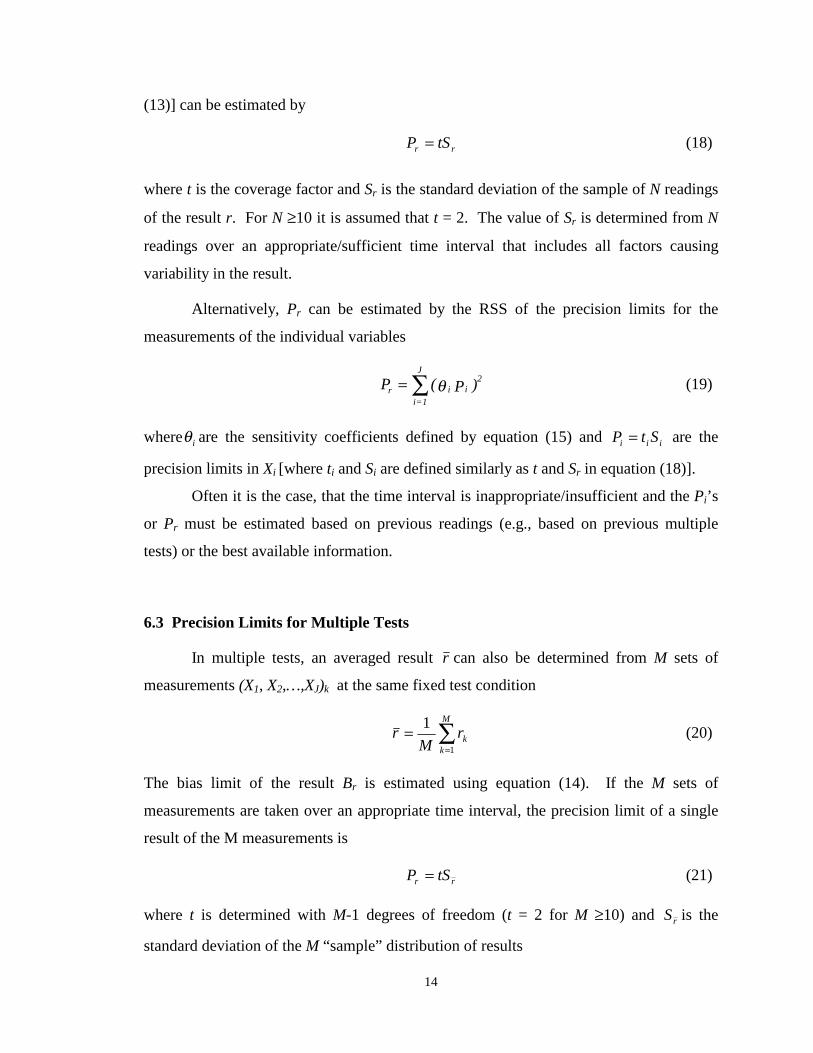
rr tSP = (18)
where t is the coverage factor and Sr is the standard deviation of the sample of N readings
of the result r. For N ≥10 it is assumed that t = 2. The value of Sr is determined from N
readings over an appropriate/sufficient time interval that includes all factors causing
variability in the result.
Alternatively, Pr can be estimated by the RSS of the precision limits for the
measurements of the individual variables
)P ( P 2ii
J
1=ir θ∑= (19)
where iθ are the sensitivity coefficients defined by equation (15) and iii StP = are the
precision limits in Xi [where ti and Si are defined similarly as t and Sr in equation (18)].
Often it is the case, that the time interval is inappropriate/insufficient and the Pi’s
or Pr must be estimated based on previous readings (e.g., based on previous multiple
tests) or the best available information.
6.3 Precision Limits for Multiple Tests
In multiple tests, an averaged result r can also be determined from M sets of
measurements (X1, X2,…,XJ)k at the same fixed test condition
∑=
=M
kkrM
r1
1 (20)
The bias limit of the result Br is estimated using equation (14). If the M sets of
measurements are taken over an appropriate time interval, the precision limit of a single
result of the M measurements is
rr tSP = (21)
where t is determined with M-1 degrees of freedom (t = 2 for M ≥10) and rS is the
standard deviation of the M “sample” distribution of results

15
( ) 2/1
1
2
1
−
−= ∑
=
M
k
kr M
rrS (22)
The precision limit for the average result is given by
M
tSP r
r = (23)
The total uncertainty for the average result is (using the large sample assumption)
( )22222 2 MSBPBU rrrrr +=+= (24)
Alternatively, r
P can be estimated as the RSS of the precision limits of the
individual variables
)P ( P 2ii
J
=1ir θ∑= (25)
where the precision limit of one of the measured variables is
M
tSP i
i= (26)
and t is taken to be 2 when the number of samples is greater than 10 and Si is the standard
deviation of the M sample results
( ) 2/1
1
2
1
−−
= ∑=
M
k
ik
i M
XXS (27)
7. Implementation
The uncertainty assessment methodology is summarized in Figure 1. For each
experimental result, the data reduction equation (1) is determined first. Then a block
diagram of the test (Figure 3) is constructed to help organize the individual measurement
systems and the propagation of elemental error sources into the final result. Data-stream
diagrams are constructed next, showing data flow from sensor-to-result and are helpful
for identification and organization of the elemental bias and precision limits at the

16
individual-variable level.
Bias limits contributing either to a single variable or the final result are identified
(calibration, data acquisition, data reduction, or conceptual bias) and combined. Once the
sources of uncertainty have been identified, their relative significance should be
established based on order of magnitude estimates. A “rule of thumb” is that those
uncertainty sources that are smaller that 1/4 or 1/5 of the largest sources are usually
considered negligible.
For the vast majority of experiments, precision limits are estimated as described
above with repeated end-to-end data-acquisition and reduction cycles (i.e., for the final
result level as opposed to the individual variable level). Note that the precision limit
computed is only applicable for those random error sources that were “active” during the
repeated measurements. Ideally M ≥ 10, however, often this is not the case and for M <
10, a coverage factor t = 2 is still permissible if the bias and precision limits have similar
magnitude. If one encounters unacceptably large P’s, the elemental sources'
contributions must be examined to see which need to be (or can be) improved.
The precision limit, bias limit, and total uncertainty for the experimental result r
are then found. For each experimental result, the bias limit, precision limit, and total
uncertainty should be reported.
8. Example for Measurement of Density and Kinematic Viscosity
Professor R. Ettema and Dr. M. Muste developed the present experiment at IIHR
during the summer of 1997 for use in the fluids lab. Subsequently, as presented herein,
the experiment was revised to include uncertainty assessment. Granger (1988) presents a
similar experiment, but without uncertainty assessment.
The experiment determines density and kinematic viscosity of a fluid by equating
forces on a sphere falling at terminal velocity and low Reynolds number (Roberson and
Crowe, 1997, pp. 438-443). More commonly, density is determined from specific weight
measurements using hydrometers (Roberson and Crowe, 1997, pg. 57) and viscosity is
determined using capillary viscometers.
The purpose of the experiment is to provide a relatively simple, yet
comprehensive, tabletop measurement system for demonstrating fluid mechanics

17
concepts, experimental procedures, and uncertainty assessment. The measurements are
compared with benchmark data based both on reference data provided by the fluid
(99.7% aqueous glycerin solution) manufacturer and measurements using a
commercially available hydrometer and capillary viscometer.
8.1. Test Design
A sphere of diameter D falls at terminal velocity V through a long transparent
cylinder filled with fluid of density ρ, viscosity µ, and kinematic viscosity ν (= µ/ρ), as
shown in Figure 7. The acceleration is zero, hence, the forces acting on the sphere must
sum to zero. These forces of gravity Fg, buoyancy Fb, and drag Fd, sum as:
dbga FFFW =−= (28)
Figure 7. Experimental arrangement
The apparent weight is given by
)1( −∇= SWa γ (29)
where γ = ρg is the specific weight of the fluid, ∇ = πD3/6 is the volume of the sphere,
and S = ρsphere/ρ is the specific gravity of the sphere. For very low Reynolds number Re =
VD/ν <<1, the drag force Fd is approximated by Stokes law (White, 1994, pp. 173-178)
VDFd πµ3= (30)
FF
F
λ
V
S p h erefa llin g a tte rm in a lv e lo c ity
bd
g

18
Although strictly valid only for Re << 1, Stokes law agrees with experiments up to Re <
1. For Re > 1, the wake becomes asymmetric, and for Re > 20, the flow separates and
pressure drag increases significantly. Substituting equations (29) and (30) into equation
(28) and solving for V results in
)1(18
2
−= SgD
Vν
(31)
Equation (31) shows that the terminal velocity (for Re << 1) is proportional to both D2
and (S-1) and inversely proportional to ν. The terminal velocity can equivalently be
expressed by V = λ/t where λ and t are the fall distance and time, respectively. λ is
labeled in Figure 7. Alternatively, solving for ν and substituting λ/t for V results in
)1(18
),,,(2
−== StgD
tDλ
ρλνν (32)
Evaluating equation (32) for two different spheres (e.g., teflon and steel, as indicated by
subscripts t and s), equating, and solving for ρ results in
t D - tD
t D - t D =tDtD
s2stt
ss2stt
2t
sstt 2),,,(
ρρρρ = (33)
Equations (32) and (33) are data-reduction equations for ν=νt=νs and ρ in terms of
measurements of individual variables: Dt, Ds, tt, ts, and λ.
8.2. Measurement Systems and Procedures
Figure 8 provides a block diagram of the experiment indicating the individual
measurement systems, data reduction equations and results, and propagation of errors.
The individual measurement systems are for the sphere diameters Dt and Ds, fall distance
λ, and fall times tt and ts. The sphere diameters are measured with a micrometer of
resolution 0.01mm. The fall distance is measured with a scale of resolution 1/16 inch.
The fall times are measured with a stopwatch with last significant digit 0.01 sec.
Teflon and steel spheres are used for the experiments. The sphere densities are
assumed constant, as provided by the manufacturer (Small Part Inc., 1998). These values
along with that used for the gravitational acceleration are provided in Table 1. The fluid

19
used for the experiments is 99.7% aqueous glycerin solution. The manufacturer
(Proctor&Gamble, 1995) provided reference data for density and kinematic viscosity, as
a function of ambient temperature. To enable the comparison between the present
measurements and the manufacturer values, temperature was also measured with a digital
thermometer with last significant digit 0.1oF. Uncertainties for the manufacturer values
and temperature measurement were not considered.
Figure 8. Block diagram of experiment
The data acquisition procedure consists of three steps: (1) measure the ambient
temperature T and fall distance λ; (2) measure diameters Dt and fall times tt for 10 teflon
spheres; and (3) measure diameters Ds and fall times ts for 10 steel spheres. Care should
be taken in coordination of the starting and stopping of the stopwatch with the sphere
crossings of the upper and lower fall distance markings, as shown in Figure 7. Data
reduction is done at steps (2) and (3) by substituting the measurements for each test into
the data reduction equation (33) for evaluation of ρ and then along with this result into
the data reduction equation (32) for evaluation of ν.
EXPERIM EN TAL ERROR SOURCES
EXPERIMENTALRESULTS
X
B , P
SPHEREDIAMETER
FALLDISTANCE
FALLTIME
XB , P
INDIVIDUALMEASU REMENT
SYSTEMS
MEASU REMENTOF INDIVID UAL
VARIABLES
DATA REDUC TIONEQUATIONS
X
B , P
ρ ρ = (X , X ) =D t - D t ρ ρ
D t - D t
= (X , X , X , X ) =νν ρD g( -1)tρ /ρ
18λ
B , Pν ρ
B , P
λ
λ
λ
ν ν ρ ρ
D
D
DD
t λ
D t
t tt
2 2
2
2
2tts s
s s s
sphere
s,t
s,t s,t
t
t
t

20
Table 1. Gravity and sphere density constants
Definitions Symbol Value Gravitational acceleration g 9.81 m/s2
Density of steel ρs 7991 kg/m3
Density of teflon ρt 2148 kg/m3
8.3. Test Results
Typical test results are provided in Table 2. The results include measurements of
temperature T and fall distance λ along with measurements taken 10 times repeatedly for
teflon and steel sphere diameters and fall times (Dt, tt, Ds, ts), fluid density ρ, and
kinematic viscosity ν. Also shown are the average values and standard deviations. These
values will be used and explained in conjunction with the uncertainty assessment. Using
the averaged values for V, D, and ν, Ret = 0.18 and Res = 0.26 both of which meet the
requirement Re < 1.
Table 2. Typical test results
TEFLON STEEL RESULTS Dt tt Ds ts ρ ν
Trial T= 26.4 °C λ = 0.61 m (m) (sec) (m) (sec) (kg/m3) (m2/s)
1 0.00661 31.08 0.00359 12.210 1382.14 0.000672 2 0.00646 31.06 0.00358 12.140 1350.94 0.000683 3 0.00634 30.71 0.00359 12.070 1305.50 0.000712 4 0.00632 30.75 0.00359 12.020 1304.66 0.000709 5 0.00634 30.89 0.00359 12.180 1302.38 0.000720 6 0.00633 30.82 0.00359 12.060 1306.70 0.000710 7 0.00637 30.89 0.00359 12.110 1317.75 0.000710 8 0.00634 30.71 0.00359 12.120 1301.50 0.000717 9 0.00633 31.2 0.00359 12.030 1320.75 0.000700 10 0.00634 31.11 0.00359 12.200 1307.64 0.000718
Average 0.006375 30.91 0.003589 12.114 1318.80 0.000706 Std.Dev. (Si) 9.17⋅10-5 0.18 3.16⋅10-6 0.0687 26.74 1.597⋅10-5
8.4. Uncertainty Assessment
Uncertainties are estimated for the experimental results for density ρ and
kinematic viscosity ν. The estimates are done using both multiple and single test
methods. The Bi’s are estimated at the individual variable level and evaluated for the

21
results using the propagation equation (14). For ρ, results are presented both without and
with including the correlated bias errors. The rP ’s are estimated at the end-to-end level.
For multiple tests, rP is given by equation (23) with the standard deviation Sr evaluated
using equation (22) for the 10 repeated tests. For the single test, rP is given by equation
(18) with Sr estimated from the multiple test results. For comparison, Pr’s estimated by
RSS of the individual variables are provided in Appendix A (for the multiple test
method). Details are given for estimating Uρ and t
Uν using the multiple test method. The
estimates for S
Uν using the multiple test method and the estimates for the single test
method are also mentioned.
8.4.1 Multiple Tests
Density ρ. The data reduction equation for density is given by equation (33).
The total uncertainty for the average density is given by equation (24) with r = ρ
( )222 2 MSBU ρρρ += (34)
and M =10 (the number of repeat tests).
Bias limits. The bias limit in equation (34) is given by equation (14)
ststststsssstttt ttttDDDDttDDttDD BBBBBBBBB θθθθθθθθρ 22222222222 +++++= (35)
Bi are the bias limits for the individual variables (Dt, Ds, tt, ts) and ii Xr ∂∂=θ are the
sensitivity coefficients. Note that the bias limits for Dt and Ds as well as tt and ts are
correlated because the sphere diameters and fall times are measured with the same
instrumentation. The bias limits for the individual variables are based on the resolution
of the instruments (micrometer and stopwatch) used to make the measurements. A
summary of the bias limits for individual variables, their relative magnitude to the
average values, and the source/method of their estimation are provided in Table 3.

22
Table 3. Bias limits for individual variables D and t
Bias Limit Magnitude Percentage Values Estimation BD=
tDB = SDB 0.000005 m 0.078 % Dt
0.14 % Ds
½ instrument resolution
Bt= tt
B = tt
B 0.01 s 0.032% tt
0.083% ts Last significant digit
The sensitivity coefficients are evaluated using the average values for the individual
variables from Table 2
[ ] 4222
2
808,296m
kg
t s D - t D
)t - s( Dt t s tt D 2
Dstt
s
tDt
==∂∂=
ρρρθ [ ] sm
kg
t D -t D
)t - s( t s DD
tsstt
ts
ttt ⋅
==∂∂= 3222
22
60.30ρρρθ
[ ] 4222
2
208,527m
kg
t s D - t D
)s - t( Ds t s tt D 2
Dstt
t
sDs
−==∂∂=
ρρρθ [ ] sm
kg
t D -t D
)s - t( tt DD
tsstt
ts
sts ⋅
−==∂∂= 3222
22
1.78ρρρθ
The total bias limit for density of glycerin is obtained by combining the bias
estimates from Table 3 with the above calculated sensitivity coefficients in equation (35)
and at first neglecting the last two terms corresponding to the correlated bias errors. The
total bias limit as well as its components are shown in Table 4. Bρ = 3.13 kg/m3 is 0.24%
of the measured average density ( 80.1318=ρ kg/m3). The contribution of the tt Bθ ’s to
Bρ is small (i.e., less than 1/4 or 1/5 of the θDBD’s); therefore, can be neglected. Although
the individual variable biases themselves are small (Table 3), it’s their combination with
the appropriate sensitivity coefficient that determines their relative contribution to Bρ.
If the terms corresponding to the correlated bias errors in equation (35) are
considered, the total bias limit is decreased, as shown in Table 4. Bρ = 1.22 kg/m3 is
0.09% of ρ . Note that the consideration of the correlated bias errors has a favorable
effect on the total bias limit due to the fact that these terms have negative signs in
equation (35) due to the product vs. square of the sensitivity coefficients.
Precision limits. rP is given by equation (23) with the standard deviation rS
evaluated using equation (22) for the 10 repeat tests, i.e., ρS = 26.74 kg/m3 (Table 2)
391.16
10
74.2622
m
kg
M
SP =⋅=
⋅= ρ
ρ

23
ρP is 1.28% of the measured average density, as shown in Table 4.
Total uncertainty. The total uncertainty for density is evaluated from equation
(34). If the correlated bias errors are neglected
32222 /20.1791.1613.3 mkgPBU ±=+±=+±= ρρρ,
otherwise,
32222 /95.1691.1622.1 mkgPBU ±=+±=+±=ρρρ
ρU estimated without considering the correlated bias errors is 1.3% of the measured
average density, as shown in Table 4. 97% of the total uncertainty is due to the precision
limit, whereas only 3% is due to the bias limit. ρU accounting for correlated bias errors
is 1.28% of the measured average density, as shown in Table 4. 99.5% of the total
uncertainty is due to the precision limit, whereas only 0.5% is due to the bias limit, which
is the reason the effects of the correlated bias errors have a large effect on the bias limit
and a minimal effect on the total uncertainty.
Table 4. Uncertainty estimates for density using multiple test method
Without correlated bias errors With correlated bias errors Term Magnitude Percentage Values Magnitude Percentage Values
DD Bt
θ 1.48 kg/m3 22.30% 2ρB 1.48 kg/m3 147.16% 2
ρB
tt Bt
θ 0.31 kg/m3 0.95% 2ρB 0.31 kg/m3 4.09% 2
ρB
DD Bs
θ -2.63 kg/m3 70.60% 2
ρB -2.63 kg/m3 464.72% 2
ρB
tt Bs
θ -0.78 kg/m3 6.15% 2ρB -0.78 kg/m3 38.89% 2
ρB 22 DDD B
stθθ - - -2.79 kg/m3 -522.98% 2
ρB 22 ttt B
stθθ - - -0.69 kg/m3 -31.88% 2
ρB
Bρ 3.13 kg/m3 0.24% ρ
3.3% 2
ρU
1.22 kg/m3 0.09% ρ
0.47% 2
ρU
ρP 16.91 kg/m3 1.28% ρ
96.70% 2
ρU
16.91 kg/m3 1.29% ρ
99.53% 2
ρU
ρU 17.20kg/m3 1.30% ρ 16.95kg/m3 1.28% ρ

24
Kinematic viscosity νt. The data reduction equation is given by equation (32).
The total uncertainty for the average kinematic viscosity is given by equation (24) with r
= νt
( )222 2 MSBUttt ννν += (36)
and M =10 (the number of repeat tests).
Bias limits. The bias limit in equation (36) is given by equation (14)
222222222λλρρν θθθθ BBBBB ttDD ttt
+++= (37)
Note that there are no correlated bias errors contributing to the viscosity result. The bias
limits BD, Bρ, and Bt were evaluated in conjunction with estimation of ρU . The bias limit
Bλ is based on the resolution of the scale used in making the measurement, as shown in
Table 5. The sensitivity coefficients are evaluated using the average values for the
individual variables and result for ρ from Table 2
( )s
mttg
tD
tDt
Dt
202.018
12=
−=
∂∂=
λ
ρρνθ skg
mttgD tt
⋅×==
∂∂
= −5
62
2
1036.118λρ
ρ
ρν
ρθ
( )2
251027.2
18
12
s
mx
gt
D
ttt
t
−=−
=∂∂=
λ
ρρνθ ( )
s
mx
tgt
D tt 32
1015.118
12−−=
−−=
∂∂=
λ
ρρ
λνθλ
Combining the bias estimates from Tables 3 and 5 with the sensitivity coefficients
given above into equation (37) provides values for the total bias limit as well as its
components, as shown in Table 5. t
Bν = 4.5×10⁻⁶ m2/s is 0.64% of the measured average
kinematic viscosity ( tν = 0.000707 m2/s). The major contribution to the bias limit of
the kinematic viscosity is θρBρ; therefore, the others can be neglected.
Precision limits. rP is given by equation (23) with the standard deviation rS
evaluated using equation (22) for the 10 repeated tests, i.e., t
Sν = 1.6×10⁻⁵ m2/s (Table 2)
s
m
M
SP t
t
25
5
1001.110
106.122 −−
⋅=⋅⋅=⋅
= ν
ν
tPν 1.43% of the measured average kinematic viscosity, as shown in Table 5.
Total uncertainty. The total uncertainty for kinematic viscosity is evaluated from
equation (36)

25
smUt
/1011.1)1001.1()105.4( 252526 −−− ⋅±=⋅+⋅±=ν
tUν
is 1.57% of the measured average kinematic viscosity, as shown in Table 5. 84% of
the total uncertainty is due to the precision limit, whereas 16% is due to the bias limit.
Kinematic viscosity νs. Uncertainty estimates were also obtained for the
kinematic viscosity using the measurements for the steel spheres following exactly the
same procedure previously described for the teflon spheres. The total uncertainty is
sU
ν= ± 1.49% of the measured average kinematic viscosity, which is nearly the same as
that for the teflon spheres.
Table 5. Uncertainty estimates for kinematic viscosity (teflon spheres)
using multiple test method
Term Magnitude Percentage Values Bλ 7.9×10⁻⁴ m 0.13% λ
DD Bt
θ 1.1×10⁻⁶ m2/s 5.97% 2
tBν
θρBρ 4.27×10⁻⁶ m2/s 90.03% 2
tBν
tt Bt
θ 2.29×10⁻⁷ m2/s 0.26% 2
tBν
θλBλ -0.92×10⁻⁶ m2/s 3.74% 2
tBν
tBν 4.5×10⁻⁶ m2/s
0.64% tν
16.43% 2
tU
ν
tP
ν 1.01×10⁻⁵ m2/s 1.43% tν
83.57% 2
tU
ν
tU
ν 1.11×10⁻⁵ m2/s 1.57% tν
8.4.2. Single Test
Uncertainty estimates for a single test are made using the measurements for trial 7
of the repeated tests, as provided in Table 2. The precision limit is estimated for the
single test using the standard deviation for the multiple test as a best estimate.
Density ρ. The total uncertainty is given by equation (13)

26
222ρρρ PBU += (38)
Bias limits. The bias limit is given by equation (35) evaluated using the same
Bi’s as for the multiple tests, but with the sensitivity coefficients evaluated using the
single test values. Table 6 includes the estimates for bias limit and its components
without and with considering the contribution of the correlated bias errors. As shown in
Table 6, the results are nearly the same as for the multiple test method since the only
difference is in evaluating the sensitivity coefficients using trial 7 values instead of the
average values. Similarly to the multiple tests case, consideration of the correlated bias
errors has a favorable effect on the total bias limit, decreasing the magnitude of the bias
limit and the total uncertainty as well.
Precision limits. rP is given by equation (18) with Sr estimated from the multiple
test results, i.e., is Sρ = 26.74 kg/m3 (Table 2)
ρρ tSP = =53.47 kg/m3 (39)
and t = 2. Pρ is 4.05% of the measured average density, as shown in Table 6. Pr for the
single test is M = 3.16 larger than ρP for the multiple tests.
Total uncertainties. The total uncertainty for density using the single test method
is evaluated from equation (38). If the correlated bias errors are neglected
322 /56.5348.5314.3 mkgU ±=+±=ρ
Otherwise,
322 /50.5348.5323.1 mkgU ±=+±=ρ
Uρ estimated without considering the correlated bias errors is 4.06% of the measured
average density, as shown in Table 6. 99.65% of the total uncertainty is due to the
precision limit, whereas 0.35% is due to the bias limit. The single test method bias limit
is nearly the same and the precision limit is larger than that for the multiple tests; thereby,
increasing the total uncertainty. Uρ accounting for the correlated bias errors is 4.05% of
the measured average density, as shown in Table 6. 99.89% of the total uncertainty is
due to the precision limit, whereas 0.11% is due to the bias limit.

27
Table 6. Uncertainty estimates for density using single test method
Without correlated bias errors With correlated bias errors Term Magnitude Percentage Values Magnitude Percentage Values
DD Bt
θ 1.49 kg/m3 22.60% 2ρB 1.49 kg/m3 147.74% 2
ρB
tt Bt
θ 0.31 kg/m3 0.96% 2ρB 0.31 kg/m3 4.01% 2
ρB
DD Bs
θ -2.64 kg/m3 70.70% 2
ρB -2.64 kg/m3 462.68% 2
ρB
tt Bs
θ -0.78 kg/m3 5.74% 2ρB -0.78 kg/m3 38.70% 2
ρB 22 DDD B
stθθ - - -2.81 kg/m3 -522.95% 2
ρB 22 ttt B
stθθ - - -0.69 kg/m3 -30.18% 2
ρB
Bρ 3.14 kg/m3 0.24% ρ 0.35% 2
ρU
1.23 kg/m3
0.09% ρ 0.11% 2
ρU
Pρ 53.47 kg/m3 4.05% ρ 99.65% 2
ρU
53.47 kg/m3
4.05% ρ 99.89% 2
ρU
Uρ 53.56 kg/m3 4.06% ρ 53.50 kg/m3 4.05% ρ
Kinematic viscosity νt and νs. Uncertainty estimates were also obtained for the
kinematic viscosity using the single test method for both the teflon and steel spheres. The
procedures closely followed those just described for the single test method for estimating
the density Uρ. Table 7 shows the detailed results for the teflon spheres. The total
uncertainty for the kinematic viscosity for steel spheres is s
Uν = ± 5.03% of the measured
average kinematic viscosity.
Table 7. Uncertainty estimates for kinematic viscosity (teflon spheres)
using single test method
Term Magnitude Percentage Values
DD Bt
θ 1.1×10⁻⁶ m2/s 5.82% 2
tBν
θρBρ 4.36×10⁻⁶ m2/s 89.84% 2
tBν
tt Bt
θ 2.3×10⁻⁷ m2/s 0.25% 2
tBν
θλBλ - 0.9×10⁻⁶ m2/s 3.99% 2
tBν
tBν 4.6×10⁻⁶ m2/s 0.65% νt
1.85% 2
tUν
tPν 3.2×10⁻⁵ m2/s 4.53% νt
98.15% 2
tUν
tUν 3.23×10⁻⁵ m2/s 4.55% νt

28
8.5. Discussion of Results
Test results for density ρ and kinematic viscosity ν of glycerin were obtained at
four temperatures between 26-29oC, as shown in Figures 9 and 10. The uncertainty
estimates without correlated bias errors are shown as uncertainty bands. Note that the
uncertainty estimates are for T = 26.4o C, but are assumed applicable for all T. Table 8
summarizes the total uncertainty estimates for ρ and both νt and νs.
The values and trends for ρ and ν seem reasonable in comparison to textbook
values, e.g., Roberson and Crow (1997, pg. A-23), although the measured ν value is
larger than the textbook value. The textbook only provides values at 20oC (and
atmospheric pressure) of ρ = 1260 kg/m3 and ν = 0.00051 m2/s. The uncertainty
estimates also seem reasonable and are relatively small, especially for the multiple tests
(i.e., < 2% of the measured average values).
Table 8. Total uncertainty estimates for density and kinematic viscosity of glycerin
(values in parenthesis include consideration of correlated bias errors)
Assessment Method Uρ Uν Teflon Spheres Steel Spheres
Single Test ± 4.06 (4.05)% ρ ± 4.55 % ν ± 5.03 % ν Multiple Tests (M = 10) ± 1.30 (1.28)% ρ ± 1.57 % ν ± 1.49 % ν
The ratio of the measured fall times for the teflon and steel spheres is tt/ts=2.55, as
provided by the Table 2 test results, which is about 27.5% larger than that calculated
from equation (29).
8.6 Comparison with Benchmark Data
Validation of the test procedures and data requires known benchmark values B
and uncertainties UB at the correct temperature (and pressure). A comparison error
BDE −= (where D represents the present data) and uncertainty 222BDE UUU += (where
UD represents the present data uncertainties) can be defined. The condition for validation
of an experiment against a benchmark is that EUE ≤ , whereupon it can be stated that
the experimental procedures and data have been validated at the UE level. In other words,

29
the differences between the test procedure and data and the benchmark is within the
“noise level” of the comparison.
The present measurements are compared with benchmark data based both on
reference data provided by the glycerin manufacturer and measurements using a
commercially available hydrometer and capillary viscometer. Unfortunately, as discussed
next, a complete validation is not possible since UB is unknown for the reference data and
is uncertain for the hydrometer and capillary viscometer. Moreover, the reference data
does not include the effects of solution concentration of glycerin. However, E and UD
can evaluated and compared.
Reference data was solicited from the manufacturer of the glycerin (Proctor &
Gamble, 1995). Reference data was provided based on available literature for 100%
glycerin as a function of ambient temperature (and for standard atmospheric pressure).
Uncertainty estimates for the reference data are not available. The effects of solution
concentration or correction/extrapolation procedures are not known, i.e., differences for
99.7% aqueous glycerin solution vs. the 100% glycerin.
An ErTco hydrometer was used to measure the specific weight of a sample of the
99.7% aqueous glycerin solution (used in the experiments), which was converted to
density ρ using the g = 9.81 m/s2 (Table 1). The resolution of the hydrometer is 10
kg/m3. Similarly, a Cannon glass capillary viscometer was used to measure the kinematic
viscosity. The resolution of the capillary viscometer is 4.32×10⁻⁶ m2/s. The
manufacturers provide certificates of calibration in accordance with National Institute of
Standards and Technology. For the capillary viscometer, the uncertainty relative to the
primary standard is quoted at ± 0.45% of the measured kinematic viscosity for the present
conditions. Presumably, BU is small for both instruments (< 1%), but we are reluctant to
state a value for BU without confirmation, especially for the capillary viscometer which
involves a somewhat more complex measurement procedure than that for the hydrometer.
Figure 9 includes a comparison between the measured densities and the
benchmark data and textbook value. The comparison error (using the values at 26.4 °C)
for both single and multiple tests is E = 4.9% for the reference data and E = 5.4% for the
ErTco hydrometer. The two benchmark data and the textbook value are in close

30
agreement, i.e., differ by <1%. The comparison uncertainty is ≈EU UD = 4.06% for the
single test and ≈EU UD = 1.30% for the multiple tests (neglecting correlated bias errors)
since UB values are not known, but presumably small. The test results are not validated
since EUE ≥ . The fact that E is nearly constant suggests the presence of an unaccounted
bias error.
Figure 10 includes a similar comparison for the measured kinematic viscosity and
the benchmark data and textbook value. The comparison error (using the values at 26.4
°C) both for single and multiple tests and teflon and steel spheres is about E = 3.95% for
the reference data and E = 40.6% for the Cannon capillary viscometer. In this case, the
two benchmark data and textbook values are not in close agreement, i.e., differ by about
35%. The comparison uncertainty for the teflon spheres is ≈EU UD = 4.55% for the
single test and ≈EU UD = 1.57% for the multiple tests, whereas for the steel spheres is
≈EU UD = 5.03% for the single test and ≈EU UD = 1.49% for the multiple tests
(neglecting correlated bias errors). Thus, for the reference data, the test results for the
single test are validated at about the 5% level, whereas the test results for the multiple
tests are not validated. The test results are not validated for the Cannon capillary
viscometer. Here again, the fact that E is nearly constant suggests the presence of an
unaccounted bias error. Future work should explain the unaccounted bias errors for both
ρ and ν and for the differences between the benchmark data and textbook values for ν.

31
Figure 9. Density of 99.7% aqueous glycerin solution test results and comparison
with benchmark data
Den
sity
(kg
/m3 )
1100
1150
1200
1250
1300
1350
1400
Reference data (Procter & Gamble)Single test methodErTco hydrometerRoberson & Crowe (1997)
Temperature (Degrees Celsius)
18 20 22 24 26 28 30 32
Den
sity
(kg
/m3 )
1100
1150
1200
1250
1300
1350
1400
Reference data (Procter & Gamble)Multiple test methodErTco hydrometerRoberson & Crowe (1997)

32
Figure 10. Kinematic viscosity of 99.7% aqueous glycerin solution test results and
comparison with benchmark data
9. Conclusions and Recommendations
The AIAA Standard (1995) for experimental uncertainty assessment methodology
with associated philosophy of testing is relatively easy to integrate into the overall test
process, as demonstrated by the present simple tabletop experiment. The authors firmly
believe that the benefits of uncertainty assessment (insurance of uncertainty interval
within which true value will lie with a chosen confidence) in reducing risk far outweigh
any actual or perceived time saved in foregoing making estimates. Furthermore, as is
Kin
emat
ic V
isco
sity
(m
2 /s)
4.0e-4
6.0e-4
8.0e-4
1.0e-3
1.2e-3
1.4e-3
1.6e-3
Temperature (degrees Celsius)
10 15 20 25 30 35 40
Kin
emat
ic V
isco
sity
(m
2 /s)
4.0e-4
6.0e-4
8.0e-4
1.0e-3
1.2e-3
1.4e-3
1.6e-3
Temperature (degrees Celsius)
10 15 20 25 30 35 40
Reference data (Procter & Gamble)Single test method (Steel)Cannon viscometerRoberson & Crowe (1997)
Reference data (Procter & Gamble)Single test method (Teflon)Cannon viscometerRoberson & Crowe (1997)
Reference data (Procter & Gamble)Multiple test method (Steel)Cannon viscometerRoberson & Crowe (1997)
Reference data (Procter & Gamble)Multiple test method (Teflon)Cannon viscometerRoberson & Crowe (1997)

33
often the case (including the present example as well as most of the other fluids
laboratory experiments) integration of uncertainty assessment is required for debugging
of the test design to obtain satisfactory results.
Recommendations for application/integration of uncertainty assessment
methodology by students and faculty are as follows:
1. Recognition that uncertainty depends on entire testing process and that any
changes in the process can significantly affect the uncertainty of the test results
2. Full integration of uncertainty assessment methodology into all phases of the
testing process including design, planning, calibration, execution and post-test
analyses
3. Simplified analyses by using prior knowledge (e.g., data base), tempered with
engineering judgement and with effort concentrated on dominant error sources
and use of end-to-end calibrations and/or bias and precision limit estimation
4. Documentation, including
a. test design, measurement systems, and data streams in block diagrams
b. equipment and procedures used
c. error sources considered
d. all estimates for bias and precision limits and the methods used in their
estimation (e.g., manufacturers specifications, comparisons against standards,
experience, etc.)
e. detailed uncertainty assessment methodology and actual data uncertainty
estimates
Recommendations for administrators of academic laboratories and facilities are as
follows:
1. Commitment to full implementation, including provision of adequate resources
2. Provision of proper initial and continued training for responsible test engineers
3. Facilitate application/integration through development of appropriate
handbooks and databases
4. Informing students and customers of the uncertainty assessment methodology
used and which uncertainties that can be expected for each type of tests

34
References
AIAA, 1995, “Assessment of Wind Tunnel Data Uncertainty,” AIAA S-071-1995.
ANSI/ASME, 1985, “Measurement Uncertainty: Part 1, Instrument and Apparatus,”
ANSI/ASME PTC 19.I-1985.
Coleman, H.W. and Steele, W.G., 1999, Experimentation and Uncertainty Analysis for Engineers, 2nd Edition, John Wiley & Sons, Inc., New York, NY.
Coleman, H.W. and Steele, W.G., 1995, “Engineering Application of Experimental
Uncertainty Analysis,” AIAA Journal, Vol. 33, No.10, pp. 1888 – 1896.
Granger, R.A., 1988, Experiments in Fluid Mechanics, Holt, Rinehart and Winston, Inc.,
New York, NY.
ISO, 1993, “Guide to the Expression of Uncertainty in Measurement,", 1st edition, ISBN
92-67-10188-9.
ITTC, 1999, Proceedings 22nd International Towing Tank Conference, “Resistance
Committee Report,” Seoul Korea and Shanghai China.
Proctor&Gamble, 1995, private communication.
Roberson, J.A. and Crowe, C.T., 1997, Engineering Fluid Mechanics, 6th Edition,
Houghton Mifflin Company, Boston, MA.
Small Part Inc., 1998, Product Catalog, Miami Lakes, FL.
White, F.M., 1994, Fluid Mechanics, 3rd edition, McGraw-Hill, Inc., New York, NY.

35
Apenndix A. Individual Variable Precision Limit
The precision limits presented in sections 8.4.1 and 8.4.2 were estimated using
repeated end-to-end data-acquisition and reduction cycles. An alternative procedure for
estimation of precision limits is presented herein, where the precision limits are
calculated using the RSS of the precision limits for the measurements of the individual
variables. Results are presented for the multiple test method only and for both density
(including correlated bias errors) and kinematic viscosity.
Density ρ. The precision limit ρP , for the result is given by the RSS of the
contributions of the precision limits for the individual variables, i.e., equation (25), as
222222222
sssstttt ttDDttDD PPPPP θθθθρ
+++= (A.1)
with
( ) 2/1
1
2
1
2
−−
=⋅
= ∑=
N
k
ii
i
i
i N
XXSand
N
SP (A.2)
The standard deviations i
S , for the individual variables Dt, tt, Ds, and ts are provided in
Table 2. Substituting for the numerical values in equation (A.1), the precision limit for
the density of glycerin is =ρP 17.91 kg/m3 (1.35% of the measured average density).
The estimated precision limit is slightly higher for this case compared to the method
using end-to-end data-acquisition and reduction cycles, as shown in Table A.1.
Total uncertainty. Using the estimates for the bias limit provided in Table 4
(including correlated bias errors), the total uncertainty for density is evaluated from
equation (24) as
32222 /95.1791.1722.1 mkgPBU ±=+±=+±= ρρρ
ρU is 1.36% of the measured average density, as shown in Table A.1. Comparison of
the estimates in Table A.1 with those shown in Table 4 indicates small differences
between the values obtained with the two methods for determining the precision limits;
therefore, we can conclude that the end-to-end method should be used for its simplicity
and conservation of resources.

36
Table A.1. Uncertainty estimates for density using multiple test method and individual
variable precision limits
End-to-end (data from Table 4, with correlated bias errors)
Individual variables Term
Magnitude Percentage values Magnitude Percentage values
Bρ 1.22 kg/m3 0.09% ρ
0.47% 2
ρU
1.22 kg/m3 0.09% ρ
0.46% 2
ρU
ρP 16.91 kg/m3
1.29% ρ
99.53% 2
ρU
17.91 kg/m3 1.35% ρ
99.54% 2
ρU
ρU 16.95 kg/m3 1.30% ρ 17.95kg/m3 1.36% ρ
Kinematic viscosity νt. The precision limit precision limit t
Pν
, for the result
using the teflon spheres is given by equation (25) as
222222222
λλρρνθθθθ PPPPP
ttttt ttDD +++= (A.3)
where the precision limits for the individual variables are defined by equation (A.2).
The standard deviations i
S for Dt, ρ , and tt, are provided in Table A.2. The precision
limit for λ is zero, because the repeated measurements provided each time the same
reading.
Substituting for the measured values in equation (A.3), the precision limit for the
kinematic viscosity is t
Pν
= 2.59×10⁻⁵ m2/s (3.70% of the measured averaged kinematic
viscosity). The estimated precision limit is higher for this case compared to the method
using the end-to-end method, as shown in Table 5.a.
Total uncertainty. Using the estimated bias limit provided in Table 5, the total
uncertainty for density is evaluated from equation (24)
smUt
/1063.2)1059.2()105.4( 252526 −−− ⋅±=⋅+⋅±=ν
tUν
is 3.72% of the measured average kinematic viscosity, as shown in Table A.2.
Similar calculations can be made for the measurements for the steel spheres.

37
Table A.2. Uncertainty estimates for kinematic viscosity (teflon spheres) using multiple
test method and individual variable precision limits
End-to-end (data from Table 5)
Individual variables Term
Magnitude Percentage values
Magnitude Percentage values
tBν 4.5×10⁻⁶ m2/s
0.64% tν
16.43% 2
tUν
4.5×10⁻⁶ m2/s 0.64% tν
3.02% 2
tUν
tPν
1.01×10⁻⁵ m2/s 1.43% tν
83.57% 2
tUν
2.59×10⁻⁵ m2/s 3.70% tν
96.98% 2
tUν
tUν
1.11×10⁻⁵ m2/s 1.57% tν 2.63×10⁻⁵ m2/s 3.72% tν
Related Documents