Sullivan, 4 th ed.

Sullivan, 4 th ed.. Copyright Copyright of the definitions and examples is reserved to Pearson Education, Inc.. In order to use this PowerPoint presentation,
Dec 19, 2015
Welcome message from author
This document is posted to help you gain knowledge. Please leave a comment to let me know what you think about it! Share it to your friends and learn new things together.
Transcript

Sullivan, 4th ed.
CopyrightCopyright of the definitions and examples is reserved to Pearson Education, Inc.. In order to use this PowerPoint presentation, the required textbook for the class is the Fundamentals of Statistics, Informed Decisions Using Data, Michael Sullivan, III, fourth edition.
Chapter 3.1 Measures of Central Tendency
Objective A : Mean, Median, and Mode
Objective B : Relation Between the Mean, Median, and Distribution Shape

Population mean: where is each data value and is the population size (the number of observations in the population).
The mean of a variable is the sum of all data values divided by the number of observations.
A1. Mean
Sample mean: where is each data value and in the sample size (the number of observations in the sample).
N
xi
n
xx i
ix N
ix n
Chapter 3.1 Measures of Central TendencyObjective A : Mean, Median, and Mode
Three measures of central of tendency: the mean, the median, and the mode.

Example 1: Population : 12 16 23 17 32 27 14 16 Compute the population mean and sample mean from a simple random sample of size 4.Does the sample mean equal to the population mean? Does the population mean or sample mean stay the same? Explain.
(a) Population mean : (Round the mean to one more decimal place than that in the raw data)
8NN
xi
8
1614273217231612
625.19
6.19
157
8
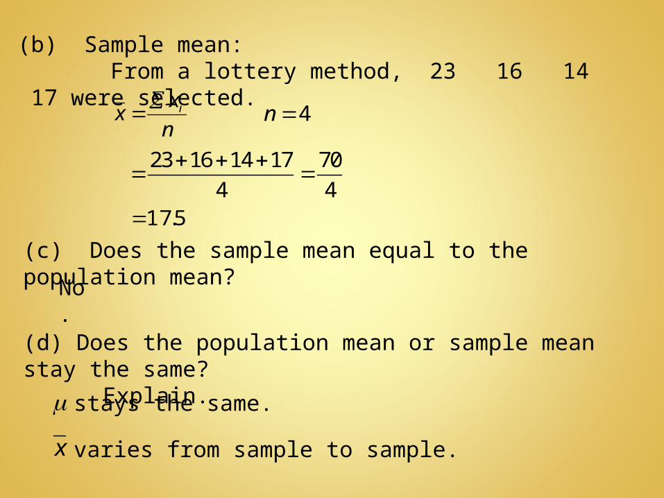
(b) Sample mean: From a lottery method, 23 16 14 17 were selected.
(c) Does the sample mean equal to the population mean?
No.
(d) Does the population mean or sample mean stay the same? Explain.
4nn
xx i
23 16 14 17 70
4 4
5.17
stays the same.
varies from sample to sample.x

If is odd, the median is the data value in the middle of the data
set; the location of the median is the position.
If is even, the median is the mean of the two middle
observations in the data set that lie in the and position
respectively.
A2. Median
The median, , is the value that lies in the middle of the data
when arranged in ascending order.
2
1n
M
n
n
12
n
2
n
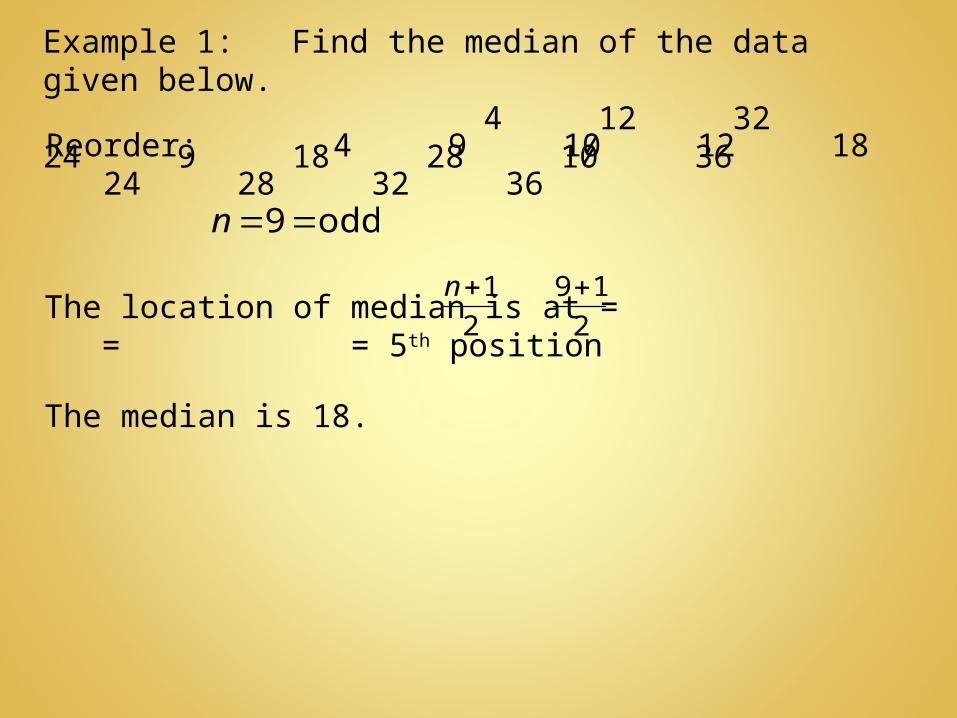
Example 1: Find the median of the data given below. 4 12 32 24 9 18 28 10 36
Reorder: 4 9 10 12 18 24 28 32 36
The median is 18.
odd9 n
The location of median is at = = = 5th position2
1n2
19

Example 2: Find the median of the data given below. $35.34 $42.09 $38.72 $43.28 $39.45 $49.36
$30.15 $40.88Reorder: $30.15 $35.34 $38.72 $39.45 $40.88 $42.09 $43.28 $49.36
The location of median is between and which is between
and = 4th and 5th position.
12
n
2
n
2
81
2
8
even8 n
The median 39.45 40.88 80.33
2 2
165.40
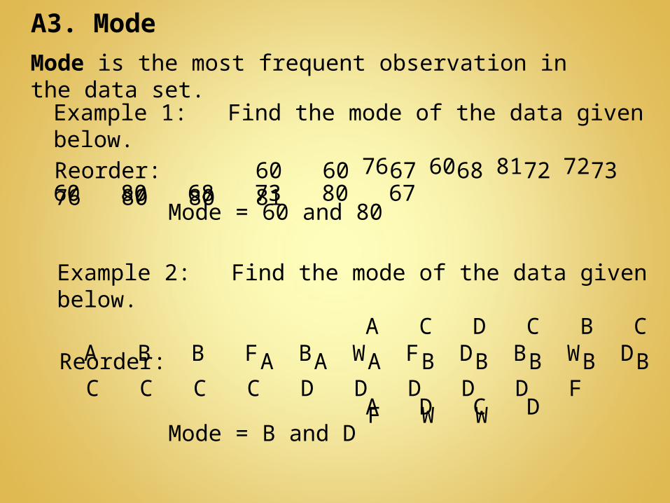
A3. ModeMode is the most frequent observation in the data set.
Example 1: Find the mode of the data given below. 76 60 81 72 60 80 68 73 80 67 Reorder: 60 60 67 68 72 73 76 80 80 81
Mode = 60 and 80
Example 2: Find the mode of the data given below. A C D C B C A B B F B W F D B W D A D C D
Reorder: A A A B B B B B C C C C D D D D D F F W W
Mode = B and D
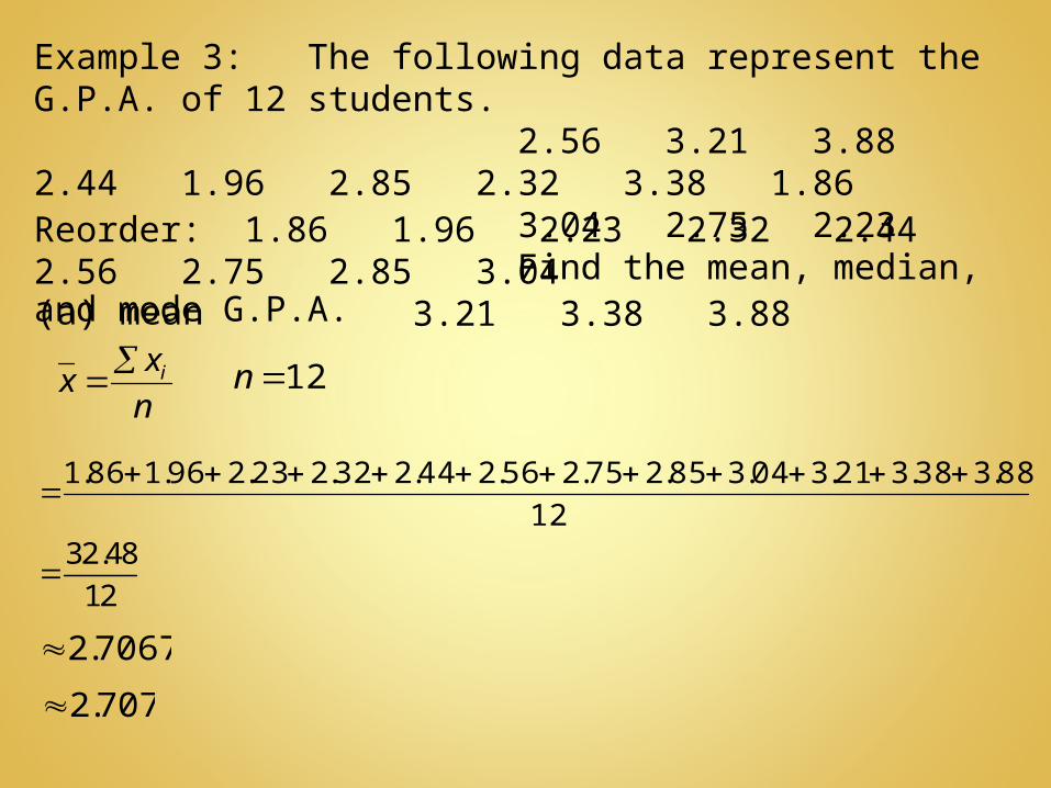
Example 3: The following data represent the G.P.A. of 12 students. 2.56 3.21 3.88 2.44 1.96 2.85 2.32 3.38 1.86 3.04 2.75 2.23 Find the mean, median, and mode G.P.A.Reorder: 1.86 1.96 2.23 2.32 2.44 2.56 2.75 2.85 3.04 3.21 3.38 3.88 (a) mean
12nn
xx i
12
88.338.321.304.385.275.256.244.232.223.296.186.1
7067.2
707.2
32.48
12

(b) median
(c) modeNone.
Reorder: 1.86 1.96 2.23 2.32 2.44 2.56 2.75 2.85 3.04 3.21 3.38 3.88 6th 7th
even12 n
The median
The location of median is between and which is between
and = 6th and 7th position.
12
12
2
n
2
12
12
n
655.22
31.5
2
75.256.2
Chapter 3.1 Measures of Central Tendency
Objective A : Mean, Median, and Mode
Objective B : Relation Between the Mean, Median, and Distribution Shape
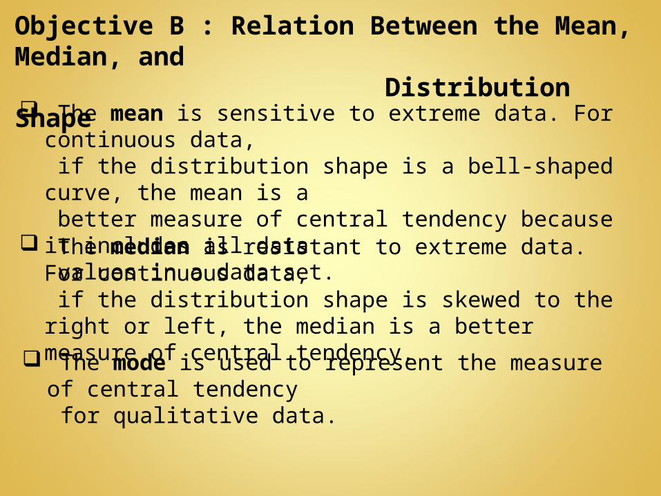
Objective B : Relation Between the Mean, Median, and Distribution Shape
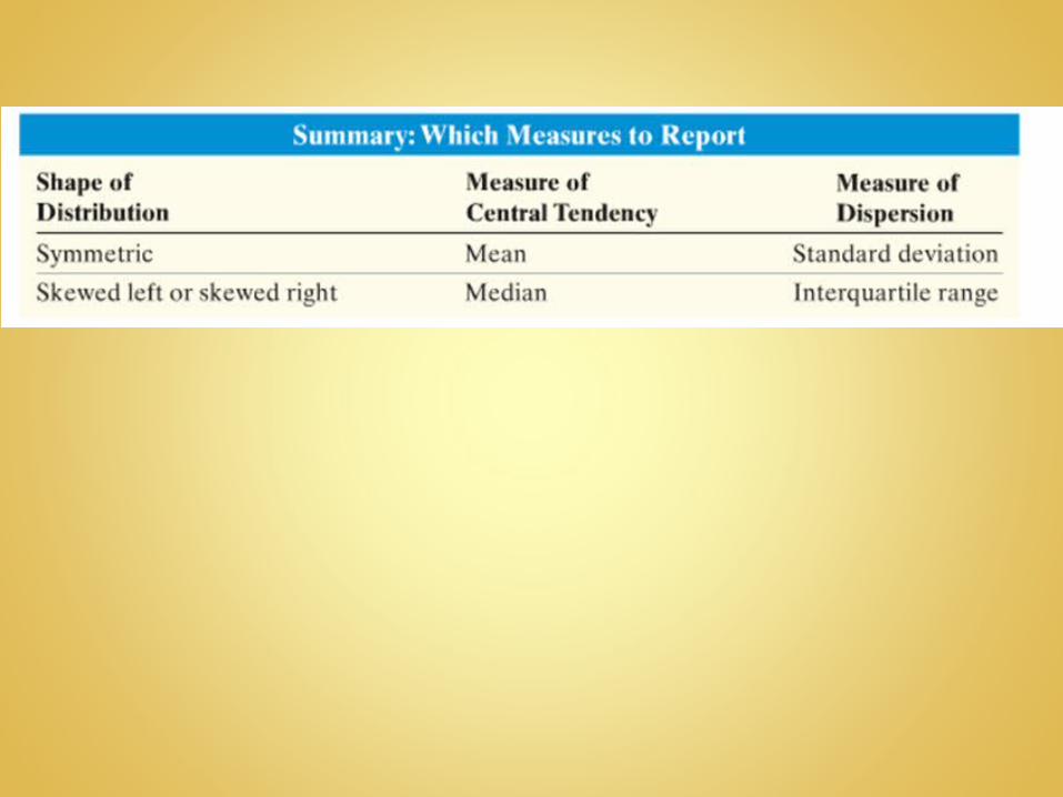
The mean is sensitive to extreme data. For continuous data, if the distribution shape is a bell-shaped curve, the mean is a better measure of central tendency because it includes all data values in a data set.
The median is resistant to extreme data. For continuous data, if the distribution shape is skewed to the right or left, the median is a better measure of central tendency.
The mode is used to represent the measure of central tendency for qualitative data.

Mean or Median versus Skewness

Chapter 3.2 Measures of Dispersion
Objective A : Range, Variance, and Standard Deviation
Objective B : Empirical Rule
Objective C : Chebyshev’s Inequality

Chapter 3.2 Measures of Dispersion (Part I)
Measurement of dispersion is a numerical measure that can quantify the spread of data.In this section, the three numerical measures of dispersion that we will discuss are the range, variance, and standard deviation. In the later section, we will discuss another measure of dispersion called interquartile range (IQR).
A1. Range Range = = largest data value – smallest data valueThe range is not resistant because it is affected by extreme
values in the data set.
R
Objective A : Range, Variance, and Standard Deviation

Definition Formula
A2. Variance and Standard Deviation
Standard Deviation is based on the deviation about the mean. Since the sum of deviation about the mean is zero, we cannot use the average deviation about the mean as a measure of spread.
We use the average squared deviation (variance) instead.
The population variance, , of a variable is the sum of the squared deviations about the population mean, , divided by the number of observations in the population, .
Computational Formula
N
xi2
2 )(
N
NNx
x ii
22
2
)(
2
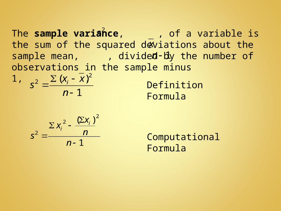
The sample variance, , of a variable is the sum of the squared deviations about the sample mean, , divided by the number of observations in the sample minus 1, .
Definition Formula
Computational Formula
2sx
1n
1
)( 22
n
xxs i
1
)( 22
2
nnx
xs
ii

In order to use the sample variance to obtain an unbiased estimate of the population variance, we divide the sum of the squared deviations about the sample mean by . We call the degree of freedom because the first observations have freedom to be whatever value they wish, but the th value has no freedom in order to force to be zero.
n
The sample standard deviation, , is the square root of the sample variance or .
The population standard deviation, , is the square root of the population variance or .
To avoid round-off error, never use the rounded value of the variance to compute the standard deviation. Keep a few more decimal places for an intermediate step calculation.
1n 1n1n
)( xxi
variancepopulation
variancesampless
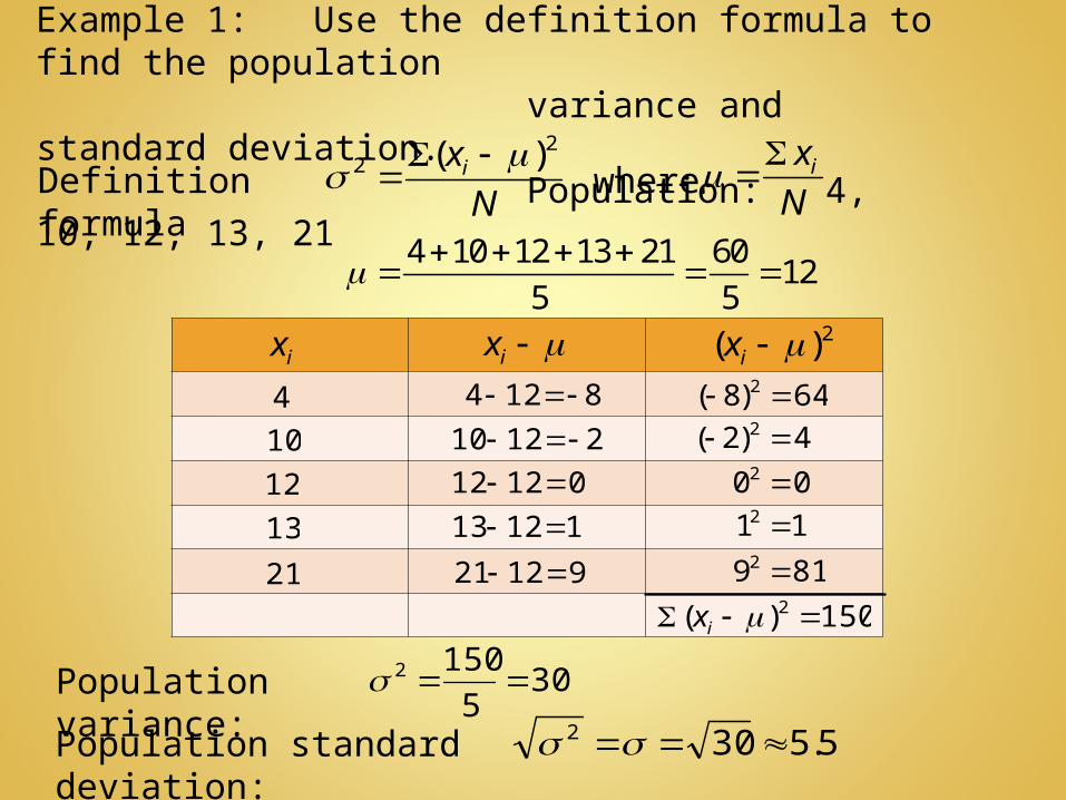
Example 1: Use the definition formula to find the population variance and standard deviation. Population: 4, 10, 12, 13, 21
Definition formula whereN
xi2
2 )(
N
xi
4 10 12 13 21 6012
5 5
Population variance: 305
1502
Population standard deviation: 5.5302
8124 64)8( 2 21210 4)2( 2
01212 002 11213 112
91221 8192
4
10
12
13
21
ix ix2)( ix
150)( 2 ix

Example 2: Use the definition formula to find the sample variance and standard deviation.
Sample: 83, 65, 91, 84
Definition formula where1
)( 22
n
xxs i
n
xx i
Sample variance: 9.1229166.12214
75.3682
s
Sample standard deviation: 1.1108677.119166.122 s
83 65 91 84 32380.75
4 4x
Sample mean:
25.275.8083 0625.5)25.2( 2 75.1575.8065 0625.248)75.15( 2
25.1075.8091 0625.105)25.10( 2 25.375.8084 5625.10)25.3( 2
83
65
91
84
ix xxi 2)( xxi
75.368)( 2 xxi
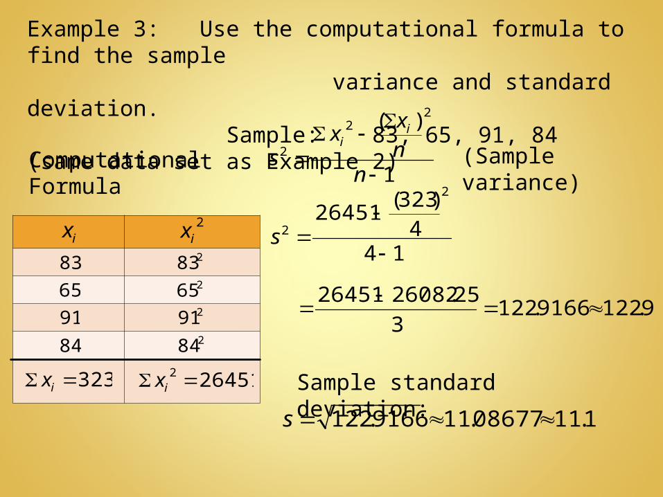
Example 3: Use the computational formula to find the sample variance and standard deviation.
Sample: 83, 65, 91, 84 (same data set as Example 2)
Computational Formula (Sample variance) 1
)( 22
2
nnx
xs
ii
144
)323(26451
2
2
s
9.1229166.1223
25.2608226451
Sample standard deviation:
1.1108677.119166.122 s
83 283
65 265
91 291
84 284
ix2ix
323 ix 264512 ix
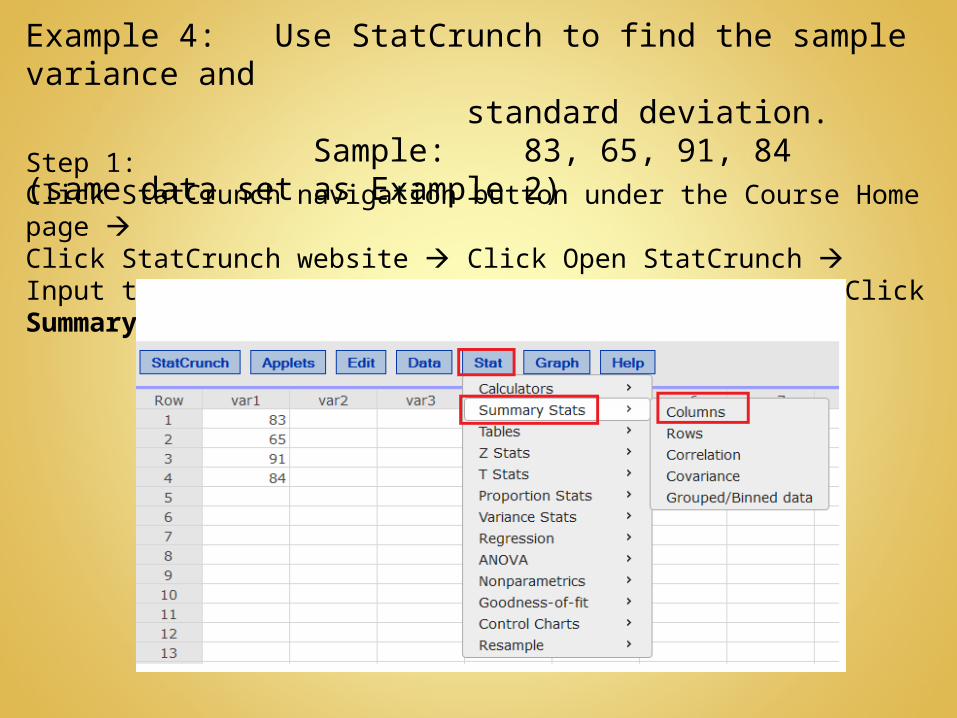
Example 4: Use StatCrunch to find the sample variance and standard deviation.
Sample: 83, 65, 91, 84 (same data set as Example 2)
Step 1:Click StatCrunch navigation button under the Course Home page Click StatCrunch website Click Open StatCrunch Input the raw data in Var 1 column Click Stat Click Summary Stats Columns
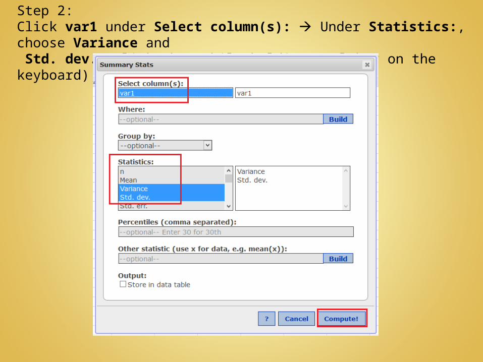
Step 2:Click var1 under Select column(s): Under Statistics:, choose Variance and Std. dev. (click them while holding Ctrl key on the keyboard) Click Compute!
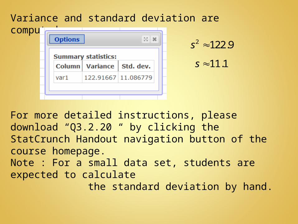
Note : For a small data set, students are expected to calculate the standard deviation by hand.
Variance and standard deviation are computed.
2 122.9s
11.1s
For more detailed instructions, please download “Q3.2.20 “ by clicking the StatCrunch Handout navigation button of the course homepage.
Chapter 3.2 Measures of Dispersion
Objective A : Range, Variance, and Standard Deviation
Objective B : Empirical Rule
Objective C : Chebyshev’s Inequality

Objective B : Empirical Rule

The figure below illustrates the Empirical Rule.
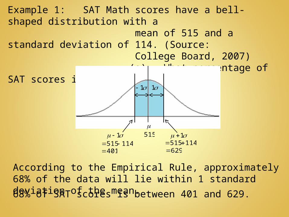
Example 1: SAT Math scores have a bell-shaped distribution with a mean of 515 and a standard deviation of 114. (Source: College Board, 2007) (a) What percentage of SAT scores is between 401 and 629?
According to the Empirical Rule, approximately 68% of the data will lie within 1 standard deviation of the mean.
68% of SAT scores is between 401 and 629.
1 1
114515 401
114515629
515 1 1
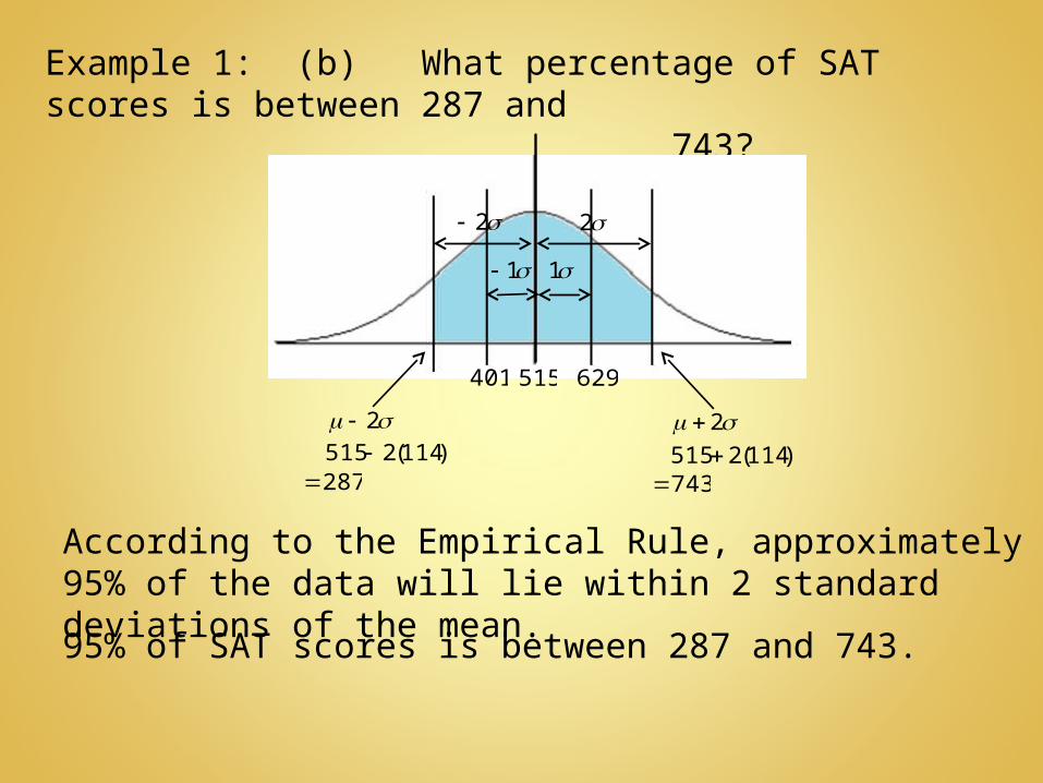
Example 1: (b) What percentage of SAT scores is between 287 and 743?
According to the Empirical Rule, approximately 95% of the data will lie within 2 standard deviations of the mean.
95% of SAT scores is between 287 and 743.
1 1
515
)114(2515743
)114(2515 287
2 2
401 629
2 2

Example 1: (c) What percentage of SAT scores is less than 401 or greater than 629?
– %100 %68
= 1 1
515401 629
%32
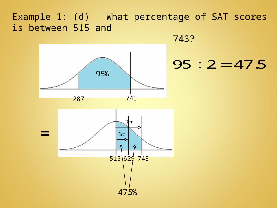
Example 1: (d) What percentage of SAT scores is between 515 and 743?
= 1
2
515 629 743
%5.47
95 2 47.5 %95
743287
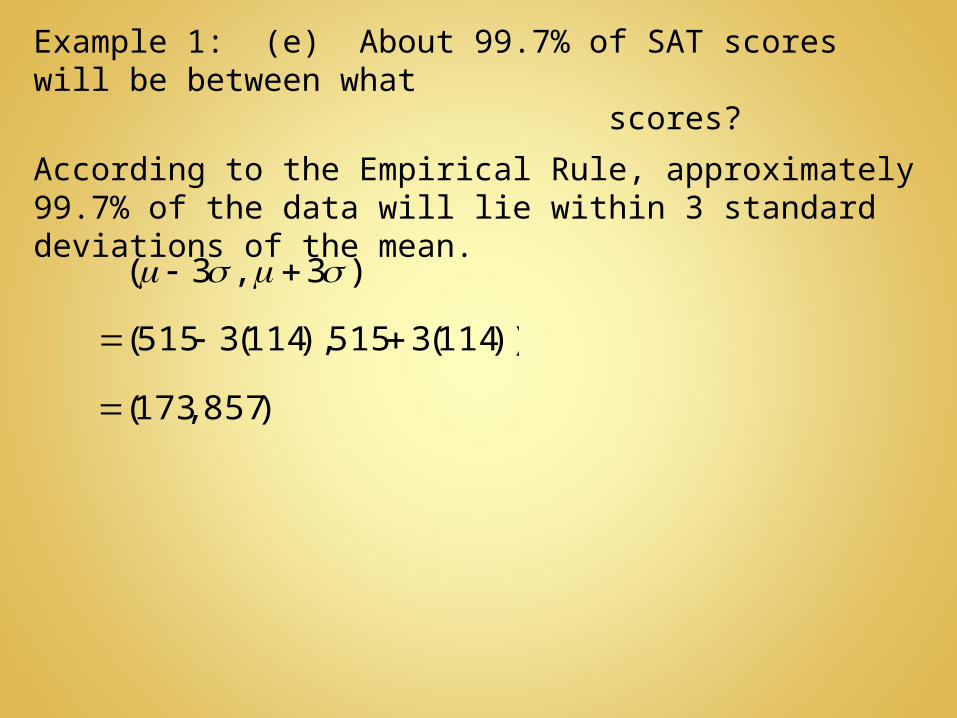
Example 1: (e) About 99.7% of SAT scores will be between what scores?
According to the Empirical Rule, approximately 99.7% of the data will lie within 3 standard deviations of the mean.
)3,3(
))114(3515),114(3515(
)857,173(

Chapter 3.2 Measures of Dispersion
Objective A : Range, Variance, and Standard Deviation
Objective B : Empirical Rule
Objective C : Chebyshev’s Inequality

Objective C : Chebyshev’s Inequality

Example 1: According to the U.S. Census Bureau, the mean of the commute time to for a resident to Boston, Massachusetts, is 27.3 minutes. Assume that the standard deviation of the commute time is 8.1 minutes to answer the following:(a)What minimum percentage of commuters in Boston has a commute time within 2 standard deviations of the mean?
According to the Chebyshev’s Inequality, at least
will lie within 2 standard deviations of the mean.
%100)1
1(2k
Standard deviation → 2k
%100)2
11(
2 %100)
4
11( %75

Example 1: (b) (i) What minimum percentage of commuters in Boston has a commute time within 1.5 standard deviations of the mean? (ii) What are the commute times within 1.5 standard deviations of the mean?
At least 55.6% of commuters in Boston has a commute time between 15.15 minutes and 39.45 minutes
55.6% of commuters in Boston has a commute time.
(i) According to the Chebyshev’s Inequality, at least
of the data will lie within standard deviations of the mean.
Since ,
%100)1
1(2
k
k
5.1k %6.55%100...)4444.01(%100)5.1
11(
2
(ii) ( 1.5 , 1.5 ) (27.3 1.5(8.1), 27.3 1.5(8.1)) (15.15, 39.45)

Chapter 3.3Measures of Central Tendency and Dispersion from Grouped Data
In this section we are going to learn how to calculate the mean, , and the weighted mean, , from data that have already been summarized in frequency distributions (group data).
Midpoint = (Adding consecutive lower class limits) ÷ 2
Since raw data cannot be retrieved from a frequency table, the class midpoint is used to represent the mean of the data values within each class.
x
wx
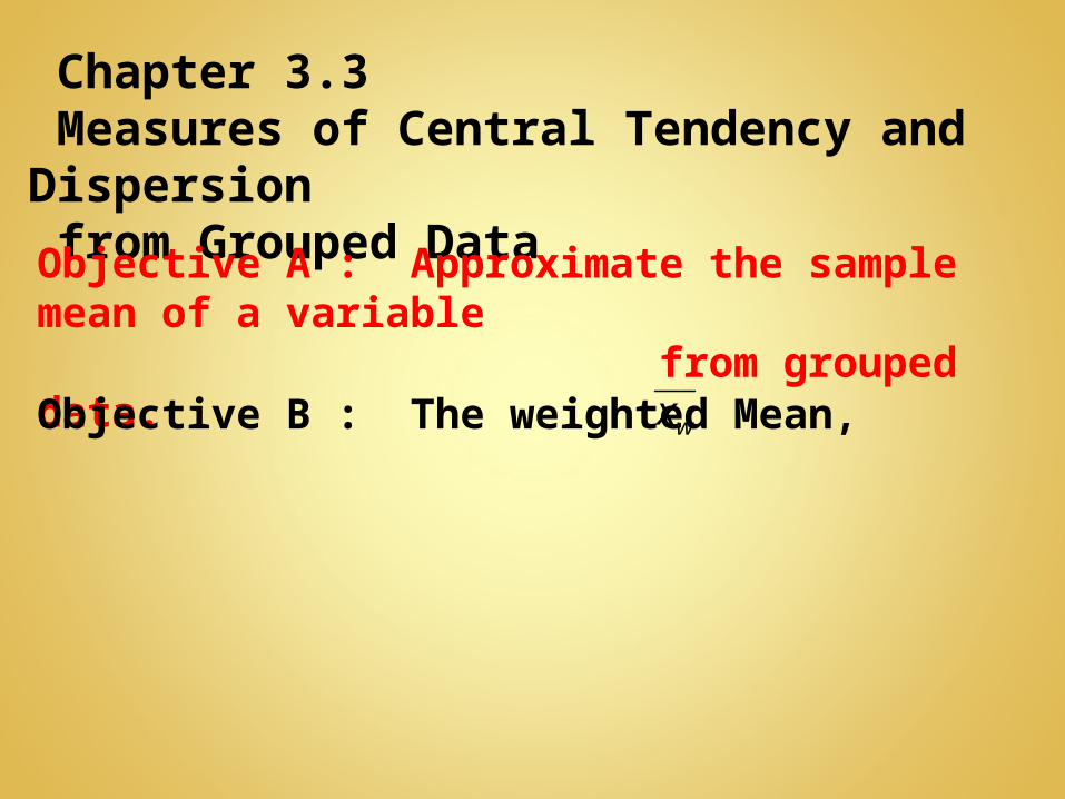
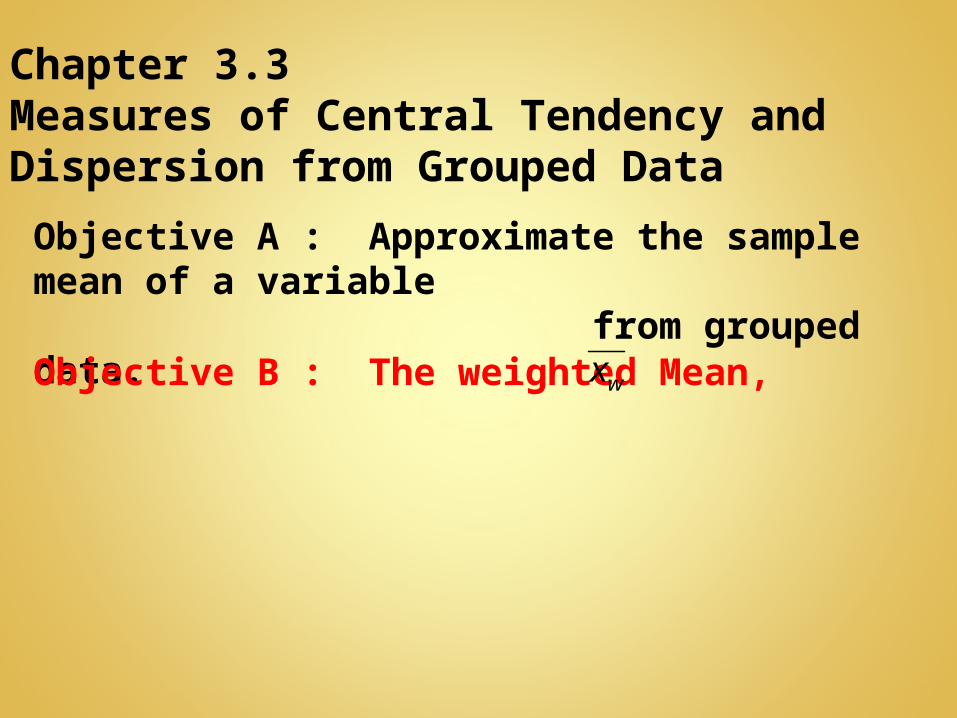
Chapter 3.3 Measures of Central Tendency and Dispersion from Grouped Data
Objective A : Approximate the sample mean of a variable from grouped data.
Objective B : The weighted Mean, wx
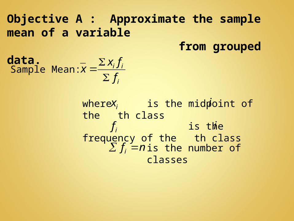
Objective A : Approximate the sample mean of a variable from grouped data.
Sample Mean:
is the frequency of the th class
where is the midpoint of the th class
is the number of classes
i
i
ix
i
ii
f
fxx
if
nfi
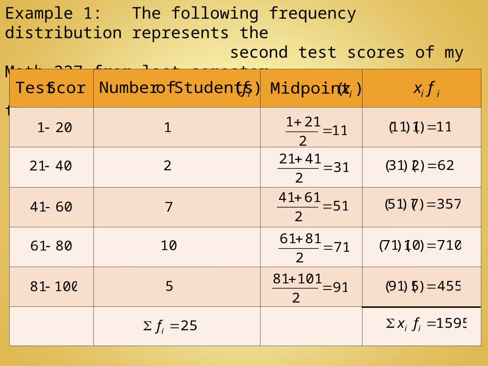
Example 1: The following frequency distribution represents the second test scores of my Math 227 from last semester. Approximate the mean of the score.
1 11)1)(11( 112
211
201
4021 312
4121
62)2)(31( 2
6041 512
6141
357)7)(51( 7
8061 712
8161
710)10)(71( 10
10081 912
10181
455)5)(91( 5
ScoreTest )(StudentsofNumber if )(Midpoint ix ii fx
25 if 1595 ii fx
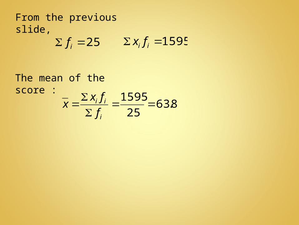
The mean of the score :
8.6325
1595
i
ii
f
fxx
From the previous slide,
25 if 1595 ii fx
Chapter 3.3Measures of Central Tendency and Dispersion from Grouped Data
Objective A : Approximate the sample mean of a variable from grouped data.
Objective B : The weighted Mean, wx

Objective B : The weighted Mean,
We compute the weighted mean when data values are not weighted equally.
where is the weight of the th observation
is the value of the th observation
i iw
i
w xx
w
i
iiw
ix
wx
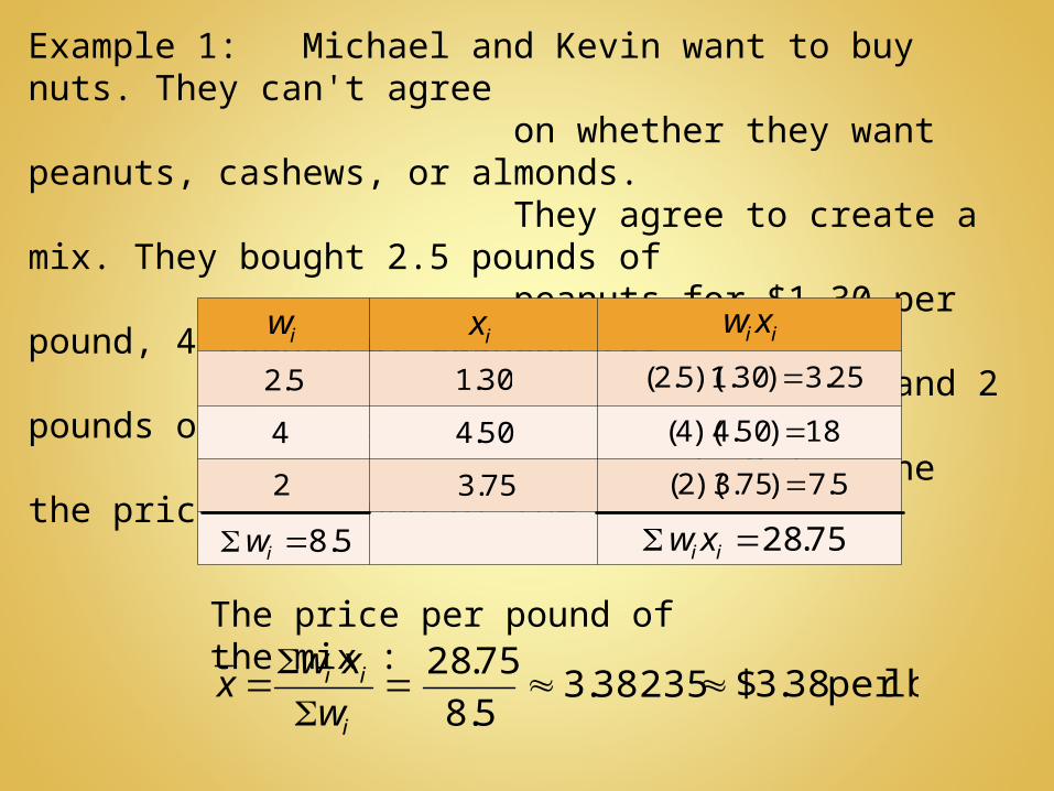
Example 1: Michael and Kevin want to buy nuts. They can't agree on whether they want peanuts, cashews, or almonds. They agree to create a mix. They bought 2.5 pounds of peanuts for $1.30 per pound, 4 pounds of cashews for $4.50 per pounds, and 2 pounds of almonds for $3.75 per pound. Determine the price per pound of the mix.
The price per pound of the mix :
5.2 30.1 25.3)30.1)(5.2(
4 50.4 18)50.4)(4(
2 75.3 5.7)75.3)(2(
iw ix iixw
75.28 iixw5.8 iw
i
ii
w
xwx
5.8
75.2838235.3 lbper38.3$
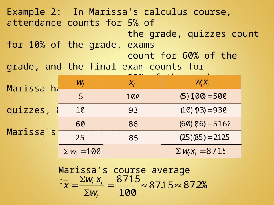
Example 2: In Marissa's calculus course, attendance counts for 5% of
the grade, quizzes count for 10% of the grade, exams count for 60% of the grade, and the final exam counts for 25% of the grade. Marissa had a 100% average for attendance, 93% for quizzes, 86% for exams, and 85% on
the final. Determine Marissa's course average.
Marissa’s course average :
5 100 500)100)(5(
10 93 930)93)(10(
60 86 5160)86)(60(
iw ix iixw
25 85 (25)(85) 2125
8715 iixw100 iw
i
ii
w
xwx
100
871515.87 %2.87
Ch 3.4 Measures of Positions and Outliers
Objective A : -scoresz
Objective B : Percentiles and Quartiles
Objective C : Outliers

Ch3.4 Measures of Positions and Outliers
Objective A : -scores
The -score represents the distance that a data value is from the mean in terms of the number of standard deviations.
Population -score:
Sample -score:
x
z
z
s
xxz
z
z
z
Measures of position determine the relative position of a certain data value within the entire set of data.
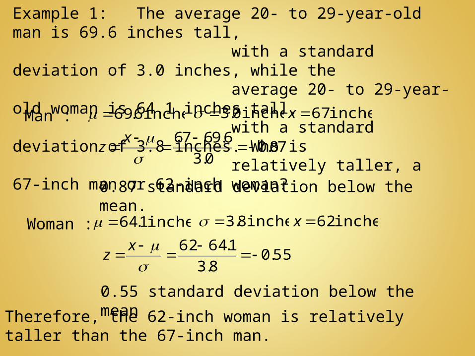
Example 1: The average 20- to 29-year-old man is 69.6 inches tall, with a standard deviation of 3.0 inches, while the average 20- to 29-year-old woman is 64.1 inches tall, with a standard deviation of 3.8 inches. Who is relatively taller, a 67-inch man or 62-inch woman?
0.87 standard deviation below the mean.
0.55 standard deviation below the mean
Therefore, the 62-inch woman is relatively taller than the 67-inch man.
67 69.60.87
3.0
xz
Man : inches6.69 inches0.3 inches67x
Woman : inches1.64 inches8.3 inches62x
55.08.3
1.6462
x
z
Ch 3.4 Measures of Positions and Outliers
Objective A : -scoresz
Objective B : Percentiles and Quartiles
Objective C : Outliers

Objective B : Percentiles and Quartiles
The th percentile, , of a set of data is a value such that percent of the observations are less than or equal to the value.
kPk k
Example 1: Explain the meaning of the 5th percentile of the weight of males 36 months of age is 12.0 kg.
5% of 36-month-old males weighs 12.0 kg or less.95% of 36-month-old males weighs more than 12.0 kg.
B1. Percentiles

The second quartile, , is equivalent to .
The most common percentiles are quartiles.
The first quartile, , is equivalent to .
The third quartile, , is equivalent to .
25P1Q
2Q
3Q
50P
75P

Example 2: Determine the quartiles of the following data. 46 45 58 71 42 66 72 42 61 49 80
Lower half of the data : 42 42 45 46 49
451 Q
Ascending order : 42 42 45 46 49 58 61 66 71 72 80
58M582 Q
Upper half of the data : 61 66 71 72 80
713 Q

The interquartile range, IQR, is the measure of dispersion that is based on quartiles. The range and standard deviation are effected by extreme values. The IQR is resistant to extreme values.
B2. Interquartile

Example 1: One variable that is measured by online homework systems is the amount of time a student spends on homework for each section of the text. The following is a summary of the number of minutes a student spends for each section of the text for the fall 2007 semester in
a College Algebra class at Joliet Junior College.(a) Provide an interpretation of these results.
421 Q 5.723 Q5.512 Q
25% of the students spend 42 minutes or less on homework for each section, and 75% of the students spend more than 42 minutes.
:421 Q
50% of the students spend 51.5 minutes or less on homework for each section, and 50% of the students spend more than 51.5 minutes.
:5.512 Q
75% of the students spend 72.5 minutes or less on homework for each section, and 25% of the students spend more than 72.5 minutes.
:5.723 Q

(b) Determine and interpret the interquartile range.
(c) Do you believe that the distribution of time spent doing homework is skewed or symmetric? Why?
The middle of 50% of all students has a range of 30.5 minutes of time spent on homework.
minutes5.30425.7213 QQIQR
Skewed right. The difference between and is less than the difference between and .
2Q
2Q1Q
3Q
Ch 3.4 Measures of Positions and Outliers
Objective A : -scoresz
Objective B : Percentiles and Quartiles
Objective C : Outliers

Extreme observations are called outliers; they may occur by error in the measurement or during data entry or from errors in sampling.
Objective C : Outliers
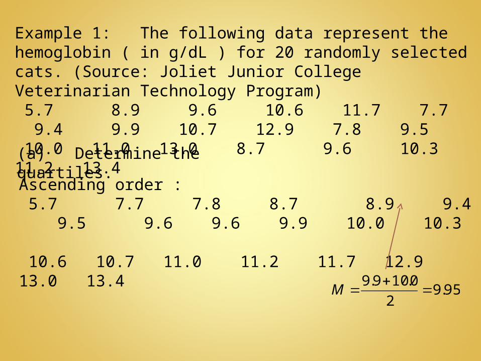
Example 1: The following data represent the hemoglobin ( in g/dL ) for 20 randomly selected cats. (Source: Joliet Junior College Veterinarian Technology Program) 5.7 8.9 9.6 10.6 11.7 7.7 9.4 9.9 10.7 12.9 7.8 9.5 10.0 11.0 13.0 8.7 9.6 10.3 11.2 13.4(a) Determine the quartiles.
Ascending order : 5.7 7.7 7.8 8.7 8.9 9.4 9.5 9.6 9.6 9.9 10.0 10.3 10.6 10.7 11.0 11.2 11.7 12.9 13.0 13.4
95.92
0.109.9
M
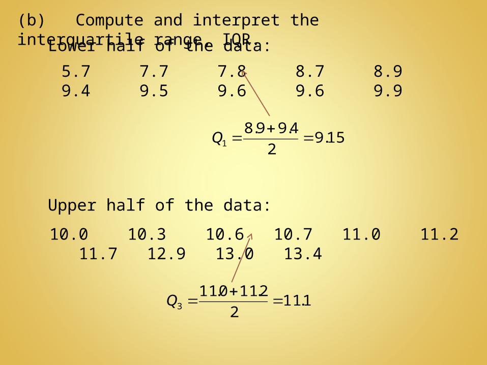
(b) Compute and interpret the interquartile range, IQR.
Lower half of the data:
5.7 7.7 7.8 8.7 8.9 9.4 9.5 9.6 9.6 9.9
15.92
4.99.81
Q
10.0 10.3 10.6 10.7 11.0 11.2 11.7 12.9 13.0 13.4
Upper half of the data:
1.112
2.110.113
Q
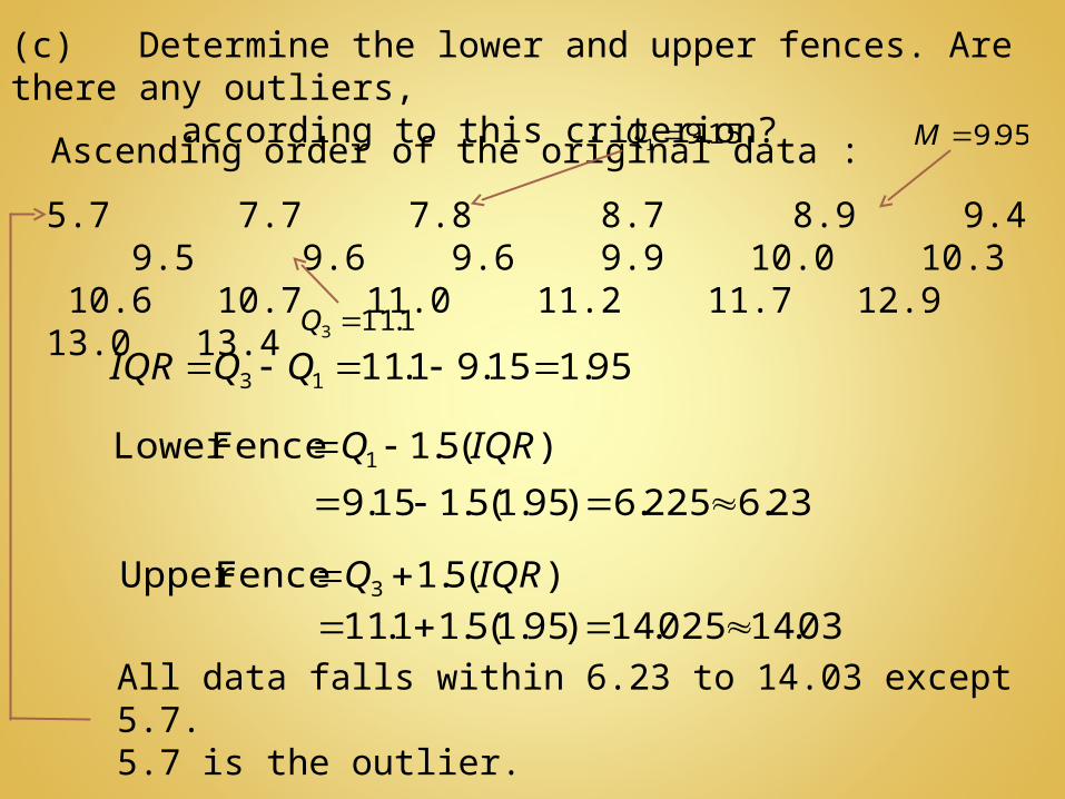
(c) Determine the lower and upper fences. Are there any outliers, according to this criterion?
All data falls within 6.23 to 14.03 except 5.7.5.7 is the outlier.
95.115.91.1113 QQIQR
)(5.1FenceLower 1 IQRQ
)(5.1FenceUpper 3 IQRQ
23.6225.6)95.1(5.115.9
03.14025.14)95.1(5.11.11
Ascending order of the original data :
5.7 7.7 7.8 8.7 8.9 9.4 9.5 9.6 9.6 9.9 10.0 10.3 10.6 10.7 11.0 11.2 11.7 12.9 13.0 13.4
15.91 Q
1.113 Q
95.9M
Objective A : The Five-Number Summary
Ch 3.5 The Five-Number Summary and Boxplots
Objective B : Boxplots
Objective C : Using a Boxplot to describe the shape of a distribution
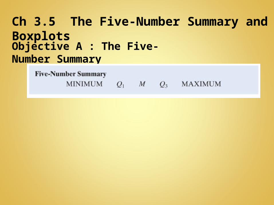
Objective A : The Five-Number Summary
Ch 3.5 The Five-Number Summary and Boxplots
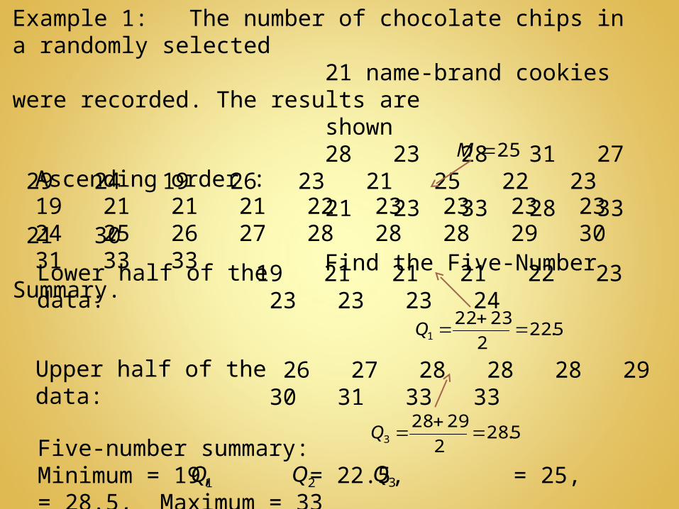
Example 1: The number of chocolate chips in a randomly selected 21 name-brand cookies were recorded. The results are shown 28 23 28 31 27 29 24 19 26 23 21 25 22 23 21 23 33 28 33 21 30 Find the Five-Number Summary.Ascending order :
19 21 21 21 22 23 23 23 23 24 25 26 27 28 28 28 29 30 31 33 33
25M
Lower half of the data: 19 21 21 21 22 23 23 23 23 24
5.222
23221
Q
Upper half of the data: 26 27 28 28 28 29 30 31 33 33
5.282
29283
Q
Five-number summary:Minimum = 19, = 22.5, = 25, = 28.5, Maximum = 33 1Q 3Q2Q

Objective A : The Five-Number Summary
Ch 3.5 The Five-Number Summary and Boxplots
Objective B : Boxplots
Objective C : Using a Boxplot to describe the shape of a distribution
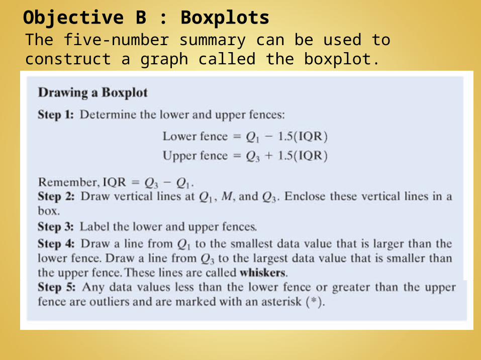
Objective B : BoxplotsThe five-number summary can be used to construct a graph called the boxplot.
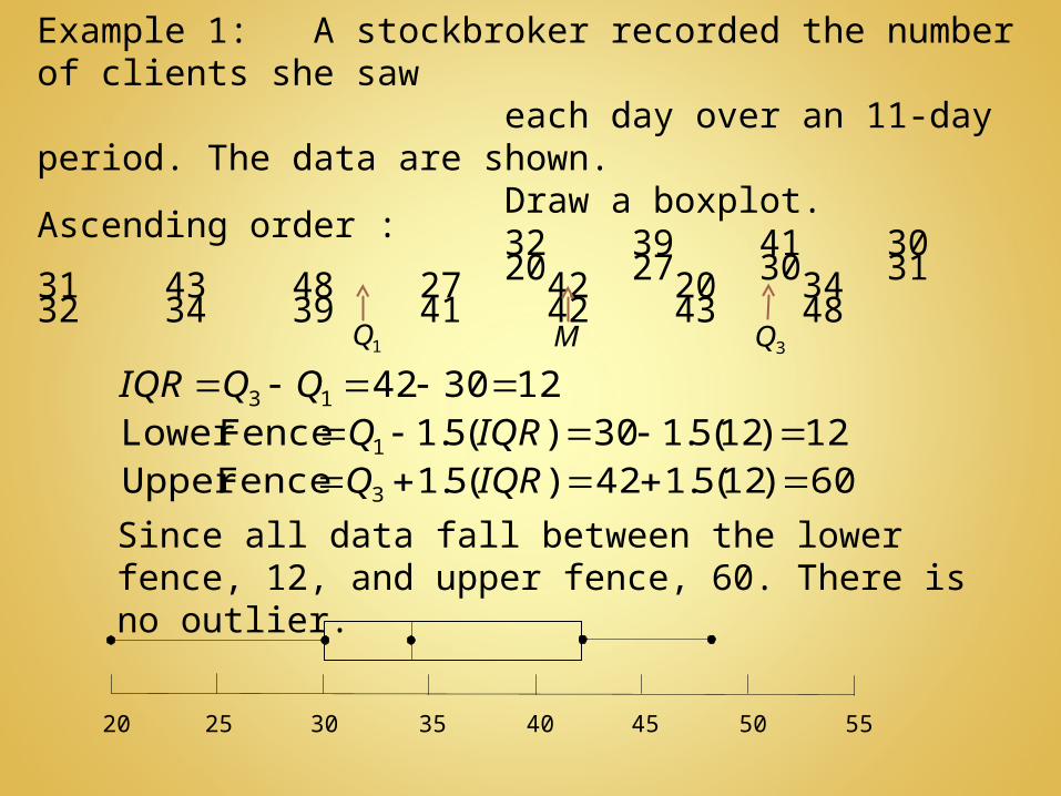
Example 1: A stockbroker recorded the number of clients she saw each day over an 11-day period. The data are shown. Draw a boxplot. 32 39 41 30 31 43 48 27 42 20 34
Since all data fall between the lower fence, 12, and upper fence, 60. There is no outlier.
20 25 30 35 40 5045 55
Ascending order : 20 27 30 31 32 34 39 41 42 43 48
M1Q 3Q
12304213 QQIQR12)12(5.130)(5.1FenceLower 1 IQRQ60)12(5.142)(5.1FenceUpper 3 IQRQ

Objective A : The Five-Number Summary
Ch 3.5 The Five-Number Summary and Boxplots
Objective B : Boxplots
Objective C : Using a Boxplot to describe the shape of a distribution

Objective C : Using a Boxplot to describe the shape of a distribution

Example 1: Use the side-by-side boxplots shown to answer the questions that follow.
(a) To the nearest integer, what is the median of variable ?
(b) To the nearest integer, what is the first quartile of variable ?
x
y
15
22
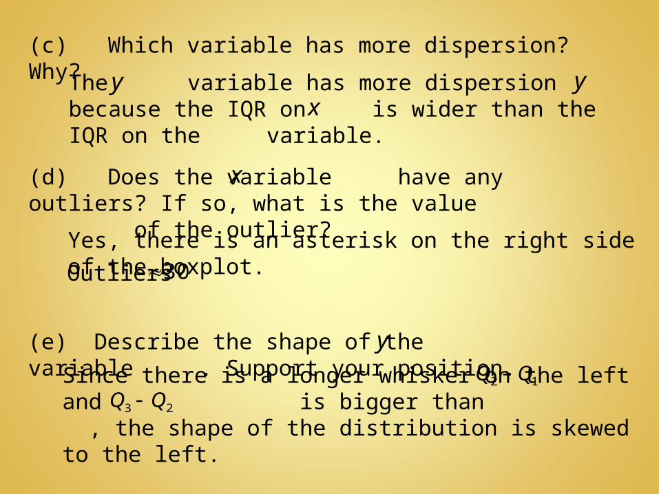
(e) Describe the shape of the variable . Support your position.
(c) Which variable has more dispersion? Why?
(d) Does the variable have any outliers? If so, what is the value of the outlier?
y
x
The variable has more dispersion because the IQR on is wider than the IQR on the variable.
y yx
Yes, there is an asterisk on the right side of the boxplot.Outliers 30
Since there is a longer whisker on the left and is bigger than , the shape of the distribution is skewed to the left.
12 QQ
23 QQ
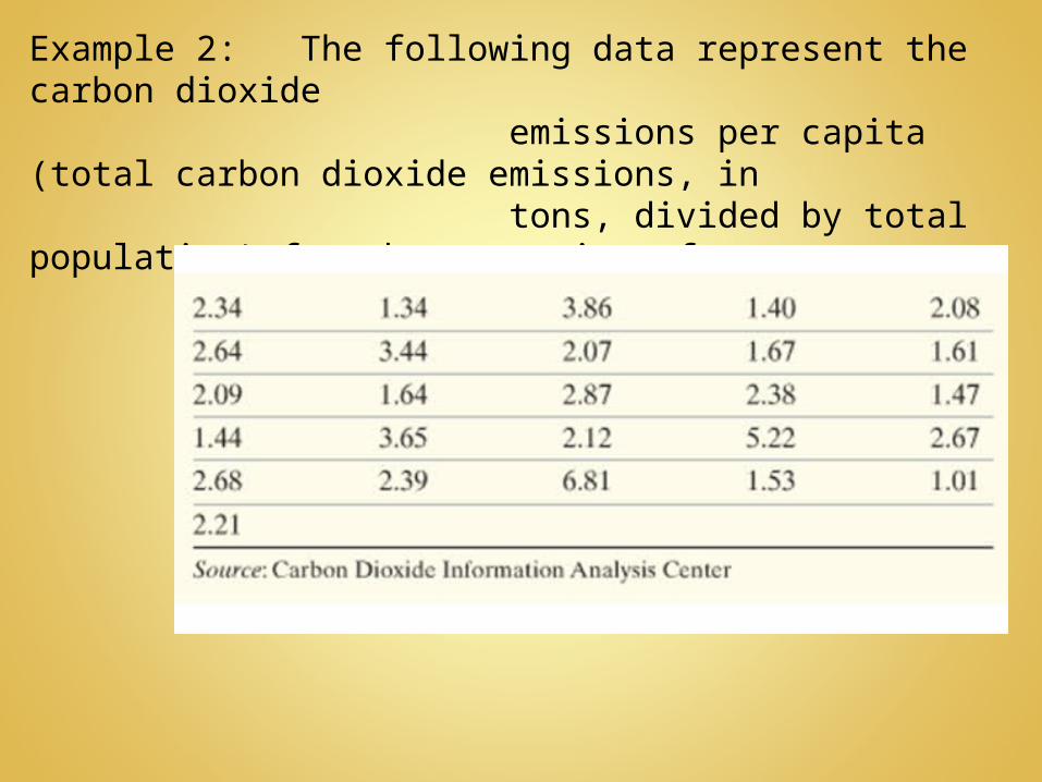
Example 2: The following data represent the carbon dioxide emissions per capita (total carbon dioxide emissions, in tons, divided by total population) for the countries of Western Europe in 2004.
(b) Determine the lower and upper fences.
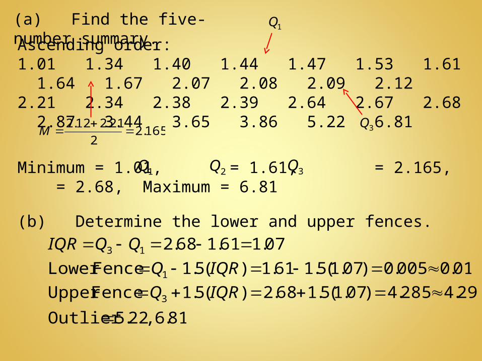
(a) Find the five-number summary.
Ascending order: 1.01 1.34 1.40 1.44 1.47 1.53 1.61 1.64 1.67 2.07 2.08 2.09 2.12 2.21 2.34 2.38 2.39 2.64 2.67 2.68 2.87 3.44 3.65 3.86 5.22 6.81
165.22
21.212.2
M
1Q
3Q
07.161.168.213 QQIQR
01.0005.0)07.1(5.161.1)(5.1FenceLower 1 IQRQ
29.4285.4)07.1(5.168.2)(5.1FenceUpper 3 IQRQ
81.6,22.5Outlier
Minimum = 1.01, = 1.61, = 2.165, = 2.68, Maximum = 6.81 1Q 3Q2Q
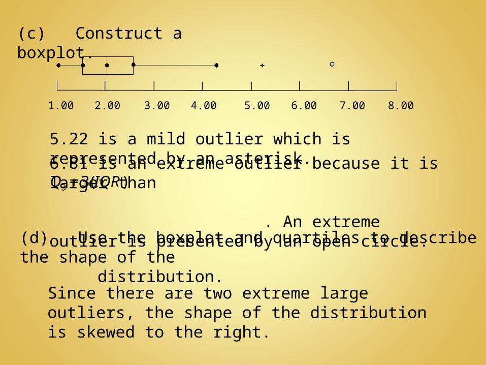
Since there are two extreme large outliers, the shape of the distribution is skewed to the right.
(c) Construct a boxplot.
1.00 2.00 3.00 4.00 5.00 7.006.00 8.00
5.22 is a mild outlier which is represented by an asterisk.
(d) Use the boxplot and quartiles to describe the shape of the distribution.
6.81 is an extreme outlier because it is larger than . An extreme outlier is presented by an open circle.
)(33 IQRQ

Note: Part (a) and (c) can be easily done by using StatCrunch. For the instructions, please refer to the StatCrunch handout.
Related Documents