Suite - DiVA-Portal

Master of Science Thesis

Department of Energy Technology

KTH 2021

Coolant Filling Simulation Model in 1D with GT-

Suite

TRITA: TRITA-ITM-EX 2021:492

Kapil Vaidya

Xavier Navarro Palau

Approved

2021-08-26

Examiner

Justin Chiu

Supervisor

Justin Chiu

Industrial Supervisor

Harun Poljo

Contact person

Harun Poljo

Abstract

Driven by the goal of decreasing emissions and pollutants towards a more sustainable future,

the automotive industry is undergoing a rapid transition towards battery-powered electric

vehicles. This shift to sustainable transport is fast-paced, and new technical solutions are being

offered on a regular basis to fulfil the future needs for electric vehicles, including battery-

electric trucks. This continuously necessitates a fast development of the battery-electric truck,

along with the cooling system. To validate the cooling system, Scania's preferred approaches

are testing and 3D simulations. However, these approaches are time-consuming and cannot

match the pace of the design or the development.

This thesis addresses the implementation of using 1D Simulations (GT-Suite) to carry out

coolant filling simulations as a more efficient approach by studying the filling of the battery

cooling system in an electric truck and, later, validating the results obtained with a test rig. In

this thesis, different cases were defined, each adding more complexity to the circuit, and the

parameters studied were the filling times and the location of air traps. Finally, a case with a

closed circuit and running a coolant pump was developed to study the possibilities of devising

quicker deaeration techniques for the circuit.

The work completed in this thesis may be used as an example of how filling simulations can be

performed with GT-Suite. This thesis is a good starting point, exploring a vast potential in using

1D Simulations to simulate the coolant-air interaction in a cooling system. Nonetheless, the

findings revealed that GT-Suite v2020 and v2021 lack a robust model to properly simulate the

interaction of coolant and air in certain sections of the circuit. In addition, the simulation model

failed to obtain a steady-state solution in some cases resulting in discrepancies between the

results from the test rig and the simulations.

In conclusion, it was found that 1D simulations are not an ideal way forward when individual

components of the cooling circuit are being considered, for example, the cooling plates, but are

much quicker and seem to be a promising method to get an overview on a system level.

Keywords: GT-Suite, CFD, 1D Simulations, Battery cooling, BEV Truck, Deaeration, Air

Traps

Sammanfattning

Fordonsindustrin drivs av målet att minska utsläppen och föroreningarna mot en mer hållbar

framtid och genomgår en snabb omställning mot batteridrivna elfordon. Övergången till

hållbara transporter går snabbt och nya tekniska lösningar erbjuds regelbundet för att möta de

framtida behoven av elfordon, inklusive batteridrivna lastbilar. Detta kräver kontinuerligt en

snabb utveckling av den batteri-elektriska lastbilen, tillsammans med kylsystemet. För att

validera kylsystemet är Scanias föredragna metoder testning och 3D-simuleringar. Dessa

tillvägagångssätt är dock tidskrävande och kan inte matcha takten i designen eller utvecklingen.

Denna avhandling behandlar implementeringen av att använda 1D-simuleringar (GT-Suite) för

att utföra kylvätskefyllningssimuleringar som ett effektivare tillvägagångssätt genom att

studera fyllningen av batterikylsystemet i en elektrisk lastbil och senare validera resultaten som

erhållits med en testrigg. I denna avhandling definierades olika fall, var och en lägga till mer

komplexitet till kretsen, och de undersökta parametrarna var påfyllningstiderna och platsen för

luftfällor. Slutligen utvecklades ett fall med en sluten krets och kör en kylvätskepump för att

studera möjligheterna att utforma snabbare deaerationstekniker för kretsen.

Arbetet i denna avhandling kan användas som ett exempel på hur fyllningssimuleringar kan

utföras med GT-Suite. Denna avhandling är en bra utgångspunkt och utforskar en enorm

potential i att använda 1D-simuleringar för att simulera kylvätske-luftinteraktionen i ett

kylsystem. Resultaten visade dock att GT-Suite v2020 och v2021 saknar en robust modell för

att korrekt simulera interaktionen mellan kylvätska och luft i vissa delar av kretsen. Dessutom

kunde simuleringsmodellen inte få en steady state-lösning i vissa fall vilket resulterade i

skillnader mellan resultaten från testriggen och simuleringarna.

Sammanfattningsvis konstaterades det att 1D-simuleringar inte är en idealisk väg framåt när

enskilda komponenter i kylkretsen övervägs, till exempel kylplattorna, men är mycket snabbare

och verkar vara en lovande metod för att få en översikt på systemnivå.

Nyckelord: GT-Suite, CFD, 1D-simuleringar, Batterikylning, BEV Truck, Deaeration, Air

Traps

Acknowledgement

We would like to express our sincere gratitude to everyone who has helped us through this

master thesis.

First and foremost, we would like to thank Harun Poljo, our supervisor at Scania CV AB, for

his patience and guidance throughout the thesis work. We would also like to thank Magnus

Hultén, our manager at Scania CV AB, for ensuring that we had all the necessary resources on

time and also making sure that the working environment was always comfortable.

Additionally, we would like to thank Mattias Strindlund and Stig Hildahl at Scania CV AB for

their support and guidance to help us with setting the test rig and for being very accommodating,

despite their tight schedules.

Furthermore, we would like to thank Brad Holcomb at Gamma Technologies, Inc for helping

us troubleshoot the problems encountered on GT-Suite as quickly as possible throughout the

thesis, despite different time zones.

Lastly, we would like to express our gratitude to the entire NMBW team for providing us with

a friendly and productive work atmosphere, as this thesis would not have been completed

without their inputs and support.

A special thanks goes to Justin Chiu, our supervisor and examiner at KTH, for his active interest

throughout the thesis.

Team Charter

The initial research of the topic was done by both the team members under the guidance of our Scania

supervisor Harun Poljo. The keywords of the research included 1D filling simulations, GT-Suite, Air

traps/bubbles. Following this, based on our competencies, the work was divided among the authors.

Since Xavier had a background in industrial engineering and experience in design and modelling, he

was responsible for the thesis sections requiring work on CATIA. With Kapil’s background in heat

transfer, thermodynamics, and CAE, he was responsible for simulating the modelled test rig on GT-

suite. Furthermore, the testing at Scania’s BEV cooling test rig was done together. Since the results of

simulations were dependent on each other’s work, the hypothesis was brainstormed together.

Both authors shared the responsibility of writing the report. Individual contributions of writing the report

are summed up in the following table:

Section Topic Author

1 Introduction Kapil Vaidya

2.1 Trucking Industry Xavier Navarro Palau

2.2 Introduction to Cooling Systems Xavier Navarro Palau & Kapil Vaidya

2.3 Main Components of a Cooling

System

Kapil Vaidya

2.4 ICE Trucks Xavier Navarro Palau

2.5 BEV Trucks Xavier Navarro Palau

2.6 Unique Components of the LT

Circuit

Xavier Navarro Palau

2.7 Air Traps Kapil Vaidya

2.8 Computational Fluid Dynamics

(CFD)

Kapil Vaidya

3.1 Auxiliary Test Rig Xavier Navarro Palau

3.2 Scania Test Rig Xavier Navarro Palau

3.3 GT-Suite Modelling Kapil Vaidya

4.1 Filling times Xavier Navarro Palau

4.2 Air traps Kapil Vaidya

5 Discussions Xavier Navarro Palau & Kapil Vaidya

6 Conclusion Xavier Navarro Palau & Kapil Vaidya

7 Future work Xavier Navarro Palau & Kapil Vaidya

i

Table of Contents

1 Introduction ...................................................................................................................... 1

1.1 Background ................................................................................................................. 1

1.2 Problem Definition ...................................................................................................... 1

1.3 Research Question ....................................................................................................... 2

1.4 Scope and Delimitations.............................................................................................. 2

1.5 Thesis Outline ............................................................................................................. 3

2 Literature Study and Theory .......................................................................................... 4

2.1 Trucking Industry ........................................................................................................ 4

2.2 Introduction to Cooling Systems ................................................................................. 5

2.2.1 Heat Transfer ....................................................................................................... 5

2.2.2 Types of Cooling Systems ................................................................................... 8

2.3 Main Components of a Cooling System ..................................................................... 9

2.4 ICE Trucks ................................................................................................................ 10

2.5 BEV Trucks ............................................................................................................... 11

2.6 Unique Components of the LT Circuit ...................................................................... 13

2.6.1 Battery Thermal Issues ...................................................................................... 14

2.7 Air Traps ................................................................................................................... 14

2.7.1 Two-phase fluid flow ......................................................................................... 15

2.8 Computational Fluid Dynamics (CFD) ..................................................................... 19

2.8.1 1D vs 3D CFD Simulations ............................................................................... 19

2.8.2 Equations Governing GT-Suite.......................................................................... 19

2.8.3 Discretisation in GT-Suite ................................................................................. 21

2.8.4 Pressure Drops ................................................................................................... 21

2.8.5 Flow connections ............................................................................................... 23

3 Methodology ................................................................................................................... 24

3.1 Auxiliary Test Rig ..................................................................................................... 24

3.1.1 Case Definitions ................................................................................................. 24

3.1.2 Experimental Setup ............................................................................................ 25

3.1.3 CAD Modelling ................................................................................................. 26

3.2 Scania Test Rig.......................................................................................................... 27

3.2.1 Case Definitions ................................................................................................. 27

ii

3.2.2 Experimental Setup ............................................................................................ 30

3.2.3 CAD Modelling ................................................................................................. 32

3.3 GT-Suite Modelling .................................................................................................. 34

3.3.1 Assumptions ....................................................................................................... 39

3.3.2 Components ....................................................................................................... 40

4 Results and Analysis ...................................................................................................... 44

4.1 Filling times............................................................................................................... 44

4.2 Air traps ..................................................................................................................... 47

4.2.1 Auxiliary Test Rig.............................................................................................. 47

4.2.2 Scania Test Rig .................................................................................................. 49

5 Discussions ...................................................................................................................... 59

5.1 Filling Times & Air Traps ......................................................................................... 59

5.1.1 Case 1 and 2 ....................................................................................................... 59

5.1.2 Case 3 and 4 ....................................................................................................... 59

5.1.3 Case 5 (Effects of airlocks moving through a water pump) .............................. 60

5.2 Limitations ................................................................................................................ 60

6 Conclusion ...................................................................................................................... 62

6.1 Research Question 1 .................................................................................................. 62



6.4 Research Contribution ............................................................................................... 63

7 Future work .................................................................................................................... 66

References ............................................................................................................................... 68

iii

List of Figures

Figure 2.1 Projected costs ICE truck vs BEC truck (Transport & Environment, 2017) ............ 5

Figure 2.2 ICE Cooling System (Based on ( (Lajunen, et al., 2018)) ...................................... 11

Figure 2.3 BEV Cooling System (Based on (Lajunen, et al., 2018)) ...................................... 12

Figure 2.4 Comparison ICE with BEV HT circuit .................................................................. 12

Figure 2.6 Sketches of flow regimes for two-phase flow in a vertical tube (Cheremisinoff &

Gupta, 1983) ............................................................................................................................ 17

Figure 2.7 Sketches of flow regimes for two-phase flow in a horizontal pipe (Cheremisinoff &

Gupta, 1983) ............................................................................................................................ 18

Figure 2.8 Discretisation in GT-Suite ...................................................................................... 21

Figure 3.1 Auxiliary Test Rig Scheme .................................................................................... 24

Figure 3.2 Horizontal Case Circuit .......................................................................................... 25

Figure 3.3 Vertical Case Circuit .............................................................................................. 25

Figure 3.4 Horizontal Case CAD Model ................................................................................. 26

Figure 3.5 Vertical Case CAD Model...................................................................................... 26

Figure 3.6 Straight Volumes for Horizontal Case ................................................................... 26

Figure 3.7 Hose in Vertical Case ............................................................................................. 27

Figure 3.8 Cases 1 and 2 Scheme ............................................................................................ 28

Figure 3.9 Cases 3 and 4 Scheme ............................................................................................ 29

Figure 3.10 Case 5 Scheme ...................................................................................................... 30

Figure 3.11 Cooling Inlet ......................................................................................................... 32

Figure 3.12 Cooling plate CAD Model (based on Appendix 1) .............................................. 32

Figure 3.13 Expansion Tank CAD Model ............................................................................... 33

Figure 3.14 GT-Suite Modelling Process ................................................................................ 34

Figure 3.15 An example of GT-SpaceClaim Model ............................................................... 35

Figure 3.16 An example of a GEM3D Model ......................................................................... 36

Figure 3.17 An example of a GT-ISE Model .......................................................................... 37

Figure 3.18 An example of a GT-POST View ........................................................................ 38

Figure 3.19 Two inlets in GT-ISE Model ................................................................................ 39

Figure 3.20 Coolant Pump ....................................................................................................... 40

Figure 3.21 Deaeration Split .................................................................................................... 40

Figure 3.22 Expansion Tank .................................................................................................... 40

Figure 3.23 T-Joint................................................................................................................... 41

Figure 3.24 End-Flow Claps .................................................................................................... 41

iv

Figure 3.25 Flowmeter in GT-ISE ........................................................................................... 41

Figure 3.26 Flowrate Measurement in GT-ISE ....................................................................... 42

Figure 3.27 Battery Cooling Plate in GT-ISE .......................................................................... 42

Figure 4.1 Experimental and Simulation Filling Times Corelation ......................................... 45

Figure 4.2 Experimental and Simulation Filling Times Corelation for Cases 1 and 2 ............ 45

Figure 4.3 Experimental and Simulation Filling Times Corelation for Cases 3 and 4 ............ 46

Figure 4.4 Volume of Coolant in Expansion Tank in Case 2, Test Run 1 ............................... 46

Figure 4.5 Volume of Coolant in Expansion Tank in Case 4, Test Run 1 ............................... 47

Figure 4.6 Horizontal Case Air Traps ...................................................................................... 48

Figure 4.7 Horizontal Case Simulation Results ....................................................................... 48

Figure 4.8 Vertical Case Air Trap............................................................................................ 48

Figure 4.9 Vertical Case Simulation Results ........................................................................... 48

Figure 4.10 Case 1, Test Run 1 Simulation Results ................................................................ 49


Figure 4.12 Case 1, Test Run 3 Air Trap ................................................................................. 49









Figure 4.21 Case 4, Test Run 2 Pressures ................................................................................ 56


Figure 4.23 Drop in the height of coolant level in the Expansion tank at Case 5 (13 L/min) . 58

v

List of Tables

Table 2.1 Table of basic flow patterns in vertical tubes .......................................................... 17

Table 2.2 Table of basic flow patterns in horizontal tubes. ..................................................... 18

Table 3.1 Total Volume in Auxiliary Test Rig ........................................................................ 27

Table 3.2 Flowrate readings ..................................................................................................... 31

Table 3.3 Main Component Volumes ...................................................................................... 33

Table 3.4 Total Volume in Scania Test Rig ............................................................................. 33

Table 3.5 Simulation Run Setup .............................................................................................. 37

Table 4.1 Filling Times for Scania Test Rig ............................................................................ 44

Table 4.2 Types of Flow in Case 1 .......................................................................................... 50

Table 4.3 Coolant Volume Measured in the Cooling Plates for Case 2, Test Run 1 ............... 51



Table 4.6 Coolant Volume Measured in the Cooling Plates for Case 4, Test Run 1 ............... 56


vi

Nomenclature

m: Boundary mass flux into volume, m = ρAu

m: Mass of volume

V: Volume

p: Pressure

ρ: Density

A: Cross-sectional flow area

h: Convective heat transfer coefficient

As: Surface area of convective heat transfer

Dh: Hydraulic diameter of the flow channel T∞: Ambient Temperature Ts: Surface Temperature

Abbreviation

AC: Air Conditioning

BEV: Battery Electric Vehicle

CAE: Computer-Aided Engineering

CFD: Computational Fluid Dynamics

GT-Suite: Gamma Technologies Suite

DoE: Design of Experiments

DC: Direct Current

HT: High Temperature

ICE: Internal Combustion Engine

LT: Low Temperature

MT: Medium Temperature

NPSH: Net Positive Suction Head

SEI: Solid Electrolyte Interphase

1

1 Introduction

1.1 Background

With rising temperatures across the world, global warming has become a severe threat and

poses various challenges to humankind. Automotive manufacturers have rapidly decided to

move from conventional fossil fuel-based vehicles to electric mobility to mitigate the damage.

In addition to this, more than 100 countries across the world have pledged to be carbon neutral

by 2050 and have laid down emphasis on reducing the reliance on fossil fuels in their political

framework (International Transport Forum, 2017). This will not only help in more efficient

energy transformation but, at the same time, also reduce CO2 emissions and lower emissions

from the transport sector. The ongoing research in this field is promising. New, more powerful

recharging batteries coupled with increased volatility of the oil markets will soon lead to

freedom from fossil fuel-based transportation. (Peters, et al., 2012)

This shift towards clean and sustainable mobility poses unique challenges for automotive

manufacturers as there needs to be a complete overhaul of technologies and components. A

battery pack is an essential component for the Battery Electric Vehicle (BEV) as it stores the

energy used by the vehicle. The electric motor is analogous to an engine in an Internal

Combustion Engine (ICE) vehicle. Therefore, to run this electric motor, a battery is

needed. During the vehicle's operation, the battery's temperature increases significantly,

resulting in reduced efficiency and power output. This reduced efficiency and power output is

also observed when the ambient temperature is lower than 15 degrees. In such circumstances,

the cooling system heats the batteries using the heater. Hence, a cooling system is necessary

to maintain the power output and maximise thermal management.

1.2 Problem Definition

The transition to sustainable transportation is happening at a rapid pace, and new technological

solutions are being continuously introduced to meet the future requirements for BEV trucks.

This constantly changes the requirements of the BEV and requires a continuous redesign of the

cooling system. The cooling system must be validated before it can be introduced to the

customer, and the most common method used by Scania are testing in the test rigs, 3D

Computational Fluid Dynamics (CFD) simulations or tests in prototype vehicles. These

methods are very costly, time-consuming or both. The test in test rigs require components that

can have long lead times, are difficult to change and are expensive. The prototype vehicles

have even longer lead times and are difficult to adjust at a later stage since they are dependent

on the entire vehicle.

3D CFD filling simulation on software like STARCCM+ takes a lot of time, and the simulation

cannot keep up with the current pace of design at Scania due to the time longer taken to

simulate. GT-Suite is a 1D CFD simulation software that could be a promising option since the

simulations are necessary and 1D simulations save time and resources.

2

1.3 Research Question

This thesis aims to answer the following question- “How does the 1D simulations of filling a

cooling system in Gamma Technologies Suite (GT-Suite) equal filling a cooling system in a

test rig?” for the following parameters:

• Coolant filling time

• Location of ait traps in the circuit

• The total volume of the circuit

To further specify the research question, a set of sub-questions are derived as follows:

1. What limitations could unique BEV components impose on 1D simulations?

2. How to remove the air trapped in the circuit?

1.4 Scope and Delimitations

• The focus of the thesis work is limited to the investigation of air traps and assessment of

filling simulation of coolant in the cooling circuit for battery BEV trucks. An important

assumption is that all the pipes used to model the cooling system were adiabatic pipes,

which is not always the case in real-world scenarios. This assumption simplifies the

simulation process.

• The thesis work focuses explicitly on 1D CFD for flow and pressure drop through

components during filling. This technique is typically used for complex structures to gain

precise knowledge about fluid flow and fluid properties and, in most cases, dealing with

cooling systems with several parts such as valves, pumps, and expansion tanks. A detailed

3D CFD simulation has been done for some parts within Scania, which is more accurate

but utilises higher computational time and cost.

• Model only the Low Temperature (LT) battery cooling circuit – The High Temperature

(HT) and Medium Temperature (MT) circuits that include air conditioning, cabin, power

electronics and the electric motor was overlooked.

• Due to a lack of detailed information, much more general and simple conditions will be

imposed on specific components.

• Uncertainties of measuring devices cannot be controlled. However, a general optimistic

value was used.

• An attempt to validate the results was made with a simplified test rig as there was no data

available previously at Scania, which focused on the LT circuit of the cooling system of

the BEV truck.

3

1.5 Thesis Outline

This thesis work has the following steps:

1. Plan the experimental tests and prepare two different circuits – An auxiliary circuit to

learn GT-Suite and a Scania test rig circuit

2. Perform experiments at both the test rigs to obtain and interpret the data.

3. Setup 1D simulations for the auxiliary circuit

4. Compare the results from 1D simulations to the physical tests performed at the rig.

5. Upon complete investigation, move on to the Scania test rig circuit and set up a 1D

simulation for it.

6. Investigate the results from the simulations and validate with the results obtained from

the Scania test rig.

7. Compile results from the study and suggest changes, improvements and drawbacks of

the study performed.

4

2 Literature Study and Theory This chapter introduces the objective and aims to provide a detailed background of the research

being done through this thesis work. The reader gets a comprehensive knowledge of GT-Suite

simulation's theory and introduces different equations used to calculate fluid properties. In

addition to this, it also gives an insight into the behaviour of fluids in closed volume.

2.1 Trucking Industry

The road freight network serves as an artery for the world economy. Therefore, it is closely

related to globalisation and economic growth within nations – as the country's economy grows,

so does the level of infrastructure and demand for commodities, both of which raise the demand

for freight. Historically, there has been a strong statistical relation between the Gross Domestic

Product (GDP) growth and the increase of the transport sector (International Transport Forum,

2017). Consequently, the road freight market has gained more importance, contributing to 18%

of total world oil consumption in 2015 and around one-third of global final energy demand of

transportation (Mulholland, et al., 2018).

For example, a significant amount of trucks, 92% in the United States (Burak, et al., 2017), run

on fossil fuels, producing CO2 emissions. Freight transport represents approximately slightly

below half of the transport emissions; however, the contribution is expected to rise dramatically

as emissions from road freight transport are projected to increase by 56% – 70% between 2015

and 2050 (International Transport Forum, 2017).

Emissions are expected to rise despite significant improvements in energy efficiency due to

expected significant growth in demand. Therefore, there is an increasing need for electrification

of transport, particularly heavy-duty road transportation. By getting higher levels of electric

trucks (around 95 %), it is possible to reduce CO2 emissions up to 90% (Liimatainen, et al.,

2019)

Some financial experts predict that electric trucks would be significantly cheaper to operate

than diesel trucks with an equal payload (Transport & Environment, 2017). The battery cost is

the main factor, which the International Council on Clean Transportation predicts that a battery

pack will cost around 100 $ per kW by 2030 (Wolfram & Lutsey, 2016). Figure 2.1 shows the

projected costs by 2025 of an ICE truck and a BEV truck with a battery capable of running 400

km.

5

Figure 2.1 Projected costs ICE truck vs BEC truck (Transport & Environment, 2017)

To reduce the vehicle maintenance cost and to maximise the vehicle’s longevity, a cooling

system is needed to heat or cool the components during its operation (Chastain, 2006).

The following sections introduce the theory behind heat transfer which is essential to

understand the different cooling systems. Furthermore, the technical differences between ICE

and BEV trucks concerning cooling are also explained.

2.2 Introduction to Cooling Systems

The primary role of the cooling system is to remove the heat from the components actively

exposed to high temperatures, thus avoiding local overheating. At the same time, it is

responsible for ensuring the optimum working temperature of the internal combustion engine

and multiple components within battery electric vehicles, which is essential to achieve the best

possible thermal efficiency (Śliwiński & Szramowiat, 2018). Section 2.2.1 introduces essential

types of heat transfer that help to understand the working of cooling systems.

2.2.1 Heat Transfer The transfer of thermal energy in the form of heat between physical systems is referred to as

heat transfer. Heat transfer always takes place from a higher temperature system to a lower

temperature system, and the heat transfer rate is determined by the difference in temperature

between the components and the medium across which the heat is transferred. Heat transfer is

divided into three basic modes:

Radiation

The energy produced by electromagnetic waves resulting from changes in the electromagnetic

structure of the atoms is referred to as radiation. As opposed to other modes of heat transfer,

radiation does not involve the use of a medium (Cengel, 2011). This type of heat transfer is

observed around the radiator of a vehicle. The Stefan-Boltzmann law defines the permissible

rate of radiation that can be emitted from a surface at absolute temperature. It is expressed by

the following equation:

��𝑚𝑎𝑥 = 𝜎𝐴𝑠𝑇𝑠4

Equation 1

6

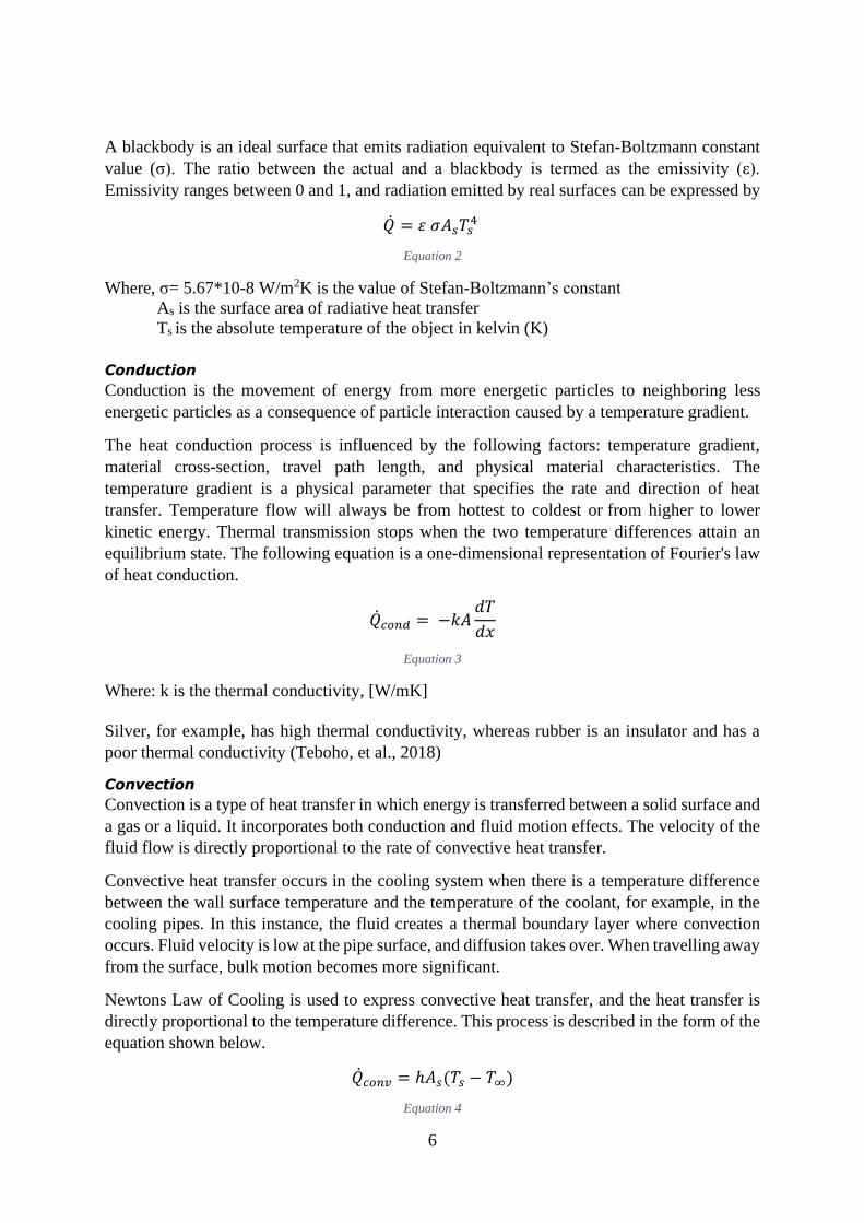
A blackbody is an ideal surface that emits radiation equivalent to Stefan-Boltzmann constant

value (σ). The ratio between the actual and a blackbody is termed as the emissivity (ε).

Emissivity ranges between 0 and 1, and radiation emitted by real surfaces can be expressed by

�� = 𝜀 𝜎𝐴𝑠𝑇𝑠4

Equation 2

Where, σ= 5.67*10-8 W/m2K is the value of Stefan-Boltzmann’s constant

As is the surface area of radiative heat transfer

Ts is the absolute temperature of the object in kelvin (K)

Conduction

Conduction is the movement of energy from more energetic particles to neighboring less

energetic particles as a consequence of particle interaction caused by a temperature gradient.

The heat conduction process is influenced by the following factors: temperature gradient,

material cross-section, travel path length, and physical material characteristics. The

temperature gradient is a physical parameter that specifies the rate and direction of heat

transfer. Temperature flow will always be from hottest to coldest or from higher to lower

kinetic energy. Thermal transmission stops when the two temperature differences attain an

equilibrium state. The following equation is a one-dimensional representation of Fourier's law

of heat conduction.

��𝑐𝑜𝑛𝑑 = −𝑘𝐴𝑑𝑇

𝑑𝑥

Equation 3

Where: k is the thermal conductivity, [W/mK]

Silver, for example, has high thermal conductivity, whereas rubber is an insulator and has a

poor thermal conductivity (Teboho, et al., 2018)

Convection

Convection is a type of heat transfer in which energy is transferred between a solid surface and

a gas or a liquid. It incorporates both conduction and fluid motion effects. The velocity of the

fluid flow is directly proportional to the rate of convective heat transfer.

Convective heat transfer occurs in the cooling system when there is a temperature difference

between the wall surface temperature and the temperature of the coolant, for example, in the

cooling pipes. In this instance, the fluid creates a thermal boundary layer where convection

occurs. Fluid velocity is low at the pipe surface, and diffusion takes over. When travelling away

from the surface, bulk motion becomes more significant.

Newtons Law of Cooling is used to express convective heat transfer, and the heat transfer is

directly proportional to the temperature difference. This process is described in the form of the

equation shown below.

��𝑐𝑜𝑛𝑣 = ℎ𝐴𝑠(𝑇𝑠 − 𝑇∞)

Equation 4

7

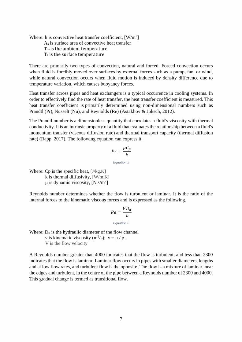
Where: h is convective heat transfer coefficient, [W/m2]

As is surface area of convective heat transfer

T∞ is the ambient temperature Ts is the surface temperature

There are primarily two types of convection, natural and forced. Forced convection occurs

when fluid is forcibly moved over surfaces by external forces such as a pump, fan, or wind,

while natural convection occurs when fluid motion is induced by density difference due to

temperature variation, which causes buoyancy forces.

Heat transfer across pipes and heat exchangers is a typical occurrence in cooling systems. In

order to effectively find the rate of heat transfer, the heat transfer coefficient is measured. This

heat transfer coefficient is primarily determined using non-dimensional numbers such as

Prandtl (Pr), Nusselt (Nu), and Reynolds (Re) (Astakhov & Joksch, 2012).

The Prandtl number is a dimensionless quantity that correlates a fluid's viscosity with thermal

conductivity. It is an intrinsic property of a fluid that evaluates the relationship between a fluid's

momentum transfer (viscous diffusion rate) and thermal transport capacity (thermal diffusion

rate) (Rapp, 2017). The following equation can express it.

𝑃𝑟 =𝜇𝐶𝑝

𝑘

Equation 5

Where: Cp is the specific heat, [J/kg.K]

k is thermal diffusivity, [W/m.K]

μ is dynamic viscosity, [N.s/m2]

Reynolds number determines whether the flow is turbulent or laminar. It is the ratio of the

internal forces to the kinematic viscous forces and is expressed as the following.

𝑅𝑒 =𝑉𝐷ℎ

𝑣

Equation 6

Where: Dh is the hydraulic diameter of the flow channel

ν is kinematic viscosity (m2/s); ν = μ / ρ.

V is the flow velocity

A Reynolds number greater than 4000 indicates that the flow is turbulent, and less than 2300

indicates that the flow is laminar. Laminar flow occurs in pipes with smaller diameters, lengths

and at low flow rates, and turbulent flow is the opposite. The flow is a mixture of laminar, near

the edges and turbulent, in the centre of the pipe between a Reynolds number of 2300 and 4000.

This gradual change is termed as transitional flow.

8

2.2.2 Types of Cooling Systems Engine cooling systems are classified into two categories, air cooling systems and liquid

cooling systems. Air cooling systems were only used in older vehicles and except for some

modern motorcycles. Instead, nowadays, the liquid cooling system plays an essential role in

the automotive industry (Lin & Sundén, 2010).

Air-Cooling Systems

Air cooling systems are commonly used in motorcycle engines and aircraft engines. In these

systems, the heat created by the combustion in the engine cylinders is dissipated by air.

This type of cooling systems has a few advantages in comparison to the liquid cooling system

(Prudhvi, et al., 2013):

• The system is lighter since it does not have a radiator and pump.

• There are no leakages in the air-cooling system.

• It can be used at cold temperatures without the need for antifreeze.

However, the air-cooling systems have some disadvantages (Prudhvi, et al., 2013):

• It is less efficient than a liquid cooling system.

• The engine needs to be exposed directly to the air, as in motorcycles and aircraft.

Liquid Cooling Systems

In the liquid cooling systems, the coolant is usually a mixture of water and ethylene glycol.

The coolant absorbs the heat from the engine and is cooled in the radiator. After this, the coolant

is recirculated to the engine.

Sometimes, oil is also used in liquid cooling systems, especially in the engine and electric

motor. Oil, apart from cooling, also serves the following functions (Palmgren & Hjälm

Wallborg, 2015):

• It lubricates and protects components from corrosion.

• It cleans surfaces and transports pollution particles to the oil filter.

There are two types of liquid cooling system (Lin & Sundén, 2010):

Thermo Siphon System

The circulation of liquid in this system is done by a change in density produced by the

difference in temperatures. As a result, no pump is needed, and the coolant is circulated solely

due to density differences.

Pump Circulation System

In this type, a pump is used to circulate the coolant as was described in Convection in section

2.2.1.

The advantages of liquid cooling systems are (Prudhvi, et al., 2013):

• It dissipates the heat from the engine in a uniform way.

• The engine fuel consumption is improved by using this system.

• Using a liquid cooling system provides more freedom regarding the position of the

engine inside the vehicle.

9

• The liquid absorbs the noise; as a consequence, the engine is less noisy than air-cooled

engines.

On the other hand, the liquid cooling systems also have some disadvantages (Prudhvi, et al.,

2013):

• The quantity of coolant inside the system affects the efficiency of the cooling system.

• The pump consumes a considerable amount of power.

• If the system fails, the engine may suffer severe damage.

• The complexity and the cost of the liquid cooling system are more significant than in

the air-cooling system. Additionally, it requires further maintenance and care for the

components.

In this thesis, the circuit studied is based on a liquid cooling pump circulation system.

2.3 Main Components of a Cooling System

In this section, the main components of a cooling system are explained.

Pipes and Hoses

Pipes and hoses are used to link the various parts of a coolant system together and transport the

coolant mixture between these components. Hence, they should be designed in such a manner

as to be able to endure elevated pressures and temperatures which may exist in the coolant

system.

Hoses must be durable enough at lower ambient temperatures and should also endure sudden

vibrations in the cooling circuit. Furthermore, the pipes and hoses within the circuit should

have an appropriate radius not to allow unwanted pressure losses.

Expansion Tank

Usually, the expansion tank is positioned at the top of the cooling system containing air and

coolant.

The Expansion Tank or Accumulator serves several functions:

• It can be used to fill the coolant in the circuit.

• It provides an additional amount of coolant, which appears when the coolant

temperature rises and helps to retain a specific pressure in the system. If the pressure

exceeds the desired level, a pressure valve opens, letting out some air.

• It also acts as a deaeration device by providing a small flow to direct the air pockets out

of the system, thereby reducing the air in the circuit. This significantly improves the

cooling efficiency of the system.

Pump

The pump is used to drive the coolant through the cooling system. When the coolant passes

through multiple components in the system, the velocity changes due to the pressure losses.

The pump overcomes these pressure losses caused by different components. The electric pumps

are used in the BEV cooling system to maintain an adequately pressurised flow of coolant at

every operational speed. An advantage of using an electric pump is that the coolant flow can

10

be stopped entirely when not needed and offers a higher control precision., unlike mechanical,

where the pump speed depends on the engine speed.

Pump Cavitation

A phenomenon called cavitation occurs when air traps are formed on the suction side of the

pump, causing damage to the pump and rotor blades. Air pockets are mainly caused due

to insufficient Net Positive Suction Head (NPSH). or inadequate priming. Cavitation can

severely reduce the life of a pump, and the collapsing vapour bubbles inside the pump causes

the following problems (Xylem Applied Water Systems, 2015):

• It decreases the pumping capacity.

• Due to the decreased pumping capacity, the pump may not keep up with the incoming

flow, causing overflows.

• It causes excessive vibrations that may damage the rotating elements. For example, the

impeller collides with non-rotating elements, like the wear ring or plates, and can cause

bearing and seals to break before their expected end of life.

• Cavitation can also cause wetted components to be damaged due to contact with

imploding vapour bubbles. The energy generated when the vapour bubbles collapse

causes bits of metal to break off and collide with other moving parts.

Radiator

To dissipate heat efficiently, two radiators, one each for HT and LT circuits, are used. The

radiator for the HT circuit is larger due to higher temperatures within the circuit. A radiator is

a plate heat exchanger that uses metal plates to transfer heat between two fluids. This type of

heat exchanger offers a substantial advantage over the traditional heat exchanger in that the

fluids are subjected to a much greater surface area, so the fluids are dispersed across the plates.

This promotes heat transfer and significantly increases the rate of temperature change (Kakaç,

et al., 2002).

Radiator Fan

A fan is a critical part of the cooling system as it allows air to move through the core of the

radiator constantly. The air is driven into the radiator due to ram air when the vehicle is moving

at high speeds, and the fan supplies additional air flow, causing heat from the engine to

dissipate, cooling the fluid and, as a result, the battery, power electronics and the electric motor.

Electric fans used in the BEV trucks work with a sensor and engage according to the

temperature of the circuit, independent of the drive shaft.

2.4 ICE Trucks

The ICE trucks are powered by a heat engine in which fuel, usually gasoline or diesel, is used

for combustion. During combustion, the engine produces a lot of heat, and a cooling system is

needed. These systems typically feature a radiator, a radiator fan, a coolant pump, and a

thermostat valve, as shown in Figure 2.2, that dissipates the engine's waste heat through the

coolant fluid. The valve is a balancing device that ensures that the engine coolant temperature

stays within the specified range. The coolant fluid is typically a mixture of water and ethylene-

glycol that stays below its boiling point over the engine's entire operating range, including its

maximum heat load (Chastain, 2006).

11

Figure 2.2 ICE Cooling System (Based on ( (Lajunen, et al., 2018))

2.5 BEV Trucks

BEV trucks utilise electric motors and batteries instead of combustion and fuel to produce

power required to drive the vehicle. The battery is the most critical and complex part of an EV

(X-Engineer, 2021). Therefore, significant R&D costs are incurred during the development

of technical solutions which are capable of maintaining the optimum temperature of the

batteries.

Since the battery's working temperatures are different from the rest of the components, the

cooling system is generally formed by two different loops: the LT loop, including the battery

and the HT, including the electric motor, inverter, and power electronics in Figure 2.3.

12

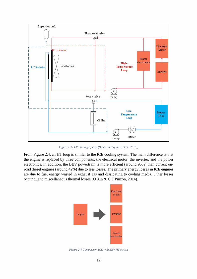
Figure 2.3 BEV Cooling System (Based on (Lajunen, et al., 2018))

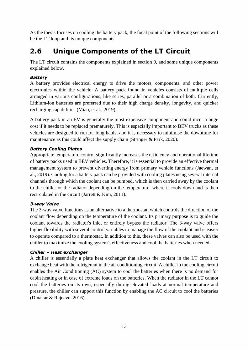
From Figure 2.4, an HT loop is similar to the ICE cooling system. The main difference is that

the engine is replaced by three components: the electrical motor, the inverter, and the power

electronics. In addition, the BEV powertrain is more efficient (around 95%) than current on-

road diesel engines (around 42%) due to less losses. The primary energy losses in ICE engines

are due to fuel energy wasted in exhaust gas and dissipating to cooling media. Other losses

occur due to miscellaneous thermal losses (Q.Xin & C.F.Pinzon, 2014).

Figure 2.4 Comparison ICE with BEV HT circuit

13

As the thesis focuses on cooling the battery pack, the focal point of the following sections will

be the LT loop and its unique components.

2.6 Unique Components of the LT Circuit

The LT circuit contains the components explained in section 0, and some unique components

explained below.

Battery

A battery provides electrical energy to drive the motors, components, and other power

electronics within the vehicle. A battery pack found in vehicles consists of multiple cells

arranged in various configurations, like series, parallel or a combination of both. Currently,

Lithium-ion batteries are preferred due to their high charge density, longevity, and quicker

recharging capabilities (Miao, et al., 2019).

A battery pack in an EV is generally the most expensive component and could incur a huge

cost if it needs to be replaced prematurely. This is especially important to BEV trucks as these

vehicles are designed to run for long hauls, and it is necessary to minimise the downtime for

maintenance as this could affect the supply chain (Stringer & Park, 2020).

Battery Cooling Plates

Appropriate temperature control significantly increases the efficiency and operational lifetime

of battery packs used in BEV vehicles. Therefore, it is essential to provide an effective thermal

management system to prevent diverting energy from primary vehicle functions (Jaewan, et

al., 2019). Cooling for a battery pack can be provided with cooling plates using several internal

channels through which the coolant can be pumped, which is then carried away by the coolant

to the chiller or the radiator depending on the temperature, where it cools down and is then

recirculated in the circuit (Jarrett & Kim, 2011).

3-way Valve

The 3-way valve functions as an alternative to a thermostat, which controls the direction of the

coolant flow depending on the temperature of the coolant. Its primary purpose is to guide the

coolant towards the radiator's inlet or entirely bypass the radiator. The 3-way valve offers

higher flexibility with several control variables to manage the flow of the coolant and is easier

to operate compared to a thermostat. In addition to this, these valves can also be used with the

chiller to maximize the cooling system's effectiveness and cool the batteries when needed.

Chiller – Heat exchanger

A chiller is essentially a plate heat exchanger that allows the coolant in the LT circuit to

exchange heat with the refrigerant in the air conditioning circuit. A chiller in the cooling circuit

enables the Air Conditioning (AC) system to cool the batteries when there is no demand for

cabin heating or in case of extreme loads on the batteries. When the radiator in the LT cannot

cool the batteries on its own, especially during elevated loads at normal temperature and

pressure, the chiller can support this function by enabling the AC circuit to cool the batteries

(Dinakar & Rajeeve, 2016).

14

Heater

In lower or sub-zero temperatures, it is important to heat the coolant to warm the battery.

Modern high voltage heaters that can simultaneously achieve cabin and battery heating are

designed for Direct Current (DC) input voltages between 250 V and 500 V or even up to 800

V to facilitate faster battery charging (BorgWarner, 2020).

2.6.1 Battery Thermal Issues

As a battery is crucial for BEV trucks, it is particularly important to maintain the condition of

the battery, including its temperature. Temperature uniformity is also essential to maintain the

balance between cells in series strings. Temperature variations in the pack cause nonuniform

cell breakdown, affecting cell balance and lowering pack efficiency. The optimum range to get

the best performance of the battery is between 15 °C and 35 °C (Lajunen, et al., 2018).

Otherwise, permanent damage will be caused to the batteries.

The current carrying capacity during discharging reduces as the operating temperature

decreases (Li & Zhu, 2014). The reduced discharge capacity reduces the energy supplied by

the battery (Hu, et al., 2020). Furthermore, the cell resistance rises, limiting the battery's power

output (Hu, et al., 2020). Charging the battery at high voltages and low temperatures is likely

to cause lithium plating, which often results in substantial battery capacity fade (Li & Zhu,

2014). Lithium plating is the deposition of metallic lithium on the surface of the anode of

lithium-ion batteries (Zimmerman & Quinzio, 2010). Therefore, the battery is typically charged

at low voltages at low temperatures to prevent lithium plating, thereby significantly increasing

charge durations (Hu, et al., 2020).

If the battery reaches temperatures above 50 °C, its lifetime and charging efficiency are reduced

(Sato, 2001). Additionally, at high temperatures, the heat dissipation increases, causing thermal

runaway. In thermal runaway, the temperature keeps rising unless heat is dissipated faster than

generated when it reaches a temperature around 80 °C (Gao, et al., 2019). Thermal runaway

comprises many steps, each of which causes more significant damage to the battery cells. At

80 °C, the Solid Electrolyte Interphase (SEI) surface dissolves into the electrolyte. After the

SEI layer is decomposed, the electrolyte starts to react with the anode. This is an exothermal

reaction, which raises the temperature. In the second step, the elevated temperature (around

110 °C) allows organic solvents to degrade, resulting in the emission of hydrocarbon gases.

The gas increases pressure within the cells, and the temperature rises above the flashpoint.

However, because of the lack of oxygen, the gas does not ignite. Then, at 135°C, the separator

melts and short-circuits between the anode and cathode. Finally, the metal-oxide cathode

degrades at 200 ºC and releases oxygen, causing the electrolyte and hydrocarbon gases to ignite

(Feng, et al., 2018).

2.7 Air Traps

During filling, the air is displaced by the coolant towards the highest point in the circuit, i.e.

towards the expansion tank and eventually exiting to the atmosphere. The coolant passes

through many components in a circuit on its way to the expansion tank, resulting in locations

where airlocks can potentially be formed. On a component level, a higher number of cooling

channels may lead to higher chances of the formation of air traps. Air traps, also known as

15

airlocks, are large air bubbles formed by the accumulated air in the circuit that cannot be

released into the atmosphere (OARDS Automotive Hub, 2020). As the air density is less than

the coolant, the air traps are commonly formed in the highest points of the system (Evans

Cooling Systems Australasia, 2016).

The complexity of the LT loop can produce air traps inside the cooling circuit. Each of the

components is placed at different points in 3D space and are connected by hoses. This means

that there could be elevation differences between components and changes in geometries that

may lead to air traps. The low levels of coolant in that section can create an air trap acting as

an insulator for heat convection and decrease the cooling circuit's efficiency, especially near

the components that need to be cooled or heated (Evans Cooling Systems Australasia, 2016)

which can restrict the coolant flow in that section of a pipe.

2.7.1 Two-phase fluid flow

The interactive flow of two distinct phases, say air and water, with common interfaces in, for

example, a pipe is referred to as two-phase flow. The fact that two-phase flows can take several

different shapes and forms is one of the most difficult aspects of dealing with it. It is important

to consider the spatial distribution and velocities of the two phases in the flow channel in many

engineering fields. In order to classify flow pattern, two fundamental parameters of flow should

be understood, which are (White, 2010):

1. Flow Quality – When two-phase fluid flow is considered, a dimensionless fraction

called flow quality is used to represent the air flow inside the total flow. The following

equation defines the flow quality.

𝑥 =��𝑎

��𝑣+��𝑎=

𝑣𝑎𝐴𝑎𝜌𝑎

𝑣𝑎𝐴𝑎𝜌𝑎+ 𝑣𝑙𝐴𝑙𝜌𝑙

Equation 7

In this equation, the subscripts "a" and "v" represent the air and liquid phase,

respectively.

2. Flow rate – Volumetric flow rate, "Q" can be defined as the volume of the fluid, "V"

that flows through a cross-sectional area, "A" per unit time. The following equation

makes it easier to understand.

𝑄 =𝑉

𝑡= 𝐴

𝑑

𝑡

Equation 8

16

Where: 𝑑

𝑡 is the length of the volume of the fluid divided by the time taken for the fluid to

flow through its length.

Therefore,

𝑄 = 𝐴𝑣

Equation 9

Where: v is the velocity of the fluid

Both the flow quality and the flow rate are dependent on the type of fluid and pressure.

This section briefly explains and categorises the simultaneous flow of liquid water and gas

flowing through a duct or a pipe according to the flow direction relative to the gravitational

acceleration, i.e., vertical, or horizontal tubes. An illustration of the flow pattern in vertical

tubes is shown in Figure 2.5.

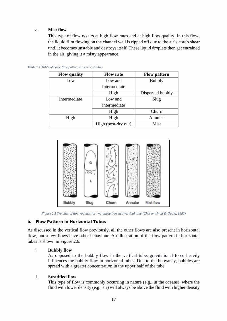
a. Flow Pattern in Vertical Tubes

i. Bubbly flow

In this type of flow, the liquid flow rate is high and causes air to break into bubbles,

but the rate is not high enough for the bubbles to get evenly dispersed throughout

the liquid phase. This flow results in bubbles concentrated at the top half of the tube

due to the buoyancy effect.

ii. Slug flow

At higher air velocities, bubbles tend to agglomerate and slugs similar to the

dimension of the tube are observed. Since these big gas slugs are split from one

another by liquid slugs, they induce significant pressure and liquid flow rate

variations. However, in some cases, even if the net movement of fluid is upward, a

downward flow can be seen near the tube wall, which can be attributed to the effects

of gravitational force.

iii. Churn flow

Churn flow, also known as froth flow, is a particularly distorted two-phase fluid

flow. When the velocity of a slug flow increases, the flow structure becomes

unstable. The appearance of a very thick and turbulent liquid layer, with the liquid,

often alternating up and down, characterizes churn flow. It is one of the least

understood gas-liquid flow regimes due to its almost unstable properties.

iv. Annular flow

Annular flow is observed at higher air velocities in which the liquid forms a

continuous film around the wall of the tube, and the gas flows in a continuous phase

in the centre of the tube. In this type of flow, the flow core can contain dispersed

liquid droplets.

17

v. Mist flow

This type of flow occurs at high flow rates and at high flow quality. In this flow,

the liquid film flowing on the channel wall is ripped off due to the air’s core's shear

until it becomes unstable and destroys itself. These liquid droplets then get entrained

in the air, giving it a misty appearance.

Table 2.1 Table of basic flow patterns in vertical tubes

Figure 2.5 Sketches of flow regimes for two-phase flow in a vertical tube (Cheremisinoff & Gupta, 1983)

b. Flow Pattern in Horizontal Tubes

As discussed in the vertical flow previously, all the other flows are also present in horizontal

flow, but a few flows have other behaviour. An illustration of the flow pattern in horizontal

tubes is shown in Figure 2.6.

i. Bubbly flow As opposed to the bubbly flow in the vertical tube, gravitational force heavily

influences the bubbly flow in horizontal tubes. Due to the buoyancy, bubbles are

spread with a greater concentration in the upper half of the tube.

ii. Stratified flow

This type of flow is commonly occurring in nature (e.g., in the oceans), where the

fluid with lower density (e.g., air) will always be above the fluid with higher density

Flow quality Flow rate Flow pattern

Low Low and

Intermediate

Bubbly

High Dispersed bubbly

Intermediate Low and

intermediate

Slug

High Churn

High High Annular

High (post-dry out) Mist

18

(e.g., liquid water). If the air's velocity increases, the horizontal interface becomes

more disrupted, and waves can form. This flow regime is commonly referred to as

stratified-wavy flow.

iii. Plug or Slug flow1

When the velocity of the air is increased further, the flow could either be

characterized as plug flow, if the diameter of the bubbles is smaller than the tube or

slug flow, if the diameter of the bubbles formed is similar to that of the tube

Table 2.2 Table of basic flow patterns in horizontal tubes.

Figure 2.6 Sketches of flow regimes for two-phase flow in a horizontal pipe (Cheremisinoff & Gupta, 1983)

1 Plug flow model solver of GT-Suite is not the same as the plug flow of the two-phase fluid flow. In GT-Suite a

plug flow solver means that all the subvolumes are calculated sequentially for each element of the circuit.

Flow quality Flow rate Flow pattern

Low Low and

Intermediate

Bubbly

Low Stratified

Intermediate Stratified Wavy

Intermediate Low and

intermediate

Plug and Slug

High High Annular

High (post-dry out) Mist

19

2.8 Computational Fluid Dynamics (CFD)

Computational Fluid Dynamics is the method of calculating and simulating processes

involving heat transfer, fluid flow, and associated phenomena to solve a given problem using

various computational schemes and data structures. CFD equations are calculated by

discretising the domain into smaller sections called elements, which are then solved using

various numerical schemes. In general, this approach is used to produce results similar to those

provided by Computer-Aided Engineering (CAE) in structural mechanics. CFD is based on the

Navier-Stokes equations, which describes the behaviour of the majority of the single-phase

flows to solve the flow problems.

2.8.1 1D vs 3D CFD Simulations

a. 1D CFD Simulation

1D simulations attempt to improve system efficiency by assisting engineers in understanding

the interactions of the system's numerous components. There are a few steps involved in

developing a model for a system (Zhang, 2020):

1. Enter the required components and connect them.

2. Assign the appropriate physical models to the various components (for example,

simplified turbomachines/heat exchangers, pipes, flow resistance, pressure drops, etc.).

3. Enter the necessary physical model parameters

4. Run the simulation

Each component is simulated independently, with its own set of input and values. This

means that the model accurately depicts the system's performance since it considers the

interactions of the various components with one another.

b. 3D CFD Simulations

3D simulations depict the interaction of individual components with their environment,

whereas 1D simulations depict the overall design of a system and the interactions of its

components. As a result, a 1D simulation is ideal for improving the design of a complete

system, whereas a 3D simulation is ideal for finding the optimal design features of specific

components such as flow pattern around a blade or heat transfer with internal cooling air and

exterior hot gas. A 3D simulation may also be used to confirm the results of a 1D simulation,

such as pump cavitation prediction on an NPSH map (Zhang, 2020).

To cater to the requirements of this thesis, a software called GT-Suite, developed by Gamma

Technologies, was used for 1D CFD simulation. It is a commonly used tool among most major

vehicle manufacturers. This section explains the fluid flow in pipes through an internal network

calculated by GT-Suite.

2.8.2 Equations Governing GT-Suite

In GT-Suite, the solutions for the conservation equations of continuity, energy, and

momentum, also known as the Navier-Stokes equations, are calculated in one dimension (1D),

yielding results that are averaged around the direction of flow (Gamma Technologies, 2020).

These equations are:

20

Conservation of Continuity:

𝑑𝑚

𝑑𝑡= ∑ ��

𝑏𝑜𝑢𝑛𝑑𝑎𝑟𝑖𝑒𝑠

Equation 10

Conservation of Energy (Explicit Solver in GT-Suite):

𝑑(𝑚𝑒)

𝑑𝑡= −𝜌

𝑑𝑉

𝑑𝑡+ ∑ (��𝐻) − ℎ𝐴𝑠(𝑇𝑓𝑙𝑢𝑖𝑑 − 𝑇𝑤𝑎𝑙𝑙)


Equation 11

Conservation of Enthalpy (Implicit Solver in GT-Suite):

𝑑(𝑝𝐻𝑉)

𝑑𝑡= 𝑉

𝑑𝑉

𝑑𝑡+ ∑ (��𝐻) − ℎ𝐴𝑠(𝑇𝑓𝑙𝑢𝑖𝑑 − 𝑇𝑤𝑎𝑙𝑙)


Equation 12

Conservation of Momentum:

𝑑��

𝑑𝑡=

𝑑𝑝𝐴 + ∑ (𝑚𝐻) − 4𝐶𝑓𝑝𝑢|𝑢|

2

𝑑𝑥𝐴𝐷 − 𝐾𝑝(

12 𝑝𝑢|𝑢|)𝐴𝑏𝑜𝑢𝑛𝑑𝑎𝑟𝑖𝑒𝑠

𝑑𝑥

Equation 13

where:

m: Boundary mass flux into volume, m = ρAu

m: Mass of volume

V: Volume

p: Pressure

ρ: Density

A: Cross-sectional flow area

As: Heat transfer surface area

e: Internal energy + Kinetic energy per unit mass

H: Total specific enthalpy, H = e + p

ρ

h: Heat transfer coefficient

Tfluid: Fluid temperature

Twall: Wall temperature

u: Velocity at the boundary

Cf: Fanning friction factor

Kp: Pressure loss coefficient

D: Equivalent diameter

dx: Length of mass element in flow direction (discretization length)

dp: Pressure differential acting across dx

Time integration approaches are divided into two types (Gamma Technologies, 2020):

21

• Explicit: This type of integration is preferred when the wave dynamics are crucial, such

as engine air flows, acoustics and fuel injection systems. This method is not desirable

for simulations that run for longer than a minute as it focuses on accurate predictions

of pressure pulsations.

• Implicit: This type of integration is used in cooling systems, air conditioning and

lubrication when the Mach number is less than 0.3, and the wave dynamics are not an

essential parameter of consideration. This method is ideal for simulations that run in

the order of minutes.

2.8.3 Discretisation in GT-Suite

To accurately model the system, the system is discretised into several volumes called

computational cells where each flow split is represented by one volume and every pipe is

divided into single or more volumes. This type of discretization is known as a "staggered grid"

and a schematic shown in Figure 2.7. In this approach, the scalar variables like pressure,

temperature, density, enthalpy, internal energy are approximated to be uniform over each

volume. The vector variables such as rate of mass flow, velocity, etc., are calculated for each

cell boundary. The larger discretisation results in less accurate results, but the computational

time is significantly faster. Smaller discretisation results in higher accuracy but requires a much

longer computational time which increases exponentially as the discretisation is made finer.

Figure 2.7 Discretisation in GT-Suite

2.8.4 Pressure Drops

The difference in pressure between two points in a fluid-carrying network is referred to as

pressure drop. When frictional forces induced by the flow resistance act on a fluid as it passes

through the tube, a pressure drop occurs. The key determinants of fluid flow resistance are fluid

velocity through the pipe and fluid viscosity (Gamma Technologies, 2020).

Generally, pressure losses in pipes occur due to irregular cross-sections, bends, and tapers,

which can be accounted for by setting the pressure loss coefficient. GT-Suite handles the

pressure drops by adjusting three distinct parameters (Gamma Technologies, 2020):

22

Pressure Loss Coefficient

The pressure loss coefficient (Kp) is defined as:

𝐾𝑝 =𝑝1 − 𝑝2

12 𝜌𝑉1

2

Equation 14

Where: p2 is total pressure at inlet,

p1: Total pressure at outlet,

ρ: Inlet density and

V1=Inlet Velocity

By using the default option for pressure loss coefficient, an internal calculation of losses within

the cones and bends is performed by the software. This does not include the effects of wall

friction, which is calculated separately, as explained in the next section.

Friction losses

Flow losses within pipes caused by friction along the walls are automatically determined as a

function of Reynolds number and wall surface roughness using a Fanning friction factor.

The Moody Diagram, which represents the relationship between Reynolds number, wall

roughness, and the resulting friction factor, is mathematically determined by the implicit

Colebrook equation; however, for better solution speed, an explicit approximation of the

Colebrook equation is used (Cruz, et al., 2012). GT-Suite offers three options to have trade-

offs between speed and accuracy: simple, improved, and a third one that applies both the

improved friction and the bend loss model. The automatic choice selects one of the three for

all nodes and automatically selects the most appropriate method (Gamma Technologies, 2020).

Heat Transfer

A heat transfer coefficient quantifies heat transfer from fluids between the pipes and at the flow

split to their walls. A heat transfer coefficient is determined at each timestep using the velocity

of the fluid, thermophysical properties like thermal conductivity, viscosity, specific heat,

density, and wall surface roughness. In GT-Suite, the heat transfer coefficient of smooth pipes

can be calculated using the Colburn analogy, Dittus-Boelter, Gnielinski, or Sieder-Tate, with

the Colburn analogy being the default option. This correlation is represented by the following

equation (Gamma Technologies, 2020).

ℎ𝑔 = (1

2)𝐶𝑓𝜌𝑈𝑒𝑓𝑓𝐶𝑝𝑃𝑟(−

23

)

Equation 15

23

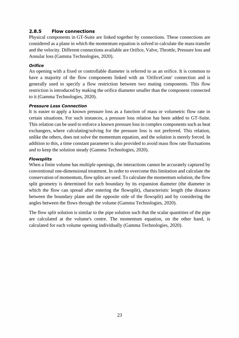
2.8.5 Flow connections

Physical components in GT-Suite are linked together by connections. These connections are

considered as a plane in which the momentum equation is solved to calculate the mass transfer

and the velocity. Different connections available are Orifice, Valve, Throttle, Pressure loss and

Annular loss (Gamma Technologies, 2020).

Orifice

An opening with a fixed or controllable diameter is referred to as an orifice. It is common to

have a majority of the flow components linked with an 'OrificeConn' connection and is

generally used to specify a flow restriction between two mating components. This flow

restriction is introduced by making the orifice diameter smaller than the component connected

to it (Gamma Technologies, 2020).

Pressure Loss Connection

It is easier to apply a known pressure loss as a function of mass or volumetric flow rate in

certain situations. For such instances, a pressure loss relation has been added to GT-Suite.

This relation can be used to enforce a known pressure loss in complex components such as heat

exchangers, where calculating/solving for the pressure loss is not preferred. This relation,

unlike the others, does not solve the momentum equation, and the solution is merely forced. In

addition to this, a time constant parameter is also provided to avoid mass flow rate fluctuations

and to keep the solution steady (Gamma Technologies, 2020).

Flowsplits

When a finite volume has multiple openings, the interactions cannot be accurately captured by

conventional one-dimensional treatment. In order to overcome this limitation and calculate the

conservation of momentum, flow splits are used. To calculate the momentum solution, the flow

split geometry is determined for each boundary by its expansion diameter (the diameter in

which the flow can spread after entering the flowsplit), characteristic length (the distance

between the boundary plane and the opposite side of the flowsplit) and by considering the

angles between the flows through the volume (Gamma Technologies, 2020).

The flow split solution is similar to the pipe solution such that the scalar quantities of the pipe

are calculated at the volume's centre. The momentum equation, on the other hand, is

calculated for each volume opening individually (Gamma Technologies, 2020).

24

3 Methodology This chapter presents the selected research strategy and data collection method used to answer

the research question. It also subsequently discusses the steps involved in the data interpretation

process and explains how different cases were set up to validate the experiments performed

Two different test rigs were built and studied in this project - auxiliary and Scania’s test rig.

The objective for the auxiliary test rig was to understand modelling and simulation using

CATIA V5 and GT-Suite. The Scania test rig was built to perform more realistic tests, as the

components used on it can be found in a truck. In both the test rigs, different cases were

designed to study the coolant and the air behaviour.

3.1 Auxiliary Test Rig

3.1.1 Case Definitions

The Auxiliary test rig was divided into two cases, Horizontal and Vertical. As shown in Figure

3.1 in blue, the Horizontal case was formed by two pipes placed horizontal (Volume 1 and

Volume 2). The main objective was to study the flow pattern in horizontal tubes, explained in

section b, during a filling. In the Vertical case, in red in Figure 3.1, Volume 2 was replaced

with a hose creating a loop before the expansion device. By creating the loop, some parts of

the hose are vertical allowing the authors to observe the flow pattern in vertical tubes, as

explained in section a.. All the hoses in the circuit were transparent in order to see how the

circuit was filled and detect any air trap.

Figure 3.1 Auxiliary Test Rig Scheme

25

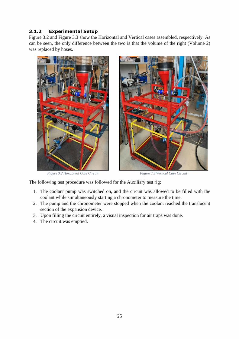
3.1.2 Experimental Setup

Figure 3.2 and Figure 3.3 show the Horizontal and Vertical cases assembled, respectively. As

can be seen, the only difference between the two is that the volume of the right (Volume 2)

was replaced by hoses.

Figure 3.2 Horizontal Case Circuit

Figure 3.3 Vertical Case Circuit

The following test procedure was followed for the Auxiliary test rig:

1. The coolant pump was switched on, and the circuit was allowed to be filled with the

coolant while simultaneously starting a chronometer to measure the time.

2. The pump and the chronometer were stopped when the coolant reached the translucent

section of the expansion device.

3. Upon filling the circuit entirely, a visual inspection for air traps was done.

4. The circuit was emptied.

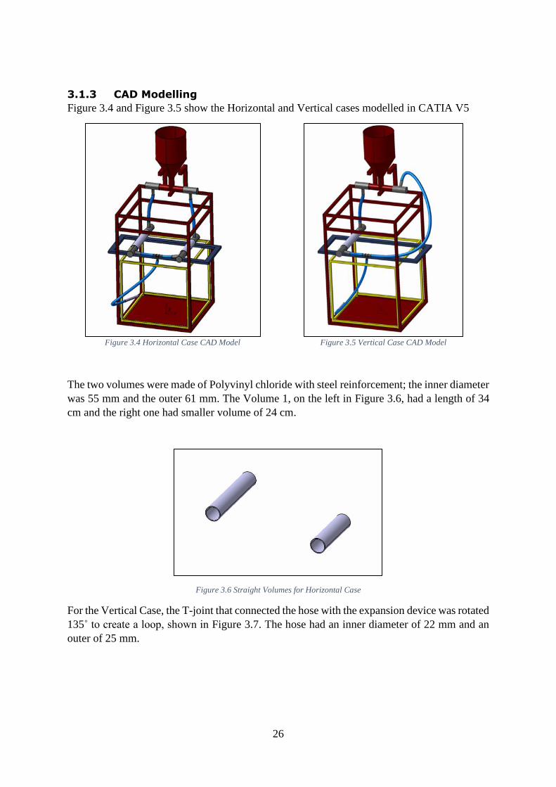
26

3.1.3 CAD Modelling

Figure 3.4 and Figure 3.5 show the Horizontal and Vertical cases modelled in CATIA V5

Figure 3.4 Horizontal Case CAD Model

Figure 3.5 Vertical Case CAD Model

The two volumes were made of Polyvinyl chloride with steel reinforcement; the inner diameter

was 55 mm and the outer 61 mm. The Volume 1, on the left in Figure 3.6, had a length of 34

cm and the right one had smaller volume of 24 cm.

Figure 3.6 Straight Volumes for Horizontal Case

For the Vertical Case, the T-joint that connected the hose with the expansion device was rotated

135˚ to create a loop, shown in Figure 3.7. The hose had an inner diameter of 22 mm and an

outer of 25 mm.

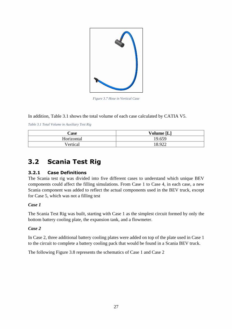
27

Figure 3.7 Hose in Vertical Case

In addition, Table 3.1 shows the total volume of each case calculated by CATIA V5.

Table 3.1 Total Volume in Auxiliary Test Rig

Case Volume [L]

Horizontal 19.659

Vertical 18.922

3.2 Scania Test Rig

3.2.1 Case Definitions

The Scania test rig was divided into five different cases to understand which unique BEV

components could affect the filling simulations. From Case 1 to Case 4, in each case, a new

Scania component was added to reflect the actual components used in the BEV truck, except

for Case 5, which was not a filling test

Case 1

The Scania Test Rig was built, starting with Case 1 as the simplest circuit formed by only the

bottom battery cooling plate, the expansion tank, and a flowmeter.

Case 2

In Case 2, three additional battery cooling plates were added on top of the plate used in Case 1

to the circuit to complete a battery cooling pack that would be found in a Scania BEV truck.

The following Figure 3.8 represents the schematics of Case 1 and Case 2

28

Figure 3.8 Cases 1 and 2 Scheme

Case 3

Case 3 was distinguished from Case 2 with an addition of a mixing line. The mixing line (also

referred to as a distribution line) is a component designed by Scania, which simultaneously

works as a junction from which the coolant is distributed to various components and a

deaeration device. The mixing line has a unique shape that facilitates the air trapped in the

circuit to reach the expansion tank through the static line, after which the air escapes o the

atmosphere. Thus, this device reduces the probability of air being recirculated in the cooling

circuit and battery cooling.

Case 4

Case 4 was formed by adding a pump to Case 3. This water pump recirculates the coolant in

the cooling circuit and the battery cooling plates, ensuring that the batteries work at the

optimum temperature during the truck’s operation.

The following Figure 3.9 represents the schematics of Case 3 and Case 4

29

Figure 3.9 Cases 3 and 4 Scheme

Case 5

Figure 3.10 represents Case 5, and the circuit layout was the same as Case 4. However, the

coolant pump which filled the coolant in the circuit was switched OFF, and the inlet valve was

closed. This was done to examine how the operation of the pump released the air by monitoring

the fluid level in the expansion tank.

30

Figure 3.10 Case 5 Scheme

3.2.2 Experimental Setup

The experimental procedure was the same as the auxiliary test rig but with the addition of a

flowmeter. A flowmeter was added to the circuit to read the coolant's flowrate and use it as an

input to GT-Suite. The ideal position to install the flowmeter would have been after the coolant

pump; however, this could not be done due to limitations in space and was placed after the

right cooling rod instead.

In every case, the test was run three times at three different flow rates to observe how the flow

affects the filling and the creation of air traps in the circuit. Since a rotational valve regulated

the coolant pump, it was challenging to have repeatability in flow rates between the test runs.

Table 3.2 presents the flowrate readings for every case and test run.

The battery cooling plates were not emptied every time due to difficulties in manually turning

over the plates each time after filling. However, to measure the volume of the coolant, the

cooling plates were emptied after Case 2, Test Run 1 and Case 4, Test Run 1. The following

procedure was used to empty the plates:

a. The clamps holding the battery cooling plates together with the cooling rods were loosened.

b. The battery cooling plates were then disconnected from the cooling rod and turned upside-

down, which allowed the coolant to drain from the inlet and the outlet ports into a beaker.

c. This process was carried out sequentially, starting from the top to the bottom cooling plate.

Despite best efforts, some amount of coolant was spilt every time this process was carried out

and could not be measured, which could lead to a significant source of error.

31

Case 1

1. The coolant pump was switched on, and the circuit was allowed to be filled with the

coolant while simultaneously starting a chronometer to measure the time.

2. The pump and the chronometer were stopped when the coolant reached the translucent

section of the expansion device.

3. Upon filling the circuit entirely, a visual inspection for air traps was done.

Case 2

The procedure was the same as in Case 1, and the volume of the coolant in the cooling plates

was measured after Test Run 1

Case 3

The procedure was the same as in Case 1

Case 4

The procedure was the same as in Case 1, and the volume of the coolant in the cooling plates

was measured after Test Run 1

Table 3.2 Flowrate readings

Case Test Run Flowrate [L/min]

1

1 18.9

2 15.4

3 8.1

2

1 15.0

2 12.7

3 12.6

3

1 15.7

2 12.5

3 10.4

4

1 16.3

2 12.3

3 7.1

Since the plates were not emptied in Case 2 (Test Run 2 and Test Run 3), an assumption was

made to accommodate this arrangement. Seven additional seconds were added to the total time

measured by the chronometer. This was assumed because seven seconds was the average time

to fill the cooling plates in Case 2.

Furthermore, another significant difference from the auxiliary test rig was the location of the

cooling inlet. In the auxiliary test rig, the coolant inlet was placed in the lowest point of the

circuit while, in the Scania test rig, it was located 106.098mm above the bottom-most cooling

plate, as shown in Figure 3.11.

32

Figure 3.11 Cooling Inlet

Case 5

As mentioned before, Case 5 was not a filling. Therefore, the test procedure for this case was:

1. After filling in case 4, the cooling inlet was unplugged, and the valve was closed.

2. The pump was turned on while simultaneously starting a chronometer to measure the

time.

3. Every 20 seconds, the volume of the coolant in the expansion tank was measured and

noted. It was determined that if there was air trapped in the circuit, then the coolant

volume in the expansion tank would drop as the air traps were removed. This behaviour

was observed for 6 minutes, after which the test was concluded.

This test was run twice, one with the pump at full speed (25 L/min) and the other at half speed

(13.3 L/min).

3.2.3 CAD Modelling

In the Scania test rig, all cases included the battery cooling plates, the expansion tank and the

flowmeter. These components were common to all the cases.

Only one cooling plate was modelled, shown in Figure 3.12 below, and was further duplicated.

The total capacity of one cooling plate was 0.503 L.

Figure 3.12 Cooling plate CAD Model (based on Appendix 1)

33

The expansion tank, Figure 3.13, had a total capacity of 11.2 L. Nevertheless, for safety

reasons, the expansion tank had to be filled between the MAX and MIN lines, corresponding

to 5.5 L and 3.8 L, respectively.

Figure 3.13 Expansion Tank CAD Model

The volumes of the main components from the Scania test rig are stated in the Table 3.3 below.

Table 3.3 Main Component Volumes

Component Volume [L]

Cooling Plate 0.503

Expansion Tank 5.500

Left Cooling Rod 0.553

Right Cooling Rod 0.515

Flowmeter 0.080

Mixing Line 2.049

Pump 0.031

Table 3.4 shows the total volume of each case. Case 5 is not included since it had the same

volume as Case 4. The differences in volumes in every case was due to the addition of a new

component.

Table 3.4 Total Volume in Scania Test Rig

Case Volume [L]

1 8.653

2 10.426

3 12.399

4 12.444

All the CAD models for each case are in Appendix 2.

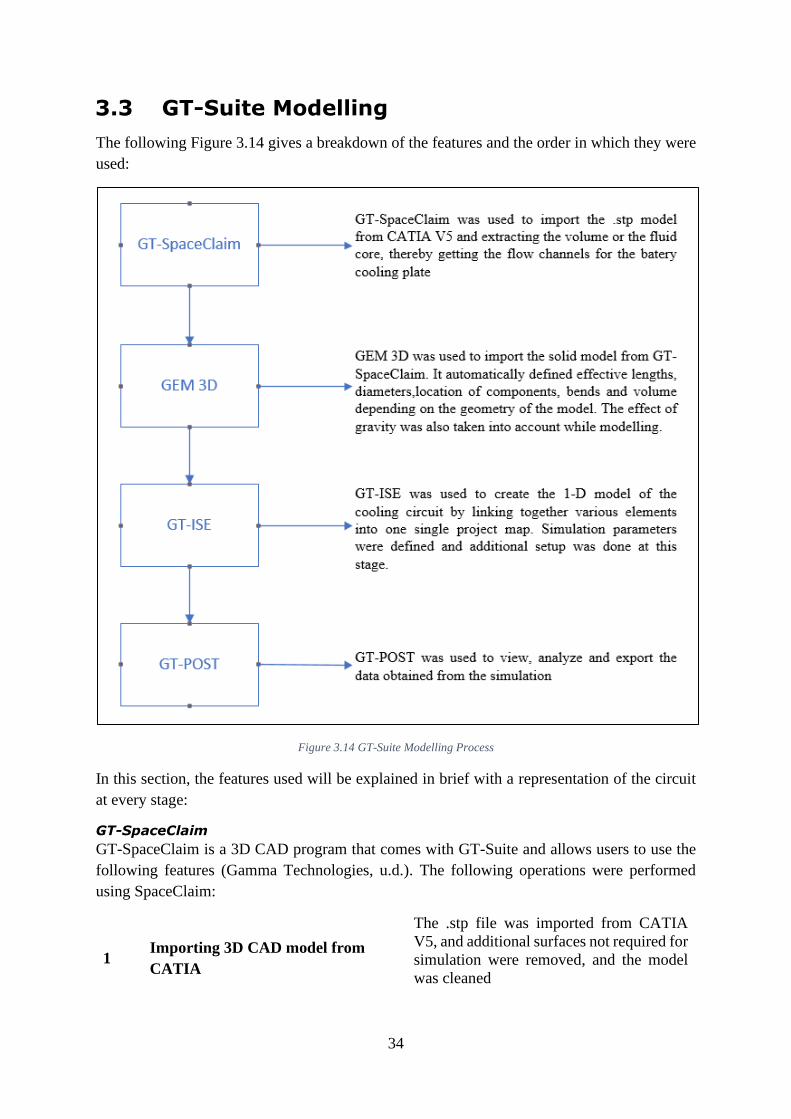
34

3.3 GT-Suite Modelling

The following Figure 3.14 gives a breakdown of the features and the order in which they were

used:

Figure 3.14 GT-Suite Modelling Process

In this section, the features used will be explained in brief with a representation of the circuit

at every stage:

GT-SpaceClaim

GT-SpaceClaim is a 3D CAD program that comes with GT-Suite and allows users to use the

following features (Gamma Technologies, u.d.). The following operations were performed

using SpaceClaim:

1 Importing 3D CAD model from

CATIA

The .stp file was imported from CATIA

V5, and additional surfaces not required for

simulation were removed, and the model

was cleaned

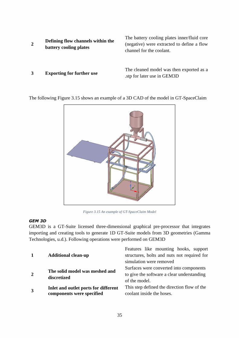
35

2 Defining flow channels within the

battery cooling plates

The battery cooling plates inner/fluid core

(negative) were extracted to define a flow

channel for the coolant.

3 Exporting for further use

The cleaned model was then exported as a

.stp for later use in GEM3D

The following Figure 3.15 shows an example of a 3D CAD of the model in GT-SpaceClaim

Figure 3.15 An example of GT-SpaceClaim Model

GEM 3D

GEM3D is a GT-Suite licensed three-dimensional graphical pre-processor that integrates

importing and creating tools to generate 1D GT-Suite models from 3D geometries (Gamma

Technologies, u.d.). Following operations were performed on GEM3D

1 Additional clean-up

Features like mounting hooks, support

structures, bolts and nuts not required for

simulation were removed

2 The solid model was meshed and

discretized

Surfaces were converted into components

to give the software a clear understanding

of the model.

3 Inlet and outlet ports for different

components were specified

This step defined the direction flow of the

coolant inside the hoses.

36

The 3D model was then converted into a 1D representation by exporting as a .gtsub file with

the following parameters:

1 Pipe Discretization Length

Specifies the length of each sub-element –

30mm was used.

2

Shell Discretization Lengths along

X, Y and Z directions

30mm was used

3

Flowsplit Acceptance ratio

Specifies the percentage of the cube’s

volume that must be present for the flow

split to be retained.- 50% was used

(Rudravajhala, 2018)

The following Figure 3.16 shows the 3D CAD of the model in GEM3D

Figure 3.16 An example of a GEM3D Model

GT-ISE (Integrated Simulation Environment)

GT-ISE is the primary interface for creating models, declaring simulation parameters, and

running simulations. It is an ecosystem in which different elements are brought onto a project

map and linked together to form an overall model (Gamma Technologies, u.d.).

The following steps were performed within GT-ISE:

1 Model and Setup A 1D circuit diagram representing the

coolant flow in the 3D model was set up

with all the components

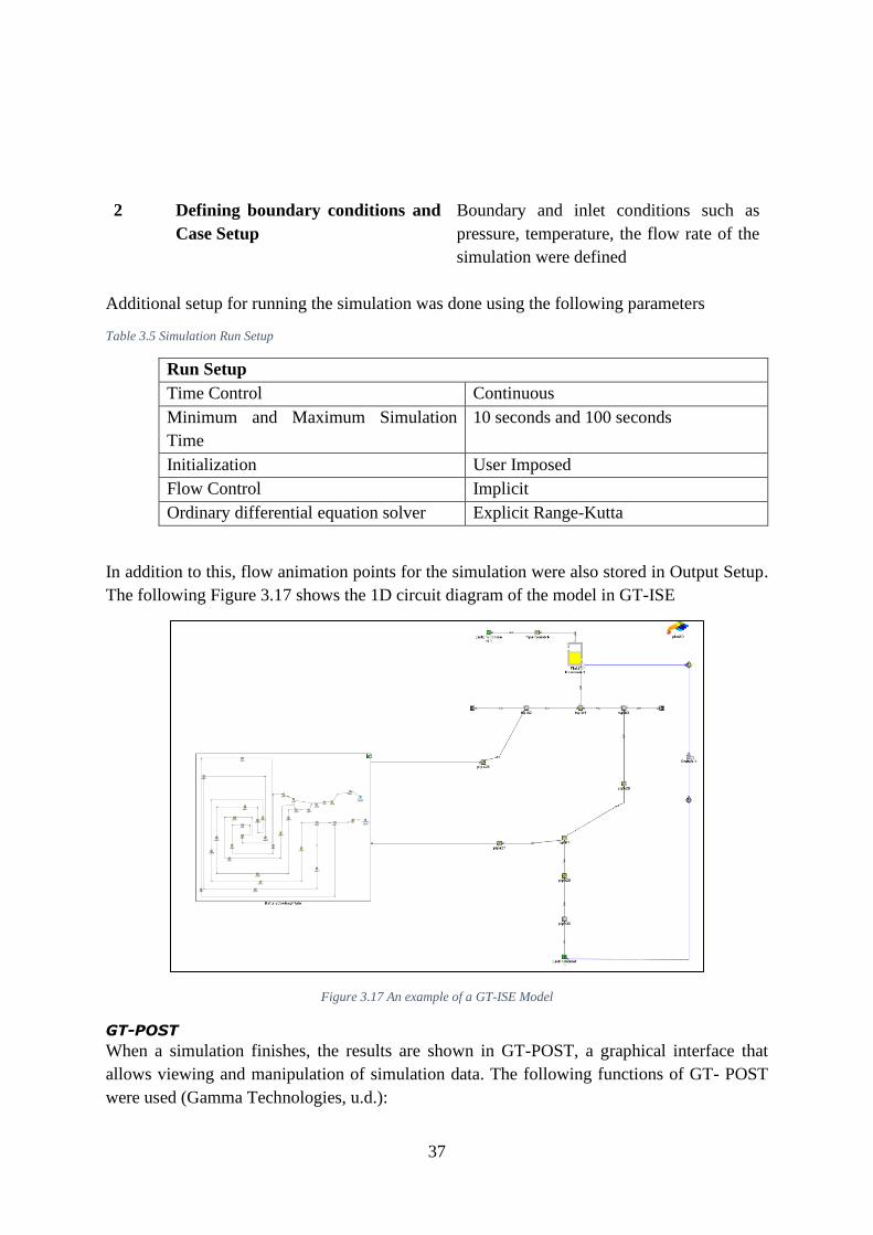
37

2

Defining boundary conditions and

Case Setup

Boundary and inlet conditions such as

pressure, temperature, the flow rate of the

simulation were defined

Additional setup for running the simulation was done using the following parameters

Table 3.5 Simulation Run Setup

Run Setup

Time Control Continuous

Minimum and Maximum Simulation

Time

10 seconds and 100 seconds

Initialization User Imposed

Flow Control Implicit

Ordinary differential equation solver Explicit Range-Kutta

In addition to this, flow animation points for the simulation were also stored in Output Setup.

The following Figure 3.17 shows the 1D circuit diagram of the model in GT-ISE

Figure 3.17 An example of a GT-ISE Model

GT-POST

When a simulation finishes, the results are shown in GT-POST, a graphical interface that

allows viewing and manipulation of simulation data. The following functions of GT- POST

were used (Gamma Technologies, u.d.):

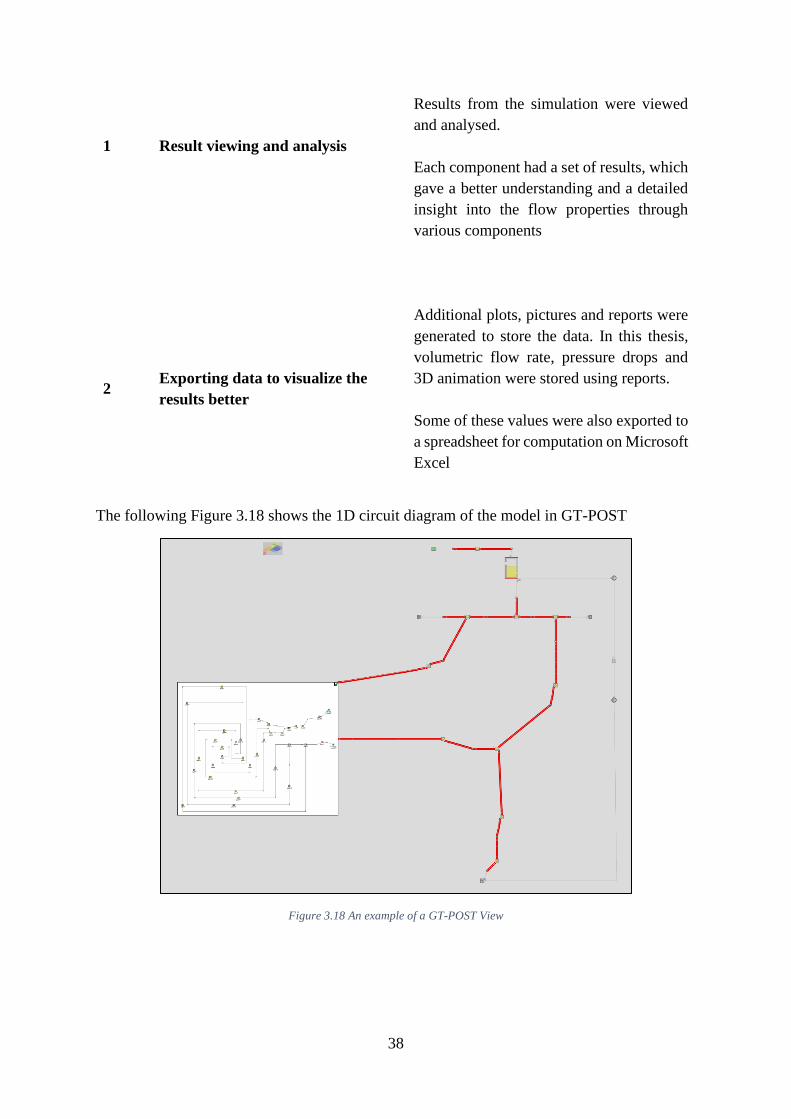
38

1

Result viewing and analysis

Results from the simulation were viewed

and analysed.

Each component had a set of results, which

gave a better understanding and a detailed

insight into the flow properties through

various components

2

Exporting data to visualize the

results better

Additional plots, pictures and reports were

generated to store the data. In this thesis,

volumetric flow rate, pressure drops and

3D animation were stored using reports.

Some of these values were also exported to

a spreadsheet for computation on Microsoft

Excel

The following Figure 3.18 shows the 1D circuit diagram of the model in GT-POST

Figure 3.18 An example of a GT-POST View

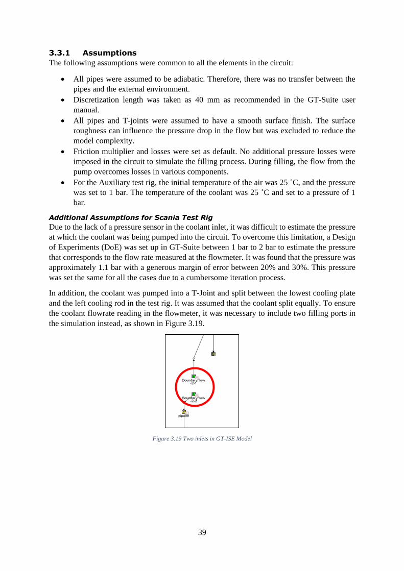
39

3.3.1 Assumptions

The following assumptions were common to all the elements in the circuit:

• All pipes were assumed to be adiabatic. Therefore, there was no transfer between the

pipes and the external environment.

• Discretization length was taken as 40 mm as recommended in the GT-Suite user

manual.

• All pipes and T-joints were assumed to have a smooth surface finish. The surface

roughness can influence the pressure drop in the flow but was excluded to reduce the

model complexity.

• Friction multiplier and losses were set as default. No additional pressure losses were

imposed in the circuit to simulate the filling process. During filling, the flow from the

pump overcomes losses in various components.

• For the Auxiliary test rig, the initial temperature of the air was 25 ˚C, and the pressure

was set to 1 bar. The temperature of the coolant was 25 ˚C and set to a pressure of 1

bar.

Additional Assumptions for Scania Test Rig

Due to the lack of a pressure sensor in the coolant inlet, it was difficult to estimate the pressure

at which the coolant was being pumped into the circuit. To overcome this limitation, a Design

of Experiments (DoE) was set up in GT-Suite between 1 bar to 2 bar to estimate the pressure

that corresponds to the flow rate measured at the flowmeter. It was found that the pressure was

approximately 1.1 bar with a generous margin of error between 20% and 30%. This pressure

was set the same for all the cases due to a cumbersome iteration process.

In addition, the coolant was pumped into a T-Joint and split between the lowest cooling plate

and the left cooling rod in the test rig. It was assumed that the coolant split equally. To ensure

the coolant flowrate reading in the flowmeter, it was necessary to include two filling ports in

the simulation instead, as shown in Figure 3.19.

Figure 3.19 Two inlets in GT-ISE Model

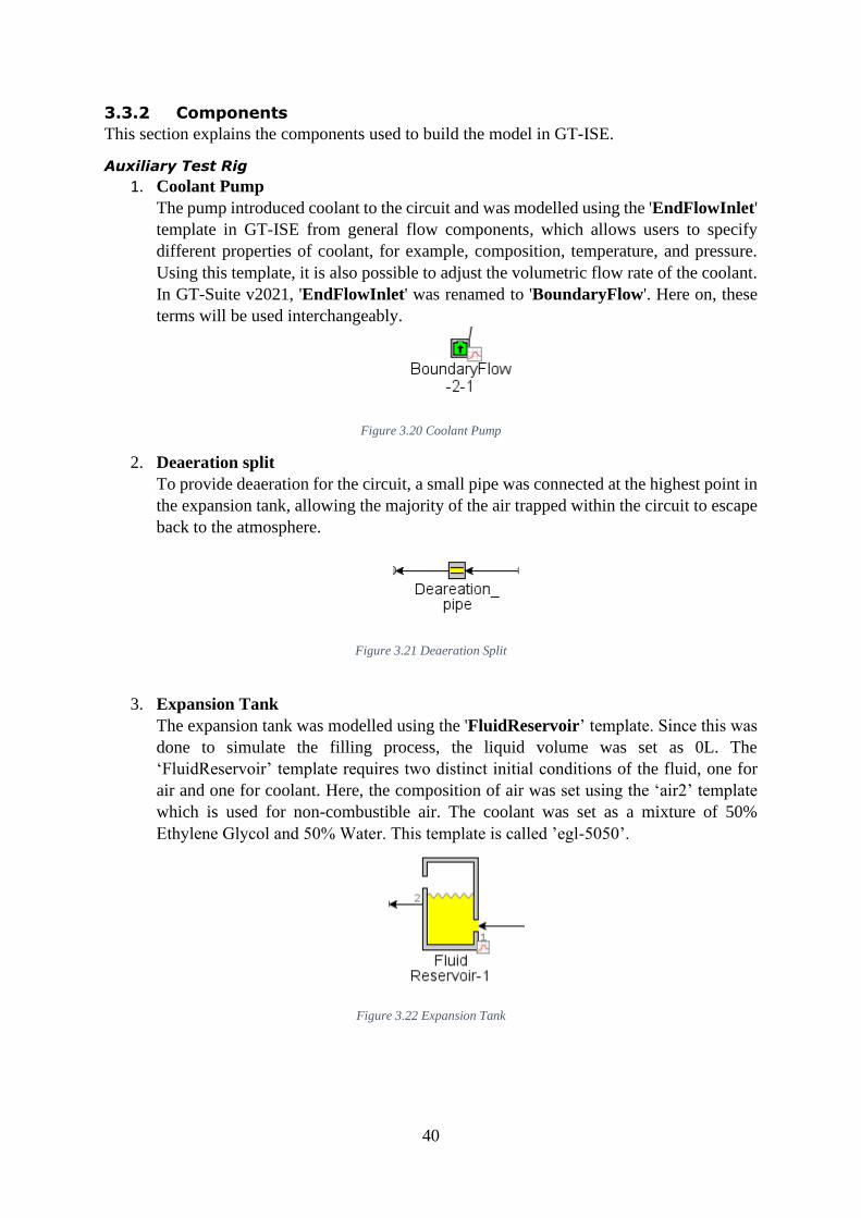
40

3.3.2 Components

This section explains the components used to build the model in GT-ISE.

Auxiliary Test Rig

1. Coolant Pump The pump introduced coolant to the circuit and was modelled using the 'EndFlowInlet'

template in GT-ISE from general flow components, which allows users to specify

different properties of coolant, for example, composition, temperature, and pressure.

Using this template, it is also possible to adjust the volumetric flow rate of the coolant.

In GT-Suite v2021, 'EndFlowInlet' was renamed to 'BoundaryFlow'. Here on, these

terms will be used interchangeably.

Figure 3.20 Coolant Pump

2. Deaeration split

To provide deaeration for the circuit, a small pipe was connected at the highest point in

the expansion tank, allowing the majority of the air trapped within the circuit to escape

back to the atmosphere.

Figure 3.21 Deaeration Split

3. Expansion Tank

The expansion tank was modelled using the 'FluidReservoir’ template. Since this was

done to simulate the filling process, the liquid volume was set as 0L. The

‘FluidReservoir’ template requires two distinct initial conditions of the fluid, one for

air and one for coolant. Here, the composition of air was set using the ‘air2’ template

which is used for non-combustible air. The coolant was set as a mixture of 50%

Ethylene Glycol and 50% Water. This template is called ’egl-5050’.

Figure 3.22 Expansion Tank

41

4. 3-way T-joint

The 3-way T-joints were modelled as flow splits using the template ‘FlowSplitTRight’

in GT ISE from general flow components. This template allows three ports to be

modelled for the T-joint. Port 1 and 2 represent the main line, and port 3 represents the

diameter of the perpendicular.

Figure 3.23 T-Joint

5. End-Flow Caps

To simulate the end of a pipe or a section that was capped off to the flow of the coolant,

a template called ‘EndFlowCap’ was used. In GT-Suite v2021, ‘EndFlowCap’ was

renamed to ‘BoundaryFlowCap’. Here on, these terms will be used interchangeably.

Figure 3.24 End-Flow Claps

6. Coolant and Air

The coolant was modelled using the ‘FluidInitialState’. This template allows the

initialisation of the flow of a fluid with pressure and temperature with humidity and

altitude.

Scania Test Rig

For the Scania test rig, he same components as the auxiliary test rig were modelled. In addition

to these, the flowmeter and the cooling plates were also modelled in GT-ISE.

The flowmeter was modelled using a 'PipeRound' template in GT-ISE from general flow

components. The pipe was modelled as a straight pipe without any bend. The flow meter used

in the test rig indicates the flowrate of the coolant from the pump, but in the case of the

modelling, the flowrate is controlled used the 'EndFlowInlet'.

Figure 3.25 Flowmeter in GT-ISE

42

The volumetric flowrate was measured in the orifices before and after the flowmeter,

highlighted in red in Figure 3.26.

Figure 3.26 Flowrate Measurement in GT-ISE

The cooling plate was modelled as a combination of different ‘PipeRound’ and ‘FlowSplit’,

as shown in Figure 3.27.

Figure 3.27 Battery Cooling Plate in GT-ISE

Case 5

In case 5, initially, during filling, the cooling rods had the flow in the same direction. However,

after the water pump was switched ON, the flow direction in one section reverses after filling.

This allows the coolant to be recirculated within the circuit. In order to account for this, three

new templates were used:

• SensorConn: Senses the volume of the coolant in the expansion tank.

• Switch: The switch receives a signal from the SensorConn and sends the signal to

‘SignalHold.’

• SignalHold: SignalHold retains the min/max value from the switch and sends it to an

‘ActuatorConn.’

• ActuatorConn: This template is used for an actuator for the ‘Switch’ that overrides the

initial input.

43

In this case, when the expansion tank was being filled, volume level signals were sent to the

‘SensorConn’, which passed the signals to the ‘Switch’. The ‘Switch’, depending on whether

the expansion tank was full or not, allowed the flow of coolant from the inlet. When the

expansion tank was full, a signal to stop the filling was sent to ‘EndFlowInlet’ and another to

start the pump.

This circuit setup needs additional fine-tuning to be ready to run and was therefore set as an

optional objective for the thesis work.

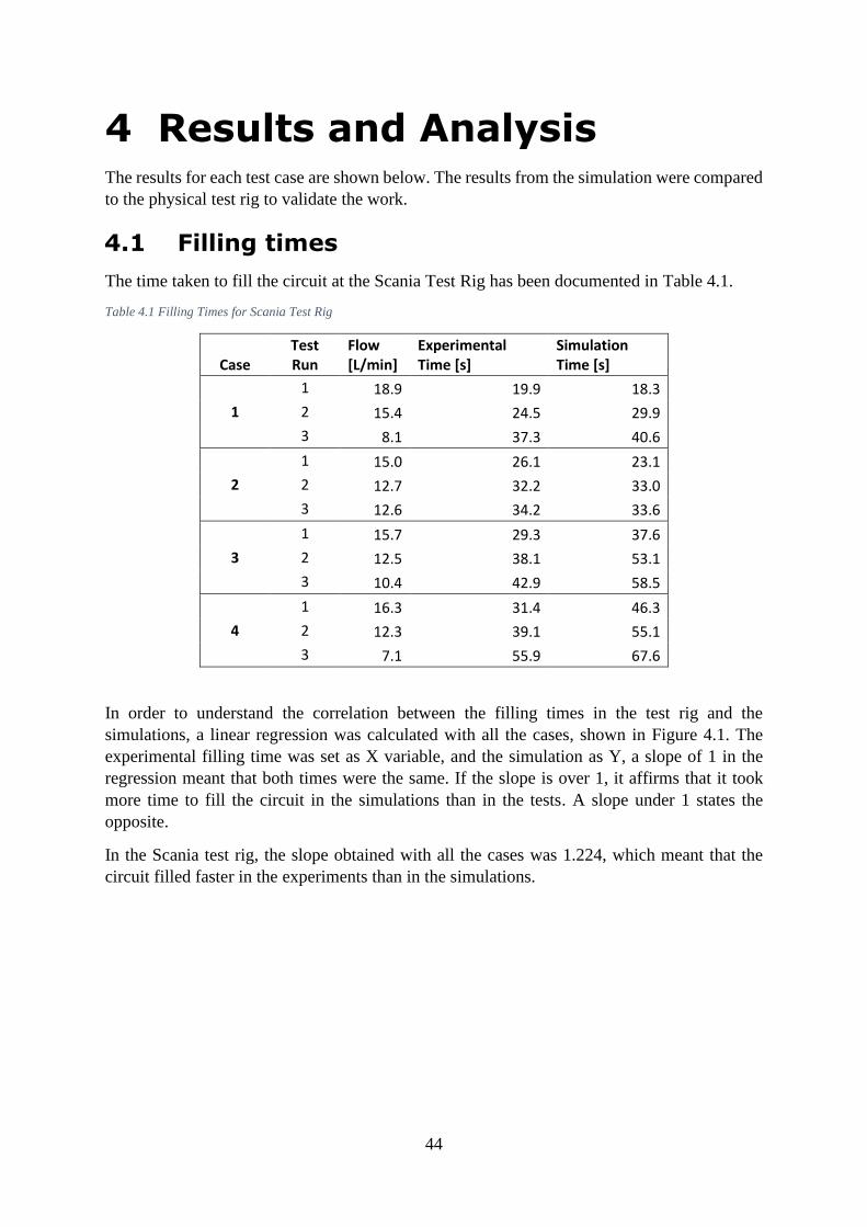
44

4 Results and Analysis The results for each test case are shown below. The results from the simulation were compared

to the physical test rig to validate the work.

4.1 Filling times

The time taken to fill the circuit at the Scania Test Rig has been documented in Table 4.1.

Table 4.1 Filling Times for Scania Test Rig

Case Test Run

Flow [L/min]

Experimental Time [s]

Simulation Time [s]

1

1 18.9 19.9 18.3

2 15.4 24.5 29.9

3 8.1 37.3 40.6

2

1 15.0 26.1 23.1

2 12.7 32.2 33.0

3 12.6 34.2 33.6

3

1 15.7 29.3 37.6

2 12.5 38.1 53.1

3 10.4 42.9 58.5

4

1 16.3 31.4 46.3

2 12.3 39.1 55.1

3 7.1 55.9 67.6

In order to understand the correlation between the filling times in the test rig and the

simulations, a linear regression was calculated with all the cases, shown in Figure 4.1. The

experimental filling time was set as X variable, and the simulation as Y, a slope of 1 in the

regression meant that both times were the same. If the slope is over 1, it affirms that it took

more time to fill the circuit in the simulations than in the tests. A slope under 1 states the

opposite.

In the Scania test rig, the slope obtained with all the cases was 1.224, which meant that the

circuit filled faster in the experiments than in the simulations.

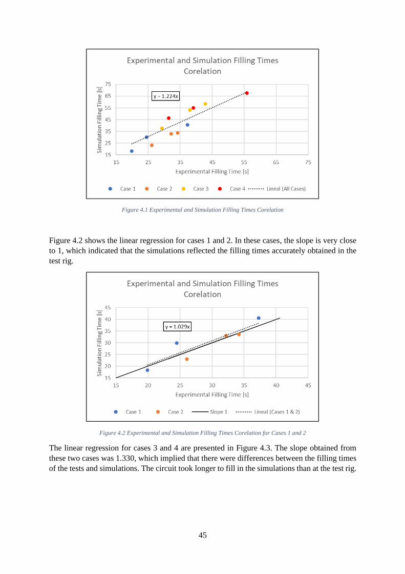
45

Figure 4.1 Experimental and Simulation Filling Times Corelation

Figure 4.2 shows the linear regression for cases 1 and 2. In these cases, the slope is very close

to 1, which indicated that the simulations reflected the filling times accurately obtained in the

test rig.

Figure 4.2 Experimental and Simulation Filling Times Corelation for Cases 1 and 2

The linear regression for cases 3 and 4 are presented in Figure 4.3. The slope obtained from

these two cases was 1.330, which implied that there were differences between the filling times

of the tests and simulations. The circuit took longer to fill in the simulations than at the test rig.

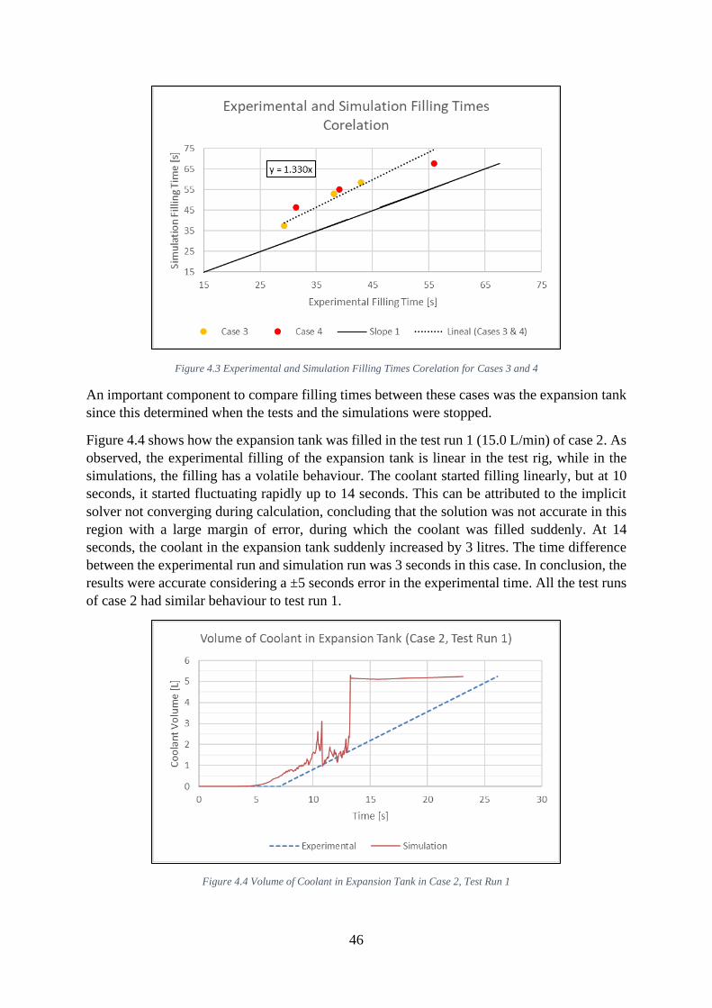
46

Figure 4.3 Experimental and Simulation Filling Times Corelation for Cases 3 and 4

An important component to compare filling times between these cases was the expansion tank

since this determined when the tests and the simulations were stopped.

Figure 4.4 shows how the expansion tank was filled in the test run 1 (15.0 L/min) of case 2. As

observed, the experimental filling of the expansion tank is linear in the test rig, while in the

simulations, the filling has a volatile behaviour. The coolant started filling linearly, but at 10

seconds, it started fluctuating rapidly up to 14 seconds. This can be attributed to the implicit

solver not converging during calculation, concluding that the solution was not accurate in this

region with a large margin of error, during which the coolant was filled suddenly. At 14

seconds, the coolant in the expansion tank suddenly increased by 3 litres. The time difference

between the experimental run and simulation run was 3 seconds in this case. In conclusion, the

results were accurate considering a ±5 seconds error in the experimental time. All the test runs

of case 2 had similar behaviour to test run 1.

Figure 4.4 Volume of Coolant in Expansion Tank in Case 2, Test Run 1

47

In the test run 1 (16.3 L/min) of case 4, plotted in Figure 4.5. The filling of the expansion tank

at the test rig is linear, similar to case 2. In the simulation, the expansion tank started filling

slowly before the test run. At approximately 27 seconds, the coolant stopped filling linearly

and was volatile until 40 seconds. This resulted in the coolant filling the expansion tank

suddenly, as explained in case 2 simulations. After this sudden filling, the expansion tank filled

linearly till the end. Comparing the experimental and simulation filling time, the expansion

tank filled 15 seconds earlier in the experimental run than the simulations.

Figure 4.5 Volume of Coolant in Expansion Tank in Case 4, Test Run 1

4.2 Air traps

4.2.1 Auxiliary Test Rig

Horizontal Case

Figure 4.6 shows the air traps observed in the horizontal case. The type of flow observed was

plug flow in volumes 1 and 2, and the bubbles accumulated at the top of the horizontal hoses.

These air traps always occurred at the same location, despite changing the flow rate and were

attributed to the circuit's geometry. However, as shown in Figure 4.7, GT-Suite failed to

simulate the air traps seen in Figure 4.6.

Upon further investigation, it was found that a 1D approach to flow simulation divides a length

of a pipe into different subvolumes defined by the discretisation length. Inside each subvolume,

the fluid is homogenous, with uniform properties and conditions inside the entire subvolume.

This means that a single subvolume contains a fluid mixture of a uniform quality rather than

tracking the individual bubble movements for a two-phase mixture.

In order to detect an air trap of this scale, a flow model to the pipe solution needs to be added

that tracks the fluid and vapour velocities separately which are not currently available in GT-

Suite.

48

Figure 4.6 Horizontal Case Air Traps

Figure 4.7 Horizontal Case Simulation Results

Vertical Case

The type of flow observed in the volume, in this case, was bubbly at first and completely free

of air when the expansion tank was filled. The only air trap was seen in the loop, which is

highlighted in Figure 4.8. This air trap was primarily due to the geometry of the hose, which

led to the coolant not reaching higher up and filling the circuit. This case was accurately

simulated by GT-Suite as there was only air in this section and not a two-phase mixture of both

coolant and air. The simulated air trap can be seen in Figure 4.9.

Figure 4.8 Vertical Case Air Trap

Figure 4.9 Vertical Case Simulation Results

49

4.2.2 Scania Test Rig

Case 1

In Test Run 1 and Test Run 2, air traps were neither observed in the test rig nor in the

simulations, as shown in Figure 4.10 and Figure 4.11

Figure 4.10 Case 1, Test Run 1 Simulation Results


However, in the third run at 8.1 L/min, a big air trap was seen in the hose that connects the

flowmeter and the T-Joint in the test rig, shown in Figure 4.12.

Figure 4.12 Case 1, Test Run 3 Air Trap

This big air trap was not seen in simulation results, as shown in the hose highlighted in red in

Figure 4.13 at the test rig. GT-Suite flow solver utilizes a sequential flow model through every

pipe and orifice. This means the mass flow moves uniformly across each discretised sub-

volume when the system is balanced, and there is no separation of fluids within a sub-volume.

Whereas, in this test rig, a stratified flow was observed in some cases with coolant and air in

separate layers, which is challenging to capture in a 1D simulation. Predicting this in GT-Suite

poses a challenge because stratification between different fluid densities is not captured.

50


Table 4.2 is derived from section 2.7.1 and summarizes the type of flow observed in case 1 at

the test rig:

Table 4.2 Types of Flow in Case 1

Test Run 1 - 18.9 L/min Bubbly flow at first, no air traps when filled

Test Run 2 - 15.4 L/min Bubbly flow at first, no air traps when filled

Test Run 3 - 8.1 L/min Plug flow in certain sections, some air traps

when filled

Due to the circuit's geometry and the coolant inlet location, it was assumed that the coolant in

the bottom plate was never removed and that it would have the highest amount of coolant. This

assumption showed consistent results and was verified by measuring the plates using the

process mention in 3.2.2 under subsection Case 1.

Case 2

In order to make the circuit more detailed and reflect the test rig, three additional cooling plates

were included in the model and simulated.

During simulating Case 2, it was noticed that GT-Suite does not have a robust model of liquid

flowing along the bottom of a pipe. This was especially pronounced when the three additional

cooling plates were added to the circuit, and the solver had difficulties in converging.

It was observed that the top cooling plate was not entirely filled in Test Run 1, as highlighted

in Figure 4.14. However, this could not be visually validated at the test rig due to the difficulties

mentioned in 3.2.2.

Table 4.3 shows the volume of coolant measured after Test Run 1.

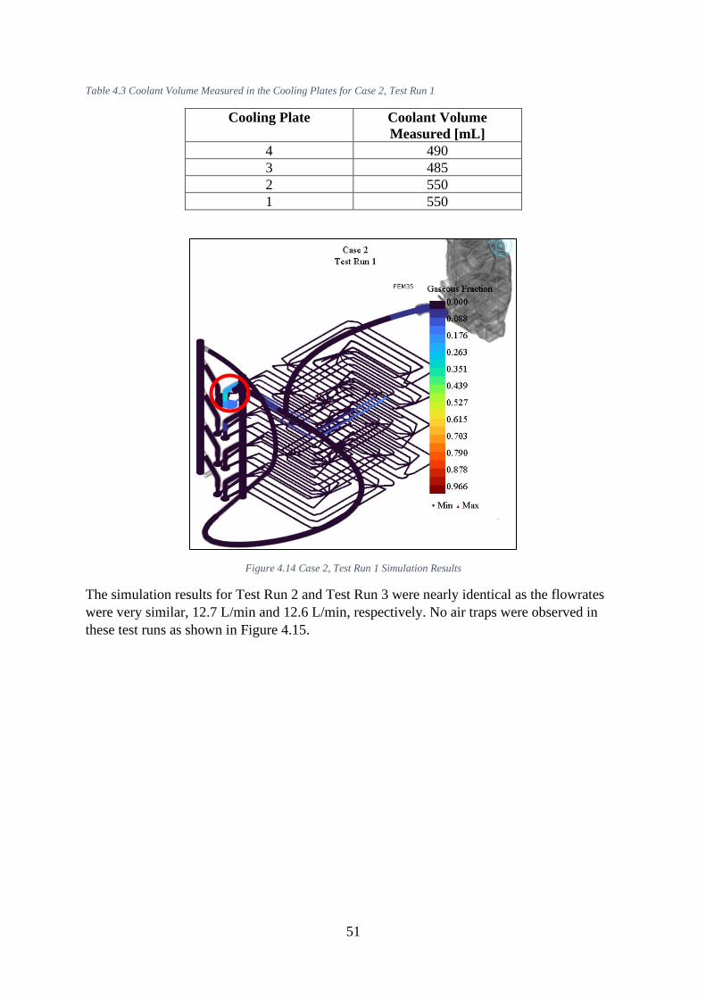
51

Table 4.3 Coolant Volume Measured in the Cooling Plates for Case 2, Test Run 1

Cooling Plate Coolant Volume

Measured [mL]

4 490

3 485

2 550

1 550


The simulation results for Test Run 2 and Test Run 3 were nearly identical as the flowrates

were very similar, 12.7 L/min and 12.6 L/min, respectively. No air traps were observed in

these test runs as shown in Figure 4.15.

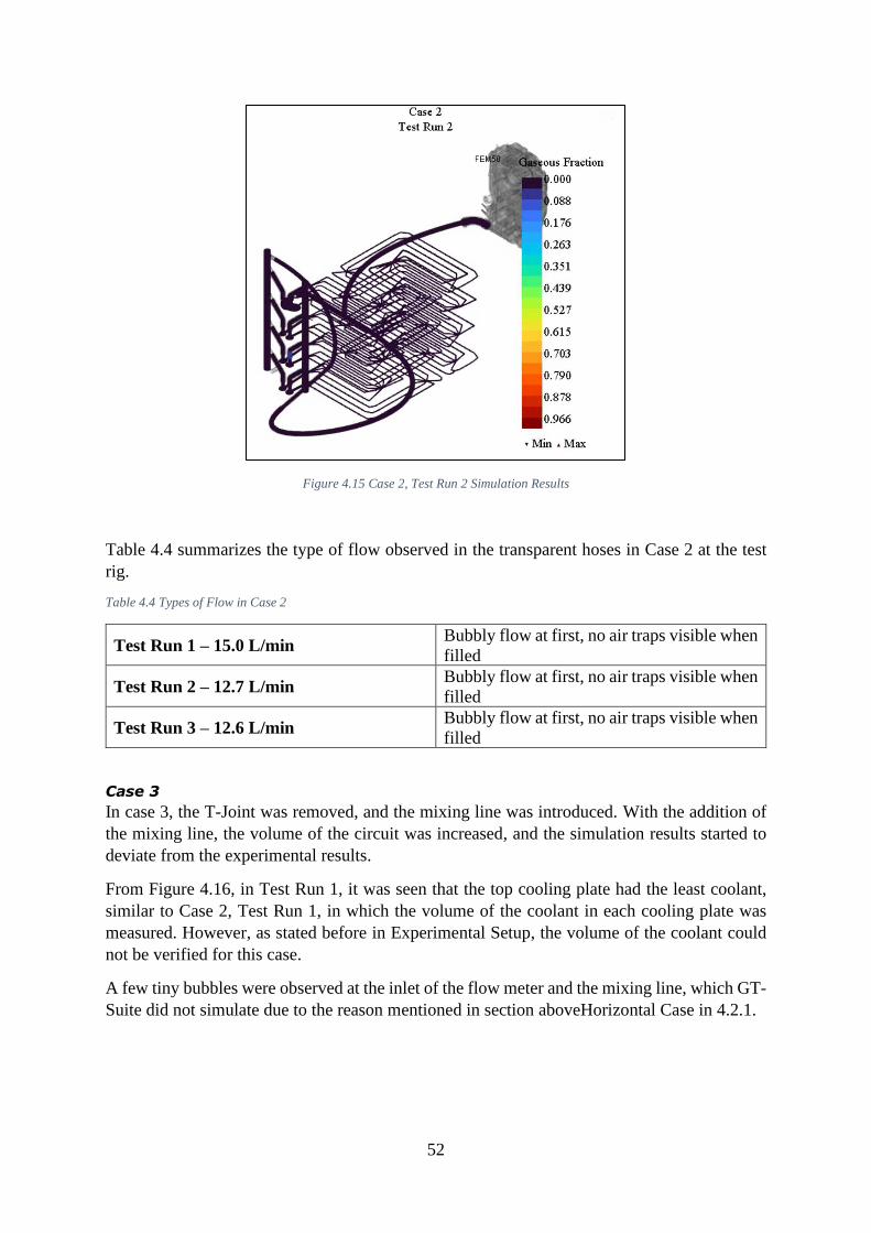
52


Table 4.4 summarizes the type of flow observed in the transparent hoses in Case 2 at the test

rig.


Test Run 1 – 15.0 L/min Bubbly flow at first, no air traps visible when

filled


filled


filled

Case 3

In case 3, the T-Joint was removed, and the mixing line was introduced. With the addition of

the mixing line, the volume of the circuit was increased, and the simulation results started to

deviate from the experimental results.

From Figure 4.16, in Test Run 1, it was seen that the top cooling plate had the least coolant,

similar to Case 2, Test Run 1, in which the volume of the coolant in each cooling plate was

measured. However, as stated before in Experimental Setup, the volume of the coolant could

not be verified for this case.

A few tiny bubbles were observed at the inlet of the flow meter and the mixing line, which GT-

Suite did not simulate due to the reason mentioned in section aboveHorizontal Case in 4.2.1.

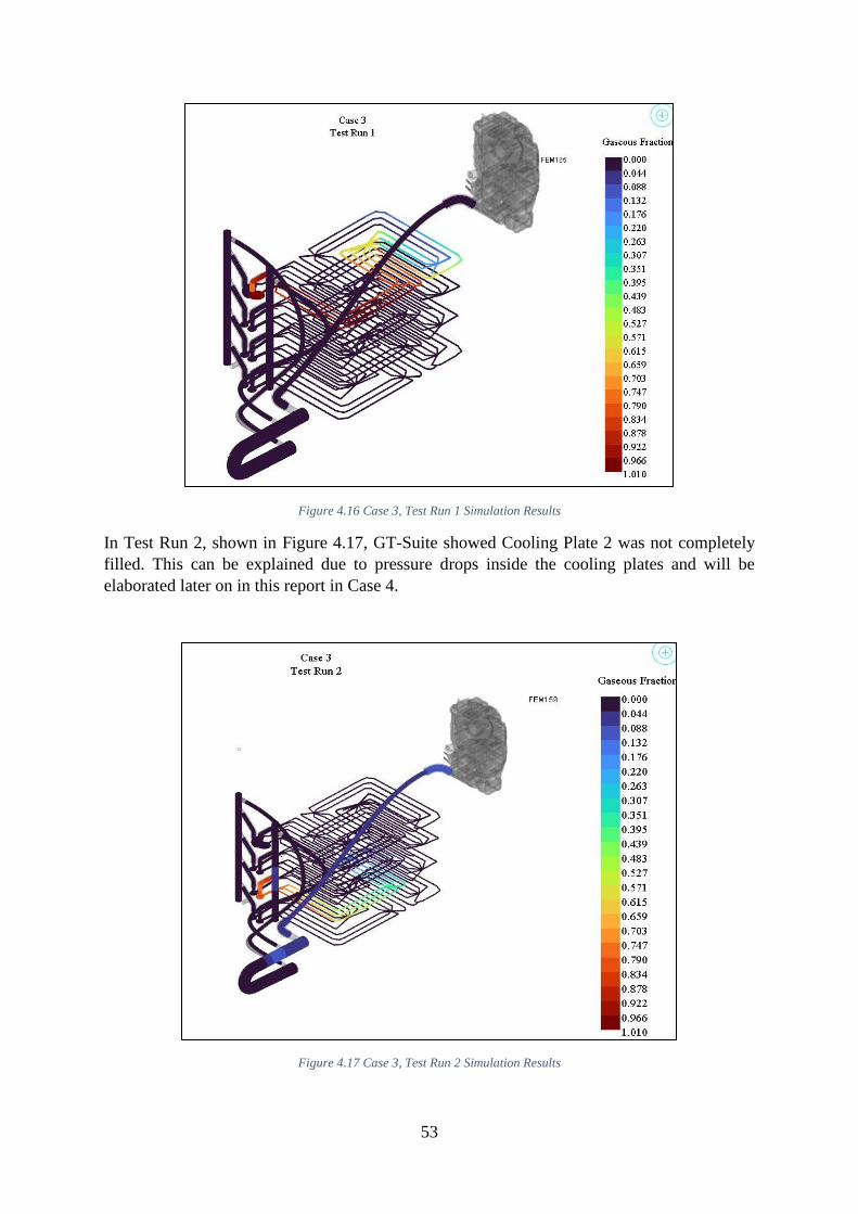
53


In Test Run 2, shown in Figure 4.17, GT-Suite showed Cooling Plate 2 was not completely

filled. This can be explained due to pressure drops inside the cooling plates and will be

elaborated later on in this report in Case 4.


54

In Test Run 3, shown in Figure 4.18, the simulation showed a higher air fraction inside the

mixing line. However, this was not possible to verify as the mixing line was made of steel. In

addition to this, the static line had a minimal amount of air. During filling at the test rig, it was

observed that the trapped bubbles continuously escaped through the mixing line to the

expansion tank.


Table 4.5 summarizes the type flow observed in the transparent hoses in Case 3 at the test rig.


Test Run 1 – 15.7 L/min Bubbly flow at first, no large air traps visible

when filled


when filled


when filled

Case 4

In case 4, the long hose was split into two smaller hoses with a pump in between both the hoses.

This pump was not switched on during the testing, but it added complexity to the circuit's

geometry.

The deviation seen in Case 3 continued in Case 4, with the simulation taking more time to fill

the circuit compared to the experimental test.

Similar to Case 2 and Case 3, the top cooling plate showed air traps in the simulation, shown

in Figure 4.19, and this was verified by emptying the coolant from the cooling plates using the

procedure mentioned in Experimental Setup.

55


In the Test Run 2, shown in Figure 4.20, the Cooling Plate 2 was not entirely filled, similar to

Test Run 2 in Case 3. During the Test Run 2 in both cases, a slight pressure difference was

observed in the simulations between the inlet cooling rod and the inlet to the coolant plates.

Fluid always flows from higher pressure to lower pressure, and the inlet of the cooling plates

always had a higher pressure, causing an airlock, shown in Figure 4.21.


56

Figure 4.21 Case 4, Test Run 2 Pressures

The inlet of the cooling plates was 19 mm, 12 mm less than the inlet of the cooling rod, which

meant that coolant flowed straight up instead of uniformly entering the cooling plates. When

the volumetric flow rate was high, the flow rate instantly dropped, and the coolant failed to

enter the inlet of the plate (Case 3, Test Run 2 and Case 4, Test Run 2). However, this was

incorrect, and it was experimentally found that plate 2 had a significantly higher volume of

coolant, as shown in Table 4.6.

Table 4.6 Coolant Volume Measured in the Cooling Plates for Case 4, Test Run 1

Cooling Plate Coolant Volume

Measured [mL]

4 485

3 473

2 550

1 550

The results from Test Run 3 were very similar to Test Run 3 in Case 3, as shown in Figure

4.22. The air traps were simulated in the mixing line and the top cooling plate, and it was

verified that the top cooling plate (plate 4 in 4.6) had less volume of coolant than in the other

plates. It should be noted that the method employed to measure the volume of the cooling plates

had a big margin of error, as stated in Experimental Setup.

57


Table 4.7 summarizes the type flow observed in the transparent hoses in case 4 at the test rig:



filled


filled

Test Run 3 – 7.1 L/min Plug flow in certain sections, some air traps

visible when filled

Case 5 (running the water pump)

• A circuit for simulating Case 5 was built on GT-ISE to start the water pump at half

speed when the filling stops; however, due to lack of time and software limitations, the

simulation for this case was not completed, only the experimental results were

documented, and a rough model is presented in the section.

For deaeration, an experimental test, Case 5, was built upon the already existing Case 4.

Following results were obtained from Case 5:

• Upon filling till the max line on the expansion tank, it was found that running the pump

reversed the direction of flow and recirculated the coolant to remove the air from the

circuit, which was not removed during filling.

• This led to a drop in the height of the coolant in the expansion tank. When the pump

was run at full speed (approximately 25 L/min), the coolant level had only dropped by

2 mm. At the pump’s half speed (approximately 13 L/min), the coolant had dropped

around 13 mm, as shown in Figure 4.23, which meant that the pump’s operation had

removed approximately 0.41 L trapped air from the circuit.

58

Figure 4.23 Drop in the height of coolant level in the Expansion tank at Case 5 (13 L/min)

• Furthermore, it was observed that larger air traps on passing through the pump were

dispersed as tiny air bubbles throughout the circuit (mist flow from section Flow

Pattern in Horizontal Tubes). This behaviour was predominant when the pump was

run at full speed.

• At the pump’s half-speed, the bubbly flow eventually merged to form a plug flow. This

led to bigger air bubbles being accumulated in the static line and eventually escaping

through the expansion tank during the operation of the pump.

59

5 Discussions

5.1 Filling Times & Air Traps

The expansion tank's port height plays a vital role and has to be carefully selected to avoid

errors during simulations. The air needs someplace to escape to, and this has to be defined

accurately, else the pressure builds up in the circuit, and the simulation fails to execute. It was

observed that GT-Suite gave a fatal error stating that pressure in a specific component is beyond

10,000,000 bar. However, upon discussing this issue with GT support staff, it was found that

port height was responsible for this error and not the component that was displayed in the error

message.

It was concluded that the current version of GT-Suite could not simulate mist flow or bubbly

flow accurately due to the reasons mentioned in section 4.2.1. Since Case 1 and Case 2 showed

similar characteristics and were discussed together. Likewise, Case 3 and Case 4 are also

discussed together due to similar results obtained from both the cases.

5.1.1 Case 1 and 2

• GT-Suite simulated Case 1 and Case 2 circuits better, and the filling time for both the

simulation and the physical test was similar. This was likely because case 1 and case 2

circuits were relatively easier to model in GT-Suite with fewer flowsplits and the

absence of a distribution line. A set of simplifications are made in GT-Suite to calculate

equations that are difficult to solve in 1D, as mentioned in section 2.8.5. As a result,

when the number of flowsplits increases, there is a possibility of reduced accuracy in

the results obtained.

• It was found that low flow rates of the coolant in the circuit attributed to plug flow in

some instances, such as in Case 1 Test Run 3, as summarized in Table 4.2

• In test run 1, case 2, a small air trap was simulated in the top cooling plate, and this was

experimentally verified by measuring the volume of fluid after that test run. At the same

time GT-Suite simulated that the Cooling Plate 3 was completely filled, however this

was incorrect, and it was experimentally proven to have air inside.

5.1.2 Case 3 and 4

• In both Case 3 and Case 4, the simulation results were similar to each other as the

geometry was almost identical, with the exception of a pump in Case 4. However, this

pump did not affect simulations as it was switched off.

• To have higher accuracy in simulations, it is advisable to have the coolant flow in a

single direction. There are higher chances of an airlock when the coolant enters the

cooling plates from both the inlet and outlet directions.

• Upon addition of other components such as the mixing line, three additional cooling

plates, the circuit was more complex in comparison to Case 1 and Case 2. This meant

that additional components that were modelled, which increased the number of

flowsplits and GT Suite struggled to simulate the cases accurately. However, there

could be multiple factors influencing the non-convergence of results and a detailed

study has to be done for different parameter to determine the root cause.

60

• In the simulations, it was observed that pressure drops caused the Cooling Plate 2 not

to be filled; however, after experimentally measuring the volume of the coolant after

the Test Run 1 in Case 4, it was found that GT-Suite simulated this incorrectly, and the

plate was entirely filled by coolant.

5.1.3 Case 5 (Effects of airlocks moving through a water pump)

One method of removing air in the BEV circuit was to run the coolant pump to displace the air

traps. This operation of the coolant pump can be replicated in GT-Suite. In the test rig, it was

observed that, at full speed of the pump, air traps moving through the coolant pump and created

‘mist flow’. When the pump was running at half speed, coolant and air formed ‘plug flow’ with

big air bubbles that were directed to the static line and, consequently, to the expansion tank

allowing a good deaeration.

GT-Suite cannot simulate mist flow due to the reasons mentioned in section 5.1. The mist flow

prevents deaeration due to the tiny bubbles not having time to accumulate at the mixing line

but instead, they were forced throughout the circuit. This is an issue because when the pumps

are turned off, there may be air left in the circuit and the next time the truck is in operation,

there will be airlocks or mist flow in the circuit, which could reduce the coolant-carrying

capacity of the circuit.

5.2 Limitations

Gamma Technologies is continually improving GT-Suite; it runs on a variety of operating

systems and comes in a variety of versions. This product, like any other large software product,

has inevitable glitches, challenges, and limitations.

Several shortcomings of the GT-Suite were discovered during this thesis work. As a result of

frequent communication with the Gamma Technologies support team, some complaints were

submitted, and it was found that a variety of issues encountered would be addressed in future

versions of the program.

In this section, various software issues that arose during the project would be discussed and

potential workarounds for some of them.

GEM 3D Limitation

To import the flow channels from the CAD model of the battery cooling plate, GT-SpaceClaim

was used. Furthermore, this solid was then saved as a .stp file and imported to GEM 3D. In

GEM 3D, the pipes were cut into different sections with their appropriate, effective diameters,

which changes the visual geometry to a ‘pipe with multiple bends’. In addition to this, in the

GEM3D v2020, there was no option to extract volume, which made it cumbersome and one

single flow channel had to be split into multiple sections. This limitation has been addressed in

v2021.

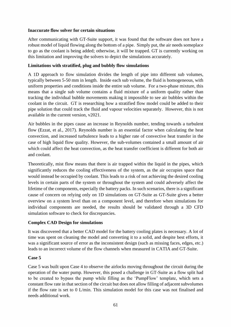
61

Inaccurate flow solver for certain situations

After communicating with GT-Suite support, it was found that the software does not have a

robust model of liquid flowing along the bottom of a pipe. Simply put, the air needs someplace

to go as the coolant is being added; otherwise, it will be trapped. GT is currently working on

this limitation and improving the solvers to depict the simulations accurately.

Limitations with stratified, plug and bubbly flow simulations

A 1D approach to flow simulation divides the length of pipe into different sub volumes,

typically between 5-50 mm in length. Inside each sub volume, the fluid is homogeneous, with

uniform properties and conditions inside the entire sub volume. For a two-phase mixture, this

means that a single sub volume contains a fluid mixture of a uniform quality rather than

tracking the individual bubble movements making it impossible to see air bubbles within the

coolant in the circuit. GT is researching how a stratified flow model could be added to their

pipe solution that could track the fluid and vapour velocities separately. However, this is not

available in the current version, v2021.

Air bubbles in the pipes cause an increase in Reynolds number, tending towards a turbulent

flow (Ezzat, et al., 2017). Reynolds number is an essential factor when calculating the heat

convection, and increased turbulence leads to a higher rate of convective heat transfer in the

case of high liquid flow quality. However, the sub-volumes contained a small amount of air

which could affect the heat convection, as the heat transfer coefficient is different for both air

and coolant.

Theoretically, mist flow means that there is air trapped within the liquid in the pipes, which

significantly reduces the cooling effectiveness of the system, as the air occupies space that

would instead be occupied by coolant. This leads to a risk of not achieving the desired cooling

levels in certain parts of the system or throughout the system and could adversely affect the

lifetime of the components, especially the battery packs. In such scenarios, there is a significant

cause of concern on relying only on 1D simulations on GT-Suite as GT-Suite gives a better

overview on a system level than on a component level, and therefore when simulations for

individual components are needed, the results should be validated through a 3D CFD

simulation software to check for discrepancies.

Complex CAD Design for simulations

It was discovered that a better CAD model for the battery cooling plates is necessary. A lot of

time was spent on cleaning the model and converting it to a solid, and despite best efforts, it

was a significant source of error as the inconsistent design (such as missing faces, edges, etc.)

leads to an incorrect volume of the flow channels when measured in CATIA and GT-Suite.

Case 5

Case 5 was built upon Case 4 to observe the airlocks moving throughout the circuit during the

operation of the water pump. However, this posed a challenge in GT-Suite as a flow split had

to be created to bypass the pump while filling as the ‘PumpFlow’ template, which sets a

constant flow rate in that section of the circuit but does not allow filling of adjacent subvolumes

if the flow rate is set to 0 L/min. This simulation model for this case was not finalised and

needs additional work.

62

6 Conclusion Through this research, it was found that there is a potential in using 1D CFD techniques to

simulate the coolant-air interaction in a cooling system. As mentioned earlier, this study was

conducted only for the lower temperature battery cooling circuit, which was a limited part of

the complete circuit. Due to this, no concrete recommendations can be made for other parts of

the circuit, but general estimations and a trend can be obtained by viewing the results of this

thesis work.

The work done during this thesis can be used as an example of what is possible in GT-Suite

and how can filling simulations be carried out with GT-Suite. While this study provides a good

initial point for validation, further study is necessary to test additional parts of the circuit with

a different setup to obtain more accurate results, as suggested in chapter 7. This will ensure

repeatability in the technique and build upon the previously done work to provide quick

solutions to the otherwise cumbersome task of building a new circuit.

6.1 Research Question 1

How well does the 1D simulations of filling a cooling system in Gamma Technologies Suite

(GT-Suite) equal filling a cooling system in a test rig?

From the results, it was found that GT-Suite can replicate the behaviour observed during testing

at both the auxiliary and the Scania test rig with some differences compared to the results

obtained from the physical experiments. This difference can be reduced by fine-tuning the

model further (by using accurate information from different sensors, modelling the geometry

accurately and increasing the discretisation). Nevertheless, from the results, it was found that

GT-Suite does not have a robust model yet to accurately simulate the interaction of coolant and

air in certain parts of the circuit, as mentioned in section 4. GT is currently working on

improving their model in the successive versions of the software.


What limitations could unique BEV components impose on 1D simulations?

It was observed that upon the addition of the three cooling plates, the implicit solver in GT-

Suite struggled to converge, and the model failed to reach a steady-state solution for increasing

time in every case. This effect was especially pronounced in Case 3 and Case 4, upon the

addition of the mixing line and removing the T-Joint. It is suspected that the addition of these

components changed the overall dynamics of the circuit (an example of which is explained

with pressure drops in Test Run 2, Case 4) and increased the complexity of the geometry,

resulting in inaccurate results.

63


To observe where the air is trapped in the circuit during filling and how can it be removed?

Air traps were observed in both the auxiliary and the Scania test rig. GT-Suite accurately

simulated air traps in the auxiliary test rig and this was because the coolant never reached that

section of the circuit. However, this test rig was only built to understand the working of GT-

Suite and to understand the relationship between the flow rate and the air traps created.

In the Scania test rig, small air traps were observed in Case 3 and Case 4 during filling. Case 5

focuses explicitly on deaeration, and it was found that the static line should have an increasing

angle with respect to the mixing line throughout its length to allow more air bubbles to escape

the circuit.

Different flow rates affect the deaeration and should be studied in detail to have a more robust

understanding of the behaviour of the fluid flowing through the circuit as suggested in section

7 as the experimental results showed that it is possible to have better deaeration at lower speeds

of the coolant pump.

Alternative methods were discovered theoretically, however, not performed experimentally.

These methods have been listed in section 7.

6.4 Research Contribution

1. This thesis work will help in increasing simulation done in R&D and reduce the

computation time it takes to perform simulations.

Currently, detailed 1D CFD simulations are limited to some components and only a few

departments within Scania. 1D CFD simulations on GT-Suite are easier and quicker to

perform than on 3D CFD software such as StarCCM+ or ANSA. 1D simulations can

allow the testing and design of the entire system as well as component level to some

extent to go hand in hand without delays.

2. Shorter lead time to launch BEV Trucks to reduce the carbon footprint of Scania’s

customers

The automotive industry is quickly racing towards implementing sustainable solutions,

including a rapid shift towards BEVs to reduce the carbon footprint, which can be

avoided if these trucks are brought into the market quicker. This thesis contributes to

three Sustainable Development Goals (United Nations, 2015):

64

• By 2030, upgrade infrastructure and

retrofit industries to make them

sustainable, with increased resource-use

efficiency and greater adoption of clean

and environmentally sound technologies

and industrial processes.

• Enhance scientific research, upgrade the

technological capabilities of industrial

sectors in all countries by 2030,

encouraging innovation and

substantially increasing the number of

research and development workers and

public, private research and

development spending

• By 2030, provide access to safe,

affordable, accessible, and sustainable

transport systems for all, improving road

safety, notably by expanding public

transport.

• By 2030, reduce the adverse per capita

environmental impact of cities,

including paying special attention to air

quality.

• Improve education, awareness-raising

and human and institutional capacity on

climate change mitigation, adaptation,

impact reduction and early warning.

• Integrate climate change measures into

strategies and planning.

3. Decreases the number and iterations of physical prototypes

1D CFD simulations can simulate the flow of coolant in the test rig instead of

manufacturing prototypes of the actual test rig. This provides cost and time-saving

opportunities and simultaneously avoids waste generation. Furthermore, it also

decreases the need for labour and allows for better resource optimisation

65

4. Less physical iterations required to a design approved (reduces labour, waste, and

resource optimisation)

A skeletal circuit with essential components can be designed on GT-Suite, and

additional components can be added to the circuit to make it more complex, eventually

including the entire cooling circuit.

66

7 Future work This thesis concludes with a validation that was carried out between the experimental testing

and the 1D CFD filling simulation using GT-Suite. The majority of the data, such as flowrates,

circuit geometry, was obtained from the test rig at Scania with additional input from GT-Suite

support staff to assist with the course of the work. This thesis work also provided insights into

the limitations in the entities used, and future research work can be to look into the limitations

and finding alternate strategies for 1D simulations.

The following is a list of recommendations from the authors of this thesis for an alternative

approach when reproducing the results of this thesis.

• A release valve that opens when air pressure exceeds a set threshold, especially before

pumps. It was observed that larger air traps on passing through the pump are dispersed

as small air bubbles throughout the circuit. This behaviour of the pump splitting the

large bubble into multiple smaller bubbles could be studied further in detail.

• The battery cooling plates and the mixing line in the test rig could be made of a much

more transparent material instead of aluminium to observe the air and coolant

interaction for testing.

• The battery cooling plates could be turned around, and the coolant flow could be against

gravity as it was very challenging to remove the coolant from the bottom plate once

filled.

• Due to difficulties in emptying the plates after every test run, a value of 7 seconds was

added to every subsequent filling test run; however, this was a very rough

approximation of the time it could take for different flow rates.

• The coolant could be filled from the lowest point in the circuit that is from the bottom-

most cooling plate instead. During this thesis work, it was observed that GT-Suite has

difficulties simulating the flow of coolant when it enters the circuit from two inlets.

Many times, this resulted in the implicit solver not converging, thereby reducing the

reliability of the results.

Scope of improvement

In order to obtain better simulation results from the circuit, the following areas of opportunities

were seen but could not be addressed either due to the limitation of time or due to limitations

of the software at its current version.

• A finer discretisation of components like flow channels inside the mixing line and

battery cooling plates in GEM3D will improve the accuracy of the results. The majority

of the components in this thesis work were set with a discretisation length of 30-40 mm.

• Additional fine-tuning of the 1D circuit diagrams can be done in GT-ISE to make it

easier to understand and have more data regarding the pressure drops at each section in

the battery cooling plates.

• An additional pressure sensor and flowmeter can be installed at the inlet to obtain the

data accurately. Due to the absence of a pressure sensor at the inlet, it was challenging

67

to find out the pressure of the coolant being pumped into the system; instead, the

volumetric flow rate for each case was experimentally found out and measured through

the flowmeter installed in a different section of the circuit.

• Alternate theories and hypotheses to analyse the pressure drops in cooling rods and the

battery cooling plates can be done

• Correlation between air traps and Reynolds number (turbulent or laminar flow).

• A vacuum pump can be used to remove air in production, but it is not used during

testing at test rigs. A vacuum pump should be introduced to the test rigs to prevent

airlocks, mist flow and observe this behaviour in a much more detailed manner.

68

References Astakhov, V. P. & Joksch, S., 2012. Environmentally friendly near-dry machining of metals.

In: Metalworking Fluids (MWFs) for Cutting and Grinding. s.l.:Woodhead Publishing, pp.

135-200.

BorgWarner, 2020. BorgWarner’s New High-Voltage Coolant Heaters are the First Choice

of Global OEMs, s.l.: s.n.

Burak, S., Tolga, E. & Omer, T., 2017. Does a battery-electric truck make a difference? –

Life cycle emissions, costs, and externality analysis of alternative fuel-powered Class 8

heavy-duty trucks in the United States. Journal of Cleaner Production, Volume 141, pp. 110-

121.

Cengel, Y. A., 2011. Heat and Mass Transfer.. s.l.:McGraw-Hill Education.

Chastain, J., 2006. Internal Combustion Engine Cooling Strategies: Theory and Test, s.l.: s.n.

Cheremisinoff, N. P. & Gupta, R., 1983. Handbook of fluids in motion. s.l.:Ann Arbor

Science.

Cruz, D. A., Coelho, P. M. & Alves, M. A., 2012. A Simplified Method for Calculating Heat

Transfer Coefficients and Friction Factors in Laminar Pipe Flow of Non-Newtonian Fluids.

Journal Of Heat Transfer-Transactions Of The Asme, 134(9).

Dinakar, P. & Rajeeve, G., 2016. Modelling and Simulation of Cooling , s.l.: Chalmers

Univeristy of Technology.

Evans Cooling Systems Australasia, 2016. DON’T BE FOOLED BY THE ‘AIR LOCK’.

[Online]

Available at: https://www.evanscoolants.com.au/news/dont-be-fooled-by-the-air-lock/

[Accessed 18 March 2021].

Ezzat, A. W., Abdullah, N. N. & Ghashim, S. L., 2017. Effect of Air Bubbles on Heat

Transfer Coefficient in Turbulent Convection Flow. Journal of Engineering, 23(1).

Feng, X. et al., 2018. Thermal runaway mechanism of lithium ion battery for electric

vehicles: A review. Energy Storage Materials, Volume 10, pp. 246-267.

Gamma Technologies, 2020. GT-Suite User Manual, s.l.: s.n.

Gamma Technologies, n.d. GEM3D Preprocessor. [Online]

Available at: https://www.gtisoft.com/gt-suite/productivity-tools/gem3d-preprocessor/

[Accessed 10 April 2021].

Gamma Technologies, n.d. GT-ISE (Integrated Simulation Environment). [Online]

Available at: https://www.gtisoft.com/gt-suite/productivity-tools/gt-ise-integrated-simulation-

environment/


Gamma Technologies, n.d. GT-POST. [Online]

Available at: https://www.gtisoft.com/gt-suite/productivity-tools/gt-ise-integrated-simulation-

69

environment/


Gamma Technologies, n.d. GT-SPACECLAIM. [Online]

Available at: https://www.gtisoft.com/gt-suite/productivity-tools/gt-spaceclaim-cad-model-

building-and-preparation/


Gao, Q. et al., 2019. An experimental investigation of refrigerant emergency spray on cooling

and oxygen suppression for overheating power battery. Journal of Power Sources, Volume

415, pp. 33-43.

Hu, X. et al., 2020. Battery warm-up methodologies at subzero temperatures for automotive

applications: Recent advances and perspectives. Progress in Energy and Combustion Science,

Volume 77.

International Transport Forum, 2017. ITF Transport Outlook, s.l.: OECD/ITF.

Jaewan, K., Jinwoo, O. & Hoseong, L., 2019. Review on battery thermal management system

for electric vehicles. Applied Thermal Energy, Volume 149, pp. 192-212.

Jarrett, A. & Kim, Y., 2011. Design optimization of electric vehicle battery cooling plates for

thermal performance. Journal of Power Sources, 196(23), pp. 10359-10368.

Kakaç, S., Liu, H. & Pramuanjaroenkij, A., 2002. Heat Exchangers. 3rd ed. Boca Raton:

CRC Press.

Kane, M., 2017. Efficiency Compared: Battery-Electric 73%, Hydrogen 22%, ICE 13%, s.l.:

s.n.

Lajunen, A., Yang, Y. & Emadi, A., 2018. Recent Developments in Thermal Managementof

Electrified Powertrains. TRANSACTIONS ON VEHICULAR TECHNOLOGY, 67(12).

Liimatainen, H., van Vliet, O. & Aplyn, D., 2019. The potential of electric trucks – An

international commodity-level analysis. Applied Energy, Volume 236, pp. 804-814.

Li, J. & Zhu, Z., 2014. Battery Thermal Management Systems of , s.l.: Chalmers Univeristy of

Technology.

Lin, W. & Sundén, B., 2010. Vehicle Cooling Systems for Reducing Fuel Consumption and

Carbon Dioxide: Literature Survey. SAE Technical Paper.

Miao, Y., Hynan, P., von Jouanne, A. & Yokochi, A., 2019. Current Li-Ion Battery

Technologies in Electric Vehicles and Opportunities for Advancements. Energies, 12(6), pp.

1074-1094.

Mulholland, E. et al., 2018. The long haul towards decarbonising road freight – A global

assessment to 2050. Applied Energy, Volume 216, pp. 678-693.

OARDS Automotive Hub, 2020. Top 5 Causes of Car Overheating: Read This and Save

Your Engine!. [Online]

Available at: https://oards.com/causes-of-car-overheating/

[Accessed 18 March 2021].

70

Palmgren, J. & Hjälm Wallborg, M., 2015. Improving engine oil cooler , s.l.: s.n.

Peters, A. et al., 2012. Electric mobility concepts and their significance for the economy,

society and the environment, s.l.: s.n.

Prudhvi, G., Vinay, G. & Suresh Babu, G., 2013. Cooling Systems in Automobiles & Cars.

International Journal of Engineering and Advanced Technology (IJEAT), 2(1).

Q.Xin & C.F.Pinzon, 2014. Improving the environmental performance of heavy-duty vehicles

and engines: key issues and system design approaches. s.l.:s.n.

Rapp, B. E., 2017. Fluids. In: Microfluidics: Modeling, Mechanics and Mathematics.

s.l.:Elsevier, pp. 243-263.

Rudravajhala, M., 2018. Evaluation of 1D and 3D CFD Simulation, Gothenburg:

CHALMERS UNIVERSITY OF TECHNOLOGY.

Sato, N., 2001. Thermal behavior analysis of lithium-ion batteries for electric and hybrid

vehicles. Journal of Power Sources, 99(1-2), pp. 70-77.

Śliwiński, K. & Szramowiat, M., 2018. Development of cooling systems for internal

combustion engines in the light of the requirements of modern drive systems. IOP

Conference Series: Materials Science and Engineering, 421(4).

Stringer, D. & Park, K., 2020. Why Building an Electric Car Is So Expensive, For Now, s.l.:

Bloomberg Green.

Teboho, C. et al., 2018. Thermal Conductivity of Graphite-Based Polymer Composites.

IntechOpen.

Transport & Environment, 2017. Electric truck's contribution to freight decarbonisation, s.l.:

s.n.

United Nations, 2015. The 17 Goals. [Online]

Available at: https://sdgs.un.org/es/goals

[Accessed 2 July 2021].

White, F. M., 2010. Fluid Mechanics. s.l.:McGraw-Hill Education.

Wolfram, P. & Lutsey, N., 2016. Electric vehicles: Literature review of technology costs and

carbon emissions, s.l.: International Council on Clean Transportation.

X-Engineer, 2021. [Online]

Available at: https://x-engineer.org/automotive-engineering/vehicle/electric-

vehicles/anatomy-of-a-battery-electric-vehicle-bev/

[Accessed 8 June 2021].

Xylem Applied Water Systems, 2015. Pump cavitation and how to avoid it, s.l.: s.n.

Zhang, T., 2020. When to Use 1D Vs. 3D Simulation. [Online]

Available at: https://blog.softinway.com/when-to-use-1d-vs-3d-simulation/

Zimmerman, A. H. & Quinzio, M. V., 2010. Lithium Plating in Lithium-Ion Cells. s.l., The

Aerospace Corporation.

Suite - DiVA-Portal

Documents