Subsample ignorable likelihood for accelerated failure time models with missing predictors

Lifetime Data AnalDOI 10.1007/s10985-014-9304-x

Subsample ignorable likelihood for accelerated failuretime models with missing predictors

Nanhua Zhang · Roderick J. Little

Received: 19 April 2012 / Accepted: 16 July 2014© Springer Science+Business Media New York 2014

Abstract Missing values in predictors are a common problem in survival analysis.In this paper, we review estimation methods for accelerated failure time models withmissing predictors, and apply a new method called subsample ignorable likelihood(IL) Little and Zhang (J R Stat Soc 60:591–605, 2011) to this class of models. Theapproach applies a likelihood-based method to a subsample of observations that arecomplete on a subset of the covariates, chosen based on assumptions about the missingdata mechanism. We give conditions on the missing data mechanism under which thesubsample IL method is consistent, while both complete-case analysis and ignorablemaximum likelihood are inconsistent. We illustrate the properties of the proposedmethod by simulation and apply the method to a real dataset.

Keywords Missing covariates · Mortality · Non-ignorable missingness · Partiallikelihood

Electronic supplementary material The online version of this article (doi:10.1007/s10985-014-9304-x)contains supplementary material, which is available to authorized users.

N. Zhang (B)Division of Biostatistics & Epidemiology, Cincinnati Children’s Hospital Medical Center,Cincinnati, OH 45229, USAe-mail: [email protected]

R. J. LittleDepartment of Biostatistics, School of Public Health, University of Michigan,Ann Arbor, MI 48109-2029, USAe-mail: [email protected]

123

N. Zhang, R. J. Little

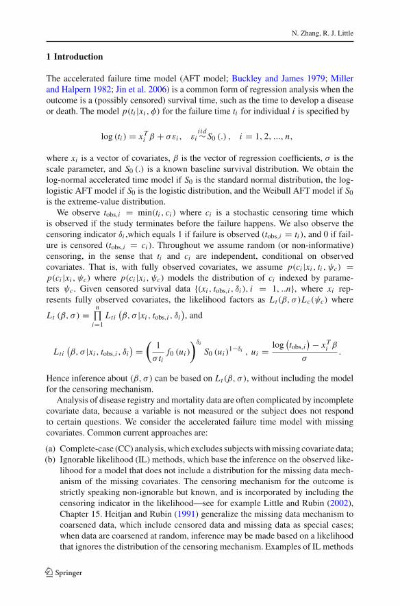
1 Introduction

The accelerated failure time model (AFT model; Buckley and James 1979; Millerand Halpern 1982; Jin et al. 2006) is a common form of regression analysis when theoutcome is a (possibly censored) survival time, such as the time to develop a diseaseor death. The model p(ti |xi , φ) for the failure time ti for individual i is specified by

log (ti ) = xTi β + σεi , εi

i id∼ S0 (.) , i = 1, 2, ..., n,

where xi is a vector of covariates, β is the vector of regression coefficients, σ is thescale parameter, and S0 (.) is a known baseline survival distribution. We obtain thelog-normal accelerated time model if S0 is the standard normal distribution, the log-logistic AFT model if S0 is the logistic distribution, and the Weibull AFT model if S0is the extreme-value distribution.

We observe tobs,i = min(ti , ci ) where ci is a stochastic censoring time whichis observed if the study terminates before the failure happens. We also observe thecensoring indicator δi ,which equals 1 if failure is observed (tobs,i = ti ), and 0 if fail-ure is censored (tobs,i = ci ). Throughout we assume random (or non-informative)censoring, in the sense that ti and ci are independent, conditional on observedcovariates. That is, with fully observed covariates, we assume p(ci |xi , ti , ψc) =p(ci |xi , ψc) where p(ci |xi , ψc) models the distribution of ci indexed by parame-ters ψc. Given censored survival data {(xi , tobs,i , δi ), i = 1, ..n}, where xi rep-resents fully observed covariates, the likelihood factors as Lt (β, σ )Lc(ψc) where

Lt (β, σ ) =n∏

i=1Lti

(β, σ |xi , tobs,i , δi

), and

Lti(β, σ |xi , tobs,i , δi

) =(

1

σ tif0 (ui )

)δi

S0 (ui )1−δi , ui = log

(tobs,i

) − xTi β

σ.

Hence inference about (β, σ ) can be based on Lt (β, σ ), without including the modelfor the censoring mechanism.

Analysis of disease registry and mortality data are often complicated by incompletecovariate data, because a variable is not measured or the subject does not respondto certain questions. We consider the accelerated failure time model with missingcovariates. Common current approaches are:

(a) Complete-case (CC) analysis, which excludes subjects with missing covariate data;(b) Ignorable likelihood (IL) methods, which base the inference on the observed like-

lihood for a model that does not include a distribution for the missing data mech-anism of the missing covariates. The censoring mechanism for the outcome isstrictly speaking non-ignorable but known, and is incorporated by including thecensoring indicator in the likelihood—see for example Little and Rubin (2002),Chapter 15. Heitjan and Rubin (1991) generalize the missing data mechanism tocoarsened data, which include censored data and missing data as special cases;when data are coarsened at random, inference may be made based on a likelihoodthat ignores the distribution of the censoring mechanism. Examples of IL methods

123

Subsample ignorable likelihood

include ignorable maximum likelihood (IML; Meng and Schenker 1999; Cho andSchenker 1999; Lipsitz and Ibrahim 1996a,b), Bayesian inferences (Chen et al.2002; Bedrick et al. 2000), and multiple imputation (Giorgi et al. 2008; White andRoyston 2009),

(c) Non-ignorable modeling methods, which jointly model the variables and the miss-ing data mechanism for the covariates (Hemming and Hutton 2010; Herring et al.2002). This approach is less common in practice, because it is difficult to specifythe model for the missing data mechanism correctly, and problems with identifyingthe parameters [Little and Rubin (2002), Ch. 15].

IL methods have the advantage of retaining all data, but they assume that the missingdata are missing at random (MAR), in the sense that the missingness of the covariatesdoes not depend on the missing values, after conditioning on the observed data (Rubin1976; Little and Rubin 2002). CC analysis involves a loss of information but hasthe advantage of yielding valid inference when the missingness depends only on thecovariates, but not on the failure time. Little and Zhang (2011) provide a formaljustification based on partial likelihood ideas.

In this article, we apply the Little and Zhang (2011) subsample ignorable likelihoodmethods to the accelerated failure time model (SILAFT). The method mitigates theinformation loss of CC analysis while still allowing missingness of some covariates todepend on their underlying values, a nonignorable mechanism where IL methods aresubject to bias. The key idea is to partition the covariates into three sets—one set (sayZ ) fully observed, one set (say W ) for which the missingness is assumed to dependon covariates (including W ) but not on the failure time, and one set (say X ) for whichthe missingness are assumed MAR in the subsample of cases with W fully observed.The proposed SILAFT methods apply an IL method to the subsample of case withW fully observed. Particular forms of SILAFT methods include ignorable maximumlikelihood, Bayesian inference, and multiple imputation. Conditions formalized inSect. 4 indicate that SILAFT gives valid estimates in circumstances where both CCand IL methods are biased.

Section 2 presents a motivating problem based on data from the National Longitudi-nal Mortality Study (NLMS), where the AFT model is applied to study the relationshipbetween mortality and education and income, adjusting for race, gender, and maritalstatus. In this application, gender and age are fully observed, but the other variableshave missing values; it was thought that missingness of education, race, and maritalstatus was at random, but missingness of household income was likely to depend onincome. In this example, Z consists of age and gender, W consists of income andX consists of education, race and marital status. The SILAFT methods apply an ILmethod to the subsample of cases with income observed.

Section 3 presents the proposed SILAFT method and describes conditions on themissing data mechanism under which it gives consistent estimates, but both IL andCC analyses are biased. We illustrate the properties of the SILAFT methods andalternatives in Sect. 4, using simulation studies. In Sect. 5, we apply the method tothe motivating data from the NLMS (Sorlie et al. 1995). We conclude with somediscussion in Sect. 6.

123

N. Zhang, R. J. Little

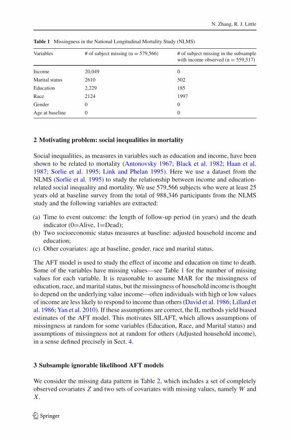
Table 1 Missingness in the National Longitudinal Mortality Study (NLMS)

Variables # of subject missing (n = 579,566) # of subject missing in the subsamplewith income observed (n = 559,517)

Income 20,049 0

Marital status 2610 502

Education 2,229 185

Race 2124 1997

Gender 0 0

Age at baseline 0 0

2 Motivating problem: social inequalities in mortality

Social inequalities, as measures in variables such as education and income, have beenshown to be related to mortality (Antonovsky 1967; Black et al. 1982; Haan et al.1987; Sorlie et al. 1995; Link and Phelan 1995). Here we use a dataset from theNLMS (Sorlie et al. 1995) to study the relationship between income and education-related social inequality and mortality. We use 579,566 subjects who were at least 25years old at baseline survey from the total of 988,346 participants from the NLMSstudy and the following variables are extracted:

(a) Time to event outcome: the length of follow-up period (in years) and the deathindicator (0=Alive, 1=Dead);

(b) Two socioeconomic status measures at baseline: adjusted household income andeducation;

(c) Other covariates: age at baseline, gender, race and marital status.

The AFT model is used to study the effect of income and education on time to death.Some of the variables have missing values—see Table 1 for the number of missingvalues for each variable. It is reasonable to assume MAR for the missingness ofeducation, race, and marital status, but the missingness of household income is thoughtto depend on the underlying value income—often individuals with high or low valuesof income are less likely to respond to income than others (David et al. 1986; Lillard etal. 1986; Yan et al. 2010). If these assumptions are correct, the IL methods yield biasedestimates of the AFT model. This motivates SILAFT, which allows assumptions ofmissingness at random for some variables (Education, Race, and Marital status) andassumptions of missingness not at random for others (Adjusted household income),in a sense defined precisely in Sect. 4.

3 Subsample ignorable likelihood AFT models

We consider the missing data pattern in Table 2, which includes a set of completelyobserved covariates Z and two sets of covariates with missing values, namely W andX .

123

Subsample ignorable likelihood

Table 2 General missing data structure for Sect. 3

Pattern Observation, i zi wi xi (ti , δi ) Rwi Rxi

1 i =1,…,m√ √ √ √

uw ux

2 i = m+1,…,m + r√ √

x√

uw ux

3 i = m + r+1,…,n√

x ?√

uw ux or ux

Key:√

denotes observed, x denotes at least one entry missing, ? denotes observed or missing

The columns Rwi and Rxi represents vectors of response indicators for wi and xi ,the values of W and X for unit i , with entries 1 if a variable is observed and 0 if avariable is missing. To describe missing data patterns for a set of variables (say v), itis convenient to write uv = (1, ..., 1) to denote a vector of 1’s of the same length asthe vector v, and uv to denote a vector of 0’s and 1’s of the same length as v for whichat least one entry is zero. In Table 2, Rwi = uw, Rx = ux for the complete cases inPattern 1, Rwi = uw, Rx = ux for the cases in Pattern 2, where W is fully observedand X has at least one missing value, and Rwi = uw for the cases in Pattern 3, whereW has at least one missing value. The pattern of missing values will typically vary forcases within these three sets, but we do not need to distinguish them for the presentdiscussion. Interest concerns the parameters φ of the distribution of (tobs,i , δi ) given(zi , wi , xi ), say p((tobs,i , δi )|zi , wi , xi , φ). We propose SILAFT, which discards datain Pattern 3 and applies an IL method to the subsample of cases in Patterns 1 and 2with both Z and W observed. The division of covariates into W and X for SILAFTis determined by assumptions about the missing data mechanism. Specifically, themethod is valid under the following three assumptions:

(a) Covariate missingness of W : The probability that W is fully observed dependsonly on the covariates and not the censoring or failure times (ti , ci ), that is:

p(Rwi = uw|zi , wi , xi , ti , ci , ψw

) = p(Rwi = uw|zi , wi , xi , ψw

)for all (ti , ci )

(1)(b) Subsample MAR of X : Missingness of X is MAR within the subsample of cases

for which W is fully observed, that is:

p(Rxi |zi , wi , xi , ti , ci , Rwi = uw,Ψx ) =p(Rxi |zi , wi , xobs,i , tobs,i , δi , Rwi = uw,ψx ) for all xmis,i , tmis,i , ci ,

(2)where tmis,i is the survival time for censored case i , and xobs,i , xmis,i are theobserved and missing components of xi , respectively.

(c) The censored survival times are coarsened at random (Heitjan and Rubin 1991)within the subsample for cases for which W is fully observed, that is:

p(ci |ti , zi , wi , xi , ψc) = p(ci |zi , wi , xobs,i , ψc) for all ti , xmis,i , (3)

where p(ci |ti , zi , wi , xi , ψc) is a model for the stochastic censoring times indexed byparameters ψc. The validity of SILAFT under (1)–(3) is obtained by combining the

123

N. Zhang, R. J. Little

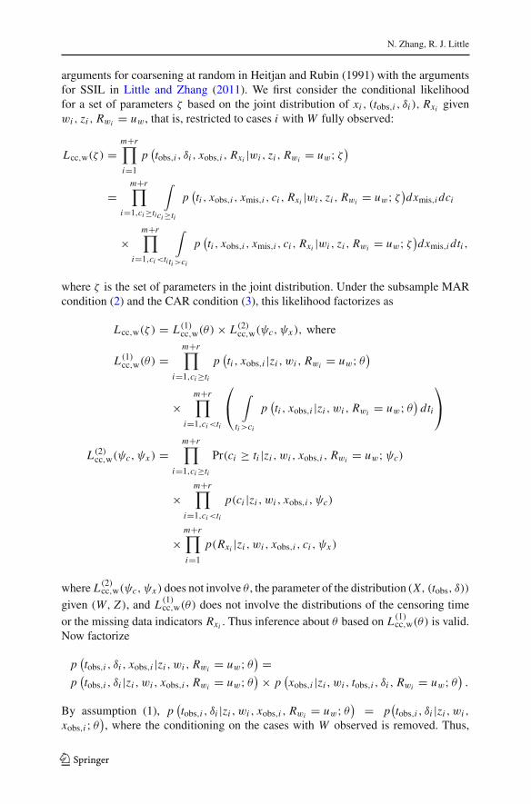
arguments for coarsening at random in Heitjan and Rubin (1991) with the argumentsfor SSIL in Little and Zhang (2011). We first consider the conditional likelihoodfor a set of parameters ζ based on the joint distribution of xi , (tobs,i , δi ), Rxi givenwi , zi , Rwi = uw, that is, restricted to cases i with W fully observed:

Lcc,w(ζ ) =m+r∏

i=1

p(tobs,i , δi , xobs,i , Rxi |wi , zi , Rwi = uw; ζ )

=m+r∏

i=1,ci ≥ti

∫

ci ≥ti

p(ti , xobs,i , xmis,i , ci , Rxi |wi , zi , Rwi = uw; ζ )dxmis,i dci

×m+r∏

i=1,ci<ti

∫

ti>ci

p(ti , xobs,i , xmis,i , ci , Rxi |wi , zi , Rwi = uw; ζ )dxmis,i dti ,

where ζ is the set of parameters in the joint distribution. Under the subsample MARcondition (2) and the CAR condition (3), this likelihood factorizes as

Lcc,w(ζ ) = L(1)cc,w(θ)× L(2)cc,w(ψc, ψx ), where

L(1)cc,w(θ) =m+r∏

i=1,ci ≥ti

p(ti , xobs,i |zi , wi , Rwi = uw; θ)

×m+r∏

i=1,ci<ti

⎛

⎝∫

ti>ci

p(ti , xobs,i |zi , wi , Rwi = uw; θ) dti

⎞

⎠

L(2)cc,w(ψc, ψx ) =m+r∏

i=1,ci ≥ti

Pr(ci ≥ ti |zi , wi , xobs,i , Rwi = uw;ψc)

×m+r∏

i=1,ci<ti

p(ci |zi , wi , xobs,i , ψc)

×m+r∏

i=1

p(Rxi |zi , wi , xobs,i , ci , ψx )

where L(2)cc,w(ψc, ψx ) does not involve θ , the parameter of the distribution (X, (tobs, δ))

given (W, Z), and L(1)cc,w(θ) does not involve the distributions of the censoring timeor the missing data indicators Rxi . Thus inference about θ based on L(1)cc,w(θ) is valid.Now factorize

p(tobs,i , δi , xobs,i |zi , wi , Rwi = uw; θ) =

p(tobs,i , δi |zi , wi , xobs,i , Rwi = uw; θ) × p

(xobs,i |zi , wi , tobs,i , δi , Rwi = uw; θ) .

By assumption (1), p(tobs,i , δi |zi , wi , xobs,i , Rwi = uw; θ) = p

(tobs,i , δi |zi , wi ,

xobs,i ; θ), where the conditioning on the cases with W observed is removed. Thus,

123

Subsample ignorable likelihood

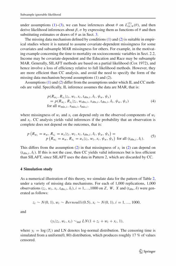
under assumptions (1)–(3), we can base inferences about θ on L(1)cc,w(θ), and thenderive likelihood inferences about β, σ by expressing them as functions of θ and thensubstituting estimates or draws of θ as in Sect. 3.

The missing data mechanism defined by conditions (1) and (2) is suitable in empir-ical studies where it is natural to assume covariate-dependent missingness for somecovariates and subsample MAR missingness for others. For example, in the motivat-ing example concerning the time to mortality on socioeconomic variables in Sect. 2.2,Income may be covariate-dependent and the Education and Race may be subsampleMAR. Generally, SILAFT methods are based on a partial likelihood (Cox 1972), andhence involve a loss of efficiency relative to full likelihood methods. However, theyare more efficient than CC analysis, and avoid the need to specify the form of themissing data mechanism beyond assumptions (1) and (2).

Assumptions (1) and (2) differ from the assumptions under which IL and CC meth-ods are valid. Specifically, IL inference assumes the data are MAR, that is:

p(Rwi , Rxi |zi , wi , xi , tobs,i , δi , ψw,ψx )

= p(Rwi , Rxi |zi , wobs,i , xobs,i , tobs,i , δi , ψw,ψx )

for all wmis,i , xmis,i , tmis,i .

(4)

where missingness of wi and xi can depend only on the observed components of wi

and xi . CC analysis yields valid inferences if the probability that an observation iscomplete does not depend on the outcomes, that is:

p(Rwi = uw, Rxi = ux |zi , wi , xi , tobs,i , δi , ψw,ψx

) =p

(Rwi = uw, Rxi = ux |zi , wi , xi , ψw,ψx

)for all (tobs,i , δi ).

(5)

This differs from the assumption (2) in that missingness of xi in (2) can depend on(tobs,i , δi ). If this is not the case, then CC yields valid inferences but is less efficientthan SILAFT, since SILAFT uses the data in Pattern 2, which are discarded by CC.

4 Simulation study

As a numerical illustration of this theory, we simulate data for the pattern of Table 2,under a variety of missing data mechanisms. For each of 1,000 replications, 1,000observations (zi , wi , xi , tobs,i , δi ), i = 1,…,1000 on Z , W, X and (tobs, δ) were gen-erated as follows:

zi ∼ N (0, 1), wi ∼ Bernoulli(0.5), xi ∼ N (0, 1), i = 1, ..., 1000,

and

(yi |zi , wi , xi ) ∼ind L N (1 + zi + wi + xi , 1),

where yi = log (Ti ) and LN denotes log-normal distribution. The censoring time issimulated from a uniform(0, 80) distribution, which produces roughly 17 % of valuescensored.

123

N. Zhang, R. J. Little

Table 3 Missing data mechanisms generated in the simulations

Mechanisms α(w)0 α

(w)z α

(w)w α

(w)x α

(w)t α

(x)0 α

(x)z α

(x)w α

(x)x α

(x)t

I: All valid −1 1 0 0 0 −1 1 0 0 0

II: CC valid −1.7 1 1 1 0 −1.7 1 1 1 0

III: IL valid −4 1 0 0 025 −2.5 1 1 0 0.25

IV: SILAFT valid −1.5 1 1 0 0 −3.5 1 1 0 0.25

Missing value of W and X are generated based on the following logistic models:

logit(P(Rwi = 0|zi , wi , xi , (ti , δi ))

) = α(w)0 + α

(w)z zi + α

(w)w wi + α

(w)x xi + α

(w)t ti

logit(P(Rxi = 0|Rwi = 1, zi , wi , xi , (ti , δi ))

) = α(x)0 + α

(x)z zi + α

(x)w wi + α

(x)x xi + α

(x)t ti

In particular, for the four missing data mechanisms:I: Missingness of W = f (Z), Missingness of X = f (Z|W observed), all four methods are valid;II: Missingness of W = f (Z ,W, X), Missingness of X = f (Z,W,X|W observed), only CC valid;III: Missingness of W = f (Z), Missingness of X = f (Z,W|W observed), only IL valid;IV: Missingness of W = f (Z ,W, (t, δ)), Missingness of X = f (Z ,W, (t, δ),W observed), only SILAFTvalid

Missing values of W and X were then generated from the following two logisticmodels:

logit(P(Rwi = 0|zi , wi , xi , tobs,i , δi , ψw)

)

= ψ(w)0 + ψ(w)z zi + ψ(w)w wi + ψ(w)x xi + ψ

(w)t ti

logit(P(Rxi = 0|Rwi = 1, zi , wi , xi , tobs,i , δi , ψx )

)

= ψ(x)0 + ψ(x)z zi + ψ(x)w wi + ψ(x)x xi + ψ

(x)t ti

with xi fully observed when wi is missing.For the missing data generation schemes above, CC analysis is valid if both ψ(w)t

andψ(x)t are zero; IL is valid ifψ(w)w , ψ(w)x andψ(x)x are zero; SILAFT is valid ifψ(w)t

and ψ(x)x are zero. Four missing data mechanisms were created using different setsof values for the regression coefficients such that, in mechanism (I) all three methods(CC, IL and SILAFT) are consistent, while in mechanisms (II), (III) and (IV), just oneof the three methods is valid. The simulation setup is summarized in Table 3.

These missing data mechanisms all generate approximately 30 and 20 % valuesmissing in W and X , respectively.

Four specific versions of the methods are applied to estimate the regression coeffi-cients:

(1) CC analysis, using a AFT model assuming a log normal distribution for yi ;(2) IML: ignorable ML for the whole dataset;(3) SILAFT: IML for the subsample with W observed;(4) Before deletion (BD): least squares estimates from the regression BD, as a bench-

mark method.

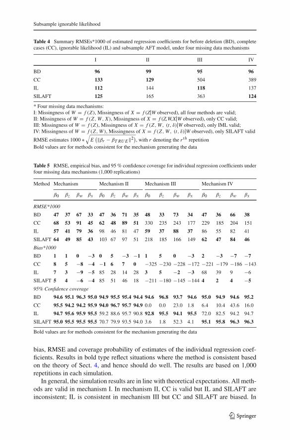
For each method, Table 4 summarizes the root mean squared errors (RMSEs) of esti-mates of all the regression coefficients, and Tables 5 reports respectively the empirical

123

Subsample ignorable likelihood

Table 4 Summary RMSEs*1000 of estimated regression coefficients for before deletion (BD), completecases (CC), ignorable likelihood (IL) and subsample AFT model, under four missing data mechanisms

I II III IV

BD 96 99 95 96

CC 133 129 504 389

IL 112 144 118 137

SILAFT 125 165 363 124

* Four missing data mechanisms:I: Missingness of W = f (Z), Missingness of X = f (Z|W observed), all four methods are valid;II: Missingness of W = f (Z ,W, X), Missingness of X = f (Z,W,X|W observed), only CC valid;III: Missingness of W = f (Z), Missingness of X = f (Z ,W, (t, δ)|W observed), only IML valid;IV: Missingness of W = f (Z ,W ), Missingness of X = f (Z ,W, (t, δ)|W observed), only SILAFT valid

RMSE estimates 1000 ∗√

E(‖βr − βT RU E ‖2)

, with r denoting the r th repetitionBold values are for methods consistent for the mechanism generating the data

Table 5 RMSE, empirical bias, and 95 % confidence coverage for individual regression coefficients underfour missing data mechanisms (1,000 replications)

Method Mechanism Mechanism II Mechanism III Mechanism IV

β0 βz βw βx β0 βz βw βx β0 βz βw βx β0 βz βw βx

RMSE*1000

BD 47 37 67 33 47 36 71 35 48 33 73 34 47 36 66 38

CC 68 53 91 45 62 48 89 51 330 235 243 177 229 185 204 151

IL 57 41 79 36 98 46 81 47 59 37 88 37 86 55 82 41

SILAFT 64 49 85 43 103 67 97 51 218 185 166 149 62 47 84 46

Bias*1000

BD 1 1 0 −3 0 5 −3 −1 1 5 0 −3 2 −3 −7 −7

CC 8 5 −8 −4 −1 6 7 0 −325 −230 −228 −172 −221 −179 −186 −143

IL 7 3 −9 −5 85 28 14 28 3 5 −2 −3 68 39 9 −6

SILAFT 5 4 −6 −4 85 51 46 18 −211 −180 −145 −144 4 2 4 −5

95% Confidence coverage

BD 94.6 95.1 96.3 95.0 94.9 95.5 95.4 94.4 94.6 96.8 93.7 94.6 95.0 94.9 94.6 95.2

CC 95.5 94.2 94.2 95.9 94.0 96.7 95.7 94.9 0.0 0.0 23.0 1.8 6.4 10.4 43.6 16.0

IL 94.7 95.6 95.9 95.5 59.2 88.6 95.7 90.8 92.8 95.5 94.1 95.5 72.0 82.5 94.2 94.7

SILAFT 95.0 95.5 95.5 95.5 70.7 79.9 93.5 94.0 3.6 1.8 52.3 4.1 95.1 95.8 96.3 96.3

Bold values are for methods consistent for the mechanism generating the data

bias, RMSE and coverage probability of estimates of the individual regression coef-ficients. Results in bold type reflect situations where the method is consistent basedon the theory of Sect. 4, and hence should do well. The results are based on 1,000repetitions in each simulation.

In general, the simulation results are in line with theoretical expectations. All meth-ods are valid in mechanism I. In mechanism II, CC is valid but IL and SILAFT areinconsistent; IL is consistent in mechanism III but CC and SILAFT are biased. In

123

N. Zhang, R. J. Little

mechanism IV, SILAFT is consistent but CC and IL are inconsistent, and in this caseSILAFT has small empirical bias and generally performs best, except for some indi-vidual coefficients where the gain in efficiency of IL compensates for the bias of thatmethod. We now describe results in a bit more detail.

For mechanism I, all three methods yield consistent estimates, IL is best since itmakes full use of the data, CC is the worst since it discards the most information, andSILAFT lies between CC and IL, since it retains some incomplete cases and dropsothers.

For mechanism II, CC is valid and in general has the lowest RMSEs, while bothIL and SILAFT are biased. However, IL yield comparable or even smaller RMSEsthan CC for βz and βw, reflecting gains in efficiency that compensate for bias in theseparameter estimates.

For mechanism III, IL is the only valid method among the three, and is clearly thebest method. Both CC and SILAFT lead to biased estimates, as shown in Table 4, withSILAFT being better than CC since it is incorporates features of IL as a method.

In mechanism IV, SILAFT is valid while CC and IL are biased. The RMSEs fromSILAFT are generally the smallest, except that IL yields a smaller RMSE than SILAFTfor βw and βx .

In some of these situations, supporters of IL may note that it competes well withother methods, despite its theoretical inconsistency and the quite sizeable sample size.This becomes more pronounced when the proportion of missingness is larger (See theonline supplement for additional simulation studies when missingness proportionsare 50 and 30 % in W and X , respectively), and the biases in the IL methods arecompensated by improved precision. This suggests a degree of robustness for IL,which has the virtue of retaining all the data.

5 Application to motivating example

We now apply the proposed method to the data from the NLMS study that werepresented in Sect. 2. We fit log-linear models of the follow-up period (in years) on theadjusted household income (in 1,000 dollars per year) and education, adjusting forrace, gender, marital status, and baseline age (in years). Adjusted household incomedata are categorical in NLMS, and we use the median of the corresponding categoryas a proxy to the true adjusted household income. Education is dichotomized to begreater than high school and high school or less.

Age and gender are fully observed, whereas adjusted household income, educa-tion, race, and marital status are subject to missing data, with the percentage shownin Table 1. We assume covariate missingness for adjusted household income, givenevidence that people with high or low income are more likely to fail to report it, andwe assume subsample missingness at random for other covariates.

With those plausible assumptions, SILAFT on the subsample with adjusted house-hold income observed yields consistent estimates of the regression, whereas IL on thewhole sample may be biased. CC analysis is also valid since there is little evidenceto believe that missingness of covariates depends on the follow-up period; however,SILAFT is preferred over CC analysis since it uses more information in the incomplete

123

Subsample ignorable likelihood

Table 6 Estimates of AFT models: National Longitudinal Mortality Study

CC IL SILAFT

Parameter Estimate 95% C.I. Estimate 95% C.I. Estimate 95% C.I.

Intercept 7.020 (6.980, 7.061) 7.027 (6.987, 7.067) 7.019 (6.979, 7.059)

Education: >HS versusHS or less

0.154 (0.138, 0.170) 0.150 (0.135, 0.166) 0.155 (0.139, 0.171)

Adjusted income 0.077 (0.073, 0.080) 0.079 (0.075, 0.082) 0.077 (0.073, 0.080)

Race: black versus white −.195 (−.217,−.173) −.193 (−.214,−.170) −.195 (−.217,−.173)

Race: other versus white 0.149 (0.101, 0.198) 0.154 (0.106, 0.202) 0.149 (0.100, 0.197)

Gender: female versus male 0.590 (0.577, 0.604) 0.591 (0.578, 0.605) 0.591 (0.577, 0.604)

Marital status: marriedversus other

0.214 (0.199, 0.228) 0.210 (0.196, 0.224) 0.214 (0.199, 0.229)

Age at baseline −.072 (−.072,−.071) −.072 (−.072,−.071) −.072 (−.072,−.071)

C.I. credible interval.

cases than does CC analysis. WinBUGS code for implementing the SILAFT methodis provided in the online supplement.

The results of CC analysis, IL and SILAFT are shown in Table 6. All three methodsyield similar estimates because the missing proportions of the variables are small. TheIL method gives smaller standard errors than CC because it uses more sample than CC.SILAFT is a hybrid of CC and IL, yielding standard errors of SILAFT that lie betweenCC and IL. There is positive effect of adjusted household income and education, withsurvival time increasing as adjusted household income and education increases. Raceand gender are significant, with white and female having significantly longer survivaltime than black and male, respectively. Marriage seems to have a protective effect,with married people more likely to live longer.

6 Discussion

We propose subsample IL for accelerated failure time model (SILAFT), which appliesan analysis that assumes MAR to a subsample of the data that is complete on a subsetof covariates. The methods work for a class of missing data mechanisms, defined ineq. (1) and (2), where both IL and CC fail to give consistent estimates. It is easy toimplement, since existing software for IL methods is all that is required. This extendsthe class of models for MNAR data that can be handled by a selective use of MAR datamethods and allows combinations of MAR and MNAR data mechanisms for differentvariables in the data set.

The general rationale of SILAFT is partial likelihood (Cox 1972). This involvesa loss of efficiency relative to full modeling, but it is much simpler, since the latterrequires specifying a precise form of the missing data mechanism via a model for themissing data indicator, which is vulnerable to model misspecification. An importanttopic is how much efficiency is lost by SILAFT relative to full likelihood methods.SILAFT involves minimal loss when the fraction of cases in the subsample with the

123

N. Zhang, R. J. Little

MNAR subset W observed is relatively high, and hence the method is most beneficialrelative to CC analysis when the fraction of information in the pattern with W completebut other variables incomplete is relatively high. We present the subsample ignorablelikelihood idea in the accelerated failure time model setting, but the general ideaof subsample IL can be applied to other models of failure time, such as the Coxproportional hazards regression model.

The validity of the SILAFT methods rests on the assumptions (1)–(3), concerningwhich variables are considered covariate-dependent MNAR and which are consideredsubsample MAR, and non-informative censoring. The choice requires an understand-ing about the missing data mechanism in the particular context. It is aided by learningmore about the missing data mechanism, e.g. by recording reasons why particularvalues are missing. In cases where a choice cannot be made, an alternative strategyis simply to see whether key results are robust of alternative methods. Thus, onemight apply CC analysis, IL and SILAFT for the subsample judiciously chosen on thebasis of assumptions (1) and (2), to assess sensitivity of key inferences to alternativeassumptions about the missing data mechanism.

Acknowledgments This paper uses data supplied by the National Heart, Lung, and Blood Institute, NIH,DHHS from the National Longitudinal Mortality Study. The views expressed in this paper are those of theauthors and do not necessarily reflect the views of the National Heart, Lung, and Blood Institute, the Bureauof the Census, or the National Center for Health Statistics.

References

Antonovsky A (1967) Social class, life expectancy, and overall mortality. Milbank Meml Fund Q 45:31–73Bedrick EJ, Christensen R, Johnson WO (2000) Bayesian accelerated failure time analysis with application

to veterinary epidemiology. Stat Med 19:221–237Black D, Morris JN, Smith C, Townsend P (1982) Inequalities in health: the black report. Penguin, MiddlesexBuckley J, James I (1979) Linear regression with censored data. Biometrika 66:429–436Cho M, Schenker N (1999) Fitting the log-F accelerated failure time model with incomplete covariate data.

Biometrics 55:826–833David M, Little RJA, Samuhel ME, Triest RK (1986) Alternative methods for CPS income imputation. J

Am Stat Assoc 86:29–41Giorgi R, Belot A, Gaudart J, Launoy G (2008) The performance of multiple imputation for missing covariate

data within the context of regression relative survival analysis. Stat Med 27:6310–6331Haan M, Kaplan GA, Camacho T (1987) Poverty and health: prospective evidence from the Alameda

County study. Am J Epidemiol 125:989–998Heitjan DF, Rubin DB (1991) Ignorability and coarse data. Ann Stat 19:2244–2253Hemming K, Hutton JL (2010) Bayesian sensitivity models for missing covariates in the analysis of survival

data. J Eval Clin Pract 18:238–246Herring AH, Ibrahim JG, Lipsitz SR (2002) Maximum likelihood estimation in random effects cure rate

models with nonignorable missing covariates. Biostatistics 3:387–405Jin Z, Lin DY, Ying Z (2006) On least-squares regression with censored data. Biometrika 93:147–161Lillard L, Smith JP, Welch F (1986) What do we really know about wages: the importance of nonreporting

and census imputation. J Polit Econ 94:489–506Link BG, Phelan J (1995) Social conditions as fundamental causes of disease. J Health Soc Behav 32:80–94Lipsitz SR, Ibrahim JG (1996a) A conditional model for incomplete covariates in parametric regression

models. Biometrika 83:916–922Lipsitz SR, Ibrahim JG (1996b) Using the EM-algorithm for survival data with incomplete categorical

covariates. Life Data Anal 2:5–14Little RJA, Rubin DB (2002) Statistical analysis with missing data, 2nd edn. Wiley, Hoboken

123

Subsample ignorable likelihood

Little RJA, Zhang N (2011) Subsample ignorable likelihood for regression analysis with missing data. J RStat Soc 60:591–605

Miller R, Halpern J (1982) Regression with censored data. Biometrika 69:521–531Meng X, Schenker N (1999) Maximum likelihood estimation for linear regression models with right cen-

sored outcome and missing predictors. Comput Stat Data Anal 29:471–483Rubin DB (1976) Inference and missing data. Biometrika 63:581–592Sorlie PD, Backlund E, Keller JB (1995) US mortality by economic, demographic, and social characteristics:

the National Longitudinal Mortality Study. Am J Public Health 85:949–956White IR, Royston P (2009) Imputing missing covariate values for the Cox model. Stat Med 28:1982–1998Yan T, Curtin R, Jans M (2010) Trends in income nonresponse over two decades. J Off Stat 26:145–164

123