Suboptimal Kalman Filters for Target Tracking with Navigation ...

Suboptimal Kalman Filters for Target Tracking withNavigation Uncertainty in One Dimension

Edmund F. BrekkeDepartment of Engineering Cybernetics

NTNU7034 Trondheim, Norway

[email protected]

Erik F. WilthilDepartment of Engineering Cybernetics

NTNU7034 Trondheim, [email protected]

Abstract— The vast majority of literature on target trackingassumes that the position and orientation of the tracking sensoris stationary and/or known. However, for many applicationsthe sensor is mounted on a moving vehicle, whose motiononly can be estimated with a non-negligible uncertainty. Inthis paper, we suggest seven possible architectures for Kalmanfiltering in the simplest such scenario that we can construct:Assuming that both the ownship and a single target moves alonga straight line according to linear kinematics. Some of thetracking filters are parameterized in the stationary world frame,while others are parameterized the body frame of the ownship.Also, some of the tracking filters take correlations betweentarget state and ownship state into account, while others neglectsuch correlations. Simulations demonstrate that the suboptimalarchitectures may or may not reach similar performance asthe optimal filter, depending on the process noise of the targetand the performance measure chosen. Simulations of multi-target scenarios demonstrate that compensation of navigationuncertainty generally can reduce track-loss rates and OSPAdistance.

TABLE OF CONTENTS

1. INTRODUCTION . . . . . . . . . . . . . . . . . . . . . . . . . . . . . . . . . . . . . . 12. PREVIOUS WORK . . . . . . . . . . . . . . . . . . . . . . . . . . . . . . . . . . . . 23. CONCEPTUAL FRAMEWORK . . . . . . . . . . . . . . . . . . . . . . . . 24. SEVEN ARCHITECTURES FOR TARGET TRACKING

WITH NAVIGATION UNCERTAINTY . . . . . . . . . . . . . . . . . . 35. SIMULATIONS OF PURE FILTERING . . . . . . . . . . . . . . . . . 56. IMPACT ON DATA ASSOCIATION . . . . . . . . . . . . . . . . . . . . . 97. CONCLUSION AND FUTURE RESEARCH . . . . . . . . . . . 10ACKNOWLEDGMENTS . . . . . . . . . . . . . . . . . . . . . . . . . . . . . . . . 11REFERENCES . . . . . . . . . . . . . . . . . . . . . . . . . . . . . . . . . . . . . . . . . 11BIOGRAPHY . . . . . . . . . . . . . . . . . . . . . . . . . . . . . . . . . . . . . . . . . . 11

1. INTRODUCTIONIn target tracking, the focus has traditionally been on mov-ing targets (e.g., ships) tracked by means of a sensor (e.g.,surveillance radar) whose position and orientation is fixedand known. However, many applications (e.g., collisionavoidance for autonomous surface vehicles or driverless cars)lead to tracking problems where the sensor is mounted on amoving vehicle, known as the ownship. The tracking methodmust then take the motion of the ownship into account.Furthermore, errors in the ownship navigation will affect theerrors of the tracking method.

Ownship navigation is typically carried out by means ofan indirect, also known as error-state Kalman filter [1, 2]

978-1-5090-1613-6/17/31.00 c©2017 IEEE

which performs fusion of measurements from sensors suchas inertial measurement unit (IMU), compass and a globalnavigation satellite system (e.g., GPS). More accurate navi-gation can sometimes be achieved by estimating the positionrelative to known landmarks or transponders, or by meansof simultaneous localization and mapping (SLAM), whichalso involves estimating a map of observed landmarks andkeeping track of correlations between the landmarks and theownship. Target tracking is typically carried out by meansof a direct, also known as full-state, Kalman filter, whichestimates position and velocity of a target by means of rangeand bearing measurements from an imaging sensor (e.g.,radar). Target tracking can typically be decomposed in thetwo tasks of filtering and data association. In this paper, weare mainly concerned with the former task.

The optimal solution to the filtering part of target trackingwith navigation uncertainty is found by generalizing SLAMto deal with moving landmarks. This entails maintaining ajoint state vector of ownship state and target states with acorresponding joint covariance matrix. This may, however,be undesirable for several reasons. Allowing target mea-surements to affect the ownship navigation can be potentiallydisastrous if data association or filtering models faulty.

An alternative is to maintain correlations without allowingthe target measurements to affect the ownship state. This isdone in a Schmidt-Kalman filter (SKF). We may also opt foran even simpler solution: We can let the uncertainty of theownship affect the target estimate, without maintaining anyjoint correlations. In addition to these issues, one may choosebetween representing the target state in the stationary worldframe, in a body frame moving along with the ownship, or insome kind of hybrid frame.

This leads to several possible approaches to target track-ing with navigation uncertainty. In [3], we studied threesuch filtering architectures for filtering with navigation insix degrees of freedom. In this paper we provide a moresystematic comparison of several more filtering architectures,and we also study how the different architectures impact dataassociation. We address the simplest possible scenario ofrelevance: A single target and the ownship are both movingin one dimension according to Gaussian-linear models.

The paper is organized as follows: In Section 2 we discussprevious work on the problem of target tracking with navi-gation uncertainty. In Section 3 we describe the estimationproblem. We propose seven fundamental filtering architec-tures in Section 4. Simulation results for the filtering methodsare discussed in Section 5. Results for multi-target scenarioswith data association uncertainty are reported in Section 6. Aconclusion follows in Section 7.

1

2. PREVIOUS WORKAs argued in Section 1, target tracking under navigationuncertainty is intimately linked to SLAM, and several re-searchers working on SLAM have dealt with moving targetsas part of their SLAM methods. In [4], a generalized versionof the PHD filter was used to solve the combined problem ofSLAM and target tracking. A more general, but also moreabstract, solution to the same problem was proposed in [5].The simpler problem of detecting and tracking a single targetusing a moving platform was treated in [6]. All of theseapproaches were founded upon finite set statistics (FISST),and were implemented by means of Rao-Blackwellized par-ticle filtering. Both [4] and [6] addressed the differencesbetween SLAM and target tracking. In [4], separate mapswere constructed for static SLAM features and for dynamictargets. In [6], the target measurements were prevented fromaffecting the ownship state in a manner similar to the SKF.

An EKF-based solution to the combination of SLAM andtarget tracking was outlined in [7]. The author of [7] recom-mended that targets should be tracked in the local body frameof the ownship, and that uncertainty pertaining to the ownshipplant model should be injected into the resulting body frameprocess model of the target.

Another body of relevant research comes from sensor biasestimation using targets of opportunity [8]. Instead of es-timating the bias, the authors of [9] proposed to treat thebias as a zero-mean nuisance parameter with known a prioristatistics. The impact of the bias could then be mitigated bymeans of an SKF. The SKF was applied to the more generalcase of target tracking with navigation uncertainty in [10].The authors of [10] parameterized the target state in the worldframe, and argued that navigation uncertainty primarily isof importance when there is a need to transfer the trackingresults to other applications in a global reference frame.

3. CONCEPTUAL FRAMEWORKThe moving platform tracking problem involves the followingfour models: Process model for the ownship state, processmodel for the target state, measurement model(s) for theownship state and measurement model(s) for the target state.

Ownship process model

The ownship has the state vector η = [ρo, vo, bo]T, containingposition ρo, velocity vo and acelerometer bias bo of theownship. In continuous time, the ownship state vector obeysthe linear model η = F oη +Bu+Gono where

F o =

[0 1 00 0 10 0 −α

], B =

[010

], Go =

[0 01 00 1

].

The input u is equal to the ownship acceleration. In theerror-state implementation of the ownship navigation filter,the measured acceleration is used as input u, and the corre-sponding measurement noise is accounted for by the processnoise no in the filter. We model no as a continuous-time whitenoise process distributed according toN (0, Doδ(t−τ)). Theprocess noise covariance matrix is Do = diag(σ2

a , σ2b) where

σ2a is a continuous-time equivalent of the accelerometer noise

covariance, while σ2b is the covariance of driving noise of

Gauss-Markov process of the accelerometer bias.

The continuous-time models are discretized exactly using

Van Loan’s method [11], yielding a model of the form

ηk = Ψηk−1 + uk + nok

The discrete-time plant noise nok is a white sequence withcovariance Qo, which also is given by the formulas in [11].

Target process model

Although the target kinematics can be speficied in any knownreference frame, it is most natural to do this in an inertialframe, i.e., the world frame. We let the world frame statevector of the target be xw = [ρw, vw]T where ρw is positionand vw is velocity in the world frame. The continuous timemodel is xw = Fxw +Gn where n ∼ N (0, Qδ(t− τ)) andwhere

F =

[0 10 0

], Q = σ2

v .

This is discretized to a discrete-time model of the form

xwk = Φxwk−1 + nk (1)

where nk is a zero-mean Gaussian white sequence whosecovariance Q is given by the formulas in [11].

For future reference we also introduce the ingenuous bodyframe target vector xb and the factitious body frame targetvector xf which are related to xw according to

xb =

[ρb

vb

]= xw − Eη, E =

[1 0 00 1 0

]xf =

[ρb

vw

]= xw − Tη, T =

[1 0 00 0 0

].

Ownship measurement model

The navigation filter utilizes measurements of accelerationand world-frame position of the ownship. The accelerationmeasurements are used in the discrete-time inputs uk of thenavigation filter, so only the position measurements require abona-fide measurement model. This model is

yk = Hoηk +mok = Hξy[xTk , η

Tk ]T +mo

k (2)

where Ho = [1, 0, 0]. We have also introduced the SLAM-like measurement matrix Hξy = [0, 0, 1, 0, 0] for futurereference. The noise sequence mo

k is zero-mean Gaussianwhite with covariance Ro.

Target measurement model

We measure the body-frame position of the target (e.g., witha radar), and the measurement model can be written in thefollowing three equivalent forms

zk = H(xwk − Eηk) +mk = H(xwk − Tηk) +mk

= Hxwk −Hoηk +mk (3)

where H = [1, 0] and where mk is a zero-mean Gaussianwhite sequence with covariance R. Notice that zk is used fortarget measurements while yk is used for ownship measure-ments.

2

4. SEVEN ARCHITECTURES FOR TARGETTRACKING WITH NAVIGATION

UNCERTAINTYIn this section we describe seven possible architectures fortarget tracking in the presence of navigation uncertainty. Allthe filters involve the following steps

1. Propagation (prediction) of ownship and target motion.2. Ownship update, and possibly reframing of the target.3. Target update.

By ownship update we mean the processing of a measurementof the model (2), while a target update means the processingof a measurement of the model (3).

The basic world-frame filter

The most straightforward way of performing target trackingon a moving platform is simply to use the state estimatesof the ownship navigation in the measurement equation (3),while ignoring the corresponding navigation uncertainty. Wecall the resulting filter “World basic”.

The SLAM-like approach

The optimal solution to the estimation problem described inSection 3 involves propagating the joint state vector ξk =[ηTk , (x

wk )T]T together with its covariance. Notice that we

have chosen to to parameterize the target state in the worldframe. We could also have developed the SLAM-like filterin the body frame, and that filter would also be optimal,and entirely equivalent to the world frame SLAM-like filter,despite the different implementation.

The propagation model— Let us introduce the SLAM-liketransition matrix and the corresponding process noise covari-ance matrix given by

Φξ =

[Φ 00 Ψ

]and Qξ =

[Q 00 Qo

].

The propagation step is then given by

p(ξk+1 | zk, yk) =

∫N (ξk+1 ; Φξξk, Qξ) p(ξk | zk, yk)dξk

which is solved by a standard Kalman filter propagation stepinsofar as the prior p(ξk | zk, yk) is Gaussian, which is thecase.

The ownship update—This step is a Kalman filter update forthe likelihood p(yk | ξk) = N (yk ; Hξyξk, R

o) with priorexpectation and covariance from the previous step.

The target update—Similarly, this step is a Kalman filter up-date for the likelihood p(zk | ξk) = N (zk ; [H,−Ho]ξk, R)with prior expectation and covariance from the previous step.

The Schmidt-Kalman filter in world frame

The world frame SKF is quite similar to the SLAM-like filter,but with one important difference. During the target measure-ment update, the lower block in the joint Kalman gain is setto zero, thereby eliminating any flow of information into theownship state. This ensures that information from the targetmeasurements zk never can enter the ownship state or itscovariance. All the formulas required for implementation arestraightforward to adapt from [9], with exception of equation

(8) in that paper: Since the navigation state in our paper istime-varying with transition matrix Ψ, we must postmultiplywith ΨT in the propagation of the cross-covariance.

The Schmidt-Kalman filter in body frame

The body frame SKF maintains a joint state vector whichis different from the state vector of the previous two filters.Its state vector is ξbk =

[(xbk)T, ηTk

]T. The corresponding

covariance matrix is denoted

Sbk =

[P bk CkCTk P o

k

].

where P ok by the construction of the SKF is always identical

to the covariance of the standalone ownship navigation, andP bk is the covariance of the body-parameterized target state ascalculated by the body frame SKF.

The propagation step—Due to the parameterization in bodyframe, the propagation of the target state now depends on thepropagation of the ownship state, leading to slightly differentequations than those in [9]. The prediction is identical to whatone would obtain for a body frame SLAM-like filter. It canbe shown that the joint transition matrix is

ΦSB =

[Φ ΦE − EΨ0 Ψ

]while the joint process noise covariance matrix is

QSB =

[Q+ EQoET −EQo

−QoET Qo

].

The prediction is then given by

ξbk+1 = ΦSB ξbk +

[−EI

]uk+1

Sbk+1 = ΦSB Sbk+1 ΦT

SB +QSB

where the hat denotes previous estimate and the bar denotescurrent prediction. Proving these equations is straightfor-ward by applying a linear transformation to the world frameSLAM-like state vector and utilizing standard results formultivariate Gaussians.

The ownship update and reframing—As for the world-frameSKF, receiving an ownship measurement yk affects bothownship estimate and target estimate in the same manner asfor the optimal SLAM-like filter. For brevity, the details areomitted.

The target update—Let xbk be the predicted state estimateof the target at time step k, let P bk be the correspondingcovariance, and let Ck be the predicted cross-covariance withthe ownship state. By setting the ownship part of the jointKalman gain equal to zero, we are left with the target part ofthe Kalman gain, which is

Wk = P bkHT(HP bkH

T +R)−1.

The updated target state estimate, its covariance and its cross-covariance with the ownship state are then found as

xbk = xbk +Wk(zk −Hxbk)

P bk = (I −WkH)P bk

Ck = Ck −WkHCk.

3

The updated joint state is then constructed by concatenatingxbk with the standalone ownship prediction, and the same isdone for the covariance.

The correlation-free world filter

The remaining three filters differ from the previous filtersin that they compensate for navigation uncertainty withoutmaintaining any cross-correlations between their target statevectors and the ownship state. For the correlation-free worldfilter, the target state vector is xwk = [ρwk , v

wk ]

T, and thecorresponding covariance matrix maintained by the filter isdenoted Pwk .

The propagation step—The propagation step is trivial for thisfilter, as both target and ownship propagation are carried outindependently according to p(xwk+1 |xwk ) and p(ηk+1 | ηk) asspecified in Section 3.

The ownship update and absence of reframing—Since thisfilter does not maintain target-ownship-correlations, it effec-tively treats the target as stochastically independent of theownship. If Bayes rule is applied to the joint density underthis assumption, it is easily seen that the target density isunaffected by any ownship measurement yk. Therefore, thecorrelation-free world filter does not do any reframing of thetarget estimate when ownship measurements are received.

The target update—Recall that target measurements are re-ceived according to zk = Hxwk −Gηk +mk. Thus, despite apriori independence, the link between xwk and zk is affectedby the uncertainty in our estimate of ηk, and this should betaken into account in the measurement update.

PROPOSITION 1: Let the prior joint density of world frametarget state and ownship state before observing zk be

p(xwk , ηk | zk−1) = N([

xwkηk

];

[xwkηk

],

[Pwk 00 P o

k

])The marginal density of the world frame target state afterobserving zk is then given by

p(xwk | zk) = N (xwk ; xwk , Pwk )

where

xwk = xwk +W (zk −Hxwk −Gη)

Pwk = Pwk − Pwk HT(HPwk HT +GP o

kGT +R)−1HPwk

Wk = Pwk HT(HPwk H

T +GP okG

T +R)−1.

Proof: This is seen by employing the fundamen-tal product identity [12] on the product of Gaussiansp(zk |xwk , ηk) p(xwk , ηk | zk−1) and marginalizing.

The ingenuous body filter

In the last two filters that we discuss, which we call theingenuous and the factitious body filters, the position of thetarget is parameterized in the body frame of the ownship. Inthe ingenuous body filter, not only the target position, but alsothe target velocity is parameterized in the body frame. Thestate vector is xbk =

[ρbk, v

bk

]T. We call this filter ingenuous

because it only tries to estimate how the target moves relativeto the observer, and not how it moves relative to any otherframe. For this filter, the disregard of correlations betweenthe target and ownship amounts to assuming that xbk and ηkare a priori independent before any step in the filtering cycle.

ηk ηk+1

xbk xbk+1

xwk xwk+1

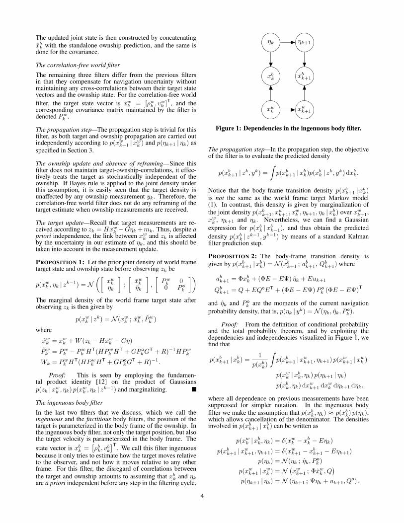
Figure 1: Dependencies in the ingenuous body filter.

The propagation step—In the propagation step, the objectiveof the filter is to evaluate the predicted density

p(xbk+1 | zk, yk) =

∫p(xbk+1 |xbk)p(xbk | zk, yk) dxbk.

Notice that the body-frame transition density p(xbk+1 |xbk)is not the same as the world frame target Markov model(1). In contrast, this density is given by marginalization ofthe joint density p(xbk+1, x

wk+1, x

wk , ηk+1, ηk |xbk) over xwk+1,

xwk , ηk+1 and ηk. Nevertheless, we can find a Gaussianexpression for p(xbk |xbk−1), and thus obtain the predicteddensity p(xbk | zk−1, yk−1) by means of a standard Kalmanfilter prediction step.

PROPOSITION 2: The body-frame transition density isgiven by p(xbk+1 |xbk) = N (xbk+1 ; abk+1, Q

bk+1) where

abk+1 = Φxbk + (ΦE − EΨ) ηk + Euk+1

Qbk+1 = Q+ EQoET + (ΦE − EΨ)P ok (ΦE − EΨ)

T

and ηk and P ok are the moments of the current navigation

probability density, that is, p(ηk | yk) = N (ηk, ηk, Pok ).

Proof: From the definition of conditional probabilityand the total probability theorem, and by exploiting thedependencies and independencies visualized in Figure 1, wefind that

p(xbk+1 |xbk) =1

p(xbk)

∫p(xbk+1 |xwk+1, ηk+1) p(xwk+1 |xwk )

p(xwk |xbk, ηk) p(ηk+1 | ηk)

p(xbk, ηk) dxwk+1 dxwk dηk+1 dηk.

where all dependence on previous measurements have beensuppressed for simpler notation. In the ingenuous bodyfilter we make the assumption that p(xbk, ηk) ≈ p(xbk) p(ηk),which allows cancellation of the denominator. The densitiesinvolved in p(xbk+1 |xbk) can be written as

p(xwk |xbk, ηk) = δ(xwk − xbk − Eηk)

p(xbk+1 |xwk+1, ηk+1) = δ(xwk+1 − xbk+1 − Eηk+1)

p(ηk) = N (ηk ; ηk, Pok )

p(xwk+1 |xwk ) = N(xwk+1 ; Φxwk , Q

)p(ηk+1 | ηk) = N (ηk+1 ; Ψηk + uk+1, Q

o) .

4

By stacking all the Gaussians together in one joint Gaussian,and integrating over xwk+1 and xwk , we get

p(xbk+1 |xbk) =

∫N

([xbk+1 + Eηk+1

ηk+1ηk

];

[Φ(xbk + Eηk)Ψηk + uk+1

ηk

],

[Q 0 00 Qo 00 0 P o

k

])dηk+1 dηk

In order to marginalize away ηk+1 and ηk we need to trans-form this into a Gaussian where xbk+1, ηk+1 and ηk only enteras a stacked vector in the random vector slot (and not in theexpectation slot). For this purpose we define the vectors

β =

[xbk+1ηk+1ηk

], ζ =

[Φxbkuk+1

ηk + uk+1

]and the matrices

A =

[I E −ΦE0 I −Ψ0 0 I

], Q =

[Q 0 00 Qo 00 0 P o

k

].

With these notations, the expression for p(xbk+1 |xbk) be-comes

p(xbk+1 |xbk) =

∫N(Aβ ; ζ, Q

)dηk+1 dηk

=

∫N(β ; A−1ζ, A−1Q(A−1)T

)dηk+1 dηk.

Inverting A is straightforward by means of standard resultsfor block matrices. The proposition follows from picking theupper 2 × 1-vector in A−1ζ and the upper left 2 × 2-matrixin A−1Q(A−1)T.

The ownship update and absence of reframing— When anownship measurement yk is received, the ownship state isupdated according to the standard Kalman filter correctionstep using the model described in Section 3. For the samereason as in the pure world filter, nothing happens to the targetestimate during this step.

The target update—For the ingenuous body filter, the targetstate xbk is updated by means of a standard Kalman filtercorrection step with the measurement model p(zk |xbk) =N (zk ; Hxbk, R). In this step, again due to the assumedindependence, nothing happens with the ownship estimate.

The factitious body filter

The factitious body filter is very similar to the ingenuous bodyfilter, but for this filter the velocity is parameterized in theworld frame. Thus, its state vector is xfk =

[ρbk, v

wk

]T.

The propagation step— It can be shown in a manner verysimilar to the proof of Proposition 2 that

p(xfk+1 |xfk) = N (xfk+1 ; afk+1, Q

fk+1)

where

afk+1 = Φxfk + (ΦT − TΨ) ηk + Tuk+1

Qfk+1 = Q+ TQoTT + (ΦT − TΨ)P ok (ΦT − TΨ)

T.

The ownship update and absence of reframing— For thefactitious body filter, the assumed independence betweenthe target state and the ownship state again implies that theownship update is carried out without affecting the target stateestimate.

The target update—Again, the target state is updated using alikelihood of the form p(zk |xfk) = N (zk ; Hxfk , R) withoutaffecting the ownship state.

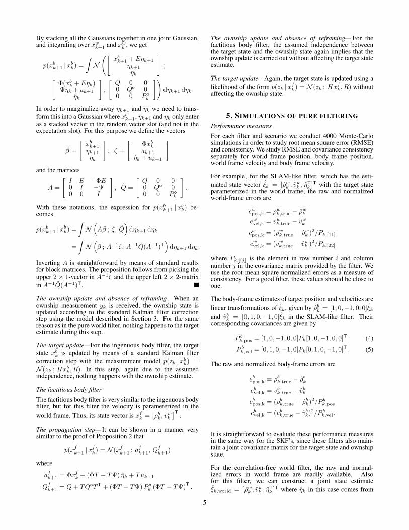
5. SIMULATIONS OF PURE FILTERINGPerformance measures

For each filter and scenario we conduct 4000 Monte-Carlosimulations in order to study root mean square error (RMSE)and consistency. We study RMSE and covariance consistencyseparately for world frame position, body frame position,world frame velocity and body frame velocity.

For example, for the SLAM-like filter, which has the esti-mated state vector ξk = [ρwk , v

wk , η

Tk ]T with the target state

parameterized in the world frame, the raw and normalizedworld-frame errors are

ewpos,k = ρwk,true − ρwkewvel,k = vwk,true − vwkcwpos,k = (ρwk,true − ρwk )2/Pk,[11]

cwvel,k = (vwk,true − vwk )2/Pk,[22]

where Pk,[ij] is the element in row number i and columnnumber j in the covariance matrix provided by the filter. Weuse the root mean square normalized errors as a measure ofconsistency. For a good filter, these values should be close toone.

The body-frame estimates of target position and velocities arelinear transformations of ξk, given by ρbk = [1, 0,−1, 0, 0]ξkand vbk = [0, 1, 0,−1, 0]ξk in the SLAM-like filter. Theircorresponding covariances are given by

P bk,pos = [1, 0,−1, 0, 0]Pk[1, 0,−1, 0, 0]T (4)

P bk,vel = [0, 1, 0,−1, 0]Pk[0, 1, 0,−1, 0]T. (5)

The raw and normalized body-frame errors are

ebpos,k = ρbk,true − ρbkebvel,k = vbk,true − vbkcbpos,k = (ρbk,true − ρbk)2/P bk,pos

cbvel,k = (vbk,true − vbk)2/P bk,vel.

It is straightforward to evaluate these performance measuresin the same way for the SKF’s, since these filters also main-tain a joint covariance matrix for the target state and ownshipstate.

For the correlation-free world filter, the raw and normal-ized errors in world frame are readily available. Alsofor this filter, we can construct a joint state estimateξk,world = [ρwk , v

wk , η

Tk ]T where ηk in this case comes from

5

Quantity Symbol/Units High noise Low noise

Ownship acceleration plant noise σ2o [m2/s5] (0.01)2 (0.01)2

Bias time constant 1/p [s] 1000 1000Mean square bias σ2

b [m/s2] (0.1)2 (0.1)2

GPS measurement noise Rη [m2] 102 102

Accelerometer white noise σ2w [m2/s3] (0.0002)2 (0.0002)2

Target measurement noise R [m2] (0.2)2 (0.01)2

Target plant noise σ2v [m2/s3] (1.0)2 (0.05)2

Acceleration sampling time [s] 0.01 0.01Target measurement sampling time [s] 2.5 2.5GPS sampling time [s] 1.0 1.0

Table 1: Simulation parameters

the standalone ownship navigation filter. The body frameestimates are then available as linear transformations ofξk,world according to ρbk = [1, 0,−1, 0, 0]ξk,world and vbk =

[0, 1, 0,−1, 0]ξk,world. To get the normalized errors we con-struct a joint covariance matrix, which in this case becomesblock-diagonal since no cross-correlations are maintained.The joint covariance is again transformed according to (5).We proceed in a similar manner for the correlation-free bodyfilters and for the basic world filter.

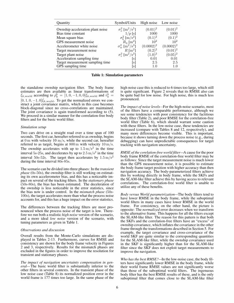
Simulation setup

Two cars drive on a straight road over a time span of 100seconds. The first car, hereafter referred to as ownship, beginsat 0 m with velocity 10 m/s, while the second car, hereafterreferred to as target, begins at 800 m with velocity 10 m/s.The ownship accelerates with up to 1.5 m/s2 in the timeinterval 5s-25s, and decelerates by up to 2.5 m/s2 in the timeinterval 50s-52s. The target then accelerates by 1.5 m/s2

during the time interval 80s-85s.

The scenario can be divided into three phases: In the transientphase (0s-50s), the ownship filter is still working on estimat-ing its own accelerometer bias, and this has a noticeable im-pact on several of the tracking filters. In the stationary phase(50s-80s), the bias has been estimated. The deceleration ofthe ownship is less noticeable in the error statistics, sincethe bias now is under control. In the mismatch phase (50s-100s), the target accelerates more than what the process noiseaccounts for, and this has a huge impact on the error statistics.

The differences between the tracking filters are most pro-nounced when the process noise of the target is low. There-fore we run both a realistic high noise version of the scenario,and a more ideal low noise version of the scenario, withtuning parameters as given in Table 1.

Observations and discussion

Overall results from the Monte-Carlo simulations are dis-played in Tables 2-13. Furthermore, curves for RMSE andconsistency are shown for the body frame velocity in Figures2 and 3, respectively. Results for the mismatch phases areexcluded in the figures in order to improve the resolution fortransient and stationary phases.

The impact of navigation uncertainty compensation in gen-eral—The basic world filter is substantially inferior to theother filters in several contexts. In the transient phase of thelow noise case (Table 8) its normalized position error in theworld frame is 177 times too large. In the same phase of the

high noise case this is reduced to 6 times too large, which stillis quite significant. Figure 2 reveals that its RMSE also canbe quite bad for low noise. For high noise, this is much lesspronounced.

The impact of noise levels—For the high-noise scenario, mostof the filters have a comparable performance, although wesee some tendencies with poor consistency for the factitiousbody filter (Table 2), and poor RMSE for the correlation-freeworld filter (Table 6), which should warrant some cautionwith these filters. In the low-noise case, these tendencies areincreased (compare with Tables 8 and 12, respectively), andmany more differences become visible. This is important,because it shows turning down the process noise (e.g., duringdebugging) can have unpredictable consequences for targettracking with navigation uncertainty.

RMSE of the corelation-free world filter—A cause for the poorbody frame RMSE of the correlation-free world filter may beas follows: Since the target measurement noise is much lowerthan the GPS measurement noise, it is possible to estimatethe body frame target position with higher accuracy than thennavigation accuracy. The body-parameterized filters achievethis by working directly in body frame, while the SKFs andthe SLAM-like filter achieve this by having access to relevantcorrelations. The correlation-free world filter is unable toutilize any of these benefits.

Body versus World parametrization—The body filters tend tohave lower RMSE in the body frame, while the suboptimalworld filters in many cases have lower RMSE in the worldframe. For consistency, on the other hand, the picture isopposite: The normalized error decreases when we transformto the alternative frame. This happens for all the filters exceptthe SLAM-like filter. The reason for this pattern is that boththe SKFs and the correlation-free filters have an “excess” ofownship covariance, which inflates the covariance in the otherframe through the transformations described in Section 5. Forexample, the target covariance and cross-covariance of theworld SKF are quite similar to the corresponding quantitiesfor the SLAM-like filter, while the ownship covariance usedin the SKF is significantly higher than for the SLAM-likefilter since the SKF does not exploit target measurements toimprove the navigation.

Who has the best RMSE?—In the low-noise case, the body fil-ters have significantly lower RMSE in the body frame, whiletheir world frame RMSE values are not significantly worsethan those of the suboptimal world filters. The ingenuousbody filter has the best RMSE results of these, and is the onlysuboptimal filter that comes close to the SLAM-like filter

6

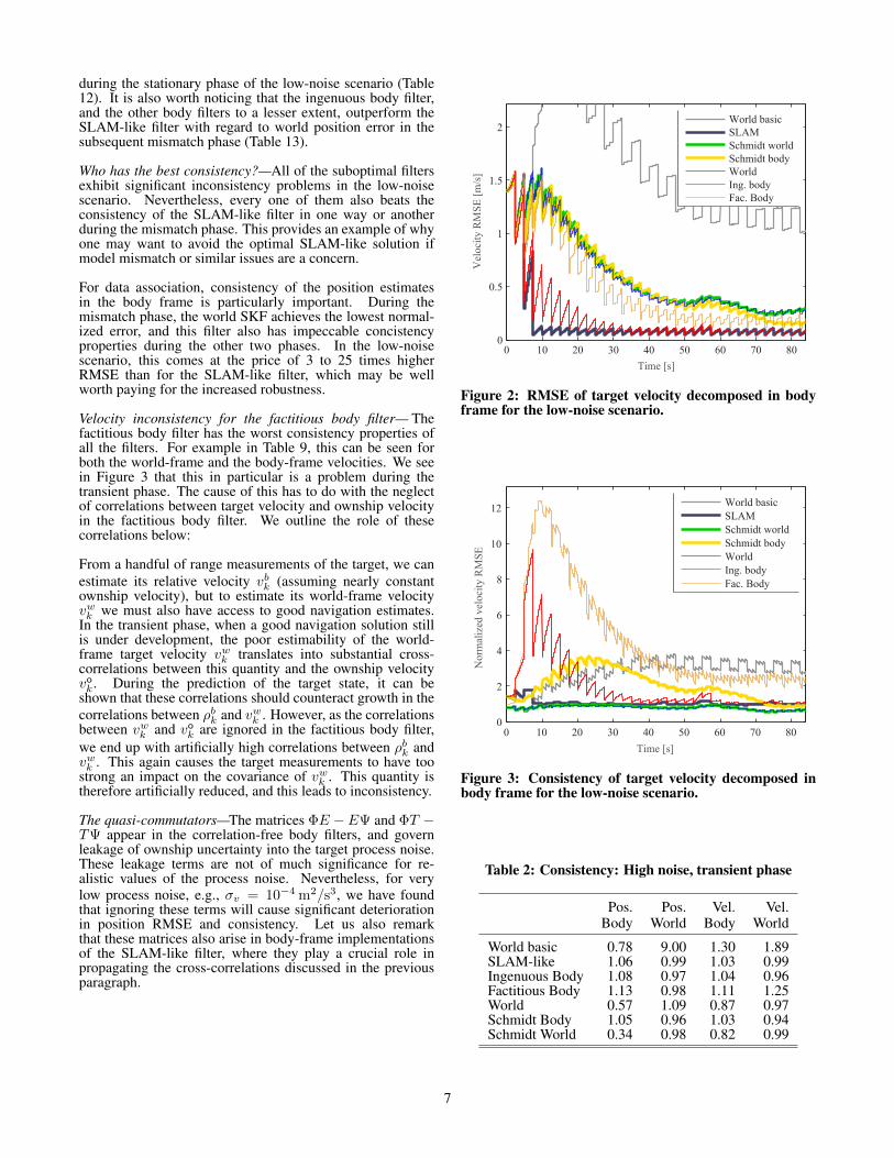
during the stationary phase of the low-noise scenario (Table12). It is also worth noticing that the ingenuous body filter,and the other body filters to a lesser extent, outperform theSLAM-like filter with regard to world position error in thesubsequent mismatch phase (Table 13).

Who has the best consistency?—All of the suboptimal filtersexhibit significant inconsistency problems in the low-noisescenario. Nevertheless, every one of them also beats theconsistency of the SLAM-like filter in one way or anotherduring the mismatch phase. This provides an example of whyone may want to avoid the optimal SLAM-like solution ifmodel mismatch or similar issues are a concern.

For data association, consistency of the position estimatesin the body frame is particularly important. During themismatch phase, the world SKF achieves the lowest normal-ized error, and this filter also has impeccable concistencyproperties during the other two phases. In the low-noisescenario, this comes at the price of 3 to 25 times higherRMSE than for the SLAM-like filter, which may be wellworth paying for the increased robustness.

Velocity inconsistency for the factitious body filter— Thefactitious body filter has the worst consistency properties ofall the filters. For example in Table 9, this can be seen forboth the world-frame and the body-frame velocities. We seein Figure 3 that this in particular is a problem during thetransient phase. The cause of this has to do with the neglectof correlations between target velocity and ownship velocityin the factitious body filter. We outline the role of thesecorrelations below:

From a handful of range measurements of the target, we canestimate its relative velocity vbk (assuming nearly constantownship velocity), but to estimate its world-frame velocityvwk we must also have access to good navigation estimates.In the transient phase, when a good navigation solution stillis under development, the poor estimability of the world-frame target velocity vwk translates into substantial cross-correlations between this quantity and the ownship velocityvok. During the prediction of the target state, it can beshown that these correlations should counteract growth in thecorrelations between ρbk and vwk . However, as the correlationsbetween vwk and vok are ignored in the factitious body filter,we end up with artificially high correlations between ρbk andvwk . This again causes the target measurements to have toostrong an impact on the covariance of vwk . This quantity istherefore artificially reduced, and this leads to inconsistency.

The quasi-commutators—The matrices ΦE −EΨ and ΦT −TΨ appear in the correlation-free body filters, and governleakage of ownship uncertainty into the target process noise.These leakage terms are not of much significance for re-alistic values of the process noise. Nevertheless, for verylow process noise, e.g., σv = 10−4 m2/s3, we have foundthat ignoring these terms will cause significant deteriorationin position RMSE and consistency. Let us also remarkthat these matrices also arise in body-frame implementationsof the SLAM-like filter, where they play a crucial role inpropagating the cross-correlations discussed in the previousparagraph.

Artificial text to push next section down.

0 10 20 30 40 50 60 70 800

0.5

1

1.5

2

Time [s]

Vel

ocity

RM

SE [m

/s]

RMSE − Body frame velocity

World basicSLAMSchmidt worldSchmidt bodyWorldIng. bodyFac. Body

Figure 2: RMSE of target velocity decomposed in bodyframe for the low-noise scenario.

0 10 20 30 40 50 60 70 800

2

4

6

8

10

12

Time [s]

Nor

mal

ized

vel

ocity

RM

SEConsistency − Body frame velocity

World basicSLAMSchmidt worldSchmidt bodyWorldIng. bodyFac. Body

Figure 3: Consistency of target velocity decomposed inbody frame for the low-noise scenario.

Table 2: Consistency: High noise, transient phase

Pos. Pos. Vel. Vel.Body World Body World

World basic 0.78 9.00 1.30 1.89SLAM-like 1.06 0.99 1.03 0.99Ingenuous Body 1.08 0.97 1.04 0.96Factitious Body 1.13 0.98 1.11 1.25World 0.57 1.09 0.87 0.97Schmidt Body 1.05 0.96 1.03 0.94Schmidt World 0.34 0.98 0.82 0.99

7

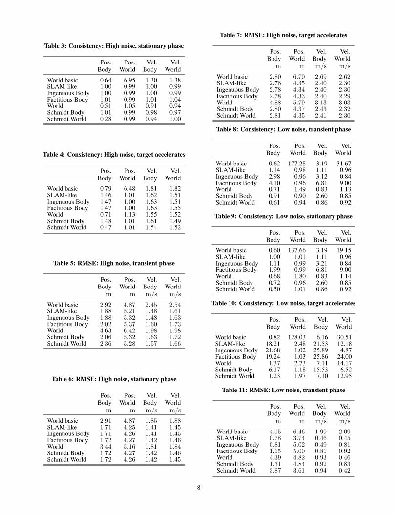
Table 3: Consistency: High noise, stationary phase



Table 4: Consistency: High noise, target accelerates



Table 5: RMSE: High noise, transient phase


m m m/s m/s


Table 6: RMSE: High noise, stationary phase


m m m/s m/s


Table 7: RMSE: High noise, target accelerates


m m m/s m/s


Table 8: Consistency: Low noise, transient phase



Table 9: Consistency: Low noise, stationary phase



Table 10: Consistency: Low noise, target accelerates



Table 11: RMSE: Low noise, transient phase


m m m/s m/s


8

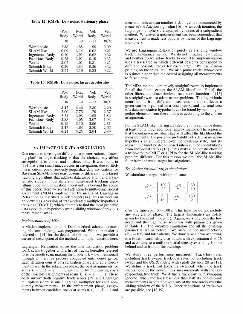
Table 12: RMSE: Low noise, stationary phase


m m m/s m/s


Table 13: RMSE: Low noise, target accelerates


m m m/s m/s


6. IMPACT ON DATA ASSOCIATIONOne reason to investigate different parameterizations of mov-ing platform target tracking is that the choices may affectsusceptibility to clutter and misdetections. It was found in[13] that even small inaccuracies in navigation, due to EKFlinearization, could seriously jeopardize data association forBayesian SLAM. There exist dozens of different multi-targettracking algorithms that address data association, and a sys-tematic study of how different multi-target tracking algo-rithms cope with navigation uncertainty is beyond the scopeof this paper. Here we restrict attention to multi-dimensionalassignment (MDA) implemented by means of LagrangianRelaxation as described in Deb’s paper [14]. This method canbe viewed as a version of track-oriented multiple hypothesistracking (TO-MHT) which attempts to find the most probabledata association hypothesis over a sliding window of previousmeasurement scans.

Implementation of MDA

A Matlab implementation of Deb’s method, adapted to mov-ing platform tracking, was programmed. While the reader isreferred to [14] for the details of the method, we provide acursorial description of the method and implementation here.

Lagrangian Relaxation solves the data association problemfor L scans (together with a list of tracks, hereafter referredto as the zeroth scan, making the problem L+1-dimensional)through an iterative process conducted until convergence.Each iteration consist of a relaxation phase and an enforce-ment phase. In the relaxation phase, the best assignments forscans L − 1, L − 2, . . . , 0 are found by minimizing costsof the possible assignments at scans L, L− 1, . . . , 1. Thesecosts involve both negative track scores [15] and Lagrangemultipliers (there is one Lagrange multiplier for each non-dummy measurement). In the enforcement phase, assign-ments between candidate tracks at scans 0, 1, . . . , L − 1 and

measurements at scan number 1, 2, . . . , L are constructed bymeans of the Auction algorithm [16]. After each iteration, theLagrange multipliers are updated by means of a subgradientmethod. Whenever a measurement has been contended, thatmeasurement is made less popular by means of the Lagrangemultipliers.

We use Lagrangian Relaxation purely as a sliding windowtrack maintenance method. We do not initialize new tracks,and neither do we allow tracks to die. The implementationuses a track tree in which different descents correspond todifferent possible tracks for each target. We use L-scanpruning on the track tree. We also prune tracks whose costis 6 times higher than the cost of assigning all measurementsto false alarms.

The MDA method is relatively straightforward to implementfor all the filters, except the SLAM-like filter. For all theother filters, the dimensionless track score function of [15]is straightforward to adapt to our problem. The logarithmiccontributions from different measurements and tracks at agiven can be organized in a cost matrix, and the total costof a data association hypothesis can be found by summing to-gether elements from these matrices according to the chosenassignment.

For the SLAM-like filtering architecture, this cannot be done,at least not without additional approximations. The reason isthat the unknown ownship state will affect the likelihood themeasurements. The posterior probability of a data associationhypothesis is an integral over the ownship state, and itslogarithm cannot be decomposed into a sum of contributionsfrom individual tracks [13]. This makes the construction ofa track-oriented MHT or a JPDA for the SLAM-like trackingproblem difficult. For this reason we omit the SLAM-likefilter from the multi-target investigations.

Test design for multi-target simulations

We simulate 4 targets with initial states

x(1)0 =

[10022

], x

(2)0 =

[5010

],

x(3)0 =

[016

], x

(4)0 =

[1502

],

over the time span 0 − 100 s. This time we do not includeany acceleration phase. The targets’ kinematics are solelygiven by the plant model (1). Again, we study both the lownoise and the high noise scenarios with parameters givenin Table 1. The ownship simulation and all the ownshipparameters are as before. We also include misdetections(PD = 0.8) and false alarms. We draw false alarms accordingto a Poisson cardinality distribution with expectation φ = 15and according to a uniform spatial density extending 1000mbehind and in front of the ownship.

We study three performance measures: Track-loss ratesincluding track swaps, track-loss rates not including trackswaps and the OSPA metric with cutoff distance 20 m [17].We define a track lost (possibly swapped) when the trackshares none of the non-dummy measurements with the cor-responding true track. We define a track lost, with swappingignored, when the track has less than half its non-dummymeasurements in common with any of the true tracks over thesliding window of the MDA. Other definitions of track-lossare possible, see [18,19].

9

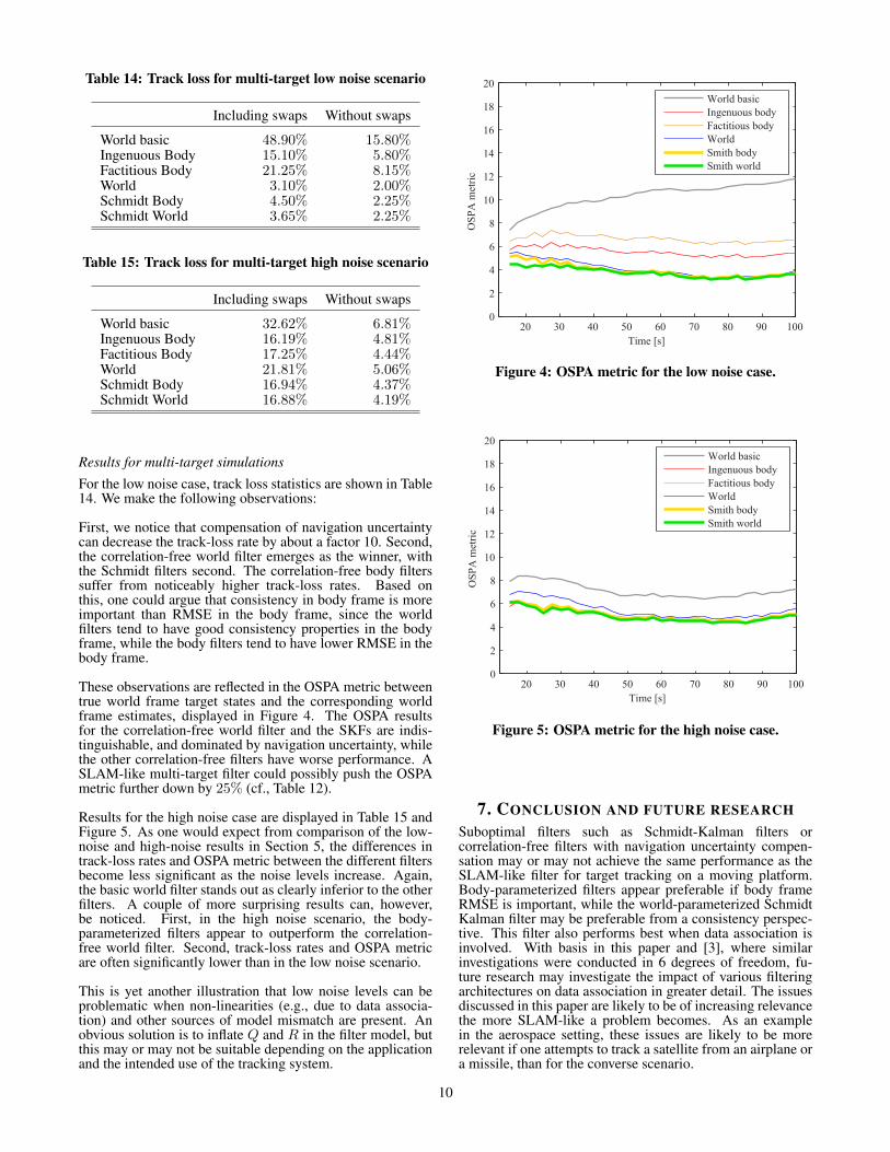
Table 14: Track loss for multi-target low noise scenario

Including swaps Without swaps

World basic 48.90% 15.80%Ingenuous Body 15.10% 5.80%Factitious Body 21.25% 8.15%World 3.10% 2.00%Schmidt Body 4.50% 2.25%Schmidt World 3.65% 2.25%

Table 15: Track loss for multi-target high noise scenario

Including swaps Without swaps

World basic 32.62% 6.81%Ingenuous Body 16.19% 4.81%Factitious Body 17.25% 4.44%World 21.81% 5.06%Schmidt Body 16.94% 4.37%Schmidt World 16.88% 4.19%

Results for multi-target simulations

For the low noise case, track loss statistics are shown in Table14. We make the following observations:

First, we notice that compensation of navigation uncertaintycan decrease the track-loss rate by about a factor 10. Second,the correlation-free world filter emerges as the winner, withthe Schmidt filters second. The correlation-free body filterssuffer from noticeably higher track-loss rates. Based onthis, one could argue that consistency in body frame is moreimportant than RMSE in the body frame, since the worldfilters tend to have good consistency properties in the bodyframe, while the body filters tend to have lower RMSE in thebody frame.

These observations are reflected in the OSPA metric betweentrue world frame target states and the corresponding worldframe estimates, displayed in Figure 4. The OSPA resultsfor the correlation-free world filter and the SKFs are indis-tinguishable, and dominated by navigation uncertainty, whilethe other correlation-free filters have worse performance. ASLAM-like multi-target filter could possibly push the OSPAmetric further down by 25% (cf., Table 12).

Results for the high noise case are displayed in Table 15 andFigure 5. As one would expect from comparison of the low-noise and high-noise results in Section 5, the differences intrack-loss rates and OSPA metric between the different filtersbecome less significant as the noise levels increase. Again,the basic world filter stands out as clearly inferior to the otherfilters. A couple of more surprising results can, however,be noticed. First, in the high noise scenario, the body-parameterized filters appear to outperform the correlation-free world filter. Second, track-loss rates and OSPA metricare often significantly lower than in the low noise scenario.

This is yet another illustration that low noise levels can beproblematic when non-linearities (e.g., due to data associa-tion) and other sources of model mismatch are present. Anobvious solution is to inflate Q and R in the filter model, butthis may or may not be suitable depending on the applicationand the intended use of the tracking system.

20 30 40 50 60 70 80 90 1000

2

4

6

8

10

12

14

16

18

20

Time [s]

OSP

A m

etric

World basicIngenuous bodyFactitious bodyWorldSmith bodySmith world

Figure 4: OSPA metric for the low noise case.

20 30 40 50 60 70 80 90 1000

2

4

6

8

10

12

14

16

18

20

Time [s]

OSP

A m

etric

World basicIngenuous bodyFactitious bodyWorldSmith bodySmith world

Figure 5: OSPA metric for the high noise case.

7. CONCLUSION AND FUTURE RESEARCHSuboptimal filters such as Schmidt-Kalman filters orcorrelation-free filters with navigation uncertainty compen-sation may or may not achieve the same performance as theSLAM-like filter for target tracking on a moving platform.Body-parameterized filters appear preferable if body frameRMSE is important, while the world-parameterized SchmidtKalman filter may be preferable from a consistency perspec-tive. This filter also performs best when data association isinvolved. With basis in this paper and [3], where similarinvestigations were conducted in 6 degrees of freedom, fu-ture research may investigate the impact of various filteringarchitectures on data association in greater detail. The issuesdiscussed in this paper are likely to be of increasing relevancethe more SLAM-like a problem becomes. As an examplein the aerospace setting, these issues are likely to be morerelevant if one attempts to track a satellite from an airplane ora missile, than for the converse scenario.

10

ACKNOWLEDGMENTSThis work was supported by the Research Council of Norwaythrough projects 223254 (Centre for Autonomous MarineOperations and Systems at NTNU) and 244116/O70 (SensorFusion and Collision Avoidance for Autonomous MarineVehicles).

REFERENCES[1] J. Sola, “Quaternion kinematics for the error-state KF,”

Mar. 2015. [Online]. Available: http://www.iri.upc.edu/people/jsola/JoanSola/objectes/notes/kinematics.pdf

[2] F. L. Markley, “Attitude error representations forkalman filtering,” Journal of Guidance, Control, andDynamics, vol. 26, no. 2, pp. 311 – 317, 2003.

[3] E. F. Wilthil and E. F. Brekke, “Compensation ofnavigation uncertainty for target tracking on a movingplatform,” in Proceedings of Fusion 2016, Heidelberg,Germany, Jul. 2016.

[4] C. S. Lee, D. E. Clark, and J. Salvi, “SLAM withdynamic targets via single-cluster PHD filtering,” IEEEJournal of Selected Topics in Signal Processing, vol. 7,no. 3, pp. 543 – 552, Jun. 2013.

[5] E. Brekke, B. Kalyan, and M. Chitre, “A novel formula-tion of the Bayes recursion for single-cluster filtering,”in Proceedings of IEEE Aerospace Conference, Big Sky,MT, USA, Mar. 2014.

[6] S. Julier and A. Gning, “Bernoulli filtering on a movingplatform,” in Proceedings of Fusion 2015, Washington,D.C., USA, July 2015, pp. 1511–1518.

[7] J. Sola, “Towards visual localization, mapping and mov-ing objects tracking by a mobile robot: a geometric andprobabilistic approach,” Ph.D. dissertation, l’InstitutNational Politechnique de Toulouse, 2007.

[8] Y. Bar-Shalom, “Mobile radar bias estimation usingunknown location targets,” in Proceedings of Fusion2000, Paris, France, 2000, pp. 3–6.

[9] R. Novoselov, S. Herman, S. Gadaleta, and A. Poore,“Mitigating the effects of residual biases with Schmidt-Kalman filtering,” in Proceedings of Fusion 2005,Philadelphia, PA, USA, July 2005.

[10] C. Yang, E. Blasch, and P. Douville, “Design ofSchmidt-Kalman filter for target tracking with naviga-tion errors,” in Proceedings of IEEE Aerospace Confer-ence, Big Sky, MT, USA, Mar. 2010, pp. 1–12.

[11] C. Van Loan, “Computing integrals involving the matrixexponential,” IEEE Transactions on Automatic Control,vol. 23, no. 3, pp. 395–404, 1978.

[12] M. Ulmke, O. Erdinc, and P. K. Willett, “Gaussianmixture cardinalized PHD filter for ground moving tar-get tracking,” in Proceedings of Fusion 2007, Quebec,Canada, July 2007.

[13] E. Brekke and M. Chitre, “A multi-hypothesis solutionto data association for the two-frame SLAM problem,”The International Journal of Robotics Research, vol. 34,no. 1, pp. 43–63, 2015.

[14] S. Deb, M. Yeddanapudi, K. Pattipati, and Y. Bar-Shalom, “A generalized S-D assignment algorithm formultisensor-multitarget state estimation,” IEEE Trans-actions on Aerospace and Electronic Systems, vol. 33,no. 2, pp. 523–538, Apr. 1997.

[15] Y. Bar-Shalom, S. S. Blackman, and R. J. Fitzgerald,“Dimensionless score function for multiple hypothesistracking,” IEEE Transactions on Aerospace and Elec-tronic Systems, vol. 43, no. 1, pp. 392–400, Jan. 2007.

[16] S. Blackman and R. Popoli, Design and Analysis ofModern Tracking Systems. Norwood, MA, USA:Artech House, 1999.

[17] D. Schuhmacher, B. T. Vo, and B.-N. Vo, “A consistentmetric for performance evaluation of multi-object fil-ters,” IEEE Transactions on Signal Processing, vol. 56,pp. 3447–3457, Aug. 2008.

[18] S. Coraluppi, D. Grimmett, and P. D. Theije, “Bench-mark evaluation of multistatic trackers,” in Proceedingsof Fusion 2006, Florence, Italy, July 2006.

[19] E. Brekke, O. Hallingstad, and J. Glattetre, “TheModified Riccati Equation for Amplitude-Aided TargetTracking in Heavy-Tailed Clutter,” IEEE Transactionson Aerospace and Electronic Systems, vol. 47, no. 4, pp.2874 – 2886, October 2011.

BIOGRAPHY[

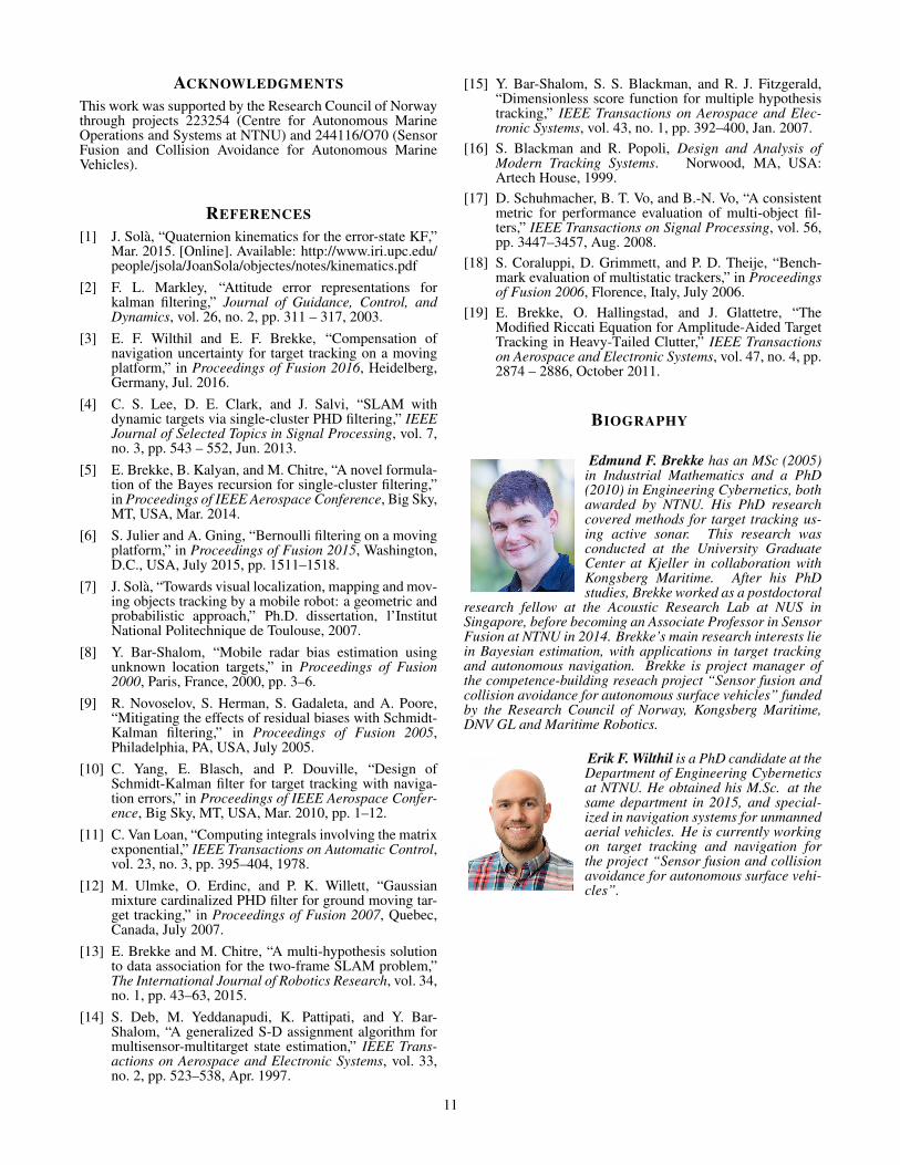
Edmund F. Brekke has an MSc (2005)in Industrial Mathematics and a PhD(2010) in Engineering Cybernetics, bothawarded by NTNU. His PhD researchcovered methods for target tracking us-ing active sonar. This research wasconducted at the University GraduateCenter at Kjeller in collaboration withKongsberg Maritime. After his PhDstudies, Brekke worked as a postdoctoral

research fellow at the Acoustic Research Lab at NUS inSingapore, before becoming an Associate Professor in SensorFusion at NTNU in 2014. Brekke’s main research interests liein Bayesian estimation, with applications in target trackingand autonomous navigation. Brekke is project manager ofthe competence-building reseach project “Sensor fusion andcollision avoidance for autonomous surface vehicles” fundedby the Research Council of Norway, Kongsberg Maritime,DNV GL and Maritime Robotics.

Erik F. Wilthil is a PhD candidate at theDepartment of Engineering Cyberneticsat NTNU. He obtained his M.Sc. at thesame department in 2015, and special-ized in navigation systems for unmannedaerial vehicles. He is currently workingon target tracking and navigation forthe project “Sensor fusion and collisionavoidance for autonomous surface vehi-cles”.

11

Suboptimal Kalman Filters for Target Tracking with Navigation ...

Documents