SUBMITTED VERSION - University of Adelaide

ACCEPTED VERSION

Yi Yang, Ching-Tai Ng, Andrei Kotousov Second-order harmonic generation of Lamb wave in prestressed plates Journal of Sound and Vibration, 2019; 460:114903-1-114903-12

© 2019 Elsevier Ltd. All rights reserved.

This manuscript version is made available under the CC-BY-NC-ND 4.0 license http://creativecommons.org/licenses/by-nc-nd/4.0/

Final publication at: http://dx.doi.org/10.1016/j.jsv.2019.114903

http://hdl.handle.net/2440/121631

PERMISSIONS

https://www.elsevier.com/about/policies/sharing

Accepted Manuscript

Authors can share their accepted manuscript:

24 Month Embargo

After the embargo period

via non-commercial hosting platforms such as their institutional repository via commercial sites with which Elsevier has an agreement

In all cases accepted manuscripts should:

link to the formal publication via its DOI bear a CC-BY-NC-ND license – this is easy to do if aggregated with other manuscripts, for example in a repository or other site, be shared in

alignment with our hosting policy not be added to or enhanced in any way to appear more like, or to substitute for, the published

journal article

17 November 2021

Second-order harmonic generation of Lamb wave in prestressed plates

Yi Yang1,*, Ching-Tai Ng1,†, Andrei Kotousov2,‡

1 School of Civil, Environmental & Mining Engineering, The University of Adelaide, SA 5005,

Australia

2 School of Mechanical Engineering, The University of Adelaide, SA 5005, Australia

Abstract

This paper investigates the second-order harmonics generation associated with propagation of

Lamb wave in pre-stressed plates. The second-order harmonic phenomena appear in a weakly

non-linear medium due to material and geometry nonlinearities. This study proposes finite

element (FE) models to incorporate stress constitutive equations formulated by Murgnahan’s

strain energy function. The model is used to take into account the stress effect on second-order

harmonic generation of Lamb wave propagation in weakly nonlinear media. The developed FE

model is first validated against two-dimensional (2D) analytical solutions. A three-dimensional

(3D) FE model is then developed and utilised to study more realistic problems, such as the rate

of accumulation of the non-linear parameter 𝛽′ at different wave propagation angles when the

plate is subjected to a bi-axial stress and the effect of the applied stresses on second-order

harmonic generation in a plate with a fatigue crack. The results demonstrate that the applied

stresses can notably change the value of 𝛽′ in different directions. The finding of this study can

gain physical insight into the physical phenomenon of stress effect on second-order harmonic

generation of Lamb wave. Thus, the current study opens an opportunity for the development

of a new non-destructive stress evaluation technique for plate- and shell-like structural

* Email: [email protected] † Corresponding author: A/Prof Ching Tai Ng ([email protected]) ‡ Email: [email protected]

components. Moreover, the new technique can be easily incorporated with existing guided

wave based-SHM systems and provide information regarding the change of the stress

conditions. Such additional information can significantly improve the structural life prognosis

and reduce risk of failures.

Keywords: Second-order harmonic; material nonlinearity; prestressed plate; finite element

simulation; stress effect

1. Introduction

The importance of Structural Health Monitoring (SHM) in engineering field is currently

undisputed, and benefits of SHM systems have been discussed in many papers [1]-[4]. SHM

systems based on ultrasonic guided waves, such as Rayleigh wave [5][6], Lamb wave [7],[8]

and torsional wave [9]-[10], have attracted attention over the past two decades [12]-[14], and

different damage detection techniques using linear guided wave were developed and deployed

across many industries [15]-[17]. One of the main objectives of the SHM systems is to provide

the information in a real time, which is required for structural life prognosis and maintenance

scheduling. However, the efficiency of the SHM systems as well as structural life prognosis is

significantly affected by changing environmental and operational conditions [18],[19], such as

the ambient temperature and applied loading on structures. Therefore, it is important to

incorporate the evaluation of these factors into the on-line monitoring systems in order to

improve the operation and maintenance procedures of high-value assets.

1.1. Acoustoelastic effect of Lamb waves

Most studies on the acoustoelastic of Lamb waves focused on the linear features, such as

change of the phase velocity with the magnitude of the applied stress. Gandhi et al. [20]

conducted a comprehensive analysis of the acoustoelastic effect associated with Lamb wave

propagation in plates subjected to bi-axial loading. However, this analysis only considered the

first-order of the infinitesimal strain tensor. In a recent study by Mohabuth et al. [21], a general

theory was developed, and the governing equations were derived for the propagation of small

amplitude waves in a pre-stressed plate using the theory of incremental deformations

superimposed on large deformations. They also extended the study to plates subjected to a bi-

axial stress [22] and investigate the large acoustoelastic effect of Lamb wave propagation in an

incompressible elastic plate. The correction to the phase velocity due to the applied stress was

obtained to the second order in pre-strain/stress [23]. The dispersion of the finite amplitude

Lamb waves was studied with a higher (or third)-order elastic theory by Packo et al. [24]. Yang

et al. [25] investigate the effect of axial stress on guided wave propagation using a semi-

analytical finite element method. They investigated the stress effect on phase and group

velocity of guided wave.

1.2. Nonlinear guided wave

There are many phenomena associated with non-linear guided waves, which can be utilised for

the damage and stress evaluation. These phenomena include the generation of higher-order

harmonics [26]-[28] and sidebands [29],[30]. According to the recent review of Jhang [31], the

non-linearity mainly arise from two sources, material non-linearity, and contact non-linearity

due to presence of contact-type defects or damage. The generation of higher-order harmonics

due to contact nonlinearity has been investigated experimentally for bulk waves [32], Rayleigh

waves [33]-[35] as well as for Lamb waves. A number of recent studies have also focused on

different types of damage, such as delamination [36]-[38], fatigue cracks [39]-[41], debonding

[42][43], and loosening bolted joints [44][45].

The material nonlinearity has been a subject of many theoretical and experimental

studies [26],[46]-[48]. According to the work of Pruell et al. [49] and Kim [50], plastic

deformations and fatigue damage can be a source of the material non-linearities, in addition to

the intrinsic non-linearity due to the inter-atomic and molecular forces. Therefore, it is possible

to evaluate the fatigue life and the accumulated plastic deformations based on the change of

the non-linear characteristics of ultrasonic waves. This possibility was recently demonstrated

experimentally by Hong et al. [51], who incorporated the intrinsic material non-linearity and

contact non-linearity associated with fatigue cracks and developed a method for fatigue damage

detection.

It has been demonstrated in several studies that the phase and group velocity matching,

and non-zero power flux are required to ensure that the higher-order harmonics grow with the

distance, and hence, it becomes detectible with piezoceramic transducer and other sensors.

Most of the studies considered the generation of the second-order harmonic associated with the

first order symmetric (S1) – second-order symmetric (S2) mode pairs of Lamb waves, which

satisfy the aforementioned matching conditions. Müller et al. [52] identified that there are five

mode types that satisfy the requirements for cumulative increase in second harmonic amplitude

through an analytical study. An experimental study of second harmonic generation was also

conducted by Matlack et al. [53]. The study investigated the efficiency of second harmonic

accumulation with propagation distances using both symmetric and anti-symmetric wave mode

pairs, which satisfy the aforementioned requirements. However, at the high frequency, there

are many wave modes, which makes it difficult to extract the non-linear parameter, such the

rate of accumulation of the second-order harmonic with the propagation distance. Moreover,

Lamb waves are normally excited using a finite frequency bandwidth. Because the S1 and S2

Lamb wave are highly dispersive at the matching condition frequencies, there is only a fraction

of the excitation power feeds the second-order harmonic, which make the accurate

measurements very challenging.

Wan et al. [48] found that the velocity change of the fundamental symmetric (S0) mode

of Lamb waves is quite small in low frequency region and the velocity matching conditions

can be satisfied approximately. Therefore, the generation and growth of the second-order

harmonic can also be observed over a certain propagation distance in low frequency ultrasonic

range. The propagation distance is closely related to the difference of the phase velocities

between the primary and second-order harmonic of Lamb waves. This study showed that the

data processing becomes much easier when only one Lamb wave mode exists. Moreover, the

excitation of S0 can be easily generated by using a common dual-transducer excitation method

[54].

1.3. Stress effect on higher harmonic generation of nonlinear guided wave

There were limited studies focused on investigating phenomena of higher-order harmonic

generation due to stress effect in the literature. In one-dimensional (1D) waveguide, Nucera

and Lanza di Scalea showed that the higher-order harmonic generation of guided wave can be

used to monitor load levels of multi-wire strands [55]. In their study, the higher-order

harmonics are generated due to the nonlinearity from inter-wire contact. In two-dimensional

(2D) waveguide, Pau and Lanza di Scalea [56] investigated the effect of the applied stress on

the generation of the second-order harmonic. They proposed an analytical model to investigate

the nonlinear guided wave propagation in prestressed plates.

The existing theoretical studies on the generation of the second-order harmonic are

typically very cumbersome and rest on adopting several crucial assumptions, such as plane

stress or plane strain conditions, which are difficult to reproduce in experiments. Therefore, the

outcomes of these studies cannot be readily adopted for practical purposes.

To address this problem, the current study in this paper develops a three-dimensional

(3D) FE model to gain fundamental understanding of the stress effect on the second-order

harmonic of Lamb waves under more realistic conditions i.e. conditions, which can be

relatively easy reproduced in the laboratory environment. The previous theoretical results are

utilised to validate this model. This provides the confidence in the outcomes of the more

realistic 3D analysis of the second-order harmonic generation.

The paper is structured as follows. Section 2 describes the constitutive equations based

on the Murgnahan’s strain energy function. Section 3 provides the details of the

implementation of the constitutive equations using VUMAT subroutine in ABAQUS software

package. In Section 4, the developed FE model is validated against analytical and numerical

results obtained under 2D assumptions. Section 5 presents a comprehensive 3D FE study of

the effect of the applied stresses on the rate of the accumulation of the second-order harmonic

at different wave propagation angles. Section 6 extends the current study to further consider

the prestressed plate with a fatigue crack. The main results and possible implementation of

these results to the stress evaluation are discussed in Section 7.

2. Constitutive Equations

The definition of position for material particle in the reference and current configuration

follows the definition of Mohabuth et al. [21][22], which are defined as 𝑿 and 𝒙, respectively.

The deformation gradient F is defined as

𝑭 = '𝒙'𝑿

(1)

The Green-Lagrange strain tensor is given by:

𝐄 = )*(𝐂 − 𝐈) (2)

where I is the identity tensor and C is the right Cauchy-Green deformation tensor, which is

defined as:

𝐂 = 𝐅1𝐅 = 𝐔𝟐 (3)

where U is the right stretch tensor.

The strain energy function according to Murnaghan [57] is written as:

W(𝐄) = )*(𝜆 + 2𝜇)𝑖)* − 2𝜇𝑖* +

):(𝑙 + 𝑚)𝑖)* − 2𝑚𝑖)𝑖* + 𝑛𝑖: (4)

where 𝜆 and 𝜇 are the lamé elastic constants; l, m and n are the third-order elastic constants or

Murgnahan’s constant. 𝑖) = tr(𝐄), 𝑖* =)*[𝑖)* − tr(𝐄)*], 𝑖: = det(𝐄), respectively, are strain

invariants. The partial derivatives of W with respect to E give the second Piola-Kirchhoff (PK2)

stress:

𝐓 = FG(𝐄)F𝐄

(5)

The relationship between Cauchy stress and PK2 stress is given by the following equation:

𝛔 = JJ)𝐅𝐓𝐅1 = JJ)𝐅 FG(𝐄)F𝐄

𝐅1 (6)

where J = det(𝐅).

3. Implementation the Constitutive Equations in Finite Element Simulation

In ABAQUS/Explicit, VUMAT subroutine is normally used to introduce the user-defined

constitutive behaviour of the material. VUMAT utilises the Cauchy stress tensor in Green-

Naghdi basis, which is given by

𝛔K = 𝐑1𝛔𝐑 (7)

where R is rotation tensor, and R is a proper orthogonal tensor, i.e., 𝐑J) = 𝐑1. The relationship

between F, U and R is given by

𝐅 = 𝐑𝐔 (8)

Using Equations (6) and (8), Equation (7) can be written as

𝛔K = JJ)𝐑1𝐅𝐓𝐅1𝐑 = JJ)𝐑1𝐑𝐔𝐓𝐔1𝐑1𝐑 = JJ)𝐔 FG(𝐄)F𝐄

𝐔1 (9)

Equation (9) provides the stress-strain relationship, which are programmed in the VUMAT

subroutine. The stress in VUMAT must be updated with in accordance to this equation at the

end (𝑡 + ∆𝑡) of an integration step and stored in stressNew(i) variable. These calculations are

based on the values of F and U given in the subroutine at the end of the previous step (𝑡).

4. Numerical Validation

This section presents the outcomes of a validation study of the VUMAT subroutine and FE

model as described in Section 2. It is validated against the theoretical results published by Wan

et al. [48]. A two-dimensional (2D) plane strain model is created in ABAQUS/Explicit and

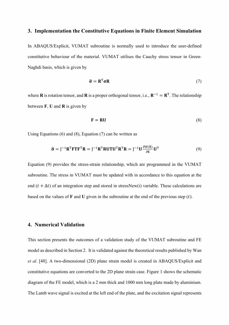
constitutive equations are converted to the 2D plane strain case. Figure 1 shows the schematic

diagram of the FE model, which is a 2 mm thick and 1000 mm long plate made by aluminium.

The Lamb wave signal is excited at the left end of the plate, and the excitation signal represents

a sinusoidal tone burst pulse modulated by a Hanning window. The excitation signal is

prescribed to the displacement at the nodal points. A fixed boundary condition is assigned to

the right end of the plate, which does not affect the calculations within a certain time window.

6061-T6 and 7075-T651 aluminium alloys are considered in the study and the material

properties of these alloys, including the third-order elastic constants, are given in Table 1.

Figure 1: Schematic diagram of 2D FE plate model in ABAQUS

Table 1. Material properties of 6061-T6 and 7075-T651 Material ρ (kg/m3) λ (GPa) μ (GPa) l (GPa) m (GPa) n (GPa) 6061-T6 2704 50.3 25.9 -281.5 -339 -416

7075-T651 2810 52.3 26.9 -252.2 -325 -351.2

In the FE analysis, the element size is selected to ensure that there are at least 20

elements per wavelength, so that the accuracy of the simulations is not compromised. There

are also eight elements in the thickness direction. Since the second-order harmonic generation

is of interest, the element size is selected based on the wavelength of the second-order harmonic

Lamb waves. The elements used in this study are 4-node bilinear plane strain quadrilateral

elements with reduced integration (CPE4R).

4.1. Second-order harmonic accumulation with the propagation distance

The maximum propagation distance within which the displacement amplitude of the second-

order harmonic increases [48]) is investigated. The excitation signals of 300 kHz and 400 kHz

corresponding to the fundamental symmetric mode (S0) of Lamb waves are excited at the left

end of the plate. The number of cycles of the wave signal is 18 and the excitation magnitude

of the displacement is set at 5 μm. For the 300 kHz excitation frequency, the measurement

points are taken at every 50 mm, and for 400 kHz excitation frequency the measurement points

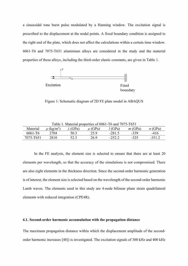
are at every 12.5 mm. Figure 2a show an example of the 300kHz wave signal measured at 200

mm away from the excitation area in the time-domain. Figure 2b show the signal in frequency-

domain. There are peak at excitation frequency 300 kHz and second-order harmonic frequency

600 kHz. The amplitudes of the second-order harmonic for the two fundamental excitation

frequencies, 600 kHz and 800 kHz, are extracted from the frequency-domain of the simulation

results and plotted in Figure 3. The results show that the maximum propagation distance of the

second-order harmonic Lamb wave at 600 kHz kHz and 800 kHz are 200 mm and 62.5 mm

respectively, and the corresponding theoretical values are 220.02 mm and 69.51 mm,

respectively [48].

Figure 2: a) Time- and b) frequency- domain of strain in x direction calculated at 200 mm

from the excitation location with 300kHz excitation signal

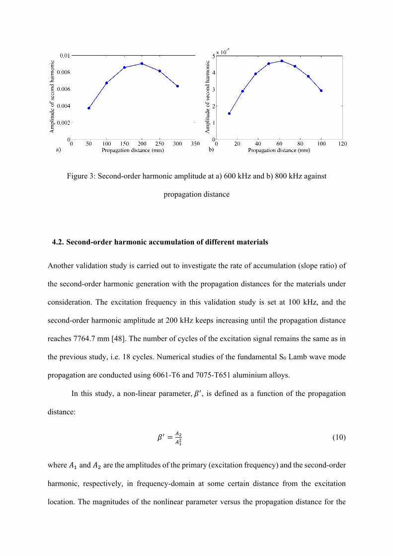
Figure 3: Second-order harmonic amplitude at a) 600 kHz and b) 800 kHz against

propagation distance

4.2. Second-order harmonic accumulation of different materials

Another validation study is carried out to investigate the rate of accumulation (slope ratio) of

the second-order harmonic generation with the propagation distances for the materials under

consideration. The excitation frequency in this validation study is set at 100 kHz, and the

second-order harmonic amplitude at 200 kHz keeps increasing until the propagation distance

reaches 7764.7 mm [48]. The number of cycles of the excitation signal remains the same as in

the previous study, i.e. 18 cycles. Numerical studies of the fundamental S0 Lamb wave mode

propagation are conducted using 6061-T6 and 7075-T651 aluminium alloys.

In this study, a non-linear parameter,𝛽O, is defined as a function of the propagation

distance:

𝛽O = PQPRQ

(10)

where 𝐴) and 𝐴* are the amplitudes of the primary (excitation frequency) and the second-order

harmonic, respectively, in frequency-domain at some certain distance from the excitation

location. The magnitudes of the nonlinear parameter versus the propagation distance for the

two cases of material properties specified in Table 1 are shown in Figure 4. The third-order

constants, 𝑙, 𝑚 and 𝑛, of 6061-T6 aluminium alloy are larger than those of 7075-T651. The

larger values of the third-order constants lead to larger values of the non-linear parameter and

a higher rate of the accumulation of the amplitude of the non-linear parameter with the

propagation distance. The slope of for the curve for 6061-T6 material properties is 0.00228

(mm-1), while for the 7075-T651 alloy the slope is 0.00205 (mm-1). As a result, the ratio

between these two slopes is around 1.11, compared to the theoretical value of 1.12 [48]. The

results show that there is good agreement between the theoretical and numerical result for all

validation studies.

Figure 4: Relative nonlinear parameter with propagation distance

5. Three-dimensional finite element study of prestressed plate

The 3D FE study is conducted for a 500 mm ´ 500 mm ´ 2mm plate. By taking advantage of

the symmetry of the problem, only a quarter of the plate is modelled using symmetry boundary

and the schematic diagram is shown in Figure 5. The material properties are those of 6061-T6

aluminium alloy. The S0 Lamb wave is excited at the corner of the model by applying 5 μm

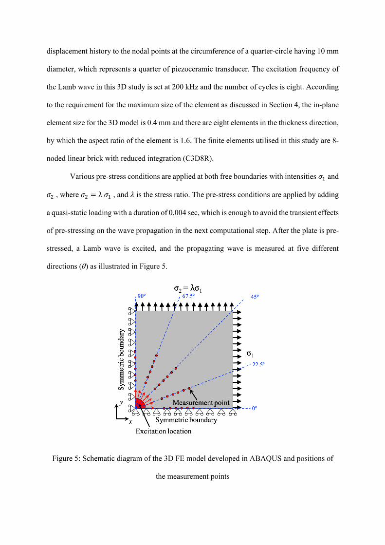
displacement history to the nodal points at the circumference of a quarter-circle having 10 mm

diameter, which represents a quarter of piezoceramic transducer. The excitation frequency of

the Lamb wave in this 3D study is set at 200 kHz and the number of cycles is eight. According

to the requirement for the maximum size of the element as discussed in Section 4, the in-plane

element size for the 3D model is 0.4 mm and there are eight elements in the thickness direction,

by which the aspect ratio of the element is 1.6. The finite elements utilised in this study are 8-

noded linear brick with reduced integration (C3D8R).

Various pre-stress conditions are applied at both free boundaries with intensities 𝜎) and

𝜎* , where 𝜎* = λ𝜎) , and 𝜆 is the stress ratio. The pre-stress conditions are applied by adding

a quasi-static loading with a duration of 0.004 sec, which is enough to avoid the transient effects

of pre-stressing on the wave propagation in the next computational step. After the plate is pre-

stressed, a Lamb wave is excited, and the propagating wave is measured at five different

directions (θ) as illustrated in Figure 5.

Figure 5: Schematic diagram of the 3D FE model developed in ABAQUS and positions of

the measurement points

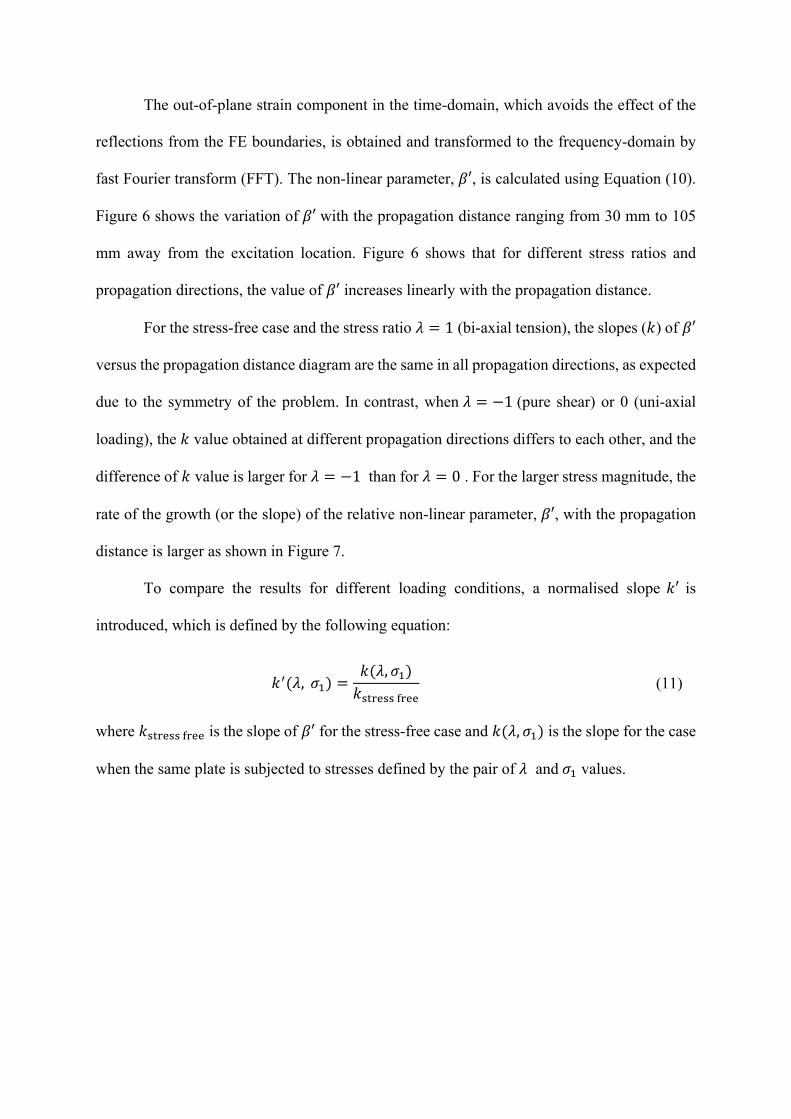
The out-of-plane strain component in the time-domain, which avoids the effect of the

reflections from the FE boundaries, is obtained and transformed to the frequency-domain by

fast Fourier transform (FFT). The non-linear parameter, 𝛽′, is calculated using Equation (10).

Figure 6 shows the variation of 𝛽′ with the propagation distance ranging from 30 mm to 105

mm away from the excitation location. Figure 6 shows that for different stress ratios and

propagation directions, the value of 𝛽′ increases linearly with the propagation distance.

For the stress-free case and the stress ratio 𝜆 = 1 (bi-axial tension), the slopes (𝑘) of 𝛽′

versus the propagation distance diagram are the same in all propagation directions, as expected

due to the symmetry of the problem. In contrast, when 𝜆 = −1 (pure shear) or 0 (uni-axial

loading), the 𝑘 value obtained at different propagation directions differs to each other, and the

difference of 𝑘 value is larger for 𝜆 = −1 than for 𝜆 = 0 . For the larger stress magnitude, the

rate of the growth (or the slope) of the relative non-linear parameter, 𝛽′, with the propagation

distance is larger as shown in Figure 7.

To compare the results for different loading conditions, a normalised slope 𝑘′ is

introduced, which is defined by the following equation:

𝑘O(𝜆, 𝜎)) =𝑘(𝜆, 𝜎))𝑘Z[\]ZZ^\]]

(11)

where 𝑘Z[\]ZZ^\]] is the slope of 𝛽′ for the stress-free case and 𝑘(𝜆, 𝜎)) is the slope for the case

when the same plate is subjected to stresses defined by the pair of 𝜆 and𝜎) values.

Figure 6: Relative nonlinear parameter for cases with a) stress free; b) σ1 = 100MPa, λ = 1; c)

σ1 = 100MPa, λ = -1; d) σ1 = 100MPa, λ = 0; and e) σ1 = -100MPa, λ = 1 condition

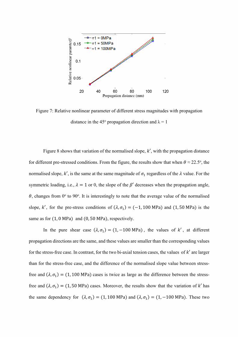
Figure 7: Relative nonlinear parameter of different stress magnitudes with propagation

distance in the 45o propagation direction and λ = 1

Figure 8 shows that variation of the normalised slope, 𝑘′, with the propagation distance

for different pre-stressed conditions. From the figure, the results show that when 𝜃 ≈ 22.5o, the

normalised slope, 𝑘′, is the same at the same magnitude of 𝜎) regardless of the 𝜆 value. For the

symmetric loading, i.e., 𝜆 = 1 or 0, the slope of the 𝛽′ decreases when the propagation angle,

𝜃, changes from 0o to 90o. It is interestingly to note that the average value of the normalised

slope, 𝑘′ , for the pre-stress conditions of (𝜆, 𝜎)) = (−1, 100MPa) and (1, 50MPa) is the

same as for (1, 0MPa) and (0, 50MPa), respectively.

In the pure shear case (𝜆, 𝜎)) = (1,−100MPa) , the values of 𝑘′ , at different

propagation directions are the same, and these values are smaller than the corresponding values

for the stress-free case. In contrast, for the two bi-axial tension cases, the values of 𝑘′ are larger

than for the stress-free case, and the difference of the normalised slope value between stress-

free and (𝜆, 𝜎)) = (1, 100MPa) cases is twice as large as the difference between the stress-

free and (𝜆, 𝜎)) = (1, 50MPa) cases. Moreover, the results show that the variation of 𝑘′ has

the same dependency for (𝜆, 𝜎)) = (1, 100MPa) and (𝜆, 𝜎)) = (1,−100MPa). These two

pre-stress conditions have the same magnitude of stress but the first represents the bi-axial

tension and the second represents a pure shear. The different patterns of the relative slope

variation indicate that, generally speaking, it is possible to evaluate the stress ratios and

principle stress directions in a pre-stressed plate based on the analysis of the angular variation

of the non-linearity parameter,𝛽′.

Figure 8: Variation of the normalised slope, 𝑘′ with the propagation distance for different pre-

stressed conditions.

6. Prestressed plate with a fatigue crack

As demonstrated in Section 5, the second-order harmonic generation could be affected by the

applied stresses on structures. The tensile stress could open an initially closed fatigue crack and

change the contact behaviour of the crack surface, as a consequence, the second-order harmonic

generation due to contact nonlinearity could be altered and this adds difficulty in detecting the

fatigue crack in the structures. In this section, the same 3D FE model used in Section 5 is

employed and a fatigue crack (Figure 9) is also modelled in this 3D FE model. The second-

0 10 20 30 40 50 60 70 80 900.9

0.95

1

1.05

1.1

Propagation direction (o)

Nor

mal

ised

slo

pe (k

')

Stress free(l,s1)=(1,100MPa)(l,s1)=(-1,100MPa)(l,s1)=(0,100MPa)(l,s1)=(0.5,100MPa)(l,s1)=(-0.5,100MPa)(l,s1)=(1,50Pa)(l,s1)=(0,-100MPa)(l,s1)=(1,-100MPa)

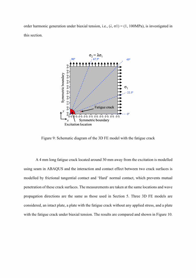
order harmonic generation under biaxial tension, i.e., (λ, σ1) = (1, 100MPa), is investigated in

this section.

Figure 9: Schematic diagram of the 3D FE model with the fatigue crack

A 4 mm long fatigue crack located around 30 mm away from the excitation is modelled

using seam in ABAQUS and the interaction and contact effect between two crack surfaces is

modelled by frictional tangential contact and ‘Hard’ normal contact, which prevents mutual

penetration of these crack surfaces. The measurements are taken at the same locations and wave

propagation directions are the same as those used in Section 5. Three 3D FE models are

considered, an intact plate, a plate with the fatigue crack without any applied stress, and a plate

with the fatigue crack under biaxial tension. The results are compared and shown in Figure 10.

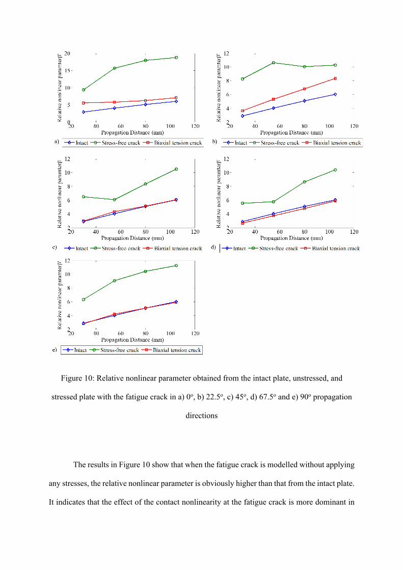
Figure 10: Relative nonlinear parameter obtained from the intact plate, unstressed, and

stressed plate with the fatigue crack in a) 0o, b) 22.5o, c) 45o, d) 67.5o and e) 90o propagation

directions

The results in Figure 10 show that when the fatigue crack is modelled without applying

any stresses, the relative nonlinear parameter is obviously higher than that from the intact plate.

It indicates that the effect of the contact nonlinearity at the fatigue crack is more dominant in

second-order harmonic generation than the intrinsic material nonlinearity. However, when the

biaxial tension is applied, the b’ drops to about the same level of that in the intact plate, except

for the cases of 0o and 22.5o propagation directions with the present of the fatigue crack around

these wave propagation angles. The phenomenon can be due to the fact that the fatigue crack

is opened by the tensile stress, which dramatically reduces the contact area between the crack

surfaces, and thus, it reduces the second-order harmonic generation due to the contact

nonlinearity. This parametric study demonstrates that the second-order harmonic generation

due to the fatigue crack can be overlooked if the plate is under tension, and hence, the fatigue

crack is opened by tensile stress. However, it should be noted that the 3D FE model does not

consider the plastic deformation around the fatigue crack, which will also generate extra

second-order harmonics [49]. Further study can be conducted to confirm the reliability of

second-order harmonic generation technique in detecting fatigue damage on a prestressed plate

with the consideration of the plastic deformation effect.

7. Conclusions

The study has investigated the effect of the pre-stressed conditions on the generation of the

second-order harmonic associated with propagation of low-frequency S0 Lamb wave using 3D

FE simulations. The material and geometric non-linearities have been modelled with the

classical Murnaghan’s strain energy function implemented in VUMAT subroutine of

ABAQUS software package and large-strain transient FE analysis, respectively. The non-linear

FE model has been extensively validated against 2D theoretical results. A good agreement

between the theoretical and numerical results has been achieved with the developed FE model.

The 3D FE model of the pre-stressed plate has been modelled and the change of the rate

of the accumulation of the second-order harmonic with the propagation distance has been

thoroughly investigated for different wave propagation angles (with respect to the principle

stresses) and pre-stress conditions. It has been found that different pre-stress conditions have

some unique features, which is potential to evaluate the stress state based on the analysis of

these non-linear features. This new possibility can be important for the development of future

on-line SHM systems.

The change of the non-linear parameter under the applied stress is of similar magnitude

as its variation in the case of fatigue damage accumulation. As it was demonstrated in the study

of Pruel et al. [49], the changes (increase) of the normalised non-linear parameter over the

fatigue life of an aluminium plate is roughly about 10%. Referring to Figure 8, the variation of

the non-linear parameter under stress can reach up to ±8%, which takes place in the pre-stress

case of (𝜆, 𝜎)) = (1,−100MPa) at 0o and 90o wave propagation direction. As a result, for

monitoring fatigue damage with the use of the second-order harmonic generation phenomenon

it will be necessary to consider the change of the applied or residual stresses in the structural

components.

Finally, the proposed 3D FE model has been used to study the stress effect on both

material nonlinearity and damage detection of the plate with the fatigue crack. The results have

shown that the second-order harmonic generation due to the contact nonlinearity can be

overlooked if the plate is under tension and the fatigue crack is opened by the tensile stress.

8. Acknowledgement

This work was supported by the Australian Research Council (ARC) under Grant Numbers

DP160102233. The support is greatly appreciated. The authors would like acknowledge Dr

Munawwar Mohabuth for the discussion of implementing the non-linear constitutive equations

in ABAQUS.

9. References

[1] Pan J, Zhang Z, Wu J, Ramakrishnan KR, Singh HK. A novel method of vibration

modes selection for improving accuracy of frequency-based damage detection.

Composites Part B: Engineering, 2019, 159:437-446.

[2] Zhang Z, Zhang C, Shankar K, Morozov EV, Singh HK, Ray T. Sensitivity analysis of

inverse algorithms for damage detection in composite. Composite Structures, 2017,

176:844-859.

[3] Zhang Z, Shankar K, Morozov EV, Tahtali M. Vibration-based delamination detection

in composite beams through frequency changes. Journal of Vibration and Control, 2016,

22:496-512.

[4] Bull L, Worden K, Manson G, Dervilis N. Active learning for semi-supervised

structural health monitoring. Journal of Sound and Vibration, 2018, 437:373-388.

[5] Ng CT, Mohseni H, Lam HF. Debonding detection in CFRP-retrofitted reinforced

concrete structures using nonlinear Rayleigh wave. Mechanical System and Signal

Processing, 2019, 125:245-256.

[6] Mohseni H, Ng CT. Rayleigh wave propagation and scattering characteristics at

debondings in fibre-reinforced polymer-retrofitted concrete structures. Structural

Health Monitoring, 2019, 18(1):303-317.

[7] Faisal Haider F, Bhuuyan MY, Poddar B, Lin B, Giurgiutiu V. Analytical and

experimental investigation of interaction of Lamb waves in stiffened aluminum plate

with a horizontal crack at the root of stiffener. Journal of Sound and Vibration, 2018,

431:212-225.

[8] Ng CT. On accuracy of analytical modeling of Lamb wave scattering at delaminations

in multilayered isotropic plates. International Journal of Structural Stability and

Dynamics, 2015, 15(8): 1540010.

[9] Leinov E, Lowe M.J.S., Cawley P. Investigation of guided wave propagation and

attenuation in pipe buried in sand. Journal of Sound and Vibration, 2015, 347: 96-114.

[10] Muggleton J.M., Kalkowski M, Gao Y, Rustighi E. A theoretical study of the

fundamental torsional wave in buried pipes for pipeline condition assessment and

monitoring, 2016, 374: 155-171.

[11] Yeung C, Ng CT. Time-domain spectral finite element method for analysis of torsional

guided waves scattering and mode conversion by cracks in pipes. Mechanical Systems

and Signal Processing, 2019, 128: 305-317.

[12] Park HW, Sohn H, Law KH, Farrar CR. Time reversal active sensing for health

monitoring of a composite plate. Journal of Sound and Vibration, 2007, 302(1-2): 50-

66.

[13] He S, Ng CT. A probabilistic approach for quantitative identification of multiple

delaminations in laminated composite beams using guided wave. Engineering

Structures, 2016, 127: 602-614.

[14] Senyurek VY, Baghalian A, Tashakori S, McDaniel D, Tansel IN. Localization of

multiple defects using the compact phased array (CPA) method. Journal of Sound and

Vibration, 2018, 413: 383-394.

[15] Aryan P, Kotousov A, Ng CT, Cazzolato B. A baseline-free and non-contact method

for detection and imaging of structural damage using 3D laser vibrometry. Structural

Control and Health Monitoring, 2017, 24(4): e1894.

[16] Zhou C, Zhang C, Su Z, Yue X, Xiang J, Li G. Health monitoring of rail structures

using guided waves and three-dimensional diagnostic image. Structural Control and

Health Monitoring, 2017, 24: e1966.

[17] Hughes JM, Vidler J, Ng CT, Khanna A, Mohabuth M, Rose LRF, Kotousov A.

Comparative evaluation of in situ stress monitoring with Rayleigh waves. Structural

Health Monitoring, 2019, 18(1): 205-215.

[18] Marzani A, Salamone S. Numerical prediction and experimental verification of

temperature effect on plate waves generated and received by piezoceramic sensors,

Mechanical Systems Signal Processing, 2012, 30: 204-217.

[19] Aryan P, Kotousov A, Ng CT, Wildy S. Reconstruction of baseline time-trace under

changing environmental and operational conditions. Smart Materials and Structures,

2016, 25: 035018.

[20] Gandhi N, Michaels JE, Lee SJ. Acoustoelastic Lamb wave propagation in biaxially

stressed plates. The Journal of the Acoustical Society of America, 2012, 132(3): 1284-

1293.

[21] Mohabuth M, Kotousov A, Ng CT. Effect of uniaxial stress on the propagation of

higher-order Lamb wave modes. International Journal of Non-Linear Mechanics, 2016,

86, 104-111.

[22] Mohabuth M, Kotousov A, Ng CT, Rose LRF. Implication of changing loading

conditions on structural health monitoring utilizing guided wave. Smart Materials and

Structures, 2018, 27: 025003.

[23] Mohabuth M, Kotousov A, Ng CT. Large acoustoelastic effect for Lamb waves

propagating in an incompressible elastic plate. The Journal of the Acoustical Society of

America, 2019, 145(3): 1221-1229.

[24] Packo P, Uhl T, Staszewski WJ, Leamy MJ. Amplitude-dependent Lamb wave

dispersion in nonlinear plates. The Journal of the Acoustical Society of America, 2016,

140(2): 1319-1331.

[25] Yang Z., Wu Z., Zhang J., Liu K. Jiang Y., Zhou K. Acoustoelastic guided wave

propagation in axial stressed arbitrary cross-section. Smart Materials and Structures,

2019, 28(4): 045013.

[26] Deng M. Cumulative second-harmonic generation of Lamb-mode propagation in a solid

plate. Journal of Applied Physics, 1999, 85(6): 3051-3058.

[27] Kube CM, Arguelles AP. Ultrasonic harmonic generation from materials with up to

cubic nonlinearity. The Journal of the Acoustical Society of America, 2017, 142:

EL224-EL230.

[28] Soleimanpour R, Ng CT, Wang CH. Locating delaminations in laminated composite

beams using nonlinear guided waves. Engineering Structures, 2017, 131: 207-219.

[29] Klepka A, Staszewski WJ, Maio DD, Scarpa F. Impact damage detection in composite

chiral sandwich panels using nonlinear vibro-acoustic modulations. Smart Materials

and Structures, 2013, 22: 084011.

[30] Liu P, Sohn H. Development of nonlinear spectral correlation between ultrasonic

modulation components. NDT & E International, 2017, 91: 120-128.

[31] Jhang KY. Nonlinear ultrasonic techniques for non-destructive assessment of micro

damage in material: A review, International Journal of Precision Engineering and

Manufacturing, 2009, 10(1): 123-135.

[32] Ohara Y, Takahashi K, Ino Y, Yamanaka K, Tsuji T, Mihara T. High-selectivity

imaging of closed cracks in a coarse-grained stainless steel by nonlinear ultrasonic

phased array. NDT & E International, 2017, 91: 139-147.

[33] Yuan M, Zhang J, Song SJ, Kim HJ. Numerical simulation of Rayleigh wave interaction

with surface closed cracks under external pressure. Wave Motion, 2015, 57: 143-153.

[34] Mohseni H, Ng CT. Higher harmonic generation of Rayleigh wave at debondings in

FRP-retrofitted concrete structures. Smart Materials and Structures, 2018, 27: 105038.

[35] Mohabuth M, Khanna A, Hughes J, Vidier J, Kotousov A, Ng CT. On the determination

of the third-order elastic constants of homogeneous isotropic materials utilizing

Rayleigh waves. Ultrasonics, 2019, https://doi.org/10.1016/j.ultras.2019.02.006

[36] Yelve NP, Mitra M, Mujumdar PM. Detection of delamination in composite laminates

using Lamb wave based nonlinear method. Composite Structures, 159(1): 257-266.

[37] Soleimanpour R, Ng CT, Wang CH. Higher harmonic generation of guided waves at

delaminations in laminated composite beams. Structural Health Monitoring, 2017,

16(4): 400-417.

[38] Liu X, Bo L, Yang K, Liu Y, Zhao Y, Zhang J, Hu N, Deng M. Locating and imaging

contact delamination based on chaotic detection of nonlinear Lamb waves. Mechanical

Systems and Signal Processing, 2018, 109: 58-73.

[39] He S, Ng CT. Modelling and analysis of nonlinear guided waves interaction at a

breathing crack using time-domain spectral finite element method. Smart Materials and

Structures, 2017, 26: 085002.

[40] Shen Y, Wang J, Xu W. Nonlinear features of guided wave scattering from rivet hole

nucleated fatigue cracks considering the rough contact surface condition. Smart

Materials and Structures, 2018, 27: 105044.

[41] Yang Y, Ng CT, Kotousov A. Influence of crack opening and incident wave angle on

second harmonic generation of Lamb waves. Smart Materials and Structures, 2018, 27:

055013.

[42] Scarselli G, Ciampa F, Ginzburg D, Meo M. Non-destructive testing techniques based

on nonlinear methods for assessment of debonding in single lap joints. SPIE

Proceedings, 2015, 9437: 943706.

[43] Mandal DD, Banerjee S. Identification of breathing type disbonds in stiffened panel

using non-linear lamb waves and built-in circular PWT array. Mechanical Systems and

Signal Processing, 2019, 117: 33-51.

[44] Amerini F, Meo M. Structural health monitoring of bolted joints using linear and

nonlinear acoustic/ultrasound methods. Structural Health Monitoring, 2011, 10(6): 659-

672.

[45] Yang Y, Ng CT, Kotousov A. Bolted joint integrity monitoring with second harmonic

generated by guided waves. Structural Health Monitoring, 2019, 18(1):193-204.

[46] Kube CM, Turner JA. Acoustic nonlinearity parameters for transversely isotropic

polycrystalline materials. The Journal of the Acoustical Society of America, 2015, 137:

3272-3280.

[47] Chillara VC, Lissenden CJ. Review of nonlinear ultrasonic guided wave nondestructive

evaluation: theory, numerics, experiments. Optical Engineering, 2016, 55(1): 011002.

[48] Wan X, Tse PW, Xu GH, Tao TF, Zhang Q. Analytical and numerical studies of

approximate phase velocity matching based nonlinear S0 mode Lamb waves for the

detection of evenly distributed microstructural changes. Smart Materials and Structures,

2016, 25:045023.

[49] Pruell C, Kim JY, Qu J, Jacobs LJ. A nonlinear-guided wave technique for evaluating

plasticity-driven material damage in a metal plate. NDT & E International, 2009, 42:

199-203.

[50] Kim JY, Jacobs LJ, Qu J. Experimental characterization of fatigue damage in nickel-

base superalloy using nonlinear ultrasonic waves. Journal of Acoustical Society of

America, 2006, 120(3): 1266-1273.

[51] Hong M, Su Z, Wang Q, Cheng L, Qing X. Modelling nonlinearities of ultrasonic waves

for fatigue damage characterization: Theory, simulation, and experimental validation.

Ultrasonics, 2014, 54: 770-778.c

[52] Müller MF, Kim JY, Qu J, Jacobs LJ. Characteristics of second harmonic generation of

Lamb waves in nonlinear elastic plates. Journal of Acoustical Society of America, 2010,

127(4): 2141-2152

[53] Matlack KH, Kim JY, Jacobs LJ, Qu J. Experimental characterization of efficient

second harmonic generation of Lamb wave modes in a nonlinear elastic isotropic plate.

Journal of Applied Physics, 2011, 109(1): 014905

[54] Sohn H. Reference-free crack detection under varying temperature. KSCE Journal of

Civil Engineering, 2011, 15(8): 1395-1404.

[55] Nucera C, Lanza di Scalea F. Monitoring load levels in multi-wire strands by nonlinear

ultrasonic waves. Structural Health Monitoring, 2011, 10(6): 617-629.

[56] Pau A, Lanza di Scalea F. Nonlinear guided wave propagation in prestressed plates.

The Journal of the Acoustical Society of America, 2015, 137(3): 1529-1540.

[57] Murnaghan FD. Finite deformation of an elastic solid. American Journal of

Mathematics, 1937, 59(2): 235-260.