Subdivision-Based Multilevel Methods for Large Scale ...sangria/publications/sm02-107-green.pdf · Subdivision-Based Multilevel Methods for Large Scale Engineering Simulation of Thin

Subdivision-Based Multilevel Methods for Large ScaleEngineering Simulation of Thin Shells

Seth GreenMechanical EngineeringUniversity of WashingtonSeattle, WA 98105; USA

[email protected]

George TurkiyyahCivil Engineering

University of WashingtonSeattle, WA 98105; USA

[email protected]

Duane StortiMechanical EngineeringUniversity of WashingtonSeattle, WA 98105; USA

[email protected]

ABSTRACTThis paper presents a multilevel algorithm to accelerate thenumerical solution of thin shell finite element problems de-scribed by subdivision surfaces. Subdivision surfaces havebecome a widely used geometric representation for generalcurved three dimensional boundary models and thin shellsas they provide a compact and robust framework for mod-eling 3D geometry. More recently, the shape functions usedin the subdivision surfaces framework have been proposedas candidates for use as finite element basis functions in theanalysis and simulation of the mechanical deformation ofthin shell structures. When coupled with standard solvers,however, such simulations do not scale well. Run time costsassociated with high-resolution simulations (105 degrees offreedom or more) become prohibitive.

The main contribution of the paper is to show that thesubdivision framework can be used for accelerating such sim-ulations. Specifically the subdivision matrix is used as theintergrid information transfer operator in a multilevel pre-conditioner. The method described in the paper allows thepractical simulation or a broad range of problems. Includedexamples show that the run time of the algorithm presentedscales nearly linearly in time with problem size.

Categories and Subject DescriptorsJ.2 [Physical Sciences and Engineering]: Engineering;J.6 [Computer-Aided Engineering]: Computer-aided de-sign (CAD)

General TermsAlgorithms, Design

KeywordsThin Shell, Numerical Algorithm, Multilevel, Multiresolu-tion, Multigrid, Subdivision Surface

Permission to make digital or hard copies of all or part of this work forpersonal or classroom use is granted without fee provided that copies arenot made or distributed for profit or commercial advantage and that copiesbear this notice and the full citation on the first page. To copy otherwise, torepublish, to post on servers or to redistribute to lists, requires prior specificpermission and/or a fee.SM’02,June 17-21, 2002, Saarbrucken, Germany.Copyright 2002 ACM 1-58113-506-8/02/0006 ...$5.00.

1. INTRODUCTIONSubdivision surfaces have become widely used geometric

representations of general curved three dimensional bound-ary models and thin shell objects. Their compactness, gener-ality and hierarchical structure have provided effective mech-anisms to support evaluating, querying, editing, fitting, andmanipulating 3D geometry in a robust and computationallyefficient manner.

More recently, the shape functions used in the subdivisionsurfaces framework have been proposed as candidates for useas finite element basis functions for the analysis and simula-tion of the mechanical deformation of thin shell structures.By construction, the subdivision shape functions provide thenecessary C1 continuity requirements (and H2 integrability)for representing the solution of the fourth-order equilibriumequations governing the behavior of thin shells. Subdivisionmodel descriptions also provide the rather elegant propertyof representing both the geometry and the physics of thedeformation using the same mathematical description.

Figure 1: Distributor Cap

Figure 1 shows a simulated deformation of engineeringmodel which is computationally expensive to compute. Whencoupled with standard solvers, such simulations do not scalewell. Given the fourth order nature of the governing equa-tions, the condition number of the underlying stiffness matri-ces grows as O( 1

h4 ), or O(n2), where h is a nominal elementlength scale and n is the number of degrees of freedom inthe discretized model. Using common preconditioned con-jugate gradient solvers, the number of iterations grows, atbest, linearly with problem size O(n), and run time growsas O(n2) even with the most efficient sparse representations.

In the context of high-resolution simulations involving largemeshes with n & 105 elements, the run time costs becomeprohibitive and present serious practical limits to the effec-tive use of simulation in engineering analysis.

In this paper, we describe an algorithm that exploits thehierarchical, multilevel structure of subdivision surfaces toaccelerate the convergence of solution strategies for thinshell simulations. We show that using the global subdivi-sion matrix for inter-level propagation of information leadsto solution methods in which the time to solution growsonly linearly with refinement for smooth models, and pro-vides significant acceleration for complex models with sharpfeatures. The strategies developed are not only useful onlarge scale meshes but are shown to be also advantageousfor relatively small problem sizes. The main contributionof the paper is to show that the subdivision framework canbe used not only for representing the geometry of the solidand the mechanics of the simulation, but also for precondi-tioning the numerical solution. This framework allows us toconstruct practical simulations that are effective on a broadrange of problems and problem sizes that are illustrated inthe paper.

The remainder of this paper is organized as follows. Webegin with a brief summary of the relevant aspects of theelements necessary to formulate the problem: subdivisionsurfaces, shell mechanics, and finite element discretizationin sections 2, 3 and 4 respectively. Section 5 includes a dis-cussion of multilevel solvers that leads to the presentationof our novel implementation of a multigrid-preconditionedconjugate gradient algorithm. Experimental results are pre-sented in section 6, and section 7 provides a discussion ofthe implementation aspects of our code, and the handlingof sharp features.

2. SUBDIVISION SURFACESSubdivision surfaces are increasingly used to represent

smooth shapes for engineering design. The subdivision frame-work provides a compact and efficient representation formodels with guaranteed smoothness properties, which areretained even if the model is deformed. Unlike traditionalspline approaches, subdivision representations do not re-quire complex cross-patch continuity constraints and canfreely model objects of arbitrary topology. Recently subdivi-sion surface representations have been shown to be effectivefor use in many stages of the modeling process includinggeneral modeling [10], interrogation [22], reconstruction [12,17], shape editing [25] dynamic simulation [14] and more.

Figure 2: Subdivision Refinement (Loop’s Scheme)

Subdivision surfaces are defined by an initial coarse meshknown as the control mesh. This initial mesh is refined re-

peatedly by rules defined by the chosen subdivision scheme.Repeated refinements lead to a hierarchy of increasingly re-fined models which approach the limit surface. Figure 2shows a model hierarchy in increasing stages of refinement.If the scheme is well formed, the refined meshes converge toa smooth surface. Most subdivision schemes are designedto produce a limit surface which smoothly approximates(but not necessarily interpolates) the initial control meshin shape.

2.1 Subdivision OperatorWe may refer to the vector of points representing the posi-

tions of the vertices of the mesh after j levels of subdivisionas pj , where j = 0 represents the control mesh itself. Thepositions of the vertices at level j are given by the formula

pj = Sjj−1p

j−1 (1)

where Sjj−1 represents the global subdivision operator, which

defines level j in terms of level j−1, and may be representedas a rectangular (and usually sparse) matrix. The entries ofSj

j−1 are defined by both the chosen subdivision scheme andthe topology (but not geometry) of the mesh at level j − 1.

2.2 Loop’s SchemeWhile many subdivision schemes have been proposed and

analyzed, we concentrate exclusively on Loop’s scheme fortriangular meshes. Loop’s scheme generalizes triangular boxsplines to meshes with arbitrary initial connectivity [13].This scheme is not interpolating but produces surfaces whichare known to be C2 continuous at all but a finite number ofextraordinary points; furthermore the scheme possesses thenecessary integrability [24] and refinement properties [1] tobe used as a basis in thin-shell finite element analysis. Ex-cellent reviews of Loop’s subdivision scheme may be foundin [21] and [7].

3. MECHANICS OF THIN SHELLSA thin shell is a three dimensional body in which one

geometric dimension, the thickness, is significantly smallerthan the other two. In the Kirchhoff-Love thin shell frame-work, the deformation of the body is fully described by thedeformation of its middle surface. The thin shell govern-ing equations may be derived from kinematic, constitutiveand equilibrium relations. More formal derivations may befound in [5] and [19]; here we present only the essentials ofthe argument.

3.1 KinematicsThe deformation of thin shells may be broken down into

two components:

1. A straining component that occurs in the surface ofthe shell measuring the stretching of the surface, andhence derivable from the first fundamental form of thesurface:

|ds|2 = aαβdθαdθβ (2)

where aαβ = aα · aβ is the covariant metric tensor ofthe surface defined by parameters θα and θβ .

2. A bending component measuring the change in curva-ture of the shell and hence derivable from the secondfundamental form of the surface

B = −bαβdθαdθβ (3)

where bαβ = a3·aβ,α. This requires that the curvaturebe evaluatable at all finite regions on the manifold

If the membrane (�) and bending strains (κ) are linearized,they may be written as a linear operator in terms of displace-ments (u). �

��

�=

�Ds

Db

�u = Du. (4)

3.2 Constitutive RelationsFor linear, isotropic materials the stresses and bending

moments may be written in terms of the membrane andbending strains as:�

�m

�=

E

1− ν2

"hC 0

0 h3

12C

#���

�= C

���

�(5)

where C is the standard plane stress constitutive matrix [5].

3.3 Equilibrium EquationsThe equilibrium equations relating externally applied forces

to the internal stresses (in-plane stretching/shearing forces,and bending moments) may be written through the princi-ple of virtual work, i.e. for all admissible displacements thefollowing relation holds:Z

S

(δ� : � + δκ : m) dS =

ZS

δu · f dS (6)

Substituting in the kinematics and constitutive relations ofthe previous sections, we arrive at the weak form of the thinshell governing equations:Z

S

δDu : CDu dS =

ZS

δu · f dS (7)

for all admissible δu. Given a set of applied forces f , we seekto determine the displacements u of the shell.

Kirchhoff-Love theory is the most widely used model forengineering analysis of thin shells. Other energy functionalshave been studied in the contexts of dynamic simulation andreconstruction of subdivision surfaces [17].

4. DISCRETIZATIONThe standard way of solving the governing equations is to

discretize them by representing the displacements u as lin-ear combinations of finite element basis functions (N) withcompact support [3]

u = NU. (8)

If each of the tensor quantities is “unwound” and writtenas a matrix Equation 7 becomes:

δUT

�ZS

(DN)T C(DN) dS

�U = δUT

�ZS

NT f dS

�∀δU.

(9)which can be described compactly as:

KU = F. (10)

where K is the stiffness matrix and F is the force vector.Cirak, et. al. [5, 4, 6] have successfully demonstrated the

utility of employing subdivision basis functions to representboth displacement fields and model geometry for thin shell

finite element simulations, which requires basis functionswith square integrable curvature tensors. Prior to the ad-vent of subdivision surface bases, maintaining the requiredderivative continuity across patch boundaries required highorder basis functions and constraints.

4.1 RefinementAs the number of elements (and therefore the number of

basis functions) used to represent the model is increased,more accurate solutions are obtained. Figure 3 shows anexample of the deflection of a curved surface modeled withincreasing refinement. An upwards concentrated load hasbeen placed near the center of the object in this simulation.When few elements are used, the local effect of the pointload cannot be adequately resolved. As the mesh is subdi-vided more elements are added, and the numerical solutionconverges to the exact solution. Rates of convergence ofvarious error estimates are described in [1] and [5].

Undeformed limit Deformed, level 0 Deformed, level 1surface

Deformed, level 2 Deformed, level 3 Deformed limitsurface

Figure 3: Refinement of Concentrated Load

Accurate solutions require a large number of elements,which is computationally expensive. A linear finite elementformulation with n degrees of freedom requires the inversionof a stiffness matrix K, of size n by n. Direct factorizationmethods require O(n3) operations to solve the system. Al-gorithms that take advantage of sparsity may run in O(n2)time [18]. Iterative methods may also be considered. As Kis positive definite, the conjugate gradient algorithm (CG)is a strong candidate for a solver.

The time to solution for iterative solvers is related tothe condition number of the system. The condition num-ber in turn is related to the element size distribution in themesh.The fourth-order nature of the equations governing theKirchhoff thin shell model result in the condition number ofthe system scaling as O(n2). Conjugate gradient is a robustand appropriate numerical technique, but for large prob-lems, performance O(n2) is unacceptable. Preconditioningthe system can lower the order and drastically reduce solu-tion effort; this is discussed in section 5.5.

5. MULTILEVEL SOLVERSMultilevel solvers can mitigate the cost associated with in-

creased accuracy by considering a hierarchy of refinementsof the model instead of only a single resolution. These so-lution schemes accelerate the convergence of numerical sim-

ulations by propagating solution values between finely dis-cretized representations of a model where accurate solutionsare obtained slowly, and coarsely discretized versions whereapproximate solutions may be obtained quickly. This pro-cess requires a hierarchical representation of multiple modelresolutions with an ability to transfer information betweenneighboring levels (both coarse-to-fine and fine-to-coarse,denoted “T” and “R”, respectively) as illustrated in Fig-ure 4. A well designed multilevel algorithm may achievesolution times of O(n).

R

T

R

T

Figure 4: An Example Multilevel Hierarchy

5.1 MultigridMultigrid (MG) methods are a family of multiresolution

methods that leverage the smoothing principle, which ap-plies to many numerical solution techniques for physical sys-tems [23]. In practice, error components with a high spatialfrequency are eliminated quickly, while those with a low spa-tial frequency decay more slowly.

Multigrid methods leverage this smoothing property bynoting that the troublesome low frequency error componentson a fine discretization may be well represented on a coarsermodel of the problem. Two main ingredients are required:smoothing and coarse grid correction. First, an iterativescheme is used to remove high frequency error components ofthe solution on a finely discretized version of the problem viasmoothing. Low frequency components of error may then beeliminated efficiently on a coarsely discretized model wherecomputation is less expensive. This process may be im-plemented recursively over many levels. Subdivision-basedfinite element meshes form a natural hierarchy that can beused for successive coarse grid corrections.

5.2 Multigrid AlgorithmMultigrid makes use of two operations for inter-grid trans-

fer of information. Prolongation (T ) and restriction (R)transfer from coarse to fine and fine to coarse levels respec-tively. These operators are discussed in detail in sections 5.3and 5.4. Pseudo code for the multigrid algorithm is shownbelow in Algorithm 1, adapted from [15], for solving the sys-tem Ku = f . For a system with an exact solution u and ancurrent approximate solution u, the residual is defined to ber = f −Ku, the error is e = u− u, and they are related asr = Ke. Were the error known, we could compute an exactsolution, but solving for the error explicitly is equivalent tosolving our original problem.

The process of repeatedly refining the error at a givenlevel is known as a W-Cycle. Each call to the multigridsolver that fully visits each level is known as a V-Cycle.Each smoothing step may require several internal iterations.The number of V and W-Cycles, and the number of internalsmoothing iterations, have a great effect on the performanceof the multigrid algorithm.

Algorithm 1 General Recursive Multigrid Algorithm

procedure: multigrid( l, u, t )

for each V-Cycle doif l = 0 then

u ⇐ K−10 f

elsefor each W-Cycle do

u ⇐ presmooth(l, u, b)r ⇐ f −Klur ⇐ Rlre ⇐ multigrid(l − 1,0, r)e = Tleu ⇐ u + eu ⇐ postsmooth(l, u, b)

end forend if

end for

5.3 ProlongationInformation defined on coarse grids must be prolongated

to finer levels via interpolation. Similarly, values defined onfine grids must be restricted to coarser levels, which resultsin a loss of information.

The choice of prolongation method is part of the designof any multigrid algorithm. We have chosen our prolonga-tion operator between levels j and j − 1 to be the globalsubdivision matrix Sj

j−1 itself. This choice retains the in-tuitive feature that a prolongated limit displacement fieldcorresponds exactly to the original limit displacement fieldof the coarser mesh. Thus we have now incorporated thesubdivision basis in three ways into our solution scheme: itdescribes the geometry, the displacement, and the connec-tion between levels in our multilevel hierarchy. The choice ofprolongation operator governs the choice of restriction oper-ator via work and energy considerations as discussed below.

5.4 RestrictionPhysical reasoning dictates that the work done by the ap-

plied forces be equivalent for each level of the hierarchy. Thisenergy requirement results in restriction operator being thetranspose of the prolongation operator. It is well known thatthis transpose relation holds for interpolating basis functionsgenerally used in finite element analysis [16] [8]. We showhere that this relation holds true for the choice of the subdi-vision operator for prolongation, which is not interpolatingin general. The work done by the generalized forces Fi mov-ing through generalized displacements Ui is given by:

W = UT F. (11)

We must emphasize the use of the term generalized dis-placements. Unlike interpolating bases which define thenodal displacements to be the actual displacement of a pointon the body at the nodal location, Loop subdivision ba-sis functions are non-interpolating and the displacements ofcontrol mesh vertices do not possess such a simple physicalinterpretation. Displacements on a finer level of the meshare given by:

Uj = Sjj−1U

j−1. (12)

Requiring equal work on two levels for arbitrary U using

the subdivision operator for restriction yields:�Uj�T

Fj =�Uj−1

�T

Fj−1 ∀Uj−1�Sj

j−1Uj−1�T

Fj =�Uj−1

�T

Fj−1 ∀Uj−1�Uj−1

�T �Sj

j−1

�T

Fj =�Uj−1

�T

Fj−1 ∀Uj−1

)�Sj

j−1

�T

Fj = Fj−1. (13)

This demonstrates that forces may be transferred from fineto coarse levels using the transpose of the subdivision opera-tor. Both the prolongation and restriction operators requireonly a single sparse matrix vector multiply and are com-putationally inexpensive. Qin has proposed an interleveltransfer operator outside of the multigrid context that usesthe psuedoinverse of the subdivision matrix [17].

5.5 Multigrid PreconditionedConjugate Gradient

The multigrid method provides a useful framework forsolving problems hierarchically, yet achieving optimal per-formance can be difficult. The algorithm relies on a handfulof tuning parameters, including the number of V and W cy-cles, and the number and kind of smoothing steps to applyper iteration. Proper tuning of these parameters remainsdifficult, and optimal performance of the multigrid by itselfcan be difficult to realize in practice.

Fortunately multigrid concepts can be easily integratedinto other strategies for solving linear systems. Multigridhas been shown to be significantly more effective when usedto precondition the conjugate gradient algorithm (CG). CGis specifically designed to take advantage of the positive def-initeness of the systems encountered in finite element simu-lations. Multigrid preconditioned conjugate gradient strate-gies (MGPCG) have been explored in mechanics and otherapplications [8, 15, 2].

MGPCG combines both multigrid and conjugate gradi-ent by using multigrid to compute the effect of a precon-ditioner. Multigrid may be used to solve the linear systemU = K−1F; this is exactly the computational form neededfor a preconditioner. A preconditioner need not be exactthough, and a full multigrid solution is expensive. Insteadof running multigrid to convergence, a few V cycle steps willsolve U ≈ K−1F. In practice a single V cycle is sufficientto effectively precondition the system. The matrix K−1 isnever explicitly formed, only its effect on vectors is needed.

6. RESULTSWe have run a variety of examples to verify and test the

performance of our method. These examples include a dis-tributor cap and fan housing (courtesy Hugues Hoppe), asquare flat plate, a hollow coiled tube, and a model withnon-trivial genus inspired by the ancient Egyptian “Ankh”symbol. Each of these models and their simulations areshown in figure 5 (the fan housing is shown separately infigure 10). The left column of figure 5 shows the coarsestlevel control meshes used to define the models, the middlecolumn shows sample loading conditions used for testing,and the right column shows the calculated deformed shape.The two rightmost columns are rendered after two levels ofsubdivision each.

Coarsest Limit Surface Deformed Level 2Control Mesh With Loads Limit Surface

Ankh

Distributor Cap

Coil

Plate

Figure 5: Models

For comparison, we have tested our own MGPCG solveragainst two other solution techniques, unpreconditioned con-jugate gradient and SuperLU [9]. Unpreconditioned CG wasselected to compare scaling behavior and contrast the effec-tiveness of using a multigrid preconditioner in our solver.SuperLU is an efficient general sparse direct matrix solverthat is freely available for academic use. Both MGPCG andCG were run until the solution residual was reduced by afactor of 105 (rn/r0 < 10−5).

Each level of subdivision increases the number of ele-ments and degrees of freedom of the model four-fold (moduloboundary effects). Because of this, setup times for the en-tire model hierarchy are not significantly larger than for thefinest level alone. Each model was simulated for a few dif-ferent levels of subdivision refinement. The MGPCG solveralways used the coarsest level for a base mesh and the num-ber of total levels in the hierarchy was equal to the givenlevel of subdivision. Logarithmic plots of solution time ver-sus the number of model degrees of freedom is shown forselected experiments to demonstrate efficiency and scalingbehavior; an algorithm of order O(np) will show a slope ofp on a log-log plot. A full listing of all results is given intable 1 at the end of this section. For the simplest models,

the very finest discretizations may be considered overkill;the experiments were performed to best show the scalingbehavior of the technique for very large problem sizes.

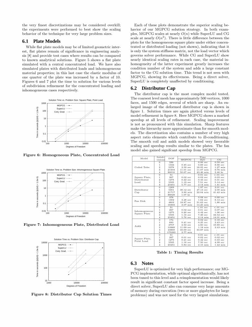
6.1 Plate ModelsWhile flat plate models may be of limited geometric inter-

est, flat plates remain of significance in engineering analy-sis [8] and provide test cases where results can be comparedto known analytical solutions. Figure 5 shows a flat platesimulated with a central concentrated load. We have alsosimulated plates with distributed loads and inhomogeneousmaterial properties; in this last case the elastic modulus ofone quarter of the plate was increased by a factor of 10.Figures 6 and 7 plot the time to solution for various levelsof subdivision refinement for the concentrated loading andinhomogeneous cases respectively.

0.01

0.1

1

10

100

1000

100 1000 10000 100000

Tim

e in

sec

onds

(|r

|/|r0

| < 1

.0e-

5)

Degrees of Freedom

Solution Time vs. Problem Size: Square Plate, Point Load

MGPCG

SuperLU

Conj. Grad.

Figure 6: Homogeneous Plate, Concentrated Load

0.01

0.1

1

10

100

1000

100 1000 10000 100000

Tim

e in

sec

onds

(|r

|/|r0

| < 1

.0e-

5)

Degrees of Freedom

Solution Time vs. Problem Size: Inhomogeneous Square Plate

MGPCG

SuperLU

Conj. Grad.

Figure 7: Inhomogeneous Plate, Distributed Load

10

100

1000

10000

1000 10000 100000

Tim

e in

sec

onds

(|r

|/|r0

| < 1

.0e-

5)

Degrees of Freedom

Solution Time vs. Problem Size: Distributor Cap

MGPCG

SuperLU

Conj. Grad.

Figure 8: Distributor Cap Solution Times

Each of these plots demonstrate the superior scaling be-havior of our MGPCG solution strategy. In both exam-ples, MGPCG scales at nearly O(n) while SuperLU and CGscale at nearly O(n2). There is little difference between theplots for the homogeneous square plate under either concen-trated or distributed loading (not shown), indicating that itis only the system stiffness matrix, not the load vector whichgoverns solver performance. While CG and SuperLU shownearly identical scaling rates in each case, the material in-homogeneity of the latter experiment greatly increases thecondition number of the system and adds a large constantfactor to the CG solution time. This trend is not seen withMGPCG, showing its effectiveness. Being a direct solver,SuperLU is completely unaffected by conditioning.

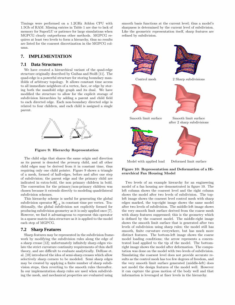
6.2 Distributor CapThe distributor cap is the most complex model tested.

The coarsest level mesh has approximately 500 vertices, 1000faces, and 1500 edges, several of which are sharp. An en-larged image of the deformed distributor cap is shown infigure 1. Solution times are again plotted versus levels ofmodel refinement in figure 8. Here MGPCG shows a markedspeedup at all levels of refinement. Scaling improvementis not as pronounced with this simulation. Sharp featuresmake the hierarchy more approximate than for smooth mod-els. The discretization also contains a number of very highaspect ratio elements which contribute to ill-conditioning.The smooth coil and ankh models showed very favorablescaling and speedup results similar to the plates. The fanmodel also gained signifcant speedup from MGPCG.

Model Subdi-visions DOF Time

MGPCG SLU CG

Coiled Tube

0 336 . 0.06 sec 0.59 sec1 1344 0.45 sec 0.69 sec 8.66 sec2 5376 2.59 sec 18.05 sec 1.27 min3 21504 11.01 sec 11.07 min 9.76 min4 86016 50.67 sec 43.46 min 2.46 hr

Square Plate,DistributedLoad

0 51 . 0.01 sec <.01 sec1 267 0.02 sec 0.02 sec 0.03 sec2 1275 0.22 sec 0.43 sec 0.31 sec3 5595 1.19 sec 7.51 sec 5.14 sec4 23451 5.77 sec 2.14 min 1.41 min

DistributorCap

0 1269 . 1.97 sec 3.01 sec1 5301 30.12 sec 47.13 sec 2.00 min2 21717 3.90 min 22.04 min 41.42 min3 88029 1.07 hr . .

Fan Disk

0 378 . 0.08 sec 0.68 sec1 1302 3.28 sec 1.62 sec 8.12 sec2 4803 18.87 sec 31.63 sec 1.86 min3 18393 3.07 min 14.25 min .

InhomogeneousSquare Plate

0 51 . <.01 sec <.01 sec1 267 0.02 sec 0.01 sec 0.07 sec2 1275 0.20 sec 0.42 sec 1.96 sec3 5595 1.16 sec 7.49 sec 44.52 sec4 23451 5.76 sec 2.14 min 14.01 min

Ankh

0 174 . 0.02 sec 0.18 sec1 693 0.41 sec 0.25 sec 2.43 sec2 2757 2.50 sec 4.60 sec 19.89 sec3 10989 11.69 sec 1.18 min 2.43 min4 43869 45.69 sec 33.87 min .5 175293 2.77 min . .

Square Plate,Point Load

0 51 . 0.01 sec <.01 sec1 267 0.01 sec 0.02 sec 0.02 sec2 1275 0.21 sec 0.42 sec 0.33 sec3 5595 1.16 sec 7.50 sec 4.99 sec4 23451 5.84 sec 2.15 min 1.42 min

Table 1: Timing Results

6.3 NotesSuperLU is optimized for very high performance; our MG-

PCG implementation, while optimal algorithmically, has notbeen tuned to this level and a reimplementation would likelyresult in significant constant factor speed increase. Being adirect solver, SuperLU also can consume very large amountsof memory during execution (two or more gigabytes for largeproblems) and was not used for the very largest simulations.

Timings were performed on a 1.2GHz Athlon CPU with1.5Gb of RAM. Missing entries in Table 1 are due to lack ofmemory for SuperLU or patience for large simulations whenMGPCG clearly outperforms other methods. MGPCG re-quires at least two levels to form a hierarchy, thus no resultsare listed for the coarsest discretization in the MGPCG col-umn.

7. IMPLEMENTATION

7.1 Data StructuresWe have created a hierarchical variant of the quad-edge

structure originally described by Guibas and Stolfi [11]. Thequad-edge is a powerful structure for storing boundary man-ifolds of arbitrary topology. It allows constant time accessto all immediate neighbors of a vertex, face, or edge by stor-ing both the manifold edge graph and its dual. We havemodified the structure to allow for the explicit storage ofsubdivision hierarchies by adding a parent and child fieldto each directed edge. Each non-boundary directed edge isrelated to four children, and each child is assigned a singleparent.

Figure 9: Hierarchy Representation

The child edge that shares the same origin and directionas its parent is denoted the primary child, and all otherchild edges may be derived from it in constant time, thusrequiring only one child pointer. Figure 9 shows a triangleof a mesh, formed of half-edges, before and after one stepof subdivision; the parent edge and the primary child areindicated in extra-bold, the non primary children in bold.The convention for the primary/non-primary children waschosen because it extends directly to modeling quadrilateralsubdivision schemes.

This hierarchy scheme is useful for generating the globalsubdivision operator Sj

j−1 in constant time per vertex. Tra-ditionally, the global subdivision not explicitly formed forproducing subdivision geometry as it is only applied once [7].However, we find it advantageous to represent this operatorin a sparse matrix data structure as it is applied to the modeleach step of MGPCG.

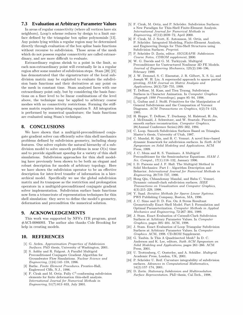
7.2 Sharp FeaturesSharp features may be represented in the subdivision frame-

work by modifying the subdivision rules along the edge ofa sharp crease [12]; unfortunately infinitely sharp edges vio-late the strict curvature continuity requirements of thin shelltheory, and are difficult to evaluate analytically. DeRose et.al. [10] introduced the idea of semi-sharp creases which allowselectively sharp corners to be modeled. Semi sharp edgesmay be created by applying a finite number of sharp subdi-vision steps, then reverting to the smooth rules thereafter.In our implementation sharp rules are used when subdivid-ing the mesh, and mechanical properties are evaluated using

smooth basis functions at the current level; thus a model’ssharpness is determined by the current level of subdivision.Like the geometric representation itself, sharp features arerefined by subdivision.

Control mesh 2 Sharp subdivisions

Smooth limit surface Smooth limit surfaceafter 2 sharp subdivisions

Model with applied load Deformed limit surface

Figure 10: Representation and Deformation of a Hi-erarchical Fan Housing Model

Two levels of an example hierarchy for an engineeringmodel of a fan housing are demonstrated in figure 10. Theleft column shows the coarsest level and the right columnshows the model after two levels of subdivision. The top-left image shows the coarsest level control mesh with sharpedges marked, the top-right image shows the same modelafter two levels of subdivision. The middle-left image showsthe very smooth limit surface derived from the coarse meshwith sharp features suppressed; this is the geometry whichis defined by the coarsest model. The middle-right imageshows the smooth limit surface that is generated after twolevels of subdivision using sharp rules; the model still hassmooth, finite curvature everywhere, but has much moredistinct features. The bottom-left image shows the coarsemodel loading conditions; the arrow represents a concen-trated load applied to the tip of the model. The bottom-right image shows the model after deformation. The compu-tation was done on the model with two levels of subdivision.Simulating the coarsest level does not provide accurate re-sults as the control mesh has too few degrees of freedom, andthe very smooth limit surface generated (middle-left) doesnot model the design features of the model well. Howeverit can capture the gross motion of the body well and thatinformation is leveraged at finer levels in the hierarchy.

7.3 Evaluation at Arbitrary Parameter ValuesIn areas of regular connectivity (where all vertices have six

neighbors), Loop’s scheme reduces by design to a limit sur-face defined by the triangular box spline polynomials [13].Any points lying within a regular region may be determineddirectly through evaluation of the box spline basis functionswithout recourse to subdivision. Those areas of the meshwhich do not possess regular connectivity are called extraor-dinary, and are more difficult to evaluate.

Extraordinary regions shrink to a point in the limit, soeach non-extraordinary point will eventually lie in a regularregion after some number of subdivision steps. Stam [20] [21]has demonstrated that the eigenstructure of the local sub-division matrix may be exploited to evaluate the subdivi-sion basis functions and their derivatives at any point onthe mesh in constant time. Stam analyzed faces with oneextraordinary point only, but by considering the basis func-tions on a finer level to be linear combinations of the levelabove, the technique may be applied to arbitrary coarsemeshes with no connectivity restrictions. Forming the stiff-ness matrix requires integrating equation 9. All integrationis performed by numerical quadrature; the basis functionsare evaluated using Stam’s technique.

8. CONCLUSIONSWe have shown that a multigrid-preconditioned conju-

gate gradient solver can efficiently solve thin shell mechanicsproblems defined by subdivision geometry, including sharpfeatures. Our solver exploits the natural hierarchy of a sub-division model to solve smooth problems in near O(n) timeand to provide significant speedup for a variety of thin shellsimulations. Subdivision approaches for thin shell model-ing have previously been shown to be both an elegant androbust description for models of arbitrary topology. Herewe have shown the subdivision operator to be an effectivedescription for inter-level transfer of information in a hier-archical model. Specifically we use the global subdivisionmatrix and its transpose as the restriction and prolongationoperators in a multigrid-preconditioned conjugate gradientsolver implementation. Subdivision surface basis functionsnow form a triumvirate of representation techniques for thinshell simulation: they serve to define the model’s geometry,deformation and precondition the numerical solution.

9. ACKNOWLEDGEMENTSThis work was supported by NFS’s ITR program, grant

#ACI-0086093. The author also thanks Cole Brooking forhelp in creating models.

10. REFERENCES[1] G. Arden. Approximation Properties of Subdivision

Surfaces. PhD thesis, University of Washington, 2001.[2] S. Ashby and R. Falgout. A Parallel Multigrid

Preconditioned Conjugate Gradient Algorithm forGroundwater Flow Simulations. Nuclear Science andEngineering, (124):145–159, 1996.

[3] Bathe. Finite Element Procedures. Prentice-Hall,Englewood Clffs, N.J., 1996.

[4] F. Cirak and M. Ortiz. Fully C1-conforming subdivisionelements for finite deformation thin-shell analysis.International Journal for Numerical Methods inEngineering, 51(7):813–833, July 2001.

[5] F. Cirak, M. Ortiz, and P. Schroder. Subdivision Surfaces:a New Paradigm for Thin-Shell Finite-Element Analysis.International Journal for Numerical Methods inEngineering, 47(12):2039–72, April 2000.

[6] F. Cirak, M. J. Scott, E. Antonsson, M. Ortiz, andP. Schroder. Integrated Modeling, Finite-Element Analysis,and Engineering Design for Thin-Shell Structures usingSubdivision Surfaces. Preprint.

[7] P. Schroder D. Zorin, editor. SIGGRAPH: SubdivisionCourse Notes, CDROM supplement, 2000.

[8] W. G. Davids and G. M. Turkiyyah. MultigridPreconditioner for Unstructured Nonlinear 3D FE Models.Journal of Engineering Mechanics, 125(2):186–196,February 1999.

[9] J. W. Demmel, S. C. Eisenstat, J. R. Gilbert, X. S. Li, andJoseph W. H. Liu. A supernodal approach to sparse partialpivoting. SIAM Journal on Matrix Analysis andApplications, 20(3):720–755, 1999.

[10] T. DeRose, M. Kass, and Tien Truong. SubdivisionSurfaces in Character Animation. In Computer Graphics(Siggraph 1998 Proceedings), pages 85–94, 1998.

[11] L. Guibas and J. Stolfi. Primitives for the Manipulation ofGeneral Subdivisions and the Compuation of VoronoiDiagrams. ACM Transactions on Graphics, 4(2):74–123,1985.

[12] H. Hoppe, T. DeRose, T. Duchamp, M. Halstead, H. Jin,J. McDonald, J. Schweitzer, and W. Stuetzle. Piecewisesmooth surface reconstruction. Computer Graphics,28(Annual Conference Series):295–302, 1994.

[13] C. Loop. Smooth Subdivision Surfaces Based on Triangles.Master’s thesis, University of Utah, 1987.

[14] C. Mandal, H. Qin, and B. C. Vemuri. A novel fem=baseddynamic framework for subdivision surfaces. In Sixth ACMSymposium on Solid Modeling and Applications. ACMPress, 1999.

[15] J. C. Meza and R. S. Tuminaro. A MultigridPreconditioner for the Semiconductor Equations. SIAM J.Sci. Comput., 17(1):118–132, January 1996.

[16] I. D. Parsons and J. F. Hall. The Multigrid Method inSolid Mechanics: Part I - Algorithm Description andBehavior. International Journal for Numerical Methods inEngineering, 29:719–737, 1990.

[17] Hong Qin, Chhandomay Mandal, and Baba C. Vemuri.Dynamic catmull-clark subdivision surfaces. IEEETransactions on Visualization and Computer Graphics,4(3):215–229, 1998.

[18] Y. Saad. Iterative Methods for Sparse Linear Systems.PWS Publishing Company, Boston, MA, 1996.

[19] J. C. Simo and D. D. Fox. On A Stress ResultantGeometrically Exact Shell Model. Part I: Formulation andOptimal Parameterization. Computer Methods in AppliedMechanics and Engineering, 72:267–304, 1989.

[20] J. Stam. Exact Evaluation of Catmull-Clark SubdivisionSurfaces at Arbitrary Parameter Values. In ComputerGraphics, pages 395–404. ACM, 1998.

[21] J. Stam. Exact Evaluation of Loop Triangular SubdivisionSurfaces at Arbitrary Parameter Values. In ComputerGraphics. ACM, 1998. CD-ROM Supplement.

[22] G. Taubin. Is This A Quadrisected Mesh? In D. C.Anderson and K. Lee, editors, Sixth ACM Symposium onSolid Modeling and Applications, pages 261–266. ACMPress, 2001.

[23] U. Trottenberg, C. Oosterlee, and A. Schuller. Multigrid.Academic Press, London, UK, 2001.

[24] P. Schroder U. Reif. Curvature integrability of subdivisionsurfaces. Advances in Computational Mathematics,14(2):157–174, 2001.

[25] D. Zorin. Stationary Subdivision and MultiresolutionSurface Representation. PhD thesis, Cal.Tech., 1998.