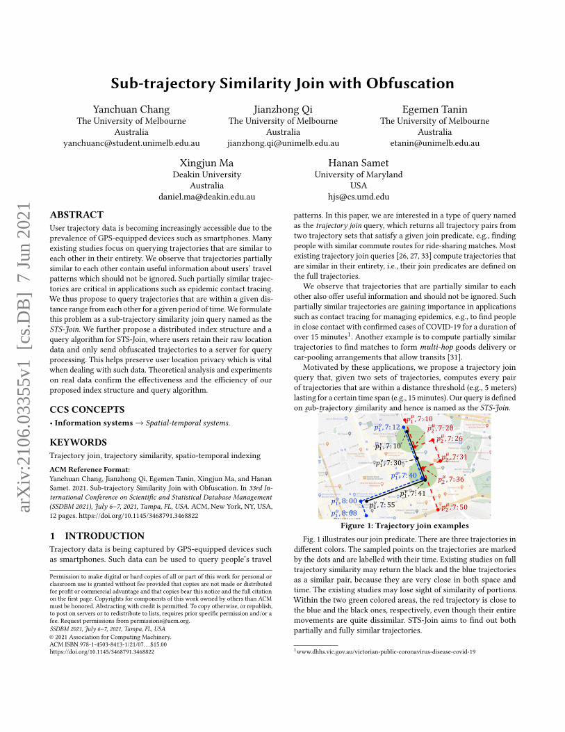
Sub-trajectory Similarity Join with Obfuscation - arXiv

Sub-trajectory Similarity Join with ObfuscationYanchuan Chang

The University of Melbourne

Australia

[email protected]

Jianzhong Qi

The University of Melbourne

Australia

[email protected]

Egemen Tanin

The University of Melbourne

Australia

[email protected]

Xingjun Ma

Deakin University

Australia

[email protected]

Hanan Samet

University of Maryland

USA

[email protected]

ABSTRACTUser trajectory data is becoming increasingly accessible due to the

prevalence of GPS-equipped devices such as smartphones. Many

existing studies focus on querying trajectories that are similar to

each other in their entirety. We observe that trajectories partially

similar to each other contain useful information about users’ travel

patterns which should not be ignored. Such partially similar trajec-

tories are critical in applications such as epidemic contact tracing.

We thus propose to query trajectories that are within a given dis-

tance range from each other for a given period of time.We formulate

this problem as a sub-trajectory similarity join query named as the

STS-Join. We further propose a distributed index structure and a

query algorithm for STS-Join, where users retain their raw location

data and only send obfuscated trajectories to a server for query

processing. This helps preserve user location privacy which is vital

when dealing with such data. Theoretical analysis and experiments

on real data confirm the effectiveness and the efficiency of our

proposed index structure and query algorithm.

CCS CONCEPTS• Information systems→ Spatial-temporal systems.

KEYWORDSTrajectory join, trajectory similarity, spatio-temporal indexing

ACM Reference Format:Yanchuan Chang, Jianzhong Qi, Egemen Tanin, Xingjun Ma, and Hanan

Samet. 2021. Sub-trajectory Similarity Join with Obfuscation. In 33rd In-ternational Conference on Scientific and Statistical Database Management(SSDBM 2021), July 6–7, 2021, Tampa, FL, USA. ACM, New York, NY, USA,

12 pages. https://doi.org/10.1145/3468791.3468822

1 INTRODUCTIONTrajectory data is being captured by GPS-equipped devices such

as smartphones. Such data can be used to query people’s travel

Permission to make digital or hard copies of all or part of this work for personal or

classroom use is granted without fee provided that copies are not made or distributed

for profit or commercial advantage and that copies bear this notice and the full citation

on the first page. Copyrights for components of this work owned by others than ACM

must be honored. Abstracting with credit is permitted. To copy otherwise, or republish,

to post on servers or to redistribute to lists, requires prior specific permission and/or a

fee. Request permissions from [email protected].

SSDBM 2021, July 6–7, 2021, Tampa, FL, USA© 2021 Association for Computing Machinery.

ACM ISBN 978-1-4503-8413-1/21/07. . . $15.00

https://doi.org/10.1145/3468791.3468822

patterns. In this paper, we are interested in a type of query named

as the trajectory join query, which returns all trajectory pairs from

two trajectory sets that satisfy a given join predicate, e.g., finding

people with similar commute routes for ride-sharing matches. Most

existing trajectory join queries [26, 27, 33] compute trajectories that

are similar in their entirety, i.e., their join predicates are defined on

the full trajectories.

We observe that trajectories that are partially similar to each

other also offer useful information and should not be ignored. Such

partially similar trajectories are gaining importance in applications

such as contact tracing for managing epidemics, e.g., to find people

in close contact with confirmed cases of COVID-19 for a duration of

over 15 minutes1. Another example is to compute partially similar

trajectories to find matches to form multi-hop goods delivery or

car-pooling arrangements that allow transits [31].

Motivated by these applications, we propose a trajectory join

query that, given two sets of trajectories, computes every pair

of trajectories that are within a distance threshold (e.g., 5 meters)

lasting for a certain time span (e.g., 15minutes). Our query is defined

on sub-trajectory similarity and hence is named as the STS-Join.!!* , 7: 10

!#* , 7: 20!#* , 7: 26

!#* , 7: 31

!#* , 7: 36

!#* , 7: 50

!!+ , 7: 12

!!+ , 8: 00!!+ , 8: 08

!!, , 7: 10

!!, , 7: 30

!!, , 7: 41!!, , 7: 55

!!+ , 7: 40

Figure 1: Trajectory join examples

Fig. 1 illustrates our join predicate. There are three trajectories in

different colors. The sampled points on the trajectories are marked

by the dots and are labelled with their time. Existing studies on full

trajectory similarity may return the black and the blue trajectories

as a similar pair, because they are very close in both space and

time. The existing studies may lose sight of similarity of portions.

Within the two green colored areas, the red trajectory is close to

the blue and the black ones, respectively, even though their entire

movements are quite dissimilar. STS-Join aims to find out both

partially and fully similar trajectories.

1www.dhhs.vic.gov.au/victorian-public-coronavirus-disease-covid-19

arX

iv:2

106.

0335

5v1

[cs

.DB

] 7

Jun

202

1

SSDBM 2021, July 6–7, 2021, Tampa, FL, USA Yanchuan Chang et al.

We assume a distributed (i.e., client-server) system architecture

to process STS-Join queries. Each client device (e.g., a user’s mobile

phone) stores a user’s own accurate trajectories, while the server

only stores a modified version of the trajectories for privacy consid-

erations. To showcase the feasibility of processing STS-Join queries

over modified trajectories, we consider trajectory obfuscation. A

user trajectory is obfuscated automatically where every sampled

point on the trajectory is shifted with a bounded-distance noise be-

fore the trajectory is sent to the server. All users’ obfuscated trajecto-

ries are thenmaintained on the server in a spatio-temporal index for

fast query retrieval. We note that there are limitations in using only

obfuscation for trajectory privacy protection, and more advanced

techniques exist in the literature such as geo-indistinguishability [4].

However, the core theme and contribution of our study is not topropose another privacy protection technique. Thus, we just use

obfuscation for its simplicity and leave more advanced privacy

protection techniques for future studies.

We propose a query algorithm for STS-Join based on a traversal

over our index structure. To take advantage of the characteristic that

segments on a trajectory are connected sequentially, we design a

backtracking-basedmethod to reduce node access of the traversal. It

can avoid querying each segment individually. Note that this query

method is applicable to any spatial indices that divide the space

in a non-overlapping manner. Further, we derive an upper bound

of the similarity between a query trajectory and an original user

trajectory based on the similarity between the query trajectory

and the corresponding obfuscated user trajectory. This enables

additional pruning on the server, which reduces the number of

query trajectories to be sent to the clients for final similarity checks

and saves communication costs.

To sum up, we make the following contributions:

(1) We define a new trajectory join predicate STS-Join that fo-

cuses on sub-trajectory similarity. Two similar trajectories

can be very different, but they can contain parts that are

related in both space and time. This similarity is especially

applicable to bioinformatic datasets that are used for con-

tact tracing and in computational transport science with

shared-economy-based transportation systems.

(2) We propose an efficient spatio-temporal index to manage

trajectory data dynamically and a backtracking-based al-

gorithm to process STS-Join queries. We further propose a

similarity upper bound that is computed on obfuscated tra-

jectories to enable data pruning and more efficient STS-Join

processing. Trajectories in our index are not required to be

accurate, but our join results are still correct.

(3) We conduct experiments on real datasets. The proposed join

algorithm outperforms adapted state-of-the-art methods by

up to three orders of magnitude in running time.

2 RELATEDWORKOur study is related to studies on trajectory similarity measure-

ments, trajectory join queries, and trajectory privacy.

2.1 Trajectory Similarity MeasurementMost trajectory similarity measurements are either spatial distance

based or spatio-temporal distance based.

Spatial-based measurements [6, 8, 24, 25, 27] focus on the spatial

distance between two trajectories. They aggregate distance between

aligned point pairs form two trajectories, such as dynamic timewarping (DTW)[27] , longest common subsequence (LCSS)[6] andedit distance on real sequence (EDR)[8].

Spatio-temporal-basedmeasurements [20, 26, 29, 30, 34] consider

the distance in both space and time. For example, LCSS and EDR

have been extended to incorporate temporal thresholds [29, 34].

Nanni and Pedreschi [20] assume a constant moving speed on

each segment of a trajectory, which is computed as the length

of the segment divided by its time span. They then compute the

distance between two trajectories as the average distance between

two users who travel along the two trajectories with the constant

speed of each segment. Shang et al. [26] sum point-to-trajectory

distances from one trajectory to the other as the distance between

two trajectories, where the summed distance is a weighted sum of

the spatial and temporal distances. Wu et al. [30] consider points

from two trajectories to be compatible if their spatial distance over

time difference is within a velocity threshold.

These measurements compute similarity based on full trajecto-

ries which are different from our sub-trajectory-based metric.

2.2 Trajectory JoinStudies leverage distributed structures to join trajectories, such as

DITA [27] and DISON [33]. DITA supports a variety of trajectory

distance functions based on full trajectories, while DISON mea-

sures trajectory similarity by counting the length of common road

segments among the trajectories. Our trajectory join procedure

supports distributed processing in two senses: (i) our join refine-

ment procedure is distributed to client machines, and (ii) our index

is based on non-overlapping space/time partitioning, which can be

easily distributed.

There are also studies on sub-trajectory join [3, 5, 28]. CSTJ [5]joins trajectories online. It returns two trajectories once they stay as

close-distance pairs for a given time threshold. Its distance measure

is based on points in trajectories rather than segments as in our

study. DTJr [28] also measures point distance. It finds the longestsub-trajectory pair satisfying both spatial and temporal distance

thresholds, while we find all pairs that satisfy a sub-trajectory

similarity metric.

ALSTJ [3] is the closest work to ours. Its similarity metric is

based on the spatial span of sub-trajectory pairs that are within

a given distance threshold. The main differences between ALSTJ

and our STS-Join are in three aspects: (i) ALSTJ does not consider

the temporal factor and may join trajectories generated at differ-

ent times, while STS-Join requires the trajectories to be close in

both space and time so as to be joined; (ii) ALSTJ may have false

negatives in its query result due to its trajectory simplification pro-

cedure, while our STS-Join guarantees accurate query results; and

(iii) ALSTJ does not consider user privacy while we do.

2.3 Trajectory PrivacyTrajectory privacy has been studied extensively in the last decade [4,

10, 17–19, 32]. For example, a study [32] introduces position dummyto hide a user’s location by mixing it with fake locations. Another

study [9] extends 𝑘-anonymity to trajectory data. Studies [4, 17]

Sub-trajectory Similarity Join with Obfuscation SSDBM 2021, July 6–7, 2021, Tampa, FL, USA

leverage differential privacy for release of trajectory data. Geo-indistinguishability [4] generalizes differential privacy to user lo-

cation data. SDD [17] applies the exponential-based randomized

mechanism to trajectory data by sampling a rational distance and

direction with noises between locations in the trajectory. There are

also studies focusing on semantic privacy of trajectories [18, 19].

Monreale et al. [18] present a place taxonomy based method to

preserve the trajectory semantic privacy. It guarantees that the

probability of inferring the sensitive stops of a user is below a

threshold. Naghizade et al. [19] propose an algorithm to protect the

semantic information of a trajectory by substituting sensitive stops

of a trajectory with less sensitive ones.

As mentioned earlier, our aim is not to propose a new privacy

protection scheme but to show that it is feasible to process STS-

Join queries with a client-server architecture where the server only

stores amodified version of the user trajectories.We use obfuscation

for its simplicity. Other privacy protection methods (e.g., position

dummy) can be applied in our STS-Join if the modification on the

trajectory points can be bounded by a distance threshold, which

helps guarantee no false negative query results.

Table 1: Frequently Used SymbolsSymbol DescriptionD𝑝 An existing trajectory set

D𝑞 A query trajectory set

𝛿𝑑 , 𝛿𝑡 Trajectory join distance and time thresholds

\𝑠𝑝 Simplification threshold

\𝑜𝑏 Maximum obfuscated shifting distance

T A trajectory

𝑝𝑖 A point in trajectory

𝑠𝑖 (𝑝𝑖 , 𝑝𝑖+1) A segment in trajectory

𝑐𝑑𝑑 (𝑠`𝑖, 𝑠a𝑗) The close-distance duration of 𝑠

`

𝑖and 𝑠a

𝑗

𝑐𝑑𝑑𝑠 (T ,Ta ) The CDD similarity between T and Ta

3 PRELIMINARIESGiven two sets of trajectories D𝑝 (known trajectory set) and D𝑞

(query trajectory set), STS-Join returns pairs of trajectories (T ,Ta ) ∈D𝑝 × D𝑞 with sub-trajectories within 𝛿𝑑 distance for at least 𝛿𝑡time, where 𝛿𝑑 and 𝛿𝑡 are query parameters. Below, we present a

few basic concepts and formulate STS-Join. We list the frequently

used symbols in Table 1.

A trajectory T is formed by a sequence of |T | sampled points

[𝑝1, 𝑝2, . . . , 𝑝 |T |]. A point 𝑝𝑖 is a triple ⟨𝑥𝑖 , 𝑦𝑖 , 𝑡𝑖 ⟩: 𝑝𝑖 was generatedby a user at location (𝑥𝑖 , 𝑦𝑖 ) (in Euclidean space) at time 𝑡𝑖 . Two

adjacent points 𝑝𝑖 and 𝑝𝑖+1 form a segment 𝑠𝑖 = 𝑝𝑖 , 𝑝𝑖+1 ∈ T .Following previous studies [3, 15], we consider a constant speed

on each trajectory segment. This is valid as real-world trajectories

have high sampling rates, e.g., 4.5 seconds in our experiments.

The speed may not vary much in such short time frames. Such a

constant-speed setting enables computing a user’s location at any

time 𝑡 ∈ [𝑡𝑖 , 𝑡𝑖+1], denoted as (XT (𝑡),YT (𝑡)), given a trajectory T ,by linear interpolation:

(XT (𝑡),YT (𝑡)

)=(𝑥𝑖 +

𝑡 − 𝑡𝑖𝑡𝑖+1 − 𝑡𝑖

(𝑥𝑖+1−𝑥𝑖 ), 𝑦𝑖 +𝑡 − 𝑡𝑖

𝑡𝑖+1 − 𝑡𝑖(𝑦𝑖+1−𝑦𝑖 )

)(1)

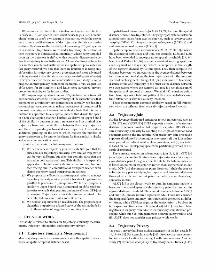
In Fig. 2, there are two trajectories T = [𝑝`1, 𝑝

`

2, 𝑝

`

3] (the black

polyline) and Ta = [𝑝a1, 𝑝a

2, 𝑝a

3] (the red polyline). The solid points

in the trajectories represent the sample points, and they are labeled

with their timestamps, e.g., 𝑝`

1is recorded at 7:00. Using Equation 1,

we can derive a user’s location on T (or Ta ), e.g., at 7:03, the usershould be at 𝑝

`

1′ .

Now we can measure the distance between T and Ta , denotedby 𝑑𝑖𝑠𝑡 (T ,Ta ), at any time 𝑡 as the Euclidean distance. We call this

distance the point distance. STS-Join computes the time duration

where this distance is within a given threshold 𝛿𝑑 .7:00

7:02

7:03

7:107:077:03

7:107:07 7:147:13

7:147:13

Figure 2: Example of trajectories

Trajectories may be generated at different time spans and with

different sampling rates. To compute the point distance between Tand Ta , we need to first define the overlapping time span of segment

pairs. Let 𝑜𝑡 (𝑠`𝑖, 𝑠a𝑗) be the overlapping time span between 𝑠

`

𝑖and

𝑠a𝑗, i.e., [𝑡`

𝑖, 𝑡`

𝑖+1] ∩ [𝑡a𝑗, 𝑡a𝑗+1], where (𝑠

`

𝑖, 𝑠a𝑗) ∈ T × Ta . Denote the

length of the overlapping time span as |𝑜𝑡 (𝑠`𝑖, 𝑠a𝑗) |. Then, in Fig. 2,

𝑜𝑡 (𝑠`1, 𝑠a

1) is [7:02, 7:10], and the length is 8 minutes.

Close-distance duration. When 𝑜𝑡 (𝑠`𝑖, 𝑠a𝑗) ≠ ∅, we call 𝑠`

𝑖and

𝑠a𝑗two time-overlapping segments. Given such segments, we com-

pute the time range [𝑡`a𝑖, 𝑗⊢, 𝑡

`a

𝑖, 𝑗⊣] where 𝑑𝑖𝑠𝑡(T ,Ta ) ⩽ 𝛿𝑑 , i.e.,√(

(XT (𝑡) − XTa (𝑡))2 +

((YT (𝑡) − YTa (𝑡)

)2 ⩽ 𝛿𝑑 (2)

To solve this inequality, we expand Equation 2 with Equation 1

and compute the square of both sides of the inequality:

𝛿2

𝑑⩾

((XT (𝑡) − XTa (𝑡)

)2 +

((YT (𝑡) − YTa (𝑡)

)2

= (𝑘`𝑥 · 𝑡 + 𝑏`𝑥 − 𝑘a𝑥 · 𝑡 − 𝑏a𝑥 )2

+ (𝑘`𝑦 · 𝑡 + 𝑏`𝑦 − 𝑘a𝑦 · 𝑡 − 𝑏a𝑦)2

= [(𝑘`𝑥 − 𝑘a𝑥 )2 + (𝑘`𝑦 − 𝑘a𝑦)2]𝑡2

+ 2[(𝑘`𝑥 − 𝑘a𝑥 ) (𝑏`𝑥 − 𝑏a𝑥 ) + (𝑘

`𝑦 − 𝑘a𝑦) (𝑏

`𝑦 − 𝑏a𝑦)]𝑡

+ (𝑏`𝑥 − 𝑏a𝑥 )2 + (𝑏`𝑦 − 𝑏a𝑦)2,where 𝑡 ∈ 𝑜𝑡 (𝑠

`

𝑖, 𝑠a𝑗 ) and

𝑘`𝑥 =

𝑥`

𝑖+1−𝑥`

𝑖

𝑡`

𝑖+1−𝑡`

𝑖

, 𝑏`𝑥 =

𝑥`

𝑖𝑡`

𝑖+1−𝑥`

𝑖+1𝑡`

𝑖

𝑡`

𝑖+1−𝑡`

𝑖

𝑘a𝑥 =𝑥a𝑗+1−𝑥a

𝑗

𝑡a𝑗+1−𝑡a𝑗

, 𝑏a𝑥 =𝑥a𝑗𝑡a𝑗+1−𝑥a

𝑗+1𝑡a𝑗

𝑡a𝑗+1−𝑡a𝑗

𝑘`𝑦 =

𝑦`

𝑖+1−𝑦`

𝑖

𝑡`

𝑖+1−𝑡`

𝑖

, 𝑏`𝑦 =

𝑦`

𝑖𝑡`

𝑖+1−𝑦`

𝑖+1𝑡`

𝑖

𝑡`

𝑖+1−𝑡`

𝑖

𝑘a𝑦 =𝑦a𝑗+1−𝑦a

𝑗

𝑡a𝑗+1−𝑡a𝑗

, 𝑏a𝑦 =𝑦a𝑗𝑡a𝑗+1−𝑦a

𝑗+1𝑡a𝑗

𝑡a𝑗+1−𝑡a𝑗

(3)

The resultant quadratic inequality has just one variable 𝑡 . It can

be solved straightforwardly by letting the inequality be equal and

computing the roots for the equation with the quadratic formula.

We omit the detailed computation for conciseness.

In Fig. 2, the distance threshold 𝛿𝑑 is represented by the dotted

lines. The distance between the first segments of the two trajecto-

ries first decreases and then increases. At time 𝑡 = 7:03 and 7:07,

SSDBM 2021, July 6–7, 2021, Tampa, FL, USA Yanchuan Chang et al.

𝑑𝑖𝑠𝑡(T ,Ta ) = 𝛿𝑑 . which yields the first time range [7:03, 7:07] that

satisfies 𝛿𝑑 . The distance between the second segments of the two

trajectories keeps decreasing, which reaches 𝛿𝑑 at 7:13. This yields

the second time range [7:13, 7:14] that satisfies 𝛿𝑑 .

We call the length of [𝑡`a𝑖,𝑗⊢, 𝑡

`a

𝑖,𝑗⊣] the close-distance duration (CDD),denoted as 𝑐𝑑𝑑 (𝑠`

𝑖, 𝑠a𝑗) = 𝑡

`a

𝑖, 𝑗⊣ − 𝑡`a

𝑖,𝑗⊢. We define the similarity be-

tween two trajectories as their total CDD across all segments.

Definition 3.1 (Close-distance duration similarity). Given a point

distance threshold 𝛿𝑑 , the close-distance duration similarity (CDDS)

of two trajectories T and Ta , 𝑐𝑑𝑑𝑠 (T ,Ta ), is the sum of 𝑐𝑑𝑑 (𝑠`𝑖, 𝑠a𝑗)

of every time-overlapping segment pair (𝑠`𝑖, 𝑠a𝑗) ∈ T × Ta .

𝑐𝑑𝑑𝑠 (T ,Ta ) =∑

1≤𝑖≤ | T |,1≤ 𝑗≤ |Ta |,𝑜𝑡 (𝑠`𝑖 ,𝑠a𝑗 )≠∅𝑐𝑑𝑑 (𝑠`

𝑖, 𝑠a𝑗 )

(4)

CDDS sums up the duration of all close segments including the

partial ones. This differs from existing trajectory similarity metrics

that require the full trajectories to be close. In Fig. 2, 𝑐𝑑𝑑𝑠 (T ,Ta )equals to the total length of the two time ranges [7:03, 7:07] and

[7:13, 7:14], i.e., 5 minutes.

Problem definition. Now we can formulate our STS-Join.

Definition 3.2 (STS-Join query). Given two trajectory datasets

D𝑝 and D𝑞 , a point distance threshold 𝛿𝑑 , and a close-distance

duration similarity threshold 𝛿𝑡 , STS-Join returns every trajectory

pair (T ,Ta ) ∈ D𝑝 × D𝑞 such that 𝑐𝑑𝑑𝑠 (T ,Ta ) ⩾ 𝛿𝑡 .

4 INDEX STRUCTUREWe assume setD𝑝 to be known (e.g., user trajectory dumps) and set

D𝑞 to be given at query time (e.g., trajectories of newly confirmed

COVID-19 cases). We build an index named STS-Index overD𝑝 such

that D𝑝 can be STS-Joined with D𝑞 efficiently. We use a client-

server architecture to protect location privacy. On a client, a user’s

trajectories are stored in their original form, which are obfuscated

and sent to the server. The obfuscated trajectories from all clients

together are indexed in a tree structure on the server that considers

both their spatial and temporal features. Next, we detail the index

structures on the clients and the server, respectively.

4.1 On Client SideA user’s original trajectories are stored on the client side. We sim-plify and obfuscate an original trajectory before sending it (together

with the client ID and a local trajectory ID) to the server in order to

reduce the communication and protect user’s privacy. We index the

trajectories by their local IDs (e.g., using a sorted array or a B-tree)

for fast retrieval at the refinement stage of query processing.

Trajectory simplification. First, we simplify an original tra-

jectory T by reducing the number of sampled points. This reduces

the storage space and improves the query efficiency later. Our

simplification algorithm is adapted from the Douglas–Peucker al-gorithm (DP) [13]. The native DP algorithm ignores the temporal

dimension. Consider two sampled points 𝑝`

𝑖and 𝑝

`

𝑖+𝑘 (𝑘 > 1) on T .

For all other sampled points between 𝑝`

𝑖and 𝑝

`

𝑖+𝑘 , if their perpen-

dicular distances to the segment between 𝑝`

𝑖and 𝑝

`

𝑖+𝑘 are within a

simplification threshold \𝑠𝑝 (an empirical parameter), then these

points are all removed from T by DP.

In our case, since we interpolate user locations on the trajectory

segments, we require the user location on the simplified segment

𝑝`

𝑖, 𝑝

`

𝑖+𝑘 to be within \𝑠𝑝 distance from that on the original segments

at every time point 𝑡 ∈ [𝑡`𝑖, 𝑡`

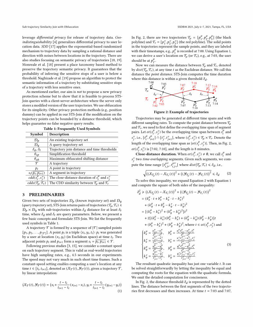
𝑖+𝑘 ]. This guarantees no false negativesin STS-Join over the simplified trajectories. Fig. 3 shows an example.

The original (black) trajectory T has three segments, which is

simplified to just one (red) segment 𝑝˜1, 𝑝

˜4. We compute 𝑝

˜2and

𝑝˜3on 𝑝

˜1, 𝑝

˜4at times 𝑡

`

2and 𝑡

`

3(i.e., the time points of 𝑝

`

2and 𝑝

`

3),

respectively. To ensure valid simplification, the distance between

𝑝`

2and 𝑝

˜2(i.e., 𝑑2) and that between 𝑝

`

3and 𝑝

˜3(i.e., 𝑑3) must both

be within \𝑠𝑝 . This contrasts to the native DP that examines the

perpendicular distances of 𝑝`

2and 𝑝

`

3(i.e., 𝑑⊥

2and 𝑑⊥

3), which are

shorter and may lead to false negatives at query processing.

Figure 3: Example of trajectory simplification

Trajectory obfuscation. Our simplified trajectories retain a

subset of the trajectory points. To protect privacy, we further adapt

the bounded Laplace mechanism (i.e., an algorithm) to obfuscate the

simplified trajectories as inspired by previous studies [14, 16].

The bounded Laplace mechanism adds a noise from the bounded

Laplace distribution to the output of a (query) function. In our

problem, we add a bounded noise to each dimension of a point

on a simplified trajectory to protect users’ location privacy. The

probability distribution function (PDF) of the added noise is [16]:

𝑃𝑟 (𝑥) = _ · 1

2𝑏· exp( −|𝑥 |

𝑏), 𝑥 ∈ [−\𝑜𝑏 , \𝑜𝑏 ] (5)

where _ is a constant,𝑏 is the bias of the distribution, \𝑜𝑏 ∈ R+ is theobfuscated distance threshold. Since the domain of the distribution

is bounded in [−\𝑜𝑏 , \𝑜𝑏 ], the integral of PDF should be 1 for 𝑥 ∈[−\𝑜𝑏 , \𝑜𝑏 ]. This yields the value of _:

_ = (∫ \𝑜𝑏

−\𝑜𝑏

1

2𝑏· exp( −|𝑥 |

𝑏)𝑑𝑥)−1 = (1 − exp(−\𝑜𝑏

𝑏))−1

(6)

We then leverage the inverse cumulative distribution function to

generate random noises that satisfy the PDF. Firstly, we derive the

CDF from the PDF by computing the integral of the PDF for 𝑥 < 0

and 𝑥 ⩾ 0 respectively:

𝐹 (𝑥) ={_2· (exp( 𝑥

𝑏) − exp( −\𝑜𝑏

𝑏)), 𝑥 < 0

1

2+ _

2· (1 − exp( −𝑥

𝑏)), 𝑥 ⩾ 0

(7)

Then, we can obtain the inverse CDF from Equation 7:

𝑥 =

{−𝑏 · ln(1 + _−1 − 2_−1𝑦), 𝑦 ∈ (0, 0.5]𝑏 · ln(1 − _−1 + 2_−1𝑦), 𝑦 ∈ (0.5, 1)

(8)

Here, variable𝑦 is a random number in (0, 1). We generate𝑦 and use

it to obtain noise 𝑥 , which is then added to each point coordinate

of the simplified trajectory. Parameter _ is determined by 𝑏 and \𝑜𝑏(Equation 6), while 𝑏 is the distribution bias.

Sub-trajectory Similarity Join with Obfuscation SSDBM 2021, July 6–7, 2021, Tampa, FL, USA

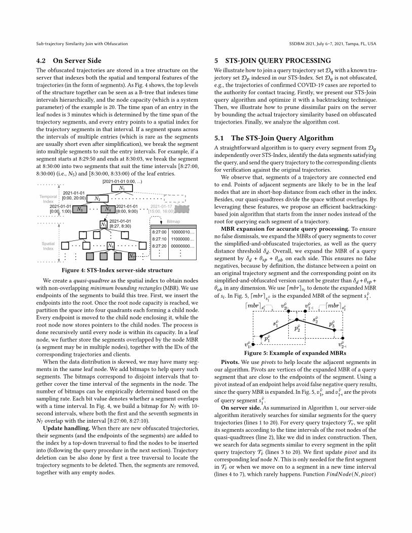
4.2 On Server SideThe obfuscated trajectories are stored in a tree structure on the

server that indexes both the spatial and temporal features of the

trajectories (in the form of segments). As Fig. 4 shows, the top levels

of the structure together can be seen as a B-tree that indexes time

intervals hierarchically, and the node capacity (which is a system

parameter) of the example is 20. The time span of an entry in the

leaf nodes is 3 minutes which is determined by the time span of the

trajectory segments, and every entry points to a spatial index for

the trajectory segments in that interval. If a segment spans across

the intervals of multiple entries (which is rare as the segments

are usually short even after simplification), we break the segment

into multiple segments to suit the entry intervals. For example, if a

segment starts at 8:29:50 and ends at 8:30:03, we break the segment

at 8:30:00 into two segments that suit the time intervals [8:27:00,

8:30:00) (i.e., 𝑁5) and [8:30:00, 8:33:00) of the leaf entries.

2021-01-01[0:00, 1:00)

2021-01-01[8:00, 9:00)

2021-01-17[15:00, 16:00)

2021-01-01[8:27, 8:30)

SpatialIndex

TemporalIndex

BitmapTable

8:27:00 10000010....8:27:10 11000000....8:27:20 00000000....

2021-01-01[0:00, 20:00)

[2021-01-01 0:00, ...)

Figure 4: STS-Index server-side structure

We create a quasi-quadtree as the spatial index to obtain nodes

with non-overlappingminimum bounding rectangles (MBR). We use

endpoints of the segments to build this tree. First, we insert the

endpoints into the root. Once the root node capacity is reached, we

partition the space into four quadrants each forming a child node.

Every endpoint is moved to the child node enclosing it, while the

root node now stores pointers to the child nodes. The process is

done recursively until every node is within its capacity. In a leaf

node, we further store the segments overlapped by the node MBR

(a segment may be in multiple nodes), together with the IDs of the

corresponding trajectories and clients.

When the data distribution is skewed, we may have many seg-

ments in the same leaf node. We add bitmaps to help query such

segments. The bitmaps correspond to disjoint intervals that to-

gether cover the time interval of the segments in the node. The

number of bitmaps can be empirically determined based on the

sampling rate. Each bit value denotes whether a segment overlaps

with a time interval. In Fig. 4, we build a bitmap for 𝑁7 with 10-

second intervals, where both the first and the seventh segments in

𝑁7 overlap with the interval [8:27:00, 8:27:10).

Update handling. When there are new obfuscated trajectories,

their segments (and the endpoints of the segments) are added to

the index by a top-down traversal to find the nodes to be inserted

into (following the query procedure in the next section). Trajectory

deletion can be also done by first a tree traversal to locate the

trajectory segments to be deleted. Then, the segments are removed,

together with any empty nodes.

5 STS-JOIN QUERY PROCESSINGWe illustrate how to join a query trajectory setD𝑞 with a known tra-

jectory set D𝑝 indexed in our STS-Index. Set D𝑞 is not obfuscated,

e.g., the trajectories of confirmed COVID-19 cases are reported to

the authority for contact tracing. Firstly, we present our STS-Join

query algorithm and optimize it with a backtracking technique.

Then, we illustrate how to prune dissimilar pairs on the server

by bounding the actual trajectory similarity based on obfuscated

trajectories. Finally, we analyze the algorithm cost.

5.1 The STS-Join Query AlgorithmA straightforward algorithm is to query every segment from D𝑞

independently over STS-Index, identify the data segments satisfying

the query, and send the query trajectory to the corresponding clients

for verification against the original trajectories.

We observe that, segments of a trajectory are connected end

to end. Points of adjacent segments are likely to be in the leaf

nodes that are in short-hop distance from each other in the index.

Besides, our quasi-quadtrees divide the space without overlaps. By

leveraging these features, we propose an efficient backtracking-

based join algorithm that starts from the inner nodes instead of the

root for querying each segment of a trajectory.

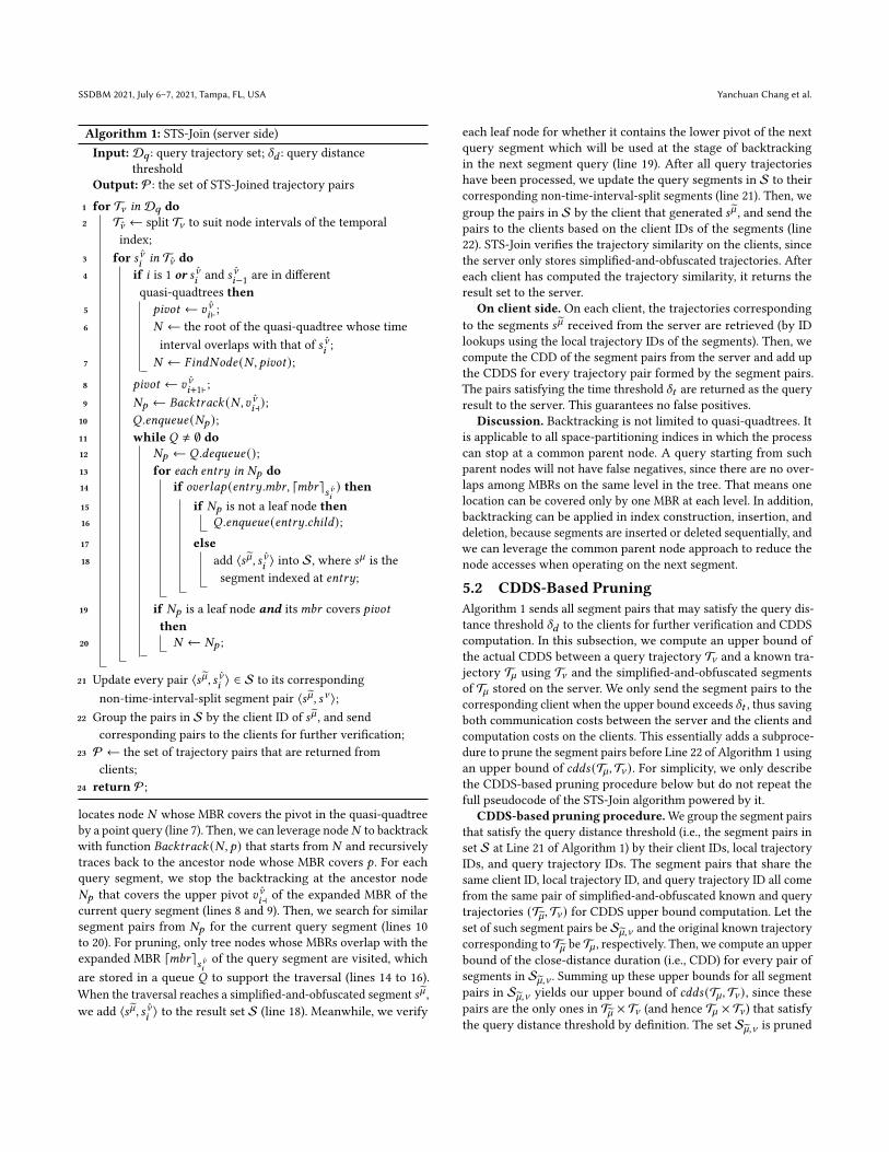
MBR expansion for accurate query processing. To ensure

no false dismissals, we expand the MBRs of query segments to cover

the simplified-and-obfuscated trajectories, as well as the query

distance threshold 𝛿𝑑 . Overall, we expand the MBR of a query

segment by 𝛿𝑑 + \𝑠𝑝 + \𝑜𝑏 on each side. This ensures no false

negatives, because by definition, the distance between a point on

an original trajectory segment and the corresponding point on its

simplified-and-obfuscated version cannot be greater than 𝛿𝑑 +\𝑠𝑝 +\𝑜𝑏 in any dimension. We use ⌈𝑚𝑏𝑟⌉𝑠𝑖 to denote the expanded MBR

of 𝑠𝑖 . In Fig. 5, ⌈𝑚𝑏𝑟⌉𝑠 a

1

is the expanded MBR of the segment 𝑠 a1.

Figure 5: Example of expanded MBRsPivots. We use pivots to help locate the adjacent segments in

our algorithm. Pivots are vertices of the expanded MBR of a query

segment that are close to the endpoints of the segment. Using a

pivot instead of an endpoint helps avoid false negative query results,

since the queryMBR is expanded. In Fig. 5, 𝑣 a1⊢ and 𝑣

a1⊣ are the pivots

of query segment 𝑠 a1.

On server side. As summarized in Algorithm 1, our server-side

algorithm iteratively searches for similar segments for the query

trajectories (lines 1 to 20). For every query trajectory Ta , we splitits segments according to the time intervals of the root nodes of the

quasi-quadtrees (line 2), like we did in index construction. Then,

we search for data segments similar to every segment in the split

query trajectory Ta (lines 3 to 20). We first update 𝑝𝑖𝑣𝑜𝑡 and its

corresponding leaf node𝑁 . This is only needed for the first segment

in Ta or when we move on to a segment in a new time interval

(lines 4 to 7), which rarely happens. Function 𝐹𝑖𝑛𝑑𝑁𝑜𝑑𝑒 (𝑁, 𝑝𝑖𝑣𝑜𝑡)

SSDBM 2021, July 6–7, 2021, Tampa, FL, USA Yanchuan Chang et al.

Algorithm 1: STS-Join (server side)

Input: D𝑞 : query trajectory set; 𝛿𝑑 : query distance

threshold

Output: P: the set of STS-Joined trajectory pairs

1 for Ta in D𝑞 do2 Ta ← split Ta to suit node intervals of the temporal

index;

3 for 𝑠 a𝑖in Ta do

4 if 𝑖 is 1 or 𝑠 a𝑖and 𝑠 a

𝑖−1are in different

quasi-quadtrees then5 𝑝𝑖𝑣𝑜𝑡 ← 𝑣 a

𝑖⊢;6 𝑁 ← the root of the quasi-quadtree whose time

interval overlaps with that of 𝑠 a𝑖;

7 𝑁 ← 𝐹𝑖𝑛𝑑𝑁𝑜𝑑𝑒 (𝑁, 𝑝𝑖𝑣𝑜𝑡);8 𝑝𝑖𝑣𝑜𝑡 ← 𝑣 a

𝑖+1⊢;9 𝑁𝑝 ← 𝐵𝑎𝑐𝑘𝑡𝑟𝑎𝑐𝑘 (𝑁, 𝑣 a

𝑖⊣);10 𝑄.𝑒𝑛𝑞𝑢𝑒𝑢𝑒 (𝑁𝑝 );11 while 𝑄 ≠ ∅ do12 𝑁𝑝 ← 𝑄.𝑑𝑒𝑞𝑢𝑒𝑢𝑒 ();13 for each 𝑒𝑛𝑡𝑟𝑦 in 𝑁𝑝 do14 if 𝑜𝑣𝑒𝑟𝑙𝑎𝑝 (𝑒𝑛𝑡𝑟𝑦.𝑚𝑏𝑟, ⌈𝑚𝑏𝑟⌉

𝑠 a𝑖) then

15 if 𝑁𝑝 is not a leaf node then16 𝑄.𝑒𝑛𝑞𝑢𝑒𝑢𝑒 (𝑒𝑛𝑡𝑟𝑦.𝑐ℎ𝑖𝑙𝑑);17 else18 add ⟨𝑠˜, 𝑠 a

𝑖⟩ into S, where 𝑠` is the

segment indexed at 𝑒𝑛𝑡𝑟𝑦;

19 if 𝑁𝑝 is a leaf node and its𝑚𝑏𝑟 covers 𝑝𝑖𝑣𝑜𝑡

then20 𝑁 ← 𝑁𝑝 ;

21 Update every pair ⟨𝑠˜, 𝑠 a𝑖⟩ ∈ S to its corresponding

non-time-interval-split segment pair ⟨𝑠˜, 𝑠a ⟩;22 Group the pairs in S by the client ID of 𝑠˜, and send

corresponding pairs to the clients for further verification;

23 P ← the set of trajectory pairs that are returned from

clients;

24 return P;

locates node 𝑁 whose MBR covers the pivot in the quasi-quadtree

by a point query (line 7). Then, we can leverage node𝑁 to backtrack

with function 𝐵𝑎𝑐𝑘𝑡𝑟𝑎𝑐𝑘 (𝑁, 𝑝) that starts from 𝑁 and recursively

traces back to the ancestor node whose MBR covers 𝑝 . For each

query segment, we stop the backtracking at the ancestor node

𝑁𝑝 that covers the upper pivot 𝑣 a𝑖⊣ of the expanded MBR of the

current query segment (lines 8 and 9). Then, we search for similar

segment pairs from 𝑁𝑝 for the current query segment (lines 10

to 20). For pruning, only tree nodes whose MBRs overlap with the

expanded MBR ⌈𝑚𝑏𝑟⌉𝑠 a𝑖of the query segment are visited, which

are stored in a queue 𝑄 to support the traversal (lines 14 to 16).

When the traversal reaches a simplified-and-obfuscated segment 𝑠˜,we add ⟨𝑠˜, 𝑠 a

𝑖⟩ to the result set S (line 18). Meanwhile, we verify

each leaf node for whether it contains the lower pivot of the next

query segment which will be used at the stage of backtracking

in the next segment query (line 19). After all query trajectories

have been processed, we update the query segments in S to their

corresponding non-time-interval-split segments (line 21). Then, we

group the pairs in S by the client that generated 𝑠˜, and send the

pairs to the clients based on the client IDs of the segments (line

22). STS-Join verifies the trajectory similarity on the clients, since

the server only stores simplified-and-obfuscated trajectories. After

each client has computed the trajectory similarity, it returns the

result set to the server.

On client side. On each client, the trajectories corresponding

to the segments 𝑠˜ received from the server are retrieved (by ID

lookups using the local trajectory IDs of the segments). Then, we

compute the CDD of the segment pairs from the server and add up

the CDDS for every trajectory pair formed by the segment pairs.

The pairs satisfying the time threshold 𝛿𝑡 are returned as the query

result to the server. This guarantees no false positives.

Discussion. Backtracking is not limited to quasi-quadtrees. It

is applicable to all space-partitioning indices in which the process

can stop at a common parent node. A query starting from such

parent nodes will not have false negatives, since there are no over-

laps among MBRs on the same level in the tree. That means one

location can be covered only by one MBR at each level. In addition,

backtracking can be applied in index construction, insertion, and

deletion, because segments are inserted or deleted sequentially, and

we can leverage the common parent node approach to reduce the

node accesses when operating on the next segment.

5.2 CDDS-Based PruningAlgorithm 1 sends all segment pairs that may satisfy the query dis-

tance threshold 𝛿𝑑 to the clients for further verification and CDDS

computation. In this subsection, we compute an upper bound of

the actual CDDS between a query trajectory Ta and a known tra-

jectory T using Ta and the simplified-and-obfuscated segments

of T stored on the server. We only send the segment pairs to the

corresponding client when the upper bound exceeds 𝛿𝑡 , thus saving

both communication costs between the server and the clients and

computation costs on the clients. This essentially adds a subproce-

dure to prune the segment pairs before Line 22 of Algorithm 1 using

an upper bound of 𝑐𝑑𝑑𝑠 (T ,Ta ). For simplicity, we only describe

the CDDS-based pruning procedure below but do not repeat the

full pseudocode of the STS-Join algorithm powered by it.

CDDS-based pruning procedure.We group the segment pairs

that satisfy the query distance threshold (i.e., the segment pairs in

set S at Line 21 of Algorithm 1) by their client IDs, local trajectory

IDs, and query trajectory IDs. The segment pairs that share the

same client ID, local trajectory ID, and query trajectory ID all come

from the same pair of simplified-and-obfuscated known and query

trajectories (T ,Ta ) for CDDS upper bound computation. Let the

set of such segment pairs be S˜,a and the original known trajectory

corresponding to T be T , respectively. Then, we compute an upper

bound of the close-distance duration (i.e., CDD) for every pair of

segments in S˜,a . Summing up these upper bounds for all segment

pairs in S˜,a yields our upper bound of 𝑐𝑑𝑑𝑠 (T ,Ta ), since thesepairs are the only ones in T × Ta (and hence T × Ta ) that satisfythe query distance threshold by definition. The set S˜,a is pruned

Sub-trajectory Similarity Join with Obfuscation SSDBM 2021, July 6–7, 2021, Tampa, FL, USA

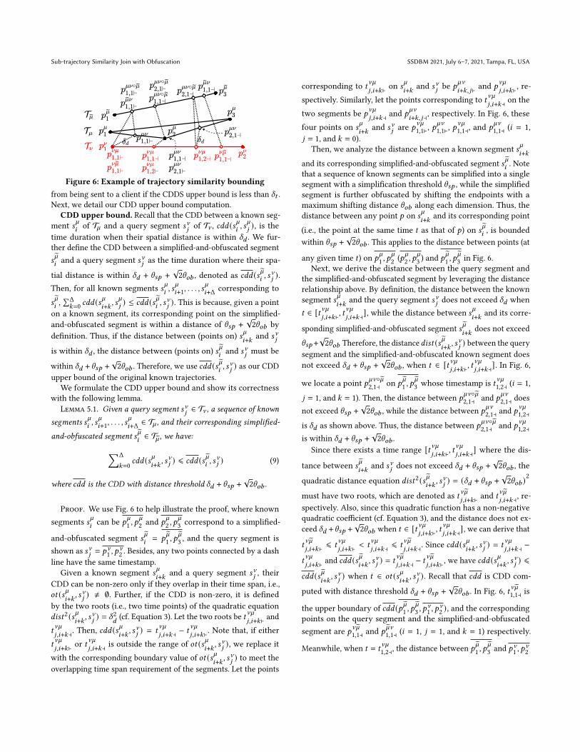
Figure 6: Example of trajectory similarity boundingfrom being sent to a client if the CDDS upper bound is less than 𝛿𝑡 .

Next, we detail our CDD upper bound computation.

CDD upper bound. Recall that the CDD between a known seg-

ment 𝑠`

𝑖of T and a query segment 𝑠a

𝑗of Ta , 𝑐𝑑𝑑 (𝑠`𝑖 , 𝑠

`

𝑗), is the

time duration when their spatial distance is within 𝛿𝑑 . We fur-

ther define the CDD between a simplified-and-obfuscated segment

𝑠˜𝑖and a query segment 𝑠a

𝑗as the time duration where their spa-

tial distance is within 𝛿𝑑 + \𝑠𝑝 +√

2\𝑜𝑏 , denoted as 𝑐𝑑𝑑 (𝑠˜𝑖, 𝑠a𝑗).

Then, for all known segments 𝑠`

𝑖, 𝑠`

𝑖+1, . . . , 𝑠`

𝑖+Δ corresponding to

𝑠˜𝑖,

∑Δ𝑘=0

𝑐𝑑𝑑 (𝑠`𝑖+𝑘 , 𝑠

`

𝑗) ≤ 𝑐𝑑𝑑 (𝑠˜

𝑖, 𝑠a𝑗). This is because, given a point

on a known segment, its corresponding point on the simplified-

and-obfuscated segment is within a distance of \𝑠𝑝 +√

2\𝑜𝑏 by

definition. Thus, if the distance between (points on) 𝑠`

𝑖+𝑘 and 𝑠a𝑗

is within 𝛿𝑑 , the distance between (points on) 𝑠˜𝑖and 𝑠a

𝑗must be

within 𝛿𝑑 + \𝑠𝑝 +√

2\𝑜𝑏 . Therefore, we use 𝑐𝑑𝑑 (𝑠˜𝑖, 𝑠a𝑗) as our CDD

upper bound of the original known trajectories.

We formulate the CDD upper bound and show its correctness

with the following lemma.

Lemma 5.1. Given a query segment 𝑠a𝑗∈ Ta , a sequence of known

segments 𝑠`𝑖, 𝑠`

𝑖+1, . . . , 𝑠`

𝑖+Δ ∈ T , and their corresponding simplified-

and-obfuscated segment 𝑠˜𝑖∈ T , we have:∑Δ

𝑘=0

𝑐𝑑𝑑 (𝑠`𝑖+𝑘 , 𝑠

a𝑗 ) ⩽ 𝑐𝑑𝑑 (𝑠˜

𝑖, 𝑠a𝑗 ) (9)

where 𝑐𝑑𝑑 is the CDD with distance threshold 𝛿𝑑 + \𝑠𝑝 +√

2\𝑜𝑏 .

Proof. We use Fig. 6 to help illustrate the proof, where known

segments 𝑠`

𝑖can be 𝑝

`

1, 𝑝

`

2and 𝑝

`

2, 𝑝

`

3correspond to a simplified-

and-obfuscated segment 𝑠˜𝑖

= 𝑝˜1, 𝑝

˜3, and the query segment is

shown as 𝑠a𝑗= 𝑝a

1, 𝑝a

2. Besides, any two points connected by a dash

line have the same timestamp.

Given a known segment 𝑠`

𝑖+𝑘 and a query segment 𝑠a𝑗, their

CDD can be non-zero only if they overlap in their time span, i.e.,

𝑜𝑡 (𝑠`𝑖+𝑘 , 𝑠

a𝑗) ≠ ∅. Further, if the CDD is non-zero, it is defined

by the two roots (i.e., two time points) of the quadratic equation

𝑑𝑖𝑠𝑡2 (𝑠`𝑖+𝑘 , 𝑠

a𝑗) = 𝛿2

𝑑(cf. Equation 3). Let the two roots be 𝑡

a`

𝑗,𝑖+𝑘⊢ and

𝑡a`

𝑗,𝑖+𝑘⊣. Then, 𝑐𝑑𝑑 (𝑠`

𝑖+𝑘 , 𝑠a𝑗) = 𝑡

a`

𝑗,𝑖+𝑘⊣ − 𝑡a`

𝑗,𝑖+𝑘⊢. Note that, if either

𝑡a`

𝑗,𝑖+𝑘⊢ or 𝑡a`

𝑗,𝑖+𝑘⊣ is outside the range of 𝑜𝑡 (𝑠`

𝑖+𝑘 , 𝑠a𝑗), we replace it

with the corresponding boundary value of 𝑜𝑡 (𝑠`𝑖+𝑘 , 𝑠

a𝑗) to meet the

overlapping time span requirement of the segments. Let the points

corresponding to 𝑡a`

𝑗,𝑖+𝑘⊢ on 𝑠`

𝑖+𝑘 and 𝑠a𝑗be 𝑝

`a

𝑖+𝑘,𝑗⊢ and 𝑝a`

𝑗,𝑖+𝑘⊢, re-

spectively. Similarly, let the points corresponding to 𝑡a`

𝑗,𝑖+𝑘⊣ on the

two segments be 𝑝a`

𝑗,𝑖+𝑘⊣ and 𝑝`a

𝑖+𝑘,𝑗⊣, respectively. In Fig. 6, these

four points on 𝑠`

𝑖+𝑘 and 𝑠a𝑗are 𝑝

a`

1,1⊢, 𝑝`a

1,1⊢, 𝑝a`

1,1⊣, and 𝑝`a

1,1⊣ (𝑖 = 1,

𝑗 = 1, and 𝑘 = 0).

Then, we analyze the distance between a known segment 𝑠`

𝑖+𝑘and its corresponding simplified-and-obfuscated segment 𝑠

˜𝑖. Note

that a sequence of known segments can be simplified into a single

segment with a simplification threshold \𝑠𝑝 , while the simplified

segment is further obfuscated by shifting the endpoints with a

maximum shifting distance \𝑜𝑏 along each dimension. Thus, the

distance between any point 𝑝 on 𝑠`

𝑖+𝑘 and its corresponding point

(i.e., the point at the same time 𝑡 as that of 𝑝) on 𝑠˜𝑖, is bounded

within \𝑠𝑝 +√

2\𝑜𝑏 . This applies to the distance between points (at

any given time 𝑡 ) on 𝑝`

1, 𝑝

`

2(𝑝

`

2, 𝑝

`

3) and 𝑝

˜1, 𝑝

˜3in Fig. 6.

Next, we derive the distance between the query segment and

the simplified-and-obfuscated segment by leveraging the distance

relationship above. By definition, the distance between the known

segment 𝑠`

𝑖+𝑘 and the query segment 𝑠a𝑗does not exceed 𝛿𝑑 when

𝑡 ∈ [𝑡a`𝑗,𝑖+𝑘⊢, 𝑡

a`

𝑗,𝑖+𝑘⊣], while the distance between 𝑠`

𝑖+𝑘 and its corre-

sponding simplified-and-obfuscated segment 𝑠˜𝑖+𝑘 does not exceed

\𝑠𝑝 +√

2\𝑜𝑏 Therefore, the distance𝑑𝑖𝑠𝑡 (𝑠˜𝑖+𝑘 , 𝑠

a𝑗) between the query

segment and the simplified-and-obfuscated known segment does

not exceed 𝛿𝑑 + \𝑠𝑝 +√

2\𝑜𝑏 , when 𝑡 ∈ [𝑡a`𝑗,𝑖+𝑘⊢, 𝑡

a`

𝑗,𝑖+𝑘⊣]. In Fig. 6,

we locate a point 𝑝`a◦˜2,1⊣ on 𝑝

˜1, 𝑝

˜3whose timestamp is 𝑡

a`

1,2⊣ (𝑖 = 1,

𝑗 = 1, and 𝑘 = 1). Then, the distance between 𝑝`a◦˜2,1⊣ and 𝑝

`a

2,1⊣ does

not exceed \𝑠𝑝 +√

2\𝑜𝑏 , while the distance between 𝑝`a

2,1⊣ and 𝑝a`

1,2⊣is 𝛿𝑑 as shown above. Thus, the distance between 𝑝

`a◦˜2,1⊣ and 𝑝

a`

1,2⊣is within 𝛿𝑑 + \𝑠𝑝 +

√2\𝑜𝑏 .

Since there exists a time range [𝑡a`𝑗,𝑖+𝑘⊢, 𝑡

a`

𝑗,𝑖+𝑘⊣] where the dis-

tance between 𝑠˜𝑖+𝑘 and 𝑠a

𝑗does not exceed 𝛿𝑑 + \𝑠𝑝 +

√2\𝑜𝑏 , the

quadratic distance equation 𝑑𝑖𝑠𝑡2 (𝑠˜𝑖+𝑘 , 𝑠

a𝑗) = (𝛿𝑑 + \𝑠𝑝 +

√2\𝑜𝑏 )

2

must have two roots, which are denoted as 𝑡a˜𝑗,𝑖+𝑘⊢ and 𝑡

a˜𝑗,𝑖+𝑘⊣, re-

spectively. Also, since this quadratic function has a non-negative

quadratic coefficient (cf. Equation 3), and the distance does not ex-

ceed 𝛿𝑑 +\𝑠𝑝 +√

2\𝑜𝑏 when 𝑡 ∈ [𝑡a`𝑗,𝑖+𝑘⊢, 𝑡

a`

𝑗,𝑖+𝑘⊣], we can derive that

𝑡a˜𝑗,𝑖+𝑘⊢ ⩽ 𝑡

a`

𝑗,𝑖+𝑘⊢ < 𝑡a`

𝑗,𝑖+𝑘⊣ ⩽ 𝑡a˜𝑗,𝑖+𝑘⊣. Since 𝑐𝑑𝑑 (𝑠

`

𝑖+𝑘 , 𝑠a𝑗) = 𝑡

a`

𝑗,𝑖+𝑘⊣ −

𝑡a`

𝑗,𝑖+𝑘⊢ and 𝑐𝑑𝑑 (𝑠˜𝑖+𝑘 , 𝑠

a𝑗) = 𝑡

a˜𝑗,𝑖+𝑘⊣ − 𝑡

a˜𝑗,𝑖+𝑘⊢, we have 𝑐𝑑𝑑 (𝑠

`

𝑖+𝑘 , 𝑠a𝑗) ⩽

𝑐𝑑𝑑 (𝑠˜𝑖+𝑘 , 𝑠

a𝑗) when 𝑡 ∈ 𝑜𝑡 (𝑠`

𝑖+𝑘 , 𝑠a𝑗). Recall that 𝑐𝑑𝑑 is CDD com-

puted with distance threshold 𝛿𝑑 + \𝑠𝑝 +√

2\𝑜𝑏 . In Fig. 6, 𝑡a˜1,1⊣ is

the upper boundary of 𝑐𝑑𝑑 (𝑝˜1, 𝑝

˜3, 𝑝a

1, 𝑝a

2), and the corresponding

points on the query segment and the simplified-and-obfuscated

segment are 𝑝a˜1,1⊣ and 𝑝

˜a1,1⊣ (𝑖 = 1, 𝑗 = 1, and 𝑘 = 1) respectively.

Meanwhile, when 𝑡 = 𝑡a`

1,2⊣, the distance between 𝑝˜1, 𝑝

˜3and 𝑝a

1, 𝑝a

2

SSDBM 2021, July 6–7, 2021, Tampa, FL, USA Yanchuan Chang et al.

does not exceed 𝛿𝑑 + \𝑠𝑝 +√

2\𝑜𝑏 . Thus, we have 𝑡a`

1,2⊣ ⩽ 𝑡a˜1,1⊣. Such

an inequality is also applicable to other CDD boundaries.

Finally, we sum up the CDD of each segment in 𝑠`

𝑖, 𝑠`

𝑖+1, . . . , 𝑠`

𝑖+Δwith 𝑠a

𝑗, and we sum up 𝑐𝑑𝑑 (𝑠˜

𝑖, 𝑠a𝑗) that corresponds to different

time ranges in 𝑜𝑡 (𝑠`𝑖+𝑘 , 𝑠

a𝑗) where 0 ⩽ 𝑘 ⩽ Δ. Since the inequality

is satisfied on each separate time range, such inequality is also sat-

isfied for the sums, i.e., 𝑐𝑑𝑑 (𝑝`1, 𝑝

`

2, 𝑝a

1, 𝑝a

2) + 𝑐𝑑𝑑 (𝑝`

2, 𝑝

`

3, 𝑝a

1, 𝑝a

2) ⩽

𝑐𝑑𝑑 (𝑝˜1, 𝑝

˜3, 𝑝a

1, 𝑝a

2) in Fig. 6. This completes the proof. □

Given Lemma 5.1, we have the following lemma to bound the

CDDS for the original known trajectories.

Lemma 5.2. Given a query trajectory Ta , a known trajectory T ,and its corresponding simplified-and-obfuscated version T , we have:

𝑐𝑑𝑑𝑠 (T ,Ta ) ⩽ 𝑐𝑑𝑑𝑠 (T ,Ta ) (10)

where 𝑐𝑑𝑑𝑠 is CDDS with distance threshold 𝛿𝑑 + \𝑠𝑝 +√

2\𝑜𝑏 .

Proof. The proof is straightforward and hence is omitted. □

5.3 Cost AnalysisWe analyze the cost of Algorithm 1 in terms of the number of

node accesses. If a query segment spans the whole spatio-temporal

space (worst case), all index nodes may be visited, with or without

backtracking. However, this rarely happens. Inmany cities, points of

interest are distributed in a polycentric structure [7, 12]. Trajectories

are likely to gather near local centers, where backtracking helps

query the sub-spatial index of the centers.

The algorithm iterates through the query segments. In each

iteration, the costs are spent on finding the common parent node

of two adjacent points (and hence adjacent segments) in the query

trajectory and on traversing the index to reach leaf nodes.

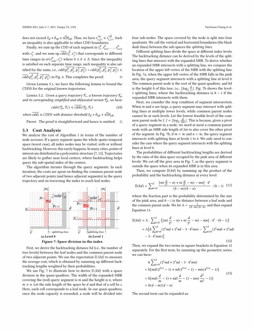
(a) Level 0 (b) Level 1

Figure 7: Space division in the index

First, we derive the backtracking distance 𝑏𝑑 (i.e., the number of

tree levels) between the leaf nodes and the common parent node

of two adjacent points. We use the expectation E (𝑏𝑑) to measure

the average cost, which is obtained by summing up different back-

tracking lengths weighted by their probabilities.

We use Fig. 7 to illustrate how to derive E (𝑏𝑑) with a space

division in the quasi-quadtree. The width of the expanded MBR

covering the (red) query segment is𝑚 and the height is 𝑛, where

𝑚 ⩾ 𝑛. Let the side length of the space be 𝑑 and that of a cell be 𝑐 .

Here, each cell corresponds to a leaf node. In our quasi-quadtree,

once the node capacity is exceeded, a node will be divided into

four sub-nodes. The space covered by the node is split into four

quadrants. We call the vertical and horizontal boundaries (the black

dash lines) between the sub-spaces the splitting lines.Different splitting lines divide the space at different index levels.

The backtracking distance can be derived by the levels of the split-

ting lines that intersect with the expanded MBR. To derive whether

an expanded MBR intersects with a splitting line, we compare the

location of the upper left vertex of the MBR with the splitting line.

In Fig. 7a, when the upper left vertex of the MBR falls in the pink

area, the query segment intersects with a splitting line at level 0.

The common parent node is the root of the quasi-quadtree, and 𝑏𝑑

is the height ℎ of this tree, i.e., ⌊log2

𝑑𝑐 ⌋. Fig. 7b shows the level-

1 splitting lines, where the backtracking distance is ℎ − 1 if the

expanded MBR intersects with them.

Next, we consider the stop condition of segment intersection.

When𝑚 and 𝑛 are large, a query segment may intersect with split-

ting lines at multiple lower levels, while common parent nodes

cannot be at such levels. Let the lowest feasible level of the com-

mon parent node be 𝐼 , 𝐼 = ⌊log2

𝑑2𝑚 ⌋. This is because, given a pivot

of a query segment in a node, we need at most a common parent

node with an MBR side length of 2𝑚 to also cover the other pivot

of the segment. In Fig. 7b, if𝑚 > 4𝑐 and 𝑛 > 4𝑐 , the query segment

intersects with splitting lines at levels 1 to 4. We only need to con-

sider the case where the query segment intersects with the splitting

lines at level 0.

The probabilities of different backtracking lengths are derived

by the ratio of the data space occupied by the pink area of different

levels. We cut off the grey area in Fig. 7, as the query segment is

outside the space when its expanded MBR is in this area.

Then, we compute E(𝑏𝑑) by summing up the product of the

probability and the backtracking distance at every level:

E(𝑏𝑑) =∑𝐼

𝑖=0

[𝑚( 𝑑2𝑖 − 𝑛) + 𝑛( 𝑑

2𝑖 −𝑚) −𝑚𝑛] · 4𝑖

(𝑏 −𝑚) (𝑏 − 𝑛) · (ℎ − 𝑖) (11)

where the fraction part is the probability determined by the size

of the pink area, and ℎ − 𝑖 is the distance between a leaf node and

the common parent node. We let Λ = 1

(𝑏−𝑚) (𝑏−𝑛) and then expand

Equation 11:

E(𝑏𝑑) = Λ ·∑𝐼

𝑖=0

{[𝑚( 𝑑

2𝑖− 𝑛) + 𝑛( 𝑑

2𝑖−𝑚) −𝑚𝑛] · 4𝑖 · (ℎ − 𝑖)

}= Λ

[ℎ∑𝐼

𝑖=0

(2𝑖𝑚𝑑 + 2𝑖𝑛𝑑 − 3 · 4𝑖𝑚𝑛) −

∑𝐼

𝑖=0

(2𝑖𝑚𝑑𝑖 + 2𝑖𝑛𝑑𝑖

− 3 · 4𝑖𝑚𝑛𝑖)]

(12)

Then, we expand the two terms in square brackets in Equation 12

separately. For the first term, by summing up the geometric series,

we can have:

ℎ∑𝐼

𝑖=0

(2𝑖𝑚𝑑 + 2𝑖𝑛𝑑 − 3 · 4𝑖𝑚𝑛)

= ℎ[𝑚𝑑 (2𝐼+1 − 1) + 𝑛𝑑 (2𝐼+1 − 1) −𝑚𝑛(4𝐼+1 − 1)]

= ℎ[𝑚𝑑 ( 𝑑𝑚− 1) + 𝑛𝑑 ( 𝑑

𝑚− 1) −𝑚𝑛( 𝑑

2

𝑚2− 1)]

= ℎ(𝑑 −𝑚) (𝑑 − 𝑛)

(13)

The second term can be expanded as:

Sub-trajectory Similarity Join with Obfuscation SSDBM 2021, July 6–7, 2021, Tampa, FL, USA∑𝐼

𝑖=0

(2𝑖𝑚𝑑𝑖 + 2𝑖𝑛𝑑𝑖 − 3 · 4𝑖𝑚𝑛𝑖)

= 2𝐼 (𝑑 −𝑚) (𝑑 − 𝑛) − (𝐼 + 1)∑𝐼

𝑖=1

(2𝑖𝑚𝑑 + 2𝑖𝑛𝑑 − 3 · 4𝑖𝑚𝑛)

= 2𝐼 (𝑑 −𝑚) (𝑑 − 𝑛) − (𝐼 + 1) (𝑑 − 2𝑚) (𝑑 − 2𝑛)

(14)

Lastly, we plug Equation 13, 14 into Equation 12:

E(𝑏𝑑) = Λ[ℎ(𝑑 −𝑚) (𝑑 − 𝑛) − 2𝐼 (𝑑 −𝑚) (𝑑 − 𝑛)

+ (𝐼 + 1) (𝑑 − 2𝑚) (𝑑 − 2𝑛)]

= ℎ − 2𝐼 + (𝐼 + 1) (𝑑 − 2𝑚) (𝑑 − 2𝑛)(𝑑 −𝑚) (𝑑 − 𝑛)

⩽ ℎ − 𝐼 + 1

(15)

So far, we have that E (𝑏𝑑) is up to ℎ − 𝐼 + 1.

Total cost. To query a trajectory, STS-Join iteratively takes

𝑂 ((ℎ−𝐼 ) ¯|T |) node accesses for backtracking, since only one node isvisited at each level, where

¯|T | is the number of segments in a query

trajectory. Besides, it visits 𝑂 (4ℎ−𝐼 ¯|T |) nodes while searching forsimilar segments of a query segment. In total, the cost of STS-Join

with backtracking is 𝑂 (4ℎ−𝐼 ¯|T | |D𝑞 |).

6 EXPERIMENTS6.1 Experimental SetupAll experiments are conducted on a 64-bit machine running Ubuntu

20.04 LTS with a 6-core AMD Ryzen 5 CPU, 32 GB RAM, and a

500GB SSD. All algorithms are implemented in C++ and run in

main memory.

Datasets. To the best of our knowledge, there is no public

contact-tracing datasets. We use two real trajectory datasets in-

stead: DiDi [2] and GeoLife [1]. DiDi contains vehicle trajectoriesin Chengdu, a capital city in China. We randomly sample trajec-

tories recorded in the first week of November, 2016 to generate

a dataset with 500k trajectories and 67.7 million segments (this

is limited by our memory size). The trajectories come from 201k

users (each is considered a client in the experiments), i.e., there

are 2.5 trajectories per client on average. There are 135 segments

per trajectory on average. The average length and time span of a

segment are 30.0 meters and 4.5 seconds, respectively.

GeoLife contains trajectories of different transport modes (e.g.,

walking, driving, and cycling) recorded mainly in Beijing, China.

We only keep the trajectories within the Fifth Ring Road of Beijing.

There are some 11k trajectories in this area and very few outside.

We randomly sample 10k trajectories from them to form the GeoLife

dataset used in the experiments. We shift the trajectory times into

the same week without changing their time span to increase the

density in time. The trajectories come from 182 users (clients), i.e.,

there are 55 trajectories per client on average. There are 9.0 million

segments in these trajectories and 896 segments per trajectory

on average. The average length and time span of a segment are

12.2 meters and 9.2 seconds, respectively. The two datasets are

summarized in Table 2. We further generate their random subsets

for scalability tests. See Table 3 for the sizes of the subsets.

Algorithms. There is no existing algorithm for STS-Join. We

adapt two techniques which result in three baseline algorithms.

Meanwhile, we replace the join predicates in these algorithms with

ours, so all algorithms return the same accurate query results. We test

three variants of our proposed STS-Join algorithm to confirm the

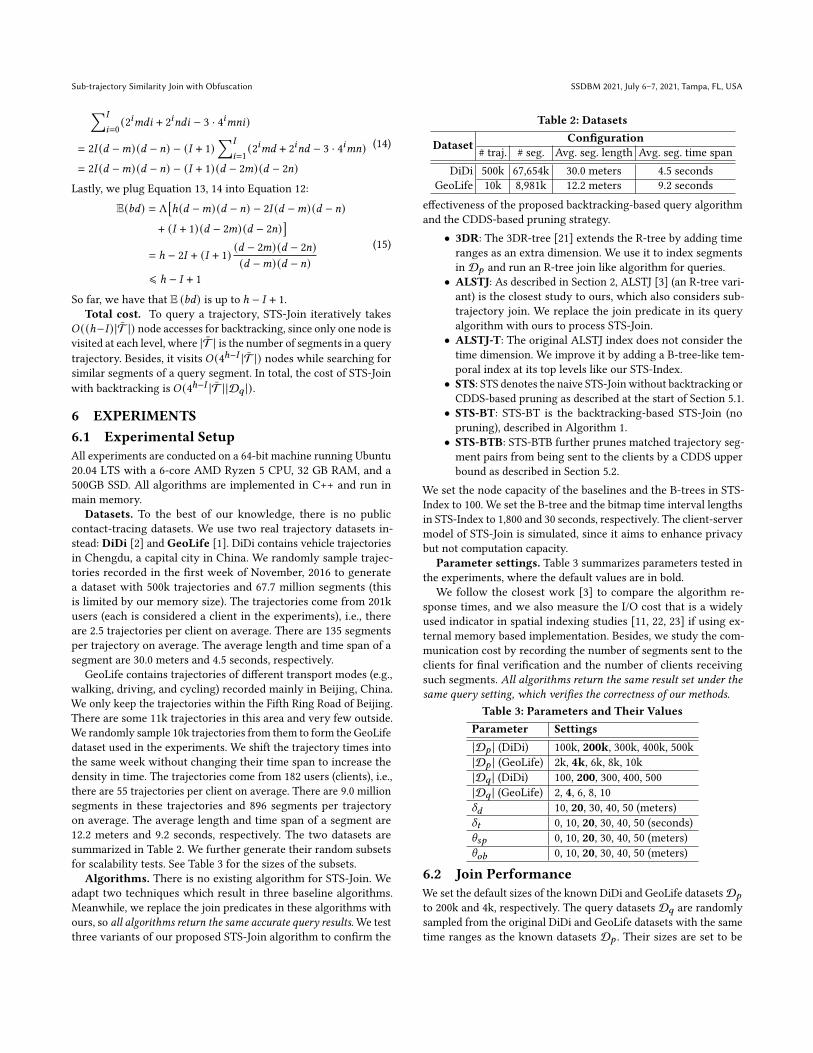
Table 2: Datasets

Dataset Configuration# traj. # seg. Avg. seg. length Avg. seg. time span

DiDi 500k 67,654k 30.0 meters 4.5 seconds

GeoLife 10k 8,981k 12.2 meters 9.2 seconds

effectiveness of the proposed backtracking-based query algorithm

and the CDDS-based pruning strategy.

• 3DR: The 3DR-tree [21] extends the R-tree by adding time

ranges as an extra dimension. We use it to index segments

in D𝑝 and run an R-tree join like algorithm for queries.

• ALSTJ: As described in Section 2, ALSTJ [3] (an R-tree vari-

ant) is the closest study to ours, which also considers sub-

trajectory join. We replace the join predicate in its query

algorithm with ours to process STS-Join.

• ALSTJ-T: The original ALSTJ index does not consider thetime dimension. We improve it by adding a B-tree-like tem-

poral index at its top levels like our STS-Index.

• STS: STS denotes the naive STS-Join without backtracking orCDDS-based pruning as described at the start of Section 5.1.

• STS-BT: STS-BT is the backtracking-based STS-Join (no

pruning), described in Algorithm 1.

• STS-BTB: STS-BTB further prunes matched trajectory seg-

ment pairs from being sent to the clients by a CDDS upper

bound as described in Section 5.2.

We set the node capacity of the baselines and the B-trees in STS-

Index to 100. We set the B-tree and the bitmap time interval lengths

in STS-Index to 1,800 and 30 seconds, respectively. The client-server

model of STS-Join is simulated, since it aims to enhance privacy

but not computation capacity.

Parameter settings. Table 3 summarizes parameters tested in

the experiments, where the default values are in bold.

We follow the closest work [3] to compare the algorithm re-

sponse times, and we also measure the I/O cost that is a widely

used indicator in spatial indexing studies [11, 22, 23] if using ex-

ternal memory based implementation. Besides, we study the com-

munication cost by recording the number of segments sent to the

clients for final verification and the number of clients receiving

such segments. All algorithms return the same result set under thesame query setting, which verifies the correctness of our methods.

Table 3: Parameters and Their ValuesParameter Settings|D𝑝 | (DiDi) 100k, 200k, 300k, 400k, 500k|D𝑝 | (GeoLife) 2k, 4k, 6k, 8k, 10k|D𝑞 | (DiDi) 100, 200, 300, 400, 500|D𝑞 | (GeoLife) 2, 4, 6, 8, 10𝛿𝑑 10, 20, 30, 40, 50 (meters)

𝛿𝑡 0, 10, 20, 30, 40, 50 (seconds)\𝑠𝑝 0, 10, 20, 30, 40, 50 (meters)

\𝑜𝑏 0, 10, 20, 30, 40, 50 (meters)

6.2 Join PerformanceWe set the default sizes of the known DiDi and GeoLife datasetsD𝑝

to 200k and 4k, respectively. The query datasets D𝑞 are randomly

sampled from the original DiDi and GeoLife datasets with the same

time ranges as the known datasets D𝑝 . Their sizes are set to be

SSDBM 2021, July 6–7, 2021, Tampa, FL, USA Yanchuan Chang et al.

proportional to those of the respective known DiDi and GeoLife

datasets. The default sizes of DiDi and GeoLife query datasets

are 200 and 4 (i.e., 0.1% of |D𝑝 |), respectively. The GeoLife querydatasets might seem small, but there are some 900 segments per

trajectory on average, which are sufficient to show the performance

difference of the algorithms.

10-1

100

101

102

103

100k 200k 300k 400k 500k

Tim

e /

s

Dataset size

3DR

ALSTJ

ALSTJ-T

STS

STS-BT

STS-BTB

(a) Response time (DiDi)

105

106

107

108

109

100k 200k 300k 400k 500k

# n

od

e a

cce

sse

s

Dataset size

3DR

ALSTJ

ALSTJ-T

STS

STS-BT

STS-BTB

(b) Number of node accesses (DiDi)

10-2

10-1

100

101

102

2k 4k 6k 8k 10k

Tim

e /

s

Dataset size

3DR

ALSTJ

ALSTJ-T

STS

STS-BT

STS-BTB

(c) Response time (GeoLife)

103

104

105

106

107

2k 4k 6k 8k 10k

# n

od

e a

cce

sse

s

Dataset size

3DR

ALSTJ

ALSTJ-T

STS

STS-BT

STS-BTB

(d) Number of node accesses (GeoLife)

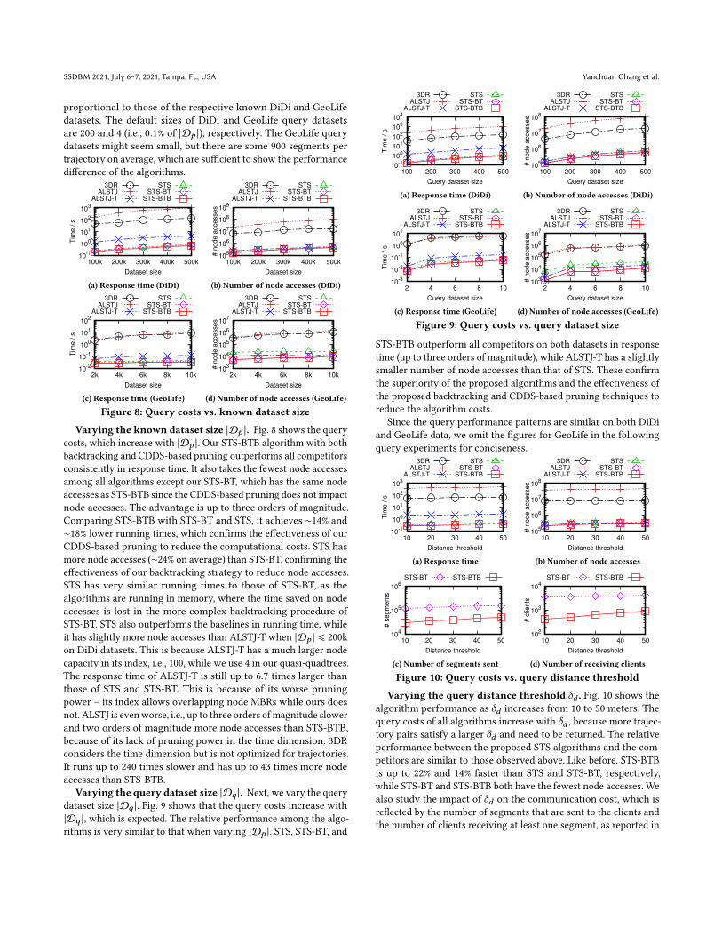
Figure 8: Query costs vs. known dataset size

Varying the known dataset size |D𝑝 |. Fig. 8 shows the querycosts, which increase with |D𝑝 |. Our STS-BTB algorithm with both

backtracking and CDDS-based pruning outperforms all competitors

consistently in response time. It also takes the fewest node accesses

among all algorithms except our STS-BT, which has the same node

accesses as STS-BTB since the CDDS-based pruning does not impact

node accesses. The advantage is up to three orders of magnitude.

Comparing STS-BTB with STS-BT and STS, it achieves ∼14% and

∼18% lower running times, which confirms the effectiveness of our

CDDS-based pruning to reduce the computational costs. STS has

more node accesses (∼24% on average) than STS-BT, confirming the

effectiveness of our backtracking strategy to reduce node accesses.

STS has very similar running times to those of STS-BT, as the

algorithms are running in memory, where the time saved on node

accesses is lost in the more complex backtracking procedure of

STS-BT. STS also outperforms the baselines in running time, while

it has slightly more node accesses than ALSTJ-T when |D𝑝 | ⩽ 200k

on DiDi datasets. This is because ALSTJ-T has a much larger node

capacity in its index, i.e., 100, while we use 4 in our quasi-quadtrees.

The response time of ALSTJ-T is still up to 6.7 times larger than

those of STS and STS-BT. This is because of its worse pruning

power – its index allows overlapping node MBRs while ours does

not. ALSTJ is evenworse, i.e., up to three orders ofmagnitude slower

and two orders of magnitude more node accesses than STS-BTB,

because of its lack of pruning power in the time dimension. 3DR

considers the time dimension but is not optimized for trajectories.

It runs up to 240 times slower and has up to 43 times more node

accesses than STS-BTB.

Varying the query dataset size |D𝑞 |. Next, we vary the querydataset size |D𝑞 |. Fig. 9 shows that the query costs increase with

|D𝑞 |, which is expected. The relative performance among the algo-

rithms is very similar to that when varying |D𝑝 |. STS, STS-BT, and

10-1

100

101

102

103

104

100 200 300 400 500

Tim

e /

s

Query dataset size

3DRALSTJ

ALSTJ-T

STSSTS-BT

STS-BTB

(a) Response time (DiDi)

105

106

107

108

100 200 300 400 500

# n

od

e a

cce

sse

s

Query dataset size

3DRALSTJ

ALSTJ-T

STSSTS-BT

STS-BTB

(b) Number of node accesses (DiDi)

10-3

10-2

10-1

100

101

2 4 6 8 10

Tim

e /

s

Query dataset size

3DRALSTJ

ALSTJ-T

STSSTS-BT

STS-BTB

(c) Response time (GeoLife)

103

104

105

106

107

2 4 6 8 10

# n

od

e a

cce

sse

s

Query dataset size

3DRALSTJ

ALSTJ-T

STSSTS-BT

STS-BTB

(d) Number of node accesses (GeoLife)

Figure 9: Query costs vs. query dataset size

STS-BTB outperform all competitors on both datasets in response

time (up to three orders of magnitude), while ALSTJ-T has a slightly

smaller number of node accesses than that of STS. These confirm

the superiority of the proposed algorithms and the effectiveness of

the proposed backtracking and CDDS-based pruning techniques to

reduce the algorithm costs.

Since the query performance patterns are similar on both DiDi

and GeoLife data, we omit the figures for GeoLife in the following

query experiments for conciseness.

10-1

100

101

102

103

10 20 30 40 50

Tim

e /

s

Distance threshold

3DR

ALSTJ

ALSTJ-T

STS

STS-BT

STS-BTB

(a) Response time

105

106

107

108

10 20 30 40 50

# n

od

e a

cce

sse

s

Distance threshold

3DR

ALSTJ

ALSTJ-T

STS

STS-BT

STS-BTB

(b) Number of node accesses

104

105

106

10 20 30 40 50

# s

eg

me

nts

Distance threshold

STS-BT STS-BTB

(c) Number of segments sent

102

103

104

10 20 30 40 50

# c

lie

nts

Distance threshold

STS-BT STS-BTB

(d) Number of receiving clients

Figure 10: Query costs vs. query distance threshold

Varying the query distance threshold 𝛿𝑑 . Fig. 10 shows thealgorithm performance as 𝛿𝑑 increases from 10 to 50 meters. The

query costs of all algorithms increase with 𝛿𝑑 , because more trajec-

tory pairs satisfy a larger 𝛿𝑑 and need to be returned. The relative

performance between the proposed STS algorithms and the com-

petitors are similar to those observed above. Like before, STS-BTB

is up to 22% and 14% faster than STS and STS-BT, respectively,

while STS-BT and STS-BTB both have the fewest node accesses. We

also study the impact of 𝛿𝑑 on the communication cost, which is

reflected by the number of segments that are sent to the clients and

the number of clients receiving at least one segment, as reported in

Sub-trajectory Similarity Join with Obfuscation SSDBM 2021, July 6–7, 2021, Tampa, FL, USA

Figs. 10c and 10d, respectively. We see that, while the communica-

tion costs of STS-BTB increase with 𝛿𝑑 which is expected, they are

at least 3.1 and 4.8 times lower than those of STS-BT (for 𝛿𝑑 ≤ 50)

in terms of the number of segments sent and the number of clients

receiving the segments, respectively. Here, STS has been omitted

since it has the same communication costs as STS-BT, and the

same applies to the figures below. The results further confirm the

effectiveness of our CDDS-based pruning.

10-1

100

101

102

103

0 10 20 30 40 50

Tim

e /

s

Duration threshold

3DR

ALSTJ

ALSTJ-T

STS

STS-BT

STS-BTB

(a) Response time

105

106

107

108

0 10 20 30 40 50

# n

od

e a

cce

sse

s

Duration threshold

3DR

ALSTJ

ALSTJ-T

STS

STS-BT

STS-BTB

(b) Number of node accesses

104

105

106

0 10 20 30 40 50

# s

eg

me

nts

Duration threshold

STS-BT STS-BTB

(c) Number of segments sent

102

103

104

0 10 20 30 40 50

# c

lie

nts

Duration threshold

STS-BT STS-BTB

(d) Number of receiving clients

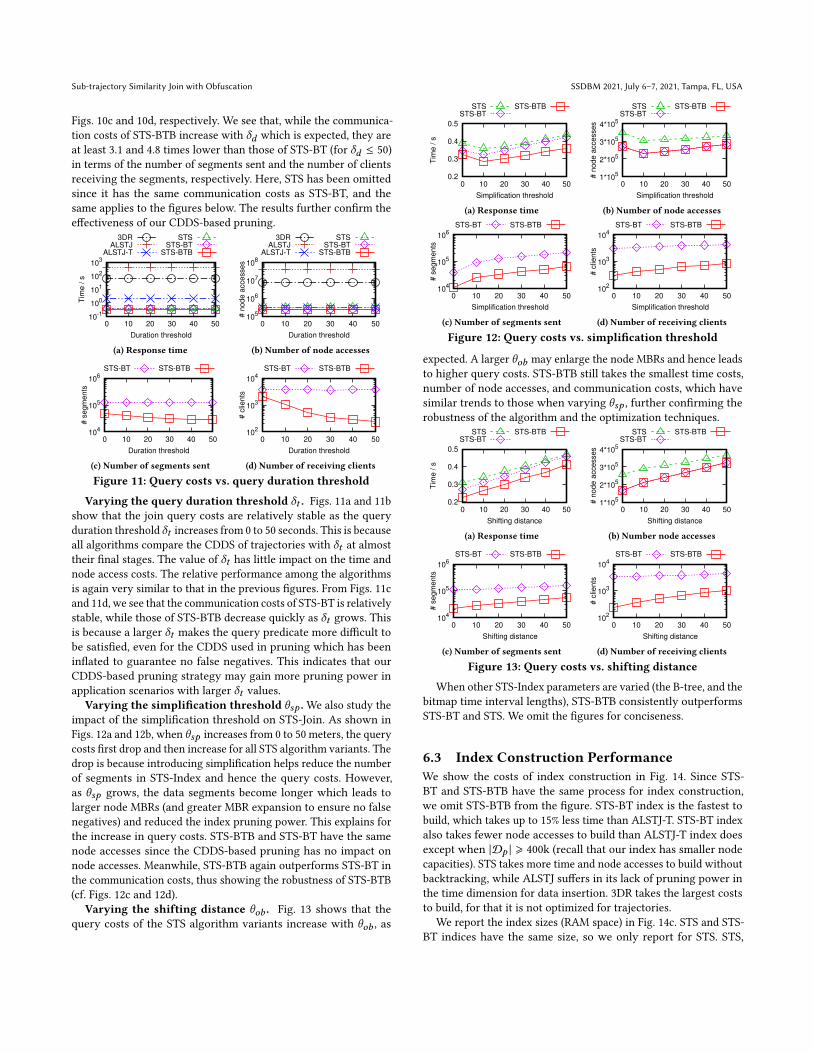
Figure 11: Query costs vs. query duration threshold

Varying the query duration threshold 𝛿𝑡 . Figs. 11a and 11b

show that the join query costs are relatively stable as the query

duration threshold 𝛿𝑡 increases from 0 to 50 seconds. This is because

all algorithms compare the CDDS of trajectories with 𝛿𝑡 at almost

their final stages. The value of 𝛿𝑡 has little impact on the time and

node access costs. The relative performance among the algorithms

is again very similar to that in the previous figures. From Figs. 11c

and 11d, we see that the communication costs of STS-BT is relatively

stable, while those of STS-BTB decrease quickly as 𝛿𝑡 grows. This

is because a larger 𝛿𝑡 makes the query predicate more difficult to

be satisfied, even for the CDDS used in pruning which has been

inflated to guarantee no false negatives. This indicates that our

CDDS-based pruning strategy may gain more pruning power in

application scenarios with larger 𝛿𝑡 values.

Varying the simplification threshold \𝑠𝑝 .We also study the

impact of the simplification threshold on STS-Join. As shown in

Figs. 12a and 12b, when \𝑠𝑝 increases from 0 to 50 meters, the query

costs first drop and then increase for all STS algorithm variants. The

drop is because introducing simplification helps reduce the number

of segments in STS-Index and hence the query costs. However,

as \𝑠𝑝 grows, the data segments become longer which leads to

larger node MBRs (and greater MBR expansion to ensure no false

negatives) and reduced the index pruning power. This explains for

the increase in query costs. STS-BTB and STS-BT have the same

node accesses since the CDDS-based pruning has no impact on

node accesses. Meanwhile, STS-BTB again outperforms STS-BT in

the communication costs, thus showing the robustness of STS-BTB

(cf. Figs. 12c and 12d).

Varying the shifting distance \𝑜𝑏 . Fig. 13 shows that the

query costs of the STS algorithm variants increase with \𝑜𝑏 , as

0.2

0.3

0.4

0.5

0 10 20 30 40 50

Tim

e /

s

Simplification threshold

STSSTS-BT

STS-BTB

(a) Response time

1*105

2*105

3*105

4*105

0 10 20 30 40 50

# n

od

e a

cce

sse

s

Simplification threshold

STSSTS-BT

STS-BTB

(b) Number of node accesses

104

105

106

0 10 20 30 40 50

# s

eg

me

nts

Simplification threshold

STS-BT STS-BTB

(c) Number of segments sent

102

103

104

0 10 20 30 40 50

# c

lien

ts

Simplification threshold

STS-BT STS-BTB

(d) Number of receiving clients

Figure 12: Query costs vs. simplification threshold

expected. A larger \𝑜𝑏 may enlarge the node MBRs and hence leads

to higher query costs. STS-BTB still takes the smallest time costs,

number of node accesses, and communication costs, which have

similar trends to those when varying \𝑠𝑝 , further confirming the

robustness of the algorithm and the optimization techniques.

0.2

0.3

0.4

0.5

0 10 20 30 40 50

Tim

e /

s

Shifting distance

STSSTS-BT

STS-BTB

(a) Response time

1*105

2*105

3*105

4*105

0 10 20 30 40 50

# n

od

e a

cce

sse

s

Shifting distance

STSSTS-BT

STS-BTB

(b) Number node accesses

104

105

106

0 10 20 30 40 50

# s

eg

me

nts

Shifting distance

STS-BT STS-BTB

(c) Number of segments sent

102

103

104

0 10 20 30 40 50

# c

lien

ts

Shifting distance

STS-BT STS-BTB

(d) Number of receiving clients

Figure 13: Query costs vs. shifting distance

When other STS-Index parameters are varied (the B-tree, and the

bitmap time interval lengths), STS-BTB consistently outperforms

STS-BT and STS. We omit the figures for conciseness.

6.3 Index Construction PerformanceWe show the costs of index construction in Fig. 14. Since STS-

BT and STS-BTB have the same process for index construction,

we omit STS-BTB from the figure. STS-BT index is the fastest to

build, which takes up to 15% less time than ALSTJ-T. STS-BT index

also takes fewer node accesses to build than ALSTJ-T index does

except when |D𝑝 | ⩾ 400k (recall that our index has smaller node

capacities). STS takes more time and node accesses to build without

backtracking, while ALSTJ suffers in its lack of pruning power in

the time dimension for data insertion. 3DR takes the largest costs

to build, for that it is not optimized for trajectories.

We report the index sizes (RAM space) in Fig. 14c. STS and STS-

BT indices have the same size, so we only report for STS. STS,

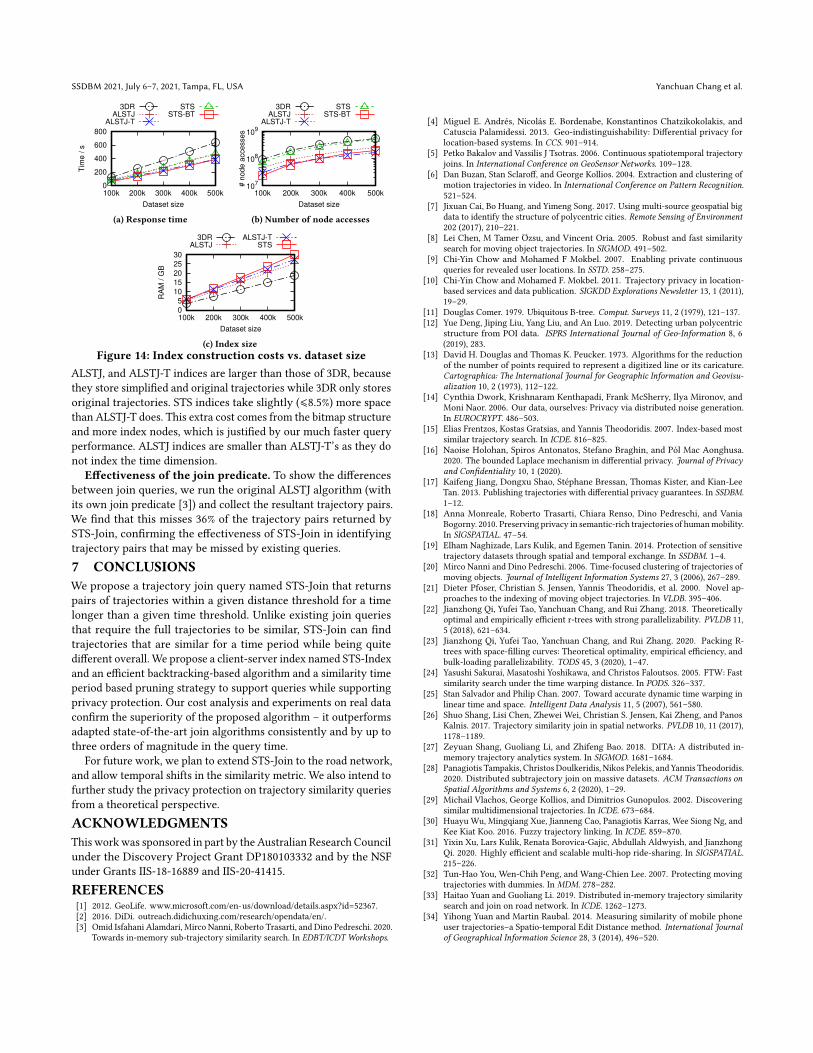
SSDBM 2021, July 6–7, 2021, Tampa, FL, USA Yanchuan Chang et al.

0

200

400

600

800

100k 200k 300k 400k 500k

Tim

e /

s

Dataset size

3DR

ALSTJ

ALSTJ-T

STS

STS-BT

(a) Response time

107

108

109

100k 200k 300k 400k 500k

# n

od

e a

cce

sse

s

Dataset size

3DR

ALSTJ

ALSTJ-T

STS

STS-BT

(b) Number of node accesses

0

5

10

15

20

25

30

100k 200k 300k 400k 500k

RA

M /

GB

Dataset size

3DR

ALSTJ

ALSTJ-T

STS

(c) Index sizeFigure 14: Index construction costs vs. dataset size

ALSTJ, and ALSTJ-T indices are larger than those of 3DR, because

they store simplified and original trajectories while 3DR only stores

original trajectories. STS indices take slightly (⩽8.5%) more space

than ALSTJ-T does. This extra cost comes from the bitmap structure

and more index nodes, which is justified by our much faster query

performance. ALSTJ indices are smaller than ALSTJ-T’s as they do

not index the time dimension.

Effectiveness of the join predicate. To show the differences

between join queries, we run the original ALSTJ algorithm (with

its own join predicate [3]) and collect the resultant trajectory pairs.

We find that this misses 36% of the trajectory pairs returned by

STS-Join, confirming the effectiveness of STS-Join in identifying

trajectory pairs that may be missed by existing queries.

7 CONCLUSIONSWe propose a trajectory join query named STS-Join that returns

pairs of trajectories within a given distance threshold for a time

longer than a given time threshold. Unlike existing join queries

that require the full trajectories to be similar, STS-Join can find

trajectories that are similar for a time period while being quite

different overall. We propose a client-server index named STS-Index

and an efficient backtracking-based algorithm and a similarity time

period based pruning strategy to support queries while supporting

privacy protection. Our cost analysis and experiments on real data

confirm the superiority of the proposed algorithm – it outperforms

adapted state-of-the-art join algorithms consistently and by up to

three orders of magnitude in the query time.

For future work, we plan to extend STS-Join to the road network,

and allow temporal shifts in the similarity metric. We also intend to

further study the privacy protection on trajectory similarity queries

from a theoretical perspective.

ACKNOWLEDGMENTSThis workwas sponsored in part by the Australian Research Council

under the Discovery Project Grant DP180103332 and by the NSF

under Grants IIS-18-16889 and IIS-20-41415.

REFERENCES[1] 2012. GeoLife. www.microsoft.com/en-us/download/details.aspx?id=52367.

[2] 2016. DiDi. outreach.didichuxing.com/research/opendata/en/.

[3] Omid Isfahani Alamdari, Mirco Nanni, Roberto Trasarti, and Dino Pedreschi. 2020.

Towards in-memory sub-trajectory similarity search. In EDBT/ICDT Workshops.

[4] Miguel E. Andrés, Nicolás E. Bordenabe, Konstantinos Chatzikokolakis, and

Catuscia Palamidessi. 2013. Geo-indistinguishability: Differential privacy for

location-based systems. In CCS. 901–914.[5] Petko Bakalov and Vassilis J Tsotras. 2006. Continuous spatiotemporal trajectory

joins. In International Conference on GeoSensor Networks. 109–128.[6] Dan Buzan, Stan Sclaroff, and George Kollios. 2004. Extraction and clustering of

motion trajectories in video. In International Conference on Pattern Recognition.521–524.

[7] Jixuan Cai, Bo Huang, and Yimeng Song. 2017. Using multi-source geospatial big

data to identify the structure of polycentric cities. Remote Sensing of Environment202 (2017), 210–221.

[8] Lei Chen, M Tamer Özsu, and Vincent Oria. 2005. Robust and fast similarity

search for moving object trajectories. In SIGMOD. 491–502.[9] Chi-Yin Chow and Mohamed F Mokbel. 2007. Enabling private continuous

queries for revealed user locations. In SSTD. 258–275.[10] Chi-Yin Chow and Mohamed F. Mokbel. 2011. Trajectory privacy in location-

based services and data publication. SIGKDD Explorations Newsletter 13, 1 (2011),19–29.

[11] Douglas Comer. 1979. Ubiquitous B-tree. Comput. Surveys 11, 2 (1979), 121–137.[12] Yue Deng, Jiping Liu, Yang Liu, and An Luo. 2019. Detecting urban polycentric

structure from POI data. ISPRS International Journal of Geo-Information 8, 6

(2019), 283.

[13] David H. Douglas and Thomas K. Peucker. 1973. Algorithms for the reduction

of the number of points required to represent a digitized line or its caricature.

Cartographica: The International Journal for Geographic Information and Geovisu-alization 10, 2 (1973), 112–122.

[14] Cynthia Dwork, Krishnaram Kenthapadi, Frank McSherry, Ilya Mironov, and

Moni Naor. 2006. Our data, ourselves: Privacy via distributed noise generation.

In EUROCRYPT. 486–503.[15] Elias Frentzos, Kostas Gratsias, and Yannis Theodoridis. 2007. Index-based most

similar trajectory search. In ICDE. 816–825.[16] Naoise Holohan, Spiros Antonatos, Stefano Braghin, and Pól Mac Aonghusa.

2020. The bounded Laplace mechanism in differential privacy. Journal of Privacyand Confidentiality 10, 1 (2020).

[17] Kaifeng Jiang, Dongxu Shao, Stéphane Bressan, Thomas Kister, and Kian-Lee

Tan. 2013. Publishing trajectories with differential privacy guarantees. In SSDBM.

1–12.

[18] Anna Monreale, Roberto Trasarti, Chiara Renso, Dino Pedreschi, and Vania

Bogorny. 2010. Preserving privacy in semantic-rich trajectories of humanmobility.

In SIGSPATIAL. 47–54.[19] Elham Naghizade, Lars Kulik, and Egemen Tanin. 2014. Protection of sensitive

trajectory datasets through spatial and temporal exchange. In SSDBM. 1–4.

[20] Mirco Nanni and Dino Pedreschi. 2006. Time-focused clustering of trajectories of

moving objects. Journal of Intelligent Information Systems 27, 3 (2006), 267–289.[21] Dieter Pfoser, Christian S. Jensen, Yannis Theodoridis, et al. 2000. Novel ap-

proaches to the indexing of moving object trajectories. In VLDB. 395–406.[22] Jianzhong Qi, Yufei Tao, Yanchuan Chang, and Rui Zhang. 2018. Theoretically

optimal and empirically efficient r-trees with strong parallelizability. PVLDB 11,

5 (2018), 621–634.

[23] Jianzhong Qi, Yufei Tao, Yanchuan Chang, and Rui Zhang. 2020. Packing R-

trees with space-filling curves: Theoretical optimality, empirical efficiency, and

bulk-loading parallelizability. TODS 45, 3 (2020), 1–47.[24] Yasushi Sakurai, Masatoshi Yoshikawa, and Christos Faloutsos. 2005. FTW: Fast

similarity search under the time warping distance. In PODS. 326–337.[25] Stan Salvador and Philip Chan. 2007. Toward accurate dynamic time warping in

linear time and space. Intelligent Data Analysis 11, 5 (2007), 561–580.[26] Shuo Shang, Lisi Chen, Zhewei Wei, Christian S. Jensen, Kai Zheng, and Panos

Kalnis. 2017. Trajectory similarity join in spatial networks. PVLDB 10, 11 (2017),

1178–1189.

[27] Zeyuan Shang, Guoliang Li, and Zhifeng Bao. 2018. DITA: A distributed in-

memory trajectory analytics system. In SIGMOD. 1681–1684.[28] Panagiotis Tampakis, Christos Doulkeridis, Nikos Pelekis, and Yannis Theodoridis.

2020. Distributed subtrajectory join on massive datasets. ACM Transactions onSpatial Algorithms and Systems 6, 2 (2020), 1–29.

[29] Michail Vlachos, George Kollios, and Dimitrios Gunopulos. 2002. Discovering

similar multidimensional trajectories. In ICDE. 673–684.[30] Huayu Wu, Mingqiang Xue, Jianneng Cao, Panagiotis Karras, Wee Siong Ng, and

Kee Kiat Koo. 2016. Fuzzy trajectory linking. In ICDE. 859–870.[31] Yixin Xu, Lars Kulik, Renata Borovica-Gajic, Abdullah Aldwyish, and Jianzhong

Qi. 2020. Highly efficient and scalable multi-hop ride-sharing. In SIGSPATIAL.215–226.

[32] Tun-Hao You, Wen-Chih Peng, and Wang-Chien Lee. 2007. Protecting moving

trajectories with dummies. In MDM. 278–282.

[33] Haitao Yuan and Guoliang Li. 2019. Distributed in-memory trajectory similarity

search and join on road network. In ICDE. 1262–1273.[34] Yihong Yuan and Martin Raubal. 2014. Measuring similarity of mobile phone

user trajectories–a Spatio-temporal Edit Distance method. International Journalof Geographical Information Science 28, 3 (2014), 496–520.