Study on Tidal Resonance in Severn Estuary and Bristol Channel

1

Study on Tidal Resonance in Severn Estuary and Bristol Channel 1

2

Dongfang Liang *, §, Junqiang Xia †, Roger A Falconer ‡ and Jingxin Zhang * 3

4

5

* State Key Laboratory of Ocean Engineering, School of Naval Architecture, Ocean and 6

Civil Engineering, Shanghai Jiao Tong University, Shanghai 200240, China 7

8

† State Key Laboratory of Water Resources and Hydropower Engineering Science, 9

Wuhan University, Wuhan 430072, China 10

11

‡ Cardiff School of Engineering, Cardiff University, 12

The Parade, Cardiff CF24 3AA, UK 13

14

§ [email protected] 15

16

2

Abstract 17

A horizontal hydrodynamic model was applied to predict the response characteristics 18

of the Severn Estuary and Bristol Channel to regular long waves, in an effort to gain 19

insight into the tidal behaviour of this area. A boundary-fitted curvilinear mesh of high 20

resolution was generated, covering the downstream reach of the River Severn, the 21

Severn Estuary and the Bristol Channel, with the seaward boundary set from Milford 22

Haven to Hartland Point on the west and the riverine boundary at Gloucester towards 23

the east. The simulation was first calibrated against the observed tidal levels and 24

currents at various sites, for typical spring and neap tides. Subsequently, water surface 25

oscillations inside the domain were excited by sinusoidal long waves of different 26

periods at the open boundary to find the fundamental mode of oscillation. The 27

amplitude-frequency relationships were calculated at numerous sites. It was found that 28

the primary resonant mode of oscillation in the Severn Estuary occurred at the tidal 29

period of around 8 hours. Although not exactly coinciding with this resonant mode, the 30

M2 tide still observed a relatively high amplification factor, which helps explain why 31

this water body experiences one of the largest tidal ranges in the world. 32

33

Keywords: Long waves; Tide; Severn Estuary; Bristol Channel; Resonance 34

35

1. Introduction 36

The Severn Estuary is situated between South East Wales and South West England 37

and forms the mouth of the River Severn, which is the longest river in the UK. 38

Conventionally, the River Severn is identified as the Severn Estuary after either the 39

Severn Bridge (M48 Bridge) or the second Severn Crossing (M4 Bridge), both south of 40

3

Gloucestershire. However, the normal tidal limit is at Maisemore on the West Channel 41

just north of Gloucester, and at Llanthony Weir on the East Channel. The lower limit of 42

the Estuary is defined by a transection connecting Lavernock Point to the south of 43

Cardiff and Sand Point near Weston-super-Mare, which is near to the proposed site for 44

the Cardiff-Weston Barrage. The Estuary is about 3.2 km wide at the M48 Bridge, and 45

about 14 km wide between Cardiff and Weston-super-Mare. The Severn Estuary 46

discharges into the Bristol Channel, which then discharges into the Irish Sea and the 47

wider North Atlantic Ocean. The Channel is over 50 km across at its widest point, with 48

an average angle of latitude of around 51.35o. 49

The Bristol Channel and Severn Estuary constitute one of the largest, semi-enclosed 50

water basins in the UK. The Severn Estuary is well known for having a large tidal 51

range, regarded as one of the highest in the world and one of the most famous fluvial 52

landmarks in Europe. The dominant component is the principal lunar M2 tide. The 53

typical mean spring tidal range is 12.2 m, with the high spring tidal range approaching 54

14.0 m at Avonmouth, located just upstream of the port of Bristol. There are large areas 55

of intertidal mudflats, and the spring tidal currents in the Estuary are in excess of 2 m/s. 56

Such high tidal ranges make the Estuary a famous scenic spot, and also place it at the 57

centre of the widely publicised and controversial debate concerning the large-scale 58

development of the marine renewable energy. The hydrodynamic processes in the 59

Bristol Channel and Severn Estuary have been studied extensively (e.g. Uncles, 1981; 60

Kirby and Shaw, 2005; Falconer et al., 2009; Xia et al., 2010a, 2010b). 61

Not much research can be found on the underlying nature of the tidal behaviour in the 62

Severn Estuary and Bristol Channel. Some researchers have attributed the high tidal 63

range to the funnel shape and continuously upward slope of the basin (e.g. Pan et al. 64

4

2007). The contraction in width from the mouth to the head concentrates the tidal 65

energy, and the shallowing effect due to the reduction in the water depth forces the 66

wave height to rise. However, it has long been pointed out by Marmer (1922) that even 67

the combination of those two effects is not enough to produce the enormous tidal ranges 68

observed in reality. Marmer (1922) used the standing wave theory to explain the natural 69

resonance in the Bay of Fundy, Canada, which boasts the world’s largest tidal range. It 70

was concluded that the tidal period was very close to the natural period of oscillation in 71

the Bay of Fundy, which was the primary reason for its high tides. Previous approaches 72

in deriving the natural period of oscillation of a water body are often crude. Marmer 73

(1922) simply estimated according to the characteristic scales of the problem. 74

Proudman (1953) took a constant-depth assumption. Xing et al. (2008) based their 75

numerical estimation on the mild slope equation in the frequency domain, which 76

disregard the bottom friction and Coriolis effects. 77

This paper aims to ascertain the natural oscillation period and amplification factor of 78

the Severn Estuary and Bristol Channel through a time-domain study, based on a fully-79

dynamic shallow water solver (Liang et al. 2007a, 2007b, Liang et al. 2013). One 80

challenge of the present numerical simulation is the coexistence of multiple scales. On 81

the seaward side, the flow expands as wide as over 100 km; on the upstream side, the 82

river is as narrow as less than 50 m at some sections. Typically, the semidiurnal tidal 83

period is around half a day, so the time to be simulated needs to be tens or hundreds of 84

hours long in order to capture the harmonic dynamics. Corresponding to such a long 85

period, the tidal wavelength can be hundreds of kilometres. Yet, the steep water level 86

rise in front of the river tidal bore can be accomplished over just tens of meters, i.e. 87

several times the river depth, which may pass a river section in less than 1 minute. Such 88

5

a disparity in spatial and temporal scales by several orders of magnitude poses an 89

obstacle to numerical simulations. Moreover, natural topographies are inherently 90

complex and irregular, making it difficult to accurately represent them. 91

The paper first set up a computational model for the Severn Estuary and Bristol 92

Channel based on the shallow water equations, which was then calibrated and validated 93

by comparing the predictions with field observations. Subsequently, this model was 94

used to examine the frequency response characteristics of the Severn Estuary and 95

Bristol Channel. 96

97

2. Shallow water solver 98

The shallow water equations have been widely used in modelling unstratified coastal 99

and estuarine waters. In Cartesian coordinates, these depth-integrated equations can be 100

written as: 101

0

y

q

x

p

t

(1) 102

fqCH

qpgp

xgH

yH

pq

x

H

p

t

p

22

22

2

(2) 103

fpCH

qpgq

ygH

y

H

q

xH

pq

t

q

22

22

2

(3) 104

where t is time; ζ is the water surface level above datum; p and q are the volumetric 105

discharges per unit width in the x and y directions, respectively; g is the acceleration due 106

to gravity; H is the total water depth; C is the Chezy coefficient; and f (= sin2 ) is the 107

parameter of the Coriolis acceleration, with the angular speed of the Earth’s rotation 108

and the geographical angle of latitude. 109

6

With the help of boundary-fitted coordinate transformation, these governing 110

equations are reformulated, so that the curvilinear mesh in the physical domain is 111

mapped onto the uniform rectangular mesh in the computational domain, which 112

simplifies the finite difference discretisation. Operator-splitting technique and TVD-113

MacCormack scheme are employed in constructing the solution method. An empirical 114

wetting/drying treatment has been developed to track the moving interface between the 115

dry ground and the water-occupied area. All these numerical algorithms have been 116

extensively tested to be valid in past studies. Readers are referred to Liang et al. (2007a, 117

2007b, 2010) for details. The latest refinements to the model include the improved 118

introduction of the open boundary conditions and the enforcement of the exact mass 119

conservation during wetting/drying (Liang et al. 2013). Compared to the widely-used 120

commercial software packages, such as Delft3D and MIKE 21, the present model has 121

the advantage of simultaneously possessing the shock-capturing capability, high 122

accuracy and high efficiency. 123

124

3. Model Setup 125

Due to the large tidal range and relatively small river discharge, the flow in the 126

Severn Estuary and Bristol Channel does not display any significant stratification, 127

which justifies the use of the shallow water equations in the hydrodynamic analyses. As 128

shown in Figure 1, the model domain stretched from the outer Bristol Channel, close to 129

Lundy Island, to Apperley near Gloucester, and thereby included the entire expanse of 130

water from the open sea to the tidal limit. The domain was approximately 200 km long, 131

narrowing down dramatically towards the head of the Estuary, from about 72 km at the 132

seaward boundary to about 50 m at the landward boundary. The computational mesh 133

7

was superimposed over the map and contained 3650×350 cells in total. Only every 134

tenth grid point is plotted in Figure 1 in order to achieve a good visual effect. Although 135

the solution was performed in an arbitrary curvilinear coordinate system, more 136

computational accuracy can be gained if the two families of grid lines are perpendicular 137

to each other. As seen in Figure 1, most of the quadrilateral cells had sides of similar 138

lengths and the four corner angles in a cell were close to 90o. The computational mesh 139

generally followed the shape of the domain, so the resolution corresponded well with 140

the width of the water body. Figure 1(b) reveals the extremely high grid density 141

towards the upstream end. The resolution was controlled such that at least 10 grid 142

points were guaranteed within each river cross-section, so that the flow structure in the 143

channel was sufficiently resolved. The transition between the coarse and fine grids in 144

different regions of the domain was smooth. 145

Upstream of the Severn Bridge, the River Severn becomes very narrow and 146

meandering. Various numerical studies, including Yang et al. (2008) and Ahmadian et 147

al. (2010), have divided the region into two parts, with the upstream and downstream 148

parts simulated with one-dimensional and two-dimensional models, respectively. The 149

two models were dynamically linked at the interface, with a specifically designed data 150

exchange mechanism. The high quality curvilinear mesh adopted in this study allowed 151

the two-dimensional computation to be extended to cover the entire region – from 152

Bristol Channel, through the Severn Estuary, up to the downstream reach of the River 153

Severn. Coupled with the high tidal range, this study domain presents a severe 154

challenge to any numerical model, in terms of the computational efficiency, robustness 155

and the ability to handle extreme wetting and drying phenomena. 156

8

The bathymetry of the Bristol Channel and lower Severn Estuary were obtained via 157

interpolation of the bathymetric data from the digitised Admiralty Charts 1179, 1166, 158

1165 and 1152, with the elevations converted from Chart Datum to Ordnance Datum at 159

Avonmouth. The bed elevations of the river were interpolated from surveyed cross-160

sectional profiles, upstream of the Severn Bridge. The elevations obtained in these two 161

ways overlapped between the old and new Severn Bridge crossings for a distance of 162

about 4-5 km. The two elevations at each point in this overlap portion were merged into 163

a final elevation using a weighted average algorithm, based on the point’s distances to 164

the two bridge crossings. The consequent bed levels in the whole computational 165

domain are demonstrated in Figure 2, from which it is seen that the upstream and 166

downstream beds have been seamlessly integrated together. 167

Figure 2 also shows the many bends along the river in the upstream portion of the 168

domain. At Upper Parting, near Gloucester, the Severn River splits into two channels, 169

namely the East Channel and West Channel, and at Lower Parting the two channels 170

rejoin. In addition, the studied area is characterised by steep seabed slopes. The 171

average bed level increases upstream from about -60 m near the entrance to about -10 m 172

near Avonmouth, 150 km away from the seaward boundary. Further upstream near 173

Gloucester, the bed levels are about +5 m above the datum. 174

175

4. Model Verification 176

The model was verified against the observations recorded on Admiralty Chart No. 177

1179 and the field data collected by Stapleton et al. (2007). The tidal flow in 178

consideration spanned a period of over 300 hours, commencing at 5.30pm on 20 July 179

2001 and finishing at 5.30am on 2 August 2001. This period was chosen to cover the 180

9

time of the field survey, and it also lasted for almost a complete spring and neap tidal 181

cycle. The water levels at the seaward boundary in this period were clamped to values 182

according to the time series shown in Figure 3, which was generated by POLPRED 183

software – a Proudman Oceanographic Laboratory product based on the tidal harmonics 184

model for the Bristol Channel (POL, 2004). At the landward boundary, the average 185

flow rate of the River Severn at Apperley was specified, which was 61.2 m3/s. Water 186

level oscillations at the downstream boundary were the main driving force of the flow 187

inside the domain, so the river flow was unimportant to this study. 188

The initial velocities were set to zero across the domain. The initial water levels were 189

set at 2 m above either the datum or the river bed, whichever was greater. The 190

simulation was pre-run for 3 identical tidal cycles with the same amplitude as the first 191

tide shown in Figure 3, thus obtaining what might be considered more realistic water 192

elevations and the non-zero velocities. Limited by the small grid size in the upstream 193

portion of the domain, the computation used a time step of 0.2 s. 194

The locations of the calibration and validation sites are labelled in Figure 4. At these 195

monitoring points, the values of variables were recorded once every 60 seconds. Here, 196

the main hydrodynamic parameter to be calibrated was the bed resistance, which was 197

quantified using the equivalent roughness height. The Colebrook-While equation was 198

used to relate the Chezy coefficient to the bottom roughness height. The equivalent 199

roughness height accounts for physical features of the bed, including bed forms and 200

vegetations. It is obvious that this parameter varies from point to point in reality; 201

however acceptable results may be achieved using a fixed value across the domain. It 202

would be extremely complex and unnecessary to calibrate over one million free 203

parameters, if non-uniform roughness values were adopted. A number of tests were 204

10

conducted, and desirable solutions were attained with the bottom roughness height set to 205

35 mm everywhere. The same value has been used by some previous studies (Falconer 206

et al., 2009). 207

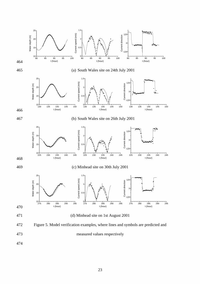
Comparisons between the model predictions and field measurements were made at all 208

of the sites where data were available, for both spring and neap tides. The degree of 209

agreement at the various sites was similar, so only the results at sites South Wales and 210

Minehead were presented herein. Field surveys at these two sites were carried out using 211

an Acoustic Doppler Current Profiler (ADCP) intermittently between 24/7/2001 and 212

1/8/2001. Figure 5 compares the model predictions with the four sets of observed 213

velocities and water depths. It can be seen that there is generally a good match in terms 214

of the period, phase and amplitude of the water depth and velocity variations for all sets 215

of results, even though the current speed and direction were sensitive to local 216

disturbances during measurement. In some flow direction graphs, the artefacts of the 217

flow suddenly switching direction by 180º should be ignored. This occurred when 218

velocity was close to zero, and therefore the flow direction was vulnerable to rounding 219

errors etc. The agreement was improved at some sites compared with previous studies 220

(Yang et al., 2008; Xia et al., 2010; Ahmadian et al., 2010). Therefore, the accuracy of 221

the model was deemed satisfactory, particularly considering the complexity of the tidal 222

flows in such a large domain. 223

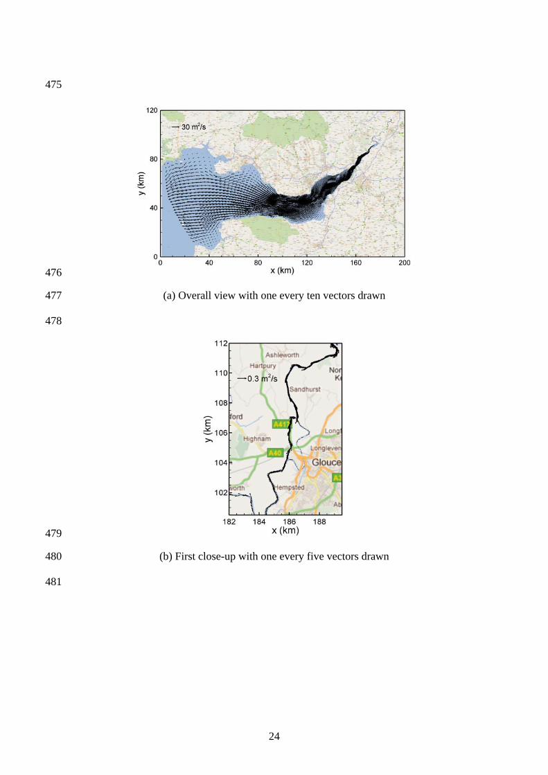
A snapshot of the predicted tidal current at the mean ebb tide is illustrated in Figure 6, 224

which highlights the disparate hydrodynamic scales captured by the model. In order to 225

simultaneously simulate the flow at the open sea near Lundy Island and the narrow 226

River Severn reaches near Apperley, there is a hundredfold difference between the sizes 227

of the largest and smallest grids. Because of the high density of the grid points, only 228

11

every tenth vector was drawn in Figure 6(a) to avoid clutter. As a result, the flow in the 229

River Severn can hardly be identified. In order to distinguish the individual velocity 230

vectors in the river, the overall flow field needs to be magnified multiple times. 231

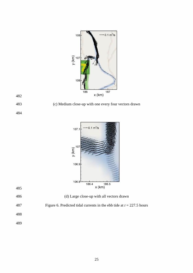
The instant of these graphical outputs was chosen when the tidal currents were 232

relatively strong. The predicted flow field in Figure 6 captured the ebb-tide feature in 233

the Bristol Channel, when water was flushing out of the basin. Corresponding to the 234

vast difference between the downstream and upstream widths, the unit-width discharges 235

also exhibit large variations, as is noted by the change in the magnitude of the reference 236

vectors in sub-figures. 237

238

5. Tidal response of Severn Estuary and Bristol Channel 239

After verifying the reliability of the hydrodynamic model, parametric studies were 240

undertaken to investigate the resonance characteristics of the Bristol Channel and 241

Severn Estuary. A simple thesis might first be put forward, which supposed that the 242

tidal range in the Severn Estuary was large because the tidal period of 12.42 hours 243

coincided with the resonant peak of the water body. This thesis was herein tested by 244

varying the tidal period at the seaward boundary and monitoring the water surfaces at 245

some monitoring points, which served as the virtual tidal gauge stations. This study 246

only examined the oscillations that had become repetitive after some spin-up period. 247

The monitoring points defined in Figure 7 were supposed to be representative of the 248

water surface variations over the whole region. In this study, 13 points spread over the 249

domain, among which P1 ~ P8 were located in the Bristol Channel and P9 ~ P13 were 250

within the Severn Estuary. They were also chosen to be close to some well-known 251

12

geographical sites, and the correspondence between them and the actual places are listed 252

in the first two columns of Table 1. 253

In modelling the tidal response, the computational condition was identical to that 254

used in the model verification, except the seaward boundary condition. In this pilot 255

investigation, the mean water level was held at 0 m, and the amplitude of the input 256

sinusoidal wave was maintained at 1 m, but the period of oscillation was varied. In total, 257

sixteen scenarios were run, with periods of 1, 2, 4, 5, 6, 7, 8, 9, 10, 11, 12, 16, 20, 24 258

and 28, respectively. 259

Some sample water surface variations at monitoring point P12 are shown in Figure 8, 260

which are the water level time series after the formation of stabilised oscillations. They 261

demonstrate how the water level oscillation at this location responds to the excitation at 262

the sea boundary of various frequencies. In order to easily distinguish the curves of 263

different periods, the results of neighbouring periods are plotted in two separate sub-264

figures. The response curves with periods of 1, 4, 8 and 16 hours are plotted in Figure 265

8(a), and those with periods of 2, 6, 12 and 24 hours in Figure 8(b). It is clear that the 266

wave amplitudes with periods of 1 and 24 hours are relatively small, and resonance 267

occurs at some intermediate period, which gives the maximum amplitude. 268

At each monitoring point under each excitation period, an amplification factor, 269

defined as the ratio between the wave height at the indicated location and that at the 270

open boundary, can be calculated from a curve similar to those shown in Figure 8. A 271

response curve for each monitoring point can then be constructed by plotting the 272

amplification factor versus the wave period. Figure 9 shows the response curves for all 273

the thirteen monitoring points, from which a major resonance peak at 8 hours is seen for 274

13

most parts of the basin. Therefore, it seems that the eight-hour tide is the first mode of 275

the basin, instead of the M2 tide with a period of 12.42 hours. 276

At short wave periods, e.g. less than 6 hours, the amplification factor varies 277

drastically, both with periods and among points. The amplification factor can also be 278

much less than unity at some points with very small tidal periods. At longer periods, e.g. 279

greater than 6 hours, the amplification factor continually increases in the order P1, 280

P2 …, until P12, which is generally in the direction towards the head of the basin. The 281

tidal ranges at these twelve sites reach their peaks at the same period of 8 hours. This 282

implies that the tide is most amplified over the inner part of the computational domain 283

in the Severn Estuary, which is consistent with the observations in real life. Monitoring 284

point P13 shows a distinctive trend, as its wave height is much smaller than that at P12, 285

and its resonance period shifts to 9 hours. This implies that the maximum tidal range 286

across the estuary occurs somewhere between P12 and P13, under the assumption of the 287

presently-used mean water level and tidal amplitude at the open boundary. Beyond the 288

resonance at 8-9 hours, the amplification factor gradually decreases with the further 289

increase of the wave period. 290

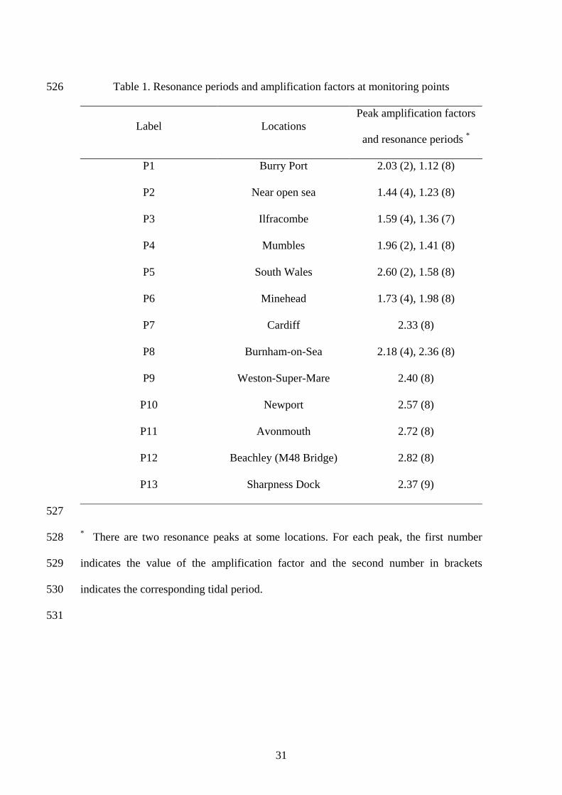
Although resonance is experienced by all of the points at around 8 hours, a double-291

peak structure appears in the amplification factor curves at some points located in the 292

outer domain. The local maximum amplification factors and the periods at which these 293

factors were recorded, as given in brackets, are listed in the third column of Table 1. 294

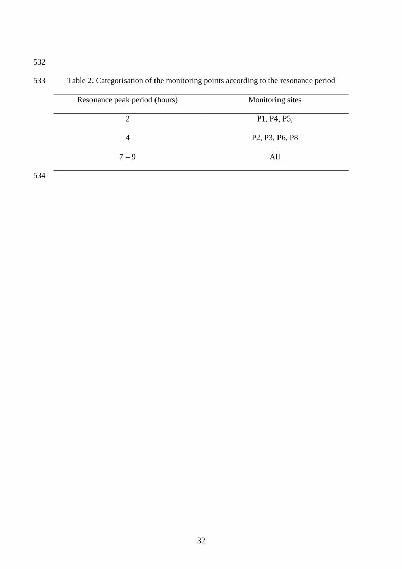
Table 2 classifies the monitoring points in terms of the resonance peak periods. It can 295

be seen from the tables that there are in fact several distinct resonance peaks in different 296

regions of the domain. Major resonance in the Bristol Channel occurs at periods shorter 297

than 8 hours. The north side of the Channel, where points P1, P4 and P5 reside, sees the 298

14

maximum tidal range occur at a period of 2 hours. On the south side of the Channel, P2, 299

P3, P6 and P8 experience resonance when the period is 4 hours. Whilst the overall first 300

mode of resonance seems to correspond to a universal period of around 8 hours across 301

the entire region, some regions in the Bristol Channel also experience significant, if not 302

greater, resonance when the wave frequency doubles or quadruples. 303

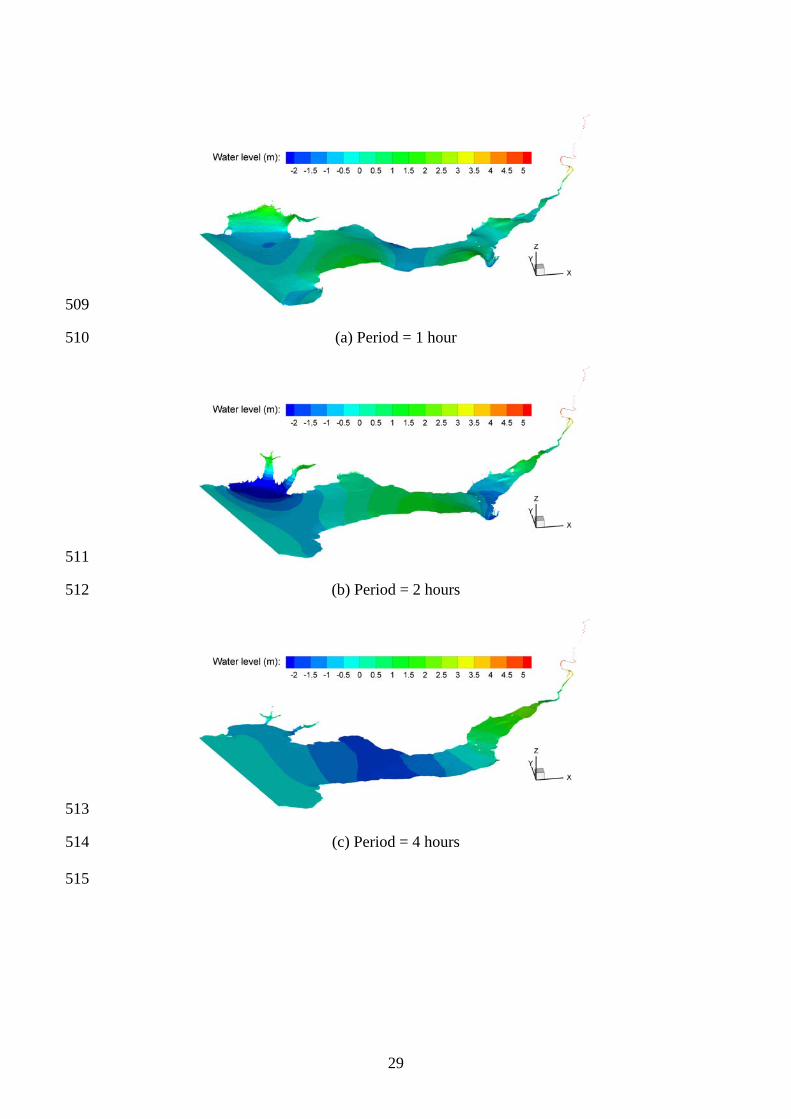
Figure 10 illustrates the three-dimensional water surface positions when the tide at 304

the seaward boundary is at the mid-flood phase. These graphs can be used to explain 305

how the tide is amplified inside the domain. At shorter wave periods, e.g. in the case of 306

Figure 10(a), water surface undulations can be clearly noticed, with the greenish-307

coloured contours separated by the bluish-coloured contours along the basin. The 308

interval of the separation continually reduces towards the upstream direction. At longer 309

wave periods, e.g. in the case of Figure 10(f), the water surface is almost flat across the 310

domain except in the upstream river reaches. The tide is less dynamic, and the 311

propagation towards the head of the basin cannot be clearly traced any more. 312

In the water surface plots, the greenish colour indicates the tidal wave crests, whilst 313

the bluish colour indicates wave troughs. The horizontal distance between them reflects 314

half the wave length. The longer tidal period leads to a longer tidal length, as 315

demonstrated in Figure 10. One main mechanism of resonance in this water body seems 316

to comply with the quarter-wavelength resonator theory, which states that the tidal 317

resonance is most striking when the length of the water basin is about a quarter of the 318

incident tidal wavelength. For a natural water basin with irregular geometry and 319

bathymetry, however, it is not easy to underpin exactly the length of the basin. Roughly 320

speaking, the characteristic length of the Severn Estuary and Bristol Channel is of the 321

same order of magnitude as the wavelength associated with a two-hour-period tidal 322

15

wave, as evident in Figure 10(b). By quadrupling the tidal period, the wavelength also 323

increases approximately fourfold. Hence, the characteristic length of the studied water 324

body is approximately equal to a quarter of the eight-hour tidal wavelength, which 325

corresponds well to the occurrence of maximum amplification factor at 8 hours 326

observed among most of the monitoring points shown in Figure 9. The above analyses 327

only give a gross picture of the tidal behaviour in the region, when the integrated water 328

body in the Bristol Channel and Severn Estuary is taken as a whole. Hence, the overall 329

resonance occurs at a period of around 8 hours in the central part of the estuary, e.g. 330

between P6 and P12, where the amplification factor is the greatest. The maximum 331

amplification factor decreases towards the open boundary and towards the tidal limit. 332

When examining some smaller semi-enclosed water bodies inside the studied domain, 333

e.g. the Carmarthen Bay, the resonant motions occur at smaller periods and wavelengths, 334

which explains some of the shorter resonance periods at some monitoring points 335

observed in Figure 9 and listed in Tables 1 and 2. 336

337

6. Conclusions 338

A high-quality curvilinear mesh was generated to cover the Bristol Channel, Severn 339

Estuary and downstream reach of the River Severn, which accommodates grid cells 340

with two orders of magnitude difference in size. The landward boundary was set 341

slightly upstream of the tidal limit close to Gloucester. The seaward boundary was set at 342

the downstream end of the Bristol Channel. Rigorous model verifications were 343

undertaken using field observations of tidal levels and currents. 344

Long-wave-induced hydrodynamic processes in the Severn Estuary and Bristol 345

Channel have been studied using the established model. The frequency response 346

16

characteristics of the water body were assessed when subjected to sinusoidal-wave 347

excitation at the open sea boundary. By normalising the predicted wave heights with 348

reference to the input wave height, the amplification factors were determined as a 349

function of the location and wave period. The consequent periods obtained for the first 350

mode of resonance across the whole region ranged from 8 to 9 hours. The 351

hydrodynamic processes in the Bristol Channel and Severn Estuary were highly 352

complex, owing to the large area, irregular land boundaries, complicated bathymetry, 353

and existence of extensive intertidal flats. In some small semi-enclosed bays in the 354

Bristol Channel, large water surface oscillations might be excited at periods no more 355

than 4 hours. The maximum tidal range was confirmed to occur in the upper part of the 356

Severn Estuary, where the input wave was amplified by up to three times. 357

It should be noted that this is a preliminary research. The maximum tidal range has 358

been found to occur between P12 and P13, which are two points rather far apart. More 359

monitoring points will be required to investigate the flow behaviour in a greater detail, 360

especially in the regions that have proved to be of interest in this paper. Further studies 361

are also being undertaken to relate the present type of analyses more closely to the real 362

tidal spectrum and to examine the Severn River bore. The present method can also be 363

used to examine the fundamental mode of resonance in harbours and bays in response to 364

the attack of long waves, such as tsunamis, which have periods from many minutes to 365

an hour and may cause unexpected damage. 366

367

Acknowledgements 368

We acknowledge the financial support from the State Key Laboratory of Ocean 369

Engineering, Shanghai Jiao Tong University (Grant No. GKZD010061), and from the 370

17

Open Research Fund Program of the State Key Laboratory of Water Resources and 371

Hydropower Engineering Science, Wuhan University (Grant No. 2011A005). 372

373

References 374

[1] Ahmadian R, Falconer R A, Lin B. (2010). Hydro-environmental modeling of the 375

proposed Severn barrage. Proceedings of the Institution of Civil Engineers, 376

Energy, 163 (3): 107-117 377

[2] Falconer RA, Xia J, Lin B, Ahmadian R. (2009). The Severn Barrage and other 378

tidal energy options: hydrodynamic and power output modelling. Science in 379

China Series E, Technological Sciences, 52 (11): 3105-3424 380

[3] Kirby R, and Shaw TL. (2005). Severn Barrage, UK – environmental reappraisal. 381

Proceedings of the Institution of Civil Engineers – Engineering Sustinability, 158: 382

31-39 383

[4] Liang D, Lin B and Falconer RA. (2007a). A boundary-fitted numerical model 384

for flood routing with shock-capturing capability. Journal of hydrology, 332: 385

477-486 386

[5] Liang D, Lin B and Falconer RA. (2007b). Simulation of rapidly varying flow 387

using an efficient TVD-MacCormack scheme. International journal for 388

numerical methods in fluids, 53:811-826 389

[6] Liang D, Wang X, Falconer RA and Bockelmann-Evans BN. (2010). Solving the 390

depth-integrated solute transport equation with a TVD-MacCormack scheme, 391

Environmental modelling & Software, 25:1619-1629 392

[7] Liang D, Xia J, Falconer RA and Zhang J. (2013). On the refinement of a 393

boundary-fitted shallow water model. Submitted to coastal engineering journal 394

18

[8] Marmer, H.A. (1922). Tides in the Bay of Fundy, Geographical Review, 12(2): 395

195-205. 396

[9] Pan CH, Lin BY, and Mao XZ. (2007). Case Study: Numerical Modeling of the 397

Tidal Bore on the Qiantang River, China. Journal of hydraulic engineer, 133(2): 398

130-138 399

[10] POL. (2004). POLPRED for Windows user guide. 62pp 400

[11] Proudman, J. (1953). Dynamical oceanography, Methuen-Wiley, London, 409 pp. 401

[12] Stapleton, C.M., Wyer, M.D., Kay, D., Bradford, M., Humphrey, N., Wilkinson, 402

J., Lin, B., Yang, Y., Falconer, R.A., Watkins, J., Francis, C.A., Crowther, J., 403

Paul,N.D., Jones, K. and McDonald, A.T., (2007). Fate and Transport of 404

Particles in Estuaries, Volume IV. Environment Agency Science Report 405

SC000002/SR2. 139pp 406

[13] Uncles RJ. (1981). A numerical simulation of the vertical and horizontal M2 tide 407

in the Bristol Channel and comparison with observed data. Limnology and 408

Oceanography, 26(3): 571-577 409

[14] Xia J, Falconer R A, Lin B. (2010a). Numerical model assessment of tidal stream 410

energy resources in the Severn Estuary, UK, Proceedings of the Institution of 411

Mechanical Engineers, Part A: Power and Energy , 224 (7): 969-983 412

[15] Xia J, Falconer RA, Lin B. (2010b). Hydrodynamic impact of a tidal barrage in 413

the Severn Estuary, UK, Renewable Energy , 35 (7): 1455-1468 414

[16] Xing, X.Y., J.J. Lee, and F. Raichlen. (2008). Comparison of computed basin 415

response at San Pedro Bay with long period wave records, Proceedings of ICCE 416

2008, Vol.2, 1223-1235. 417

19

[17] Yang L, Lin B, Falconer RA. (2008). Modelling enteric bacteria levels in coastal 418

and estuarine waters, Proceedings of the Institution of Civil Engineers, 419

Engineering and Computational Mechanics , 161(4): 179-186 420

421

20

List of Figures 422

Figure 1. Map of the studied area with computational mesh superimposed 423

Figure 2. Bathymetry of the Bristol Channel and Severn Estuary 424

Figure 3. Water elevations at seaward boundary in model verification 425

Figure 4. Locations of the verification sites 426

Figure 5. Model verification examples, where lines are predicted values and symbols are 427

measured values 428

Figure 6. Predicted tidal currents in the ebb tide at t = 227.5 hours 429

Figure 7. Locations of the monitoring points 430

Figure 8. Water elevation oscillations at Site P12 due to tides of different periods 431

Figure 9. Relationship between amplification factor and tidal period 432

Figure 10. Water surface positions at mean flood tide at seaward boundary 433

434

List of Tables 435

Table 1. Resonance periods and amplification factors at monitoring points 436

Table 2. Categorisation of the monitoring points according to the resonance period 437

438

439

440

441

21

442

(a) Overall view (b) Close-up view of the upstream part 443

Figure 1. Map of the studied area with computational mesh superimposed 444

445

446

447

(a) Overall domain (b) Close-up view of the upstream part 448

Figure 2. Bathymetry of the Bristol Channel and Severn Estuary 449

450

451

22

452

t (hour)

Wat

erle

vel(

m)

0 24 48 72 96 120 144 168 192 216 240 264 288 312 336-5

0

5

453

Figure 3. Water elevations at seaward boundary in model verification 454

455

456

457

458

Figure 4. Locations of the verification sites 459

460

461

462

463

23

t (hour)

Wat

erd

epth

(m)

80 85 90 95 10010

15

20

25

t (hour)

Cu

rren

tsp

eed

(m/s

)

80 85 90 95 1000

0.5

1

1.5

t (hour)

Cu

rren

tdir

ectio

n

80 85 90 95 100

-120

0

120

464

(a) South Wales site on 24th July 2001 465

t (hour)

Wat

erd

epth

(m)

130 135 140 145 15010

15

20

25

t (hour)

Cu

rren

tsp

eed

(m/s

)

130 135 140 145 1500

0.5

1

1.5

t (hour)

Cu

rren

tdir

ectio

n

130 135 140 145 150

-120

0

120

466

(b) South Wales site on 26th July 2001 467

t (hour)

Wat

erd

epth

(m)

225 230 235 240 24510

15

20

25

t (hour)

Cu

rren

tsp

eed

(m/s

)

225 230 235 240 2450

0.5

1

1.5

t (hour)

Cu

rren

tdir

ectio

n

225 230 235 240 245

-120

0

120

468

(c) Minhead site on 30th July 2001 469

t (hour)

Wat

erd

epth

(m)

275 280 285 290 29510

15

20

25

t (hour)

Cu

rren

tsp

eed

(m/s

)

275 280 285 290 2950

0.5

1

1.5

t (hour)

Cur

rent

dir

ectio

n

275 280 285 290 295

-120

0

120

470

(d) Minhead site on 1st August 2001 471

Figure 5. Model verification examples, where lines and symbols are predicted and 472

measured values respectively 473

474

24

475

476

(a) Overall view with one every ten vectors drawn 477

478

479

(b) First close-up with one every five vectors drawn 480

481

25

482

(c) Medium close-up with one every four vectors drawn 483

484

485

(d) Large close-up with all vectors drawn 486

Figure 6. Predicted tidal currents in the ebb tide at t = 227.5 hours 487

488

489

26

490

491

Figure 7. Locations of the monitoring points 492

493

494

27

495

t (hour)

Wat

erle

vel(

m)

36 42 48 54 60-3

-1.5

0

1.5

3

T = 1 hour

T = 4 hours

T = 8 hours

T = 16 hours

496

(a) Period = 1, 4, 8 or 16 hours 497

498

t (hour)

Wat

erle

vel(

m)

36 42 48 54 60-3

-1.5

0

1.5

3

T = 2 hours

T = 6 hours

T = 12 hours

T = 24 hours

499

(b) Period = 2, 6, 12 or 24 hours 500

Figure 8. Water elevation oscillations at Site P12 due to tides of different periods 501

502

503

28

504

1

1

1

11

1 1 1 1 1 11 1 1 1

2

2

2

22 2 2 2

22 2

2 2 2 2

3

3

3

33 3 3 3

33

3

3 3 3 3

4

4

4

44

44 4

44

4

44 4 4

5

5 5

55

55 5

5

55

55 5 5

6

6

66

6

66

6

6

6

6

6

66

6

7

7

7

7

7

77

7

7

7

7

7

77

7

8

8

88

8

8 8

8

8

8

8

8

88

8

9

9

99

9

9 9

9

9

9

9

9

99

9

X

X

XX

X

X X

X

X

X

X

X

XX

X

A

A

A

A

A

AA

A

A

A

A

A

AA

A

B

B

B

B

B

BB

B

B

B

B

B

BB

B

C

C

C

C

C

C

CC C

CC

C

CC

C

Period (hours)

Am

plif

ica

tion

Fa

cto

r

0 4 8 12 16 20 24 280

1

2

3P1P2P3P4P5P6P7P8P9P10P11P12P13

1

2

3

4

5

6

7

8

9

X

A

B

C

505

Figure 9. Relationship between amplification factor and tidal period 506

507

508

29

509

(a) Period = 1 hour 510

511

(b) Period = 2 hours 512

513

(c) Period = 4 hours 514

515

30

516

(d) Period = 8 hours 517

518

(e) Period = 12 hours 519

520

(f) Period = 28 hours 521

Figure 10. Water surface positions at mean flood tide at seaward boundary 522

523

524

525

31

Table 1. Resonance periods and amplification factors at monitoring points 526

Label Locations Peak amplification factors

and resonance periods *

P1 Burry Port 2.03 (2), 1.12 (8)

P2 Near open sea 1.44 (4), 1.23 (8)

P3 Ilfracombe 1.59 (4), 1.36 (7)

P4 Mumbles 1.96 (2), 1.41 (8)

P5 South Wales 2.60 (2), 1.58 (8)

P6 Minehead 1.73 (4), 1.98 (8)

P7 Cardiff 2.33 (8)

P8 Burnham-on-Sea 2.18 (4), 2.36 (8)

P9 Weston-Super-Mare 2.40 (8)

P10 Newport 2.57 (8)

P11 Avonmouth 2.72 (8)

P12 Beachley (M48 Bridge) 2.82 (8)

P13 Sharpness Dock 2.37 (9)

527

* There are two resonance peaks at some locations. For each peak, the first number 528

indicates the value of the amplification factor and the second number in brackets 529

indicates the corresponding tidal period. 530

531

32

532

Table 2. Categorisation of the monitoring points according to the resonance period 533

Resonance peak period (hours) Monitoring sites

2 P1, P4, P5,

4 P2, P3, P6, P8

7 – 9 All

534