A dissertation submitted for the degree of Doctor of Philosophy Study on Soil-Screw Interaction of Exploration Robot for Surface and Subsurface Locomotion in Soft Terrain February 2011 by Kenji Nagaoka Department of Space and Astronautical Science School of Physical Sciences The Graduate University for Advanced Studies (Sokendai) JAPAN

Welcome message from author
This document is posted to help you gain knowledge. Please leave a comment to let me know what you think about it! Share it to your friends and learn new things together.
Transcript
A dissertation submitted for the degree of Doctor of Philosophy
Study on Soil-Screw Interaction of Exploration Robot
for Surface and Subsurface Locomotion in Soft Terrain
February 2011
by
Kenji Nagaoka
Department of Space and Astronautical Science
School of Physical Sciences
The Graduate University for Advanced Studies (Sokendai)
JAPAN

Acknowledgment
At completing this dissertation, I would like to extend my gratitude to all the people regarding
my research activity over the past five years.
Above all, I would like to express my deepest gratitude for my PI, Professor Takashi Kubota.
He has always encouraged me to aspire for getting my doctoral degree during research life at the
ISAS. I could pursue my studies and enhance my humanity under his distinguished direction.
Words cannot describe my gratitude for him.
I would also like to extend my sincere gratitude to my supervisor, Professor Satoshi Tanaka.
His suggestions and scientific knowledge brought a different perspective to my research.
I wish to express my gratitude for Professor Ichiro Nakatani, Professor Tatsuaki Hashimoto,
Professor Tetsuo Yoshimitsu, Professor Shin-ichiro Sakai, Professor Nobutaka Bando, Professor
Masatsugu Otsuki, Dr. Andrew Klesh and Dr. Genya Ishigami. Through my seminar presenta-
tions or individual discussions, their valuable suggestions enabled to cultivate my research. In
particular, Professor Otsuki helped me conduct various experiments, and he gave me numerous
advices in this five years. Without his continual support, I could not complete my dissertation.
I would like to sincerely appreciate Ms. Mayumi Oda, the secretary of the Kubota lab. Her
helps allowed me to do my research smoothly. Also, I wish to give my special thanks to my
labmates and great alumnae/alumni. Life in the lab with them were very precious to me, and I
thank them for having such productive days.
I acknowledge for Shimizu-Kikai, especially President Hideki Yamazaki. His supports and
advices enabled me to accomplish this study.
I greatly appreciate Mr. Eijiro Hirohama and Ms. Takemi Chiku, the stuff of the JAXA Space
Education Center in 2008. Thanks to their graceful supports, I had participated the NASA
Academy 2008 at the NASA Goddard Space Flight Center. That summer was definitely a very
pleasurable time for me, and I could lean and experience countless things during the project.
I also express my appreciation all the members of the ISAS football club. The daily exercise
with them gives momentary happiness to my hectic life.
Last of all, I am deeply grateful for my parents, Yoshiaki and Junko.
January 31, 2011
Kenji Nagaoka

Abstract
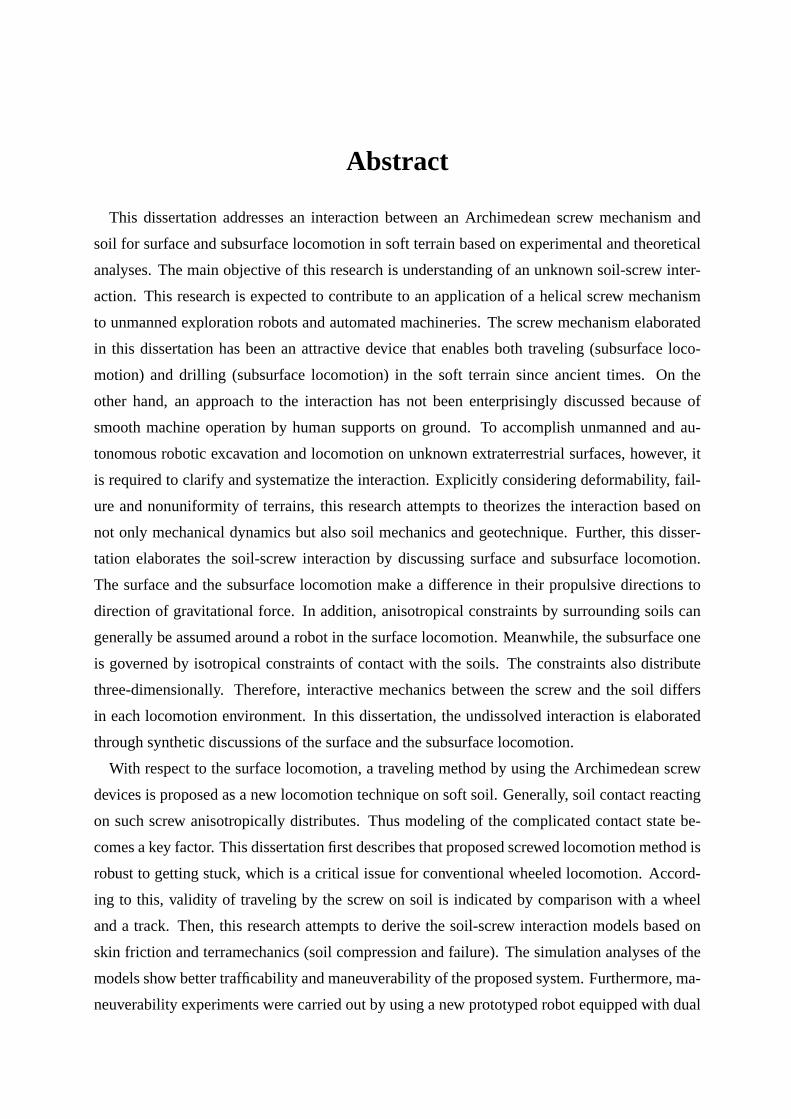
This dissertation addresses an interaction between an Archimedean screw mechanism and
soil for surface and subsurface locomotion in soft terrain based on experimental and theoretical
analyses. The main objective of this research is understanding of an unknown soil-screw inter-
action. This research is expected to contribute to an application of a helical screw mechanism
to unmanned exploration robots and automated machineries. The screw mechanism elaborated
in this dissertation has been an attractive device that enables both traveling (subsurface loco-
motion) and drilling (subsurface locomotion) in the soft terrain since ancient times. On the
other hand, an approach to the interaction has not been enterprisingly discussed because of
smooth machine operation by human supports on ground. To accomplish unmanned and au-
tonomous robotic excavation and locomotion on unknown extraterrestrial surfaces, however, it
is required to clarify and systematize the interaction. Explicitly considering deformability, fail-
ure and nonuniformity of terrains, this research attempts to theorizes the interaction based on
not only mechanical dynamics but also soil mechanics and geotechnique. Further, this disser-
tation elaborates the soil-screw interaction by discussing surface and subsurface locomotion.
The surface and the subsurface locomotion make a difference in their propulsive directions to
direction of gravitational force. In addition, anisotropical constraints by surrounding soils can
generally be assumed around a robot in the surface locomotion. Meanwhile, the subsurface one
is governed by isotropical constraints of contact with the soils. The constraints also distribute
three-dimensionally. Therefore, interactive mechanics between the screw and the soil differs
in each locomotion environment. In this dissertation, the undissolved interaction is elaborated
through synthetic discussions of the surface and the subsurface locomotion.
With respect to the surface locomotion, a traveling method by using the Archimedean screw
devices is proposed as a new locomotion technique on soft soil. Generally, soil contact reacting
on such screw anisotropically distributes. Thus modeling of the complicated contact state be-
comes a key factor. This dissertation first describes that proposed screwed locomotion method is
robust to getting stuck, which is a critical issue for conventional wheeled locomotion. Accord-
ing to this, validity of traveling by the screw on soil is indicated by comparison with a wheel
and a track. Then, this research attempts to derive the soil-screw interaction models based on
skin friction and terramechanics (soil compression and failure). The simulation analyses of the
models show better trafficability and maneuverability of the proposed system. Furthermore, ma-
neuverability experiments were carried out by using a new prototyped robot equipped with dual
Archimedean screw units on sand. Through the laboratory tests, it is confirmed that various
maneuvers can be achieved by changing rotational speed of each screw. Summarizing the re-
sulted maneuvers, directions of propulsive force that the prototyped robot exerts are presented.
In addition to these tests, trafficability tests of a single screw unit were conducted in sandy ter-
rain to comprehend its characteristics of drawbar pull and slip. The experimental results provide
qualitative analyses of the drawbar pull, and thereby the interaction can be discussed. Based
upon these considerations, this dissertation indicates applicability and feasibility of the screw
mechanism for the surface locomotion on the soft terrain.
With respect to the subsurface locomotion, this dissertation proposes a subsurface drilling
robot using the Archimedean screw mechanism. Prior to detailed discussion of the interaction,
this dissertation describes an advantage of a subsurface explorer. Moreover, this research qual-
itatively organizes how a robot achieve drilling motion in complicated subsurface environment.
In accordance with this remark, this dissertation indicates effectiveness of the screw mechanism
for the subsurface drilling. Then, a novel interaction model between the screw and the surround-
ing soils is proposed based on soil mechanism with screw geometry. In the interaction modeling,
by applying cavity expansion theory, the proposed model includes an increase of soil pressure
caused by laterally compressing subsoil. The validity of the model is discussed through experi-
mental analyses. Consequently, the model enables to calculate required torque of the screw with
depth. The result is expected to lead not only to understanding of the interaction but also to de-
sign optimization of screw geometry. Furthermore, an effective screw mechanism (Contra-rotor
Screw Drilling mechanism) is proposed to achieve an efficient self-drilling. The new mechanism
is experimentally investigated, and thereby its feasibility and proper conditions are indicated.
In this dissertation, the unknown soil-screw interaction of the Archimedean screw mechanism
in the soft terrain is addressed from the standpoints of the surface and the subsurface locomotion.
So far, studies on theoretical approaches of the practical application of such screw mechanism
have been particularly limited although it is an interesting and useful tool for the locomotion.
Therefore, this research is expected to provide an initiative of the screw mechanism. This re-
search fosters the understanding of the complicated soil-screw interaction by discussing the
applications in the surface and subsurface locomotion. Additionally, this dissertation makes a
significant contribution in the field of general screw mechanism and leads to the design optimiza-
tion and the motion control. The developed ideas can cover applications of manned/unmanned
activities on Earth.
Contents
Chapter 1. Introduction 1
1.1 Background . . . . . . . . . . . . . . . . . . . . . . . . . . . . . . . . . . . 1
1.2 Motivation . . . . . . . . . . . . . . . . . . . . . . . . . . . . . . . . . . . . 3
1.2.1 Requirements for Space Robotics. . . . . . . . . . . . . . . . . . . . 3
1.2.2 Applicability of Archimedean Screw Mechanism. . . . . . . . . . . . 3
1.3 Purpose and Approach. . . . . . . . . . . . . . . . . . . . . . . . . . . . . . 4
1.4 Research Contributions. . . . . . . . . . . . . . . . . . . . . . . . . . . . . . 6
1.5 Outline . . . . . . . . . . . . . . . . . . . . . . . . . . . . . . . . . . . . . . 6
Chapter 2. Archimedean Screw Mechanism 11
2.1 Geometric Modeling of Screw Mechanism. . . . . . . . . . . . . . . . . . . . 11
2.1.1 Screw Slope Parameter. . . . . . . . . . . . . . . . . . . . . . . . . . 12
2.1.2 Screw Pitch . . . . . . . . . . . . . . . . . . . . . . . . . . . . . . . 13
2.1.3 Screw Surface Area. . . . . . . . . . . . . . . . . . . . . . . . . . . 14
2.1.4 Slip . . . . . . . . . . . . . . . . . . . . . . . . . . . . . . . . . . . 14
2.2 Related Works. . . . . . . . . . . . . . . . . . . . . . . . . . . . . . . . . . 14
2.2.1 Historical Background of Screw Vehicles. . . . . . . . . . . . . . . . 14
2.2.2 Historical Background of Screw Drilling. . . . . . . . . . . . . . . . . 17
2.3 Summary. . . . . . . . . . . . . . . . . . . . . . . . . . . . . . . . . . . . . 18
Chapter 3. Modeling of Screw Surface Locomotion 19
3.1 Challenge Statement for Robotic Surface Locomotion. . . . . . . . . . . . . . 19
3.2 Principle of Fundamental Surface Locomotion. . . . . . . . . . . . . . . . . . 22
3.3 Proposal of Screw Drive Rover System. . . . . . . . . . . . . . . . . . . . . 23
3.4 Mobility Analysis based on Conventional Ideas. . . . . . . . . . . . . . . . . 26
3.4.1 Skin Friction Model . . . . . . . . . . . . . . . . . . . . . . . . . . . 26
3.4.2 Simulation Analysis based on Skin Friction Model. . . . . . . . . . . 29
3.4.3 Terramechanics Model. . . . . . . . . . . . . . . . . . . . . . . . . . 32
- i -
Contents
3.4.4 Simulation Analysis based on Terramechanics Model. . . . . . . . . . 41
3.5 Synthetic Modeling of Soil-Screw Interaction. . . . . . . . . . . . . . . . . . 45
3.5.1 A Lesson for Synthetic Interaction Model. . . . . . . . . . . . . . . . 45
3.5.2 Dynamics Modeling. . . . . . . . . . . . . . . . . . . . . . . . . . . 46
3.5.3 Simulation Analysis. . . . . . . . . . . . . . . . . . . . . . . . . . . 49
3.6 Summary. . . . . . . . . . . . . . . . . . . . . . . . . . . . . . . . . . . . . 49
Chapter 4. Experimental Characteristics of Screw Surface Locomotion 51
4.1 Trafficability Tests of Archimedean Screw Unit. . . . . . . . . . . . . . . . . 51
4.1.1 Laboratory Test Environment. . . . . . . . . . . . . . . . . . . . . . 51
4.1.2 Evaluation Scheme. . . . . . . . . . . . . . . . . . . . . . . . . . . . 51
4.1.3 Results and Discussion. . . . . . . . . . . . . . . . . . . . . . . . . . 55
4.2 Comparative Analysis of Experimental and Theoretical Trafficability. . . . . . 60
4.3 Empirical Maneuverability of Screw Drive Rover System on Sand. . . . . . . . 63
4.3.1 Experimental Setup. . . . . . . . . . . . . . . . . . . . . . . . . . . 63
4.3.2 Fundamental Characteristics of Forward Traveling. . . . . . . . . . . . 63
4.3.3 Classification of Empirical Maneuvers. . . . . . . . . . . . . . . . . . 64
4.3.4 Maneuverability Analysis. . . . . . . . . . . . . . . . . . . . . . . . 65
4.4 Adaptability to Climbing Rocks. . . . . . . . . . . . . . . . . . . . . . . . . 68
4.5 Summary. . . . . . . . . . . . . . . . . . . . . . . . . . . . . . . . . . . . . 69
Chapter 5. Modeling and Analysis of Screw Subsurface Locomotion 71
5.1 Expectation for Lunar Subsurface Exploration. . . . . . . . . . . . . . . . . . 71
5.2 Related Works and Challenge of Subsurface Explorer. . . . . . . . . . . . . . 74
5.3 Robotic Subsurface Explorer. . . . . . . . . . . . . . . . . . . . . . . . . . . 77
5.3.1 Robotic Locomotion in Soil. . . . . . . . . . . . . . . . . . . . . . . 77
5.3.2 Synopsis of Robotic Subsurface Explorer System. . . . . . . . . . . . 78
5.3.3 Subsurface Locomotion Principle. . . . . . . . . . . . . . . . . . . . 78
5.4 Fundamental Drilling Performance of SSD Unit. . . . . . . . . . . . . . . . . 85
5.5 Mathematical Modeling of Screw Drilling. . . . . . . . . . . . . . . . . . . . 87
5.5.1 Dynamics Modeling. . . . . . . . . . . . . . . . . . . . . . . . . . . 87
5.5.2 Cavity Expansion Theory. . . . . . . . . . . . . . . . . . . . . . . . 92
5.5.3 Parametric Analysis. . . . . . . . . . . . . . . . . . . . . . . . . . . 95
5.6 Experimental Evaluation. . . . . . . . . . . . . . . . . . . . . . . . . . . . . 95
5.6.1 Experimental Methodology. . . . . . . . . . . . . . . . . . . . . . . 95
- ii -
Contents
5.6.2 Results and Discussions. . . . . . . . . . . . . . . . . . . . . . . . . 97
5.7 Summary. . . . . . . . . . . . . . . . . . . . . . . . . . . . . . . . . . . . . 100
Chapter 6. Proposal of Effective Screw Drilling Mechanism 101
6.1 Proposal of Non-Reaction Screw Mechanism: CSD. . . . . . . . . . . . . . . 101
6.2 Evaluation Indexes for Experimental Analysis. . . . . . . . . . . . . . . . . . 103
6.2.1 Drilling Performance. . . . . . . . . . . . . . . . . . . . . . . . . . . 103
6.2.2 Equivalent Angular Velocity and Rotational Ratio. . . . . . . . . . . . 104
6.3 Experimental Analyses. . . . . . . . . . . . . . . . . . . . . . . . . . . . . . 104
6.3.1 Overview . . . . . . . . . . . . . . . . . . . . . . . . . . . . . . . . 104
6.3.2 Verification of Penetration with Non-Reaction. . . . . . . . . . . . . . 106
6.3.3 Performance Evaluation Based on Kinetic Driving States. . . . . . . . 106
6.3.4 Performance Evaluation Based on Dynamic Inputs. . . . . . . . . . . 108
6.4 Proposal of Screw Subsurface Explorer. . . . . . . . . . . . . . . . . . . . . 110
6.5 Simulation Case Study: A Guideline for Design. . . . . . . . . . . . . . . . . 114
6.6 Summary. . . . . . . . . . . . . . . . . . . . . . . . . . . . . . . . . . . . . 115
Chapter 7. Conclusions 117
7.1 Concluding Remarks. . . . . . . . . . . . . . . . . . . . . . . . . . . . . . . 117
7.2 Future Works. . . . . . . . . . . . . . . . . . . . . . . . . . . . . . . . . . . 119
Appendix A Moving Direction Control based on Skin Friction Model 121
A.1 Control System. . . . . . . . . . . . . . . . . . . . . . . . . . . . . . . . . . 121
A.2 Pilot Scheme of Control Law. . . . . . . . . . . . . . . . . . . . . . . . . . . 123
A.3 Simulation Case Study. . . . . . . . . . . . . . . . . . . . . . . . . . . . . . 123
Appendix B Tractive Limitations of Rigid Wheels on Soil 125
B.1 Identifying Current Situation. . . . . . . . . . . . . . . . . . . . . . . . . . . 125
B.2 Terramechanics Model of a Rigid Wheel. . . . . . . . . . . . . . . . . . . . . 126
B.3 Parametric Analysis based on Terramechanics Model. . . . . . . . . . . . . . 129
B.3.1 Fundamental Simulation Conditions. . . . . . . . . . . . . . . . . . . 129
B.3.2 Results and Discussions. . . . . . . . . . . . . . . . . . . . . . . . . 130
B.4 Compliance of Interaction Model with Single Wheel Test. . . . . . . . . . . . 136
B.4.1 Apparatus of Conventional Single Wheel Test. . . . . . . . . . . . . . 136
B.4.2 Key Suggestion of Test Outcomes and Their Implications. . . . . . . . 136
B.5 Summary. . . . . . . . . . . . . . . . . . . . . . . . . . . . . . . . . . . . . 137
- iii -
Contents
Appendix C Comparative Vehicle Model 139
C.1 Wheeled Vehicle Model. . . . . . . . . . . . . . . . . . . . . . . . . . . . . 139
C.2 Tracked Vehicle Model. . . . . . . . . . . . . . . . . . . . . . . . . . . . . . 139
Appendix D Penetration Equation 141
Bibliography 143
Publications 159
- iv -
List of Figures
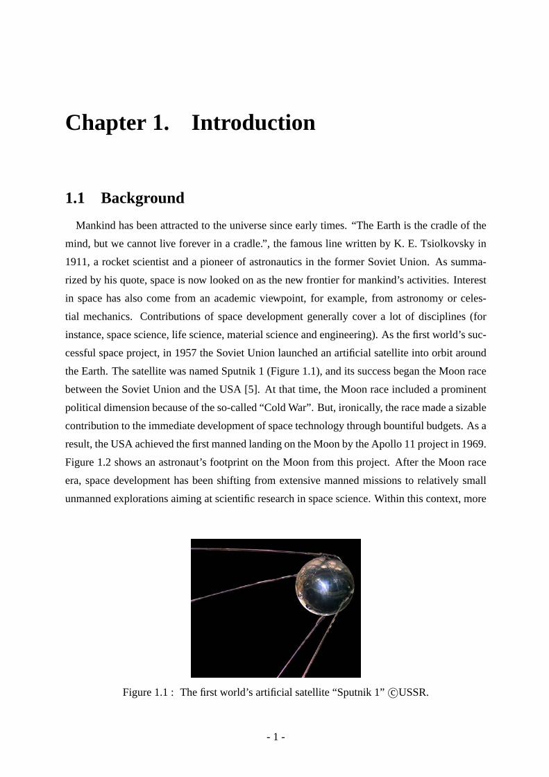
1.1 The first world’s artificial satellite “Sputnik 1”c©USSR . . . . . . . . . 1
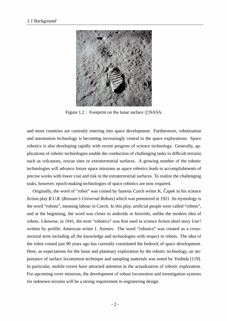
1.2 Footprint on the lunar surfacec©NASA . . . . . . . . . . . . . . . . . 2
1.3(a) Archimedean screw pump [50]. . . . . . . . . . . . . . . . . . . . . . 5
1.3(b) Earth auger machinec©Hokuriku Eletec Co., Ltd.. . . . . . . . . . . . 5
1.3(c) Screw pilesc©Apollo Piling Systems . . . . . . . . . . . . . . . . . . 5
1.3(d) Marsh Screw Amphibian [45]. . . . . . . . . . . . . . . . . . . . . . 5
1.3 Practical applications of the Archimedean screw mechanism. . . . . . 5
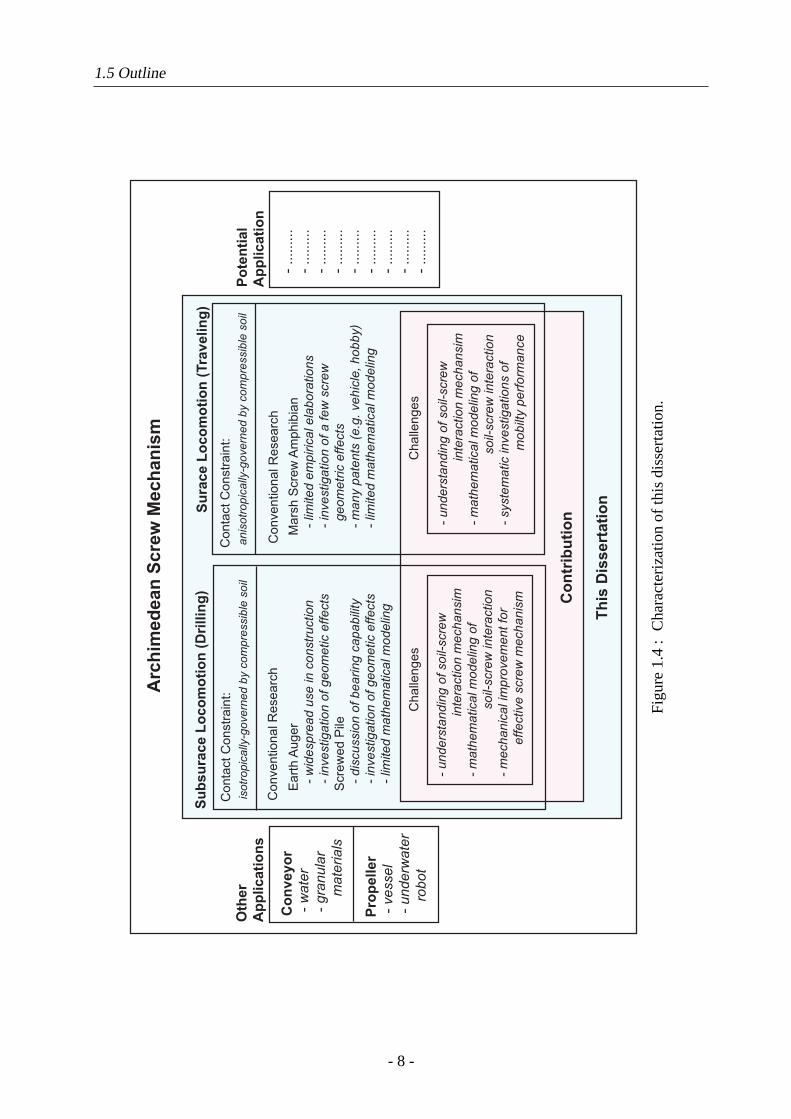
1.4 Characterization of this dissertation. . . . . . . . . . . . . . . . . . . 8
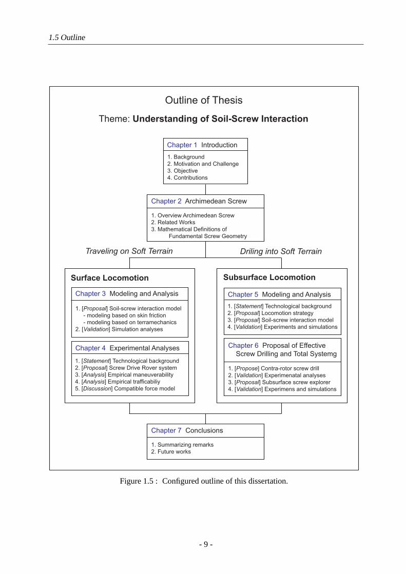
1.5 Configured outline of this dissertation. . . . . . . . . . . . . . . . . . 9
2.1(a) Logarithmic helix . . . . . . . . . . . . . . . . . . . . . . . . . . . . 12
2.1(b) Cylindrical helix . . . . . . . . . . . . . . . . . . . . . . . . . . . . . 12
2.1 Geometric models of screw helices. . . . . . . . . . . . . . . . . . . 12
2.2(a) Cylindrical helix. . . . . . . . . . . . . . . . . . . . . . . . . . . . . 13
2.2(b) Logarithmic helix . . . . . . . . . . . . . . . . . . . . . . . . . . . . 13
2.2 Mathematical drawing of screw helices. . . . . . . . . . . . . . . . . 13
2.3(a) Relationship betweena andη . . . . . . . . . . . . . . . . . . . . . . 15
2.3(b) Relationship between∆Asc/∆θ andη . . . . . . . . . . . . . . . . . . 15
2.3(c) Relationship betweenp andθ . . . . . . . . . . . . . . . . . . . . . . 15
2.3 Functional behaviors of logarithmic screw geometry. . . . . . . . . . . 15
2.4(a) Patent by Wells [34]. . . . . . . . . . . . . . . . . . . . . . . . . . . 16
2.4(b) Patent by Code [37]. . . . . . . . . . . . . . . . . . . . . . . . . . . 16
2.4(c) Marsh screw amphibian [40]. . . . . . . . . . . . . . . . . . . . . . . 16
2.4 Various types of marsh screw amphibians. . . . . . . . . . . . . . . . 16
3.1(a) Lunokhod 1c©Lavochkin Association. . . . . . . . . . . . . . . . . . 21
3.1(b) PROP-M roverc©VNII Transmash. . . . . . . . . . . . . . . . . . . . 21
3.1(c) Sojournerc©NASA/JPL . . . . . . . . . . . . . . . . . . . . . . . . . 21
- v -
List of Figures
3.1(d) MER c©NASA/JPL . . . . . . . . . . . . . . . . . . . . . . . . . . . 21
3.1(e) PROP-F rover [11]. . . . . . . . . . . . . . . . . . . . . . . . . . . . 21
3.1(f) MINERVA c©JAXA/ISAS . . . . . . . . . . . . . . . . . . . . . . . . 21
3.1 Space exploration rovers launched in past and current missions. . . . . 21
3.2(a) Indoor experimentation. . . . . . . . . . . . . . . . . . . . . . . . . 21
3.2(b) Computer simulation. . . . . . . . . . . . . . . . . . . . . . . . . . . 21
3.2 Trial-and-error approach for extricating the stuck Spirit roverc©NASA/JPL 21
3.3(a) Friction against ground. . . . . . . . . . . . . . . . . . . . . . . . . 22
3.3(b) External contact. . . . . . . . . . . . . . . . . . . . . . . . . . . . . 22
3.3(c) Additional thruster. . . . . . . . . . . . . . . . . . . . . . . . . . . . 22
3.3 Method of propulsive force for locomotion on rigid ground. . . . . . . 22
3.4(a) 3D CAD drawing . . . . . . . . . . . . . . . . . . . . . . . . . . . . 24
3.4(b) Prototype overview . . . . . . . . . . . . . . . . . . . . . . . . . . . 24
3.4 Schematic of Screw Drive Rover system. . . . . . . . . . . . . . . . . 24
3.5(a) Internal structure of main body and hinge legs. . . . . . . . . . . . . . 25
3.5(b) Cross-section diagram of screw drive unit. . . . . . . . . . . . . . . . 25
3.5 Mechanical structure of Screw Drive Rover. . . . . . . . . . . . . . . 25
3.6 Illustration of moving hinge legs (front view). . . . . . . . . . . . . . 26
3.7 Simplified dynamics model of Screw Drive Rover. . . . . . . . . . . . 28
3.8(a) Case 1. . . . . . . . . . . . . . . . . . . . . . . . . . . . . . . . . . 29
3.8(b) Case 2. . . . . . . . . . . . . . . . . . . . . . . . . . . . . . . . . . 29
3.8(c) Case 3. . . . . . . . . . . . . . . . . . . . . . . . . . . . . . . . . . 29
3.8(d) Case 4. . . . . . . . . . . . . . . . . . . . . . . . . . . . . . . . . . 29
3.8(e) Case 5. . . . . . . . . . . . . . . . . . . . . . . . . . . . . . . . . . 29
3.8(f) Case 6 . . . . . . . . . . . . . . . . . . . . . . . . . . . . . . . . . . 29
3.8(g) Case 7. . . . . . . . . . . . . . . . . . . . . . . . . . . . . . . . . . 29
3.8(h) Case 8. . . . . . . . . . . . . . . . . . . . . . . . . . . . . . . . . . 29
3.8 Simulation results: Dynamic trajectories of the Screw Drive Rover model29
3.9(a) Fr with resistances. . . . . . . . . . . . . . . . . . . . . . . . . . . . 30
3.9(b) k1 with resistances. . . . . . . . . . . . . . . . . . . . . . . . . . . . 30
3.9(c) ωr andωl with resistances. . . . . . . . . . . . . . . . . . . . . . . . 30
3.9(d) 3D plots of accelerations with resistances. . . . . . . . . . . . . . . . 30
3.9(e) 2D plots of accelerations with resistances. . . . . . . . . . . . . . . . 30
3.9(f) 3D plots of accelerations without resistances. . . . . . . . . . . . . . . 30
3.9(g) 2D plots of accelerations without resistances. . . . . . . . . . . . . . . 30
- vi -
List of Figures
3.9 Simulated distribution of parameters and generated accelerations with
η = 30deg . . . . . . . . . . . . . . . . . . . . . . . . . . . . . . . . 30
3.10(a) 3D plots atη = 15deg . . . . . . . . . . . . . . . . . . . . . . . . . . 31
3.10(b) 2D plots atη = 15deg . . . . . . . . . . . . . . . . . . . . . . . . . . 31
3.10(c) 3D plots atη = 45deg . . . . . . . . . . . . . . . . . . . . . . . . . . 31
3.10(d) 2D plots atη = 45deg . . . . . . . . . . . . . . . . . . . . . . . . . . 31
3.10(e) 3D plots atη = 75deg . . . . . . . . . . . . . . . . . . . . . . . . . . 31
3.10(f) 2D plots atη = 75deg . . . . . . . . . . . . . . . . . . . . . . . . . . 31
3.10 Simulated distribution of accelerations without frictional resistances:
variousη . . . . . . . . . . . . . . . . . . . . . . . . . . . . . . . . . 31
3.11(a) 3D data atk2 = 0.5 . . . . . . . . . . . . . . . . . . . . . . . . . . . . 32
3.11(b) 2D data atk2 = 0.5 . . . . . . . . . . . . . . . . . . . . . . . . . . . . 32
3.11(c) 3D data atk2 = 2 . . . . . . . . . . . . . . . . . . . . . . . . . . . . . 32
3.11(d) 2D data atk2 = 2 . . . . . . . . . . . . . . . . . . . . . . . . . . . . . 32
3.11 Simulated distribution of accelerations without frictional resistances:
η = 30deg and variousk2 . . . . . . . . . . . . . . . . . . . . . . . . 32
3.12 Kinematics model of the screw unit. . . . . . . . . . . . . . . . . . . 34
3.13 Soil-screw interaction model. . . . . . . . . . . . . . . . . . . . . . . 35
3.14 Relationship betweenθs f andh/R0 . . . . . . . . . . . . . . . . . . . 35
3.15(a) Trajectories of screw flight and soil displacement. . . . . . . . . . . . 37
3.15(b) Soil shearing ellipse. . . . . . . . . . . . . . . . . . . . . . . . . . . 37
3.15 Elliptic trajectory of soil shearing. . . . . . . . . . . . . . . . . . . . 37
3.16(a) Illustration of effective shearing distance. . . . . . . . . . . . . . . . 38
3.16(b) Parametric analysis ofds depending onη . . . . . . . . . . . . . . . . 38
3.16 Effective distance of soil shearing. . . . . . . . . . . . . . . . . . . . 38
3.17 Motion resistance by bulldozing soil. . . . . . . . . . . . . . . . . . . 40
3.18 Simulation plots ofFBx andhB . . . . . . . . . . . . . . . . . . . . . . 40
3.19 Angle components of stresses for drawbar pull on circular and elliptic
surfaces along angles. . . . . . . . . . . . . . . . . . . . . . . . . . 42
3.20(a) With varyingη , c3 = 0.2 andc4 = 0.03 . . . . . . . . . . . . . . . . . 44
3.20(b) With varyingc3, c4 = 0.03andη = 16deg . . . . . . . . . . . . . . . 44
3.20(c) With varyingc4, c3 = 0.2 andη = 16deg . . . . . . . . . . . . . . . . 44
3.20 Simulated drawbar pull and slip of the Screw Drive Rover model. . . . 44
3.21 Comparative simulation result of Screw Drive Rover model with wheeled
and tracked vehicle models. . . . . . . . . . . . . . . . . . . . . . . 45
- vii -
List of Figures
3.22(a) Three-dimensional diagram. . . . . . . . . . . . . . . . . . . . . . . 47
3.22(b) Two-dimensional diagram. . . . . . . . . . . . . . . . . . . . . . . . 47
3.22 Interactive traveling model of the screw flight and the soil. . . . . . . . 47
3.23(a) Simulated characteristics of drawbar pull and slip. . . . . . . . . . . . 50
3.23(b) Comparative simulation. . . . . . . . . . . . . . . . . . . . . . . . . 50
3.23 Simulation results of drawbar pull based on synthetic model. . . . . . . 50
4.1 Schematic of laboratory tests. . . . . . . . . . . . . . . . . . . . . . . 52
4.2 Three-dimensional CAD model of screw unit apparatus. . . . . . . . . 52
4.3(a) Overview . . . . . . . . . . . . . . . . . . . . . . . . . . . . . . . . 53
4.3(b) Screw unit on test sand. . . . . . . . . . . . . . . . . . . . . . . . . . 53
4.3 Photograph of the experimental apparatus. . . . . . . . . . . . . . . . 53
4.4 Grain size accumulation curve of quartz sand. . . . . . . . . . . . . . 54
4.5 Coordinate of the screw unit. . . . . . . . . . . . . . . . . . . . . . . 54
4.6 Definition of slip angle. . . . . . . . . . . . . . . . . . . . . . . . . . 54
4.7 Initial test condition . . . . . . . . . . . . . . . . . . . . . . . . . . . 55
4.8 Data example measured by sensors (load is 1.5 kilograms without trac-
tive drag). . . . . . . . . . . . . . . . . . . . . . . . . . . . . . . . . 56
4.9(a) Load: 1.5 kg. . . . . . . . . . . . . . . . . . . . . . . . . . . . . . . 57
4.9(b) Load: 2.0 kg. . . . . . . . . . . . . . . . . . . . . . . . . . . . . . . 57
4.9(c) Load: 2.5 kg. . . . . . . . . . . . . . . . . . . . . . . . . . . . . . . 57
4.9(d) Approximate lines. . . . . . . . . . . . . . . . . . . . . . . . . . . . 57
4.9 Experimental drawbar pull: Effect of load (rotational velocity: 45 deg/s,
slip angle: 0 deg). . . . . . . . . . . . . . . . . . . . . . . . . . . . . 57
4.10(a) Rotational velocity: 45 deg/s. . . . . . . . . . . . . . . . . . . . . . . 58
4.10(b) Rotational velocity: 30 deg/s. . . . . . . . . . . . . . . . . . . . . . . 58
4.10(c) Approximate lines. . . . . . . . . . . . . . . . . . . . . . . . . . . . 58
4.10 Experimental drawbar pull: Effect of rotational velocity (load: 2.5 kg,
slip angle: 0 deg). . . . . . . . . . . . . . . . . . . . . . . . . . . . . 58
4.11(a) Slip angle: +10 deg. . . . . . . . . . . . . . . . . . . . . . . . . . . 59
4.11(b) Slip angle: -10 deg. . . . . . . . . . . . . . . . . . . . . . . . . . . . 59
4.11(c) Approximate lines. . . . . . . . . . . . . . . . . . . . . . . . . . . . 59
4.11 Experimental drawbar pull: Effect of slip angle (load: 2.5 kg, rotational
velocity: 60 deg/s). . . . . . . . . . . . . . . . . . . . . . . . . . . . 59
4.12(a) Relative error of drawbar pull. . . . . . . . . . . . . . . . . . . . . . 60
- viii -
List of Figures
4.12(b) Normalized drawbar pull. . . . . . . . . . . . . . . . . . . . . . . . . 60
4.12(c) Ratio ofcos(α+10)/cos(α0 +10) . . . . . . . . . . . . . . . . . . . . 60
4.12(d) Ratio ofcos(α−10+20)/cos(α0 +10) . . . . . . . . . . . . . . . . . . 60
4.12 Experimental analysis on drawbar pull with slip: Effect of slip angle. . 60
4.13 Experimental results and simulations of drawbar pull: Effect of load. . 62
4.14 Experimental results and simulations of drawbar pull: Effect of rota-
tional velocity . . . . . . . . . . . . . . . . . . . . . . . . . . . . . . 62
4.15 Experimental results and simulations of drawbar pull: Effect of slip angle62
4.16 Sandy terrain in laboratory tests. . . . . . . . . . . . . . . . . . . . . 63
4.17 Experimental characteristics of laboratory tests. . . . . . . . . . . . . 64
4.18 Various rut formations by the prototyped rover on sand. . . . . . . . . 65
4.19(a) Forward movement by outward screw revolution. . . . . . . . . . . . 66
4.19(b) Backward movement by inward screw revolution. . . . . . . . . . . . 66
4.19(c) Right sideways steering. . . . . . . . . . . . . . . . . . . . . . . . . 66
4.19(d) Left sideways steering. . . . . . . . . . . . . . . . . . . . . . . . . . 66
4.19(e) Right-front steering. . . . . . . . . . . . . . . . . . . . . . . . . . . 66
4.19(f) Right-rear steering. . . . . . . . . . . . . . . . . . . . . . . . . . . . 66
4.19(g) Left-front steering. . . . . . . . . . . . . . . . . . . . . . . . . . . . 66
4.19(h) Left-rear steering. . . . . . . . . . . . . . . . . . . . . . . . . . . . . 66
4.19 Diverse mobility performance demonstrated by Screw Drive Rover pro-
totype on soil surface . . . . . . . . . . . . . . . . . . . . . . . . . . 66
4.20(a)ωr : largeccw, ωl : smallccw . . . . . . . . . . . . . . . . . . . . . . . 67
4.20(b)ωr : largeccw, ωl : largeccw . . . . . . . . . . . . . . . . . . . . . . . 67
4.20(c)ωr : smallccw, ωl : largeccw . . . . . . . . . . . . . . . . . . . . . . . 67
4.20 Left sideways steering trajectories demonstrated by different inputs. . . 67
4.21(a) Simulation model. . . . . . . . . . . . . . . . . . . . . . . . . . . . 67
4.21(b) Simulation window . . . . . . . . . . . . . . . . . . . . . . . . . . . 67
4.21 Analysis model of maneuvering trajectories. . . . . . . . . . . . . . . 67
4.22(a) Starting to move (t = 0.0s) . . . . . . . . . . . . . . . . . . . . . . . 68
4.22(b) Pushing a rock (t = 2.6s) . . . . . . . . . . . . . . . . . . . . . . . . 68
4.22(c) Climbing a rock (t = 4.1s) . . . . . . . . . . . . . . . . . . . . . . . . 68
4.22(d) Achievement (t = 8.4s) . . . . . . . . . . . . . . . . . . . . . . . . . 68
4.22 Video images of climbing a rock by the Screw Drive Rover prototype. . 68
5.1 Apollo project’s seismometer deployed on the Moonc©NASA . . . . . 72
- ix -
List of Figures
5.2(a) Schematic of LUNAR-A penetrator. . . . . . . . . . . . . . . . . . . 72
5.2(b) Long-term seismometer. . . . . . . . . . . . . . . . . . . . . . . . . 72
5.2 LUNAR-A penetrator systemc©JAXA/ISAS . . . . . . . . . . . . . . 72
5.3(a) PLUTO Mole [161] . . . . . . . . . . . . . . . . . . . . . . . . . . . 76
5.3(b) IDDS [164]. . . . . . . . . . . . . . . . . . . . . . . . . . . . . . . . 76
5.3(c) MMUM [170] . . . . . . . . . . . . . . . . . . . . . . . . . . . . . . 76
5.3(d) SSDS/RPDS [167]. . . . . . . . . . . . . . . . . . . . . . . . . . . . 76
5.3(e) MOGURA2001 [160] . . . . . . . . . . . . . . . . . . . . . . . . . . 76
5.3(f) Mole-type Robot [163]. . . . . . . . . . . . . . . . . . . . . . . . . . 76
5.3(g) Regolith Drilling Robot [180] . . . . . . . . . . . . . . . . . . . . . . 76
5.3(h) Earthworm-type Robot [179]. . . . . . . . . . . . . . . . . . . . . . 76
5.3 Conventional subsurface explorers. . . . . . . . . . . . . . . . . . . . 76
5.4 Schematic of robotic subsurface exploration mission on the Moon. . . . 79
5.5(a) Boring drill model . . . . . . . . . . . . . . . . . . . . . . . . . . . . 80
5.5(b) Subsurface explorer model. . . . . . . . . . . . . . . . . . . . . . . . 80
5.5 Models of lateral soil frictional . . . . . . . . . . . . . . . . . . . . . 80
5.6(a) Case of boring drill . . . . . . . . . . . . . . . . . . . . . . . . . . . 81
5.6(b) Case of subsurface explorer. . . . . . . . . . . . . . . . . . . . . . . 81
5.6 Propulsive depth limit estimation. . . . . . . . . . . . . . . . . . . . 81
5.7 Simulation result of soil pressure propagation range. . . . . . . . . . . 82
5.8(a) CC = 0.050(weakly-compressible) . . . . . . . . . . . . . . . . . . . 84
5.8(b) CC = 0.075(middle-compressible). . . . . . . . . . . . . . . . . . . . 84
5.8(c) CC = 0.10 (highly-compressible). . . . . . . . . . . . . . . . . . . . . 84
5.8 Estimated results of compressing soil to make a space. . . . . . . . . . 84
5.9 Robotic mechanisms for the subsurface locomotion strategies. . . . . . 85
5.10(a) Geometric model. . . . . . . . . . . . . . . . . . . . . . . . . . . . . 86
5.10(b) Prototype . . . . . . . . . . . . . . . . . . . . . . . . . . . . . . . . 86
5.10(c) Dynamic principle. . . . . . . . . . . . . . . . . . . . . . . . . . . . 86
5.10 Single conical screw unit: SSD. . . . . . . . . . . . . . . . . . . . . 86
5.11 Basic drilling characteristics of SSD. . . . . . . . . . . . . . . . . . . 86
5.12(a) Three-dimensional diagram. . . . . . . . . . . . . . . . . . . . . . . 89
5.12(b) Two-dimensional diagram. . . . . . . . . . . . . . . . . . . . . . . . 89
5.12 Interactive drilling model of the screw flight and the soil. . . . . . . . . 89
5.13 Motion trajectories of screw flight in 2D elevation. . . . . . . . . . . . 90
5.14 Elasto-plastic soil model for applying a cylindrical cavity expansion. . 93
- x -
List of Figures
5.15(a) Relation betweenMT andh . . . . . . . . . . . . . . . . . . . . . . . 96
5.15(b) Relation betweenMT andη . . . . . . . . . . . . . . . . . . . . . . . 96
5.15(c) Relation betweenMT , φ andC . . . . . . . . . . . . . . . . . . . . . . 96
5.15(d) Relation betweenMT , (1+ν)/E and∆ . . . . . . . . . . . . . . . . . 96
5.15 Simulation results of parametric analysis. . . . . . . . . . . . . . . . 96
5.16 Experimental overview. . . . . . . . . . . . . . . . . . . . . . . . . . 97
5.17 Grain size accumulation curves of test soils. . . . . . . . . . . . . . . 97
5.18(a) Quartz sand. . . . . . . . . . . . . . . . . . . . . . . . . . . . . . . 99
5.18(b) Fly ash. . . . . . . . . . . . . . . . . . . . . . . . . . . . . . . . . . 99
5.18(c) Lunarant. . . . . . . . . . . . . . . . . . . . . . . . . . . . . . . . . 99
5.18 Comparison of simulation result with experimental data. . . . . . . . . 99
6.1(a) Geometric model. . . . . . . . . . . . . . . . . . . . . . . . . . . . . 102
6.1(b) Prototype . . . . . . . . . . . . . . . . . . . . . . . . . . . . . . . . 102
6.1(c) Prospective functions of the screws. . . . . . . . . . . . . . . . . . . 102
6.1 Contra-rotor screw unit: CSD. . . . . . . . . . . . . . . . . . . . . . 102
6.2(a) Overview . . . . . . . . . . . . . . . . . . . . . . . . . . . . . . . . 105
6.2(b) System configuration. . . . . . . . . . . . . . . . . . . . . . . . . . . 105
6.2 Experimental environment. . . . . . . . . . . . . . . . . . . . . . . . 105
6.3(a) Stronger reaction mode:Kω ' 18.8 . . . . . . . . . . . . . . . . . . . 106
6.3(b) Non-reaction mode:Kω ' 62.5 . . . . . . . . . . . . . . . . . . . . . 106
6.3 Experimental view of the reaction modes targeting quartz sand. . . . . 106
6.4(a) Targeting quartz sand. . . . . . . . . . . . . . . . . . . . . . . . . . 107
6.4(b) Targeting Lunarant under the body is fixed. . . . . . . . . . . . . . . . 107
6.4 Experimental results of CSD: Relation betweenPRandKω . . . . . . . 107
6.5(a) Targeting quartz sand. . . . . . . . . . . . . . . . . . . . . . . . . . 107
6.5(b) Targeting Lunarant under the body is fixed. . . . . . . . . . . . . . . . 107
6.5 Experimental results of CSD: Relation betweenSEandKω . . . . . . . 107
6.6(a) Targeting quartz sand. . . . . . . . . . . . . . . . . . . . . . . . . . 107
6.6(b) Targeting Lunarant under the body is fixed. . . . . . . . . . . . . . . . 107
6.6 Experimental results of CSD: Relation betweenPR, f1 and f2 . . . . . . 107
6.7(a) f = 9.2rpm . . . . . . . . . . . . . . . . . . . . . . . . . . . . . . . 109
6.7(b) f = 11.5rpm . . . . . . . . . . . . . . . . . . . . . . . . . . . . . . . 109
6.7(c) f = 13.8rpm . . . . . . . . . . . . . . . . . . . . . . . . . . . . . . . 109
6.7 SSD’s driving torques with the various screw’s rotational speed. . . . . 109
- xi -
List of Figures
6.8(a) f1 = 46.7rpm (Kω = 3.67) . . . . . . . . . . . . . . . . . . . . . . . . 109
6.8(b) f1 = 38.9rpm (Kω = 3.06) . . . . . . . . . . . . . . . . . . . . . . . . 109
6.8(c) f1 = 31.1rpm (Kω = 2.45) . . . . . . . . . . . . . . . . . . . . . . . . 109
6.8(d) f1 = 23.4rpm (Kω = 1.84) . . . . . . . . . . . . . . . . . . . . . . . . 109
6.8 CSD’s driving torques with the variousf1 under f2 = 12.7rpm . . . . . 109
6.9 Comparative data of the driving torques of SSD and CSD with maxi-
mum inputs . . . . . . . . . . . . . . . . . . . . . . . . . . . . . . . 110
6.10 Experimental analysis results of CSD at 65mm depth: Relation ofMSE
andKω (ηM = 0.50, W = 5.925N and f2 = 12.7rpm) . . . . . . . . . . 110
6.11(a) 3D CAD model . . . . . . . . . . . . . . . . . . . . . . . . . . . . . 111
6.11(b) Schematic of internal structure. . . . . . . . . . . . . . . . . . . . . . 111
6.11 Mechanical design of screw subsurface explorer. . . . . . . . . . . . . 111
6.12 Prototype of robotic screw explorer. . . . . . . . . . . . . . . . . . . 112
6.13(a) Before driving. . . . . . . . . . . . . . . . . . . . . . . . . . . . . . 113
6.13(b) During experiment. . . . . . . . . . . . . . . . . . . . . . . . . . . . 113
6.13(c) After experiment. . . . . . . . . . . . . . . . . . . . . . . . . . . . . 113
6.13 Photographs of drilling experiment by subsurface screw explorer. . . . 113
6.14 Experimental result with simulation plots. . . . . . . . . . . . . . . . 113
A.1 Kinematic control model of the Screw Drive Rover. . . . . . . . . . . 122
A.2 Simulation result of motion trajectory with moving direction control
αd = π/4rad . . . . . . . . . . . . . . . . . . . . . . . . . . . . . . . 124
B.1 The Standard of Ur “War” in Sumerian civilization [112]. . . . . . . . 125
B.2 Traditional simplified soil-wheel interaction model. . . . . . . . . . . 128
B.3 Relationship betweenθw f andhw/rw . . . . . . . . . . . . . . . . . . 128
B.4 Schematic of single wheel test system. . . . . . . . . . . . . . . . . . 130
B.5 Stress distributions alongθw: — σ , — τ . . . . . . . . . . . . . . . . 131
B.6(a) Effect ofsw with rw/K = 1 . . . . . . . . . . . . . . . . . . . . . . . . 132
B.6(b) Effect ofrw/K with sw = 0.5 . . . . . . . . . . . . . . . . . . . . . . . 132
B.6 Shear function alongθw with constanthw/rw . . . . . . . . . . . . . . 132
B.7 Integrated forces vs. slip with constanthw/rw . . . . . . . . . . . . . . 133
B.8(a) Simulated drawbar pull. . . . . . . . . . . . . . . . . . . . . . . . . 133
B.8(b) Simulated vertical force. . . . . . . . . . . . . . . . . . . . . . . . . 133
B.8 Three-dimensional plots of integrated forces vs. slip with constanthw/rw 133
B.9 Traveling results regarding slip and steady sinkage. . . . . . . . . . . 134
- xii -
List of Figures
B.10 Drawbar pull vs. slip with variousc4 . . . . . . . . . . . . . . . . . . . 134
B.11 Description of slip-traction characteristics. . . . . . . . . . . . . . . . 134
B.12(a) Effect ofK . . . . . . . . . . . . . . . . . . . . . . . . . . . . . . . . 134
B.12(b)Effect ofrw/K . . . . . . . . . . . . . . . . . . . . . . . . . . . . . . 134
B.12 Minimalhw/rw satisfyingDPw≤ 0 with variousrw targeting dry sand. . 134
B.13(a) Effect ofK . . . . . . . . . . . . . . . . . . . . . . . . . . . . . . . . 135
B.13(b)Effect ofφ . . . . . . . . . . . . . . . . . . . . . . . . . . . . . . . . 135
B.13 Minimalhw/rw satisfyingDPw≤ 0 with variousrw targeting lunar soil . 135
B.14 Tendency resulted by single wheel test. . . . . . . . . . . . . . . . . . 136
C.1(a) Illustration of vehicle model. . . . . . . . . . . . . . . . . . . . . . . 139
C.1(b) Track-soil interaction model. . . . . . . . . . . . . . . . . . . . . . . 139
C.1 Rigid tracked vehicle model. . . . . . . . . . . . . . . . . . . . . . . 139
D.1(a) Simplified penetrator model. . . . . . . . . . . . . . . . . . . . . . . 142
D.1(b) Simulation result. . . . . . . . . . . . . . . . . . . . . . . . . . . . . 142
D.1 Cone penetration by Sandia equation. . . . . . . . . . . . . . . . . . 142
- xiii -

List of Figures
- xiv -
List of Tables
3.1 Achievements of unmanned exploration rovers. . . . . . . . . . . . . 20
3.2 Performance comparison of single locomotive gears on soil. . . . . . . 22
3.3 Simulation conditions for motion trajectories. . . . . . . . . . . . . . 29
3.4 Simulation parameters for prediction of drawbar pull. . . . . . . . . . 43
4.1 Simulation parameters for prediction of experimental drawbar pull. . . 61
4.2 Resulting classification of maneuvering trajectories. . . . . . . . . . . 67
4.3 Compatibility analysis of ideal force models resulted from empirical
maneuvers. . . . . . . . . . . . . . . . . . . . . . . . . . . . . . . . 68
5.1 Past drilling missions on the Moon. . . . . . . . . . . . . . . . . . . . 73
5.2 Comparison of drilling techniques in lunar and planetary explorations. . 74
5.3 Mechanism classification of the conventional subsurface explorers. . . 77
5.4 Practical achievements of the conventional subsurface explorers. . . . . 77
5.5 Parameters to estimate depth limit. . . . . . . . . . . . . . . . . . . . 81
5.6 Physical properties of test soils. . . . . . . . . . . . . . . . . . . . . 98
6.1 Specifications of the screw prototypes. . . . . . . . . . . . . . . . . . 105
6.2 Fundamental specifications of the prototype. . . . . . . . . . . . . . . 112
6.3 Simulation case study for design guideline. . . . . . . . . . . . . . . . 114
B.1 Nominal parameters of dry sand in simulation analyses. . . . . . . . . 130
B.2 Nominal parameters of lunar soil in simulation analyses. . . . . . . . . 135
D.1 Simulation parameters of penetrator model. . . . . . . . . . . . . . . 142
- xv -

List of Tables
- xvi -
Chapter 1. Introduction
1.1 Background
Mankind has been attracted to the universe since early times. “The Earth is the cradle of the
mind, but we cannot live forever in a cradle.”, the famous line written by K. E. Tsiolkovsky in
1911, a rocket scientist and a pioneer of astronautics in the former Soviet Union. As summa-
rized by his quote, space is now looked on as the new frontier for mankind’s activities. Interest
in space has also come from an academic viewpoint, for example, from astronomy or celes-
tial mechanics. Contributions of space development generally cover a lot of disciplines (for
instance, space science, life science, material science and engineering). As the first world’s suc-
cessful space project, in 1957 the Soviet Union launched an artificial satellite into orbit around
the Earth. The satellite was named Sputnik 1 (Figure 1.1), and its success began the Moon race
between the Soviet Union and the USA [5]. At that time, the Moon race included a prominent
political dimension because of the so-called “Cold War”. But, ironically, the race made a sizable
contribution to the immediate development of space technology through bountiful budgets. As a
result, the USA achieved the first manned landing on the Moon by the Apollo 11 project in 1969.
Figure 1.2 shows an astronaut’s footprint on the Moon from this project. After the Moon race
era, space development has been shifting from extensive manned missions to relatively small
unmanned explorations aiming at scientific research in space science. Within this context, more
Figure 1.1 : The first world’s artificial satellite “Sputnik 1”c©USSR.
- 1 -
1.1 Background
Figure 1.2 : Footprint on the lunar surfacec©NASA.
and more countries are currently entering into space development. Furthermore, robotization
and automation technology is becoming increasingly central to the space explorations. Space
robotics is also developing rapidly with recent progress of science technology. Generally, ap-
plications of robotic technologies enable the conduction of challenging tasks in difficult terrains
such as volcanoes, rescue sites or extraterrestrial surfaces. A growing number of the robotic
technologies will advance future space missions as space robotics leads to accomplishments of
precise works with lower cost and risk in the extraterrestrial surfaces. To realize the challenging
tasks, however, epoch-making technologies of space robotics are now required.
Originally, the word of “robot” was coined by famous Czech writer K.Capek in his science
fiction playR.U.R.(Rossum’s Universal Robots) which was premiered in 1921. Its etymology is
the word “robota”, meaning labour in Czech. In this play, artificial people were called “robots”,
and at the beginning, the word was closer to androids or bioroids, unlike the modern idea of
robots. Likewise, in 1941, the term “robotics” was first used in science fiction short storyLiar!
written by prolific American writer I. Asimov. The word “robotics” was created as a cross-
sectoral term including all the knowledge and technologies with respect to robots. The idea of
the robot coined just 90 years ago has currently constituted the bedrock of space development.
Here, as expectations for the lunar and planetary exploration by the robotic technology, an im-
portance of surface locomotion technique and sampling materials was noted by Yoshida [119].
In particular, mobile rovers have attracted attention in the actualization of robotic exploration.
For upcoming rover missions, the development of robust locomotion and investigation systems
for unknown terrains will be a strong requirement in engineering design.
- 2 -
1.2 Motivation
1.2 Motivation
1.2.1 Requirements for Space Robotics
In general, the requirements need to be considered for all components making up the space
robotic technologies as follows:
• Small-sized and lightweight system as sending materials into space costs a large amount
of money and there is a limit to the transportable volume/mass by rockets.
• Structural simplicity to ensure mechanical and electrical reliability.
• Redundant or robust system to deal with unforeseen situations.
• Thrifty power consumption for reduced availability of electrical power in space.
• Applicability or tolerability to harsh space environments: ultra-high vacuum, thermal con-
dition, gravitational field and space radiation.
Unmanned exploration rovers on the lunar and planetary surfaces cannot rely on human sup-
port. Therefore, the rovers must recover from or avoid critical situations by themselves. Also,
structural or mechanical reliability of the rovers becomes critical. With respect to future rover
missions, an attainment of unmanned surface and subsurface locomotion (i.e., traveling and
drilling) in soft terrain covered with fine soils is a key technique. This research focuses on an
Archimedean screw mechanism as a prospective structure achieving both the surface and the
subsurface locomotion.
1.2.2 Applicability of Archimedean Screw Mechanism
An Archimedean screw spiral is an interesting and useful structure in engineering. Humans
have been intensely interested in such a spiral structure since ancient times [46, 57, 65]. The
Archimedean screw is a device for moving solid or liquid materials by means of a rotating he-
lical flighting. As can be expected from the name, it is said that its invention is credited to
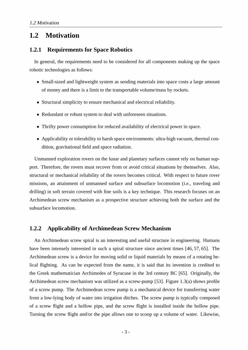
the Greek mathematician Archimedes of Syracuse in the 3rd century BC [65]. Originally, the
Archimedean screw mechanism was utilized as a screw-pump [53]. Figure 1.3(a) shows profile
of a screw pump. The Archimedean screw pump is a mechanical device for transferring water
from a low-lying body of water into irrigation ditches. The screw pump is typically composed
of a screw flight and a hollow pipe, and the screw flight is installed inside the hollow pipe.
Turning the screw flight and/or the pipe allows one to scoop up a volume of water. Likewise,
- 3 -
1.3 Purpose and Approach
the Archimedean screw mechanism has been used for conveying not only liquid but granular
materials [49, 56, 58]. As for the screw conveyors, some has studied their theoretical analysis
such as a transportation efficiency. However, the screw is fixed and just motions of transported
materials is considered.
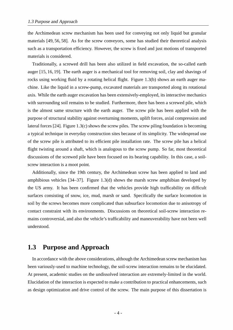
Traditionally, a screwed drill has been also utilized in field excavation, the so-called earth
auger [15, 16, 19]. The earth auger is a mechanical tool for removing soil, clay and shavings of
rocks using working fluid by a rotating helical flight. Figure 1.3(b) shows an earth auger ma-
chine. Like the liquid in a screw-pump, excavated materials are transported along its rotational
axis. While the earth auger excavation has been extensively-employed, its interactive mechanics
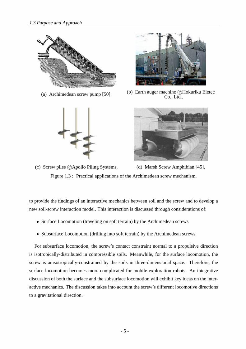
with surrounding soil remains to be studied. Furthermore, there has been a screwed pile, which
is the almost same structure with the earth auger. The screw pile has been applied with the
purpose of structural stability against overturning moments, uplift forces, axial compression and
lateral forces [24]. Figure 1.3(c) shows the screw piles. The screw piling foundation is becoming
a typical technique in everyday construction sites because of its simplicity. The widespread use
of the screw pile is attributed to its efficient pile installation rate. The screw pile has a helical
flight twisting around a shaft, which is analogous to the screw pump. So far, most theoretical
discussions of the screwed pile have been focused on its bearing capability. In this case, a soil-
screw interaction is a moot point.
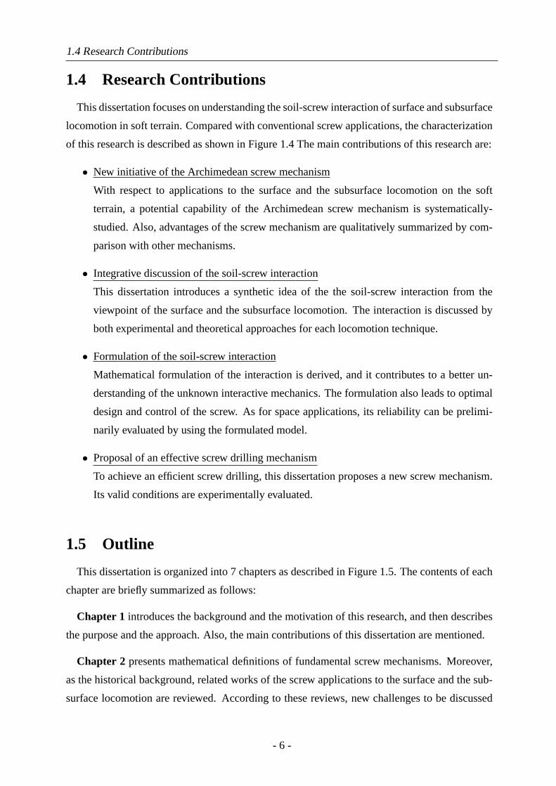
Additionally, since the 19th century, the Archimedean screw has been applied to land and
amphibious vehicles [34–37]. Figure 1.3(d) shows the marsh screw amphibian developed by
the US army. It has been confirmed that the vehicles provide high trafficability on difficult
surfaces consisting of snow, ice, mud, marsh or sand. Specifically the surface locomotion in
soil by the screws becomes more complicated than subsurface locomotion due to anisotropy of
contact constraint with its environments. Discussions on theoretical soil-screw interaction re-
mains controversial, and also the vehicle’s trafficability and maneuverability have not been well
understood.
1.3 Purpose and Approach
In accordance with the above considerations, although the Archimedean screw mechanism has
been variously-used to machine technology, the soil-screw interaction remains to be elucidated.
At present, academic studies on the undissolved interaction are extremely-limited in the world.
Elucidation of the interaction is expected to make a contribution to practical enhancements, such
as design optimization and drive control of the screw. The main purpose of this dissertation is
- 4 -
1.3 Purpose and Approach
(a) Archimedean screw pump [50]. (b) Earth auger machinec©Hokuriku EletecCo., Ltd..
(c) Screw pilesc©Apollo Piling Systems. (d) Marsh Screw Amphibian [45].
Figure 1.3 : Practical applications of the Archimedean screw mechanism.
to provide the findings of an interactive mechanics between soil and the screw and to develop a
new soil-screw interaction model. This interaction is discussed through considerations of:
• Surface Locomotion (traveling on soft terrain) by the Archimedean screws
• Subsurface Locomotion (drilling into soft terrain) by the Archimedean screws
For subsurface locomotion, the screw’s contact constraint normal to a propulsive direction
is isotropically-distributed in compressible soils. Meanwhile, for the surface locomotion, the
screw is anisotropically-constrained by the soils in three-dimensional space. Therefore, the
surface locomotion becomes more complicated for mobile exploration robots. An integrative
discussion of both the surface and the subsurface locomotion will exhibit key ideas on the inter-
active mechanics. The discussion takes into account the screw’s different locomotive directions
to a gravitational direction.
- 5 -
1.4 Research Contributions
1.4 Research Contributions
This dissertation focuses on understanding the soil-screw interaction of surface and subsurface
locomotion in soft terrain. Compared with conventional screw applications, the characterization
of this research is described as shown in Figure 1.4 The main contributions of this research are:
• New initiative of the Archimedean screw mechanism
With respect to applications to the surface and the subsurface locomotion on the soft
terrain, a potential capability of the Archimedean screw mechanism is systematically-
studied. Also, advantages of the screw mechanism are qualitatively summarized by com-
parison with other mechanisms.
• Integrative discussion of the soil-screw interaction
This dissertation introduces a synthetic idea of the the soil-screw interaction from the
viewpoint of the surface and the subsurface locomotion. The interaction is discussed by
both experimental and theoretical approaches for each locomotion technique.
• Formulation of the soil-screw interaction
Mathematical formulation of the interaction is derived, and it contributes to a better un-
derstanding of the unknown interactive mechanics. The formulation also leads to optimal
design and control of the screw. As for space applications, its reliability can be prelimi-
narily evaluated by using the formulated model.
• Proposal of an effective screw drilling mechanism
To achieve an efficient screw drilling, this dissertation proposes a new screw mechanism.
Its valid conditions are experimentally evaluated.
1.5 Outline
This dissertation is organized into 7 chapters as described in Figure 1.5. The contents of each
chapter are briefly summarized as follows:
Chapter 1 introduces the background and the motivation of this research, and then describes
the purpose and the approach. Also, the main contributions of this dissertation are mentioned.
Chapter 2 presents mathematical definitions of fundamental screw mechanisms. Moreover,
as the historical background, related works of the screw applications to the surface and the sub-
surface locomotion are reviewed. According to these reviews, new challenges to be discussed
- 6 -
1.5 Outline
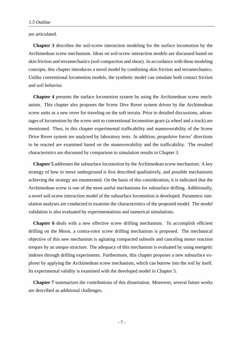
are articulated.
Chapter 3 describes the soil-screw interaction modeling for the surface locomotion by the
Archimedean screw mechanism. Ideas on soil-screw interaction models are discussed based on
skin friction and terramechanics (soil compaction and shear). In accordance with these modeling
concepts, this chapter introduces a novel model by combining skin friction and terramechanics.
Unlike conventional locomotion models, the synthetic model can simulate both contact friction
and soil behavior.
Chapter 4 presents the surface locomotion system by using the Archimedean screw mech-
anism. This chapter also proposes the Screw Dive Rover system driven by the Archimedean
screw units as a new rover for traveling on the soft terrain. Prior to detailed discussions, advan-
tages of locomotion by the screw unit to conventional locomotion gears (a wheel and a track) are
mentioned. Then, in this chapter experimental trafficability and maneuverability of the Screw
Drive Rover system are analyzed by laboratory tests. In addition, propulsive forces’ directions
to be reacted are examined based on the maneuverability and the trafficability. The resulted
characteristics are discussed by comparison to simulation results in Chapter 3.
Chapter 5addresses the subsurface locomotion by the Archimedean screw mechanism. A key
strategy of how to move underground is first described qualitatively, and possible mechanisms
achieving the strategy are enumerated. On the basis of this consideration, it is indicated that the
Archimedean screw is one of the most useful mechanisms for subsurface drilling. Additionally,
a novel soil-screw interaction model of the subsurface locomotion is developed. Parametric sim-
ulation analyses are conducted to examine the characteristics of the proposed model. The model
validation is also evaluated by experimentations and numerical simulations.
Chapter 6 deals with a new effective screw drilling mechanism. To accomplish efficient
drilling on the Moon, a contra-rotor screw drilling mechanism is proposed. The mechanical
objective of this new mechanism is agitating compacted subsoils and canceling motor reaction
torques by an unique structure. The adequacy of this mechanism is evaluated by using energetic
indexes through drilling experiments. Furthermore, this chapter proposes a new subsurface ex-
plorer by applying the Archimedean screw mechanism, which can burrow into the soil by itself.
Its experimental validity is examined with the developed model in Chapter 5.
Chapter 7 summarizes the contributions of this dissertation. Moreover, several future works
are described as additional challenges.
- 7 -
1.5 Outline
Arc
him
ed
ean
Scre
w M
ech
an
ism
Su
bsu
race L
oco
mo
tio
n (
Dri
llin
g)
Su
race L
oco
mo
tio
n (
Tra
velin
g)
Co
nta
ct
Co
nstr
ain
t:
iso
tro
pic
ally
-go
ve
rne
d b
y c
om
pre
ssib
le s
oil
Co
nta
ct
Co
nstr
ain
t:
an
iso
tro
pic
ally
-go
ve
rne
d b
y c
om
pre
ssib
le s
oil
Co
nve
ntio
na
l R
ese
arc
h
Ea
rth
Au
ge
r
-
wid
esp
rea
d u
se
in
co
nstr
uctio
n
-
inve
stig
atio
n o
f g
eo
me
tic e
ffe
cts
Scre
we
d P
ile
-
dis
cu
ssio
n o
f b
ea
rin
g c
ap
ab
ility
-
inve
stig
atio
n o
f g
eo
me
tic e
ffe
cts
-
limite
d m
ath
em
atica
l m
od
elin
g
Co
nve
ntio
na
l R
ese
arc
h
Ch
alle
ng
es
- u
nd
ers
tan
din
g o
f so
il-scre
w
in
tera
ctio
n m
ech
an
sim
- m
ath
em
atica
l m
od
elin
g o
f
s
oil-
scre
w in
tera
ctio
n
- m
ech
an
ica
l im
pro
ve
me
nt
for
eff
ective
scre
w m
ech
an
ism
Ch
alle
ng
es
- u
nd
ers
tan
din
g o
f so
il-scre
w
in
tera
ctio
n m
ech
an
sim
- m
ath
em
atica
l m
od
elin
g o
f
so
il-scre
w in
tera
ctio
n
- syste
ma
tic in
ve
stig
atio
ns o
f
mo
bilt
y p
erf
orm
an
ce
Co
nveyo
r
- w
ate
r
- g
ranula
r
m
ate
rials
Pro
peller
- v
essel
- u
nderw
ate
r
ro
bot
Oth
er
Ap
plicati
on
s
- .........
- .........
- .........
- .........
- .........
- .........
- .........
- .........
- .........
Po
ten
tial
Ap
plicati
on
Th
is D
issert
ati
on
Co
ntr
ibu
tio
n
Ma
rsh
Scre
w A
mp
hib
ian
-
limite
d e
mp
iric
al e
lab
ora
tio
ns
-
inve
stig
atio
n o
f a
fe
w s
cre
w
ge
om
etr
ic e
ffe
cts
-
ma
ny p
ate
nts
(e
.g.
ve
hic
le,
ho
bb
y)
-
limite
d m
ath
em
atica
l m
od
elin
g
Fig
ure
1.4
:C
hara
cter
izat
ion
ofth
isdi
sser
tatio
n.
- 8 -
1.5 Outline
Chapter 1 Introduction
1. Background
2. Motivation and Challenge
3. Objective
4. Contributions
Chapter 5 Modeling and Analysis
1. [Statement] Technological background
2. [Proposal] Locomotion strategy
3. [Proposal] Soil-screw interaction model
4. [Validation] Experiments and simulations
Subsurface LocomotionSurface Locomotion
Chapter 6 Proposal of Effective
Screw Drilling and Total Systemg
1. [Propose] Contra-rotor screw drill
2. [Validation] Experimenatal analyses
3. [Proposal] Subsurface screw explorer
4. [Validation] Experimens and simulations
Outline of Thesis
Theme: Understanding of Soil-Screw Interaction
Traveling on Soft Terrain Driling into Soft Terrain
Chapter 4 Experimental Analyses
1. [Statement] Technological background
2. [Proposal] Screw Drive Rover system
3. [Analysis] Empirical maneuverability
4. [Analysis] Empirical trafficabiliy
5. [Discussion] Compatible force model
Chapter 3 Modeling and Analysis
1. [Proposal] Soil-screw interaction model
- modeling based on skin friction
- modeling based on terramechanics
2. [Validation] Simulation analyses
Chapter 7 Conclusions
1. Summarizing remarks
2. Future works
Chapter 2 Archimedean Screw
1. Overview Archimedean Screw
2. Related Works
3. Mathematical Definitions of
Fundamental Screw Geometry
Figure 1.5 : Configured outline of this dissertation.
- 9 -

1.5 Outline
- 10 -
Chapter 2. Archimedean Screw
Mechanism
An Archimedean screw mechanism is an attractive structure and has been used in various
applications as described in Chapter 1. This dissertation especially focuses on its application
to surface and subsurface locomotion in soft terrain (i.e., traveling on surface and drilling into
subsurface). In the meantime, studies on the screw has been quite limited and it includes a lot
of missing parts academically. To apply it to deformable terrain such as soil, theoretical and
systematic discussions are required. First of all, this chapter derives mathematical definitions of
fundamental screw mechanisms as preliminary matters for the subsequent chapters.
2.1 Geometric Modeling of Screw Mechanism
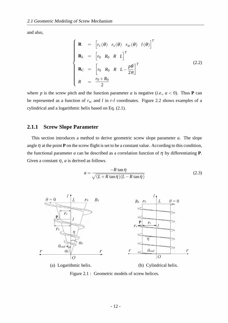
In this dissertation, two types of the Archimedean screw mechanisms are considered: a loga-
rithmic and a cylindrical helix. Hereη denotes the constant inclination angle of screw flight at
the center positionP on the screw flights. As common terms, the screw length isL, the maximum
inner radius of the screws isr0 and the maximum screw radius isR0. In addition, logarithmic and
cylindrical screw models can be mathematically expressed as a function of the winding screw
angleθ against a cone and a cylinder in Figure 2.1. Also, the screw thickness is neglected. As
coordinates,l axis is set to be the central axis of the explorer, andr is defined as the distance
from l axis as shown in Figure 2.1, respectively. Furthermore,l denotes the height from the apex
of the screw andθ is set to be zero at the highest position of the screws. At a winding angleθ ,
rc, rs, andrsc are defined as the inner screw radius, the outer screw radius, and the distance from
l axis toP, respectively. The mathematic models of the helices can be defined as follows.
R =
RL exp(aθ) : Logarithmic Helix
RC : Cylindrical Helix(2.1)
- 11 -
2.1 Geometric Modeling of Screw Mechanism
and also,
R =[rc(θ) rs(θ) rsc(θ) l (θ)
]T
RL =[r0 R0 R L
]T
RC =[r0 R0 R L− pθ
2π
]T
R =r0 +R0
2
(2.2)
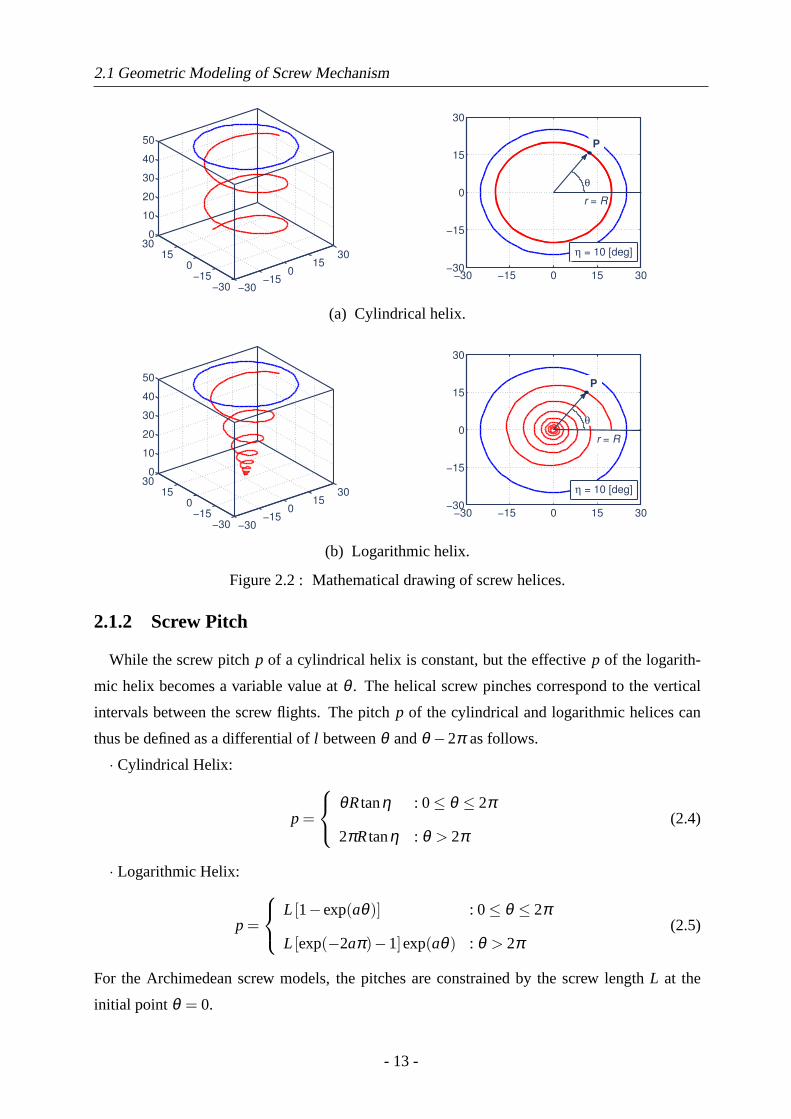
wherep is the screw pitch and the function parametera is negative (i.e., a < 0). ThusP can
be represented as a function ofrsc and l in r-l coordinates. Figure 2.2 shows examples of a
cylindrical and a logarithmic helix based on Eq. (2.1).
2.1.1 Screw Slope Parameter
This section introduces a method to derive geometric screw slope parametera. The slope
angleη at the pointPon the screw flight is set to be a constant value. According to this condition,
the functional parametera can be described as a correlation function ofη by differentiatingP.
Given a constantη , a is derived as follows.
a =−R tanη√
(L+R tanη)(L−R tanη)(2.3)
(a) Logarithmic helix. (b) Cylindrical helix.
Figure 2.1 : Geometric models of screw helices.
- 12 -
2.1 Geometric Modeling of Screw Mechanism
−30−15
015
30
−30
−15
0
15
300
10
20
30
40
50
−30 −15 0 15 30−30
−15
0
15
30
θ
r = R
P
η = 10 [deg]
(a) Cylindrical helix.
−30−15
015
30
−30
−15
0
15
300
10
20
30
40
50
−30 −15 0 15 30−30
−15
0
15
30
θ
η = 10 [deg]
P
r = R
(b) Logarithmic helix.
Figure 2.2 : Mathematical drawing of screw helices.
2.1.2 Screw Pitch
While the screw pitchp of a cylindrical helix is constant, but the effectivep of the logarith-
mic helix becomes a variable value atθ . The helical screw pinches correspond to the vertical
intervals between the screw flights. The pitchp of the cylindrical and logarithmic helices can
thus be defined as a differential ofl betweenθ andθ −2π as follows.
· Cylindrical Helix:
p =
θRtanη : 0≤ θ ≤ 2π
2πRtanη : θ > 2π(2.4)
· Logarithmic Helix:
p =
L [1−exp(aθ)] : 0≤ θ ≤ 2π
L [exp(−2aπ)−1]exp(aθ) : θ > 2π(2.5)
For the Archimedean screw models, the pitches are constrained by the screw lengthL at the
initial point θ = 0.
- 13 -
2.2 Related Works
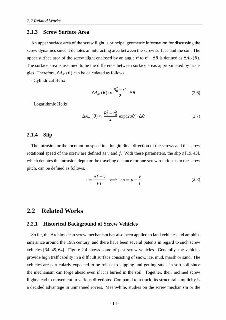
2.1.3 Screw Surface Area
An upper surface area of the screw flight is principal geometric information for discussing the
screw dynamics since it denotes an interacting area between the screw surface and the soil. The
upper surface area of the screw flight enclosed by an angleθ to θ + ∆θ is defined as∆Asc(θ).
The surface area is assumed to be the difference between surface areas approximated by trian-
gles. Therefore,∆Asc(θ) can be calculated as follows.
· Cylindrical Helix:
∆Asc(θ)≈ R20− r2
0
2·∆θ (2.6)
· Logarithmic Helix:
∆Asc(θ)≈ R20− r2
0
2exp(2aθ) ·∆θ (2.7)
2.1.4 Slip
The intrusion or the locomotion speed in a longitudinal direction of the screws and the screw
rotational speed of the screw are defined asv and f . With these parameters, the slips [19, 43],
which denotes the intrusion depth or the traveling distance for one screw rotation as to the screw
pitch, can be defined as follows.
s=p f−v
p f⇐⇒ sp= p− v
f(2.8)
2.2 Related Works
2.2.1 Historical Background of Screw Vehicles
So far, the Archimedean screw mechanism has also been applied to land vehicles and amphib-
ians since around the 19th century, and there have been several patents in regard to such screw
vehicles [34–45, 64]. Figure 2.4 shows some of past screw vehicles. Generally, the vehicles
provide high trafficability in a difficult surface consisting of snow, ice, mud, marsh or sand. The
vehicles are particularly expected to be robust to slipping and getting stuck in soft soil since
the mechanism can forge ahead even if it is buried in the soil. Together, their inclined screw
flights lead to movement in various directions. Compared to a track, its structural simplicity is
a decided advantage in unmanned rovers. Meanwhile, studies on the screw mechanism or the
- 14 -
2.2 Related Works
0 10 20 30 40 50 60−1
−0.5
0
−0.25
−0.75
Screw Slope Angle, η [deg]
Helical P
ara
mete
r, a
R = 0.02 [m]
L = 0.05 [m]
(a) Relationship betweena andη .
0 20 40 600
1
2
3
4
5x 10
−4
Screw Angle, θ [rad]
∆A
sc/∆
θ [m
2/r
ad]
R0 = 0.025 [m]
r0 = 0.015 [m]
a = −0.070707
(b) Relationship between∆Asc/∆θ andη .
0 20 40 600
0.005
0.01
0.015
0.02
Screw Angle, θ [rad]
Scre
w P
itch, p [m
]
2π
L = 0.05 [m]
a = −0.070707
(c) Relationship betweenp andθ .
Figure 2.3 : Functional behaviors of logarithmic screw geometry.
vehicle have been extremely limited [38, 41, 43, 64]. Consequently, an actual soil-screw inter-
action remains to be elucidated from academic viewpoint. In such background of the vehicles,
theoretical discussions of the screw vehicle have been conducted by Cole [38]. This work has
attempted to analytically model and evaluate the vehicle’s traction performance on sand, but its
model was developed based on just skin friction and ignored both slippage and soil shear phe-
nomena. Therefore, the model is inadequate to be applied. On the other hand, Dugoffet al. [43]
especially examined the characteristics between translatory traction and a slip of a single screw
- 15 -
2.2 Related Works
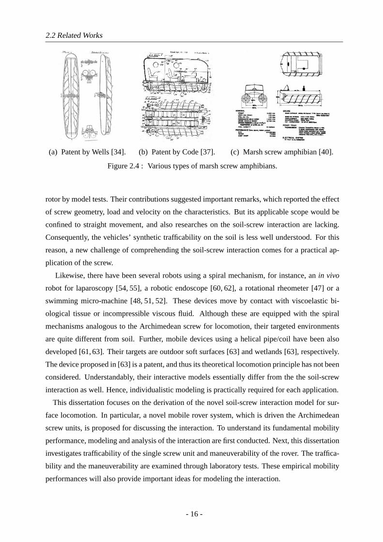
(a) Patent by Wells [34]. (b) Patent by Code [37]. (c) Marsh screw amphibian [40].
Figure 2.4 : Various types of marsh screw amphibians.
rotor by model tests. Their contributions suggested important remarks, which reported the effect
of screw geometry, load and velocity on the characteristics. But its applicable scope would be
confined to straight movement, and also researches on the soil-screw interaction are lacking.
Consequently, the vehicles’ synthetic trafficability on the soil is less well understood. For this
reason, a new challenge of comprehending the soil-screw interaction comes for a practical ap-
plication of the screw.
Likewise, there have been several robots using a spiral mechanism, for instance, anin vivo
robot for laparoscopy [54, 55], a robotic endoscope [60, 62], a rotational rheometer [47] or a
swimming micro-machine [48, 51, 52]. These devices move by contact with viscoelastic bi-
ological tissue or incompressible viscous fluid. Although these are equipped with the spiral
mechanisms analogous to the Archimedean screw for locomotion, their targeted environments
are quite different from soil. Further, mobile devices using a helical pipe/coil have been also
developed [61, 63]. Their targets are outdoor soft surfaces [63] and wetlands [63], respectively.
The device proposed in [63] is a patent, and thus its theoretical locomotion principle has not been
considered. Understandably, their interactive models essentially differ from the the soil-screw
interaction as well. Hence, individualistic modeling is practically required for each application.
This dissertation focuses on the derivation of the novel soil-screw interaction model for sur-
face locomotion. In particular, a novel mobile rover system, which is driven the Archimedean
screw units, is proposed for discussing the interaction. To understand its fundamental mobility
performance, modeling and analysis of the interaction are first conducted. Next, this dissertation
investigates trafficability of the single screw unit and maneuverability of the rover. The traffica-
bility and the maneuverability are examined through laboratory tests. These empirical mobility
performances will also provide important ideas for modeling the interaction.
- 16 -
2.2 Related Works
2.2.2 Historical Background of Screw Drilling
The screw drilling devices basically consist of a single unit with a cylinder/cone and a continu-
ous helical screw flighting. Until now, they has been used as ground applications to construction
field such as an earth-auger (e.g.[15,16,19]) and a screw pile (e.g.[24]) as described in Chapter
1. Initially, a auger drilling tool was used as a grain auger agriculture to move grain from trucks
and grain carts into grain storage bins. It is said the modern grain auger was first prototyped by
Peter Pakosh in 1945. On the other hand, the original screw pile was invented by Irish engineer
Alexander Mitchell in 1833 [24]. Although its structural design was simple, the screw pile was
utilized as effective means of construction for lighthouses, beacons, moorings and other struc-
tures on muddy banks or shifting sands.
In general, these screw devices have the following important capabilities for a subsurface
drilling technique:
• Backward fore-soil removal and transportation (achievement of making a space)
• Genesis of assisting force for intrusion by transporting fore-soil
• Dust prevention mechanism
The Archimedean screw mechanism is one of the most prospective drilling tools. Basically, a
machined thread is superior in terms of intrusion with cutting materials. However it is not great
at generating propulsive force by screw rotations because of the thread profile. Therefore, screw
flights composed of flat and helical blades have been adopted as described in the subsequent
subsections. Such screw mechanism is particularly expected to be suitable for drilling into com-
pacted soil layer.
Meanwhile, many theoretical parts of the screw drilling remain to be elaborated. So far, there
have some theoretical approaches [18, 19, 23, 30]. Hataet al. [18, 19] and Slatteret al. [23]
have discussed the soil-screw interaction of the screw drilling. However, their models involve
many theoretical insufficiencies as to definitions of forces, and the practical applicability of
the models are not clear. Additionally, Fukadaet al. [30] have studied the soil discharging
model. In the modeling process, the soil-screw interaction has been also represented as prelim-
inary definitions. But the model also includes lacking parts of acting forces and an unknown
force remains to be defined. As for the screw piles, some have also addressed theoretical dis-
cussions [21, 22, 28, 29, 31, 32]. The theoretical analyses on the screw piles have particularly
focused on an evaluation of their bearing capability. Accordingly, most of them have not mod-
eled the soil-screw interaction. For realizing an effective and autonomous screw mechanism, its
- 17 -
2.3 Summary
modeling is a new challenge. Unlike most ground applications, unmanned exploration robots do
not allow for human intervention. Therefore, mechanical reliability and high efficiency based
on theoretical analyses should be proved for practical applications of the screw.
This dissertation aims at the derivation of the novel soil-screw interaction model for subsur-
face drilling. The model is introduced based on soil mechanics with screw behavior. Unlike
the surface locomotion model, influences in a direction of gravitational force are particularly
involved. Of particular note is that the fundamentals of the model is analogous to the model for
surface locomotion.
2.3 Summary
Understanding an interactive mechanics between a mechanical tool and environment is quite
important for unmanned robotic explorations. Not only the screw mechanisms, but all the tools
in the soft terrain need mathematical modeling in order to efficiently use them. In this chap-
ter, prior to detailed discussions of the soil-screw interaction, some of geometric and kinematic
definitions of the helical screws were introduced. By considering them, the interaction models
will be provided as functions of the screw geometry. Furthermore, the historical backgrounds
with respect to screw drilling and screw vehicles were introduced from the viewpoint of their
theoretical frameworks. According to these remarks, the necessity for developing a new interac-
tion modeling was pointed out. This chapter reaffirmed that the development of the soil-screw
interaction model is the key challenge to be addressed.
- 18 -
Chapter 3. Modeling of Screw Surface
Locomotion
3.1 Challenge Statement for Robotic Surface Locomotion
Robotic exploration by mobile rovers has received attention worldwide for the achievement
of progressive space missions. In the history of space exploration, Lunokhod 1 and 2 built by
the Soviet Union were the first unmanned rovers [113, 115, 116]. These huge rovers moved
onto the lunar surface in 1970 and 1973, and were teleoperated from Earth. Recently, the So-
journer rover [117] and the Mars Exploration Rovers (MERs) [123] operated by NASA have
performed impressive exploration activities on Mars. They employ six wheels for traveling over
the Martian surface, and the MERs have especially acquired scientific findings for more than 6
years [124, 126, 138]. In their locomotion mechanism, these three rovers have the rocker-bogie
suspension mechanism to traverse rocky terrains [125]. Until now, there have been some lunar
and planetary rovers adopted in actual missions as shown in Table 3.1 and Figure 3.1. Most of
them employ wheels as their locomotion system because of reliability, simplicity and efficiency.
Although the wheels were not selected to especially move on an asteroid’s surface under micro-
gravity (e.g., PROP-F [116, 118] or MINERVA [121]), the wheels have contributed most to the
exploration rovers (see Table 3.1). Meanwhile, the MER Spirit rover, one of the two MERs, has
been mired in a Martian version of quicksand since May 2009 [13,137]. Mission engineers have
investigated how the rover might extricate itself from the sand trap by indoor experimentation
and computer simulation as shown in Figure 3.2. However, on January 2010, it was announced
NASA ended its removal attempts [14]. This result dramatically indicates limitations of wheeled
locomotion on soft soil such as lunar and Martian regolith. Therefore, advanced gears or im-
proved wheels must be newly developed to cope with such a difficult terrain due to the tractive
limitations of the wheel discussed in Appendix B.
Generally, typical locomotion gears are classified into wheeled, tracked and legged locomo-
tion. There have been some proposals of tracked rovers [74, 135, 136] and legged rovers [122].
In addition to these typical ones, hybrid-typed locomotion gears have also been considered, such
as a leg-wheel [129, 131] or a leg-track [139]. For now, the hybrid-typed gears would have just
- 19 -
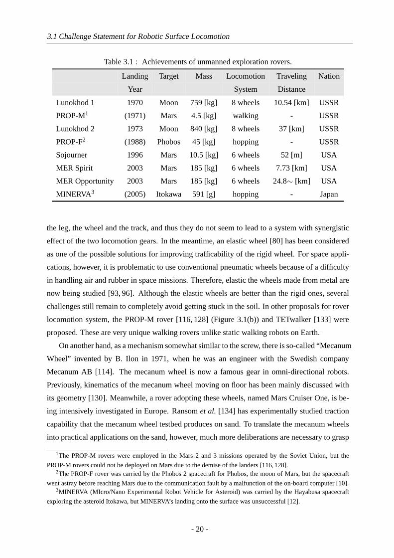
3.1 Challenge Statement for Robotic Surface Locomotion
Table 3.1 : Achievements of unmanned exploration rovers.
Landing Target Mass Locomotion Traveling Nation
Year System Distance
Lunokhod 1 1970 Moon 759 [kg] 8 wheels 10.54 [km] USSR
PROP-M1 (1971) Mars 4.5 [kg] walking - USSR
Lunokhod 2 1973 Moon 840 [kg] 8 wheels 37 [km] USSR
PROP-F2 (1988) Phobos 45 [kg] hopping - USSR
Sojourner 1996 Mars 10.5 [kg] 6 wheels 52 [m] USA
MER Spirit 2003 Mars 185 [kg] 6 wheels 7.73 [km] USA
MER Opportunity 2003 Mars 185 [kg] 6 wheels 24.8∼ [km] USA
MINERVA3 (2005) Itokawa 591 [g] hopping - Japan
the leg, the wheel and the track, and thus they do not seem to lead to a system with synergistic
effect of the two locomotion gears. In the meantime, an elastic wheel [80] has been considered
as one of the possible solutions for improving trafficability of the rigid wheel. For space appli-
cations, however, it is problematic to use conventional pneumatic wheels because of a difficulty
in handling air and rubber in space missions. Therefore, elastic the wheels made from metal are
now being studied [93, 96]. Although the elastic wheels are better than the rigid ones, several
challenges still remain to completely avoid getting stuck in the soil. In other proposals for rover
locomotion system, the PROP-M rover [116, 128] (Figure 3.1(b)) and TETwalker [133] were
proposed. These are very unique walking rovers unlike static walking robots on Earth.
On another hand, as a mechanism somewhat similar to the screw, there is so-called “Mecanum
Wheel” invented by B. Ilon in 1971, when he was an engineer with the Swedish company
Mecanum AB [114]. The mecanum wheel is now a famous gear in omni-directional robots.
Previously, kinematics of the mecanum wheel moving on floor has been mainly discussed with
its geometry [130]. Meanwhile, a rover adopting these wheels, named Mars Cruiser One, is be-
ing intensively investigated in Europe. Ransomet al. [134] has experimentally studied traction
capability that the mecanum wheel testbed produces on sand. To translate the mecanum wheels
into practical applications on the sand, however, much more deliberations are necessary to grasp
1The PROP-M rovers were employed in the Mars 2 and 3 missions operated by the Soviet Union, but the
PROP-M rovers could not be deployed on Mars due to the demise of the landers [116,128].2The PROP-F rover was carried by the Phobos 2 spacecraft for Phobos, the moon of Mars, but the spacecraft
went astray before reaching Mars due to the communication fault by a malfunction of the on-board computer [10].3MINERVA (MIcro/Nano Experimental Robot Vehicle for Asteroid) was carried by the Hayabusa spacecraft
exploring the asteroid Itokawa, but MINERVA’s landing onto the surface was unsuccessful [12].
- 20 -
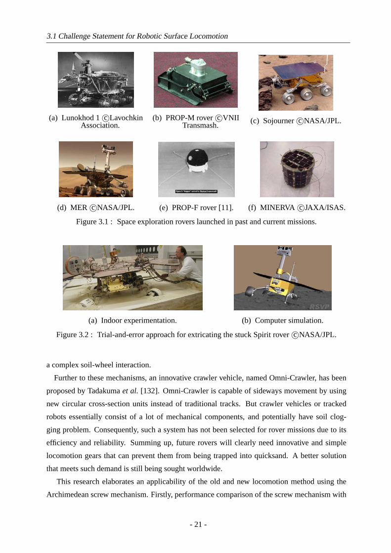
3.1 Challenge Statement for Robotic Surface Locomotion
(a) Lunokhod 1c©LavochkinAssociation.
(b) PROP-M roverc©VNIITransmash.
(c) Sojournerc©NASA/JPL.
(d) MER c©NASA/JPL. (e) PROP-F rover [11]. (f) MINERVA c©JAXA/ISAS.
Figure 3.1 : Space exploration rovers launched in past and current missions.
(a) Indoor experimentation. (b) Computer simulation.
Figure 3.2 : Trial-and-error approach for extricating the stuck Spirit roverc©NASA/JPL.
a complex soil-wheel interaction.
Further to these mechanisms, an innovative crawler vehicle, named Omni-Crawler, has been
proposed by Tadakumaet al. [132]. Omni-Crawler is capable of sideways movement by using
new circular cross-section units instead of traditional tracks. But crawler vehicles or tracked
robots essentially consist of a lot of mechanical components, and potentially have soil clog-
ging problem. Consequently, such a system has not been selected for rover missions due to its
efficiency and reliability. Summing up, future rovers will clearly need innovative and simple
locomotion gears that can prevent them from being trapped into quicksand. A better solution
that meets such demand is still being sought worldwide.
This research elaborates an applicability of the old and new locomotion method using the
Archimedean screw mechanism. Firstly, performance comparison of the screw mechanism with
- 21 -
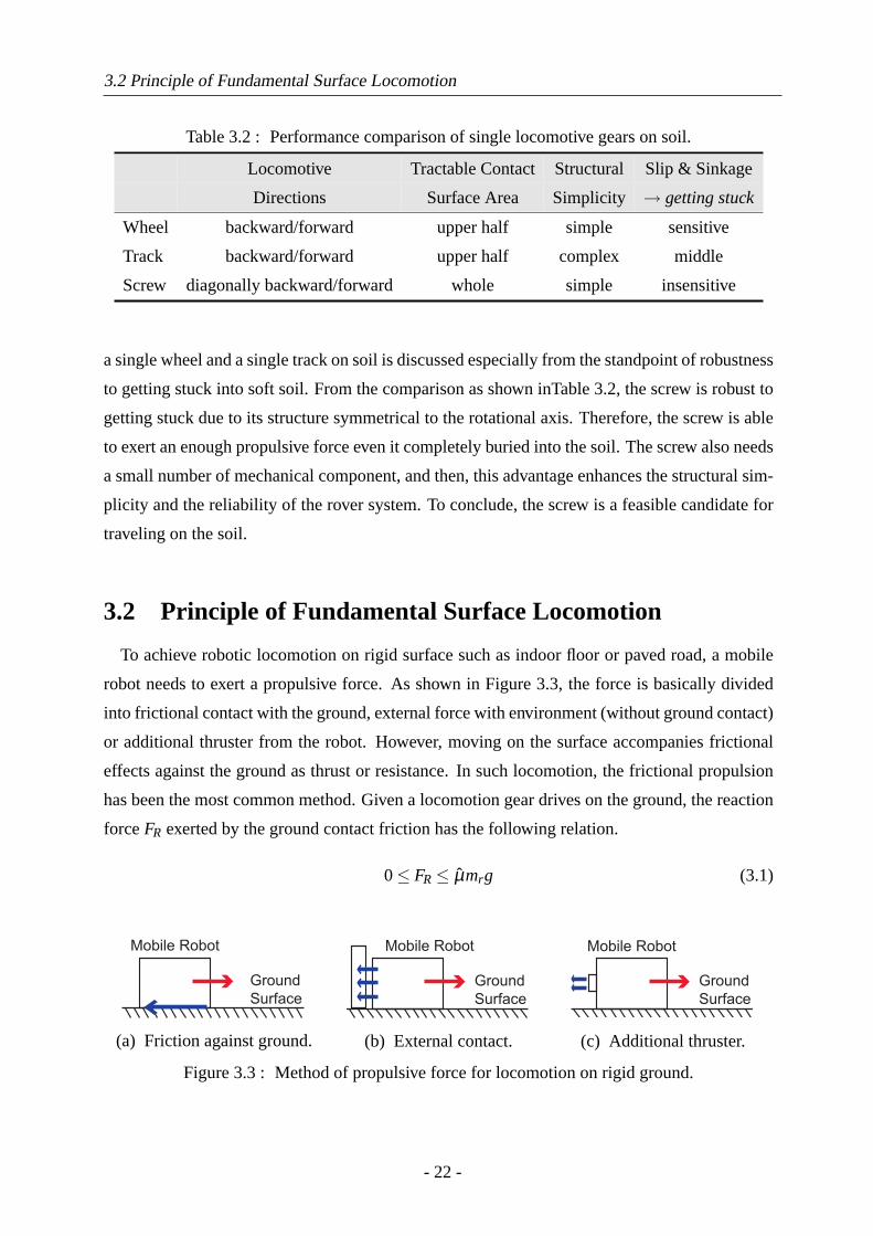
3.2 Principle of Fundamental Surface Locomotion
Table 3.2 : Performance comparison of single locomotive gears on soil.
Locomotive Tractable Contact Structural Slip & Sinkage
Directions Surface Area Simplicity → getting stuck
Wheel backward/forward upper half simple sensitive
Track backward/forward upper half complex middle
Screw diagonally backward/forward whole simple insensitive
a single wheel and a single track on soil is discussed especially from the standpoint of robustness
to getting stuck into soft soil. From the comparison as shown inTable 3.2, the screw is robust to
getting stuck due to its structure symmetrical to the rotational axis. Therefore, the screw is able
to exert an enough propulsive force even it completely buried into the soil. The screw also needs
a small number of mechanical component, and then, this advantage enhances the structural sim-
plicity and the reliability of the rover system. To conclude, the screw is a feasible candidate for
traveling on the soil.
3.2 Principle of Fundamental Surface Locomotion
To achieve robotic locomotion on rigid surface such as indoor floor or paved road, a mobile
robot needs to exert a propulsive force. As shown in Figure 3.3, the force is basically divided
into frictional contact with the ground, external force with environment (without ground contact)
or additional thruster from the robot. However, moving on the surface accompanies frictional
effects against the ground as thrust or resistance. In such locomotion, the frictional propulsion
has been the most common method. Given a locomotion gear drives on the ground, the reaction
forceFR exerted by the ground contact friction has the following relation.
0≤ FR≤ µmrg (3.1)
Mobile Robot
Ground
Surface
(a) Friction against ground.
Mobile Robot
Ground
Surface
(b) External contact.
Mobile Robot
Ground
Surface
(c) Additional thruster.
Figure 3.3 : Method of propulsive force for locomotion on rigid ground.
- 22 -
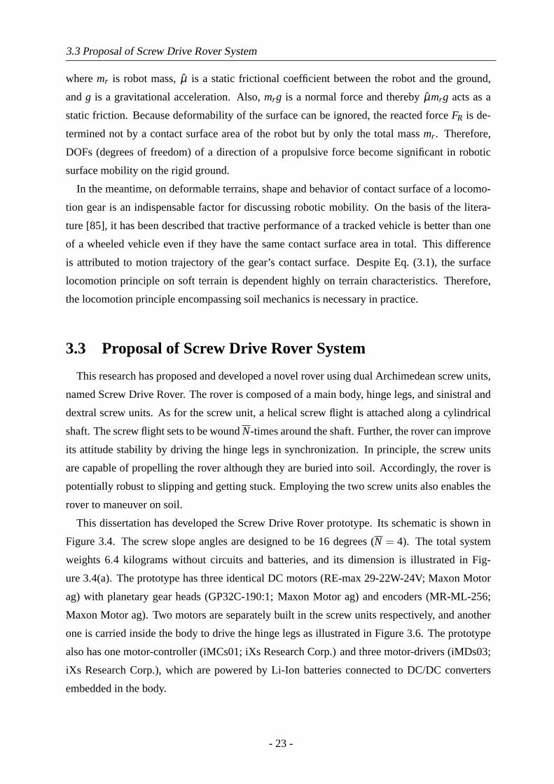
3.3 Proposal of Screw Drive Rover System
wheremr is robot mass,µ is a static frictional coefficient between the robot and the ground,
andg is a gravitational acceleration. Also,mrg is a normal force and therebyµmrg acts as a
static friction. Because deformability of the surface can be ignored, the reacted forceFR is de-
termined not by a contact surface area of the robot but by only the total massmr . Therefore,
DOFs (degrees of freedom) of a direction of a propulsive force become significant in robotic
surface mobility on the rigid ground.
In the meantime, on deformable terrains, shape and behavior of contact surface of a locomo-
tion gear is an indispensable factor for discussing robotic mobility. On the basis of the litera-
ture [85], it has been described that tractive performance of a tracked vehicle is better than one
of a wheeled vehicle even if they have the same contact surface area in total. This difference
is attributed to motion trajectory of the gear’s contact surface. Despite Eq. (3.1), the surface
locomotion principle on soft terrain is dependent highly on terrain characteristics. Therefore,
the locomotion principle encompassing soil mechanics is necessary in practice.
3.3 Proposal of Screw Drive Rover System
This research has proposed and developed a novel rover using dual Archimedean screw units,
named Screw Drive Rover. The rover is composed of a main body, hinge legs, and sinistral and
dextral screw units. As for the screw unit, a helical screw flight is attached along a cylindrical
shaft. The screw flight sets to be woundN-times around the shaft. Further, the rover can improve
its attitude stability by driving the hinge legs in synchronization. In principle, the screw units
are capable of propelling the rover although they are buried into soil. Accordingly, the rover is
potentially robust to slipping and getting stuck. Employing the two screw units also enables the
rover to maneuver on soil.
This dissertation has developed the Screw Drive Rover prototype. Its schematic is shown in
Figure 3.4. The screw slope angles are designed to be16 degrees (N = 4). The total system
weights6.4 kilograms without circuits and batteries, and its dimension is illustrated in Fig-
ure 3.4(a). The prototype has three identical DC motors (RE-max 29-22W-24V; Maxon Motor
ag) with planetary gear heads (GP32C-190:1; Maxon Motor ag) and encoders (MR-ML-256;
Maxon Motor ag). Two motors are separately built in the screw units respectively, and another
one is carried inside the body to drive the hinge legs as illustrated in Figure 3.6. The prototype
also has one motor-controller (iMCs01; iXs Research Corp.) and three motor-drivers (iMDs03;
iXs Research Corp.), which are powered by Li-Ion batteries connected to DC/DC converters
embedded in the body.
- 23 -
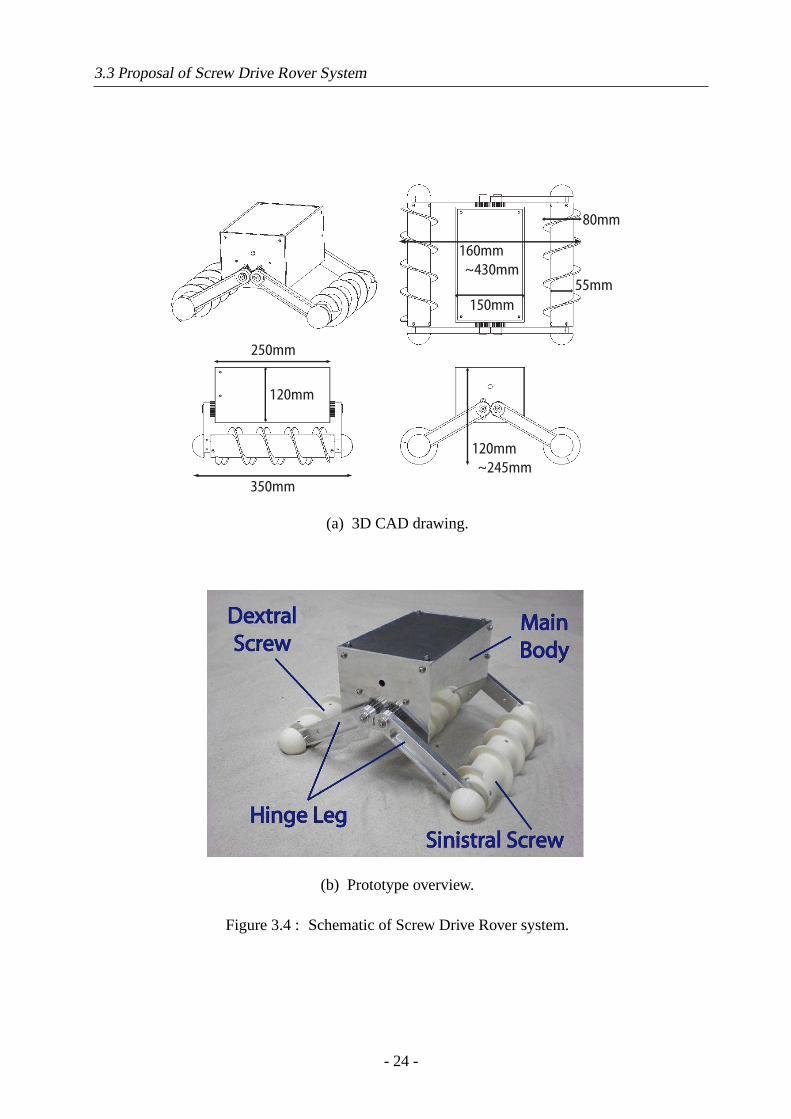
3.3 Proposal of Screw Drive Rover System
350mm
120mm
~245mm
80mm
55mm
150mm
120mm
250mm
160mm
~430mm
(a) 3D CAD drawing.
(b) Prototype overview.
Figure 3.4 : Schematic of Screw Drive Rover system.
- 24 -
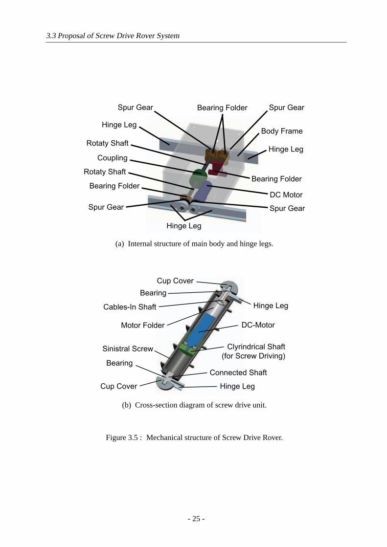
3.3 Proposal of Screw Drive Rover System
Body Frame
Spur Gear
Hinge Leg
Bearing Folder
Bearing Folder
Coupling
Hinge Leg
DC Motor
Spur Gear
Rotaty Shaft
Hinge Leg
Bearing Folder
Rotaty Shaft
Spur GearSpur Gear
(a) Internal structure of main body and hinge legs.
DC-Motor
Cables-In Shaft
Bearing
Cup Cover
Clyrindrical Shaft
(for Screw Driving)Sinistral Screw
Cup Cover
Bearing
Connected Shaft
Hinge Leg
Hinge Leg
Motor Folder
(b) Cross-section diagram of screw drive unit.
Figure 3.5 : Mechanical structure of Screw Drive Rover.
- 25 -
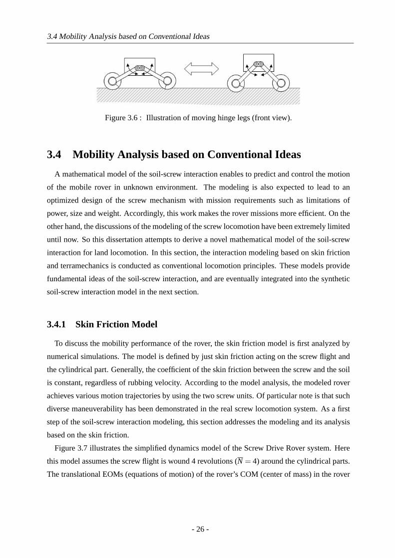
3.4 Mobility Analysis based on Conventional Ideas
Figure 3.6 : Illustration of moving hinge legs (front view).
3.4 Mobility Analysis based on Conventional Ideas
A mathematical model of the soil-screw interaction enables to predict and control the motion
of the mobile rover in unknown environment. The modeling is also expected to lead to an
optimized design of the screw mechanism with mission requirements such as limitations of
power, size and weight. Accordingly, this work makes the rover missions more efficient. On the
other hand, the discussions of the modeling of the screw locomotion have been extremely limited
until now. So this dissertation attempts to derive a novel mathematical model of the soil-screw
interaction for land locomotion. In this section, the interaction modeling based on skin friction
and terramechanics is conducted as conventional locomotion principles. These models provide
fundamental ideas of the soil-screw interaction, and are eventually integrated into the synthetic
soil-screw interaction model in the next section.
3.4.1 Skin Friction Model
To discuss the mobility performance of the rover, the skin friction model is first analyzed by
numerical simulations. The model is defined by just skin friction acting on the screw flight and
the cylindrical part. Generally, the coefficient of the skin friction between the screw and the soil
is constant, regardless of rubbing velocity. According to the model analysis, the modeled rover
achieves various motion trajectories by using the two screw units. Of particular note is that such
diverse maneuverability has been demonstrated in the real screw locomotion system. As a first
step of the soil-screw interaction modeling, this section addresses the modeling and its analysis
based on the skin friction.
Figure 3.7 illustrates the simplified dynamics model of the Screw Drive Rover system. Here
this model assumes the screw flight is wound4 revolutions (N = 4) around the cylindrical parts.
The translational EOMs (equations of motion) of the rover’s COM (center of mass) in the rover
- 26 -
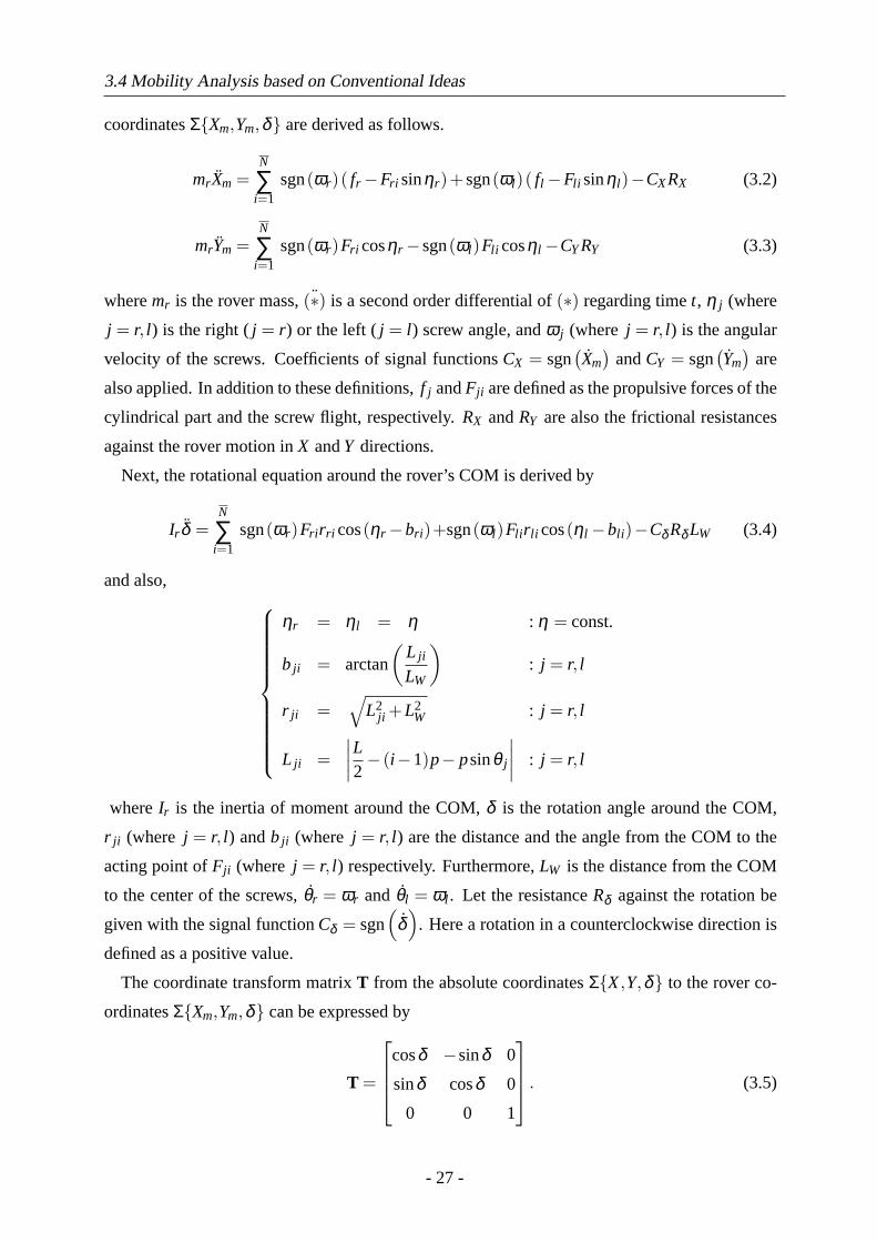
3.4 Mobility Analysis based on Conventional Ideas
coordinatesΣ{Xm,Ym,δ} are derived as follows.
mr Xm =N
∑i=1
sgn(ωr)( fr −Fri sinηr)+sgn(ωl )( fl −Fli sinηl )−CXRX (3.2)
mrYm =N
∑i=1
sgn(ωr)Fri cosηr −sgn(ωl )Fli cosηl −CYRY (3.3)
wheremr is the rover mass,(∗) is a second order differential of(∗) regarding timet, η j (where
j = r, l ) is the right (j = r) or the left (j = l ) screw angle, andω j (where j = r, l ) is the angular
velocity of the screws. Coefficients of signal functionsCX = sgn(Xm
)andCY = sgn
(Ym
)are
also applied. In addition to these definitions,f j andFji are defined as the propulsive forces of the
cylindrical part and the screw flight, respectively.RX andRY are also the frictional resistances
against the rover motion inX andY directions.
Next, the rotational equation around the rover’s COM is derived by
Ir δ =N
∑i=1
sgn(ωr)Fri rri cos(ηr −bri )+sgn(ωl )Fli r li cos(ηl −bli )−Cδ Rδ LW (3.4)
and also,
ηr = ηl = η : η = const.
b ji = arctan
(L ji
LW
): j = r, l
r ji =√
L2ji +L2
W : j = r, l
L ji =∣∣∣∣L2− (i−1)p− psinθ j
∣∣∣∣ : j = r, l
whereIr is the inertia of moment around the COM,δ is the rotation angle around the COM,
r ji (where j = r, l ) andb ji (where j = r, l ) are the distance and the angle from the COM to the
acting point ofFji (where j = r, l ) respectively. Furthermore,LW is the distance from the COM
to the center of the screws,θr = ωr and θl = ωl . Let the resistanceRδ against the rotation be
given with the signal functionCδ = sgn(
δ)
. Here a rotation in a counterclockwise direction is
defined as a positive value.
The coordinate transform matrixT from the absolute coordinatesΣ{X,Y,δ} to the rover co-
ordinatesΣ{Xm,Ym,δ} can be expressed by
T =
cosδ −sinδ 0
sinδ cosδ 0
0 0 1
. (3.5)
- 27 -
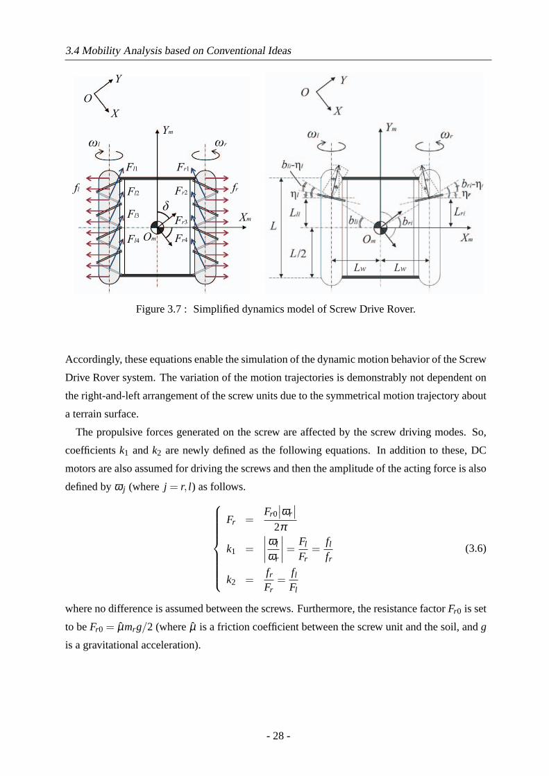
3.4 Mobility Analysis based on Conventional Ideas
Xm
Ym
ωrωl
Y
X
frfl
Fl1 Fr1
Fl2
Fl3
Fl4 Fr4
Fr2
Fr3
O
Om
δ
Lw Lw
Figure 3.7 : Simplified dynamics model of Screw Drive Rover.
Accordingly, these equations enable the simulation of the dynamic motion behavior of the Screw
Drive Rover system. The variation of the motion trajectories is demonstrably not dependent on
the right-and-left arrangement of the screw units due to the symmetrical motion trajectory about
a terrain surface.
The propulsive forces generated on the screw are affected by the screw driving modes. So,
coefficientsk1 andk2 are newly defined as the following equations. In addition to these, DC
motors are also assumed for driving the screws and then the amplitude of the acting force is also
defined byω j (where j = r, l ) as follows.
Fr =Fr0
∣∣ωr∣∣
2π
k1 =∣∣∣∣ωl
ωr
∣∣∣∣ =Fl
Fr=
flfr
k2 =frFr
=flFl
(3.6)
where no difference is assumed between the screws. Furthermore, the resistance factorFr0 is set
to beFr0 = µmrg/2 (whereµ is a friction coefficient between the screw unit and the soil, andg
is a gravitational acceleration).
- 28 -
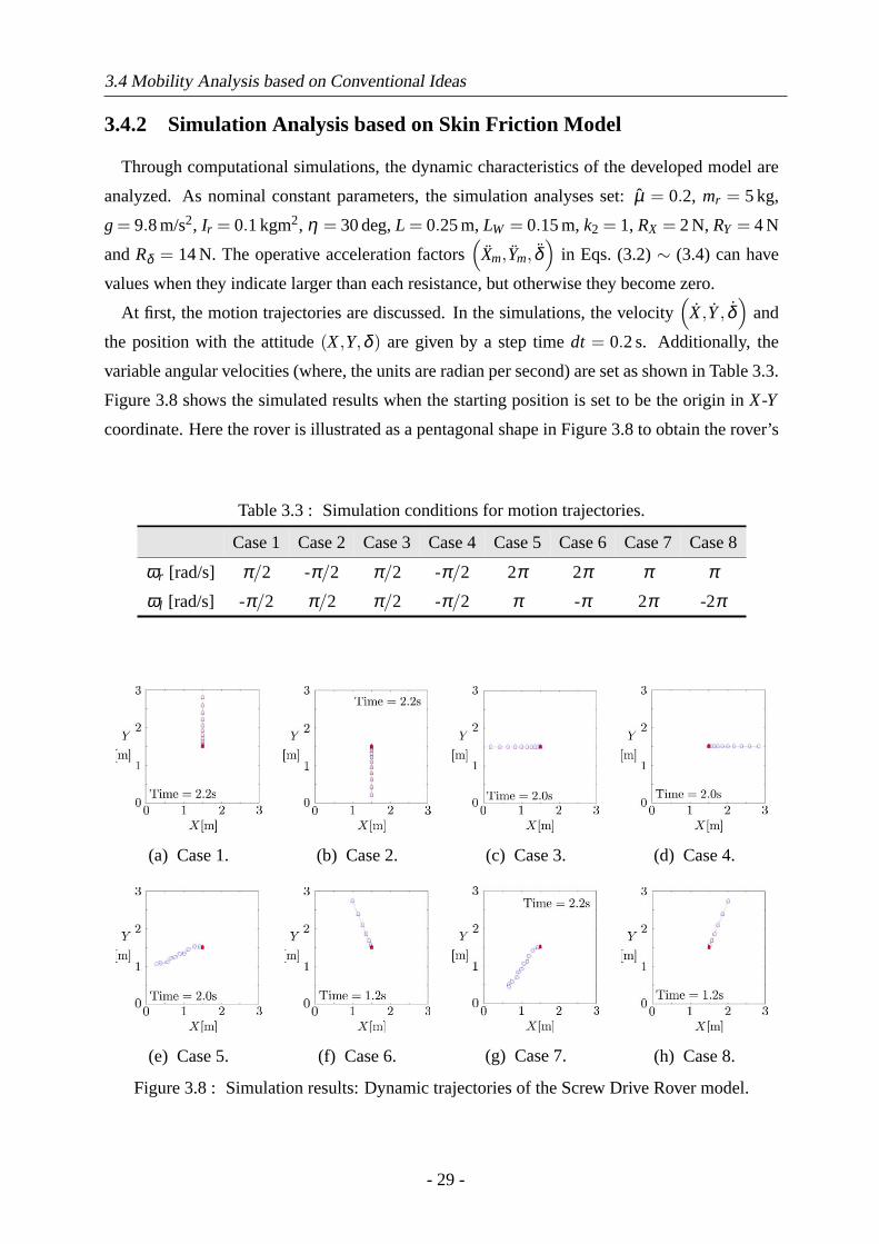
3.4 Mobility Analysis based on Conventional Ideas
3.4.2 Simulation Analysis based on Skin Friction Model
Through computational simulations, the dynamic characteristics of the developed model are
analyzed. As nominal constant parameters, the simulation analyses set:µ = 0.2, mr = 5kg,
g = 9.8m/s2, Ir = 0.1kgm2, η = 30deg,L = 0.25m, LW = 0.15m, k2 = 1, RX = 2N, RY = 4N
andRδ = 14N. The operative acceleration factors(
Xm,Ym, δ)
in Eqs. (3.2)∼ (3.4) can have
values when they indicate larger than each resistance, but otherwise they become zero.
At first, the motion trajectories are discussed. In the simulations, the velocity(
X,Y, δ)
and
the position with the attitude(X,Y,δ ) are given by a step timedt = 0.2s. Additionally, the
variable angular velocities (where, the units are radian per second) are set as shown in Table 3.3.
Figure 3.8 shows the simulated results when the starting position is set to be the origin inX-Y
coordinate. Here the rover is illustrated as a pentagonal shape in Figure 3.8 to obtain the rover’s
Table 3.3 : Simulation conditions for motion trajectories.
Case 1 Case 2 Case 3 Case 4 Case 5 Case 6 Case 7 Case 8
ωr [rad/s] π/2 -π/2 π/2 -π/2 2π 2π π πωl [rad/s] -π/2 π/2 π/2 -π/2 π -π 2π -2π
(a) Case 1. (b) Case 2. (c) Case 3. (d) Case 4.
(e) Case 5. (f) Case 6. (g) Case 7. (h) Case 8.
Figure 3.8 : Simulation results: Dynamic trajectories of the Screw Drive Rover model.
- 29 -
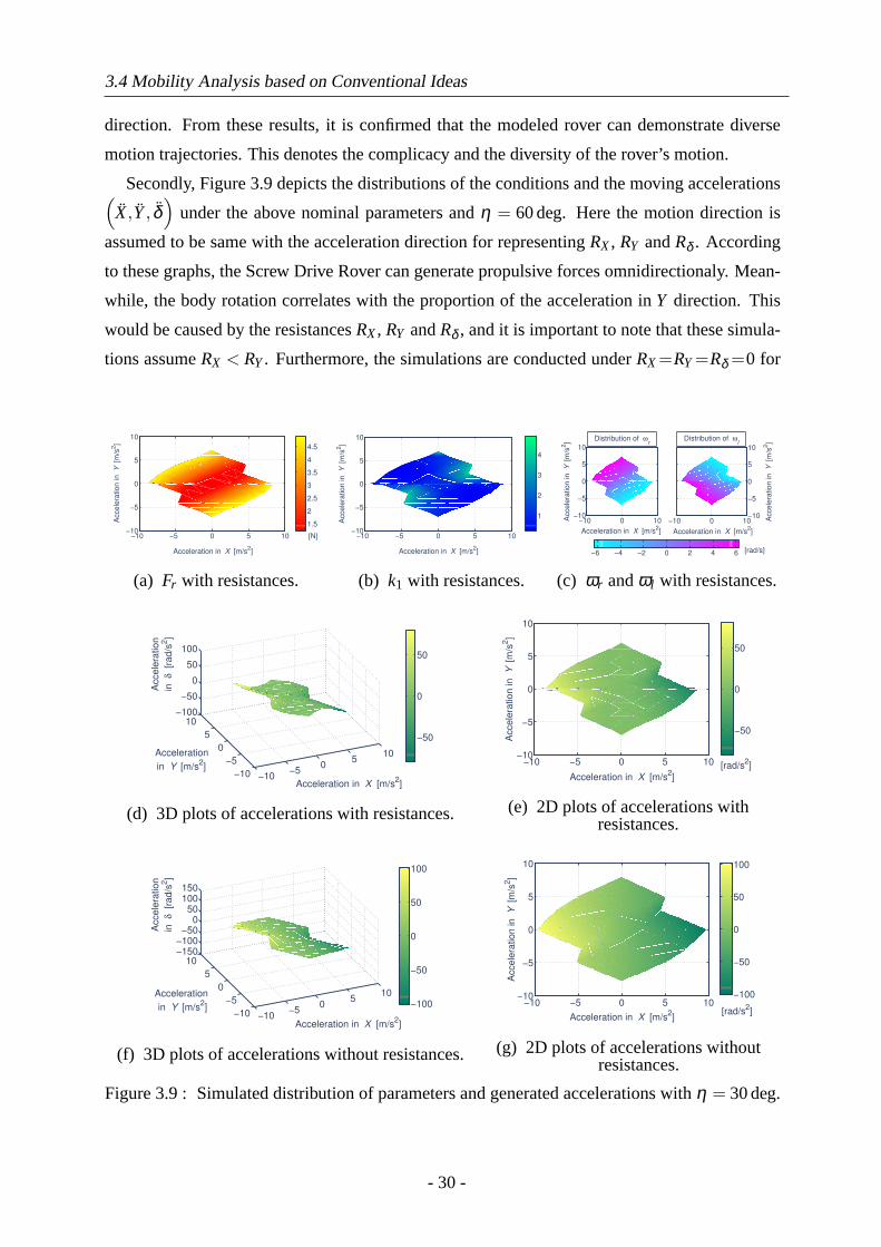
3.4 Mobility Analysis based on Conventional Ideas
direction. From these results, it is confirmed that the modeled rover can demonstrate diverse
motion trajectories. This denotes the complicacy and the diversity of the rover’s motion.
Secondly, Figure 3.9 depicts the distributions of the conditions and the moving accelerations(X,Y, δ
)under the above nominal parameters andη = 60deg. Here the motion direction is
assumed to be same with the acceleration direction for representingRX, RY andRδ . According
to these graphs, the Screw Drive Rover can generate propulsive forces omnidirectionaly. Mean-
while, the body rotation correlates with the proportion of the acceleration inY direction. This
would be caused by the resistancesRX, RY andRδ , and it is important to note that these simula-
tions assumeRX < RY. Furthermore, the simulations are conducted underRX =RY=Rδ =0 for
−10 −5 0 5 10−10
−5
0
5
10
Acceleration in X [m/s2]
Accele
ration in Y
[m
/s2]
1.5
2
2.5
3
3.5
4
4.5
[N]
(a) Fr with resistances.
−10 −5 0 5 10−10
−5
0
5
10
Acceleration in X [m/s2]
Accele
ration in Y
[m
/s2]
1
2
3
4
(b) k1 with resistances.
−10 0 10−10
−5
0
5
10
Acceleration in X [m/s2]
Accele
ration in Y
[m
/s2]
−10 0 10−10
−5
0
5
10
Accele
ration in Y
[m
/s2]
Acceleration in X [m/s2]
−6 −4 −2 0 2 4 6
Distribution of ωr
Distribution of ωl
[rad/s]
(c) ωr andωl with resistances.
−10−5
05
10
−10
−5
0
5
10
−100
−50
0
50
100
Acceleration in X [m/s2]
Acceleration
in Y [m/s2]
Acce
lera
tio
n
in
δ
[ra
d/s
2]
−50
0
50
(d) 3D plots of accelerations with resistances.
−10 −5 0 5 10−10
−5
0
5
10
Acceleration in X [m/s2]
Accele
ration in Y
[m
/s2]
−50
0
50
[rad/s2]
(e) 2D plots of accelerations withresistances.
−10−5
05
10
−10
−5
0
5
10
−150
−100
−50
0
50
100
150
Acceleration in X [m/s2]
Acceleration
in Y [m/s2]
Acce
lera
tio
n
in
δ
[ra
d/s
2]
−100
−50
0
50
100
(f) 3D plots of accelerations without resistances.
−10 −5 0 5 10−10
−5
0
5
10
Acceleration in X [m/s2]
Accele
ration in Y
[m
/s2]
−100
−50
0
50
100
[rad/s2]
(g) 2D plots of accelerations withoutresistances.
Figure 3.9 : Simulated distribution of parameters and generated accelerations withη = 30deg.
- 30 -
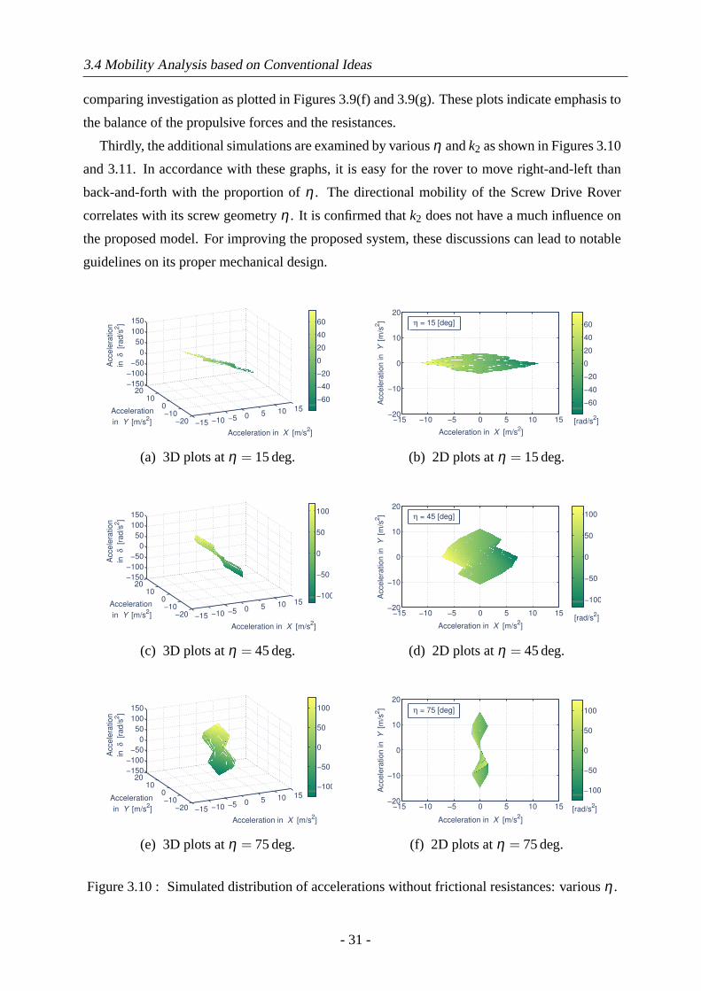
3.4 Mobility Analysis based on Conventional Ideas
comparing investigation as plotted in Figures 3.9(f) and 3.9(g). These plots indicate emphasis to
the balance of the propulsive forces and the resistances.
Thirdly, the additional simulations are examined by variousη andk2 as shown in Figures 3.10
and 3.11. In accordance with these graphs, it is easy for the rover to move right-and-left than
back-and-forth with the proportion ofη . The directional mobility of the Screw Drive Rover
correlates with its screw geometryη . It is confirmed thatk2 does not have a much influence on
the proposed model. For improving the proposed system, these discussions can lead to notable
guidelines on its proper mechanical design.
−15 −10 −5 0 5 10 15
−20
−10
0
10
20−150
−100
−50
0
50
100
150
Acceleration in X [m/s2]
Acceleration
in Y [m/s2]
Accele
ration
in
δ [r
ad/s
2]
−60
−40
−20
0
20
40
60
(a) 3D plots atη = 15deg.
−15 −10 −5 0 5 10 15−20
−10
0
10
20
Acceleration in X [m/s2]
Acce
lera
tio
n in
Y
[m
/s2]
−60
−40
−20
0
20
40
60η = 15 [deg]
[rad/s2]
(b) 2D plots atη = 15deg.
−15 −10 −5 0 5 10 15
−20
−10
0
10
20−150
−100
−50
0
50
100
150
Acceleration in X [m/s2]
Acceleration
in Y [m/s2]
Accele
ration
in
δ [r
ad/s
2]
−100
−50
0
50
100
(c) 3D plots atη = 45deg.
−15 −10 −5 0 5 10 15−20
−10
0
10
20
Acceleration in X [m/s2]
Accele
ration in Y
[m
/s2]
−100
−50
0
50
100η = 45 [deg]
[rad/s2]
(d) 2D plots atη = 45deg.
−15 −10 −5 0 5 10 15
−20
−10
0
10
20−150
−100
−50
0
50
100
150
Acceleration in X [m/s2]
Acceleration
in Y [m/s2]
Accele
ration
in
δ [r
ad/s
2]
−100
−50
0
50
100
(e) 3D plots atη = 75deg.
−15 −10 −5 0 5 10 15−20
−10
0
10
20
Acceleration in X [m/s2]
Accele
ration in Y
[m
/s2]
−100
−50
0
50
100
[rad/s2]
η = 75 [deg]
(f) 2D plots atη = 75deg.
Figure 3.10 : Simulated distribution of accelerations without frictional resistances: variousη .
- 31 -
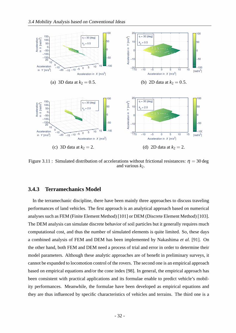
3.4 Mobility Analysis based on Conventional Ideas
−15 −10 −5 0 5 10 15
−20
−10
0
10
20−150
−100
−50
0
50
100
150
Acceleration in X [m/s2]
Acceleration
in Y [m/s2]
Accele
ration
in
δ [r
ad/s
2]
−100
−50
0
50
100
η = 30 [deg]
k2 = 0.5
(a) 3D data atk2 = 0.5.
−15 −10 −5 0 5 10 15−20
−10
0
10
20
Acceleration in X [m/s2]
Accele
ration in Y
[m
/s2]
−100
−50
0
50
100
[rad/s2]
η = 30 [deg]
k2 = 0.5
(b) 2D data atk2 = 0.5.
−15 −10 −5 0 5 10 15
−20
−10
0
10
20−150
−100
−50
0
50
100
150
Acceleration in X [m/s2]
Acceleration
in Y [m/s2]
Accele
ration
in
δ [r
ad/s
2]
−100
−50
0
50
100
η = 30 [deg]
k2 = 2.0
(c) 3D data atk2 = 2.
−15 −10 −5 0 5 10 15−20
−10
0
10
20
Acceleration in X [m/s2]
Accele
ration in Y
[m
/s2]
−100
−50
0
50
100
[rad/s2]
η = 30 [deg]
k2 = 2.0
(d) 2D data atk2 = 2.
Figure 3.11 : Simulated distribution of accelerations without frictional resistances:η = 30degand variousk2.
3.4.3 Terramechanics Model
In the terramechanic discipline, there have been mainly three approaches to discuss traveling
performances of land vehicles. The first approach is an analytical approach based on numerical
analyses such as FEM (Finite Element Method) [101] or DEM (Discrete Element Method) [103].
The DEM analysis can simulate discrete behavior of soil particles but it generally requires much
computational cost, and thus the number of simulated elements is quite limited. So, these days
a combined analysis of FEM and DEM has been implemented by Nakashimaet al. [91]. On
the other hand, both FEM and DEM need a process of trial and error in order to determine their
model parameters. Although these analytic approaches are of benefit in preliminary surveys, it
cannot be expanded to locomotion control of the rovers. The second one is an empirical approach
based on empirical equations and/or the cone index [98]. In general, the empirical approach has
been consistent with practical applications and its formulae enable to predict vehicle’s mobil-
ity performances. Meanwhile, the formulae have been developed as empirical equations and
they are thus influenced by specific characteristics of vehicles and terrains. The third one is a
- 32 -
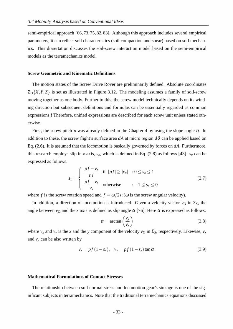
3.4 Mobility Analysis based on Conventional Ideas
semi-empirical approach [66, 73, 75, 82, 83]. Although this approach includes several empirical
parameters, it can reflect soil characteristics (soil compaction and shear) based on soil mechan-
ics. This dissertation discusses the soil-screw interaction model based on the semi-empirical
models as the terramechanics model.
Screw Geometric and Kinematic Definitions
The motion states of the Screw Drive Rover are preliminarily defined. Absolute coordinates
ΣO{X,Y,Z} is set as illustrated in Figure 3.12. The modeling assumes a family of soil-screw
moving together as one body. Further to this, the screw model technically depends on its wind-
ing direction but subsequent definitions and formulas can be essentially regarded as common
expressions.f Therefore, unified expressions are described for each screw unit unless stated oth-
erwise.
First, the screw pitchp was already defined in the Chapter 4 by using the slope angleη . In
addition to these, the screw flight’s surface areadA at micro regiondθ can be applied based on
Eq. (2.6). It is assumed that the locomotion is basically governed by forces ondA. Furthermore,
this research employs slip inx axis,sx, which is defined in Eq. (2.8) as follows [43].sx can be
expressed as follows.
sx =
p f−vx
p fif |p f | ≥ |vx| : 0≤ sx≤ 1
p f−vx
vxotherwise :−1≤ sx≤ 0
(3.7)
where f is the screw rotation speed andf = ω/2π (ω is the screw angular velocity).
In addition, a direction of locomotion is introduced. Given a velocity vectorvO in ΣS, the
angle betweenvO and thex axis is defined as slip angleα [76]. Hereα is expressed as follows.
α = arctan
(vy
vx
)(3.8)
wherevx andvy is thex and they component of the velocityvO in ΣS, respectively. Likewise,vx
andvy can be also written by
vx = p f (1−sx) , vy = p f (1−sx) tanα. (3.9)
Mathematical Formulations of Contact Stresses
The relationship between soil normal stress and locomotion gear’s sinkage is one of the sig-
nificant subjects in terramechanics. Note that the traditional terramechanics equations discussed
- 33 -
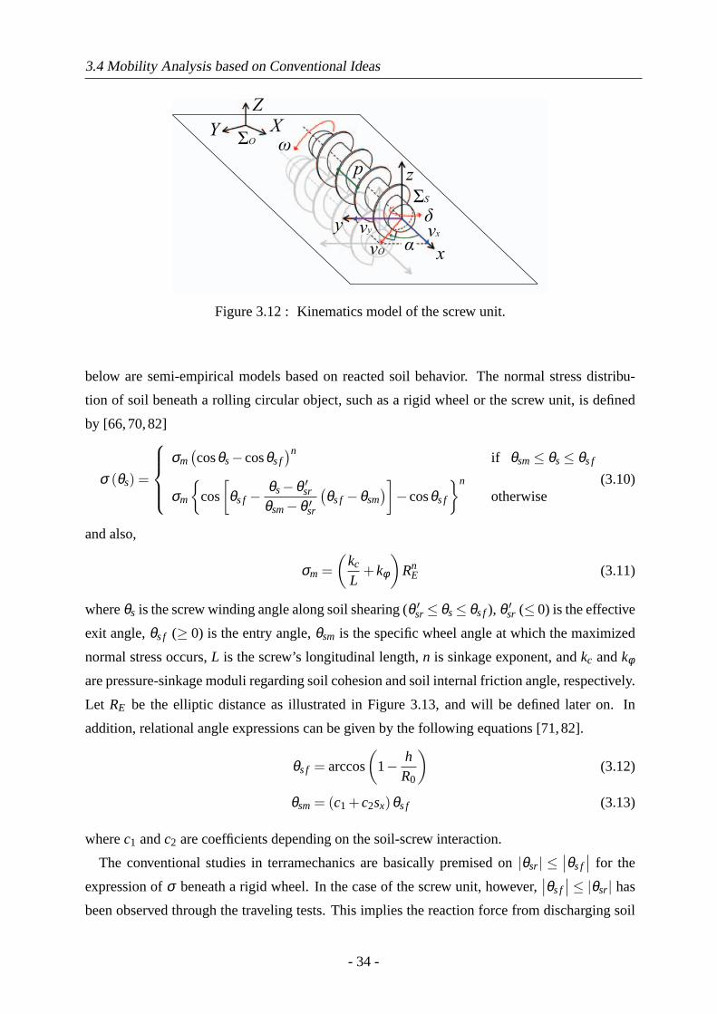
3.4 Mobility Analysis based on Conventional Ideas
ZXY
ΣO
ΣS
ω
vxvO x
y
z
δvy
α
p
Figure 3.12 : Kinematics model of the screw unit.
below are semi-empirical models based on reacted soil behavior. The normal stress distribu-
tion of soil beneath a rolling circular object, such as a rigid wheel or the screw unit, is defined
by [66,70,82]
σ (θs) =
σm(cosθs−cosθs f
)nif θsm≤ θs≤ θs f
σm
{cos
[θs f− θs−θ ′sr
θsm−θ ′sr
(θs f−θsm
)]−cosθs f
}n
otherwise(3.10)
and also,
σm =(
kc
L+kφ
)Rn
E (3.11)
whereθs is the screw winding angle along soil shearing (θ ′sr≤ θs≤ θs f), θ ′sr (≤ 0) is the effective
exit angle,θs f (≥ 0) is the entry angle,θsm is the specific wheel angle at which the maximized
normal stress occurs,L is the screw’s longitudinal length,n is sinkage exponent, andkc andkφ
are pressure-sinkage moduli regarding soil cohesion and soil internal friction angle, respectively.
Let RE be the elliptic distance as illustrated in Figure 3.13, and will be defined later on. In
addition, relational angle expressions can be given by the following equations [71,82].
θs f = arccos
(1− h
R0
)(3.12)
θsm= (c1 +c2sx)θs f (3.13)
wherec1 andc2 are coefficients depending on the soil-screw interaction.
The conventional studies in terramechanics are basically premised on|θsr| ≤∣∣θs f
∣∣ for the
expression ofσ beneath a rigid wheel. In the case of the screw unit, however,∣∣θs f
∣∣ ≤ |θsr| has
been observed through the traveling tests. This implies the reaction force from discharging soil
- 34 -
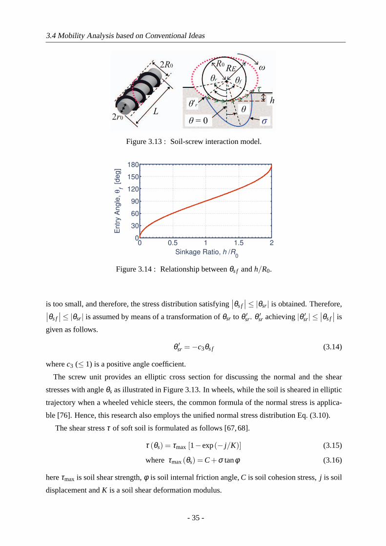
3.4 Mobility Analysis based on Conventional Ideas
L
R0RE ω
h
2r0
2R0
θθ’r
θr θf
θ = 0 σ
τ
Figure 3.13 : Soil-screw interaction model.
0 0.5 1 1.5 20
30
60
90
120
150
180
Sinkage Ratio, h /R0
En
try A
ng
le,
θf
[de
g]
Figure 3.14 : Relationship betweenθs f andh/R0.
is too small, and therefore, the stress distribution satisfying∣∣θs f
∣∣≤ |θsr| is obtained. Therefore,∣∣θs f∣∣≤ |θsr| is assumed by means of a transformation ofθsr to θ ′sr. θ ′sr achieving|θ ′sr| ≤
∣∣θs f∣∣ is
given as follows.
θ ′sr =−c3θs f (3.14)
wherec3 (≤ 1) is a positive angle coefficient.
The screw unit provides an elliptic cross section for discussing the normal and the shear
stresses with angleθs as illustrated in Figure 3.13. In wheels, while the soil is sheared in elliptic
trajectory when a wheeled vehicle steers, the common formula of the normal stress is applica-
ble [76]. Hence, this research also employs the unified normal stress distribution Eq. (3.10).
The shear stressτ of soft soil is formulated as follows [67,68].
τ (θs) = τmax [1−exp(− j/K)] (3.15)
where τmax(θs) = C+σ tanφ (3.16)
hereτmax is soil shear strength,φ is soil internal friction angle,C is soil cohesion stress,j is soil
displacement andK is a soil shear deformation modulus.
- 35 -
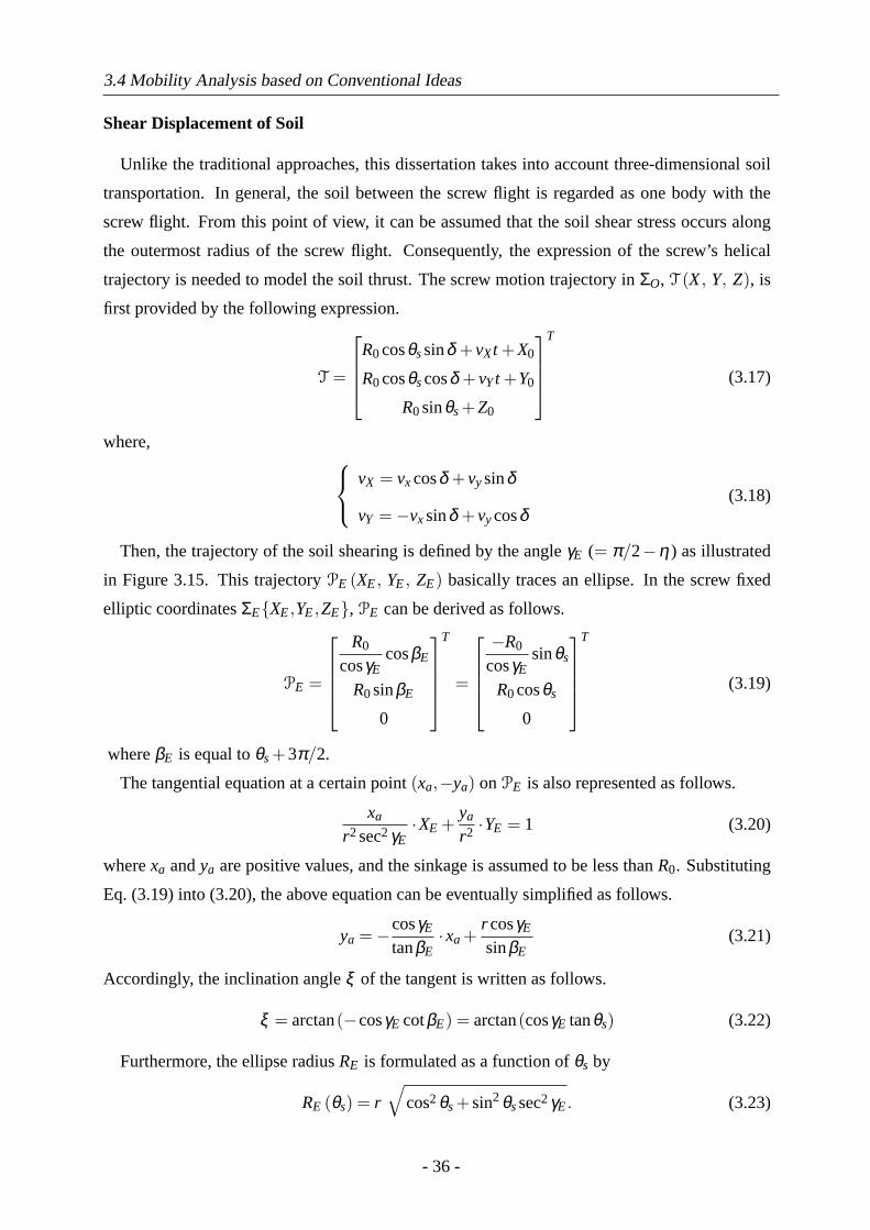
3.4 Mobility Analysis based on Conventional Ideas
Shear Displacement of Soil
Unlike the traditional approaches, this dissertation takes into account three-dimensional soil
transportation. In general, the soil between the screw flight is regarded as one body with the
screw flight. From this point of view, it can be assumed that the soil shear stress occurs along
the outermost radius of the screw flight. Consequently, the expression of the screw’s helical
trajectory is needed to model the soil thrust. The screw motion trajectory inΣO, T (X, Y, Z), is
first provided by the following expression.
T =
R0cosθssinδ +vXt +X0
R0cosθscosδ +vYt +Y0
R0sinθs+Z0
T
(3.17)
where,
vX = vxcosδ +vysinδ
vY =−vxsinδ +vycosδ(3.18)
Then, the trajectory of the soil shearing is defined by the angleγE (= π/2−η) as illustrated
in Figure 3.15. This trajectoryPE (XE, YE, ZE) basically traces an ellipse. In the screw fixed
elliptic coordinatesΣE{XE,YE,ZE}, PE can be derived as follows.
PE =
R0
cosγEcosβE
R0sinβE
0
T
=
−R0
cosγEsinθs
R0cosθs
0
T
(3.19)
whereβE is equal toθs+3π/2.
The tangential equation at a certain point(xa,−ya) onPE is also represented as follows.
xa
r2sec2γE·XE +
ya
r2 ·YE = 1 (3.20)
wherexa andya are positive values, and the sinkage is assumed to be less thanR0. Substituting
Eq. (3.19) into (3.20), the above equation can be eventually simplified as follows.
ya =−cosγE
tanβE·xa +
r cosγE
sinβE(3.21)
Accordingly, the inclination angleξ of the tangent is written as follows.
ξ = arctan(−cosγE cotβE) = arctan(cosγE tanθs) (3.22)
Furthermore, the ellipse radiusRE is formulated as a function ofθs by
RE (θs) = r√
cos2θs+sin2θssec2γE. (3.23)
- 36 -
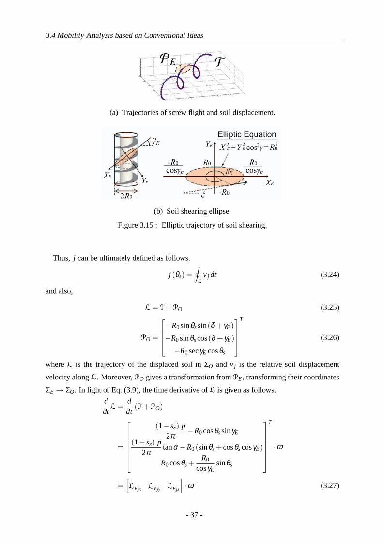
3.4 Mobility Analysis based on Conventional Ideas
(a) Trajectories of screw flight and soil displacement.
γ
YE
XE
XE
YE
Elliptic Equation
ξ
X E + Y E cos γ = R
β
-R0
cosγ cosγ
2 2 22
R0
0
R0
2R0-R0
E
EE E
(b) Soil shearing ellipse.
Figure 3.15 : Elliptic trajectory of soil shearing.
Thus, j can be ultimately defined as follows.
j (θs) =∮
Lv j dt (3.24)
and also,
L = T +PO (3.25)
PO =
−R0sinθssin(δ + γE)
−R0sinθscos(δ + γE)
−R0secγE cosθs
T
(3.26)
whereL is the trajectory of the displaced soil inΣO and v j is the relative soil displacement
velocity alongL. Moreover,PO gives a transformation fromPE, transforming their coordinates
ΣE → ΣO. In light of Eq. (3.9), the time derivative ofL is given as follows.
ddt
L =ddt
(T +PO)
=
(1−sx) p2π
−R0cosθssinγE
(1−sx) p2π
tanα−R0(sinθs+cosθscosγE)
R0cosθs+R0
cosγEsinθs
T
·ω
=[Lv jx Lv jy Lv jz
]·ω (3.27)
- 37 -
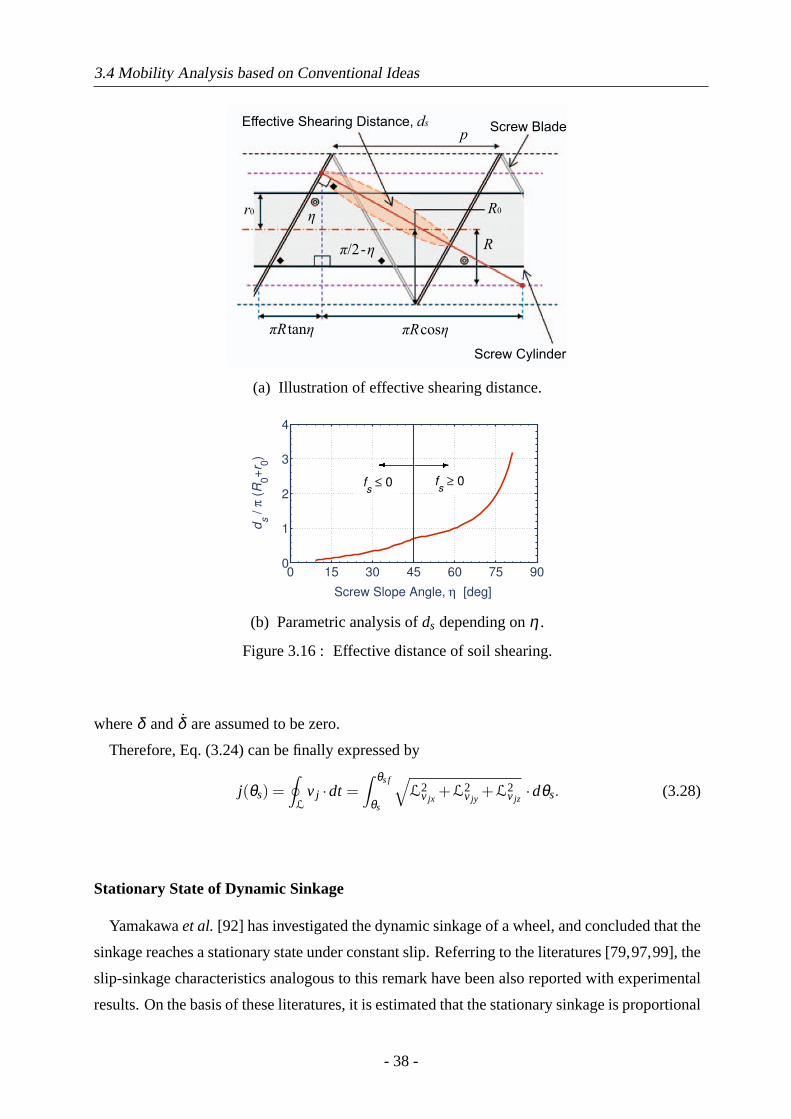
3.4 Mobility Analysis based on Conventional Ideas
Effective Shearing Distance, ds
Screw Cylinder
Screw Bladep
η
π/2 - η
πR cosη
r0
πR tanη
R
R0
(a) Illustration of effective shearing distance.
0 15 30 45 60 75 900
1
2
3
4
Screw Slope Angle, η [deg]
ds / π
(R
0+
r 0)
fs ≥ 0f
s ≤ 0
(b) Parametric analysis ofds depending onη .
Figure 3.16 : Effective distance of soil shearing.
whereδ andδ are assumed to be zero.
Therefore, Eq. (3.24) can be finally expressed by
j(θs) =∮
Lv j ·dt =
∫ θs f
θs
√L2
v jx+L2
v jy+L2
v jz·dθs. (3.28)
Stationary State of Dynamic Sinkage
Yamakawaet al. [92] has investigated the dynamic sinkage of a wheel, and concluded that the
sinkage reaches a stationary state under constant slip. Referring to the literatures [79,97,99], the
slip-sinkage characteristics analogous to this remark have been also reported with experimental
results. On the basis of these literatures, it is estimated that the stationary sinkage is proportional
- 38 -
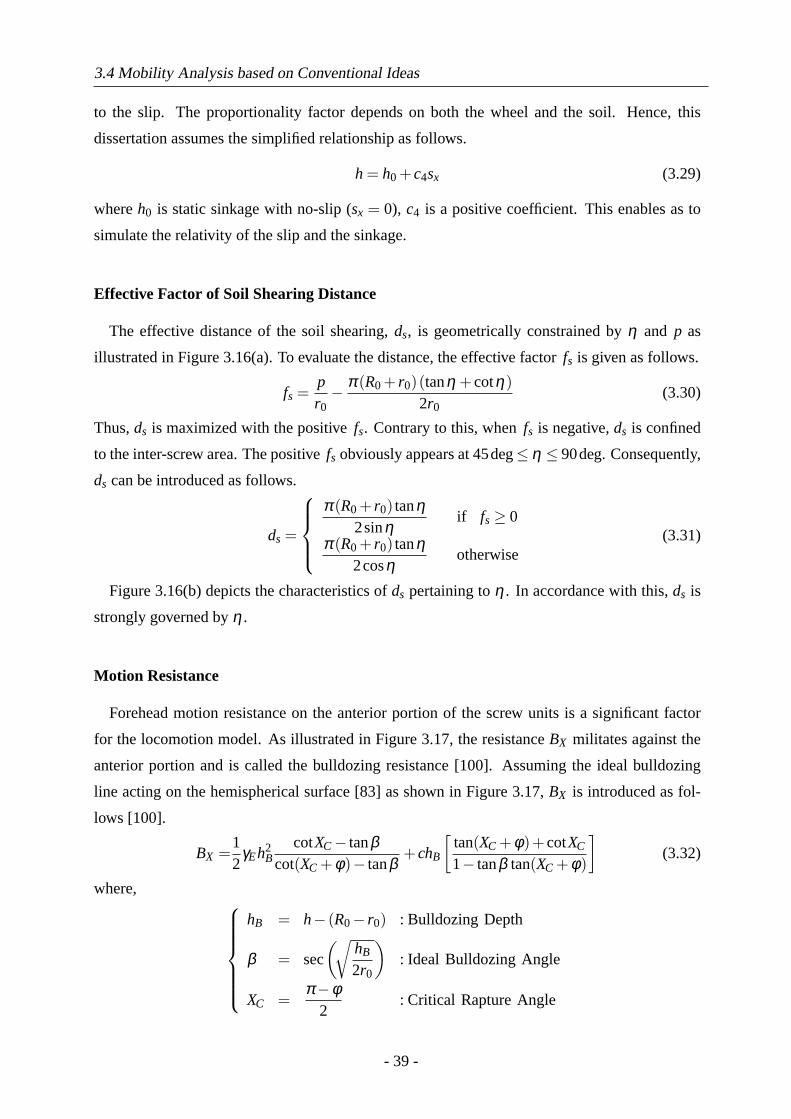
3.4 Mobility Analysis based on Conventional Ideas
to the slip. The proportionality factor depends on both the wheel and the soil. Hence, this
dissertation assumes the simplified relationship as follows.
h = h0 +c4sx (3.29)
whereh0 is static sinkage with no-slip (sx = 0), c4 is a positive coefficient. This enables as to
simulate the relativity of the slip and the sinkage.
Effective Factor of Soil Shearing Distance
The effective distance of the soil shearing,ds, is geometrically constrained byη and p as
illustrated in Figure 3.16(a). To evaluate the distance, the effective factorfs is given as follows.
fs =pr0− π (R0 + r0)(tanη +cotη)
2r0(3.30)
Thus,ds is maximized with the positivefs. Contrary to this, whenfs is negative,ds is confined
to the inter-screw area. The positivefs obviously appears at45deg≤ η ≤ 90deg. Consequently,
ds can be introduced as follows.
ds =
π (R0 + r0) tanη2sinη
if fs≥ 0
π (R0 + r0) tanη2cosη
otherwise(3.31)
Figure 3.16(b) depicts the characteristics ofds pertaining toη . In accordance with this,ds is
strongly governed byη .
Motion Resistance
Forehead motion resistance on the anterior portion of the screw units is a significant factor
for the locomotion model. As illustrated in Figure 3.17, the resistanceBX militates against the
anterior portion and is called the bulldozing resistance [100]. Assuming the ideal bulldozing
line acting on the hemispherical surface [83] as shown in Figure 3.17,BX is introduced as fol-
lows [100].
BX =12
γEh2B
cotXC− tanβcot(XC +φ)− tanβ
+chB
[tan(XC +φ)+cotXC
1− tanβ tan(XC +φ)
](3.32)
where,
hB = h− (R0− r0) : Bulldozing Depth
β = sec
(√hB
2r0
): Ideal Bulldozing Angle
XC =π−φ
2: Critical Rapture Angle
- 39 -
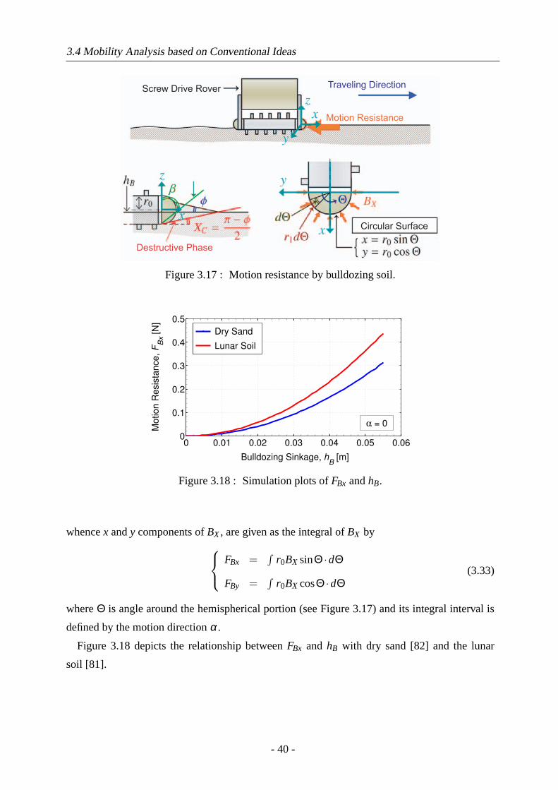
3.4 Mobility Analysis based on Conventional Ideas
Screw Drive Rover Traveling Direction
Destructive Phase
Circular Surface
Motion Resistance
Figure 3.17 : Motion resistance by bulldozing soil.
0 0.01 0.02 0.03 0.04 0.05 0.060
0.1
0.2
0.3
0.4
0.5
Bulldozing Sinkage, hB [m]
Mo
tio
n R
esis
tan
ce
, F
Bx [
N]
Dry Sand
Lunar Soil
α = 0
Figure 3.18 : Simulation plots ofFBx andhB.
whencex andy components ofBX, are given as the integral ofBX by
FBx =∫
r0BX sinΘ ·dΘ
FBy =∫
r0BX cosΘ ·dΘ(3.33)
whereΘ is angle around the hemispherical portion (see Figure 3.17) and its integral interval is
defined by the motion directionα.
Figure 3.18 depicts the relationship betweenFBx and hB with dry sand [82] and the lunar
soil [81].
- 40 -
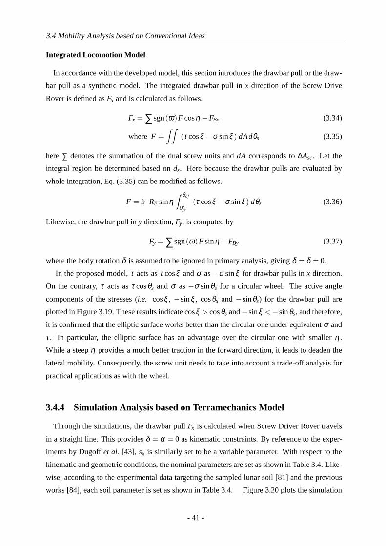
3.4 Mobility Analysis based on Conventional Ideas
Integrated Locomotion Model
In accordance with the developed model, this section introduces the drawbar pull or the draw-
bar pull as a synthetic model. The integrated drawbar pull inx direction of the Screw Drive
Rover is defined asFx and is calculated as follows.
Fx = ∑sgn(ω)F cosη−FBx (3.34)
where F =∫ ∫
(τ cosξ −σ sinξ ) dAdθs (3.35)
here∑ denotes the summation of the dual screw units anddA corresponds to∆Asc. Let the
integral region be determined based onds. Here because the drawbar pulls are evaluated by
whole integration, Eq. (3.35) can be modified as follows.
F = b·RE sinη∫ θs f
θ ′sr
(τ cosξ −σ sinξ ) dθs (3.36)
Likewise, the drawbar pull iny direction,Fy, is computed by
Fy = ∑sgn(ω)F sinη−FBy (3.37)
where the body rotationδ is assumed to be ignored in primary analysis, givingδ = δ = 0.
In the proposed model,τ acts asτ cosξ andσ as−σ sinξ for drawbar pulls inx direction.
On the contrary,τ acts asτ cosθs andσ as−σ sinθs for a circular wheel. The active angle
components of the stresses (i.e. cosξ , −sinξ , cosθs and−sinθs) for the drawbar pull are
plotted in Figure 3.19. These results indicatecosξ > cosθs and−sinξ <−sinθs, and therefore,
it is confirmed that the elliptic surface works better than the circular one under equivalentσ and
τ. In particular, the elliptic surface has an advantage over the circular one with smallerη .
While a steepη provides a much better traction in the forward direction, it leads to deaden the
lateral mobility. Consequently, the screw unit needs to take into account a trade-off analysis for
practical applications as with the wheel.
3.4.4 Simulation Analysis based on Terramechanics Model
Through the simulations, the drawbar pullFx is calculated when Screw Driver Rover travels
in a straight line. This providesδ = α = 0 as kinematic constraints. By reference to the exper-
iments by Dugoffet al. [43], sx is similarly set to be a variable parameter. With respect to the
kinematic and geometric conditions, the nominal parameters are set as shown in Table 3.4. Like-
wise, according to the experimental data targeting the sampled lunar soil [81] and the previous
works [84], each soil parameter is set as shown in Table 3.4. Figure 3.20 plots the simulation
- 41 -
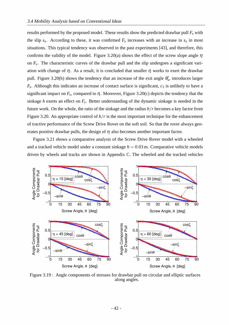
3.4 Mobility Analysis based on Conventional Ideas
results performed by the proposed model. These results show the predicted drawbar pullFx with
the slipsx. According to these, it was confirmedFx increases with an increase insx in most
situations. This typical tendency was observed in the past experiments [43], and therefore, this
confirms the validity of the model. Figure 3.20(a) shows the effect of the screw slope angleηon Fx. The characteristic curves of the drawbar pull and the slip undergoes a significant vari-
ation with change ofη . As a result, it is concluded that smallerη works to exert the drawbar
pull. Figure 3.20(b) shows the tendency that an increase of the exit angleθ ′sr introduces larger
Fx. Although this indicates an increase of contact surface is significant,c3 is unlikely to have a
significant impact onFx, compared toη . Moreover, Figure 3.20(c) depicts the tendency that the
sinkageh exerts an effect onFx. Better understanding of the dynamic sinkage is needed in the
future work. On the whole, the ratio of the sinkage and the radiush/r becomes a key factor from
Figure 3.20. An appropriate control ofh/r is the most important technique for the enhancement
of tractive performance of the Screw Drive Rover on the soft soil. So that the rover always gen-
erates positive drawbar pulls, the design ofη also becomes another important factor.
Figure 3.21 shows a comparative analysis of the Screw Drive Rover model with a wheeled
and a tracked vehicle model under a constant sinkageh = 0.03m. Comparative vehicle models
driven by wheels and tracks are shown in Appendix C. The wheeled and the tracked vehicles
0 15 30 45 60 75 90−1
−0.5
0
0.5
1
Screw Angle, θ [deg]
An
gle
Co
mp
on
en
ts
for
Dra
wb
ar
Pu
ll
cosξη = 15 [deg]cosθ
−sinθ
−sinξ
0 15 30 45 60 75 90−1
−0.5
0
0.5
1
Screw Angle, θ [deg]
An
gle
Co
mp
on
en
ts
for
Dra
wb
ar
Pu
ll
cosθ
−sinθ
−sinξ
cosξη = 30 [deg]
0 15 30 45 60 75 90−1
−0.5
0
0.5
1
An
gle
Co
mp
on
en
ts
for
Dra
wb
ar
Pu
ll
Screw Angle, θ [deg]
cosξ
cosθη = 45 [deg]
−sinθ
−sinξ
0 15 30 45 60 75 90−1
−0.5
0
0.5
1
Screw Angle, θ [deg]
An
gle
Co
mp
on
en
ts
for
Dra
wb
ar
Pu
ll
cosθη = 60 [deg]
−sinθ
−sinξ
cosξ
Figure 3.19 : Angle components of stresses for drawbar pull on circular and elliptic surfacesalong angles.
- 42 -
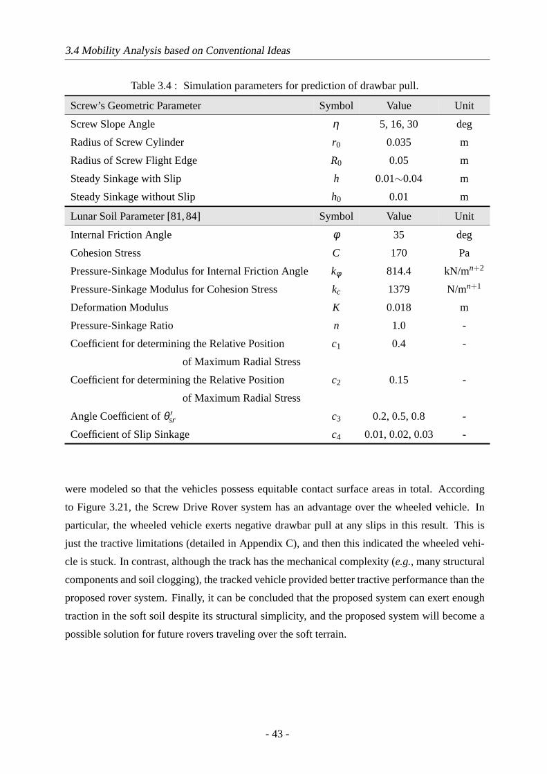
3.4 Mobility Analysis based on Conventional Ideas
Table 3.4 : Simulation parameters for prediction of drawbar pull.
Screw’s Geometric Parameter Symbol Value Unit
Screw Slope Angle η 5, 16, 30 deg
Radius of Screw Cylinder r0 0.035 m
Radius of Screw Flight Edge R0 0.05 m
Steady Sinkage with Slip h 0.01∼0.04 m
Steady Sinkage without Slip h0 0.01 m
Lunar Soil Parameter [81,84] Symbol Value Unit
Internal Friction Angle φ 35 deg
Cohesion Stress C 170 Pa
Pressure-Sinkage Modulus for Internal Friction Angle kφ 814.4 kN/mn+2
Pressure-Sinkage Modulus for Cohesion Stress kc 1379 N/mn+1
Deformation Modulus K 0.018 m
Pressure-Sinkage Ratio n 1.0 -
Coefficient for determining the Relative Position c1 0.4 -
of Maximum Radial Stress
Coefficient for determining the Relative Position c2 0.15 -
of Maximum Radial Stress
Angle Coefficient ofθ ′sr c3 0.2, 0.5, 0.8 -
Coefficient of Slip Sinkage c4 0.01, 0.02, 0.03 -
were modeled so that the vehicles possess equitable contact surface areas in total. According
to Figure 3.21, the Screw Drive Rover system has an advantage over the wheeled vehicle. In
particular, the wheeled vehicle exerts negative drawbar pull at any slips in this result. This is
just the tractive limitations (detailed in Appendix C), and then this indicated the wheeled vehi-
cle is stuck. In contrast, although the track has the mechanical complexity (e.g., many structural
components and soil clogging), the tracked vehicle provided better tractive performance than the
proposed rover system. Finally, it can be concluded that the proposed system can exert enough
traction in the soft soil despite its structural simplicity, and the proposed system will become a
possible solution for future rovers traveling over the soft terrain.
- 43 -
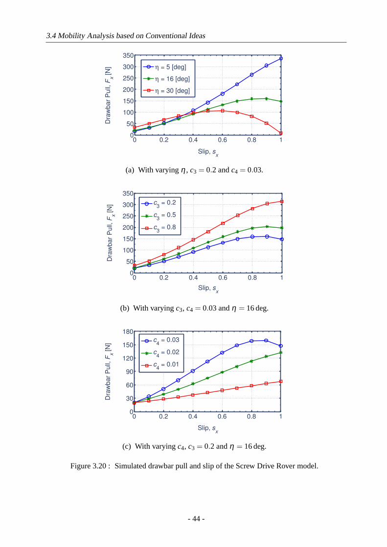
3.4 Mobility Analysis based on Conventional Ideas
0 0.2 0.4 0.6 0.8 10
50
100
150
200
250
300
350
Slip, sx
Dra
wb
ar
Pu
ll, F
x [
N]
η = 5 [deg]
η = 16 [deg]
η = 30 [deg]
(a) With varyingη , c3 = 0.2 andc4 = 0.03.
0 0.2 0.4 0.6 0.8 10
50
100
150
200
250
300
350
Dra
wb
ar
Pu
ll, F
x [
N]
Slip, sx
c3 = 0.2
c3 = 0.5
c3 = 0.8
(b) With varyingc3, c4 = 0.03andη = 16deg.
0 0.2 0.4 0.6 0.8 10
30
60
90
120
150
180
Slip, sx
Dra
wb
ar
Pu
ll, F
x [
N]
c4 = 0.03
c4 = 0.02
c4 = 0.01
(c) With varyingc4, c3 = 0.2 andη = 16deg.
Figure 3.20 : Simulated drawbar pull and slip of the Screw Drive Rover model.
- 44 -
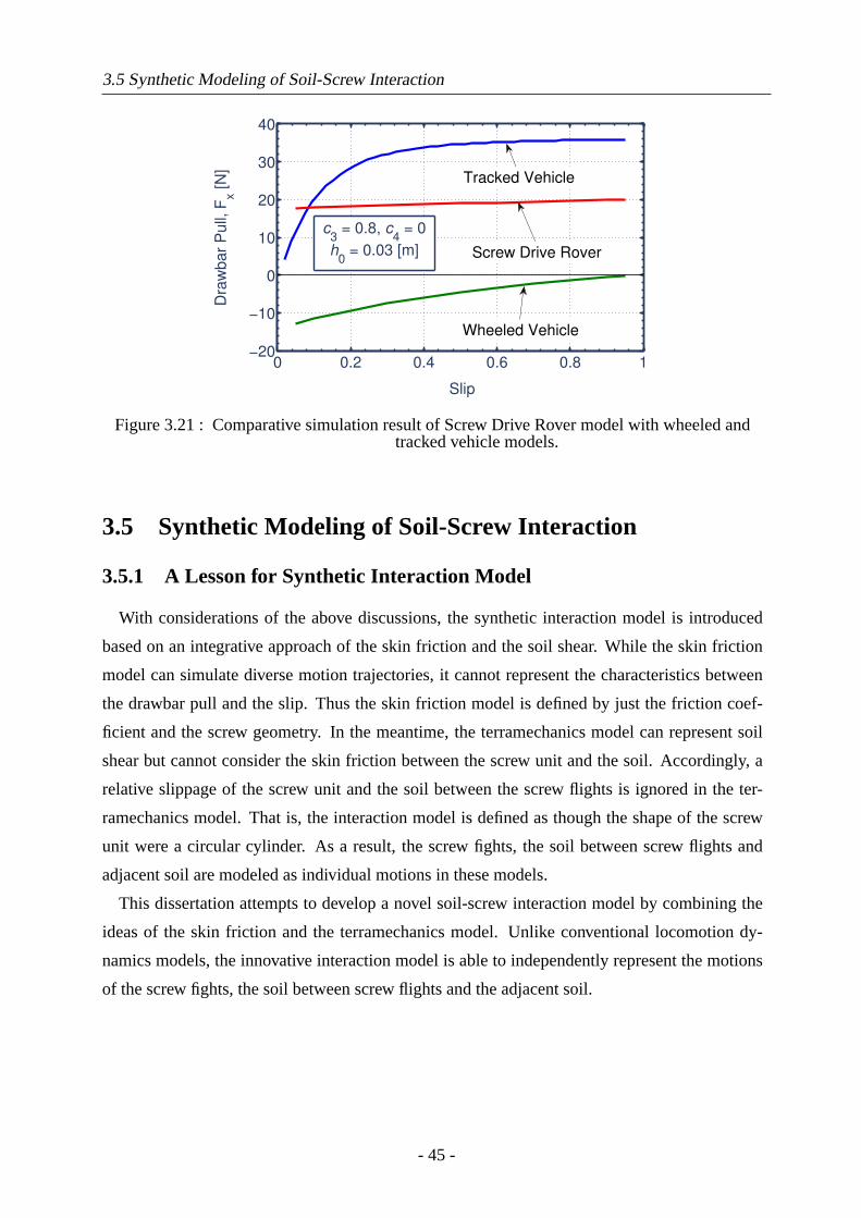
3.5 Synthetic Modeling of Soil-Screw Interaction
0 0.2 0.4 0.6 0.8 1−20
−10
0
10
20
30
40
Slip
Dra
wb
ar
Pu
ll, F
x [
N]
Wheeled Vehicle
Tracked Vehicle
Screw Drive Rover
c3 = 0.8, c
4 = 0
h0 = 0.03 [m]
Figure 3.21 : Comparative simulation result of Screw Drive Rover model with wheeled andtracked vehicle models.
3.5 Synthetic Modeling of Soil-Screw Interaction
3.5.1 A Lesson for Synthetic Interaction Model
With considerations of the above discussions, the synthetic interaction model is introduced
based on an integrative approach of the skin friction and the soil shear. While the skin friction
model can simulate diverse motion trajectories, it cannot represent the characteristics between
the drawbar pull and the slip. Thus the skin friction model is defined by just the friction coef-
ficient and the screw geometry. In the meantime, the terramechanics model can represent soil
shear but cannot consider the skin friction between the screw unit and the soil. Accordingly, a
relative slippage of the screw unit and the soil between the screw flights is ignored in the ter-
ramechanics model. That is, the interaction model is defined as though the shape of the screw
unit were a circular cylinder. As a result, the screw fights, the soil between screw flights and
adjacent soil are modeled as individual motions in these models.
This dissertation attempts to develop a novel soil-screw interaction model by combining the
ideas of the skin friction and the terramechanics model. Unlike conventional locomotion dy-
namics models, the innovative interaction model is able to independently represent the motions
of the screw fights, the soil between screw flights and the adjacent soil.
- 45 -
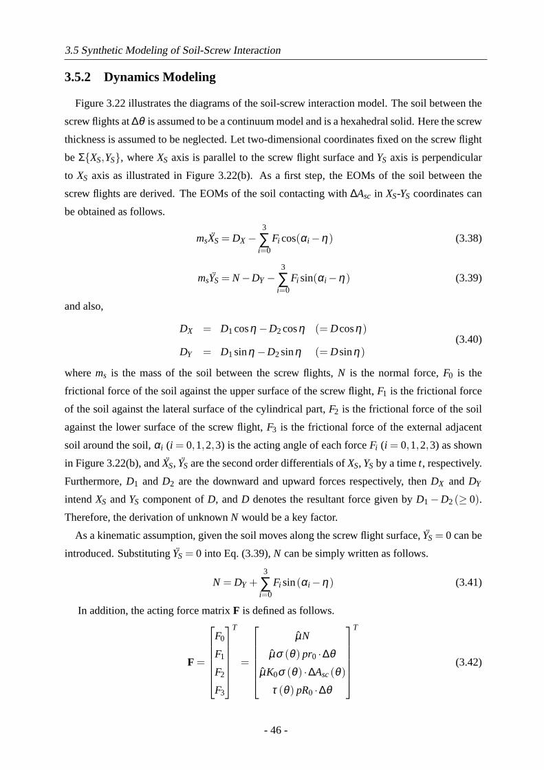
3.5 Synthetic Modeling of Soil-Screw Interaction
3.5.2 Dynamics Modeling
Figure 3.22 illustrates the diagrams of the soil-screw interaction model. The soil between the
screw flights at∆θ is assumed to be a continuum model and is a hexahedral solid. Here the screw
thickness is assumed to be neglected. Let two-dimensional coordinates fixed on the screw flight
be Σ{XS,YS}, whereXS axis is parallel to the screw flight surface andYS axis is perpendicular
to XS axis as illustrated in Figure 3.22(b). As a first step, the EOMs of the soil between the
screw flights are derived. The EOMs of the soil contacting with∆Asc in XS-YS coordinates can
be obtained as follows.
msXS = DX−3
∑i=0
Fi cos(αi−η) (3.38)
msYS = N−DY−3
∑i=0
Fi sin(αi−η) (3.39)
and also,
DX = D1cosη−D2cosη (= Dcosη)
DY = D1sinη−D2sinη (= Dsinη)(3.40)
wherems is the mass of the soil between the screw flights,N is the normal force,F0 is the
frictional force of the soil against the upper surface of the screw flight,F1 is the frictional force
of the soil against the lateral surface of the cylindrical part,F2 is the frictional force of the soil
against the lower surface of the screw flight,F3 is the frictional force of the external adjacent
soil around the soil,αi (i = 0,1,2,3) is the acting angle of each forceFi (i = 0,1,2,3) as shown
in Figure 3.22(b), andXS, YS are the second order differentials ofXS, YS by a timet, respectively.
Furthermore,D1 andD2 are the downward and upward forces respectively, thenDX andDY
intendXS andYS component ofD, andD denotes the resultant force given byD1−D2(≥ 0).
Therefore, the derivation of unknownN would be a key factor.
As a kinematic assumption, given the soil moves along the screw flight surface,YS= 0 can be
introduced. SubstitutingYS = 0 into Eq. (3.39),N can be simply written as follows.
N = DY +3
∑i=0
Fi sin(αi−η) (3.41)
In addition, the acting force matrixF is defined as follows.
F =
F0
F1
F2
F3
T
=
µN
µσ (θ) pr0 ·∆θµK0σ (θ) ·∆Asc(θ)
τ (θ) pR0 ·∆θ
T
(3.42)
- 46 -
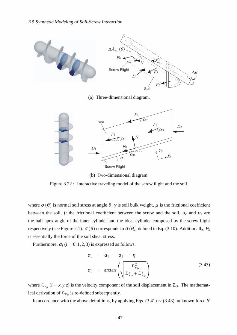
3.5 Synthetic Modeling of Soil-Screw Interaction
N
F0
F2
F3
F1
D1
Screw Flight
Soil
(a) Three-dimensional diagram.
XS
YS
N
F0
F2
F3
F1
D1
D2
0
3
2
1
Screw Flight
Soil
(b) Two-dimensional diagram.
Figure 3.22 : Interactive traveling model of the screw flight and the soil.
whereσ (θ) is normal soil stress at angleθ , γ is soil bulk weight,µ is the frictional coefficient
between the soil,µ the frictional coefficient between the screw and the soil,αc and αs are
the half apex angle of the inner cylinder and the ideal cylinder composed by the screw flight
respectively (see Figure 2.1).σ (θ) corresponds toσ (θs) defined in Eq. (3.10). Additionally,F3
is essentially the force of the soil shear stress.
Furthermore,αi (i = 0,1,2,3) is expressed as follows.
α0 = α1 = α2 = η
α3 = arctan
√√√√ L2v jx
L2v jy
+L2v jz
(3.43)
whereLv ji (i = x,y,z) is the velocity component of the soil displacement inΣO. The mathemat-
ical derivation ofLv ji is re-defined subsequently.
In accordance with the above definitions, by applying Eqs. (3.41)∼ (3.43), unknown forceN
- 47 -
3.5 Synthetic Modeling of Soil-Screw Interaction
can be definitely obtained by
N = Dsinη +F3sin(α3−η) . (3.44)
As the next step, the resultant forceD is introduced. In this dissertation, the soil is assumed
to be transported with a constant speed. Based upon this assumption,XS becomes zero, and
therefore,D can be given by applying Eq. (3.39) as follows.
D =F0 +F1 +F2 +F3cos(α3−η)
cosη(3.45)
The soil displacementj defined in Eq. (3.28) is applied to calculateτ. But, because the skin
friction occurs and the soil moves along the screw flight surface,Lv ji (wherei = x,y,z) defined
in Eq. (3.27) needs to be rewritten as follows.
Lv jx
Lv jy
Lv jz
T
=
sxp2π
R0cosθs+tanα2π
p(1−sx)
R0sinθs
T
·c5 (3.46)
wherec5 is a soil transportation factor, and body angleδ is also assumed to be zero.
Accordingly, the drawbar pulls inx andy directions are calculated as follows.
Fx = ∑∫ θ=2Nπ
θ=0
(Ncosη−
2
∑i=0
Fi sinαi
)−FBX (3.47)
Fy = ∑∫ θ=2Nπ
θ=0
[2
∑i=0
(Fi cosαi +Nsinη)cosθ − r0pσ sinξ ·dθ
]−FBY (3.48)
where the second term on the right-hand side of Eq. (3.48),r0pσ sinξdθ , militates against the
rover’s locomotion as soil compaction resistance.
Likewise, the total frictional resistance momentMT exerted by the soil between the screw
flights can be calculated as follows.
MT =∫ θ=2Nπ
θ=0(∆MN +∆MF) (3.49)
and also,
∆MN = NRsinη (3.50)
∆MF = F · r (3.51)
r =[Rcosα0 r0cosα1 Rcosα2 0
]T(3.52)
wherer is the coefficient matrix ofF for converting into torques.
- 48 -
3.6 Summary
3.5.3 Simulation Analysis
Based upon the proposed synthetic model, parametric analyses are discussed by numerical
simulations. Figure 3.23 depicts a simulated characteristic between the drawbar pull and the
slip. The simulation conditions were assumed to be the lunar soil shown in Table 3.4. From this
result, it is confirmed that the drawbar pull is proportional to the slip under constant sinkage.
That is, this means a larger tractive drag provides a larger slip.
Furthermore, Figure 3.23(b) shows the comparative results of the Screw Drive Rover model
and a wheeled vehicle under constant contact area. The simulation conditions were selected to
simulate a wheel’s tractive limitations (see Appendix B). While the wheeled vehicle does not
exert positive traction with any slips, the Screw Drive Rover model can exert positive traction.
According to this, the Screw Drive Rover has an advantage over the wheeled vehicle in soft soil.
3.6 Summary
This chapter presented the mathematical models of the soil-screw interaction based on the skin
friction and terramechanics. These established models are critical elements for representing the
actual interaction. On the basis of these ideas, the novel synthetic model was proposed. As
the remarkable conclusions of the proposed model, the key remarks are simply summarized as
follows:
• To develop the soil-screw interaction model, both skin friction and soil shear phenomena
are combined.
• In the proposed model, the behaviors of the screw and the soil between the screw flights
are defined as individual motions respectively.
• Compaction and shear characteristic of the soil is also included.
• Relationship between the screw geometry and the tractive performance can be quantita-
tively evaluated.
- 49 -
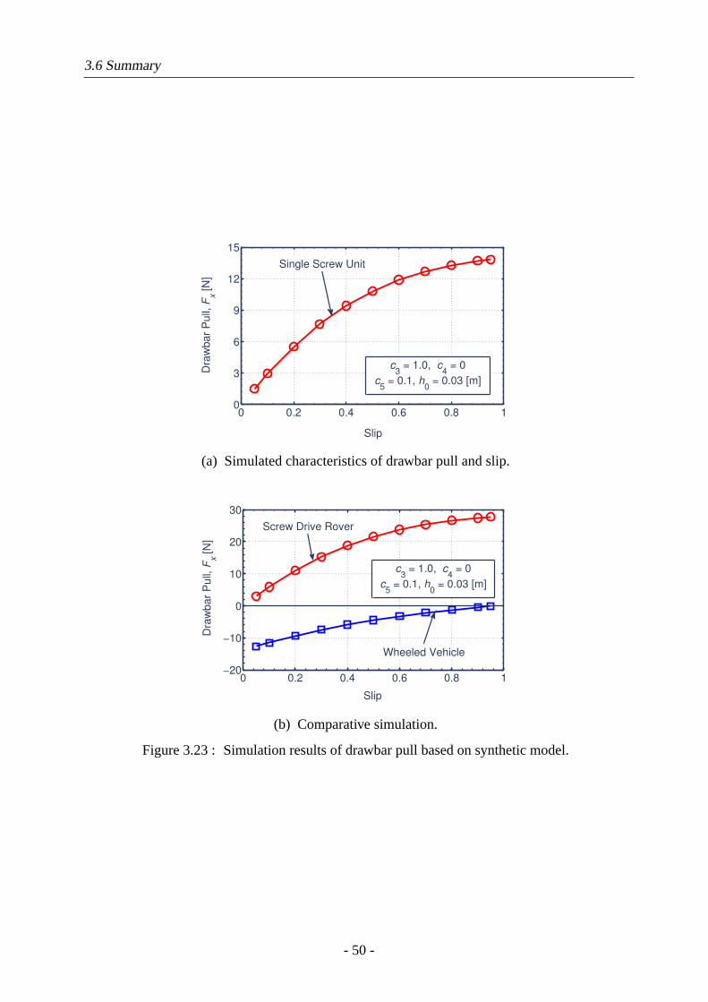
3.6 Summary
0 0.2 0.4 0.6 0.8 10
3
6
9
12
15
Slip
Dra
wb
ar
Pu
ll, F
x [
N]
c3 = 1.0, c
4 = 0
c5 = 0.1, h
0 = 0.03 [m]
Single Screw Unit
(a) Simulated characteristics of drawbar pull and slip.
0 0.2 0.4 0.6 0.8 1−20
−10
0
10
20
30
Slip
Dra
wb
ar
Pu
ll, F
x [
N]
Wheeled Vehicle
c3 = 1.0, c
4 = 0
c5 = 0.1, h
0 = 0.03 [m]
Screw Drive Rover
(b) Comparative simulation.
Figure 3.23 : Simulation results of drawbar pull based on synthetic model.
- 50 -
Chapter 4. Experimental Characteristics
of Screw Surface Locomotion
4.1 Trafficability Tests of Archimedean Screw Unit
4.1.1 Laboratory Test Environment
Figure 4.1 illustrates the schematic of an experimental system. Load acting on the screw unit
can be controlled by load canceler attached at the apex portion of the parallel-link. In general,
propulsion behavior of the unit is achieved by only thrust produced in the screw part, and trac-
tive drag is thus applied to the unit through a pulley. Consequently, the tractive characteristics
in various slip conditions can be investigated by changes in the tractive drag. The unit rotates
through the timing belt connected to a motor, and rotational speed of the unit can be controlled
based upon the motor’s encoder pulse. A steering motor is also embedded in order to inclined
the unit to the traveling direction. In this apparatus, rotational angles and currents of the motors,
traveling distance and sinkage can be measured throughout the tests. Considering uncertainty
and reproducibility of the tests on sand, several tests should be conducted in each condition.
Thus the resulted slip was evaluated as an average value with its error range. Schematic of the
screw unit is shown in Figure 4.2.
An overview of the actual experimental apparatus is shown in Figure 4.3. The sand box
(150×20×15 cm) is filled with quartz sand (no.5) and is same with the soil used in the ma-
neuverability experiments. The sand distributes in narrow range as shown in Figure 4.4, and is
thus basically weakly-compressible. Consequently, the quartz sand is regarded as a relatively-
reproducible sand for any physical tests.
4.1.2 Evaluation Scheme
Key Indexes
Key evaluation indexes in the traveling tests are first described. As screw geometric parame-
ters, the screw slope angleη and the screw pitchp in Eq. (2.4) are applied. These parameters are
- 51 -
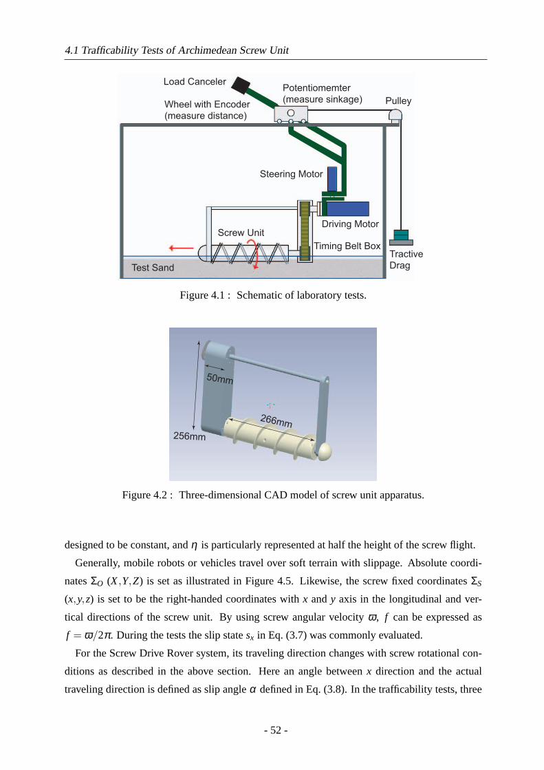
4.1 Trafficability Tests of Archimedean Screw Unit
Screw Unit
Load Canceler
Tractive
Drag
Pulley
Driving Motor
Steering Motor
Timing Belt Box
Test Sand
Potentiomemter
(measure sinkage)Wheel with Encoder
(measure distance)
Figure 4.1 : Schematic of laboratory tests.
50mm
266mm
256mm
Figure 4.2 : Three-dimensional CAD model of screw unit apparatus.
designed to be constant, andη is particularly represented at half the height of the screw flight.
Generally, mobile robots or vehicles travel over soft terrain with slippage. Absolute coordi-
natesΣO (X,Y,Z) is set as illustrated in Figure 4.5. Likewise, the screw fixed coordinatesΣS
(x,y,z) is set to be the right-handed coordinates withx andy axis in the longitudinal and ver-
tical directions of the screw unit. By using screw angular velocityω, f can be expressed as
f = ω/2π. During the tests the slip statesx in Eq. (3.7) was commonly evaluated.
For the Screw Drive Rover system, its traveling direction changes with screw rotational con-
ditions as described in the above section. Here an angle betweenx direction and the actual
traveling direction is defined as slip angleα defined in Eq. (3.8). In the trafficability tests, three
- 52 -
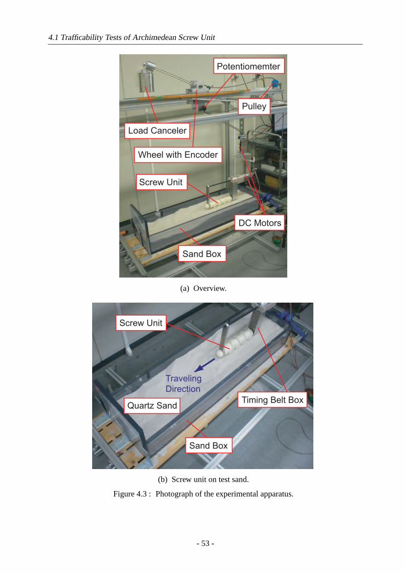
4.1 Trafficability Tests of Archimedean Screw Unit
Screw Unit
Load Canceler
DC Motors
Potentiomemter
Pulley
Sand Box
Wheel with Encoder
(a) Overview.
Screw Unit
Sand Box
Quartz SandTiming Belt Box
Traveling
Direction
(b) Screw unit on test sand.
Figure 4.3 : Photograph of the experimental apparatus.
- 53 -
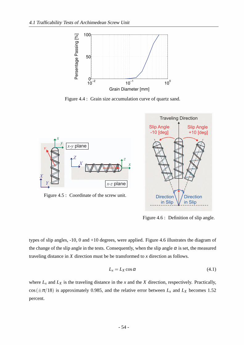
4.1 Trafficability Tests of Archimedean Screw Unit
10−2
10−1
100
0
50
100
Grain Diameter [mm]
Pers
enta
ge P
assin
g [%
]
Figure 4.4 : Grain size accumulation curve of quartz sand.
x
y
x
z
X
Y
v
v
X
Z
x-z plane
x-y plane
Figure 4.5 : Coordinate of the screw unit.
Traveling Direction
Slip Angle
+10 [deg]
Slip Angle
-10 [deg]
Direction
in Slip
Direction
in Slip
Figure 4.6 : Definition of slip angle.
types of slip angles, -10, 0 and +10 degrees, were applied. Figure 4.6 illustrates the diagram of
the change of the slip angle in the tests. Consequently, when the slip angleα is set, the measured
traveling distance inX direction must be be transformed tox direction as follows.
Lx = LX cosα (4.1)
whereLx andLX is the traveling distance in thex and theX direction, respectively. Practically,
cos(±π/18) is approximately 0.985, and the relative error betweenLx andLX becomes 1.52
percent.
- 54 -
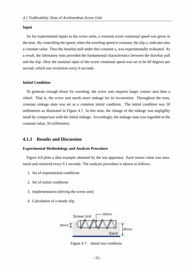
4.1 Trafficability Tests of Archimedean Screw Unit
Input
As for experimental inputs to the screw units, a constant screw rotational speed was given in
the tests. By controlling the speed, when the traveling speed is constant, the slipsx indicates also
a constant value. Thus the drawbar pull under this constantsx was experimentally evaluated. As
a result, the laboratory tests provided the fundamental characteristics between the drawbar pull
and the slip. Here the nominal input of the screw rotational speed was set to be 60 degrees per
second, which one revolution every 6 seconds.
Initial Condition
To generate enough thrust for traveling, the screw unit requires larger contact area than a
wheel. That is, the screw unit needs more sinkage for its locomotion. Throughout the tests,
constant sinkage state was set as a common initial condition. The initial condition was 50
millimeters as illustrated in Figure 4.7. In this tests, the change of the sinkage was negligibly
small by comparison with the initial sinkage. Accordingly, the sinkage state was regarded as the
constant value, 50 millimeters.
4.1.3 Results and Discussion
Experimental Methodology and Analysis Procedure
Figure 4.8 plots a data example obtained by the test apparatus. Each sensor value was mea-
sured and retrieved every 0.1 seconds. The analysis procedure is shown as follows:
1. Set of experimental conditions
2. Set of initial conditions
3. Implementation (driving the screw unit)
4. Calculation of a steady slip
85mm
50mm
55mm
Sand
Screw Unit
Figure 4.7 : Initial test condition.
- 55 -
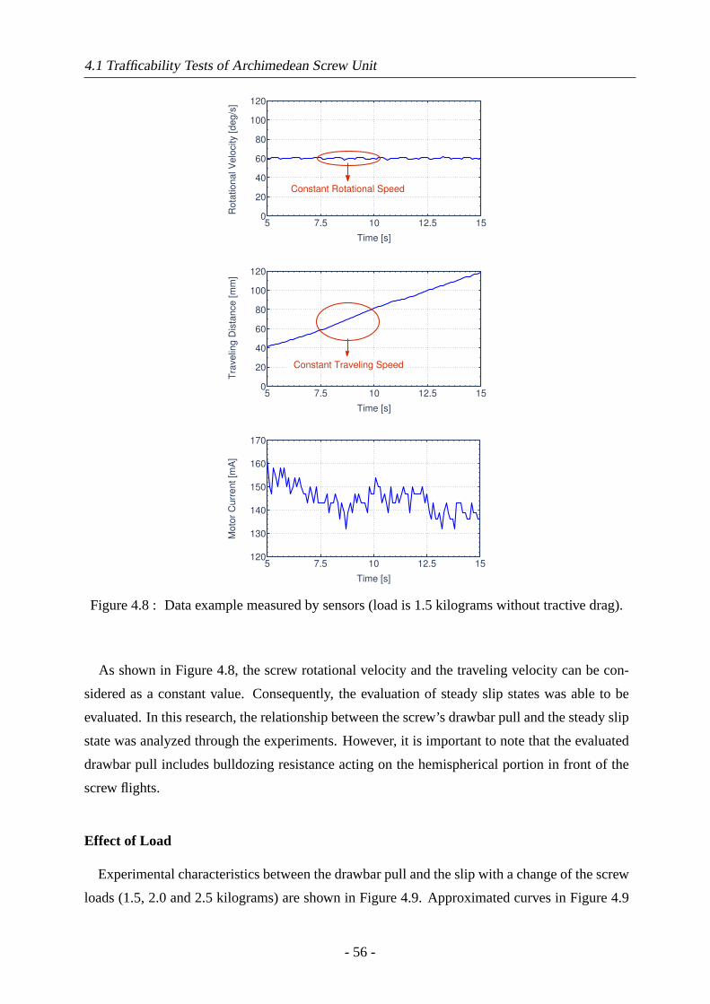
4.1 Trafficability Tests of Archimedean Screw Unit
5 7.5 10 12.5 150
20
40
60
80
100
120
Time [s]R
ota
tional V
elo
city [deg/s
]
Constant Rotational Speed
5 7.5 10 12.5 150
20
40
60
80
100
120
Time [s]
Tra
veling D
ista
nce [m
m]
Constant Traveling Speed
5 7.5 10 12.5 15120
130
140
150
160
170
Time [s]
Moto
r C
urr
ent [m
A]
Figure 4.8 : Data example measured by sensors (load is 1.5 kilograms without tractive drag).
As shown in Figure 4.8, the screw rotational velocity and the traveling velocity can be con-
sidered as a constant value. Consequently, the evaluation of steady slip states was able to be
evaluated. In this research, the relationship between the screw’s drawbar pull and the steady slip
state was analyzed through the experiments. However, it is important to note that the evaluated
drawbar pull includes bulldozing resistance acting on the hemispherical portion in front of the
screw flights.
Effect of Load
Experimental characteristics between the drawbar pull and the slip with a change of the screw
loads (1.5, 2.0 and 2.5 kilograms) are shown in Figure 4.9. Approximated curves in Figure 4.9
- 56 -
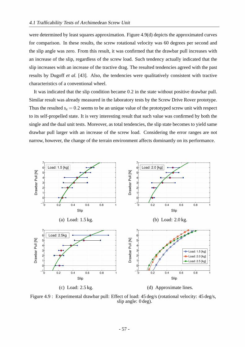
4.1 Trafficability Tests of Archimedean Screw Unit
were determined by least squares approximation. Figure 4.9(d) depicts the approximated curves
for comparison. In these results, the screw rotational velocity was 60 degrees per second and
the slip angle was zero. From this result, it was confirmed that the drawbar pull increases with
an increase of the slip, regardless of the screw load. Such tendency actually indicated that the
slip increases with an increase of the tractive drag. The resulted tendencies agreed with the past
results by Dugoffet al. [43]. Also, the tendencies were qualitatively consistent with tractive
characteristics of a conventional wheel.
It was indicated that the slip condition became0.2 in the state without positive drawbar pull.
Similar result was already measured in the laboratory tests by the Screw Drive Rover prototype.
Thus the resultedsx = 0.2 seems to be an unique value of the prototyped screw unit with respect
to its self-propelled state. It is very interesting result that such value was confirmed by both the
single and the dual unit tests. Moreover, as total tendencies, the slip state becomes to yield same
drawbar pull larger with an increase of the screw load. Considering the error ranges are not
narrow, however, the change of the terrain environment affects dominantly on its performance.
0 0.2 0.4 0.6 0.8 1−1
0
1
2
3
4
5
6
7
Slip
Dra
wb
ar
Pu
ll [
N]
Load: 1.5 [kg]
(a) Load: 1.5 kg.
0 0.2 0.4 0.6 0.8 1−1
0
1
2
3
4
5
6
7
Slip
Dra
wb
ar
Pu
ll [
N]
Load: 2.0 [kg]
(b) Load: 2.0 kg.
0 0.2 0.4 0.6 0.8 1−1
0
1
2
3
4
5
6
7
Slip
Dra
wbar
Pull [N
]
Load: 2.5kg
(c) Load: 2.5 kg.
0 0.2 0.4 0.6 0.8 1−1
0
1
2
3
4
5
6
7
Slip
Dra
wb
ar
Pu
ll [
N]
Load: 1.5 [kg]
Load: 2.0 [kg]
Load: 2.5 [kg]
(d) Approximate lines.
Figure 4.9 : Experimental drawbar pull: Effect of load: 45 deg/s (rotational velocity: 45 deg/s,slip angle: 0 deg).
- 57 -
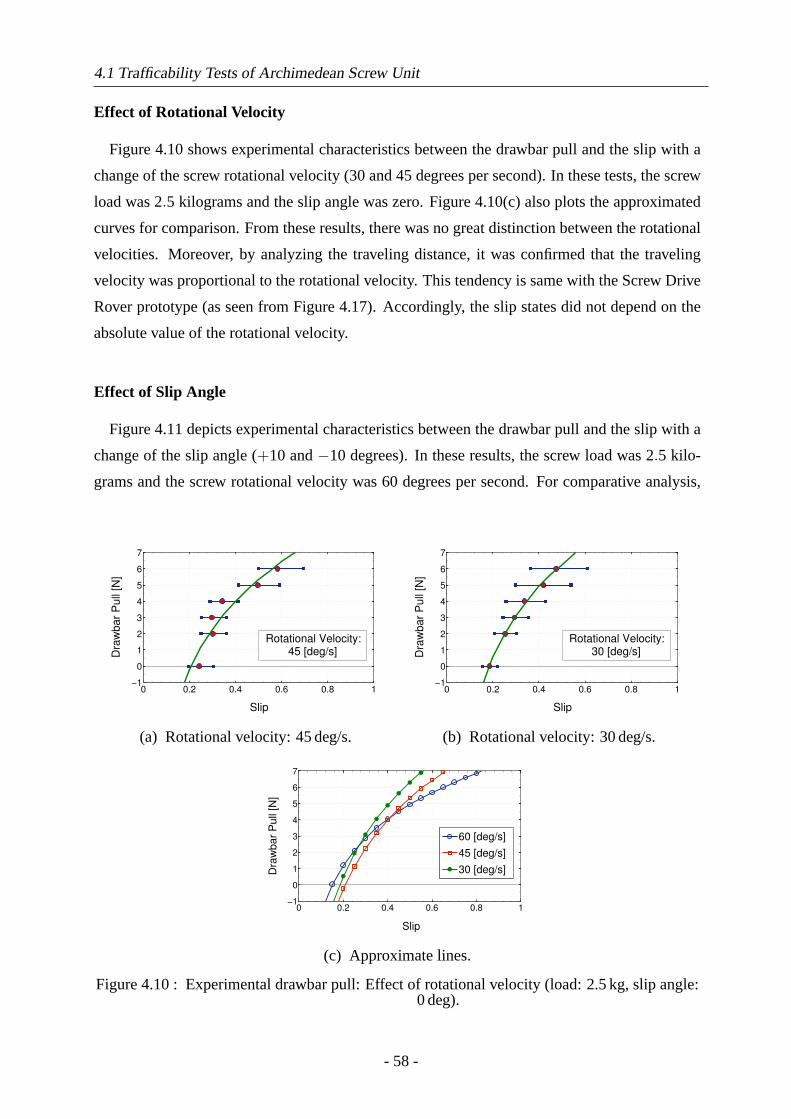
4.1 Trafficability Tests of Archimedean Screw Unit
Effect of Rotational Velocity
Figure 4.10 shows experimental characteristics between the drawbar pull and the slip with a
change of the screw rotational velocity (30and45degrees per second). In these tests, the screw
load was2.5 kilograms and the slip angle was zero. Figure 4.10(c) also plots the approximated
curves for comparison. From these results, there was no great distinction between the rotational
velocities. Moreover, by analyzing the traveling distance, it was confirmed that the traveling
velocity was proportional to the rotational velocity. This tendency is same with the Screw Drive
Rover prototype (as seen from Figure 4.17). Accordingly, the slip states did not depend on the
absolute value of the rotational velocity.
Effect of Slip Angle
Figure 4.11 depicts experimental characteristics between the drawbar pull and the slip with a
change of the slip angle (+10 and−10 degrees). In these results, the screw load was2.5 kilo-
grams and the screw rotational velocity was60 degrees per second. For comparative analysis,
0 0.2 0.4 0.6 0.8 1−1
0
1
2
3
4
5
6
7
Slip
Dra
wb
ar
Pu
ll [
N]
Rotational Velocity:
45 [deg/s]
(a) Rotational velocity: 45 deg/s.
0 0.2 0.4 0.6 0.8 1−1
0
1
2
3
4
5
6
7
Slip
Dra
wb
ar
Pu
ll [
N]
Rotational Velocity:
30 [deg/s]
(b) Rotational velocity: 30 deg/s.
0 0.2 0.4 0.6 0.8 1−1
0
1
2
3
4
5
6
7
Slip
Dra
wb
ar
Pu
ll [
N]
60 [deg/s]
45 [deg/s]
30 [deg/s]
(c) Approximate lines.
Figure 4.10 : Experimental drawbar pull: Effect of rotational velocity (load: 2.5 kg, slip angle:0 deg).
- 58 -
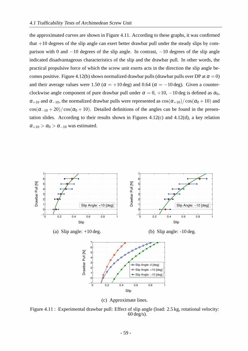
4.1 Trafficability Tests of Archimedean Screw Unit
the approximated curves are shown in Figure 4.11. According to these graphs, it was confirmed
that+10 degrees of the slip angle can exert better drawbar pull under the steady slips by com-
parison with0 and−10 degrees of the slip angle. In contrast,−10 degrees of the slip angle
indicated disadvantageous characteristics of the slip and the drawbar pull. In other words, the
practical propulsive force of which the screw unit exerts acts in the direction the slip angle be-
comes positive. Figure 4.12(b) shows normalized drawbar pulls (drawbar pulls over DP atα = 0)
and their average values were 1.50 (α = +10deg) and 0.64 (α = −10deg). Given a counter-
clockwise angle component of pure drawbar pull underα = 0, +10, −10deg is defined asα0,
α+10 andα−10, the normalized drawbar pulls were represented ascos(α+10)/cos(α0 +10) and
cos(α−10+ 20)/cos(α0 + 10). Detailed definitions of the angles can be found in the presen-
tation slides. According to their results shown in Figures 4.12(c) and 4.12(d), a key relation
α+10 > α0 > α−10 was estimated.
0 0.2 0.4 0.6 0.8 1−1
0
1
2
3
4
5
6
7
Slip
Dra
wb
ar
Pu
ll [
N]
Slip Angle: +10 [deg]
(a) Slip angle: +10 deg.
0 0.2 0.4 0.6 0.8 1−1
0
1
2
3
4
5
6
7
Slip
Dra
wb
ar
Pu
ll [
N]
Slip Angle: −10 [deg]
(b) Slip angle: -10 deg.
0 0.2 0.4 0.6 0.8 1−1
0
1
2
3
4
5
6
7
Slip
Dra
wb
ar
Pu
ll [
N]
Slip Angle: 0 [deg]
Slip Angle: +10 [deg]
Slip Angle: −10 [deg]
(c) Approximate lines.
Figure 4.11 : Experimental drawbar pull: Effect of slip angle (load: 2.5 kg, rotational velocity:60 deg/s).
- 59 -
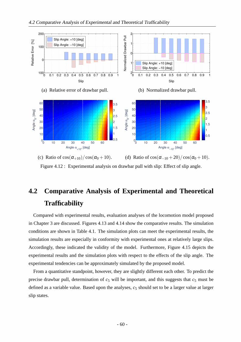
4.2 Comparative Analysis of Experimental and Theoretical Trafficability
0 0.1 0.2 0.3 0.4 0.5 0.6 0.7 0.8 0.9 1100
0
100
200
Slip
Rela
tive E
rror
[%
]
Slip Angle: +10 [deg]
Slip Angle: −10 [deg]
(a) Relative error of drawbar pull.
0 0.1 0.2 0.3 0.4 0.5 0.6 0.7 0.8 0.9 12
1
0
1
2
Slip
Norm
alized D
raw
bar
Pull
Slip Angle: +10 [deg]
Slip Angle: −10 [deg]
(b) Normalized drawbar pull.
0 10 20 30 40 50 600
10
20
30
40
50
60
Angle α+10
, [deg]
Angle
α0, [d
eg]
0.5
1
1.5
2
2.5
3
3.5
(c) Ratio ofcos(α+10)/cos(α0 +10).
0 10 20 30 40 50 600
10
20
30
40
50
60
Angle α−10
, [deg]
Angle
α0, [d
eg]
0.5
1
1.5
2
2.5
3
3.5
(d) Ratio ofcos(α−10+20)/cos(α0 +10).
Figure 4.12 : Experimental analysis on drawbar pull with slip: Effect of slip angle.
4.2 Comparative Analysis of Experimental and Theoretical
Trafficability
Compared with experimental results, evaluation analyses of the locomotion model proposed
in Chapter 3 are discussed. Figures 4.13 and 4.14 show the comparative results. The simulation
conditions are shown in Table 4.1. The simulation plots can meet the experimental results, the
simulation results are especially in conformity with experimental ones at relatively large slips.
Accordingly, these indicated the validity of the model. Furthermore, Figure 4.15 depicts the
experimental results and the simulation plots with respect to the effects of the slip angle. The
experimental tendencies can be approximately simulated by the proposed model.
From a quantitative standpoint, however, they are slightly different each other. To predict the
precise drawbar pull, determination ofc5 will be important, and this suggests thatc5 must be
defined as a variable value. Based upon the analyses,c5 should set to be a larger value at larger
slip states.
- 60 -
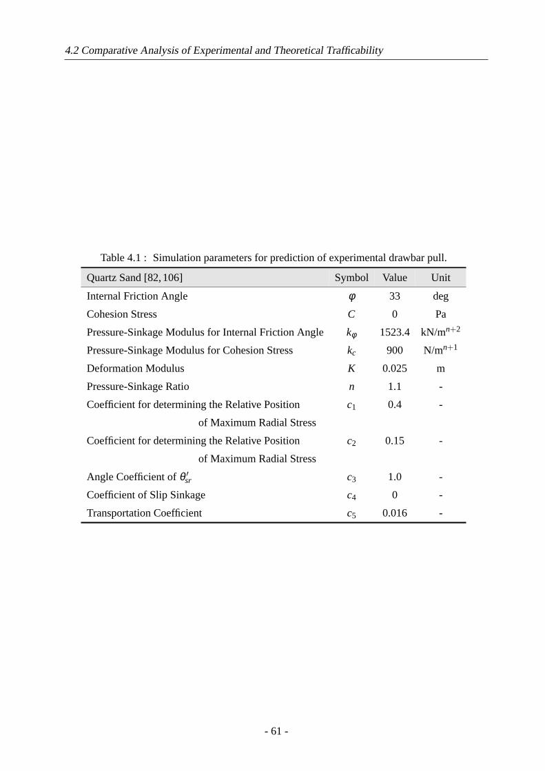
4.2 Comparative Analysis of Experimental and Theoretical Trafficability
Table 4.1 : Simulation parameters for prediction of experimental drawbar pull.
Quartz Sand [82,106] Symbol Value Unit
Internal Friction Angle φ 33 deg
Cohesion Stress C 0 Pa
Pressure-Sinkage Modulus for Internal Friction Angle kφ 1523.4 kN/mn+2
Pressure-Sinkage Modulus for Cohesion Stress kc 900 N/mn+1
Deformation Modulus K 0.025 m
Pressure-Sinkage Ratio n 1.1 -
Coefficient for determining the Relative Position c1 0.4 -
of Maximum Radial Stress
Coefficient for determining the Relative Position c2 0.15 -
of Maximum Radial Stress
Angle Coefficient ofθ ′sr c3 1.0 -
Coefficient of Slip Sinkage c4 0 -
Transportation Coefficient c5 0.016 -
- 61 -
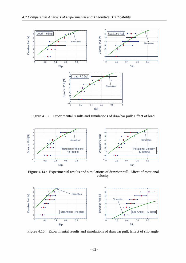
4.2 Comparative Analysis of Experimental and Theoretical Trafficability
0 0.2 0.4 0.6 0.8 1−1
0
1
2
3
4
5
6
7
Slip
Dra
wbar
Pull [N
]
Simulation
Load: 1.5 [kg]
0 0.2 0.4 0.6 0.8 1−1
0
1
2
3
4
5
6
7
Slip
Dra
wbar
Pull [N
]
Simulation
Load: 2.0 [kg]
0 0.2 0.4 0.6 0.8 1−1
0
1
2
3
4
5
6
7
Slip
Dra
wbar
Pull [N
]
Simulation
Load: 2.5 [kg]
Figure 4.13 : Experimental results and simulations of drawbar pull: Effect of load.
0 0.2 0.4 0.6 0.8 1−1
0
1
2
3
4
5
6
7
Slip
Dra
wbar
Pull [N
]
Rotational Velocity:
45 [deg/s]
Simulation
0 0.2 0.4 0.6 0.8 1−1
0
1
2
3
4
5
6
7
Slip
Dra
wbar
Pull [N
]
Rotational Velocity:
30 [deg/s]
Simulation
Figure 4.14 : Experimental results and simulations of drawbar pull: Effect of rotationalvelocity.
0 0.2 0.4 0.6 0.8 1−1
0
1
2
3
4
5
6
7
Slip
Dra
wbar
Pull [N
]
Slip Angle: +10 [deg]
Simulation
0 0.2 0.4 0.6 0.8 1−1
0
1
2
3
4
5
6
7
Slip
Dra
wbar
Pull [N
]
Slip Angle: −10 [deg]
Simulation
Figure 4.15 : Experimental results and simulations of drawbar pull: Effect of slip angle.
- 62 -
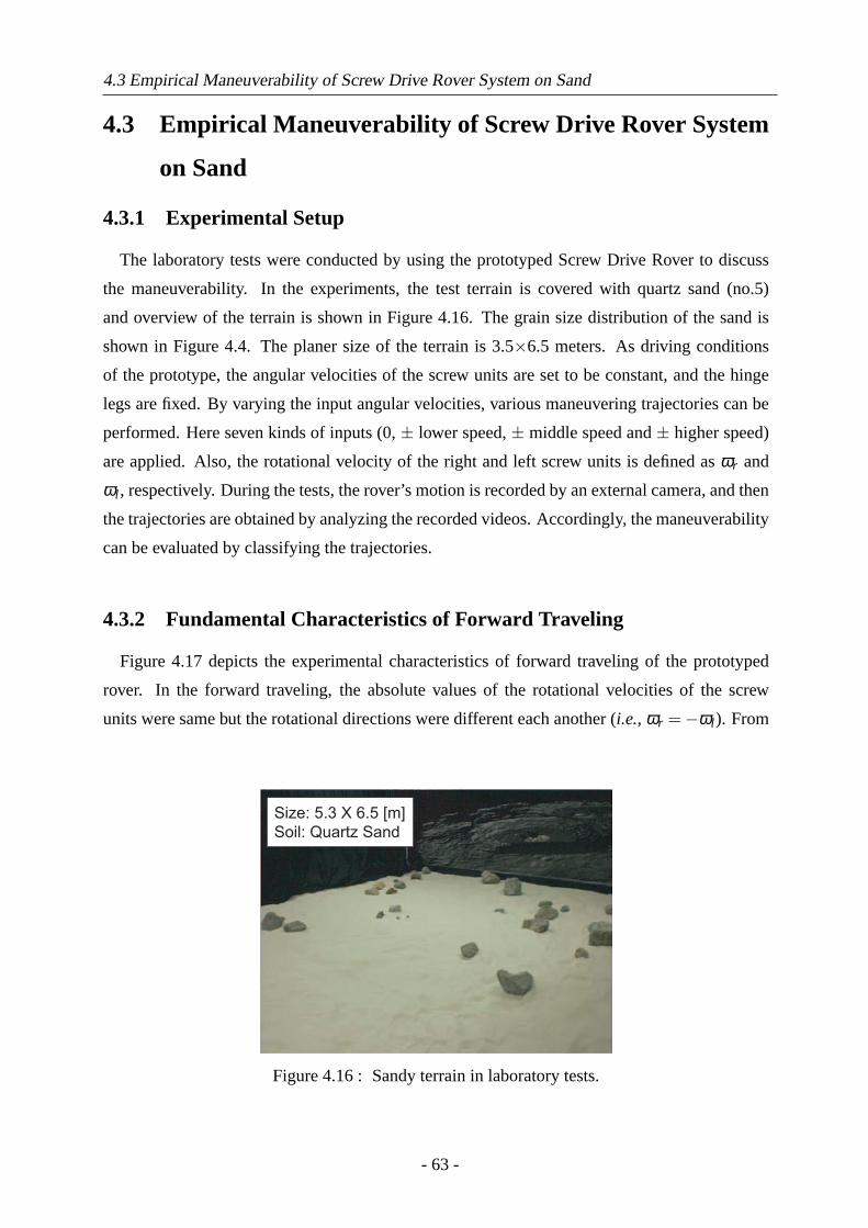
4.3 Empirical Maneuverability of Screw Drive Rover System on Sand
4.3 Empirical Maneuverability of Screw Drive Rover System
on Sand
4.3.1 Experimental Setup
The laboratory tests were conducted by using the prototyped Screw Drive Rover to discuss
the maneuverability. In the experiments, the test terrain is covered with quartz sand (no.5)
and overview of the terrain is shown in Figure 4.16. The grain size distribution of the sand is
shown in Figure 4.4. The planer size of the terrain is 3.5×6.5 meters. As driving conditions
of the prototype, the angular velocities of the screw units are set to be constant, and the hinge
legs are fixed. By varying the input angular velocities, various maneuvering trajectories can be
performed. Here seven kinds of inputs (0,± lower speed,± middle speed and± higher speed)
are applied. Also, the rotational velocity of the right and left screw units is defined asωr and
ωl , respectively. During the tests, the rover’s motion is recorded by an external camera, and then
the trajectories are obtained by analyzing the recorded videos. Accordingly, the maneuverability
can be evaluated by classifying the trajectories.
4.3.2 Fundamental Characteristics of Forward Traveling
Figure 4.17 depicts the experimental characteristics of forward traveling of the prototyped
rover. In the forward traveling, the absolute values of the rotational velocities of the screw
units were same but the rotational directions were different each another (i.e., ωr =−ωl ). From
Size: 5.3 X 6.5 [m]
Soil: Quartz Sand
Figure 4.16 : Sandy terrain in laboratory tests.
- 63 -
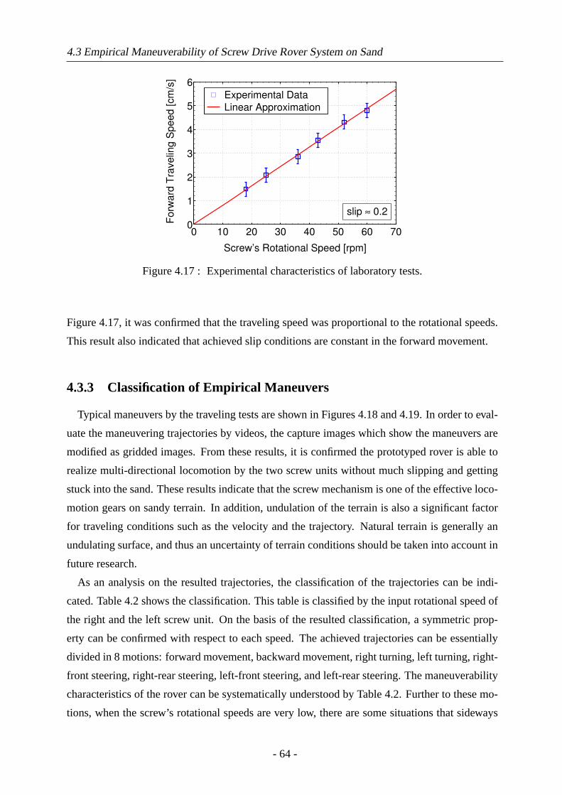
4.3 Empirical Maneuverability of Screw Drive Rover System on Sand
0 10 20 30 40 50 60 700
1
2
3
4
5
6
Screw’s Rotational Speed [rpm]
Fo
rwa
rd T
rave
lin
g S
pe
ed
[cm
/s]
Experimental Data
Linear Approximation
slip ≈ 0.2
Figure 4.17 : Experimental characteristics of laboratory tests.
Figure 4.17, it was confirmed that the traveling speed was proportional to the rotational speeds.
This result also indicated that achieved slip conditions are constant in the forward movement.
4.3.3 Classification of Empirical Maneuvers
Typical maneuvers by the traveling tests are shown in Figures 4.18 and 4.19. In order to eval-
uate the maneuvering trajectories by videos, the capture images which show the maneuvers are
modified as gridded images. From these results, it is confirmed the prototyped rover is able to
realize multi-directional locomotion by the two screw units without much slipping and getting
stuck into the sand. These results indicate that the screw mechanism is one of the effective loco-
motion gears on sandy terrain. In addition, undulation of the terrain is also a significant factor
for traveling conditions such as the velocity and the trajectory. Natural terrain is generally an
undulating surface, and thus an uncertainty of terrain conditions should be taken into account in
future research.
As an analysis on the resulted trajectories, the classification of the trajectories can be indi-
cated. Table 4.2 shows the classification. This table is classified by the input rotational speed of
the right and the left screw unit. On the basis of the resulted classification, a symmetric prop-
erty can be confirmed with respect to each speed. The achieved trajectories can be essentially
divided in 8 motions: forward movement, backward movement, right turning, left turning, right-
front steering, right-rear steering, left-front steering, and left-rear steering. The maneuverability
characteristics of the rover can be systematically understood by Table 4.2. Further to these mo-
tions, when the screw’s rotational speeds are very low, there are some situations that sideways
- 64 -
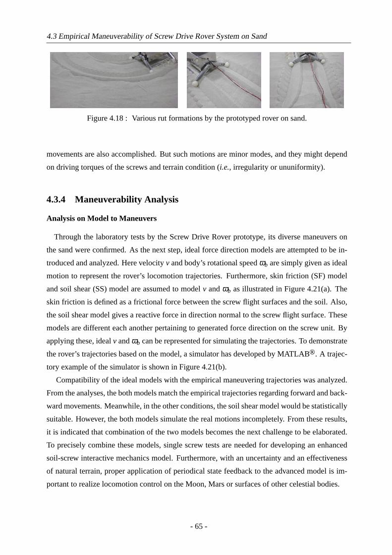
4.3 Empirical Maneuverability of Screw Drive Rover System on Sand
Figure 4.18 : Various rut formations by the prototyped rover on sand.
movements are also accomplished. But such motions are minor modes, and they might depend
on driving torques of the screws and terrain condition (i.e., irregularity or ununiformity).
4.3.4 Maneuverability Analysis
Analysis on Model to Maneuvers
Through the laboratory tests by the Screw Drive Rover prototype, its diverse maneuvers on
the sand were confirmed. As the next step, ideal force direction models are attempted to be in-
troduced and analyzed. Here velocityv and body’s rotational speedωb are simply given as ideal
motion to represent the rover’s locomotion trajectories. Furthermore, skin friction (SF) model
and soil shear (SS) model are assumed to modelv andωb as illustrated in Figure 4.21(a). The
skin friction is defined as a frictional force between the screw flight surfaces and the soil. Also,
the soil shear model gives a reactive force in direction normal to the screw flight surface. These
models are different each another pertaining to generated force direction on the screw unit. By
applying these, idealv andωb can be represented for simulating the trajectories. To demonstrate
the rover’s trajectories based on the model, a simulator has developed by MATLABr. A trajec-
tory example of the simulator is shown in Figure 4.21(b).
Compatibility of the ideal models with the empirical maneuvering trajectories was analyzed.
From the analyses, the both models match the empirical trajectories regarding forward and back-
ward movements. Meanwhile, in the other conditions, the soil shear model would be statistically
suitable. However, the both models simulate the real motions incompletely. From these results,
it is indicated that combination of the two models becomes the next challenge to be elaborated.
To precisely combine these models, single screw tests are needed for developing an enhanced
soil-screw interactive mechanics model. Furthermore, with an uncertainty and an effectiveness
of natural terrain, proper application of periodical state feedback to the advanced model is im-
portant to realize locomotion control on the Moon, Mars or surfaces of other celestial bodies.
- 65 -
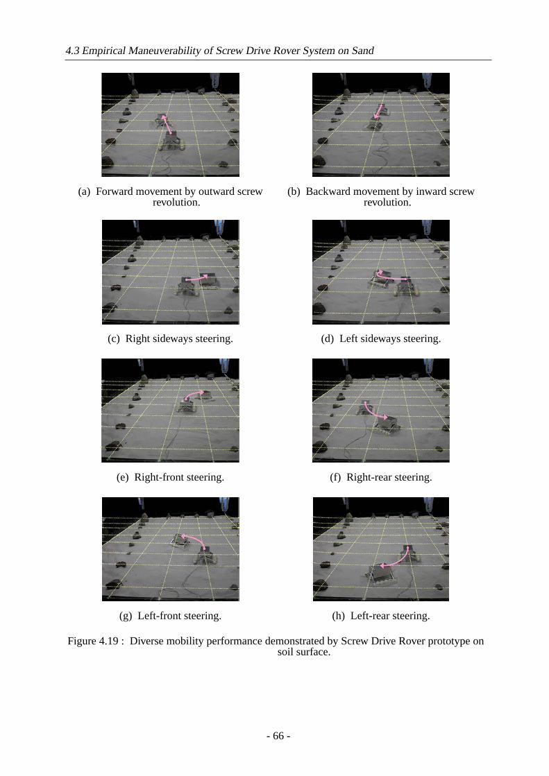
4.3 Empirical Maneuverability of Screw Drive Rover System on Sand
(a) Forward movement by outward screwrevolution.
(b) Backward movement by inward screwrevolution.
(c) Right sideways steering. (d) Left sideways steering.
(e) Right-front steering. (f) Right-rear steering.
(g) Left-front steering. (h) Left-rear steering.
Figure 4.19 : Diverse mobility performance demonstrated by Screw Drive Rover prototype onsoil surface.
- 66 -
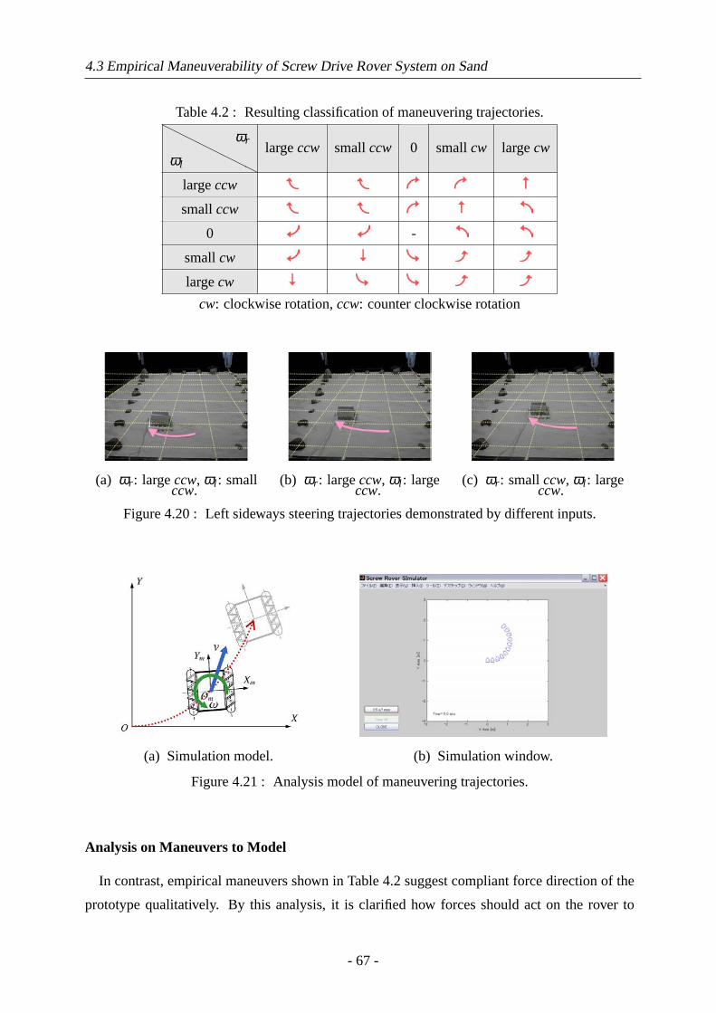
4.3 Empirical Maneuverability of Screw Drive Rover System on Sand
Table 4.2 : Resulting classification of maneuvering trajectories.HHHHHHHH
ωl
ωrlargeccw smallccw 0 smallcw largecw
largeccw
smallccw
0 -
smallcw
largecw
cw: clockwise rotation,ccw: counter clockwise rotation
(a) ωr : largeccw, ωl : smallccw.
(b) ωr : largeccw, ωl : largeccw.
(c) ωr : smallccw, ωl : largeccw.
Figure 4.20 : Left sideways steering trajectories demonstrated by different inputs.
(a) Simulation model. (b) Simulation window.
Figure 4.21 : Analysis model of maneuvering trajectories.
Analysis on Maneuvers to Model
In contrast, empirical maneuvers shown in Table 4.2 suggest compliant force direction of the
prototype qualitatively. By this analysis, it is clarified how forces should act on the rover to
- 67 -
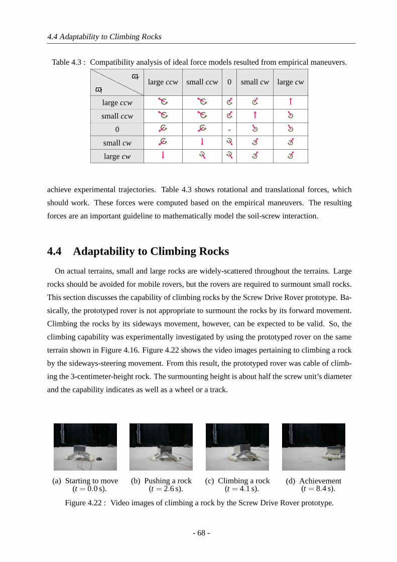
4.4 Adaptability to Climbing Rocks
Table 4.3 : Compatibility analysis of ideal force models resulted from empirical maneuvers.HHHHHHHH
ωl
ωrlargeccw smallccw 0 smallcw largecw
largeccw
smallccw
0 -
smallcw
largecw
achieve experimental trajectories. Table 4.3 shows rotational and translational forces, which
should work. These forces were computed based on the empirical maneuvers. The resulting
forces are an important guideline to mathematically model the soil-screw interaction.
4.4 Adaptability to Climbing Rocks
On actual terrains, small and large rocks are widely-scattered throughout the terrains. Large
rocks should be avoided for mobile rovers, but the rovers are required to surmount small rocks.
This section discusses the capability of climbing rocks by the Screw Drive Rover prototype. Ba-
sically, the prototyped rover is not appropriate to surmount the rocks by its forward movement.
Climbing the rocks by its sideways movement, however, can be expected to be valid. So, the
climbing capability was experimentally investigated by using the prototyped rover on the same
terrain shown in Figure 4.16. Figure 4.22 shows the video images pertaining to climbing a rock
by the sideways-steering movement. From this result, the prototyped rover was cable of climb-
ing the 3-centimeter-height rock. The surmounting height is about half the screw unit’s diameter
and the capability indicates as well as a wheel or a track.
(a) Starting to move(t = 0.0s).
(b) Pushing a rock(t = 2.6s).
(c) Climbing a rock(t = 4.1s).
(d) Achievement(t = 8.4s).
Figure 4.22 : Video images of climbing a rock by the Screw Drive Rover prototype.
- 68 -
4.5 Summary
4.5 Summary
This chapter presents the surface locomotion technique by the Archimedean screw units. Such
locomotion method is on especially expected to exert better performance on the soft terrain be-
cause of its robustness to getting stuck. Meanwhile, academic researches on the surface loco-
motion by the screw units have been rarely conducted. So, at first, this dissertation attempted
to accumulate engineering knowledge about the surface locomotion by the screw units. Specifi-
cally, the following two terms were experimentally studied:
Analysis on Empirical Trafficability
The fundamental trafficability of the single screw unit was investigated. To examine the
trafficability, the laboratory tests were carried out as well as the maneuverability analysis.
The experimental results showed the significant tendency that the drawbar pull increases
with an increase of the slip, regardless of the load and the rotational velocity. Moreover,
it was confirmed that the load and the rotational velocity did not affect the characteris-
tics of the drawbar pull and the slip. On the contrary, the slip angle had much effect on
the characteristics. This result leads to understanding of the propulsive force direction,
and then enables synthetic discussions with the empirical maneuvers. Furthermore, com-
parative analyses were conducted by the experiments and the simulations. According to
these, it was confirmed that the simulation plots by using the proposed model can meet
the experimental results.
Analysis on Empirical Maneuverability
In this research, the Screw Drive Rover employing the dual screw units was proposed for
a practical application system. As for mobility performance of the proposed system, its
empirical maneuverability was elaborated through laboratory tests. From this elaboration,
the maneuvering trajectories demonstrated by the system were analyzed and discussed.
In addition to this, the empirical maneuvers enable to understand the propulsive force
direction in each maneuver.
- 69 -

4.5 Summary
- 70 -
Chapter 5. Modeling and Analysis of
Screw Subsurface
Locomotion
5.1 Expectation for Lunar Subsurface Exploration
Recently, Lunar exploration has received a lot of renewed attention. A lot of scientific ques-
tions have remained unanswered concerning the Moon’s origin, its evolution or chemical com-
position [6–8]. Unmanned robotic exploration of the lunar subsurface is getting more critical in
the process of answering these questions. This will require developing more capable subsurface
robotic exploration devices [174]. But, the conventionalin situ approach of the lunar material
can only provide localized measurements which cannot be extended to characterize large areas
around the chosen sampling site. Implanting scientific instruments on the actual sampling site
could potentially provide more information on a larger scale, which could ultimately help deter-
mining the global internal structure of the Moon, especially its core. The long term measurement
on the Moon is arduous since ultra-cold temperature seriously limits power generation from pho-
tovoltaic cells at night. In the case of the Apollo lunar landing missions by NASA, a passive
seismic network by 4 stations (at the Apollo 12, 14, 15 and 16 landing sites) was constructed to
investigate lunar seismicity [3]. Figure 5.1 shows the Apollo 16 seismometer deployed on the
Moon. By measuring lunar seismic events, The Passive Seismic Experiment (PES) produced the
partial knowledge of the lunar interior structure, the distribution of the lunar seismic sources and
the attenuation of the seismic waves. The seismometers were in a thermal shroud with a 20 layer
multi-layer-insulation (MLI) as seen in Figure 5.1. In addition to this, the seismometers used
thermal control instruments such as radioisotope heaters to survive lunar night. However, iso-
topes used in the radioisotope heaters have strong disadvantages (high toxicity, short half life and
restricted availability), so that other methods without the radioisotope heaters are to be consid-
ered as alternatives [9]. So this dissertation focuses on a robotic system for burying a scientific
instrument (such as a long-term seismometer) in the subsurface, effectively and continuously
stabilizing its temperature environment by the thermal insulation of the lunar soil surrounding
- 71 -
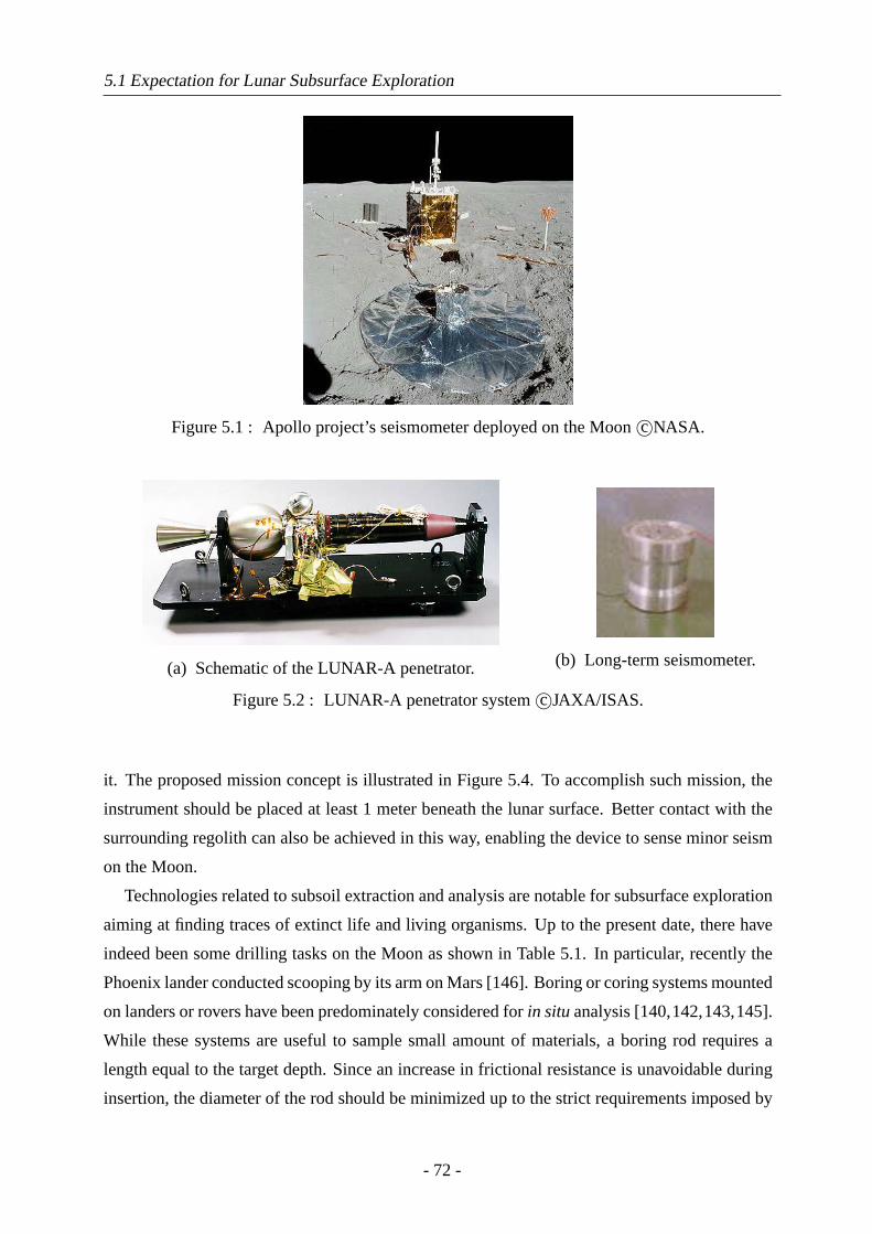
5.1 Expectation for Lunar Subsurface Exploration
Figure 5.1 : Apollo project’s seismometer deployed on the Moonc©NASA.
(a) Schematic of the LUNAR-A penetrator. (b) Long-term seismometer.
Figure 5.2 : LUNAR-A penetrator systemc©JAXA/ISAS.
it. The proposed mission concept is illustrated in Figure 5.4. To accomplish such mission, the
instrument should be placed at least 1 meter beneath the lunar surface. Better contact with the
surrounding regolith can also be achieved in this way, enabling the device to sense minor seism
on the Moon.
Technologies related to subsoil extraction and analysis are notable for subsurface exploration
aiming at finding traces of extinct life and living organisms. Up to the present date, there have
indeed been some drilling tasks on the Moon as shown in Table 5.1. In particular, recently the
Phoenix lander conducted scooping by its arm on Mars [146]. Boring or coring systems mounted
on landers or rovers have been predominately considered forin situanalysis [140,142,143,145].
While these systems are useful to sample small amount of materials, a boring rod requires a
length equal to the target depth. Since an increase in frictional resistance is unavoidable during
insertion, the diameter of the rod should be minimized up to the strict requirements imposed by
- 72 -
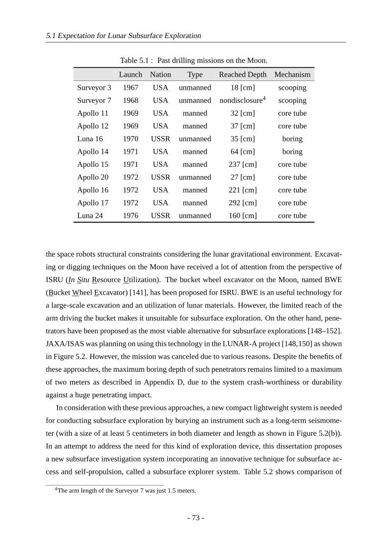
5.1 Expectation for Lunar Subsurface Exploration
Table 5.1 : Past drilling missions on the Moon.
Launch Nation Type Reached Depth Mechanism
Surveyor 3 1967 USA unmanned 18 [cm] scooping
Surveyor 7 1968 USA unmanned nondisclosure4 scooping
Apollo 11 1969 USA manned 32 [cm] core tube
Apollo 12 1969 USA manned 37 [cm] core tube
Luna 16 1970 USSR unmanned 35 [cm] boring
Apollo 14 1971 USA manned 64 [cm] boring
Apollo 15 1971 USA manned 237 [cm] core tube
Apollo 20 1972 USSR unmanned 27 [cm] core tube
Apollo 16 1972 USA manned 221 [cm] core tube
Apollo 17 1972 USA manned 292 [cm] core tube
Luna 24 1976 USSR unmanned 160 [cm] core tube
the space robots structural constraints considering the lunar gravitational environment. Excavat-
ing or digging techniques on the Moon have received a lot of attention from the perspective of
ISRU (In Situ Resource Utilization). The bucket wheel excavator on the Moon, named BWE
(Bucket Wheel Excavator) [141], has been proposed for ISRU. BWE is an useful technology for
a large-scale excavation and an utilization of lunar materials. However, the limited reach of the
arm driving the bucket makes it unsuitable for subsurface exploration. On the other hand, pene-
trators have been proposed as the most viable alternative for subsurface explorations [148–152].
JAXA/ISAS was planning on using this technology in the LUNAR-A project [148,150] as shown
in Figure 5.2. However, the mission was canceled due to various reasons. Despite the benefits of
these approaches, the maximum boring depth of such penetrators remains limited to a maximum
of two meters as described in Appendix D, due to the system crash-worthiness or durability
against a huge penetrating impact.
In consideration with these previous approaches, a new compact lightweight system is needed
for conducting subsurface exploration by burying an instrument such as a long-term seismome-
ter (with a size of at least 5 centimeters in both diameter and length as shown in Figure 5.2(b)).
In an attempt to address the need for this kind of exploration device, this dissertation proposes
a new subsurface investigation system incorporating an innovative technique for subsurface ac-
cess and self-propulsion, called a subsurface explorer system. Table 5.2 shows comparison of
4The arm length of the Surveyor 7 was just 1.5 meters.
- 73 -
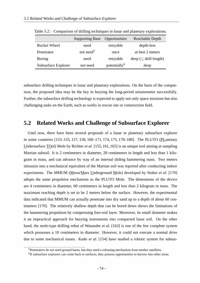
5.2 Related Works and Challenge of Subsurface Explorer
Table 5.2 : Comparison of drilling techniques in lunar and planetary explorations.
Supporting Base Opportunities Reachable Depth
Bucket Wheel need retryable depth-less
Penetrator not need5 once at best 2 meters
Boring need retryable deep (≤ drill length)
Subsurface Explorer not need potentially6 deep
subsurface drilling techniques in lunar and planetary explorations. On the basis of the compar-
ison, the proposed idea may be the key in burying the long-period seismometer successfully.
Further, the subsurface drilling technology is expected to apply not only space missions but also
challenging tasks on the Earth, such as works in rescue site or construction field.
5.2 Related Works and Challenge of Subsurface Explorer
Until now, there have been several proposals of a lunar or planetary subsurface explorer
in some countries [153–155, 157, 158, 160–171, 174, 175, 178–180]. The PLUTO (PLanetary
Undersurface TOol) Mole by Richteret al. [155,161,165] is an unique tool aiming at sampling
Martian subsoil. It is 2 centimeters in diameter, 28 centimeters in length and less than 1 kilo-
gram in mass, and can advance by way of an internal sliding hammering mass. Two meters
intrusion into a mechanical equivalent of the Martian soil was reported after conducting indoor
experiments. The MMUM (Moon/Mars Underground Mole) developed by Stokeret al. [170]
adopts the same propulsive mechanism as the PLUTO Mole. The dimensions of the device
are 4 centimeters in diameter, 60 centimeters in length and less than 2 kilogram in mass. The
maximum reaching depth is set to be 2 meters below the surface. However, the experimental
data indicated that MMUM can actually penetrate into dry sand up to a depth of about 60 cen-
timeters [170]. The relatively shallow depth that can be bored down shows the limitations of
the hammering propulsion by compressing fore-soil layer. Moreover, its small diameter makes
it an impractical approach for burying instruments into compacted lunar soil. On the other
hand, the mole-type drilling robot of Watanabeet al. [163] is one of the few complete system
which possesses a 10 centimeters in diameter. However, it could not execute a normal drive
due to some mechanical issues. Kudoet al. [154] have studied a robotic system for subsur-
5Penetrators do not need ground bases, but they need a releasing mechanism from mother satellites.6If subsurface explorers can come back to surfaces, they possess opportunities to burrow into other areas.
- 74 -
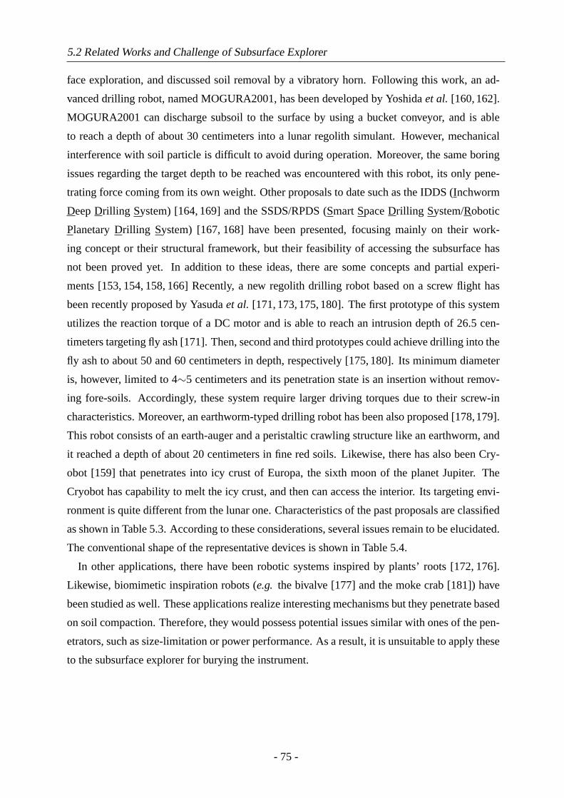
5.2 Related Works and Challenge of Subsurface Explorer
face exploration, and discussed soil removal by a vibratory horn. Following this work, an ad-
vanced drilling robot, named MOGURA2001, has been developed by Yoshidaet al. [160,162].
MOGURA2001 can discharge subsoil to the surface by using a bucket conveyor, and is able
to reach a depth of about 30 centimeters into a lunar regolith simulant. However, mechanical
interference with soil particle is difficult to avoid during operation. Moreover, the same boring
issues regarding the target depth to be reached was encountered with this robot, its only pene-
trating force coming from its own weight. Other proposals to date such as the IDDS (Inchworm
Deep Drilling System) [164, 169] and the SSDS/RPDS (Smart Space Drilling System/Robotic
Planetary Drilling System) [167, 168] have been presented, focusing mainly on their work-
ing concept or their structural framework, but their feasibility of accessing the subsurface has
not been proved yet. In addition to these ideas, there are some concepts and partial experi-
ments [153, 154, 158, 166] Recently, a new regolith drilling robot based on a screw flight has
been recently proposed by Yasudaet al. [171, 173, 175, 180]. The first prototype of this system
utilizes the reaction torque of a DC motor and is able to reach an intrusion depth of 26.5 cen-
timeters targeting fly ash [171]. Then, second and third prototypes could achieve drilling into the
fly ash to about 50 and 60 centimeters in depth, respectively [175, 180]. Its minimum diameter
is, however, limited to 4∼5 centimeters and its penetration state is an insertion without remov-
ing fore-soils. Accordingly, these system require larger driving torques due to their screw-in
characteristics. Moreover, an earthworm-typed drilling robot has been also proposed [178,179].
This robot consists of an earth-auger and a peristaltic crawling structure like an earthworm, and
it reached a depth of about 20 centimeters in fine red soils. Likewise, there has also been Cry-
obot [159] that penetrates into icy crust of Europa, the sixth moon of the planet Jupiter. The
Cryobot has capability to melt the icy crust, and then can access the interior. Its targeting envi-
ronment is quite different from the lunar one. Characteristics of the past proposals are classified
as shown in Table 5.3. According to these considerations, several issues remain to be elucidated.
The conventional shape of the representative devices is shown in Table 5.4.
In other applications, there have been robotic systems inspired by plants’ roots [172, 176].
Likewise, biomimetic inspiration robots (e.g. the bivalve [177] and the moke crab [181]) have
been studied as well. These applications realize interesting mechanisms but they penetrate based
on soil compaction. Therefore, they would possess potential issues similar with ones of the pen-
etrators, such as size-limitation or power performance. As a result, it is unsuitable to apply these
to the subsurface explorer for burying the instrument.
- 75 -
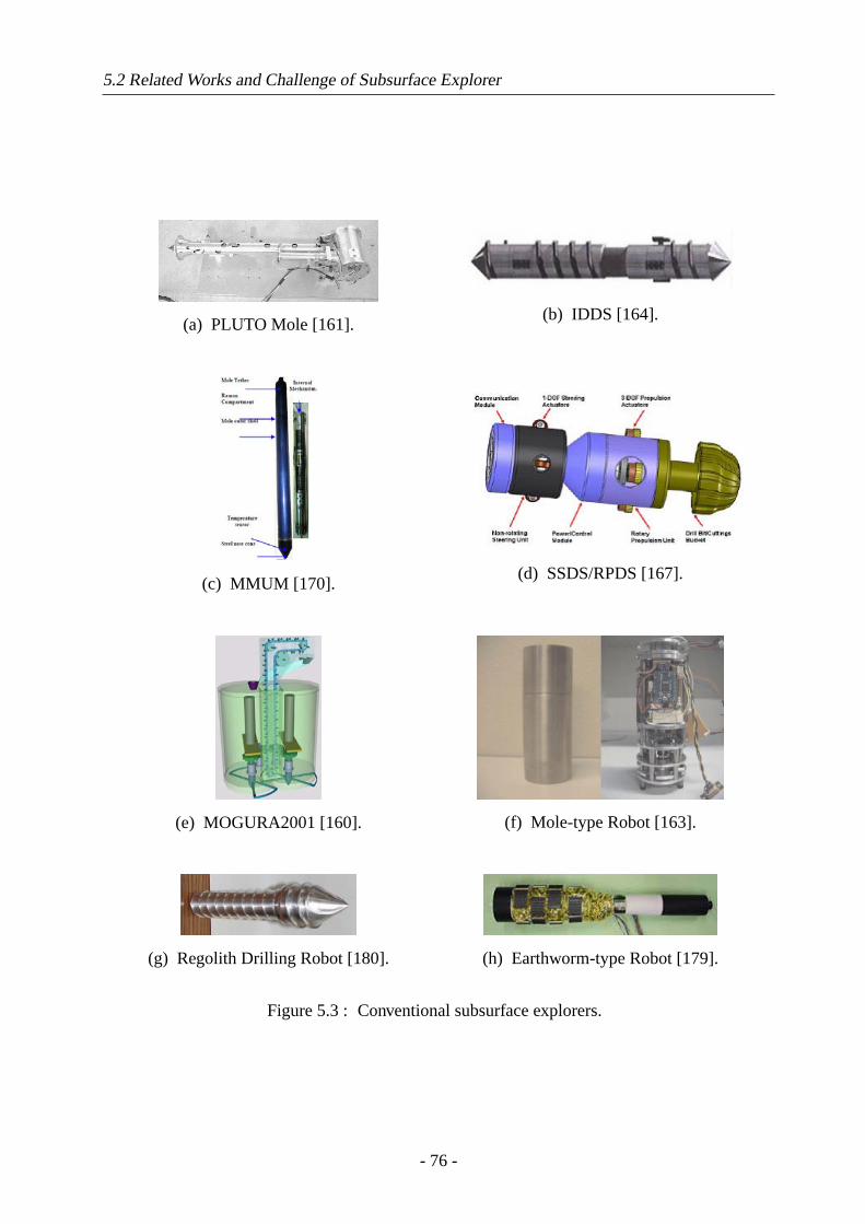
5.2 Related Works and Challenge of Subsurface Explorer
(a) PLUTO Mole [161].(b) IDDS [164].
(c) MMUM [170].(d) SSDS/RPDS [167].
(e) MOGURA2001 [160]. (f) Mole-type Robot [163].
(g) Regolith Drilling Robot [180]. (h) Earthworm-type Robot [179].
Figure 5.3 : Conventional subsurface explorers.
- 76 -
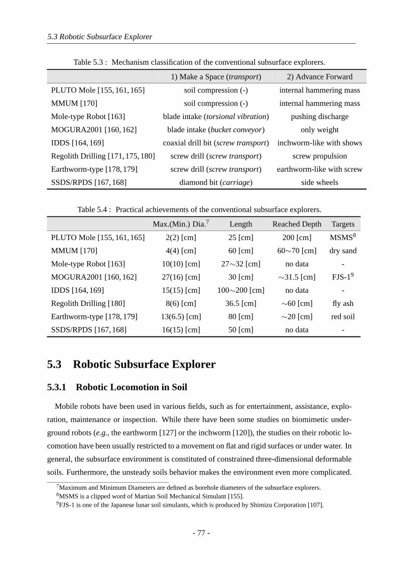
5.3 Robotic Subsurface Explorer
Table 5.3 : Mechanism classification of the conventional subsurface explorers.
1) Make a Space (transport) 2) Advance Forward
PLUTO Mole [155,161,165] soil compression (-) internal hammering mass
MMUM [170] soil compression (-) internal hammering mass
Mole-type Robot [163] blade intake (torsional vibration) pushing discharge
MOGURA2001 [160,162] blade intake (bucket conveyor) only weight
IDDS [164,169] coaxial drill bit (screw transport) inchworm-like with shows
Regolith Drilling [171,175,180] screw drill (screw transport) screw propulsion
Earthworm-type [178,179] screw drill (screw transport) earthworm-like with screw
SSDS/RPDS [167,168] diamond bit (carriage) side wheels
Table 5.4 : Practical achievements of the conventional subsurface explorers.
Max.(Min.) Dia.7 Length Reached Depth Targets
PLUTO Mole [155,161,165] 2(2) [cm] 25 [cm] 200 [cm] MSMS8
MMUM [170] 4(4) [cm] 60 [cm] 60∼70 [cm] dry sand
Mole-type Robot [163] 10(10) [cm] 27∼32 [cm] no data -
MOGURA2001 [160,162] 27(16) [cm] 30 [cm] ∼31.5 [cm] FJS-19
IDDS [164,169] 15(15) [cm] 100∼200 [cm] no data -
Regolith Drilling [180] 8(6) [cm] 36.5 [cm] ∼60 [cm] fly ash
Earthworm-type [178,179] 13(6.5) [cm] 80 [cm] ∼20 [cm] red soil
SSDS/RPDS [167,168] 16(15) [cm] 50 [cm] no data -
5.3 Robotic Subsurface Explorer
5.3.1 Robotic Locomotion in Soil
Mobile robots have been used in various fields, such as for entertainment, assistance, explo-
ration, maintenance or inspection. While there have been some studies on biomimetic under-
ground robots (e.g., the earthworm [127] or the inchworm [120]), the studies on their robotic lo-
comotion have been usually restricted to a movement on flat and rigid surfaces or under water. In
general, the subsurface environment is constituted of constrained three-dimensional deformable
soils. Furthermore, the unsteady soils behavior makes the environment even more complicated.
7Maximum and Minimum Diameters are defined as borehole diameters of the subsurface explorers.8MSMS is a clipped word of Martian Soil Mechanical Simulant [155].9FJS-1 is one of the Japanese lunar soil simulants, which is produced by Shimizu Corporation [107].
- 77 -
5.3 Robotic Subsurface Explorer
Despite this added complexity, robotic subsurface explorers have some unique merits for future
lunar mission:
• Reachable depth is not mechanically limited by the robot length.
• Large bases on the surface is not required for penetration.
• System can be compact size, lightweight and low power.
• Expansion to multiple applications in space developments can be expected;e.g., burying
scientific instruments,in situ analysis, artificial seisms or construction tasks.
5.3.2 Synopsis of Robotic Subsurface Explorer System
In particular, lunar robotic applications needs to accommodate harsh conditions such as ultra-
high vacuum, low gravity, wide temperature variation, and requires being able to operate on or
within the fine regolith layer. The schematic of the proposed mission sequences are illustrated
in Figure 5.4. The following assumptions are set forth regarding the lunar robotic subsurface
exploration system:
• A Micro Rover shall carry the subsurface explorer to the target area.
• The Subsurface Explorer shall be tethered to the Micro Rover for power supply.
• The Subsurface Explorer shall be about 0.1 meters in diameter since the long-term seis-
mometer’s diameter shall be about 0.05 meters.
• Target depth shall be set to a few meters beneath the lunar surface.
• Target soil-layer is assumed to be lunar regolith, which is high frictional and high cohesive
soil, and has large relative density under shallow zone [1–3].
• The lunar gravitational field is assumed to be almost constant for the robot system [4].
5.3.3 Subsurface Locomotion Principle
Systematic Synopsis
Realization of a locomotion mechanism in the subsurface environment is a challenging task,
and is quite difficult to model mathematically. In light of the few studies concerning subsurface
- 78 -
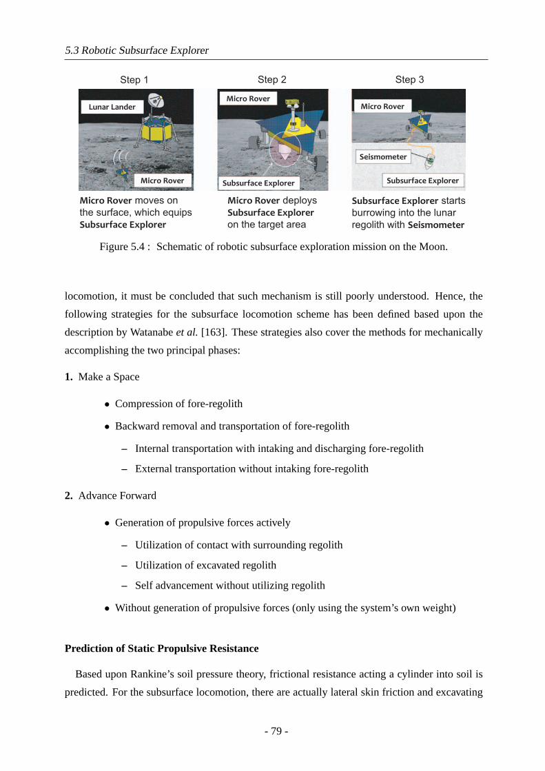
5.3 Robotic Subsurface Explorer
Lunar Lander
Micro Rover
Micro Rover
Subsurface Explorer Subsurface Explorer
Step 3Step 2Step 1
Seismometer
Micro Rover
Micro Rover moves on
the surface, which equips
Subsurface Explorer
Micro Rover deploys
Subsurface Explorer
on the target area
Subsurface Explorer starts
burrowing into the lunar
regolith with Seismometer
Figure 5.4 : Schematic of robotic subsurface exploration mission on the Moon.
locomotion, it must be concluded that such mechanism is still poorly understood. Hence, the
following strategies for the subsurface locomotion scheme has been defined based upon the
description by Watanabeet al. [163]. These strategies also cover the methods for mechanically
accomplishing the two principal phases:
1. Make a Space
• Compression of fore-regolith
• Backward removal and transportation of fore-regolith
– Internal transportation with intaking and discharging fore-regolith
– External transportation without intaking fore-regolith
2. Advance Forward
• Generation of propulsive forces actively
– Utilization of contact with surrounding regolith
– Utilization of excavated regolith
– Self advancement without utilizing regolith
• Without generation of propulsive forces (only using the system’s own weight)
Prediction of Static Propulsive Resistance
Based upon Rankine’s soil pressure theory, frictional resistance acting a cylinder into soil is
predicted. For the subsurface locomotion, there are actually lateral skin friction and excavating
- 79 -
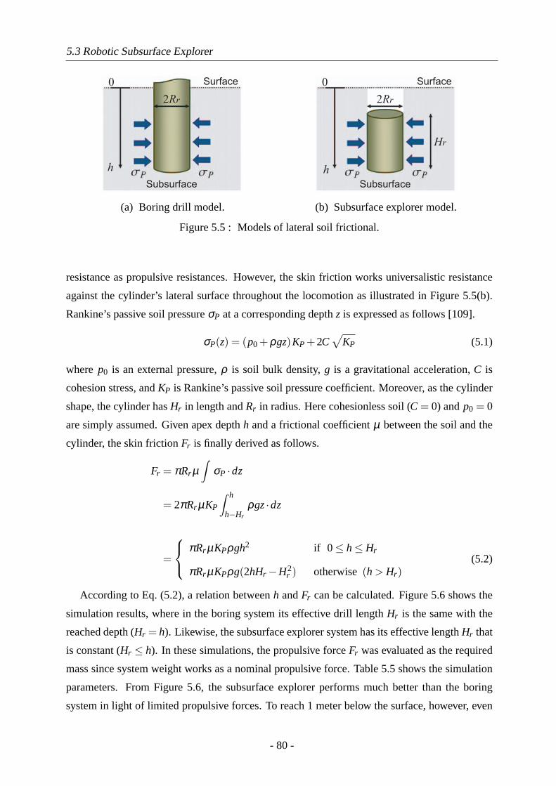
5.3 Robotic Subsurface Explorer
Surface
h
2Rr
Subsurface
0
(a) Boring drill model.
Surface
Hr
2Rr
Subsurface
0
h
(b) Subsurface explorer model.
Figure 5.5 : Models of lateral soil frictional.
resistance as propulsive resistances. However, the skin friction works universalistic resistance
against the cylinder’s lateral surface throughout the locomotion as illustrated in Figure 5.5(b).
Rankine’s passive soil pressureσP at a corresponding depthz is expressed as follows [109].
σP(z) = (p0 +ρgz)KP +2C√
KP (5.1)
wherep0 is an external pressure,ρ is soil bulk density,g is a gravitational acceleration,C is
cohesion stress, andKP is Rankine’s passive soil pressure coefficient. Moreover, as the cylinder
shape, the cylinder hasHr in length andRr in radius. Here cohesionless soil (C = 0) andp0 = 0
are simply assumed. Given apex depthh and a frictional coefficientµ between the soil and the
cylinder, the skin frictionFr is finally derived as follows.
Fr = πRr µ∫
σP ·dz
= 2πRr µKP
∫ h
h−Hr
ρgz·dz
=
πRr µKPρgh2 if 0≤ h≤ Hr
πRr µKPρg(2hHr −H2r ) otherwise(h > Hr)
(5.2)
According to Eq. (5.2), a relation betweenh andFr can be calculated. Figure 5.6 shows the
simulation results, where in the boring system its effective drill lengthHr is the same with the
reached depth (Hr = h). Likewise, the subsurface explorer system has its effective lengthHr that
is constant (Hr ≤ h). In these simulations, the propulsive forceFr was evaluated as the required
mass since system weight works as a nominal propulsive force. Table 5.5 shows the simulation
parameters. From Figure 5.6, the subsurface explorer performs much better than the boring
system in light of limited propulsive forces. To reach 1 meter below the surface, however, even
- 80 -
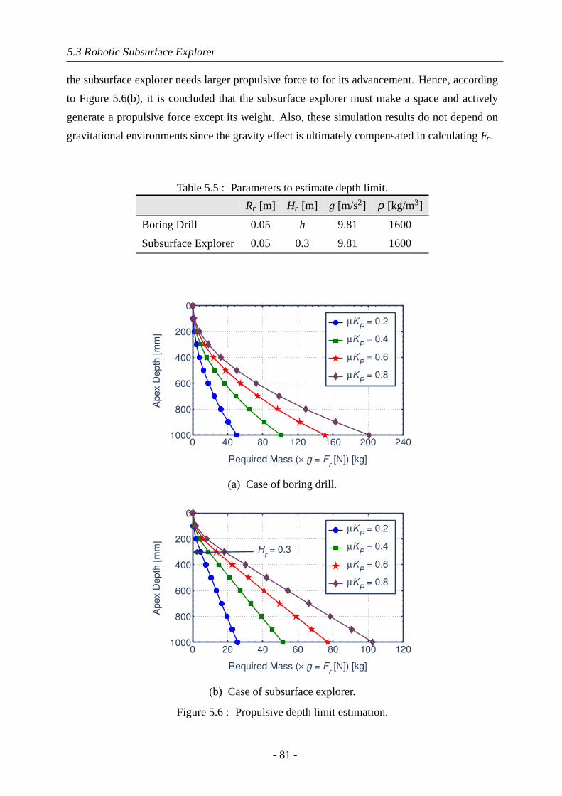
5.3 Robotic Subsurface Explorer
the subsurface explorer needs larger propulsive force to for its advancement. Hence, according
to Figure 5.6(b), it is concluded that the subsurface explorer must make a space and actively
generate a propulsive force except its weight. Also, these simulation results do not depend on
gravitational environments since the gravity effect is ultimately compensated in calculatingFr .
Table 5.5 : Parameters to estimate depth limit.
Rr [m] Hr [m] g [m/s2] ρ [kg/m3]
Boring Drill 0.05 h 9.81 1600
Subsurface Explorer 0.05 0.3 9.81 1600
0 40 80 120 160 200 240
0
200
400
600
800
1000
Required Mass (× g = Fr [N]) [kg]
Apex D
epth
[m
m]
µKP = 0.2
µKP = 0.4
µKP = 0.6
µKP = 0.8
(a) Case of boring drill.
0 20 40 60 80 100 120
0
200
400
600
800
1000
Required Mass (× g = Fr [N]) [kg]
Apex D
epth
[m
m]
µKP = 0.2
µKP = 0.4
µKP = 0.6
µKP = 0.8
Hr = 0.3
(b) Case of subsurface explorer.
Figure 5.6 : Propulsive depth limit estimation.
- 81 -
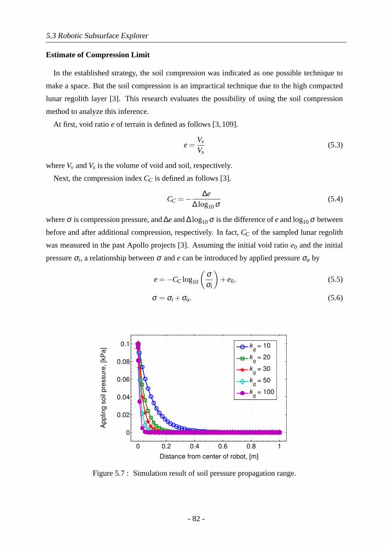
5.3 Robotic Subsurface Explorer
Estimate of Compression Limit
In the established strategy, the soil compression was indicated as one possible technique to
make a space. But the soil compression is an impractical technique due to the high compacted
lunar regolith layer [3]. This research evaluates the possibility of using the soil compression
method to analyze this inference.
At first, void ratioeof terrain is defined as follows [3,109].
e=Vv
Vs(5.3)
whereVv andVs is the volume of void and soil, respectively.
Next, the compression indexCC is defined as follows [3].
CC =− ∆e∆ log10σ
(5.4)
whereσ is compression pressure, and∆eand∆ log10σ is the difference ofeandlog10σ between
before and after additional compression, respectively. In fact,CC of the sampled lunar regolith
was measured in the past Apollo projects [3]. Assuming the initial void ratioe0 and the initial
pressureσi , a relationship betweenσ andecan be introduced by applied pressureσa by
e=−CC log10
(σσi
)+e0, (5.5)
σ = σi +σa. (5.6)
0 0.2 0.4 0.6 0.8 1
0
0.02
0.04
0.06
0.08
0.1
Distance from center of robot, [m]
Appling s
oil p
ressure
, [k
Pa]
kq = 10
kq = 20
kq = 30
kq = 50
kq = 100
Figure 5.7 : Simulation result of soil pressure propagation range.
- 82 -
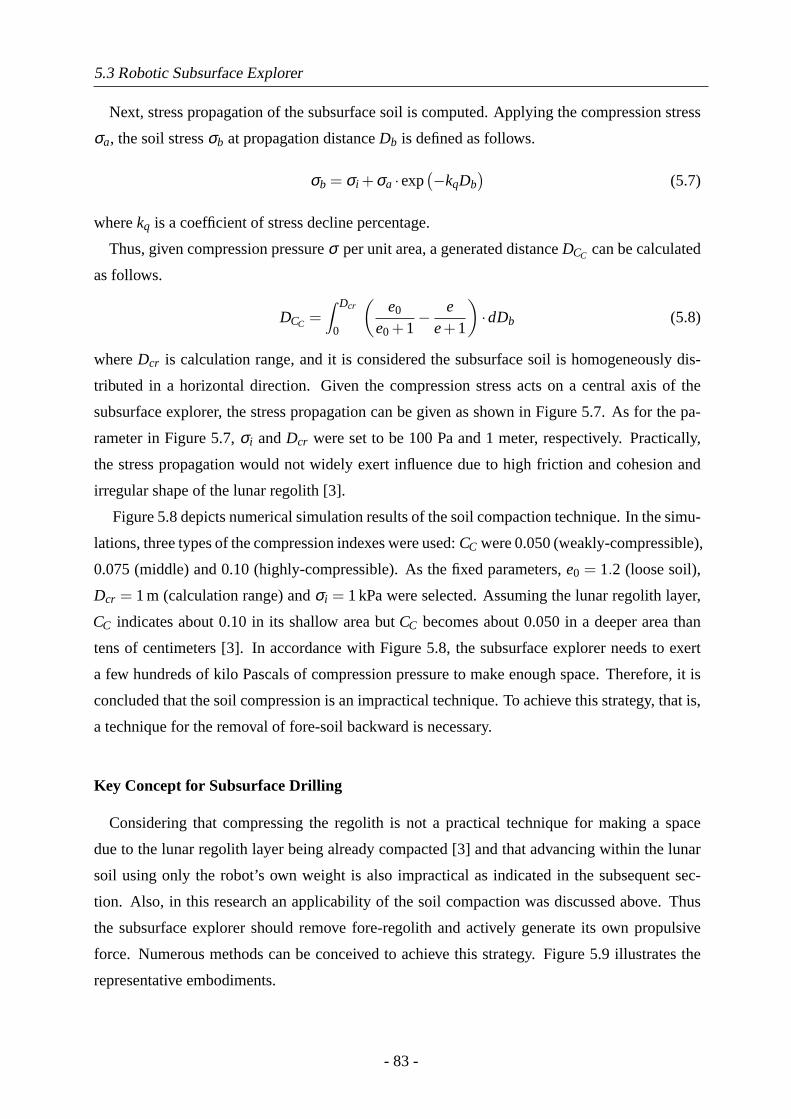
5.3 Robotic Subsurface Explorer
Next, stress propagation of the subsurface soil is computed. Applying the compression stress
σa, the soil stressσb at propagation distanceDb is defined as follows.
σb = σi +σa ·exp(−kqDb
)(5.7)
wherekq is a coefficient of stress decline percentage.
Thus, given compression pressureσ per unit area, a generated distanceDCC can be calculated
as follows.
DCC =∫ Dcr
0
(e0
e0 +1− e
e+1
)·dDb (5.8)
whereDcr is calculation range, and it is considered the subsurface soil is homogeneously dis-
tributed in a horizontal direction. Given the compression stress acts on a central axis of the
subsurface explorer, the stress propagation can be given as shown in Figure 5.7. As for the pa-
rameter in Figure 5.7,σi andDcr were set to be 100 Pa and 1 meter, respectively. Practically,
the stress propagation would not widely exert influence due to high friction and cohesion and
irregular shape of the lunar regolith [3].
Figure 5.8 depicts numerical simulation results of the soil compaction technique. In the simu-
lations, three types of the compression indexes were used:CC were 0.050 (weakly-compressible),
0.075 (middle) and 0.10 (highly-compressible). As the fixed parameters,e0 = 1.2 (loose soil),
Dcr = 1m (calculation range) andσi = 1kPa were selected. Assuming the lunar regolith layer,
CC indicates about 0.10 in its shallow area butCC becomes about 0.050 in a deeper area than
tens of centimeters [3]. In accordance with Figure 5.8, the subsurface explorer needs to exert
a few hundreds of kilo Pascals of compression pressure to make enough space. Therefore, it is
concluded that the soil compression is an impractical technique. To achieve this strategy, that is,
a technique for the removal of fore-soil backward is necessary.
Key Concept for Subsurface Drilling
Considering that compressing the regolith is not a practical technique for making a space
due to the lunar regolith layer being already compacted [3] and that advancing within the lunar
soil using only the robot’s own weight is also impractical as indicated in the subsequent sec-
tion. Also, in this research an applicability of the soil compaction was discussed above. Thus
the subsurface explorer should remove fore-regolith and actively generate its own propulsive
force. Numerous methods can be conceived to achieve this strategy. Figure 5.9 illustrates the
representative embodiments.
- 83 -
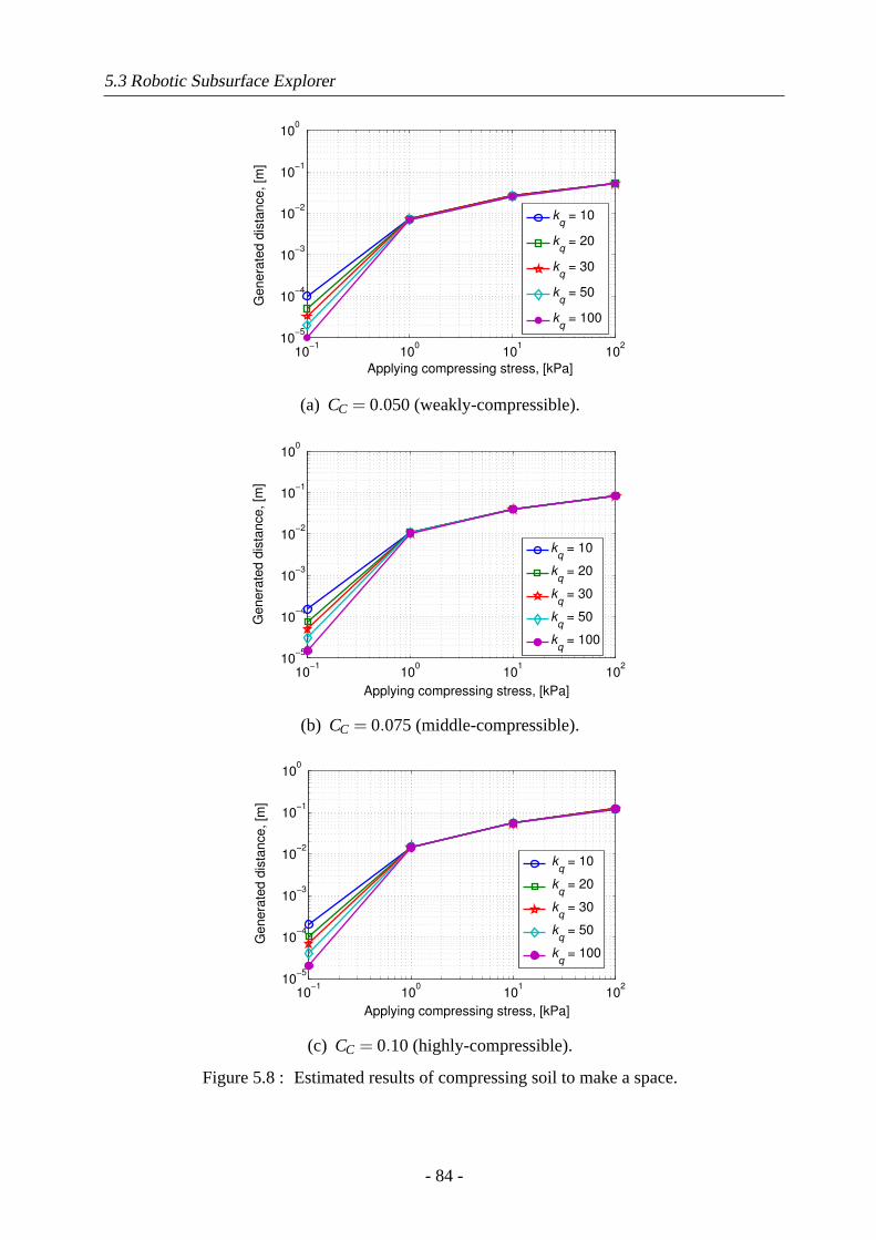
5.3 Robotic Subsurface Explorer
10−1
100
101
102
10−5
10−4
10−3
10−2
10−1
100
Genera
ted d
ista
nce, [m
]
Applying compressing stress, [kPa]
kq = 10
kq = 20
kq = 30
kq = 50
kq = 100
(a) CC = 0.050(weakly-compressible).
10−1
100
101
102
10−5
10−4
10−3
10−2
10−1
100
Genera
ted d
ista
nce, [m
]
Applying compressing stress, [kPa]
kq = 10
kq = 20
kq = 30
kq = 50
kq = 100
(b) CC = 0.075(middle-compressible).
10−1
100
101
102
10−5
10−4
10−3
10−2
10−1
100
Applying compressing stress, [kPa]
Genera
ted d
ista
nce, [m
]
kq = 10
kq = 20
kq = 30
kq = 50
kq = 100
(c) CC = 0.10 (highly-compressible).
Figure 5.8 : Estimated results of compressing soil to make a space.
- 84 -
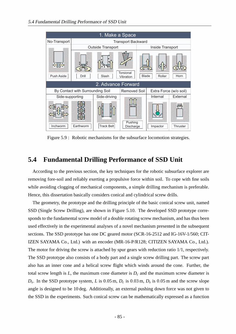
5.4 Fundamental Drilling Performance of SSD Unit
No-Transport Transport Backward
Outside Transport Inside Transport
Push Aside Drill SlashTorsional
Vibration Blade Roller Horn
1. Make a Space
2. Advance Forward
By Contact with Surrounding Soil Removed Soil
Pushing
Discharge
Extra Force (w/o soil)
Side-supporting Side-driving Internal External
Track BeltEarthwormInchworm Impactor Thruster
Figure 5.9 : Robotic mechanisms for the subsurface locomotion strategies.
5.4 Fundamental Drilling Performance of SSD Unit
According to the previous section, the key techniques for the robotic subsurface explorer are
removing fore-soil and reliably exerting a propulsive force within soil. To cope with fine soils
while avoiding clogging of mechanical components, a simple drilling mechanism is preferable.
Hence, this dissertation basically considers conical and cylindrical screw drills.
The geometry, the prototype and the drilling principle of the basic conical screw unit, named
SSD (Single Screw Drilling), are shown in Figure 5.10. The developed SSD prototype corre-
sponds to the fundamental screw model of a double rotating screw mechanism, and has thus been
used effectively in the experimental analyses of a novel mechanism presented in the subsequent
sections. The SSD prototype has one DC geared motor (SCR-16-2512 and IG-16V-1/560; CIT-
IZEN SAYAMA Co., Ltd.) with an encoder (MR-16-P/R128; CITIZEN SAYAMA Co., Ltd.).
The motor for driving the screw is attached by spur gears with reduction ratio 1/1, respectively.
The SSD prototype also consists of a body part and a single screw drilling part. The screw part
also has an inner cone and a helical screw flight which winds around the cone. Further, the
total screw length isL, the maximum cone diameter isDc and the maximum screw diameter is
Ds. In the SSD prototype system,L is 0.05m, Dc is 0.03m, Ds is 0.05m and the screw slope
angle is designed to be10deg. Additionally, an external pushing down force was not given to
the SSD in the experiments. Such conical screw can be mathematically expressed as a function
- 85 -
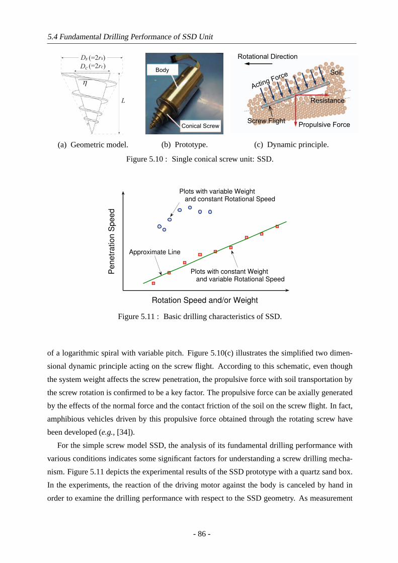
5.4 Fundamental Drilling Performance of SSD Unit
(=2rs)
(=2rc)
(a) Geometric model.
Body
Conical Screw
(b) Prototype.
Rotational Direction
Soil
Screw Flight
Acting Force
Propulsive Force
Resistance
(c) Dynamic principle.
Figure 5.10 : Single conical screw unit: SSD.
Rotation Speed and/or Weight
Penetr
ation S
peed
Approximate Line
Plots with variable Weight
and constant Rotational Speed
Plots with constant Weight
and variable Rotational Speed
Figure 5.11 : Basic drilling characteristics of SSD.
of a logarithmic spiral with variable pitch. Figure 5.10(c) illustrates the simplified two dimen-
sional dynamic principle acting on the screw flight. According to this schematic, even though
the system weight affects the screw penetration, the propulsive force with soil transportation by
the screw rotation is confirmed to be a key factor. The propulsive force can be axially generated
by the effects of the normal force and the contact friction of the soil on the screw flight. In fact,
amphibious vehicles driven by this propulsive force obtained through the rotating screw have
been developed (e.g., [34]).
For the simple screw model SSD, the analysis of its fundamental drilling performance with
various conditions indicates some significant factors for understanding a screw drilling mecha-
nism. Figure 5.11 depicts the experimental results of the SSD prototype with a quartz sand box.
In the experiments, the reaction of the driving motor against the body is canceled by hand in
order to examine the drilling performance with respect to the SSD geometry. As measurement
- 86 -
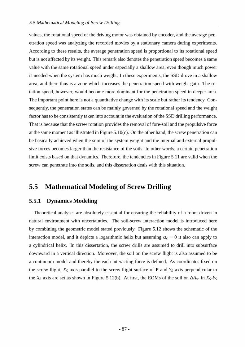
5.5 Mathematical Modeling of Screw Drilling
values, the rotational speed of the driving motor was obtained by encoder, and the average pen-
etration speed was analyzing the recorded movies by a stationary camera during experiments.
According to these results, the average penetration speed is proportional to its rotational speed
but is not affected by its weight. This remark also denotes the penetration speed becomes a same
value with the same rotational speed under especially a shallow area, even though much power
is needed when the system has much weight. In these experiments, the SSD drove in a shallow
area, and there thus is a zone which increases the penetration speed with weight gain. The ro-
tation speed, however, would become more dominant for the penetration speed in deeper area.
The important point here is not a quantitative change with its scale but rather its tendency. Con-
sequently, the penetration states can be mainly governed by the rotational speed and the weight
factor has to be consistently taken into account in the evaluation of the SSD drilling performance.
That is because that the screw rotation provides the removal of fore-soil and the propulsive force
at the same moment as illustrated in Figure 5.10(c). On the other hand, the screw penetration can
be basically achieved when the sum of the system weight and the internal and external propul-
sive forces becomes larger than the resistance of the soils. In other words, a certain penetration
limit exists based on that dynamics. Therefore, the tendencies in Figure 5.11 are valid when the
screw can penetrate into the soils, and this dissertation deals with this situation.
5.5 Mathematical Modeling of Screw Drilling
5.5.1 Dynamics Modeling
Theoretical analyses are absolutely essential for ensuring the reliability of a robot driven in
natural environment with uncertainties. The soil-screw interaction model is introduced here
by combining the geometric model stated previously. Figure 5.12 shows the schematic of the
interaction model, and it depicts a logarithmic helix but assumingαc = 0 it also can apply to
a cylindrical helix. In this dissertation, the screw drills are assumed to drill into subsurface
downward in a vertical direction. Moreover, the soil on the screw flight is also assumed to be
a continuum model and thereby the each interacting force is defined. As coordinates fixed on
the screw flight,XS axis parallel to the screw flight surface ofP andYS axis perpendicular to
theXS axis are set as shown in Figure 5.12(b). At first, the EOMs of the soil on∆Asc in XS-YS
- 87 -
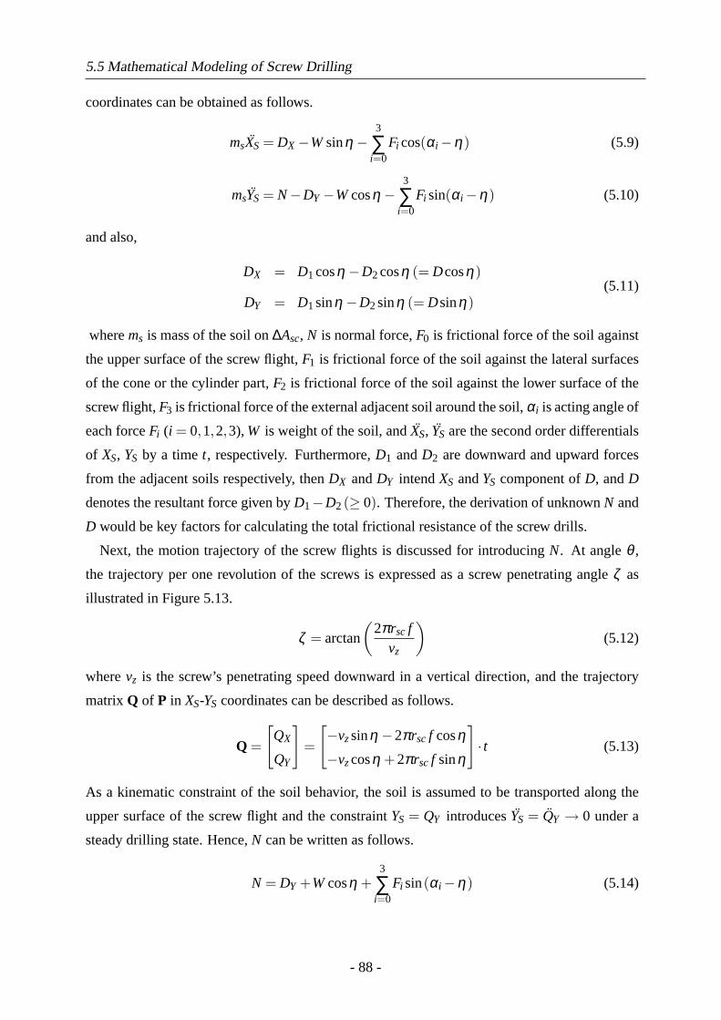
5.5 Mathematical Modeling of Screw Drilling
coordinates can be obtained as follows.
msXS = DX−Wsinη−3
∑i=0
Fi cos(αi−η) (5.9)
msYS = N−DY−Wcosη−3
∑i=0
Fi sin(αi−η) (5.10)
and also,
DX = D1cosη−D2cosη (= Dcosη)
DY = D1sinη−D2sinη (= Dsinη)(5.11)
wherems is mass of the soil on∆Asc, N is normal force,F0 is frictional force of the soil against
the upper surface of the screw flight,F1 is frictional force of the soil against the lateral surfaces
of the cone or the cylinder part,F2 is frictional force of the soil against the lower surface of the
screw flight,F3 is frictional force of the external adjacent soil around the soil,αi is acting angle of
each forceFi (i = 0,1,2,3), W is weight of the soil, andXS, YS are the second order differentials
of XS, YS by a timet, respectively. Furthermore,D1 andD2 are downward and upward forces
from the adjacent soils respectively, thenDX andDY intendXS andYS component ofD, andD
denotes the resultant force given byD1−D2(≥ 0). Therefore, the derivation of unknownN and
D would be key factors for calculating the total frictional resistance of the screw drills.
Next, the motion trajectory of the screw flights is discussed for introducingN. At angleθ ,
the trajectory per one revolution of the screws is expressed as a screw penetrating angleζ as
illustrated in Figure 5.13.
ζ = arctan
(2πrscf
vz
)(5.12)
wherevz is the screw’s penetrating speed downward in a vertical direction, and the trajectory
matrix Q of P in XS-YS coordinates can be described as follows.
Q =
[QX
QY
]=
[−vzsinη−2πrscf cosη−vzcosη +2πrscf sinη
]· t (5.13)
As a kinematic constraint of the soil behavior, the soil is assumed to be transported along the
upper surface of the screw flight and the constraintYS = QY introducesYS = QY → 0 under a
steady drilling state. Hence,N can be written as follows.
N = DY +Wcosη +3
∑i=0
Fi sin(αi−η) (5.14)
- 88 -
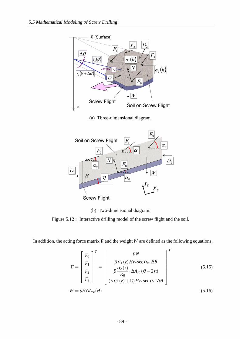
5.5 Mathematical Modeling of Screw Drilling
(a) Three-dimensional diagram.
(b) Two-dimensional diagram.
Figure 5.12 : Interactive drilling model of the screw flight and the soil.
In addition, the acting force matrixF and the weightW are defined as the following equations.
F =
F0
F1
F2
F3
T
=
µN
µσ1(z)Hrcsecαc ·∆θ
µσ2(z)
K0·∆Asc(θ −2π)
(µσ3(z)+C)Hrssecαs ·∆θ
T
(5.15)
W = γH∆Asc(θ) (5.16)
- 89 -
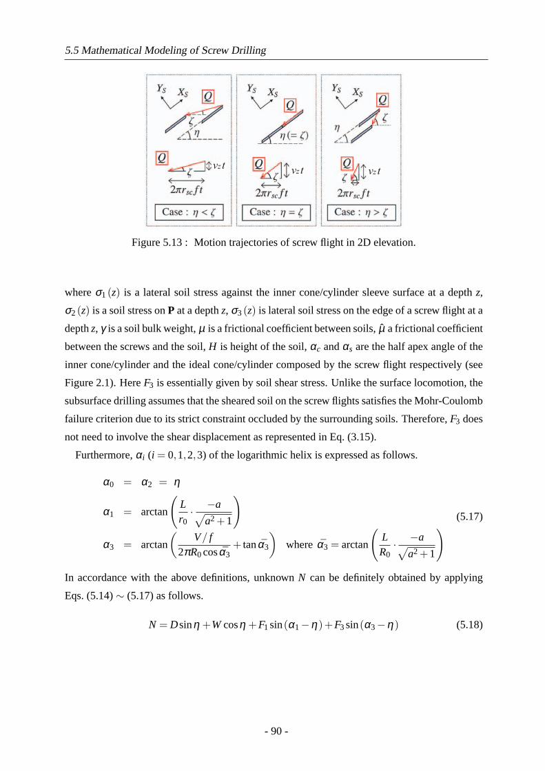
5.5 Mathematical Modeling of Screw Drilling
vz tvz t vz t
Figure 5.13 : Motion trajectories of screw flight in 2D elevation.
whereσ1(z) is a lateral soil stress against the inner cone/cylinder sleeve surface at a depthz,
σ2(z) is a soil stress onP at a depthz, σ3(z) is lateral soil stress on the edge of a screw flight at a
depthz, γ is a soil bulk weight,µ is a frictional coefficient between soils,µ a frictional coefficient
between the screws and the soil,H is height of the soil,αc andαs are the half apex angle of the
inner cone/cylinder and the ideal cone/cylinder composed by the screw flight respectively (see
Figure 2.1). HereF3 is essentially given by soil shear stress. Unlike the surface locomotion, the
subsurface drilling assumes that the sheared soil on the screw flights satisfies the Mohr-Coulomb
failure criterion due to its strict constraint occluded by the surrounding soils. Therefore,F3 does
not need to involve the shear displacement as represented in Eq. (3.15).
Furthermore,αi (i = 0,1,2,3) of the logarithmic helix is expressed as follows.
α0 = α2 = η
α1 = arctan
(Lr0· −a√
a2 +1
)
α3 = arctan
(V/ f
2πR0cosα3+ tanα3
)whereα3 = arctan
(LR0· −a√
a2 +1
)(5.17)
In accordance with the above definitions, unknownN can be definitely obtained by applying
Eqs. (5.14)∼ (5.17) as follows.
N = Dsinη +Wcosη +F1sin(α1−η)+F3sin(α3−η) (5.18)
- 90 -
5.5 Mathematical Modeling of Screw Drilling
Also, the heightH is defined as follows.
2π ≥ θ ≥ 0 =⇒ H =
{h− l : 0≤ θ ≤ 2πp : 2π ≤ θ ≤ θend
(5.19)
2π < θ =⇒ H =
h− l : 0≤ θ ≤ 2πkH
vz
f: 2π ≤ θ ≤ θ
p : θ ≤ θ ≤ θend
(5.20)
whereh is apex depth,θ is angle atp(θ) = vz/ f (however actualθ of the logarithmic helix is de-
rived by Eq. (2.5) as two values,p is assumed to be specific value in the range of2π ≤ θ ≤ θend,
andH is assumed to be equal toh− l in the range of0≤ θ ≤ 2π), kH is an expansion coefficient
of H by a soil flow and its effective range is set to be1≤ kH ≤ p f/vz. When the penetration
speedvz is constant and drilled borehole is assumed to be self-standing,kH can simply become
1.
As the next step, the resultant forceD is introduced. In this dissertation, based on the dy-
namic discharging behavior of soils, the sum of the rotating moment byD is defined as the total
change of potential energy by uplifting the whole soils on a screw flight fromθ = 0 to θ = θend.
Accordingly, the following relation is here given.
∫ θ=θend
θ=0Drsc·dθ =
12π
∫ θ=θend
θ=0WHtanη (5.21)
As a result, the total frictional resistance momentMT , acting from the soil on the screw flights,
can be calculated as follows.
MT =∫ θ=θend
θ=0(∆MN +∆MF) (5.22)
and also,
∆MN = Nrscsinη (5.23)
∆MF = F · r (5.24)
r =[rsccosα0 rccosα1 exp(2aπ) rsccosα2 0
]T(5.25)
z= h− l − H2
(5.26)
wherer is coefficient matrix ofF for converting into torques andz is corresponding depth for
each soil stress defined in Eq. (5.15).
- 91 -
5.5 Mathematical Modeling of Screw Drilling
5.5.2 Cavity Expansion Theory
In the light of soil mechanics, soil pressure is basically composed of the weight and the co-
hesion of soils [102, 109]. Previously, the soil resistances were defined as the friction by the
interactive contact forces. However, the effect of compressing soil by the screw penetration is
actually needed to be included inσ1(z), σ2(z) andσ3(z) for practical estimation. So this research
attempts to apply a cavity expansion theory [105,108] to the soil-screw interaction model.
Generally, the cavity expansion theory has been applied in order to evaluate the bearing capac-
ity of a pile penetrating into the ground. This theory is one of the few elastic-plastic problems
which can be solved analytically. Here the soil model is represented as a Mohr-Coulomb’s
elasto-plastic solid as shown in Figure 5.14, and a cylindrical cavity expansion is assumed. The
problem is defined that the diameter of the soil cavity is firstlyrz, and then the diameter is ex-
panded toRz by applying external forces. Further, the distance of an elasto-plastic boundary
from the center position,Re, is set to be expanded with the displacement of the soil in an elastic
zone,dUe. Also, a distance from the center position is defined asr, andψ is set to be a angle
direction normal tor. Each stress component alongr andψ, σr andσψ , is principal stress due to
the symmetrical property of the cavity. Therefore, the relation betweenσr andσψ in the elastic
zone can be defined as the following failure criteria equation of soils.
σr −σψ = (σr +σψ)sinφ +2Ccosφ (5.27)
whereφ is internal friction angle andC is cohesion.
For the plastic and the elastic zones of the subsurface soil, the following equilibrium equations
of the cylindrical stresses can be given by
· Plastic Zone:
∂σr
∂ r+
σr −σψ
r= 0 (5.28)
· Elastic Zone:
σr = C1 +C2
r2 , σψ = C1−C2
r2 (5.29)
whereC1 andC2 are integration constants.
Given a boundary condition, the soil stress atr = ∞ is assumed to be a static soil pressure of an
isotropic elastic medium,σr = σψ = K0γz (whereK0 is a coefficient of lateral soil pressure and
γ is a soil bulk weight density). Therefore,C1 = K0γz can be determined. At the elastic-plastic
boundary (i.e.r = Re), C2 = R2e(K0γzsinφ +Ccosφ) can be derived from Eqs. (5.27) and (5.29).
- 92 -
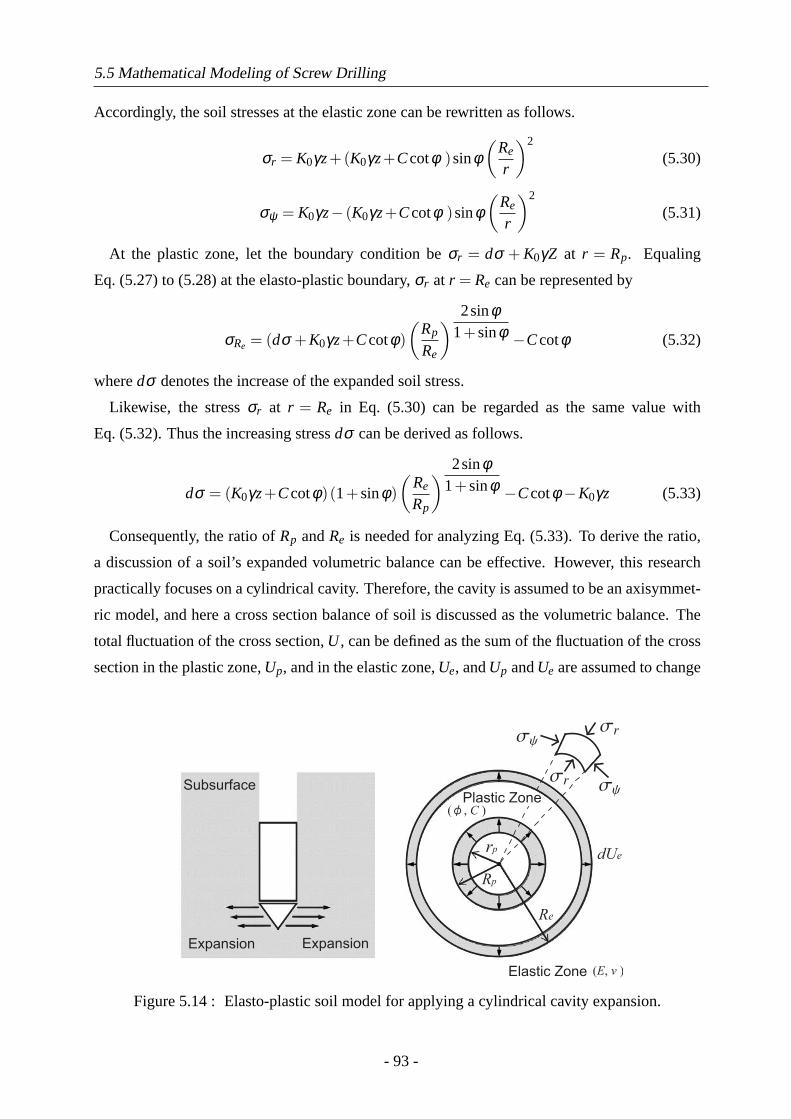
5.5 Mathematical Modeling of Screw Drilling
Accordingly, the soil stresses at the elastic zone can be rewritten as follows.
σr = K0γz+(K0γz+Ccotφ )sinφ(
Re
r
)2
(5.30)
σψ = K0γz− (K0γz+Ccotφ )sinφ(
Re
r
)2
(5.31)
At the plastic zone, let the boundary condition beσr = dσ + K0γZ at r = Rp. Equaling
Eq. (5.27) to (5.28) at the elasto-plastic boundary,σr at r = Re can be represented by
σRe = (dσ +K0γz+Ccotφ)(
Rp
Re
) 2sinφ1+sinφ −Ccotφ (5.32)
wheredσ denotes the increase of the expanded soil stress.
Likewise, the stressσr at r = Re in Eq. (5.30) can be regarded as the same value with
Eq. (5.32). Thus the increasing stressdσ can be derived as follows.
dσ = (K0γz+Ccotφ)(1+sinφ)(
Re
Rp
) 2sinφ1+sinφ −Ccotφ −K0γz (5.33)
Consequently, the ratio ofRp andRe is needed for analyzing Eq. (5.33). To derive the ratio,
a discussion of a soil’s expanded volumetric balance can be effective. However, this research
practically focuses on a cylindrical cavity. Therefore, the cavity is assumed to be an axisymmet-
ric model, and here a cross section balance of soil is discussed as the volumetric balance. The
total fluctuation of the cross section,U , can be defined as the sum of the fluctuation of the cross
section in the plastic zone,Up, and in the elastic zone,Ue, andUp andUe are assumed to change
Subsurface
Expansion Expansion
Elastic Zone
Plastic Zone
Figure 5.14 : Elasto-plastic soil model for applying a cylindrical cavity expansion.
- 93 -
5.5 Mathematical Modeling of Screw Drilling
independently. By reference to Figure 5.14, the balance can be expressed by
U = Up +Ue (5.34)
ans also,
U = R2p− r2
p (5.35)
Up =(R2
e−R2p
)∆ (5.36)
Ue = R2e− (Re−dUe)
2 (5.37)
dUe =1+ν
E(K0γz+Ccotφ)sinφRe = C3Re (5.38)
where∆ is an average change ratio of expanding cross section in the plastic zone,ν is Poisson’s
ratio,E is Young’s modulus. DisplacementdUe is provided by integrating the above Eq. (5.30),
and here the volumetric force of soil is assumed to be neglected. Accordingly, the following
equations can be derived by analyzing the volumetric balance.
rp = Rp
(rc
rc +q
)= Rpξ (5.39)
q =vz
ftanαc (5.40)
From the above definitions,ξ satisfiesξ ≤ 1.
Re
Rp=
(1+∆−ξ 2
1+∆− (C3−1)2
)12
(5.41)
Here Eq. (5.41) must satisfy the following conditional equation derived by the inequality
constraintRe > Rp, which intends the existence of a plastic zone.
0≤ ξ (θ) < |C3−1| ≤ 1 (5.42)
Based on the remarks as described above,σ1(z) including the cavity expansion effect can be
estimated as follows.
σ1(z) = dσ +K0γz
= (K0γz+Ccotφ)(1+sinφ)[
1+∆−ξ 2
1+∆− (C3−1)2
] sinφ1+sinφ −Ccotφ (5.43)
- 94 -
5.6 Experimental Evaluation
Furthermore, bothσ2(z) at r = rsc(θ +2π) andσ3(z) at r = rs can be computed by stresses in
a plastic zone as the following equation.
[σ2(z)
σ3(z)
]= (dσ +K0γz+Ccotφ)
(r0
R
) 2sinφ1+sinφ
(r0
R0
) 2sinφ1+sinφ
−Ccotφ (5.44)
5.5.3 Parametric Analysis
To discuss characteristics of the model, parametric analyses were conducted by numerical
simulations. As simulated soil environment, quartz sand was assumed. The nominal property
of the Lunarant was:φ = 33deg,C = 0Pa, ρ = 1523kg/m3 (γ = ρg), K0 = 0.5, ∆ = 0.03,
ν = 0.4, E = 1.0× 10⁶ Pa andµ = 0.5. The nominal parameters were basically determined
based on the reference data of quartz sand [106]. Further, screw geometric and kinematic param-
eters were determined based on the SSD:L = 0.05m, r0 = 0.015m, R0 = 0.025m, η = 10deg,
θend= 15π rad,vz = 0.002m/s, f = 0.2rev/s,kH = 1 andh = 0.5m.
Figure 5.15 plots the simulation results. From Figure 5.15(a), a tendency of whichMT in-
creases as the square ofh was confirmed. On the other hand, Figure 5.15(b) indicated thatMT
decreases with an increase ofη . Increasingη , however, yields depression of the propulsive
force. Thus proper design of the screw, meeting mission requirements, will become a signifi-
cant factor. Additionally, Figures 5.15(c) and 5.15(d) depict the effects of the soil parameters
on MT . According to these graphs,C and∆ greatly influenceMT , while φ and(1+ ν)/E have
a relatively small effect onMT . In particular,∆ is the most influential parameter but is a diffi-
cult parameter to be identified. Therefore, in actual unmanned missions, it will be a valuable
technique to ensure the screw’s performance under estimated parameter range.
5.6 Experimental Evaluation
5.6.1 Experimental Methodology
The drilling experiment of the SSD has been conducted to compare with simulation result.
The experimental overview is shown in Figure 5.16 The target soil is quartz sand (no.5), fly ash
and the Lunarant. The Lunarant is is one of lunar soil simulant and consists of fine particles and
is produced by WEL RESEARCH Co., Ltd. [110]. The property of the test soils are shown in
Figure 5.17 and Table 5.6. The starting situation is that the screw is completely buried and the
- 95 -
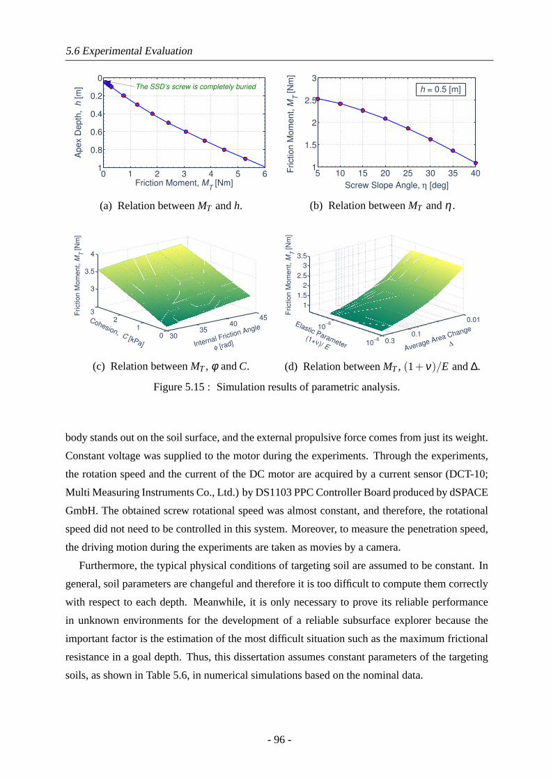
5.6 Experimental Evaluation
0 1 2 3 4 5 6
0
0.2
0.4
0.6
0.8
1
Friction Moment, MT [Nm]
Apex D
epth
, h
[m
] The SSD’s screw is completely buried
(a) Relation betweenMT andh.
5 10 15 20 25 30 35 401
1.5
2
2.5
3
Screw Slope Angle, η [deg]
Friction M
om
ent, M
T [N
m]
h = 0.5 [m]
(b) Relation betweenMT andη .
3035
4045
0
1
2
3
3
3.5
4
Internal Friction Angle
φ [rad]
Cohesion, C [kPa]
Frictio
n M
om
en
t, M
T [
Nm
]
(c) Relation betweenMT , φ andC.
10−8
10−6
0.01
0.1
0.3
1
1.5
2
2.5
3
3.5
Average Area Change
∆
Elastic Parameter
(1+ν)/ E
Frictio
n M
om
en
t, M
T [
Nm
]
(d) Relation betweenMT , (1+ν)/E and∆.
Figure 5.15 : Simulation results of parametric analysis.
body stands out on the soil surface, and the external propulsive force comes from just its weight.
Constant voltage was supplied to the motor during the experiments. Through the experiments,
the rotation speed and the current of the DC motor are acquired by a current sensor (DCT-10;
Multi Measuring Instruments Co., Ltd.) by DS1103 PPC Controller Board produced by dSPACE
GmbH. The obtained screw rotational speed was almost constant, and therefore, the rotational
speed did not need to be controlled in this system. Moreover, to measure the penetration speed,
the driving motion during the experiments are taken as movies by a camera.
Furthermore, the typical physical conditions of targeting soil are assumed to be constant. In
general, soil parameters are changeful and therefore it is too difficult to compute them correctly
with respect to each depth. Meanwhile, it is only necessary to prove its reliable performance
in unknown environments for the development of a reliable subsurface explorer because the
important factor is the estimation of the most difficult situation such as the maximum frictional
resistance in a goal depth. Thus, this dissertation assumes constant parameters of the targeting
soils, as shown in Table 5.6, in numerical simulations based on the nominal data.
- 96 -
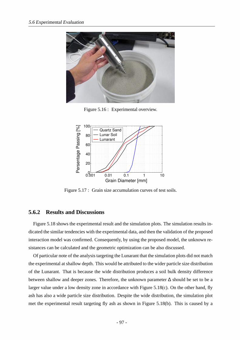
5.6 Experimental Evaluation
Figure 5.16 : Experimental overview.
0.001 0.01 0.1 1 100
20
40
60
80
100
Grain Diameter [mm]
Pers
enta
ge P
assin
g [%
]
Quartz Sand
Lunar Soil
Lunarant
Figure 5.17 : Grain size accumulation curves of test soils.
5.6.2 Results and Discussions
Figure 5.18 shows the experimental result and the simulation plots. The simulation results in-
dicated the similar tendencies with the experimental data, and then the validation of the proposed
interaction model was confirmed. Consequently, by using the proposed model, the unknown re-
sistances can be calculated and the geometric optimization can be also discussed.
Of particular note of the analysis targeting the Lunarant that the simulation plots did not match
the experimental at shallow depth. This would be attributed to the wider particle size distribution
of the Lunarant. That is because the wide distribution produces a soil bulk density difference
between shallow and deeper zones. Therefore, the unknown parameter∆ should be set to be a
larger value under a low density zone in accordance with Figure 5.18(c). On the other hand, fly
ash has also a wide particle size distribution. Despite the wide distribution, the simulation plot
met the experimental result targeting fly ash as shown in Figure 5.18(b). This is caused by a
- 97 -
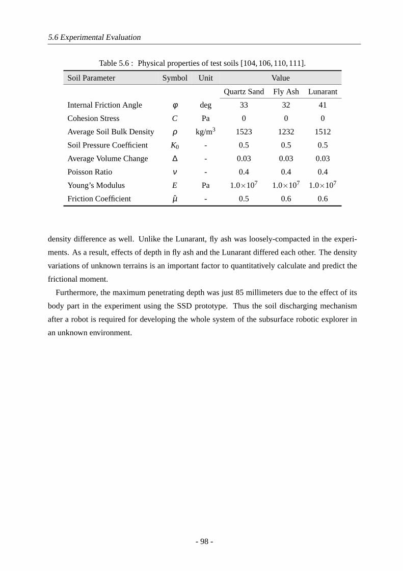
5.6 Experimental Evaluation
Table 5.6 : Physical properties of test soils [104,106,110,111].
Soil Parameter Symbol Unit Value
Quartz Sand Fly Ash Lunarant
Internal Friction Angle φ deg 33 32 41
Cohesion Stress C Pa 0 0 0
Average Soil Bulk Density ρ kg/m3 1523 1232 1512
Soil Pressure Coefficient K0 - 0.5 0.5 0.5
Average Volume Change ∆ - 0.03 0.03 0.03
Poisson Ratio ν - 0.4 0.4 0.4
Young’s Modulus E Pa 1.0×10⁷ 1.0×10⁷ 1.0×10⁷
Friction Coefficient µ - 0.5 0.6 0.6
density difference as well. Unlike the Lunarant, fly ash was loosely-compacted in the experi-
ments. As a result, effects of depth in fly ash and the Lunarant differed each other. The density
variations of unknown terrains is an important factor to quantitatively calculate and predict the
frictional moment.
Furthermore, the maximum penetrating depth was just 85 millimeters due to the effect of its
body part in the experiment using the SSD prototype. Thus the soil discharging mechanism
after a robot is required for developing the whole system of the subsurface robotic explorer in
an unknown environment.
- 98 -
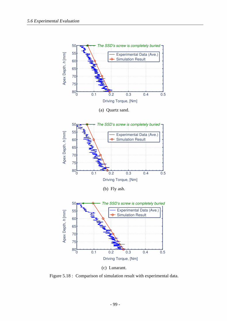
5.6 Experimental Evaluation
0 0.1 0.2 0.3 0.4 0.5
50
55
60
65
70
75
80
Driving Torque, [Nm]
Ap
ex D
ep
th, h [
mm
]
Experimental Data (Ave.)
Simulation Result
The SSD’s screw is completely buried
(a) Quartz sand.
0 0.1 0.2 0.3 0.4 0.5
50
55
60
65
70
75
80
Driving Torque, [Nm]
Ap
ex D
ep
th, h [
mm
]
Experimental Data (Ave.)
Simulation Result
The SSD’s screw is completely buried
(b) Fly ash.
0 0.1 0.2 0.3 0.4 0.5
50
55
60
65
70
75
80
Driving Torque, [Nm]
Ap
ex D
ep
th, h [
mm
]
Experimental Data (Ave.)
Simulation Result
The SSD’s screw is completely buried
(c) Lunarant.
Figure 5.18 : Comparison of simulation result with experimental data.
- 99 -
5.7 Summary
5.7 Summary
Firstly, this chapter presented the requirements and the locomotion strategy for a subsurface
robotic explorer on the Moon. Then a novel soil-screw interaction model for the subsurface
locomotion was proposed. The characteristics of the developed model were evaluated by para-
metric analyses. These analyses indicated the influence of various parameters on the frictional
moment. As a result, key parameters could be determined for the subsurface locomotion. The
main contributions of this chapter is the derivation of the screw’s dynamics model based upon
soil mechanics with the cavity expansion theory. Such detailed model is unprecedented and
provides crucial ideas adaptable to general screw mechanism. Also, the theoretical approach
enables to optimize the geometric design of the screw. This will be a significant guideline for
space applications, targeting unknown environment.
- 100 -
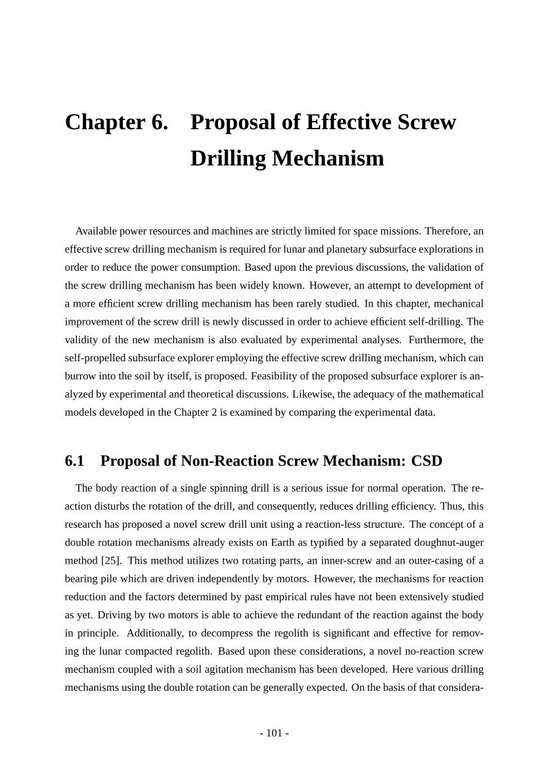
Chapter 6. Proposal of Effective Screw
Drilling Mechanism
Available power resources and machines are strictly limited for space missions. Therefore, an
effective screw drilling mechanism is required for lunar and planetary subsurface explorations in
order to reduce the power consumption. Based upon the previous discussions, the validation of
the screw drilling mechanism has been widely known. However, an attempt to development of
a more efficient screw drilling mechanism has been rarely studied. In this chapter, mechanical
improvement of the screw drill is newly discussed in order to achieve efficient self-drilling. The
validity of the new mechanism is also evaluated by experimental analyses. Furthermore, the
self-propelled subsurface explorer employing the effective screw drilling mechanism, which can
burrow into the soil by itself, is proposed. Feasibility of the proposed subsurface explorer is an-
alyzed by experimental and theoretical discussions. Likewise, the adequacy of the mathematical
models developed in the Chapter 2 is examined by comparing the experimental data.
6.1 Proposal of Non-Reaction Screw Mechanism: CSD
The body reaction of a single spinning drill is a serious issue for normal operation. The re-
action disturbs the rotation of the drill, and consequently, reduces drilling efficiency. Thus, this
research has proposed a novel screw drill unit using a reaction-less structure. The concept of a
double rotation mechanisms already exists on Earth as typified by a separated doughnut-auger
method [25]. This method utilizes two rotating parts, an inner-screw and an outer-casing of a
bearing pile which are driven independently by motors. However, the mechanisms for reaction
reduction and the factors determined by past empirical rules have not been extensively studied
as yet. Driving by two motors is able to achieve the redundant of the reaction against the body
in principle. Additionally, to decompress the regolith is significant and effective for remov-
ing the lunar compacted regolith. Based upon these considerations, a novel no-reaction screw
mechanism coupled with a soil agitation mechanism has been developed. Here various drilling
mechanisms using the double rotation can be generally expected. On the basis of that considera-
- 101 -
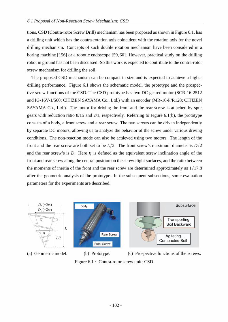
6.1 Proposal of Non-Reaction Screw Mechanism: CSD
tions, CSD (Contra-rotor Screw Drill) mechanism has been proposed as shown in Figure 6.1, has
a drilling unit which has the contra-rotation axis coincident with the rotation axis for the novel
drilling mechanism. Concepts of such double rotation mechanism have been considered in a
boring machine [156] or a robotic endoscope [59, 60]. However, practical study on the drilling
robot in ground has not been discussed. So this work is expected to contribute to the contra-rotor
screw mechanism for drilling the soil.
The proposed CSD mechanism can be compact in size and is expected to achieve a higher
drilling performance. Figure 6.1 shows the schematic model, the prototype and the prospec-
tive screw functions of the CSD. The CSD prototype has two DC geared motor (SCR-16-2512
and IG-16V-1/560; CITIZEN SAYAMA Co., Ltd.) with an encoder (MR-16-P/R128; CITIZEN
SAYAMA Co., Ltd.). The motor for driving the front and the rear screw is attached by spur
gears with reduction ratio 8/15 and 2/1, respectively. Referring to Figure 6.1(b), the prototype
consists of a body, a front screw and a rear screw. The two screws can be driven independently
by separate DC motors, allowing us to analyze the behavior of the screw under various driving
conditions. The non-reaction mode can also be achieved using two motors. The length of the
front and the rear screw are both set to beL/2. The front screw’s maximum diameter isD/2
and the rear screw’s isD. Hereη is defined as the equivalent screw inclination angle of the
front and rear screw along the central position on the screw flight surfaces, and the ratio between
the moments of inertia of the front and the rear screw are determined approximately as1/17.8
after the geometric analysis of the prototype. In the subsequent subsections, some evaluation
parameters for the experiments are described.
(=2rs)
(=2rc)
(a) Geometric model.
Body
Rear Screw
Front Screw
(b) Prototype.
Subsurface
Transporting
Soil Backward
Agitating
Compacted Soil
(c) Prospective functions of the screws.
Figure 6.1 : Contra-rotor screw unit: CSD.
- 102 -
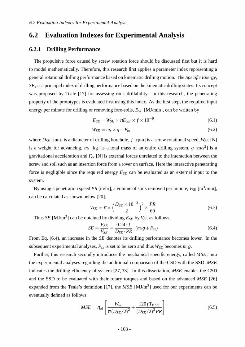
6.2 Evaluation Indexes for Experimental Analysis
6.2 Evaluation Indexes for Experimental Analysis
6.2.1 Drilling Performance
The propulsive force caused by screw rotation force should be discussed first but it is hard
to model mathematically. Therefore, this research first applies a parameter index representing a
general rotational drilling performance based on kinematic drilling motion. TheSpecific Energy,
SE, is a principal index of drilling performance based on the kinematic drilling states. Its concept
was proposed by Teale [17] for assessing rock drillability. In this research, the penetrating
property of the prototypes is evaluated first using this index. As the first step, the required input
energy per minute for drilling or removing fore-soils,ESE [MJ/min], can be written by
ESE = WSE×πDSE× f ×10−9 (6.1)
WSE = mr ×g+Fex (6.2)
whereDSE [mm] is a diameter of drilling borehole,f [rpm] is a screw rotational speed,WSE [N]
is a weight for advancing,mr [kg] is a total mass of an entire drilling system,g [m/s2] is a
gravitational acceleration andFex [N] is external forces unrelated to the interaction between the
screw and soil such as an insertion force from a rover on surface. Here the interactive penetrating
force is negligible since the required energyESE can be evaluated as an external input to the
system.
By using a penetration speedPR[m/hr], a volume of soils removed per minute,VSE [m3/min],
can be calculated as shown below [20].
VSE = π×(DSE×10−3
2
)2× PR
60(6.3)
ThusSE [MJ/m3] can be obtained by dividingESE by VSE as follows.
SE=ESE
VSE=
0.24· fDSE·PR
· (mrg+Fex) (6.4)
From Eq. (6.4), an increase in theSE denotes its drilling performance becomes lower. In the
subsequent experimental analyses,Fex is set to be zero and thusWSE becomesmrg.
Further, this research secondly introduces the mechanical specific energy, calledMSE, into
the experimental analyses regarding the additional comparison of the CSD with the SSD.MSE
indicates the drilling efficiency of system [27, 33]. In this dissertation,MSE enables the CSD
and the SSD to be evaluated with their rotary torques and based on the advancedMSE [26]
expanded from the Teale’s definition [17], theMSE [MJ/m3] used for our experiments can be
eventually defined as follows.
MSE= ηM
[WSE
π (DSE/2)2 +120f TMSE
(DSE/2)2PR
](6.5)
- 103 -
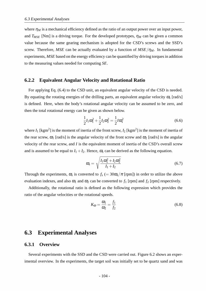
6.3 Experimental Analyses
whereηM is a mechanical efficiency defined as the ratio of an output power over an input power,
andTMSE [Nm] is a driving torque. For the developed prototypes,ηM can be given a common
value because the same gearing mechanism is adopted for the CSD’s screws and the SSD’s
screw. Therefore,MSE can be actually evaluated by a function ofMSE/ηM. In fundamental
experiments,MSEbased on the energy efficiency can be quantified by driving torques in addition
to the measuring values needed for computingSE.
6.2.2 Equivalent Angular Velocity and Rotational Ratio
For applying Eq. (6.4) to the CSD unit, an equivalent angular velocity of the CSD is needed.
By equating the rotating energies of the drilling parts, an equivalent angular velocityωs [rad/s]
is defined. Here, when the body’s rotational angular velocity can be assumed to be zero, and
then the total rotational energy can be given as shown below.
12
I1ω21 +
12
I2ω22 =
12
Iω2s (6.6)
whereI1 [kgm2] is the moment of inertia of the front screw,I2 [kgm2] is the moment of inertia of
the rear screw,ω1 [rad/s] is the angular velocity of the front screw andω2 [rad/s] is the angular
velocity of the rear screw, andI is the equivalent moment of inertia of the CSD’s overall screw
and is assumed to be equal toI1 + I2. Hence,ωs can be derived as the following equation.
ωs =
√I1ω2
1 + I2ω22
I1 + I2(6.7)
Through the experiments,ωs is converted tofs (= 30ωs/π [rpm]) in order to utilize the above
evaluation indexes, and alsoω1 andω2 can be converted tof1 [rpm] and f2 [rpm] respectively.
Additionally, the rotational ratio is defined as the following expression which provides the
ratio of the angular velocities or the rotational speeds.
Kω =ω1
ω2=
f1f2
(6.8)
6.3 Experimental Analyses
6.3.1 Overview
Several experiments with the SSD and the CSD were carried out. Figure 6.2 shows an exper-
imental overview. In the experiments, the target soil was initially set to be quartz sand and was
- 104 -
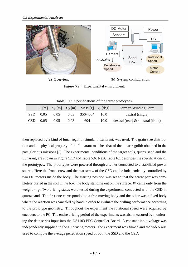
6.3 Experimental Analyses
(a) Overview.
PC
PowerDC Motor
Sensors
CameraSand
BoxPenetration
Speed Motor
Current
Rotational
SpeedAnalyzing
(b) System configuration.
Figure 6.2 : Experimental environment.
Table 6.1 : Specifications of the screw prototypes.
L [m] Ds [m] Dc [m] Mass [g] η [deg] Screw’s Winding Form
SSD 0.05 0.05 0.03 356∼604 10.0 dextral (single)
CSD 0.05 0.05 0.03 604 10.0 dextral (rear) & sinistral (front)
then replaced by a kind of lunar regolith simulant, Lunarant, was used. The grain size distribu-
tion and the physical property of the Lunarant matches that of the lunar regolith obtained in the
past glorious missions [3]. The experimental conditions of the target soils, quartz sand and the
Lunarant, are shown in Figure 5.17 and Table 5.6. Next, Table 6.1 describes the specifications of
the prototypes. The prototypes were powered through a tether connected to a stabilized power
source. Here the front screw and the rear screw of the CSD can be independently controlled by
two DC motors inside the body. The starting position was set so that the screw part was com-
pletely buried in the soil in the box, the body standing out on the surface.W came only from the
weightmrg. Two driving states were tested during the experiments conducted with the CSD in
quartz sand. The first one corresponded to a free moving body and the other was a fixed body
where the reaction was canceled by hand in order to evaluate the drilling performance according
to the prototype geometry. Throughout the experiment the rotational speed were acquired by
encoders to the PC. The entire driving period of the experiments was also measured by monitor-
ing the data series input into the DS1103 PPC Controller Board. A constant input voltage was
independently supplied to the all driving motors. The experiment was filmed and the video was
used to compute the average penetration speed of both the SSD and the CSD.
- 105 -
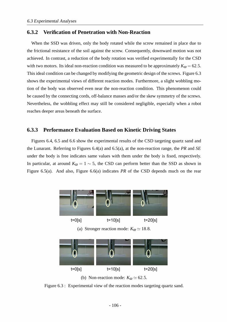
6.3 Experimental Analyses
6.3.2 Verification of Penetration with Non-Reaction
When the SSD was driven, only the body rotated while the screw remained in place due to
the frictional resistance of the soil against the screw. Consequently, downward motion was not
achieved. In contrast, a reduction of the body rotation was verified experimentally for the CSD
with two motors. Its ideal non-reaction condition was measured to be approximatelyKω = 62.5.
This ideal condition can be changed by modifying the geometric design of the screws. Figure 6.3
shows the experimental views of different reaction modes. Furthermore, a slight wobbling mo-
tion of the body was observed even near the non-reaction condition. This phenomenon could
be caused by the connecting cords, off-balance masses and/or the skew symmetry of the screws.
Nevertheless, the wobbling effect may still be considered negligible, especially when a robot
reaches deeper areas beneath the surface.
6.3.3 Performance Evaluation Based on Kinetic Driving States
Figures 6.4, 6.5 and 6.6 show the experimental results of the CSD targeting quartz sand and
the Lunarant. Referring to Figures 6.4(a) and 6.5(a), at the non-reaction range, thePRandSE
under the body is free indicates same values with them under the body is fixed, respectively.
In particular, at aroundKω = 1∼ 5, the CSD can perform better than the SSD as shown in
Figure 6.5(a). And also, Figure 6.6(a) indicatesPR of the CSD depends much on the rear
(a) Stronger reaction mode:Kω ' 18.8.
(b) Non-reaction mode:Kω ' 62.5.
Figure 6.3 : Experimental view of the reaction modes targeting quartz sand.
- 106 -
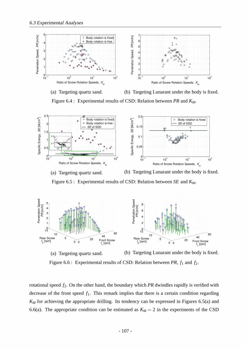
6.3 Experimental Analyses
10−1
100
101
102
0
1
2
3
4
5
Ratio of Screw Rotation Speeds, Kω
Pe
ne
tra
tio
n S
pe
ed
, P
R [
m/h
r]
Body rotation is fixed
Body rotation is free
(a) Targeting quartz sand.
10−1
100
101
102
0
1
2
3
4
5
6
7
Ratio of Screw Rotation Speeds, Kω
Pe
ne
tra
tio
n S
pe
ed
, P
R [
m/h
r]
(b) Targeting Lunarant under the body is fixed.
Figure 6.4 : Experimental results of CSD: Relation betweenPRandKω .
10−1
100
101
102
0
0.5
1
1.5
2
2.5
Ratio of Screw Rotation Speeds, Kω
Sp
ecific
En
erg
y, S
E [
MJ/m
3]
Body rotation is fixed
Body rotation is free
SE of SSD
100
101
0.05
0.1
0.15
0.2
100
101
(a) Targeting quartz sand.
10−1
100
101
102
0
0.05
0.1
0.15
0.2
Ratio of Screw Rotation Speeds, Kω
Sp
ecific
En
erg
y, S
E [
MJ/m
3]
Body rotation is fixed
SE of SSD
(b) Targeting Lunarant under the body is fixed.
Figure 6.5 : Experimental results of CSD: Relation betweenSEandKω .
0
20
40
60
0
5
10
150
1
2
3
4
5
Front Screw
f1 [rpm]
Rear Screw
f2 [rpm]
Pe
ne
tra
tio
n S
pe
ed
PR
[m
/hr]
(a) Targeting quartz sand.
0
20
40
60
0
5
10
150
2
4
6
8
Front Screw
f1 [rpm]
Rear Screw
f2 [rpm]
Pe
ne
tra
tio
n S
pe
ed
PR
[m
/hr]
(b) Targeting Lunarant under the body is fixed.
Figure 6.6 : Experimental results of CSD: Relation betweenPR, f1 and f2.
rotational speedf2. On the other hand, the boundary whichPRdwindles rapidly is verified with
decrease of the front speedf1. This remark implies that there is a certain condition regarding
Kω for achieving the appropriate drilling. Its tendency can be expressed in Figures 6.5(a) and
6.6(a). The appropriate condition can be estimated asKω = 2 in the experiments of the CSD
- 107 -
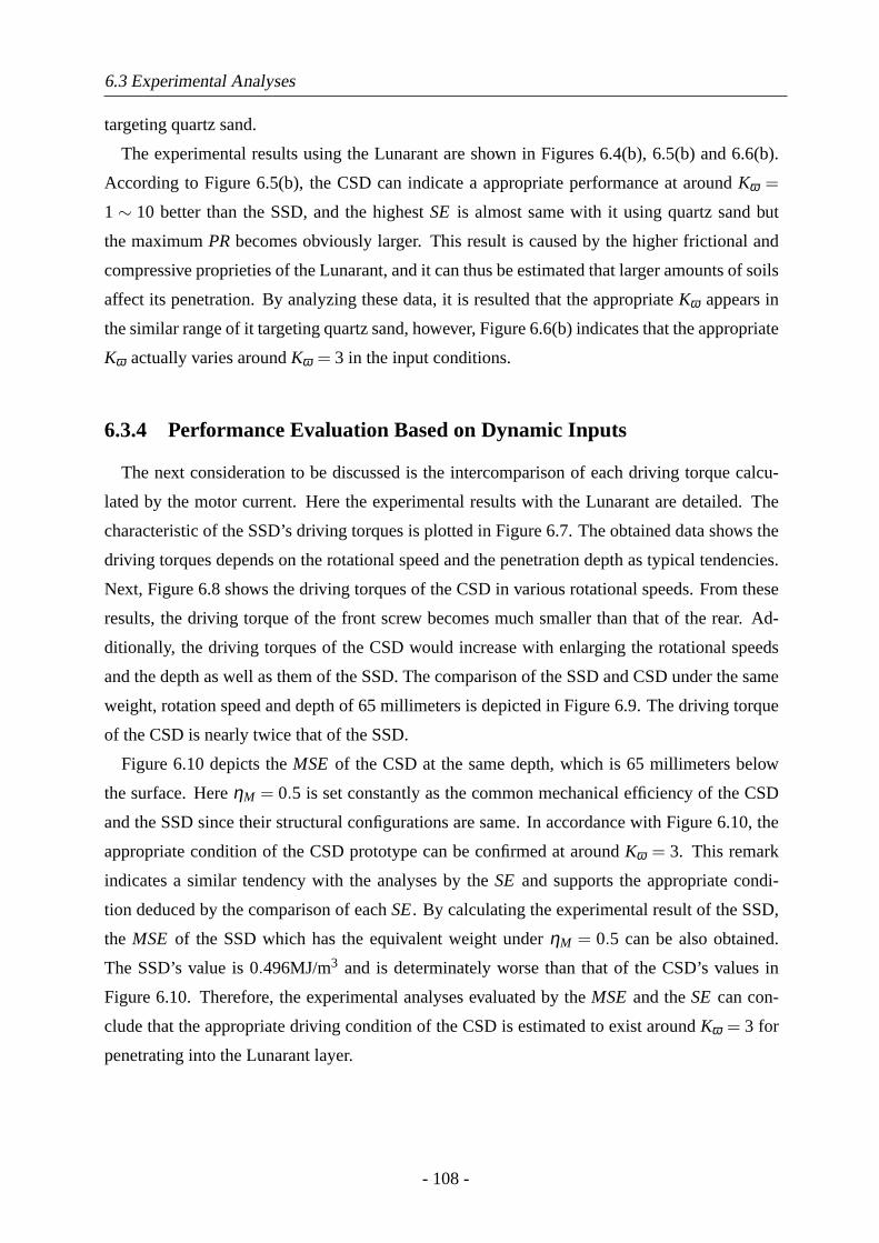
6.3 Experimental Analyses
targeting quartz sand.
The experimental results using the Lunarant are shown in Figures 6.4(b), 6.5(b) and 6.6(b).
According to Figure 6.5(b), the CSD can indicate a appropriate performance at aroundKω =
1∼ 10 better than the SSD, and the highestSE is almost same with it using quartz sand but
the maximumPR becomes obviously larger. This result is caused by the higher frictional and
compressive proprieties of the Lunarant, and it can thus be estimated that larger amounts of soils
affect its penetration. By analyzing these data, it is resulted that the appropriateKω appears in
the similar range of it targeting quartz sand, however, Figure 6.6(b) indicates that the appropriate
Kω actually varies aroundKω = 3 in the input conditions.
6.3.4 Performance Evaluation Based on Dynamic Inputs
The next consideration to be discussed is the intercomparison of each driving torque calcu-
lated by the motor current. Here the experimental results with the Lunarant are detailed. The
characteristic of the SSD’s driving torques is plotted in Figure 6.7. The obtained data shows the
driving torques depends on the rotational speed and the penetration depth as typical tendencies.
Next, Figure 6.8 shows the driving torques of the CSD in various rotational speeds. From these
results, the driving torque of the front screw becomes much smaller than that of the rear. Ad-
ditionally, the driving torques of the CSD would increase with enlarging the rotational speeds
and the depth as well as them of the SSD. The comparison of the SSD and CSD under the same
weight, rotation speed and depth of 65 millimeters is depicted in Figure 6.9. The driving torque
of the CSD is nearly twice that of the SSD.
Figure 6.10 depicts theMSE of the CSD at the same depth, which is 65 millimeters below
the surface. HereηM = 0.5 is set constantly as the common mechanical efficiency of the CSD
and the SSD since their structural configurations are same. In accordance with Figure 6.10, the
appropriate condition of the CSD prototype can be confirmed at aroundKω = 3. This remark
indicates a similar tendency with the analyses by theSE and supports the appropriate condi-
tion deduced by the comparison of eachSE. By calculating the experimental result of the SSD,
the MSE of the SSD which has the equivalent weight underηM = 0.5 can be also obtained.
The SSD’s value is0.496MJ/m3 and is determinately worse than that of the CSD’s values in
Figure 6.10. Therefore, the experimental analyses evaluated by theMSE and theSE can con-
clude that the appropriate driving condition of the CSD is estimated to exist aroundKω = 3 for
penetrating into the Lunarant layer.
- 108 -
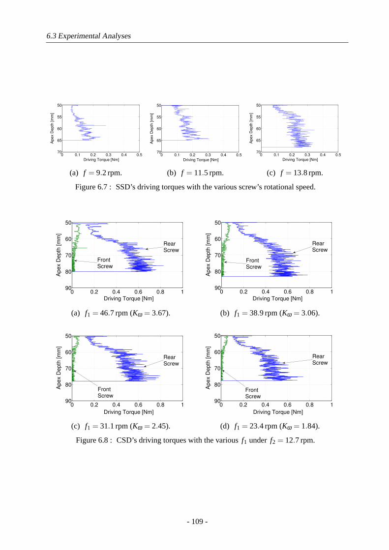
6.3 Experimental Analyses
0 0.1 0.2 0.3 0.4 0.5
50
55
60
65
70
Driving Torque [Nm]
Ap
ex D
ep
th [
mm
]
(a) f = 9.2rpm.
0 0.1 0.2 0.3 0.4 0.5
50
55
60
65
70
Driving Torque [Nm]
Ap
ex D
ep
th [
mm
]
(b) f = 11.5rpm.
0 0.1 0.2 0.3 0.4 0.5
50
55
60
65
70
Driving Torque [Nm]
Ap
ex D
ep
th [
mm
]
(c) f = 13.8rpm.
Figure 6.7 : SSD’s driving torques with the various screw’s rotational speed.
0 0.2 0.4 0.6 0.8 1
50
60
70
80
90
Driving Torque [Nm]
Ap
ex D
ep
th [
mm
]
Front
Screw
Rear
Screw
(a) f1 = 46.7rpm (Kω = 3.67).
0 0.2 0.4 0.6 0.8 1
50
60
70
80
90
Driving Torque [Nm]
Ap
ex D
ep
th [
mm
]
Front
Screw
Rear
Screw
(b) f1 = 38.9rpm (Kω = 3.06).
0 0.2 0.4 0.6 0.8 1
50
60
70
80
90
Driving Torque [Nm]
Ap
ex D
ep
th [
mm
]
Rear
Screw
Front
Screw
(c) f1 = 31.1rpm (Kω = 2.45).
0 0.2 0.4 0.6 0.8 1
50
60
70
80
90
Driving Torque [Nm]
Ap
ex D
ep
th [
mm
]
Front
Screw
Rear
Screw
(d) f1 = 23.4rpm (Kω = 1.84).
Figure 6.8 : CSD’s driving torques with the variousf1 under f2 = 12.7rpm.
- 109 -
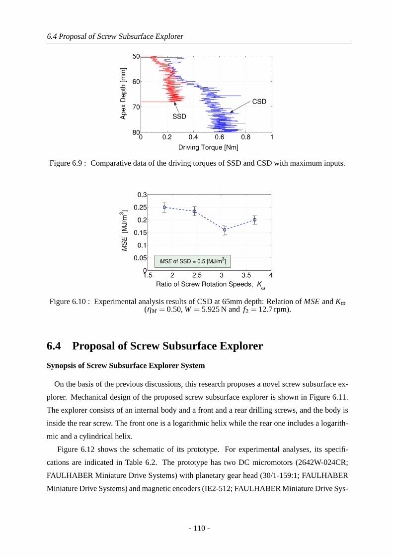
6.4 Proposal of Screw Subsurface Explorer
0 0.2 0.4 0.6 0.8 1
50
60
70
80
Driving Torque [Nm]
Ap
ex D
ep
th [
mm
]
CSD
SSD
Figure 6.9 : Comparative data of the driving torques of SSD and CSD with maximum inputs.
1.5 2 2.5 3 3.5 40
0.05
0.1
0.15
0.2
0.25
0.3
Ratio of Screw Rotation Speeds, Kω
MS
E
[MJ/m
3]
MSE of SSD = 0.5 [MJ/m3]
Figure 6.10 : Experimental analysis results of CSD at 65mm depth: Relation ofMSEandKω(ηM = 0.50, W = 5.925N and f2 = 12.7rpm).
6.4 Proposal of Screw Subsurface Explorer
Synopsis of Screw Subsurface Explorer System
On the basis of the previous discussions, this research proposes a novel screw subsurface ex-
plorer. Mechanical design of the proposed screw subsurface explorer is shown in Figure 6.11.
The explorer consists of an internal body and a front and a rear drilling screws, and the body is
inside the rear screw. The front one is a logarithmic helix while the rear one includes a logarith-
mic and a cylindrical helix.
Figure 6.12 shows the schematic of its prototype. For experimental analyses, its specifi-
cations are indicated in Table 6.2. The prototype has two DC micromotors (2642W-024CR;
FAULHABER Miniature Drive Systems) with planetary gear head (30/1-159:1; FAULHABER
Miniature Drive Systems) and magnetic encoders (IE2-512; FAULHABER Miniature Drive Sys-
- 110 -
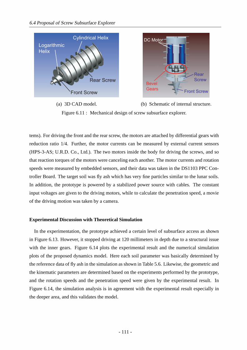
6.4 Proposal of Screw Subsurface Explorer
Logarithmic
Helix
Cylindrical Helix
Rear Screw
Front Screw
(a) 3D CAD model.
DC Motor
Bevel
GearsFront Screw
Rear
Screw
(b) Schematic of internal structure.
Figure 6.11 : Mechanical design of screw subsurface explorer.
tems). For driving the front and the rear screw, the motors are attached by differential gears with
reduction ratio 1/4. Further, the motor currents can be measured by external current sensors
(HPS-3-AS; U.R.D. Co., Ltd.). The two motors inside the body for driving the screws, and so
that reaction torques of the motors were canceling each another. The motor currents and rotation
speeds were measured by embedded sensors, and their data was taken in the DS1103 PPC Con-
troller Board. The target soil was fly ash which has very fine particles similar to the lunar soils.
In addition, the prototype is powered by a stabilized power source with cables. The constant
input voltages are given to the driving motors, while to calculate the penetration speed, a movie
of the driving motion was taken by a camera.
Experimental Discussion with Theoretical Simulation
In the experimentation, the prototype achieved a certain level of subsurface access as shown
in Figure 6.13. However, it stopped driving at 120 millimeters in depth due to a structural issue
with the inner gears. Figure 6.14 plots the experimental result and the numerical simulation
plots of the proposed dynamics model. Here each soil parameter was basically determined by
the reference data of fly ash in the simulation as shown in Table 5.6. Likewise, the geometric and
the kinematic parameters are determined based on the experiments performed by the prototype,
and the rotation speeds and the penetration speed were given by the experimental result. In
Figure 6.14, the simulation analysis is in agreement with the experimental result especially in
the deeper area, and this validates the model.
- 111 -
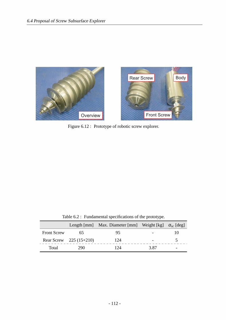
6.4 Proposal of Screw Subsurface Explorer
Overview
Rear Screw Body
Front Screw
Figure 6.12 : Prototype of robotic screw explorer.
Table 6.2 : Fundamental specifications of the prototype.
Length [mm] Max. Diameter [mm] Weight [kg] αsc [deg]
Front Screw 65 95 - 10
Rear Screw 225 (15+210) 124 - 5
Total 290 124 3.87 -
- 112 -
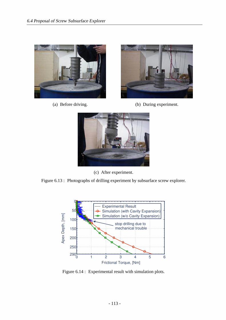
6.4 Proposal of Screw Subsurface Explorer
(a) Before driving. (b) During experiment.
(c) After experiment.
Figure 6.13 : Photographs of drilling experiment by subsurface screw explorer.
0 1 2 3 4 5 6
0
50
100
150
200
250
290
Frictional Torque, [Nm]
Ap
ex D
ep
th,
[mm
]
Experimental Result
Simulation (with Cavity Expansion)
Simulation (w/o Cavity Expansion)
stop drilling due to
mechanical trouble
Figure 6.14 : Experimental result with simulation plots.
- 113 -
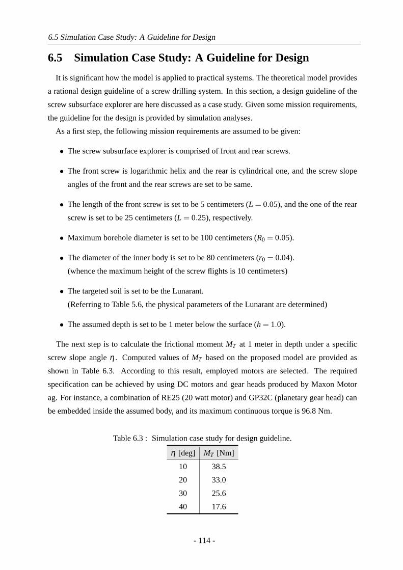
6.5 Simulation Case Study: A Guideline for Design
6.5 Simulation Case Study: A Guideline for Design
It is significant how the model is applied to practical systems. The theoretical model provides
a rational design guideline of a screw drilling system. In this section, a design guideline of the
screw subsurface explorer are here discussed as a case study. Given some mission requirements,
the guideline for the design is provided by simulation analyses.
As a first step, the following mission requirements are assumed to be given:
• The screw subsurface explorer is comprised of front and rear screws.
• The front screw is logarithmic helix and the rear is cylindrical one, and the screw slope
angles of the front and the rear screws are set to be same.
• The length of the front screw is set to be 5 centimeters (L = 0.05), and the one of the rear
screw is set to be 25 centimeters (L = 0.25), respectively.
• Maximum borehole diameter is set to be 100 centimeters (R0 = 0.05).
• The diameter of the inner body is set to be 80 centimeters (r0 = 0.04).
(whence the maximum height of the screw flights is 10 centimeters)
• The targeted soil is set to be the Lunarant.
(Referring to Table 5.6, the physical parameters of the Lunarant are determined)
• The assumed depth is set to be 1 meter below the surface (h = 1.0).
The next step is to calculate the frictional momentMT at 1 meter in depth under a specific
screw slope angleη . Computed values ofMT based on the proposed model are provided as
shown in Table 6.3. According to this result, employed motors are selected. The required
specification can be achieved by using DC motors and gear heads produced by Maxon Motor
ag. For instance, a combination of RE25 (20 watt motor) and GP32C (planetary gear head) can
be embedded inside the assumed body, and its maximum continuous torque is 96.8 Nm.
Table 6.3 : Simulation case study for design guideline.
η [deg] MT [Nm]
10 38.5
20 33.0
30 25.6
40 17.6
- 114 -
6.6 Summary
6.6 Summary
In the summary of these experimental analyses, the above results elaborate on the underlying
properties of the CSD under various screw driving modes. Through the experimental analyses,
the following remarks regarding the proposed screw drilling mechanism, CSD, are especially
concluded as key notes:
• Penetration speed was be attributed to rotational speed and input power.
• Penetration speed depended greatly on the driving property of the rear screw.
(because making a borehole for advancing is governed by the rear screw driving)
• The non-reaction condition was able to be achieved by two motors.
(realization of efficient drilling)
• Appropriate drilling condition: Neighborhood ofKω = 2 for quartz sand andKω = 3 for
the Lunarant (lunar soil simulant).
(it might be constrained by the relative ratio of the screw geometry and soil properties
and the reason for the incidence of a constant appropriate condition is estimated to be the
influence by transferring soil from the front screw to the rear one)
Furthermore, this research proposed and developed the screw subsurface explorer. The ex-
perimentation of the prototyped robot was carried out, and its result was discussed with the
comparative analysis of the numerical simulation. Mechanical issues should be addressed in
future works in order for the prototype to conduct more challenging experiments in a deeper
subsurface. Model analysis in such conditions should also be conducted in order to enhance the
reliability of the robotic explorer. In addition, the effect of the contra-rotor mechanism and the
identification of indeterminate soil parameters need to be considered in the theoretical study.
This chapter also indicated the drilling experimental result of the screw subsurface explorer.
The result was discussed with the simulations. From this, it was confirmed that the proposed
model is feasible to estimate the frictional moment.
- 115 -

6.6 Summary
- 116 -
Chapter 7. Conclusions
7.1 Concluding Remarks
This research has addressed mainly the soil-screw interaction. This chapter summarizes this
dissertation and the main resulting conclusions are described as follows.
Chapter 2: Archimedean Screw Mechanism
Chapter 2 introduced the mathematical definitions of the fundamental screw helices, es-
pecially the screw’s geometric and kinematic parameters. Based upon the definitions,
arbitrary helical shapes of logarithmic and cylindrical screws can be expressed in math-
ematical form. Then, possible advantages of the screw mechanism for applying to the
surface and the subsurface locomotion were stated concisely. Additionally, Chapter 2
summarized related works of the screw applications, not only locomotion in soft terrain.
Chapter 3: Modeling of Screw Surface Locomotion
Chapter 3 elaborated the uncommon locomotion method using the Archimedean screw
mechanism. At first, this chapter discussed advantages of the screw mechanism by com-
parison of conventional locomotion gears such as a wheel and a track. The Archimedean
screw mechanism is expected to exert enough traction even it is buried into soil. Accord-
ingly, it is robust to getting stuck in the soil in addition to its structural simplicity. In this
dissertation, the Screw Dive Rover system driven by the Archimedean screw units was
proposed as a new-typed rover specialized for traveling on the soil. Then, this chapter
mainly addressed the soil-screw interaction modeling for the surface locomotion by the
Archimedean screw unit. Two types of the model concepts were here considered. One
was the interaction model based on the skin friction between the screw flights and the soil.
Another was the model based on the terramechanic studies, which are able to cover the
compression characteristics and the shear phenomena of soil. These models were evalu-
ated by the simulation analyses. The skin friction model was very simple and it enabled
- 117 -
7.1 Concluding Remarks
to easily control the movement. Its consistency with the empirical maneuvers, however,
was incompatible in practice. Meanwhile, although the terramechanics-based model in-
dicated preferable compatibility with the empirical maneuvers (as stated in Chapter 4), it
became complicated. In particular, the terramechanics model was able to indicate a simi-
lar tendency resulted in experimental results (Chapter 4). Based upon these remarks, the
new synthetic model was proposed by combining skin friction and terramechanics. The
synthetic model can demonstrate more practical interaction, and provided a significant
guideline for using the screw mechanism.
Chapter 4: Experimental Characteristics of Screw Surface Locomotion
Chapter 4 addressed the experimental analyses of the Archimedean screw unit for surface
locomotion. In this chapter the experimental trafficability of the single screw unit and
the experimental maneuverability of the Screw Drive Rover system were investigated by
the indoor experiments. The trafficability and the maneuverability suggested how the
interactive mechanics between the screw unit and the soil should work. Furthermore,
the trafficability was quantitatively discussed by comparing with the simulations of the
proposed model. From these analyses, the validity of the proposed model was indicated.
In the maneuverability and the trafficability tests, quantitative and qualitative analyses
were conducted. The experimental results also contributes to the interaction modeling
process in Chapter 3.
Chapter 5: Modeling and Analysis of Screw Subsurface Locomotion
Chapter 5 investigated subsurface locomotion by the Archimedean screw mechanism. To
advance in the soil, it was indicated for the subsurface explorer system to require an active
force by computational prediction. Also, the subsurface locomotion strategy was qual-
itatively defined based on the past literature [163]. Through the theoretical discussion
on feasibility analyses of the soil compaction for making a space, this research pointed
out the importance of removing fore-soil backward. According to these considerations,
effectiveness of the Archimedean screw was indicated. Following these remarks, this
chapter introduced the novel soil-screw interaction model of the subsurface locomotion in
the soil (drilling into the soil). The proposed model was analyzed by the parametric sim-
ulations, and then its characteristics were numerically examined. The model validation
was also evaluated by the experimental result and the numerical simulation. This chapter
- 118 -
7.2 Future Works
contributes to a novel concept of the soil-screw interaction for general applications of the
screw structure in the soft terrain.
Chapter 6: Proposal of Effective Screw Drilling Mechanism
Chapter 6 proposed a new effective screw drilling mechanism, called CSD (Contra-rotor
Screw Drilling) mechanism to achieve efficient screw drilling. This new mechanism aimed
to agitate compacted subsurface soil. Also, the CSD mechanism was able to cancel the
reaction torques of the two motors embedded in the body. This disabled the reacting body
rotation, and normal screw rotations and self-propulsion could thus be achieved without
any ground bases. The CSD was experimentally analyzed by usingSEandMSE indexes.
From the experimental analyses, it was confirmed that the CSD has the proper condition
when the front screw’s rotational speed is 2∼3 times greater than the rear one. Although
the condition depends on soil types and the screw geometry, it is an interesting remark that
a certain optimal condition exists. In addition, in this chapter a new subsurface explorer
by using the Archimedean screw mechanism was proposed. The proposed explorer was
designed to burrow into the soil by itself. The drilling experiment of the explorer was
carried out, and then its result was examined by comparison with the developed model in
the Chapter 5. From the experimentation, it was confirmed that the theoretical estimate
moderately meets the experimental result. Finally, the simulation case study of the screw’s
design guideline was exampled.
7.2 Future Works
This research has several future works to be addressed.
With regard to the surface locomotion by the screw, the interaction model needs to newly
consider boundary conditions at the ends of the screw units. Further to this, the model does
not include an inclination of the screw units to terrain surface. Thus, as a future work, the
model should be improved in order to discuss not only its stationary motion, but its dynamic
motion. Also, A quantitative evaluation of the maneuverability remains to be an undiscussed
subject. Practically, terrain conditions should be accurately controlled in order to validate quan-
titative maneuvers. In another viewpoint, path-following control will be needed to apply the
Archimedean screw mechanism to exploration rovers. As mentioned before, the precise mod-
eling of the soil-screw interaction is quite difficult due to terrain uncertainty or irregularity.
Therefore, a qualitative control will be achieved but a quantitative control will not be realized
- 119 -
7.2 Future Works
by just feedback control technique based on internal sensors. In practical rover missions, visual
tracking or landmark tracking by cameras is a prospective approach. To follow the given path,
autonomous/semi-autonomous trajectory modification must be conducted by sequential compu-
tation of error distance from desired path. By using the feedback control with visual information,
the locomotion control will be achieved even in unknown surfaces. The establishment of such
control scheme is one of the possible directions.
As for the subsurface locomotion by the screw, identifications of some soil parameters of the
proposed model need to be examined, especially at deeper areas in soil layer. Actually, de-
termination of the parameter ranges is enough for evaluating the model at the deep areas. In
particular, it is only necessary to deal with the most stringent condition for drilling into the com-
pacted regolith. As a result, selections of the most stringent parameters will be next challenges.
To quantitatively evaluate details of the proposed models, each element in the models will be
required to be measured by various sensors. Further to these future works, generalized concept
of the proposed contra-rotor screw mechanism must be established to broaden the range of its
application.
On the other hand, effects of gravity and vacuum environments are additional challenges to
be addressed for both the surface and the subsurface locomotion. In fact, gravitational changes
and vacuum levels will affect screw’s performances. Enhancement of feasibility and reliability
of the screw mechanism in harsh space environment should be ensured and is an important task
to be discussed.
- 120 -
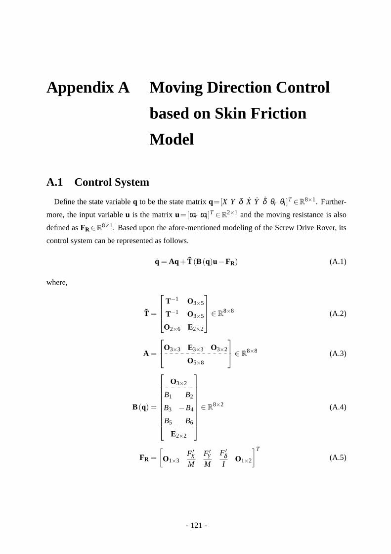
Appendix A Moving Direction Control
based on Skin Friction
Model
A.1 Control System
Define the state variableq to be the state matrixq=[X Y δ X Y δ θr θl ]T ∈R8×1. Further-
more, the input variableu is the matrixu=[ωr ωl ]T ∈R2×1 and the moving resistance is also
defined asFR∈R8×1. Based upon the afore-mentioned modeling of the Screw Drive Rover, its
control system can be represented as follows.
q = Aq + T (B(q)u−FR) (A.1)
where,
T =
T−1 O3×5
T−1 O3×5
O2×6 E2×2
∈ R8×8 (A.2)
A =
O3×3 E3×3 O3×2
O5×8
∈ R8×8 (A.3)
B(q) =
O3×2
B1 B2
B3 −B4
B5 B6
E2×2
∈ R8×2 (A.4)
FR =[O1×3
F ′XM
F ′YM
F ′δI
O1×2
]T
(A.5)
- 121 -
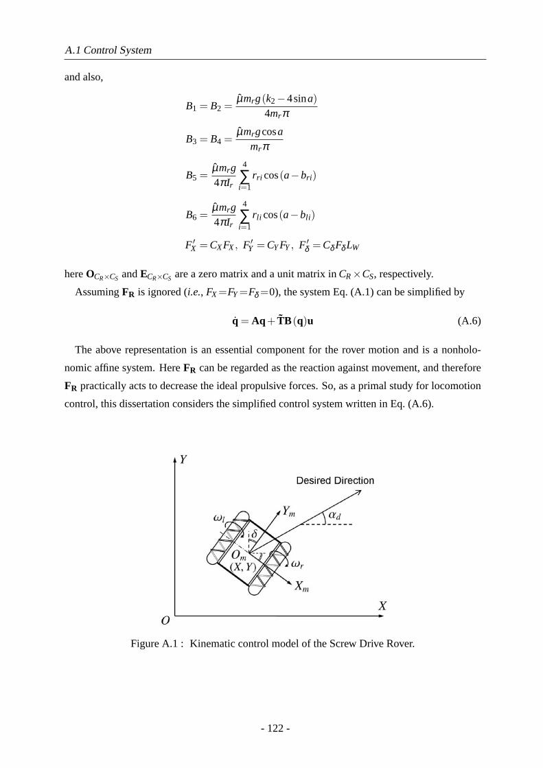
A.1 Control System
and also,
B1 = B2 =µmrg(k2−4sina)
4mrπ
B3 = B4 =µmrgcosa
mrπ
B5 =µmrg4πIr
4
∑i=1
rri cos(a−bri )
B6 =µmrg4πIr
4
∑i=1
r li cos(a−bli )
F ′X = CXFX, F ′Y = CYFY, F ′δ = Cδ Fδ LW
hereOCR×CS andECR×CS are a zero matrix and a unit matrix inCR×CS, respectively.
AssumingFR is ignored (i.e., FX=FY=Fδ =0), the system Eq. (A.1) can be simplified by
q = Aq + TB (q)u (A.6)
The above representation is an essential component for the rover motion and is a nonholo-
nomic affine system. HereFR can be regarded as the reaction against movement, and therefore
FR practically acts to decrease the ideal propulsive forces. So, as a primal study for locomotion
control, this dissertation considers the simplified control system written in Eq. (A.6).
Figure A.1 : Kinematic control model of the Screw Drive Rover.
- 122 -
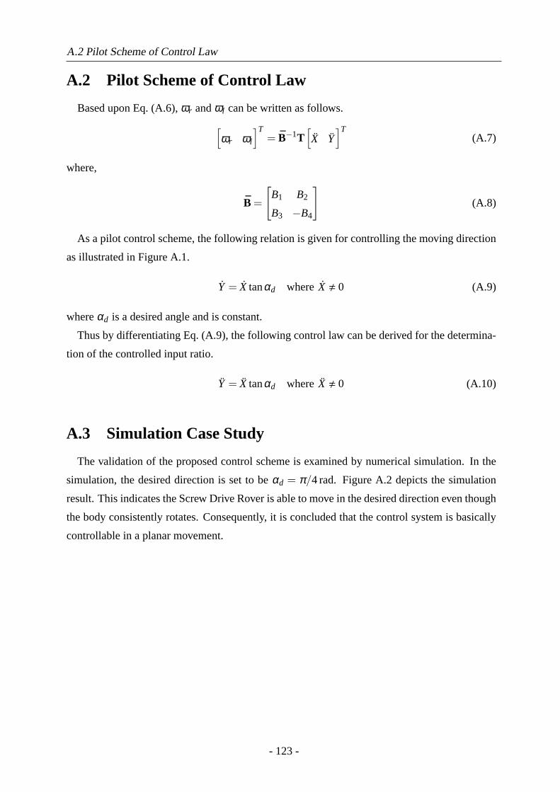
A.2 Pilot Scheme of Control Law
A.2 Pilot Scheme of Control Law
Based upon Eq. (A.6),ωr andωl can be written as follows.
[ωr ωl
]T= B−1T
[X Y
]T(A.7)
where,
B =
[B1 B2
B3 −B4
](A.8)
As a pilot control scheme, the following relation is given for controlling the moving direction
as illustrated in Figure A.1.
Y = X tanαd whereX , 0 (A.9)
whereαd is a desired angle and is constant.
Thus by differentiating Eq. (A.9), the following control law can be derived for the determina-
tion of the controlled input ratio.
Y = X tanαd whereX , 0 (A.10)
A.3 Simulation Case Study
The validation of the proposed control scheme is examined by numerical simulation. In the
simulation, the desired direction is set to beαd = π/4rad. Figure A.2 depicts the simulation
result. This indicates the Screw Drive Rover is able to move in the desired direction even though
the body consistently rotates. Consequently, it is concluded that the control system is basically
controllable in a planar movement.
- 123 -
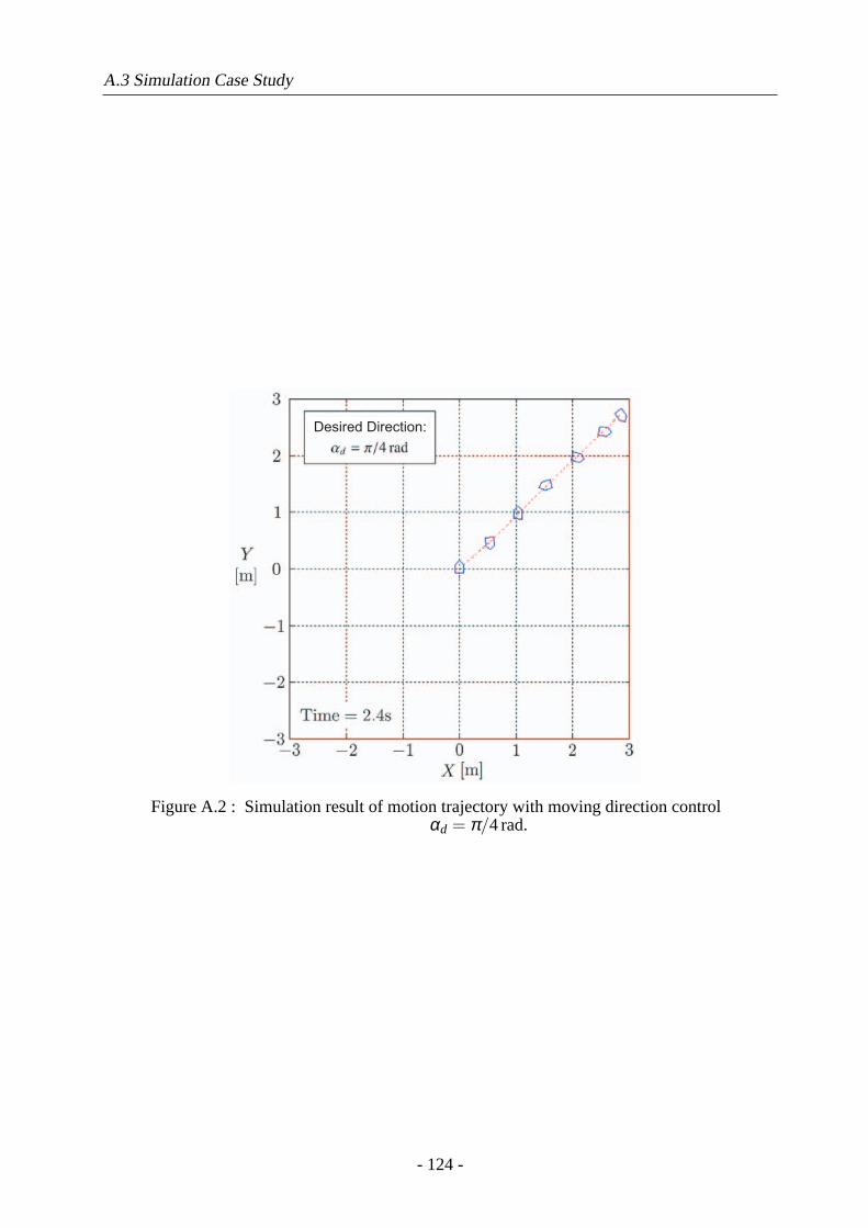
A.3 Simulation Case Study
Desired Direction:
Figure A.2 : Simulation result of motion trajectory with moving direction controlαd = π/4rad.
- 124 -
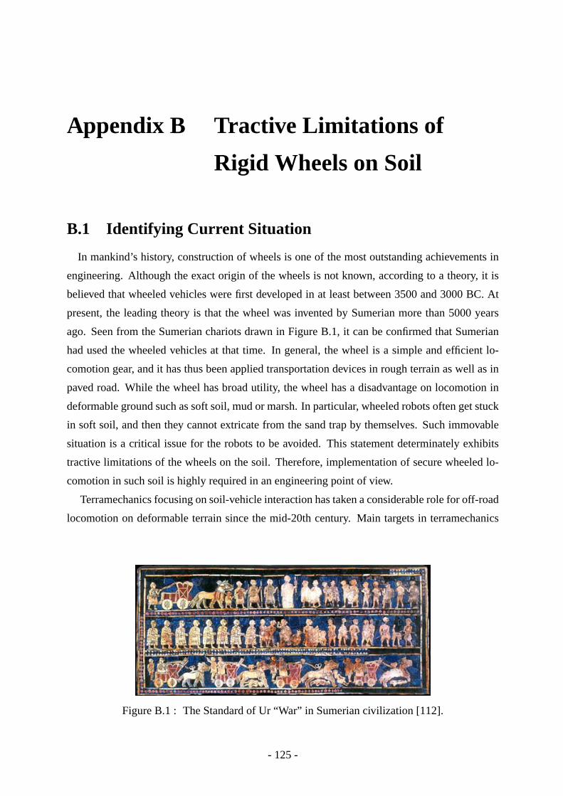
Appendix B Tractive Limitations of
Rigid Wheels on Soil
B.1 Identifying Current Situation
In mankind’s history, construction of wheels is one of the most outstanding achievements in
engineering. Although the exact origin of the wheels is not known, according to a theory, it is
believed that wheeled vehicles were first developed in at least between 3500 and 3000 BC. At
present, the leading theory is that the wheel was invented by Sumerian more than 5000 years
ago. Seen from the Sumerian chariots drawn in Figure B.1, it can be confirmed that Sumerian
had used the wheeled vehicles at that time. In general, the wheel is a simple and efficient lo-
comotion gear, and it has thus been applied transportation devices in rough terrain as well as in
paved road. While the wheel has broad utility, the wheel has a disadvantage on locomotion in
deformable ground such as soft soil, mud or marsh. In particular, wheeled robots often get stuck
in soft soil, and then they cannot extricate from the sand trap by themselves. Such immovable
situation is a critical issue for the robots to be avoided. This statement determinately exhibits
tractive limitations of the wheels on the soil. Therefore, implementation of secure wheeled lo-
comotion in such soil is highly required in an engineering point of view.
Terramechanics focusing on soil-vehicle interaction has taken a considerable role for off-road
locomotion on deformable terrain since the mid-20th century. Main targets in terramechanics
Figure B.1 : The Standard of Ur “War” in Sumerian civilization [112].
- 125 -
B.2 Terramechanics Model of a Rigid Wheel
are basically machines for transportation, agriculture or extraterrestrial investigation. Accumu-
lated findings in terramechanics can provide practical guidelines when discussing locomotion
on soft soil such as lunar or martian soil. One of the mainstream approaches in terramechanics
is the study on semi-empirical models regarding steady states of wheels and tracks on natural
terrain (e.g. [66,73,75,82,83]). Furthermore, in recent years soil parameter estimation has been
also studied from a geological standpoint [84, 89, 95]. Likewise, visual sinkage measurement
by a camera [88] or online slip prediction method by motor current [87] has been currently
addressed. As technical applications, some have studied slope climbing [86], steering charac-
teristics [72,76,90] and slope traversability [94]. Most of them have been commonly discussed
based upon the conventional models.
Although the above expansion has been accomplished until now, the tractive limitations of the
wheel on the soil is less well understood. The tractive limitations denote an unmovable and a
critical state with much slippage, and it should be thus avoided for a mobile robot. Getting stuck
in the soil should be avoided for the robots as mentioned previously, and then discussion of the
limitations is expected to lead to a solution for that. So this appendix indicates the tractive limita-
tions by using the terramechanics models in an attempt to answer the question “What parameter
is a key factor to avoid getting stuck into the soft soil?”. In addition to this, an application
methodology of the models is also discussed with conventional experimental approaches.
B.2 Terramechanics Model of a Rigid Wheel
Terramechanics contributes to formulate the soil-wheel interaction, including semi-empirical
factors. The basic formulae express just static and convergent states, and are generally derived
as follows [82].
DPw = rwbw
∫ θw f
θwr
(τ cosθw−σ sinθw)dθw (B.1)
Fz = rwbw
∫ θw f
θwr
(τ sinθw +σ cosθw)dθw (B.2)
Tw = r2wbw
∫ θw f
θwr
τ dθw (B.3)
whererw is wheel radius,bw is wheel width,θw is wheel angle,θw f is entry angle,θwr is exit
angle, andσ andτ are normal and shear stress of soil, respectively. The wheel is assumed not
to deploy any lugs or fins on its surface. These equations calculate drawbar pullDPw, vertical
force Fz and required torqueTw, and are principle parameters of wheel motion. In particular,
force equilibrium ofFz and wheel loadW must be satisfied.
- 126 -
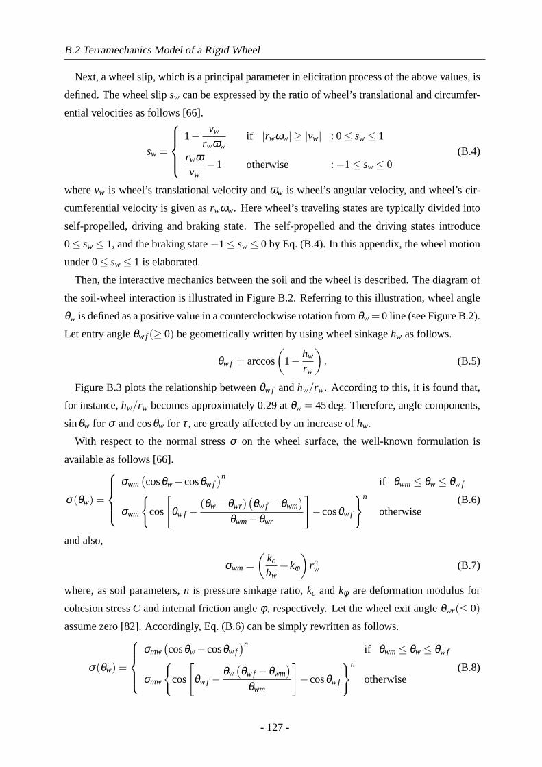
B.2 Terramechanics Model of a Rigid Wheel
Next, a wheel slip, which is a principal parameter in elicitation process of the above values, is
defined. The wheel slipsw can be expressed by the ratio of wheel’s translational and circumfer-
ential velocities as follows [66].
sw =
1− vw
rwωwif |rwωw| ≥ |vw| : 0≤ sw≤ 1
rwωvw
−1 otherwise :−1≤ sw≤ 0(B.4)
wherevw is wheel’s translational velocity andωw is wheel’s angular velocity, and wheel’s cir-
cumferential velocity is given asrwωw. Here wheel’s traveling states are typically divided into
self-propelled, driving and braking state. The self-propelled and the driving states introduce
0≤ sw≤ 1, and the braking state−1≤ sw≤ 0 by Eq. (B.4). In this appendix, the wheel motion
under0≤ sw≤ 1 is elaborated.
Then, the interactive mechanics between the soil and the wheel is described. The diagram of
the soil-wheel interaction is illustrated in Figure B.2. Referring to this illustration, wheel angle
θw is defined as a positive value in a counterclockwise rotation fromθw = 0 line (see Figure B.2).
Let entry angleθw f(≥ 0) be geometrically written by using wheel sinkagehw as follows.
θw f = arccos
(1− hw
rw
). (B.5)
Figure B.3 plots the relationship betweenθw f andhw/rw. According to this, it is found that,
for instance,hw/rw becomes approximately0.29 at θw = 45deg. Therefore, angle components,
sinθw for σ andcosθw for τ, are greatly affected by an increase ofhw.
With respect to the normal stressσ on the wheel surface, the well-known formulation is
available as follows [66].
σ(θw) =
σwm(cosθw−cosθw f
)nif θwm≤ θw≤ θw f
σwm
{cos
[θw f −
(θw−θwr)(θw f −θwm
)
θwm−θwr
]−cosθw f
}n
otherwise(B.6)
and also,
σwm =(
kc
bw+kφ
)rnw (B.7)
where, as soil parameters,n is pressure sinkage ratio,kc andkφ are deformation modulus for
cohesion stressC and internal friction angleφ , respectively. Let the wheel exit angleθwr(≤ 0)
assume zero [82]. Accordingly, Eq. (B.6) can be simply rewritten as follows.
σ(θw) =
σmw(cosθw−cosθw f
)nif θwm≤ θw≤ θw f
σmw
{cos
[θw f −
θw(θw f −θwm
)
θwm
]−cosθw f
}n
otherwise(B.8)
- 127 -
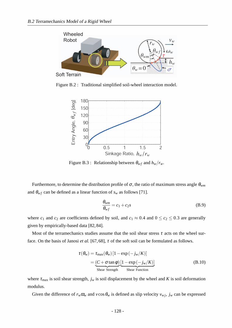
B.2 Terramechanics Model of a Rigid Wheel
Wheeled
Robot
Soft Terrain
Figure B.2 : Traditional simplified soil-wheel interaction model.
0 0.5 1 1.5 20
30
60
90
120
150
180
Sinkage Ratio,
En
try
An
gle
,
[de
g]
Figure B.3 : Relationship betweenθw f andhw/rw.
Furthermore, to determine the distribution profile ofσ , the ratio of maximum stress angleθwm
andθw f can be defined as a linear function ofsw as follows [71].
θwm
θw f= c1 +c2s (B.9)
wherec1 andc2 are coefficients defined by soil, andc1 ≈ 0.4 and0≤ c2 ≤ 0.3 are generally
given by empirically-based data [82,84].
Most of the terramechanics studies assume that the soil shear stressτ acts on the wheel sur-
face. On the basis of Janosiet al. [67,68],τ of the soft soil can be formulated as follows.
τ(θw) = τmax(θw) [1−exp(− jw/K)]
= (C+σ tanφ)︸ ︷︷ ︸Shear Strength
[1−exp(− jw/K)]︸ ︷︷ ︸Shear Function
(B.10)
whereτmax is soil shear strength,jw is soil displacement by the wheel andK is soil deformation
modulus.
Given the difference ofrwωw andvcosθw is defined as slip velocityvw j, jw can be expressed
- 128 -
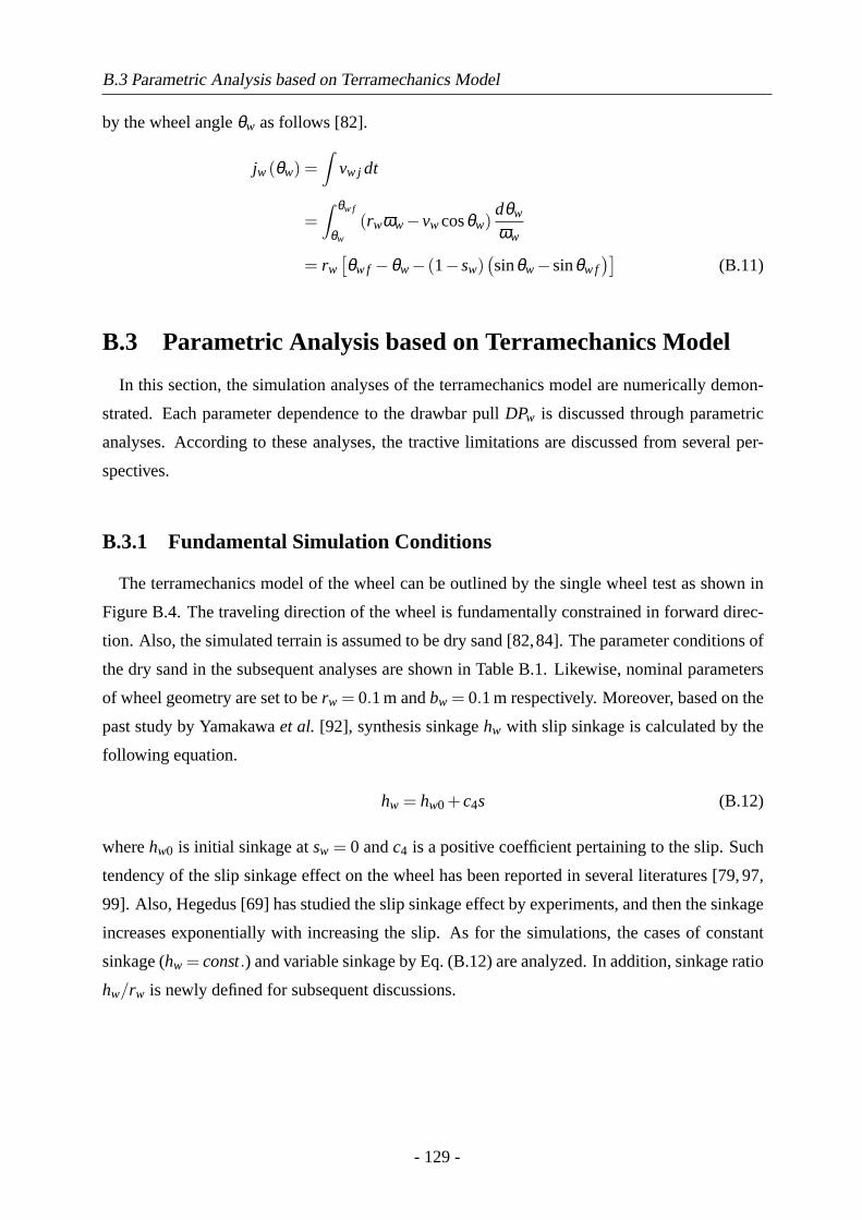
B.3 Parametric Analysis based on Terramechanics Model
by the wheel angleθw as follows [82].
jw(θw) =∫
vw j dt
=∫ θw f
θw
(rwωw−vwcosθw)dθw
ωw
= rw[θw f −θw− (1−sw)
(sinθw−sinθw f
)](B.11)
B.3 Parametric Analysis based on Terramechanics Model
In this section, the simulation analyses of the terramechanics model are numerically demon-
strated. Each parameter dependence to the drawbar pullDPw is discussed through parametric
analyses. According to these analyses, the tractive limitations are discussed from several per-
spectives.
B.3.1 Fundamental Simulation Conditions
The terramechanics model of the wheel can be outlined by the single wheel test as shown in
Figure B.4. The traveling direction of the wheel is fundamentally constrained in forward direc-
tion. Also, the simulated terrain is assumed to be dry sand [82,84]. The parameter conditions of
the dry sand in the subsequent analyses are shown in Table B.1. Likewise, nominal parameters
of wheel geometry are set to berw = 0.1m andbw = 0.1m respectively. Moreover, based on the
past study by Yamakawaet al. [92], synthesis sinkagehw with slip sinkage is calculated by the
following equation.
hw = hw0 +c4s (B.12)
wherehw0 is initial sinkage atsw = 0 andc4 is a positive coefficient pertaining to the slip. Such
tendency of the slip sinkage effect on the wheel has been reported in several literatures [79, 97,
99]. Also, Hegedus [69] has studied the slip sinkage effect by experiments, and then the sinkage
increases exponentially with increasing the slip. As for the simulations, the cases of constant
sinkage (hw = const.) and variable sinkage by Eq. (B.12) are analyzed. In addition, sinkage ratio
hw/rw is newly defined for subsequent discussions.
- 129 -
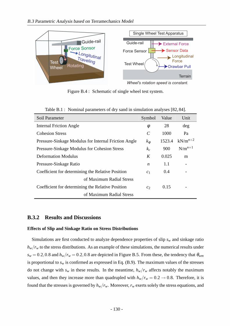
B.3 Parametric Analysis based on Terramechanics Model
Longitutinal TravelingRotating
Guide-rail
Force Sonsor
Test
Wheel
Wheel's rotation speed is constant.
Single Wheel Test Apparatus
Guide-rail
Force Sensor
Test Wheel
Terrain
Sensor Data
External Force
Drawbar Pull
Longitudinal
Force
Figure B.4 : Schematic of single wheel test system.
Table B.1 : Nominal parameters of dry sand in simulation analyses [82,84].
Soil Parameter Symbol Value Unit
Internal Friction Angle φ 28 deg
Cohesion Stress C 1000 Pa
Pressure-Sinkage Modulus for Internal Friction Angle kφ 1523.4 kN/mn+2
Pressure-Sinkage Modulus for Cohesion Stress kc 900 N/mn+1
Deformation Modulus K 0.025 m
Pressure-Sinkage Ratio n 1.1 -
Coefficient for determining the Relative Position c1 0.4 -
of Maximum Radial Stress
Coefficient for determining the Relative Position c2 0.15 -
of Maximum Radial Stress
B.3.2 Results and Discussions
Effects of Slip and Sinkage Ratio on Stress Distributions
Simulations are first conducted to analyze dependence properties of slipsw and sinkage ratio
hw/rw to the stress distributions. As an example of these simulations, the numerical results under
sw = 0.2,0.8 andhw/rw = 0.2,0.8 are depicted in Figure B.5. From these, the tendency thatθwm
is proportional tosw is confirmed as expressed in Eq. (B.9). The maximum values of the stresses
do not change withsw in these results. In the meantime,hw/rw affects notably the maximum
values, and then they increase more than quadrupled withhw/rw = 0.2→ 0.8. Therefore, it is
found that the stresses is governed byhw/rw. Moreover,rw exerts solely the stress equations, and
- 130 -
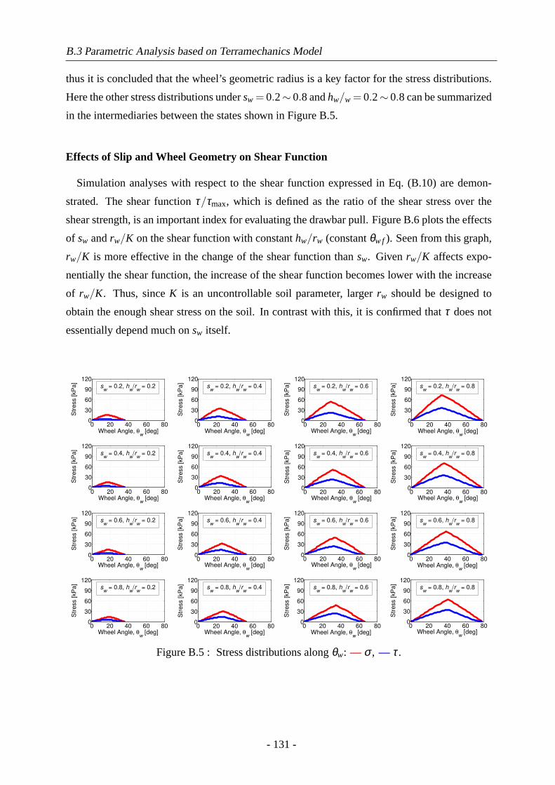
B.3 Parametric Analysis based on Terramechanics Model
thus it is concluded that the wheel’s geometric radius is a key factor for the stress distributions.
Here the other stress distributions undersw = 0.2∼ 0.8 andhw/w = 0.2∼ 0.8 can be summarized
in the intermediaries between the states shown in Figure B.5.
Effects of Slip and Wheel Geometry on Shear Function
Simulation analyses with respect to the shear function expressed in Eq. (B.10) are demon-
strated. The shear functionτ/τmax, which is defined as the ratio of the shear stress over the
shear strength, is an important index for evaluating the drawbar pull. Figure B.6 plots the effects
of sw andrw/K on the shear function with constanthw/rw (constantθw f ). Seen from this graph,
rw/K is more effective in the change of the shear function thansw. Given rw/K affects expo-
nentially the shear function, the increase of the shear function becomes lower with the increase
of rw/K. Thus, sinceK is an uncontrollable soil parameter, largerrw should be designed to
obtain the enough shear stress on the soil. In contrast with this, it is confirmed thatτ does not
essentially depend much onsw itself.
0 20 40 60 800
30
60
90
120
Wheel Angle, θw
[deg]
Str
ess [kP
a]
sw
= 0.2, hw
/rw
= 0.2
0 20 40 60 800
30
60
90
120
Str
ess [kP
a]
Wheel Angle, θw
[deg]
sw
= 0.2, hw
/rw
= 0.4
0 20 40 60 800
30
60
90
120
Wheel Angle, θw
[deg]
Str
ess [kP
a]
sw
= 0.2, hw
/rw
= 0.6
0 20 40 60 800
30
60
90
120
Wheel Angle, θw
[deg]
Str
ess [kP
a]
sw
= 0.2, hw
/rw
= 0.8
0 20 40 60 800
30
60
90
120
Wheel Angle, θw
[deg]
Str
ess [kP
a]
sw
= 0.4, hw
/rw
= 0.2
0 20 40 60 800
30
60
90
120
Wheel Angle, θw
[deg]
Str
ess [kP
a]
sw
= 0.4, hw
/rw
= 0.4
0 20 40 60 800
30
60
90
120
Wheel Angle, θw
[deg]
Str
ess [kP
a]
sw
= 0.4, hw
/rw
= 0.6
0 20 40 60 800
30
60
90
120
Wheel Angle, θw
[deg]
Str
ess [kP
a]
sw
= 0.4, hw
/rw
= 0.8
0 20 40 60 800
30
60
90
120
Wheel Angle, θw
[deg]
Str
ess [kP
a]
sw
= 0.6, hw
/rw
= 0.2
0 20 40 60 800
30
60
90
120
Wheel Angle, θw
[deg]
Str
ess [kP
a]
sw
= 0.6, hw
/rw
= 0.4
0 20 40 60 800
30
60
90
120
Wheel Angle, θw
[deg]
Str
ess [kP
a]
sw
= 0.6, hw
/rw
= 0.6
0 20 40 60 800
30
60
90
120
Wheel Angle, θw
[deg]
Str
ess [kP
a]
sw
= 0.6, hw
/rw
= 0.8
0 20 40 60 800
30
60
90
120
Wheel Angle, θw
[deg]
Str
ess [kP
a]
sw
= 0.8, hw
/rw
= 0.2
0 20 40 60 800
30
60
90
120
Wheel Angle, θw
[deg]
Str
ess [kP
a]
sw
= 0.8, hw
/rw
= 0.4
0 20 40 60 800
30
60
90
120
Wheel Angle, θw
[deg]
Str
ess [kP
a]
sw
= 0.8, hw
/rw
= 0.6
0 20 40 60 800
30
60
90
120
Wheel Angle, θw
[deg]
Str
ess [kP
a]
sw
= 0.8, hw
/rw
= 0.8
Figure B.5 : Stress distributions alongθw: — σ , — τ.
- 131 -
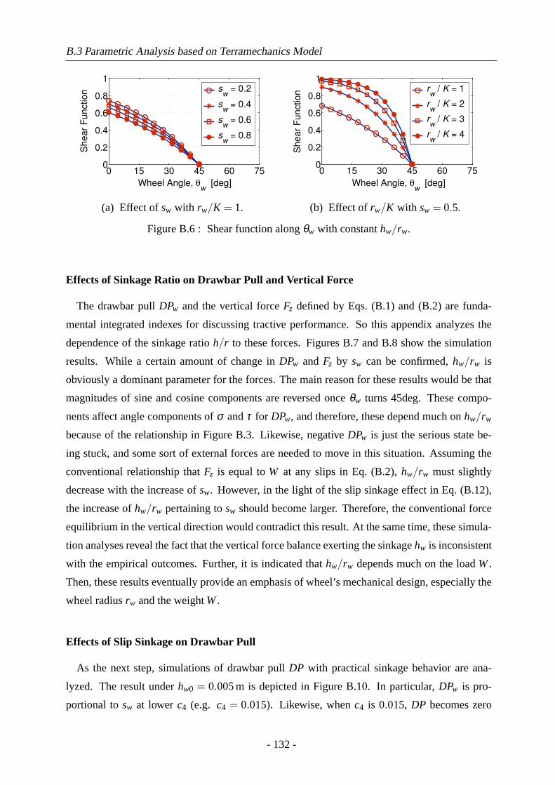
B.3 Parametric Analysis based on Terramechanics Model
0 15 30 45 60 750
0.2
0.4
0.6
0.8
1
Wheel Angle, θw
[deg]
Sh
ea
r F
un
ctio
n
sw
= 0.2
sw
= 0.4
sw
= 0.6
sw
= 0.8
(a) Effect ofsw with rw/K = 1.
0 15 30 45 60 750
0.2
0.4
0.6
0.8
1
Wheel Angle, θw
[deg]
Sh
ea
r F
un
ctio
n
rw
/ K = 1
rw
/ K = 2
rw
/ K = 3
rw
/ K = 4
(b) Effect ofrw/K with sw = 0.5.
Figure B.6 : Shear function alongθw with constanthw/rw.
Effects of Sinkage Ratio on Drawbar Pull and Vertical Force
The drawbar pullDPw and the vertical forceFz defined by Eqs. (B.1) and (B.2) are funda-
mental integrated indexes for discussing tractive performance. So this appendix analyzes the
dependence of the sinkage ratioh/r to these forces. Figures B.7 and B.8 show the simulation
results. While a certain amount of change inDPw and Fz by sw can be confirmed,hw/rw is
obviously a dominant parameter for the forces. The main reason for these results would be that
magnitudes of sine and cosine components are reversed onceθw turns45deg. These compo-
nents affect angle components ofσ andτ for DPw, and therefore, these depend much onhw/rw
because of the relationship in Figure B.3. Likewise, negativeDPw is just the serious state be-
ing stuck, and some sort of external forces are needed to move in this situation. Assuming the
conventional relationship thatFz is equal toW at any slips in Eq. (B.2),hw/rw must slightly
decrease with the increase ofsw. However, in the light of the slip sinkage effect in Eq. (B.12),
the increase ofhw/rw pertaining tosw should become larger. Therefore, the conventional force
equilibrium in the vertical direction would contradict this result. At the same time, these simula-
tion analyses reveal the fact that the vertical force balance exerting the sinkagehw is inconsistent
with the empirical outcomes. Further, it is indicated thathw/rw depends much on the loadW.
Then, these results eventually provide an emphasis of wheel’s mechanical design, especially the
wheel radiusrw and the weightW.
Effects of Slip Sinkage on Drawbar Pull
As the next step, simulations of drawbar pullDP with practical sinkage behavior are ana-
lyzed. The result underhw0 = 0.005m is depicted in Figure B.10. In particular,DPw is pro-
portional tosw at lowerc4 (e.g. c4 = 0.015). Likewise, whenc4 is 0.015, DP becomes zero
- 132 -
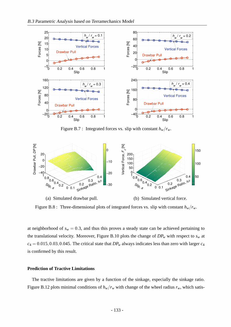
B.3 Parametric Analysis based on Terramechanics Model
0 0.2 0.4 0.6 0.8 1−5
0
5
10
15
20
25
Slip
Fo
rce
s [
N]
Drawbar Pull
Vertical Forces
hw
/ rw
= 0.1
0 0.2 0.4 0.6 0.8 1−20
0
20
40
60
80
Slip
Fo
rce
s [
N]
Drawbar Pull
Vertical Forces
hw
/ rw
= 0.2
0 0.2 0.4 0.6 0.8 1−20
0
40
80
120
160
Slip
Fo
rce
s [
N]
Drawbar Pull
Vertical Forces
hw
/ rw
= 0.3
0 0.2 0.4 0.6 0.8 1−40
0
80
160
240
Slip
Fo
rce
s [
N]
Vertical Forces
Drawbar Pull
hw
/ rw
= 0.4
Figure B.7 : Integrated forces vs. slip with constanthw/rw.
0.1
0.2
0.3
0.4
00.2
0.40.6
0.81
−40
−20
0
20
Sinkage Ratio
, h/r
Slip, s
Dra
wbar
Pull, D
P [N
]
−30
−20
−10
0
(a) Simulated drawbar pull.
0.1
0.2
0.3
0.4
00.2
0.40.6
0.810
50
100
150
200
Sinkage Ratio
, h/r
Slip, s
Vert
ical F
orc
e, F
z [N
]
50
100
150
(b) Simulated vertical force.
Figure B.8 : Three-dimensional plots of integrated forces vs. slip with constanthw/rw.
at neighborhood ofsw = 0.3, and thus this proves a steady state can be achieved pertaining to
the translational velocity. Moreover, Figure B.10 plots the change ofDPw with respect tosw at
c4 = 0.015,0.03,0.045. The critical state thatDPw always indicates less than zero with largerc4
is confirmed by this result.
Prediction of Tractive Limitations
The tractive limitations are given by a function of the sinkage, especially the sinkage ratio.
Figure B.12 plots minimal conditions ofhw/rw with change of the wheel radiusrw, which satis-
- 133 -
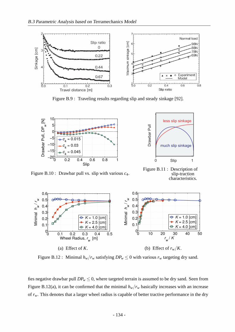
B.3 Parametric Analysis based on Terramechanics Model
Figure B.9 : Traveling results regarding slip and steady sinkage [92].
0 0.2 0.4 0.6 0.8 1−20
−15
−10
−5
0
5
10
Slip
Dra
wb
ar
Pu
ll, D
Pw
[N
]
c4 = 0.015
c4 = 0.03
c4 = 0.045
Figure B.10 : Drawbar pull vs. slip with variousc4.
Dra
wb
ar
Pu
ll
Slip 10
much slip sinkage
less slip sinkage
Figure B.11 : Description ofslip-traction
characteristics.
0 0.1 0.2 0.3 0.4 0.50
0.1
0.2
0.3
0.4
0.5
0.6
Wheel Radius, rw
[m]
Min
ima
l h
w /
rw
K = 1.0 [cm]
K = 2.5 [cm]
K = 4.0 [cm]
(a) Effect ofK.
0 10 20 30 40 500
0.1
0.2
0.3
0.4
0.5
0.6
rw
/ K
Min
ima
l h
w /
rw
K = 1.0 [cm]
K = 2.5 [cm]
K = 4.0 [cm]
(b) Effect ofrw/K.
Figure B.12 : Minimalhw/rw satisfyingDPw≤ 0 with variousrw targeting dry sand.
fies negative drawbar pullDPw≤ 0, where targeted terrain is assumed to be dry sand. Seen from
Figure B.12(a), it can be confirmed that the minimalhw/rw basically increases with an increase
of rw. This denotes that a larger wheel radius is capable of better tractive performance in the dry
- 134 -
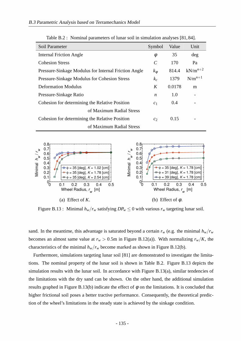
B.3 Parametric Analysis based on Terramechanics Model
Table B.2 : Nominal parameters of lunar soil in simulation analyses [81,84].
Soil Parameter Symbol Value Unit
Internal Friction Angle φ 35 deg
Cohesion Stress C 170 Pa
Pressure-Sinkage Modulus for Internal Friction Angle kφ 814.4 kN/mn+2
Pressure-Sinkage Modulus for Cohesion Stress kc 1379 N/mn+1
Deformation Modulus K 0.0178 m
Pressure-Sinkage Ratio n 1.0 -
Cohesion for determining the Relative Position c1 0.4 -
of Maximum Radial Stress
Cohesion for determining the Relative Position c2 0.15 -
of Maximum Radial Stress
0 0.1 0.2 0.3 0.4 0.50
0.1
0.2
0.3
0.4
0.5
0.6
0.7
0.8
Wheel Radius, rw
[m]
Min
ima
l h
w /
rw
φ = 35 [deg], K = 1.02 [cm]
φ = 35 [deg], K = 1.78 [cm]
φ = 35 [deg], K = 2.54 [cm]
(a) Effect ofK.
0 0.1 0.2 0.3 0.4 0.50
0.1
0.2
0.3
0.4
0.5
0.6
0.7
0.8
Wheel Radius, rw
[m]
Min
ima
l h
w /
rw
φ = 35 [deg], K = 1.78 [cm]
φ = 31 [deg], K = 1.78 [cm]
φ = 39 [deg], K = 1.78 [cm]
(b) Effect ofφ .
Figure B.13 : Minimalhw/rw satisfyingDPw≤ 0 with variousrw targeting lunar soil.
sand. In the meantime, this advantage is saturated beyond a certainrw (e.g. the minimalhw/rw
becomes an almost same value atrw > 0.5m in Figure B.12(a)). With normalizingrw/K, the
characteristics of the minimalhw/rw become marked as shown in Figure B.12(b).
Furthermore, simulations targeting lunar soil [81] are demonstrated to investigate the limita-
tions. The nominal property of the lunar soil is shown in Table B.2. Figure B.13 depicts the
simulation results with the lunar soil. In accordance with Figure B.13(a), similar tendencies of
the limitations with the dry sand can be shown. On the other hand, the additional simulation
results graphed in Figure B.13(b) indicate the effect ofφ on the limitations. It is concluded that
higher frictional soil poses a better tractive performance. Consequently, the theoretical predic-
tion of the wheel’s limitations in the steady state is achieved by the sinkage condition.
- 135 -
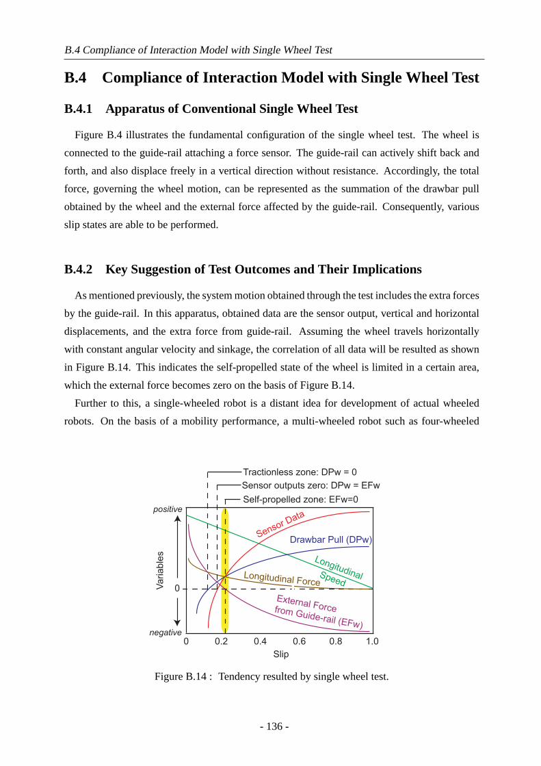
B.4 Compliance of Interaction Model with Single Wheel Test
B.4 Compliance of Interaction Model with Single Wheel Test
B.4.1 Apparatus of Conventional Single Wheel Test
Figure B.4 illustrates the fundamental configuration of the single wheel test. The wheel is
connected to the guide-rail attaching a force sensor. The guide-rail can actively shift back and
forth, and also displace freely in a vertical direction without resistance. Accordingly, the total
force, governing the wheel motion, can be represented as the summation of the drawbar pull
obtained by the wheel and the external force affected by the guide-rail. Consequently, various
slip states are able to be performed.
B.4.2 Key Suggestion of Test Outcomes and Their Implications
As mentioned previously, the system motion obtained through the test includes the extra forces
by the guide-rail. In this apparatus, obtained data are the sensor output, vertical and horizontal
displacements, and the extra force from guide-rail. Assuming the wheel travels horizontally
with constant angular velocity and sinkage, the correlation of all data will be resulted as shown
in Figure B.14. This indicates the self-propelled state of the wheel is limited in a certain area,
which the external force becomes zero on the basis of Figure B.14.
Further to this, a single-wheeled robot is a distant idea for development of actual wheeled
robots. On the basis of a mobility performance, a multi-wheeled robot such as four-wheeled
Sensor Data
Longitudinal
Slip
0 0.2 0.4 0.6 0.8 1.0
0Va
ria
ble
s
Drawbar Pull (DPw)
External Forcefrom Guide-rail (EFw)
positive
negative
Self-propelled zone: EFw=0
SpeedLongitudinal Force
Sensor outputs zero: DPw = EFw
Tractionless zone: DPw = 0
Figure B.14 : Tendency resulted by single wheel test.
- 136 -
B.5 Summary
or six-wheeled is practical configuration. Hence, most of the data acquired by the test simulate
the one wheel of the multi-wheeled robot with a difference between wheel motions. Given an
uncertainty by the dynamic behavior of the sinkage with slip change, what a positive traction
is able to be generated under lower slip and envisaged sinkage is important for the wheel’s
mechanical design.
B.5 Summary
This appendix theoretically investigates the tractive limitations of the wheeled robot in the
soil based on the conventional terramechanics models. Although all the analyses represent just
steady states, the static tractive limitations for the wheels can be newly indicated by evaluating
negative drawbar pull. In particular, it is found that the wheel radius and the weight become
important factors in order to avoid getting stuck in the soil. Also, the application methodology
of the terramechanic findings to the actual mobile robot is described by regarding as the one
wheel of the multi-wheeled robot. The subject of this appendix is providing an essential idea to
discuss wheeled robots in deformable terrain, and therefore, the results would contribute to the
development of such robot. Furthermore, as future works, traveling experiments of wheels are
necessary to evaluate and validate the theoretical predictions.
- 137 -

B.5 Summary
- 138 -
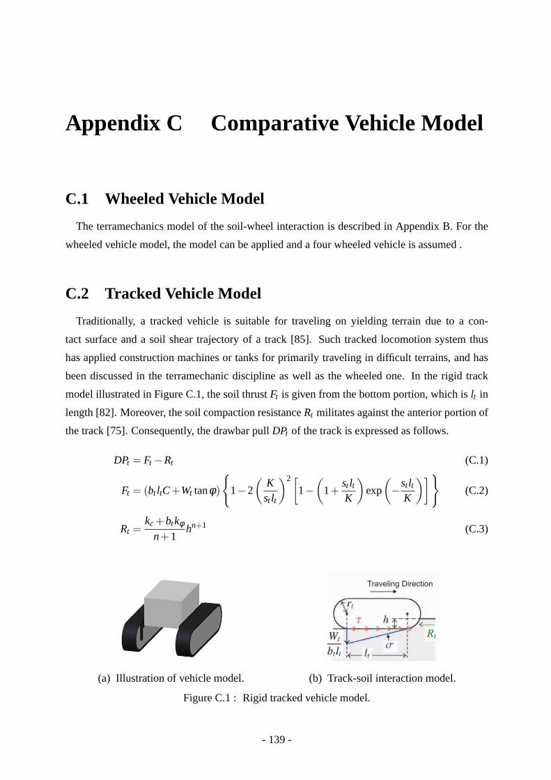
Appendix C Comparative Vehicle Model
C.1 Wheeled Vehicle Model
The terramechanics model of the soil-wheel interaction is described in Appendix B. For the
wheeled vehicle model, the model can be applied and a four wheeled vehicle is assumed .
C.2 Tracked Vehicle Model
Traditionally, a tracked vehicle is suitable for traveling on yielding terrain due to a con-
tact surface and a soil shear trajectory of a track [85]. Such tracked locomotion system thus
has applied construction machines or tanks for primarily traveling in difficult terrains, and has
been discussed in the terramechanic discipline as well as the wheeled one. In the rigid track
model illustrated in Figure C.1, the soil thrustFt is given from the bottom portion, which islt in
length [82]. Moreover, the soil compaction resistanceRt militates against the anterior portion of
the track [75]. Consequently, the drawbar pullDPt of the track is expressed as follows.
DPt = Ft −Rt (C.1)
Ft = (bt ltC+Wt tanφ)
{1−2
(Kst lt
)2[1−
(1+
st ltK
)exp
(−st lt
K
)]}(C.2)
Rt =kc +btkφ
n+1hn+1 (C.3)
(a) Illustration of vehicle model.
Traveling Direction
(b) Track-soil interaction model.
Figure C.1 : Rigid tracked vehicle model.
- 139 -

C.2 Tracked Vehicle Model
- 140 -
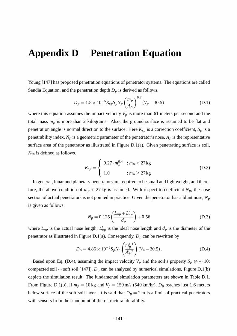
Appendix D Penetration Equation
Young [147] has proposed penetration equations of penetrator systems. The equations are called
Sandia Equation, and the penetration depthDp is derived as follows.
Dp = 1.8×10⁻⁵KspSpNp
(mp
Ap
)0.7
(Vp−30.5) (D.1)
where this equation assumes the impact velocityVp is more than61 meters per second and the
total massmp is more than2 kilograms. Also, the ground surface is assumed to be flat and
penetration angle is normal direction to the surface. HereKsp is a correction coefficient,Sp is a
penetrability index,Np is a geometric parameter of the penetrator’s nose,Ap is the representative
surface area of the penetrator as illustrated in Figure D.1(a). Given penetrating surface is soil,
Ksp is defined as follows.
Ksp =
0.27·m0.4p : mp < 27kg
1.0 : mp≥ 27kg(D.2)
In general, lunar and planetary penetrators are required to be small and lightweight, and there-
fore, the above condition ofmp < 27kg is assumed. With respect to coefficientNp, the nose
section of actual penetrators is not pointed in practice. Given the penetrator has a blunt nose,Np
is given as follows.
Np = 0.125
(Lnp+L′np
dp
)+0.56 (D.3)
whereLnp is the actual nose length,L′np is the ideal nose length anddp is the diameter of the
penetrator as illustrated in Figure D.1(a). Consequently,Dp can be rewritten by
Dp = 4.86×10⁻⁶SpNp
(m1.1
p
A0.7p
)(Vp−30.5) . (D.4)
Based upon Eq. (D.4), assuming the impact velocityVp and the soil’s propertySp (4∼ 10:
compacted soil∼ soft soil [147]),Dp can be analyzed by numerical simulations. Figure D.1(b)
depicts the simulation result. The fundamental simulation parameters are shown in Table D.1.
From Figure D.1(b), ifmp = 10kg andVp = 150m/s (540km/hr), Dp reaches just1.6 meters
below surface of the soft soil layer. It is said thatDp = 2m is a limit of practical penetrators
with sensors from the standpoint of their structural durability.
- 141 -
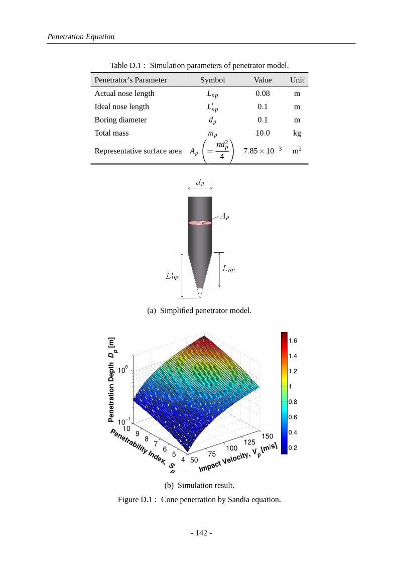
Penetration Equation
Table D.1 : Simulation parameters of penetrator model.
Penetrator’s Parameter Symbol Value Unit
Actual nose length Lnp 0.08 m
Ideal nose length L′np 0.1 m
Boring diameter dp 0.1 m
Total mass mp 10.0 kg
Representative surface areaAp
(=
πd2p
4
)7.85×10⁻³ m2
(a) Simplified penetrator model.
0.2
0.4
0.6
0.8
1
1.2
1.4
1.6
5075
100125
150
45
67
89
1010
−1
100
Penetrability Index, Sp
Pe
ne
tra
tio
n D
ep
th D
p [
m]
Impact Velocity, Vp
[m/s]
(b) Simulation result.
Figure D.1 : Cone penetration by Sandia equation.
- 142 -
Bibliography
Literature related to “Space Science and Space Missions”
[1] S. Fields, A Study of Friction and Adhesion in Simulated Lunar Vacuum,Proceedings of
the 7th Annual Working Group on Extraterrestrial Resources, NASA SP 229, pp. 101-105,
1970.
[2] W. Roepke, Friction Test in Simulated Lunar Vacuum,Proceedings of the 7th Annual Work-
ing Group on Extraterrestrial Resources, NASA SP 229, pp. 107-111, 1970.
[3] G.H. Heiken, D.T. Vaniman and B.M. French,Lunar Sourcebook: A User’s Guide to the
Moon, Cambridge University Press, NY, 1991.
[4] T. Sugano and K. Heki, High Resolution Lunar Gravity Anomaly Map from the Lunar
Prospector Line-of-Sight Acceleration Data,Earth Planets Space, vol. 56, no. 1, pp. 81-
86, 2004.
[5] P. Ulivi and D.M. Harland,Lunar Exploration: Human Pioneers and Robotic Surveyors,
Springer, Paxis Publishing, UK, 2004.
[6] J. Watanabe,Latest Science of the Moon(in Japanese), NHK Books, Japan, 2008.
[7] S. Tanaka, H. Shiraishi, M. Kato and T. Okada, The Science Objectives of the SELENE-II
Mission as the post SELENE Mission,Advances in Space Research, vol. 42, no. 2, pp. 394-
401, 2008.
[8] C.R. Neal, The Moon 35 Years after Apollo: What’s Left to Learn?,Chemie der Erde -
Geochemistry, vol. 69, no. 1, pp. 3-43, 2009.
[9] S. Ulamec, J. Biele and E. Trollope, How to Survive a Lunar Night,Planetary and Space
Science, vol. 58, no. 14-15, pp. 1985-1995, 2010.
[10] http://catless.ncl.ac.uk/Risks/9.24.html#subj3 (accessed on January 5, 2011)
[11] http://www.planetary.org/blog/article/00000987/ (accessed on January 5, 2011)
[12] http://www.jaxa.jp/press/2005/11/20051112hayabusaj.html (in Japanese, accessed on
January 5, 2011)
- 143 -
Bibliography
[13] http://marsrovers.jpl.nasa.gov/mission/statusspiritAll 2009.html#sol1900 (accessed on
January 5, 2011)
[14] http://www.nasa.gov/missionpages/mer/news/mer20100126.html (accessed on January 5,
2011)
Literature related to “Screwed Pile, Auger and Drilling Technique”
[15] O. Schweisgut,Earth Auger, U.S. Patent 1523143, January 13th, 1950.
[16] L.J. Applegate,Earth Boring Machine, U.S. Patent 2509410, May 30th, 1925.
[17] R. Teale, The Concept of Specific Energy of Rock Drilling,International Journal of Rock
Mechanics and Mining Sciences, vol. 2, pp. 57-73, 1965.
[18] S. Hata and N. Ito, Study on Rotary Drilling Mechanism: 2nd Report (in Japanese),Pro-
ceedings of the 9th Annual Meeting, Kansai Chapter of the Japan Society of Civil Engi-
neers, Kyoto, Japan, pp. 223-224, 1967.
[19] The Society of Geotechnical Engineering ed., Soil Mechanics and Foundation Engineering:
Recent Construction Techniques (in Japanese),The Society of Geotechnical Engineering,
Japan, 1967.
[20] H. Raiba, Specific Energy as a Criterion for Drill Performance Prediction,International
Journal of Rock Mechanics and Mining Science & Geomechanics Abstracts, vol. 19,
pp. 39-42, 1982.
[21] A. Ghaly, A. Hanna and M. Hanna, Installation Torque of Screw Anchors in Dry Sand,
Journal of the Japanese Geotechnical Society: Soils and Foundations, vol. 31, no. 2,
pp. 77-92, 1991.
[22] E. Saeki and H. Ohki, A Study of the Screwed Pile -The Results of Installation and Loading
Tests and Analysis of Penetration Mechanism-,Nippon Steel Technical Report, no. 82(7),
pp. 42-50, 2000.
[23] J.W. Slatter, J.P. Seidel and W. Kingwell, A Proposed Model for Soil/Auger Interaction
during Installation of Screw Piling Augers,Proceedings of the 25th Annual Meeting and
Eighth International Conference and Exposition , Deep Foundations Institute, New York,
NY, #897, 2000.
[24] H. Isohata, Historical Study on Iron Pile Foundations and Screw Piles (in Japanese),Pro-
ceedings of the Japan Society of Civil Engineers, vol. 744, no. 4, pp. 139-150, 2003.
- 144 -
Bibliography
[25] W.P. Hong and S.G. Chai, The Skin Friction Capacity of SDA (Separated Doughnut Auger)
Pile, Proceedings of the 13th International Offshore and Polar Engineering Conference,
Honolulu, HI, pp. 740-745, 2003.
[26] F.E. Dupriest and W. L. Koederitz, Maximizing Drill Rates with Real-Time Surveillance
of Mechanical Specific Energy,Proceedings of the 2005 SPE/IADC Drilling Conference,
Amsterdam, The Netherlands, #92194, 2005.
[27] W.L. Koederitz and J. Weis, A Real-Time Implementation of MSE,Proceedings of the
AADE 2005 National Technical Conference and Exhibition, Houston, TX, #AADE-05-
NTCE-66, 2005.
[28] F. Ohsugi, T. Tsuchiya, M. Shimada and K. Yoshida, Pile Installation Tests of Screwed
Piles in A Callibration Chamber (in Japanese),Journal of Structural and Construction
Engineering, Transaction on AIJ, no. 591(5), pp. 69-75, 2005.
[29] M. Koudaet al., Fundamental Study on Penetration and Bearing Capacity of Screw Pile
with Helical Wing (in Japanese),Journal of Structural and Construction Engineering,
Transaction on AIJ, no. 601(3), pp. 91-98, 2006.
[30] H. Fukada, M. Ootsuka, Y. Tanaka and Y. Shioi, Discharging Characteristics by Screw
Auger of Gravel Drain Pile (in Japanese),JSCE Journal of Construction Engineering and
Management, vol. 62, no. 2, pp. 203-212, 2006.
[31] T. Tsuchiya, F. Nakazawa and M. Shimada, Study on Penetration Mechanism of Screw Pile
Based on Soil Movement Around Helical Wing (in Japanese),AIJ Journal of Technology
Design, vol. 13, no. 25(6), pp. 73-76, 2007.
[32] T. Tsuchiya, F. Nakazawa, F. Ohsugi, M. Shimada, Model Tests of Installation and Bearing
Capacity of Screwed Piles (in Japanese),Journal of Structural and Construction Engineer-
ing, Transaction on AIJ, no. 620(10), pp. 75-80, 2007.
[33] M.J. Kaiser, A Survey of Drilling Cost and Complexity Estimation Models,International
Journal of Petroleum Science and Technology, vol. 1, no. 1, pp. 1-22, 2007.
Literature related to “Screw Drive Locomotion/Screw Mechanism”
[34] T.J. Wells, Improvement in the Manner of Constructing and of Propelling Steamboats,
Denominated the “Buoyant Spiral Propeller”, U.S. Patent 2400, December 23rd, 1841.
[35] J.A. Morath,Agricultural Machine, U.S. Patent 635501, October 24th, 1899.
[36] O.A. Hollis, Tractor, U.S. Patent 1069875, August 12th, 1913.
- 145 -
Bibliography
[37] S.M. Code,Amphibious Vehicle, U.S. Patent 1646611, October 25th, 1927.
[38] B.N. Cole, Inquiry into Amphibious Screw Traction,Proceedings of the Institution of Me-
chanical Engineers 1847-1982, vol. 175, no. 19, pp. 919-940, 1961.
[39] U.S. Army,Final Report of Military Potential Test of Marsh Screw Amphibian, USATE-
COM Project, no. 7-5-0524-01-9, Fort Lee, VA, 1964.
[40] M. Neumeyer and B. Jones, The Marsh Screw Amphibian,Journal of Terramechanics,
vol. 2, no. 4, pp. 83-88, 1965.
[41] S.J. Knight, E.S. Rush and B.G. Stinson, Trafficability Tests with the Marsh Screw Am-
phibian,Journal of Terramechanics, vol. 2, no. 4, pp. 31-50, 1965.
[42] J.J. De Bakker,De Bakker Amphibian Vehicle, U.S. Patent 3333563, August 1st, 1967.
[43] H. Dugoff and I. Ehrlich, Model Tests of Buoyant Screw Rotor Configurations,Journal of
Terramechanics, vol. 4, no. 3, pp. 9-22, 1967.
[44] W.K. Fales, D.W. Amick and B.G. Schreiner, The Riverine Utility Craft (RUC),Journal of
Terramechanics, vol. 8, no. 3, pp. 23-38, 1972.
[45] E.S. Rush and W.E. William,Evaluation of the Marsh Screw Amphibian (MSA), Technical
Report: Evaluation of Herbicide Application Platforms for Use in Aquatic Plant Control,
no. A-77-1, Washington, DC, 1977.
[46] C.A. Pickover, Mathematics and Beauty: A Sampling of Spirals and ‘Strange’ Spirals in
Science, Nature and Art,Leonardo, vol. 21, no. 2, pp. 173-181, 1988.
[47] Z. Kembłowski, J. Sek and P. Budzynski The Concept of a Rotational Rheometer with
Helical Screw Impeller,Rheologica Acta, vol. 27, no. 1, pp. 82-91, 1988.
[48] M. Sendoh, N. Ajiro, K. Ishiyama, M. Inoue and K. I. Arai, Effect of Machine Shape on
Swimming Properties of the Spiral-Type Magnetic Micro-Machine,IEEE Transactions on
Magnetics, vol. 35, no. 5, pp. 3688-3690, 1999.
[49] A.W. Roberts, The Influence of Granular Vortex Motion on the Volumetric Performance of
Enclosed Screw Conveyors,Powder Technology, vol. 104, no. 1, pp. 56-67, 1999.
[50] C. Rorres, The Turn of the Screw: Optimal Design of an Archimedes Screw,ASCE Journal
of Hydraulic Engineering, vol. 126, no. 1, pp. 72-80, 2000.
[51] K. Ishiyama, M. Sendoh, A. Yamazaki and K. Arai, Swimming Micro-machine Driven by
Magnetic Torque,Sensors and Actuators A: Physical, vol. 91, no. 1-2, pp. 141-144, 2001.
- 146 -
Bibliography
[52] A. Yamazaki, M. Sendoh, K. Ishiyama, T. Hayase and K. Arai, Three-dimensional Analysis
of Swimming Properties of a Spiral-type Magnetic Micro-machine,Sensors and Actuators
A: Physical, vol. 105, no. 1, pp. 103-108, 2003.
[53] T. Koetsier and H. Blauwendraat, The Archimedean Screw-Pump: A Note on Its Invention
and the Development of the Theory,Proceedings of the 2004 International Symposium on
History of Machines and Mechanisms, Cassino, Italy, pp. 181-194, 2004.
[54] M.E. Rentschleret al., Modeling, Analysis, and Experimental Study of In Vivo Wheeled
Robotic Mobility, IEEE Transactions on Robotics, vol. 22, no. 2, pp. 308-321, 2006
[55] M.E. Rentschler, S.M. Farritor and K.D. Iagnemma, Mechanical Design of Robotic In Vivo
Wheeled Mobility,ASME Journal of Mechanical Design, vol. 129, pp. 1037-1045, 2007.
[56] A. Fuchs and H. Zangl, Measuring Flow Parameters of Particulate and Powdery Solids in
Industrial Transportation Processes,International Journal on Smart Sensing and Intelligent
Systems, vol. 1, no. 2, pp. 388-402, 2008.
[57] M. Ogata, Y. Shimotsuma and N. Shiotsu, Origin of the Concept of Screws (in Japanese),
Transactions of the Japan Society of Mechanical Engineers, Series C, vol. 74, no. 746,
pp. 2356-2362, 2008.
[58] P.J. Owen and P.W. Cleary, Prediction of Screw Conveyor Performance Using the Discrete
Element Method (DEM),Powder Technology, vol. 193, no. 3, pp. 274-288, 2009.
[59] S. Yim and D. Jeon, Capsular Microrobot Using Directional Friction Spiral,Proceedings
of the 2009 IEEE International Conference on Robotics and Automation, Kobe, Japan,
pp. 4444-4449, 2009.
[60] M. Shikanaiet al., Development of a Robotic Endoscope that Locomotes in the Colon
with Flexible Helical Fins,Proceedings of the 31st Annual International Conference of the
IEEE/EMBS, Minneapolis, MN, pp. 5126-5129, 2009.
[61] T.C. Lexen,Screw Driven Mobile Base, U.S. Patent 20090044990, February 19th, 2009.
[62] J. Lee, B. Kim and Y. Hong, A Flexible Chain-based Screw Propeller for Capsule Endo-
scopes,International Journal of Precision Engineering and Manufacturing, vol. 10, no. 4,
pp. 27-34, 2009.
[63] Q. Liu et al., Development of a Spiral Propulsion Mechanism in Wetlands-Relation be-
tween Torque and Load,Memoirs of the Muroran Institute of Technology, vol. 59, pp. 133-
135, 2010.
- 147 -
Bibliography
[64] L. Juet al., Experimental Results of a Novel Amphibian Solution for Aquatic Robot,Pro-
ceedings of the 2010 IEEE International Conference on Robotics and Automation, Anchor-
age, AK, pp. 2261-2266, 2010.
[65] M. Ceccarelli,The Mechanics of Archimedes Towards Modern Mechanism Design, in “The
Genius of Archimedes -- 23 Centuries of Influence on Mathematics, Science and Engineer-
ing” , Springer, The Netherlands, pp. 177-187, 2010.
Literature related to “Locomotion Mechanics on Soil (Terramechanics)”
[66] M.G. Bekker,Theory of Land Locomotion, University of Michigan Press, MI, 1956.
[67] Z.J. Janosi and B. Hanamoto, The Analytical Determination of Drawbar Pull as A Function
of Slip for Tracked Vehicle,Proceedings of the 1st International Conference on Terrain-
Vehicle Systems, Turin, Italy, pp. 707-736, 1961.
[68] Z.J. Janosi,Performance Analysis of a Driven Non-Deflecting Tire in Soil, U.S. Army
Tank-Automotive Center, Land Locomotion Laboratory, Warren, MI, 1963.
[69] E. Hegedus, Pressure Distribution and Slip-Sinkage Relationship Under Driven Rigid
Wheels,U.S. Army Tank-Automotive Center, Land Locomotion Laboratory, no. 88, War-
ren, MI, 1963.
[70] J.Y. Wong and A.R. Reece, Prediction of Rigid Wheel Performance based on the Analysis
of Soils - Wheel Stresses Part I. Performance of Driven Rigid Wheels,Journal of Terrame-
chanics, vol. 4, no. 1, pp. 81-98, 1967.
[71] O. Onafeko and A.R. Reece, Soil Stresses and Deformations beneath Rigid Wheels,Jour-
nal of Terramechanics, vol. 4, no. 1, pp. 59-80, 1967.
[72] H. Schwanghart, Lateral Forces on Steered Tyres in Loose Soil,Journal of Terramechanics,
vol. 5, no. 1, pp. 9-29, 1968.
[73] M.G. Bekker,Introduction of Terrain-Vehicle Systems, University of Michigan Press, MI,
1969.
[74] N. Costes and W. Trautwein, Elastic Loop Mobility System: A New Concept for Planetary
Exploration,Journal of Terramechanics, vol. 10, no. 1, pp. 89-104, 1973.
[75] S. Hata,Construction Machinery(in Japanese), Kashima Publishing, Japan, 1987.
[76] D.A. Crolla and A.S.A. El-Razaz, A Review of the Combined Lateral and Longitudinal
Force Generation of Tyres on Deformable Surfaces,Journal of Terramechanics, vol. 24,
no. 3, pp. 199-225, 1987.
- 148 -
Bibliography
[77] X.L. Wang, T. Tanaka and M. Yamazaki, Study on Soil-Lugged Wheel Interaction: Part 1
-Dynamic Behaviour of a Lugged Wheel- (in Japanese),Journal of the Japanese Society
of Agriculture Machinery, vol. 51, no. 3, pp. 33-40, 1989.
[78] A. Oida, A. Satoh, H. Itoh and K. Triratanasirichai, Three-dimensional Stress Distributions
on a Tire-Sand Contact Surface,Journal of Terramechanics, vol. 28, no. 4, pp. 319-330,
1991.
[79] Z. Jide, W. Zhixin and L. Jude , The Way to Improve the Trafficability of Vehicles on
Sand,Proceedungs of the 5th European Conference on Terrain-Vehicle Systems, Budapest,
Hungary, pp. 121-126, 1991.
[80] J.A. Okello, Prediction of the Force Distribution between the Soil and a Pneumatic Wheel,
Journal of Agricultural Engineering Research, vol. 51, pp. 249-262, 1992.
[81] B.E. Wallace and N.S. Rao, Engineering Elements for Transportation on the Lunar Surface,
Applied Mechanics Review, vol. 46, no. 6, pp. 301-312, 1993.
[82] J.Y. Wong,Theory of Ground Vehicles (3rd ed.), John Wiley & Sons, Inc., NY, 2001.
[83] T. Muro and J. O’Brien,Terramechanics, A.A. Balkema Publishers, The Netherlands,
2004.
[84] K. Iagnemma and S. Dubowsky,Mobile Robots in Rough Terrain, Springer, NY, 2005.
[85] J.Y. Wong and W. Huang, Wheels vs. Tracks -A Fundamental Evaluation from the Traction
Perspective,Journal of Terramechanics, vol. 43, no. 1, pp. 27-42, 2006.
[86] A. Miwa, G. Ishigami, K. Nagatani and K. Yoshida, Terramechanics-Based Analysis on
Climbing Ability of a Lunar/Planetary Exploration Rover (in Japanese),Proceedings of
the 11th Robotics Symposia, Saga, Japan, pp. 514-519, 2006.
[87] L. Ojeda, D. Cruz, G. Reina and J. Borenstein, Current-Based Slippage Detection and
Odometry Correction for Mobile Robots and Planetary Rovers,IEEE Transactions on
Robotics, vol. 22, no. 2, pp. 366-378, 2006.
[88] C.A. Brooks, K.D. Iagnemma and S. Dubowsky, Visual Wheel Sinkage Measurement for
Planetary Rover Mobility Characterization,Autonomous Robots, vol. 21, no. 1, pp. 55-64,
2006.
[89] S. Hutangkabodee, Y.H. Zweiri, L.D. Seneviratne and K. Althoefer, Soil Parameter Iden-
tification for Wheel-terrain Interaction Dynamics and Traversability Prediction,Interna-
tional Journal of Automation and Computing, vol. 3, no. 3, pp. 244-251, 2006.
- 149 -
Bibliography
[90] G. Ishigami, A. Miwa, K. Nagatani and K. Yoshida, Terramechanics-based Model for
Steering Maneuver of Planetary Exploration Rovers on Loose Soils,Journal of Field
Robotics, vol. 24, no. 3, pp. 233-250, 2007.
[91] H. Nakashima and Y. Takatsu, Analysis of Tire Tractive Performance on Deformable Ter-
rain by Finite Element-Discrete Element Method,Journal of Computational Science and
Technology, vol. 2, no. 4 pp. 423-434, 2008.
[92] J. Yamakawa, O. Yoshimura and K. Watanabe, Development of Tire Model on Dry Sand
by Model Size Experiment: First Report (in Japanese),Transactions of the Society of Au-
tomotive Engineers of Japan, vol. 39, no. 6, pp. 41-46, 2008.
[93] K. Iizuka, Y. Kunii and T. Kubota, Study on Wheeled Forms of Lunar Robots Considering
Elactic Characteristic for Traversing Soft Terrain: Effect of Elastic Wheel Considering in
Interaction Between Wheel and Soft Soil (in Japanese),Transactions of the Japan Society
of Mechanical Engineers, Series C, vol. 74, no. 748, pp. 2962-2967, 2008.
[94] G. Ishigami, K. Nagatani and K. Yoshida, Slope Traversal Controls for Planetary Explo-
ration Rover on Sandy Terrain,Journal of Field Robotics, vol. 26, no. 3, pp. 264-286,
2009.
[95] L.E. Ray, Estimation of Terrain Forces and Parameters for Rigid-Wheeled Vehicles,IEEE
Transactions on Robotics, vol. 25, no. 3, pp. 717-726, 2009.
[96] M. Scharringhausen, D. Beermann, O. Kromer and L. Richter, Wheel-Soil Interaction
Model for Planetary Rover Vehicles,Proceedings of the 11th European Conference of the
International Society for Terrain-Vehicle Systems, Bremen, Germany, #P75, 2009.
[97] M. Lyasko, Slip Sinkage Effect in Soil-Vehicle Mechanics,Journal of Terramechanics,
vol. 47, no. 1, pp. 21-31, 2010.
[98] V.K. Tiwari, K.P. Pandey and P.K. Pranav, A Review on Traction Prediction Equations,
Journal of Terramechanics, vol. 47, no. 3, pp. 191-199, 2010.
[99] L. Ding, H. Gao, Z. Deng and J. Tao, Wheel Slip-Sinkage and its Prediction Model of
Lunar Rover,Journal of Central South University of Technology, vol. 17, no. 1, pp. 129-
135, 2010.
Literature related to “Soil Mechanics”
[100] E. Hegedus, A Simplified Method for the Determination of Bulldozing Resistance,Land
Locomotion Research Laboratory, U.S. Army Tank Automotive Command Report, vol. 61,
Warren, MI, 1960.
- 150 -
Bibliography
[101] R.W. Clough, The Finite Element Method in Plane Stress Analysis,Proceedings of the
2nd ASCE Conference on Electronic Computation, Pittsburg, PA, USA, pp. 345-378, 1960.
[102] A. Schofield and P. Wroth,Critical State Soil Mechanics, McGraw-Hill Education, UK,
1968.
[103] P.A. Cundall and O.D.L. Strack, A Discrete Numerical Model for Granular Assemblies,
Geotechnique, vol. 29, no. 1, pp. 47-65, 1979.
[104] M. Hirota, T. Oshima and Y. Sugihara, Shear Test of Powder Bed in the Tensile Stress
Regions (in Japanese),Journal of the Society of Powder Technology, vol. 18, no. 9, pp. 678-
680, 1981.
[105] J. Carter, J. Booker and S. Yeung, Cavity Expansion in Cohesive Frictional Soils,
Geotechnique, vol. 36, no. 3, pp. 349-358, 1986.
[106] K. Ito, S. Katsuki, N. Ishikawa, S. Abe and T. Nakamura, Shear Resistance of Filled
Material in Check Dam (in Japanese),Journal of the Japan Society of Erosion Control
Engineering, vol. 50, no. 1, pp. 3-14, 1997.
[107] H. Kanamori, S. Udagawa, T. Yoshida, S. Matsumoto and K. Takagi, Properties of Lunar
Soil Simulant Manufactured in Japan,Proceedings of the 6th International Conference
and Exposition on Engineering Construction, and Operations in Space, Albuquerque, NM,
USA, pp. 462-468, 1998.
[108] S.H. Yu,Cavity Expansion Methods in Geomechanics, Kluwer Academic Publishers, UK,
2000.
[109] O. Kusakabe,Soil Mechanics(in Japanese), Korona Publishing, Japan, 2004.
[110] Lunarant producted by WEL RESEARCH Co., Ltd. (http://www.wel.co.jp/product.html,
accessed on January 5, 2011)
[111] Report on Inorganic Recyclable Resource (Coal Ash & Iron and Steel Slag), Chapter 2,
Hokkaido, Japan, 2004. (in Japanese, http://edb.hokkaido-ies.go.jp/edb/junkan/junkankyo
manual/kensetsu-manual15/kensetsu-manual15-2-1.pdf, accessed on January 5, 2011)
Literature related to “Field Robotics and Space Exploration Rover”
[112] http://www.britishmuseum.org/explore/highlights/highlightobjects/me/t/thestandard
of ur.aspx (accessed on January 5, 2011)
[113] S. Kassel,Lunokhod-1 Soviet Lunar Surface Vehicle, LAND Report, no. R-802-ARPA,
The Land Corporation, Santa Monica, CA, 1971.
- 151 -
Bibliography
[114] B. Ilon, Directionally Stable Self-propelled Vehicle, U.S. Patent 3746112, July 17th, 1971.
[115] A Roving Lunokhod Explores the Moon, 53: Society for Science & the Public,Science
News, vol. 103, no. 4, 1973. (http://www.jstor.org/stable/pdfplus/3957956, accessed on
January 5, 2011)
[116] A. Kemurdjianet al., Soviet Developments of Planet Rovers in Period of 1964∼1990,
Journal of the Robotics Society of Japan, vol. 12, no. 7, pp. 75-83, 1994. (translated into
Japanese)
[117] L. Matthieset al., Mars Microrover Navigation: Performance Evaluation and Enhance-
ment,Autonomous Robotics, vol. 2, no. 4, 1995.
[118] A.L. Kemurdjian, Planet Rover as an Object of the Engineering Design Work,Proceed-
ings of the 1998 IEEE International Conference on Robotics and Automation, Leuven,
Belgium, pp. 140-145, 1998.
[119] K. Yoshida, Robotics for Space Exploration (in Japanese),Journal of the Society of In-
strument and Control Engineers, vol. 39, no. 9, pp. 576-580, 2000.
[120] K. Kotay and D. Rus, The Inchworm Robot: A Multi-Functional System,Autonomous
Robots, vol. 8, no. 1, pp. 53-69, 2000.
[121] T. Yoshimitsu, T. Kubota and I. Nakatani, New Mobility System of Exploration Rover for
Small Planetary Bodies (in Japanese),Journal of the Robotics Society of Japan, vol. 18,
no. 2, pp. 292-299, 2000.
[122] B. Kennedyet al., LEMUR: Legged Excursion Mechanical Utility Rover,Autonomous
Robots, vol. 11, pp. 201-205, 2001.
[123] R. Roncoli and J. Ludwinski, Mission Design Overview for the Mars Exploration Rover
Mission, Proceedings of the 2002 AIAA/AAS Astrodynamics Specialist Conference and
Exhibit, Monterey, CA, USA, #AIAA 2002-4823, 2002.
[124] S.W. Squyreset al., Athena Mars Rover Science Investigation,Journal of Geophysical
Research, vol. 108, no. E12, p.8062, 2003.
[125] B. Harrington and C. Voorhees, The Challenges of Designing the Rocker-Bogie Sus-
pension for the Mars Exploration Rover,Proceedings of the 37th Aerospace Mechanisms
Symposium, Houston, TX, pp. 185-196, 2004.
[126] S.W. Squyreset al., Two Years at Meridiani Planum: Results from the Opportunity Rover,
Science, vol. 313, no. 5792, pp. 1403-1407, 2006. (http://www.sciencemag.org/cgi/content/
full/313/5792/1403, accessed on January 5, 2011)
- 152 -
Bibliography
[127] T. Nakamura, T. Kato, T. Iwanaga and Y. Muranaka, Development of a Peristaltic Crawl-
ing Robot Based on Earthworm Locomotion,Journal of Robotics and Mechatronics,
vol. 18, no. 3, pp. 229-304, 2006.
[128] P. Ulivi and D.M. Harland,Robotic Exploration of the Solar System: Part 1 The Golden
Age 1957-1982, Springer, Paxis Publishing, UK, 2007.
[129] B. Wilcox et al., ATHLETE: A Cargo Handling and Manipulation Robot for the Moon,
Journal of Field Robotics, vol. 24, no. 5, pp. 421-434, 2007.
[130] A. Gfrerrer, Geometry and Kinematics of the Mecanum Wheel,Computer Aided Geomet-
ric Design, vol. 25, no. 9, pp. 784-791, 2008.
[131] E. Rohmer, G. Reina, G. Ishigami, K. Nagatani and K. Yoshida, Action Planner of Hy-
brid Leg-Wheel Robots for Lunar and Planetary Exploration,Proceedings of the 2008
IEEE/RSJ International Conference on Intelligent Robots and Systems, Nice, France,
pp. 3902-3907, 2008.
[132] K. Tadakumaet al., Crawler Vehicle with Circular Cross-Section Unit to Realize Side-
ways Motion,Proceedings of the 2008 IEEE/RSJ International Conference on Intelligent
Robots and Systems, Nice, France, pp. 2422-2428, 2008.
[133] C.M. Gifford, A. Agah, B.L. Carmichael, U.B. Wade and I. Ruiz, Seismic TETwalker
Mobile Robot Design and Modeling,Proceedings of the IEEE International Conference
on Technologies for Practical Robot Applications 2008, Woburn, MA, pp. 7-12, 2008.
[134] S. Ransom, O. Kromer and M. Luckemeier, Planetary Rovers with Mecanum Wheels,
Proceedings of the 10th ESA Workshop on Advanced Space Technologies for Robotics and
Automation, Noordwijk, The Netherlands, #14-04, 2008.
[135] A. Schieleet al., Nanokhod Exploration Rover: A Rugged Rover Suited for Small, Low-
Cost, Planetary Lander Mission,IEEE Robotics & Automation Magazine, vol. 15, no. 2,
pp. 96-107, 2008.
[136] S. Wakabayashi, H. Sato and S. Nishida, Design and Mobility Evaluation of Tracked
Lunar Vehicle,Journal of Terramechanics, vol. 46, no. 3, pp. 105-114, 2009.
[137] R.A. Kerr, Mars Rover Trapped in Sand, But What Can End a Mission?,Science, vol. 324,
no. 5930, p.998, 2009. (http://www.sciencemag.org/cgi/content/full/324/5930/998, ac-
cessed on January 5, 2011)
[138] S.W. Squyreset al., Exploration of Victoria Crater by the Mars Rover Opportunity,Sci-
ence, vol. 324, no. 5930, pp. 1058-1061, 2009. (http://www.sciencemag.org/cgi/content/
full/324/5930/1058, accessed on January 5, 2011)
- 153 -
Bibliography
[139] H. Kinoshita, K. Nagatani and K. Yoshida, Development of a Small-sized Leg-Track
Robot to Traverse on Loose Slopes and Irregular Terrains (in Japanese),Proceedings of the
2010 JSME Annual Conference on Robotics and Mechatronics, Asahikawa, Japan, #2A1-
E25, 2010.
Literature related to “Lunar and Planetary Sampling Technique”
[140] M.V. Winnendael and G. Visentin, Nanokhod Microrover Heading Towards Mars,Pro-
ceedings of the 5th International Symposium on Artificial Intelligence, Robotics and Au-
tomation in Space, Noordwijk, The Netherlands, pp. 69-76, 1999.
[141] T. Muff, L. Johnson, R. King and B. M. Duke, A Prototype Bucket Wheel Excavator
for the Moon, Mars and Phobos,Space Technology and Applications International Forum
2004, AIP Proceedings, Albuquerque, NM, vol. 699, pp. 967-974, 2004.
[142] S. Mukherjee, P. Brian, B. Glass, J. Guerrero and S. Stanley, Technologies for Exploring
the Martian Subsurface,Proceedings of the 2006 IEEE Aerospace Conference, Big Sky,
MT, #1349, 2006.
[143] E. Reet al., EXOMARS: Two Meters Depth Drilling,Proceedings of the 59th Interna-
tional Astronautical Congress, Glasgow, Scotland, #A3.3-B7, 2008.
[144] J. Crabtree, J.L. Klosky, R. Gash and D. Miller, Helical Ancors: Lateral Resistance For
Shaping The Lunar Surface,Proceedings of the Earth & Space 2008, Long Beach, CA,
#7458, 2008.
[145] P.W. Bartlett, D. Wettergreen, W.L. Whittaker, Design of the Scarab Rover for Mobility
& Drilling in the Lunar Cold Traps,Proceedings of the 9th International Symposium on
Artificial Intelligence, Robotics and Automation in Space, Los Angeles, CA, #m145, 2008.
[146] R. Bonitzet al., The Phoenix Mars Lander Robotic Arm,Proceedings of the 2009 IEEE
Aerospace Conference, Big Sky, MT, #1695, 2009.
Literature related to “Penetration Technology”
[147] C.W. Young, Penetration Equations,SANDIA Laboratories Report, #SAND97-2426,
1997.
[148] T. Nakajimaet al., Lunar Penetrator Program: LUNAR-A,Acta Astronautica, vol. 39,
no. 1-4, pp. 111-119, 1996.
[149] Y.A. Surkov and R.S. Kremnev, Mars-96 Mission: Mars Exploration with the Use of
Penetrators,Planetary Space Science, vol. 46, no. 11, pp. 1689-1696, 1998.
- 154 -
Bibliography
[150] H. Mizutani, A. Fujimura, M. Hayakawa, S. Tanaka and H. Shiraishi, Understanding of
Lunar Interior by Penetrators (in Japanese),Journal of the Japan Society fot Precision
Engineering, vol. 63, no. 10, pp. 1346-1350, 1997.
[151] R.D. Lorenza, J.E. Moersch, J.A. Stone, A.R. MorganJr and S.E. Smrekar, Penetration
Tests on the DS-2 Mars Microprobes: Penetration Depth and Impact Accelerometry,Plan-
etary and Space Science, vol. 48, pp. 419-436, 2000.
[152] Y. Gao, A. Ellery, M. Jaddou, J. Vincent and S. Eckersley, Planetary Micro-Penetrator
Concept Study with Biomimetric Drill and Sampler Design,IEEE Transactions on
Aerospace and Electronics Systems, vol. 43, no. 3, pp. 875-885, 2007.
Literature related to “Subsurface Drilling Robot”
[153] K. Tomio, H. Igarashi and A. Harada, A Proposal of the Earthworm Rover for Exploring
the Moon (in Japanese),Proceedings of the Annual Conference of the Japanese Society for
the Science of Design, vol. 46, pp. 316-317, 1999.
[154] T. Kudo, K. Yoshida, Basic Examen by Mole-Type Moon Excavation Robot (in Japanese),
Proceedings of the 183th Symposium, Tohoku Chapter of the Society of Instrument and
Control Engineers, Tokyo, Japan, #183-6, 1999.
[155] L. Richter, H. Kochan, V. Gromov and P. Coste, The Development of the “Mole with
Sampling Mechanism” Subsurface Sampler,Proceedings of the 6th ESA Workshop on Ad-
vanced Space Technologies for Robotics and Automation, Noordwijk, The Netherlands,
#3.5a-3, 2000.
[156] K. Tateyama, An Idea for a Tunnel Boring Machine without Thrust Force (in Japanese),
Terramechanics, vol. 20, pp. 29-32, 2000.
[157] K. Yoshida, T. Kudo, Y. Kawakatsu, T. Yokoyama and M. Sonoyama, Development of a
Mole-like Robot for Lunar Subserface Exploration (in Japanese),Proceedings of the 2000
JSME Annual Conference on Robotics and Mechatronics, Kumamoto, Japan, #1P1-07-
019, 2000.
[158] K. Tomio, H. Igarashi and A. Harada, The Robot Using Movement Mechanism of Earth-
worm (in Japanese),Proceedings of the Annual Conference of the Japanese Society for the
Science of Design, vol. 47, pp. 198-199, 2000.
[159] W. Zimmerman, R. Bonitz and J. Feldman, Cryobot: An Ice Penetrating Robotic Vehicle
for Mars and Europa,Proceedings of the 2001 IEEE Aerospace Conference, Big Sky, MT,
vol. 1, pp. 311-323, 2001.
- 155 -
Bibliography
[160] N. Mizuno and K. Yoshida, Development of a Robot Prototype for Excavation and Explo-
ration of the Moon and Planet (in Japanese),Proceedings of the 199th Symposium, Tohoku
Chapter of the Society of Instrument and Control Engineers, Miyagi, Japan, #199-3, 2001.
[161] L. Richteret al., Development and Testing of Subsurface Sampling Devices for the Beagle
2 Lander,Planetary and Space Science, vol. 50, no. 9, pp. 903-913, 2002.
[162] K. Yoshida et al., Development of Mole-type Robot for Lunar/Planetary Sub-Surface
Exploration, and its Performance Evaluation (in Japanese),Proceedings of the 20th Annual
Conference of Robotics Society of Japan, Osaka, Japan, #1J35, 2002.
[163] K. Watanabe, S. Shimoda, T. Kubota and I. Nakatani, A Mole-Type Drilling Robot for
Lunar Subsurface Exploration,Proceedings of the 7th International Symposium on Artifi-
cial Intelligence, Robotics and Automation in Space, Nara, Japan, #AS-7, 2003.
[164] S.P. Gorevanet al., Strategies for Future Mars Exploration: An Infrastructure for the
Near and Longer Term Future Exploration of the Subsurface of Mars,Proceedings of the
6th International Conference on Mars, Pasadena, CA, #3196, 2003.
[165] L. Richter, P. Coste, V. Gromov and A. Grzesik, The Mole with Sampling Mechanism
(MSM)- Technology Development and Payload of Beagle 2 Mars Lander,Proceedings
of the 8th ESA Workshop on Advanced Space Technologies for Robotics and Automation,
Noordwijk, The Netherlands, #I-11, 2004.
[166] R. Campaciet al., Design and Optimization of A Terrestrial Guided Mole for Deep Sub-
soil Exploration-Boring Performance Experimental Analysis,Proceedings of the 8th In-
ternational Symposium on Artificial Intelligence, Robotics and Automation in Space, (ESA
SP-603), Munich, Germany, #4a-1, 2005.
[167] Y. Liu, B. Weinberg and C. Mavroidis, Design and Modeling of the NU Smart Space
Drilling System (SSDS),Proceedings of the 10th ASCE Aerospace Division Interna-
tional Conference Engineering, Construction, and Operations in Challenging Environ-
ments (Earth&Space 2006), vol. 188, #96, Houston, TX, 2006.
[168] Y. Liu, B. Weinberg and C. Mavroidis, Mechanical Design and Modeling of A Robotic
Planetary Drilling System,Proceedings of the ASME 2006 International Design Engi-
neering Technical Conference & Computers in Engineering Conference, Philadelphia, PA,
#DETC2006-99699, 2006.
[169] T.M. Myrick and S. Gorevan,Self-Propelled Instrumented Deep Drilling System, U.S.
Patent 7055625, June 6th, 2006.
- 156 -
Bibliography
[170] C.R. Stoker, A. Gonzales, J.R. Zavaleta, Moon/Mars Underground Mole,Proceedings of
the 2007 NASA Science Technology Conference, Adelphi, MD, #C10P1, 2007.
[171] S. Yasuda and K. Komatsu, Regolith Drilling Mechanism using Reaction Torque (in
Japanese),Proceedings of the 2008 JSME Annual Conference on Robotics and Mecha-
tronics, Nagano, Japan, #2P2-A20, 2008.
[172] T. Seidlet al., Bio-inspiration from Plants’ Roots,ARIADNA Study 06/6301, 2008.
[173] S. Yasuda,Autonomous Excavation Apparatus, U.S. Patent 20090188137, July 30th,
2009.
[174] Y. Bar-Cohen and K. Zacny,Drilling in Extreme Environments, Wiley-VCH, Weinheim,
Germany, 2009.
[175] S. Yasuda and K. Komatsu, Research for Regolith Drilling Mechanism Using Reactive
Torque (in Japanese),Proceedings of the 18th Space Engineering Conference, Tokyo,
Japan, #D3, 2010.
[176] B. Mazzolaiet al., A Miniaturized Mechatronic System Inspired by Plant Roots for Soil
Exploration, IEEE/ASME Transactions on Mechatoronics, vol. 16, no. 2, pp. 201-212,
2011.
[177] A. Koller-Hodac et al., Actuated Bivalve Robot Study of the Burrowing Locomotion
in Sediment,Proceedings of the 2010 IEEE International Conference on Robotics and
Automation, Anchorage, Alaska, USA, pp. 1209-1214, 2010.
[178] H. Omori, T. Murakami, H. Nagai, T. Nakamura and T. Kubota, An Earth Auger as Exca-
vator for Planetary Underground Explorer Robot Using Peristaltic Crawling,Proceedings
of the 10th International Symposium on Artificial Intelligence, Robotics and Automation in
Space, Sapporo, Japan, pp. 784-789, 2010.
[179] T. Murakami, H. Omori, H. Nagai and T. Nakamura, Development of Lunar Underground
Explorer Robot using Peristaltic Crawling of Earthworm (in Japanese),Proceedings of the
28th Annual Conference of Robotics Society of Japan, Nagoya, Japan, #RSJ2010AC3G2-6,
2010.
[180] S. Yasuda and K. Komatsu, Research of Sensor Burying Mechanism (in Japanese),Pro-
ceedings of the 54th Symposium on Space Sciences and Technology, Shizuoka, Japan,
#JSASS-2010-4405, 2010.
[181] R.A. Russel, CRABOT: A Biomimetic Burrowing Robot Designed for Underground
Chemical Source Location,Advanced Robotics, vol. 25, no. 1-2, pp. 119-134, 2011.
- 157 -

Bibliography
- 158 -
Publications
Journal Papers
• Kenji Nagaoka, Takashi Kubota, Masatsugu Otsuki and Satoshi Tanaka, “An Exper-
imental Study on Contra-Rotor Screw Drilling Mechanism: Effective Screw Mech-
anism for Lunar Subsurface Exploration Robot” (in Japanese),Transactions of the
Japan Society of Mechanical Engineers, Series C, vol. 75, no. 758, pp. 2295-2300,
2009.
• Kenji Nagaoka, Takashi Kubota, Masatsugu Otsuki and Satoshi Tanaka, “Experi-
mental Analysis of Screw Drilling Mechanism for Lunar Robotic Subsurface Explo-
ration”, Advanced Robotics, vol. 24, no. 8-9, pp. 1127-1147, 2010.
Reviewed International Conference Presentations
• Kenji Nagaoka, Takashi Kubota, Ichiro Nakatani and Satoshi Tanaka, “Drilling Mech-
anism of Autonomous Burrowing Robot for Lunar Subsurface Exploration”,9th In-
ternational Symposium on Artificial Intelligence, Robotics and Automation in Space,
#m063, 2008.
• Kenji Nagaoka, Takashi Kubota and Satoshi Tanaka, “Experimental Study on Au-
tonomous Robotic Screw Burrower for Lunar and Planetary Subsurface Exploration”,
2008 IEEE/RSJ International Conference on Intelligent Robotics and Systems, pp. 4104-
4109, 2008.
• Kenji Nagaoka, Takashi Kubota, Masatsugu Otsuki and Satoshi Tanaka, “Robotic
Screw Explorer for Lunar Subsurface Investigation: Dynamics Modelling and Ex-
perimental Validation”,14th International Conference on Advanced Robotics, #28,
2009.
• Kenji Nagaokaand Takashi Kubota, “Analytic Study on Screw Drilling Mechanism”,
2009 IEEE International Conference on Robotics and Biomimetics, pp. 1579-1584,
2009.
- 159 -
Publications
• Kenji Nagaokaand Takashi Kubota, “Modeling and Analysis on Exploration Rover
with Screw Drive Mechanism over Loose Soil”,10th International Symposium on
Artificial Intelligence, Robotics and Automation in Space, pp. 162-169, 2010.
• Kenji Nagaokaand Takashi Kubota, “Maneuverability of Mobile Robot Driven by
Archimedean Screw Units on Sand”,Joint 9th Asia-Pacific ISTVS Conference and
Annual Meeting of the Japanese Society for Terramechanics, #086-0042, 2010.
• Kenji Nagaoka, Masatsugu Otsuki, Takashi Kubota and Satoshi Tanaka, “Terramechanics-
based Propulsive Characteristics of Mobile Robot Driven by Archimedean Screw
Mechanism on Soft Soil”,2010 IEEE/RSJ International Conference on Intelligent
Robots and Systems, pp. 4946-4951, 2010.
Reviewed National Conference Presentations
• Kenji Nagaoka, Takashi Kubota and Satoshi Tanaka, “Non-Reaction Excavation Mech-
anism for Subsurface Exploration Robot” (in Japanese),13th Robotics Symposia,
pp. 224-229, 2008.
• Kenji Nagaoka, Takashi Kubota, Masatsugu Otsuki and Satoshi Tanaka, “Develop-
ment of Subsurface Burrowing Explorer Using Screw Mechanism: Derivation of
Theoretical Model Based on Soil Mechanics” (in Japanese),14th Robotics Symposia,
pp. 173-178, 2009.
• Kenji Nagaokaand Takashi Kubota, “Mobility of Screw Drive Rover on Soft Ground
Based on Soil Interaction Model” (in Japanese),15th Robotics Symposia, pp. 173-
178, 2010.
• Kenji Nagaoka, Takashi Kubota and Kojiro Iizuka, “Trafficability Characterization
of an Archimedean Screw Unit on Sand” (in Japanese),16th Robotics Symposia,
2011. (to appear)
National Conference Presentations
• Kenji Nagaoka, Keisuke Watanabe, Masatsugu Otsuki, Satoshi Tanaka and Takashi
Kubota, “Primal Study on Burrowing Subsurface Exploration Robot” (in Japanese),
7th Space Science Symposium, #P3-43, 2006.
• Kenji Nagaoka, Edmond So, Takashi Kubota, Masatsugu Otsuki and Satoshi Tanaka,
“Study on Subsurface Exploration Robot” (in Japanese),2007 JSME Annual Con-
ference on Robotics and Mechatronics, #2A2-M06, 2007.
- 160 -
Publications
• Kenji Nagaoka, Satoshi Tanaka and Takashi Kubota, “Study on Excavation Mech-
anism for Lunar Subsurface Exploration by Burrowing Robot”,17th Workshop on
JAXA Astrodynamics and Flight Mechanics, pp. 380-385, 2007.
• Kenji Nagaokaand Takashi Kubota, “N-RDM System of Burrowing Robot for Lu-
nar Subsurface Exploration” (in Japanese),25th Annual Conference of the Robotics
Society of Japan, #1K23, 2007.
• Kenji Nagaoka, Takashi Kubota, Masatsugu Otsuki and Satoshi Tanaka, “Study on
Drilling Robot for Subsurface Investigation on the Moon” (in Japanese),8th Space
Science Symposium, #P5-11, 2008.
• Kenji Nagaoka, Takashi Kubota, Masatsugu Otsuki and Satoshi Tanaka, “Burrowing
Screw Robot for Lunar and Planetary Subsurface Exploration” (in Japanese),2008
JSME Annual Conference on Robotics and Mechatronics, #2P2-A22, 2008.
• Kenji Nagaoka, Masatsugu Otsuki and Takashi Kubota, “Study on Screw Rover Spe-
cialized for Locomotion on Lunar Loose Soil” (in Japanese),2009 JSME Annual
Conference on Robotics and Mechatronics, #1A2-F17, 2009.
• Kenji Nagaoka, Takashi Kubota, Masatsugu Otsuki and Satoshi Tanaka, “Develop-
ment of Lunar Exploration Rover Using Screw Propulsion Units: Note on Dynamic
Behavior and Moving Direction Control”,19th Workshop on JAXA Astrodynamics
and Flight Mechanics, pp. 143-148, 2009.
• Kenji Nagaokaand Takashi Kubota, “An Empirical Review on Mobile Rover Using
Screw Drive Mechanism for Lunar Exploration” (in Japanese),10th Space Science
Symposium, #P3-43, 2010.
• Kenji Nagaoka, Noriaki Mizukami, Masatsugu Otsuki and Takashi Kubota, “Study
on Terramechanics Application to Wheeled Robot in Rough Terrain” (in Japanese),
2010 JSME Annual Conference on Robotics and Mechatronics, #2P2-F14, 2010.
• Kenji Nagaoka, Takashi Kubota and Satoshi Tanaka, “Maneuverability Analysis of
Screw Drive Rover on Soft Terrain”,20th Workshop on JAXA Astrodynamics and
Flight Mechanics, 2010. (in press)
• Kenji Nagaokaand Takashi Kubota, “Interaction Model between Helical Screw Propul-
sion Unit and Soil”,2011 JSME Annual Conference on Robotics and Mechatronics,
2011. (to appear)
- 161 -
Publications
Co-authored International Conference Presentations
• Takashi Kubota, Kenji Nagaoka, Satoshi Tanaka and Taro Nakamura, “Earth-worm
Typed Drilling Robot for Subsurface Planetary Exploration”,2007 IEEE Interna-
tional Conference on Robotics and Biomimetics, pp. 1394-1399, 2007.
• Takashi Kubota, Kenji Nagaoka, Masatsugu Otsuki and Satoshi Tanaka, “Autonomous
Burrowing Robot for Lunar Subsurface Exploration”,59th International Astronauti-
cal Congress, #IAC-08-A3.2.INT9, 2008.
• Takashi Kubota, Kenji Nagaokaand Yasuharu Kunii, “Intelligent Explorer with Smart
Manipulator and Drilling Mechanism for Lunar or Planetary Exploration”,12th In-
ternational Conference on Engineering, Science, Construction, and Operations in
Challenging Environments (Earth and Space 2010), #83, 2010.
• Takashi Kubota, Kenji Nagaokaand Edmond So, “Robotics Technology for Plan-
etary Surface Exploration”,2010 IEEE International Conference on Robotics and
Automation, Workshop on Planetary Rover, #W14-10, 2010.
- 162 -
The Graduate University for Advanced Studies (Sokendai)School of Physical SciencesDepartment of Space and Astronautical ScienceJAPAN
c©2011 Kenji Nagaoka. All rights reserved.
Related Documents