ATLSS is a National Center for Engineering Research on Advanced Technology for Large Structural Systems 117 ATLSS Drive Bethlehem, PA 18015-4729 Phone: (610)758-3525 www.atlss.lehigh.edu Fax: (610)758-5902 Email: [email protected] Study of Two-Span Continuous Tubular Flange Girder Demonstration Bridge Final Report to Commonwealth of Pennsylvania Department of Transportation (PennDOT Open End Agreement E00511, Work Order No. 003) by Bong-Gyun Kim and Richard Sause ATLSS Report No. 07-01 February 2008

Welcome message from author
This document is posted to help you gain knowledge. Please leave a comment to let me know what you think about it! Share it to your friends and learn new things together.
Transcript
ATLSS is a National Center for Engineering Research on Advanced Technology for Large Structural Systems
117 ATLSS Drive
Bethlehem, PA 18015-4729
Phone: (610)758-3525 www.atlss.lehigh.edu Fax: (610)758-5902 Email: [email protected]
Study of Two-Span Continuous Tubular Flange Girder Demonstration Bridge
Final Report to Commonwealth of Pennsylvania Department of Transportation
(PennDOT Open End Agreement E00511, Work Order No. 003)
by
Bong-Gyun Kim and Richard Sause
ATLSS Report No. 07-01
February 2008

ATLSS is a National Center for Engineering Research on Advanced Technology for Large Structural Systems
117 ATLSS Drive
Bethlehem, PA 18015-4729
Phone: (610)758-3525 www.atlss.lehigh.edu Fax: (610)758-5902 Email: [email protected]
Study of Two-Span Continuous Tubular Flange Girder Demonstration Bridge
Final Report to Commonwealth of Pennsylvania Department of Transportation
(PennDOT Open End Agreement E00511, Work Order No. 003)
by
Bong-Gyun Kim, Ph.D. Formerly Visiting Research Scientist
Lehigh University
Richard Sause, Ph.D. Professor of Structural Engineering
Lehigh University
ATLSS Report No. 07-01
February 2008
2
ACKNOWLEDGEMENTS
The work summarized in this report was conducted at the ATLSS Center at
Lehigh University, funded by the Pennsylvania Department of Transportation
(PENNDOT) with additional funding from the Pennsylvania Infrastructure Technology
Alliance (PITA) through a grant from the Pennsylvania Department of Community and
Economic Development. Personnel from HDR, Inc. and PENNDOT provided technical
input to the work.
The authors are grateful for this funding and technical input. The authors are also
grateful for assistance provided by Peter Bryan and Bob Alpago of the ATLSS Center.
The findings, opinions, and conclusions expressed in this report are the authors’ and do
not necessarily reflect the views of those acknowledged here.

3
ABSTRACT
This report presents a study of a demonstration bridge designed with concrete-filled
tubular flange girders (CFTFGs), conducted for the Pennsylvania Department of
Transportation (PENNDOT). A CFTFG consists of a conventional web plate and bottom
flange plate, with the top flange fabricated with a rectangular tube that is then filled with
concrete. The main advantage of the CFTFG is an increased torsional stability that
enables the number of diaphragms (or cross-frames) needed to brace the girders under
construction loading conditions to be reduced. As a result, the time and cost of fabricating
and erecting the bridge girder system can be reduced.
The CFTFGs of the demonstration bridge are designed to be constructed as simple
spans for dead loads, and are then made continuous for superimposed dead loads and live
loads by adding continuity at the pier. This construction sequence reduces the design
moments and shears for the interior-pier section of the girder and for the field splice at
the pier. The bridge is also designed to be constructed with precast deck panels to
promote accelerated construction.
Design criteria for CFTFGs were developed in a format compatible with the 2000
PENNDOT Design Manual Part 4 (PENNDOT 2000) and the 2004 AASHTO LRFD
Bridge Design Specifications (AASHTO 2004). A preliminary design of the CFTFGs for
the two-span demonstration bridge was developed. In addition, preliminary designs of the
field splice over the pier and of the precast concrete deck were developed. Finally, finite
element analyses of the stability of the CFTFGs under critical construction loading
conditions were conducted.

4
TABLE OF CONTENTS
ACKNOWLEDGEMENTS............................................................................................2
ABSTRACT....................................................................................................................3
TABLE OF CONTENTS................................................................................................4
LIST OF TABLES..........................................................................................................6
LIST OF FIGURES ........................................................................................................7
CHAPTER 1 INTRODUCTION...............................................................................9
1.1 OVERVIEW .........................................................................................................9
1.2 COMPLETED TASKS.......................................................................................10
CHAPTER 2 DESIGN CRITERIA OF TUBULAR FLANGE GIRDERS ........13
2.1 INTRODUCTION ..............................................................................................13
2.2 GENERAL..........................................................................................................13
2.3 CFTFGS COMPOSITE WITH CONCRETE DECK.........................................14
2.3.1 Strength I Limit State................................................................................15
2.3.2 Constructibility .........................................................................................17
2.3.3 Service II Limit State ................................................................................26
2.3.4 Fatigue Limit State....................................................................................28
2.4 CFTFGS NON-COMPOSITE WITH CONCRETE DECK...............................29
2.4.1 Strength I Limit State................................................................................29
2.4.2 Constructibility .........................................................................................30
2.4.3 Service II Limit State ................................................................................30
2.4.4 Fatigue Limit State....................................................................................32
CHAPTER 3 PRELIMINARY DESIGN OF CFTFGS FOR DEMONSTRATION
BRIDGE .............................................................................................37
3.1 INTRODUCTION ..............................................................................................37
3.2 BRIDGE CROSS-SECTION..............................................................................37
3.3 GIRDER DESIGN..............................................................................................38
3.3.1 Design Loads ............................................................................................38
3.3.2 Limit States ...............................................................................................43

5
3.3.3 Design Results ..........................................................................................46
3.4 FIELD SPLICE DESIGN ...................................................................................46
3.4.1 Design Procedures ....................................................................................47
3.4.2 Design Results ..........................................................................................48
CHAPTER 4 PRELIMINARY DESIGN OF PRECAST CONCRETE DECK.59
4.1 INTRODUCTION ..............................................................................................59
4.2 DESIGN PROCEDURES...................................................................................59
4.3 DESIGN RESULTS............................................................................................61
4.4 ADDITIONAL CONSIDERATIONS................................................................62
CHAPTER 5 FINITE ELEMENT SIMULATION OF CFTFGS DURING
DEMONSTRATION BRIDGE CONSTRUCTION ......................68
5.1 INTRODUCTION ..............................................................................................68
5.2 FE ANALYSIS MODELS..................................................................................68
5.3 FE ANALYSIS RESULTS.................................................................................70
CHAPTER 6 SUMMARY AND CONCLUSIONS ...............................................79
6.1 SUMMARY........................................................................................................79
6.2 CONCLUSIONS.................................................................................................82
REFERENCES............................................................................................................84
APPENDIX A. POSITIVE MOMENT REGION PRELIMINARY DESIGN .. A-1
APPENDIX B. PIER SECTION AND NEGATIVE MOMENT REGION
PRELIMINARY DESIGN ............................................................B-1
APPENDIX C. PLASIC MOMENT FOR COMPOSITE SECTION..................C-1
APPENDIX D. YIELD MOMENT FOR NON-COMPOSITE SECTION USING
STRESS BLOCK .......................................................................... D-1

6
LIST OF TABLES
Table 3.1 Dead loads for demonstration bridge with four I-girders .......................49
Table 3.2 Live load distribution factor for non-fatigue limit states ........................49
Table 3.3 Live load distribution factor for Fatigue limit state ................................50
Table 3.4 Load factors and load combinations .......................................................50
Table 3.5 Performance ratios for positive moment section ....................................50
Table 5.1 Elastic buckling analysis results .............................................................74
Table 5.2 Nonlinear load-displacement analysis results for single girder ..............75
Table 5.3 Nonlinear load-displacement analysis results for two girders ................76
Table 5.4 Nonlinear load-displacement analysis results for three girders ..............76
Table 5.5 Nonlinear load-displacement analysis results for four girders ...............77

7
LIST OF FIGURES
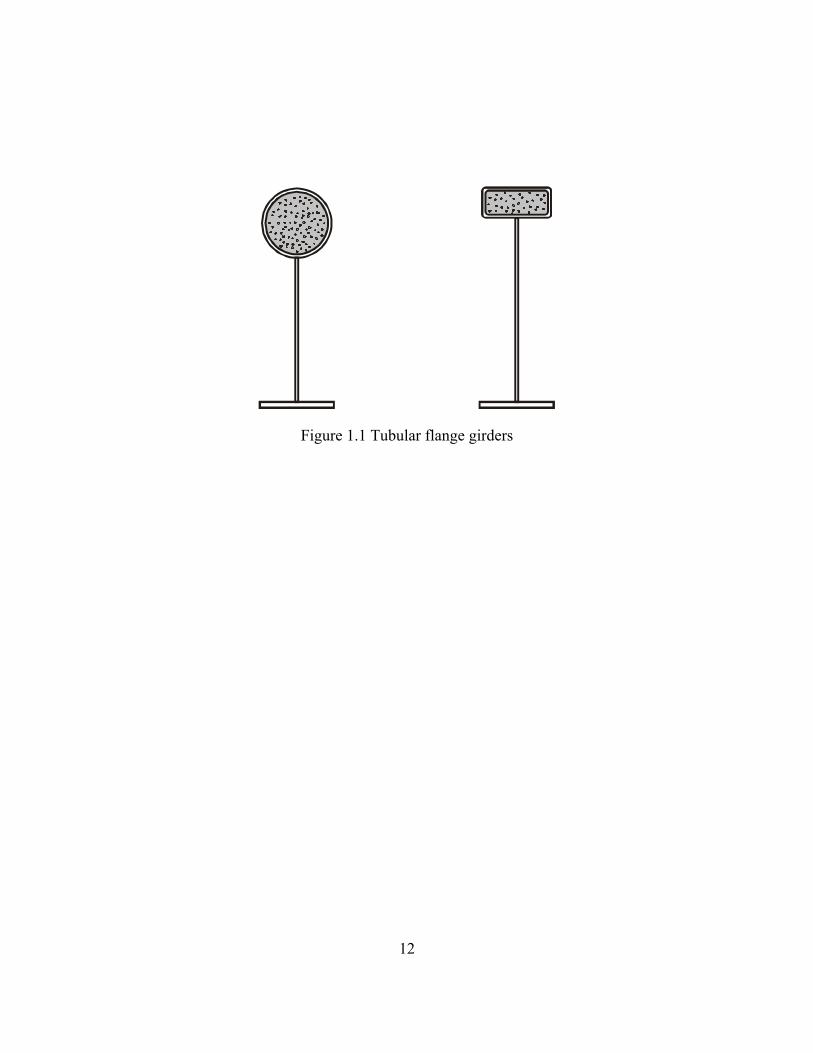
Figure 1.1 Tubular flange girders.............................................................................12
Figure 2.1 Comparison of stress distribution based on actual response, simple plastic
theory, and strain compatibility for composite compact-section flexural
strength when PNA is in deck.................................................................33
Figure 2.2 Comparison of stress distribution based on actual response, simple plastic
theory, and strain compatibility for composite compact-section flexural
strength when PNA is in girder...............................................................33
Figure 2.3 Transformed section for CFTFG ............................................................33
Figure 2.4 Yield moment based on strain compatibility ..........................................34
Figure 2.5 Comparison of stress distribution based on actual response, simple plastic
theory, and strain compatibility for non-composite compact-section flexural
strength....................................................................................................34
Figure 2.6 Flexural stress for composite CFTFG under Service II loading conditions
(transformed section approach) ..............................................................34
Figure 2.7 Flexural stress for composite CFTFG under Service II loading conditions
(equivalent rectangular stress block approach).......................................35
Figure 2.8 Flexural stress for composite CFTFG under Fatigue loading conditions35
Figure 2.9 Flexural stress for non-composite CFTFG under Service II loading
conditions (transformed section approach).............................................35
Figure 2.10 Flexural stress for non-composite CFTFG under Service II loading
conditions (equivalent rectangular stress block approach) .....................36
Figure 2.11 Flexural stress for non-composite CFTFG under Fatigue loading
conditions................................................................................................36
Figure 3.1 Demonstration bridge cross-section........................................................51
Figure 3.2 Option 1 for construction sequence of bridge (Construction Option 1) .52
Figure 3.3 Option 2 for construction sequence of bridge (Construction Option 2) .53
Figure 3.4 Unfactored dead and live load moment envelopes for Construction
Option 1 ..................................................................................................54

8
Figure 3.5 Unfactored dead and live load shear envelopes for Construction
Option 1 ..................................................................................................54
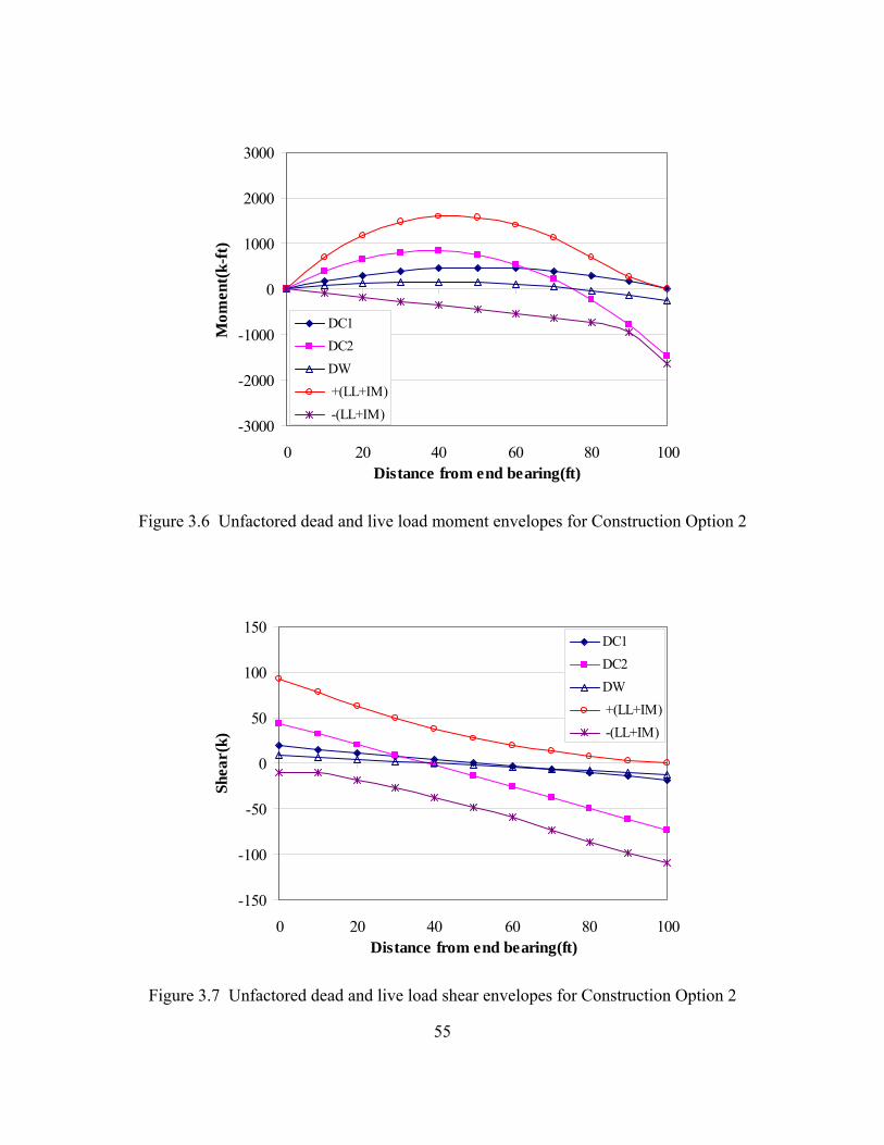
Figure 3.6 Unfactored dead and live load moment envelopes for Construction
Option 2 ..................................................................................................55
Figure 3.7 Unfactored dead and live load shear envelopes for Construction
Option 2 ..................................................................................................55
Figure 3.8 Section considered for pier section design .............................................56
Figure 3.9 Factored moment envelopes due to Strength I loading for Construction
Option 1 ..................................................................................................56
Figure 3.10 Girders of demonstration bridge .............................................................57
Figure 3.11 Field splice design .................................................................................58
Figure 4.1 General overview of precast concrete deck system ................................65
Figure 4.2 Schematic drawings of precast concrete deck panels .............................66
Figure 4.3 Schematic drawings of precast concrete deck panels including pockets67
Figure 5.1 Design flexural strength for construction loading conditions.................78

9
CHAPTER 1 INTRODUCTION
1.1 OVERVIEW
The tubular flange girder system is one of several innovative steel bridge girder
systems proposed by Wassef et al. (1997) and Sause and Fisher (1996) over the past
several years. Research funded by the Federal Highway Administration (Wimer and
Sause 2004, and Kim and Sause 2005) has taken tubular flange girders from concept to
laboratory prototype (Figure 1.1). This research has established fundamental information
on the behavior of these girders under simulated bridge loading conditions. The concrete-
filled tubular flange girders (CFTFGs) shown in Figure 1.1 have several advantages
compared to conventional I-girders (Kim and Sause 2005). Two main advantages are: (1)
the concrete-filled tubular flange provides more strength, stiffness, and lateral torsional
stability than a flat plate flange with the same amount of steel, and (2) the vertical
dimension of the tube reduces the web depth, thereby reducing the web slenderness. In
particular, the increased torsional stability of the girders will reduced the number of
diaphragms (or cross-frames) needed to brace the girders, thus reducing the time and cost
of fabricating and erecting the bridge girder system.
This report presents a design study of a tubular flange girder demonstration bridge,
conducted for the Pennsylvania Department of Transportation (PENNDOT). The bridge
girders are CFTFGs comprised of a conventional web plate and bottom flange plate, and
a top flange fabricated from a rectangular tube that is then filled with concrete.
The CFTFGs are designed to be constructed as simple spans for dead loads, and are
then made continuous for superimposed dead loads and live loads by adding continuity at
10
the pier. This construction sequence reduces the loads carried by the continuous girders
so that the design moments and shears for the interior-pier sections of the girders and for
the field splices at the pier are reduced. Also, to promote accelerated construction, the
bridge is designed to be constructed with precast deck panels.
1.2 COMPLETED TASKS
The study included the following completed tasks:
(1) Develop Design Criteria
Based on the results of previous research on CFTFGs, CFTFG design criteria were
developed in a format (i.e., LRFD format) compatible with the 2000 PENNDOT Design
Manual Part 4 (PENNDOT 2000) and the 2004 AASHTO LRFD Bridge Design
Specifications (AASHTO 2004). This task considered the main loading conditions
considered in bridge design (maximum load, overload, fatigue, etc.) and particularly
emphasized construction conditions, where CFTFGs provide their greatest benefits.
(2) Preliminary Design of CFTFGs for Demonstration Bridge
A preliminary design of the CFTFGs for the demonstration bridge was developed.
The bridge is a two-span bridge, designed to be constructed as simple spans for dead load,
which are made continuous for superimposed dead loads and live loads by adding
continuity at the pier. The preliminary design was developed for spans of 100 ft.
Preliminary dimensions of the CFTFGs were developed. The process of selecting these
dimensions illustrates the application of the design criteria. The resulting girder
dimensions were used in the remaining tasks, and will provide a starting point for
engineers responsible for the design of the demonstration bridge.

11
(3) Preliminary Design of Field Splice
The demonstration bridge is a two-span bridge, which requires a field splice that is
located at the pier. A preliminary design of the splice was developed. This design
provides a starting point for engineers responsible for the design of the demonstration
bridge.
(4) Preliminary Design of Precast Concrete Deck
A preliminary design for a precast concrete deck for the demonstration bridge was
developed.
(5) Finite Element Analyses
Based on CFTFG stability analyses conducted by previous research, finite element
analyses of the stability of the demonstration bridge girders under critical construction
loading conditions were conducted. These analyses validated the design criteria, and
provide information for the engineers responsible for the design of the demonstration
bridge.
12
Figure 1.1 Tubular flange girders

13
CHAPTER 2 DESIGN CRITERIA FOR TUBULAR FLANGE
BRIDGE GIRDERS
2.1 INTRODUCTION
Design criteria for concrete-filled tubular flange girders (CFTFGs) recommended
herein were developed from the results of an analytical and experimental investigation
conducted by Kim and Sause (2005). This investigation studied CFTFGs with steel yield
strengths of 70 ksi and 100 ksi. The design criteria are considered applicable for
CFTFGs with yield strength ranging from 50 ksi to 100 ksi.
2.2 GENERAL
Design criteria presented here apply to flexure of straight CFTFGs that are
symmetrical about a vertical axis in the plane of the web. These criteria cover the
following types of CFTFGs.
• CFTFGs that are composite with a concrete deck in positive flexure, where the
concrete-filled tubular flange is the top (compression) flange.
• CFTFGs that are non-composite with a concrete deck in positive or negative flexure,
where the concrete-filled tubular flange is the compression flange.
When the CFTFG is loaded in positive or negative flexure so that the concrete-filled
tubular flange is the tension flange, then the concrete in the steel tube is neglected, and
the CFTFGs can be designed based on the 2004 AASHTO LRFD Bridge Design
Specifications (AASHTO 2004).
The design criteria presented here are compatible with the 2004 AASHTO LRFD
14
specifications (AASHTO 2004). Criteria are given for the design of CFTFGs for the
following requirements. Other requirements may need to be considered.
• The Strength I limit state requirements.
• The Constructibility requirements.
• The Service II limit state requirements.
• The Fatigue limit state requirements.
Strength I limit state requirements ensure that strength and stability, both local and
global, are provided to resist the set of loading conditions that represents the maximum
loading under normal use of the bridge. Constructibility requirements ensure that
adequate strength is provided to resist the set of loading conditions that develop during
critical stages of construction, but under which nominal yielding or reliance on post-
buckling resistance is not permitted. Service II limit state requirements restrict yielding
and permanent deformation of the steel structure under the set of loading conditions that
represent normal service conditions. Fatigue limit state requirements restrict the stress
range due to the passage of the fatigue design truck.
2.3 CFTFGS COMPOSITE WITH CONCRETE DECK
Sections consisting of a CFTFG section connected with sufficient shear connectors
to a concrete deck to provide composite action and lateral support are considered
composite sections.
15
2.3.1 Strength I Limit State
Flexural Strength
Composite sections are designed as compact sections by satisfying the following
conditions:
• Compact section web slenderness limit:
ycweb
cp
FE76.3
TD
2 ≤ (2.1)
• Tube local buckling requirement:
yctube
tube
FE7.1
TB
≤ (2.2)
where, cpD is the depth of the web in compression at the composite compact section
moment, scccM ,which is given below, webT is the web thickness, E is the elastic modulus
of the steel, ycF is the yield stress of the compression flange (tube steel), Btube is the tube
width, and Ttube is the tube thickness. Equation (2.2) is adopted from Article 6.9.4 of the
2004 AASHTO LRFD specifications (AASHTO 2004). It allows the tubular flange to
yield before buckling locally in compression, and is conservative for a concrete-filled
tube. Equations (2.1) and (2.2) replace Equation 6.10.6.2.2-1 from Article 6.10.6.2.2 and
Equations 6.10.2.2-1 and 6.10.2.2-3 from Article 6.10.2.2 of the 2004 AASHTO LRFD
specifications (AASHTO 2004).
The design criterion for flexure of composite CFTFGs for the Strength I limit state
is as follows:
nfu MM φ≤ (2.3)
16
where, uM is the largest value of the major-axis bending moment in the girder due to the
factored loads as specified in Chapter 3 of the 2004 AASHTO LRFD specifications
(AASHTO 2004), fφ is the resistance factor for flexure, taken as 1.0 in the 2004
AASHTO LRFD specifications (AASHTO 2004), and nM is the nominal flexural
strength. Equation (2.3) replaces Equation 6.10.7.1.1-1 from Article 6.10.7.1.1 of the
2004 AASHTO LRFD specifications (AASHTO 2004).
The nominal flexural strength is taken as:
scccn MM = (2.4)
scccM is determined using an equivalent rectangular stress block for the concrete and an
elastic perfectly plastic stress-strain curve for the steel. The maximum usable strain at the
extreme concrete compression fiber, which is at the top of the deck, is taken as 0.003.
Note that for the calculation of scccM , the concrete in the haunch is ignored. Figures 2.1
and 2.2 compare stress distributions based on the actual response, simple plastic theory,
and strain compatibility for composite compact-section CFTFGs at the positive flexural
strength limit, when the plastic neutral axis (PNA) is located in the deck and girder,
respectively. β1 shown in these figures is based on the compressive strength (fc') of the
concrete deck. If fc' is less than or equal to 4 ksi, then β1 is 0.85, and β1 is reduced
continuously by 0.05 for each 1 ksi of strength in excess of 4 ksi. These figures indicate
that the strain compatibility approach reasonably approximates the actual stress
distribution regardless of the PNA location and steel grade, and thus the method should
accurately estimate the flexural strength. Equation (2.4) generally replaces the nominal
flexural resistance calculations of Article 6.10.7.1.2 of the 2004 AASHTO LRFD

17
specifications (AASHTO 2004), although the limit on nM given by Equation 6.10.7.1.2-
3 from Article 6.10.7.1.2 should be applied.
Shear Strength
The design criterion for shear of composite CFTFGs for the Strength I limit state is
as follows:
nvu VV φ≤ (2.5)
where, uV is the shear in the web at the section under consideration due to the factored
loads as specified in the 2004 AASHTO LRFD specifications (AASHTO 2004), vφ is
the resistance factor for shear, taken as 1.0 in the 2004 AASHTO LRFD specifications
(AASHTO 2004), and nV is the nominal shear strength determined as specified in Article
6.10.9.2 of the 2004 AASHTO LRFD specifications (AASHTO 2004) without
modification. Note that Equation (2.5) simply restates Equation 6.10.9.1-1 from Article
6.10.9.1 of the 2004 AASHTO LRFD specifications (AASHTO 2004). All of the vertical
shear force is assumed to be carried by the web.
2.3.2 Constructibility
The design criteria presented here pertain to conditions before the CFTFG is made
composite with the concrete deck. These criteria apply only when the following
conditions are satisfied:
• Web slenderness limit for “stocky web” under flexure:

18
ycb
web
c
FE
T2D
λ≤ (2.6)
• Web slenderness limit to minimize web distortion:
31
yctweb
web
FE11
TD
⎟⎟⎠
⎞⎜⎜⎝
⎛≤ (2.7)
• The tube local buckling requirement given by Equation (2.2) is satisfied.
• Transverse stiffeners are provided at three (or more) equally-spaced locations along
the span (i.e., quarter-span, mid-span, and three quarter-span) plus the bearing
locations (more details are presented below).
In Equations (2.6) and (2.7), cD is the depth of the web in compression at the yield
moment ( yM ) for the CFTFG when it is non-composite with the concrete deck, bλ is a
coefficient related to the boundary conditions provided to the web by the flanges, webD is
the web depth, and yctF is the smaller of the yield stress for the compression flange and
the yield stress for the tension flange. Equation (2.6) replaces Equation 6.10.3.2.1-3 from
Article 6.10.3.2.1 of the 2004 AASHTO LRFD specifications (AASHTO 2004).
If the area of the compression flange (the area of the steel tube plus the transformed
area of the concrete infill) is less than that of tension flange, the value of bλ is 4.64,
otherwise, the value of bλ is 5.76 as given in Article 6.10.4.3.2 of the 1998 AASHTO
LRFD specifications (AASHTO 1998).
The web slenderness requirement given by Equation (2.7) is based on finite element
analysis results for CFTFGs with a stiffener arrangement having three intermediate
stiffeners equally spaced along the span and stiffeners at each bearing. The details behind

19
this equation are discussed in Kim and Sause (2005).
The arrangement of three intermediate transverse stiffeners along the span, suggested
here, minimizes the effect of section distortion on the LTB strength without requiring too
many stiffeners. The stiffeners should be placed in pairs, one on each side of the web, and
the stiffeners should be spaced equally along the span. The following suggestions are
made:
• The bearing and intermediate transverse stiffeners are made identical to simplify
fabrication.
• The total width of each pair of stiffeners, including the web thickness, is 95% of the
smaller of the tube width and the bottom flange width.
• The yield stress of the stiffeners is equal to yield stress of the steel elements of the
girder cross-section.
The design criterion for flexure of composite CFTFGs for Constructibility is
nfu MM φ≤ , which is identical in form to Equation (2.3). Again, uM is the largest value
of the major-axis bending moment in the girder due to factored loads specified in
Chapter 3 of the 2004 AASHTO LRFD specifications (AASHTO 2004). Here, Equation
(2.3) is used in place of Equations 6.10.3.2.1-1 and 6.10.3.2.1-2 from Article 6.10.3.2.1
and Equation 6.10.3.2.2-1 from Article 6.10.3.2.2, and the calculation of nM (given
below) replaces the calculation of ycF , ncF , and ytF for a noncomposite section from
Article 6.10.3.2.1 and Article 6.10.3.2.2, which refer to Article 6.10.8 of the 2004
AASHTO LRFD specifications (AASHTO 2004).
The nominal flexural strength, nM , is taken as:
20
)MandM(MM dsbrdn ≤= (2.8)
where, brdM is the design flexural strength for torsionally braced CFTFGs, sM is the
cross-section flexural capacity which can be taken as the yield moment, yM , when the
steel tube yield stress is 70 ksi or less, and dM is an ideal design flexural strength that
corresponds to buckling between the brace points (assuming each diaphragm provides
perfect lateral and torsional bracing at the brace point). Note that if the tube yield stress is
large (e.g., 100 ksi) and the compressive strength of the concrete infill is small (e.g., 4
ksi), then the non-composite compact section moment capacity, scnccM , may be less than
yM . In this case, scnccM should be calculated and used for sM (Kim and Sause 2005).
yM for a CFTFG non-composite with the concrete deck is taken as the smaller of the
yield moment based on analysis of a linear elastic transformed section, tryM , and the yield
moment based on strain compatibility, scyM , which uses an equivalent stress block for
concrete in the tube. yM is also the smaller of the yield moment with respect to the
compression flange, ycM , and the yield moment with respect to the tension flange, ytM .
In calculating tryM , the concrete in the steel tube is transformed to an equivalent area of
steel using the modular ratio as shown in Figure 2.3 (cE
En = , where, cE is the elastic
modulus of concrete). scyM is calculated based on an equivalent rectangular stress block
for the concrete in the steel tube and a linear elastic stress-strain curve for the steel with
the yield strain, yε , reached at either the top or bottom fiber. Note that for the calculation
21
of scyM , the strain in the concrete in the steel tube is not calculated, because the strain is
limited to the yield strain of the tube. Figure 2.4 shows scyM when either the top
(compression) or the bottom (tension) flange yields first. A suggestion, that must be used
with care, is that when the ratio of the yield stress of the tube steel, ytubeF , to the
compressive strength of the concrete infill, fc', is smaller than 8.5, yM is taken as tryM .
Otherwise, yM is taken as scyM .
scnccM is the flexural strength based on strain compatibility, and is determined using
an equivalent rectangular stress block for the concrete and an elastic perfectly plastic
stress-strain curve for the steel as shown in Figure 2.5. The maximum usable strain is
assumed to be 0.003 at the top of the concrete in the steel tube. The stress distributions
based on the actual response, simple plastic theory, and strain compatibility for non-
composite compact-section CFTFGs at the positive flexural limit state are shown in
Figure 2.5.
The ideal design flexural strength is given by
sssbd MMCM ≤α= (2.9)
where, bC is the moment gradient correction factor and sα is the strength reduction
factor. The moment gradient correction factor is given by either
CBAmax
maxb M3M4M3M5.2
M5.12C
+++= (2.10a)
or
3.2MM3.0
MM05.175.1C
2
2
1
2
1b ≤⎟⎟
⎠
⎞⎜⎜⎝
⎛+⎟⎟
⎠
⎞⎜⎜⎝
⎛−= (2.10b)
22
where in Equation (2.10a), maxM is the absolute value of the maximum moment in the
unbraced segment and AM , BM , and CM are the absolute values of the moment at the
quarter, center, and three-quarter points in the unbraced segment, respectively. In
Equation (2.10b), 1M is the moment at the bracing point opposite to the one
corresponding to 2M , and is taken as positive when it causes compression and negative
when it causes tension in the flange under consideration. 2M is the largest major-axis
bending moment at either end of the unbraced length causing compression in the flange
under consideration, and is taken as positive. Equation (2.10a) provides more accurate
results for cases with non-linear moment diagrams, and has been used in calculations
made for the preliminary design of the CFTFGs for the demonstration bridge discussed in
Chapter 3. Equation (2.10a) was given in the commentary of past editions of the
AASHTO LRFD specifications, but is not in the 2004 AASHTO LRFD specifications
(AASHTO 2004), which provide specific guidance on definition of 1M and 2M for non-
linear moment diagrams to make the results from Equation (2.10b) conservative.
The strength reduction factor is given by
0.1MM
2.2MM
8.0cr
s
2
cr
ss ≤
⎟⎟⎟
⎠
⎞
⎜⎜⎜
⎝
⎛−+⎟⎟
⎠
⎞⎜⎜⎝
⎛=α (2.11)
where, crM is the elastic LTB moment, given by
( )2yb
2tr
2
trTyb
cr rLAd
467.2AK385.0rL
EM +π
= (2.12)
where, E is the elastic modulus of steel, bL is the unbraced length, yr is the radius of

23
gyration, TK is the St. Venant torsional inertia of the transformed section (using the
short-term modular ratio), trA is the transformed section area (using the short-term
modular ratio), and d is the section depth. The radius of gyration is given by
tr
bftfy A
IIr
+= (2.13)
where, tfI and bfI are the moments of inertia of the top and bottom flanges about the
vertical axis, respectively. Note that tfI is based on a transformed section for the
concrete-filled steel tube using the short-term modular ratio to account for the concrete in
the tube.
For Equation (2.8), the design flexural strength for torsionally braced CFTFGs, brdM ,
is considered because research (Kim and Sause 2005) shows that the bracing provided to
a CFTFG by a typical system of interior diaphragms may not be sufficiently stiff to brace
the CFTFGs so that lateral buckling occurs only between the brace points. The approach
taken here is given by Kim and Sause (2005) and is based on the approach described by
Yura et al. (1992). brdM is given by
sbrsbu
brd MCM α= (2.14)
where, buC is the moment gradient correction factor corresponding to the girder when it
is braced only at the ends of the span (without interior bracing within the span), obtained
by applying Equation (2.10) to the entire girder span and brsα is a strength reduction
factor for the torsionally braced girder. The strength reduction factor for the torsionally
braced girder is given by
24
0.1MM
2.2MM
8.0 brcr
s
2
brcr
sbrs ≤
⎟⎟⎟
⎠
⎞
⎜⎜⎜
⎝
⎛−+⎟⎟
⎠
⎞⎜⎜⎝
⎛=α (2.15)
where, brcrM is the elastic LTB moment including the torsional brace stiffness, which is
based on the approach described by Yura et al. (1992), and given by
2br2
bu
2bb2ubr
crbrcr M
CC
MM += (2.16)
where, ubrcrM is the elastic LTB moment for the girder without interior bracing within the
span, bbC is the moment gradient correction factor corresponding to the unbraced
segment under investigation, assuming the adjacent brace points provide perfect bracing,
obtained by applying Equation (2.10) to the unbraced segment, and brM is the moment
including the torsional bracing effect, given later. ubrcrM is given by
( )2y
2tr
2
trTy
ubrcr rL
Ad467.2AK385.0
rLEM +
π= (2.17)
Note that Equation (2.17) is Equation (2.12) with bL replaced by the span length L . The
moment including the torsional bracing effect, brM , which is derived by Yura et al.
(1992), is given by
L2.1nIE
M effTbr
β= (2.18)
where, Tβ is the effective brace stiffness, effI is the effective vertical axis moment of
inertia of the girder to account for singly-symmetric sections, and n is the number of
interior braces within the span. The effective brace stiffness is given by (Yura et al. 1992)

25
gsecbT
1111β
+β
+β
=β
(2.19)
where, bβ is the discrete brace stiffness, secβ is the stiffness of the web and stiffeners,
and gβ is the stiffness of the girder system. bβ , gβ , and secβ have dimensions of force-
length. For multi-girder systems connected with diaphragms, they can be calculated from
the following equations (Yura et al. 1992).
SIE6 b
b =β (2.20)
3x
2
g
2g
g LIES
n)1n(24 −
=β (2.21)
( )⎟⎟⎠
⎞⎜⎜⎝
⎛+
+=β
12bt
12th5.1N
hE3.3
3ss
3w
sec (2.22)
In Equations (2.20) to (2.22), S is the spacing of girders, bI is the moment of inertia of
the bracing member about the strong axis, xI is the horizontal axis moment of inertia of
the girder, gn is the number of girders, h is the distance between flange centroids, N is
the contact length of the torsional brace, wt is the web thickness, st is the stiffener
thickness, and sb is the stiffener width. N can be taken as the thickness of the
diaphragm connection plate. The effective vertical axis moment of inertia of the girder is
given by
ytyceff IctII += (2.23)
where, ycI and ytI are the vertical axis moment of inertia of the compression and tension
flanges respectively, and c and t are the distances from the neutral axis to the centroid of

26
the compression and tension flanges respectively.
2.3.3 Service II Limit State
The design criterion for composite CFTFGs for the Service II limit state is as
follows:
yfhf FR95.0f ≤ (2.24)
where, ff is the flexural stress in the flanges caused by the factored loads as specified in
Chapter 3 of the 2004 AASHTO LRFD specifications (AASHTO 2004), hR is the
hybrid factor, and yfF is the yield stress of the flange. Note that hR accounts for the
nonlinear variation of stresses caused by yielding of the lower strength steel in the web of
a hybrid girder (a coefficient ≤ 1.0) as specified in Article 6.10.1.10.1 of the 2004
AASHTO LRFD specifications (AASHTO 2004).
Equation (2.24) replaces Equations 6.10.4.2.2-1 and 6.10.4.2.2-2 from Article
6.10.4.2.2 of the 2004 AASHTO LRFD specifications (AASHTO 2004). Equations (2.1),
(2.6), and (2.7) are intended to prohibit the use of slender webs in CFTFGs. For
CFTFGS that are composite with the concrete deck and under positive flexure, no further
check on web slenderness is needed, and Equation 6.10.4.2.2-4 from Article 6.10.4.2.2 of
the 2004 AASHTO LRFD specifications (AASHTO 2004) is not considered. However,
for CFTFGs that are composite with a concrete deck under negative flexure with the
concrete-filled tubular flange as the compression (bottom) flange (a condition that is not
covered by the design criteria presented in this chapter), Equation 6.10.4.2.2-4 from
Article 6.10.4.2.2 of the 2004 AASHTO LRFD specifications (AASHTO 2004) should

27
be considered.
Two different approaches are used to include the concrete in the steel tube in the
calculation of the flexural stress. The first approach uses a transformed section to include
the concrete in the tube, and the second approach uses an equivalent rectangular stress
block for the concrete.
When scy
try MM ≤ , then the transformed section approach is used for the concrete in
the steel tube, and the flexural stresses are calculated as the sum of the stresses due to
following individual loading conditions (Figure 2.6):
• The factored DC moment acting on the non-composite section, where the long-term
modular ratio is used to account for the concrete in the steel tube (which makes a
significant contribution to the stiffness and strength of the non-composite section).
• The factored DW moment acting on the long-term composite section, including the
concrete deck but neglecting the concrete in the steel tube (which makes a negligible
contribution to the stiffness and strength of the composite section).
• The factored LL moment acting on the short-term composite section, including the
concrete deck but neglecting the concrete in the steel tube.
When scy
try MM > , then the equivalent rectangular stress block approach is used for
the concrete in the steel tube, and the flexural stresses are calculated as the sum of the
stresses due to following individual loading conditions (Figure 2.7):
• The factored DC moment acting on the non-composite section, where the equivalent
rectangular stress block is used to account for the concrete in the steel tube.
• The factored DW moment acting on the long-term composite section, including the

28
concrete deck but neglecting the concrete in the steel tube.
• The factored LL moment acting on the short-term composite section, including the
concrete deck but neglecting the concrete in the steel tube.
The long-term composite section is a transformed section based on an increased
modular ratio (i.e., the long-term modular ratio equal to 3n) to account for the creep of
the concrete that will occur over time. The short-term composite section is a transformed
section based on the usual modular ratio (i.e., the short-term modular ratio equal to n).
2.3.4 Fatigue Limit State
The design criterion for composite CFTFGs for the Fatigue limit state is as follows:
( ) ( )nFf Δ≤Δγ (2.25)
where, γ is the load factor and fΔ is the stress range due to the fatigue load as specified
in Chapter 3 of the 2004 AASHTO LRFD specifications (AASHTO 2004). ( )nFΔ is the
nominal fatigue resistance as specified in Article 6.6.1.2.5 of the 2004 AASHTO LRFD
specifications (AASHTO 2004). Equation (2.25) is a restatement of Equation 6.6.1.2.2-1
from Article 6.6.1.2.2 of the 2004 AASHTO LRFD specifications (AASHTO 2004).
fΔ is calculated using the transformed section approach. The concrete in the steel
tube and concrete deck are transformed to an equivalent area of steel using the short-term
composite section (Figure 2.8). The provisions of Article 6.10.5.3.1 of the 2004
AASHTO LRFD specifications (AASHTO 2004) should be considered, but are unlikely
to control for CFTFGs with stocky webs.
29
2.4 CFTFGS NON-COMPOSITE WITH CONCRETE DECK
Sections consisting of a CFTFG that is not connected to the concrete deck by shear
connectors are considered non-composite sections.
2.4.1 Strength I Limit State
Flexural Strength
Non-composite sections are designed to be either compact sections or non-compact
sections by satisfying the following conditions:
• Compact sections satisfy the compact section web slenderness limit given by
Equation (2.1):
• Non-compact sections satisfy the non-compact section web slenderness limit given
by:
ycweb
c
FE7.5
TD
2 < (2.26)
• Compact sections and non-compact sections satisfy the tube local buckling
requirement given by Equation (2.2):
The design criterion for flexure of non-composite CFTFGs for the Strength I limit
state is expressed in the same form as Equation (2.3). In Equation (2.3), uM is, again, the
largest value of the major-axis bending moment within an unbraced length due to the
factored loads as specified in Chapter 3 of the 2004 AASHTO LRFD specifications
(AASHTO 2004). The nominal flexural strength, nM , is determined from Equation (2.8)
with small modifications. If the girders are laterally braced by the deck, it is assumed that
the attachments to the deck provide perfectly lateral and torsional bracing. Therefore, for
calculating brdM for Equation (2.8), the unbraced length (Lb) between attachments to the
30
deck is used instead of the span length (L) in Equations (2.17) and (2.18). If the deck
does not brace the girders, the span length (L) is used to calculate brdM for Equation (2.8).
In both cases, the cross-section flexural capacity, sM , is taken as
ycpcs MRM = (2.27)
where, pcR is the web plastification factor for the compression flange as specified in
Article A6.2 of the 2004 AASHTO LRFD specifications (AASHTO 2004), and ycM is
the yield moment with respect to the compression flange, described earlier in Section
2.3.2.
Shear Strength
The design recommendations for shear of non-composite CFTFGs for the Strength I
limit state are the same as those for composite CFTFGs given in Section 2.3.1.
2.4.2 Constructibility
Design recommendations for non-composite CFTFGs for Constructibility are the
same as those for composite CFTFGs given in Section 3.2.
2.4.3 Service II Limit State
The design criterion for non-composite CFTFGs for the Service II limit state is as
follows:
yfhf FR80.0f ≤ (2.28)
where, ff is the flexural stress in the flanges caused by the factored loads as

31
specified in Chapter 3 of the 2004 AASHTO LRFD specifications (AASHTO 2004), hR
is the hybrid factor, and yfF is the yield stress of the flange. Equation (2.28) replaces
Equations 6.10.4.2.2-3 from Article 6.10.4.2.2 of the 2004 AASHTO LRFD
specifications (AASHTO 2004). Equation 6.10.4.2.2-4 from Article 6.10.4.2.2 of the
2004 AASHTO LRFD specifications (AASHTO 2004) should be considered.
Similar to composite CFTFGs, two different approaches (i.e., the transformed
section approach and the equivalent rectangular stress block approach) are used to
include the concrete in the steel tube in the calculating the flexural stress.
When scy
try MM ≤ , then the transformed section approach is used for the concrete in
the steel tube, and the flexural stresses are calculated as the sum of the stresses due to
following individual loading conditions (Figure 2.9):
• The factored DC moment and DW moment acting on the non-composite section,
where the long-term composite section is used to account for the concrete in the
steel tube.
• The factored LL moment acting on the non-composite section, where the short-term
composite section is used to account for the concrete in the steel tube.
When scy
try MM > , then the equivalent rectangular stress block approach is used for
the concrete in the steel tube, and the flexural stresses are calculated as the sum of the
stresses due to following individual loading conditions (Figure 2.10):
• The factored DC, DW, and LL moments acting on the non-composite section, where
the equivalent rectangular stress block is used to account for the concrete in the steel
tube.
32
2.4.4 Fatigue Limit State
Design recommendations for non-composite CFTFGs for the Fatigue limit state are
the same as those for composite CFTFGs given in Section 3.4, except for the calculation
of fΔ . The calculation of fΔ is based on the short-term composite section, including
only the steel girder and the concrete in the steel tube (Figure 2.11).

33
PNA
0.003εy
εy
0.85fc’ 0.85fc’fc’
Fy Fy>Fy
C
T
Actual Response
Simple Plastic Theory
Strain Compatibility
c β1c
Figure 2.1 Comparison of stress distribution based on actual response, simple plastic theory, and strain compatibility for composite compact-section flexural strength when
PNA is in deck
PNAC
T
0.003
εy
εy
0.85fc’
Fy
Fy
Fy
0.85fc’fc’
Fy
Actual Response
Simple Plastic Theory
Strain Compatibility
c β1c
Figure 2.2 Comparison of stress distribution based on actual response, simple plastic theory, and strain compatibility for composite compact-section flexural strength when
PNA is in girder
dA dA/n
Figure 2.3 Transformed section for CFTFG

34
ENA
C
εy Fy
0.85fc’< εy < Fy
C
< εy < Fy
0.85fc’ εy Fy
TT
(b) When bottom (tension) flange yields first
(a) When top (compression) flange yields first
Figure 2.4 Yield moment based on strain compatibility
PNA
C
T
0.003
εy
εy
0.85fc’
Fy
Fy
Fy
0.85fc’fc’
Fy
Actual Response
Simple Plastic Theory
Strain Compatibility
FyFy
Figure 2.5 Comparison of stress distribution based on actual response, simple plastic theory, and strain compatibility for non-composite compact-section flexural strength
(a) Due to DC (b) Due to DW (c) Due to LL
Long-term Long-term Short-term
Figure 2.6 Flexural stress for composite CFTFG under Service II loading conditions (transformed section approach)

35
(a) Due to DC (b) Due to DW (c) Due to LL
Short-termLong-term
Figure 2.7 Flexural stress for composite CFTFG under Service II loading conditions (equivalent rectangular stress block approach)
Short-term
Figure 2.8 Flexural stress for composite CFTFG under Fatigue loading conditions
(a) Due to DC and DW (b) Due to LL
Long-term Short-term
Figure 2.9 Flexural stress for non-composite CFTFG under Service II loading conditions (transformed section approach)

36
Due to DC, DW, and LL
Figure 2.10 Flexural stress for non-composite CFTFG under Service II loading conditions (equivalent rectangular stress block approach)
Short-term
Figure 2.11 Flexural stress for non-composite CFTFG under Fatigue loading conditions

37
CHAPTER 3 PRELIMINARY DESIGN OF CFTFGS
FOR DEMONSTRATION BRIDGE
3.1 INTRODUCTION
A design study of a two-span continuous composite CFTFG demonstration bridge
with spans of 100 ft-100 ft is summarized here. This study developed a preliminary
flexural design of the critical positive moment section and the interior-pier section of the
CFTFGs for the demonstration bridge. The study also developed a preliminary design of
the field splice at the pier. The interior-pier section design and the field splice design
were actually completed after precast concrete deck design, presented in the next chapter,
was completed, but the design results are included in this chapter.
3.2 BRIDGE CROSS-SECTION
The demonstration bridge cross-section was provided by PENNDOT, and consists
of four girders spaced at 8 ft-5.5 in centers with 3 ft overhangs (Figure 3.1). The concrete
deck is 8 in. thick. ASTM A 709 Grade 50 steel and concrete with compressive strength
of 4 ksi were used. This design study considers the 2004 AASHTO LRFD Bridge Design
Specifications (AASHTO 2004) and the PENNDOT Design Manual Part 4 (PENNDOT
2000) as well as the design criteria given in Chapter 2. The design study results are based
on several assumptions: (1) end diaphragms, but no interior diaphragms within the spans
under construction conditions (during erection and deck placement) and one interior
diaphragm at mid-span under service conditions, (2) diaphragms are W21X57 steel
sections, (3) bearing stiffeners and three equally-spaced intermediate transverse stiffeners

38
(per span) with Category C′ fatigue details, (4) similar cross-sections for the positive
moment section and the pier section, and (5) a field splice located at the pier section.
3.3 GIRDER DESIGN
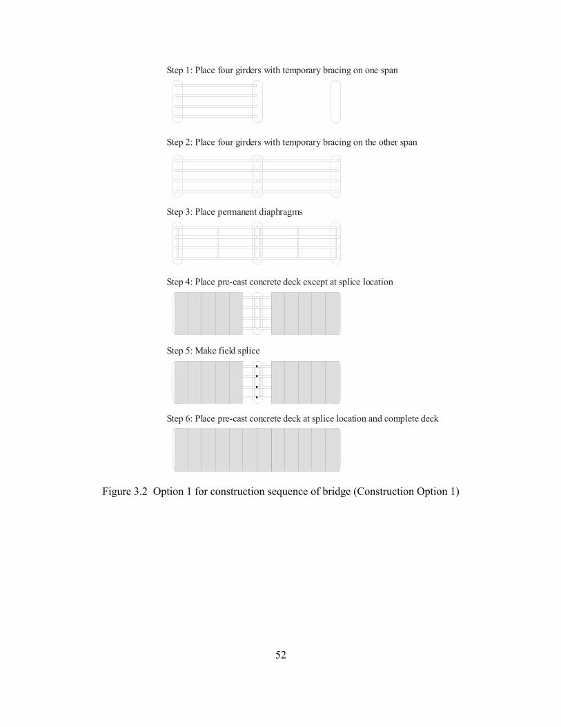
Two construction sequence options, shown in Figures 3.2 and 3.3, were considered
for the bridge. For Construction Option 1 (Figure 3.2), precast concrete deck panels are
placed on top of the girders except for the pier section where the field splice is located.
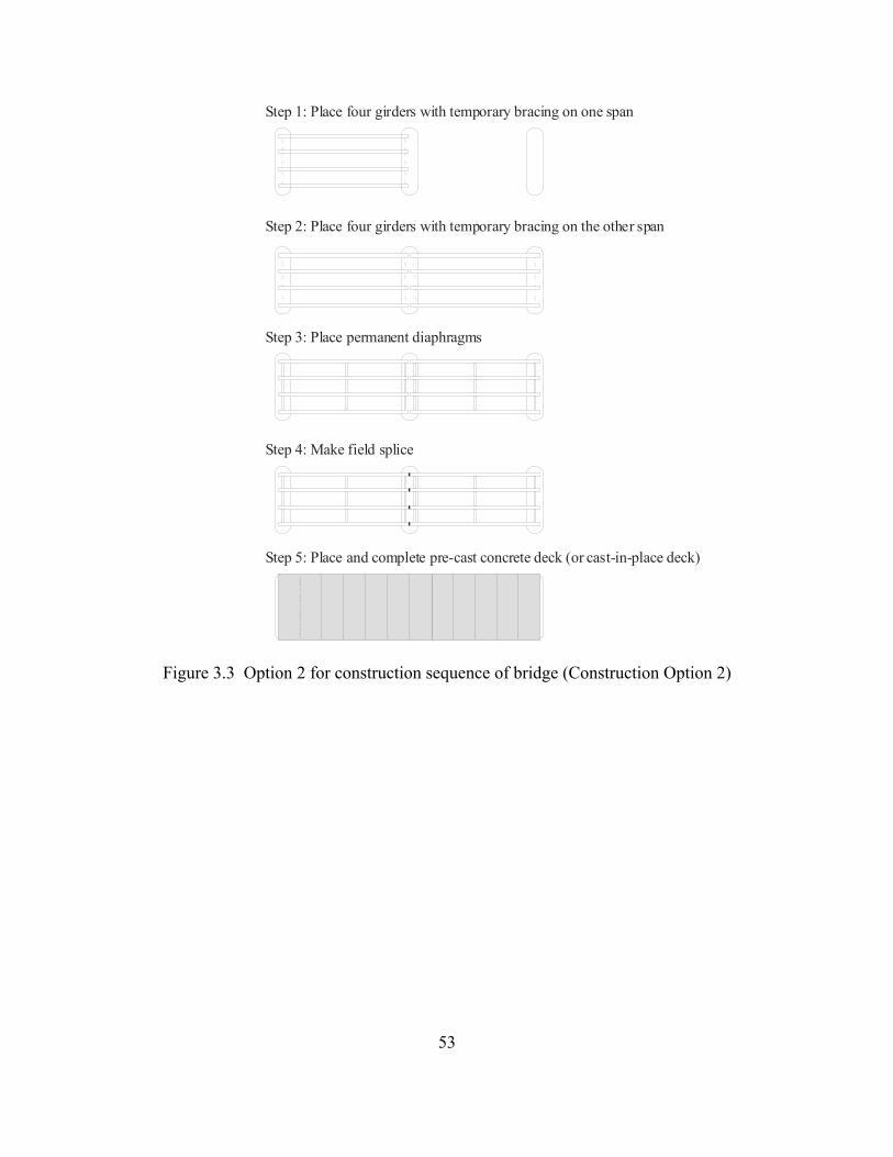
The field splice is then made and the final deck panel is placed. For Construction Option
2, the precast concrete deck panels are placed on top of the girders after the field splice is
made. Consequently, Construction Option 1 has less dead load applied to the continuous
span, which affects the design of the interior-pier section and the design of the field splice.
3.3.1 Design Loads
The girders were designed for various dead and live load conditions. Lateral loads
such as wind loads and earthquake loads were not considered in this study, however they
could be treated as they are in a conventional steel I-girder bridge.
The dead loads considered include the weight of all components of the structure, the
wearing surface, and the attached appurtenances. The dead load is divided into two
categories: (1) the weight of the bridge components and girders (Dc) and (2) the weight of
the future wearing surfaces (Dw). Dc includes the weight of the girders, the weight of the
deck, the weight of the haunch, the weight of the secondary steel (diaphragms, etc), and
the weight of the barriers. Dw includes the weight of the non-integral wearing surface. Dc
is also divided into two categories according to the time of field splice. Dc1 is Dc applied

39
to the simple spans and Dc2 is Dc applied to continuous spans. The dead loads were
computed as a weight per linear foot of bridge girder. The numerical values of these loads
are summarized in Table 3.1.
The live loads (LL) consist of either a design truck or design tandem acting
coincident with a uniformly distributed design lane load. The 2004 AASHTO LRFD
specifications (AASHTO 2004) specify the values and positions of these loads. The
design lane load is a 0.64 k/ft force distributed across a 10 ft design lane and over the
bridge such to cause the greatest load effect. In general, the live load analysis treats one
design truck or one design tandem on the bridge at a time, and this load is placed on the
bridge to cause the greatest load effect. Multiple presence factors account for loading in
more than one lane. Note that for the negative moment section at pier, as specified in the
2004 AASHTO LRFD specifications (AASHTO 2004), 90% of the effect of two design
trucks spaced a minimum of 50 ft between the lead axle of one truck and the rear axle of
the other truck was considered (along with 90% of the design lane load).
The design truck is an HS-20 truck, based on the 2004 AASHTO LRFD
specifications (AASHTO 2004) and the 2000 PENNDOT Design Manual Part 4
(PENNDOT 2000). The HS-20 truck includes three axle loads, the first is 8 kips, and the
second and the third are 32 kips. There is 14 ft between the first and second axle and 14
to 30 ft between the second and the third axle. The distance between the second and third
axle is varied to cause the greatest load effect on each girder.
The tandem load is a military loading which consists of a pair of 31.25 kip axles
spaced 4 ft apart (PENNDOT 2000). These loads are 125% of the AASHTO LRFD
design tandem (AASHTO 2004).

40
The fatigue load is based on an HS-20 truck with the axle spacing fixed at 14 ft
between the first and second axle and 30 ft between the second and the third axle. The
fatigue load consists of one such truck placed where it causes the greatest load effect. The
design lane load is not included in the fatigue load.
The live loads are increased by a dynamic load allowance to account for the
dynamic response. For most load cases, the effects of the design truck or tandem are
increased by 33% (AASHTO 2004). The dynamic load allowance is 15% for the fatigue
load effects. The lane load is not increased by the dynamic load allowance.
The live loads are given as lane loads and are not directly applied to each girder.
The loads are transmitted though the deck to the girders, and then to the supporting
substructure. Article 4.6.2.2 of the 2004 AASHTO LRFD specifications (AASHTO
2004) has live load distribution provisions to distribute the lane loads to the girders.
Distribution factors are applied to the live loads to determine the load applied to a girder,
and these distributed loads are used in calculating the girder moment and shear demands.
The distribution factors are calculated by using formulas in the specifications or by the
lever rule. The distribution factor formulas depend on the type of deck and the spacing
between the girders. In the lever rule, the fraction of live load distributed to each girder is
calculated by placing the loads on the bridge and summing moments about the adjacent
girder line. In addition, Article 4.6.2.2.2d of the 2004 AASHTO LRFD specifications
(AASHTO 2004) requires an additional distribution factor calculation which distributes
loads to an exterior girder by an analysis that treats the bridge cross-section as a rigid
cross-section that deflects and rotates as a rigid body under live loads (called the “rigid
body rule” distribution factor).

41
For interior girders, the specification formulas for a steel girder bridge with
concrete deck were used to calculate the distribution factors for shear and moment for the
girders of the demonstration bridge. For exterior girders, the lever rule was used with one
design lane loaded, the specification formulas were used with two or more design lanes
loaded to calculate the distribution factors for shear and moment. For the exterior girders,
the rigid body rule was also applied to both the one lane-loaded and the two or more lane-
loaded cases to calculate distribution factors for moment, and these distribution factors
controlled.
Tables 3.2 and 3.3 show the live load distribution factors for the non-fatigue limit
states and the Fatigue limit state, respectively. The interior and exterior girders of the
demonstration bridge were designed for same shear and moment, using the largest
distribution factors from those given in Tables 3.2 and 3.3. These distribution factors
were applied for both the positive and negative bending regions of the girders.
Figures 3.4, 3.5, 3.6, and 3.7 summarize the unfactored dead and live load girder
moment envelopes and shear envelopes for Construction Option 1 and Construction
Option 2. As shown in these figures, the girder dead and live load analyses generated
results at 10 ft intervals along the girder length. The figures show that the envelopes for
live load (LL) plus dynamic load allowance (IM) and for dead load due to the wearing
surface (Dw) are the same for Construction Option 1 and Construction Option 2. The
envelopes for dead load due to Dc1 and Dc2 vary for the different options. More Dc1 is
applied for Construction Option 1 than for Construction Option 2, but less Dc2 is applied
for Construction Option 1 than for Construction Option 2. As shown in Figures 3.4 and
3.6, Construction Option 1 has smaller negative moment at interior-pier section and field

42
splice location than Construction Option 2. Therefore, the design study was conducted
based on Construction Option 1.
With Construction Option 1 selected and the construction sequence more clear, the
dead load (Dc) can be further refined as follows. Dead load is applied to girders that may
be either simple-span or continuous and either non-composite with the deck or composite
with the deck. Dead load Dc1, as defined earlier, is applied to simple-span non-composite
girders, and includes the weight of the girders, the weight of the deck, and the weight of
the secondary steel (diaphragms, etc). Dead load Dc2, as defined earlier, is applied to
either non-composite or composite girders. Specifically, the weight of the haunch
(defined as Dc2a) is applied to girders that are continuous, but non-composite with the
deck, and the weight of the barriers (defined as Dc2b) is applied to girders that are
continuous and composite with the deck. Dw is also applied to girders that are continuous
and composite with the deck.
To simplify the preliminary design of the CFTFGs for the demonstration bridge
these various dead loads were treated as follows:
• To design the positive moment section, Dc1 and Dc2a are treated as Dc dead loads
applied to non-composite girders. When Dc1 is applied to the simple-span girders,
the maximum positive moment is at midspan. When the remaining loads are applied
to the continuous girders, the maximum positive moment is 40 ft from the abutment
end of the girders. For simplicity, these maximum positive moments were treated as
if they acted at the same cross section. More accurate design calculations would
treat these two cross sections independently.
• To design the negative moment region and splice at the pier, Dc1 which is applied to

43
the simple-span girders is omitted. Dc2a and Dc2b are treated as Dc dead loads applied
to continuous girders that are composite with the deck, even though the haunch (Dc2a)
is actually placed when the girders are non-composite. Since the haunch weight is
small, this simplification should have little effect on the design results.
3.3.2 Limit States
Similar to the 2004 AASHTO LRFD specifications (AASHTO 2004), the proposed
design criteria presented in Chapter 2 consider the following limit state categories: (1)
strength limit states, (2) service limit states, and (3) fatigue and fracture limit states.
Extreme event limit states are treated by the 2004 AASHTO LRFD specifications
(AASHTO 2004), but were not considered in this preliminary design study. Each limit
state has a corresponding load combination with different load factors. The load
combinations considered in this study correspond to the Strength I, Service II, and
Fatigue limit states. With consideration of the Strength I load combination load factors, a
construction load combination (“Constructibility”) was developed. To simplify the
preliminary design process, the load factor on the Dc dead load acting during deck
placement (Dc1 and Dc2a) was increased from 1.25 to 1.50, and construction live load was
neglected (which is equivalent to assuming that the factored construction live load was
25% of the Dc1 dead load, approximately 0.32 kip/ft per girder). The load combinations
and corresponding load factors considered in the study are shown in Table 3.4.
The effective width of the deck for conditions when the girders are composite with
the deck was calculated for both the interior and exterior girders. The effective width was
smaller for the exterior girders, and the exterior girder effective width was used for the
44
calculations of flexural stresses and flexural resistance of the composite girders.
For the design of the positive moment section, each limit state was considered as
follows:
• For the Strength I limit state, the flexural strength was calculated using Equation 2.4
based on the section shown in Figure 2.2, and the shear strength was determined as
specified in Article 6.10.9 of the 2004 AASHTO LRFD specifications (AASHTO
2004).
• For Constructability, the flexural strength was calculated using Equation 2.8.
• For the Service II limit state, the flexural stress in the flanges was calculated based
on the section shown in Figure 2.6.
• For the Fatigue limit state, the stress range due to the fatigue load was calculated
based on the section shown in Figure 2.8.
For the design of the negative moment section (pier section), each limit state was
considered as follows:
• For the Strength I limit state, the flexural strength was determined as specified in
Appendix A (Article A6.3.3) of the 2004 AASHTO LRFD specifications (AASHTO
2004). The unbraced length of the girder of the demonstration bridge, which is 50 ft,
is in the inelastic range. However, the inelastic lateral-torsional buckling strength of
the girder is larger than the section capacity due to the large St. Venant torsional
constant (KT) and large moment gradient correction factor (Cb). As a result, lateral-
torsional buckling is not a controlling limit state. The flexural strength was
calculated by considering the steel girder with the cut out in the steel tube (needed to
make the pier splice), and the post-tensioned strands (neglecting the concrete deck

45
and concrete in the steel tube) as shown in Figure 3.8 (a). As discussed in Chapter 4,
120 post-tensioned strands are used in the longitudinal direction of the bridge deck,
and 30 of these strands were assigned to each girder for calculating the negative
moment section flexural capacity. Note that the Cb factor for the unbraced length
adjacent to the pier was calculated based on Figure 3.9, which is the factored
moment envelope for the Strength I loading (based on Construction Option 1). For
calculating KT, the steel girder section with the complete top flange tube (neglecting
the presence of the cut out) and neglecting the concrete in the steel tube was used.
• The post-tensioned strands have a significant contribution to the negative moment
section flexural capacity used for the Strength I limit state check. Because of the
post-tensioning, the strands have substantial tensile stress at the time when the deck
decompresses, much larger than would be calculated from a simple section analysis
of a combined cross section of steel girder and strands (without concrete) under the
Strength I moment demand. Therefore, calculations are needed to account for the
stresses in the post-tensioned strands and the steel girder when the deck
decompresses. These stresses are then added to the additional stresses that develop
on the combined cross section of steel girder and strands (without concrete) under
the Strength I maximum load condition.
• For the Strength I limit state, the shear strength was determined as specified in
Article 6.10.9 of the 2004 AASHTO LRFD specifications (AASHTO 2004).
• During the application of the Dc1 loads, the CFTFGs are not continuous, and
therefore the flexural demand at the pier section is zero for Dc1.
• For the Service II limit state, the flexural stress in the flanges and concrete deck was

46
calculated for a transformed section including the steel girder with the cut out in the
tube and the short-term modular ratio for the concrete deck (but neglecting the
concrete in the steel tube) as shown in Figure 3.8 (b).
• For the Fatigue limit state, the stress range due to the fatigue load was calculated
based on the section shown in Figure 3.8 (b). The Fatigue limit state was checked
for the bearing stiffener/diaphragm connection plate (as a Category C' detail) and for
shear studs attached to the tube (as a Category C fatigue detail) to make the girders
composite with the deck. Other Fatigue limit state checks were made for the field
splice at the pier, as discussed later.
3.3.3 Design Results
Figure 3.10 shows the girders (CFTFGS) for the demonstration bridge that resulted
from the design calculations. The calculations are given in Appendix A, and the
performance ratios (factored load effect over factored resistance) for selected critical
limit states are listed in Table 3.5. The girder cross-section satisfied the maximum girder
depth of 36 in imposed on the girders for the demonstration bridge. Note that as
mentioned previously, transverse stiffeners are needed at three intermediate locations
along the span (i.e., quarter-span, mid-span, and three quarter-span) and at the bearings.
3.4 FIELD SPLICE DESIGN
The bolted field splice was located at the pier to simplify the erection of the bridge.
The alternative of putting the splice at the location of dead load contraflexure would
either increase the number of field pieces and number of splices (from two to three and

47
one to two, respectively) for each girder, or increase the length of the longer of the two
field pieces, if the same number of pieces were used. Consequently, the girders are
designed as simple spans for dead load and continuous for superimposed dead load and
live loads.
3.4.1 Design Procedures
The bolted field splice design is based on AASHTO LRFD specifications
(AASHTO 2004). Similar to the girder design, Strength I, Service II, and Fatigue limit
states were considered. The field splice was designed to be a slip-critical connection for
Service II loading, and a bearing-type connection, with threads excluded from the shear
planes, for Strength I loading. The splice (Figure 3.11) uses 7/8 in. diameter A325 bolts
in standard holes. The splice plates are A709 Grade 50 steel. The sections shown in
Figures 3.8 (a) and (b) were considered to design the bearing-type connection for
Strength I loading, and the slip-critical connection for Service II loading, respectively.
For the design of bottom flange splice, the design force demand for the bottom
flange was calculated from the girder moment at the splice location. The number of bolts
was determined based on the following: (1) to develop the Strength I design force in the
flange with the bolts in bearing and (2) to develop the Service II design force in the
flange with the bolts designed as slip-critical. A single splice plate was used for the
bottom flange. Yielding and fracture of the splice plate and of the flange plate were
checked based on the Strength I design force. Also, the Fatigue limit state was checked
for the splice plate and the flange plate using stresses based on the section in Figure 3.8
(b), and treating the bolt hole as a Category B fatigue detail. Based on these design
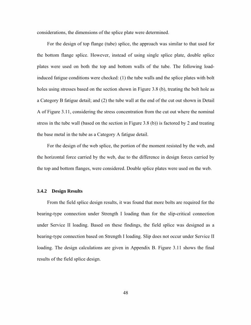
48
considerations, the dimensions of the splice plate were determined.
For the design of top flange (tube) splice, the approach was similar to that used for
the bottom flange splice. However, instead of using single splice plate, double splice
plates were used on both the top and bottom walls of the tube. The following load-
induced fatigue conditions were checked: (1) the tube walls and the splice plates with bolt
holes using stresses based on the section shown in Figure 3.8 (b), treating the bolt hole as
a Category B fatigue detail; and (2) the tube wall at the end of the cut out shown in Detail
A of Figure 3.11, considering the stress concentration from the cut out where the nominal
stress in the tube wall (based on the section in Figure 3.8 (b)) is factored by 2 and treating
the base metal in the tube as a Category A fatigue detail.
For the design of the web splice, the portion of the moment resisted by the web, and
the horizontal force carried by the web, due to the difference in design forces carried by
the top and bottom flanges, were considered. Double splice plates were used on the web.
3.4.2 Design Results
From the field splice design results, it was found that more bolts are required for the
bearing-type connection under Strength I loading than for the slip-critical connection
under Service II loading. Based on these findings, the field splice was designed as a
bearing-type connection based on Strength I loading. Slip does not occur under Service II
loading. The design calculations are given in Appendix B. Figure 3.11 shows the final
results of the field splice design.
49
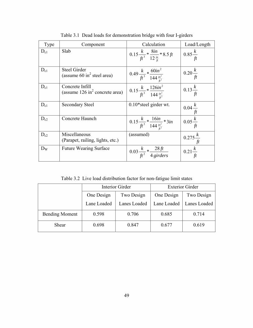
Table 3.1 Dead loads for demonstration bridge with four I-girders
Type Component Calculation Load/Length Dc1 Slab
ft.*in*ftk.
ftin
58128150 3
ftk85.0
Dc1 Steel Girder (assume 60 in2 steel area)
2
214460*49.0
2
3ftin
inftk ft
k20.0
Dc1 Concrete Infill (assume 126 in2 concrete area)
2
2144126150
2
3ftin
in*ftk. ft
k.130
Dc1 Secondary Steel 0.10*steel girder wt. ftk.040
Dc2 Concrete Haunch inin
ftk
ftin
3*14416*15.0
2
23 ftk05.0
Dc2 Miscellaneous (Parapet, railing, lights, etc.)
(assumed) ftk275.0
DW Future Wearing Surface girders
ftftk
428*03.0 2
ftk21.0
Table 3.2 Live load distribution factor for non-fatigue limit states
Interior Girder Exterior Girder
One Design
Lane Loaded
Two Design
Lanes Loaded
One Design
Lane Loaded
Two Design
Lanes Loaded
Bending Moment 0.598 0.706 0.685 0.714
Shear 0.698 0.847 0.677 0.619

50
Table 3.3 Live load distribution factor for Fatigue limit state
Interior Girder Exterior Girder
One Design
Lane Loaded
Two Design
Lanes Loaded
One Design
Lane Loaded
Two Design
Lanes Loaded
Bending Moment 0.498 - 0.571 -
Shear 0.582 - 0.564 -
Table 3.4 Load factors and load combinations
Limit state DC DW LL+IM
Strength I 1.25 1.50 1.75
Constructability 1.50 - -
Service II 1.00 1.00 1.30
Fatigue - - 0.75
Table 3.5 Performance ratios for positive moment section
Limit State Performance Ratio (Load Effect/Resistance) Controlling Design Check
Strength I 0.82 Flexure
Constructability 0.79 Lateral-Torsional Buckling
Service II 0.88 Flexure (Bottom Flange)
Fatigue 0.73 Transverse Stiffeners

51
Figure 3.1 Demonstration bridge cross-section
52
Step 1: Place four girders with temporary bracing on one span
Step 2: Place four girders with temporary bracing on the other span
Step 3: Place permanent diaphragms
Step 4: Place pre-cast concrete deck except at splice location
Step 5: Make field splice
Step 6: Place pre-cast concrete deck at splice location and complete deck
Figure 3.2 Option 1 for construction sequence of bridge (Construction Option 1)
53
Step 1: Place four girders with temporary bracing on one span
Step 2: Place four girders with temporary bracing on the other span
Step 3: Place permanent diaphragms
Step 4: Make field splice
Step 5: Place and complete pre-cast concrete deck (or cast-in-place deck)
Figure 3.3 Option 2 for construction sequence of bridge (Construction Option 2)

54
-3000
-2000
-1000
0
1000
2000
3000
0 20 40 60 80 100Distance from end bearing(ft)
Mom
ent(
k-ft
)
DC1DC2DW +(LL+IM) -(LL+IM)
Figure 3.4 Unfactored dead and live load moment envelopes for Construction Option 1
-150
-100
-50
0
50
100
150
0 20 40 60 80 100Distance from end bearing(ft)
Shea
r(k)
DC1DC2DW +(LL+IM) -(LL+IM)
Figure 3.5 Unfactored dead and live load shear envelopes for Construction Option 1
55
-3000
-2000
-1000
0
1000
2000
3000
0 20 40 60 80 100Distance from end bearing(ft)
Mom
ent(
k-ft
)
DC1DC2DW +(LL+IM) -(LL+IM)
Figure 3.6 Unfactored dead and live load moment envelopes for Construction Option 2
-150
-100
-50
0
50
100
150
0 20 40 60 80 100Distance from end bearing(ft)
Shea
r(k)
DC1DC2DW +(LL+IM) -(LL+IM)
Figure 3.7 Unfactored dead and live load shear envelopes for Construction Option 2

56
Short-termPost-tensionedstrand
Short-term
(b) Section used for transformed section analysis of negative bending stresses at pier splice
(a) Section used for section ultimate flexural strength analysis of negative bending at pier splice
(c) Section used for transformed section analysis of negative bending stresses adjacent to pier splice
Figure 3.8 Sections considered for pier section design
-4000
-3000
-2000
-1000
0
1000
2000
0 20 40 60 80 100Distance from end bearing(ft)
Mom
ent(
k-ft
)
: bracing points
Figure 3.9 Factored moment envelopes due to Strength I loading
for Construction Option 1
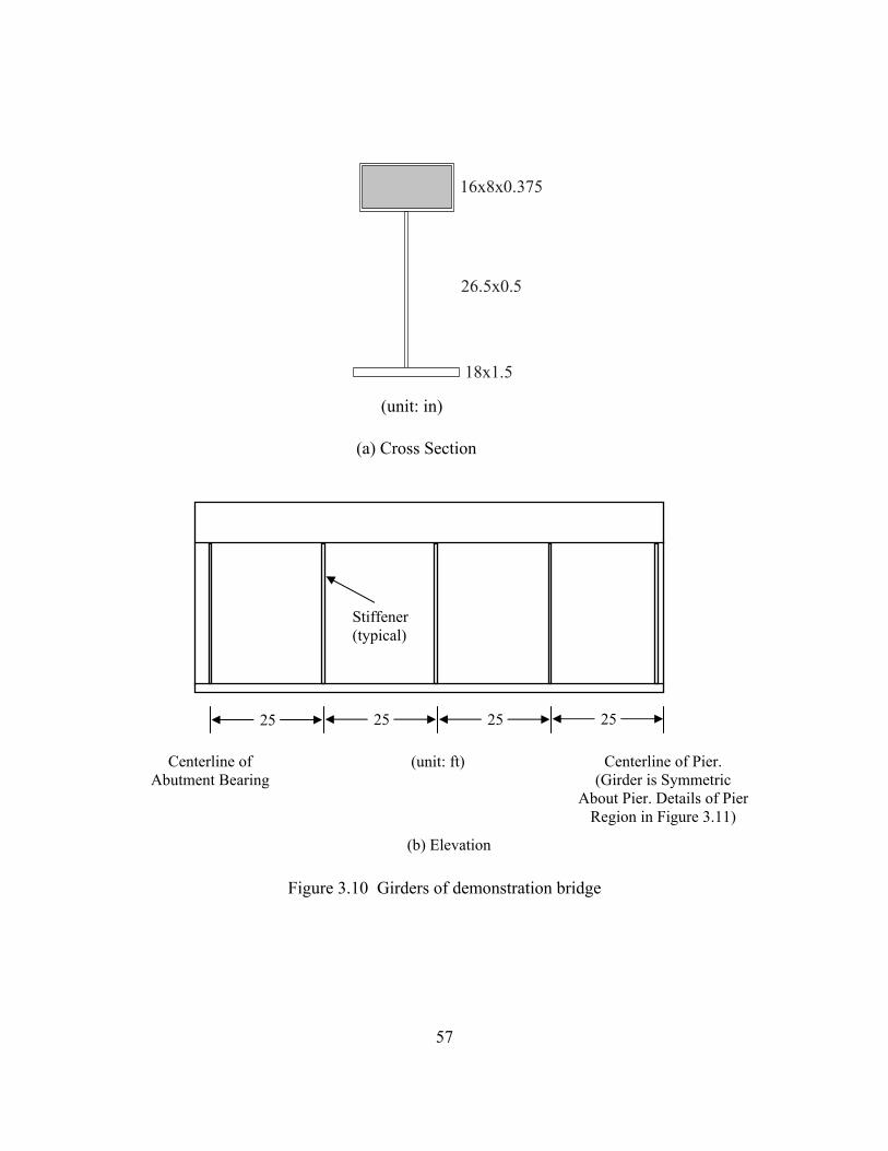
57
Figure 3.10 Girders of demonstration bridge
25 25 25 25
Centerline of Abutment Bearing
Centerline of Pier. (Girder is Symmetric
About Pier. Details of Pier Region in Figure 3.11)
Stiffener (typical)
(b) Elevation
(unit: ft)
(unit: in)
16x8x0.375
26.5x0.5
18x1.5
(a) Cross Section
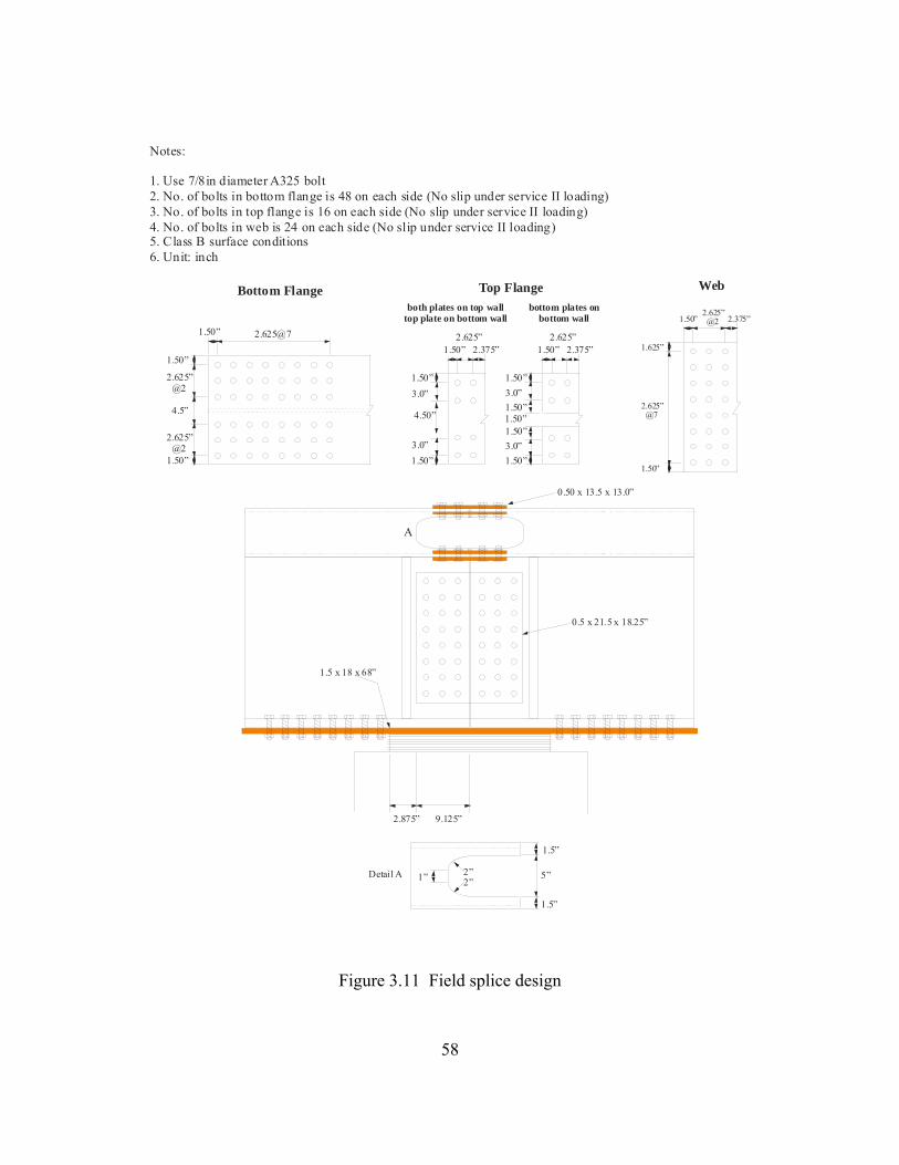
58
Figure 3.11 Field splice design
1.625”
1.50”
2.625” @7
1.50”2.625” @2 2.375”
Notes:
1. Use 7/8in diameter A325 bolt2. No. of bolts in bottom flange is 48 on each side (3. No. of bolts in top flange is 16 on each side
No slip under service II loading)(No slip under service II loading)
4. No. of bolts in web is 24 on each side (No slip under service II loading)5. Class B surface conditions6. Unit: inch
9.125”
1.5 x 18 x 68”
0.5 x 21.5 x 18.25”
1.50”
1.50”
2.625” @2
2.625” @2
4.5”
1.50” 2.625@7
Bottom Flange Web
2.875”
1.50”2.625” 2.375”
1.50”
1.50”
4.50”
1.50”2.625” 2.375”
1.50”
1.50”
1.50”1.50”
1.50”
3.0”3.0”
3.0”3.0”
both plates on top walltop plate on bottom wall
bottom plates onbottom wall
0.50 x 13.5 x 13.0”
Top Flange
A
Detail A
1.5”
1.5”
5”1” 2”2”
59
CHAPTER 4 PRELIMINARY DESIGN OF PRECAST CONCRETE DECK
4.1 INTRODUCTION
To promote accelerated construction, the demonstration bridge was designed to be
built with precast deck panels. This design reduces the effort needed to cast a concrete
deck in the field, including installation of forms and steel reinforcement. This deck
design also eliminates the time (weeks) required for the concrete to cure. The preliminary
design of the precast concrete deck uses concepts and procedures outlined by Shelala
(2006) and some details in a test specimen deck described by Kim and Sause (2005).
4.2 DESIGN PROCEDURES
The precast concrete deck consists of twenty five precast panels, which are the full
width of the bridge deck. The size of the panels was selected based on shipping and
handling considerations. Each precast concrete panel is 8 in thick, 31.375 ft wide, and 8 ft
long. A general view of the precast concrete deck system is shown in Figure 4.1. The
panels were designed with a compressive strength of 4 ksi, but higher strength could be
easily achieved in a precast concrete plant. Each panel is designed with mild steel
reinforcing bars, pre-tensioned strands, and post-tensioned strands.
The mild steel reinforcing bars were designed as if the concrete deck system was a
cast-in-place (CIP) deck, and the equivalent strip method was used (Shelala 2006). For
the equivalent strip method analysis, the girders act as supports, and the deck acts as a
continuous beam spanning from support to support. In the transverse direction, which is
perpendicular to the girders, the interior spans and the overhangs were designed for live

60
load moments determined using Table A4-1 in Appendix A4 of Chapter 4 of the
AASHTO LRFD Bridge Design Specifications (AASHTO 2004). The table provides
positive and negative live load moments, based on girder spacing and distance from the
center of the girder to the design section for negative moment. The flexural strength of
the deck was checked for the Strength I limit state load combination, and flexural
cracking was checked with allowable stress in the tensile reinforcement for the Service II
limit state load combination.
In the longitudinal direction of the girders, the mild steel reinforcing bars located in
the lower layer were designed to satisfy the distribution requirement. This reinforcement
is considered secondary reinforcement, and has an effect on distributing the wheel loads
in the longitudinal direction of the girders to the primary reinforcement in the transverse
direction. The mild steel reinforcing bars located in the upper layer were designed to
satisfy temperature and shrinkage requirements.
Pre-tensioned strands were included in the transverse direction of the deck. These
strands were designed to prevent cracking of the deck panels in the transverse direction
(i.e., longitudinally oriented cracks) caused by the shipping and handling of the panels.
To create continuity between the panels (i.e., to prevent the transverse joints from
opening and closing), the deck is post-tensioned in the longitudinal direction after all
panels are in place on the girders. The post-tensioned strands were designed to keep the
critical transverse joint, that is, the joint between the middle panel over the pier and the
adjacent panel, closed. This critical joint is under maximum tension from the negative
bending moment, and no mild steel reinforcing bars cross this joint (or the other joints).
Opening of this joint was checked for the Service II limit state loading. This check
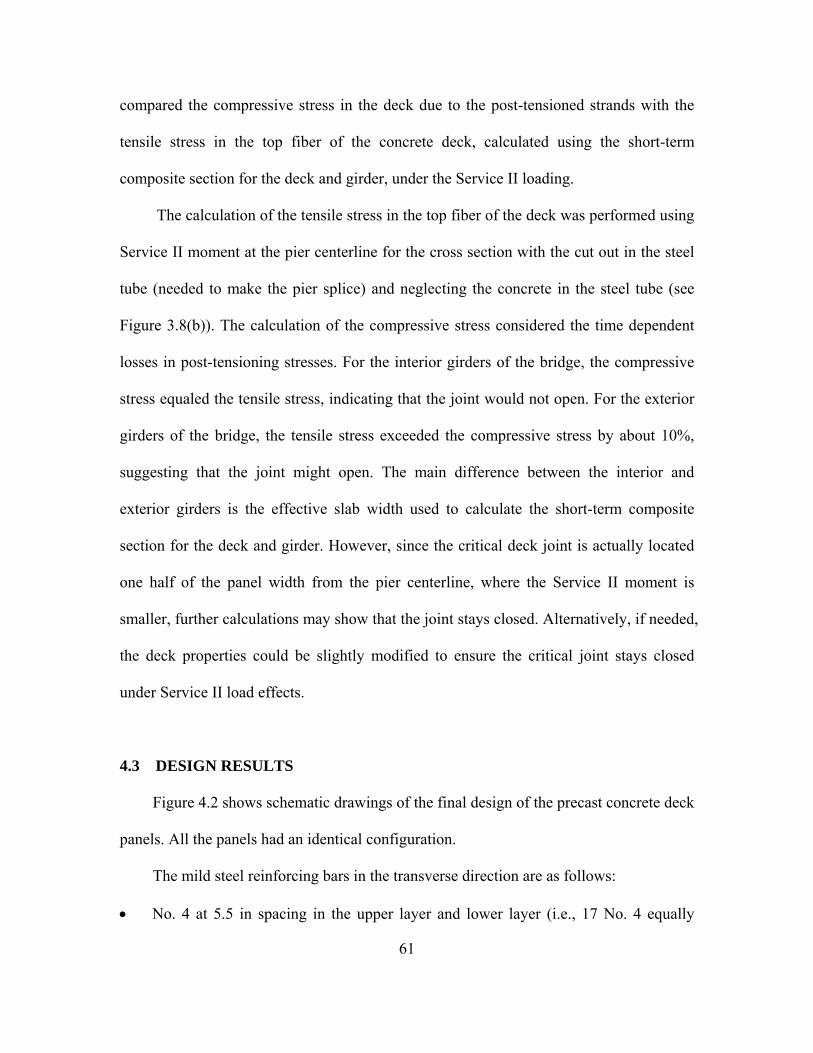
61
compared the compressive stress in the deck due to the post-tensioned strands with the
tensile stress in the top fiber of the concrete deck, calculated using the short-term
composite section for the deck and girder, under the Service II loading.
The calculation of the tensile stress in the top fiber of the deck was performed using
Service II moment at the pier centerline for the cross section with the cut out in the steel
tube (needed to make the pier splice) and neglecting the concrete in the steel tube (see
Figure 3.8(b)). The calculation of the compressive stress considered the time dependent
losses in post-tensioning stresses. For the interior girders of the bridge, the compressive
stress equaled the tensile stress, indicating that the joint would not open. For the exterior
girders of the bridge, the tensile stress exceeded the compressive stress by about 10%,
suggesting that the joint might open. The main difference between the interior and
exterior girders is the effective slab width used to calculate the short-term composite
section for the deck and girder. However, since the critical deck joint is actually located
one half of the panel width from the pier centerline, where the Service II moment is
smaller, further calculations may show that the joint stays closed. Alternatively, if needed,
the deck properties could be slightly modified to ensure the critical joint stays closed
under Service II load effects.
4.3 DESIGN RESULTS
Figure 4.2 shows schematic drawings of the final design of the precast concrete deck
panels. All the panels had an identical configuration.
The mild steel reinforcing bars in the transverse direction are as follows:
• No. 4 at 5.5 in spacing in the upper layer and lower layer (i.e., 17 No. 4 equally
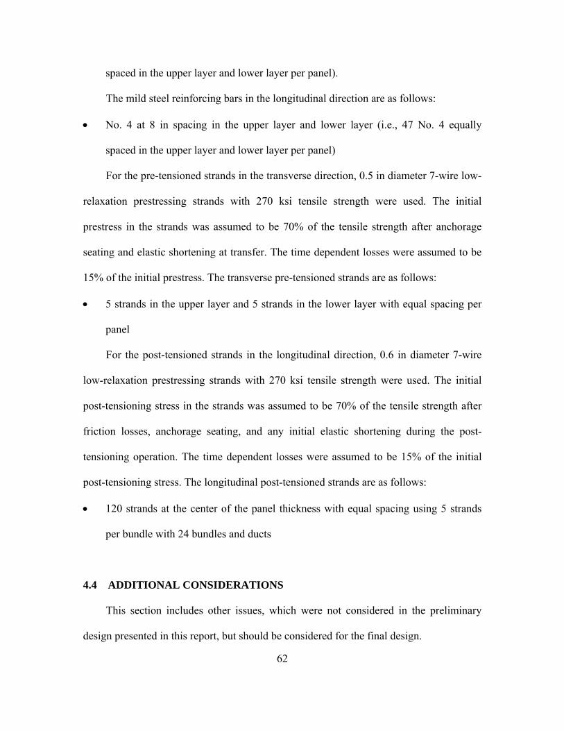
62
spaced in the upper layer and lower layer per panel).
The mild steel reinforcing bars in the longitudinal direction are as follows:
• No. 4 at 8 in spacing in the upper layer and lower layer (i.e., 47 No. 4 equally
spaced in the upper layer and lower layer per panel)
For the pre-tensioned strands in the transverse direction, 0.5 in diameter 7-wire low-
relaxation prestressing strands with 270 ksi tensile strength were used. The initial
prestress in the strands was assumed to be 70% of the tensile strength after anchorage
seating and elastic shortening at transfer. The time dependent losses were assumed to be
15% of the initial prestress. The transverse pre-tensioned strands are as follows:
• 5 strands in the upper layer and 5 strands in the lower layer with equal spacing per
panel
For the post-tensioned strands in the longitudinal direction, 0.6 in diameter 7-wire
low-relaxation prestressing strands with 270 ksi tensile strength were used. The initial
post-tensioning stress in the strands was assumed to be 70% of the tensile strength after
friction losses, anchorage seating, and any initial elastic shortening during the post-
tensioning operation. The time dependent losses were assumed to be 15% of the initial
post-tensioning stress. The longitudinal post-tensioned strands are as follows:
• 120 strands at the center of the panel thickness with equal spacing using 5 strands
per bundle with 24 bundles and ducts
4.4 ADDITIONAL CONSIDERATIONS
This section includes other issues, which were not considered in the preliminary
design presented in this report, but should be considered for the final design.

63
The panels should be cast with voids or pockets at girder location. These pockets
house the shear studs, providing the composite connection to the supporting girders. The
pocket dimensions are dependent on the width of the top flange and the number of rows
of shear studs placed in each pocket. Figure 4.3 shows the schematic drawings of the
precast concrete deck panels with pockets. As shown in this figure, each panel is assumed
to have 8 pockets (2 pockets per girder), and some of the mild steel reinforcing bars in the
transverse direction and the longitudinal direction can be excluded because of the
contribution of the pre-tensioned strands and post-tensioned strands, respectively. The
mild steel reinforcing bars and pre-tensioned strands are relocated to provide the pocket
space.
The panels should be leveled to eliminate eccentricity when the panels are post-
tensioned longitudinally. One possible option is to use leveling bolts cast into the panels.
A minimum of two leveling bolts per girder is suggested to be used to allow the dead
load of the precast panels to be distributed to each support girder. Grout may be needed
for the joints between panels, and the joints should be detailed for this grout.
In the preliminary precast deck design, the longitudinal post-tensioned strands run
the full length of the deck to permit post-tensioning from the ends. Therefore, the
concrete deck has a significant longitudinal prestress (approximately 1.4 ksi) in the
positive moment region (before dead loads Dc2b and Dw and live loads are on the bridge).
This concrete prestress was not considered in the positive moment region girder design.
Further design calculations should be made to consider the effect of the deck prestress on
the flexural strength of the positive moment cross section and to consider the effect of
creep due to prestress on the positive moment region section behavior. If the longitudinal

64
prestress needs to be reduced, some of the post-tensioned strands can be debonded in the
positive moment region.

65
Longitudinal direction
Transverse direction
Girder
Field spliceat pier section
Prec
ast c
oncr
ete
deck
pan
els
(8 ft
@ 2
5 =
200
ft)
Figure 4.1 General overview of precast concrete deck system
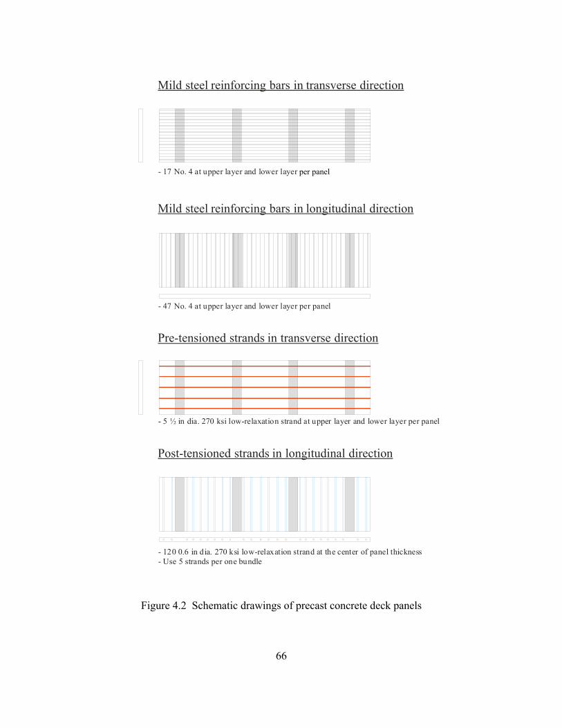
66
Figure 4.2 Schematic drawings of precast concrete deck panels
Mild steel reinforcing bars in transverse direction
Mild steel reinforcing bars in longitudinal direction
Pre-tensioned strands in transverse direction
Post-tensioned strands in longitudinal direction
- 17 No. 4 at upper layer and lower layer
- 47 No. 4 at per panelupper layer and lower layer
- 5 ½ in dia. 270 ksi low-relaxation strand at per panelupper layer and lower layer
- 120 0.6 in dia. 270 ksi low-relaxation strand at the center of panel thickness- Use 5 strands per one bundle
per panel

67
Figure 4.3 Schematic drawings of precast concrete deck panels including pockets
Pre-tensioned strands in transverse direction
Post-tensioned strands in longitudinal direction
Mild steel reinforcing bars in transverse direction
- 12 No. 4 at upper layer and lower layer
Mild steel reinforcing bars in longitudinal direction
- 35 No. 4 at per panelupper layer and lower layer
- 5 ½ in dia. 270 ksi low-relaxation strand at per panelupper layer and lower layer
- 120 0.6 in dia. 270 ksi low-relaxation strand at the center of panel thickness- Use 5 strands per one bundle
per panel

68
CHAPTER 5 FINITE ELEMENT SIMULATION OF CFTFGS DURING
DEMONSTRATION BRIDGE CONSTRUCTION
5.1 INTRODUCTION
An analytical study of finite element (FE) models of the concrete-filled tubular
flange girders (CFTFGs) of the demonstration bridge was conducted. The study
simulated construction loading conditions before the field splice is made and before the
girders are connected with shear connectors to a concrete deck. Therefore, the FE models
were simple span girders. The results of the study validate the design criteria for the
lateral-torsion buckling strength of the arrangement of girders and diaphragms in the
demonstration bridge.
5.2 FE ANALYSIS MODELS
The FE models were developed using ABAQUS (ABAQUS 2002). To understand
the possible buckling modes, elastic buckling analyses of the FE models were conducted.
To investigate the flexural strength, nonlinear load-displacement analyses of the FE
models, including both material and geometric nonlinearity, were conducted.
As mentioned previously, simple span girders were analyzed. However, to
investigate the influence of adjacent girders, single girder and multiple girder models (i.e.,
two girders, three girders, and four girders) were developed and analyzed. Two different
diaphragm arrangements were also studied. Scheme 9 (S9) has three diaphragms,
including two end diaphragms and one interior diaphragm. Scheme 10 (S10) has only the
two end diaphragms. The diaphragms are W21X57 steel sections. The girder cross-

69
section used in the model is shown in Figure 3.10.
A simply supported boundary condition was applied both in plane and out of plane
at the locations of the bearing stiffeners at each end of each girder. This boundary
condition simulates the combined effect of the end diaphragms, bearing stiffeners, and
bearings to provide stiff lateral and torsional bracing at the bearings. A uniformly
distributed load was applied on top of the tube along the entire length to simulate the
weight of the girders, the weight of the diaphragms, and the weight of the deck.
The tube, web, and bottom flange were modeled using four node three-dimensional
shell (S4R) elements. The steel material was modeled using a linear elastic isotropic
model in the elastic range and the ABAQUS metal plasticity model in the inelastic range.
The plasticity model uses the Von Mises yield criterion, associated plastic flow theory,
and isotropic hardening. A simplified bilinear stress-strain curve with no strain hardening
was used. Residual stresses in the steel were not included.
The concrete infill was modeled using eight node three-dimensional solid (C3D8R)
elements. The concrete material was modeled using a linear elastic isotropic model in the
elastic range and a multiaxial plasticity model in the inelastic range. For the multiaxial
plasticity model, a linear Drucker-Prager model with a non-associated flow rule, and
isotopic hardening and softening behavior was used. The linear Drucker-Prager model is
defined by a stress-strain curve under uniaxial compression, and three parameters,
namely, the ratio of the yield stress in triaxial tension to the yield stress in triaxial
compression (K), the friction angle (β), and the dilation angle (ψ). An empirical stress-
strain model for unconfined concrete developed by Oh (2002) was used as the stress-
strain curve under uniaxial compression for the concrete infill. The value of K was

70
assumed to be 1. Values of β and ψ were determined by calibrating the compressive
strength of confined concrete to the empirical expression from Richart et al. (1928) and
calibrating the ratio of transverse strain to axial strain at the peak stress to the value of 0.4
proposed by Oh (2002). The resulting values of β and ψ were 56.7 and 15.0 degrees,
respectively.
The interface between the steel tube and concrete infill was modeled as a rigid
connection based on the results of the previous study by Kim and Sause (2005).
Initial geometric imperfections were introduced into the model for nonlinear load-
displacement analyses. The imperfection shapes were defined by scaling the buckling
mode shapes obtained from an elastic buckling analysis (see Table 5.1). Several
imperfection shapes were considered, and the shapes were scaled so the flange out-of-
straightness (sweep) had a magnitude of either L/1000 or L/2000. If the buckling mode is
a single half sine wave, only the magnitude of L/1000 was considered. However, if the
buckling mode is a double half sine wave, two cases, with magnitudes of L/1000 and
L/2000, respectively, were considered.
5.3 FE ANALYSIS RESULTS
Table 5.1 shows the elastic buckling analysis results for different FE models with
different numbers of girders and the two bracing arrangements, S9, with the interior
diaphragm, and S10, without the interior diaphragm. The buckling mode shape and the
elastic buckling strength (given as the maximum moment reached at mid-span) are
included in this table.
From the elastic buckling analysis results, the following observations were made:

71
• The buckling mode shape with a single half sine wave shape results in a smaller
buckling strength than the buckling mode shape with a double or triple half sine
wave shape.
• As the number of girders increases, the buckling strength increases due to
contributions of the diaphragms.
• The girders with the S9 bracing arrangement have larger buckling strengths than the
girders with the S10 bracing arrangement.
• For the multi girder systems, regardless of whether the girders buckle in a single or
double half sine wave, a symmetric buckling mode shape along the longitudinal axis
of the girder, in which the diaphragm is deformed in single curvature, results in a
smaller buckling strength than asymmetric buckling mode shape along the
longitudinal axis of the girder, in which the diaphragm is deformed in double
curvature.
• The smallest buckling strength, which is 49720 k-in is larger than the yield moment
of the girder (35401 k-in), so the elastic buckling results shown in the table do not
control the strength, which is controlled by inelastic buckling. The inelastic buckling
capacity is obtained from nonlinear load-displacement analysis.
Tables 5.2 through 5.5 show the nonlinear load-displacement analysis results. For
these analyses, different numbers of girders, different bracing arrangements, and different
imperfection modes and magnitudes were considered. The maximum moment (Mmax)
obtained from the analyses were compared with the yield moment (My = 35401 k-in) and
the plastic moment (Mp= 44709 k-in) obtained from a cross-section analysis; the mid-
span moment produced by the factored design loads for the construction loading

72
condition (1.5MDC = 26982 k-in, where MDC is the mid-span moment due to Dc1 and
Dc2a); and the design flexural strength (Mdbr which varies as the number of girders is
varied) obtained from the design flexural strength formula (Equation 2.8). Note that Mp is
calculated from simple plastic theory using an equivalent rectangular stress block for the
concrete in the steel tube and the yield stress for the steel.
Figures 5.1 compares the design flexural strength for single and multiple girders (i.e.,
two, three, and four girders) and the mid-span moment produced by the factored design
loads under the construction loading condition.
From the nonlinear load-displacement analysis results, the following observations
were made:
• The maximum moments obtained from the FE analyses are at least 42% larger than
the mid-span moment produced by the factored design loads.
• The maximum moments obtained from the FE analyses are at least 14% larger than
the design flexural strength for construction loading conditions.
Note that the design flexural strength equation for construction loading (Equation
2.8) was not developed to represent the maximum moment during lateral-torsional
buckling, but represents the minimum of: (1) the bending moment at the onset of lateral-
torsional instability, (which is the moment when an incremental strain reversal occurs at
any location on the cross-section due to lateral bending), and (2) the bending moment at
first yielding on the cross-section (Kim and Sause 2005). The moment at the onset of
instability or first yielding is always less than the maximum moment. This difference
produces the 14% difference between the maximum moment from the finite element
analyses and the design flexural strength from Equation (2.8)

73
From the above observation, it is concluded that the girders with either S10 or S9
bracing arrangement are safe under the construction loading conditions considered in the
study, and the actual strength under construction conditions is conservatively estimated
by the proposed design flexural strength equation.

74
Table 5.1 Elastic buckling analysis results
No of Girders
Bracing Type Buckling Mode & Buckling Strength (k-in)
- 1 -
49720 98180 173600 -
2 S10
51890 53790 98680 99120
- 2 S9
74450 99640 101000 -
3 S10
52720 56250 72780 98870
3 S9
93510 100180 102450 103267

75
Table 5.1 Elastic buckling analysis results (continued)
No of Girders
Bracing Type Buckling Mode & Buckling Strength (k-in)
52460 52650 54880 56190
4 S10
98810 98860 99400 99730
100100 100200 101900 103000
- - -
4 S9
105800 - - -
Table 5.2 Nonlinear load-displacement analysis results for single girder
No. of Bracing
Girders Arrangement Mode Mag.
1 L/1000 1.107 0.876 1.452 1.317
L/1000 1.102 0.873 1.446 1.311
L/2000 1.169 0.926 1.534 1.391
Mmax/Mdbr
1 S102
ImperfectionMmax/My Mmax/Mp Mmax/1.5MDC

76
Table 5.3 Nonlinear load-displacement analysis results for two girders
No. of Bracing
Girders Arrangement Mode Mag.
1 L/1000 1.084 0.859 1.423 1.290
2 L/1000 1.090 0.863 1.429 1.296
L/1000 1.105 0.875 1.450 1.315
L/2000 1.159 0.918 1.521 1.379
L/1000 1.105 0.875 1.450 1.315
L/2000 1.158 0.917 1.520 1.378
1 L/1000 1.174 0.930 1.540 1.282
L/1000 1.109 0.878 1.454 1.211
L/2000 1.174 0.929 1.540 1.282
L/1000 1.117 0.884 1.465 1.219
L/2000 1.177 0.932 1.544 1.286
Mmax/Mdbr
2
S10 3
4
S92
3
ImperfectionMmax/My Mmax/Mp Mmax/1.5MDC
Table 5.4 Nonlinear load-displacement analysis results for three girders
No. of Bracing
Girders Arrangement Mode Mag.
1 L/1000 1.080 0.855 1.417 1.285
2 L/1000 1.124 0.890 1.475 1.337
3 L/1000 1.170 0.927 1.536 1.392
L/1000 1.104 0.874 1.449 1.314
L/2000 1.159 0.918 1.521 1.379
L/1000 1.106 0.876 1.451 1.316
L/2000 1.169 0.925 1.533 1.390
L/1000 1.106 0.876 1.451 1.315
L/2000 1.168 0.925 1.532 1.389
1 L/1000 1.209 0.958 1.587 1.230
L/1000 1.128 0.893 1.480 1.148
L/2000 1.183 0.937 1.553 1.204
L/1000 1.126 0.891 1.477 1.145
L/2000 1.183 0.937 1.553 1.204
L/1000 1.142 0.904 1.499 1.162
L/2000 1.195 0.946 1.568 1.216
Mmax/Mdbr
3
S104
5
6
S9
2
3
4
ImperfectionMmax/My Mmax/Mp Mmax/1.5MDC

77
Table 5.5 Nonlinear load-displacement analysis results for four girders
No. of Bracing
Girders Arrangement Mode Mag.
1 L/1000 1.093 0.866 1.434 1.300
2 L/1000 1.086 0.860 1.425 1.292
3 L/1000 1.101 0.872 1.444 1.309
4 L/1000 1.112 0.881 1.459 1.323
L/1000 1.104 0.874 1.449 1.314
L/1000 1.145 0.906 1.502 1.362
L/1000 1.104 0.874 1.449 1.313
L/2000 1.165 0.922 1.528 1.386
L/1000 1.105 0.875 1.450 1.314
L/2000 1.165 0.923 1.529 1.386
L/1000 1.106 0.876 1.451 1.316
L/2000 1.168 0.925 1.532 1.389
L/1000 1.140 0.903 1.495 1.140
L/2000 1.192 0.944 1.564 1.192
L/1000 1.146 0.907 1.503 1.146
L/2000 1.198 0.949 1.572 1.198
L/1000 1.142 0.905 1.499 1.142
L/2000 1.198 0.949 1.572 1.198
L/1000 1.163 0.921 1.526 1.163
L/2000 1.210 0.958 1.588 1.210
5 L/1000 1.223 0.968 1.604 1.223
3
4
Mmax/Mdbr
4
S10
5
6
7
8
S9
1
2
ImperfectionMmax/My Mmax/Mp Mmax/1.5MDC

78
Figure 5.1 Design flexural strength for construction loading conditions
0
10000
20000
30000
40000
50000
0 500 1000 1500 2000 2500 3000 3500 4000
Span Length (in)
Flex
ural
Str
engt
h (k
-in)
S10S9(two girders)S9(three girders)S9(four girders)
Simple span length of demonstration bridge
Factoreddesign load
Design flexural strength (S9)
Design flexural strength (S10)
Factored design moment
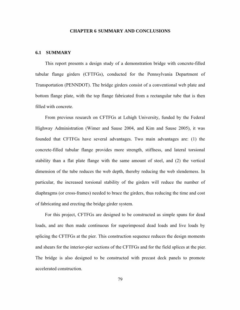
79
CHAPTER 6 SUMMARY AND CONCLUSIONS
6.1 SUMMARY
This report presents a design study of a demonstration bridge with concrete-filled
tubular flange girders (CFTFGs), conducted for the Pennsylvania Department of
Transportation (PENNDOT). The bridge girders consist of a conventional web plate and
bottom flange plate, with the top flange fabricated from a rectangular tube that is then
filled with concrete.
From previous research on CFTFGs at Lehigh University, funded by the Federal
Highway Administration (Wimer and Sause 2004, and Kim and Sause 2005), it was
founded that CFTFGs have several advantages. Two main advantages are: (1) the
concrete-filled tubular flange provides more strength, stiffness, and lateral torsional
stability than a flat plate flange with the same amount of steel, and (2) the vertical
dimension of the tube reduces the web depth, thereby reducing the web slenderness. In
particular, the increased torsional stability of the girders will reduce the number of
diaphragms (or cross-frames) needed to brace the girders, thus reducing the time and cost
of fabricating and erecting the bridge girder system.
For this project, CFTFGs are designed to be constructed as simple spans for dead
loads, and are then made continuous for superimposed dead loads and live loads by
splicing the CFTFGs at the pier. This construction sequence reduces the design moments
and shears for the interior-pier sections of the CFTFGs and for the field splices at the pier.
The bridge is also designed to be constructed with precast deck panels to promote
accelerated construction.

80
To accomplish the project, the following tasks were conducted: (1) develop design
criteria, (2) preliminary design of CFTFGs for the demonstration bridge, (3) preliminary
design of the field splice, (4) preliminary design of the precast concrete deck, and (5)
finite element analyses.
(1) Develop Design Criteria
Design criteria for CFTFGs were developed based on the results of previous
analytical and experimental investigations (Wimer and Sause 2004, Kim and Sause,
2005). The design criteria are generally compatible with the 2000 PENNDOT Design
Manual Part 4 (PENNDOT 2000) and the 2004 AASHTO LRFD Bridge Design
Specifications (AASHTO 2004).
(2) Preliminary Design of CFTFGs for Demonstration Bridge
A preliminary design of a two-span continuous composite tubular flange girder
bridge with spans of 100 ft-100 ft was developed. This study developed a preliminary
design of the critical positive moment section, the interior-pier section, and the field
splice. The CFTFGs were designed as simple spans for dead loads and continuous spans
for superimposed dead loads and live loads.
The demonstration bridge cross-section was provided by PENNDOT and consists of
four girders spaced at 8 ft-5.5 in centers with 3 ft overhangs. The concrete deck was 8 in.
thick. Grade 50 steel and concrete with a compressive strength of 4 ksi were used. The
design study considers the 2004 AASHTO LRFD Bridge Design Specifications
(AASHTO 2004) and the PENNDOT Design Manual Part 4 (PENNDOT 2000) as well
as the design criteria developed by the project. The design study results are based on
several assumptions: (1) end diaphragms, but no interior diaphragms within the spans

81
under construction conditions (during erection and deck placement) and one interior
diaphragm at mid-span under service conditions, (2) bearing stiffeners and three equally-
spaced intermediate transverse stiffeners (per span) with Category C′ fatigue details, (3)
similar cross-sections for the positive moment section and the pier section, and (4) a field
splice located at the pier section.
(3) Preliminary Design of Field Splice
The demonstration bridge is a two-span bridge with a field splice located at the pier.
A preliminary design of the bolted field splice located at the pier was provided.
(4) Preliminary Design of Precast Concrete Deck
To promote accelerated construction, the demonstration bridge deck was designed to
be built with precast concrete deck panels. The size of the panels was selected based on
shipping and handling considerations. The panels were designed with a concrete
compressive strength of 4 ksi, but higher strength could be easily achieved in a precast
concrete plant. Each panel was designed with mild steel reinforcing bars, pre-tensioned
strands, and post-tensioned strands.
(5) Finite Element Analyses
An analytical study of finite element (FE) models of the concrete-filled tubular
flange girders (CFTFGs) of the demonstration bridge was conducted under simulated
construction loading conditions using ABAQUS (ABAQUS 2002). Conditions before the
field splice is made and before the girders are connected with shear connectors to the
precast concrete deck were simulated. Therefore, the FE models were simple span girders
non-composite with the deck.
To understand the possible buckling modes, elastic buckling analyses of the FE

82
models were conducted. To investigate the lateral-torsional buckling strength, nonlinear
load-displacement analyses of the FE models, including both material and geometric
nonlinearity, were conducted. Single girder and multiple girder models (i.e., two girders,
three girders, and four girders) were developed and analyzed to investigate the influence
of adjacent girders. Two different diaphragm arrangements were studied. Scheme 9 (S9)
has three diaphragms, including two end diaphragms and one interior diaphragm. Scheme
10 (S10) has only the two end diaphragms.
The FE analyses validated the design criteria and validated the preliminary design of
the demonstration bridge for the construction conditions that were considered.
6.2 CONCLUSIONS
Based on the results of the accomplished tasks, the following conclusions are drawn:
• The CFTFGs designed for the demonstration bridge have enough lateral torsional
stability under the construction loading conditions that were considered, even with
no interior bracing within the span, so that fabrication and erection effort can be
reduced by eliminating diaphragms.
• The field splice at the pier can simplify fabrication and erection, and reduce the
dead load effects at the pier section. With this splice, the CFTFGs are constructed
as simple spans for the weight of the CFTFGs and the bridge deck, but are made
continuous for superimposed dead loads and live loads. As a result, the design
moments and shears for the interior-pier section and for the field splice at the pier
are reduced.
• The precast concrete deck can reduce the time needed for construction, compared to
83
a cast-in-place concrete deck, by reducing the time needed to place forms and
reinforcing steel, and eliminating the time needed for the concrete to cure.
• The CFTFGs designed for the demonstration bridge with either the S9 (one interior
diaphragm and two end diaphragms) or the S10 (no interior diaphragm and two end
diaphragms) bracing arrangement are adequate for the construction loading
conditions that were considered in the study.
84
REFERENCES
ABAQUS (2002). ABAQUS/Standard User’s Manuals: Volume I – III, Hibbitt, Karlsson,
and Sorenson, Inc., Pawtucket, Rhode Island.
AASHTO (1998). LRFD Bridge Design Specifications, American Association of State
Highway and Transportation Officials, Washington, D.C.
AASHTO (2004). LRFD Bridge Design Specifications, American Association of State
Highway and Transportation Officials, Washington, D.C.
Kim, B.-G. and Sause, R. (2005). “High Performance Steel Girders with Tubular
Flanges,” ATLSS Report, 05-15, ATLSS Research Center, Lehigh University,
Bethlehem, PA.
Oh, B. (2002). “A Plasticity Model for Confined Concrete under Uniaxial Loading,”
Ph.D. Dissertation, Department of Civil and Environmental Engineering, Lehigh
University, Bethlehem, PA.
PENNDOT (2000). Design Manual Part 4 (DM-4), Structures Procedures-Design-Plans
Presentation PDT-PUB No. 15M, Commonwealth of Pennsylvania, Department of
Transportation.
Richart, F.E., Brandtzaeg, A., and Brown, R.L. (1928). “A Study of the Failure of
Concrete under Combined Compressive Stresses,” Engineering Experiment Station,
Bulletin No. 185, University of Illinois-Urbana Champaign, IL.
Sause, R., and Fisher, J.W. (1996). “Application of High-Performance Steel in Bridges,”
Proceedings, 12th U.S.-Japan Bridge Engineering Workshop, Buffalo, New York,
October 1996, pp. 317-331.

85
Shelala, J. (2006). M.S. Thesis (in progress), Department of Civil and Environmental
Engineering, Lehigh University, Bethlehem, PA.
Wassef, W.G., Ritchie, P.A., and Kulicki, J.M. (1997). “Girders with Corrugated Webs
and Tubular Flanges – An Innovative Bridge System,” Proceedings, 14th Annual
Meeting, International Bridge Conference, Pittsburgh, Pennsylvania, June 1997, pp.
425-432.
Wimer, M. and Sause, R. (2004). “Rectangular Tubular Flange Girders with Corrugated
and Flat Webs,” ATLSS Report 04-18, ATLSS Research Center, Lehigh University,
Bethlehem, PA.
Yura, J.A., Philips, B., Raju, S., and Webb, S. (1992). “Bracing of Steel Beams in
Bridges,” Research Report 1239-4F, Center for Transportation Research, University
of Texas at Austin, Austin, TX..

Appendix A. Positive Moment Region Preliminary DesignBRIDGE PARAMETERS (yellow highlight indicates input data)Description: Two span continuous (for superimposed dead load and live load) composite CFTFG with each span of 100 ft andwidth of 31 ft - 4.5 in. The bridge cross section consists of 4 girders spaced at 8 ft - 5.5 in with 3 ft overhangs.
Bridge Width (in) Span Length (in) Girder Spacing (in) Number of girders Overhang (from girder centerline) (in)
W 376.5:= L 1200:= s 101.5:= ng 4:= se 36:=
Yield Strength (ksi) Young's Modulus (ksi) Concrete Strength (ksi) Slab Thickness (in) Haunch Thickness (in)
Fy 50:= Rh 1:= E 29000:= fcprime 4:= Tslab 8:= Thaunch 3:=
Concrete Modulus (ksi) Modular ratio (input) Modular ratio (actual) Long-term modular ratio Resistance Factor
Ec57000 fcprime 1000⋅⋅
1000:= n 8:= ns n:=
EEc
8.044= nl 3 n⋅:= Φ 1.0:=
MAXIMUM UNFACTORED MOMENTS DUE TO UNFACTORED LOADS DC1 is weight of girders, slab, and bracing. DC2 is weight of haunch and barrier. DW is weight of wearing surface. Note that DC1acts on simple spans and the max positive moment is at midspan. Remaining dead load and live load act on continuous spans andthe max positive moment is at 40 ft. from abutment bearings (analysis of sections spaced at 10 ft). For simplicity, these moments aretreated as if they act at the same section. More accurate calculations would consider each section separately.Mdc1_pos 18300:= kip*in Mdc2_pos 2730:= kip*in Mdw_pos 1764:= kip*in Mll_pos 19232:= kip*in
moment applied to non-compositesection including haunchMDC Mdc1_pos
0.0500.275 0.050+
⎛⎜⎝
⎞⎟⎠
Mdc2_pos⋅+⎡⎢⎣
⎤⎥⎦
:= MDC 18720= kip*in
MAXIMUM FATIGUE + IMPACT MOMENT Mfat_pos 8325:= kip*in
MAXIMUM UNFACTORED SHEAR FORCES DUE TO UNFACTORED LOADS Vdc1_pos 61:= kips Vdc2_pos 12.19:= kips Vdw_pos 7.88:= kips Vll_pos 93.44:= kips
shear applied to non-compositesection including haunchVDC Vdc1_pos
0.0500.275 0.050+
⎛⎜⎝
⎞⎟⎠
Vdc2_pos⋅+⎡⎢⎣
⎤⎥⎦
:= VDC 62.9= kips
MAXIMUM FATIGUE + IMPACT SHEAR FORCESVfat_pos 38.2:= kips Vfat_neg 42.6−:= kips
FACTORED LOAD COMBINATIONSMconst_pos 1.5 MDC⋅:= Mconst_pos 28080= kip*in
MstI_pos 1.25 Mdc1_pos⋅ 1.25 Mdc2_pos⋅+ 1.5 Mdw_pos⋅+ 1.75 Mll_pos⋅+( ) 0.95⋅:= MstI_pos 59460= kip*in
MsvII_pos 1.0 Mdc1_pos⋅ 1.0 Mdc2_pos⋅+ 1.0 Mdw_pos⋅+ 1.3 Mll_pos⋅+:= MsvII_pos 47795.6= kip*in
Mfat_pos 0.75 Mfat_pos⋅:= Mfat_pos 6243.8= kip*in
Vconst_pos 1.5VDC:= Vconst_pos 94.3= kips
VstI_pos 1.25 Vdc1_pos⋅ 1.25 Vdc2_pos⋅+ 1.5 Vdw_pos⋅+ 1.75 Vll_pos⋅+( ) 0.95⋅:= VstI_pos 253.5= kips
Vfat_pos Vdc1_pos Vdc2_pos+ Vdw_pos+ 2 0.75 Vfat_pos⋅( )+:= Vfat_pos 138.4= kips
GIRDER DIMENSIONSTube horizontal plate thickness Tube vertical plate thickness Bottom flange thickness Web thickness
Tt138
:= inches Tt238
:= inches Tbf 1.5:= inches Tweb816
:= inches
Tube horizontal plate width Tube vertical plate width Bottom flange width
Bt1 16:= inches Bt2 7.25:= inches Bbf 18:= inches
A-1

Web depth Dweb 36 2 Tt1⋅− Bt2− Tbf−:= Dweb 26.5= inches
Total girder depth Dgirder Tbf Dweb+ 2 Tt1⋅+ Bt2+:= Dgirder 36= inches
Depth including deck Dtotal Dgirder Thaunch+ Tslab+:= Dtotal 47= inches
GIRDER AREAS
Abf Bbf Tbf⋅:= Abf 27= in2 Area of bottom flange
Atube 2 Tt1⋅ Bt1⋅ 2 Tt2⋅ Bt2⋅+:= Atube 17.44= in2 Area of tube
Aw Dweb Tweb⋅:= Aw 13.25= in2 Area of web
Asteel Aw Atube+ Abf+:= Asteel 57.69= in2 Total steel area
AconBt2 Bt1 2 Tt2⋅−( )⋅
ns:= Acon 13.82= in2 Equivalent area of concrete in tube (short term)
AclongBt2 Bt1 2 Tt2⋅−( )⋅
nl:= Aclong 4.607= in2 Equivalent area of concrete in tube (long term)
EFFECTIVE WIDTH OF SLAB (INTERIOR GIRDER)
beff1L4
:= beff1 300= beff2 s:= beff2 101.5= beff3 12 Tslab⋅Bt12
+:= beff3 104=
The smallest beff governsBeffi beff1 beff1 beff2≤ beff1 beff3≤∧if
beff2 beff2 beff1≤ beff2 beff3≤∧if
beff3 otherwise
:=
Beffi 101.5= in
EFFECTIVE WIDTH OF SLAB (EXTERIOR GIRDER)
beff4s2
⎛⎜⎝
⎞⎟⎠
se+:= beff4 86.75=
The smallest beff governsBeffe beff1 beff1 beff2≤ beff1 beff3≤∧if
beff4 beff4 beff1≤ beff4 beff3≤∧if
beff3 otherwise
:=
Beffe 86.75= in
SELECT EFFECTIVE WIDTH OF SLAB (use Beffi for interior girder, Beffe for exterior girder, or minimum)
Beff min Beffe Beffi, ( ):= Beff 86.75= Note: here the minimum is used, which is for an exterior girder.
TUBE THICKNESS REQUIREMENT
Ct1Bt1 2 Tt2⋅−
Tt1:= Ct1 40.67= Ct2
Bt2Tt2
:= Ct2 19.33= Dt 1.7EFy
⋅:= Dt 40.94=
Ratiotubethickness1Ct1
Dt:= Ratiotubethickness1 0.993= Ratiotubethickness2
Ct2
Dt:= Ratiotubethickness2 0.472=
Ratiotubethickness Ratiotubethickness1 Ratiotubethickness1 Ratiotubethickness2>if
Ratiotubethickness2 otherwise
:=
Ratiotubethickness 0.993= < 1 therefore wall thickness is okay
MINIMUM DEPTH OF GIRDER
A-2

Dgirdermin 0.027 L⋅:= Dgirdermin 32.4= inches Dgirder 36= > Dgirdermin 32.4= o.k.
CONSTANT FOR CALCULATING KT
β .257:= β is a constant dependent upon (Bt1-2*Tt2)/Bt2
SECTION PROPERTIES
Calculate the elastic neutral axis for1. Noncomposite steel section with short term concrete (n) and with long term concrete (3n) in tube2. Short term composite (with deck) section (n) with short term concrete (n) in tube3. Long term composite (with deck) section (3*n) with long term concrete (3*n) in tube
1. Steel section elastic neutral axis (reference line taken at the top of the top flange)
Assuming short term concrete in tube
Agirder Acon Atube+ Aw+ Abf+:=
ENAgirder
Acon Tt1Bt22
+⎛⎜⎝
⎞⎟⎠
⋅ Atube Tt1Bt22
+⎛⎜⎝
⎞⎟⎠
⋅+ Aw 2 Tt1⋅ Bt2+Dweb
2+⎛⎜
⎝⎞⎟⎠
⋅+ Abf 2 Tt1⋅ Bt2+ Dweb+Tbf
2+⎛⎜
⎝⎞⎟⎠
⋅+
Agirder:=
ENAgirder 19.00= in from the top of the girder <== short term concrete in tube
Assuming long term concrete in tube
Agirderlong Aclong Atube+ Aw+ Abf+:=
ENAgirderlong
Aclong Tt1Bt22
+⎛⎜⎝
⎞⎟⎠
⋅ Atube Tt1Bt22
+⎛⎜⎝
⎞⎟⎠
⋅+ Aw 2 Tt1⋅ Bt2+Dweb
2+⎛⎜
⎝⎞⎟⎠
⋅+ Abf 2 Tt1⋅ Bt2+ Dweb+Tbf
2+⎛⎜
⎝⎞⎟⎠
⋅+
Agirderlong:=
ENAgirderlong 21.21= in from the top of the girder <== long term concrete in tube
Assuming no concrete in tube
Agirdernoconc Atube Aw+ Abf+:=
ENAgirdernoconc
Atube Tt1Bt22
+⎛⎜⎝
⎞⎟⎠
⋅ Aw 2 Tt1⋅ Bt2+Dweb
2+⎛⎜
⎝⎞⎟⎠
⋅+ Abf 2 Tt1⋅ Bt2+ Dweb+Tbf
2+⎛⎜
⎝⎞⎟⎠
⋅+
Agirdernoconc:=
ENAgirdernoconc 22.59= in from the top of the girder <== no concrete in tube
2. Short term elastic neutral axis (reference line taken at the top of the concrete deck)
ENA(short) = the elastic neutral axis of the short term composite (with deck) section with short term concrete in tube
Btr(hshort) = transformed width of the haunch for short term composite section
Btr(short) = transformed width of the slab for the short term composite section(here taken as zero to neglect haunch area, otherwise =Bt1/ ns)
BtrshortBeff
ns:= Btrhshort 0:=
Q 1..5 = first moment of area
A-3
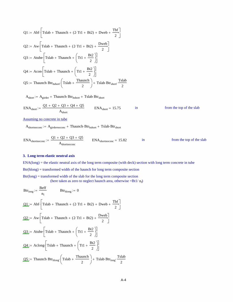
Q1 Abf Tslab Thaunch+ 2 Tt1⋅ Bt2+( )+ Dweb+Tbf
2+⎡⎢
⎣⎤⎥⎦
⋅:=
Q2 Aw Tslab Thaunch+ 2 Tt1⋅ Bt2+( )+Dweb
2+⎡⎢
⎣⎤⎥⎦
⋅:=
Q3 Atube Tslab Thaunch+ Tt1Bt22
+⎛⎜⎝
⎞⎟⎠
+⎡⎢⎣
⎤⎥⎦
⋅:=
Q4 Acon Tslab Thaunch+ Tt1Bt22
+⎛⎜⎝
⎞⎟⎠
+⎡⎢⎣
⎤⎥⎦
⋅:=
Q5 Thaunch Btrhshort⋅ TslabThaunch
2+⎛⎜
⎝⎞⎟⎠
⋅ Tslab Btrshort⋅Tslab
2⋅+:=
Ashort Agirder Thaunch Btrhshort⋅+ Tslab Btrshort⋅+:=
ENAshortQ1 Q2+ Q3+ Q4+ Q5+
Ashort:= ENAshort 15.75= in from the top of the slab
Assuming no concrete in tube
Ashortnoconc Agirdernoconc Thaunch Btrhshort⋅+ Tslab Btrshort⋅+:=
ENAshortnoconcQ1 Q2+ Q3+ Q5+
Ashortnoconc:= ENAshortnoconc 15.82= in from the top of the slab
3. Long term elastic neutral axis
ENA(long) = the elastic neutral axis of the long term composite (with deck) section with long term concrete in tube
Btr(hlong) = transformed width of the haunch for long term composite section
Btr(long) = transformed width of the slab for the long term composite section(here taken as zero to neglect haunch area, otherwise =Bt1/ nl)
BtrlongBeff
nl:= Btrhlong 0:=
Q1 Abf Tslab Thaunch+ 2 Tt1⋅ Bt2+( )+ Dweb+Tbf
2+⎡⎢
⎣⎤⎥⎦
⋅:=
Q2 Aw Tslab Thaunch+ 2 Tt1⋅ Bt2+( )+Dweb
2+⎡⎢
⎣⎤⎥⎦
⋅:=
Q3 Atube Tslab Thaunch+ Tt1Bt22
+⎛⎜⎝
⎞⎟⎠
+⎡⎢⎣
⎤⎥⎦
⋅:=
Q4 Aclong Tslab Thaunch+ Tt1Bt22
+⎛⎜⎝
⎞⎟⎠
+⎡⎢⎣
⎤⎥⎦
⋅:=
Q5 Thaunch Btrhlong⋅ TslabThaunch
2+⎛⎜
⎝⎞⎟⎠
⋅ Tslab Btrlong⋅Tslab
2⋅+:=
A-4

Along Agirderlong Thaunch Btrhlong⋅+ Tslab Btrlong⋅+:=
ENAlongQ1 Q2+ Q3+ Q4+ Q5+
Along:= ENAlong 23.27= in from the top of the concrete
Assuming no concrete in tube
Alongnoconc Atube Aw+ Abf+ Thaunch Btrhlong⋅+ Tslab Btrlong⋅+:=
ENAlongnoconcQ1 Q2+ Q3+ Q5+
Alongnoconc:= ENAlongnoconc 23.709= in from the top of the concrete
Calculate the moment of inertia for1. Steel section with short term concrete (n) in tube and with long term concrete(3n) in tube2. Short term composite (with deck) section (n) with short term concrete(n) in tube3. Long term composite (with deck) section (3*n) with long term concrete(3*n) in tube
1. Steel section moment of inertia
Ix(girder) = moment of inertia of the steel section with short term concrete in tube
Ix1112
Bbf⋅ Tbf 3⋅ Abf 2 Tt1⋅ Bt2+( ) Dweb+
Tbf2
+ ENAgirder−⎡⎢⎣
⎤⎥⎦
2⋅+:=
Ix2112
Tweb⋅ Dweb3⋅ Aw ENAgirder 2 Tt1⋅ Bt2+( )−
Dweb2
−⎡⎢⎣
⎤⎥⎦
2⋅+:=
Ix3112
Bt1⋅ Bt2 2 Tt1⋅+( )3⋅
112
Bt1 2 Tt2⋅−( )⋅ Bt23⋅−⎡⎢
⎣⎤⎥⎦
Atube ENAgirder Tt1Bt22
+⎛⎜⎝
⎞⎟⎠
−⎡⎢⎣
⎤⎥⎦
2⋅+:=
Ix4
112
Bt1 2 Tt2⋅−( )⋅ Bt23⋅
ns
Bt1 2 Tt2⋅−( ) Bt2⋅
nsENAgirder Tt1
Bt22
+⎛⎜⎝
⎞⎟⎠
−⎡⎢⎣
⎤⎥⎦
2⋅+:=
Ixgirder Ix1 Ix2+ Ix3+ Ix4+:= Ixgirder 15269= in4 <== short term concrete in tube
Ix(girderlong) = moment of inertia of the steel section with long term concrete in tube
Ix1lo112
Bbf⋅ Tbf 3⋅ Abf 2 Tt1⋅ Bt2+( ) Dweb+
Tbf2
+ ENAgirderlong−⎡⎢⎣
⎤⎥⎦
2⋅+:=
Ix2lo112
Tweb⋅ Dweb3⋅ Aw ENAgirderlong 2 Tt1⋅ Bt2+( )−
Dweb2
−⎡⎢⎣
⎤⎥⎦
2⋅+:=
A-5
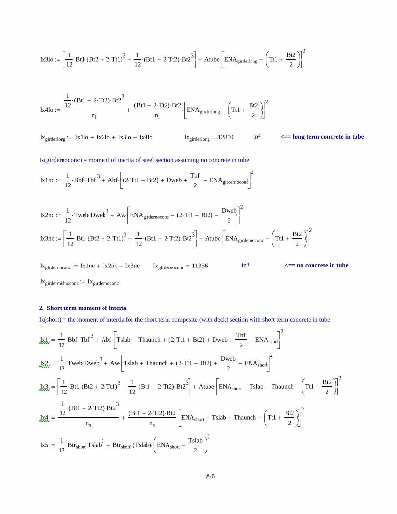
Ix3lo112
Bt1⋅ Bt2 2 Tt1⋅+( )3⋅
112
Bt1 2 Tt2⋅−( )⋅ Bt23⋅−⎡⎢
⎣⎤⎥⎦
Atube ENAgirderlong Tt1Bt22
+⎛⎜⎝
⎞⎟⎠
−⎡⎢⎣
⎤⎥⎦
2⋅+:=
Ix4lo
112
Bt1 2 Tt2⋅−( )⋅ Bt23⋅
nl
Bt1 2 Tt2⋅−( ) Bt2⋅
nlENAgirderlong Tt1
Bt22
+⎛⎜⎝
⎞⎟⎠
−⎡⎢⎣
⎤⎥⎦
2⋅+:=
Ixgirderlong Ix1lo Ix2lo+ Ix3lo+ Ix4lo+:= Ixgirderlong 12850= in4 <== long term concrete in tube
Ix(girdernoconc) = moment of inertia of steel section assuming no concrete in tube
Ix1nc112
Bbf⋅ Tbf 3⋅ Abf 2 Tt1⋅ Bt2+( ) Dweb+
Tbf2
+ ENAgirdernoconc−⎡⎢⎣
⎤⎥⎦
2⋅+:=
Ix2nc112
Tweb⋅ Dweb3⋅ Aw ENAgirdernoconc 2 Tt1⋅ Bt2+( )−
Dweb2
−⎡⎢⎣
⎤⎥⎦
2⋅+:=
Ix3nc112
Bt1⋅ Bt2 2 Tt1⋅+( )3⋅
112
Bt1 2 Tt2⋅−( )⋅ Bt23⋅−⎡⎢
⎣⎤⎥⎦
Atube ENAgirdernoconc Tt1Bt22
+⎛⎜⎝
⎞⎟⎠
−⎡⎢⎣
⎤⎥⎦
2⋅+:=
Ixgirdernoconc Ix1nc Ix2nc+ Ix3nc+:= Ixgirdernoconc 11356= in4 <== no concrete in tube
Ixgirdermidnoconc Ixgirdernoconc:=
2. Short term moment of interia
Ix(short) = the moment of intertia for the short term composite (with deck) section with short term concrete in tube
Ix1112
Bbf⋅ Tbf 3⋅ Abf Tslab Thaunch+ 2 Tt1⋅ Bt2+( )+ Dweb+
Tbf2
+ ENAshort−⎡⎢⎣
⎤⎥⎦
2⋅+:=
Ix2112
Tweb⋅ Dweb3⋅ Aw Tslab Thaunch+ 2 Tt1⋅ Bt2+( )+
Dweb2
+ ENAshort−⎡⎢⎣
⎤⎥⎦
2⋅+:=
Ix3112
Bt1⋅ Bt2 2 Tt1⋅+( )3⋅
112
Bt1 2 Tt2⋅−( )⋅ Bt23⋅−⎡⎢
⎣⎤⎥⎦
Atube ENAshort Tslab− Thaunch− Tt1Bt22
+⎛⎜⎝
⎞⎟⎠
−⎡⎢⎣
⎤⎥⎦
2⋅+:=
Ix4
112
Bt1 2 Tt2⋅−( )⋅ Bt23⋅
ns
Bt1 2 Tt2⋅−( ) Bt2⋅
nsENAshort Tslab− Thaunch− Tt1
Bt22
+⎛⎜⎝
⎞⎟⎠
−⎡⎢⎣
⎤⎥⎦
2⋅+:=
Ix5112
Btrshort⋅ Tslab3⋅ Btrshort Tslab( )⋅ ENAshort
Tslab2
−⎛⎜⎝
⎞⎟⎠
2⋅+:=
A-6
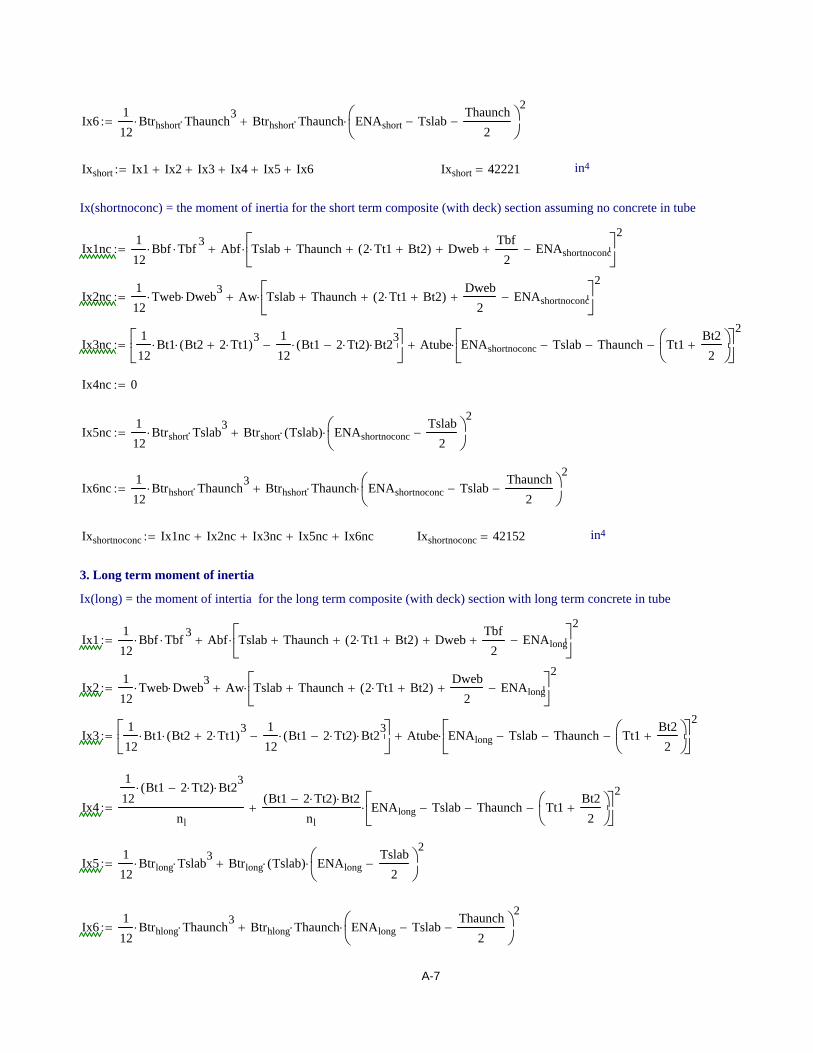
Ix6112
Btrhshort⋅ Thaunch3⋅ Btrhshort Thaunch⋅ ENAshort Tslab−
Thaunch2
−⎛⎜⎝
⎞⎟⎠
2⋅+:=
Ixshort Ix1 Ix2+ Ix3+ Ix4+ Ix5+ Ix6+:= Ixshort 42221= in4
Ix(shortnoconc) = the moment of inertia for the short term composite (with deck) section assuming no concrete in tube
Ix1nc112
Bbf⋅ Tbf 3⋅ Abf Tslab Thaunch+ 2 Tt1⋅ Bt2+( )+ Dweb+
Tbf2
+ ENAshortnoconc−⎡⎢⎣
⎤⎥⎦
2⋅+:=
Ix2nc112
Tweb⋅ Dweb3⋅ Aw Tslab Thaunch+ 2 Tt1⋅ Bt2+( )+
Dweb2
+ ENAshortnoconc−⎡⎢⎣
⎤⎥⎦
2⋅+:=
Ix3nc112
Bt1⋅ Bt2 2 Tt1⋅+( )3⋅
112
Bt1 2 Tt2⋅−( )⋅ Bt23⋅−⎡⎢
⎣⎤⎥⎦
Atube ENAshortnoconc Tslab− Thaunch− Tt1Bt22
+⎛⎜⎝
⎞⎟⎠
−⎡⎢⎣
⎤⎥⎦
2⋅+:=
Ix4nc 0:=
Ix5nc112
Btrshort⋅ Tslab3⋅ Btrshort Tslab( )⋅ ENAshortnoconc
Tslab2
−⎛⎜⎝
⎞⎟⎠
2⋅+:=
Ix6nc112
Btrhshort⋅ Thaunch3⋅ Btrhshort Thaunch⋅ ENAshortnoconc Tslab−
Thaunch2
−⎛⎜⎝
⎞⎟⎠
2⋅+:=
Ixshortnoconc Ix1nc Ix2nc+ Ix3nc+ Ix5nc+ Ix6nc+:= Ixshortnoconc 42152= in4
3. Long term moment of inertia
Ix(long) = the moment of intertia for the long term composite (with deck) section with long term concrete in tube
Ix1112
Bbf⋅ Tbf 3⋅ Abf Tslab Thaunch+ 2 Tt1⋅ Bt2+( )+ Dweb+
Tbf2
+ ENAlong−⎡⎢⎣
⎤⎥⎦
2⋅+:=
Ix2112
Tweb⋅ Dweb3⋅ Aw Tslab Thaunch+ 2 Tt1⋅ Bt2+( )+
Dweb2
+ ENAlong−⎡⎢⎣
⎤⎥⎦
2⋅+:=
Ix3112
Bt1⋅ Bt2 2 Tt1⋅+( )3⋅
112
Bt1 2 Tt2⋅−( )⋅ Bt23⋅−⎡⎢
⎣⎤⎥⎦
Atube ENAlong Tslab− Thaunch− Tt1Bt22
+⎛⎜⎝
⎞⎟⎠
−⎡⎢⎣
⎤⎥⎦
2⋅+:=
Ix4
112
Bt1 2 Tt2⋅−( )⋅ Bt23⋅
nl
Bt1 2 Tt2⋅−( ) Bt2⋅
nlENAlong Tslab− Thaunch− Tt1
Bt22
+⎛⎜⎝
⎞⎟⎠
−⎡⎢⎣
⎤⎥⎦
2⋅+:=
Ix5112
Btrlong⋅ Tslab3⋅ Btrlong Tslab( )⋅ ENAlong
Tslab2
−⎛⎜⎝
⎞⎟⎠
2⋅+:=
Ix6112
Btrhlong⋅ Thaunch3⋅ Btrhlong Thaunch⋅ ENAlong Tslab−
Thaunch2
−⎛⎜⎝
⎞⎟⎠
2⋅+:=
A-7
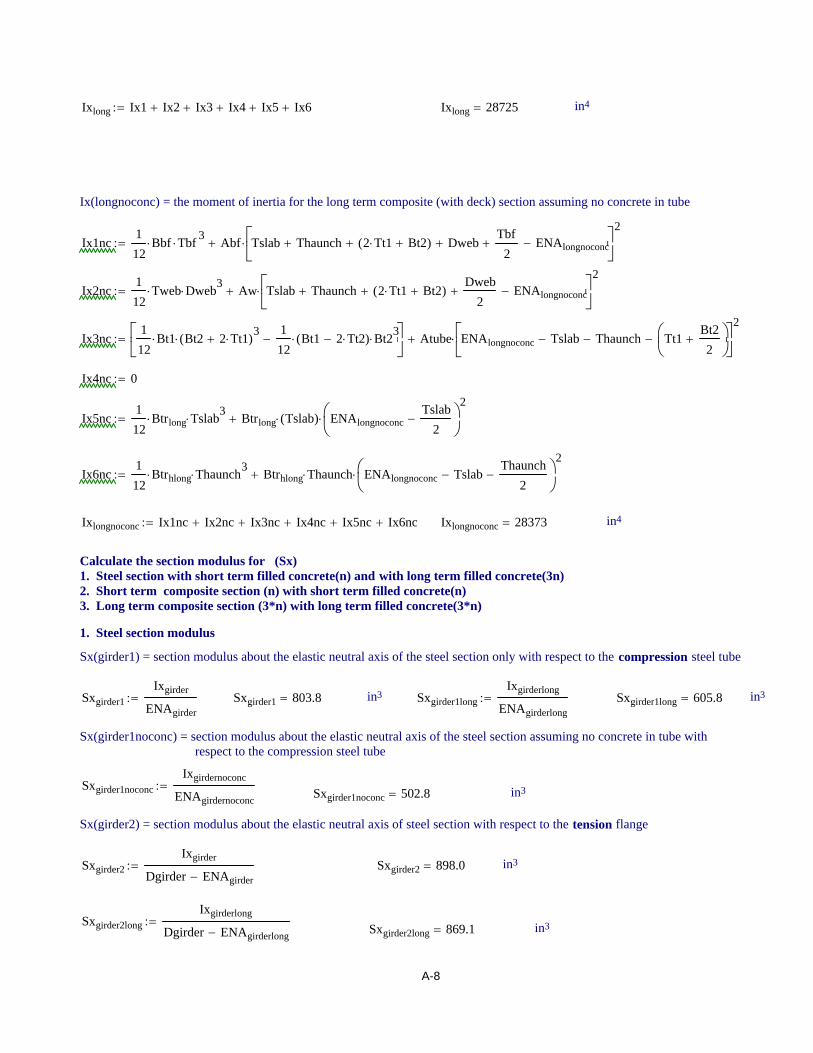
Ixlong Ix1 Ix2+ Ix3+ Ix4+ Ix5+ Ix6+:= Ixlong 28725= in4
Ix(longnoconc) = the moment of inertia for the long term composite (with deck) section assuming no concrete in tube
Ix1nc112
Bbf⋅ Tbf 3⋅ Abf Tslab Thaunch+ 2 Tt1⋅ Bt2+( )+ Dweb+
Tbf2
+ ENAlongnoconc−⎡⎢⎣
⎤⎥⎦
2⋅+:=
Ix2nc112
Tweb⋅ Dweb3⋅ Aw Tslab Thaunch+ 2 Tt1⋅ Bt2+( )+
Dweb2
+ ENAlongnoconc−⎡⎢⎣
⎤⎥⎦
2⋅+:=
Ix3nc112
Bt1⋅ Bt2 2 Tt1⋅+( )3⋅
112
Bt1 2 Tt2⋅−( )⋅ Bt23⋅−⎡⎢
⎣⎤⎥⎦
Atube ENAlongnoconc Tslab− Thaunch− Tt1Bt22
+⎛⎜⎝
⎞⎟⎠
−⎡⎢⎣
⎤⎥⎦
2⋅+:=
Ix4nc 0:=
Ix5nc112
Btrlong⋅ Tslab3⋅ Btrlong Tslab( )⋅ ENAlongnoconc
Tslab2
−⎛⎜⎝
⎞⎟⎠
2⋅+:=
Ix6nc112
Btrhlong⋅ Thaunch3⋅ Btrhlong Thaunch⋅ ENAlongnoconc Tslab−
Thaunch2
−⎛⎜⎝
⎞⎟⎠
2⋅+:=
Ixlongnoconc Ix1nc Ix2nc+ Ix3nc+ Ix4nc+ Ix5nc+ Ix6nc+:= Ixlongnoconc 28373= in4
Calculate the section modulus for (Sx)1. Steel section with short term filled concrete(n) and with long term filled concrete(3n)2. Short term composite section (n) with short term filled concrete(n)3. Long term composite section (3*n) with long term filled concrete(3*n)
1. Steel section modulus
Sx(girder1) = section modulus about the elastic neutral axis of the steel section only with respect to the compression steel tube
Sxgirder1Ixgirder
ENAgirder:= Sxgirder1 803.8= in3 Sxgirder1long
Ixgirderlong
ENAgirderlong:= Sxgirder1long 605.8= in3
Sx(girder1noconc) = section modulus about the elastic neutral axis of the steel section assuming no concrete in tube with respect to the compression steel tube
Sxgirder1noconcIxgirdernoconc
ENAgirdernoconc:= Sxgirder1noconc 502.8= in3
Sx(girder2) = section modulus about the elastic neutral axis of steel section with respect to the tension flange
Sxgirder2Ixgirder
Dgirder ENAgirder−:= Sxgirder2 898.0= in3
Sxgirder2longIxgirderlong
Dgirder ENAgirderlong−:= Sxgirder2long 869.1= in3
A-8

Sx(girder2noconc) = section modulus about the elastic neutral axis of the steel section assuming no concrete in tube with respect to the tension flange
Sxgirder2noconcIxgirdernoconc
Dgirder ENAgirdernoconc−:= Sxgirder2noconc 846.743= in3
2. Short term section modulus
Sx(short1) = the section modulus about the elastic neutral axis for the compression steel tube of the short term composite section
Sxshort1Ixshort
ENAshort Thaunch− Tslab−:= Sxshort1 8896= in3
Sx(short1noconc) = the section modulus about the elastic neutral axis for the compression steel tube of the short term composite section assuming there is no concrete in the tube
Sxshort1noconcIxshortnoconc
ENAshortnoconc Thaunch− Tslab−:= Sxshort1noconc 8749.9= in3
Sx(short2) = the section modulus about the elastic neutral axis for the tension flange of the short term composite section
Sxshort2Ixshort
Dtotal ENAshort−:= Sxshort2 1350.9=
Sx(short2noconc) = the section modulus about the elastic neutral axis for the tension flange of the short term composite section assuming there is no concrete in the tube
Sxshort2noconcIxshortnoconc
Dtotal ENAshortnoconc−:= Sxshort2noconc 1351.8= in3
3. Long term section modulus
Sx(long1) = the section modulus about the elastic neutral axis for the compression steel tube of the long term composite section
Sxlong1Ixlong
ENAlong Thaunch− Tslab−:= Sxlong1 2341.3= in3
Sx(long1noconc) = the section modulus about the elastic neutral axis for the compression steel tube of the long term composite section assuming there is no concrete in the tube
Sxlong1noconcIxlongnoconc
ENAlongnoconc Thaunch− Tslab−:= Sxlong1noconc 2232.6= in3
Sx(long2) = the section modulus about the elastic neutral axis for the tension flange of the long term composite section
Sxlong2Ixlong
Dtotal ENAlong−:= Sxlong2 1210.5= in3
Sx(long2noconc) = the section modulus about the elastic neutral axis for the tension flange of the long term composite section assuming there is no concrete in the tube
A-9
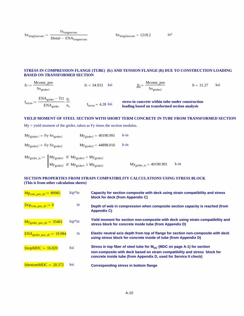
Sxlong2noconcIxlongnoconc
Dtotal ENAlongnoconc−:= Sxlong2noconc 1218.2= in3
STRESS IN COMPRESSION FLANGE (TUBE) (fc) AND TENSION FLANGE (ft) DUE TO CONSTRUCTION LOADINGBASED ON TRANSFORMED SECTION
fcMconst_pos
Sxgirder1:= fc 34.933= ksi ft
Mconst_posSxgirder2
:= ft 31.27= ksi
finconENAgirder Tt1−
ENAgirder
fcns
⋅:= stress in concrete within tube under constructionloading based on transformed section analysisfincon 4.28= ksi
YIELD MOMENT OF STEEL SECTION WITH SHORT TERM CONCRETE IN TUBE FROM TRANSFORMED SECTION
My = yield moment of the girder, taken as Fy times the section modulus.
Mygirder1 Fy Sxgirder1⋅:= Mygirder1 40190.991= k-in
Mygirder2 Fy Sxgirder2⋅:= Mygirder2 44898.016= k-in
Mygirder_ts Mygirder1 Mygirder1 Mygirder2<if
Mygirder2 Mygirder1 Mygirder2≥if
:=
Mygirder_ts 40190.991= k-in
SECTION PROPERTIES FROM STRAIN COMPATIBILITY CALCULATIONS USING STRESS BLOCK(This is from other calculation sheets)
Mpcom_pos_sb 80985:= kip*in Capacity for section composite with deck using strain compatibility and stressblock for deck (from Appendix C)
Depth of web in compression when composite section capacity is reached (fromAppendix C)
Yield moment for section non-composite with deck using strain compatibility andstress block for concrete inside tube (from Appendix D)
Elastic neutral axis depth from top of flange for section non-composite with deckusing stress block for concrete inside of tube (from Appendix D)
Stress in top fiber of steel tube for MDC (MDC on page A-1) for sectionnon-composite with deck based on strain compatibility and stress block forconcrete inside tube (from Appendix D, used for Service II check)
Corresponding stress in bottom flange
Dcpcom_pos_sb 0:= in
Mygirder_pos_sb 35401:= kip*in
ENAgirder_pos_sb 19.984:= in
fstopMDC 16.820:= ksi
fsbottomMDC 20.372:= ksi
A-10

CONSTRUCTION LOADING CHECK FOR FLEXURE
Yield moment of the steel sectionMygirder_ts 40191= transformed section My
Mygirder_pos Mygirder_ts Mygirder_ts Mygirder_pos_sb<if
Mygirder_pos_sb Mygirder_ts Mygirder_pos_sb≥if
:= Mygirder_pos_sb 35401= strain compatibility (stress block) My
Mygirder_pos 35401= k-in
Calculate depth of web in compression for construction, Dc
Dc_ts ENAgirder 2Tt1 Bt2+( )−:= Dc_ts 11.00= in
Dc_pos_sb ENAgirder_pos_sb 2Tt1 Bt2+( )−:= Dc_pos_sb 11.98= in
Dc_pos Dc_ts Mygirder_ts Mygirder_pos_sb<if
Dc_pos_sb Mygirder_ts Mygirder_pos_sb≥if
:=
Dc_pos 11.98= in
Web Slenderness Limit for "stocky web"
AtfBt2 Bt1 2 Tt2⋅−( )⋅
nsAtube+:= Atf 31.258= in2 Abf 27= in2
λb 5.76 Atf Abf≥if
4.64 Atf Abf<if
:=λb 5.76=
Aw 2Dc_posTweb
⋅:= Fw λbEFy
⋅:= Ratioweb_stockyAw
Fw:=
if Ratioweb_stocky 0.346= < 1 then this section has stocky web
Web Slenderness Limit to minimize web distortion
Aw_distDwebTweb
:= Fw_dist 11EFy
⎛⎜⎝
⎞⎟⎠
1
3⋅:= Ratioweb_dist
Aw_dist
Fw_dist:=
if Ratioweb_dist 0.578= < 1 then this section is ok
General Cross Section Properties
Iyc112
Bt2 2 Tt1⋅+( )⋅ Bt13⋅
112
Bt2⋅ Bt1 2 Tt2⋅−( )3⋅−
112
Bt2⋅ Bt1 2 Tt2⋅−( )3⋅
ns+:= Iyc 855.8= in4
Iyt112
Tbf⋅ Bbf 3⋅:= Iyt 729.0= in4
Iy112
Dweb⋅ Tweb3⋅ Iyt+ Iyc+:= Iy 1585.1= in4
A-11

ryIyc Iyt+
Agirder:= ry 4.71= in
Torsional Properties
KTDweb Tweb3
⋅
3Bbf Tbf 3
⋅
3+
β Bt1 2 Tt2⋅−( )⋅ Bt23⋅
ns+
2 Tt2⋅ Tt1⋅ Bt1 Tt2−( )2⋅ Bt2 Tt1+( )2
⋅
Bt1 Tt2−( ) Tt2⋅ Bt2 Tt1+( ) Tt1⋅++:= KT 665.9= in4
Calculate the nominal moment capacity for lateral torsional buckling (LTB)For demonstration purposes, calculate the nominal LTB capacity twice: (1) without the midspan cross frame and (2) including the midspan cross frame. Normally the calculation would be done only once for the appropriate bracing condition
1. Here the calculation is performed for no interior bracing within the span. The nominal LTB flexural strength iscalculated assuming the entire span is the unbraced length with fixed brace points at the ends of the span (known as theideal flexural strength).
For the parabolic moment diagram with M=0 at the ends, Cb = 1.0 by 2004 AASHTO. Here use more accurate Cb=1.136
Lb0 L:= Lb0 1200= inCb0 1.136:=
Using equations for ideal design flexural strength
Lb Lb0:= Cb Cb0:=
Critical elastic LTB moment
Mcrπ E⋅Lb
ry
0.385 KT⋅ Agirder⋅2.467 Dgirder2
⋅ Agirder2
⋅
Lbry
⎛⎜⎝
⎞⎟⎠
2+⋅:= Mcr 48725.6= k-in
Cross section moment capacity
Ms Mygirder_pos:= Ms 35401.0= k-in
Strength reduction factor to account for LTB
αs_var 0.8MsMcr
⎛⎜⎝
⎞⎟⎠
22.2+
MsMcr
−⎡⎢⎣
⎤⎥⎦
⋅:= αs αs_var αs_var 1.0≤if
1.0 otherwise
:= αs 0.74=
Design flexural strength accounting for LTB
Md_var Cb αs⋅ Ms⋅:= Md0 Md_var Md_var Ms≤if
Ms otherwise
:= Md0 29762.2= k-in
A-12

2. Here, the calculation is performed for one interior brace at the midspan of the span. So the torsionally braced nominalflexural strength is calculated assuming the unbraced length is one half the span.
First, the ideal design flexural strength that corresponds to LTB between the brace points is calculated (i.e., using theunbraced length equal to 1/2 of the span and the appropriate Cb). This is upper bound on the nominal LTB flexural strength.
For the parabolic moment diagram with M=0 at one end and Mmax at the other end, Cb is calculated according to 2004AASHTO as follows (using moment instead of stress since section is constant).
Lb1L2
:= Lb1 600= in
Determine M1 and M2 (maximum moment moment at midspan brace). Here M0 = 0 (the moment at theend of the span, and Mmid = the moment at the quarter point, which is 3/4 of the midspan moment
M0 0:= Mmid 0.75 Mconst_pos⋅:= kip-in M2 Mconst_pos:= M2 28080= kip-in
M1 2 Mmid⋅ M2−:= M1 14040= > M0 0= OK
Determine Cb from M1 and M2
Cb1 1.75 1.05M1M2
⎛⎜⎝
⎞⎟⎠
⋅− 0.3M1M2
⎛⎜⎝
⎞⎟⎠
2⋅+:= Cb1 1.3=
Ideal design flexural strength for LTB between braces calculated as above with the following Lb and Cb
Lb Lb1:= Cb Cb1:=
Mcrπ E⋅Lb
ry
0.385 KT⋅ Agirder⋅2.467 Dgirder2
⋅ Agirder2
⋅
Lbry
⎛⎜⎝
⎞⎟⎠
2+⋅:= Mcr 99410.5= k-in
Ms Mygirder_pos:= Ms 35401.0= k-in
αs_var 0.8MsMcr
⎛⎜⎝
⎞⎟⎠
22.2+
MsMcr
−⎡⎢⎣
⎤⎥⎦
⋅:= αs αs_var αs_var 1.0≤if
1.0 otherwise
:= αs 0.935=
Md_var Cb αs⋅ Ms⋅:= Md1 Md_var Md_var Ms≤if
Ms otherwise
:= Md1 35401= k-in
Then, the design flexural strength for the torsionally braced CFTFGs is calculated.
Consider the entire span length and corresponding moment diagram. For the parabolic moment diagram with M=0 at the ends,Cb = 1.0 according to 2004 AASHTO. Here use more accurate Cb=1.136
Cbu 1.136:=Critical elastic LTB moment for girder without interior bracing in span (note Lb=L in formula)
Mcr_ubrπ E⋅L
ry
0.385 KT⋅ Agirder⋅2.467 Dgirder2
⋅ Agirder2
⋅
Lry
⎛⎜⎝
⎞⎟⎠
2+⋅:= Mcr_ubr 48725.6= k-in
A-13

Critical moment including the bracing effect - required input regarding bracing properties
nb 1:= Number of interior bracing per span
Ib 1170:= in4 Moment of inertia of bracing member about strong axis
N 1:= in Contact length of torsional brace
ts 1.5:= in stiffener thickness
bs 16:= in stiffener width
Critical moment including the bracing effect - calculate Ieff, β, etc.
c Dc_pos Tt1+Bt22
+:= c 15.98= in t Dgirder Dc_pos− 2 Tt1⋅− Bt2−Tbf
2−:= t 15.27= in
Ieff Iyctc
Iyt⋅+:= Ieff 1552.0= Effective vertical axis moment of inertia
hBt22
Tt1+ Dweb+Tbf
2+:= h 31.25= Distance between flange centroids
βb6 E⋅ Ib⋅
s:= βb 2.006 106
×=
βg24 ng 1−( )2
⋅
ng
s2 E⋅ Ixgirder⋅
L3⋅:= βg 1.426 105
×=
βsec 3.3Eh
⋅N 1.5 h⋅+( ) Tweb3
⋅
12ts bs3
⋅
12+
⎡⎢⎣
⎤⎥⎦
⋅:= βsec 1.569 106×=
βT 1:= Determine βT
eq βT( )1
βb1
βsec+
1βg
+1
βT−:= βT root eq βT( ) βT, ( ):= βT 1.227 105
×=
Critical moment including the bracing effect.
MbrβT E⋅ Ieff⋅ nb⋅
1.2 L⋅:= Mbr 61927= k-in
Critical elastic LTB moment including torsional brace effect
Cbb Cb1:= Cbb 1.3=
Mcr_br Mcr_ubr2 Cbb2
Cbu2Mbr2⋅+:= Mcr_br 86002= k-in
Strength reduction factor for torsionally braced girder
αs 0.935=αs_br_var 0.8
MsMcr_br
⎛⎜⎝
⎞⎟⎠
22.2+
MsMcr_br
−⎡⎢⎣
⎤⎥⎦
⋅:= αs_br αs_br_var αs_br_var 1.0≤if
1.0 otherwise
:=
A-14
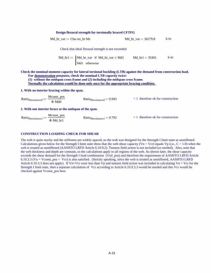
Design flexural strength for torsionally braced CFTFG
Md_br_var Cbu αs_br⋅ Ms⋅:= Md_br_var 36279.8= k-in
Check that ideal flexural strength is not exceeded
Md_br1 Md_br_var Md_br_var Md1≤if
Md1 otherwise
:= Md_br1 35401= k-in
Check the nominal moment capacity for lateral torsional buckling (LTB) against the demand from construction load.For demonstration purposes, check the nominal LTB capacity twice: (1) without the midspan cross frame and (2) including the midspan cross frame. Normally the calculation would be done only once for the appropriate bracing condition
1. With no interior bracing within the span.
Ratioltbresistance0Mconst_pos
Φ Md0⋅:= Ratioltbresistance0 0.943= < 1 therefore ok for construction
2. With one interior brace at the midspan of the span.
Ratioltbresistance1Mconst_posΦ Md_br1⋅
:= Ratioltbresistance1 0.793= < 1 therefore ok for construction
CONSTRUCTION LOADING CHECK FOR SHEAR
The web is quite stocky and the stiffeners are widely spaced, so the web was designed for the Strength I limit state as unstiffened.Calculations given below for the Strength I limit state show that the web shear capacity (Vn = Vcr) equals Vp (i.e., C = 1.0) when theweb is treated as unstiffened (AASHTO LRFD Article 6.10.9.2). Tension field action is not included (or needed). Also, note thatthe web thickness and depth are constant, so the calculations apply to all regions of the web. As shown later, the shear capacityexceeds the shear demand for the Strength I load combination (VstI_pos) and therefore the requirement of AASHTO LRFD Article6.10.3.3 (Vu = Vconst_pos < Vcr) is also satisfied. (Strictly speaking, since the web is treated as unstiffened, AASHTO LRFDArticle 6.10.3.3 does not apply). If Vn=Vcr were less than Vp and tension field action was included in calculating Vn = Vcr for theStrength I limit state, then a separate calculation of Vcr according to Article 6.10.9.3.3 would be needed and this Vcr would bechecked against Vconst_pos here.
A-15
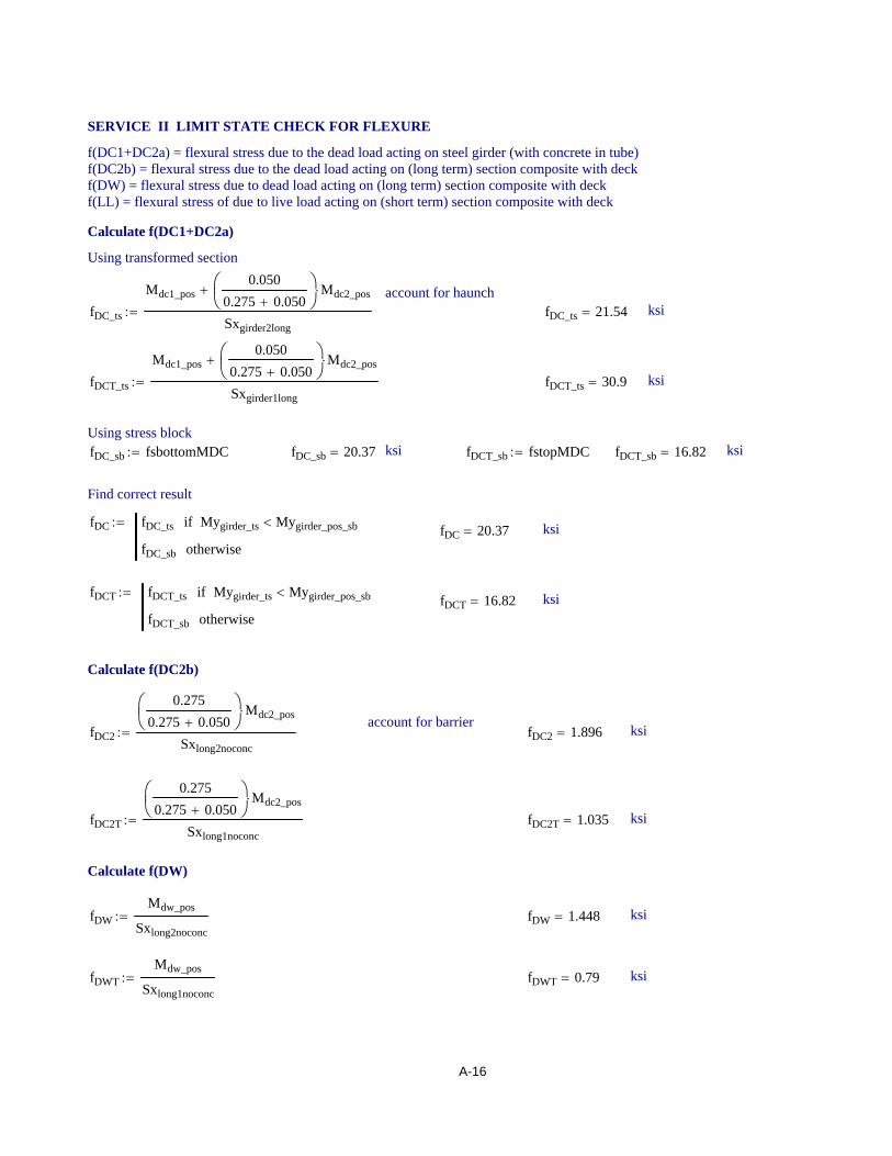
SERVICE II LIMIT STATE CHECK FOR FLEXURE
f(DC1+DC2a) = flexural stress due to the dead load acting on steel girder (with concrete in tube)f(DC2b) = flexural stress due to the dead load acting on (long term) section composite with deckf(DW) = flexural stress due to dead load acting on (long term) section composite with deckf(LL) = flexural stress of due to live load acting on (short term) section composite with deck
Calculate f(DC1+DC2a)
Using transformed section
account for haunchfDC_ts
Mdc1_pos0.050
0.275 0.050+⎛⎜⎝
⎞⎟⎠
Mdc2_pos⋅+
Sxgirder2long:= fDC_ts 21.54= ksi
fDCT_ts
Mdc1_pos0.050
0.275 0.050+⎛⎜⎝
⎞⎟⎠
Mdc2_pos⋅+
Sxgirder1long:= fDCT_ts 30.9= ksi
Using stress blockfDC_sb fsbottomMDC:= fDC_sb 20.37= ksi fDCT_sb fstopMDC:= fDCT_sb 16.82= ksi
Find correct result
fDC fDC_ts Mygirder_ts Mygirder_pos_sb<if
fDC_sb otherwise
:= fDC 20.37= ksi
fDCT fDCT_ts Mygirder_ts Mygirder_pos_sb<if
fDCT_sb otherwise
:= fDCT 16.82= ksi
Calculate f(DC2b)
account for barrierfDC2
0.2750.275 0.050+
⎛⎜⎝
⎞⎟⎠
Mdc2_pos⋅
Sxlong2noconc:= fDC2 1.896= ksi
fDC2T
0.2750.275 0.050+
⎛⎜⎝
⎞⎟⎠
Mdc2_pos⋅
Sxlong1noconc:= fDC2T 1.035= ksi
Calculate f(DW)
fDWMdw_pos
Sxlong2noconc:= fDW 1.448= ksi
fDWTMdw_pos
Sxlong1noconc:= fDWT 0.79= ksi
A-16
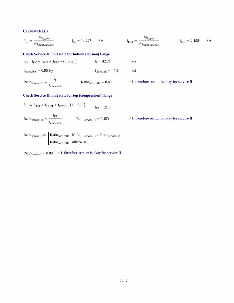
Calculate f(LL)
fLLMll_pos
Sxshort2noconc:= fLL 14.227= ksi fLLT
Mll_pos
Sxshort1noconc:= fLLT 2.198= ksi
Check Service II limit state for bottom (tension) flange
fF fDC fDC2+ fDW+ 1.3 fLL⋅( )+:= fF 42.21= ksi
fallowable 0.95 Fy⋅:= fallowable 47.5= ksi
RatioserviceII2fF
fallowable:= RatioserviceII2 0.89= < 1 therefore section is okay for service II
Check Service II limit state for top (compression) flange
fFT fDCT fDC2T+ fDWT+ 1.3 fLLT⋅( )+:= fFT 21.5=
RatioserviceII1fFT
fallowable:= RatioserviceII1 0.453= < 1 therefore section is okay for service II
RatioserviceII RatioserviceII1 RatioserviceII1 RatioserviceII2>if
RatioserviceII2 otherwise
:=
RatioserviceII 0.89= < 1 therefore section is okay for service II
A-17

CHECK STRENGTH I LIMIT STATE FOR FLEXURE
Since Dcpcom_pos_sb 0= The depth of the web in compression at the plastic moment is zero.
The web-slenderness requirement is satisfied. Therefore, the section qualifies as a compact section. The ductilitycheck is not required because the plastic moment is determined through strain compatibility.
Check the section capacity against the upper limit on section capacity for continuous spans
Calculate My according to AASHTO 2004
Bottom (tension) flange
MAD Sxshort2noconc Fy 1.25 fDC fDC2+( )⋅ 1.5 fDW⋅+⎡⎣ ⎤⎦−⎡⎣ ⎤⎦⋅:= MAD 27025.4= k-in
My_bf_st MAD 1.25 Mdc1_pos Mdc2_pos+( )+ 1.5 Mdw_pos⋅+:= My_bf_st 55958.9= k-in
Top (compression) flange
MADT Sxshort1noconc Fy 1.25 fDCT fDC2T+( )⋅ 1.5 fDWT⋅+⎡⎣ ⎤⎦−⎡⎣ ⎤⎦⋅:= MADT 231840.8= k-in
My_tf_st MADT 1.25 Mdc1_pos Mdc2_pos+( )+ 1.5 Mdw_pos⋅+:= My_tf_st 260774.3= k-in
Upper limit on section capacity according to AASHTO 2004
Mn_pos_max 1.3 Rh⋅ min My_bf_st My_tf_st, ( )⋅:= Mn_pos_max 72746.6= k-in
Section capacity.
Mn min Mn_pos_max Mpcom_pos_sb, ( ):= Mn 72746.6= k-in
Check Strength I limit state for flexure
RatioIflexureMstI_pos
Φ Mn⋅:= RatioIflexure 0.8174= < 1 therefore ok
A-18
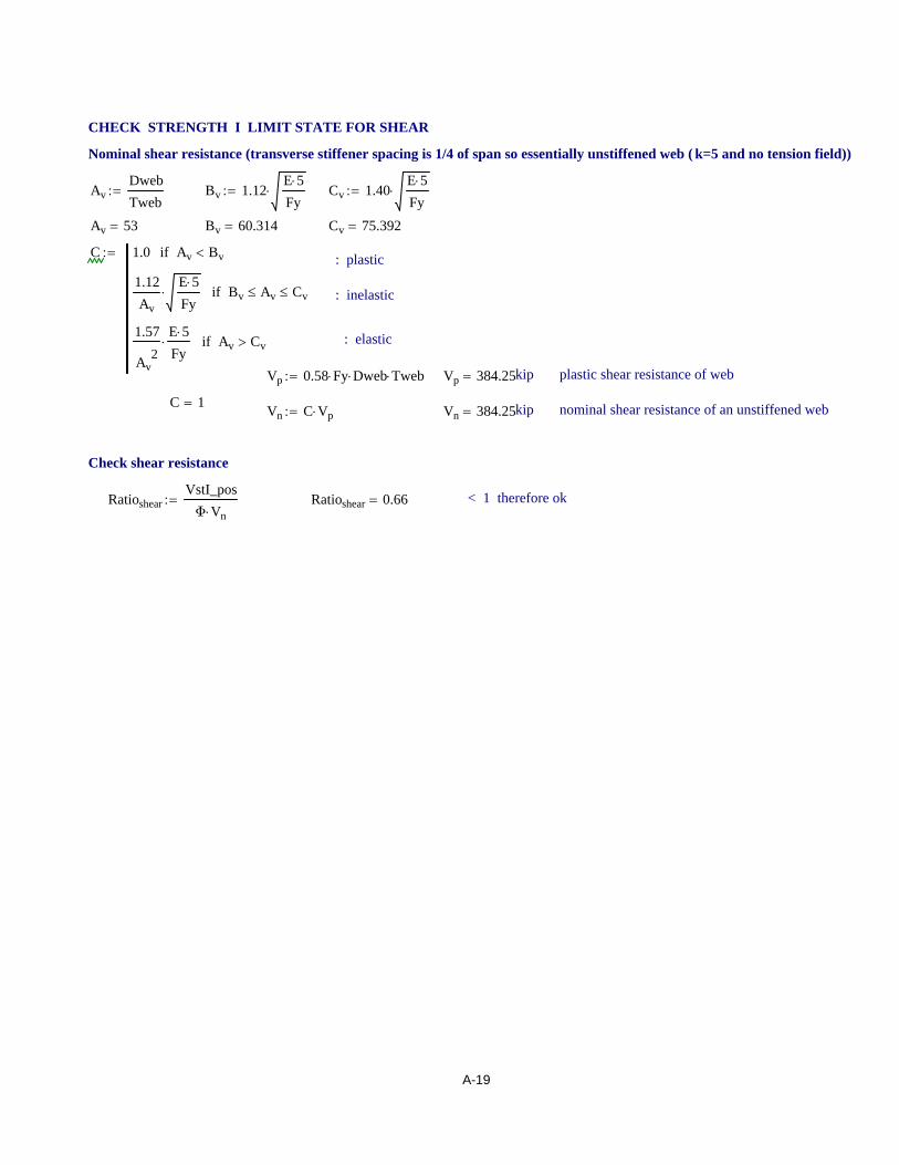
CHECK STRENGTH I LIMIT STATE FOR SHEAR
Nominal shear resistance (transverse stiffener spacing is 1/4 of span so essentially unstiffened web ( k=5 and no tension field))
AvDwebTweb
:= Bv 1.12E 5⋅Fy
⋅:= Cv 1.40E 5⋅Fy
⋅:=
Av 53= Bv 60.314= Cv 75.392=
C 1.0 Av Bv<if
1.12Av
E 5⋅Fy
⋅ Bv Av≤ Cv≤if
1.57
Av2
E 5⋅Fy
⋅ Av Cv>if
:= : plastic
: inelastic
: elastic
Vp 0.58 Fy⋅ Dweb⋅ Tweb⋅:= Vp 384.25= kip plastic shear resistance of web
C 1= Vn C Vp⋅:= Vn 384.25= kip nominal shear resistance of an unstiffened web
Check shear resistance
RatioshearVstI_pos
Φ Vn⋅:= Ratioshear 0.66= < 1 therefore ok
A-19
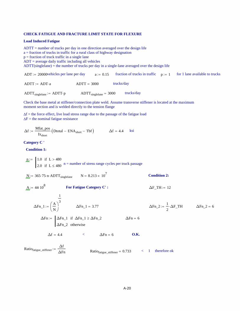
CHECK FATIGUE AND FRACTURE LIMIT STATE FOR FLEXURE
Load Induced Fatigue
ADTT = number of trucks per day in one direction averaged over the design lifea = fraction of trucks in traffic for a rural class of highway designationp = fraction of truck traffic in a single laneADT = average daily traffic including all vehiclesADTT(singlelane) = the number of trucks per day in a single-lane averaged over the design life
ADT 20000:= vehicles per lane per day a 0.15:= fraction of trucks in traffic p 1:= for 1 lane available to trucks
ADTT ADT a⋅:= ADTT 3000= trucks/day
ADTTsinglelane ADTT p⋅:= ADTTsinglelane 3000= trucks/day
Check the base metal at stiffener/connection plate weld. Assume transverse stiffener is located at the maximummoment section and is welded directly to the tension flange
Δf = the force effect, live load stress range due to the passage of the fatigue loadΔF = the nominal fatigue resistance
ΔfMfat_pos
IxshortDtotal ENAshort− Tbf−( )⋅:= Δf 4.4= ksi
Category C '
Condition 1:
n 1.0 L 480>if
2.0 L 480≤if
:=n = number of stress range cycles per truck passage
N 365 75⋅ n⋅ ADTTsinglelane⋅:= N 8.213 107×= Condition 2:
A 44 108⋅:= For Fatigue Category C' : ΔF_TH 12:=
ΔFn_1AN
⎛⎜⎝
⎞⎟⎠
1
3:= ΔFn_1 3.77= ΔFn_2
12
ΔF_TH⋅:= ΔFn_2 6=
ΔFn ΔFn_1 ΔFn_1 ΔFn_2≥if
ΔFn_2 otherwise
:= ΔFn 6=
Δf 4.4= < ΔFn 6= O.K.
Ratiofatigue_stiffenerΔf
ΔFn:= Ratiofatigue_stiffener 0.733= < 1 therefore ok
A-20
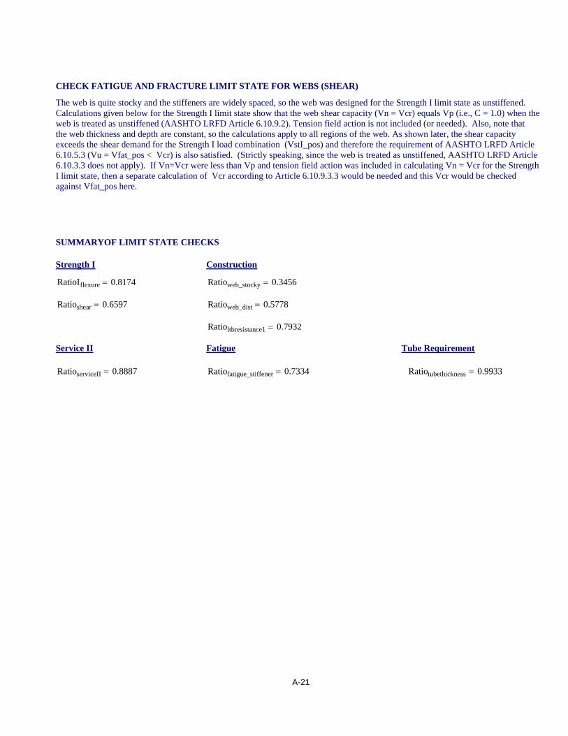
CHECK FATIGUE AND FRACTURE LIMIT STATE FOR WEBS (SHEAR)
The web is quite stocky and the stiffeners are widely spaced, so the web was designed for the Strength I limit state as unstiffened.Calculations given below for the Strength I limit state show that the web shear capacity (Vn = Vcr) equals Vp (i.e., C = 1.0) when theweb is treated as unstiffened (AASHTO LRFD Article 6.10.9.2). Tension field action is not included (or needed). Also, note thatthe web thickness and depth are constant, so the calculations apply to all regions of the web. As shown later, the shear capacityexceeds the shear demand for the Strength I load combination (VstI_pos) and therefore the requirement of AASHTO LRFD Article6.10.5.3 (Vu = Vfat_pos < Vcr) is also satisfied. (Strictly speaking, since the web is treated as unstiffened, AASHTO LRFD Article6.10.3.3 does not apply). If Vn=Vcr were less than Vp and tension field action was included in calculating Vn = Vcr for the StrengthI limit state, then a separate calculation of Vcr according to Article 6.10.9.3.3 would be needed and this Vcr would be checkedagainst Vfat_pos here.
SUMMARYOF LIMIT STATE CHECKS
Strength I Construction
RatioIflexure 0.8174= Ratioweb_stocky 0.3456=
Ratioshear 0.6597= Ratioweb_dist 0.5778=
Ratioltbresistance1 0.7932=
Service II Fatigue Tube Requirement
RatioserviceII 0.8887= Ratiofatigue_stiffener 0.7334= Ratiotubethickness 0.9933=
A-21

Appendix B. Pier Section and Negative Moment Region Preliminary Design
Part 1. Negative Moment Region Preliminary Design
I. Cross Section Information (yellow highlight indicates input data)
16x8x0.375
26.5x0.5
18x1.5(unit: in)
Yield strength: Fy 50:= ksi
Tensile strength: Fu 65:= ksi
Tube horizontal plate thickness: Tt138
:= in Note that tube has 5 in.cut out on each sidewall for splice access.Tube vertical plate thickness: Tt2
38
:= in
Tube horizontal plate width: Bt1 16:= in
Tube vertical plate width: Bt2 7.25:= in
Tube depth: Dtube Bt2 2 Tt2⋅+:= Dtube 8.00= in
Bottom flange thickness: Tbf 1.5:= in
Post-tensioning in Deck (per girder)Bottom flange width: Bbf 18:= in Number of Strands: Nstr 30:=
Web thickness: Tweb 0.5:= in Area of Strands: Astr Nstr 0.217⋅:= in2
Web depth: Dweb 26.5:= in Astr 6.51= in2
Girder depth: Dgird Dtube Dweb+ Tbf+:= Dgird 36.00= inFu_str 270:= ksi
Strand Strength:Fy_str 0.9 Fu_str⋅:=Deck Thickness: Tslab 8:= inFy_str 243= ksiHaunch Thickness: Thaunch 3:= in
Deck Concrete Strength: fcprime 4:= ksiDeck Width: W 376.5:= inShort-term Modular Ratio: ns 8:=Span Length: L 1200:= in
Girder Spacing: s 101.5:= in Number of Girders: ng 4:=
Overhang (from girder centerline): se 36:= in
Girder Areas
Abf Bbf Tbf⋅:= Abf 27= in2
Atube 2 Tt1⋅ Bt1⋅ 2 Tt2⋅ Bt2⋅+ 2 0.375⋅ 5⋅−:= Atube 13.69= in2 Includes cut-out
Aw Dweb Tweb⋅:= Aw 13.25= in2
Agird Aw Atube+ Abf+:= Agird 53.94= in2
B-1

EFFECTIVE WIDTH OF SLAB (INTERIOR GIRDER)
beff1L4
:= beff1 300.00= beff2 s:= beff2 101.50= beff3 12 Tslab⋅Bt12
+:= beff3 104.00=
The smallest beff governsBeffi beff1 beff1 beff2≤ beff1 beff3≤∧if
beff2 beff2 beff1≤ beff2 beff3≤∧if
beff3 otherwise
:=
Beffi 101.50= in
EFFECTIVE WIDTH OF SLAB (EXTERIOR GIRDER)
beff4s2
⎛⎜⎝
⎞⎟⎠
se+:= beff4 86.75=
The smallest beff governsBeffe beff1 beff1 beff2≤ beff1 beff3≤∧if
beff4 beff4 beff1≤ beff4 beff3≤∧if
beff3 otherwise
:=
Beffe 86.75= in
SELECT EFFECTIVE WIDTH OF SLAB (use Beffi for interior girder, Beffe for exterior girder, or minimum)
Beff min Beffe Beffi, ( ):= Beff 86.75= Note: here the minimum is used, which is for an exterior girder.
Deck Transformed Cross Section Area:
Ad_trBeff Tslab⋅ Astr−
nsAstr+:= Ad_tr 92.45= in2
SECTION PROPERTIES
Calculate the elastic neutral axis for steel girder section with post-tensioning steel in thedeck. The concrete in the tube is neglected since it is not present at the pier centerlinesection where the splice is made. The tube cross section includes the cut out for the splice.The reference line is taken at the bottom of the bottom flange.
Agird_pt Agird Astr+:= Agird_pt 60.45= in2
ENAgird_pt
Astr Dgird Thaunch+Tslab
2+⎛⎜
⎝⎞⎟⎠
⋅ Atube Tbf Dweb+Dtube
2+⎛⎜
⎝⎞⎟⎠
⋅+ Aw TbfDweb
2+⎛⎜
⎝⎞⎟⎠
⋅+ AbfTbf
2⎛⎜⎝
⎞⎟⎠
⋅+
Agird_pt:=
ENAgird_pt 15.45= in from the bottom of the girder
Calculate the corresponding moment of inertia for steel girder section with post-tensioning steel.
Ix1112
Bbf⋅ Tbf 3⋅ Abf
Tbf2
ENAgird_pt−⎛⎜⎝
⎞⎟⎠
2⋅+:=
Ix2112
Tweb⋅ Dweb3⋅ Aw Tbf
Dweb2
+ ENAgird_pt−⎛⎜⎝
⎞⎟⎠
2⋅+:=
B-2
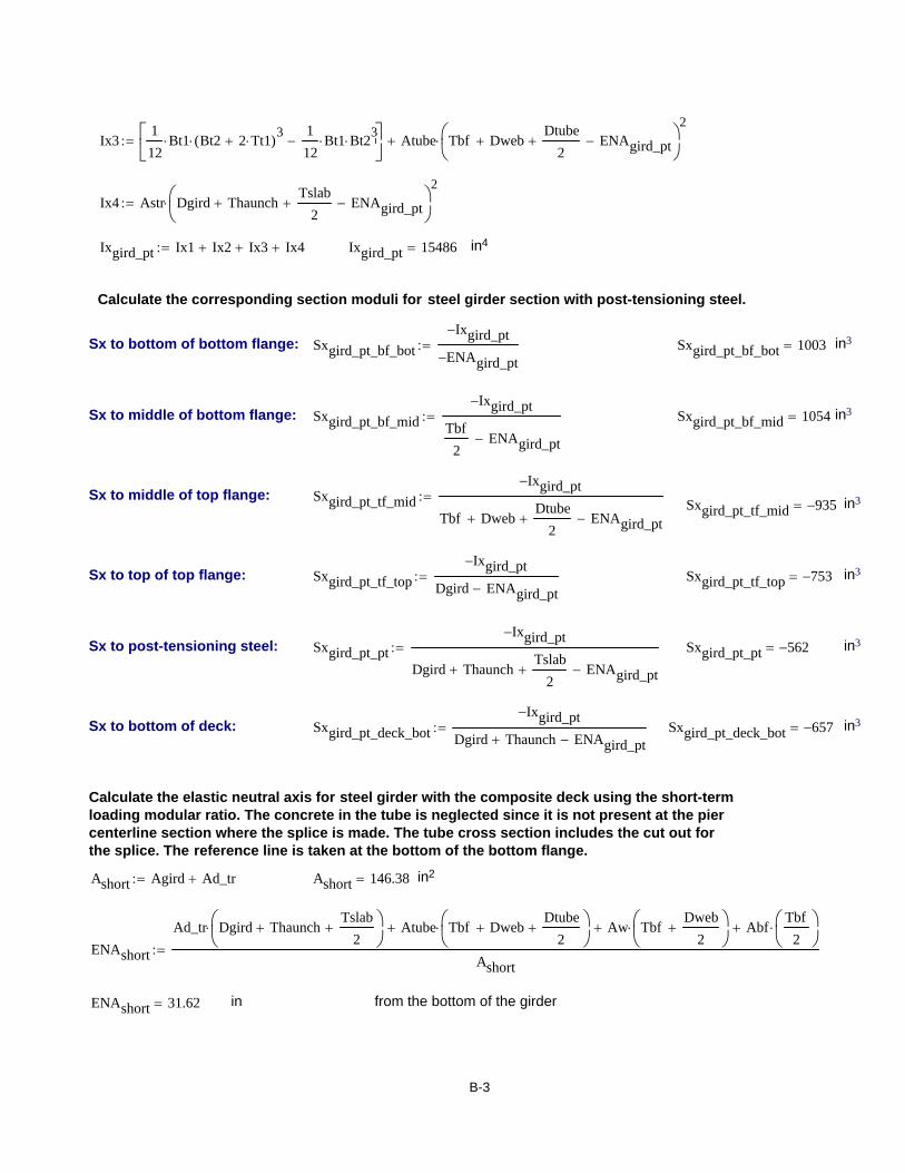
Ix3112
Bt1⋅ Bt2 2 Tt1⋅+( )3⋅
112
Bt1⋅ Bt23⋅−⎡⎢
⎣⎤⎥⎦
Atube Tbf Dweb+Dtube
2+ ENAgird_pt−⎛⎜
⎝⎞⎟⎠
2⋅+:=
Ix4 Astr Dgird Thaunch+Tslab
2+ ENAgird_pt−⎛⎜
⎝⎞⎟⎠
2⋅:=
Ixgird_pt Ix1 Ix2+ Ix3+ Ix4+:= Ixgird_pt 15486= in4
Calculate the corresponding section moduli for steel girder section with post-tensioning steel.
Sx to bottom of bottom flange: Sxgird_pt_bf_botIxgird_pt−
ENAgird_pt−:= Sxgird_pt_bf_bot 1003= in3
Sx to middle of bottom flange: Sxgird_pt_bf_midIxgird_pt−
Tbf2
ENAgird_pt−
:= Sxgird_pt_bf_mid 1054= in3
Sx to middle of top flange: Sxgird_pt_tf_midIxgird_pt−
Tbf Dweb+Dtube
2+ ENAgird_pt−
:= Sxgird_pt_tf_mid 935−= in3
Sx to top of top flange: Sxgird_pt_tf_topIxgird_pt−
Dgird ENAgird_pt−:= Sxgird_pt_tf_top 753−= in3
Sx to post-tensioning steel: Sxgird_pt_ptIxgird_pt−
Dgird Thaunch+Tslab
2+ ENAgird_pt−
:= Sxgird_pt_pt 562−= in3
Sx to bottom of deck: Sxgird_pt_deck_botIxgird_pt−
Dgird Thaunch+ ENAgird_pt−:= Sxgird_pt_deck_bot 657−= in3
Calculate the elastic neutral axis for steel girder with the composite deck using the short-termloading modular ratio. The concrete in the tube is neglected since it is not present at the piercenterline section where the splice is made. The tube cross section includes the cut out forthe splice. The reference line is taken at the bottom of the bottom flange.
Ashort Agird Ad_tr+:= Ashort 146.38= in2
ENAshort
Ad_tr Dgird Thaunch+Tslab
2+⎛⎜
⎝⎞⎟⎠
⋅ Atube Tbf Dweb+Dtube
2+⎛⎜
⎝⎞⎟⎠
⋅+ Aw TbfDweb
2+⎛⎜
⎝⎞⎟⎠
⋅+ AbfTbf
2⎛⎜⎝
⎞⎟⎠
⋅+
Ashort:=
ENAshort 31.62= in from the bottom of the girder
B-3

Calculate the corresponding moment of inertia for steel girder with short-term composite deck.
Ix1112
Bbf⋅ Tbf 3⋅ Abf
Tbf2
ENAshort−⎛⎜⎝
⎞⎟⎠
2⋅+:=
Ix2112
Tweb⋅ Dweb3⋅ Aw Tbf
Dweb2
+ ENAshort−⎛⎜⎝
⎞⎟⎠
2⋅+:=
Ix3112
Bt1⋅ Bt2 2 Tt1⋅+( )3⋅
112
Bt1⋅ Bt23⋅−⎡⎢
⎣⎤⎥⎦
Atube Tbf Dweb+Dtube
2+ ENAshort−⎛⎜
⎝⎞⎟⎠
2⋅+:=
Ix4112
Beffns
⎛⎜⎝
⎞⎟⎠
Tslab3⋅ Ad_tr Dgird Thaunch+
Tslab2
+ ENAshort−⎛⎜⎝
⎞⎟⎠
2⋅+:=
Ixshort Ix1 Ix2+ Ix3+ Ix4+:= Ixshort 42893= in4
Calculate the corresponding section moduli for steel girder with short-term composite deck.
Sx to bottom of bottom flange: Sxshort_bf_botIxshort−
ENAshort−:= Sxshort_bf_bot 1356= in3
Sx to middle of bottom flange: Sxshort_bf_midIxshort−
Tbf2
ENAshort−
:= Sxshort_bf_mid 1389= in3
Sx to middle of top flange: Sxshort_tf_midIxshort−
Tbf Dweb+Dtube
2+ ENAshort−
:=
Sxshort_tf_mid 113328−= in3
Sx to top of top flange: Sxshort_tf_topIxshort−
Tbf Dweb+ Dtube+ ENAshort−:=
Sxshort_tf_top 9796−= in3
Sx to top of deck: Sxshort_deck_topIxshort−
Tbf Dweb+ Dtube+ Thaunch+ Tslab+ ENAshort−:=
Sxshort_deck_top 2789−= in3
B-4
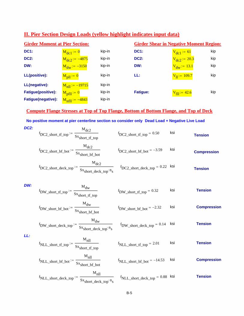
II. Pier Section Design Loads (yellow highlight indicates input data)
Girder Moment at Pier Section: Girder Shear in Negative Moment Region:DC1: Mdc1 0:= kip-in DC1: Vdc1 61:= kip
DC2: Mdc2 4875−:= kip-in DC2: Vdc2 20.3:= kip
DW: Mdw 3150−:= kip-in DW: Vdw 13.1:= kip
LL(positive): Mpll 0:= kip-in LL: Vll 109.7:= kip
LL(negative): Mnll 19715−:= kip-in
Fatigue(positive): Mpfll 0:= kip-in Fatigue: Vfll 42.6:= kip
Fatigue(negative): Mnfll 4843−:= kip-in
Compute Flange Stresses at Top of Top Flange, Bottom of Bottom Flange, and Top of Deck
No positive moment at pier centerline section so consider only Dead Load + Negative Live Load
DC2:fDC2_short_tf_top
Mdc2Sxshort_tf_top
:= fDC2_short_tf_top 0.50= ksi Tension
fDC2_short_bf_botMdc2
Sxshort_bf_bot:= fDC2_short_bf_bot 3.59−= ksi Compression
fDC2_short_deck_topMdc2
Sxshort_deck_top ns⋅:= fDC2_short_deck_top 0.22= ksi Tension
DW:fDW_short_tf_top
MdwSxshort_tf_top
:= fDW_short_tf_top 0.32= ksi Tension
fDW_short_bf_botMdw
Sxshort_bf_bot:= fDW_short_bf_bot 2.32−= ksi Compression
fDW_short_deck_topMdw
Sxshort_deck_top ns⋅:= fDW_short_deck_top 0.14= ksi Tension
LL:
fNLL_short_tf_topMnll
Sxshort_tf_top:= fNLL_short_tf_top 2.01= ksi Tension
fNLL_short_bf_botMnll
Sxshort_bf_bot:= fNLL_short_bf_bot 14.53−= ksi Compression
fNLL_short_deck_topMnll
Sxshort_deck_top ns⋅:= fNLL_short_deck_top 0.88= ksi Tension
B-5

Fatigue:fNFLL_short_tf_top
MnfllSxshort_tf_top
:= fNFLL_short_tf_top 0.49= ksi Tension
fNFLL_short_bf_botMnfll
Sxshort_bf_bot:= fNFLL_short_bf_bot 3.57−= ksi Compression
Compute Force Effects for Strength I, Service II. and Fatigue Limit State Load Combinations
Strength I Limit State: Dead Load + Negative Live Load Effect
MNLL_st 1.25 Mdc2⋅ 1.5 Mdw⋅+ 1.75 Mnll⋅+( ):= MNLL_st 45320−= kip-in Negative
Vst 1.25 Vdc1 Vdc2+( )⋅ 1.5 Vdw⋅+ 1.75 Vll⋅+⎡⎣ ⎤⎦:= Vst 313.25= kip
Service II Limit State: Dead Load + Negative Live Load
MNLL_sv 1.0 Mdc2⋅ 1.0 Mdw⋅+ 1.3 Mnll⋅+( ):= MNLL_sv 33655−= kip-in Negative
ftf_top_sv 1.0 fDC2_short_tf_top⋅ 1.0 fDW_short_tf_top⋅+ 1.3 fNLL_short_tf_top⋅+( ):=
ftf_top_sv 3.44= ksi Tension
fbf_bot_sv 1.0 fDC2_short_bf_bot⋅ 1.0 fDW_short_bf_bot⋅+ 1.3 fNLL_short_bf_bot⋅+( ):=
fbf_bot_sv 24.81−= ksi Compression
fdeck_top_sv 1.0 fDC2_short_deck_top⋅ 1.0 fDW_short_deck_top⋅+ 1.3 fNLL_short_deck_top⋅+( ):=
fdeck_top_sv 1.51= ksi Tension
Fatigue Limit State: Negative Live Load
ftf_top_fat 0.75 fNFLL_short_tf_top⋅( ):= ftf_top_fat 0.37= ksi Tension
fbf_bot_fat 0.75 fNFLL_short_bf_bot⋅( ):= fbf_bot_fat 2.68−= ksi Compression
Vfat Vdc1 Vdc2+ Vdw+ 2 0.75 Vfll⋅( )+:= Vfat 158.30= kip
B-6

III. Pier Section Design ChecksThe concrete in the tube is neglected since it is not present at the pier centerline sectionwhere the splice is made. The tube cross section includes the cut out for the splice.
Strength I Limit State: Negative Flexure (First determine the sequence of events under flexure)
Plastic moment capacity of section without concrete assuming the plastic neutral axis is in web. The referenceaxis is the bottom of the bottom flange.
Comp x( ) Abf− Fy⋅ x Tweb⋅ Fy⋅−:=
Tens x( ) Astr Fy_str⋅ Atube Fy⋅+ Dweb x−( ) Tweb⋅ Fy⋅+:= Func x( ) Tens x( ) Comp x( )+:=
x 1:= Dcp root Func x( ) x, ( ):=Dcp 31.58= in
PNA Dcp Tbf+:=PNA 33.08= in PNA is not in web Dtp Dweb Dcp−:=Dtp 5.08−= in
M1 Fy_str Astr⋅ Dgird Thaunch+Tslab
2+⎛⎜
⎝⎞⎟⎠
⋅:= strands M1 68023= kip-in
M2 Fy Atube⋅ Tbf Dweb+Dtube
2⎛⎜⎝
⎞⎟⎠
+⎡⎢⎣
⎤⎥⎦
⋅:= tube M2 21900= kip-in
web intensionM3 Fy Tweb Dtp( )⋅[ ]
Dtp2
PNA+⎛⎜⎝
⎞⎟⎠
⋅⎡⎢⎣
⎤⎥⎦
⋅:= M3 3875−= kip-in
web incompressionM4 Fy− Tweb Dcp( )⋅[ ]⋅
Dcp2
Tbf+⎛⎜⎝
⎞⎟⎠
⋅:= M4 13647−= kip-in
bottomflangeM5 Fy− Abf⋅
Tbf2
⎛⎜⎝
⎞⎟⎠
⋅:= M5 1013−= kip-in
Mp_web M1 M2+ M3+ M4+ M5+:= Mp_web 71388= kip-in
Plastic moment capacity of section without concrete assuming the plastic neutral axis is in middle of tubebottom wall. Because of cut-out, treat area of tube as concentrated at top wall and bottom wall. The referenceaxis is the bottom of the bottom flange.
Comp2 Abf− Fy⋅ Dweb Tweb⋅ Fy⋅−Atube
4Fy⋅−:= Comp2 2184−= kip
OKTens2 Astr Fy_str⋅
3Atube4
⎛⎜⎝
⎞⎟⎠
Fy⋅+:= Tens2 2095= kip
Dcp Dweb:=Dcp 26.50= inPNA Dcp Tbf+:=PNA 28.00= inDtp Dweb Dcp−:=Dtp 0.00= in
M1 Fy_str Astr⋅ Dgird Thaunch+Tslab
2+⎛⎜
⎝⎞⎟⎠
⋅:= strands M1 68023= kip-in
M2 FyAtube
2⎛⎜⎝
⎞⎟⎠
⋅ Tbf Dweb+ Dtube+( )⋅:= top wallof tube
M2 12319= kip-in
B-7

bottom wallof tubeM3 0:= M3 0= kip-in
webM4 Fy− Tweb Dweb( )⋅[ ]⋅
Dweb2
Tbf+⎛⎜⎝
⎞⎟⎠
⋅:= M4 9772−= kip-in
bottomflangeM5 Fy− Abf⋅
Tbf2
⎛⎜⎝
⎞⎟⎠
⋅:= M5 1013−= kip-in
Mp_tube M1 M2+ M3+ M4+ M5+( )−:= Mp_tube 69557−= kip-in
Determine conditions when deck decompresses at top surface. Use transformed section basedon short-term loading concrete in deck. Prestress in deck is based on an estimate of 15% timedependent prestress losses and an initial prestress of 70% of Fu of strands.
0.7 Fu_str⋅ 189= ksi
Moment when deck decompresses at top surface .
f_str_losses 0.7 Fu_str⋅ 1 0.15−( )⋅:= f_str_losses 161= ksi
bridge_deck_width W:= bridge_deck_width 376.50= in
fdeck_prestress4 Astr⋅ f_str_losses⋅
Tslab bridge_deck_width( )⋅:= fdeck_prestress 1.389= ksi
Mdeck_top_decomp ns Sxshort_deck_top⋅ fdeck_prestress⋅:= Mdeck_top_decomp 30990−= kip-in
Stresses when deck decompresses at top surface.
fdeck_top_decomp_bf_botMdeck_top_decomp
Sxshort_bf_bot
⎛⎜⎝
⎞⎟⎠
:= fdeck_top_decomp_bf_bot 22.85−=
fdeck_top_decomp_tf_topMdeck_top_decomp
Sxshort_tf_top
⎛⎜⎝
⎞⎟⎠
:= fdeck_top_decomp_tf_top 3.16=
Determine conditions when deck fully decompresses. These conditions control the stressesthat develop on the section without the deck (the steel girder and post-tensioning strands),under moments that exceed the moment causing deck decompression.
Moment when deck fully decompresses.
M1full_decomp f_str_losses− Astr⋅ Dgird Thaunch+Tslab
2+ ENAgird_pt−⎛⎜
⎝⎞⎟⎠
⋅:= M1full_decomp 28818−= kip-in
M2full_decomp fdeck_prestress ns⋅ Sxgird_pt_deck_bot⋅:= M2full_decomp 7305−= kip-in
Mfull_decomp M1full_decomp M2full_decomp+:= Mfull_decomp 36123−= kip-in
B-8

Stresses when deck fully decompresses.
ffull_decomp_bf_botf_str_losses− Astr⋅
Agird
M2full_decompSxgird_pt_bf_bot
⎛⎜⎝
⎞⎟⎠
+:= ffull_decomp_bf_bot 26.68−= ksi
ffull_decomp_bf_midf_str_losses− Astr⋅
Agird
M2full_decompSxgird_pt_bf_mid
⎛⎜⎝
⎞⎟⎠
+:= ffull_decomp_bf_mid 26.32−= ksi
ffull_decomp_tf_topf_str_losses− Astr⋅
Agird
M2full_decompSxgird_pt_tf_top
⎛⎜⎝
⎞⎟⎠
+:= ffull_decomp_tf_top 9.69−= ksi
ffull_decomp_tf_midf_str_losses− Astr⋅
Agird
M2full_decompSxgird_pt_tf_mid
⎛⎜⎝
⎞⎟⎠
+:= ffull_decomp_tf_mid 11.58−= ksi
ffull_decomp_pt f_str_lossesM2full_decomp
Sxgird_pt_pt
⎛⎜⎝
⎞⎟⎠
+:= ffull_decomp_pt 173.65= ksi
Determine moments which cause yielding. Determine the additional moment needed to causeyield (using section without concrete) and add to moment at time deck fully decompressed
Myield_bf Sxgird_pt_bf_bot Fy− ffull_decomp_bf_bot−( )⋅ Mfull_decomp+:= Myield_bf 59509−= kip-in
Myield_tf Sxgird_pt_tf_top Fy ffull_decomp_tf_top−( )⋅ Mfull_decomp+:= Myield_tf 81096−= kip-in
Myield_pt Sxgird_pt_pt Fy_str ffull_decomp_pt−( )⋅ Mfull_decomp+:= Myield_pt 75099−= kip-in
Strength I Limit State: Negative Flexure (sequence of events)
Deck decompresses at top surface (joint would open if at pier centerline)•
Bottom flange yields•
Section reaches plastic moment•
Post-tensioning steel yields based on elastic section (inaccurate)•
Top flange yields based on elastic section (inaccurate) •
Factored design Strength I design moment•
Mdeck_top_decomp 30990−= kip-in
Myield_bf 59509−= kip-in
Mp_tube 69557−= kip-in
Myield_pt 75099−= kip-in
Myield_tf 81096−= kip-in
MNLL_st 45320−= kip-in
B-9

Strength I Limit State: Negative Flexure (section capacity using Appendix A of AASHTO)
Dc ENAgird_pt Tbf−:= Dc 13.95= inλw 2
DcTweb
:= λrw 5.729000
Fy:=
Dcp 26.50= in
λw 55.78= < λrw 137.27= OK, Appendix A can be used
Consider the web slenderness and calculate the web plastification factors
Mp Mp_tube:= Mp 69557= kip-in
Myt Myield_tf:= Myt 81096= kip-in
Myc Myield_bf:= Myc 59509= kip-inMy min Myt Myc, ( ):= My 59509= kip-in
λpw1
29000Fy
0.54MpMy
0.09−
:= λpw1 44.50= λpw2 λrwDcDcp
⎛⎜⎝
⎞⎟⎠
⋅:= λpw2 72.24=
λpw min λpw1 λpw2, ( ):=
2DcpTweb
106.00= > λpw 44.50= Not compact section
λw 55.78= < λrw 137.27= Noncompact web section
λpw3 λpwDcDcp
⎛⎜⎝
⎞⎟⎠
⋅:= λpw3 23.42=
Rpc 1 1MycMp
−⎛⎜⎝
⎞⎟⎠
λw λpw3−
λrw λpw3−−⎡⎢
⎣⎤⎥⎦
MpMyc
:= Rpc 1.12= < MpMyc
1.17= OK
Rpt 1 1MytMp
−⎛⎜⎝
⎞⎟⎠
λw λpw3−
λrw λpw3−−⎡⎢
⎣⎤⎥⎦
MpMyt
:= Rpt 0.90= < MpMyt
0.86= NG
RptMpMyt
:=Nominal resistance for tension flange yielding
Mnt Rpt Myt⋅:= Mnt 69557= kip-in
Consider the compression flange slenderness
λfBbf
2 Tbf⋅:= λpf 0.38
29000Fy
⋅:=
λf 6.00= < λpf 9.15= Compact flange
Mnc_cf Rpc Myc⋅:= Mnc_cf 66701= kip-in
B-10

Consider lateral-torsional buckling
rtBbf
12 113
⎛⎜⎝
⎞⎟⎠
Dc Tweb⋅
Bbf Tbf⋅⋅+⎡⎢
⎣⎤⎥⎦
:= rt 4.99=
KTDweb Tweb3
⋅
3Bbf Tbf 3
⋅
3+
2 Tt2⋅ Tt1⋅ Bt1 Tt2−( )2⋅ Bt2 Tt1+( )2
⋅
Bt1 Tt2−( ) Tt2⋅ Bt2 Tt1+( ) Tt1⋅++:=
J KT:= J 479= in4
Sxc Sxgird_pt_bf_bot:= Sxc 1003= in3
Sxt Sxgird_pt_tf_top:= Sxt 753= in3
h DwebDtube
2+
Tbf2
+:= h 31.25= in
Fyr1 0.7Fy:= Fyr2 FySxtSxc
⎛⎜⎝
⎞⎟⎠
⋅:=
Fyr min Fyr1 Fyr2, ( ):= Fyr 35.00= ksi
Lp rt29000
Fy⋅:= Lp 120= in
Lr 1.95 rt⋅29000
Fyr⎛⎜⎝
⎞⎟⎠
⋅J
Sxc h⋅1 1 6.76
Fyr29000
Sxc h⋅J
⋅⎛⎜⎝
⎞⎟⎠
2⋅++⋅:= Lr 1416= in
Lb100 12⋅
2:= Span is 100 ft. Single cross-frame at midspan Lb 600= in
Cb calculation:M0 will be midspan moment
Mdc1_pos_midspan 17500:= Mdc2_pos_midspan 2700:= Mdw_pos_midspan 1700:= Mll_neg_midspan 7200−:=
Mmidspan_min 1.25 Mdc1_pos_midspan Mdc2_pos_midspan+( )⋅ 1.5 Mdw_pos_midspan⋅+ 1.75 Mll_neg_midspan⋅+⎡⎣ ⎤⎦:=
Mmidspan_min 15200= kip-in
M0 Mmidspan_min−:= M0 15200−=
Mmid will be moment halfway between pier and midspan
Mdc1_pos_q 13000:= Mdc2_pos_q 0:= Mdw_pos_q 0:= Mll_neg_q 11000−:=
Mq_min 1.25 Mdc1_pos_q Mdc2_pos_q+( )⋅ 1.5 Mdw_pos_q⋅+ 1.75 Mll_neg_q⋅+⎡⎣ ⎤⎦:=
Mq_min 3000−= kip-in
Mmid Mq_min−:= Mmid 3000=
B-11

Determine M1 and M2 (moment at pier)
M1 2 Mmid⋅ M2−:= M1 6319−= > M0 15200−= OK
M2 MNLL_st−:= M2 45320= kip-in
Determine Cb from M1 and M2
Cb 1.75 1.05M1M2
⎛⎜⎝
⎞⎟⎠
⋅− 0.3M1M2
⎛⎜⎝
⎞⎟⎠
2⋅+:= Cb 1.90=
Since Lp<Lb<Lr
Mnc1 Cb 1 1Fyr Sxc⋅
Rpc Myc⋅−⎛⎜
⎝⎞⎟⎠
Lb Lp−
Lr Lp−⎛⎜⎝
⎞⎟⎠
−⎡⎢⎣
⎤⎥⎦
⋅ Rpc⋅ Myc⋅:= Mnc1 104620= kip-in
Mnc2 Rpc Myc⋅:= Mnc2 66701= kip-in
Mnc_ltb min Mnc1 Mnc2, ( ):= Mnc_ltb 66701= kip-in
Nominal resistance for compression flange
Mnc min Mnc_cf Mnc_ltb, ( ):= Mnc 66701= kip-in
Strength I Limit State: Negative Flexure (section capacity check) Note: The pier section design iscontrolled by splice. Thesecalculations only show adequacyof cross section away from splice.
Mu MNLL_st:= ϕf 1.0:=
Mu 45320= kip-in
Mu 45320= < ϕf Mnc⋅ 66701= O.K.
< ϕf Mnt⋅ 69557= O.K.
Strength I Limit State: Shear
Nominal shear resistance. Transverse stiffener spacing is 1/4 of span. Design as unstiffened web with k=5):
Vp 0.58 Fy⋅ Dweb⋅ Tweb⋅:=
Av1DwebTweb
:= Bv1 1.1229000 5⋅
Fy⋅:= Cv1 1.40
29000 5⋅Fy
⋅:=
Av1 53.00= Bv1 60.31= Cv1 75.39=
C 1.0 Av1 Bv1<if
1.10Av1
29000 5⋅Fy
⋅ Bv1 Av1≤ Cv1≤if
1.52
Av12
29000 5⋅Fy
⋅ Av1 Cv1>if
:= : plastic
: inelastic
: elastic
C 1.00=
B-12

Vn C Vp⋅:= Vn 384.25= kip Vr 1 Vn⋅:= Vr 384.25= kip
Vst 313.25= < Vr 384.25= O.K.
Service II Limit State: Negative Flexure (composite section with Rh=1)
ftf_top_sv 3.44= ksi Top flange (Tension)
fbf_bot_sv 24.81−= ksi Bottom Flange (Compression)
fallowable 0.95 Fy⋅:= fallowable 47.50= ksi
ftf_top_sv 3.44= < fallowable 47.50= O.K.
fbf_bot_sv 24.81= < fallowable 47.50= O.K.
Service II Limit State: Check Compressive Stress Against Web Bend Buckling
Dc ENAshort Tbf−:= Dc 30.12= kw9
DcDweb
⎛⎜⎝
⎞⎟⎠
2:= kw 6.97=
Fcrw 0.9( ) 29000⋅kw
DwebTweb
⎛⎜⎝
⎞⎟⎠
2⋅:= Fcrw 64.72= ksi
fbf_bot_sv 24.81= < Fcrw 64.72= O.K.
Service II Limit State: Check Moment at Post-Tensioned Deck Joint Opening
As determined above:
Moment at which deck decompresses at top surface (joint would open if•at pier centerline).
Service II Limit State Moment at pier section•
Service II Limit State Moment at pier section exceeds the moment at•which the deck decompresses at the top surface by 10%. This is only aproblem if the deck joint is located directly at the pier section. If the centerdeck panel is centered on the pier section, the tensile stress of theconcrete can be utilized, and the nearest joints may not open.
Note that these calculations are based on the exterior girder Beff. A•similar check was performed for the interior girder, and the deck doesnot decompress at the top surface under the Service II Limit StateMoment at the pier, because the wider Beff of the interior girderincreases the section modulus.
Mdeck_top_decomp 30990−= kip-in
MNLL_sv 33655−= kip-in
B-13

Fatigue Limit State: Negative Flexure
ftf_top_fat 0.37= ksi Tension
fbf_bot_fat 2.68−= ksi Compression - Do Not Consider
Nominal fatigue resistance at bearing stiffener near pier section:
Condition 1: Condition 2:
n 1.5:= ADTT_SL 3000:=
N 365 75⋅ n⋅ ADTT_SL⋅:= N 1.23 108×=
A_bs 44 108⋅:= For Fatigue Category C' : ΔF_TH_bs 12:=
ΔFn_bs1A_bs
N⎛⎜⎝
⎞⎟⎠
1
3:= ΔFn_bs1 3.29= ΔFn_bs2
12
ΔF_TH_bs⋅:= ΔFn_bs2 6.00=
ΔFn_bs ΔFn_bs1 ΔFn_bs1 ΔFn_bs2≥if
ΔFn_bs2 otherwise
:= ΔFn_bs 6.00=
ftf_top_fat 0.37= < ΔFn_bs 6.00= O.K.
Nominal fatigue resistance at shear stud near pier section:
Condition 1: Condition 2:
ΔF_TH_s 10:=A_s 44 108⋅:= For Fatigue Category C :
ΔFn_s1A_sN
⎛⎜⎝
⎞⎟⎠
1
3:= ΔFn_s1 3.29= ΔFn_s2
12
ΔF_TH_s⋅:= ΔFn_s2 5.00=
ΔFn_s ΔFn_s1 ΔFn_s1 ΔFn_s2≥if
ΔFn_s2 otherwise
:= ΔFn_s 5.00=
ftf_top_fat 0.37= < ΔFn_s 5.00= O.K.
Fatigue Limit State: Shear
Vfat 158.30= kip
Note: The web was designed for the Strength I limit state as unstiffened. Calculations for the Strength Ilimit state show that the web shear capacity (Vn = Vcr) equals Vp (i.e., C = 1.0) even though the web istreated as unstiffened (AASHTO LRFD Article 6.10.9.2). As shown, the shear capacity exceeds the sheardemand for the Strength I load combination (Vst) and therefore the requirement of AASHTO LRFD Article6.10.5.3 (Vu = Vfat < Vcr) is also satisfied. (Strictly speaking, since the web is treated as unstiffened, andalso because this is an end panel AASHTO LRFD Article 6.10.3.3 does not apply).
B-14

Part 2. Bolted Field Splice Preliminary Design at Pier Section
I. Cross Section Information (yellow highlight indicates input data)
Yield strength: Fy 50= ksi
16x8x0.375
26.5x0.5
18x1.5(unit: in)
Tensile strength: Fu 65:= ksi
Tube horizontal plate thickness: Tt1 0.38= inNote that tube has 5 in.cut out on each sidewall for splice access.Tube vertical plate thickness: Tt2 0.38= in
Tube horizontal plate width: Bt1 16.00= in
Tube vertical plate width: Bt2 7.25= in
Bottom flange thickness: Tbf 1.50= in
Bottom flange width: Bbf 18.00= in
Web thickness: Tweb 0.50= in
Post-tensioning in Deck (per girder)Web depth: Bweb Dweb:= Dweb 26.50= in
Number of Strands: Nstr 30=Bolt diameter: dbolt 0.875:= in
Area of Strands: Astr 6.51= in2Bolt std. hole width: dhole 1.0:= in
Bolt tensile strength: Fubolt 120:= ksi Short-term Modular Ratio: ns 8=
Area of bottom flange Abf 27= in2
Area of tube at cut-out at pier section Atube 13.6875= in2
Area of one bolt Aboltπ
4dbolt2⋅:= Abolt 0.6013= in2
II. Flange Splice Design Loads
Girder Moment at Splice Locations:DC1: Mdc1 0= kip-in
DC2: Mdc2 4875−= kip-in
DW: Mdw 3150−= kip-in
LL(positive): Mpll 0.00= kip-in
LL(negative): Mnll 19715−= kip-in
Fatigue(positive): Mpfll 0= kip-in
Fatigue(negative): Mnfll 4843−= kip-in
B-15

Splices are designed for Strength I, Service II, and Fatigue Limit States.
Section Modulus - at midthickness of the top flange (tube) and bottom flangeFor steel girder plus post-tensioning steel
Stoppt Sxgird_pt_tf_mid:= Stoppt 935−= in3
Sbotpt Sxgird_pt_bf_mid:= Sbotpt 1054= in3
For steel girder with short term concrete deck
Stopshort Sxshort_tf_mid:= Stopshort 113328−= in3
Sbotshort Sxshort_bf_mid:= Sbotshort 1389= in3
Sdeckshort Sxshort_deck_top:= Sdeckshort 2789−= in3
Flange Stress Computation:
Case 1: Dead Load + Positive Live Load (there is no positive moment at pier centerline section)Case 2: Dead Load + Negative Live Load==> Case 2 controls, therefore only check Case 2
DC2: fdeckDC2_shortMdc2
Sdeckshort ns⋅:= fdeckDC2_short 0.22= ksi Tension
ftopDC2_shortMdc2
Stopshort:= ftopDC2_short 0.04= ksi Tension
fbotDC2_shortMdc2
Sbotshort:= fbotDC2_short 3.51−= ksi Compression
fdeckDW_shortMdw
Sdeckshort ns⋅:= fdeckDW_short 0.14= ksi TensionDW:
ftopDW_shortMdw
Stopshort:= ftopDW_short 0.03= ksi Tension
fbotDW_shortMdw
Sbotshort:= fbotDW_short 2.27−= ksi Compression
-LL:fdeckNLL_short
MnllSdeckshort ns⋅
:= fdeckNLL_short 0.88= ksi Tension
ftopNLL_shortMnll
Stopshort:= ftopNLL_short 0.17= ksi Tension
fbotNLL_shortMnll
Sbotshort:= fbotNLL_short 14.19−= ksi Compression
B-16

Strength I Limit State: Dead Load + Negative Live Load
MNLL_st 1.25 Mdc2⋅ 1.5 Mdw⋅+ 1.75 Mnll⋅+( ):= MNLL_st 45320−= kip-in Negative
Flange stresses are stresses when deck fully decompresses plus additionalstresses for remaining moment up the Strength Limit State moment demand.
ftopNLL_st ffull_decomp_tf_midMNLL_st Mfull_decomp−
Stoppt+:= ftopNLL_st 1.75−=
fbotNLL_st ffull_decomp_bf_midMNLL_st Mfull_decomp−
Sbotpt+:= fbotNLL_st 35.05−=
Service II Limit State: Dead Load + Negative Live Load
ftopNLL_sv 1.0 ftopDC2_short⋅ 1.0 ftopDW_short⋅+ 1.3 ftopNLL_short⋅+( ):= ftopNLL_sv 0.30= ksi Tension
fbotNLL_sv 1.0 fbotDC2_short⋅ 1.0 fbotDW_short⋅+ 1.3 fbotNLL_short⋅+( ):= fbotNLL_sv 24.22−= ksi Compression
MNLL_sv 1.0 Mdc2⋅ 1.0 Mdw⋅+ 1.3 Mnll⋅+( ):= MNLL_sv 3.37− 104×= kip-in Negative
fdeckNLL_sv 1.0 fdeckDC2_short⋅ 1.0 fdeckDW_short⋅+ 1.3 fdeckNLL_short⋅+( ):= fdeckNLL_sv 1.508= ksi Compression
Fatigue Limit State: Negative Live Load
ftopNFLL_shortMnfll
Stopshort:= ftopNFLL_short 0.04= ksi Tension
fbotNFLL_shortMnfll
Sbotshort:= fbotNFLL_short 3.49−= ksi Compression
ftopNLL_fa 0.75 ftopNFLL_short⋅:= ftopNLL_fa 0.03= ksi Tension
fbotNLL_fa 0.75 fbotNFLL_short⋅:= fbotNLL_fa 2.61−= ksi Compression
MNLL_fa 0.75 Mnfll⋅:= MNLL_fa 3.63− 103×= kip-in Negative
B-17
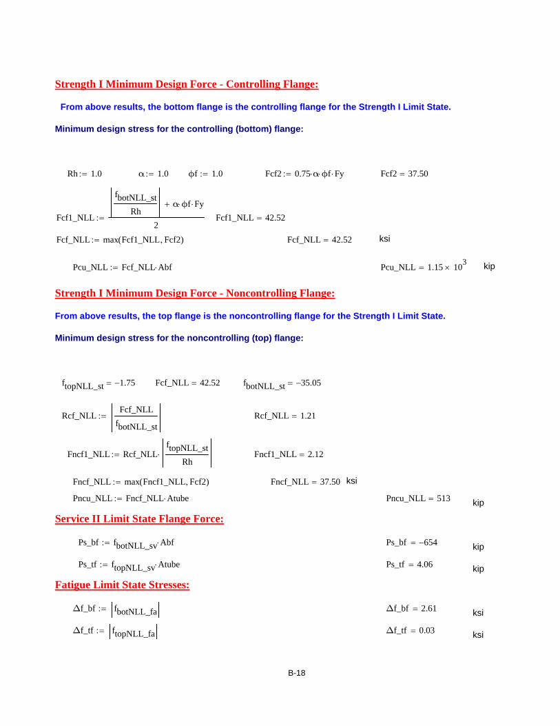
Strength I Minimum Design Force - Controlling Flange:
From above results, the bottom flange is the controlling flange for the Strength I Limit State.
Minimum design stress for the controlling (bottom) flange:
Rh 1.0:= α 1.0:= ϕf 1.0:= Fcf2 0.75 α⋅ ϕf⋅ Fy⋅:= Fcf2 37.50=
Fcf1_NLL
fbotNLL_stRh
α ϕf⋅ Fy⋅+
2:= Fcf1_NLL 42.52=
Fcf_NLL max Fcf1_NLL Fcf2, ( ):= Fcf_NLL 42.52= ksi
Pcu_NLL Fcf_NLL Abf⋅:= Pcu_NLL 1.15 103×= kip
Strength I Minimum Design Force - Noncontrolling Flange:
From above results, the top flange is the noncontrolling flange for the Strength I Limit State.
Minimum design stress for the noncontrolling (top) flange:
ftopNLL_st 1.75−= Fcf_NLL 42.52= fbotNLL_st 35.05−=
Rcf_NLLFcf_NLL
fbotNLL_st:= Rcf_NLL 1.21=
Fncf1_NLL Rcf_NLLftopNLL_st
Rh⋅:= Fncf1_NLL 2.12=
Fncf_NLL max Fncf1_NLL Fcf2, ( ):= Fncf_NLL 37.50= ksi
Pncu_NLL Fncf_NLL Atube⋅:= Pncu_NLL 513= kip
Service II Limit State Flange Force:
Ps_bf fbotNLL_sv Abf⋅:= Ps_bf 654−= kip
Ps_tf ftopNLL_sv Atube⋅:= Ps_tf 4.06= kip
Fatigue Limit State Stresses:
Δf_bf fbotNLL_fa:= Δf_bf 2.61= ksi
Δf_tf ftopNLL_fa:= Δf_tf 0.03= ksi
B-18

III. Design Bottom Flange Splice (yellow highlight indicates input)
Splice Plate Dimensions:
Try 1.5 x 18" outside splice plate (no inside plate)
Thickness of the outside splice palte: Tout 1.5:= in
Width of the outside splice plate: Bout 18:= in
Aout Tout Bout⋅:= Aout 27.00= in2
Yielding and Fracture of Splice Plates:Compression.
Pcu_NLL 1148=
Check compression yielding of outside splice plate:
Prout_yield_comp 0.90 Fy⋅ Tout⋅ Bout⋅:= Prout_yield_comp 1215= kip
Pcu_NLL 1148= < Prout_yield_comp 1215= O.K.
Compression stress on actual net section of outside splice plate.This stress check is not required, but shows that the net sectionis somewhat small when 6 bolts per row are used:
nb 6:=
Pcu_NLL
Aout nb dbolt116
+⎛⎜⎝
⎞⎟⎠
⋅ Tout⋅⎡⎢⎣
⎤⎥⎦
−
61.85= ksi
Yielding of Flange and Fracture of Flange at Holes:
Compression. Note that flange stress and the flange splicedesign stress are both less than yield stress.
fbotNLL_st 35.05−= ksi O.K.
Stress on flange and splice plate are similar. They have thesame width and thickness. Fcf_NLL 42.52= ksi O.K.
Bolts - Shear:
Determine the number of bolts for the bottom flange splice plates that are required to develop the Strength Idesign force in the flange in shear assuming the bolts in the connection have slipped and gone into bearing.
Pcu_NLL 1148=
Assume that the threads are excluded from the shear planes and the design force acts on one shear plane.
Ns1 1:=
Rn_bf 0.48 Abolt⋅ Fubolt⋅ Ns1⋅:= Rn_bf 34.64= kip
Ru_bf 0.80 Rn_bf⋅:= Ru_bf 27.71= kip
Nbf_eachsidePcu_NLL
Ru_bf:= Nbf_eachside 41.44=
The minimum number of bolts required on each side of the splice to resist the Strength I flange design forcein shear is 42. The number of bolts used is 48, 8 rows of 6 bolts.
B-19

Bolts - Slip Resistance:
Bolted flange splice designed as slip-critical connections for the Service II flange design force.
Ps_bf 654−=
Determine the factored resistance per bolt assuming a Class B surface condition.
Minimum required bolt tension: Pt 39:= kip
Hole size factor: Kh 1.0:=
Surface condition factor for Class B surface conditions: Ks 0.5:=
Rn_slip_bf Kh Ks⋅ Ns1⋅ Pt⋅:=
Rr_slip_bf Rn_slip_bf:= Rr_slip_bf 19.50= kip
Nbf_eachside_slip_bfPs_bf
Rr_slip_bf:= Nbf_eachside_slip_bf 33.54=
The minimum number of bolts required on each side of the splice to resist the Service II flange design forceagainst slip is 34. The number of bolts used is 48, 8 rows of 6 bolts.
Bolts - Minimum Spacing:
dbolt 0.875= s_min 3 dbolt⋅:= s_min 2.625= in
Bolts - Edge Distance and Spacing for Splice Plate:
The edge distance is 1.5in. and the bolt spacing is 3*dbolt= 2.625 in.
Bolts - Bearing at Bolt Holes on Splice Plate:
Pcu_NLL 1148=
The clear end distance between the edge of the hole and the end of the splice plate:
Lc1_bf 1.5dhole
2−:= Lc1_bf 1.00= in
The clear distance between edges of adjacent holes in the direction of the force is computed as:
Lc2_bf 3 dbolt⋅ dhole−:= Lc2_bf 1.63= in
For the outside splice plate:
n1: Number of bolts in the end row n1 6:=
n2: Number of remaining bolts n2 48 n1−:=
B-20

Rn1 n1 1.2 Lc1_bf⋅ Tout⋅ Fu⋅( )⋅:= Rn2 n2 1.2 Lc2_bf⋅ Tout⋅ Fu⋅( )⋅:=
Rn_bf_bearing Rn1 Rn2+:= Rn_bf_bearing 8.69 103×= kips
Rr_bf_bearing 0.80 Rn_bf_bearing⋅:= Rr_bf_bearing 6.95 103×= kips
Pcu_NLL 1148= < Rr_bf_bearing 6950= O.K.
Bolts - Bearing at Bolt Holes on Flange:
Note flange is same thickness as splice plate and edge distance is greater - no check required.
Fatigue of Flange at Bolt Holes:
Load-induced fatigue:
Δf_bf 2.61= ksi
Nominal fatigue resistance:
Condition 1: Condition 2:
n 1.5:= ADTT_SL 3000:= ΔF_TH 16:=
N 365 75⋅ n⋅ ADTT_SL⋅:= N 1.23 108×=
A 120 108⋅:= For Fatigue Category B:
ΔFn1AN
⎛⎜⎝
⎞⎟⎠
1
3:= ΔFn1 4.60= ΔFn2
12
ΔF_TH⋅:= ΔFn2 8.00=
ΔFn ΔFn1 ΔFn1 ΔFn2≥if
ΔFn2 otherwise
:= ΔFn 8.00=
Δf_bf 2.61= < ΔFn 8.00= O.K.
Fatigue of Splice Plate at Bolt Holes:
Load-induced fatigue:
Δf_out Δf_bfAbfAout
⋅:= Δf_out 2.61= ksi < ΔFn 8.00= O.K.
B-21

IV. Design Top Flange Splice (yellow highlight indicates input)Splice plates are on top wall and bottom wall of tube.•The top wall top splice plate, the top wall bottom splice plate, and the bottom wall top splice plate•are identical. Call this plate the outside plate.The bottom wall bottom splice plate pair (adjacent to web) differ. Call these plates the inside plate.•
Splice Plate Dimensions:Try 0.5 x 13.5" plate for outside splice plate
Thickness of the outside splice plate: Tout_tf 0.5:= in
Width of the outside splice plate: Bout_tf 13.5:= in
Try (2) 0.5 x 6.0" plates for inside splice plate
Thickness of the inside top wall splice plate: Tin_tf 0.5:= in
Width of the inside top wall splice plate: Bin_tf 2 6⋅:= in
Aout_tf Tout_tf Bout_tf⋅:= Aout_tf 6.75= in2
Ain_tf Tin_tf Bin_tf⋅:= Ain_tf 6.00= in2
n1_tf: Number of bolts across the width of single splice plate n1_tf 4:=
Check 1Ain_tfAout_tf
−⎛⎜⎝
⎞⎟⎠
100⋅ 11.11= The areas are essentially within ten percent ==> O.K.
Yielding and Fracture of Splice Plates:Total Tension (apply 1/2 to set of plates on each tube wall and apply 1/2 of that to each plate):
Pncu_NLL 513=
For yielding on the outside splice plate :
Prout_yield_ten 0.95 Fy⋅ Tout_tf⋅ Bout_tf⋅:= Prout_yield_ten 320.63= kip
Pncu_NLL2 2⋅
128= < Prout_yield_ten 321= O.K.
For yielding on the inside splice plates :
Prin_yielding_ten 0.95 Fy⋅ Tin_tf⋅ Bin_tf⋅:= Prin_yielding_ten 285.00= kip
Pncu_NLL2 2⋅
128= < Prin_yielding_ten 285= O.K.
For fracture of the outside splice plate:→
Bn_out_tf Bout_tf n1_tf dhole⋅−:= Bn_out_tf 9.50= in
An_out_tf Bn_out_tf Tout_tf⋅:= An_out_tf 4.75= in2
Prout_fra_tf 0.8 Fu⋅ An_out_tf⋅:= Prout_fra_tf 247.00= kip
Pncu_NLL2 2⋅
128= < Prout_fra_tf 247= O.K.
B-22
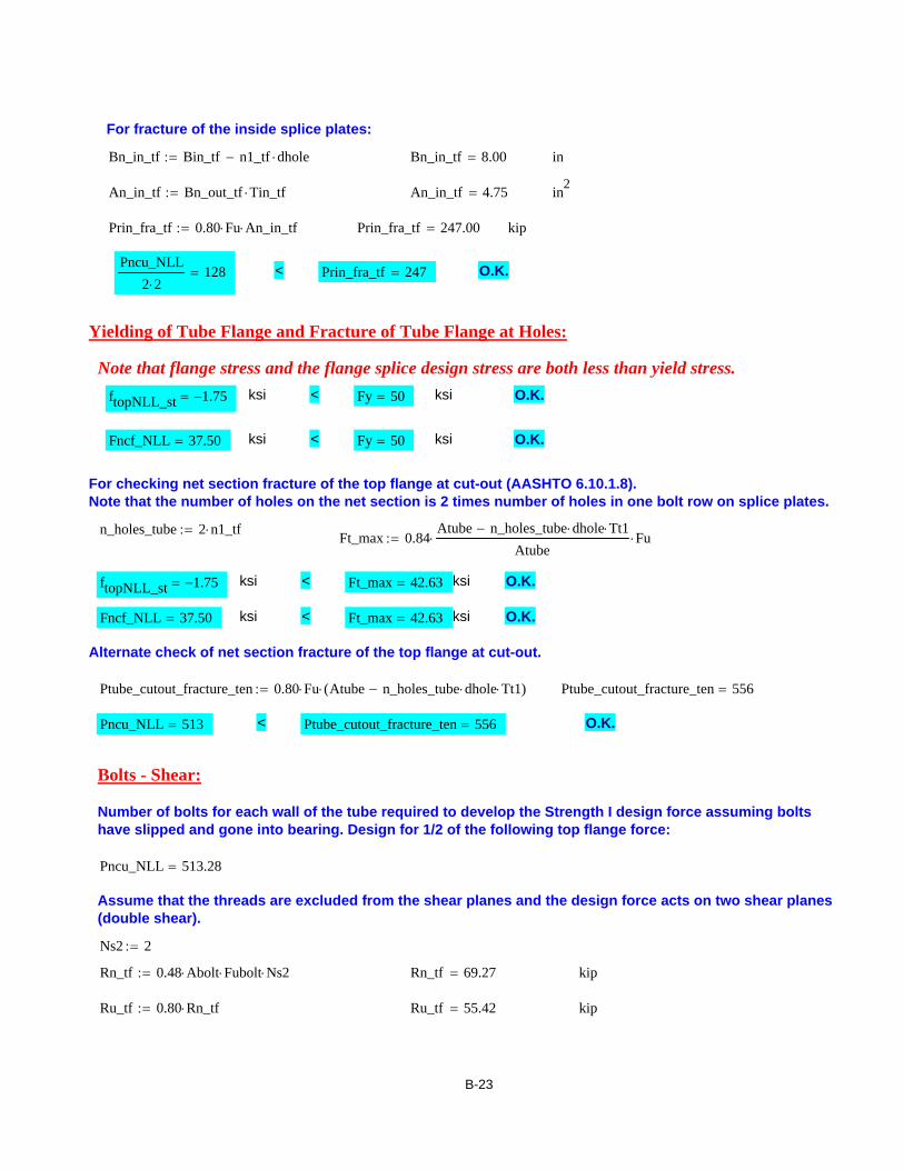
For fracture of the inside splice plates:
Bn_in_tf Bin_tf n1_tf dhole⋅−:= Bn_in_tf 8.00= in
An_in_tf Bn_out_tf Tin_tf⋅:= An_in_tf 4.75= in2
Prin_fra_tf 0.80 Fu⋅ An_in_tf⋅:= Prin_fra_tf 247.00= kip
Pncu_NLL2 2⋅
128= < Prin_fra_tf 247= O.K.
Yielding of Tube Flange and Fracture of Tube Flange at Holes:
Note that flange stress and the flange splice design stress are both less than yield stress.ftopNLL_st 1.75−= ksi < Fy 50= ksi O.K.
Fncf_NLL 37.50= ksi < Fy 50= ksi O.K.
For checking net section fracture of the top flange at cut-out (AASHTO 6.10.1.8).Note that the number of holes on the net section is 2 times number of holes in one bolt row on splice plates.
n_holes_tube 2 n1_tf⋅:= Ft_max 0.84Atube n_holes_tube dhole⋅ Tt1⋅−
Atube⋅ Fu⋅:=
ftopNLL_st 1.75−= ksi < Ft_max 42.63= ksi O.K.
Fncf_NLL 37.50= ksi < Ft_max 42.63= ksi O.K.
Alternate check of net section fracture of the top flange at cut-out.
Ptube_cutout_fracture_ten 0.80 Fu⋅ Atube n_holes_tube dhole⋅ Tt1⋅−( )⋅:= Ptube_cutout_fracture_ten 556=
Pncu_NLL 513= < Ptube_cutout_fracture_ten 556= O.K.
Bolts - Shear:
Number of bolts for each wall of the tube required to develop the Strength I design force assuming boltshave slipped and gone into bearing. Design for 1/2 of the following top flange force:
Pncu_NLL 513.28=
Assume that the threads are excluded from the shear planes and the design force acts on two shear planes(double shear).
Ns2 2:=
Rn_tf 0.48 Abolt⋅ Fubolt⋅ Ns2⋅:= Rn_tf 69.27= kip
Ru_tf 0.80 Rn_tf⋅:= Ru_tf 55.42= kip
B-23
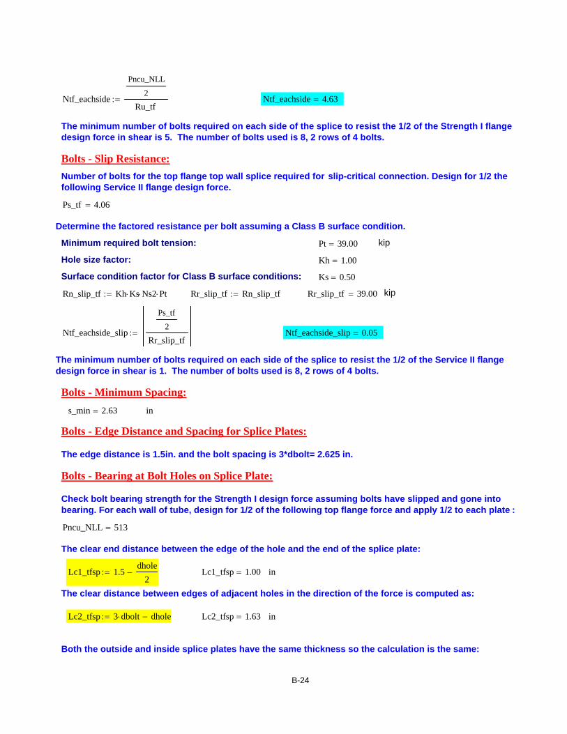
Ntf_eachside
Pncu_NLL
2
Ru_tf:= Ntf_eachside 4.63=
The minimum number of bolts required on each side of the splice to resist the 1/2 of the Strength I flangedesign force in shear is 5. The number of bolts used is 8, 2 rows of 4 bolts.
Bolts - Slip Resistance:Number of bolts for the top flange top wall splice required for slip-critical connection. Design for 1/2 thefollowing Service II flange design force.
Ps_tf 4.06=
Determine the factored resistance per bolt assuming a Class B surface condition.
Minimum required bolt tension: Pt 39.00= kip
Hole size factor: Kh 1.00=
Surface condition factor for Class B surface conditions: Ks 0.50=
Rn_slip_tf Kh Ks⋅ Ns2⋅ Pt⋅:= Rr_slip_tf Rn_slip_tf:= Rr_slip_tf 39.00= kip
Ntf_eachside_slip
Ps_tf
2
Rr_slip_tf:= Ntf_eachside_slip 0.05=
The minimum number of bolts required on each side of the splice to resist the 1/2 of the Service II flangedesign force in shear is 1. The number of bolts used is 8, 2 rows of 4 bolts.
Bolts - Minimum Spacing:s_min 2.63= in
Bolts - Edge Distance and Spacing for Splice Plates:
The edge distance is 1.5in. and the bolt spacing is 3*dbolt= 2.625 in.
Bolts - Bearing at Bolt Holes on Splice Plate:
Check bolt bearing strength for the Strength I design force assuming bolts have slipped and gone intobearing. For each wall of tube, design for 1/2 of the following top flange force and apply 1/2 to each plate :
Pncu_NLL 513=
The clear end distance between the edge of the hole and the end of the splice plate:
Lc1_tfsp 1.5dhole
2−:= Lc1_tfsp 1.00= in
The clear distance between edges of adjacent holes in the direction of the force is computed as:
Lc2_tfsp 3 dbolt⋅ dhole−:= Lc2_tfsp 1.63= in
Both the outside and inside splice plates have the same thickness so the calculation is the same:
B-24
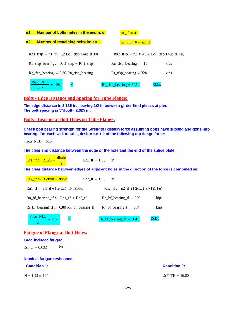
n1: Number of bolts holes in the end row n1_tf 4=
n2: Number of remaining bolts holes n2_tf 8 n1_tf−:=
Rn1_tfsp n1_tf 1.2 Lc1_tfsp⋅ Tout_tf⋅ Fu⋅( )⋅:= Rn2_tfsp n2_tf 1.2 Lc2_tfsp⋅ Tout_tf⋅ Fu⋅( )⋅:=
Rn_tfsp_bearing Rn1_tfsp Rn2_tfsp+:= Rn_tfsp_bearing 410= kips
Rr_tfsp_bearing 0.80 Rn_tfsp_bearing⋅:= Rr_tfsp_bearing 328= kips
Pncu_NLL2 2⋅
128= < Rr_tfsp_bearing 328= O.K.
Bolts - Edge Distance and Spacing for Tube Flange:The edge distance is 2.125 in., leaving 1/2 in between girder field pieces at pier.The bolt spacing is 3*dbolt= 2.625 in.
Bolts - Bearing at Bolt Holes on Tube Flange:
Check bolt bearing strength for the Strength I design force assuming bolts have slipped and gone intobearing. For each wall of tube, design for 1/2 of the following top flange force:
Pncu_NLL 513=
The clear end distance between the edge of the hole and the end of the splice plate:
Lc1_tf 2.125dhole
2−:= Lc1_tf 1.63= in
The clear distance between edges of adjacent holes in the direction of the force is computed as:
Lc2_tf 3 dbolt⋅ dhole−:= Lc2_tf 1.63= in
Rn1_tf n1_tf 1.2 Lc1_tf⋅ Tt1⋅ Fu⋅( )⋅:= Rn2_tf n2_tf 1.2 Lc2_tf⋅ Tt1⋅ Fu⋅( )⋅:=
Rn_bf_bearing_tf Rn1_tf Rn2_tf+:= Rn_bf_bearing_tf 380= kips
Rr_bf_bearing_tf 0.80 Rn_bf_bearing_tf⋅:= Rr_bf_bearing_tf 304= kips
Pncu_NLL2
257= = Rr_bf_bearing_tf 304= O.K.
Fatigue of Flange at Bolt Holes:Load-induced fatigue:
Δf_tf 0.032= ksi
Nominal fatigue resistance:
Condition 1: Condition 2:
N 1.23 108×= ΔF_TH 16.00=
B-25
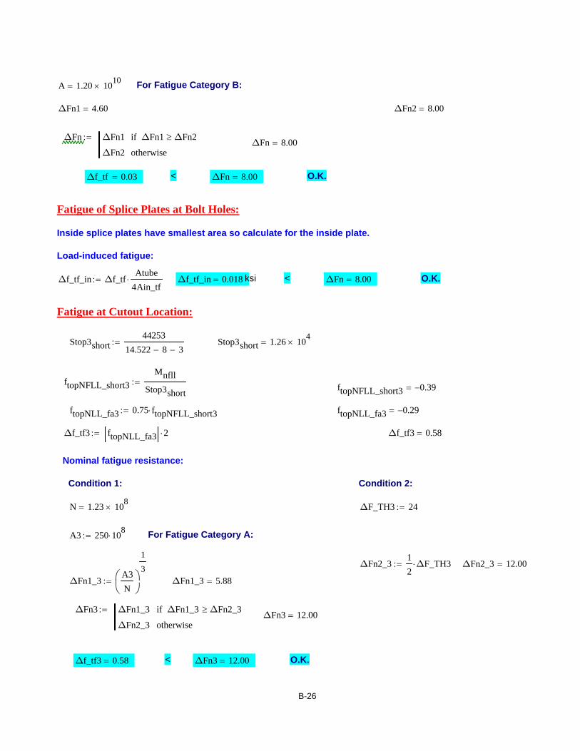
A 1.20 1010×= For Fatigue Category B:
ΔFn1 4.60= ΔFn2 8.00=
ΔFn ΔFn1 ΔFn1 ΔFn2≥if
ΔFn2 otherwise
:=ΔFn 8.00=
Δf_tf 0.03= < ΔFn 8.00= O.K.
Fatigue of Splice Plates at Bolt Holes:
Inside splice plates have smallest area so calculate for the inside plate.
Load-induced fatigue:
Δf_tf_in Δf_tfAtube
4Ain_tf⋅:= Δf_tf_in 0.018= ksi < ΔFn 8.00= O.K.
Fatigue at Cutout Location:
Stop3short44253
14.522 8− 3−:= Stop3short 1.26 104
×=
ftopNFLL_short3Mnfll
Stop3short:= ftopNFLL_short3 0.39−=
ftopNLL_fa3 0.75 ftopNFLL_short3⋅:= ftopNLL_fa3 0.29−=
Δf_tf3 ftopNLL_fa3 2⋅:= Δf_tf3 0.58=
Nominal fatigue resistance:
Condition 1: Condition 2:
N 1.23 108×= ΔF_TH3 24:=
A3 250 108⋅:= For Fatigue Category A:
ΔFn2_312
ΔF_TH3⋅:= ΔFn2_3 12.00=
ΔFn1_3A3N
⎛⎜⎝
⎞⎟⎠
1
3:= ΔFn1_3 5.88=
ΔFn3 ΔFn1_3 ΔFn1_3 ΔFn2_3≥if
ΔFn2_3 otherwise
:=ΔFn3 12.00=
Δf_tf3 0.58= < ΔFn3 12.00= O.K.
B-26

V. Compute Web Splice Design Loads (yellow highlight indicates input)
Girder Shear Forces at Splice Locations:DC1: Vdc1 0:= kip
DC2: Vdc2 0:= kip
DW: Vdw 0:= kip
LL(positive): Vpll 0:= kip
LL(negative): Vnll 0:= kip
Fatigue(positive): Vpfll 0:= kip
Fatigue(negative): Vnfll 0:= kip
Web Moments and Horizontal Force Resultant:Muw : Portion of the flexural moment assumed to be resisted by the webHuw : Horizontal design force resultantVuw : Design shear forceMuv : Moment due to the eccentricity of the design shear ( Muv = Vuw x e )e : Distance from the centerline of the splice to the centroid of the connection on the side of the joint
under considerationMtotal = Muw + Muv
e 2.375 2.625+:= e 5.00= in Based on three verical rows of bolts in each side
Strength I Limit State:Design Shear:The nominal shear resistance:
AvBwebTweb
:= Bv 1.1029000 5⋅
Fy⋅:= Cv 1.38
29000 5⋅Fy
⋅:=
Av 53.00= Bv 59.24= Cv 74.32=
Vp 0.58 Fy⋅ Bweb⋅ Tweb⋅:=
C 1.0 Av Bv<if
1.10Av
29000 5⋅Fy
⋅ Bv Av≤ Cv≤if
1.52
Av2
29000 5⋅Fy
⋅ Av Cv>if
:= : plastic
: inelastic
: elastic
C 1.00=
Vn C Vp⋅:= Vn 384.25= kip Vr 1 Vn⋅:= Vr 384.25= kip
The factored shear for the negative live load:
Vu_NLL 1.25 Vdc1⋅ 1.25 Vdc2⋅+ 1.5 Vdw⋅+ 1.75 Vnll⋅+( ) 0.95⋅:= Vu_NLL 0.00= kip
B-27

Therefore, with Vu Vu_NLL:= Vu 0.00= Vr 384.25=
AASHTO requires the following web splice design shear:
Vuw 0.75 Vr⋅ Vu 0.5 Vr⋅<if
Vu Vr+
2otherwise
:= Vuw 288.19= kip However, since web splice is over the bearing, set the design shear to zero:
Vuw 0:= kip
Web Moments and Horizontal Force Resultants:
Dead Load + Negative Live Load:fbotNLL_st 35.05−= ksi Maximum elastic flexural stress due to the factored loads at the
midthickness of the controlling flange
Fcf_NLL Fcf_NLL−:= Design stress for the controlling flange
Fcf_NLL 42.52−= ksi
ftopNLL_st 1.75−= ksi Maximum elastic flexural stress due to the factored loads at themidthickness of the noncontrolling flange
Rcf_NLL 1.21=
Portion of the flexural moment to be resisted by the web:
Mw_st_negTweb Bweb2
⋅
12Rh Fcf_NLL⋅ Rcf_NLL ftopNLL_st⋅−⋅:= Mw_st_neg 1.18 103
×= kip-in
Total web moment:
Mtot_st_neg Mw_st_neg Vuw e⋅+:= Mtot_st_neg 1.18 103×= kip-in
Horizontal force resultant:
Hw_st_negTweb Bweb⋅
2Rh Fcf_NLL⋅ Rcf_NLL ftopNLL_st⋅+( )⋅:= Hw_st_neg 295.78−= kip
Service II Limit State:Design Shear:The factored shear for the negative live load:
Vser_NLL 1.0 Vdc1⋅ 1.0 Vdc2⋅+ 1.0 Vdw⋅+ 1.3 Vnll⋅+:= Vser_NLL 0.00= kip
Therefore
Vw_ser Vser_NLL:= Vw_ser 0.00= kip
Web Moments and Horizontal Force Resultants:
Dead Load + Negative Live Load:fbotNLL_sv 24.22−= ksi Maximum Service II midthickness flange stress
ftopNLL_sv 0.30= ksi Service II midthickness flange stress in other flange
B-28

Portion of the flexural moment to be resisted by the web:
Mw_ser_negTweb Bweb2
⋅
12fbotNLL_sv ftopNLL_sv−⋅:= Mw_ser_neg 717.45= kip-in
Total web moment:
Mtot_ser_neg Mw_ser_neg Vw_ser e⋅+:= Mtot_ser_neg 717.45= kip-in
Horizontal force resultant:
Hw_ser_negTweb Bweb⋅
2fbotNLL_sv ftopNLL_sv+( )⋅:= Hw_ser_neg 158.51−= kip
Fatigue Limit State:Design Shear:The factored shear for the negative live load:
Vfat_NLL 0.75 Vnfll⋅:= Vfat_NLL 0.00= kip
Web Moments and Horizontal Force Resultants:
Negative Live Load:fbotNLL_fa 2.61−= ksi
ftopNLL_fa 0.03= ksi
Portion of the flexural moment to be resisted by the web:
Mw_fat_negTweb Bweb2
⋅
12fbotNLL_fa ftopNLL_fa−( )⋅:= Mw_fat_neg 77.43−= kip-in
Total web moment:
Mtot_fat_neg Mw_fat_neg Vfat_NLL e⋅+:= Mtot_fat_neg 77.43−= kip-in
Horizontal force resultant:
Hw_fat_negTweb Bweb⋅
2fbotNLL_fa ftopNLL_fa+( )⋅:= Hw_fat_neg 17.11−= kip
B-29

VI. Design Web Splice (yellow highlight indicates input)
Web Splice Configuration:
1. Three vertical rows of bolts with eight bolts per row.2. 1/2" x 21.5" splice plates on each side of the web.
twp12
:= dwp 21.5:=
Bolts - Minimum Spacing:dbolt 0.875= s_min 3 dbolt⋅:= s_min 2.625= in
Bolts - Edge Distance:
The smallest edge distance is 1.5in. and the bolt spacing is 3*dbolt= 2.625 in.
Bolts - Shear:
m 3:= : Number of vertical rows of bolts
n 8:= : Number of bolts in one verical row
s 2.625:= in : Vertical pitch
g 2.625:= in : Horizontal pitch
Ipn m⋅12
s2 n2 1−( )⋅ g2 m2 1−( )⋅+⎡⎣ ⎤⎦⋅:= Ip 978.47= in2 : Polar moment of inertia
Nbw n m⋅:= Nbw 24.00= : Total number of web bolts on each sideof the splice
Strength I Limit State:
Assume that the threads are excluded from the shear planes
Ru_web Ru_tf:= Ru_web 55.42= kip
Dead Load + Negative Live Load:
Vuw 0.00= kip Mtot_st_neg 1.18 103×= kip-in Hw_st_neg 295.78−= kip
Vertical shear force in the bolts due to applied shear force:
Pv_stVuwNbw
:= Pv_st 0.00= kip
Horizontal shear force in the bolts due to horizontal force resultant:
Ph_st_negHw_st_neg
Nbw:= Ph_st_neg 12.32= kip
B-30

Horizontal and vertical components of the bolt shear force on the extreme bolt due to the total moment inthe web:
xg2
:= x 1.31= in y15 s⋅
2:= y 19.69= in
Pmv_st_negMtot_st_neg x⋅
Ip:= Pmv_st_neg 1.59= kip
Pmh_st_negMtot_st_neg y⋅
Ip:= Pmh_st_neg 23.79= kip
Pr_st_neg Pv_st Pmv_st_neg+( )2 Ph_st_neg Pmh_st_neg+( )2+:= Pr_st_neg 36.15=
Pr_st Pr_st_neg:=
Pr_st 36.15= < Ru_web 55.42= O.K.
Service II Limit State:
Determine the factored resistance per bolt assuming a Class B surface condition.
Rr_slip_web Rr_slip_tf:= Rr_slip_web 39.00= kip
Dead Load + Negative Live Load:
Vw_ser 0.00= kip Mtot_ser_neg 717.45= kip-in Hw_ser_neg 158.51−= kip
Vertical shear force in the bolts due to applied shear force:
Ps_serVw_ser
Nbw:= Ps_ser 0.00= kip
Horizontal shear force in the bolts due to horizontal force resultant:
Ph_ser_negHw_ser_neg
Nbw:= Ph_ser_neg 6.60= kip
Horizontal and vertical components of the bolt shear force on the extreme bolt due to the total moment inthe web:
Pmv_ser_negMtot_ser_neg x⋅
Ip:= Pmv_ser_neg 0.96= kip
Pmh_ser_negMtot_ser_neg y⋅
Ip:= Pmh_ser_neg 14.44= kip
Pr_ser_neg Ps_ser Pmv_ser_neg+( )2 Ph_ser_neg Pmh_ser_neg+( )2+:= Pr_ser_neg 21.06= kip
Pr_ser Pr_ser_neg:=
Pr_ser 21.06= < Rr_slip_web 39.00= O.K.
B-31

Shear Yielding of Splice Plates:Vuw 0.00= kip
Nwp 2:= : Number of splice plates
twp 0.50= in : Thickness of splice plate
dwp 21.50= in : Depth of splice plate
Agross_wp Nwp twp⋅ dwp⋅:= Agross_wp 21.50= in2
Rr_wp 0.58 Fy⋅ Agross_wp⋅:= Rr_wp 623.50= kip
Vuw 0.00= < Rr_wp 623.50= O.K.
Fracture of Splice Plates:
Nfn n:= Nfn 8.00= : Number of bolts along one plane
Avn Nwp dwp Nfn dhole⋅−( )⋅ twp⋅:= Avn 13.50= in2
A85 0.85 Agross_wp⋅:= A85 18.27= in2
Avn 13.50= < A85 18.27= O.K.
Rr_web_fra 0.80 0.58 Fu⋅ Avn⋅( )⋅:=
Vuw 0.00= < Rr_web_fra 407.16= O.K.
Flexural Yielding of Splice Plates:
Sp116
Agross_wp⋅ dwp⋅:= Sp1 77.04= in3
Mtot_st_neg 1.18 103×= kip-in Hw_st_neg 295.78−= kip
fst_negMtot_st_neg
Sp1Hw_st_negAgross_wp
+:= fst_neg 29.10= ksi
fst_neg 29.10= < Fy 50.00= O.K.
B-32

Bolts - Bearing at Bolt Holes in Splice Plate:
The clear distance between the edge of the hole and the edge of the splice plate:
Lc1_web_sp 1.5dhole
2−:= Lc1_web_sp 1.00= in
The clear distance between holes:
Lc2_web_sp 3.0 dbolt⋅ dhole−:= Lc2_web_sp 1.63= in
The clear distance to edge of plate controls.
Rn_web_sp_bearing 1.2 Lc1_web_sp⋅ twp⋅ Fu⋅:= Rn_web_sp_bearing 39.00= kips
Rr_web_sp_bearing 0.80 Rn_web_sp_bearing⋅:= Rr_web_sp_bearing 31.20= kips
Pr_st2
18.07= < Rr_web_sp_bearing 31.20= O.K.
Bolts - Bearing at Bolt Holes in Web:The edge distance is 2.125 in., leaving 1/2 in between girder field pieces at pier.The bolt spacing is 3*dbolt= 2.625 in.
The clear distance between the edge of the hole and the edge of the girder:
Lc1_web 2.125dhole
2−:= Lc1_web 1.63= in
The clear distance between holes:
Lc2_web 3.0 dbolt⋅ dhole−:= Lc2_web 1.63= in
The two clear distances are the same.
Rn_web_bearing 1.2 Lc1_web⋅ Tweb⋅ Fu⋅:= Rn_web_bearing 63.38= kips
Rr_web_bearing 0.80 Rn_web_bearing⋅:= Rr_web_bearing 50.70= kips
Pr_st 36.15= = Rr_web_bearing 50.70= O.K.
Fatigue of Splice Plates:
Nominal stresses at the bottom edge of the splice plates due to the total positive and negative fatigue-loadweb moments and the coresponding horizontal force resultants:
Case 2 - Negative Live Load:
Mtot_fat_neg 77.43−= kip-in Hw_fat_neg 17.11−= kip
ffat_negMtot_fat_neg
Sp1Hw_fat_negAgross_wp
+:= ffat_neg 1.80−= ksi Δf_w_sp ffat_neg:= Δf_w_sp 1.80=
Δf_w_sp 1.80= < ΔFn 8.00= O.K.
B-33

Appendix C. Plastic Moment for Composite Section
1. Procedure- Calculate the axial force and the moment of the rectangular CFT flange part including the slab interms of the plastic neutral axis (PNA).
- Combine those results with compression or tension forces of the web and flat tension flange in termsof the PNA.
- Determine the location of the PNA, referenced from the top of the concrete slab, by the equilibrium condition.
- Calculate the plastic moment.
2. Properties and Dimensions (yellow highlight indicates input data)BRIDGE PARAMETERS
Description: Two span continuous (for superimposed dead load and live load) composite CFTFG with each span of100 ft and width of 31 ft - 4.5 in. The bridge has 4 girders spaced at 8 ft - 5.5 in with 3 ft overhangs.
Bridge Width (in) Bridge Span Length (in) Slab Thickness (in) Haunch Thickness (in) Girder Spacing (in)
W 376.5:= L 1200:= Tslab 8:= Thaunch 3:= s 101.5:=
Number of Girders Overhang (from girder centerline) (in) Combined Slab and Haunch Thickness (in)
ng 4:= se 36:= Tconc Tslab Thaunch+:= Tconc 11=
MATERIAL PROPERTIES
Yield Strength (ksi) Young's Modulus (ksi) Concrete Strength (ksi) Modular ratio (input)
Fy 50:= E 29000:= fc 4:= n 8:=
Yield Strain (ksi) Concrete Modulus (ksi) Concrete StressBlock Parameter
Max. Concrete Strain Modular ratio (actual)
εyFyE
:= Ec57000 fc 1000⋅⋅
1000:= β1 0.85:= εuslab 0.003:=
EEc
8.04=
STEEL GIRDER DIMENSIONS
Tube horizontal platethickness
Tube vertical platethickness
Bottom flangethickness
Webthickness
Tt138
:= inches Tt238
:= inches Tbf 1.5:= inches Tweb816
:= inches
Tube horizontal platewidth
Tube vertical platewidth
Bottom flangewidth
Bt1 16:= inches Bt2 7.25:= inches Bbf 18:= inches
Web depth Dweb 36 2 Tt1⋅− Bt2− Tbf−:= Dweb 26.5= inches
Total girder depth Dgirder Tbf Dweb+ 2 Tt1⋅+ Bt2+:= Dgirder 36= inches
Depth including deck Dtotal Dgirder Thaunch+ Tslab+:= Dtotal 47= inches
C-1
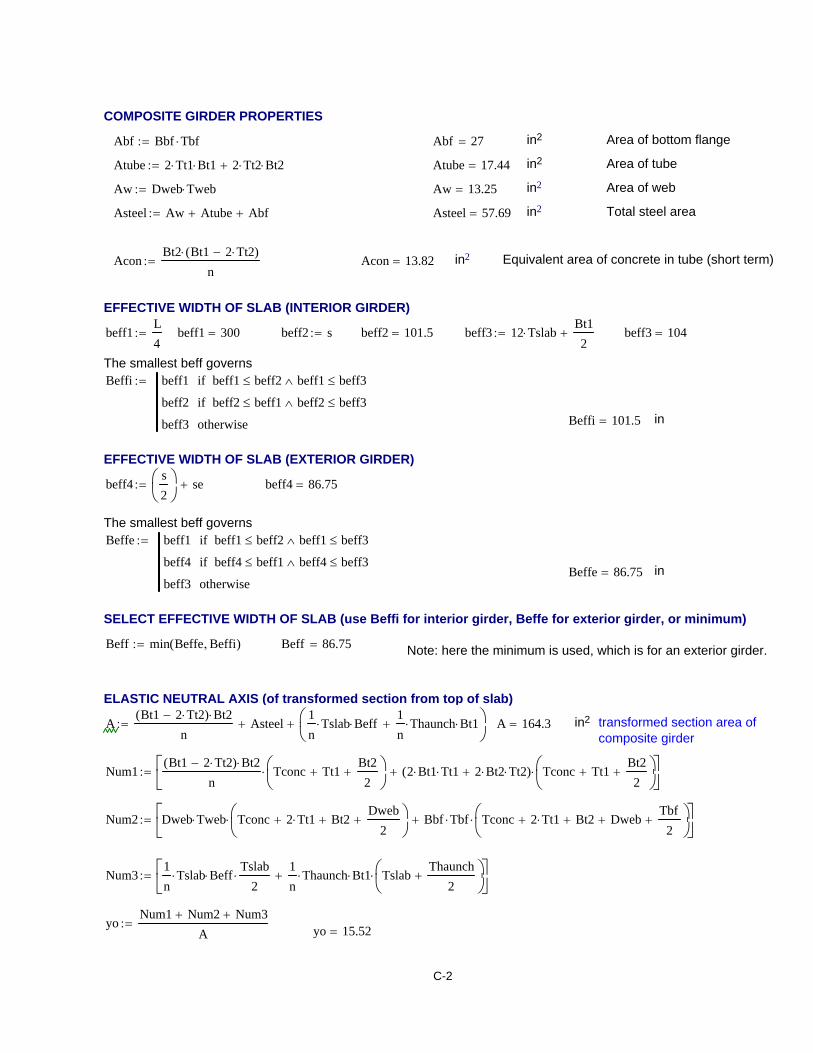
COMPOSITE GIRDER PROPERTIES
Abf Bbf Tbf⋅:= Abf 27= in2 Area of bottom flange
Atube 2 Tt1⋅ Bt1⋅ 2 Tt2⋅ Bt2⋅+:= Atube 17.44= in2 Area of tube
Aw Dweb Tweb⋅:= Aw 13.25= in2 Area of web
Asteel Aw Atube+ Abf+:= Asteel 57.69= in2 Total steel area
AconBt2 Bt1 2 Tt2⋅−( )⋅
n:= Acon 13.82= in2 Equivalent area of concrete in tube (short term)
EFFECTIVE WIDTH OF SLAB (INTERIOR GIRDER)
beff1L4
:= beff1 300= beff2 s:= beff2 101.5= beff3 12 Tslab⋅Bt12
+:= beff3 104=
The smallest beff governsBeffi beff1 beff1 beff2≤ beff1 beff3≤∧if
beff2 beff2 beff1≤ beff2 beff3≤∧if
beff3 otherwise
:=
Beffi 101.5= in
EFFECTIVE WIDTH OF SLAB (EXTERIOR GIRDER)
beff4s2
⎛⎜⎝
⎞⎟⎠
se+:= beff4 86.75=
The smallest beff governsBeffe beff1 beff1 beff2≤ beff1 beff3≤∧if
beff4 beff4 beff1≤ beff4 beff3≤∧if
beff3 otherwise
:=
Beffe 86.75= in
SELECT EFFECTIVE WIDTH OF SLAB (use Beffi for interior girder, Beffe for exterior girder, or minimum)
Beff min Beffe Beffi, ( ):= Beff 86.75= Note: here the minimum is used, which is for an exterior girder.
ELASTIC NEUTRAL AXIS (of transformed section from top of slab)
ABt1 2 Tt2⋅−( ) Bt2⋅
nAsteel+
1n
Tslab⋅ Beff⋅1n
Thaunch⋅ Bt1⋅+⎛⎜⎝
⎞⎟⎠
+:= A 164.3= in2 transformed section area ofcomposite girder
Num1Bt1 2 Tt2⋅−( ) Bt2⋅
nTconc Tt1+
Bt22
+⎛⎜⎝
⎞⎟⎠
⋅ 2 Bt1⋅ Tt1⋅ 2 Bt2⋅ Tt2⋅+( ) Tconc Tt1+Bt22
+⎛⎜⎝
⎞⎟⎠
⋅+⎡⎢⎣
⎤⎥⎦
:=
Num2 Dweb Tweb⋅ Tconc 2 Tt1⋅+ Bt2+Dweb
2+⎛⎜
⎝⎞⎟⎠
⋅ Bbf Tbf⋅ Tconc 2 Tt1⋅+ Bt2+ Dweb+Tbf2
+⎛⎜⎝
⎞⎟⎠
⋅+⎡⎢⎣
⎤⎥⎦
:=
Num31n
Tslab⋅ Beff⋅Tslab
2⋅
1n
Thaunch⋅ Bt1⋅ TslabThaunch
2+⎛⎜
⎝⎞⎟⎠
⋅+⎡⎢⎣
⎤⎥⎦
:=
yoNum1 Num2+ Num3+
A:= yo 15.52=
C-2

COORDINATES OF CROSS-SECTION ELEMENTS:
Coordinates denoted with "a" are taken from center of CFT compression flange. Upward is positive
a1 Tslab Thaunch+ Tt1+Bt22
+:= : top face of slab
a2 Thaunch Tt1+Bt22
+:= : bottom face of slab
a3 Tt1Bt22
+:= : outer face of top plate of steel tube
a4Bt22
:= : inner face of top plate of steel tube
a5 a4−:= : inner face of bottom plate of steel tube
a6 a3−:= : outer face of bottom plate of steel tube
a7 c( ) a1 c−:= : plastic neutral axis (PNA) relative to center of tube (positive indicates PNA is above center of tube)
a8 c( ) a1 β1 c⋅−:= : bottom edge of concrete stress block
a9 c( ) a1 c−εy
εuslabc⋅−:= : location where yield strain is reached in tension zone
of steel ( used for tube )
a10 c( ) a1 c−εy
εuslabc⋅+:= : location where yield strain is reached in compression
zone of steel ( used for tube )
Coordinates denoted with "g" are taken from elastic neutral axis (ENA) of section. Upward is positive.
g1 yo Tconc− 2 Tt1⋅ Bt2+( )−:= : top edge of web
g2 yo Tconc− 2 Tt1⋅ Bt2+( )− Dweb−:= : bottom edge of web
g3 yo Tconc− 2 Tt1⋅ Bt2+( )− Dweb− Tbf−:= : bottom face of tension flange
g4 c( ) yo c−εy
εuslabc⋅−:= : location where yield strain is reached in tension zone
of steel ( used for web )
g5 c( ) yo c−εy
εuslabc⋅+:= : location where yield strain is reached in compression
zone of steel ( used for web )
g6 c( ) yo c−:= : plastic neutral axis (PNA) relative to ENA (positive indicates PNA is above ENA)
Functions denoted with "z" give the variation of stress with position on cross section.
z1 c y, ( )y a7 c( )−
a10 c( ) a7 c( )−Fy⋅:= : stress variations about center of CFT flange
(compression is positive, used for tube)
z2 c y, ( )c yo− y+
c yo− g5 c( )+Fy⋅:= : stress variations about ENA
(compression is positive, used for web)
C-3

3. Assume PNA is in Slab or Haunch
3-1. Rectangular CFT Compression Flange and Deck
Deck
Pcon c( )a8 c( )
a1y0.85 fc⋅ Beff⋅
⌠⎮⌡
d a8 c( ) a2>if
a2
a1y0.85 fc⋅ Beff⋅
⌠⎮⌡
d a8 c( ) a2≤if
:= Mcon c( )a8 c( )
a1y0.85 fc⋅ Beff⋅ y⋅
⌠⎮⌡
d a8 c( ) a2>if
a2
a1y0.85 fc⋅ Beff⋅ y⋅
⌠⎮⌡
d a8 c( ) a2≤if
:=
Top plate of tubePuptube c( )
a4
a3yBt1− Fy⋅
⌠⎮⌡
d a9 c( ) a3>if
a9 c( )
a3yBt1 z1 c y, ( )⋅
⌠⎮⌡
da4
a9 c( )yBt1− Fy⋅
⌠⎮⌡
d+ a4 a9 c( )< a3≤if
a4
a3yBt1 z1 c y, ( )⋅
⌠⎮⌡
d a9 c( ) a4≤if
:=
Muptube c( )a4
a3yBt1− Fy⋅ y⋅
⌠⎮⌡
d a9 c( ) a3>if
a9 c( )
a3yBt1 z1 c y, ( )⋅ y⋅
⌠⎮⌡
da4
a9 c( )yBt1− Fy⋅ y⋅
⌠⎮⌡
d+ a4 a9 c( )< a3≤if
a4
a3yBt1 z1 c y, ( )⋅ y⋅
⌠⎮⌡
d a9 c( ) a4≤if
:=
Side plates of tubePmidtube c( )
a5
a4y2− Tt2⋅ Fy⋅
⌠⎮⌡
d a9 c( ) a4>if
a9 c( )
a4y2 Tt2⋅ z1 c y, ( )⋅
⌠⎮⌡
da5
a9 c( )y2− Tt2⋅ Fy⋅
⌠⎮⌡
d+ a5 a9 c( )< a4≤if
a4
a3y2 Tt2⋅ z1 c y, ( )⋅
⌠⎮⌡
d a9 c( ) a5≤if
:=
C-4
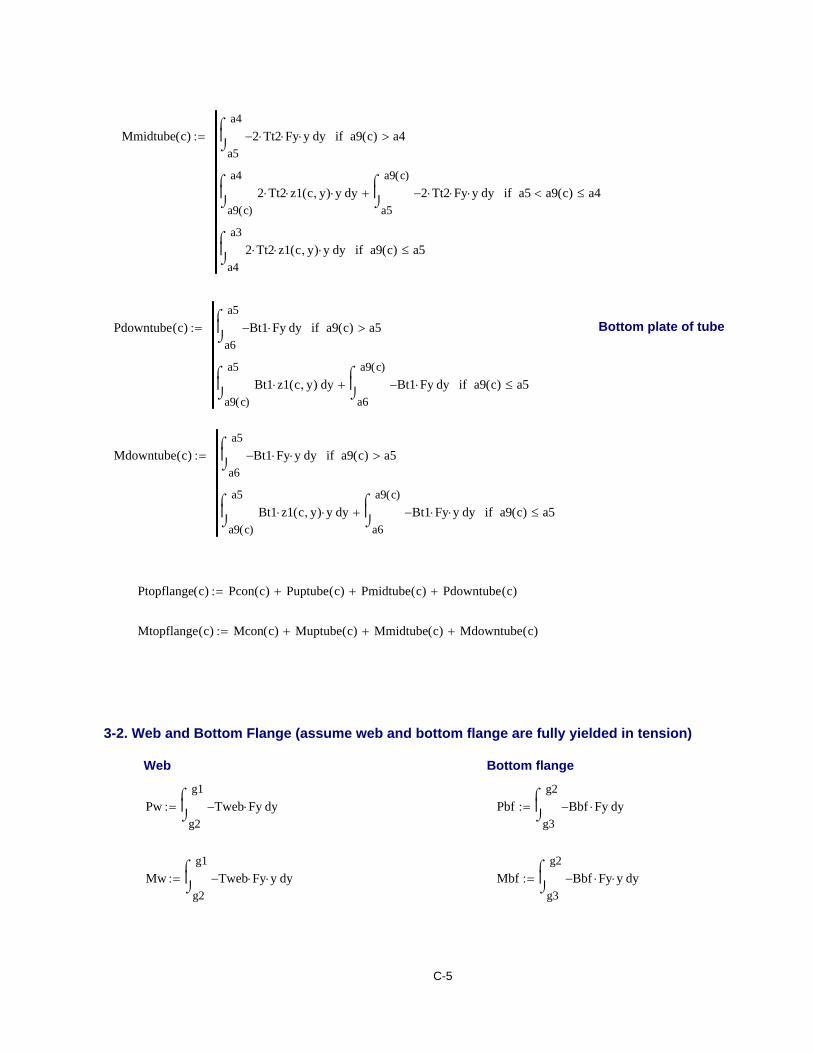
Mmidtube c( )a5
a4y2− Tt2⋅ Fy⋅ y⋅
⌠⎮⌡
d a9 c( ) a4>if
a9 c( )
a4y2 Tt2⋅ z1 c y, ( )⋅ y⋅
⌠⎮⌡
da5
a9 c( )y2− Tt2⋅ Fy⋅ y⋅
⌠⎮⌡
d+ a5 a9 c( )< a4≤if
a4
a3y2 Tt2⋅ z1 c y, ( )⋅ y⋅
⌠⎮⌡
d a9 c( ) a5≤if
:=
Pdowntube c( )a6
a5yBt1− Fy⋅
⌠⎮⌡
d a9 c( ) a5>if
a9 c( )
a5yBt1 z1 c y, ( )⋅
⌠⎮⌡
da6
a9 c( )yBt1− Fy⋅
⌠⎮⌡
d+ a9 c( ) a5≤if
:= Bottom plate of tube
Mdowntube c( )a6
a5yBt1− Fy⋅ y⋅
⌠⎮⌡
d a9 c( ) a5>if
a9 c( )
a5yBt1 z1 c y, ( )⋅ y⋅
⌠⎮⌡
da6
a9 c( )yBt1− Fy⋅ y⋅
⌠⎮⌡
d+ a9 c( ) a5≤if
:=
Ptopflange c( ) Pcon c( ) Puptube c( )+ Pmidtube c( )+ Pdowntube c( )+:=
Mtopflange c( ) Mcon c( ) Muptube c( )+ Mmidtube c( )+ Mdowntube c( )+:=
3-2. Web and Bottom Flange (assume web and bottom flange are fully yielded in tension)
Web Bottom flange
Pwg2
g1yTweb− Fy⋅
⌠⎮⌡
d:= Pbfg3
g2yBbf− Fy⋅
⌠⎮⌡
d:=
Mwg2
g1yTweb− Fy⋅ y⋅
⌠⎮⌡
d:= Mbfg3
g2yBbf− Fy⋅ y⋅
⌠⎮⌡
d:=
C-5
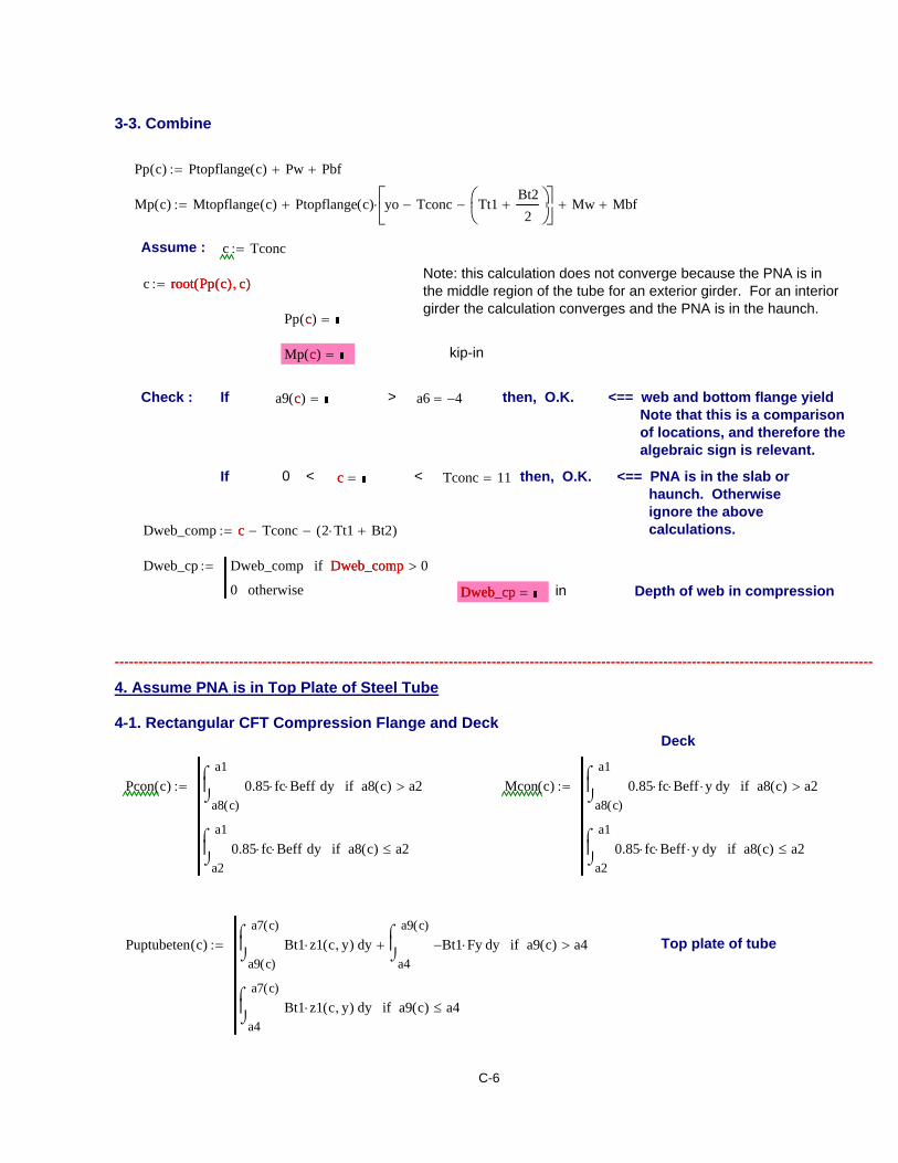
3-3. Combine
Pp c( ) Ptopflange c( ) Pw+ Pbf+:=
Mp c( ) Mtopflange c( ) Ptopflange c( ) yo Tconc− Tt1Bt22
+⎛⎜⎝
⎞⎟⎠
−⎡⎢⎣
⎤⎥⎦
⋅+ Mw+ Mbf+:=
Assume : c Tconc:=
Note: this calculation does not converge because the PNA is inthe middle region of the tube for an exterior girder. For an interiorgirder the calculation converges and the PNA is in the haunch.
c root Pp c( ) c, ( ):= root Pp c( ) c, ( )
Pp c( ) =c
Mp c( ) =c kip-in
Check : If a9 c( ) =c > a6 4−= then, O.K. <== web and bottom flange yield Note that this is a comparison of locations, and therefore the algebraic sign is relevant.
If 0 < c =c < Tconc 11= then, O.K. <== PNA is in the slab or haunch. Otherwise ignore the above calculations. Dweb_comp c Tconc− 2 Tt1⋅ Bt2+( )−:= c
Dweb_cp Dweb_comp Dweb_comp 0>if
0 otherwise
:= Dweb_comp
Dweb_cp =Dweb_cp in Depth of web in compression
---------------------------------------------------------------------------------------------------------------------------------------------------------------
4. Assume PNA is in Top Plate of Steel Tube
4-1. Rectangular CFT Compression Flange and DeckDeck
Pcon c( )a8 c( )
a1y0.85 fc⋅ Beff⋅
⌠⎮⌡
d a8 c( ) a2>if
a2
a1y0.85 fc⋅ Beff⋅
⌠⎮⌡
d a8 c( ) a2≤if
:= Mcon c( )a8 c( )
a1y0.85 fc⋅ Beff⋅ y⋅
⌠⎮⌡
d a8 c( ) a2>if
a2
a1y0.85 fc⋅ Beff⋅ y⋅
⌠⎮⌡
d a8 c( ) a2≤if
:=
Puptubeten c( )a9 c( )
a7 c( )yBt1 z1 c y, ( )⋅
⌠⎮⌡
da4
a9 c( )yBt1− Fy⋅
⌠⎮⌡
d+ a9 c( ) a4>if
a4
a7 c( )yBt1 z1 c y, ( )⋅
⌠⎮⌡
d a9 c( ) a4≤if
:= Top plate of tube
C-6

Muptubeten c( )a9 c( )
a7 c( )yBt1 z1 c y, ( )⋅ y⋅
⌠⎮⌡
da4
a9 c( )yBt1− Fy⋅ y⋅
⌠⎮⌡
d+ a9 c( ) a4>if
a4
a7 c( )yBt1 z1 c y, ( )⋅ y⋅
⌠⎮⌡
d a9 c( ) a4≤if
:=
Puptubecom c( )a7 c( )
a3yBt1 z1 c y, ( )⋅
⌠⎮⌡
d:= Muptubecom c( )a7 c( )
a3yBt1 z1 c y, ( )⋅ y⋅
⌠⎮⌡
d:=
Puptube c( ) Puptubeten c( ) Puptubecom c( )+:= Muptube c( ) Muptubeten c( ) Muptubecom c( )+:=
Pmidtube c( )a5
a4y2− Tt2⋅ Fy⋅
⌠⎮⌡
d a9 c( ) a4>if
a9 c( )
a4y2 Tt2⋅ z1 c y, ( )⋅
⌠⎮⌡
da5
a9 c( )y2− Tt2⋅ Fy⋅
⌠⎮⌡
d+ a5 a9 c( )< a4≤if
a5
a4y2 Tt2⋅ z1 c y, ( )⋅
⌠⎮⌡
d a9 c( ) a5≤if
:= Side plates of tube
Mmidtube c( )a5
a4y2− Tt2⋅ Fy⋅ y⋅
⌠⎮⌡
d a9 c( ) a4>if
a9 c( )
a4y2 Tt2⋅ z1 c y, ( )⋅ y⋅
⌠⎮⌡
da5
a9 c( )y2− Tt2⋅ Fy⋅ y⋅
⌠⎮⌡
d+ a5 a9 c( )< a4≤if
a5
a4y2 Tt2⋅ z1 c y, ( )⋅ y⋅
⌠⎮⌡
d a9 c( ) a5≤if
:=
Pdowntube c( )a6
a5yBt1− Fy⋅
⌠⎮⌡
d a9 c( ) a5>if
a9 c( )
a5yBt1 z1 c y, ( )⋅
⌠⎮⌡
da6
a9 c( )yBt1− Fy⋅
⌠⎮⌡
d+ a6 a9 c( )< a5≤if
a6
a5yBt1 z1 c y, ( )⋅
⌠⎮⌡
d a9 c( ) a6<if
:= Bottom plate of tube
C-7

Mdowntube c( )a6
a5yBt1− Fy⋅ y⋅
⌠⎮⌡
d a9 c( ) a5>if
a9 c( )
a5yBt1 z1 c y, ( )⋅ y⋅
⌠⎮⌡
da6
a9 c( )yBt1− Fy⋅ y⋅
⌠⎮⌡
d+ a6 a9 c( )< a5≤if
a6
a5yBt1 z1 c y, ( )⋅ y⋅
⌠⎮⌡
d a9 c( ) a6<if
:=
Ptopflange c( ) Pcon c( ) Puptube c( )+ Pmidtube c( )+ Pdowntube c( )+:=
Mtopflange c( ) Mcon c( ) Muptube c( )+ Mmidtube c( )+ Mdowntube c( )+:=
4-2. Web and Bottom Flange (assume web and bottom flange are fully yielded in tension)Web Bottom flange
Pwg2
g1yTweb− Fy⋅
⌠⎮⌡
d:= Pbfg3
g2yBbf− Fy⋅
⌠⎮⌡
d:=
Mwg2
g1yTweb− Fy⋅ y⋅
⌠⎮⌡
d:= Mbfg3
g2yBbf− Fy⋅ y⋅
⌠⎮⌡
d:=
4-3. Combine
Pp c( ) Ptopflange c( ) Pw+ Pbf+:=
Mp c( ) Mtopflange c( ) Ptopflange c( ) yo Tconc− Tt1Bt22
+⎛⎜⎝
⎞⎟⎠
−⎡⎢⎣
⎤⎥⎦
⋅+ Mw+ Mbf+:=
Assume : c Tconc:=
c root Pp c( ) c, ( ):= c 12.21= Note: this calculation does not control because the PNA isin the middle tube region for an exterior girder. For aninterior girder the PNA is in the haunch.Pp c( ) 2.27− 10 13−
×=
Mp c( ) 8.1 104×= kip-in
Check : If a9 c( ) 4.22−= > a6 4−= then, O.K. <== web and bottom flange yield
If Tconc 11= < c 12.21= < Tconc Tt1+ 11.38= then, O.K.
<== PNA is in the top of the steel tube. Otherwise ignore the above calculations.
Dweb_comp c Tconc− 2 Tt1⋅ Bt2+( )−:=
Dweb_cp Dweb_comp Dweb_comp 0>if
0 otherwise
:=
Dweb_cp 0= in Depth of web in compression
C-8

---------------------------------------------------------------------------------------------------------------------------------------------------------------
5. Assume PNA is in Middle Region of Steel Tube
5-1. Rectangular CFT Compression Flange and Deck
Deck and concrete in tubePcon c( )
a8 c( )
a1y0.85 fc⋅ Beff⋅
⌠⎮⌡
d a8 c( ) a2>if
a2
a1y0.85 fc⋅ Beff⋅
⌠⎮⌡
d a4 a8 c( )< a2≤if
a2
a1y0.85 fc⋅ Beff⋅
⌠⎮⌡
da8 c( )
a4y0.85 fc⋅ Bt1 2 Tt2⋅−( )⋅
⌠⎮⌡
d+ a8 c( ) a4≤if
:=
Mcon c( )a8 c( )
a1y0.85 fc⋅ Beff⋅ y⋅
⌠⎮⌡
d a8 c( ) a2>if
a2
a1y0.85 fc⋅ Beff⋅ y⋅
⌠⎮⌡
d a4 a8 c( )< a2≤if
a2
a1y0.85 fc⋅ Beff⋅ y⋅
⌠⎮⌡
da8 c( )
a4y0.85 fc⋅ Bt1 2 Tt2⋅−( )⋅ y⋅
⌠⎮⌡
d+ a8 c( ) a4≤if
:=
Puptube c( )a4
a3yBt1 z1 c y, ( )⋅
⌠⎮⌡
d a10 c( ) a3>if
a10 c( )
a3yBt1 Fy⋅
⌠⎮⌡
da4
a10 c( )yBt1 z1 c y, ( )⋅
⌠⎮⌡
d+ a4 a10 c( )< a3≤if
a4
a3yBt1 Fy⋅
⌠⎮⌡
d a10 c( ) a4≤if
:= Top plate of tube
Muptube c( )a4
a3yBt1 z1 c y, ( )⋅ y⋅
⌠⎮⌡
d a10 c( ) a3>if
a10 c( )
a3yBt1 Fy⋅ y⋅
⌠⎮⌡
da4
a10 c( )yBt1 z1 c y, ( )⋅ y⋅
⌠⎮⌡
d+ a4 a10 c( )< a3≤if
a4
a3yBt1 Fy⋅ y⋅
⌠⎮⌡
d a10 c( ) a4≤if
:=
C-9

Side plates of tubePmidtubeten c( )
a9 c( )
a7 c( )y2 Tt2⋅ z1 c y, ( )⋅
⌠⎮⌡
da5
a9 c( )y2− Tt2⋅ Fy⋅
⌠⎮⌡
d+ a9 c( ) a5≥if
a5
a7 c( )y2 Tt2⋅ z1 c y, ( )⋅
⌠⎮⌡
d a9 c( ) a5<if
:=
Mmidtubeten c( )a9 c( )
a7 c( )y2 Tt2⋅ z1 c y, ( )⋅ y⋅
⌠⎮⌡
da5
a9 c( )y2− Tt2⋅ Fy⋅ y⋅
⌠⎮⌡
d+ a9 c( ) a5≥if
a5
a7 c( )y2 Tt2⋅ z1 c y, ( )⋅ y⋅
⌠⎮⌡
d a9 c( ) a5<if
:=
Pmidtubecom c( )a7 c( )
a4y2 Tt2⋅ z1 c y, ( )⋅
⌠⎮⌡
d a10 c( ) a4>if
a10 c( )
a4y2 Tt2⋅ Fy⋅
⌠⎮⌡
da7 c( )
a10 c( )y2 Tt2⋅ z1 c y, ( )⋅
⌠⎮⌡
d+ a10 c( ) a4≤if
:=
Mmidtubecom c( )a7 c( )
a4y2 Tt2⋅ z1 c y, ( )⋅ y⋅
⌠⎮⌡
d a10 c( ) a4>if
a10 c( )
a4y2 Tt2⋅ Fy⋅ y⋅
⌠⎮⌡
da7 c( )
a10 c( )y2 Tt2⋅ z1 c y, ( )⋅ y⋅
⌠⎮⌡
d+ a10 c( ) a4≤if
:=
Pmidtube c( ) Pmidtubeten c( ) Pmidtubecom c( )+:= Mmidtube c( ) Mmidtubeten c( ) Mmidtubecom c( )+:=
Pdowntube c( )a6
a5yBt1− Fy⋅
⌠⎮⌡
d a9 c( ) a5>if
a9 c( )
a5yBt1 z1 c y, ( )⋅
⌠⎮⌡
da6
a9 c( )yBt1− Fy⋅
⌠⎮⌡
d+ a6 a9 c( )< a5≤if
a6
a5yBt1 z1 c y, ( )⋅
⌠⎮⌡
d a9 c( ) a6<if
:= Bottom plate of tube
Mdowntube c( )a6
a5yBt1− Fy⋅ y⋅
⌠⎮⌡
d a9 c( ) a5>if
a9 c( )
a5yBt1 z1 c y, ( )⋅ y⋅
⌠⎮⌡
da6
a9 c( )yBt1− Fy⋅ y⋅
⌠⎮⌡
d+ a6 a9 c( )< a5≤if
a6
a5yBt1 z1 c y, ( )⋅ y⋅
⌠⎮⌡
d a9 c( ) a6<if
:=
C-10

Ptopflange c( ) Pcon c( ) Puptube c( )+ Pmidtube c( )+ Pdowntube c( )+:=
Mtopflange c( ) Mcon c( ) Muptube c( )+ Mmidtube c( )+ Mdowntube c( )+:=
5-2. Web and Bottom Flange (assume bottom flange is fully yielded in tension, but check web)Web Bottom flange
Pw c( )g2
g1yTweb− Fy⋅
⌠⎮⌡
d g4 c( ) g1≥if
g4 c( )
g1yTweb z2 c y, ( )⋅
⌠⎮⌡
dg2
g4 c( )yTweb− Fy⋅
⌠⎮⌡
d+ g4 c( ) g1<if
:=Pbf
g3
g2yBbf− Fy⋅
⌠⎮⌡
d:=
Mbfg3
g2yBbf− Fy⋅ y⋅
⌠⎮⌡
d:=Mw c( )g2
g1yTweb− Fy⋅ y⋅
⌠⎮⌡
d g4 c( ) g1≥if
g4 c( )
g1yTweb z2 c y, ( )⋅ y⋅
⌠⎮⌡
dg2
g4 c( )yTweb− Fy⋅ y⋅
⌠⎮⌡
d+ g4 c( ) g1<if
:=
5-3. Combine
Pp c( ) Ptopflange c( ) Pw c( )+ Pbf+:=
Mp c( ) Mtopflange c( ) Ptopflange c( ) yo Tconc− Tt1Bt22
+⎛⎜⎝
⎞⎟⎠
−⎡⎢⎣
⎤⎥⎦
⋅+ Mw c( )+ Mbf+:=
Assume : c Tconc Tt1+:=
c root Pp c( ) c, ( ):= c 12.21=Note: this calculation contols for an exterior girder.For an interior girder the PNA is in the haunch.Pp c( ) 2.27 10 13−
×=
Mp c( ) 8.0985 104×= kip-in
Check : If g4 c( ) 3.7−= > g2 29.98−= then, O.K. <== bottom flange is fully yielded
If Tconc Tt1+ 11.38= < c 12.21= < Tconc Tt1+ Bt2+ 18.63= then, O.K.
<== PNA is in the middle region of the steel tube. Otherwise ignore the above calculations.
Dweb_comp c Tconc− 2 Tt1⋅ Bt2+( )−:=
Dweb_cp Dweb_comp Dweb_comp 0>if
0 otherwise
:=
Dweb_cp 0= in Depth of web in compression
C-11

---------------------------------------------------------------------------------------------------------------------------------------------------------------
6. Assume PNA is in Bottom of Steel Tube
6-1. Rectangular CFT Compression Flange Part Deck and concrete in tube(assumes β*c>a2, check later)
Pcon c( )a2
a1y0.85 fc⋅ Beff⋅
⌠⎮⌡
da8 c( )
a4y0.85 fc⋅ Bt1 2 Tt2⋅−( )⋅
⌠⎮⌡
d+ a8 c( ) a5≥if
a2
a1y0.85 fc⋅ Beff⋅
⌠⎮⌡
da5
a4y0.85 fc⋅ Bt1 2 Tt2⋅−( )⋅
⌠⎮⌡
d+ a8 c( ) a5<if
:=
Mcon c( )a2
a1y0.85 fc⋅ Beff⋅ y⋅
⌠⎮⌡
da8 c( )
a4y0.85 fc⋅ Bt1 2 Tt2⋅−( )⋅ y⋅
⌠⎮⌡
d+ a8 c( ) a5≥if
a2
a1y0.85 fc⋅ Beff⋅ y⋅
⌠⎮⌡
da5
a4y0.85 fc⋅ Bt1 2 Tt2⋅−( )⋅ y⋅
⌠⎮⌡
d+ a8 c( ) a5<if
:=
Puptube c( )a4
a3yBt1 z1 c y, ( )⋅
⌠⎮⌡
d a10 c( ) a3>if
a10 c( )
a3yBt1 Fy⋅
⌠⎮⌡
da4
a10 c( )yBt1 z1 c y, ( )⋅
⌠⎮⌡
d+ a4 a10 c( )< a3≤if
a4
a3yBt1 Fy⋅
⌠⎮⌡
d a10 c( ) a4≤if
:= Top plate of tube
Muptube c( )a4
a3yBt1 z1 c y, ( )⋅ y⋅
⌠⎮⌡
d a10 c( ) a3>if
a10 c( )
a3yBt1 Fy⋅ y⋅
⌠⎮⌡
da4
a10 c( )yBt1 z1 c y, ( )⋅ y⋅
⌠⎮⌡
d+ a4 a10 c( )< a3≤if
a4
a3yBt1 Fy⋅ y⋅
⌠⎮⌡
d a10 c( ) a4≤if
:=
C-12

Pmidtube c( )a5
a4y2 Tt2⋅ z1 c y, ( )⋅
⌠⎮⌡
d a10 c( ) a4>if
a10 c( )
a4y2 Tt2⋅ Fy⋅
⌠⎮⌡
da5
a10 c( )y2 Tt2⋅ z1 c y, ( )⋅
⌠⎮⌡
d+ a5 a10 c( )< a4≤if
a5
a4y2 Tt2⋅ Fy⋅
⌠⎮⌡
d a10 c( ) a5≤if
:= Side plates of tube
Mmidtube c( )a5
a4y2 Tt2⋅ z1 c y, ( )⋅ y⋅
⌠⎮⌡
d a10 c( ) a4>if
a10 c( )
a4y2 Tt2⋅ Fy⋅ y⋅
⌠⎮⌡
da5
a10 c( )y2 Tt2⋅ z1 c y, ( )⋅ y⋅
⌠⎮⌡
d+ a5 a10 c( )< a4≤if
a5
a4y2 Tt2⋅ Fy⋅ y⋅
⌠⎮⌡
d a10 c( ) a5≤if
:=
Bottom plate of tubePdowntubeten c( )
a9 c( )
a7 c( )yBt1 z1 c y, ( )⋅
⌠⎮⌡
da6
a9 c( )yBt1− Fy⋅
⌠⎮⌡
d+ a9 c( ) a6≥if
a6
a7 c( )yBt1 z1 c y, ( )⋅
⌠⎮⌡
d a9 c( ) a6<if
:=
Mdowntubeten c( )a9 c( )
a7 c( )yBt1 z1 c y, ( )⋅ y⋅
⌠⎮⌡
da6
a9 c( )yBt1− Fy⋅ y⋅
⌠⎮⌡
d+ a9 c( ) a6≥if
a6
a7 c( )yBt1 z1 c y, ( )⋅ y⋅
⌠⎮⌡
d a9 c( ) a6<if
:=
Pdowntubecom c( )a7 c( )
a5yBt1 z1 c y, ( )⋅
⌠⎮⌡
d a10 c( ) a5≥if
a10 c( )
a5yBt1 Fy⋅
⌠⎮⌡
da7 c( )
a10 c( )yBt1 z1 c y, ( )⋅
⌠⎮⌡
d+ a10 c( ) a5<if
:=
Mdowntubecom c( )a7 c( )
a5yBt1 z1 c y, ( )⋅ y⋅
⌠⎮⌡
d a10 c( ) a5≥if
a10 c( )
a5yBt1 Fy⋅ y⋅
⌠⎮⌡
da7 c( )
a10 c( )yBt1 z1 c y, ( )⋅ y⋅
⌠⎮⌡
d+ a10 c( ) a5<if
:=
C-13
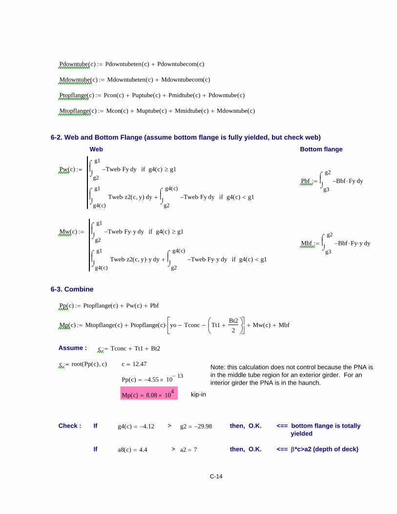
Pdowntube c( ) Pdowntubeten c( ) Pdowntubecom c( )+:=
Mdowntube c( ) Mdowntubeten c( ) Mdowntubecom c( )+:=
Ptopflange c( ) Pcon c( ) Puptube c( )+ Pmidtube c( )+ Pdowntube c( )+:=
Mtopflange c( ) Mcon c( ) Muptube c( )+ Mmidtube c( )+ Mdowntube c( )+:=
6-2. Web and Bottom Flange (assume bottom flange is fully yielded, but check web) Web Bottom flange
Pw c( )g2
g1yTweb− Fy⋅
⌠⎮⌡
d g4 c( ) g1≥if
g4 c( )
g1yTweb z2 c y, ( )⋅
⌠⎮⌡
dg2
g4 c( )yTweb− Fy⋅
⌠⎮⌡
d+ g4 c( ) g1<if
:=
Pbfg3
g2yBbf− Fy⋅
⌠⎮⌡
d:=
Mw c( )g2
g1yTweb− Fy⋅ y⋅
⌠⎮⌡
d g4 c( ) g1≥if
g4 c( )
g1yTweb z2 c y, ( )⋅ y⋅
⌠⎮⌡
dg2
g4 c( )yTweb− Fy⋅ y⋅
⌠⎮⌡
d+ g4 c( ) g1<if
:=
Mbfg3
g2yBbf− Fy⋅ y⋅
⌠⎮⌡
d:=
6-3. Combine
Pp c( ) Ptopflange c( ) Pw c( )+ Pbf+:=
Mp c( ) Mtopflange c( ) Ptopflange c( ) yo Tconc− Tt1Bt22
+⎛⎜⎝
⎞⎟⎠
−⎡⎢⎣
⎤⎥⎦
⋅+ Mw c( )+ Mbf+:=
Assume : c Tconc Tt1+ Bt2+:=
c root Pp c( ) c, ( ):= c 12.47= Note: this calculation does not control because the PNA isin the middle tube region for an exterior girder. For aninterior girder the PNA is in the haunch.Pp c( ) 4.55− 10 13−
×=
Mp c( ) 8.08 104×= kip-in
Check : If g4 c( ) 4.12−= > g2 29.98−= then, O.K. <== bottom flange is totally yielded
If a8 c( ) 4.4= > a2 7= then, O.K. <== β*c>a2 (depth of deck)
C-14

If Tconc Tt1+ Bt2+ 18.63= < c 12.47= < Tconc 2 Tt1⋅+ Bt2+ 19= then, O.K.
<== PNA is in the bottom of the steel tube. Otherwise ignore the above calculations.
Dweb_comp c Tconc− 2 Tt1⋅ Bt2+( )−:=
Dweb_cp Dweb_comp Dweb_comp 0>if
0 otherwise
:=
Dweb_cp 0= in Depth of web in compression
---------------------------------------------------------------------------------------------------------------------------------------------------------------
7. Assume PNA is in WebDeck and concrete in tube(assumes β*c>a2, check later)7-1. Rectangular CFT Compression Flange and Deck
Pcon c( )a2
a1y0.85 fc⋅ Beff⋅
⌠⎮⌡
da8 c( )
a4y0.85 fc⋅ Bt1 2 Tt2⋅−( )⋅
⌠⎮⌡
d+ a8 c( ) a5≥if
a2
a1y0.85 fc⋅ Beff⋅
⌠⎮⌡
da5
a4y0.85 fc⋅ Bt1 2 Tt2⋅−( )⋅
⌠⎮⌡
d+ a8 c( ) a5<if
:=
Mcon c( )a2
a1y0.85 fc⋅ Beff⋅ y⋅
⌠⎮⌡
da8 c( )
a4y0.85 fc⋅ Bt1 2 Tt2⋅−( )⋅ y⋅
⌠⎮⌡
d+ a8 c( ) a5≥if
a2
a1y0.85 fc⋅ Beff⋅ y⋅
⌠⎮⌡
da5
a4y0.85 fc⋅ Bt1 2 Tt2⋅−( )⋅ y⋅
⌠⎮⌡
d+ a8 c( ) a5<if
:=
Top plate of tubePuptube c( )
a4
a3yBt1 z1 c y, ( )⋅
⌠⎮⌡
d a10 c( ) a3>if
a10 c( )
a3yBt1 Fy⋅
⌠⎮⌡
da4
a10 c( )yBt1 z1 c y, ( )⋅
⌠⎮⌡
d+ a4 a10 c( )< a3≤if
a4
a3yBt1 Fy⋅
⌠⎮⌡
d a10 c( ) a4≤if
:=
Muptube c( )a4
a3yBt1 z1 c y, ( )⋅ y⋅
⌠⎮⌡
d a10 c( ) a3>if
a10 c( )
a3yBt1 Fy⋅ y⋅
⌠⎮⌡
da4
a10 c( )yBt1 z1 c y, ( )⋅ y⋅
⌠⎮⌡
d+ a4 a10 c( )< a3≤if
a4
a3yBt1 Fy⋅ y⋅
⌠⎮⌡
d a10 c( ) a4≤if
:=
C-15
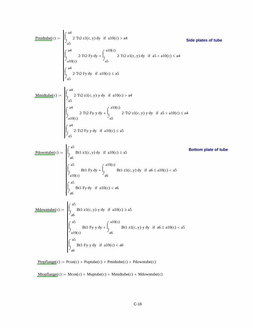
Pmidtube c( )a5
a4y2 Tt2⋅ z1 c y, ( )⋅
⌠⎮⌡
d a10 c( ) a4>if
a10 c( )
a4y2 Tt2⋅ Fy⋅
⌠⎮⌡
da5
a10 c( )y2 Tt2⋅ z1 c y, ( )⋅
⌠⎮⌡
d+ a5 a10 c( )< a4≤if
a5
a4y2 Tt2⋅ Fy⋅
⌠⎮⌡
d a10 c( ) a5≤if
:= Side plates of tube
Mmidtube c( )a5
a4y2 Tt2⋅ z1 c y, ( )⋅ y⋅
⌠⎮⌡
d a10 c( ) a4>if
a10 c( )
a4y2 Tt2⋅ Fy⋅ y⋅
⌠⎮⌡
da5
a10 c( )y2 Tt2⋅ z1 c y, ( )⋅ y⋅
⌠⎮⌡
d+ a5 a10 c( )< a4≤if
a5
a4y2 Tt2⋅ Fy⋅ y⋅
⌠⎮⌡
d a10 c( ) a5≤if
:=
Bottom plate of tubePdowntube c( )
a6
a5yBt1 z1 c y, ( )⋅
⌠⎮⌡
d a10 c( ) a5≥if
a10 c( )
a5yBt1 Fy⋅
⌠⎮⌡
da6
a10 c( )yBt1 z1 c y, ( )⋅
⌠⎮⌡
d+ a6 a10 c( )≤ a5<if
a6
a5yBt1 Fy⋅
⌠⎮⌡
d a10 c( ) a6<if
:=
Mdowntube c( )a6
a5yBt1 z1 c y, ( )⋅ y⋅
⌠⎮⌡
d a10 c( ) a5≥if
a10 c( )
a5yBt1 Fy⋅ y⋅
⌠⎮⌡
da6
a10 c( )yBt1 z1 c y, ( )⋅ y⋅
⌠⎮⌡
d+ a6 a10 c( )≤ a5<if
a6
a5yBt1 Fy⋅ y⋅
⌠⎮⌡
d a10 c( ) a6<if
:=
Ptopflange c( ) Pcon c( ) Puptube c( )+ Pmidtube c( )+ Pdowntube c( )+:=
Mtopflange c( ) Mcon c( ) Muptube c( )+ Mmidtube c( )+ Mdowntube c( )+:=
C-16

7-2. Web and Bottom Flange Parts (assume bottom flange and web may be partially yielded)
Web
Pwten c( )g4 c( )
g6 c( )yTweb z2 c y, ( )⋅
⌠⎮⌡
dg2
g4 c( )yTweb− Fy⋅
⌠⎮⌡
d+ g4 c( ) g2>if
g2
g6 c( )yTweb z2 c y, ( )⋅
⌠⎮⌡
d g4 c( ) g2≤if
:=
Mwten c( )g4 c( )
g6 c( )yTweb z2 c y, ( )⋅ y⋅
⌠⎮⌡
dg2
g4 c( )yTweb− Fy⋅ y⋅
⌠⎮⌡
d+ g4 c( ) g2>if
g2
g6 c( )yTweb z2 c y, ( )⋅ y⋅
⌠⎮⌡
d g4 c( ) g2≤if
:=
Pwcom c( )g6 c( )
g1yTweb z2 c y, ( )⋅
⌠⎮⌡
d g5 c( ) g1>if
g5 c( )
g1yTweb Fy⋅
⌠⎮⌡
dg6 c( )
g5 c( )yTweb z2 c y, ( )⋅
⌠⎮⌡
d+ g5 c( ) g1≤if
:=
Mwcom c( )g6 c( )
g1yTweb z2 c y, ( )⋅ y⋅
⌠⎮⌡
d g5 c( ) g1>if
g5 c( )
g1yTweb Fy⋅ y⋅
⌠⎮⌡
dg6 c( )
g5 c( )yTweb z2 c y, ( )⋅ y⋅
⌠⎮⌡
d+ g5 c( ) g1≤if
:=
Pw c( ) Pwten c( ) Pwcom c( )+:= Mw c( ) Mwten c( ) Mwcom c( )+:=
Bottom flange
Pbf c( )g3
g2yBbf− Fy⋅
⌠⎮⌡
d g4 c( ) g2>if
g4 c( )
g2yBbf z2 c y, ( )⋅
⌠⎮⌡
dg3
g4 c( )yBbf− Fy⋅
⌠⎮⌡
d+ g3 g4 c( )< g2≤if
g3
g2yBbf z2 c y, ( )⋅
⌠⎮⌡
d g4 c( ) g3≤if
:=
C-17
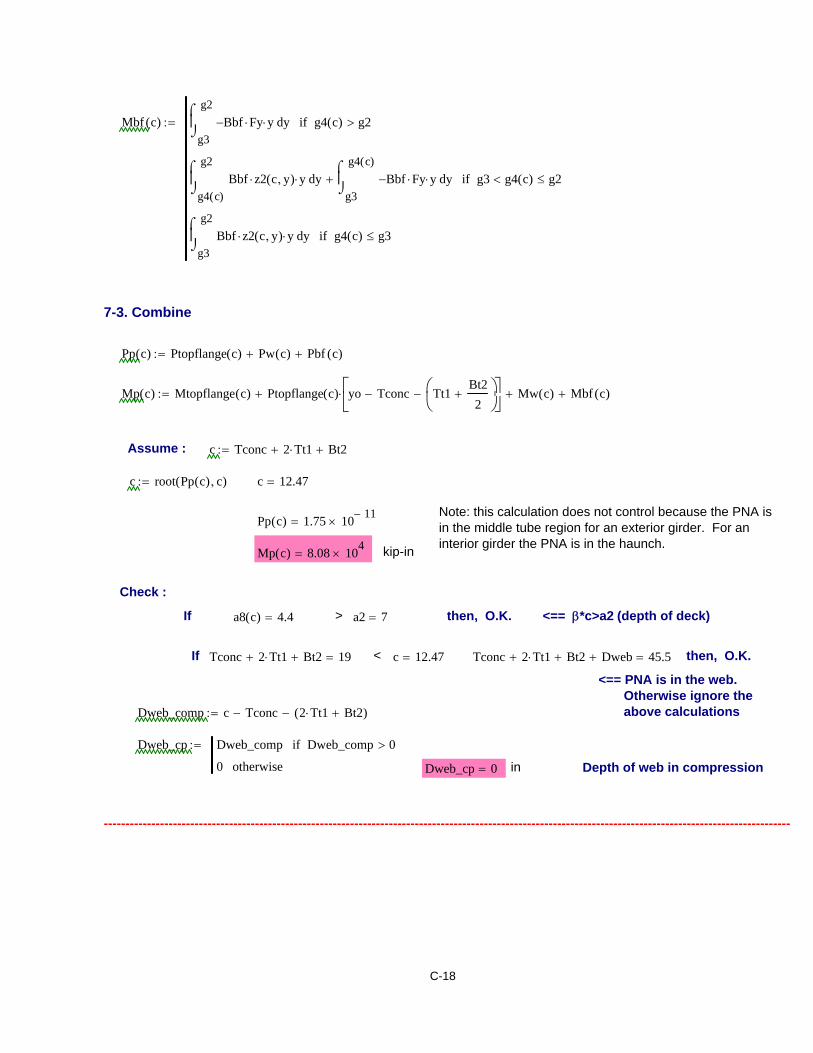
Mbf c( )g3
g2yBbf− Fy⋅ y⋅
⌠⎮⌡
d g4 c( ) g2>if
g4 c( )
g2yBbf z2 c y, ( )⋅ y⋅
⌠⎮⌡
dg3
g4 c( )yBbf− Fy⋅ y⋅
⌠⎮⌡
d+ g3 g4 c( )< g2≤if
g3
g2yBbf z2 c y, ( )⋅ y⋅
⌠⎮⌡
d g4 c( ) g3≤if
:=
7-3. Combine
Pp c( ) Ptopflange c( ) Pw c( )+ Pbf c( )+:=
Mp c( ) Mtopflange c( ) Ptopflange c( ) yo Tconc− Tt1Bt22
+⎛⎜⎝
⎞⎟⎠
−⎡⎢⎣
⎤⎥⎦
⋅+ Mw c( )+ Mbf c( )+:=
Assume : c Tconc 2 Tt1⋅+ Bt2+:=
c root Pp c( ) c, ( ):= c 12.47=
Note: this calculation does not control because the PNA isin the middle tube region for an exterior girder. For aninterior girder the PNA is in the haunch.
Pp c( ) 1.75 10 11−×=
Mp c( ) 8.08 104×= kip-in
Check :
If a8 c( ) 4.4= > a2 7= then, O.K. <== β*c>a2 (depth of deck)
If Tconc 2 Tt1⋅+ Bt2+ 19= < c 12.47= <Tconc 2 Tt1⋅+ Bt2+ Dweb+ 45.5= then, O.K.
<== PNA is in the web. Otherwise ignore the above calculationsDweb_comp c Tconc− 2 Tt1⋅ Bt2+( )−:=
Dweb_cp Dweb_comp Dweb_comp 0>if
0 otherwise
:=
Dweb_cp 0= in Depth of web in compression
---------------------------------------------------------------------------------------------------------------------------------------------------------------
C-18

Appendix D. Yield Moment for Non-composite Section Using Stress Block
1. Conditions and Assumptions- The steel is elastic and the concrete in the tube is represented by the appropriate concrete stressblock.
- c is the location of the elastic neutral axis referenced from the top of the steel tube.
- If c is less than Dgirder/2, then the bottom flange will yield first.
- If c is greater than Dgirder/2, then the steel tube will yield first.
- Compression is positive.
2. Properties and Dimensions (yellow highlight indicates input data)MATERIAL PROPERTIES
Yield Strength (ksi) Young's Modulus (ksi) Concrete Strength (ksi) Modular ratio (input)
Fy 50:= E 29000:= fc 4:= n 8:=
Yield Strain (ksi) Concrete Modulus (ksi) Concrete StressBlock Parameter
Max. Concrete Strain Modular ratio (actual)
εyFyE
:= Ec57000 fc 1000⋅⋅
1000:= β1 0.85:= εucon 0.003:=
EEc
8.0444=
STEEL GIRDER DIMENSIONS
Tube horizontal platethickness
Tube vertical platethickness
Bottom flangethickness
Webthickness
Tt138
:= inches Tt238
:= inches Tbf 1.5:= inches Tweb816
:= inches
Tube horizontal platewidth
Tube vertical platewidth
Bottom flangewidth
Bt1 16:= inches Bt2 7.25:= inches Bbf 18:= inches
Web depth Dweb 36 2 Tt1⋅− Bt2− Tbf−:= Dweb 26.5= inches
Total girder depth Dgirder Tbf Dweb+ 2 Tt1⋅+ Bt2+:= Dgirder 36= inches
NON-COMPOSITE GIRDER PROPERTIES
Abf Bbf Tbf⋅:= Abf 27= in2 Area of bottom flange
Atube 2 Tt1⋅ Bt1⋅ 2 Tt2⋅ Bt2⋅+:= Atube 17.44= in2 Area of tube
Aw Dweb Tweb⋅:= Aw 13.25= in2 Area of web
Asteel Aw Atube+ Abf+:= Asteel 57.69= in2 Total steel area
AconBt2 Bt1 2 Tt2⋅−( )⋅
n:= Acon 13.8203= in2 Equivalent area of concrete in tube (short term)
A Acon Asteel+:= A 71.5= in2 Transformed area of non-composite girder including concrete in tube
D-1
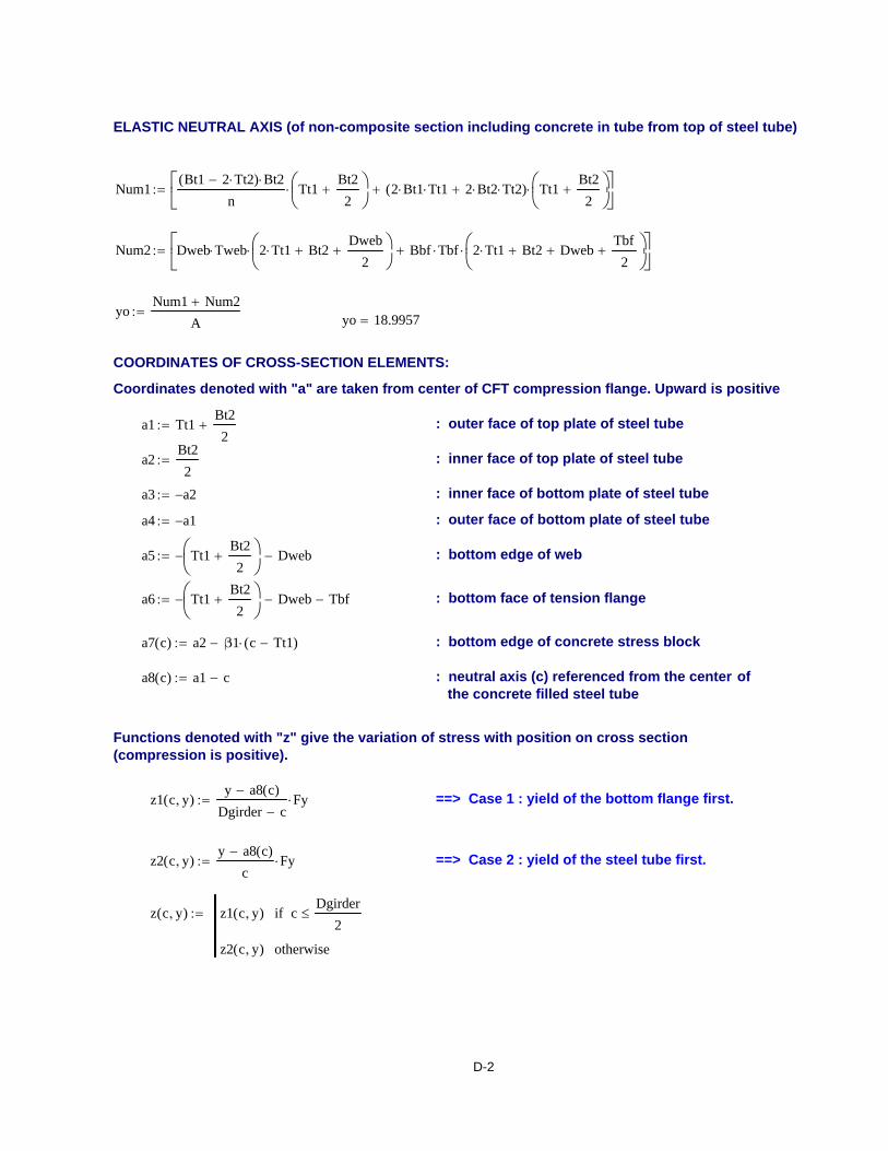
ELASTIC NEUTRAL AXIS (of non-composite section including concrete in tube from top of steel tube)
Num1Bt1 2 Tt2⋅−( ) Bt2⋅
nTt1
Bt22
+⎛⎜⎝
⎞⎟⎠
⋅ 2 Bt1⋅ Tt1⋅ 2 Bt2⋅ Tt2⋅+( ) Tt1Bt22
+⎛⎜⎝
⎞⎟⎠
⋅+⎡⎢⎣
⎤⎥⎦
:=
Num2 Dweb Tweb⋅ 2 Tt1⋅ Bt2+Dweb
2+⎛⎜
⎝⎞⎟⎠
⋅ Bbf Tbf⋅ 2 Tt1⋅ Bt2+ Dweb+Tbf2
+⎛⎜⎝
⎞⎟⎠
⋅+⎡⎢⎣
⎤⎥⎦
:=
yoNum1 Num2+
A:= yo 18.9957=
COORDINATES OF CROSS-SECTION ELEMENTS:
Coordinates denoted with "a" are taken from center of CFT compression flange. Upward is positive
a1 Tt1Bt22
+:= : outer face of top plate of steel tube
a2Bt22
:= : inner face of top plate of steel tube
a3 a2−:= : inner face of bottom plate of steel tube
a4 a1−:= : outer face of bottom plate of steel tube
a5 Tt1Bt22
+⎛⎜⎝
⎞⎟⎠
− Dweb−:= : bottom edge of web
a6 Tt1Bt22
+⎛⎜⎝
⎞⎟⎠
− Dweb− Tbf−:= : bottom face of tension flange
a7 c( ) a2 β1 c Tt1−( )⋅−:= : bottom edge of concrete stress block
a8 c( ) a1 c−:= : neutral axis (c) referenced from the center of the concrete filled steel tube
Functions denoted with "z" give the variation of stress with position on cross section(compression is positive).
z1 c y, ( )y a8 c( )−
Dgirder c−Fy⋅:= ==> Case 1 : yield of the bottom flange first.
z2 c y, ( )y a8 c( )−
cFy⋅:= ==> Case 2 : yield of the steel tube first.
z c y, ( ) z1 c y, ( ) cDgirder
2≤if
z2 c y, ( ) otherwise
:=
D-2

3. Calculation of Yield MomentStress block for concrete in tube
Pc c( )a3
a2y0.85 fc⋅ Bt1 2 Tt2⋅−( )⋅
⌠⎮⌡
d a7 c( ) a3<if
a7 c( )
a2y0.85 fc⋅ Bt1 2 Tt2⋅−( )⋅
⌠⎮⌡
d otherwise
:= Mc c( )a3
a2y0.85 fc⋅ Bt1 2 Tt2⋅−( )⋅ y⋅
⌠⎮⌡
d a7 c( ) a3<if
a7 c( )
a2y0.85 fc⋅ Bt1 2 Tt2⋅−( )⋅ y⋅
⌠⎮⌡
d otherwise
:=
Top plate of steel tube
Put c( )a2
a1yBt1 z c y, ( )⋅
⌠⎮⌡
d:= Mut c( )a2
a1yBt1 z c y, ( )⋅ y⋅
⌠⎮⌡
d:=
Side plates of steel tube
Pmt c( )a3
a2y2 Tt2⋅ z c y, ( )⋅
⌠⎮⌡
d:= Mmt c( )a3
a2y2 Tt2⋅ z c y, ( )⋅ y⋅
⌠⎮⌡
d:=
Bottom plate of steel tube
Pdt c( )a4
a3yBt1 z c y, ( )⋅
⌠⎮⌡
d:= Mdt c( )a4
a3yBt1 z c y, ( )⋅ y⋅
⌠⎮⌡
d:=
Web
Pw c( )a5
a4yTweb z c y, ( )⋅
⌠⎮⌡
d:= Mw c( )a5
a4yTweb z c y, ( )⋅ y⋅
⌠⎮⌡
d:=
Bottom flange
Pbf c( )a6
a5yBbf z c y, ( )⋅
⌠⎮⌡
d:= Mbf c( )a6
a5yBbf z c y, ( )⋅ y⋅
⌠⎮⌡
d:=
Py c( ) Pc c( ) Put c( )+ Pmt c( )+ Pdt c( )+ Pw c( )+ Pbf c( )+:=
My c( ) Mc c( ) Mut c( )+ Mmt c( )+ Mdt c( )+ Mw c( )+ Mbf c( )+:=
Assume : c yo:=
c root Py c( ) c, ( ):= c 19.9839= inPy c( ) 0= (should be zero)
My c( ) 3.5401 104×= kip-in My My c( ):=
My 35401= kip-in
D-3

4. Check Results and Calculate Stresses
If c 19.9839= < Dgirder2
18= then, bottom flange yields first.
Ifc 19.9839= > Dgirder
218= then, steel tube yields first.
fstopatyield z c a1, ( ):= fsbottomatyield z c a6, ( ):=
fstopatyield 50.00= ==> stress of top fiber of steel tube
fsbottomatyield 40.07−= ==> stress of bottom fiber of bottom flange
5. Calculate Stresses due to MDC (unfactored) for Non-Composite Section Using Stress Block
MDC 18720:= kip-in (from Appendix A) My 3.5401 104×= kip-in
"z" gives the variation of stress with position on cross section as function of stress on bottom flange.
z c y, fs, ( )y a8 c( )−
Dgirder c−fs⋅:= ==> Based on absolute value of stress of bottom flange (fs)
Express corresponding forces to determine neutral axis location and bottom flange stress.
Stress block for concrete in tube
Pc c fs, ( )a3
a2y0.85 fc⋅ Bt1 2 Tt2⋅−( )⋅
⌠⎮⌡
d a7 c( ) a3<if
a7 c( )
a2y0.85 fc⋅ Bt1 2 Tt2⋅−( )⋅
⌠⎮⌡
d otherwise
:= Mc c fs, ( )a3
a2y0.85 fc⋅ Bt1 2 Tt2⋅−( )⋅ y⋅
⌠⎮⌡
d a7 c( ) a3<if
a7 c( )
a2y0.85 fc⋅ Bt1 2 Tt2⋅−( )⋅ y⋅
⌠⎮⌡
d otherwise
:=
Top plate of steel tube
Put c fs, ( )a2
a1yBt1 z c y, fs, ( )⋅
⌠⎮⌡
d:= Mut c fs, ( )a2
a1yBt1 z c y, fs, ( )⋅ y⋅
⌠⎮⌡
d:=
Side plates of steel tube
Pmt c fs, ( )a3
a2y2 Tt2⋅ z c y, fs, ( )⋅
⌠⎮⌡
d:= Mmt c fs, ( )a3
a2y2 Tt2⋅ z c y, fs, ( )⋅ y⋅
⌠⎮⌡
d:=
Bottom plate of steel tube
Pdt c fs, ( )a4
a3yBt1 z c y, fs, ( )⋅
⌠⎮⌡
d:= Mdt c fs, ( )a4
a3yBt1 z c y, fs, ( )⋅ y⋅
⌠⎮⌡
d:=
Web
Pw c fs, ( )a5
a4yTweb z c y, fs, ( )⋅
⌠⎮⌡
d:= Mw c fs, ( )a5
a4yTweb z c y, fs, ( )⋅ y⋅
⌠⎮⌡
d:=
Bottom flange
Pbf c fs, ( )a6
a5yBbf z c y, fs, ( )⋅
⌠⎮⌡
d:= Mbf c fs, ( )a6
a5yBbf z c y, fs, ( )⋅ y⋅
⌠⎮⌡
d:=
D-4
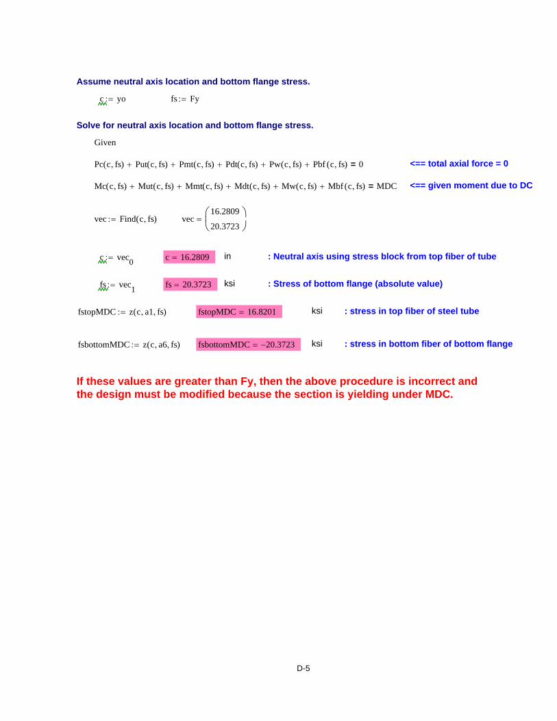
Assume neutral axis location and bottom flange stress.
c yo:= fs Fy:=
Solve for neutral axis location and bottom flange stress.
Given
Pc c fs, ( ) Put c fs, ( )+ Pmt c fs, ( )+ Pdt c fs, ( )+ Pw c fs, ( )+ Pbf c fs, ( )+ 0= <== total axial force = 0
Mc c fs, ( ) Mut c fs, ( )+ Mmt c fs, ( )+ Mdt c fs, ( )+ Mw c fs, ( )+ Mbf c fs, ( )+ MDC= <== given moment due to DC
vec Find c fs, ( ):= vec16.2809
20.3723⎛⎜⎝
⎞⎟⎠
=
c vec0:= c 16.2809= in : Neutral axis using stress block from top fiber of tube
fs vec1:= fs 20.3723= ksi : Stress of bottom flange (absolute value)
fstopMDC z c a1, fs, ( ):= fstopMDC 16.8201= ksi : stress in top fiber of steel tube
fsbottomMDC z c a6, fs, ( ):= fsbottomMDC 20.3723−= ksi : stress in bottom fiber of bottom flange
If these values are greater than Fy, then the above procedure is incorrect andthe design must be modified because the section is yielding under MDC.
D-5
Related Documents