Study of transient heat conduction in 2.5D domains using ...€¦ · Keywords: Transient heat conduction; Cylinder; Fourier transform; 2.5D problem 1. Introduction Carslaw and Jaeger’s

Study of transient heat conduction in 2.5D domains

using the boundary element method

Luıs Godinho*, Antonio Tadeu, Nuno Simoes

Department of Civil Engineering, University of Coimbra, Polo II-Pinhal de Marrocos, Coimbra 3030-290, Portugal

Received 14 April 2003; revised 29 September 2003; accepted 30 September 2003

Abstract

This paper presents the solution for transient heat conduction around a cylindrical irregular inclusion of infinite length, inserted in a

homogeneous elastic medium and subjected to heat point sources placed at some point in the host medium. The solution is computed in the

frequency domain for a wide range of frequencies and axial wavenumbers, and time series are then obtained by means of (fast) inverse

Fourier transforms into space–time.

The method and the expressions presented are implemented and validated by applying them to a cylindrical circular inclusion placed in an

infinite homogeneous medium and subjected to a point heat source, for which the solution is calculated in closed form.

The boundary elements method is then used to evaluate the temperature field generated by a point source in the presence of a cylindrical

inclusion, with a non-circular cross-section, inserted in an unbounded homogeneous medium. Simulation analyses using this model are then

performed to study the transient heat conduction in the vicinity of these inclusions.

q 2003 Elsevier Ltd. All rights reserved.

Keywords: Transient heat conduction; Cylinder; Fourier transform; 2.5D problem

1. Introduction

Carslaw and Jaeger’s book [1] is a reference work on

heat transfer, containing analytical solutions and Green’s

functions for the diffusion equation. In the same work, an

extensive survey of numerical methods applicable in the

study of this phenomenon is also presented. These are

usually grouped by the manner they deal with the time-

dependent terms. One of these is a ‘time marching’

approach, with the solution being evaluated step by step,

at successive time intervals, starting from a specified initial

state of the system. Another approach makes use of the

Laplace transform of the time domain diffusion equation,

which becomes elliptical. A numerical transform inversion

can be used to calculate the physical variables in the time

domain, after the solution being obtained for a sequence of

values of the transform parameter.

A variety of numerical techniques have been proposed to

model and analyze the heat transfer, such as the finite

elements [2], the finite differences [3] and the boundary

elements method [4]. Among these techniques, the Bound-

ary Element Method (BEM) is possibly the method best

suited to analyze infinite or semi-infinite domains, since it

automatically satisfies the far field conditions and only

requires a discretization of the interior boundaries of the

problem, while the finite elements and the finite differences

methods require the full discretization of the domain being

studied, which entails highly expensive numerical compu-

tational schemes.

The BEM allows a compact description of the region,

discretizing only the material discontinuities. Although,

the BEM leads to a fully populated system of equations,

as opposed to the sparse system given by the finite

difference and finite element schemes. The technique is

efficient because it substantially reduces the size of the

system of equations that needs to be solved. It is well

known that the BEM uses the appropriate fundamental

solutions, or Green’s functions, to relate the field variables

in a homogeneous medium to point sources placed within

it. The fundamental solution most often used is that for an

infinite homogeneous space, because it is known in closed

form and has a relatively simple structure. One of the

drawbacks of the BEM is that it can only be applied to

0955-7997/$ - see front matter q 2003 Elsevier Ltd. All rights reserved.

doi:10.1016/j.enganabound.2003.09.002

Engineering Analysis with Boundary Elements 28 (2004) 593–606

www.elsevier.com/locate/enganabound

* Corresponding author.

E-mail address: [email protected] (L. Godinho).

http://www.elsevier.com/locate/enganabound

more general geometry and media when the fundamental

solution is known, to avoid the discretization of the

boundary interfaces, and this may not be possible.

In the ‘time marching’ approach, the BEM is used to

obtain the solution at each time step directly in the time

domain. The first time domain direct boundary integral

method was proposed by Chang et al. [5] to study planar

transient heat conduction. Shaw [6] employed also a time-

dependent fundamental solution for studying three-dimen-

sional (3D) bodies. Later, Wrobel and Brebbia [7]

implemented the BEM for axisymmetric diffusion pro-

blems. Dargush and Banerjee [8] also presented a BEM

approach in the time domain, where planar, 3D and

axisymmetric analyses are all addressed with a time domain

convolution.

The dual reciprocity method is another approach, which

takes the time derivative in the diffusion equation as a body

force and employs the time-independent fundamental

solution to Laplace’s equation to generate a boundary

integral equation [9]. This boundary integral equation can

then be solved using a time and space discretization.

Different time-marching schemes can be used, based on the

way the values of temperature and flux up to actual instant

time are computed when solving for a new time step

[10–13].

A drawback of the ‘time marching’ schemes is that they

can lead to unstable solutions. An option is to transform the

time in a transform variable. The first boundary integral

representation for the transient heat conduction analysis,

based on the Laplace transform, has been proposed by Rizzo

and Shippy [14]. Their numerical approach used a Laplace

transform to produce time-independent boundary inte-

gration in the transform domain. Since then, different

authors presented different solutions for the diffusion type

problem using Laplace transforms such as those presented

by Cheng et al. [15] and Zhu et al. [16,17]. Recently,

Sutradhar et al. [18] used a Laplace transform BEM

approach to solve the 3D transient heat conduction in

functionally graded materials, with thermal conductivity

and heat capacitance varying exponentially in one

coordinate.

A major drawback of using Laplace transforms is the

accuracy loss in the inversion process, which magnifies

small truncation errors. Different researchers have

addressed this problem over the years, and a stable

algorithm has been proposed by Stehfest’s [19].

Most of the previous approaches have used the Laplace

transform to move the solution from the time domain to a

transform domain. In the present work, the time Fourier

Transform is used to compute the transient heat conduction

around cylindrical irregular inclusions of infinite length,

located inside a homogeneous elastic medium and heated by

point sources placed at the host medium. A spatial Fourier

transform in the direction in which the geometry does not

vary (the z-direction) is used to calculate the response,

requiring the solution of a sequence of two-dimensional

(2D) problems with different spatial wavenumbers kz:

Finally, inverse space Fourier transforms are used to

compute the full 3D field.

This solution is known in closed form for inclusions with

simple geometry, such as a circular cylinder, for which the

wave equation is separable. However, if the inclusion has an

irregular cross-section the solution is more difficult to

obtain. This paper presents the solution obtained for

different cylindrical inclusions, buried in a homogeneous

solid medium and subjected to heat point sources placed at

some point in the solid, using boundary elements. The

inclusions can be of three different types: a solid inclusion, a

cavity with prescribed null heat fluxes across its boundary

and a cavity with prescribed null temperature along its

boundary.

The solution at each frequency is expressed in terms of

waves with varying wavenumber kz; which is subsequently

Fourier transformed into the spatial domain. The wave-

number transform in discrete form is obtained by consider-

ing an infinite number of virtual heat point sources equally

spaced along the z-axis and at a sufficient distance from each

other to avoid spatial contamination [20]. Time series are

then obtained by means of (fast) inverse Fourier transforms

into space–time, using complex frequencies to avoid the

aliasing phenomena. In addition, the use of complex

frequencies shifts down the frequency axis, in the complex

plane, in order to remove the singularities on (or near) the

axis and to minimize the influence of the neighboring

fictitious sources.

The method presented is implemented and validated by

applying it to a cylindrical circular inclusions submerged in

an infinite homogenous fluid medium subjected to a point

heat source for which the solution is calculated in closed

form.

The remainder of this paper is organized as follows: the

basic equations of the diffusion problem are first described;

then, the paper indicates the main integrals required to solve

the BEM, including the necessary Green’s functions; a brief

validation of the BEM formulation is presented, using

circular cylindrical inclusions, subjected to steady-state heat

diffusion, for which analytical solutions are known; the

proposed BEM model is then used to simulate the heat

propagation in the vicinity of different buried inclusions.

Frequency and time responses are computed over a grid of

receivers for different spatially sinusoidal harmonic line

heat sources.

2. 3D problem formulation

The transient heat conduction in a homogeneous,

isotropic body is described by the diffusion equation

72T ¼

1

K

›T

›tð1Þ

L. Godinho et al. / Engineering Analysis with Boundary Elements 28 (2004) 593–606594

where

72 ¼›2

›x2þ

›2

›y2þ

›2

›z2

!

t is time, Tðt; x; y; zÞ is temperature, K ¼ k=rc is the thermal

diffusivity, k is the thermal conductivity, r is the density and

c is the specific heat. Making use of a Fourier transform in

the time domain this equation can be written in the

frequency domain as

72 þ

ffiffiffiffiffiffiffi2iv

K

r !2 !Tðv; x; y; zÞ ¼ 0 ð2Þ

where i ¼ffiffiffiffi21

pand v is the frequency.

Assuming that the geometry of the problem remains

constant along one direction ðzÞ; the full 3D solution can be

attained as a summation of simpler 2D solutions. This

procedure requires the application of a Fourier transform

along that direction (Tadeu and Kausel [21]). Each 2D

solution is computed for a different spatial wavenumber kz

~72 þ

ffiffiffiffiffiffiffiffiffiffiffiffiffiffiffiffi2iv

K2 ðkzÞ

2

r !2 !~Tðv; x; y; kzÞ ¼ 0 ð3Þ

with

~72 ¼›2

›x2þ

›2

›y2

!

Applying an inverse Fourier transform along kz; the full 3D

heat field is obtained. Assuming the existence of virtual

sources equally spaced, L; along z; this inverse Fourier

transformation becomes discrete, which allows the solution

to be computed by solving a limited number of 2D problems

Tðv; x; y; zÞ ¼2p

L

XMm¼2M

~Tðv; x; y; kzmÞe2ikzmz ð4Þ

with kzm being the axial wavenumber given by kzm ¼ ð2

p=LÞm: The distance L must be sufficiently large to avoid

spatial contamination from the virtual sources. The authors

have used a similar technique in the analysis of wave

propagation inside seismic prospecting boreholes [22] and

outdoor propagation of sound waves in the presence of

obstacles [23].

3. Boundary element formulation

This section will describe the BEM formulation used to

obtain the3Dheatfield generatedby a heat point source placed

in the vicinity of a cylindrical inclusion with an irregular

shape. Three different types of inclusions will be modeled,

namely a solid inclusion, a cavity with null fluxes and a cavity

with null temperatures prescribed along its boundary.

As explained before, the problem can be solved as a

discrete summation of 2D BEM solutions for different kz

wavenumbers, because the geometry of the problem does

not change along one direction (the z-direction). Then, using

the inverse Fourier transform, the 3D field can be

synthesized. The wavenumber transform is obtained in

discrete form, as explained above, by considering an infinite

number of virtual point sources spaced at equal intervals

along the z-axis and at a sufficient distance from each other

to avoid spatial contamination [24].

Since the literature on the BEM is comprehensive, we do

not give full details of the formulation required for the type

of problem presented here [9]. Only a brief description of

the BEM formulation required to solve each 2D problem is

given.

3.1. Solid inclusion

For frequency domain analysis, the temperature ð ~TÞ at

any point of the spatial domain can be calculated making

use of the Helmoltz equation

72 ~Tðx; y;v; kzÞ þ


K2 ðkzÞ

2

r !2

~Tðx; y;v; kzÞ ¼ 0 ð5Þ

where

72 ¼›2

›x2þ

›2

›y2

!

Considering a homogeneous isotropic solid medium of

infinite extent, containing an inclusion of volume V ;

bounded by a surface S; and subjected to an incident heat

wavefield given by ~Tinc; the boundary integral equations can

be constructed by applying the reciprocity theorem, leading

to

along the exterior domain

c ~TðextÞðx0; y0; kz;vÞ

¼ð

SqðextÞðx; y; nn; kz;vÞG

ðextÞðx; y; x0; y0; kz;vÞds

2ð

SHðextÞðx; y; nn; x0; y0; kz;vÞ ~T

ðextÞðx; y; kz;vÞds

þ ~Tincðx0; y0; kz;vÞ ð6Þ

along the interior domain

c ~TðintÞðx0; y0; kz;vÞ

¼ð

SqðintÞðx; y; nn; kz;vÞG

ðintÞðx; y; x0; y0; kz;vÞds

2ð

SHðintÞðx; y; nn; x0; y0; kz;vÞ ~T

ðintÞðx; y; kz;vÞds ð7Þ

In these equations, superscripts int and ext correspond to the

interior and exterior domain, respectively, nn is the unit

outward normal along the boundary, G and H are,

respectively, the fundamental solutions (Green’s functions)

for the temperature ð ~TÞ and heat flux ðqÞ; at ðx; yÞ due to a

virtual point heat load at ðx0; y0Þ: The factor c is a constant

defined by the shape of the boundary, receiving the value

L. Godinho et al. / Engineering Analysis with Boundary Elements 28 (2004) 593–606 595

1/2 if ðx0; y0Þ [ S and is smooth. If the boundary is

discretized into N straight boundary elements, with one

nodal point in the middle of each element, Eqs. (6) and (7)

take the form,

along the exterior domain

XNl¼1

qðextÞlGðextÞkl 2XNl¼1

~TðextÞlHðextÞkl þ ~Tkinc ¼ ck

~TðextÞk ð8Þ

along the interior domain

XNl¼1

qðintÞlGðintÞkl 2XNl¼1

~TðintÞlHðintÞkl ¼ ck~TðintÞk ð9Þ

with qðextÞk and ~TðextÞk being the nodal heat fluxes and

temperatures at element k in the exterior domain, and qðintÞk

and ~TðintÞk being the nodal heat fluxes and temperatures at

element k in the interior domain

HðextÞkl ¼ð

Cl

HðextÞðxl; yl; nl; xk; yk; kz;vÞdCl

HðintÞkl ¼ð

Cl

HðintÞðxl; yl; nl; xk; yk; kz;vÞdCl

GðextÞkl ¼ð

Cl

GðextÞðxl; yl; xk; yk; kz;vÞdCl

GðintÞkl ¼ð

Cl

GðintÞðxl; yl; xk; yk; kz;vÞdCl

where nl is the unit outward normal for the lth boundary

segment Cl: In Eqs. (8) and (9), HðextÞðxl; yl; nl; xk; yk; kz;vÞ

and GðextÞðxl; yl; xk; yk; kz;vÞ are, respectively, the Green’s

functions for heat fluxes and temperatures components in

the exterior medium of the inclusion, while

HðintÞðxl; yl; nl; xk; yk; kz;vÞ and GðintÞðxl; yl; xk; yk; kz;vÞ are,

respectively, the Green’s functions for heat fluxes and

temperatures components in the interior medium of the

inclusion, at point ðxl; ylÞ; caused by a concentrated heat

load acting at the source point ðxk; ykÞ: The factor ck takes

the value 1/2 when the loaded element coincides with the

element being integrated.

The required two-and-a-half dimensional Green’s func-

tions, for temperature and heat flux in Cartesian co-

ordinates, are those for an unbounded solid medium,

Gðxl; yl; xk; yk; kz;vÞ ¼2i

4kH0


K2 ðkzÞ

2

rr

!ð10Þ

Hðxl; yl; nl; xk; yk; kz;vÞ

¼i

4k


K2 ðkzÞ

2

rH1


K2 ðkzÞ

2

rr

!›r

›nl

in which r ¼ffiffiffiffiffiffiffiffiffiffiffiffiffiffiffiffiffiffiffiffiffiffiffiffiffiffiffiðxl 2 xkÞ

2 þ ðyl 2 ykÞ2

pand where Hnð Þ are

Hankel functions of the second kind and order n: The

thermal diffusivity and the thermal conductivity in these

equations are the ones associated with the exterior and

the interior material of the inclusion when incorporated in

Eqs. (8) and (9), respectively.

The integrations in Eqs. (8) and (9) are evaluated using a

Gaussian quadrature scheme, when they are not performed

along the loaded element. For the loaded element, the

existing singular integrands in the source terms of the

Green’s functions are calculated in closed form [25,26].

The final integral equations are manipulated and

combined so as to impose the continuity of temperatures

and heat fluxes along the boundary of the inclusion, to

establish a system of equations. The solution of this system

of equations gives the nodal temperatures and heat fluxes,

which allow the reflected heat field to be defined.

3.2. Cavity with null fluxes along its boundary

In this case, the boundary conditions prescribe null

normal heat fluxes along the boundary S: Thus, Eq. (6) is

simplified to

c ~TðextÞðx0; y0; kz;vÞ

¼ 2ð

SHðextÞðx; y; nn; x0; y0; kz;vÞ ~T

ðextÞðx; y; kz;vÞds

þ ~Tincðx0; y0; kz;vÞ ð11Þ

The solution of this integral for an arbitrary boundary

surface ðSÞ will require again the discretization of the

boundary into N straight boundary elements, following a

procedure similar to one described above.

3.3. Cavity with null temperatures along its boundary

Null temperatures are now prescribed at the surface of

the cavity, which leads to the equationðS

qðextÞðx; y; nn; kz;vÞGðextÞðx; y; x0; y0; kz;vÞds

þ ~Tincðx0; y0; kz;vÞ ¼ 0 ð12Þ

The solution of this equation is again obtained as described

before.

4. Responses in the time domain

The heat in the spatial–temporal domain is obtained by a

numerical inverse fast Fourier transform in kz and frequency

domain. Complex frequencies with a small imaginary part

of the form vc ¼ v2 ih (with h ¼ 0:7Dv; Dv being the

frequency step) are used to avoid the aliasing phenomena. In

the time domain, this shift is later taken into account by

applying an exponential window of the form eht to the

response.

The temporal variation of the source can be arbitrary.

The application of a time Fourier transformation defines the

frequency domain where the BEM solution is required. So,


the frequency domain may range from 0.0 Hz to very high

frequencies. However, it happens that we may cut-off the

upper frequencies of this domain because the heat responses

decrease very fast as the frequency increases. The frequency

0.0 Hz is the static response that can be obtained by limiting

the frequency to zero. As we are using complex frequencies,

the response can be computed because the argument of the

Hankel in Eqs. (8) and (9) is 2ih; that is different than zero.

As stated before, the Fourier transformations are achieved

by discrete summations over wavenumbers and frequencies,

which is mathematically equivalent to adding periodic

sources at spatial intervals L ¼ 2p=Dkz (in the z-axis) and

temporal intervals T ¼ 2p=Dv; with Dkz being the wave-

number step. The spatial separation L must be sufficiently

large to avoid contamination of the response by the periodic

sources. In other words, the contribution to the response by

the fictitious sources must be guaranteed to occur at times

later than T : This goal can also be aided substantially by

shifting the frequency axis slightly downward, that is, by

using complex frequencies with a small imaginary part ðvc ¼

v2 ihÞ: This technique results in a significant attenuation or

virtual elimination of the periodic sources.

5. BEM validation

The BEM algorithm was implemented and validated by

applying it to a cylindrical circular inclusion, as in Fig. 1,

subjected to a harmonic point heat source applied at point O

ðx0; y0Þ; for which the solution is known in closed form and

described in Appendix A. The incident heat field is given by

the expression

~Tincðx; y; kz;vÞ

¼2iA

4kH0


K2 ðkzÞ

2

r ffiffiffiffiffiffiffiffiffiffiffiffiffiffiffiffiffiffiffiffiffiffiffiffiffiffiðx 2 x0Þ

2 þ ðy 2 y0Þ2

q !ð13Þ

where A (J/m) is the amplitude of the source.

Next, the results are obtained for the three scenarios

studied here. First, the inclusion is assumed to be solid and

bonded to the exterior domain, allowing the continuity of

heat fluxes and temperatures. In a second case, null heat

fluxes are imposed at the interface between the cylindrical

inclusion and the exterior domain. One last situation refers

to a circular cylindrical inclusion with null temperatures

along its boundary. For all cases, the thermal properties of

the host medium are kept constant, with

k1 ¼ 0:72 W m21 8C21, c1 ¼ 780 J Kg21 8C21 and

r1 ¼ 1860 Kg m23. When an elastic inclusion is modeled,

its properties are assumed to be k2 ¼ 0:12 W m21 8C21,

c2 ¼ 1380 J Kg21 8C21 and r2 ¼ 510 Kg m23. The simu-

lated systems are heated by a harmonic line source located

at ðx ¼ 20:7 m; y ¼ 0:0 mÞ: All the calculations are

performed in the frequency range ð0; 128 £ 1028 HzÞ with

a frequency increment of Dv ¼ 1028 Hz; defining the

imaginary part of the frequency to be given by h ¼ 0:7

Dv: The results are computed for two different values of the

parameter kz ðkz ¼ 0:0; 1.0 rad/m). Fig. 2 displays the real

and imaginary parts of the responses, with the analytical

responses being represented by solid lines, and the BEM

solutions by marked points. The circle and the triangle

marks indicate the real and imaginary parts of the BEM

responses, respectively, computed using 100 constant

boundary elements.

All the plots reveal an excellent agreement between the

two solutions presented. Very good results were also

obtained for heat sources and receivers placed at different

positions.

6. Applications

Next we consider the heat field generated by a cylindrical

solid inclusion buried in an unbounded solid medium, with a

rectangular cross-section. At time t ¼ 139 h, a point heat

source at a point O creates a spherical heat pulse that

evolves as plotted in Fig. 3a, propagating away from O with

a power that increases linearly from 0 to 1000.0 W. The

field generated is computed at receivers R1; R2 and R3;

located in three planes equally spaced (3 m) along the z-

direction. The geometry of the plane containing the point

source is shown in Fig. 3b.

The thermal conductivity (k1 ¼ 1:4 W m21 8C21), the

density ðr1 ¼ 2300 Kg m23Þ and the specific heat ðc1 ¼

880:0 J Kg21 8C21Þ of the host medium (concrete) are kept

constant in all the analyses. The material of the inclusion

(steel) has a thermal conductivity ðk2Þ of 63:9 W m21 �

8C21; a density ðr2Þ of 7832 Kg m23 and a specific heat

ðc2Þ of 434.0 J Kg21 8C21. The computations are per-

formed in the frequency range (0, 128 £ 1027 Hz), with a

frequency increment of 1 £ 1027 Hz, which determines

the total time duration ðT ¼ 2778 hÞ for the analysis in the

time domain. The spatial period considered in the analysisFig. 1. Cylindrical circular solid inclusion in an unbounded solid medium.

Medium properties.


is L ¼ 2ffiffiffiffiffiffiffiffiffiffiffiffiffiffik2=ðr2c2Df Þ

p¼ 28 m: The inclusion has been

modeled with 80 boundary elements.

Figs. 4a shows the results obtained at receivers R1; R2

and R3: To allow a better understanding of the physics of the

problem, the results are compared with those computed at

the same receivers for an infinite homogeneous medium,

displayed in Fig. 4b. For all plots, the time response begins

at null temperature, corresponding to the initial conditions

defined for the present problem. As the source starts

emitting energy ðt ¼ 139:0 hÞ; the temperature at the

receivers increases progressively.

The receivers located at z ¼ 0:0 m (Fig. 4a) are the first

to register a clear change in temperature. Of these, receiver

R1; located closest to the heat source, registers the

temperature changes most quickly. The temperature regis-

tered at this point increases smoothly as the energy

generated at the source point increases from 0 to

1000.0 W, reaching approximately 32.0 8C when the source

reaches maximum power ðt < 695:0 hÞ: As the source

stabilizes at 1000.0 W, the temperature continues to

increase at a slower rate, and a maximum value of 39.0 8C

is reached for t < 1250:0 h: At this point, the source power

starts to decline until it stops emitting energy completely.

The energy introduced at the source point continues to

propagate to colder regions in order to establish the

equilibrium condition. Since the analysis is performed for

Fig. 2. Real and imaginary parts of the heat responses: (a) Cylindrical circular solid inclusion in an unbounded solid medium; (b) cylindrical circular cavity with

null fluxes and (c) cylindrical circular cavity with null temperatures.


an infinite medium, this equilibrium would be reached only

for t ¼ 1: Comparing the response at this receiver with that

computed at receiver R2; placed inside the steel inclusion, it

is clear that the latter reaches much lower temperatures, not

only because it is placed further away from the source but

also because it is inside a material with a much higher

diffusivity. In fact, the energy reaching the steel is spread

over the full section of the block, at higher velocity than in

the host medium, allowing a lower but more uniform

increase in the registered temperatures. The presence of this

steel block also influences the response at receiver R3; for

which the temperature rises at almost the same rate as the

temperature of the steel block.

The responses computed for the case of an infinite

medium further confirm the above explanations. Although,

the shape of the temperature curve registered at receiver R1

is similar to the previous case, it reaches a temperature 2.5

times higher than the earlier one. For this case, the energy

propagation is determined only by the physical character-

istics of the host medium (concrete), and it occurs much

more slowly than before. This thermal energy is thus

retained for longer at regions near the source, allowing the

temperature in this region to reach higher values. The same

phenomenon can be observed at receiver R2; which registers

temperatures twice as high as those of the first case. The

opposite behavior is registered at receiver R3; where the

maximum temperatures are lower than those computed in

the presence of the steel block. At this receiver, the presence

of the steel block allows a larger amount of energy to travel

faster to regions behind it. As a consequence, the

temperature at this receiver starts increasing earlier, when

the steel block is present.

Observing the results computed at receivers placed at

z ¼ 3:0 m; when the steel block is present, it can be seen that

the evolution of temperature at all three receivers is very

similar. In fact, the heat propagation occurs mainly through

the most conductive material, which is the steel block. For

this reason, the higher temperatures are registered at

receiver R2; while the temperatures at the two receivers

located in the concrete medium register slightly lower

temperatures. Analyzing the behavior of the same receivers

in an infinite homogeneous medium, it is evident that the

heating curves have a distinct evolution, and the most

influential factor is the distance between the receiver and the

source. It is also clear that the maximum temperatures occur

at later times, since the concrete has a lower diffusivity than

the steel. These conclusions are corroborated by receivers

placed at z ¼ 6:0 m. At this position, in the presence of the

steel inclusion, the heating curves registered at the two

receivers located outside the inclusion, R1 and R3; are

almost coincident and lower than that observed for the

receiver located inside the steel block ðR2Þ:

In Fig. 5, a sequence of snapshots (t ¼ 500; 1500 and

1750 h) displays the temperature field along a transversal

grid of receivers placed at z ¼ 0:0 m and a longitudinal grid

of receivers placed at x ¼ 20:75 m. These figures show the

resulting temperature fields as contour plots.

As the heat propagates away from the source, the energy

spreads out. At time t ¼ 500 h (Fig. 5a) a large amount of

energy generated by the point source has reached the steel

block, travelling faster along the longitudinal direction of

the inclusion than outside. For the same reason, the regions

behind the inclusion, relative to the source, register higher

temperatures along the transversal grid of receivers than the

other regions, which are at the same distance from the

source. As the time progresses, the energy continues to

spread through the full domain of receivers, generating a

progressive temperature increase. For t ¼ 1500 h (Fig. 5b),

this temperature increase is visible at both grids of receivers.

Analyzing the temperature field along the longitudinal grid,

it is possible to confirm that the presence of the steel block

has allowed a large amount of energy to reach receivers at

large distances from the source. In fact, even for points

located at z ¼ 6:0 m, it is possible to observe a distinct rise

in temperature. As the source power drops to 0 W, the

energy continues to propagate through the media, with a

consequent temperature increase for receivers located

further away from the source, and a fall in temperature at

Fig. 3. (a) Temporal evolution of the heat source and (b) geometry of the problem.


receivers located closer to it. This is visible for t ¼ 1750 h

(Fig. 5c), at receivers placed along the longitudinal grid.

Receivers placed further away from the heat source in the z-

direction are still exhibiting a slight temperature increase,

while those placed closer to the source have already suffered

a significant fall in temperature.

Simulations have also been performed for the case of

inclusions with specified boundary conditions of constant

flux or temperature, where the concrete host medium

maintains the material properties previously defined. Fig. 6

presents the results computed at the receivers R1 and R3

when boundary conditions of either null heat flux (Fig. 6a) or

null boundary temperature are ascribed to the boundary of the

inclusion (Fig. 6b). Since the receivers R2 are located inside

the inclusion, they are not used here.

When null heat fluxes are considered for the boundary

of the inclusion and z ¼ 0:0 m, there is a marked

difference between the temperatures registered at R1 and

R3; with R1 reaching very high temperatures (approxi-

mately 145 8C) and R2 registering maximum temperatures

Fig. 4. Heat curves registered at R1; R2 and R3 for different z-coordinates: (a) homogeneous concrete medium with rectangular inclusion and (b) infinite

homogeneous concrete medium.


close to 5 8C. This behavior can be explained by the fact

that, for this case, the inclusion acts as a thermal insulator,

since the null flux conditions ascribed to the boundary

create a thermal energy concentration on the source side

of the inclusion, producing a temperature rise in the

region between the source and the inclusion. In contrast,

very little energy reaches the region behind the inclusion

and the temperature registered there is very low.

Comparing these results with those presented in Fig. 4,

it is possible to observe that the temperatures registered at

receiver R1 are now much higher than in the previous

cases, mainly because of thermal energy concentration

described above. For receivers placed further away, along

the z-direction, the temperatures registered at the two

receivers tend to approximate between them, although

they still diverge relative to those observed in Fig. 4a, for

the case of the steel inclusion. Because of the 3D

character of the problem, the energy concentration

becomes less evident as we advance in z; and the solution

approaches the one registered for an infinite homogeneous

medium, although with temperatures slightly higher at R1

and lower at R2:

Fig. 5. Temperature fields registered at the two grids of receivers: (a) t ¼ 500 h; (b) t ¼ 1500 h and (c) t ¼ 1750 h.


This scenario changes when null temperature con-

ditions are ascribed to the boundary of the inclusion, as

shown in Fig. 6b. As expected, receiver R1 still registers

higher temperatures than R2; but the maximum tempera-

ture registered is now much lower than in the previous

case, since it is located close to a null temperature

surface. As positions further away in z are considered, the

temperature at R1 decreases markedly, reaching maximum

values below 0.158, even when z ¼ 3:0 m. The tempera-

tures registered in R2 are very low, since the receiver is

close to a boundary 08 and it is placed on the opposite

side of the inclusion from the source. These low

temperatures are even more evident when the receiver is

located further away in z:

Fig. 6. Heat curves registered at R1; R3 for different z-coordinates: rectangular cavity with (a) null fluxes and (b) null temperatures.


To better understand the heat propagation phenomenon

around inclusions with null flux or null temperature

boundary conditions, Fig. 7 present a sequence of

snapshots displaying the temperature field along a

longitudinal grid of receivers located in the plane

x ¼ 20:75 m. The temperature fields are again displayed

as contour plots. At time t ¼ 500 h (Fig. 7a), the effect of

the propagating thermal energy is clearly visible over the

grid of receivers, and the results reveal marked differences

between the two cases analysed. It is possible to observe

that much higher temperatures are registered when null

fluxes are prescribed, particularly at receivers placed

further away in z: In fact, for the second case, the null

temperatures prescribed along the surface of the inclusion

do not allow the same temperature rise, particularly at

larger distances along the z-axis and for receivers placed

closer to the inclusion. As time advances, this difference

remains clearly visible, and for t ¼ 1500 h (Fig. 7b) the

shape of the contour lines in the two plots confirms the

different behaviors observed for the two cases. In the first

case, the imposition of null fluxes along the boundary

allows the energy to be retained in the host medium, while

in the second; the boundary with null temperatures

generates fluxes that tend to drain energy from the system.

This effect is noticeable if one observes the rapid

temperature variation in the direction perpendicular to the

boundary as receivers placed closer to the inclusion are

considered, indicating a strong temperature gradient. When

the null fluxes are considered, however, the temperature

variation along the same direction is much smaller, and it is

much more evident at receivers placed along the direction

of the axis of the inclusion. The same behavior can be seen

in Fig. 7c for t ¼ 1750 h, after the source stops emitting

energy. At this later time, it is interesting to note that, in

Fig. 7. Temperature fields registered along a longitudinal grid of receivers located in the plane x ¼ 20:75 m: (a) t ¼ 500 h; (b) t ¼ 1500 h and (c) t ¼ 1750 h.


both cases, the temperature continues to rise, since the

energy is still propagating away from the source point.

Notice that this behavior differs from that found in the

presence of a steel inclusion, which exhibits higher

diffusivity.

7. Conclusions

A discrete integration over wavenumbers and frequen-

cies has been used to compute the 3D heat field generated by

harmonic heat point sources placed in the vicinity of a

cylindrical irregular inclusion in an unbounded solid

medium. The discretization of the wavenumber–frequency

integral transform presented is mathematically equivalent to

a periodic sequence of sources, parallel to the axis of the

cylinder, that are also periodic in time. We have removed

the effects of these periodicities by using complex

frequencies.

The method was implemented and used to show the main

features of the transient heat conduction across media

containing an inclusion. The time responses obtained made

it possible to confirm that the method presented was useful

in the analysis of 3D heat propagation in the presence of a

2D geometry. The results computed for the three situations

analysed (a solid inclusion, an inclusion with null surface

temperature and an inclusion with null normal fluxes along

its surface) have shown marked differences in their behavior

and the temperature field was found to be strongly

dependent on the prescribed boundary conditions.

Appendix A. Analytical solution of the 3D transient heat

transfer through a cylindrical circular solid inclusion

A.1. Solid inclusion

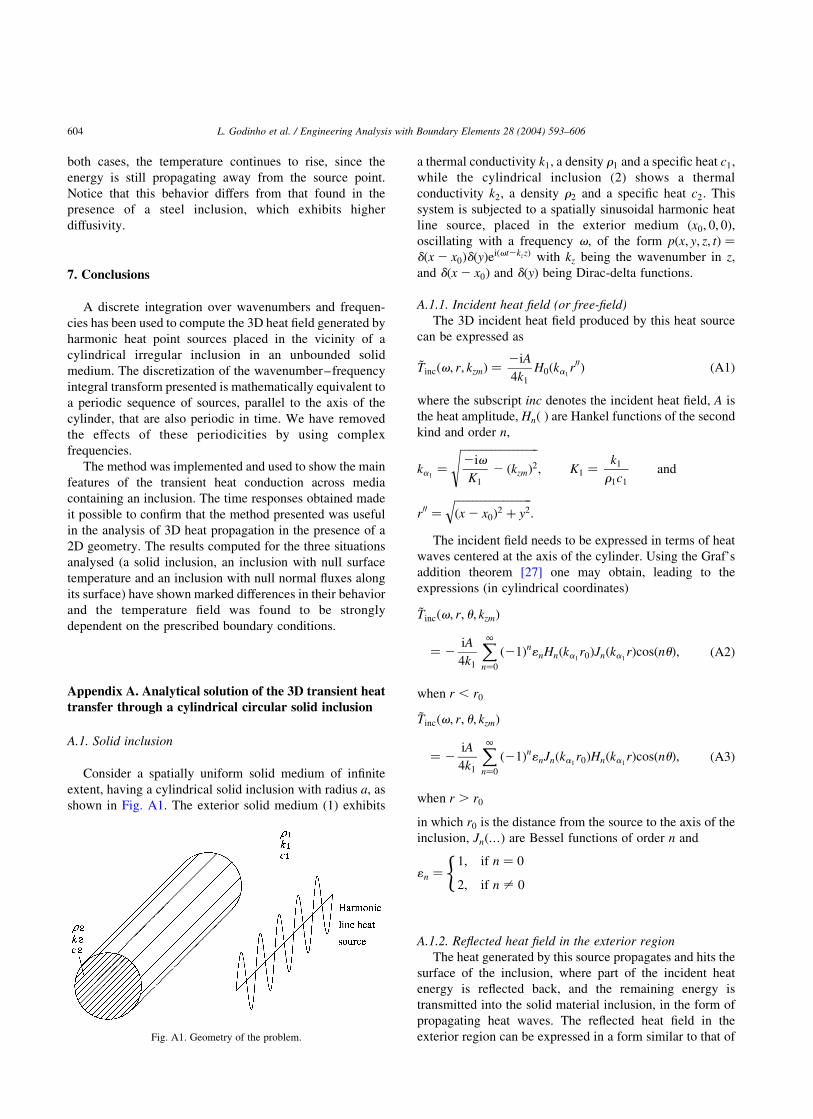
Consider a spatially uniform solid medium of infinite

extent, having a cylindrical solid inclusion with radius a; as

shown in Fig. A1. The exterior solid medium (1) exhibits

a thermal conductivity k1; a density r1 and a specific heat c1;

while the cylindrical inclusion (2) shows a thermal

conductivity k2; a density r2 and a specific heat c2: This

system is subjected to a spatially sinusoidal harmonic heat

line source, placed in the exterior medium ðx0; 0; 0Þ;

oscillating with a frequency v; of the form pðx; y; z; tÞ ¼

dðx 2 x0ÞdðyÞeiðvt2kzzÞ with kz being the wavenumber in z;

and dðx 2 x0Þ and dðyÞ being Dirac-delta functions.

A.1.1. Incident heat field (or free-field)

The 3D incident heat field produced by this heat source

can be expressed as

~Tincðv; r; kzmÞ ¼2iA

4k1

H0ðka1r00Þ ðA1Þ

where the subscript inc denotes the incident heat field, A is

the heat amplitude, Hnð Þ are Hankel functions of the second

kind and order n;

ka1¼

ffiffiffiffiffiffiffiffiffiffiffiffiffiffiffiffiffiffi2iv

K1

2 ðkzmÞ2

s; K1 ¼

k1

r1c1

and

r00 ¼

ffiffiffiffiffiffiffiffiffiffiffiffiffiffiffiffiffiffiðx 2 x0Þ

2 þ y2

q:

The incident field needs to be expressed in terms of heat

waves centered at the axis of the cylinder. Using the Graf’s

addition theorem [27] one may obtain, leading to the

expressions (in cylindrical coordinates)

~Tincðv; r; u; kzmÞ

¼ 2iA

4k1

X1n¼0

ð21Þn1nHnðka1r0ÞJnðka1

rÞcosðnuÞ;

when r , r0

ðA2Þ

~Tincðv; r; u; kzmÞ

¼ 2iA

4k1

X1n¼0

ð21Þn1nJnðka1r0ÞHnðka1

rÞcosðnuÞ;

when r . r0

ðA3Þ

in which r0 is the distance from the source to the axis of the

inclusion, Jnð…Þ are Bessel functions of order n and

1n ¼1; if n ¼ 0

2; if n – 0

(

A.1.2. Reflected heat field in the exterior region

The heat generated by this source propagates and hits the

surface of the inclusion, where part of the incident heat

energy is reflected back, and the remaining energy is

transmitted into the solid material inclusion, in the form of

propagating heat waves. The reflected heat field in the

exterior region can be expressed in a form similar to that ofFig. A1. Geometry of the problem.


the incident field, namely

~Trefðv; r; u; kzmÞ ¼X1n¼0

AnHnðka1rÞcosðnuÞ ðA4Þ

in which the subscript ref denotes the reflected heat field, An

is as yet unknown coefficient to be determined from

appropriate boundary conditions. Together with an implicit

factor eiðvt2kzzÞ; the Hankel functions in Eqs. (A4) represent

diverging or outgoing cylindrical heat waves.

A.1.3. Transmitted heat field in the interior region

The transmitted heat field can be seen as standing heat

waves, which can be expressed as

~Ttransðv; r; u; kzmÞ ¼X1n¼0

BnJnðka2rÞcosðnuÞ ðA5Þ

in which the subscript trans denotes the reflected heat field

ka2¼

ffiffiffiffiffiffiffiffiffiffiffiffiffiffiffiffiffiffi2iv

K2

2 ðkzmÞ2

s; K2 ¼

k2

r2c2

Bn is again an unknown coefficient to be determined by

imposing the appropriate boundary conditions.

A.1.4. Definition of An and Bn

The definition of the appropriate boundary conditions

allows An and Bn; that is the reflected and transmitted heat

field, to be defined. The solution in this case is computed

imposing the continuity of temperatures and normal heat

fluxes on the solid–solid interface

~Tincðv; a; u; kzmÞ þ ~Trefðv; a; u; kzmÞ ¼ ~Ttransðv; a; u; kzmÞ

ðA6Þ

k1

›½ ~Tincðv; a; u; kzmÞ

›rþ k1

›½ ~Trefðv; a; u; kzmÞ

›r

¼ k2

›½ ~Ttransðv; a; u; kzmÞ

›r

Combining Eqs. (A2), (A4) and (A5) one obtains a system

of equations, which is then used to find the coefficients An

and Bn:

A.2. Cavity with null fluxes along its boundary

In this case, the incident heat field is all reflected back

into the unbounded medium after reaching the inclusion

surface, verifying the condition at r ¼ a;

k1

›½ ~Tincðv; a; u; kzmÞ

›rþ k1

›½ ~Trefðv; a; u; kzmÞ

›r¼ 0 ðA7Þ

Under this condition the transmitted heat field is null.

Therefore, the solution is found combining Eqs. (A2) and

(A4), so as to satisfy Eq. (A7). When this is done, one

obtains

An¼

2i

4k1

ð21Þn1nHnðka1r0Þ½2nJnðka1

aÞþðka1aÞJnþ1ðka1

aÞ

nHnðka1aÞ2ðka1

aÞHnþ1ðka1aÞ

ðA8Þ

A.3. Cavity with null temperatures along its boundary

The boundary condition at the surface of the cavity ðr ¼

aÞ is

~Tincðv; a; u; kzmÞ þ ~Trefðv; a; u; kzmÞ ¼ 0 ðA9Þ

Manipulating Eqs. (A2), (A4) and (A9), the following result

is obtained

An ¼

i

4k1

ð21Þn1nHnðka1r0ÞJnðka1

aÞ

Hnðka1aÞ

ðA10Þ

References

[1] Carslaw HS, Jaeger JC. Conduction of heat in solids, 2nd ed. Oxford:

Oxford University Press; 1959.

[2] Bathe KJ. Numerical methods in finite element analysis. Englewood

Cliffs, NJ: Prentice-Hall; 1976.

[3] Freitas V, Abrantes V, Crausse P. Moisture migration in building

walls, analysis of the interface phenomena. Bldg Environ 1996;31(2):

99–108.

[4] Brebbia CA, Telles JC, Wrobel LC. Boundary elements techniques:

theory and applications in engineering. Berlin: Springer; 1984.

[5] Chang YP, Kang CS, Chen DJ. The use of fundamental green

functions for solution of problems of heat conduction in anisotropic

media. Int J Heat Mass Transfer 1973;16:1905–18.

[6] Shaw RP. An integral equation approach to diffusion. Int J Heat Mass

Transfer 1974;17:693–9.

[7] Wrobel LC, Brebbia CA. A formulation of the boundary element

method for axisymmetric transient heat conduction. Int J Heat Mass

Transfer 1981;24:843–50.

[8] Dargush GF, Banerjee PK. Application of the boundary element

method to transient heat conduction. Int J Numer Meth Engng 1991;

31:1231–47.

[9] Wrobel LC. The boundary element method: application in thermo-

fluids and acoustics. Sussex: Wiley; 2001.

[10] Davey K, Bounds S. Source-weighted domain integral approximation

for linear transient heat conduction. Int J Numer Meth Engng 1996;39:

1775–90.

[11] Ibanez MT, Power H. An efficient direct BEM numerical scheme for

heat transfer problems using Fourier series. Int J Numer Meth Heat

Fluid Flow 2000;10:687–720.

[12] Davey K, Bounds S. Source-weighted domain integral approximation

for linear transient heat conduction. Int J Numer Meth Engng 1996;39:

1775–90.

[13] Bialecki RA, Jurgas P, Kuhn G. Dual reciprocity BEM without matrix

inversion for transient heat conduction. Engng Anal Bound Elem

2002;26(3):227–36.

[14] Rizzo FJ, Shippy DJ. A method of solution for certain problems of

transient heat conduction. AIAA J 1970;8:2004–9.


[15] Cheng AHD, Abousleiman Y, Badmus T. A Laplace transform BEM

for axysymmetric diffusion utilizing pre-tabulated Green’s function.

Engng Anal Bound Elem 1992;9:39–46.

[16] Zhu SP, Satravaha P, Lu X. Solving the linear diffusion equations with

the dual reciprocity methods in Laplace space. Engng Anal Bound

Elem 1994;13:1–10.

[17] Zhu SP, Satravaha P. An efficient computational method for nonlinear

transient heat conduction problems. Appl Math Model 1996;20:513–22.

[18] Sutradhar A, Paulino GH, Gray LJ. Transient heat conduction in

homogeneous and non-homogeneous materials by the Laplace

transform Galerkin boundary element method. Engng Anal Bound

Elem 2002;26(2):119–32.

[19] Stehfest H. Algorithm 368: numerical inversion of Laplace transform.

Commun Assoc Comput Mach 1970;13(1):47–9.

[20] Tadeu A, Godinho L. 3D wave scattering by a fixed cylindrical

inclusion submerged in a fluid medium. Engng Anal Bound Elem

1999;23:745–56.

[21] Tadeu A, Kausel E. Green’s functions for two-and-a-half dimensional

elastodynamic problems. J Engng Mech, ASCE 2000;126(10):1093–7.

[22] Tadeu A, Godinho L, Santos P. Wave motion between two fluid filled

boreholes in an elastic medium. Engng Anal Bound Elem 2002;26(2):

101–17.

[23] Godinho L, Antonio J, Tadeu A. 3D sound scattering by rigid

barriers in the vicinity of tall buildings. Appl Acoust 2001;62(11):

1229–48.

[24] Bouchon M, Aki K. Time-domain transient elastodynamic analysis

of 3D solids by BEM. Int J Numer Meth Engng 1977;26:

1709–28.

[25] Tadeu A, Santos P, Kausel E. Closed-form integration of singular

terms for constant, linear and quadratic boundary elements. Part

I. SH wave propagation. Engng Anal Bound Elem 1999;23(8):

671–81.

[26] Tadeu A, Santos P, Kausel E. Closed-form integration of singular

terms for constant, linear and quadratic boundary elements. Part II.

SV-P wave propagation. Engng Anal Bound Elem 1999;23(9):

757–68.

[27] Watson GN. A treatise on the theory of Bessel functions, 2nd ed.

Cambridge: Cambridge University Press; 1980.


Study of transient heat conduction in 2.5D domains using ...€¦ · Keywords: Transient heat conduction; Cylinder; Fourier transform; 2.5D problem 1. Introduction Carslaw and Jaeger’s

Documents