Study of the dynamic behavior of Pelton turbines by Mònica Egusquiza Montagut ADVERTIMENT La consulta d’aquesta tesi queda condicionada a l’acceptació de les següents condicions d'ús: La difusió d’aquesta tesi per mitjà del r e p o s i t o r i i n s t i t u c i o n a l UPCommons (http://upcommons.upc.edu/tesis) i el repositori cooperatiu TDX ( h t t p : / / w w w . t d x . c a t / ) ha estat autoritzada pels titulars dels drets de propietat intel·lectual únicament per a usos privats emmarcats en activitats d’investigació i docència. No s’autoritza la seva reproducció amb finalitats de lucre ni la seva difusió i posada a disposició des d’un lloc aliè al servei UPCommons o TDX. No s’autoritza la presentació del seu contingut en una finestra o marc aliè a UPCommons (framing). Aquesta reserva de drets afecta tant al resum de presentació de la tesi com als seus continguts. En la utilització o cita de parts de la tesi és obligat indicar el nom de la persona autora. ADVERTENCIA La consulta de esta tesis queda condicionada a la aceptación de las siguientes condiciones de uso: La difusión de esta tesis por medio del repositorio institucional UPCommons (http://upcommons.upc.edu/tesis) y el repositorio cooperativo TDR (http://www.tdx.cat/?locale- attribute=es) ha sido autorizada por los titulares de los derechos de propiedad intelectual únicamente para usos privados enmarcados en actividades de investigación y docencia. No se autoriza su reproducción con finalidades de lucro ni su difusión y puesta a disposición desde un sitio ajeno al servicio UPCommons No se autoriza la presentación de su contenido en una ventana o marco ajeno a UPCommons (framing). Esta reserva de derechos afecta tanto al resumen de presentación de la tesis como a sus contenidos. En la utilización o cita de partes de la tesis es obligado indicar el nombre de la persona autora. WARNING On having consulted this thesis you’re accepting the following use conditions: Spreading this thesis by the i n s t i t u t i o n a l r e p o s i t o r y UPCommons (http://upcommons.upc.edu/tesis) and the cooperative repository TDX (http://www.tdx.cat/?locale- attribute=en) has been authorized by the titular of the intellectual property rights only for private uses placed in investigation and teaching activities. Reproduction with lucrative aims is not authorized neither its spreading nor availability from a site foreign to the UPCommons service. Introducing its content in a window or frame foreign to the UPCommons service is not authorized (framing). These rights affect to the presentation summary of the thesis as well as to its contents. In the using or citation of parts of the thesis it’s obliged to indicate the name of the author.

Welcome message from author
This document is posted to help you gain knowledge. Please leave a comment to let me know what you think about it! Share it to your friends and learn new things together.
Transcript

Study of the dynamic behavior of Pelton turbines
by
Mònica Egusquiza Montagut
ADVERTIMENT La consulta d’aquesta tesi queda condicionada a l’acceptació de les següents condicions d'ús: La difusió d’aquesta tesi per mitjà del r e p o s i t o r i i n s t i t u c i o n a l UPCommons (http://upcommons.upc.edu/tesis) i el repositori cooperatiu TDX ( h t t p : / / w w w . t d x . c a t / ) ha estat autoritzada pels titulars dels drets de propietat intel·lectual únicament per a usos privats emmarcats en activitats d’investigació i docència. No s’autoritza la seva reproducció amb finalitats de lucre ni la seva difusió i posada a disposició des d’un lloc aliè al servei UPCommons o TDX. No s’autoritza la presentació del seu contingut en una finestra o marc aliè a UPCommons (framing). Aquesta reserva de drets afecta tant al resum de presentació de la tesi com als seus continguts. En la utilització o cita de parts de la tesi és obligat indicar el nom de la persona autora.
ADVERTENCIA La consulta de esta tesis queda condicionada a la aceptación de las siguientes condiciones de uso: La difusión de esta tesis por medio del repositorio institucional UPCommons (http://upcommons.upc.edu/tesis) y el repositorio cooperativo TDR (http://www.tdx.cat/?locale- attribute=es) ha sido autorizada por los titulares de los derechos de propiedad intelectual únicamente para usos privados enmarcados en actividades de investigación y docencia. No se autoriza su reproducción con finalidades de lucro ni su difusión y puesta a disposición desde un sitio ajeno al servicio UPCommons No se autoriza la presentación de su contenido en una ventana o marco ajeno a UPCommons (framing). Esta reserva de derechos afecta tanto al resumen de presentación de la tesis como a sus contenidos. En la utilización o cita de partes de la tesis es obligado indicar el nombre de la persona autora.
WARNING On having consulted this thesis you’re accepting the following use conditions: Spreading this thesis by the i n s t i t u t i o n a l r e p o s i t o r y UPCommons (http://upcommons.upc.edu/tesis) and the cooperative repository TDX (http://www.tdx.cat/?locale- attribute=en) has been authorized by the titular of the intellectual property rights only for private uses placed in investigation and teaching activities. Reproduction with lucrative aims is not authorized neither its spreading nor availability from a site foreign to the UPCommons service. Introducing its content in a window or frame foreign to the UPCommons service is not authorized (framing). These rights affect to the presentation summary of the thesis as well as to its contents. In the using or citation of parts of the thesis it’s obliged to indicate the name of the author.

Study of the dynamic behavior of Pelton turbines
Doctoral thesis
December 2019
Barcelona
Submitted by
Mònica Egusquiza Montagut
Universitat Politècnica de Catalunya
Dept. of Fluid Mechanics
Doctorate program in Mechanical and Aeronautical Engineering
Thesis Supervisor
Prof. Eduard Egusquiza Estevez


Acknowledgements
I would like to start these acknowledgements by expressing my most sincere gratitude
towards my thesis supervisor and father, Prof. Eduard Egusquiza, and towards my mother,
Carme Montagut, for their unconditional support. Their advice and encouragement over the
course of this thesis, inside and outside the technical field, have made it possible for me to
reach this end.
Next, I would like to acknowledge the assistance provided by my colleagues Dr. Eng. David
Valentín, Dr. Eng. Carme Valero and Dr. Eng. Alex Presas. Thank you very much for sharing
your knowledge and experience with me, especially at the beginning. I really appreciate your
support and I wish we can keep on sharing many good moments together. My thanks to David
Castañer, Paloma Ferrer, Dr. Eng. Alfredo Guardo and the rest of members of the CDIF, who
have also contributed to an enjoyable stay. I would also like to acknowledge the support
received from Prof. Jesús Álvarez during the last stage of the thesis.
Needless to mention the good experiences shared with the doctoral students Eng. Zhao
Weiqiang, Eng. Geng Linlin, Eng. Chen Jian and Dr. Eng. Zhang Ming. I would like to make
a special mention to my dear friend Dr. Eng. He Lingyan, whose company I cherished the
most in my first doctoral year.
I would also like to show my gratitude and appreciation towards the colleagues of VOITH
Hydro, who gave me their support during my stay in Heidenheim, especially to Eng. Nagore
San José and Eng. Christian Probst. I want to thank them, as well as all the other colleagues,
for making my stay so memorable. Thank you very much to Dr. Eng. Jiri Koutnik for giving
me the opportunity to have this experience and to Eng. Reiner Mack for his time and advice
on Pelton turbines.
Thanks to Prof. François Avellan and the colleagues of the LMH for the short but nice stay
in Lausanne.
Finally, I would like to express my gratitude to Oscar, who has always supported and
encouraged me in the distance. Thanks also to my family and friends, whose understanding
and support I have always appreciated. Special thanks to Dr. Paula Garcia for the time spent
together over so many years and for her always-good advice.


Abstract
The future of hydropower is tied to the rapid increase of new renewable energies, such as
photovoltaic and wind energy. With the growing share of intermittent electricity production,
the operation of hydropower installations must be more flexible in order to guarantee the
balance between supply and demand. As a result, turbines must increase their operating
range and undergo more starts and stops, what leads to a faster deterioration of the turbine
components, especially the runner. In the current scenario, condition monitoring constitutes
an essential procedure to assess the state of the turbines while in operation and can help
preventing major damage.
Pelton turbines are used in locations with high heads and low discharges. The runner is
composed by a disk with several attached buckets, which periodically receive the impact of
high speed water jets. Buckets must thus endure large tangential stresses that can lead to
fatigue problems and, in case the natural modes of the runner are excited, this problem can
be severely aggravated. Therefore, a deep comprehension of the modal behavior and
dynamics of Pelton turbines is required in order to keep track of the runner condition with
monitoring systems.
In this thesis, the dynamic behavior of Pelton turbines during different operating conditions
has been studied in detail and the knowledge acquired has been used to upgrade the present
condition monitoring. The first part of the document comprises the study of the modal
behavior of Pelton turbines. A systematic approach has been followed with such purpose; first
a single bucket has been analyzed, second the runner and then the whole turbine. With the
help of numerical models and experimental tests the natural frequencies and mode shapes
have been identified and classified. The effect of the mechanical design and the boundary
conditions has also been discussed.
The second part of the thesis is focused on determining the transmission of the runner
vibrations to the monitoring locations. It is proved that these can be detected from the
bearings and that the transmission depends on the mode type.
In the third and last part the analysis of Pelton turbines in operation is carried out. Two
different machines have been studied during start-up and under different load conditions to
determine which modes are excited, how the frequencies change in operation with respect to
the still machine and how they are detected from different positions. The spectrum frequency
bands corresponding to the runner modes and the overall vibration levels have been
analyzed. Finally, the information obtained has been used to propose an upgrade of the
current practice in condition monitoring. A case of damage has been analyzed with a
numerical model and with historic data to illustrate the strategy.


Resum
El futur de l’energia hidràulica està lligat al ràpid creixement de les noves energies
renovables, tals com l’energia fotovoltaica i l’eòlica. A mesura que la porció d’energia
intermitent que es produeix creix, el funcionament de les instal·lacions hidroelèctriques es
veu forçat a ser més flexible per tal de garantir el balanç entre el subministrament i la
demanda d’energia. Això es tradueix en un increment del rang de funcionament de les
turbines i en més parades i arrancades, fet que contribueix a un deteriorament més ràpid
dels seus components, especialment del rodet. En la situació actual, la monitorització de
l’estat de les turbines és essencial per tal d’assegurar-ne les bones condicions de
funcionament i evitar danys majors.
Les turbines Pelton s’utilitzen en emplaçaments amb salts elevats i cabals reduïts. El rodet
està compost per un disc amb diverses culleres que reben periòdicament l’impacte de raigs
d’aigua a molta velocitat. Com a conseqüència, les culleres han de suportar grans tensions en
direcció tangencial, les quals comporten seriosos problemes de fatiga a l’estructura. En cas
que els modes naturals del rodet també s’excitin pels rajos d’aigua, aquest problema és
altament agreujat. Així, és necessari tenir un coneixement profund del comportament modal
i dinàmic de les turbines Pelton per tal de controlar l’estat del rodet amb sistemes de
monitorització.
En aquesta tesi s’ha estudiat en detall el comportament dinàmic de turbines Pelton en
diferents condicions d’operació. El coneixement adquirit s’ha utilitzat per a millorar el
sistema de monitorització actual. La primera part del document comprèn l’estudi del
comportament modal de turbines Pelton. Amb tal propòsit s’ha abordat el problema de
manera sistemàtica: primer s’han analitzat els modes d’una sola cullera, després els del rodet
sencer i per últim els de tota la turbina. Amb l’ajuda de models numèrics i de proves
experimentals s’han identificat i classificat les corresponents freqüències naturals i formes
modals. A més a més s’ha estudiat l’efecte del disseny mecànic i de les condicions de contorn.
La segona part d’aquesta tesi està centrada en determinar la transmissió de les vibracions
del rodet a les posicions de monitorització. S’ha demostrat que aquestes es poden detectar des
dels coixinets i que la qualitat de la transmissió depèn del tipus de mode.
A la tercera i última part s’ha dut a terme l’anàlisi de turbines Pelton en funcionament. S’han
estudiat dues màquines diferents durant el transitori de posta en marxa i sota diferents
càrregues per tal de determinar quines modes s’exciten, com canvien les freqüències de la
turbina en funcionament respecte la màquina parada i com es detecten des de les diferents
posicions. Les bandes de freqüència de l’espectre de vibració corresponents als diferents
modes del rodet i els nivells de vibració s’han analitzat. Finalment, la informació obtinguda
ha estat utilitzada per a fer una proposta de millora de l’actual procediment de

monitorització. Un cas de dany en un rodet ha estat analitzat amb un model numèric i amb
l’històric de vibracions per tal d’il·lustrar l’estratègia a seguir en un futur.
Resumen
El futuro de la energía hidráulica está relacionado con el rápido crecimiento de las nuevas
energías renovables, tales como la energía fotovoltaica y la eólica. A medida que la porción
de energía intermitente que se produce crece, el funcionamiento de las instalaciones
hidroeléctricas se ve obligado a ser más flexible con tal de garantizar el balance entre el
suministro y la demanda de energía. Esto se traduce en un incremento del rango de operación
de las turbinas y en más paradas y arranques, hecho que contribuye a un deterioro más
rápido de sus componentes, especialmente del rodete. En la situación actual, la
monitorización del estado de las turbinas es esencial para asegurar sus buenas condiciones
de funcionamiento y evitar daños mayores a medio y largo plazo.
Las turbinas Pelton se utilizan en emplazamientos con saltos elevados y caudales reducidos.
El rodete está compuesto por un disco con varias cucharas que reciben periódicamente el
impacto de chorros de agua a velocidad muy alta. Como consecuencia, las cucharas tienen
que aguantar tensiones muy elevadas en dirección tangencial, las cuales conllevan serios
problemas de fatiga a la estructura. En caso que los modos naturales del rodete también se
exciten por los chorros de agua, este problema es empeora notablemente. Así, es necesario
tener un conocimiento profundo del comportamiento modal y dinámico de las turbinas Pelton
por tal de controlar el estado del rodete con sistemas de monitorización.
En esta tesis se ha estudiado en detalle el comportamiento dinámico de turbinas Pelton en
diferentes condiciones de operación. El conocimiento adquirido se ha utilizado para mejorar
el sistema de monitorización actual. La primera parte del documento comprende el estudio
del comportamiento modal de turbinas Pelton. Con tal propósito se ha abordado el problema
de manera sistemática: primero se han analizado los modos de una sola cuchara, después los
de todo el rodete y por último los de toda la turbina. Con la ayuda de modelos numéricos y de
pruebas experimentales se han identificado y clasificado las correspondientes frecuencias
naturales y formas modales. Además, se ha estudiado el efecto del diseño mecánico y de las
condiciones de contorno.
La segunda parte de esta tesis está centrada en determinar la transmisión de las vibraciones
del rodete a las posiciones de monitorización. Se ha demostrado que estas se pueden detectar
desde los cojinetes y que la calidad de la transmisión depende del tipo de modo.
En la tercera y última parte se ha llevado a cabo el análisis de turbinas Pelton en
funcionamiento. Se han estudiado dos máquinas diferentes durante el transitorio de puesta
en marcha y bajo diferentes cargas con tal de determinar qué modos se excitan, como cambian
las frecuencias de la turbina en funcionamiento respecto la máquina parada y como se
detectan desde las diferentes posiciones. Las bandas de frecuencia del espectro de vibración
correspondientes a los diferentes modos del rodete y los niveles de vibración se han analizado.
Finalmente, la información obtenida ha sido utilizada para hacer una propuesta de mejora

del actual procedimiento de monitorización. Un caso de daño en un rodete ha sido analizado
con un modelo numérico y con el histórico de vibraciones con tal de ilustrar la estrategia a
seguir en un futuro.

Table of contents
List of figures ......................................................................................................................... v
List of tables ....................................................................................................................... xiii
Nomenclature ....................................................................................................................... xv
Chapter 1 Introduction ............................................................................................................. 1
1.1. Introduction ................................................................................................................ 1
1.1.1. The future of hydropower .................................................................................... 1
1.1.2. Operation of Pelton turbines ............................................................................... 2
1.2. Interest of the study ................................................................................................... 4
1.3. State of the art ............................................................................................................ 4
1.4. Objectives ................................................................................................................... 6
1.5. Outline ........................................................................................................................ 6
Chapter 2 Modal behavior of Pelton runners .......................................................................... 9
2.1. Theoretical background .............................................................................................. 9
2.1.1. Free vibration of a structural system ................................................................. 9
2.1.2. Forced vibration of a structural system .............................................................11
2.2. Structure of a Pelton runner .....................................................................................13
2.2.1. Geometry ............................................................................................................13
2.2.2. Specific speed and dimensions ...........................................................................13
2.3. Numerical study of a Pelton runner .........................................................................16
2.3.1. Characteristics of Arties Pelton turbine ............................................................16
2.3.2. Finite Element Analysis (FEA) ..........................................................................17
2.3.3. Numerical analysis of a single bucket ...............................................................17
2.3.4. Numerical analysis of the whole runner ............................................................20
2.4. Experimental Modal Analysis (EMA) .......................................................................25
2.4.1. Impact testing.....................................................................................................25
2.4.2. Signal processing ................................................................................................26
2.4.3. Results ................................................................................................................28
2.5. Analysis and discussion of results ............................................................................30
2.5.1. Analysis of the coupling between the disk and the buckets ..............................31
2.5.2. Effect of the bucket mode shapes .......................................................................33
2.6. Conclusions ................................................................................................................34
Chapter 3 Modal behavior of Pelton machines .......................................................................35

ii Table of contents
3.1. Modal analysis of Arties Pelton turbine ...................................................................36
3.1.1. Experimental analysis .......................................................................................36
3.1.2. Numerical simulation .........................................................................................38
3.1.3. Runner modes (effect of attachment to the rotor) .............................................41
3.2. Influence of mechanical design (same 𝑁𝑠) ................................................................42
3.2.1. Experimental tests .............................................................................................43
3.2.2. Results ................................................................................................................44
3.3. Influence of hydraulic design ....................................................................................46
3.3.1. Characteristics of the turbine ............................................................................46
3.3.2. Impact tests ........................................................................................................47
3.3.3. Results ................................................................................................................48
3.4. Influence of hydraulic design (different 𝑁𝑠) .............................................................49
3.5. General trends in modal behavior of PT ...................................................................50
3.6. Conclusions ................................................................................................................57
Chapter 4 Transmissibility of runner vibrations ....................................................................59
4.1. Experimental study of Arties machine .....................................................................59
4.1.1. Equipment and procedure ..................................................................................59
4.1.2. Transmissibility of vibrations ............................................................................60
4.1.3. Detection from monitoring positions..................................................................63
4.1.4. Scattering of runner frequencies .......................................................................74
4.2. Experimental study of Moncabril machine ...............................................................75
4.2.1. Choice of best monitoring positions ...................................................................75
4.3. Conclusions ................................................................................................................78
Chapter 5 Dynamic analysis of Pelton turbines .....................................................................79
5.1. Dynamic behavior of Arties PT .................................................................................79
5.1.1. On-site measurements .......................................................................................79
5.1.2. Startup transient ................................................................................................82
5.1.3. Steady operation .................................................................................................94
5.2. Dynamic behavior of Moncabril PT......................................................................... 103
5.2.1. On-site measurements ..................................................................................... 103
5.2.2. Startup transient .............................................................................................. 104
5.2.3. Second jet transient .......................................................................................... 109
5.2.4. Steady operation ............................................................................................... 110

Table of contents iii
5.3. Conclusions .............................................................................................................. 116
Chapter 6 Monitoring of Pelton turbines .............................................................................. 119
6.1. General approach to CM of hydro turbines ............................................................ 120
6.2. Condition monitoring of Pelton turbines ................................................................ 124
6.3. Types of damage ...................................................................................................... 127
6.4. Upgrading of the monitoring system ...................................................................... 132
6.5. History case ............................................................................................................. 133
6.6. Data-driven diagnostic methods ............................................................................. 138
6.7. Conclusions .............................................................................................................. 140
Chapter 7 Conclusions and future work ............................................................................... 141
Modal behavior of Pelton runners ..................................................................................... 142
Modal behavior of Pelton machines ................................................................................... 142
Transmissibility of runner vibrations ............................................................................... 143
Dynamic behavior of Pelton turbines ................................................................................ 144
Monitoring of Pelton turbines ............................................................................................ 145
Future work ....................................................................................................................... 145

iv Table of contents

List of figures
Figure 1.1. Evolution of installed worldwide hydropower capacity [2] ................................... 2
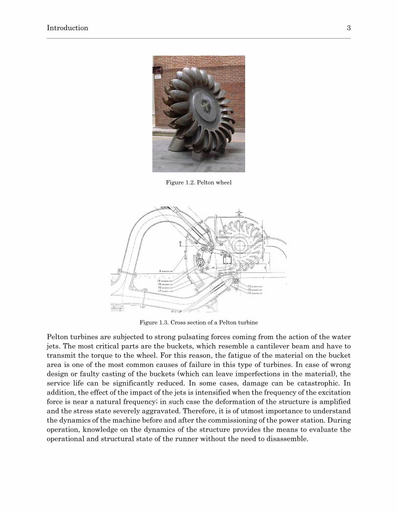
Figure 1.2. Pelton wheel ........................................................................................................... 3
Figure 1.3. Cross section of a Pelton turbine ........................................................................... 3
Figure 2.1. Bode plot when the system enters in resonance with an external force [38] ......12
Figure 2.2. Main dimensions of a Pelton runner ....................................................................13
Figure 2.3. Correlation between head 𝐻 and specific speed 𝑁𝑠 [8] ........................................14
Figure 2.4. Views of the Pelton unit........................................................................................16
Figure 2.5. Left, view of the runner and right, CAD geometry of the runner .......................16
Figure 2.6. Front and rear view of the meshed bucket ...........................................................18
Figure 2.7. Pure bucket modes ................................................................................................19
Figure 2.8. Pure bucket modes ................................................................................................20
Figure 2.9. Mesh sensitivity analysis .....................................................................................21
Figure 2.10. Left: Mesh of the whole runner, right: detailed mesh of the buckets ................21
Figure 2.11. Runner modes .....................................................................................................23
Figure 2.12. Runner modes 2 ..................................................................................................24
Figure 2.13. Impact test setup ................................................................................................25
Figure 2.14. Accelerometers disposition on the hanged runner .............................................26
Figure 2.15. FRF’s and coherence after impacts in the tangential (red) and axial (blue)
directions .................................................................................................................................28
Figure 2.16. ODS of some tangential modes of the suspended runner ..................................29
Figure 2.17. Numerical and experimental modes of a Pelton runner. Top, numerical
results and bottom, response spectrum after the impacts .....................................................30
Figure 2.18. Frequencies of a disk and of a disk with masses ...............................................31
Figure 2.19. Relative deformation of the outer periphery modes in: left, the disk and
right, the disk with masses .....................................................................................................32
Figure 2.20. 2-ND axial deformation of the base of the buckets for every mode shape .........33
Figure 3.1. Sketch of the impact tests performed on the machine .........................................36
Figure 3.2. Position of the accelerometer A31, A34 (left) and A35 and A38 (right) ..............36
Figure 3.3. FRF of the response of accelerometers E1V (green), E2V (blue), E3V (pink)
and E4V (red) to horizontal (top) and vertical (bottom) impacts ...........................................37
Figure 3.4. Numerical model of Pelton rotor ..........................................................................39

vi List of figures
Figure 3.5. First (left) and second (right) horizontal bending modes .....................................39
Figure 3.6. Torsional (left) and third bending (right) modes..................................................40
Figure 3.7. 1-ND (left) and 0-ND (right) rotor/runner modes ................................................40
Figure 3.8. Identification of the modal shapes excited by the hammer impacts ...................41
Figure 3.9. Runner without constraint (left) and runner attached to the shaft (right) .........42
Figure 3.10. Distribution of axial and tangential frequencies for free vibrating and for
attached runner .......................................................................................................................42
Figure 3.11. Left, runner A-1 attached to the machine and left, A-2 buckets with back
supports ...................................................................................................................................43
Figure 3.12. Left, view of the turbine with open housing and right, view of impacts in
the buckets ...............................................................................................................................44
Figure 3.13. Location of the accelerometers on the runner A-2 and the impacts ..................44
Figure 3.14. Axial (red) and tangential (blue) impacts to a bucket of the installed
runner. Top: coherence, bottom: FRF's (amplitude and phase) .............................................45
Figure 3.15. Mode distribution for the experimental Pelton turbine .....................................45
Figure 3.16. Views of Moncabril Pelton unit ..........................................................................47
Figure 3.17. Distribution of accelerometers ............................................................................47
Figure 3.18. Accelerometer position on machine bearings 1 (left), 2 (middle) and 3
(right) .......................................................................................................................................48
Figure 3.19. FRF (bottom) and coherence (top) between accelerometer and hammer
signal to axial (red) and tangential (blue) impacts .................................................................48
Figure 3.20. Distribution of natural frequencies of Moncabril turbine..................................49
Figure 3.21. Geometry of the runners T, K and A ..................................................................49
Figure 3.22. Left, mesh of runner T, and right, distribution of axial frequencies .................50
Figure 3.23. Plot of 𝐷𝑠 against 𝑁𝑠 ...........................................................................................51
Figure 3.24. Runner pitch diameter trend ..............................................................................54
Figure 3.25. Bucket width trend .............................................................................................54
Figure 3.26. Trend between the design of Pelton runners and the natural frequencies .......55
Figure 3.27. Axial natural frequencies of several runners in a non-dimensional form .........56
Figure 4.1. View of experimental setup ..................................................................................60
Figure 4.2. FRF of the response of axial (red) and tangential (blue) accelerometers
placed on bucket 6 to axial impacts on the bucket .................................................................60
Figure 4.3. FRF of the response of A34 (blue) and E4V (green) accelerometers to axial
impacts on the bucket ..............................................................................................................61

List of figures vii
Figure 4.4. FRF of the response of axial (red) and tangential (blue) accelerometers
placed on bucket 6 to axial impacts on the bucket .................................................................61
Figure 4.5. FRF of the response of A34 (blue) and E4V (green) accelerometers to axial
impacts on the bucket ..............................................................................................................61
Figure 4.6. FRF of the response of tangential accelerometers placed on bucket 6 to
tangential impacts on the bucket ............................................................................................62
Figure 4.7. FRF of the response of A34 (blue) and E4V (green) accelerometers to
tangential impacts on the bucket ............................................................................................62
Figure 4.8. FRF of the response of tangential accelerometers placed on bucket 6 to
tangential impacts on the bucket ............................................................................................62
Figure 4.9. FRF of the response of A34 (blue) and E4V (green) accelerometers to
tangential impacts on the bucket ............................................................................................63
Figure 4.10. FRF’s of the response from bearing position A31 (top) and A34 (bottom) to
impacts on bucket 21 in axial (red), tangential (blue) and radial (green) directions .............64
Figure 4.11. FRF’s of the response from bearing positions A35 (top) and A38 (bottom)
to impacts on bucket 21 in axial (red), tangential (blue) and radial (green) directions ........64
Figure 4.12. FFT and coherence between axial accelerometer on the bucket and vertical
position A34 .............................................................................................................................65
Figure 4.13. FRF’s of the response from bearing position A31 (top) and A34 (bottom) to
impacts on bucket 21 in axial (red), tangential (blue) and radial (green) directions .............66
Figure 4.14. FRF’s of the response from bearing position A35 (top) and A38 (bottom) to
impacts on bucket 21 in axial (red), tangential (blue) and radial (green) directions .............66
Figure 4.15. FFT and coherence between tangential accelerometer on the bucket and
position A38 .............................................................................................................................67
Figure 4.16. FRF of the response of bearing positions A31 (top) and A34 (bottom) to
impacts in bucket 21 in axial (red), tangential (blue) and radial (green) directions .............68
Figure 4.17. FRF of the response of bearing positions A35 (top) and A38 (bottom) to
impacts in bucket 21 in axial (red), tangential (blue) and radial (green) directions .............69
Figure 4.18. FRF’s of the response from bearing position A34 (top) and A38 (bottom) to
impacts on bucket 16 in axial (red), tangential (blue) and radial (green) directions .............70
Figure 4.19. FRF’s of the response to impacts on bucket 16 in axial (red), tangential
(blue) and radial (green) direction from bearing positions A31 (top) and A38 (bottom) ........71
Figure 4.20. FRF’s of the response from bearing position A31 (top) and A38 (bottom) to
impacts on bucket 16 in axial (red), tangential (blue) and radial (green) directions .............71
Figure 4.21. FRF of the response of bearing positions A31 (top) and A34 (bottom) to
impacts in bucket 6 in axial (red) and tangential (blue) directions .......................................72
Figure 4.22. Coherence between bearing acc. A34 and bucket 6 acc. ....................................72

viii List of figures
Figure 4.23. FRF of the response of bearing positions A31 (top) and A34 (bottom) to
impacts in bucket 6 in axial (red) and tangential (blue) directions .......................................73
Figure 4.24. Frequencies of the tangential mode for different buckets .................................74
Figure 4.25. Frequencies of the rim mode for different buckets ............................................74
Figure 4.26. FRF’s of the response from bearing positions A13 (top) and A14 (bottom)
to impacts in axial (red) and tangential (blue) directions ......................................................75
Figure 4.27. FRF of the response of bearing positions A13 (top) and A14 (bottom) to
impacts in axial (red) and tangential (blue) directions ..........................................................76
Figure 4.28. FRF of the response of bearing positions A13 (top) and A14 (bottom) to
impacts in axial (red) and tangential (blue) directions ..........................................................76
Figure 4.29. FRF of the response of bearing positions A13 (top) and A14 (bottom) to
impacts in axial (red) and tangential (blue) directions ..........................................................77
Figure 5.1. Sketch of the position of the sensors during on-site measurements ...................80
Figure 5.2. On the left, onboard system installed on the shaft and on the right,
horizontal accelerometers placed on the turbine bearing ......................................................80
Figure 5.3. Screenshot of the SCADA software at minimum load of the turbine ..................81
Figure 5.4. Time signal during the tests from position A34 ...................................................82
Figure 5.5. Time signal during startup transient from A34...................................................83
Figure 5.6. Acceleration waterfall of the startup transient from A34 ...................................84
Figure 5.7. Waterfall of the startup transient from A31 in acceleration m/s2 (top) and
velocity mm/s (bottom) ............................................................................................................85
Figure 5.8. Runner modes excited in the initial impact detected from A31 ..........................87
Figure 5.9. Runner modes excited in the initial impact detected from A34 ..........................87
Figure 5.10. Runner modes from A35 (top) and A38 (bottom) in the initial impact ..............88
Figure 5.11. Transient from shaft accelerometers A2 (top) and A34 (bottom) ......................88
Figure 5.12. Spectra waterfall from strain gauge (bottom), from shaft accelerometer
(middle) and coherence between both signals (top) ................................................................89
Figure 5.13. Startup from position A38 ..................................................................................90
Figure 5.14. Torsional rotor mode detected with the strain gage ..........................................90
Figure 5.15. Axial and tangential modes from positon A34 at the start of the speed-up ......91
Figure 5.16. Axial and tangential modes from positon A34 at the end of the speed-up ........92
Figure 5.17. Velocity time signal from A31(top) and A34 (bottom) ........................................93
Figure 5.18. Overall vibration values during startup from A31 (red) and A34 (blue) ...........93
Figure 5.19. Spectra waterfall from position A34 of Arties at minimum load .......................94

List of figures ix
Figure 5.20. Spectra waterfall from position A31. Top, partial load and bottom, full load
.................................................................................................................................................95
Figure 5.21. Wavelet representation of the signal from A31 at partial load .........................96
Figure 5.22. Waterfall in the band of the axial modes at minimum (top) and maximum
(bottom) load from position A31 ..............................................................................................97
Figure 5.23. Comparison between axial frequencies in the machine still (top), during
part-load operation (middle) and full-load operation (bottom) ...............................................98
Figure 5.24. Excitation of tangential and axial c-ph. modes at minimum (top) and
maximum (bottom) load from position A31 ............................................................................99
Figure 5.25. Wavelet representation of the tangential modes excited from A31 ...................99
Figure 5.26. Excitation of radial modes at minimum (top) and maximum (bottom) load
from position A31 .................................................................................................................. 100
Figure 5.27. Overall RMS velocity values from positions A31 (red), A34 (blue), A35
(green) and A38 (orange) at partial load (left) and full load (right) ..................................... 101
Figure 5.28. Overall RMS velocity values in the band of axial modes from positions A31
(red), A34 (blue), A35 (green) and A38 (orange) at partial load (left) and full load (right)
............................................................................................................................................... 102
Figure 5.29. Overall RMS velocity values in the band of tangential modes from positions
A31 (red), A34 (blue), A35 (green) and A38 (orange) at partial load (left) and full load
(right) ..................................................................................................................................... 102
Figure 5.30. Time signal of the whole test from position A14 .............................................. 103
Figure 5.31. Time signal during the startup transient from A14 ........................................ 104
Figure 5.32. Waterfall of the startup transient from position A14 ...................................... 104
Figure 5.33. Tangential modes excited after the first impact .............................................. 105
Figure 5.34. Axial counter-phase modes after initial impact ............................................... 106
Figure 5.35. Startup from position A13 ................................................................................ 106
Figure 5.36. Tangential modes from position A14. Bottom, start of speed-up .................... 107
Figure 5.37. Tangential modes at the end of the transient .................................................. 107
Figure 5.38. Axial modes at the end of the transient ........................................................... 108
Figure 5.39. Overall velocity vibration levels from A13 ....................................................... 108
Figure 5.40. Spectra waterfall from A14 after the impingement of the second jet .............. 109
Figure 5.41. Overall RMS velocity values during second jet transient ................................ 110
Figure 5.42. Spectra waterfall at minimum (top) and maximum load (bottom) from
position A14 ........................................................................................................................... 111
Figure 5.43. Wavelet of the vibration from A14 at the lower frequency range .................... 112
x List of figures
Figure 5.44. Wavelet waterfall of the vibration from A13 at the lower frequency range .... 112
Figure 5.45. Range of runner axial modes at minimum (top) and maximum load
(bottom) .................................................................................................................................. 113
Figure 5.46. Range of the tangential modes at minimum (top) and maximum load
(bottom) .................................................................................................................................. 114
Figure 5.47. Wavelet waterfall in the range 800-1000Hz .................................................... 114
Figure 5.48. Range of the axial c.-phase modes at minimum (top) and maximum load
(bottom) .................................................................................................................................. 115
Figure 5.49. Overall RMS levels for different monitoring locations. Left, at minimum
load and right, at maximum load .......................................................................................... 116
Figure 6.1. Sketch of a monitoring system ........................................................................... 121
Figure 6.2. Dynamic model to determine the response in the monitoring positions to the
excitation generated during the operation of the machine................................................... 122
Figure 6.3. Trend analysis of a spectral band detecting damage, the diagnostic and the
repair ..................................................................................................................................... 122
Figure 6.4. Mapping showing the evolution of condition indicator levels with operating
conditions (power and head) in a pump-turbine ................................................................... 123
Figure 6.5. Vibration generation sketch ............................................................................... 124
Figure 6.6. Typical spectral vibration signature in a Pelton turbine ................................... 125
Figure 6.7. ISO 10816-5. Group 1 horizontal machines with vibration limits ..................... 125
Figure 6.8. Spectral bands in a Pelton turbine spectrum ..................................................... 126
Figure 6.9. Particle erosion in Pelton turbine components .................................................. 128
Figure 6.10. Typical fatigue cracks in Pelton runners ......................................................... 129
Figure 6.11. Injector needle damage by erosion (left) and cavitation (right) ....................... 129
Figure 6.12. Injector damage in Pelton turbine .................................................................... 129
Figure 6.13. Examples of blockage in Pelton turbine injectors ............................................ 130
Figure 6.14. Examples of weld repair ................................................................................... 130
Figure 6.15. Change of a worn runner .................................................................................. 131
Figure 6.16. Distribution of the forces produced by the jet on a bucket (image taken
from [30]) ............................................................................................................................... 132
Figure 6.17. Trend plot of the overall vibration values measured in the turbine bearing
............................................................................................................................................... 134
Figure 6.18. Frequencies acquired by the monitoring system in the turbine bearing ........ 134
Figure 6.19. Pictures of the wheel with damage. Left, view of the broken bucket and
right, detached bucket part ................................................................................................... 135

List of figures xi
Figure 6.20. Displacement and distribution of stresses on the bucket with a misaligned
jet ........................................................................................................................................... 135
Figure 6.21. Variation in the runner 𝑓𝑓 band and 𝑓𝑏 band levels with time ...................... 137
Figure 6.22. Variation in one of the rotor natural frequencies band levels with time ........ 137
Figure 6.23. Variation in one of the runner axial and tangential frequency band levels
with time ................................................................................................................................ 137
Figure 6.24. Incipient detection ............................................................................................ 138
Figure 6.25. Data driven approach ....................................................................................... 139

xii List of figures

List of tables
Table 2.1. Characteristics of Arties Pelton turbine ................................................................16
Table 2.2. Information about the FEM simulation of the runner ..........................................20
Table 2.3. Variation in the bucket frequencies for different modes .......................................32
Table 3.1. Mesh characteristics of the shaft and the alternator ............................................38
Table 3.2. Elasticity of the bearings in every direction ..........................................................38
Table 3.3. Comparison between experimental and numerical rotor modes ...........................41
Table 3.4. Axial frequencies in the old runner and the new runner ......................................46
Table 3.5. Tangential frequencies in the old runner and the new runner .............................46
Table 3.6. Characteristics of Moncabril Pelton turbine ..........................................................47
Table 3.7. Main features of Pelton turbines available ............................................................51
Table 4.1. Axial RMS acceleration values between bucket 21 and monitoring positions ......65
Table 4.2. Tangential RMS acceleration values between bucket 21 and monitoring
positions ...................................................................................................................................67
Table 4.3. Axial RMS acceleration values between bucket 21 and monitoring positions ......68
Table 4.4. Radial RMS acceleration values between bucket 21 and monitoring positions
.................................................................................................................................................69
Table 4.5. Axial RMS acceleration values between bucket 16 and monitoring positions ......70
Table 4.6. Axial RMS acceleration values between bucket 6 and monitoring positions ........73
Table 5.1. Overall RMS velocity values of Arties from different monitoring positions ....... 101
Table 5.2. Averaged RMS values for the axial modes from every position at partial and
full load .................................................................................................................................. 101
Table 5.3. Averaged RMS values for the tangential modes from every position at partial
and full load ........................................................................................................................... 102
Table 5.4. Overall RMS velocity levels from different monitoring positions at minimum
and maximum load ................................................................................................................ 115

xiv List of tables

Nomenclature
𝑎 Bucket height mm
𝑏 Bucket width mm
𝐶 Damping coefficient kg · s−1
𝐶𝑐 Critical damping coefficient kg · s−1
𝐶0 Water jet velocity m · s−1
𝐷1 Pitch diameter mm
𝐷𝑠 Specific diameter
𝑑𝑜 Nozzle diameter mm
𝐸 Specific energy m2 · s−2
𝐹 External force N
𝑓 Natural frequency Hz
𝑓𝑏 Bucket passing frequency Hz
𝑓𝑓 Rotation frequency Hz
𝑓𝑝 Pole passing frequency Hz
𝑔 Gravitational acceleration m · s−2
𝐻 Head m
𝐾 Stiffness constant kg · s−2
𝑘𝐶𝑚 Nozzle loss coefficient
𝑘𝑢 Peripheral velocity coefficient
𝑀 Mass kg
𝑛 Integer number
𝑁 Rotational speed min−1
𝑁11 Unit speed
𝑁𝑠 Specific speed
𝑃 Rated output kW
𝑄 Discharge m3 · s−1
𝑄11 Unit discharge
𝑆 Power spectrum
𝑇 Time period s

xvi Nomenclature
𝑈1 Peripheral velocity m · s−1
𝑢 Position m
�̇� Velocity m · s−1
�̈� Acceleration m · s−2
𝑧0 Number of nozzles
𝑧𝑏 Number of buckets
Greek symbols
∆ Sampling interval s
𝜅 Coherence
𝜉 Damping ratio
𝜙 Phase angle °
{𝜙} Eigenvector
𝜔 Angular frequency rad · s−1
𝜔𝑛 Angular natural frequency rad · s−1
Abbreviations
AI Artificial Intelligence
CAD Computer Assisted Design
DFT Discrete Fourier Transform
DOF Degrees of Freedom
EMA Experimental Modal Analysis
FEA Finite Element Analysis
FFT Fast Fourier Transformation
FRF Frequency Response Function
FT Fourier Transform
ND Nodal Diameter
ODS Operational Deflection Shape
RMS Root Mean Square

Chapter 1 Introduction
1.1. Introduction
1.1.1. The future of hydropower
Hydropower is one of the most important renewable energies. It has been used since the 19th
century to generate electricity by means of rotational machines called turbines, which convert
the potential energy of the water into mechanical energy. The technology and design of
hydraulic turbines has been developed and optimized to the extent of providing efficiencies
of over 90%, which is one of the largest among all power generation machines. The future of
hydropower is closely tied to the evolution of the so-called new renewable energies (NRE),
like solar and wind. These technologies have been largely developed in the last years and are
characterized by its low environmental impact compared to other established technologies
like nuclear or thermic energy. Due to the increasing concern about the environmental effects
of power generation, NRE are taking the lead to a more sustainable future and are
experiencing a rapid increase [1]. Nevertheless, the energy generated depends on the
atmospheric conditions and it is random. This is translated into a growing share of electricity
production that comes from intermittent sources, and cannot be adapted to the actual
electricity demand. In order to ensure the balance between supply and demand, hydropower
installations are required to fill the fluctuating gap. This requires power plant operators to
increase the operating range of hydraulic turbines and to undergo more starts and stops,
what leads to a faster deterioration of the turbine components, especially the runner.
This new scenario enhances the action of the forces applied on the rotating equipment and
can put at risk its structural integrity. Since hydropower machines are designed to be a
reliable and profitable investment for the power utility and its owners, it is therefore
essential to understand the dynamics of the machine and to use this knowledge to track and
monitor their performance during its service life. In doing so, faulty operating conditions or

2 Introduction
deterioration of the machine can be detected and power plant operators can take convenient
action.
Figure 1.1. Evolution of installed worldwide hydropower capacity [2]
1.1.2. Operation of Pelton turbines
The Pelton turbine is one of the most efficient types of turbines. It is used in power stations
where the hydraulic head is high, usually above 400 m, and operates with low discharges.
Pelton turbines have efficiencies that exceed 90% for a wide operating range, thus being one
of the most efficient and flexible type of hydraulic turbine [3]. There is a wide range of
capacities and dimensions of Pelton runners and the most powerful ones are those housed in
the Bieudron power station in Switzerland, with a rated output of 423 MW each [4], [5].
The invention of the Pelton turbine dates back to the end of the 19th century. In the late
1870’s, Lester Allan Pelton (1829-1908), a fortune seeker who was established in California
during the Gold Rush, found that the performance of a water wheel could be improved by
adding a middle ridge to the buckets. In that way, the water flow was split and deflected,
what caused a stronger impulse on the buckets due to a better utilization of the energy of the
water. In addition, Pelton found that the performance of the machine was increased when
the water flow impinged the buckets at maximum velocity. At present, a Pelton runner
consists of a casted stainless steel disk with a series of metal cups divided in halves attached
along its periphery (see Figure 1.2). They are classified as impulse turbines because they
have no pressure difference between the inlet and the outlet, what means only the kinetic
energy of the water is employed to impulse the runner. In consequence, all the potential
energy of the water (hydraulic head) must be converted into velocity before entering the
turbine. This is attained by means of a nozzle, which is installed at the end of the penstock
and directed in the tangential direction of the wheel (see Figure 1.3). By doing so, the high
speed water jet ejected from the nozzle impinges the buckets of the runner perpendicularly.
Introduction 3
Figure 1.2. Pelton wheel
Figure 1.3. Cross section of a Pelton turbine
Pelton turbines are subjected to strong pulsating forces coming from the action of the water
jets. The most critical parts are the buckets, which resemble a cantilever beam and have to
transmit the torque to the wheel. For this reason, the fatigue of the material on the bucket
area is one of the most common causes of failure in this type of turbines. In case of wrong
design or faulty casting of the buckets (which can leave imperfections in the material), the
service life can be significantly reduced. In some cases, damage can be catastrophic. In
addition, the effect of the impact of the jets is intensified when the frequency of the excitation
force is near a natural frequency; in such case the deformation of the structure is amplified
and the stress state severely aggravated. Therefore, it is of utmost importance to understand
the dynamics of the machine before and after the commissioning of the power station. During
operation, knowledge on the dynamics of the structure provides the means to evaluate the
operational and structural state of the runner without the need to disassemble.
4 Introduction
1.2. Interest of the study
The study proposed is of great interest in the industrial field. With the surge of new
renewables, Pelton turbines are required to work under harsher operating conditions, which
put at risk the integrity of the runner. Apart from the efforts performed in the stage of design
to reduce the effect of the pulsating forces on the structure, several factors can compromise
the Remaining Useful life (RUL) of the machine that cannot be predicted beforehand.
Scenarios such as a damaged runner or abnormalities in the jet quality can remain unnoticed
for as much time it requires undergoing a machine inspection. Having a deep understanding
of the dynamics of the machine and knowing how this is affected by the aforementioned
undesired conditions opens the door to surveilling what is happening inside the machine in
real time and provides facility operators a major control on their assets.
1.3. State of the art
First records on the dynamic behavior of Pelton turbines can be tracked back to the start of
the 20th century. In 1937, Fulton [6] stated that with the steady increase in output of Pelton
turbines, there had been an outbreak of cracks due to bucket vibration, which caused
designers to reinforce their designs. In the 1950s, many catastrophic failures caused by
fatigue fracture took place due to the trend of increasing size and power of Pelton turbines
[7]. In the following years, bolted buckets started being replaced by new designed one piece
casted runners. Even though the existence of bucket vibration was acknowledged, mainly the
static stresses coming from centrifugal forces and the jet impact were considered being
important [8].
In the following years, the attention to the alternating stresses coming from the dynamic
excitation of the buckets started to rise. One of the most important publications was written
by Grein et al. [9], who remarked the importance of the dynamic stresses as a controlling
parameter for fatigue failure and considered the bucket vibration in circumferential direction
to be the most dangerous natural vibration, whose amplification factor in case of resonance
could reach up to x1000. The buckets of Pelton turbines had to be designed carefully to limit
the maximum value of alternating stresses due to dynamic excitation to 45 MPa in order to
avoid fatigue and to guarantee the minimum service life requirements [10]. Before the
development of numerical methods, the design criteria to ensure long lifetime regarding the
fatigue problem was established by performing laboratory tests and crack propagation
calculations based on theory of fracture mechanics [11]. The use of strain gauges was also a
spread practice in order to study the vibrations of the buckets [12].
With the development of Finite Element Methods, the dynamic behavior of the buckets could
be more accurately studied. The structural analysis of Pelton turbines is nowadays an
indispensable procedure to be followed during the manufacturing of Pelton turbines. Many
publications mention the study of the natural frequencies in such stage [13][14]. In the
upgrading and the maintenance of Pelton turbines also many publications can be found
addressing the study of the stress fluctuations [15][16]. Failure analyses can also be found

Introduction 5
[17]. A better knowledge of the stress state of the Pelton turbines also lead to the development
of new technologies which have allowed optimizing the fabrication of Pelton runners
[18][19][20], and new designs in order to decrease the effect of alternating stresses [21][22].
The traditional method in the analysis of the vibration of the runners was based on the
classical beam theory, which consisted in treating the bucket as a beam clamped at its base.
With the increase in size an output, the development of more sophisticated models are
necessary, such as in the case of Bieudron power plant [23].
Due to the discrepancies between the natural frequencies in the theoretical design and the
real runner, Schmied et al. [24] developed a method to detune a Pelton runner by finding the
optimal bucket mass removal required. In this article, other modes of a Pelton bucket are
briefly described: torsional mode, axial mode and radial mode. It is also stated that as the
number of nodal diameters increases, so does the resemblance to a pure bucket mode. Sick et
al. [25] highlight the difficulties in performing quasi-static stress analysis nowadays and
divides the general practice in structural analysis of Pelton turbines in two steps: first the
deformation and stress in the bucket as a response to the dynamic load and second the
analysis of natural modes and frequencies and evaluation of safety limits with respect to
resonance.
In the last years, some authors performed test measurements with strain gauges [26], [27]
and pressure sensors [28]–[32] on reduced models to determine the pressure distribution, the
values of the jet force and the stresses at the critical locations of the buckets in case of
resonance. The natural frequencies of the buckets were determined by experimental testing
with accelerometers and were analyzed with FEM analysis.
On his review on dynamic problems of Francis and Pelton turbines, Brekke [33] still alerted
of the appearance of superimposed high frequency bucket oscillations, which can put at risk
the whole turbine even before damage can be detected in an inspection.
Sanvito et al. [34] developed a new method for identifying the dynamic stresses of Pelton
turbines, which consisted in decoupling the load on the bucket into different harmonic
analyses and then reconstructing the ‘stress vs. time’ trace. This was performed on the
reduced geometry of a Pelton bucket, which consisted of one half constrained by its contact
surfaces, for no description of the runner modes was available.
In 2007, Pesatori et al. [35] performed a numerical and experimental analysis of a two jets
Pelton turbine. A FEM model consisting of a single bucket was studied with different
boundary conditions on the periodic surfaces. Experimental tests showed that the behavior
of a runner bucket was best defined by a bucket whose periodic surfaces were clamped. In
this publication, also the first five modes of the bucket were described. However, the behavior
of the whole runner is not described.
The vibration and mechanical effects on Pelton turbines are well documented by Dörfler [36].
In his book, the author warns about the important role of the harmonics of the excitation
frequency on the dynamic stresses due to the low damping ratio of the natural oscillations of
the runner/bucket assembly. With this, taking into account the effect of the added mass and
the precision in the machining are indispensable to avoid resonances. Dörfler also explains

6 Introduction
in detail the importance of a proper choice of jet distribution and the number of buckets due
to its effect on the vibrations of the whole machine, in transient and normal operation. Special
attention is put on the torsional modes of the rotor, which are highly excited during startup.
Records on monitoring of Pelton turbines are difficult to find. One relevant publication is
written by Karacolcu et al. [37], who explain the procedure followed in the rehabilitation of a
two jet horizontal Pelton turbine, which suffered from strong vibrations at certain output (30
MW), even though its rated power was of 38 MW. In the mechanical assessment of the
existing turbine, vibration data was analyzed, finding a strong vibration in the axial bearings
at 150 Hz. After performing bump tests on the buckets and turbine casing and doing a FEM
analysis, a rotor-bending mode was found near the problematic frequency. Even though the
most important rotor modes were showed in the paper, runner modes were not described.
1.4. Objectives
The main objective of this thesis is to obtain a deeper understanding of the dynamic behavior
of horizontal Pelton turbine prototypes in operation. The ultimate purpose is to use the
research results to improve the capability to monitor the condition of the turbines in real
time.
To accomplish this, the first goal is to have a better understanding of the structural (modal)
response of Pelton runners when still and in operating conditions (mounted in the machine
and rotating). The purpose is also to check the ability to extrapolate the results to different
Pelton turbines.
The second goal is to study the feasibility to monitor the runner vibrations from typical
monitoring positions in the bearings. For that purpose, the propagation of the runner
vibrations to the monitoring positions have to be evaluated.
Finally, to improve the existing monitoring procedures, it is necessary to analyze the data
from monitoring several Pelton units and to determine the main types of damage found in
these machines and the symptoms observed in the spectra.
1.5. Outline
This thesis is organized in three parts. The first part contains a deep modal analysis of Pelton
turbines, the second shows the study of the transmissibility of runner vibrations to the
monitoring positions and the third part is focused on the study of the dynamic behavior of
these turbines with a proposal to improve condition monitoring.
The first part consists of two chapters. In chapter two the modal behavior of a Pelton runner
without constraints (free vibrating body) is studied numerically and experimentally. Then a
discussion on the parameters that influence on the natural frequencies and modal shapes is
performed. In chapter three, three modal analyses are carried out for whole Pelton machines.

Introduction 7
The first analysis is performed numerically with the geometry of the runner of the previous
section. The second and the third are made experimentally on two different Pelton turbines.
Finally, all the results are brought together with data obtained from other Pelton turbines to
define general trends in the modal behavior of Pelton turbines.
The second part is developed in chapter four. In this chapter the excitability of the runner
modes and the transmissibility of the bucket vibrations to the monitoring positions is studied
in the same Pelton machines whose modal behavior was studied in the previous section.
The third part comprises chapter five and six. In chapter five the dynamic behavior of both
Pelton turbines is studied during the startup transient and under different loads. In chapter
six, the vibration signatures of different Pelton turbines are analyzed in order to extract the
symptoms of common types of damage. Then an update on the spectral bands and vibration
amplitudes is proposed as condition indicators for a possible improvement of condition
monitoring of Pelton turbines.

8 Introduction
Chapter 2 Modal behavior of Pelton runners
To perform the dynamic analysis of a Pelton turbine it is essential to understand its modal
characteristics. This chapter is devoted to analyzing numerically and experimentally the
natural frequencies and mode shapes of a Pelton runner without constraints. To do so, the
numerical model of a real suspended runner has been created. First, the mode shapes of a
single bucket have been identified and classified. After that, the frequencies and mode shapes
have been analyzed for the whole structure. An Experimental Modal Analysis (EMA) has
been performed on the runner to check the validity of the numerical model. Finally, the
results have been discussed and the influence of different geometrical parameters on the
modal behavior of the runner has been analyzed.
2.1. Theoretical background
The modal analysis of a structural system consists in determining its inherent vibration
properties, such as its natural frequencies and mode shapes. Modal analysis is fundamental
when studying any dynamic system because it allows determining how it responds to external
excitations and helps preventing it from reaching resonance.
2.1.1. Free vibration of a structural system
To introduce the basics of modal analysis, we will consider a dynamic system with a single
degree of freedom (DOF) composed by a mass attached to a spring and a damper. The
vibration of this system is governed by the second law of Newton, which is expressed as
follows [38]
𝑀�̈� + 𝐶�̇� + 𝐾𝑢 = 𝐹(𝑡) Eq. 2.1

10 2.1 Theoretical background
The first term on the left side of the equation represents the inertial forces of the system, the
second term the friction forces (dissipation of energy) and the third the elastic forces, where
𝑀 is the mass, 𝐶 is the damping coefficient and 𝐾 is the stiffness constant. �̈�, �̇� and 𝑢 represent
the acceleration, the velocity and the position of the mass, at every instant respectively. The
term on the right side of the equation, 𝐹(𝑡), represents an external force applied on the system
as a function of time.
When the force applied on the system is removed, the motion of the system is described as a
free vibration, and is written as follows
𝑀�̈� + 𝐶�̇� + 𝐾𝑢 = 0 Eq. 2.2
The solution to this equation allows obtaining the natural frequency of the system 𝜔𝑛. If we
consider that the friction forces are negligible, then we obtain the following expression
𝜔𝑛 = √𝐾 𝑀⁄ Eq. 2.3
There are three possible solutions to Eq. 2.3 depending on whether the system is
underdamped (𝐶 2𝑀⁄ < 𝐾 𝑀⁄ ), critically damped (𝐶 2𝑀⁄ = 𝐾 𝑀⁄ ) or overdamped (𝐶 2𝑀⁄ >
𝐾 𝑀⁄ ). The value of 𝐶 when the system is critically damped is called the coefficient of critical
damping 𝐶𝑐. The damping ratio is written as
𝜉 = 𝐶
𝐶𝑐⁄ Eq. 2.4
The previous equations describe the motion of a single DOF dynamic system. However, any
real structural system has infinite DOF’s. This can also be represented in a simplified way
as multiple masses connected between them with springs and dampers. The motion of such
structural system with an applied loading is governed by the following equation:
[𝑀]{�̈�} + [𝐶]{�̇�} + [𝐾]{𝑢} = 𝐹(𝑡) Eq. 2.5
Where [𝑀] is the mass matrix, [𝐶] is the damping matrix and [𝐾] the stiffness matrix. {�̈�},{�̇�}
and {𝑢} are respectively the acceleration vector, velocity vector and the position vector. F(t)
is the external force applied on the system. All vectors vary as a function of time.
The natural frequencies and mode shapes of the system can be found if Eq. 2.5 is formulated
supposing zero damping and no applied loading. In such case, the equation of motion reduces
to:
[𝑀]{�̈�} + [𝐾]{𝑢} = 0 Eq. 2.6
This is known as the free vibration equation of motion. In this case, only the inertial and the
elastic forces are significant.

Modal behavior of Pelton runners 11
To solve the equation, we assume a harmonic solution of the following form:
{𝑢} = {𝜙} sin𝜔𝑡 Eq. 2.7
Where {𝜙} is the eigenvector or mode shape and 𝜔 is the circular frequency. This solution
means that the inertial forces are equal to the elastic forces and that all the degrees of
freedom of the vibrating structure move in a synchronous manner. When this solution is
differentiated and substituted in Eq. 2.7, the following is obtained:
−𝜔2[𝑀]{𝜙} sin𝜔𝑡 + [𝐾]{𝜙} sin𝜔𝑡 = 0 Eq. 2.8
Which is simplified to the following form:
([𝐾] − 𝜔2[𝑀]){𝜙} = 0 Eq. 2.9
There are two possible solutions for Eq. 2.9. The first one implies that {𝜙} = 0, which does
not provide any valuable information from the physical point of view. The second one is
obtained by solving the following expression:
𝑑𝑒𝑡([𝐾] − 𝜔2[𝑀]) = 0 Eq. 2.10
And provides a set of discrete 𝜔2 values and their corresponding eigenvectors {𝜙𝑖}. These
values describe the free vibration of the dynamic system. Each eigenvalue represents one
natural frequency of the system by the following relationship:
𝑓𝑖 =
𝜔𝑖
2𝜋 Eq. 2.11
Where 𝑓𝑖 is the i-th natural frequency of the system. The natural frequencies are those at
which the elastic forces counterbalanced the inertial forces, and the mode shapes describe
the deflection shape of the system at each natural frequency.
2.1.2. Forced vibration of a structural system
When studying the forced vibration of a structural system with a single DOF, we consider
that the force applied is oscillating harmonically, leaving Eq. 2.1 in the following way:
𝑀�̈� + 𝐶�̇� + 𝐾𝑢 = 𝐹0sin(𝜔𝑡 + 𝜑) Eq. 2.12
Where 𝐹0 is the amplitude of the force and 𝜑 is the phase angle difference between the
frequency of the excitation force and the frequency of the system. The steady-state solution
of the equation is as follows:
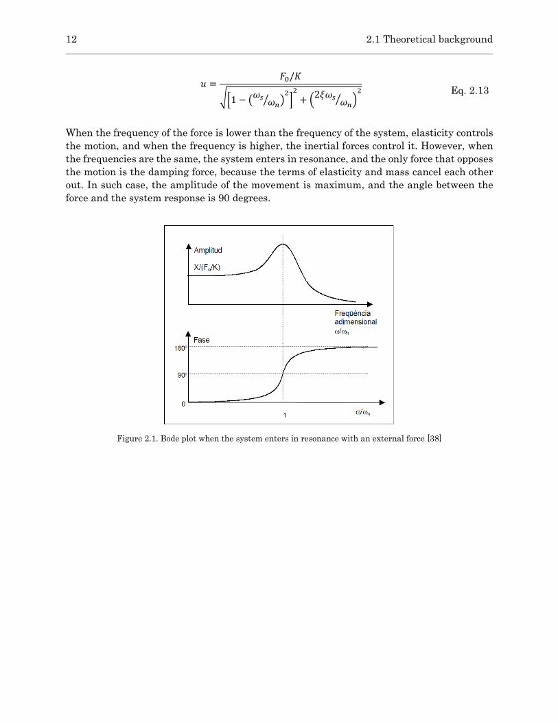
12 2.1 Theoretical background
𝑢 =
𝐹0/𝐾
√[1 − (𝜔𝑠
𝜔𝑛⁄ )
2]2
+ (2𝜉𝜔𝑠
𝜔𝑛⁄ )
2
Eq. 2.13
When the frequency of the force is lower than the frequency of the system, elasticity controls
the motion, and when the frequency is higher, the inertial forces control it. However, when
the frequencies are the same, the system enters in resonance, and the only force that opposes
the motion is the damping force, because the terms of elasticity and mass cancel each other
out. In such case, the amplitude of the movement is maximum, and the angle between the
force and the system response is 90 degrees.
Figure 2.1. Bode plot when the system enters in resonance with an external force [38]

Modal behavior of Pelton runners 13
2.2. Structure of a Pelton runner
2.2.1. Geometry
The geometry of a Pelton turbine runner is very different from reaction turbines. It is
composed by a wheel with a series of buckets attached to its periphery. The buckets are the
components that receive the impact of the water jet and where the hydraulic energy is
converted into mechanical energy. The shape of a Pelton bucket must meet a compromise
between a hydraulic and a structural optimal shape; one the one hand, they must be
dimensioned and contoured to have maximum hydraulic efficiency and on the other hand
they must guarantee enough structural resistance to bear the forces applied to them during
operation. The main dimensions of a Pelton runner are showed in Figure 2.2. The pitch
diameter 𝐷1 is defined as double the distance between the jet axis and the runner centerline,
𝑏 is the bucket width and 𝑎 is the bucket height. The main parts of the buckets are the cutout,
the splitter and the rim. The cutout is where the jet first enters the bucket, the splitter divides
the jet into two streams, and the rim is where the water last interacts with the turbine and
is considered the outlet of the bucket. Between the splitter and the rim, the water jet is
deflected almost 180 degrees to deliver the maximum available power to the turbine.
Figure 2.2. Main dimensions of a Pelton runner
2.2.2. Specific speed and dimensions
The dimensions of the wheel and the buckets of a Pelton turbine are related to its specific
speed. The specific speed 𝑁𝑠 of a turbine is a non-dimensional number that represents the
speed at which a geometrically similar turbine that delivers an output of 1 kW rotates under
a head of 1 m. It is a widely used parameter to classify hydraulic turbines and to define their
compactness. Over the years, there has been a trend to increase the specific speed of Pelton
turbines due to economic reasons [39]: minimizing the dimensions of the runner leads to a
reduced cost on electro-mechanical equipment and on civil works. Nevertheless, factors such
as cavitation and the maximum allowable peripheral velocity of the runner define the upper
limit of the specific speed value [10]. These effects are dramatized with increasing head

14 2.2 Structure of a Pelton runner
because of the increasing velocity of the jet. It is possible to correlate the head of the turbine
to its specific speed, as shown in the chart of Figure 2.3.
Figure 2.3. Correlation between head 𝐻 and specific speed 𝑁𝑠 [8]
The main dimensions of the runner can be related to the specific speed by the following
procedure. The equation of specific speed 𝑁𝑠 for a one jet Pelton runner is expressed as follows
𝑁𝑠 = 𝑁𝑃0,5𝐻−1,25 Eq. 2.14
In this equation, 𝑁𝑠 represents the specific speed in min-1, 𝑁 the rotational speed in min-1, 𝑃
is the rated output in kW and 𝐻 is the net head in m. These values can be directly related to
the dimensions of the nozzle and of the wheel when some assumptions are made. Since almost
all the potential energy in a Pelton turbine is converted into kinetic energy, the velocity 𝐶0 of
the water at the exit of the nozzle can be defined as
𝐶0 = 𝑘𝐶𝑚√2𝑔𝐻 Eq. 2.15
Where 𝑘𝐶𝑚 is the loss coefficient of the nozzle and amounts to 0,95 to 0,98, 𝑔 is the
gravitational acceleration in m· s-2 and 𝐻 is the net head in m. To obtain maximum power
from the water jet, the peripheral velocity of the buckets 𝑈1 at the pitch diameter must be
half the absolute velocity 𝐶0 of the water jet. In practice, this value can range from 0,44 to
0,46 and it is defined by 𝑘𝑢.
𝑈1 = 𝑘𝑢𝐶0 = 𝑘𝑢𝑘𝐶𝑚√2𝑔𝐻 Eq. 2.16
For simplification purposes we will consider 𝑘𝐶𝑚=1 and 𝑘𝑢=0,5.
𝑈1 ≅ √𝑔𝐻2⁄ Eq. 2.17

Modal behavior of Pelton runners 15
We can say then that the velocity 𝑈1 of the bucket only depends on the net head. The diameter
of the runner is related to the rotational speed 𝑁 and the velocity of the bucket 𝑈1 by the
following equation
𝐷1 =
𝑈160
𝜋𝑁 Eq. 2.18
Where 𝑁 is the rotational speed in min-1 and can only take synchronous values, which usually
are 1000, 750, 600, 500 and 428 min-1. The discharge of the Pelton runner can be obtained
from the area of the cross-section of the jet and the jet velocity
𝑄 =𝜋𝑑0
2𝐶04
Eq. 2.19
where 𝑄 is the turbine discharge in m3· s-1 and 𝑑0 is the diameter of the water jet in m.
Substituting the terms 𝑁, 𝑃 and 𝐻 in the Eq. 2.14, we have the following equation
𝑛𝑠 = (𝑈160
𝜋𝐷1)(𝛾
𝜋𝑑02𝐶04
2𝑈12
𝑔)
0,5
(2𝑈1
2
𝑔)
−1,25
Eq. 2.20
If we consider that 𝐶0 = 2 · 𝑈1 we have
𝑛𝑠 = 𝑐𝑜𝑛𝑠𝑡.
𝑑0𝐷1
Eq. 2.21
It can be seen that the ratio of the diameter of the jet 𝑑0 to the diameter of the runner 𝐷1 is
of major importance. From these two parameters, all the other design parameters can be
deduced from geometrical relationships that are limited by efficiency and/or structural
resistance reasons. For example, the centripetal stresses increase with the mass of the bucket
(which is proportional to 𝑑0) and with the centripetal acceleration (which is inversely
proportional to 𝐷1) for a given head. The bending stresses also increase with increasing
bucket size and decreasing pitch diameter, so the ratio 𝑑0/𝐷1 must be decreased with
increasing head.
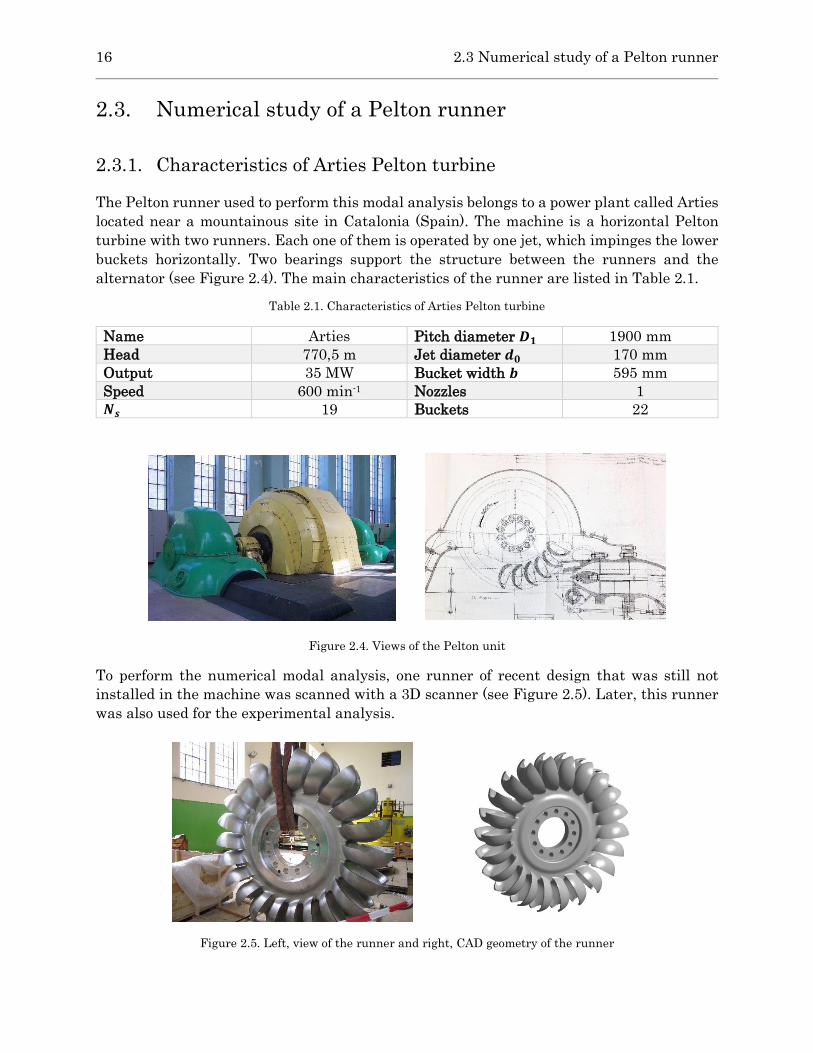
16 2.3 Numerical study of a Pelton runner
2.3. Numerical study of a Pelton runner
2.3.1. Characteristics of Arties Pelton turbine
The Pelton runner used to perform this modal analysis belongs to a power plant called Arties
located near a mountainous site in Catalonia (Spain). The machine is a horizontal Pelton
turbine with two runners. Each one of them is operated by one jet, which impinges the lower
buckets horizontally. Two bearings support the structure between the runners and the
alternator (see Figure 2.4). The main characteristics of the runner are listed in Table 2.1.
Table 2.1. Characteristics of Arties Pelton turbine
Name Arties Pitch diameter 𝑫𝟏 1900 mm
Head 770,5 m Jet diameter 𝒅𝟎 170 mm
Output 35 MW Bucket width 𝒃 595 mm
Speed 600 min-1 Nozzles 1
𝑵𝒔 19 Buckets 22
Figure 2.4. Views of the Pelton unit
To perform the numerical modal analysis, one runner of recent design that was still not
installed in the machine was scanned with a 3D scanner (see Figure 2.5). Later, this runner
was also used for the experimental analysis.
Figure 2.5. Left, view of the runner and right, CAD geometry of the runner

Modal behavior of Pelton runners 17
2.3.2. Finite Element Analysis (FEA)
The numerical study of the Pelton turbine has been performed by means of Finite Element
Analysis (FEA). FEA is a powerful computational technique that allows simulating the
physical behavior of any structure by decomposing its domain into a finite number of
subdivisions and converting it into a mathematical model. These subdomains, called
elements, are connected to each other by nodes, which specify the location in space where
degrees of freedom and interaction between the elements exist. The interaction between the
elements is defined by systematic approximate solutions of the governing physical equations
that affect the structure, which are constructed by applying variational or weighted residual
methods.
The program used to perform this analysis is the commercial software ANSYS®. It provides
a wide range of modules, suitable to perform different kinds of structural analysis. For this
study, the Modal Analysis module was used to obtain the natural frequencies and mode
shapes of the turbine.
The first step when performing a FEA is to discretize the domain of the structure into a finite
number of elements. Such procedure is known as meshing and largely defines the quality of
the results of the simulation. Increasing the amount of elements and nodes (what is known
as a refined mesh) usually improves the accuracy of the simulation. However, having a large
number of mesh elements implies a greater computational effort. Therefore, it is convenient
to perform a mesh sensitivity analysis in order to find a balance between result stability and
reasonable computational time. Equally important is to assess a proper mesh refinement
depending on the characteristics of the geometry. Those areas of the solid that have high
curvatures require a finer mesh than those with small geometric variations.
After meshing the geometry, the boundary conditions of the body must be determined. For
structural analysis, this usually means to fix one or more areas of the body. When performing
a free vibration analysis, no boundary conditions are considered.
2.3.3. Numerical analysis of a single bucket
The geometry of the Pelton runner was imported to ANSYS®. From the original geometry,
one of the buckets was cut off and treated as a separate body to perform the following
analysis. The meshing of the bucket was carried out with tetrahedral elements, which were
smaller in the areas of the cut-out and the ridge of the bucket due to their high curvature.
The purpose of this study is to know which are the typical mode shapes of a bucket when it
is attached to the runner. Hence the model of the bucket wasn’t treated as a free body.
Instead, the body was constrained (zero displacement) on the areas that are attached to the
rest of the runner (see green surfaces in Figure 2.6). The x-direction corresponds to the
tangential direction of the pitch diameter of the runner, y-direction to the radial direction
and z-direction to the axial direction. The mesh had 25000 tetrahedral elements. The mesh
density was increased in the sharp edges and the locations were typically a high
concentration of stresses occur, which are the cutout and the ridge.

18 2.3 Numerical study of a Pelton runner
Figure 2.6. Front and rear view of the meshed bucket
Next, the pure mode shapes of the bucket have been analyzed. Although the number of modes
is infinite for any structure, only the eight modes at the lowest frequencies have been
considered for this study. Since the main dimensions of a bucket are standardized in relation
to the jet diameter, we can take the results as representative for most Pelton runners. In
Figure 2.7 front and side views of the first four modes of the bucket are displayed. The regions
that vibrate with maximum amplitude are represented in red while the regions with
minimum or zero displacement are represented in blue. It is worth noting that the color scale
is not the same for all the modes, since the program takes as a reference the maximum and
minimum values of every mode. The shape of the bucket without deformation is depicted with
the light-wired figure.
The first two modes (top left and top right of Figure 2.7) can be compared to the first natural
mode of a cantilever beam, in which the structure tilts over a clamped base. The first one is
known as axial mode, because the bucket bends in the same direction as the axis of the
runner. The second mode is referred to as tangential mode (or bending mode in
circumferential direction in some publications [24]) and is considered the most dangerous
mode in a Pelton runner since it is the most excited by the impact of the water jet. The bucket
axial mode is found at the lowest frequency because the stiffness of the bucket is lower in the
axial direction than in the tangential direction. For both mode shapes, the tips of the bucket
deform in phase.
In the second group of modes (bottom left and bottom right of Figure 2.7), both halves of the
bucket oscillate with opposite phases. In the third mode, which has been named counter-
phase tangential mode but it is also known as torsional mode, the bucket halves bend
tangentially in opposite phases, thus giving certain torsion around the radial axis of the
bucket. In this mode shape, we can also see that the splitter is deforming. The fourth natural
mode, called counter-phase axial mode or rim mode, involves the axial deformation of the
rims of the bucket in opposite directions, with a periodic spreading and contracting motion.

Modal behavior of Pelton runners 19
Axial mode Tangential mode
Counter-phase tangential mode Counter-phase axial mode
Figure 2.7. Pure bucket modes
In Figure 2.8 the fifth, sixth, seventh and eighth natural modes of the bucket have been
represented. All of them are featured by the appearance of transversal nodes on the bucket,
what increases the stiffness, and thus the frequency. In the fifth and sixth modes (top left
and top right of Figure 2.8, respectively) the tips of the bucket are stretched in the radial
direction, with equal and opposed phases on both halves, respectively. Consequently, they
have been named radial and counter-phase radial. The deformation of the rims in the axial
direction is also relevant in these modes.
The seventh mode (bottom left of Figure 2.8) is similar to the counter-phase radial mode,
although the tips of the bucket do not have a pure radial deformation. Instead, they have a
combination of axial and radial deformation. Thus, this mode has been named counter-phase
axial-radial mode. At this frequency, the splitter also shows a large deformation. In the
eighth mode, called 2-ND radial mode, two transversal nodes appear in the bucket and the
tips stretch radially.

20 2.3 Numerical study of a Pelton runner
Radial mode Counter-phase radial mode
Counter-phase radial-axial mode Radial mode with two nodes
Figure 2.8. Pure bucket modes
2.3.4. Numerical analysis of the whole runner
After representing the pure modes of a bucket, the modal simulation of the whole structure
was carried out. A mesh sensitivity analysis was done prior to the analysis to determine an
acceptable number of mesh nodes, which didn’t require too much time and computational
resources, and guaranteed stable results. As seen in Figure 2.9, the values of the first natural
frequencies obtained with different mesh refinements were compared. From 400000 elements
on, the values converged. The main characteristics of the final simulation are listed in Table
2.2. Two views of the mesh are displayed in Figure 2.10. The mesh properties at the buckets
were the same as in the single bucket model.
Table 2.2. Information about the FEM simulation of the runner
Boundary conditions Free body
Material Stainless steel
Density 7500 kg· m-3
Young’s modulus 2 × 10¹¹
Mesh element type Tetrahedral
Number of mesh elements 400000

Modal behavior of Pelton runners 21
Figure 2.9. Mesh sensitivity analysis
Figure 2.10. Left: Mesh of the whole runner, right: detailed mesh of the buckets
0,998
1,000
1,002
1,004
1,006
1,008
1,010
1,012
1,014
0 200000 400000 600000 800000 1000000
f/f*
[-]
Number of Elements [-]
2ND
3ND
4ND

22 2.3 Numerical study of a Pelton runner
Next, the modal shapes of the Pelton runner, which are displayed in Figure 2.11 and Figure
2.12, will be analyzed. The order of appearance of the mode shapes is the same as in the pure
bucket modes. The simulation shows that for every mode shape found in the single bucket,
several variants of the same mode appear in the runner. Each variant of the same bucket
mode appears at a different frequency and combines the oscillation of the buckets and the
wheel in different ways. These can be classified by the number of nodal diameters of the
wheel. The nodal diameters delimit circumferentially consecutive regions oscillating in
opposite phases and have minimum or zero displacement. The areas that are the furthest
from the nodal lines show the maximum deformation amplitude. The number of buckets
determine the total sum of variants of the same bucket mode shape. This Pelton turbine has
22 buckets, thus there is a total amount of 22 modal shapes for every bucket mode, which
reach a maximum number of 11 nodal diameters. For simplicity purposes only the modal
shapes of the Pelton runner with two (2-ND), five (5-ND) and ten (10-ND) nodal diameters
have been displayed for each bucket mode.
The axial, tangential and counter-phase tangential are displayed in Figure 2.11. The color
scale is fixed for every mode to see the differences in amplitude between the different
variants. At the lowest frequencies, one finds the axial modes, where wheel and buckets are
deforming in the axial direction (top of Figure 2.11). When the number of nodes increases
(left to right), the deformation of the disk is minimized and only a deformation in the area of
the buckets is noticed. In that case, the maximum deformation, which is found at the tip of
the buckets, is increased with respect to lower ND modes. The second group (middle of Figure
2.11) corresponds to the tangential modes. The disk deforms in the radial direction for the
first ND modes, while for higher ND only the bending of the buckets is significant, just like
in the axial case. In the third group (bottom of Figure 2.11), the counter-phased tangential
mode involves the movement of the bucket tips in opposite phases. In this case, there is no
deformation of the disk in the 2-ND (only the buckets are oscillating), and the maximum
deformation of the tips of the buckets is kept almost constant for different ND, unlike the
previous cases.
In Figure 2.12, the following modes of the Pelton runner are displayed also for 2-ND, 5-ND
and 10-ND. One can clearly identify the 2-ND runner deformation in all of them, except in
the radial mode, in which the oscillation amplitude of the disk is much lower than the
buckets. In the counter-phase axial modes, the deformation of the disk is in the radial
direction, like in the tangential modes. However, in the counter-phase radial mode, the disk
deforms in the axial direction. In all of them, the deformation of the tip/rim of the buckets
increases with the number of nodal diameters.

Modal behavior of Pelton runners 23
Axial modes
2 ND 5 ND 10 ND
Tangential modes
2 ND 5 ND 10 ND
Counter-phase tangential modes
2 ND 5 ND 10 ND
Figure 2.11. Runner modes

24 2.3 Numerical study of a Pelton runner
Counter-phase axial modes
2 ND 5 ND 10 ND
Radial modes
2 ND 5 ND 10 ND
Counter-phase radial mode
2 ND 5 ND 10 ND
Figure 2.12. Runner modes 2

Modal behavior of Pelton runners 25
2.4. Experimental Modal Analysis (EMA)
The aim of the experimental tests was to study the pure mode shapes and frequencies of the
Pelton runner, without the influence of the rotor. Therefore, the runner was suspended with
a rope and placed in an accessible location of the power station to carry out impact tests. This
was equivalent to considering the runner as a free body (without any constraint) due to the
small influence of the rope on the vibration of the runner.
2.4.1. Impact testing
The object of an Experimental Modal Analysis (EMA) is to determine the frequencies and
mode shapes of a structure experimentally. The procedure consists in executing a series of
impacts to the structure in order to excite its natural frequencies, and in recording the
resulting vibration with accelerometers. Tests can be performed either by placing several
accelerometers on different locations of the structure or by executing several impacts on
different locations. The latter is known as roving hammer method and the results obtained
are the same as if using many accelerometers due to the reciprocity principle. Following any
of these procedures, the natural frequencies and mode shapes of the structure can be
determined.
The instrumentation used during an EMA typically includes an instrumented hammer,
accelerometers and a recording module (Figure 2.13). The hammer is used to excite the
natural frequencies of the structure and, due to an internal sensor, also measures the
magnitude of the force exerted. Accelerometers convert the mechanical motion of the
structure into an electrical signal. The force and the acceleration signals are then recorded
by an acquisition module as a function of time for further analysis.
Figure 2.13. Impact test setup
The sensors used were industrial K-Shear® accelerometers from KISTLER type 8752A50.
Their sensitivity was 100 mV/g and the acceleration range ± 50 g. They were mounted on
clean and flat locations of the runner to ensure reliable and accurate measurements. The

26 2.4 Experimental Modal Analysis (EMA)
sensitivity of the hammer was 223 µV/N. The acquisition module was a LAN-XI Data
Acquisition Hardware from Brüel & Kjær. The model had 12 channels to connect the sensors.
To perform the EMA it was important to choose the location of the sensors accurately to
represent the main mode shapes of the runner. For this reason, four accelerometers were
placed on the surface of the disk (axial direction) with approximately 90 degrees between
them and the same radial position. In addition, four accelerometers were placed on different
locations of the buckets to detect the axial, tangential and radial modes. The axial
accelerometers were adhered on the outer surface of the bucket rim, approximately in the
middle section, and the tangential and radial accelerometers were placed on the tip of the
bucket, on perpendicular surfaces. Since the vibration of a runner is complex, different series
of impacts were carried out. In each series, the accelerometers were relocated in different
parts of the buckets. One distribution to detect tangential modes of the runner is displayed
in Figure 2.14.
Figure 2.14. Accelerometers disposition on the hanged runner
2.4.2. Signal processing
After performing the impact tests, the recorded data is analyzed in order to obtain the
information.
The Fourier transform (FT) is a powerful tool that decomposes a signal into a series of
frequencies by which it is formed [40]. The FT of a function 𝑓(𝑥) is the function 𝐹(𝜔), where
𝐹(𝜔) = ∫ 𝑓(𝑥)𝑒−𝑖𝜔𝑥𝑑𝑥∞
−∞
Eq. 2.22

Modal behavior of Pelton runners 27
And the inverse Fourier transform is
𝑓(𝑥) =1
2𝜋∫ 𝐹(𝜔)𝑒𝑖𝜔𝑥𝑑𝜔∞
−∞
Eq. 2.23
When we think of 𝑓(𝑥) as a signal, then the function 𝐹(𝜔) is called the signal’s spectrum. The
spectrum represents the energy of vibration in the frequency domain.
Since the signals obtained from the impact tests are discrete and periodic, it is not necessary
to perform the FT. Instead, we use the Fast Fourier Transform (FFT), which is a fast
algorithm for computing the Discrete Fourier Transform (DFT). The DFT is written as
𝐴𝑘 = ∑ 𝑒−𝑖
2𝜋𝑁𝑘𝑛𝑎𝑛
𝑁−1
𝑛=0
Eq. 2.24
Where the analyzed signal is 𝑎𝑛 for 𝑛 = 0…𝑁 − 1, and 𝑎𝑛 = 𝑎𝑛+𝑗𝑁 for all 𝑛 and 𝑗. The FFT
computes the DFT at a lower cost. Once the spectrum of a signal is obtained, the natural
frequencies are easily detected by peak picking.
The Frequency Response Function (FRF) gives the magnitude ratio and phase difference
between the vibration of the structure and the excitation force. It can be thought of as the
transfer function between the output (structure vibration) and the input (excitation force) of
a dynamic system. With FRF the resonant frequencies, the damping and the mode shapes
can be obtained [41].
The FRF are obtained from the steady-state solution of the equation of the forced vibration
(section 2.1.2) and can be expressed in terms of magnitude and phase angle 𝜙 in the following
manner:
|𝑋(𝜔)
𝐹(𝜔)| = [
1
𝑘] [
𝜔𝑛2
√(𝜔𝑛2 −𝜔2)2 + (2𝜉𝜔𝜔𝑛)
2] Eq. 2.25
𝜙 = tan−1 [
2𝜉𝜔𝜔𝑛
𝜔𝑛2 −𝜔2
] Eq. 2.26
The coherence function compares the content of two different signals to assess which
frequencies are of the same origin. To define the coherence, it is necessary to first introduce
the concept of power spectrum and cross-spectrum [42].
The power spectrum 𝑆𝑥𝑥,𝑗 of a signal 𝑥 indicates the amplitude of a periodic oscillation in the
frequency domain. It is defined by the following equation:
𝑆𝑥𝑥,𝑗 = (2∆2 𝑇⁄ )𝑋𝑗𝑋𝑗∗ Eq. 2.27

28 2.4 Experimental Modal Analysis (EMA)
Where 𝑋𝑗 is the Fourier transform of 𝑥 at frequency 𝑓𝑗(𝑋𝑗), 𝑋𝑗∗ is its complex conjugate, ∆ is
the sampling interval and 𝑇 is the total duration of the recording.
In a similar fashion, the cross-spectrum between two signals 𝑥 and 𝑦 is defined in the
following way:
< 𝑆𝑥𝑦,𝑗 >=
2∆2
𝑇
1
𝐾∑𝑋𝑗,𝑘𝑌𝑗,𝑘
∗
𝐾
𝑘=1
Eq. 2.28
In this case, we replace the conjugate of the FT of signal , 𝑋𝑗∗, with the conjugate of the FT of
signal 𝑦, 𝑌𝑗,𝑘∗ . The subscript 𝑘 and letter 𝐾 represent the number of trials. Finally, the
coherence can be expressed in the following way:
< 𝜅𝑥𝑦,𝑗 >=
| < 𝑆𝑥𝑦,𝑗 > |
√< 𝑆𝑥𝑥,𝑗 > √< 𝑆𝑦𝑦,𝑗 > Eq. 2.29
The coherence measures the relationship between two signals x and y at the same frequency
and ranges between 0 and 1 at every frequency, in which 0 means there is no coherence
between both signals, and 1 means absolute coherence between them at that frequency.
2.4.3. Results
An example of the FRF’s obtained after performing hammer impacts to one runner bucket in
the tangential and axial direction is shown in the top plot of Figure 2.15. The coherence
between the hammer signal (excitation) and the accelerometers (response) is shown in the
bottom plot of Figure 2.15.
400
[Hz]
600
[Hz]
800
[Hz]
1k
[Hz]
1
2
3
4
5
-140
20
[(m/s^2)/N] Cursor values
X: 853.500 Hz
Y(Mg):22.256m (m/s^2)/N
y(Ph):164.150 degrees
4
400
[Hz]
600
[Hz]
800
[Hz]
1k
[Hz]
0.2
0.4
0.6
0.8
1[] Cursor values
X: 938.000 Hz
Y: 0.993
4
Figure 2.15. FRF’s and coherence after impacts in the tangential (red) and axial (blue) directions

Modal behavior of Pelton runners 29
To identify the modal shapes of the structure, it is necessary to compare the signals from the
different accelerometers (or different impacts) in terms of magnitude and phase. For complex
structures it is common to create a simplified virtual model known as Operating Deflection
Shapes (ODS), which offers a dynamic representation of the vibration pattern of the
structure. Many nodes compose this model and each one of them represents the motion
detected from one accelerometer. Some runner modes are represented in the ODS model in
Figure 2.16.
Figure 2.16. ODS of some tangential modes of the suspended runner

30 2.5 Analysis and discussion of results
2.5. Analysis and discussion of results
This section attempts to analyze the modes of a Pelton runner by comparing the vibrational
modes of the wheel with those of a single bucket. The interaction between both elements will
be studied in order to have a better understanding of the modal behavior of the turbine. In
Figure 2.17, the frequencies obtained from the numerical model (upper chart) can be
compared with the experimental results (lower chart). Every type of bucket mode shape is
attributed a color to relate more easily the peaks from the experimental tests with the
numerical modes. The modes studied are located in a range between 0 and 1200 Hz. The first
modes found are the axial modes between 195 Hz and 473 Hz. They are followed by the
tangential modes (in-phase and counter-phase), which appear between 519 and 591 Hz and
overlap each other. Next, the counter-phase axial modes are found in a very narrow frequency
range between 618 and 648 Hz. The counter-phase radial modes and the radial modes are
found in the next frequency band, being the former ones spread over a wide range of
frequencies and the latter concentrated in a narrow band (1017 to 1077 Hz). Similar to the
counter-phase axial modes, the counter-phase radial-axial modes have small differences
between them.
Figure 2.17. Numerical and experimental modes of a Pelton runner. Top, numerical results and bottom,
response spectrum after the impacts
A noticeable fact is the nonlinear increase of the frequencies of each mode, which are
distributed in a similar way to an asymptote. The modes in lower frequencies are those with
a fewer number of runner nodal diameters. As the number of nodal lines increases, so does
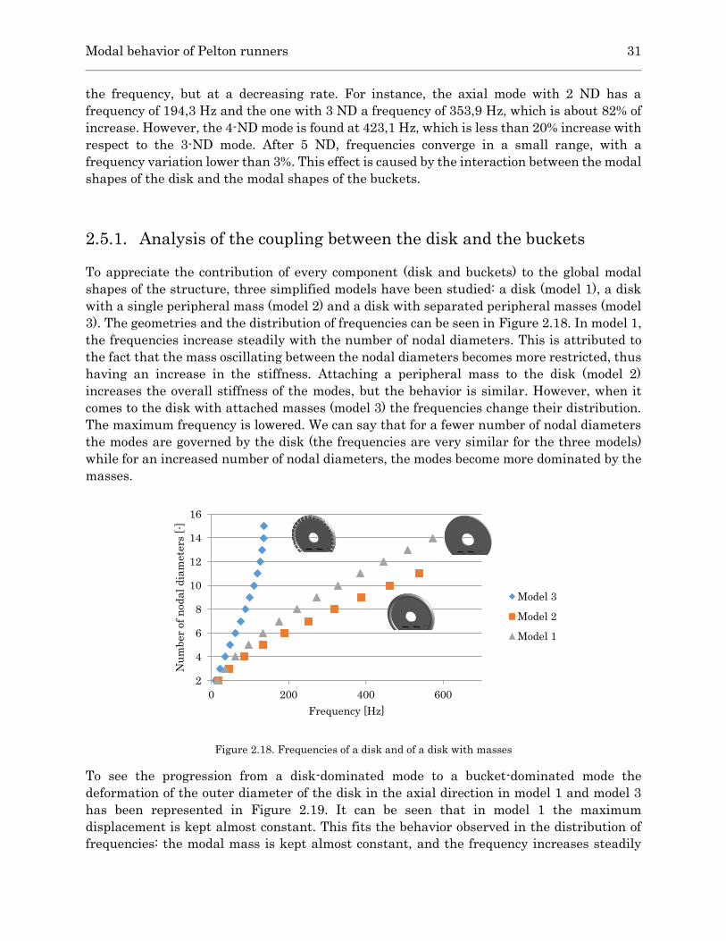
Modal behavior of Pelton runners 31
the frequency, but at a decreasing rate. For instance, the axial mode with 2 ND has a
frequency of 194,3 Hz and the one with 3 ND a frequency of 353,9 Hz, which is about 82% of
increase. However, the 4-ND mode is found at 423,1 Hz, which is less than 20% increase with
respect to the 3-ND mode. After 5 ND, frequencies converge in a small range, with a
frequency variation lower than 3%. This effect is caused by the interaction between the modal
shapes of the disk and the modal shapes of the buckets.
2.5.1. Analysis of the coupling between the disk and the buckets
To appreciate the contribution of every component (disk and buckets) to the global modal
shapes of the structure, three simplified models have been studied: a disk (model 1), a disk
with a single peripheral mass (model 2) and a disk with separated peripheral masses (model
3). The geometries and the distribution of frequencies can be seen in Figure 2.18. In model 1,
the frequencies increase steadily with the number of nodal diameters. This is attributed to
the fact that the mass oscillating between the nodal diameters becomes more restricted, thus
having an increase in the stiffness. Attaching a peripheral mass to the disk (model 2)
increases the overall stiffness of the modes, but the behavior is similar. However, when it
comes to the disk with attached masses (model 3) the frequencies change their distribution.
The maximum frequency is lowered. We can say that for a fewer number of nodal diameters
the modes are governed by the disk (the frequencies are very similar for the three models)
while for an increased number of nodal diameters, the modes become more dominated by the
masses.
Figure 2.18. Frequencies of a disk and of a disk with masses
To see the progression from a disk-dominated mode to a bucket-dominated mode the
deformation of the outer diameter of the disk in the axial direction in model 1 and model 3
has been represented in Figure 2.19. It can be seen that in model 1 the maximum
displacement is kept almost constant. This fits the behavior observed in the distribution of
frequencies: the modal mass is kept almost constant, and the frequency increases steadily
2
4
6
8
10
12
14
16
0 200 400 600
Nu
mb
er
of
nod
al
dia
mete
rs [
-]
Frequency [Hz]
Model 3
Model 2
Model 1

32 2.5 Analysis and discussion of results
due to the stiffness increase. However, in model 3 the deformation of the disk decreases
largely between 2 ND and 4 ND. From 5 ND the deformation barely shows a reduction. Some
conclusions can thus be extracted from the chart. First, the increase in disk nodal diameters
from 2 ND to 4 ND happens to reduce largely the vibrating mass of the disk, which explains
the large difference between the first frequencies. Second, for modes with more than 5 ND
the deformation of the disk is very small and shows almost no variation, even if the number
of nodal diameters is increased. It can be thus said that in the higher modes almost all the
vibration is performed by the buckets, and that their base is similarly restricted. This allows
explaining why all the frequencies are so similar. Therefore, when studying the runner, the
mode in the highest frequency, which corresponds to 11 ND, has the most resemblance to a
pure bucket mode. The base of the bucket has the smallest angle between nodal diameters,
being the most rigid one.
Figure 2.19. Relative deformation of the outer periphery modes in: left, the disk and right, the disk with masses
To check the similarity of the 11-ND mode to a simple bucket vibration, another analysis has
been performed. The natural frequencies of a single bucket and the natural frequencies
obtained in the 11-ND runner mode are indicated in Table 2.3. Comparing both columns, it
can be seen that the bucket-dominated frequencies of the runner are 1-4.5% lower than the
constrained bucket, which means that the nodal diameter provides more flexibility than a
rigid surface. It is worth noting, though, that the variation in the frequencies differs from one
mode shape to another. The axial and the counter-phase radial mode shapes are the most
affected by the change in the boundary conditions of the disk.
Table 2.3. Variation in the bucket frequencies for different modes
Single bucket
[Hz]
Runner 11 ND
[Hz]
Axial 487,8 473,7
Tangential 564,9 558,2
Tangential c-ph. 590,9 591,2
Axial c-ph. 635,0 648,6
Radial c-ph. 1120,4 1082,3
Radial 1091,9 1077,9
-1
-0,5
0
0,5
1
0 100 200 300
Rela
tive d
efo
rma
tion
[%
]
Circumferential node position [°]-1
-0,5
0
0,5
1
0 100 200 300
Rela
tive d
efo
rma
tion
[%
]
Circumferential node position [°]
2ND
3ND
4ND
5ND
6ND

Modal behavior of Pelton runners 33
2.5.2. Effect of the bucket mode shapes
As already indicated, the effect of the coupling to the disk affects differently on every bucket
mode. Some of them converge in a small range, like tangential and counter-phase axial
modes. Such behavior can be attributed to the nature of the deformation of the bucket and
its interaction with the disk. Some modes require a low contribution of the disk, for example
the counter-phase axial modes, which are local and only affect the rim of the buckets. For
these types of modes, a change in the stiffness of the coupling to the disk has a small effect
on the vibration of the buckets. On the other hand, it is also important to mention that the
increase in the number of nodal diameters affects the stiffness in the axial direction. In
circumferential and radial direction, the disk is very stiff and the increase in nodal diameters
does not entail a big change. Therefore, the modes with a large axial deformation of the disk
(see axial and counter-phase radial in Figure 2.11 and Figure 2.12) are more sensitive to the
variation in the disk stiffness. Tangential and counter-phase axial modes have a significant
deformation of the disk but in the radial direction. In Figure 2.20, the deformation of the
runner of 2-ND mode shapes at the base of the buckets in the axial direction has been plotted
for all the modes. It is clear that the axial and counter-phase radials are the mode shapes
most influenced by the axial stiffness of the disk.
Figure 2.20. 2-ND axial deformation of the base of the buckets for every mode shape
-0,5
-0,4
-0,3
-0,2
-0,1
0
0,1
0,2
0,3
0,4
0,5
0 100 200 300
Defo
rma
tion
[m
m]
Circumferential node position [°]
Axial
Tangential
Tangential c-ph.
Axial c-ph.
Radial c-ph.
Radial
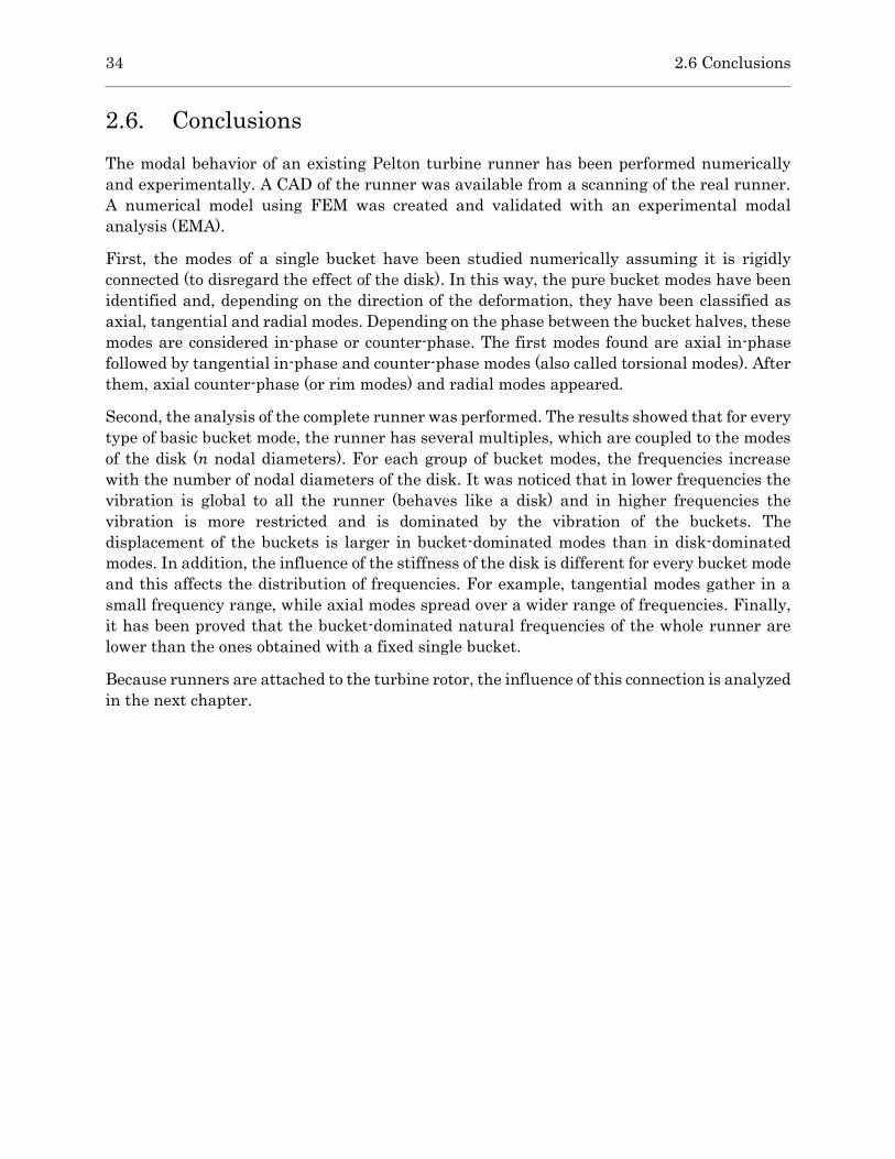
34 2.6 Conclusions
2.6. Conclusions
The modal behavior of an existing Pelton turbine runner has been performed numerically
and experimentally. A CAD of the runner was available from a scanning of the real runner.
A numerical model using FEM was created and validated with an experimental modal
analysis (EMA).
First, the modes of a single bucket have been studied numerically assuming it is rigidly
connected (to disregard the effect of the disk). In this way, the pure bucket modes have been
identified and, depending on the direction of the deformation, they have been classified as
axial, tangential and radial modes. Depending on the phase between the bucket halves, these
modes are considered in-phase or counter-phase. The first modes found are axial in-phase
followed by tangential in-phase and counter-phase modes (also called torsional modes). After
them, axial counter-phase (or rim modes) and radial modes appeared.
Second, the analysis of the complete runner was performed. The results showed that for every
type of basic bucket mode, the runner has several multiples, which are coupled to the modes
of the disk (𝑛 nodal diameters). For each group of bucket modes, the frequencies increase
with the number of nodal diameters of the disk. It was noticed that in lower frequencies the
vibration is global to all the runner (behaves like a disk) and in higher frequencies the
vibration is more restricted and is dominated by the vibration of the buckets. The
displacement of the buckets is larger in bucket-dominated modes than in disk-dominated
modes. In addition, the influence of the stiffness of the disk is different for every bucket mode
and this affects the distribution of frequencies. For example, tangential modes gather in a
small frequency range, while axial modes spread over a wider range of frequencies. Finally,
it has been proved that the bucket-dominated natural frequencies of the whole runner are
lower than the ones obtained with a fixed single bucket.
Because runners are attached to the turbine rotor, the influence of this connection is analyzed
in the next chapter.

Chapter 3 Modal behavior of Pelton machines
In the previous chapter, the modal behavior of a Pelton runner was comprehensively studied
with the support of numerical models and experimental data. In the real machine, though,
the runner is attached to the shaft, and this has an influence on its natural frequencies.
Moreover, a Pelton turbine comprises the runner, the shaft and the alternator, which behave
as a single body and have their own modal shapes and eigenfrequencies. All of these must be
studied, since they are prone to be excited during the operation of the turbine. For such
purpose, the modal behavior of the real turbine is analyzed in this chapter with the help of
impact tests on the installed machine and with a numerical model of the whole rotor.
Next, to check if the distribution of runner modes obtained previously is similar between
different Pelton turbines, two machines with different specific speeds are studied
experimentally.
After that, the effect of the mechanical and hydraulic design on the modal behavior of Pelton
turbines is studied. Two machines with the same characteristics and specific speed but
different structural design are analyzed to see which influence this has on its natural
frequencies. The effect of hydraulic design is then studied with three turbines with different
specific speed but similar hydraulic design.
Finally, the feasibility to estimate the natural frequencies of Pelton turbines is evaluated. To
that end, Pelton runners are geometrically characterized as function of its operational
features, and the location of their natural frequencies analyzed.
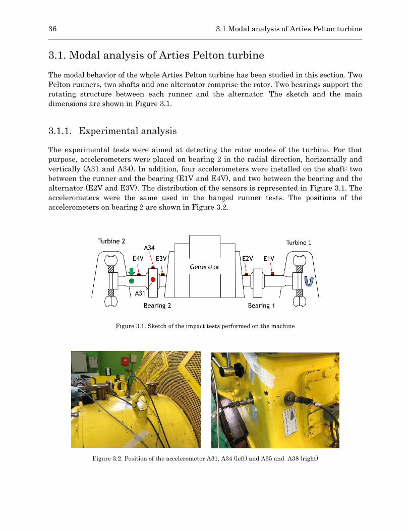
36 3.1 Modal analysis of Arties Pelton turbine
3.1. Modal analysis of Arties Pelton turbine
The modal behavior of the whole Arties Pelton turbine has been studied in this section. Two
Pelton runners, two shafts and one alternator comprise the rotor. Two bearings support the
rotating structure between each runner and the alternator. The sketch and the main
dimensions are shown in Figure 3.1.
3.1.1. Experimental analysis
The experimental tests were aimed at detecting the rotor modes of the turbine. For that
purpose, accelerometers were placed on bearing 2 in the radial direction, horizontally and
vertically (A31 and A34). In addition, four accelerometers were installed on the shaft: two
between the runner and the bearing (E1V and E4V), and two between the bearing and the
alternator (E2V and E3V). The distribution of the sensors is represented in Figure 3.1. The
accelerometers were the same used in the hanged runner tests. The positions of the
accelerometers on bearing 2 are shown in Figure 3.2.
Figure 3.1. Sketch of the impact tests performed on the machine
Figure 3.2. Position of the accelerometer A31, A34 (left) and A35 and A38 (right)
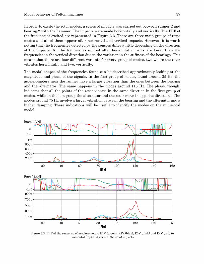
Modal behavior of Pelton machines 37
In order to excite the rotor modes, a series of impacts was carried out between runner 2 and
bearing 2 with the hammer. The impacts were made horizontally and vertically. The FRF of
the frequencies excited are represented in Figure 3.3. There are three main groups of rotor
modes and all of them appear after horizontal and vertical impacts. However, it is worth
noting that the frequencies detected by the sensors differ a little depending on the direction
of the impacts. All the frequencies excited after horizontal impacts are lower than the
frequencies in the vertical direction due to the variation in the stiffness of the bearings. This
means that there are four different variants for every group of modes, two where the rotor
vibrates horizontally and two, vertically.
The modal shapes of the frequencies found can be described approximately looking at the
magnitude and phase of the signals. In the first group of modes, found around 35 Hz, the
accelerometers near the runner have a larger vibration than the ones between the bearing
and the alternator. The same happens in the modes around 115 Hz. The phase, though,
indicates that all the points of the rotor vibrate in the same direction in the first group of
modes, while in the last group the alternator and the rotor move in opposite directions. The
modes around 75 Hz involve a larger vibration between the bearing and the alternator and a
higher damping. These indications will be useful to identify the modes on the numerical
model.
20
[Hz]
40
[Hz]
60
[Hz]
80
[Hz]
100
[Hz]
120
[Hz]
140
[Hz]
160
[Hz]
200u
400u
600u
800u
1m
-140
20
[(m/s^2)/N]
20
[Hz]
40
[Hz]
60
[Hz]
80
[Hz]
100
[Hz]
120
[Hz]
140
[Hz]
160
[Hz]
100u
300u
500u
700u
900u
-140
20
[(m/s^2)/N]
Figure 3.3. FRF of the response of accelerometers E1V (green), E2V (blue), E3V (pink) and E4V (red) to
horizontal (top) and vertical (bottom) impacts

38 3.1 Modal analysis of Arties Pelton turbine
3.1.2. Numerical simulation
A numerical model was developed in order to analyze in detail the modal behavior of a Pelton
turbine. The alternator and the shaft were created by computer assisted design (CAD)
representing the same distribution and dimensions of the real machine. Two models of the
same runner studied in the previous chapter were attached to the tip of the shaft. The design
runner buckets used in the numerical model (from turbine A-1) was different from the ones
installed in the machine (turbine A-2), but the effect of this variance has very low effect on
the modes of the rotor, because it behaves almost as a rigid body.
The numerical model of the turbine (see Figure 3.4) consisted of two runners, two shafts and
the alternator (core and poles). The meshing of the runner geometry had the same
characteristics as the model developed in Chapter 2. The characteristics of the shaft and the
runner are listed in Table 3.1. Two types of connections were used as boundary conditions in
the different components. To attach the runners to the shaft, and the shaft to the alternator,
the contact surfaces were set as bonded connections. These ensure that no translation takes
place between the respective mesh nodes. To emulate the stiffness of the bearings, elastic
connections to the ground (springs) were created in the horizontal and vertical directions.
Table 3.1. Mesh characteristics of the shaft and the alternator
Shaft 1 / Shaft 2 Alternator
Boundary conditions Elastic connect. to ground
Bonded to runner 1 / runner 2
Bonded to alternator
Bonded to shaft 1 and
shaft 2
Material density 7850 kg· m-3 7000 kg· m-3
Young’s modulus 2×10¹¹ 2×10¹¹
Mesh element type Tetrahedral Hexahedral
Number of mesh elements 82300 24800
The procedure followed to know the stiffness of the bearings consisted in varying the
connection elasticities of the FEM model and comparing the resultant frequency values with
the experimental values. The speed dependent oil film elasticity and damping were not
considered. After some calculations, the values listed in Table 3.2 were selected. The
maximum error between experiment and FEM model was under 20% (Table 3.3). The
elasticity values are consistent with results obtained from other studies [43].
Table 3.2. Elasticity of the bearings in every direction
Bearing 1 Bearing 2
Vertical stiffness 5×10⁹ N· m-1 5×10⁹ N· m-1
Horizontal stiffness 3×10⁹ N· m-1 3×10⁹ N· m-1

Modal behavior of Pelton machines 39
Figure 3.4. Numerical model of Pelton rotor
The rotor modes appear in the lowest frequencies and involve all the components of the
turbine, which behave as a single body. In Figure 3.5, the views of the first two horizontal
bending modes of the turbine are shown. Each mode has also a variant in the vertical
direction, at a higher frequency. In the first bending mode the nodes are located by the
bearings, which are the most rigid points of the structure, and the rest of the structure
oscillates around these points. In the second bending mode all the area comprised between
the two bearings acts a node, with a very small oscillation. In fact, the maximum deformation
in this mode shape is found at the tips of the rotor, where the runners are attached. In this
case, the runners behave as a stiff body. There are four variants of this mode depending on
the direction of the deformation (horizontal or vertical), and on the symmetry between both
sides (in-phase and counter-phase).
Figure 3.5. First (left) and second (right) horizontal bending modes
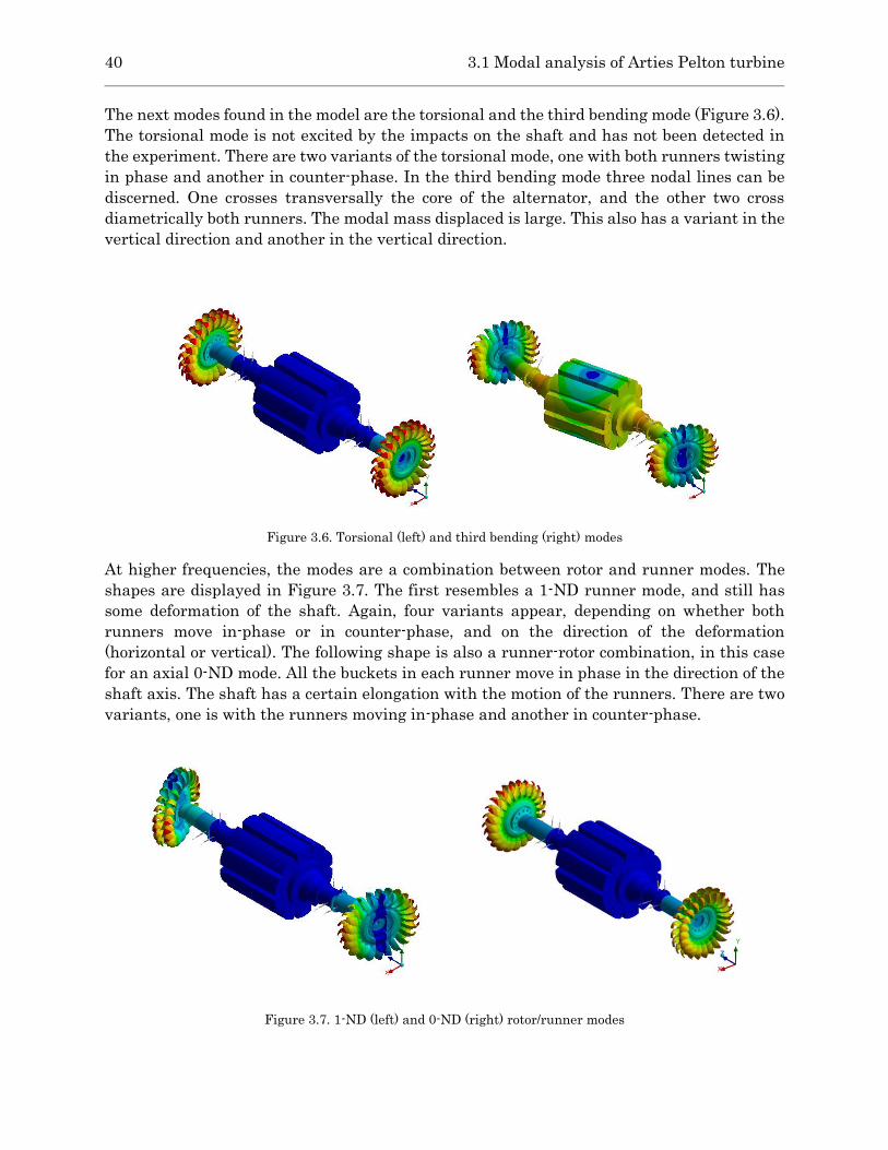
40 3.1 Modal analysis of Arties Pelton turbine
The next modes found in the model are the torsional and the third bending mode (Figure 3.6).
The torsional mode is not excited by the impacts on the shaft and has not been detected in
the experiment. There are two variants of the torsional mode, one with both runners twisting
in phase and another in counter-phase. In the third bending mode three nodal lines can be
discerned. One crosses transversally the core of the alternator, and the other two cross
diametrically both runners. The modal mass displaced is large. This also has a variant in the
vertical direction and another in the vertical direction.
Figure 3.6. Torsional (left) and third bending (right) modes
At higher frequencies, the modes are a combination between rotor and runner modes. The
shapes are displayed in Figure 3.7. The first resembles a 1-ND runner mode, and still has
some deformation of the shaft. Again, four variants appear, depending on whether both
runners move in-phase or in counter-phase, and on the direction of the deformation
(horizontal or vertical). The following shape is also a runner-rotor combination, in this case
for an axial 0-ND mode. All the buckets in each runner move in phase in the direction of the
shaft axis. The shaft has a certain elongation with the motion of the runners. There are two
variants, one is with the runners moving in-phase and another in counter-phase.
Figure 3.7. 1-ND (left) and 0-ND (right) rotor/runner modes

Modal behavior of Pelton machines 41
Finally, all the rotor modes have been identified and the frequencies checked with
experimental results (Table 3.3 and Figure 3.8).
Table 3.3. Comparison between experimental and numerical rotor modes
Horizontal Vertical
Exp. [Hz] Num. [Hz] Error
[%] Exp. [Hz] Num. [Hz]
Error
[%]
2nd bending 33,5 31,54 5,85 36 30,39 15,58
3rd bending 75 79,84 6,45 84 69,0 17,86
4th bending 118 118,22 0,19 120,5 119,57 0,77
20
[Hz]
40
[Hz]
60
[Hz]
80
[Hz]
100
[Hz]
120
[Hz]
140
[Hz]
160
[Hz]
200u
400u
600u
800u
1m
-140
20
[(m/s^2)/N]
Figure 3.8. Identification of the modal shapes excited by the hammer impacts
3.1.3. Runner modes (effect of attachment to the rotor)
In this section, the vibration of the runner when it is attached to the shaft is compared to its
oscillation as a free-vibrating body. In Figure 3.10, the distribution of frequencies of the axial
and the tangential modes are compared between both models. It can be seen that the
frequencies of the runner when it is fixed are higher than when unconstrained, due to the
increased stiffness. Another noticeable fact is that the frequency does not increase in the
same way in all the mode shape variants. The stiffness of the connection affects more the
modes with a lower number of diametrical nodes. This is attributed to the fact that in modes
with less number of ND, the disk dominates the motion, while in modes with higher number
of ND the oscillation is located in the buckets.

42 3.2 Influence of mechanical design (same 𝑁𝑠)
Figure 3.9. Runner without constraint (left) and runner attached to the shaft (right)
Figure 3.10. Distribution of axial and tangential frequencies for free vibrating and for attached runner
3.2. Influence of mechanical design (same 𝑁𝑠)
The main geometrical features of a Pelton turbine are related to its head H, discharge Q and
the number of nozzles. The specific speed is a non-dimensional number used to classify
hydraulic machines, which is defined as
𝑛𝑠𝑞 =𝑁𝑄0.5
𝐸0.75 Eq. 3.1
where 𝑁 is the rotational speed of the turbine, 𝑄 the discharge and 𝐸 the specific energy. The
specific speed 𝑛𝑠𝑞 is related to the head of the turbine and, for Pelton, this is connected to the
ratio between the runner diameter and the jet diameter D/dj. In like manner, the discharge
of the turbine is related to the dimensions of the bucket. Thus the dimensions of a Pelton
2
3
4
5
6
7
8
9
10
11
100 200 300 400 500 600
Nu
mb
er
of
nod
es
[-]
Frequency [Hz]
Axials
Axials (shaft)
Tangentials
Tangentials (shaft)

Modal behavior of Pelton machines 43
runner (from the hydraulic point of view) are characterized by the specific speed 𝑁𝑠. However,
even for the same 𝑁𝑠, runners may bear some differences, especially in the structural design,
depending on the manufacturer and on the year of construction.
In this section, two runners from the same power plant in Arties will be analyzed (turbine A-
1 and turbine A-2). The specific speed 𝑁𝑠 is the same for both (head, discharge, speed and
output), what means they have the same hydraulic design. However, the mechanical design
is different, since they were not produced in the same time, and some mechanical variances
can be discerned. One of the most visible ones is the back shape of the buckets (Figure 3.11).
In the older runner (on the right), the buckets are reinforced with ribs. This was a typical
design feature to make the buckets more resistant to the load of the water jet. In recent
designs (left), the back shape is slimmer. In recent designs, ribs are only to be found in
runners with very high heads.
Figure 3.11. Left, runner A-1 attached to the machine and left, A-2 buckets with back supports
The modal behavior of turbine A-1 was studied in previous sections. An EMA was carried out
in the installed machine as described next to identify the natural frequencies and mode
shapes of the runner A-2.
3.2.1. Experimental tests
The tests were performed systematically on one side of the turbine. The casing of the runner
2 was removed in order to place the sensors and perform the impacts on the buckets (Figure
3.12 left). Three accelerometers were placed on bucket number 21 in the axial, tangential and
radial direction on one side of the bucket, as indicated in Figure 3.12 right and Figure 3.13.
Two accelerometers were placed on buckets 16 and 11 in the axial direction. The
accelerometers used were The procedure consisted in performing impacts on the opposite side
of the buckets, in the axial, tangential and radial directions. Buckets from number 21 to
number 10 were impinged in a row. In this way, most of the modal shapes and natural
frequencies of the runner were identified.
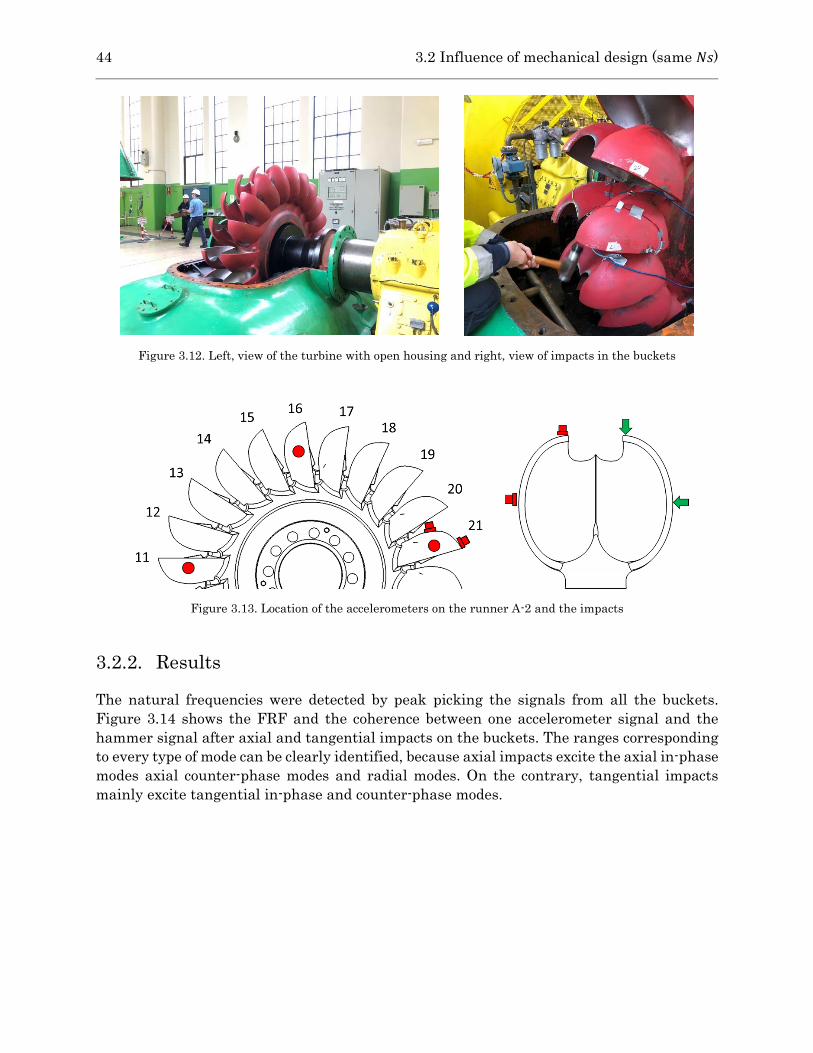
44 3.2 Influence of mechanical design (same 𝑁𝑠)
Figure 3.12. Left, view of the turbine with open housing and right, view of impacts in the buckets
Figure 3.13. Location of the accelerometers on the runner A-2 and the impacts
3.2.2. Results
The natural frequencies were detected by peak picking the signals from all the buckets.
Figure 3.14 shows the FRF and the coherence between one accelerometer signal and the
hammer signal after axial and tangential impacts on the buckets. The ranges corresponding
to every type of mode can be clearly identified, because axial impacts excite the axial in-phase
modes axial counter-phase modes and radial modes. On the contrary, tangential impacts
mainly excite tangential in-phase and counter-phase modes.

Modal behavior of Pelton machines 45
400
[Hz]
600
[Hz]
800
[Hz]
1k
[Hz]
0.2
0.4
0.6
0.8
1[] Cursor values
X: 601.500 Hz
Y: 0.103
4
400
[Hz]
600
[Hz]
800
[Hz]
1k
[Hz]
1
2
3
4
5
-140
20
[(m/s^2)/N] Cursor values
X: 811.000 Hz
Y(Mg):50.832m (m/s^2)/N
y(Ph):-171.055 degrees
4
Figure 3.14. Axial (red) and tangential (blue) impacts to a bucket of the installed runner. Top: coherence,
bottom: FRF's (amplitude and phase)
When representing the frequencies of turbine A-2 with respect to the number of nodes (Figure
3.15), the distribution is very similar to the one of turbine A-1. The order of appearance of
the modes is the same. The axial in-phase and radial counter-phase are still the ones which
are more spread, while the tangential and the axial counter-phase modes are gathered in a
narrow range. However, the values of the frequencies are different, especially the mode
shapes involving a tangential deformation.
Figure 3.15. Mode distribution for the experimental Pelton turbine
2
3
4
5
6
7
8
9
10
11
0 500 1000
Nu
mber
of
nod
es [
-]
Frequency [Hz]
Axial
Tangential
Tangential c-ph.
Axial c-ph.
Radial c-ph.
Radial

46 3.3 Influence of hydraulic design
In Table 3.4, the axial frequencies are listed with the percentage of difference between the
old design and the new design. It can be seen that the frequencies for disk-dominated modes
are similar, while the bucket-dominated modes show an important difference. It can thus be
deduced that the change in the design affects mostly the bucket modes, which in the old
design are stiffer due to the back support. The same behavior can be found in the counter-
phase radial modes. When the tangential modes are analyzed (Table 3.5), it can be seen that
all the modes are affected similarly by the design variation. All of them have around a 9% of
difference between the old and the new prototype. Torsional modes and counter-phase axial
modes show a similar behavior.
Table 3.4. Axial frequencies in the old runner and the new runner
3 ND 4 ND 5 ND 6 ND 7 ND 8 ND 11 ND
Old design
[Hz] 373,5 453,5 489,8 508 519,3 526,3 534,3
New design
[Hz] 369,8 426,9 450,3 461,3 467,2 470,5 473,7
Rel. diff. [%] 1,0 5,8 8,1 9,2 10,0 10,6 11,0
Table 3.5. Tangential frequencies in the old runner and the new runner
3 ND 4 ND 5 ND 6 ND 7 ND 8 ND 11 ND
Old design
[Hz] 603,3 608,1 609,1 610,1 611,4 617 620,6
New design
[Hz] 550,8 553,1 555,5 556,5 557,2 557,6 558,2
Rel. diff. [%] 8,7 9,0 8,8 8,8 8,9 9,6 10,1
It can be concluded that for prototypes with the same hydrodynamic characteristics, only the
disk-dominated modes can be expected to be similar. The bucket-dominated modes change
due to a variation of the rear design, and with the less supported buckets of new designs, the
bucket-dominated modes can be reduced significantly.
3.3. Influence of hydraulic design
In this section, a Pelton turbine with different features (hydraulic and mechanical design)
will be studied experimentally and the results will be compared to the turbine of Arties.
3.3.1. Characteristics of the turbine
The machine studied is a horizontal Pelton turbine with one runner operated by two jets
(Figure 3.16). The rotor is supported by three bearings. The main characteristics of the
runner are listed in Table 3.6.

Modal behavior of Pelton machines 47
Table 3.6. Characteristics of Moncabril Pelton turbine
Name Moncabril Pitch diameter 𝑫𝟏 1500 mm
Head 555,5 m Jet diameter 𝒅𝟎 185 mm
Output 12 MW Bucket width 𝒃 464 mm
Speed 600 min-1 Nozzles 2
𝑵𝒔 17 Buckets 21
Figure 3.16. Views of Moncabril Pelton unit
3.3.2. Impact tests
In the on-site tests, accelerometers were placed on the bearings in the radial and axial
direction, as displayed in Figure 3.17 and Figure 3.18. At the time of the impacts, it was
possible to access the runner from underneath the casing. To detect the response of the
bucket, first an accelerometer was placed in the tangential direction and impacts were
performed in the same direction. Then the accelerometer was put in the axial direction and
a series of axial impacts on the bucket rim were done.
Figure 3.17. Distribution of accelerometers

48 3.3 Influence of hydraulic design
Figure 3.18. Accelerometer position on machine bearings 1 (left), 2 (middle) and 3 (right)
3.3.3. Results
The runner modes excited during tangential and axial impacts to the bucket and the
coherence between the accelerometers and the hammer are shown in Figure 3.19. As seen in
the measurements in other machines, the location of the axial in-phase and counter-phase
modes is clearly identified because of their large response to the axial impacts. In blue, the
tangential modes are also spotted.
400
[Hz]
600
[Hz]
800
[Hz]
1k
[Hz]
1.2k
[Hz]
1.4k
[Hz]
0.2
0.4
0.6
0.8
1[]
400
[Hz]
600
[Hz]
800
[Hz]
1k
[Hz]
1.2k
[Hz]
1.4k
[Hz]
2
4
6
8
10
12
14
-140
20
[(m/s^2)/N]
Figure 3.19. FRF (bottom) and coherence (top) between accelerometer and hammer signal to axial (red) and
tangential (blue) impacts
The distribution of the modes of turbine Moncabril is displayed in Figure 3.20. It can be seen
that, though the frequencies are different, the distribution is very similar to the turbine
previously studied. The axial modes and radial modes, which are strongly affected by the disk

Modal behavior of Pelton machines 49
stiffness, show an asymptotic behavior and are spread. Tangential and axial counter-phase
modes are gathered in a narrow frequency range. Tangential and torsional modes are very
close to each other, so it is difficult to discern between them.
Figure 3.20. Distribution of natural frequencies of Moncabril turbine
3.4. Influence of hydraulic design (different 𝑁𝑠)
To investigate the influence of the structural design, three new runner designs with different
𝑁𝑠 have been included in the study. The geometries were provided by Voith GmbH and will
be referred to as runner T (𝐻=600m), K (𝐻=800m) and A (𝐻=1200m). The runner
characteristics are listed in [44]. The geometries are shown in Figure 3.21.
Figure 3.21. Geometry of the runners T, K and A
To know the numerical frequencies of the different designs, the modal analysis was
performed attaching a shaft to each runner and following the same procedure as the one
described in Chapter 2. The model was fixed at the tip surface of the shaft to emulate the
attachment to the rotor. The mesh of runner T and the numerical axial frequencies obtained
after the simulation for the three designs are shown in Figure 3.22. It can be seen that the
2
3
4
5
6
7
8
9
10
0 500 1000 1500
Nu
mb
er
of
nod
es
[-]
Frequency [Hz]
Axial
Tangencial
Tangential c-ph.
Axial c-ph.
Radial c-ph.
Radial

50 3.5 General trends in modal behavior of PT
distribution of the axial frequencies has a similar pattern to the previously studied runners.
In all of them, the lower frequencies correspond to the disk-dominated modes and, as the
number of nodes increases, so does the resemblance to the behavior of a single bucket. At
highest number of nodal diameters, the difference between the frequencies is smaller.
However, it can be clearly seen that the dimensions of the runner dictate where the
frequencies appear and their distribution. For instance, the maximum bucket-dominated
frequency of model A is much higher than model T. However, the disk-dominated frequencies
with 2 ND, 3 ND and 4 ND are lower, for the frequencies of model T appear to be much more
compacted than model A.
Figure 3.22. Left, mesh of runner T, and right, distribution of axial frequencies
3.5. General trends in modal behavior of PT
The features of the design cause the differences in the modal behavior between the runners.
In Pelton turbines, these are ruled by two principal dimensions, which are the pitch diameter
of the runner (𝐷1) and the jet diameter (𝑑0). The bucket width 𝑏 is proportional to the jet
diameter. The rest of the dimensions of the runner are related to these values. Therefore, if
two different runners have the same diameter and bucket width, one should expect to have
a similar modal behavior. Some error should always be expected due to differences in design
and to factors such as the year of construction and the manufacturer.
𝐷1 and 𝑏 are associated to the design characteristics of the turbine, such as the head 𝐻, the
rotational speed 𝑁 and discharge 𝑄 at the best efficiency point. Combining these parameters,
we obtain the specific speed 𝑁𝑠. With 𝑁𝑠 it is possible to obtain a trend in the design and
dimensions of the runners, from the largest diameters and smallest buckets to the smallest
diameters and widest buckets. In reference [39], a statistical relationship with non-
dimensional parameters to obtain the main turbine dimensions is presented.
0
2
4
6
8
10
12
0 100 200 300 400 500 600
Nu
mb
er
of
nod
es
(-)
Frequency (Hz)
A
K
T

Modal behavior of Pelton machines 51
Since 𝑏and 𝐷1 define the modal behavior of the structure, it would be viable to relate design
parameters to the modal behavior of the runner. Finally, a common trend in the structural
frequencies of Pelton turbines is to be found.
Apart from the data available from the previously analyzed cases, other Pelton turbines have
been added to the study in order to find a trend that relates the dimensions of the runner to
the design parameters. All the available power plants and their basic features are listed in
Table 3.7.
Table 3.7. Main features of Pelton turbines available
Name 𝑯 [m] 𝑸
[m3/s]
𝑵
[min-1]
𝑫𝟏
[mm]
𝒃
[mm] Name
𝑯
[m]
𝑸
[m3/s]
𝑵
[min-1]
𝑫𝟏
[mm]
𝒃
[mm]
Arties 770,5 5 600 1900 547 Pampan. 539,2 - 600 1580 495
Cabdella 836 5 500 2200 - Poqueira 575 1,025 750 1320 413
Caldes 483 4 500 1640 533,1 Sant
Maurici 532,7 1,12 750 1320 410
Duque 490 3 600 1500 522 Toran 518 3 600 1500 427
Dúrcal 708 0,26 1000 1050 - V - A 1200 - - - -
Lasarra 617 1,5 750 1320 - V - K 800 - - - -
Moncab. 550,5 2,8 600 1500 427 V - T 600 - - - -
Figure 3.23. Plot of 𝐷𝑠 against 𝑁𝑠
ArtiesMoncabril
V-A
V-K
V-TLasarra
ToranCaldes
Sant Maurici
Duque
Dúrcal
Poqueira
6
8
10
12
14
16
18
20
10,00 12,00 14,00 16,00 18,00 20,00 22,00 24,00
Spec
ific
dia
met
er D
s
Specific speed Ns

52 3.5 General trends in modal behavior of PT
One way to estimate the 𝐷1 is to calculate the specific diameter 𝐷𝑠 from the 𝑁𝑠. The specific
diameter is defined as
𝐷𝑠 =𝐷1(𝑔𝐻)
0,25
𝑄0.5 Eq. 3.2
Several Pelton turbines available have been represented in Figure 3.23. The scattering is
important and another type of presentation would be convenient.
The speed factor 𝑘𝑢 and the discharge factor or loss coefficient 𝑘𝐶𝑚 are defined in Eq. 3.3 and
Eq. 3.4 and, as seen in Chapter 2, they can be considered as constants for simplicity purposes.
Their value depends on the turbine design features of the manufacturer.
𝑘𝑢 =
𝜔𝐷1/2
√2𝑔𝐻≈ 0,5 Eq. 3.3
𝑘𝐶𝑚 =4 · 𝑄/𝜋𝑑0
2
√2𝑔𝐻≈ 1 Eq. 3.4
Where 𝜔 is the rotational speed in rad/s, 𝐷1 is the pitch diameter in m, 𝑄 is the discharge in
m3/s, 𝑑0 is the diameter of the nozzle in m, 𝐻 the head in m and 𝑔 is the gravitational
acceleration in m/s2.
The bucket width 𝑏 is proportional to the nozzle diameter by 𝛼 times, which also depends on
the particular design characteristics. Using this relationship, Eq. 3.4 can written as seen in
Eq. 3.9.
𝑏 = 𝛼 · 𝑑0 with 3 ≤ 𝛼 ≤ 3,4 Eq. 3.5
𝑘𝐶𝑚 =4𝛼2 · 𝑄/𝜋𝑏2
√2𝑔𝐻=4𝛼2𝐷1
2/𝜋𝑏2
√2𝑔·
𝑄
𝐷12√𝐻
≈ 1 Eq. 3.6
Where 𝑏 is expressed in m. Next, we will introduce the concepts of unit speed 𝑁11 and unit
discharge 𝑄11. 𝑁11 and 𝑄11 are, respectively, the velocity and the discharge of a geometrically
similar runner with a diameter of 1 m which works under a head of 1 m. These are defined
by Eq. 3.7 and Eq. 3.8.
𝑁11 =
𝑁 · 𝐷1
√𝐻 Eq. 3.7

Modal behavior of Pelton machines 53
𝑄11 =
𝑄
𝐷12√𝐻
Eq. 3.8
Where 𝑁 is the rotational speed in min-1, 𝐷1 is in m, 𝐻 in m and 𝑄 in m3/s.
Therefore, the speed factor 𝑘𝑢 can be expressed as shown in Eq. 3.9, considering that 𝜔 =2𝜋𝑁/60
𝑘𝑢 =
2𝜋 · 𝑁 · 𝐷1
2 · 60√2𝑔𝐻=
𝜋
60√2𝑔
𝑁 · 𝐷1
√𝐻=
𝜋
60√2𝑔𝑁11 ≈ 0,5 Eq. 3.9
The unit speed factor can thus be regarded as constant:
𝑁11 = 𝑐𝑜𝑛𝑠𝑡. ≈ 42,3 Eq. 3.10
Finally, the pitch diameter of the runner 𝐷1 can be related to the rotational speed 𝑁 and the
head 𝐻 with the following expression
𝐷1 ≈ 42,3√𝐻
𝑁 Eq. 3.11
The discharge factor 𝑘𝐶𝑚 can be expressed with respect to the unit discharge factor 𝑄11
𝑘𝐶𝑚 =4𝛼2𝐷1
2/𝜋𝑏2
√2𝑔·
𝑄
𝐷12√𝐻
=4𝛼2𝐷1
2/𝜋𝑏2
√2𝑔· 𝑄11 ≈ 1 Eq. 3.12
Which yields
(𝑏
𝐷1)2
=1
𝑘𝐶𝑚
4𝛼2/𝜋
√2𝑔·
𝑄
𝐷12√𝐻
=1
𝑘𝐶𝑚
4𝛼2/𝜋
√2𝑔· 𝑄11 Eq. 3.13
Considering that 𝑘𝐶𝑚 ≈ 1 and 3 ≤ 𝛼 ≤ 3,4 the following relation is found
(𝑏
𝐷1)2
=4𝛼2/𝜋
√2𝑔·
𝑄
𝐷12√𝐻
= 0,29𝛼2𝑄
𝐷12√𝐻
Eq. 3.14
In Figure 3.24, the diameters of all the available turbines have been plotted with respect to
its defining operating parameters √𝐻 and 𝑁−1. The trend is clear and with small data
scattering. However, the ratio is found to be smaller than the one found in Eq. 3.11. This is
due to the approximation of 𝑘𝑢 ≈ 0,5, which in actual turbines is commonly found in the
range 0,44 ≤ 𝑘𝑢 ≤ 0,46.

54 3.5 General trends in modal behavior of PT
Figure 3.24. Runner pitch diameter trend
Figure 3.25. Bucket width trend
Arties
Moncabril
V-AV-K
V-T
Lasarra
Toran
CaldesSant Maurici
Cabdella
Duque
Dúrcal
Pampaneira
Poqueira
y = 35,483x + 0,1731R² = 0,9885
0
0,5
1
1,5
2
2,5
3
3,5
0,02 0,03 0,04 0,05 0,06 0,07 0,08 0,09
D1[m
]
H1/2/N
Arties
Moncabril
V-A V-K
V-T
Toran
Caldes
Sant Maurici
Duque
Poqueira
y = 1,5238x + 0,0813R² = 0,9538
0,3
0,35
0,4
0,45
0,5
0,55
0,6
0,65
0,7
0,75
0,8
0,1 0,15 0,2 0,25 0,3 0,35 0,4 0,45 0,5
b [
m]
Q1/2/H1/4

Modal behavior of Pelton machines 55
In Figure 3.25, the bucket width 𝑏 has been plotted against √𝑄 and 𝐻−1/4. A trend is made
apparent with more scattering than the previous representation due to the wider range of
the 𝛼 values.
The main dimensions of the runner have been associated to the operating parameters of head
𝐻, discharge 𝑄 and rotational speed 𝑁. With this information, the main dimensions of Pelton
runners can be characterized and, thus, the modal behavior can be approximated. The
natural frequencies are related to the ratio 𝑏/𝐷1 and the global dimension of the structure.
The runners with maximum head, minimum rotational speed and minimum discharge will
be slimmer, with the largest diameter and the smallest bucket size. Hence the bucket
dominated frequencies will be the largest, due to the reduced mass. On the other side,
runners with minimum head, maximum rotational speed and maximum discharge will have
the lowest frequencies.
To check the relation between the natural frequencies and the aforementioned parameters,
the results obtained in the experimental tests and with the numerical models have been used.
The maximum bucket-dominated frequencies of the axial and tangential modes of each model
have been represented in Figure 3.26. The frequencies show a growing trend. The deviation
of the points can be due to the differences in the material properties, in the design of the
buckets (as seen in the previous section) and so on. Nevertheless, it is proved that the modal
behavior can be approximated with the main operating parameters of the turbine. The trend
lines of the axial and tangential frequencies have a similar slope, what means they increase
at the same rate. However, the slope of the axial counter-phase modes is much steeper. As
the bucket dimension shrinks, the frequencies increase more rapidly than the axial and the
tangential modes. This may be caused by the fact that the buckets need more mass, especially
at the rear side, with increasing head, what makes the axial and tangential modes not to
increase as fast as the axial c-ph. modes, which are mainly affected by the mass of the rim.
These modes are more difficult to predict due to their large sensitivity to the mass difference
between the buckets.
Figure 3.26. Trend between the design of Pelton runners and the natural frequencies
200
300
400
500
600
700
800
900
1000
0,000 0,005 0,010 0,015 0,020 0,025 0,030
f [H
z]
H1/2/(N·Q)
f-ax
f-tang
f-rim
Linear (f-ax)
Linear (f-tang)
Linear (f-rim)

56 3.5 General trends in modal behavior of PT
The design of the runner not only affects the maximum bucket-dominated frequencies. As
seen before, the runners with higher head showed a larger distance between the axial
frequencies. On the contrary, runners designed for lower heads had more compactness
between the axial frequencies. It is widely known that the head is related to the ratio 𝑏/𝐷1,
so the axial frequencies of the studied runners have been represented as a function of it in
Figure 3.27. To be able to compare the different models, the frequencies have been scaled
with respect with respect to the maximum bucket-dominated frequency in a non-dimensional
way.
Figure 3.27. Axial natural frequencies of several runners in a non-dimensional form
According to the similarity laws, natural frequencies are scalable from model to prototype by
using the geometric scale (λL), the density (λρ) and Young modulus scale (λY). For the same
material between model and prototype, something usual in the case of Pelton turbines, the
natural frequencies are λl times smaller in prototype than in the model. Furthermore, the
mode shapes are exactly the same in both model and prototypes, while in theory the damping
ratio should be also the same. The relationship between natural frequencies is
𝜆𝜔 =1
𝜆𝐿√𝜆𝜌
𝜆𝑌
Eq.
3.15
where, λL is the geometric scale, defined as λ𝐿 =𝐿𝑃
𝐿𝑀. Scaling the natural frequencies of the
turbines analyzed to a turbine with the same bucket width (taking turbine 1-A as the
reference) all the axial frequencies are in the range of 500 to 540 Hz and the tangential 560
to 620 Hz.
0,000
0,200
0,400
0,600
0,800
1,000
1,200
0,200 0,220 0,240 0,260 0,280 0,300 0,320 0,340
f-a
x/f
-ax-m
ax [
-]
b/D1 [-]
Arties (màq. num.)
Arties (màq. exp.)
Moncabril
Voith A
Voith K
Voith T
Model Voith
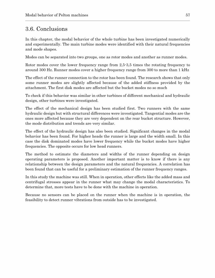
Modal behavior of Pelton machines 57
3.6. Conclusions
In this chapter, the modal behavior of the whole turbine has been investigated numerically
and experimentally. The main turbine modes were identified with their natural frequencies
and mode shapes.
Modes can be separated into two groups, one as rotor modes and another as runner modes.
Rotor modes cover the lower frequency range from 2,5-3,5 times the rotating frequency to
around 300 Hz. Runner modes cover a higher frequency range from 300 to more than 1 kHz
The effect of the runner connection to the rotor has been found. The research shows that only
some runner modes are slightly affected because of the added stiffness provided by the
attachment. The first disk modes are affected but the bucket modes no so much
To check if this behavior was similar in other turbines of different mechanical and hydraulic
design, other turbines were investigated.
The effect of the mechanical design has been studied first. Two runners with the same
hydraulic design but with structural differences were investigated. Tangential modes are the
ones more affected because they are very dependent on the rear bucket structure. However,
the mode distribution and trends are very similar.
The effect of the hydraulic design has also been studied. Significant changes in the modal
behavior has been found. For higher heads the runner is large and the width small. In this
case the disk dominated modes have lower frequency while the bucket modes have higher
frequencies. The opposite occurs for low head runners.
The method to estimate the diameters and widths of the runner depending on design
operating parameters is proposed. Another important matter is to know if there is any
relationship between the design parameters and the natural frequencies. A correlation has
been found that can be useful for a preliminary estimation of the runner frequency ranges.
In this study the machine was still. When in operation, other effects like the added mass and
centrifugal stresses appear in the runner what may change the modal characteristics. To
determine that, more tests have to be done with the machine in operation.
Because no sensors can be placed on the runner when the machine is in operation, the
feasibility to detect runner vibrations from outside has to be investigated.

58 3.6 Conclusions
Chapter 4 Transmissibility of runner
vibrations
During operation, the water jet impinges on the runner buckets generating large vibrations
and deformations on it. Damage in the runner depends on the amplitude and deformations
generated, therefore their monitoring is of paramount importance for the turbine
surveillance. Because sensors cannot be located directly on the runner, the feasibility to
detect runner vibrations in the monitoring positions has been addressed in this chapter.
First the propagation of the runner vibrations to the shaft and then to the bearing has been
investigated. Second the best monitoring positions to detect specific mode shapes have been
selected. The effects of bucket construction and location have been also investigated.
4.1. Experimental study of Arties machine
4.1.1. Equipment and procedure
To test the transmissibility of the bucket vibrations to the monitoring positions,
accelerometers were placed on the buckets (in the same way represented in Figure 3.13), on
the shaft and on both turbine bearings (as shown in Figure 3.1). The turbine runner was
accessible because the casing was removed. The accelerometers used were the same as in the
impact tests. The setup is shown in Figure 4.1.
The procedure consisted in impacting all the accessible buckets (from 21 to 11) in the axial,
tangential and radial direction. Also one bucket was impacted from underneath the wheel.

60 4.1 Experimental study of Arties machine
Figure 4.1. View of experimental setup
4.1.2. Transmissibility of vibrations
To investigate the transmission of vibrations from the buckets to the monitoring locations,
two series of tests were performed. Two accelerometers were placed on bucket 6 in the axial
and tangential directions and two other accelerometers were placed on the same line, one
vertically on the shaft between the bearing and the turbine, and another in the vertical
monitoring location A34. The first test consisted in performing axial impacts to the bucket
and calculating the FRF. In Figure 4.2 and Figure 4.3, the FRF’s of all these points have been
represented in the low frequency range (lower modes). As to be expected, the axial modes and
the radial modes are much more excited by the impingements than the tangential modes, as
seen in Figure 4.2. In Figure 4.3, it can be observed that the vibrations are transmitted to
the shaft and the bearing, even though the amplitude is smaller.
First point to see is that the transmission of the vibration from the bucket to the shaft and
from the shaft to the monitoring location varies with the type of mode. It can be seen that,
although the axial in-phase modes are the most excited in the bucket, the tangential and
axial counter-phase modes are comparatively better detected in the shaft and the bearing.
Thus, the transmission of these modes is better than for axial in-phase modes. In addition,
the transmission from shaft to bearing also varies with the mode, being the axial in-phase
modes the better transmitted.
450
[Hz]
500
[Hz]
550
[Hz]
600
[Hz]
650
[Hz]
700
[Hz]
0.4
0.8
1.2
1.6
2
2.4[(m/s^2)/N]
R2 (Magnitude)
R1 (Magnitude)
Figure 4.2. FRF of the response of axial (red) and tangential (blue) accelerometers placed on bucket 6 to axial
impacts on the bucket

Transmissibility of runner vibrations 61
450
[Hz]
500
[Hz]
550
[Hz]
600
[Hz]
650
[Hz]
700
[Hz]
4m
8m
12m
16m
20m
24m
28m
[(m/s^2)/N]
A34 (Magnitude)
E4V (Magnitude)
Figure 4.3. FRF of the response of A34 (blue) and E4V (green) accelerometers to axial impacts on the bucket
In Figure 4.4 and Figure 4.5, the same FRF’s are represented, but for the frequency range of
the higher modes (700-1300 Hz). The analysis of the higher natural frequencies shows that
the transmission of the radial modes is similar to the axial in-phase modes. Sometimes the
transmission is better in the bearing than in the shaft.
700
[Hz]
800
[Hz]
900
[Hz]
1k
[Hz]
1.1k
[Hz]
1.2k
[Hz]
0.4
0.8
1.2
1.6
2
2.4[(m/s^2)/N]
R2 (Magnitude)
R1 (Magnitude)
Figure 4.4. FRF of the response of axial (red) and tangential (blue) accelerometers placed on bucket 6 to axial
impacts on the bucket
700
[Hz]
800
[Hz]
900
[Hz]
1k
[Hz]
1.1k
[Hz]
1.2k
[Hz]
4m
8m
12m
16m
20m
24m
28m
[(m/s^2)/N]
A34 (Magnitude)
E4V (Magnitude)
Figure 4.5. FRF of the response of A34 (blue) and E4V (green) accelerometers to axial impacts on the bucket
The second test consisted in performing tangential impacts, with the accelerometers placed
tangentially in two different buckets. It is to be seen that there is a good transmission of the
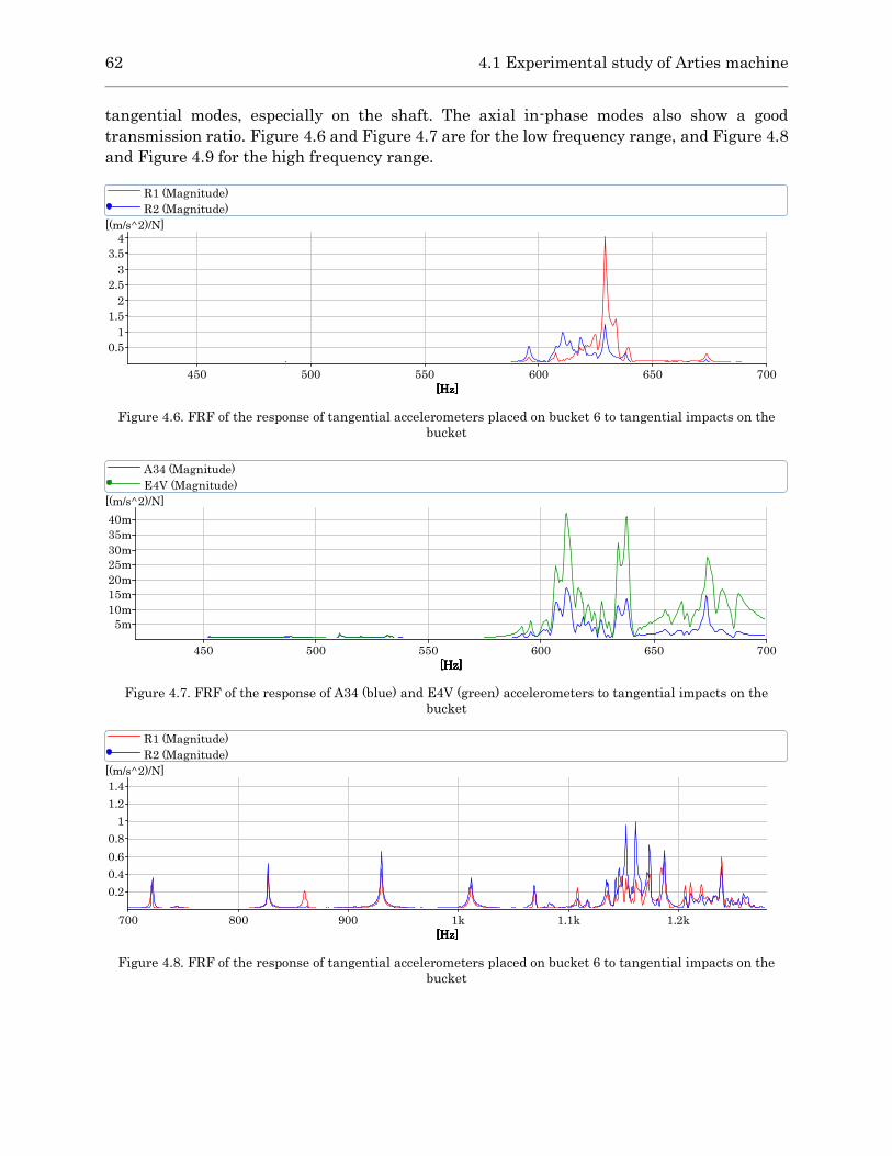
62 4.1 Experimental study of Arties machine
tangential modes, especially on the shaft. The axial in-phase modes also show a good
transmission ratio. Figure 4.6 and Figure 4.7 are for the low frequency range, and Figure 4.8
and Figure 4.9 for the high frequency range.
450
[Hz]
500
[Hz]
550
[Hz]
600
[Hz]
650
[Hz]
700
[Hz]
0.5
1
1.5
2
2.5
3
3.5
4[(m/s^2)/N]
R1 (Magnitude)
R2 (Magnitude)
Figure 4.6. FRF of the response of tangential accelerometers placed on bucket 6 to tangential impacts on the
bucket
450
[Hz]
500
[Hz]
550
[Hz]
600
[Hz]
650
[Hz]
700
[Hz]
5m
10m
15m
20m
25m
30m
35m
40m
[(m/s^2)/N]
A34 (Magnitude)
E4V (Magnitude)
Figure 4.7. FRF of the response of A34 (blue) and E4V (green) accelerometers to tangential impacts on the
bucket
700
[Hz]
800
[Hz]
900
[Hz]
1k
[Hz]
1.1k
[Hz]
1.2k
[Hz]
0.2
0.4
0.6
0.8
1
1.2
1.4
[(m/s^2)/N]
R1 (Magnitude)
R2 (Magnitude)
Figure 4.8. FRF of the response of tangential accelerometers placed on bucket 6 to tangential impacts on the
bucket

Transmissibility of runner vibrations 63
700
[Hz]
800
[Hz]
900
[Hz]
1k
[Hz]
1.1k
[Hz]
1.2k
[Hz]
5m
10m
15m
20m
25m
30m
35m
40m[(m/s^2)/N]
A34 (Magnitude)
E4V (Magnitude)
Figure 4.9. FRF of the response of A34 (blue) and E4V (green) accelerometers to tangential impacts on the
bucket
4.1.3. Detection from monitoring positions
In this part the transmission of the bucket vibration to the different bearing locations has
been studied. The objective is to determine which one is better to detect the different modes.
The procedure used was to perform impacts to the same bucket in the axial, tangential and
radial directions to excite the different types of modes and to evaluate which monitoring
locations (A31, A34, A35 and A38) are more suitable for mode detection. Since a horizontal
Pelton turbine is not a completely symmetric machine in terms of stiffness and transmission,
the tests were performed in three different buckets, which were located 90 degrees from each
other.
The results are showed in the following figures. The first test was performed in the bucket
21, which was located in the horizontal line of the turbine (same direction of the jet) and 180
degrees from the monitoring location A31. Three different frequency ranges have been
selected for the display of the results [0-550 Hz], [550-700 Hz] and [700-1300 Hz].
In Figure 4.10 and Figure 4.11, the FRF’s of the responses transmitted to the monitoring
locations A31, A34, A35 and A38 after impacting the bucket axially are represented,
respectively, in the range of 0-550 Hz. The lower frequencies, corresponding to the rotor
modes, show a better detection from the axial monitoring locations A35 and A38. For
example, the rotor modes at 163,5 Hz and 178,5 Hz are very well transmitted, especially to
A38, and the rotor mode at 50 Hz is better detected from A35. The runner axial modes with
less number of nodes (disk-dominated) are also better transmitted to the axial locations: the
1-ND, 2-ND and 3-ND axial in-phase modes are mostly seen from A35 and A38. Nevertheless,
the axial modes with more number of nodes (bucket-dominated modes), though they can be
detected from any position, have their best transmission ratio to the radial vertical
monitoring location A34.

64 4.1 Experimental study of Arties machine
0
[Hz]
100
[Hz]
200
[Hz]
300
[Hz]
400
[Hz]
500
[Hz]
1m
3m
5m
7m
9m
[(m/s^2)/N]
0
[Hz]
100
[Hz]
200
[Hz]
300
[Hz]
400
[Hz]
500
[Hz]
1m
3m
5m
7m
9m
[(m/s^2)/N]
Figure 4.10. FRF’s of the response from bearing position A31 (top) and A34 (bottom) to impacts on bucket 21 in
axial (red), tangential (blue) and radial (green) directions
0
[Hz]
100
[Hz]
200
[Hz]
300
[Hz]
400
[Hz]
500
[Hz]
1m
3m
5m
7m
9m
[(m/s^2)/N]
0
[Hz]
100
[Hz]
200
[Hz]
300
[Hz]
400
[Hz]
500
[Hz]
1m
3m
5m
7m
9m
[(m/s^2)/N]
Figure 4.11. FRF’s of the response from bearing positions A35 (top) and A38 (bottom) to impacts on bucket 21 in
axial (red), tangential (blue) and radial (green) directions
To check that the vibration measured from the sensors placed on the bearings is the same as
the vibration of the bucket, the coherence between both signals has been evaluated in the
range of the axial in-phase modes (420-550 Hz). According to the signals previously analyzed,
the vertical position A34 is more sensitive to these modes, so this has been analyzed in Figure
4.12. The same peaks are clearly discerned in both FFT signals, but with very different
amplitudes. The peak axial vibration of the bucket is around x200 times the peak vibration
transmitted to the bearings. It is worth noting that, even for the same type of modes, every
natural frequency has a different transmission ratio. Analyzing the coherence in the bottom
graph, it can be seen that this reaches the value of 1 in almost all the peaks. Therefore, it can
be confirmed that the vibration from both signals is of the same origin. The only exception is
the peak at the highest frequency, which has a very low coherence.

Transmissibility of runner vibrations 65
Figure 4.12. FFT and coherence between axial accelerometer on the bucket and vertical position A34
The transmission of the axial modes to the monitoring positions has been evaluated
calculating the RMS acceleration values of the frequency band [420-550 Hz] from all the
positions (see Table 4.1). The ratio between the vibration of the bearing positions with respect
to the axial bucket acceleration has been calculated. As expected, the accelerometer on the
axial position has the highest vibration levels. The percentage of energy sensed by the
accelerometers on the bearings is about 0,3% the value of AA. The best position for this modes
is the vertical radial.
Table 4.1. Axial RMS acceleration values between bucket 21 and monitoring positions
Location Acceleration RMS [m/s²] Ratio [%]
Bucket AA 29,89
Bucket TA 1,111
Bucket RA 3,24
A31 0,03109 0,1040
A34 0,09449 0,3161
A35 0,04045 0,1353
A38 0,04328 0,1448
In Figure 4.13 and Figure 4.14, the FRF’s are represented in the range 550-700 Hz. The
tangential modes are excited by the impacts in the tangential and radial directions and have
a similar transmission in all the monitoring points. It can be said, though, that A38 receives
most part of the vibration, especially for the mode at 602,5 Hz, which corresponds to the
natural frequency of the tangential mode of bucket 21. For the case of the axial counter-phase

66 4.1 Experimental study of Arties machine
mode, only the frequency of the impacted bucket is excited, and thus received in the
monitoring positions. The accelerometer in the radial horizontal position A31 is the one that
best detects the vibration of the bucket.
550
[Hz]
600
[Hz]
650
[Hz]
700
[Hz]
10m
20m
30m
40m
50m
60m
[(m/s^2)/N]
550
[Hz]
600
[Hz]
650
[Hz]
700
[Hz]
10m20m30m40m50m60m
[(m/s^2)/N]
Figure 4.13. FRF’s of the response from bearing position A31 (top) and A34 (bottom) to impacts on bucket 21 in
axial (red), tangential (blue) and radial (green) directions
550
[Hz]
600
[Hz]
650
[Hz]
700
[Hz]
010m20m30m40m50m60m
[(m/s^2)/N]
550
[Hz]
600
[Hz]
650
[Hz]
700
[Hz]
10m20m30m40m50m60m
[(m/s^2)/N]
Figure 4.14. FRF’s of the response from bearing position A35 (top) and A38 (bottom) to impacts on bucket 21 in
axial (red), tangential (blue) and radial (green) directions
The coherence between the signal of the accelerometer installed tangentially on bucket 21
and the bearing location A38 is represented in Figure 4.15. As seen in the axial impacts, the
same peaks can be found in both signals, with good coherence for most of them, but the
relative magnitudes vary.

Transmissibility of runner vibrations 67
Figure 4.15. FFT and coherence between tangential accelerometer on the bucket and position A38
The range of the tangential [590-620 Hz] and torsional modes [620-635 Hz] has been
evaluated in Table 4.2. At first sight, it is noticeable that for both kinds of modes, the
accelerometer in radial direction RA vibrates more than the others. The tangential modes
have very good transmission, and especially to the axial position A38.
Table 4.2. Tangential RMS acceleration values between bucket 21 and monitoring positions
Location Acceleration RMS
[m/s²]
Ratio [%] Acceleration RMS
[m/s²]
Ratio [%]
Bucket AA 3,898 - 2,923 -
Bucket TA 3,154 - 1,925 -
Bucket RA 7,737 - 6,477 -
A31 0,0865 2,743 0,01706 0,886
A34 0,111 3,519 0,02157 1,121
A35 0,1007 3,193 0,0244 1,268
A38 0,1854 5,878 0,03035 1,577
The rim modes are located in the range [640-690 Hz], for the RMS acceleration values have
been calculated and listed in Table 4.3. The transmission is not as good as in the other cases,
although the reference value is the vibration from the axial accelerometer AA, which is very
high here. In this type of mode, the vibration is located almost completely in the bucket’s rim,
where the accelerometer is placed, so the sensitivity is very high. The best transmission ratio
is from A35, but the difference with the other locations is not high.

68 4.1 Experimental study of Arties machine
Table 4.3. Axial RMS acceleration values between bucket 21 and monitoring positions
Location Acceleration RMS [m/s²] Ratio [%]
Bucket AA 114,2 -
Bucket TA 9,612 -
Bucket RA 45 -
A31 0,2171 0,190
A34 0,1664 0,146
A35 0,2443 0,214
A38 0,2235 0,196
The results for the last range of frequencies 700-1300 Hz are showed in Figure 4.16 and
Figure 4.17. The radial counter-phase modes are mostly excited by the tangential impacts
and their transmission is similar to all the monitoring locations. However, the radial in-phase
modes (1120-1200 Hz) and the radial-axial counter-phase modes (1200-1300 Hz), which are
mostly excited by the radial impacts, have clearly the best transmission to the axial vertical
monitoring location A38.
700
[Hz]
800
[Hz]
900
[Hz]
1k
[Hz]
1.1k
[Hz]
1.2k
[Hz]
1.3k
[Hz]
40m
0.12
0.2
0.28
0.36
[(m/s^2)/N]
700
[Hz]
800
[Hz]
900
[Hz]
1k
[Hz]
1.1k
[Hz]
1.2k
[Hz]
1.3k
[Hz]
40m
0.12
0.2
0.28
0.36
[(m/s^2)/N]
Figure 4.16. FRF of the response of bearing positions A31 (top) and A34 (bottom) to impacts in bucket 21 in
axial (red), tangential (blue) and radial (green) directions

Transmissibility of runner vibrations 69
700
[Hz]
800
[Hz]
900
[Hz]
1k
[Hz]
1.1k
[Hz]
1.2k
[Hz]
1.3k
[Hz]
40m
0.12
0.2
0.28
0.36
[(m/s^2)/N]
700
[Hz]
800
[Hz]
900
[Hz]
1k
[Hz]
1.1k
[Hz]
1.2k
[Hz]
1.3k
[Hz]
40m
0.12
0.2
0.28
0.36
[(m/s^2)/N]
Figure 4.17. FRF of the response of bearing positions A35 (top) and A38 (bottom) to impacts in bucket 21 in
axial (red), tangential (blue) and radial (green) directions
The RMS values of the radial modes (Table 4.4) show that, as seen in the plots, the axial
location A38 is by far the most sensitive. The ratio has been calculated with respect to the
radial accelerometer RA, which captures best the radial motion of the bucket.
Table 4.4. Radial RMS acceleration values between bucket 21 and monitoring positions
Location Acceleration RMS [m/s²] Ratio [%]
Bucket AA 33,06 -
Bucket TA 10,82 -
Bucket RA 58,8 -
A31 0,3292 0,5599
A34 0,09604 0,1633
A35 0,1877 0,3192
A38 0,9662 1,6432
Another series of tests were performed but impacting another bucket (bucket 16) which was
located in the vertical plane of the turbine, which is the same as the monitoring position A34.
The results showed in the following pictures were obtained by performing axial, tangential
and radial impacts to bucket 16. In Figure 4.18, the resulting FRF’s are showed in the range
0-550 Hz. As seen in the previous tests, the frequencies corresponding to the rotor modes of
the turbines are better detected from the axial monitoring positions. The choice between the
vertical and the horizontal positions depends on the mode. The axial bucket-dominated
runner modes also have the best transmission to the monitoring location A34.

70 4.1 Experimental study of Arties machine
In Figure 4.19, the FRF’s in the range between 550 and 700 Hz are represented. The range
of tangential modes is similarly detected by the four accelerometers, except the tangential
mode corresponding to the bucket excited, which clearly outstands in the axial vertical sensor
A38. When it comes to the axial counter-phase mode excited by the impact, in this case at
649 Hz since we are impacting a different bucket, there is a slight better detection from A31.
Thus, the features of the transmission are the same as for the previous impacts to bucket 21.
Finally, the range between 700 and 1300 Hz is displayed in Figure 4.20. It is once again clear
that radial in-phase and radial-axial counter-phase modes are by far best detected from
position A38, unlike the radial counter-phase modes, which shows similar transmission to all
four points.
0
[Hz]
100
[Hz]
200
[Hz]
300
[Hz]
400
[Hz]
500
[Hz]
01m2m3m4m5m6m7m8m9m
[(m/s^2)/N]
0
[Hz]
100
[Hz]
200
[Hz]
300
[Hz]
400
[Hz]
500
[Hz]
1m2m3m4m5m6m7m8m9m
[(m/s^2)/N]
Figure 4.18. FRF’s of the response from bearing position A34 (top) and A38 (bottom) to impacts on bucket 16 in
axial (red), tangential (blue) and radial (green) directions
The transmission has been calculated in the same way as the impact in bucket 21. This time,
the RMS acceleration value of the axial frequency band is evaluated with respect to the
accelerometer in bucket 16. The response of the bucket is very similar to the impacts in
bucket 21, as well as the transmission ratios. Again, position A34 is proved to be the most
sensitive one.
Table 4.5. Axial RMS acceleration values between bucket 16 and monitoring positions
Location Acceleration RMS [m/s²] Ratio [%]
Bucket 16AA 29,32 -
A31 0,04649 0,1586
A34 0,1129 0,3851
A35 0,04657 0,1588
A38 0,04638 0,1582
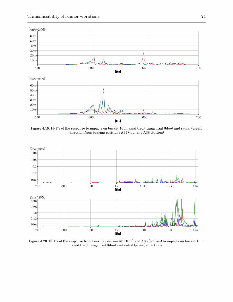
Transmissibility of runner vibrations 71
550
[Hz]
600
[Hz]
650
[Hz]
700
[Hz]
10m
20m
30m
40m
50m
60m
[(m/s^2)/N]
550
[Hz]
600
[Hz]
650
[Hz]
700
[Hz]
10m
20m
30m
40m
50m
60m
[(m/s^2)/N]
Figure 4.19. FRF’s of the response to impacts on bucket 16 in axial (red), tangential (blue) and radial (green)
direction from bearing positions A31 (top) and A38 (bottom)
700
[Hz]
800
[Hz]
900
[Hz]
1k
[Hz]
1.1k
[Hz]
1.2k
[Hz]
1.3k
[Hz]
40m
0.12
0.2
0.28
0.36
[(m/s^2)/N]
700
[Hz]
800
[Hz]
900
[Hz]
1k
[Hz]
1.1k
[Hz]
1.2k
[Hz]
1.3k
[Hz]
40m
0.12
0.2
0.28
0.36
[(m/s^2)/N]
Figure 4.20. FRF’s of the response from bearing position A31 (top) and A38 (bottom) to impacts on bucket 16 in
axial (red), tangential (blue) and radial (green) directions

72 4.1 Experimental study of Arties machine
Lastly, a test similar to the previous ones was performed to the bucket near the location
where the jet impacts the runner (bucket 6). This time, accelerometers were placed on
positions A31 and A34. In Figure 4.21, the FRF’s obtained are showed in the range 0-550 Hz.
It can be seen that axial bucket-dominated modes are better transmitted to A34, like observed
in the previous tests.
0
[Hz]
100
[Hz]
200
[Hz]
300
[Hz]
400
[Hz]
500
[Hz]
1m2m3m4m5m6m7m8m9m
[(m/s^2)/N]
0
[Hz]
100
[Hz]
200
[Hz]
300
[Hz]
400
[Hz]
500
[Hz]
1m2m3m4m5m6m7m8m9m
[(m/s^2)/N]
Figure 4.21. FRF of the response of bearing positions A31 (top) and A34 (bottom) to impacts in bucket 6 in axial
(red) and tangential (blue) directions
Figure 4.22. Coherence between bearing acc. A34 and bucket 6 acc.

Transmissibility of runner vibrations 73
Again, in Table 4.6 it is proved that the vertical position has the best sensitivity to the axial
modes.
Table 4.6. Axial RMS acceleration values between bucket 6 and monitoring positions
Location Acceleration RMS [m/s²] Ratio[%]
R4 axial 8,031 -
R2 radial 7,204 -
A31 0,01457 0,1814
A34 0,04395 0,5473
E4V 0,05564 0,6928
The FRF’s from A31 and A34 are showed in the range 550-700 Hz in Figure 4.23. Tangential
modes have similar transmissibility between both locations. However, the axial counter-
phase mode for this bucket at 674 Hz have almost twice better transmission in position A31
than A34. This confirms the behavior identified in the previous tests.
550
[Hz]
600
[Hz]
650
[Hz]
700
[Hz]
10m
20m
30m
40m
50m
60m
[(m/s^2)/N]
550
[Hz]
600
[Hz]
650
[Hz]
700
[Hz]
10m
20m
30m
40m
50m
60m
[(m/s^2)/N]
Figure 4.23. FRF of the response of bearing positions A31 (top) and A34 (bottom) to impacts in bucket 6 in axial
(red) and tangential (blue) directions
All the tests have been used to determine which locations are the most suitable to identify
the turbine modes. In general terms, the vertical positions provide a better transmission ratio
than horizontal positions. This can be associated to the fact that the shaft has a closer contact
to the bearing ring in the vertical positions due to the effect of the weight load.
To quantify the transmission, the energy bands corresponding to the different bucket modes
have been filtered and calculated. For almost all bands the best detection position is the
vertical location A34.

74 4.1 Experimental study of Arties machine
4.1.4. Scattering of runner frequencies
To check the scattering of the natural frequencies of each bucket, transmission tests for all
the buckets were carried out. The results are indicated in Figure 4.24 and Figure 4.25, where
the tangential and axial counter-phase frequencies measured from the bearings after
impacting all the accessible buckets have been represented together. It can be seen that the
rim modes are more local than tangential modes, since every bucket has its own natural
frequency, which doesn’t affect the other buckets. The scattering is quite important in both
cases. A difference of about 7% (~50 Hz) can be found in these modes due to mechanical
inaccuracies and/or different erosion between buckets. It is also worth noting that the
transmission is different for every frequency.
580
[Hz]
590
[Hz]
600
[Hz]
610
[Hz]
620
[Hz]
630
[Hz]
640
[Hz]
5m
10m
15m
20m
25m
30m
35m
40m
[(m/s^2)/N]
Figure 4.24. Frequencies of the tangential mode for different buckets
630
[Hz]
640
[Hz]
650
[Hz]
660
[Hz]
670
[Hz]
680
[Hz]
690
[Hz]
700
[Hz]
10m
20m
30m
40m
50m
60m
70m
80m
90m
[(m/s^2)/N]
Figure 4.25. Frequencies of the rim mode for different buckets

Transmissibility of runner vibrations 75
4.2. Experimental study of Moncabril machine
The transmissibility of vibrations between the runner and the monitoring locations has been
also studied for the Pelton turbine of Moncabril power plant. The same setup used for the
impact tests (Figure 3.17) was used to study the transmissibility of this machine.
4.2.1. Choice of best monitoring positions
In this case only the turbine bearing has been studied, due to its proximity to the runner.
Two accelerometers were placed in the horizontal and vertical direction of bearing 1, and
axial and tangential impacts were performed to the buckets which were accessible from
underneath the turbine. In Figure 4.26, it can be seen that the rotor modes are detected from
both directions, but the horizontal position has a slight better transmission.
0
[Hz]
40
[Hz]
80
[Hz]
120
[Hz]
160
[Hz]
200
[Hz]
240
[Hz]
500u1m
1.5m2m
2.5m3m
3.5m4m
4.5m
[(m/s^2)/N]
0
[Hz]
40
[Hz]
80
[Hz]
120
[Hz]
160
[Hz]
200
[Hz]
240
[Hz]
500u1m
1.5m2m
2.5m3m
3.5m
4m4.5m
[(m/s^2)/N]
Figure 4.26. FRF’s of the response from bearing positions A13 (top) and A14 (bottom) to impacts in axial (red)
and tangential (blue) directions
The axial modes are excited by the axial impacts and, as seen in the previous section, are
better detected from the vertical monitoring position A14. It can be seen that the
transmission is better for high modes.
The vertical position also shows the better detection of the tangential and the axial counter-
phase modes.
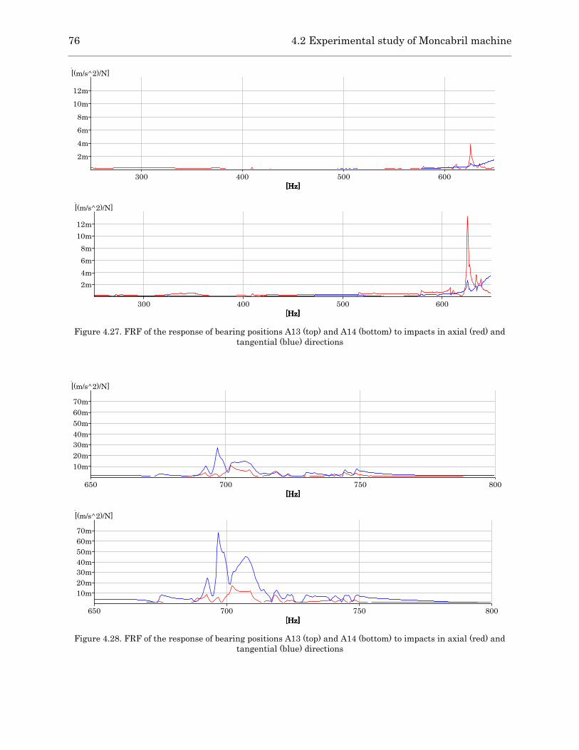
76 4.2 Experimental study of Moncabril machine
300
[Hz]
400
[Hz]
500
[Hz]
600
[Hz]
2m
4m
6m
8m
10m
12m
[(m/s^2)/N]
300
[Hz]
400
[Hz]
500
[Hz]
600
[Hz]
2m
4m
6m
8m
10m
12m
[(m/s^2)/N]
Figure 4.27. FRF of the response of bearing positions A13 (top) and A14 (bottom) to impacts in axial (red) and
tangential (blue) directions
650
[Hz]
700
[Hz]
750
[Hz]
800
[Hz]
10m
20m
30m
40m
50m
60m
70m
[(m/s^2)/N]
650
[Hz]
700
[Hz]
750
[Hz]
800
[Hz]
10m
20m
30m
40m
50m
60m
70m
[(m/s^2)/N]
Figure 4.28. FRF of the response of bearing positions A13 (top) and A14 (bottom) to impacts in axial (red) and
tangential (blue) directions
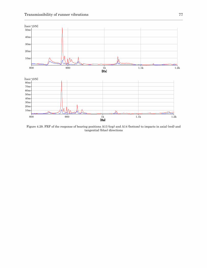
Transmissibility of runner vibrations 77
800
[Hz]
900
[Hz]
1k
[Hz]
1.1k
[Hz]
1.2k
[Hz]
10m
20m
30m
40m
50m
[(m/s^2)/N]
800
[Hz]
900
[Hz]
1k
[Hz]
1.1k
[Hz]
1.2k
[Hz]
10m
20m
30m
40m
50m
60m
70m
80m
[(m/s^2)/N]
Figure 4.29. FRF of the response of bearing positions A13 (top) and A14 (bottom) to impacts in axial (red) and
tangential (blue) directions

78 4.3 Conclusions
4.3. Conclusions
The propagation of vibrations from runner to bearings in two different turbines was
investigated. The experimental investigation shows that all the runner vibrations are
transmitted and detected on the bearing. High coherence values are found between runner
and bearing vibrations. Anyway, the amplitudes seen in the bearing are much smaller than
the amplitudes in the runner.
The propagation of the runner natural frequencies to each monitoring position depends on
the mode shapes. The tangential modes are better propagated than axial modes
In general, tangential modes are better propagated than axial modes
In general terms, vertical positions have better transmissibility than horizontal positions.
The only exception are the axial counter-phase modes, which are better transmitted to
horizontal positions.
In addition, rotor modes and disk-dominated modes are generally better detected from axial
bearing locations, while bucket dominated modes transmit their vibration better to the radial
positions.
The best monitoring positions for the machines studied are the vertical position in the turbine
bearing.
A detailed analysis shows that there are small differences between the natural frequencies
of each bucket.
So far, the turbine has been studied still. In operation some effects like the centrifugal forces
and the added mass, can modify the natural frequencies. Moreover, the modes excited during
operation have to be determined.
For that and with the knowledge obtained with the previous studies, the dynamic behavior
of a Pelton turbine in operation has been performed and presented in the next chapter.

Chapter 5 Dynamic analysis of Pelton
turbines
In the previous chapter, it was proved that the vibration of the runner buckets can be detected
from the bearings, and that the transmission depends on the bucket mode and on the
monitoring location and direction. However, the dynamics of a Pelton turbine in operation
are more complex, due to the effect of the rotational forces, the electrical excitation and the
water jets.
In this chapter, the dynamic behavior of two different Pelton turbines, Arties and Moncabril,
has been investigated at different operating conditions. The first analysis consists in
identifying the modes excited during the start-up transient of the turbine. Second, the
vibration of the machine under steady operating conditions has been analyzed with the
purpose of identifying which modes are excited in normal operating conditions. Finally, the
frequency bands where the different runner modes are found and their RMS vibration values
have been determined.
5.1. Dynamic behavior of Arties PT
5.1.1. On-site measurements
The instrumentation used for the measurements in the power plant of Arties consisted of
nine accelerometers and one strain gauge. The sensors were disposed as shown on the sketch
in Figure 5.1. Eight accelerometers were placed on both bearings in the same positions as the
impact tests (A11, A14, A15, and A18 on turbine bearing one, and A31, A34, A35 and A38 on
turbine bearing two).

80 5.1 Dynamic behavior of Arties PT
In addition, an onboard system with one accelerometer and one strain gauge was installed
on the shaft between turbine 2 and bearing 2 (Figure 5.2 left). A strain gauge is a sensor
whose resistance varies with the applied force. The one used for the tests was a pre-wired
gauge HBM K-CDY4-0030-1-350-3-005 with a grid length of 3 mm, a nominal resistance of
350 Ohm and cable length of 0,5 m.
Figure 5.1. Sketch of the position of the sensors during on-site measurements
Figure 5.2. On the left, onboard system installed on the shaft and on the right, horizontal accelerometers placed
on the turbine bearing
The test performed consisted in recording the vibration of the machine during a whole
operating cycle, from the machine being still to operating at maximum load. The operating
parameters of the turbine at every instant were known thanks to the software SCADA
(Supervisory Control and Data Acquisition), which is used by the power plant operators to
control and monitor the operation of the turbine. Figure 5.3 shows a screenshot of the
program when the turbine is operating at minimum load. Among other parameters, one can
see the rotational speed, the opening degree of the nozzles and the overall vibration levels.
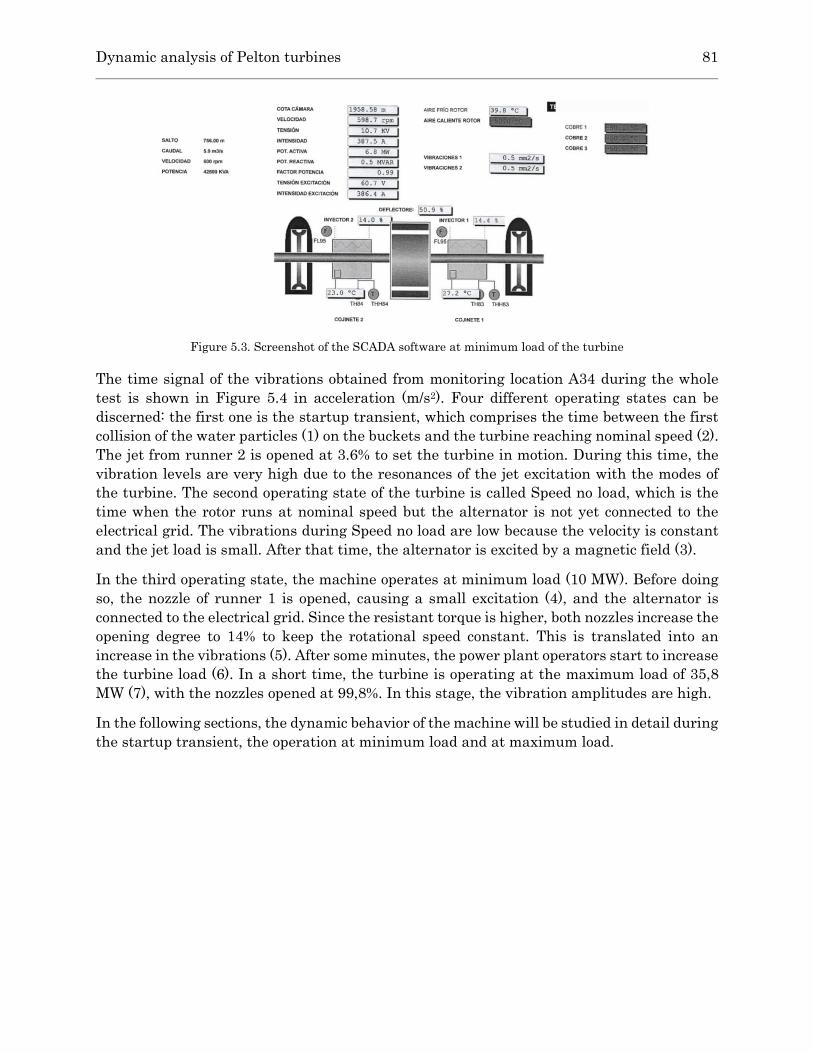
Dynamic analysis of Pelton turbines 81
Figure 5.3. Screenshot of the SCADA software at minimum load of the turbine
The time signal of the vibrations obtained from monitoring location A34 during the whole
test is shown in Figure 5.4 in acceleration (m/s2). Four different operating states can be
discerned: the first one is the startup transient, which comprises the time between the first
collision of the water particles (1) on the buckets and the turbine reaching nominal speed (2).
The jet from runner 2 is opened at 3.6% to set the turbine in motion. During this time, the
vibration levels are very high due to the resonances of the jet excitation with the modes of
the turbine. The second operating state of the turbine is called Speed no load, which is the
time when the rotor runs at nominal speed but the alternator is not yet connected to the
electrical grid. The vibrations during Speed no load are low because the velocity is constant
and the jet load is small. After that time, the alternator is excited by a magnetic field (3).
In the third operating state, the machine operates at minimum load (10 MW). Before doing
so, the nozzle of runner 1 is opened, causing a small excitation (4), and the alternator is
connected to the electrical grid. Since the resistant torque is higher, both nozzles increase the
opening degree to 14% to keep the rotational speed constant. This is translated into an
increase in the vibrations (5). After some minutes, the power plant operators start to increase
the turbine load (6). In a short time, the turbine is operating at the maximum load of 35,8
MW (7), with the nozzles opened at 99,8%. In this stage, the vibration amplitudes are high.
In the following sections, the dynamic behavior of the machine will be studied in detail during
the startup transient, the operation at minimum load and at maximum load.
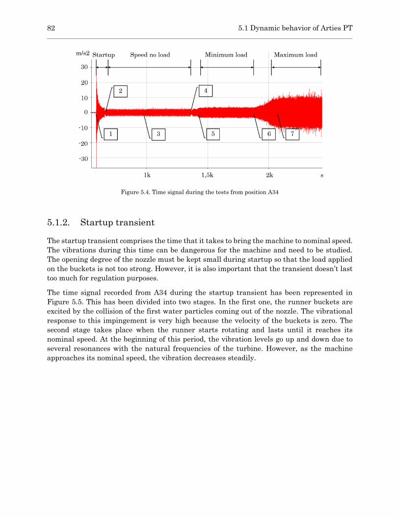
82 5.1 Dynamic behavior of Arties PT
Figure 5.4. Time signal during the tests from position A34
5.1.2. Startup transient
The startup transient comprises the time that it takes to bring the machine to nominal speed.
The vibrations during this time can be dangerous for the machine and need to be studied.
The opening degree of the nozzle must be kept small during startup so that the load applied
on the buckets is not too strong. However, it is also important that the transient doesn’t last
too much for regulation purposes.
The time signal recorded from A34 during the startup transient has been represented in
Figure 5.5. This has been divided into two stages. In the first one, the runner buckets are
excited by the collision of the first water particles coming out of the nozzle. The vibrational
response to this impingement is very high because the velocity of the buckets is zero. The
second stage takes place when the runner starts rotating and lasts until it reaches its
nominal speed. At the beginning of this period, the vibration levels go up and down due to
several resonances with the natural frequencies of the turbine. However, as the machine
approaches its nominal speed, the vibration decreases steadily.

Dynamic analysis of Pelton turbines 83
Figure 5.5. Time signal during startup transient from A34
The time signal recorded from position A34 has been represented in Figure 5.6 in the
frequency domain. This representation is known as waterfall and shows the change in the
vibration spectrum over time. In the figure, the first impact and the speedup of the turbine
can be clearly identified. Before the runner starts rotating, different frequency bands are
excited by the first collision of the jet. These correspond to the modes of the turbine, which
can be divided into rotor modes (0-400 Hz) and runner modes (>400 Hz). After that, the
runner starts accelerating (Speed-up). The rotation of the machine and the force of the jet are
clearly detected at every instant. The frequency of rotation 𝑓𝑓 can be expressed as
𝑓𝑓 = 𝑁 60⁄ Eq. 5.1
Where 𝑁 is the rotational speed in min-1. At nominal speed (600 min-1) the 𝑓𝑓 is 10 Hz. The
bucket passing frequency 𝑓𝑏 determines the rate at which the jet impinges the runner buckets
and can be written as
𝑓𝑏 = 𝑧𝑏𝑓𝑓 Eq. 5.2
Where 𝑧𝑏 is the number of buckets. At nominal speed, the bucket passing frequency is 220
Hz. During the speed-up, the turbine enters into resonance with the turbine modes every
time the 𝑓𝑏 is the same as a natural frequency of the structure (Campbell diagram). It is
worth noting that the vibration is higher at the beginning of the speed-up than at the end
because the velocity of the runner is still much lower than nominal speed, and this causes
the jet to impinge the buckets with very high velocity. After the machine has reached its
nominal speed, the vibration levels diminish considerably and mainly the 𝑓𝑓, the 𝑓𝑏 and their
harmonics are noticeable.
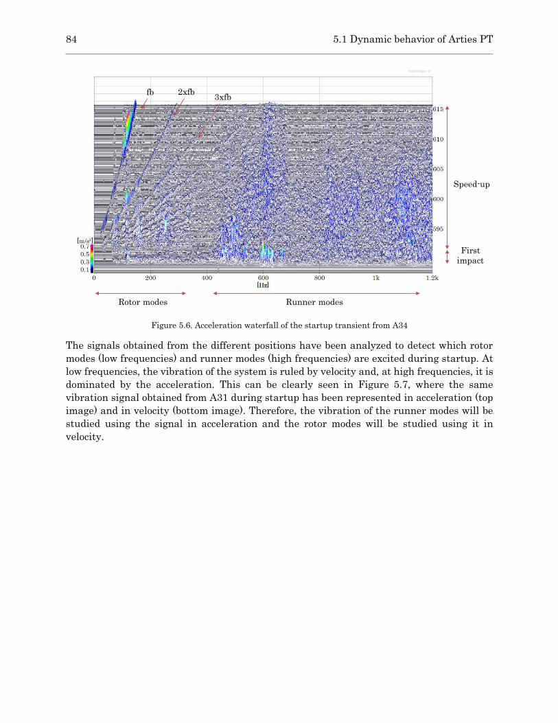
84 5.1 Dynamic behavior of Arties PT
Figure 5.6. Acceleration waterfall of the startup transient from A34
The signals obtained from the different positions have been analyzed to detect which rotor
modes (low frequencies) and runner modes (high frequencies) are excited during startup. At
low frequencies, the vibration of the system is ruled by velocity and, at high frequencies, it is
dominated by the acceleration. This can be clearly seen in Figure 5.7, where the same
vibration signal obtained from A31 during startup has been represented in acceleration (top
image) and in velocity (bottom image). Therefore, the vibration of the runner modes will be
studied using the signal in acceleration and the rotor modes will be studied using it in
velocity.
Rotor modes Runner modes
First
impact
Speed-up
fb 2xfb3xfb

Dynamic analysis of Pelton turbines 85
Figure 5.7. Waterfall of the startup transient from A31 in acceleration m/s2 (top) and velocity mm/s (bottom)
The collision of the first water particles coming out of the nozzle induces a large vibration on
the turbine. This is attributed to the fact that with the runner still, the jet enters the buckets
at a relative velocity that doubles that from steady operation. This aggravates the effects of

86 5.1 Dynamic behavior of Arties PT
the transient inside the buckets and makes it more prone to excite the natural modes of the
runner. In addition, the water can also show some deviations with respect to the optimal jet
shape, due to the small transitory that takes place inside the nozzle after the displacement
of the needle. In order to minimize the harmful effects on the structure, the opening degree
of the nozzle is kept small during startup.
The study of the initial jet impact is of interest due to its similarity with the impact tests.
The runner is still not affected by rotational or electrical forces, and, moreover, only one or
two buckets are impinged, for the vibration is not mixed between all the buckets like in steady
operation. The dynamic behavior of the turbine during the initial instant is thus less complex
than for the rest of the operating cycle, and the characteristics of the jet and the
transmissibility of the vibrations can be analyzed more accurately.
Observing Figure 5.7 top, it can be seen that the runner modes are more excited than the
rotor modes in the initial seconds of the transient. These require much less energy to oscillate,
for the mass displaced is much lower. Since the excitation of the rotor modes is more
significant during the speedup of the turbine, only the runner modes will be studied in the
initial impact. These will be identified from the different monitoring locations and the results
will be compared to the impact tests performed on the still machine. In addition, the
transmissibility of the vibrations to the shaft will also be checked with the measurements
from the on-board system.
The vibration recorded from the accelerometer in position A31 is shown in Figure 5.8.
According to the information obtained in the impact tests, four different types of runner
modes are found between 500 and 700 Hz: axial modes, tangential modes (in phase and in
counter-phase) and axial counter-phase modes. The frequency ranges corresponding to each
mode type have been delimited in red to be compared with the peaks detected at the start of
the transient. Observing the figure, it is clear that the frequencies excited by the initial jet
collision are very similar to the ones obtained in the impact tests. The most outstanding
frequencies correspond to the tangential and the axial counter-phase modes, which is to be
expected, for the jet impinges the buckets tangentially and the water is deflected by the
buckets’ rim. The most prominent peak is located at 668 Hz in the range of the axial counter-
phase modes, which corresponds to the natural frequency of the impacted bucket.
The vibration in the axial frequencies is low comparatively to other modes. However, it should
be remembered that, as seen in Chapter 4, their transmission to the bearings is lower, what
means that the vibration of the runner is higher.
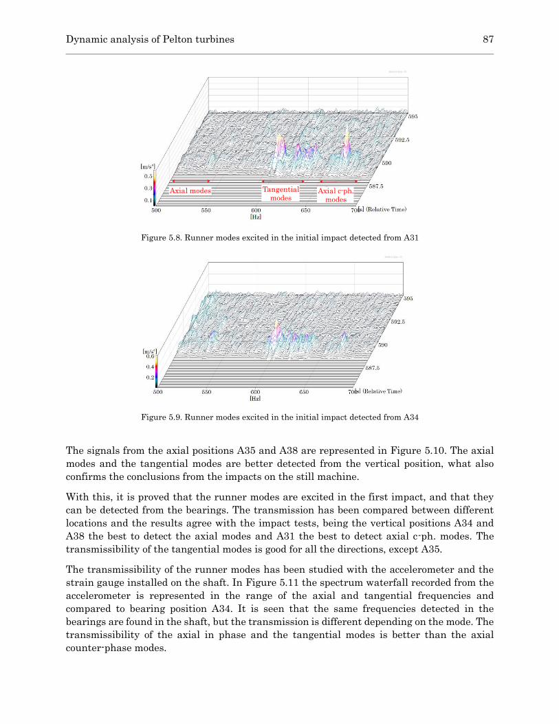
Dynamic analysis of Pelton turbines 87
Figure 5.8. Runner modes excited in the initial impact detected from A31
Figure 5.9. Runner modes excited in the initial impact detected from A34
The signals from the axial positions A35 and A38 are represented in Figure 5.10. The axial
modes and the tangential modes are better detected from the vertical position, what also
confirms the conclusions from the impacts on the still machine.
With this, it is proved that the runner modes are excited in the first impact, and that they
can be detected from the bearings. The transmission has been compared between different
locations and the results agree with the impact tests, being the vertical positions A34 and
A38 the best to detect the axial modes and A31 the best to detect axial c-ph. modes. The
transmissibility of the tangential modes is good for all the directions, except A35.
The transmissibility of the runner modes has been studied with the accelerometer and the
strain gauge installed on the shaft. In Figure 5.11 the spectrum waterfall recorded from the
accelerometer is represented in the range of the axial and tangential frequencies and
compared to bearing position A34. It is seen that the same frequencies detected in the
bearings are found in the shaft, but the transmission is different depending on the mode. The
transmissibility of the axial in phase and the tangential modes is better than the axial
counter-phase modes.
Axial modes Tangential
modesAxial c-ph.
modes
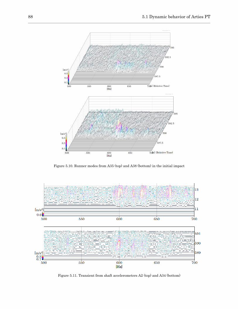
88 5.1 Dynamic behavior of Arties PT
Figure 5.10. Runner modes from A35 (top) and A38 (bottom) in the initial impact
Figure 5.11. Transient from shaft accelerometers A2 (top) and A34 (bottom)

Dynamic analysis of Pelton turbines 89
The signal obtained from the strain gauge has also been analyzed and it has been proved that
the runner modes also perform a strain on the shaft. The same range of frequencies is
represented in Figure 5.12 from the strain gauge and the shaft accelerometer. The tangential
modes are well detected by the gauge and have good coherence with respect to the
accelerometer. The axial in-phase and counter-phase perform a lower strain on the shaft, but
also can be distinguished.
Figure 5.12. Spectra waterfall from strain gauge (bottom), from shaft accelerometer (middle) and coherence
between both signals (top)
After the first impact, the turbine starts to increase its velocity and the water jet is converted
into a periodic load applied to all of the buckets. The structure is then affected by the
centrifugal forces, which increase its stiffness and vary its natural frequencies. With the
increment of the frequency of rotation, the load of the jet enters into resonance with the
natural frequencies of the turbine, especially with modes of the rotor, which are found below
the 300 Hz. To understand the effect of the new operating conditions on the dynamic behavior
of the machine, the speed-up has been divided into two periods. The first one covers the
behavior of the machine at the beginning of the speed-up, when the velocity of the runner is
low and the vibration is high due to resonances with rotor and runner modes. The second
period comprises the end of the startup, when the runner is near its nominal speed. The
vibrations are then considerably lower, and mainly resonances with the lowest harmonics of
the excitation take place.

90 5.1 Dynamic behavior of Arties PT
In the initial stage of the speed up, first the rotor modes have been studied. The frequencies
excited between 0 and 250 Hz detected from A38 are shown in Figure 5.13. Many peaks can
be observed due to the resonance of the turbine modes with the excitation frequency 𝑓𝑏 and
its harmonics. Four frequency bands are identified, which correspond to different bending
modes of the rotor. Some excitations haven’t been identified in the impact tests, which can
be due to resonances with the system frequencies.
Figure 5.13. Startup from position A38
The strain gauge cannot detect as well the bending modes of the rotor as the accelerometers
on the bearings, but provides a clear evidence of the excitation of the torsional modes at 54
Hz, what is difficult to find for any other sensor.
Figure 5.14. Torsional rotor mode detected with the strain gage

Dynamic analysis of Pelton turbines 91
The excitation of the runner modes during the speedup is analyzed in this section. The range
of frequencies 500-700 Hz has been analyzed from position A34, just after the first collision
of the jet (Figure 5.15) and at the end of the transient, when the machine is almost rotating
at nominal speed (Figure 5.16). In both figures, the ranges of the axial in phase, tangential
(phase and counter-phase) and the axial counter-phase modes have been delimited after the
results obtained in the impact tests. In the beginning of the speedup many peaks can be
discerned, due to the mixed vibration from different buckets. As seen in Chapter 4, each
bucket has its own natural frequency, which is different from the others. These still have still
very low velocity and the jet excitation has an important random component. Just after the
first impact, the range of the axial modes is the most excited by the jet forces. As the runner
increases its velocity, the main excitation forces increase their frequency, exciting the
tangential modes between 600 and 605 seconds. With this, the main frequency ranges can be
discerned and compared to the results for the still machine. Comparing both, it is seen that
the natural frequencies are very similar.
Figure 5.15. Axial and tangential modes from positon A34 at the start of the speed-up
At the end of the transient, the velocity of the runner is adjusted to meet its nominal speed
(600 min-1). Due to the resonance of the runner modes with the harmonics of the 𝑓𝑓 and 𝑓𝑏,
different peaks stick out. In the range of the axial modes the most excited frequencies
correspond to the bucket-dominated modes. It can be seen that some of the frequencies have
increased with respect to the still machine, which is due to the higher stiffness of the
structure caused by the rotational velocity. The tangential modes aren’t as much excited as
the axial modes. Some frequencies in the range of the axial counter-phase modes are excited
by the 3rd harmonic of 𝑓𝑏 (660 Hz).
Axial modes Tangential
modesAxial c-ph.
modes
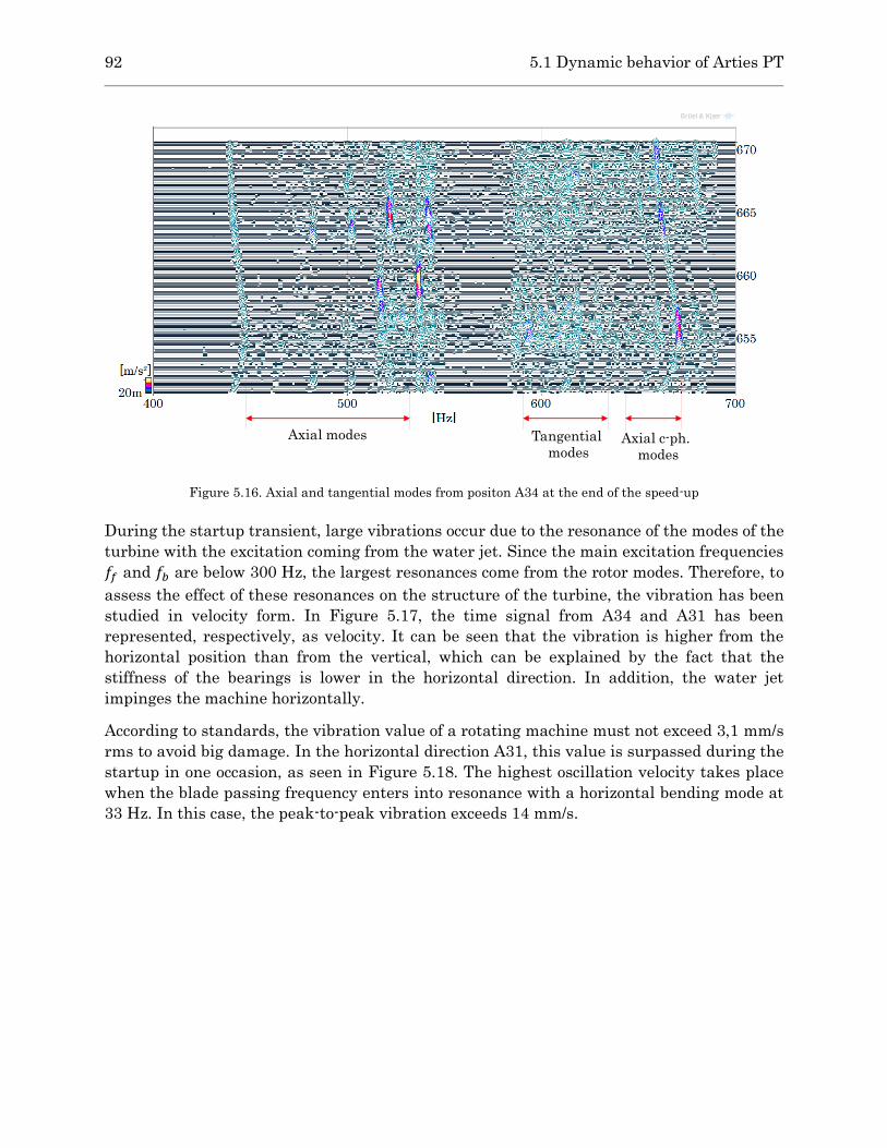
92 5.1 Dynamic behavior of Arties PT
Figure 5.16. Axial and tangential modes from positon A34 at the end of the speed-up
During the startup transient, large vibrations occur due to the resonance of the modes of the
turbine with the excitation coming from the water jet. Since the main excitation frequencies
𝑓𝑓 and 𝑓𝑏 are below 300 Hz, the largest resonances come from the rotor modes. Therefore, to
assess the effect of these resonances on the structure of the turbine, the vibration has been
studied in velocity form. In Figure 5.17, the time signal from A34 and A31 has been
represented, respectively, as velocity. It can be seen that the vibration is higher from the
horizontal position than from the vertical, which can be explained by the fact that the
stiffness of the bearings is lower in the horizontal direction. In addition, the water jet
impinges the machine horizontally.
According to standards, the vibration value of a rotating machine must not exceed 3,1 mm/s
rms to avoid big damage. In the horizontal direction A31, this value is surpassed during the
startup in one occasion, as seen in Figure 5.18. The highest oscillation velocity takes place
when the blade passing frequency enters into resonance with a horizontal bending mode at
33 Hz. In this case, the peak-to-peak vibration exceeds 14 mm/s.
Axial modes Tangential
modesAxial c-ph.
modes

Dynamic analysis of Pelton turbines 93
Figure 5.17. Velocity time signal from A31(top) and A34 (bottom)
Figure 5.18. Overall vibration values during startup from A31 (red) and A34 (blue)
580
[s] (Relative Time)
590
[s] (Relative Time)
600
[s] (Relative Time)
610
[s] (Relative Time)
620
[s] (Relative Time)
630
[s] (Relative Time)
640
[s] (Relative Time)
0
500u
1m
1.5m
2m
2.5m
3m
3.5m
4m
Cursor values
X: 641.296 s
Y: 124.386u m/s
Z: 0
4

94 5.1 Dynamic behavior of Arties PT
5.1.3. Steady operation
The dynamic behavior of the turbine under load conditions will be studied in this section. To
do so, the excitation of the runner modes will be identified and analyzed from the bearings
and compared between partial load and maximum load. After that, the frequency ranges
corresponding to the different runner modes will be determined. The overall vibration levels
of every frequency band will be obtained to see how the excitation of the runner modes
changes with the power delivered by the turbine. These will be analyzed to understand the
characteristics of the jet excitation and its repercussion on the structural integrity of the
turbine.
The waterfall of the spectra at partial load from position A34 is showed in Figure 5.19. In the
lower range of frequencies, typical excitations from the electrical grid can be seen at 100 Hz
and harmonics. The main excitation comes from the jet impingement at the bucket passing
frequency (220 Hz) and its first harmonic at 440 Hz.
Figure 5.19. Spectra waterfall from position A34 of Arties at minimum load
The frequencies between 10 and 300 Hz have been studied as velocity from position A31 at
partial and full load, as seen in Figure 5.20. Looking at the top image it can be seen that the
vibration is dominated by the constant excitation at the frequency of rotation 𝑓𝑓 (10 Hz), the
bucket passing frequency 𝑓𝑏 (220 Hz), the pole passing frequency 𝑓𝑝 (100 Hz) and the
corresponding harmonics. Moreover, the periodic excitation of the rotor bending modes can
be seen between 100 and 130 Hz. This vibration fluctuates over time, what means a different
frequency is excited at every instant, corresponding to the different variants of the same
bending mode.
When working at full load (bottom image), the vibration levels increase. The frequencies
excited are the same as the partial load operation, but the magnitudes of each one of them
vary in different ways. The unbalance force at 𝑓𝑓 doesn’t increase, since its value only depends
on the velocity and the unbalanced mass in rotation, which are the same as in partial load.

Dynamic analysis of Pelton turbines 95
However, the frequencies that are related to the force of the jet (bucket passing frequency
and turbine modes) are higher. The frequencies around 30 and 120 Hz stand out due to the
excitation of two types of rotor bending modes, which have more vibration for the increased
force of the jet. The bucket passing frequency also increases at full load operation.
Figure 5.20. Spectra waterfall from position A31. Top, partial load and bottom, full load
The vibration in the range between 10 and 400 Hz has been represented as acceleration in
Figure 5.21 as a wavelet. Wavelets provide a high resolution in the time domain and are
useful to detect the pulses of an excitation at a certain frequency, what cannot be seen with
FFT. In the figure, it is clearly seen that the main excitations at 120 and 220 Hz are not
constant over time and have a pulsating frequency. Demodulating the ranges 119-121 Hz and
219-221 Hz, pulses at 10 and 20 Hz are obtained, respectively. Since these can be related to
the rotational speed of the turbine, this means that at every turn some parts of the runner
vibrate more than others, what causes the vibration to increase.
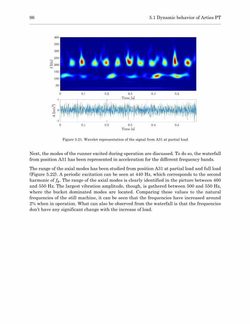
96 5.1 Dynamic behavior of Arties PT
Figure 5.21. Wavelet representation of the signal from A31 at partial load
Next, the modes of the runner excited during operation are discussed. To do so, the waterfall
from position A31 has been represented in acceleration for the different frequency bands.
The range of the axial modes has been studied from position A31 at partial load and full load
(Figure 5.22). A periodic excitation can be seen at 440 Hz, which corresponds to the second
harmonic of 𝑓𝑏. The range of the axial modes is clearly identified in the picture between 460
and 550 Hz. The largest vibration amplitude, though, is gathered between 500 and 550 Hz,
where the bucket dominated modes are located. Comparing these values to the natural
frequencies of the still machine, it can be seen that the frequencies have increased around
2% when in operation. What can also be observed from the waterfall is that the frequencies
don’t have any significant change with the increase of load.
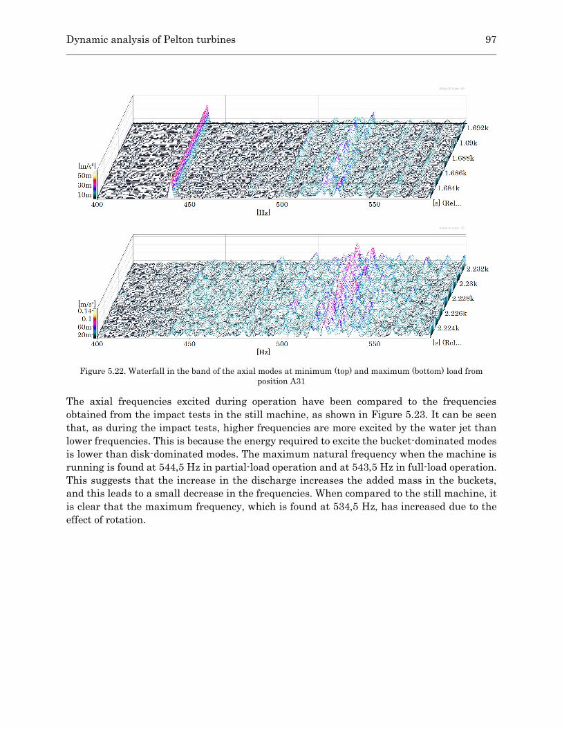
Dynamic analysis of Pelton turbines 97
Figure 5.22. Waterfall in the band of the axial modes at minimum (top) and maximum (bottom) load from
position A31
The axial frequencies excited during operation have been compared to the frequencies
obtained from the impact tests in the still machine, as shown in Figure 5.23. It can be seen
that, as during the impact tests, higher frequencies are more excited by the water jet than
lower frequencies. This is because the energy required to excite the bucket-dominated modes
is lower than disk-dominated modes. The maximum natural frequency when the machine is
running is found at 544,5 Hz in partial-load operation and at 543,5 Hz in full-load operation.
This suggests that the increase in the discharge increases the added mass in the buckets,
and this leads to a small decrease in the frequencies. When compared to the still machine, it
is clear that the maximum frequency, which is found at 534,5 Hz, has increased due to the
effect of rotation.

98 5.1 Dynamic behavior of Arties PT
400
[Hz]
450
[Hz]
500
[Hz]
550
[Hz]
0.5
1
1.5
2
2.5
3
3.5
4
4.55 Cursor values
X: 492.000 Hz
Y: 0.433 (m/s^2)/N
4
Figure 5.23. Comparison between axial frequencies in the machine still (top), during part-load operation
(middle) and full-load operation (bottom)
The tangential modes and the axial c-ph. modes have been analyzed from position A31 and
represented in Figure 4.25. These are clearly excited between 600 and 700 Hz. Even though
the main excitations are found in the harmonics of the frequency of rotation, the frequencies
excited at every instant are different. In this case, it is difficult to discern the limits between
the different types of modes. Thus, it is not possible to quantify the variation of the
frequencies due to rotation and added mass.
The range of the tangential modes has been represented as a wavelet waterfall in Figure
5.25. As seen previously, the excitation is not constant and shows many fluctuations, possibly
due to differences in the excitability of the buckets.
400
[Hz]
450
[Hz]
500
[Hz]
550
[Hz]
5m
10m
15m
20m
25m
30m
35m
40m
45mCursor values
X: 544.500 Hz
Y: 46.615m m/s²
Z: 1.703k s
4
400
[Hz]
450
[Hz]
500
[Hz]
550
[Hz]
20m
40m
60m
80m
0.1
0.12
Cursor values
X: 533.500 Hz
Y: 56.312m m/s²
Z: 2.224k s
4

Dynamic analysis of Pelton turbines 99
Figure 5.24. Excitation of tangential and axial c-ph. modes at minimum (top) and maximum (bottom) load from
position A31
Figure 5.25. Wavelet representation of the tangential modes excited from A31
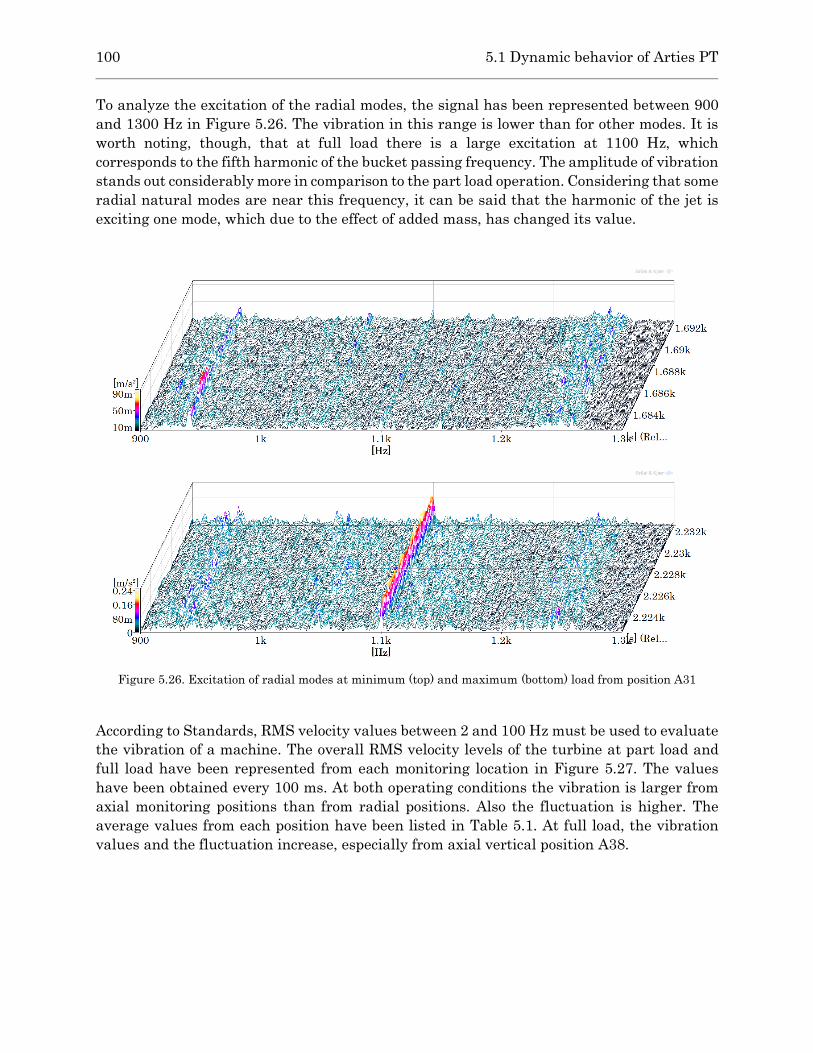
100 5.1 Dynamic behavior of Arties PT
To analyze the excitation of the radial modes, the signal has been represented between 900
and 1300 Hz in Figure 5.26. The vibration in this range is lower than for other modes. It is
worth noting, though, that at full load there is a large excitation at 1100 Hz, which
corresponds to the fifth harmonic of the bucket passing frequency. The amplitude of vibration
stands out considerably more in comparison to the part load operation. Considering that some
radial natural modes are near this frequency, it can be said that the harmonic of the jet is
exciting one mode, which due to the effect of added mass, has changed its value.
Figure 5.26. Excitation of radial modes at minimum (top) and maximum (bottom) load from position A31
According to Standards, RMS velocity values between 2 and 100 Hz must be used to evaluate
the vibration of a machine. The overall RMS velocity levels of the turbine at part load and
full load have been represented from each monitoring location in Figure 5.27. The values
have been obtained every 100 ms. At both operating conditions the vibration is larger from
axial monitoring positions than from radial positions. Also the fluctuation is higher. The
average values from each position have been listed in Table 5.1. At full load, the vibration
values and the fluctuation increase, especially from axial vertical position A38.

Dynamic analysis of Pelton turbines 101
Table 5.1. Overall RMS velocity values of Arties from different monitoring positions
Location RMS Partial
load [mm/s]
RMS Full
load [mm/s]
Ratio
A31 0,170 0,430 2,53
A34 0,112 0,402 3,6
A35 0,235 0,710 3,02
A38 0,430 1,020 2,37
Figure 5.27. Overall RMS velocity values from positions A31 (red), A34 (blue), A35 (green) and A38 (orange) at
partial load (left) and full load (right)
Two frequency bands have been selected to see the energy used to excite each type of turbine
mode, according to the information obtained from the spectra. The RMS velocity values have
been obtained. They have been represented for the band of the axial modes [480-540 Hz] in
Figure 5.28 and for the band of the tangential modes [600-670 Hz] in Figure 5.29. Operation
at partial load and at maximum load can be compared. The RMS average values are listed in
Table 5.2 and Table 5.3, respectively. It is interesting to see that, even if the global RMS
values are low comparatively to other positions, A34 has the best sensitivity to both axial
modes and tangential modes.
Table 5.2. Averaged RMS values for the axial modes from every position at partial and full load
Location RMS Partial
load [mm/s]
Ratio to
total energy
RMS Full
load [mm/s]
Ratio to
total energy
A31 0,014 8,2% 0,060 14%
A34 0,032 28,6% 0,084 21%
A35 0,008 3,4% 0,028 4%
A38 0,017 4% 0,070 6,9%
1.685k
[s] (Relative Time)
1.69k
[s] (Relative Time)
1.695k
[s] (Relative Time)
1.7k
[s] (Relative Time)
0
50u
100u
150u
200u
250u
300u
350u
400u
450u
[m/s]
2.224k
[s] (Relative Time)
2.228k
[s] (Relative Time)
2.232k
[s] (Relative Time)
2.236k
[s] (Relative Time)
2.24k
[s] (Relative Time)
0
200u
400u
600u
800u
1m
1.2m
[m/s]

102 5.1 Dynamic behavior of Arties PT
Figure 5.28. Overall RMS velocity values in the band of axial modes from positions A31 (red), A34 (blue), A35
(green) and A38 (orange) at partial load (left) and full load (right)
Table 5.3. Averaged RMS values for the tangential modes from every position at partial and full load
Location RMS Partial
load [mm/s]
Ratio to
total energy
RMS Full
load [mm/s]
Ratio to
total energy
A31 0,028 16,5% 0,108 25%
A34 0,028 25% 0,128 31,8%
A35 0,028 11,9% 0,092 13%
A38 0,016 3,7% 0,062 6%
Figure 5.29. Overall RMS velocity values in the band of tangential modes from positions A31 (red), A34 (blue),
A35 (green) and A38 (orange) at partial load (left) and full load (right)
1.685k
[s] (Relative Time)
1.69k
[s] (Relative Time)
1.695k
[s] (Relative Time)
1.7k
[s] (Relative Time)
0
5u
10u
15u
20u
25u
30u
35u
40u
45u
[m/s]
2.224k
[s] (Relative Time)
2.228k
[s] (Relative Time)
2.232k
[s] (Relative Time)
2.236k
[s] (Relative Time)
2.24k
[s] (Relative Time)
0
20u
40u
60u
80u
100u
[m/s]
1.685k
[s] (Relative Time)
1.69k
[s] (Relative Time)
1.695k
[s] (Relative Time)
1.7k
[s] (Relative Time)
0
4u
8u
12u
16u
20u
24u
28u
32u
[m/s]
2.224k
[s] (Relative Time)
2.228k
[s] (Relative Time)
2.232k
[s] (Relative Time)
2.236k
[s] (Relative Time)
2.24k
[s] (Relative Time)
0
20u
40u
60u
80u
100u
120u
140u
[m/s]

Dynamic analysis of Pelton turbines 103
5.2. Dynamic behavior of Moncabril PT
In this section the operation of the Pelton turbine of Moncabril has been studied. The setup
of this machine is different from Arties because there is only one runner and this is operated
by two nozzles. Moreover, the directions of the jets are different. The vibrations of the
machine were recorded during the startup and at different operating loads, from minimum
to maximum. In this case, two transients take place, one from the entrance of the first jet
and one for the second jet. Both transients will be studied to see the effect they have on the
vibration of the buckets. After that, the vibration at minimum and maximum load will be
analyzed to check the effects of the load on the runner modes and the vibration.
5.2.1. On-site measurements
The instrumentation used in the Pelton turbine of Moncabril was the same used in the impact
tests, described in Chapter 3. To carry out the tests in operation, four accelerometers were
placed on the turbine bearing in two radial positions and two axial positions: A13, A14, A16
and A17. The vibration recorded by accelerometer A14 during the whole test is showed in
Figure 5.30. The turbine was set in motion by opening one of the nozzles (1). After achieving
the nominal speed of 600 min-1, the machine was operated at Speed No load during
approximately 5 minutes. During this time, the generator was excited magnetically (2). At
(3), the machine was connected to the electrical grid and operated at the minimum load of 1
MW. After a period of time, the load was increased to 3 MW, and then to 4,8 MW. Before
increasing the load to 6 MW, the second nozzle was opened. This can be seen in the time
signal by the increase of the vibration levels (4). After that, the load was increased to 9 MW,
and, finally, to maximum load, 12 MW.
Figure 5.30. Time signal of the whole test from position A14

104 5.2 Dynamic behavior of Moncabril PT
5.2.2. Startup transient
The acceleration time signal of the startup transient measured from position A14 is showed
in Figure 5.31. At the start of the excitation, the first impact of the water particles can be
identified. The levels increase when the machine starts rotating due to the resonance with
different turbine modes, and then decreases as it approaches its nominal speed. The spectra
waterfall from the same position is in Figure 5.32. The range of the rotor modes (lower
frequencies) and the runner modes (higher frequencies) can be discerned.
Figure 5.31. Time signal during the startup transient from A14
Figure 5.32. Waterfall of the startup transient from position A14

Dynamic analysis of Pelton turbines 105
First, the initial impact of the water particles will be studied in the range of the runner
modes. This is the first and purest excitation of the runner modes during operation, and from
this, the modes of the buckets can be identified.
In Moncabril Pelton turbine, the most excited frequencies are found in the range of the
tangential modes, as seen in Figure 5.32. The axial modes, unlike the case of the machine in
Arties, don’t show a large excitation after the first impact. Taking a closer look at the first
seconds between 680 and 770 Hz, several peaks can be identified (Figure 5.33), which
correspond to the tangential modes in phase and in counter-phase of the runner. The values
of the frequencies are very similar to the still machine, and the highest peaks are detected
from the radial vertical position A14, which was proved to be the best monitoring location
during the impact tests. It can also be seen that the tangential in phase modes are more
excited than the torsional modes.
Figure 5.33. Tangential modes excited after the first impact
Compared to the Pelton turbine in Arties, the axial counter-phase modes in Moncabril appear
at much higher frequencies than the tangential modes, and thus the limits can be more easily
discerned. In Figure 5.34, the range between 860 and 940 Hz is showed. It is proved that the
axial counter-phase modes are excited in the first impact, and that the frequencies are the
same as the still machine. Two main frequencies are excited at 903 and 910 Hz, which
correspond to the frequencies of the buckets impinged by the jet. The radial vertical position
A14 has the highest sensitivity to that vibration.
Tangential in-phase Tangential c-ph.

106 5.2 Dynamic behavior of Moncabril PT
Figure 5.34. Axial counter-phase modes after initial impact
During the first seconds of the machine speed-up, the load applied on the buckets excites
many modes. Since the rotational speed is much lower than the nominal speed, the jet enters
the buckets with a relative velocity that is still too fast, and the load applied is high. During
this time, the vibration is also mixed between the different buckets.
The lower range of frequencies during startup has been analyzed from position A13 (Figure
5.35). The increasing bucket passing frequency can be clearly seen. Rotor modes are excited
by the 𝑓𝑏 at 40 Hz, 70 Hz, 120 Hz and 155 Hz.
Figure 5.35. Startup from position A13
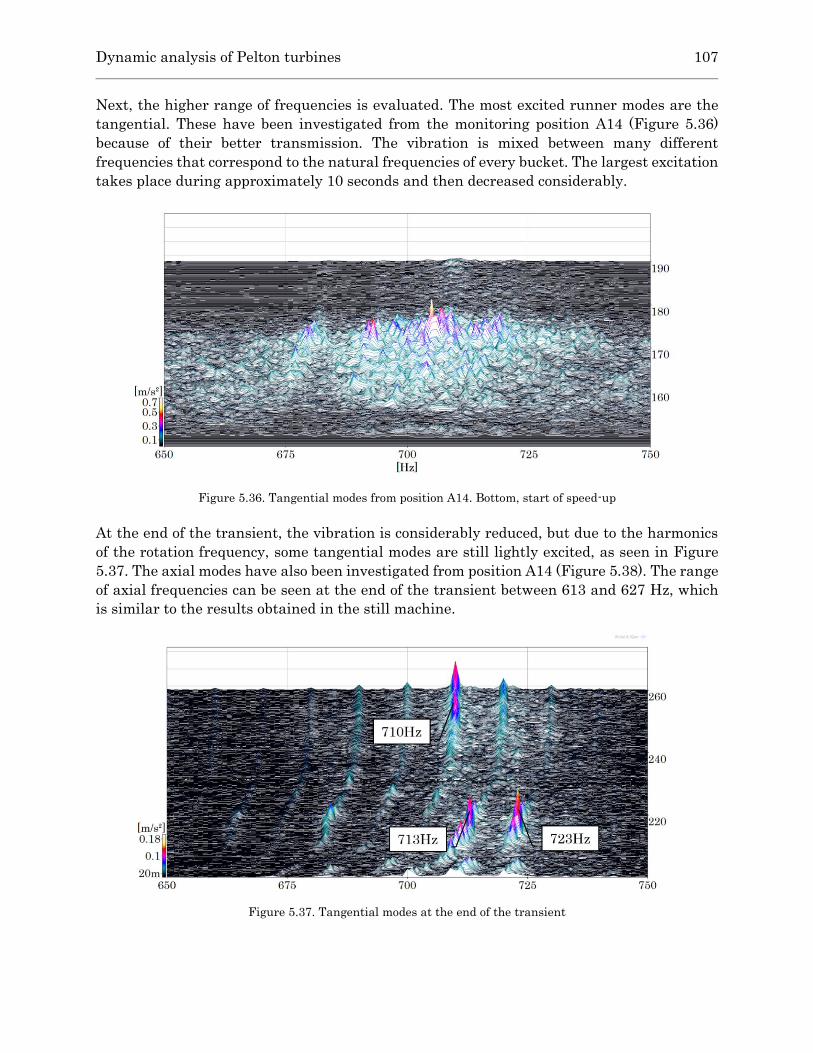
Dynamic analysis of Pelton turbines 107
Next, the higher range of frequencies is evaluated. The most excited runner modes are the
tangential. These have been investigated from the monitoring position A14 (Figure 5.36)
because of their better transmission. The vibration is mixed between many different
frequencies that correspond to the natural frequencies of every bucket. The largest excitation
takes place during approximately 10 seconds and then decreased considerably.
Figure 5.36. Tangential modes from position A14. Bottom, start of speed-up
At the end of the transient, the vibration is considerably reduced, but due to the harmonics
of the rotation frequency, some tangential modes are still lightly excited, as seen in Figure
5.37. The axial modes have also been investigated from position A14 (Figure 5.38). The range
of axial frequencies can be seen at the end of the transient between 613 and 627 Hz, which
is similar to the results obtained in the still machine.
Figure 5.37. Tangential modes at the end of the transient

108 5.2 Dynamic behavior of Moncabril PT
Figure 5.38. Axial modes at the end of the transient
The effect of the transient on the structure can be evaluated from the velocity values of the
vibration (see Figure 5.39). The horizontal radial position A13 shows the largest vibration
levels. The maximum peak-to-peak velocities reach the value of 14 mm/s. In these instants,
rotor bending modes are excited by the bucket passing frequency. To assess the peril of this
situation on the structure, the stress distribution must be studied by numerical models and
the most affected zones must be determined.
Figure 5.39. Overall velocity vibration levels from A13
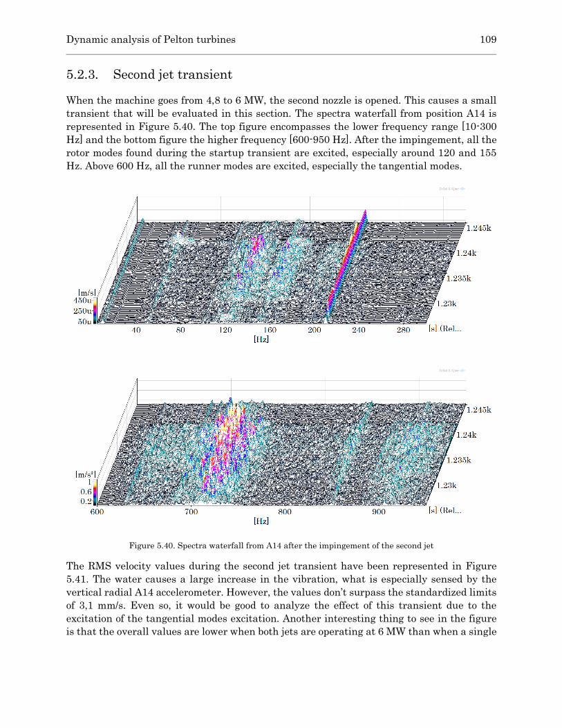
Dynamic analysis of Pelton turbines 109
5.2.3. Second jet transient
When the machine goes from 4,8 to 6 MW, the second nozzle is opened. This causes a small
transient that will be evaluated in this section. The spectra waterfall from position A14 is
represented in Figure 5.40. The top figure encompasses the lower frequency range [10-300
Hz] and the bottom figure the higher frequency [600-950 Hz]. After the impingement, all the
rotor modes found during the startup transient are excited, especially around 120 and 155
Hz. Above 600 Hz, all the runner modes are excited, especially the tangential modes.
Figure 5.40. Spectra waterfall from A14 after the impingement of the second jet
The RMS velocity values during the second jet transient have been represented in Figure
5.41. The water causes a large increase in the vibration, what is especially sensed by the
vertical radial A14 accelerometer. However, the values don’t surpass the standardized limits
of 3,1 mm/s. Even so, it would be good to analyze the effect of this transient due to the
excitation of the tangential modes excitation. Another interesting thing to see in the figure
is that the overall values are lower when both jets are operating at 6 MW than when a single

110 5.2 Dynamic behavior of Moncabril PT
jet is operating at 4,5 MW. The machine is thus more balanced with both jets operating and
this causes less vibration, even if the load is larger.
Figure 5.41. Overall RMS velocity values during second jet transient
5.2.4. Steady operation
The dynamic behavior of a Pelton turbine is ruled by the modal behavior of the structure and
by the excitation coming from the various forces that are applied to them. These are difficult
to predict, especially the ones coming from the jet. In this section, the steady operation of the
Moncabril turbine has been studied. The vibration while operating at minimum load (1 MW)
and maximum load (12 MW) has been analyzed.
First, the lower frequency range has been evaluated. In Figure 5.42, the spectra waterfall
between 10 and 300 Hz is represented for both operating conditions. The main excitations
are to be seen at the rotating frequency (𝑓𝑓=10 Hz) and at the bucket passing frequency
(𝑓𝑏=210 Hz). The corresponding harmonics can also be seen. At minimum load, the excitation
of the rotor modes is not large compared to the force of the jet. However, when operating at
maximum load, the rotor modes are comparatively more excited and the vibration fluctuates
more than the minimum load operation.
1.2k
[s] (Relative Time)
1.22k
[s] (Relative Time)
1.24k
[s] (Relative Time)
1.26k
[s] (Relative Time)
1.28k
[s] (Relative Time)
200u
400u
600u
800u
1m
[m/s]
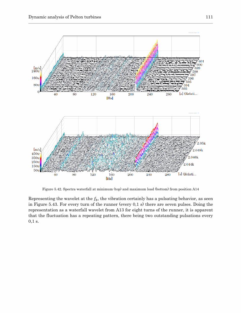
Dynamic analysis of Pelton turbines 111
Figure 5.42. Spectra waterfall at minimum (top) and maximum load (bottom) from position A14
Representing the wavelet at the 𝑓𝑏, the vibration certainly has a pulsating behavior, as seen
in Figure 5.43. For every turn of the runner (every 0,1 s) there are seven pulses. Doing the
representation as a waterfall wavelet from A13 for eight turns of the runner, it is apparent
that the fluctuation has a repeating pattern, there being two outstanding pulsations every
0,1 s.

112 5.2 Dynamic behavior of Moncabril PT
Figure 5.43. Wavelet of the vibration from A14 at the lower frequency range
Figure 5.44. Wavelet waterfall of the vibration from A13 at the lower frequency range
Next, the higher frequency range has been represented to evaluate the runner modes. The
spectra waterfalls in the ranges of the axial, tangential and axial in-phase modes are
illustrated in Figure 5.45, Figure 5.46 and Figure 5.48, respectively. In the range between
400 and 660 Hz, the second harmonic of the bucket passing frequency at 420 Hz and the axial
modes are seen. However, the excitation is low and cannot be considered important.
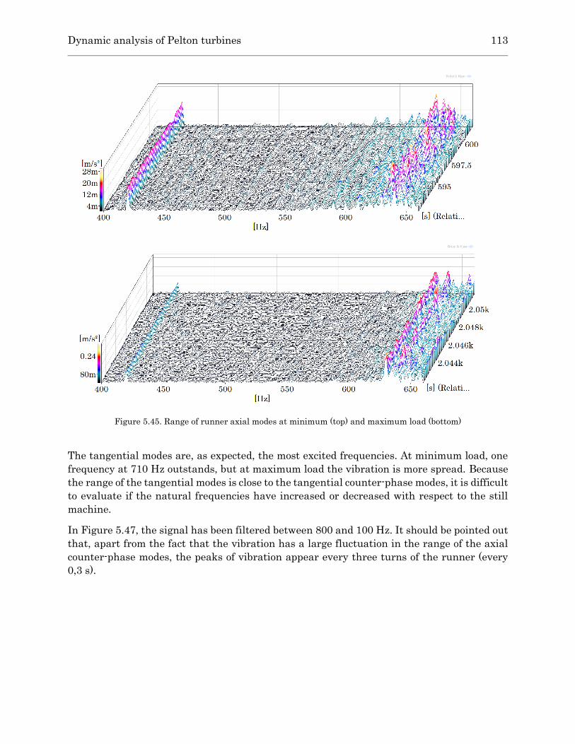
Dynamic analysis of Pelton turbines 113
Figure 5.45. Range of runner axial modes at minimum (top) and maximum load (bottom)
The tangential modes are, as expected, the most excited frequencies. At minimum load, one
frequency at 710 Hz outstands, but at maximum load the vibration is more spread. Because
the range of the tangential modes is close to the tangential counter-phase modes, it is difficult
to evaluate if the natural frequencies have increased or decreased with respect to the still
machine.
In Figure 5.47, the signal has been filtered between 800 and 100 Hz. It should be pointed out
that, apart from the fact that the vibration has a large fluctuation in the range of the axial
counter-phase modes, the peaks of vibration appear every three turns of the runner (every
0,3 s).
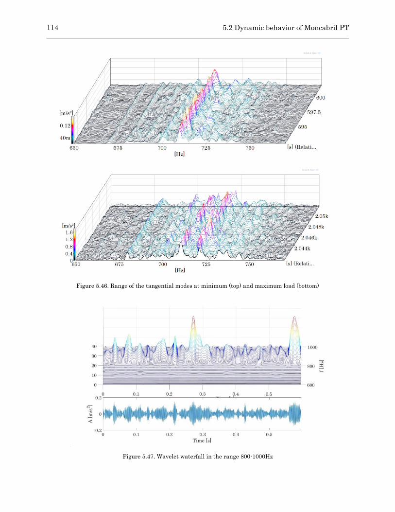
114 5.2 Dynamic behavior of Moncabril PT
Figure 5.46. Range of the tangential modes at minimum (top) and maximum load (bottom)
Figure 5.47. Wavelet waterfall in the range 800-1000Hz
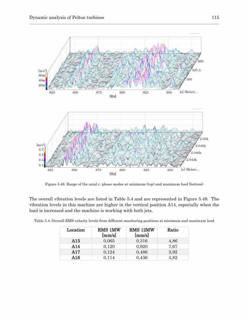
Dynamic analysis of Pelton turbines 115
Figure 5.48. Range of the axial c.-phase modes at minimum (top) and maximum load (bottom)
The overall vibration levels are listed in Table 5.4 and are represented in Figure 5.49. The
vibration levels in this machine are higher in the vertical position A14, especially when the
load is increased and the machine is working with both jets.
Table 5.4. Overall RMS velocity levels from different monitoring positions at minimum and maximum load
Location RMS 1MW
[mm/s]
RMS 12MW
[mm/s]
Ratio
A13 0,065 0,316 4,86
A14 0,120 0,920 7,67
A17 0,124 0,486 3,92
A16 0,114 0,436 3,82
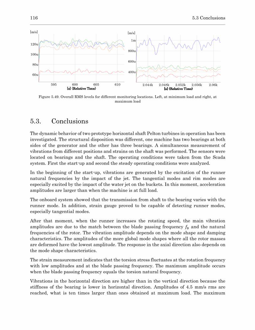
116 5.3 Conclusions
Figure 5.49. Overall RMS levels for different monitoring locations. Left, at minimum load and right, at
maximum load
5.3. Conclusions
The dynamic behavior of two prototype horizontal shaft Pelton turbines in operation has been
investigated. The structural disposition was different, one machine has two bearings at both
sides of the generator and the other has three bearings. A simultaneous measurement of
vibrations from different positions and strains on the shaft was performed. The sensors were
located on bearings and the shaft. The operating conditions were taken from the Scada
system. First the start-up and second the steady operating conditions were analyzed.
In the beginning of the start-up, vibrations are generated by the excitation of the runner
natural frequencies by the impact of the jet. The tangential modes and rim modes are
especially excited by the impact of the water jet on the buckets. In this moment, acceleration
amplitudes are larger than when the machine is at full load.
The onboard system showed that the transmission from shaft to the bearing varies with the
runner mode. In addition, strain gauge proved to be capable of detecting runner modes,
especially tangential modes.
After that moment, when the runner increases the rotating speed, the main vibration
amplitudes are due to the match between the blade passing frequency 𝑓𝑏 and the natural
frequencies of the rotor. The vibration amplitude depends on the mode shape and damping
characteristics. The amplitudes of the more global mode shapes where all the rotor masses
are deformed have the lowest amplitude. The response in the axial direction also depends on
the mode shape characteristics.
The strain measurement indicates that the torsion stress fluctuates at the rotation frequency
with low amplitudes and at the blade passing frequency. The maximum amplitude occurs
when the blade passing frequency equals the torsion natural frequency.
Vibrations in the horizontal direction are higher than in the vertical direction because the
stiffness of the bearing is lower in horizontal direction. Amplitudes of 4.5 mm/s rms are
reached, what is ten times larger than ones obtained at maximum load. The maximum
595
[s] (Relative Time)
600
[s] (Relative Time)
605
[s] (Relative Time)
610
[s] (Relative Time)
60u
80u
100u
120u
[m/s]
2.044k
[s] (Relative Time)
2.048k
[s] (Relative Time)
2.052k
[s] (Relative Time)
2.056k
[s] (Relative Time)
2.06k
[s] (Relative Time)
400u
600u
800u
1m
[m/s]

Dynamic analysis of Pelton turbines 117
response is with the mode with axial motion of the runner producing large stresses in the
coupling zone between shaft and runner.
It is proved that with the machine in operation, the runner natural frequencies can be
detected in the monitoring positions. The best positions for the best detection of them have
been assessed.
Another important topic is the variation of the runner frequencies when the turbine is in
operation due to added mass and stiffness due to centrifugal forces. In the cases studied, the
changes observed are not significant and are in the range of the scattering of natural
frequencies due to lack of precision during the runner machining.
Finally, the evolution of the band level related to each mode shape have been calculated.
In the next chapter all the knowledge obtained will be used for an upgrading of the
monitoring systems.

118 5.3 Conclusions

Chapter 6 Monitoring of Pelton turbines
Due to the massive entrance of new renewable energies (NRE), the electricity market has
changed completely. Today, hydropower plants are of paramount importance due to their
capability to absorb and supply a variable quantity of energy, depending on the electrical grid
needs. By 2030 the market share of NRE is forecast to be higher than 30% in Europe. To cope
with this increase, more flexibility is demanded to hydropower plants so that they can
respond faster to any change in demand and supply. Because the price of energy depends
much on the rapidity of hydropower plants to provide or take energy from the grid, operators
can obtain more revenues by increasing the flexibility of the turbines. However, this is
translated into the turbines operating longer in off-design conditions and increasing the
start/stop sequences. This usually means stronger excitation forces on the structure and a
faster deterioration, what may reduce the maintenance intervals and increase the costs.
In this new competitive market, managers demand more control on their assets and require
more tools to weigh the economic benefits of flexibility with the increased cost of
maintenance. Remaining useful life (RUL) estimations that are based on present and future
operational conditions (input commands, environment and loads) have to be introduced in
the current monitoring systems. It is about operation decision making according to the cost
of maintenance and price of energy. To achieve this goal, an upgrading of the actual condition
monitoring systems has to be done, so that the consequences of machine of flexibility can be
estimated.
In this chapter, the extensive structural and dynamic analysis of Pelton turbines carried out
in the other chapters will be used for an optimization of the existing condition monitoring
systems.
An advanced condition monitoring system has to be able to identify situations of abnormal
turbine operation that may lead to failure and to detect incipient damage in real time. As
indicated in the beginning, the runner is the component more prone to have damage.
Therefore, the feasibility to detect, evaluate and follow up the runner vibrations constitutes
the main challenge.
120 6.1 General approach to CM of hydro turbines
The strategy to implement an advanced condition monitoring system is discussed in this
chapter. First step is to analyze typical vibration signatures of Pelton turbines and to
determine how they change with the most common types of damage. Knowing the dynamic
behavior of the machine, two methods are possible; one is through the analysis of field data
(if available) and the other generating synthetic damage in calibrated models. Field data
analysis of vibration signatures before and after maintenance results very useful to extract
symptoms of damage in vibration signatures. The historic of several machines have been
studied for that. Second step is to select the condition indicators. In this thesis, the choice of
spectral bands associated to the runner vibration will be discussed with some examples.
6.1. General approach to CM of hydro turbines
The goal for a condition monitoring system is:
- Identification of operating condition with abnormal situations that can lead to damage.
- Detection and diagnosis of (incipient) damage.
- Prognosis. The ultimate objective is to calculate the residual useful time (RUL) depending
on the operating conditions so that the cost of operation can be estimated.
An advanced condition monitoring system has to be able to detect in real-time incipient
damage and abnormal operation that can lead to failure and estimate the RUL according to
the possible future operating conditions. With this information the operating conditions
and/or maintenance tasks can be decided. All this process has to be done in “real time”,
simulating different scenarios of operation each one with a degradation model.
In Figure 6.1 a general sketch of an ideal monitoring system has been represented.
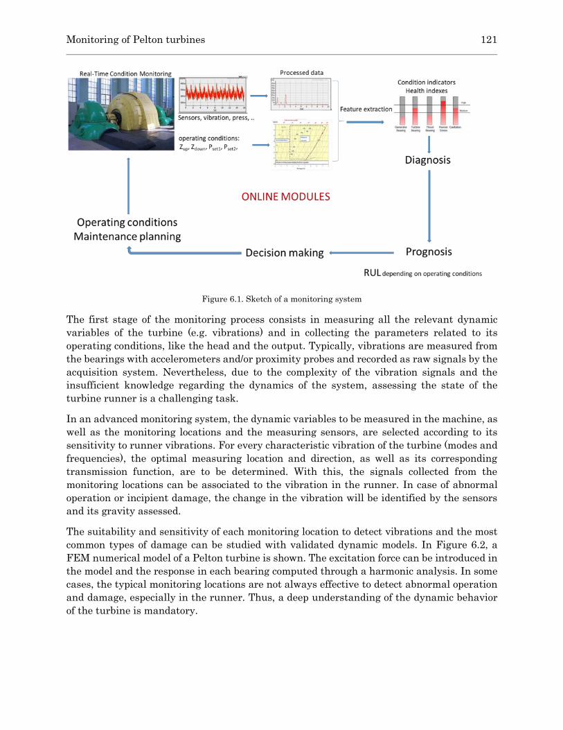
Monitoring of Pelton turbines 121
Figure 6.1. Sketch of a monitoring system
The first stage of the monitoring process consists in measuring all the relevant dynamic
variables of the turbine (e.g. vibrations) and in collecting the parameters related to its
operating conditions, like the head and the output. Typically, vibrations are measured from
the bearings with accelerometers and/or proximity probes and recorded as raw signals by the
acquisition system. Nevertheless, due to the complexity of the vibration signals and the
insufficient knowledge regarding the dynamics of the system, assessing the state of the
turbine runner is a challenging task.
In an advanced monitoring system, the dynamic variables to be measured in the machine, as
well as the monitoring locations and the measuring sensors, are selected according to its
sensitivity to runner vibrations. For every characteristic vibration of the turbine (modes and
frequencies), the optimal measuring location and direction, as well as its corresponding
transmission function, are to be determined. With this, the signals collected from the
monitoring locations can be associated to the vibration in the runner. In case of abnormal
operation or incipient damage, the change in the vibration will be identified by the sensors
and its gravity assessed.
The suitability and sensitivity of each monitoring location to detect vibrations and the most
common types of damage can be studied with validated dynamic models. In Figure 6.2, a
FEM numerical model of a Pelton turbine is shown. The excitation force can be introduced in
the model and the response in each bearing computed through a harmonic analysis. In some
cases, the typical monitoring locations are not always effective to detect abnormal operation
and damage, especially in the runner. Thus, a deep understanding of the dynamic behavior
of the turbine is mandatory.

122 6.1 General approach to CM of hydro turbines
Figure 6.2. Dynamic model to determine the response in the monitoring positions to the excitation generated
during the operation of the machine
The acquired raw signals are processed to extract basic features that indicate fault growth
or damage. Typical signal processing uses time-domain and frequency-domain techniques
like Fast Fourier Transforms (FFT) algorithms and other signal processing methods, like
time-frequency transforms or Frequency Response Functions (FRF). Overall RMS
amplitudes, spectral bands, statistical factors and time-domain parameters are extracted.
With the vibration features, condition indicators can be calculated, which can be effective to
detect incipient damage. These indicators are trended and compared to some alarm and trip
levels (Figure 6.3). After overpassing the alarm threshold, the diagnostics have to be done.
Figure 6.3. Trend analysis of a spectral band detecting damage, the diagnostic and the repair
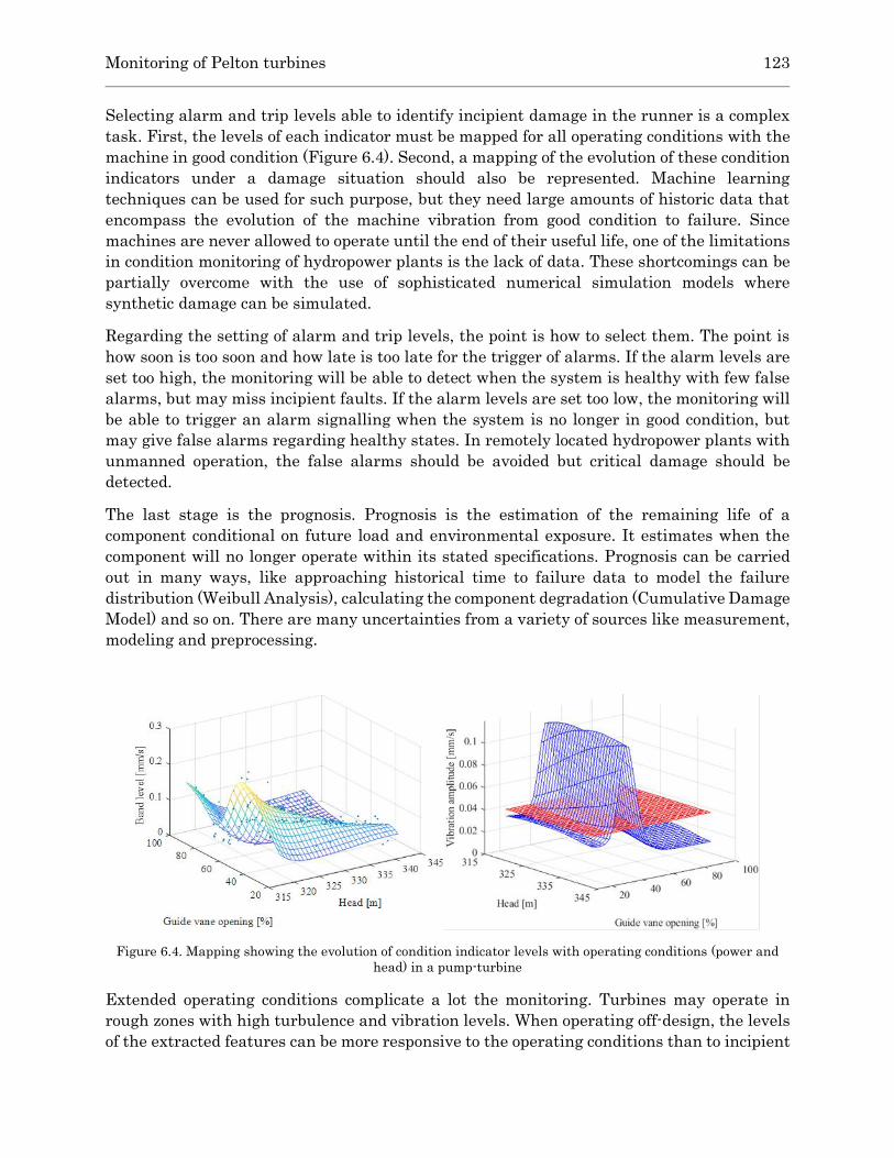
Monitoring of Pelton turbines 123
Selecting alarm and trip levels able to identify incipient damage in the runner is a complex
task. First, the levels of each indicator must be mapped for all operating conditions with the
machine in good condition (Figure 6.4). Second, a mapping of the evolution of these condition
indicators under a damage situation should also be represented. Machine learning
techniques can be used for such purpose, but they need large amounts of historic data that
encompass the evolution of the machine vibration from good condition to failure. Since
machines are never allowed to operate until the end of their useful life, one of the limitations
in condition monitoring of hydropower plants is the lack of data. These shortcomings can be
partially overcome with the use of sophisticated numerical simulation models where
synthetic damage can be simulated.
Regarding the setting of alarm and trip levels, the point is how to select them. The point is
how soon is too soon and how late is too late for the trigger of alarms. If the alarm levels are
set too high, the monitoring will be able to detect when the system is healthy with few false
alarms, but may miss incipient faults. If the alarm levels are set too low, the monitoring will
be able to trigger an alarm signalling when the system is no longer in good condition, but
may give false alarms regarding healthy states. In remotely located hydropower plants with
unmanned operation, the false alarms should be avoided but critical damage should be
detected.
The last stage is the prognosis. Prognosis is the estimation of the remaining life of a
component conditional on future load and environmental exposure. It estimates when the
component will no longer operate within its stated specifications. Prognosis can be carried
out in many ways, like approaching historical time to failure data to model the failure
distribution (Weibull Analysis), calculating the component degradation (Cumulative Damage
Model) and so on. There are many uncertainties from a variety of sources like measurement,
modeling and preprocessing.
Figure 6.4. Mapping showing the evolution of condition indicator levels with operating conditions (power and
head) in a pump-turbine
Extended operating conditions complicate a lot the monitoring. Turbines may operate in
rough zones with high turbulence and vibration levels. When operating off-design, the levels
of the extracted features can be more responsive to the operating conditions than to incipient

124 6.2 Condition monitoring of Pelton turbines
damage. These abnormal operating conditions have to be identified and the effects on the
machine components estimated.
Fortunately, Pelton turbines have a broad operating range (between 20 and 100%) with good
efficiency. Unless they are working at very low load when the jet may be asymmetric or at
very high load where the force is very large, the behavior is quite good. In the next section
the monitoring of Pelton turbines is analyzed.
6.2. Condition monitoring of Pelton turbines
First step is to analyze typical vibration signatures of Pelton turbines and to determine how
these signatures change with the most common types of damage. The vibration generated
depends on the excitation forces and on the structural response (Figure 6.5).
Figure 6.5. Vibration generation sketch
In Figure 6.6, a typical spectral signature of a Pelton turbine rotating at 600 min-1, with 22
buckets has been represented. Different types of excitation forces are generated during the
operation of the turbine, which can be classified depending on their origin as mechanical,
hydraulic or electromagnetic. Mechanical excitations are produced by unbalance and
misalignment and are found at the frequency of rotation 𝑓𝑓. This is defined as
𝑓𝑓 =
𝑁
60= 10Hz Eq. 6.1
Where 𝑁 is the rotating speed in min-1. Vibrations of hydraulic origin are also identified in
the spectrum. Unlike reaction turbines, Pelton turbines are not subjected to pressure
changes, as they are set up in an open casing. Instead, the main forces affecting the structure
are the ones coming from the water jet impacts on the runner. The frequency at which the jet
impinges the structure depends on the rotating speed of the wheel and on the number of
buckets. It can be defined by the following equation
𝑓𝑏 = 𝑛 · 𝑧𝑏 · 𝑓𝑓 = 220𝑛Hz Eq. 6.2
where 𝑓𝑏 is the frequency of the vibration generated on the wheel by the impact of the jet
(bucket passing frequency), 𝑧𝑏 is the number of the wheel buckets and 𝑓 is the shaft rotating
frequency. 𝑛 stands for the harmonics of the exciting force (𝑛 =1,2,3…). Other vibrations

Monitoring of Pelton turbines 125
identified are the ones related to the structural response, like rotor eigenfrequencies. At
higher frequencies, some broadband vibrations can also be seen.
Figure 6.6. Typical spectral vibration signature in a Pelton turbine
From these signals some features can be extracted and used for monitoring purposes, like
spectral bands amplitudes and peak to peak values. Overall vibration levels are not sensitive
enough to detect incipient damage. Potentially serious problems can develop within the
turbine and have a negligible effect on the level of the overall vibration. Anyway, they are a
reference to be considered when setting vibration monitoring. In Figure 6.7, the vibration
limits recommended by ISO Standards are indicated.
Figure 6.7. ISO 10816-5. Group 1 horizontal machines with vibration limits
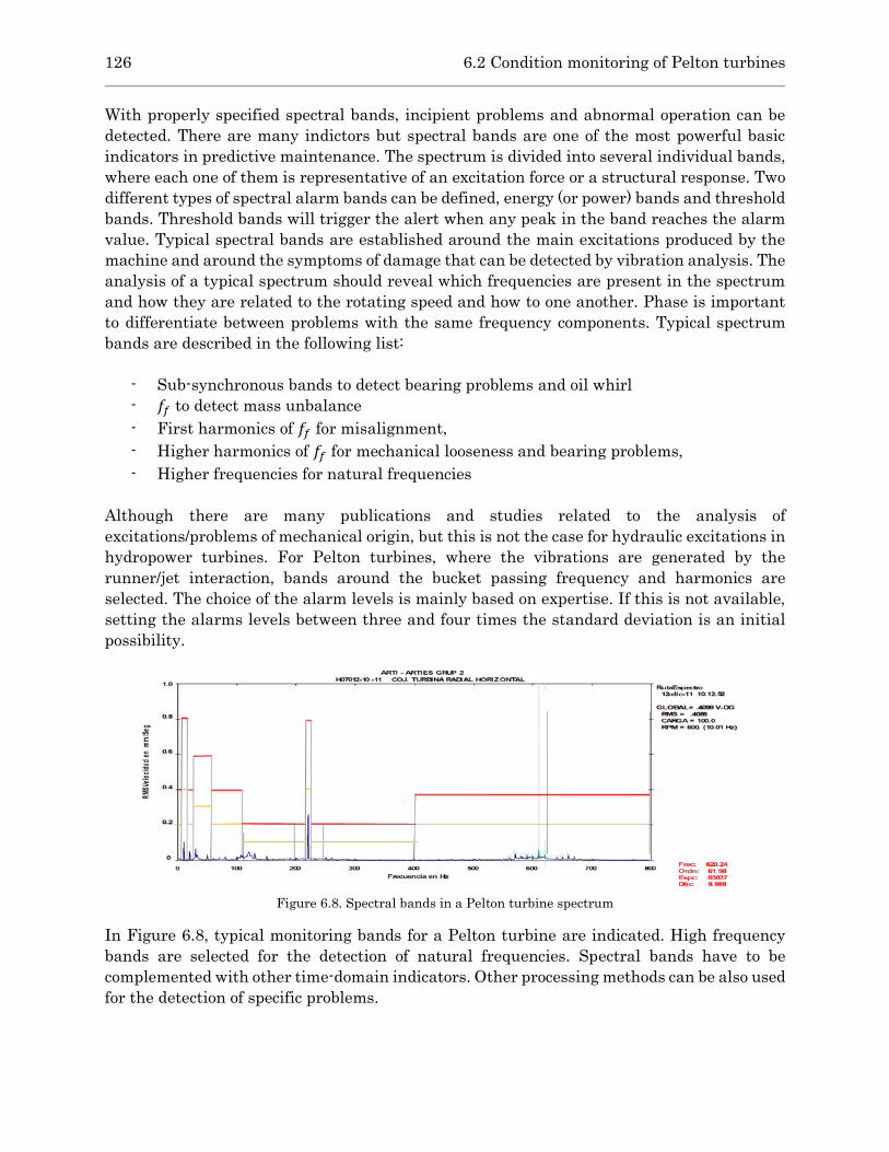
126 6.2 Condition monitoring of Pelton turbines
With properly specified spectral bands, incipient problems and abnormal operation can be
detected. There are many indictors but spectral bands are one of the most powerful basic
indicators in predictive maintenance. The spectrum is divided into several individual bands,
where each one of them is representative of an excitation force or a structural response. Two
different types of spectral alarm bands can be defined, energy (or power) bands and threshold
bands. Threshold bands will trigger the alert when any peak in the band reaches the alarm
value. Typical spectral bands are established around the main excitations produced by the
machine and around the symptoms of damage that can be detected by vibration analysis. The
analysis of a typical spectrum should reveal which frequencies are present in the spectrum
and how they are related to the rotating speed and how to one another. Phase is important
to differentiate between problems with the same frequency components. Typical spectrum
bands are described in the following list:
- Sub-synchronous bands to detect bearing problems and oil whirl
- 𝑓𝑓 to detect mass unbalance
- First harmonics of 𝑓𝑓 for misalignment,
- Higher harmonics of 𝑓𝑓 for mechanical looseness and bearing problems,
- Higher frequencies for natural frequencies
Although there are many publications and studies related to the analysis of
excitations/problems of mechanical origin, but this is not the case for hydraulic excitations in
hydropower turbines. For Pelton turbines, where the vibrations are generated by the
runner/jet interaction, bands around the bucket passing frequency and harmonics are
selected. The choice of the alarm levels is mainly based on expertise. If this is not available,
setting the alarms levels between three and four times the standard deviation is an initial
possibility.
Figure 6.8. Spectral bands in a Pelton turbine spectrum
In Figure 6.8, typical monitoring bands for a Pelton turbine are indicated. High frequency
bands are selected for the detection of natural frequencies. Spectral bands have to be
complemented with other time-domain indicators. Other processing methods can be also used
for the detection of specific problems.

Monitoring of Pelton turbines 127
For diagnosis and prognosis, the change of the aforementioned indicators with the most
common types of damage is necessary. This information should be obtained from the
monitoring of actual machines. For that purpose, a systematic analysis before and after
repair comparing the changes and knowing the damage found during the outage is very
informative. Usually this information is difficult to obtain and is not complete enough to
describe all types of damage. Apart from that, power plants are not allowed to operate beyond
their maintenance limit, what makes it difficult to know how the monitoring parameters
change when the turbine is in an advanced degradation state.
As indicated above, another possibility to complement the field data is to have a numerical
model that simulates the dynamic behavior of the whole machine. The structural response
(deformations, vibrations, strains) to the variable dynamic forces acting on the machine
during operation can be calculated. Physics-based numerical model can be used to simulate
types of damage not found in the machine (synthetic damage generation). This analysis
enables determining how all the components of the machine are deforming when the turbine
is in operation, and, at the end, allows seeing which locations of the wheel are more prone to
suffer fatigue problems. However, developing models is not trivial and refined models may
be computationally expensive to run. CFD computation of the jet and its application to the
FEM model is not an easy task and impractical for real-time applications. Moreover, models
have to be tuned with field data.
A critical issue when monitoring a Pelton turbine is the detection of runner problems. The
runner is receiving directly the high speed jet of water and is the turbine component more
prone to have damage. In the previous chapters, the feasibility to detect runner vibrations
from the monitoring positions has been proved. Moreover, the best sensor type and location
has been checked. This information will be used to upgrade the monitoring system.
Once proved that the runner can be monitored from the bearings, the next step consists in
knowing which are the most common types of damage. For that purpose, the monitoring
information and data obtained after more than twenty years of monitoring have been
analyzed. The main types of damage that have occurred in several Pelton turbine units in
Spain and Chile are described in chapter 6.3. With this information, it can be determined
what types of damage to go for and how critical they are.
6.3. Types of damage
Pelton turbines can suffer from different types of damage. Most of the cases are due to sand
erosion, fatigue or cavitation [10], [16]. Erosion problems are very common in some areas like
the Andes, where the water carries a large amount of sand particles [33], [45]–[50]. In these
cases, the most affected locations are the surfaces where the water velocity and/or the
acceleration are high. Nozzles, needles and the inner surface of the buckets are usually the
most eroded areas. In Figure 6.9, the erosion produced by solid particles in a Pelton turbine
located in Chile is shown. Deflector, nozzle ring and runner show important erosion.
Sediment erosion reduces the efficiency and increases the risk of operation. These problems
are overcome by welding repair. The runner geometry after repair should be checked with

128 6.3 Types of damage
design templates to avoid increased operating stress at bucket root. Welding repair could be
advantageous due to lower cost but quality control is necessary.
Figure 6.9. Particle erosion in Pelton turbine components
Cavitation can produce pitting on the buckets, especially on the tip and on the cutout lips
[51]. Sand erosion enhances the possibility of cavitation because the waviness of the eroded
surfaces increases wall turbulence, thus reducing the local pressure. Nevertheless, damage
caused by the fatigue of the material is proved to be the most dangerous one [9], [33]. The
periodic impacts of the water jet lead to a large concentration of stresses at the root of the
buckets. After long operation times, these stresses result in cracking the material and
destroying the runner buckets [17]. To minimize the effect of fatigue, the design and
manufacture of the turbine has to be optimized. At present, reliable runners are constructed
using forged blocks of stainless steel due to its improved mechanical properties compared
with cast steel, such as fatigue strength and fracture toughness [52]. Even so, mounting and
operating conditions can modify the stress distribution in actual runners, thus leading to
unexpected failures.
Hooped runners have a different structural design. According to literature, they achieve a
reduction in the stresses on the most stressed zone [21]. The transformation of the jet force
into torque is carried out by rings, on which the buckets rest. Measurements made in situ on
runners in operation, show that the level of vibratory stresses is statistically of the order of
40 per cent. In our study no hooped Pelton runners were available and only conventional
runners could be investigated.
From the database, a few history cases have been analyzed determining which are the
symptoms for each type of damage and how they can be detected. In Figure 6.10, some
examples of the fatigue damage in runners are shown. Fatigue cracks in the root and in the
tip of a runner bucket can be observed. Cracks like those seen in the pictures can spread
quickly and, if unnoticed, can result in a bucket rupture with potentially disastrous results.

Monitoring of Pelton turbines 129
Figure 6.10. Typical fatigue cracks in Pelton runners
In the following pictures, damage found in the injectors during maintenance of turbines are
shown. In Figure 6.11, needles with particle erosion and with cavitation damage can be
observed. In Figure 6.12, a broken needle is also shown.
Figure 6.11. Injector needle damage by erosion (left) and cavitation (right)
Figure 6.12. Injector damage in Pelton turbine

130 6.3 Types of damage
Another typical problem in injectors is due to ingested bodies [53]–[55]. They are not
uncommon and produce blockage in the waterways, especially at the end of the nozzle. There
are losses due to unbalanced velocity profiles and turbulent fluctuation causing “bad jet
quality” in the form of jet deviation or jet dispersion, producing abnormal operation of the
turbines. In Figure 6.13, a couple of cases with blockage can be seen. In the first one, a piece
of wood was stuck inside the nozzle, and in the second one, leaves and branches were found
inside the nozzle during an inspection.
Figure 6.13. Examples of blockage in Pelton turbine injectors
Figure 6.14. Examples of weld repair
In Figure 6.14, examples of poor repair in a Pelton runner are shown. Their geometry after
repair can deviate from the original design profile [56], [57]. This causes some scatter of the
bucket geometries that can modify the natural frequencies of the buckets. Deviation in the
bucket splitters and other small changes can modify the force distribution on the bucket.
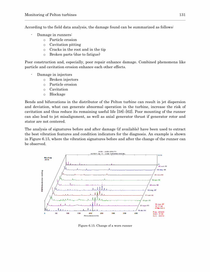
Monitoring of Pelton turbines 131
According to the field data analysis, the damage found can be summarized as follows:
- Damage in runners:
o Particle erosion
o Cavitation pitting
o Cracks in the root and in the tip
o Broken parts (due to fatigue)
Poor construction and, especially, poor repair enhance damage. Combined phenomena like
particle and cavitation erosion enhance each other effects.
- Damage in injectors
o Broken injectors
o Particle erosion
o Cavitation
o Blockage
Bends and bifurcations in the distributor of the Pelton turbine can result in jet dispersion
and deviation, what can generate abnormal operation in the turbine, increase the risk of
cavitation and thus reduce its remaining useful life [58]–[62]. Poor mounting of the runner
can also lead to jet misalignment, as well as axial generator thrust if generator rotor and
stator are not centered.
The analysis of signatures before and after damage (if available) have been used to extract
the best vibration features and condition indicators for the diagnosis. An example is shown
in Figure 6.15, where the vibration signatures before and after the change of the runner can
be observed.
Figure 6.15. Change of a worn runner

132 6.4 Upgrading of the monitoring system
6.4. Upgrading of the monitoring system
The bands usually selected for the monitoring are not refined enough to detect some incipient
problems. One way to upgrade existing monitoring systems is to “follow” the way the runner
vibrates and select the best condition indicators.
The runner vibration modes excited during operation depends on the jet force direction and
on the runner. In Pelton runners, from the rotational reference system perspective, the jet
force is applied to each one of the buckets with a phase shift. In the course of the excitation,
the force on the bucket changes its value and direction. In Figure 6.16, the force variation
induced in a bucket by the jet is shown (taken from [30]). The components of the force 𝐹𝑥, 𝐹𝑦
and𝐹𝑧 correspond to the axial, radial and tangential directions of the wheel, respectively. As
it can be seen in the graph, the most important component is in the perpendicular direction
of the bucket (tangential to the wheel), thus the bending modes are more prone to be excited.
Forces in axial and in radial direction are very small.
Figure 6.16. Distribution of the forces produced by the jet on a bucket (image taken from [30])
Therefore, in normal operating conditions, with the runner and injector in good state and the
jet aligned, the runner vibrates mainly in the tangential direction. With the tangential force,
the tangential modes and other modes with tangential deformation are the ones to be excited.
In an aligned turbine, axial forces should be very small and so the axial deformations and
vibrations. Because the tangential force of the jet depends on the jet discharge, the amplitude
of these modes will increase with load.
Damage and abnormal operation can modify the runner vibration due to the excitation of
other runner modes. Changes in these vibrations can be generated by problems in the jet or
by damage in the runner. Both of them can produce changes in amplitude or in the
distribution of the runner modes.
The most common types of damage change the components of the jet force on the runner.
Axial components of the jet force on the bucket may be not zero if the jet centerline is not
coincident with bucket centerline. An axial force may also appear if the stator magnetic field

Monitoring of Pelton turbines 133
center is not aligned with the rotor magnetic field. In some occasions an axial force are due
to problems in the injector or in the runner.
The analysis of the historic data shows that most of the damage found produces a change in
the jet alignment and jet quality exciting axials modes. A change in jet quality may increase
the turbulent excitation. The effect of jet misalignment can be checked with a simulation of
the harmonic response including the axial component of the jet force.
One possible way to detect these types of damage is by stablishing properly specified spectral
bands after the natural frequencies of rotor and runner has been identified. Spectral bands
around the axial, tangential, rim, radial and other modes can be stablished.
Any change in the state or excitation of the runner will modify these bands. Because the band
energy for the different operating conditions can change with the machine power and with
damage, the mapping of all bands from minimum to maximum power has to be calculated
with ML methods (part 5.6). Mapping for the most common types of damage should be also
included. A history case will be analysed with this method.
The potentiality of each spectral bands levels depend on the machine power but also on the
position and direction. This has been discussed in the last chapters, where the best
monitoring positions have been studied.
6.5. History case
The case reported here corresponds to a Pelton turbine analyzed with a head of 770 m and a
maximum power of 34 MW. It is a horizontal shaft machine composed by a wheel with 22
buckets with a diameter of 1930 mm and one injector.
Periodically, a monitoring analysis is carried out in the machine. Vibrations are measured
on the bearings in the axial and radial directions, in order to monitor the turbine condition.
This procedure allows the surveillance of the machine detecting abnormal vibrational
behavior, and, in some cases, detecting incipient damage. In one of the measurements, the
vibration monitoring system detected an increase in the vibration levels and a change in the
signatures (see Figure 6.17). The RMS velocity values overpassed the alarm level, and the
machine was stopped and inspected. In Figure 6.18, the spectra measured by the vibration
based monitoring system days before, during and after the damage can be observed.

134 6.5 History case
Figure 6.17. Trend plot of the overall vibration values measured in the turbine bearing
Figure 6.18. Frequencies acquired by the monitoring system in the turbine bearing
The inspection of the Pelton wheel showed an important damage in one of the buckets: a
fragment was detached from the outer part of the bucket’s rim. In addition to that, several
buckets showed cracks in the same location. It is important to remark that all damage
appeared in the same side of the wheel. Figure 6.19 shows how the broken bucket looked like
after the failure and the segment of bucket blown off. The analysis of the fragment revealed
that the failure took place due to a fatigue problem. This can be claimed because of the beach
marks, which can easily be identified in the crack.
Fatigue problems appear when a structure is subjected to cyclic loads, which lead to a
concentration of stresses that end up weakening the material. In general, all the studies
reporting Pelton turbine failures evidenced that the main stresses affecting the structure
appear in the bucket’s root.
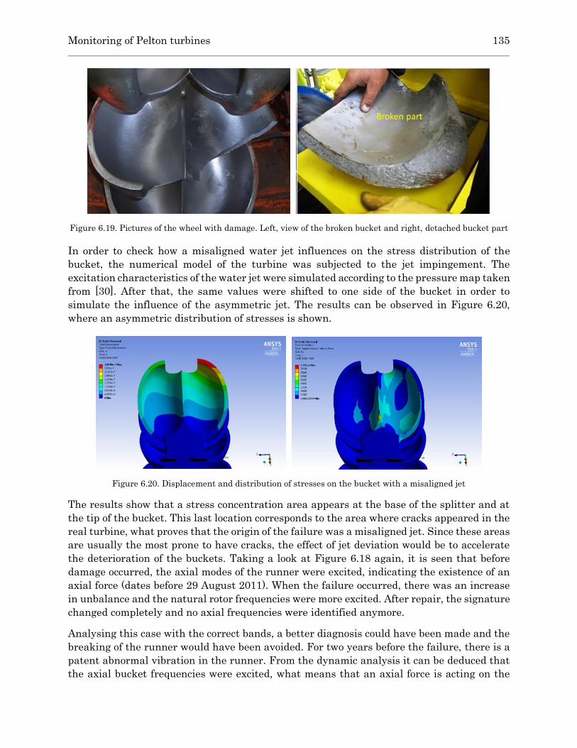
Monitoring of Pelton turbines 135
Figure 6.19. Pictures of the wheel with damage. Left, view of the broken bucket and right, detached bucket part
In order to check how a misaligned water jet influences on the stress distribution of the
bucket, the numerical model of the turbine was subjected to the jet impingement. The
excitation characteristics of the water jet were simulated according to the pressure map taken
from [30]. After that, the same values were shifted to one side of the bucket in order to
simulate the influence of the asymmetric jet. The results can be observed in Figure 6.20,
where an asymmetric distribution of stresses is shown.
Figure 6.20. Displacement and distribution of stresses on the bucket with a misaligned jet
The results show that a stress concentration area appears at the base of the splitter and at
the tip of the bucket. This last location corresponds to the area where cracks appeared in the
real turbine, what proves that the origin of the failure was a misaligned jet. Since these areas
are usually the most prone to have cracks, the effect of jet deviation would be to accelerate
the deterioration of the buckets. Taking a look at Figure 6.18 again, it is seen that before
damage occurred, the axial modes of the runner were excited, indicating the existence of an
axial force (dates before 29 August 2011). When the failure occurred, there was an increase
in unbalance and the natural rotor frequencies were more excited. After repair, the signature
changed completely and no axial frequencies were identified anymore.
Analysing this case with the correct bands, a better diagnosis could have been made and the
breaking of the runner would have been avoided. For two years before the failure, there is a
patent abnormal vibration in the runner. From the dynamic analysis it can be deduced that
the axial bucket frequencies were excited, what means that an axial force is acting on the

136 6.5 History case
runner. This is an abnormal situation, which should have been checked before reaching the
damage level. Under these conditions, as shown in the FEM analysis, the stress distribution
is modified.
In the trend graphs of the next figures, the variation of the selected spectral bands with
abnormal operation and damage can be observed. In Figure 6.21, Figure 6.22 and Figure 6.23
the evolution of the new spectral bands has been represented. At the beginning, there are the
levels with abnormal operation, then the levels with damage and last the levels after repair.
The classical spectral bands like 𝑓𝑓 and 𝑓𝑏 show a large alteration only when the failure
occurs, not before. The same happens with the rotor natural frequencies. Only the axial
runner band shows a big change in abnormal operation before damage took place.
AI techniques can be used to correlate all the bands for a better accuracy in the monitoring.
This can be considered a hybrid approach where physics-based models can be used to
understand the dynamic behavior of the machine. Further processing can be carried out with
new techniques.
With this approach incipient damage like the one indicated in Figure 6.24 could have been
detected and trended.

Monitoring of Pelton turbines 137
Figure 6.21. Variation in the runner 𝑓𝑓 band and 𝑓𝑏 band levels with time
Figure 6.22. Variation in one of the rotor natural frequencies band levels with time
Figure 6.23. Variation in one of the runner axial and tangential frequency band levels with time

138 6.6 Data-driven diagnostic methods
Figure 6.24. Incipient detection
6.6. Data-driven diagnostic methods
Another possibility is to use only data-driven methods. Condition monitoring using machine
learning and cloud solutions is a future application in hydro power plants. Machine learning
is a field of computer science where models are trained on data to predict an output given a
set of input values. These methods train models with historical monitoring data measured in
hydro power plants to predict abnormal operation and damage. If a component breaks down,
the AI methods can identify similar patterns in future. The most common machine learning
methods need data with machine in good condition and with different levels of damage till

Monitoring of Pelton turbines 139
the end of life. Mappings relating features and the damage state have to be created but
hydropower plants are never operated until the end of life. This information is very difficult
to obtain.
Another important disadvantage is that physical cause-effect relationship is not used and
lessons learned analysing what happened to several units may not be good enough to predict
for another unit. Example are Neural Networks (NN).
In Figure 6.25, the three different time-domain signals of the Pelton turbine vibration
discussed before are analyzed here using AI techniques [63]. The signals correspond to the
machine in good condition, with abnormal operation and with damage. Applying
Convolutional Neural Networks, the three situations are learned and identified. The
accuracy of the identification is tested with another segment of the same signal. The
identification is perfect.
Figure 6.25. Data driven approach

140 6.7 Conclusions
6.7. Conclusions
In this chapter the condition monitoring procedures for hydraulic turbines in general
including new trends are introduced.
It follows the application to Pelton turbines, with an analysis of the vibration signatures and
the explanation of actual monitoring procedures.
Once proved that the runner can be monitored from the bearings, the next step has consisted
in knowing the most common types of damage and their symptoms. For that purpose, the
monitoring information and data obtained after more than twenty years of monitoring have
been analyzed. The main types of damage that have occurred in several Pelton turbine units
are described.
A new spectral band distribution is proposed so that the excitation of the different runner
modes can be monitored. An analysis about which of these modes can be excited in normal
an abnormal operation is performed.
The proposed procedure is check with a history case where the evolution of the vibration
signatures with a fatigue induced damage was available. The proposed method is more
sensitive to detect damage and for the diagnostic of damage.

Chapter 7 Conclusions and future work

142 Conclusions and future work
In this thesis the dynamic behavior of horizontal shaft Pelton turbine prototypes has been
investigated. For this purpose, several prototype turbines have been investigated using
numerical models and on-site tests.
Vibrations generated during turbine operation depend on the excitation force produced by
the jet and especially on the modal response of the turbine. In the first part of the thesis, a
detailed analysis of the modal response has been used carried out in a systematic way. First
a single runner suspended and second with the runner attached to the shaft (Chapters 2 and
3)
Modal behavior of Pelton runners
In this chapter, a study of an existing turbine runner (suspended) has been done with a
numerical simulation and with a comprehensive experimental investigation.
First, assuming that the buckets are rigidly connected (to disregard the effect of the disk) the
bucket modes have been studied. In this way, the bucket modes were identified and classified
as axial, tangential and radial. Depending on the phase between the bucket halves, these
modes were in-phase or counter-phase. The first modes found are axial in-phase followed by
tangential in and in counter-phase. After them axial in counter-phase and radials appeared.
Second, the analysis of the complete runner was performed. The results showed that for every
type of basic bucket mode, the runner has several multiples, which are coupled to the modes
of the disk (n nodal diameters). For each group of bucket modes, the frequencies increase
with the number of nodal diameters of the disk. It was noticed that in lower frequencies the
vibration is global to all the runner (behaves like a disk) and in higher frequencies the
vibration is more restricted and is dominated by the vibration of the buckets. In addition,
some bucket modes are more affected by the stiffness of the disk than others are and this
affects the distribution of frequencies. For example, tangential modes gather in a small
frequency range, while axial modes are more spread. The natural frequencies of the whole
runner are lower than the ones obtained with a fixed single bucket.
Because runners are attached to the turbine rotor the influence of this connection is analyzed
in the next chapter.
Modal behavior of Pelton machines
In this chapter, the modal behavior of the whole turbine has been investigated numerically
and experimentally. The main turbine modes were identified with their natural frequencies
and mode shapes.
Modes can be separated into two groups, one as rotor modes and another as runner modes.
Rotor modes cover the lower frequency range from 2,5-3,5 times the rotating frequency to
around 300Hz. Runner modes cover a higher frequency range from 300 to more than 1kHz.

Conclusions and future work 143
The effect of the runner connection to the rotor has been found. The research shows that only
some runner modes are slightly affected because of the added stiffness provided by the
attachment. The first disk modes are affected but the bucket modes not so much.
To check if this behavior was similar in other turbines of different mechanical and hydraulic
design, other turbines were investigated.
The effect of the mechanical design has been studied first. Two runners with the same
hydraulic design but with structural differences were investigated. Tangential modes are the
ones more affected because they are very dependent on the rear bucket structure. However,
the mode distribution and trends are very similar.
The effect of the hydraulic design has also been studied. Significant changes in the modal
behavior have been found. For higher heads the runner is large and the width small. In this
case, the disk dominated modes have lower frequency while the bucket modes have higher
frequencies. The opposite occurs for low head runners.
The method to estimate the diameters and widths of the runner depending on design
operating parameters is proposed. Another important matter is to know if there is any
relationship between the design parameters and the natural frequencies. A correlation has
been found that can be useful for a preliminary estimation of the runner frequency ranges.
In this study the machine was still. When in operation, other effects like the added mass and
centrifugal stresses appear in the runner what may change the modal characteristics. To
determine that, more tests have to be done with the machine in operation.
Because no sensors can be placed on the runner when the machine is in operation, the
feasibility to detect runner vibrations from outside has to be investigated.
Transmissibility of runner vibrations
The transmissibility of runner vibrations to the monitoring positions has been investigated
in this chapter. On-site tests were done in two different turbines.
The investigation shows that all the runner vibrations are transmitted and detected on the
bearings. High coherence values are found between runner and bearing vibrations. Anyway,
the amplitudes seen in the bearing are much smaller than the amplitudes in the runner.
The propagation of the runner natural frequencies to each monitoring position depends on
the mode shapes. The tangential modes are better propagated than axial modes
In general terms, vertical positions have better transmissibility than horizontal positions.
The only exception are the axial counter-phase modes, which are better transmitted to
horizontal positions.

144 Conclusions and future work
In addition, rotor modes and disk-dominated modes are generally better detected from axial
bearing locations, while bucket dominated modes transmit their vibration better to the radial
positions.
It has been proved that the propagation depends on the runner mode shape. A detailed study
to determine which are the best positions to detect each mode was carried out. By doing that,
the best monitoring positions to detect each mode were found. Tangential modes are better
transmitted and better detected in vertical monitoring positions.
So far, the turbine has been studied still. In operation some effects like the centrifugal forces
and the added mass, can modify the natural frequencies. Moreover, the modes excited during
operation have to be determined
For that and with the knowledge obtained with the previous studies, the dynamic behavior
of a Pelton turbine in operation can be performed.
Dynamic behavior of Pelton turbines
The dynamic behavior of two prototype horizontal shaft Pelton turbines in operation has been
investigated. The structural disposition was different, one machine had two bearings at both
sides of the generator and the other three bearings. A simultaneous measurement of
vibrations, noise and strains on the shaft was performed. The sensors were located on
bearings and shaft. The operating conditions were taken from the Scada system. First the
start-up and second the steady operating conditions were analyzed.
The study of the start-up transient gives important information. In the beginning of the start-
up, when the runner is still, vibrations are generated by the excitation of the runner natural
frequencies from the initial impact of the jet. The tangential modes and rim modes are
especially excited by the impact of the water jet on the buckets. In this moment acceleration
amplitudes are larger than when the machine is at full load.
The onboard system showed that the transmission from shaft to the bearing varies with the
runner mode. In addition, strain gauge proved to be capable of detecting runner modes,
especially tangential modes.
After that moment, when the runner increases the rotating speed, the main vibration
amplitudes are due to the match between the blade passing frequency fb and the natural
frequencies of the rotor. The vibration amplitude depends on the mode shape and damping
characteristics. The amplitudes of the more global mode shapes where all the rotor masses
are deformed have the lowest amplitude. The response in the axial direction also depends on
the mode shape characteristics.
The strain measurement indicates that the torsion stress fluctuates at the rotation frequency
with low amplitudes and at the blade passing frequency. The maximum amplitude occurs
when the blade passing frequency equals the torsion natural frequency.
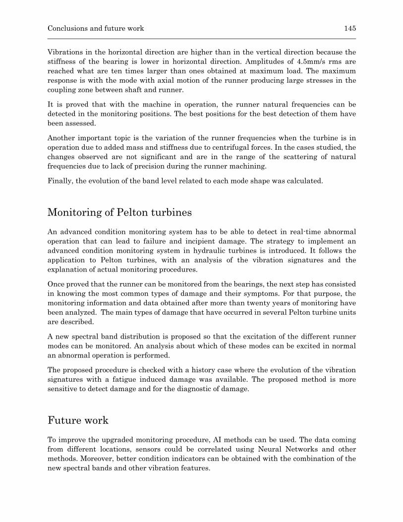
Conclusions and future work 145
Vibrations in the horizontal direction are higher than in the vertical direction because the
stiffness of the bearing is lower in horizontal direction. Amplitudes of 4.5mm/s rms are
reached what are ten times larger than ones obtained at maximum load. The maximum
response is with the mode with axial motion of the runner producing large stresses in the
coupling zone between shaft and runner.
It is proved that with the machine in operation, the runner natural frequencies can be
detected in the monitoring positions. The best positions for the best detection of them have
been assessed.
Another important topic is the variation of the runner frequencies when the turbine is in
operation due to added mass and stiffness due to centrifugal forces. In the cases studied, the
changes observed are not significant and are in the range of the scattering of natural
frequencies due to lack of precision during the runner machining.
Finally, the evolution of the band level related to each mode shape was calculated.
Monitoring of Pelton turbines
An advanced condition monitoring system has to be able to detect in real-time abnormal
operation that can lead to failure and incipient damage. The strategy to implement an
advanced condition monitoring system in hydraulic turbines is introduced. It follows the
application to Pelton turbines, with an analysis of the vibration signatures and the
explanation of actual monitoring procedures.
Once proved that the runner can be monitored from the bearings, the next step has consisted
in knowing the most common types of damage and their symptoms. For that purpose, the
monitoring information and data obtained after more than twenty years of monitoring have
been analyzed. The main types of damage that have occurred in several Pelton turbine units
are described.
A new spectral band distribution is proposed so that the excitation of the different runner
modes can be monitored. An analysis about which of these modes can be excited in normal
an abnormal operation is performed.
The proposed procedure is checked with a history case where the evolution of the vibration
signatures with a fatigue induced damage was available. The proposed method is more
sensitive to detect damage and for the diagnostic of damage.
Future work
To improve the upgraded monitoring procedure, AI methods can be used. The data coming
from different locations, sensors could be correlated using Neural Networks and other
methods. Moreover, better condition indicators can be obtained with the combination of the
new spectral bands and other vibration features.

146 Conclusions and future work
The data of continuous monitoring could be used for the mapping of the condition indicators
in different operating conditions. Historical data can be used to map the change of these
conditions indicators with the most common types of damage.
Regarding the transmission of vibrations from the runner to te monitoring positions, other
on-site tests should be done with an on-board system measuring runner vibrations so that
the changes in the FRF between runner and bearing could be improved.

References
[1] L. Gaudard and F. Romerio, “The future of hydropower in Europe: Interconnecting
climate, markets and policies,” Environ. Sci. Policy, pp. 1–10, 2013.
[2] “International Renewable Energy Agency (IRENA).” [Online]. Available:
https://www.irena.org/hydropower. [Accessed: 10-Jul-2019].
[3] Z. Zhang, Pelton turbines. 2016.
[4] H. Keck, G. Vullioud, and P. Joye, “Commissioning and Operation Experience with the
World’s largest Pelton turbines Bieudron,” pp. 1–16, 2004.
[5] A. Bezinge and P. Loth, “Cleuson-Dixence extension sets world records,” Hydropower Dams, no. March, pp. 29–34, 1994.
[6] A. A. Fulton, “Present Tendencies in Water Turbine Machinery,” Proc. Inst. Mech. Eng., vol. 135, no. 1, pp. 387–444, 1937.
[7] A. B. Winterbottom, “Cracking of Bucket Lugs in Pelton Turbines,” vol. 127, 1951.
[8] M. Nechleba, Hydraulic Turbines. Their Design and Equipment. 1957.
[9] H. Grein, R. Angehrn, M. Lorenz, and A. Bezinge, “Inspection periods of Pelton
runners.”
[10] H. Brekke, “State of the art in Pelton turbine design,” Hydropower Dams, no. March,
pp. 21–28, 1994.
[11] M. Bjerke, H. Brekke, and K. I. Berg, “Modern design and manufacturing of multijet
Pelton turbines,” in Proceedings of the 15th IAHR Symposium on Hydraulic Machinery and Systems, 1990, vol. 2.
[12] H. Brekke, “A discussion on operational problems,” Proc. 24th Symp. Hydraul. Mach. Syst., no. 7026, pp. 1–12.
[13] J. Mañanés, A. Mirasso, and A. Antunez, “Manufacture of the Pelton runners of
Pykara, India,” Hydropower Dams, no. 6, pp. 58–59, 1999.
[14] J. Vesely, J. Mikulasek, and P. Vesely, “Modern technologies for producing Pelton
runners,” Hydropower Dams, no. 2, pp. 113–117, 2006.
[15] J. Veselý and M. Varner, “A Case Study of Upgrading of 62.5MW Pelton Turbine.”
[16] R. Angehrn, H. Grein, W. Keiser, and H. Kloter, “The maintenance of Pelton turbine
runners,” Hydropower Dams, no. March, pp. 35–40, 1994.
[17] J. C. Chávez, J. A. Valencia, G. A. Jaramillo, J. J. Coronado, and S. A. Rodríguez,
“Failure analysis of a Pelton impeller,” Eng. Fail. Anal., vol. 48, pp. 297–307, 2015.
[18] L. Chapuis and K. Froschl, “Optimized fabrication of Pelton turbine runners,”
International Journal on Hydropower and Dams, vol. 5, no. 2. pp. 30–32, 1998.
[19] C. Calderaro and J. Mañanes, “Recent trends in the manufacture of Pelton runners,”

148 References
Hydropower Dams, pp. 109–110, 1997.
[20] A. Kalberer and M. Krause, “A review of experience with MicroCast Pelton wheels,”
Hydropower Dams, no. 1, pp. 22–24, 1996.
[21] F. Linet, G. Rossi, B. Michel, and P.-Y. Lowys, “Hooped runner design offers
advantages for Pelton units,” Hydropower Dams, no. 6, pp. 60–62, 1999.
[22] G. C. Chaudhari and S. P. Shah, “GT2011-46052,” pp. 1–9, 2016.
[23] M. Sick, H. Keck, G. Vullioud, and E. Parkinson, “New Challenges in Pelton Research,”
in Proceedings oh Hydro 2000 Conference, 2000.
[24] J. Schmied, T. Weiss, and R. Angehrn, “Detuning of Pelton Runners,” Proc. 7th IFToMM Conf. Rotor Dyn., no. September, pp. 25–28, 2006.
[25] M. Sick, W. Michler, T. Weiss, and H. Keck, “Recent developments in the dynamic
analysis of water turbines,” Proc. Inst. Mech. Eng. Part A J. Power Energy, vol. 223,
no. 4, pp. 415–427, 2009.
[26] R. Mack and C. Probst, “Evaluation of the dynamic behavior of a Pelton runner based
on strain gauge measurements,” IOP Conf. Ser. Earth Environ. Sci., 2016.
[27] R. Angehrn and M. Dubas, “Experimental stress analysis on a 260MW Pelton runner,”
in Proceedings of the 11th IAHR Symposium, 1982.
[28] R. Angehrn, J. Rettich, and C. Schärer, “Pelton runner design based on measured
unsteady pressure distributions in the bucket,” Hydropower Dams, no. 6, pp. 53–57,
1999.
[29] B. Zoppé, C. Pellone, T. Maitre, and P. Leroy, “Flow Analysis Inside a Pelton Turbine
Bucket,” J. Turbomach., vol. 128, no. 3, p. 500, 2006.
[30] S. Kvicinsky, “Méthode d’analyse des écoulements 3D à surface libre: application aux
turbines Pelton,” École Polytechnique Fédérale de Lausanne, 2002.
[31] F. Avellan, P. Dupont, S. Kvicinsky, L. Chapuis, E. Parkinson, and G. Vullioud, “Flow
calculations in Pelton turbines. Part 2 : Free Surface Flows,” in Proceedings of the 19th IAHR Symposium on Hydraulic Machinery and Systems, 1998, vol. 1.
[32] A. Perrig, “Hydrodynamics of the free surface flow in Pelton turbine buckets,” ÉCOLE
POLYTECHNIQUE FÉDÉRALE DE LAUSANNE, 2007.
[33] H. Brekke, “A review on dynamic problems in Francis and Pelton Turbines,” IOP Conf. Ser. Earth Environ. Sci., vol. 22, pp. 1–10, 2014.
[34] M. Sanvito, L. Coscarelli, E. Pesatori, G. Turozzi, and P. Pennacchi, “A New Method
for the Dynamic Analysis of Pelton Runners Using CFD/FEM Interaction,” Proc. ASME 2009 Int. Des. Eng. Tech. Conf. Comput. Inf. Eng. Conf., pp. 1–5, 2009.
[35] E. Pesatori, G. Turozzi, P. Pennacchi, and A. Tosi, “Dynamic Investigation on a Pelton
Runner: FEM Calculations and Experimental Results,” Proc. ASME 2007 Int. Des. Eng. Tech. Conf. Comput. Inf. Eng. Conf., pp. 3–7, 2007.
[36] P. Dörfler, M. Sick, and A. Coutu, Flow-Induced Pulsation and Vibration in

References 149
Hydroelectric Machinery. Springer, 2013.
[37] A. Karakolcu, J. Erhard, and B. Wittwer, “Best practice in rehabilitation of Pelton
turbines as applied at Vermuntwerk M5,” Proc. 17th Int. Semin. Hydropower Plants,
pp. 1–20, 2012.
[38] E. Egusquiza, Comportament dinàmic de màquines hidràuliques. 2003.
[39] F. De Siervo and A. Lugaresi, “Modern trends in selecting and designing Pelton
turbines,” Water Power & Dam Construction, vol. pp. 40–48, 1978.
[40] P. Heckbert, “Fourier Transforms and the Fast Fourier Transform (FFT) Algorithm,”
Notes Comput. Graph., vol. 3, no. 2, pp. 15–463, 1995.
[41] T. Irvine, “An Introduction to Frequency Response Functions.” pp. 1–29, 2000.
[42] M. A. Kramer, “An introduction to field analysis techniques: the power spectrum and
coherence,” Soc. Neurosci., pp. 18–25, 2013.
[43] P. Loth, H. Sprysl, and G. Ebi, “Bearing stiffness determination through vibration
analysis of shaft line of Bieudron Hydro Powerplant,” Int. J. Hydro Power Dams, pp.
427–447, 1998.
[44] M. Egusquiza, “Study of the axial modes of Pelton turbines,” 2017.
[45] B. Thapa and H. Brekke, “Effect of sand particle size and surface curvature in erosion
of hydraulic turbine,” 22nd IAHR Symp. Hydraul. Mach. Syst. Stock. Sweden, June 29 - July 2, 2004, vol. 1, no. 11, pp. 1–11, 2004.
[46] M. K. Padhy and R. P. Saini, “A review on silt erosion in hydro turbines,” Renew. Sustain. Energy Rev., vol. 12, no. 7, pp. 1974–1987, 2008.
[47] M. K. Padhy and R. P. Saini, “Study of silt erosion mechanism in Pelton turbine
buckets,” Energy, vol. 39, no. 1, pp. 286–293, 2012.
[48] T. R. Bajracharya, B. Acharya, C. B. Joshi, R. P. Saini, and O. G. Dahlhaug, “Sand
erosion of Pelton turbine nozzles and buckets: A case study of Chilime Hydropower
Plant,” Wear, vol. 264, no. 3–4, pp. 177–184, 2008.
[49] O. G. Dahlhaug and T. Nielsen, “Efficiency loss in Pelton buckets due to sediment
erosion,” in Proceedings of the 23rd IAHR Symposium on Hydraulic Machinery and Systems, 2006, vol. 1, no. October, pp. 2–7.
[50] A. K. Rai, A. Kumar, and T. Staubli, “Hydro-abrasive erosion in Pelton buckets :
Classification and field study,” Wear, vol. 393, no. August, pp. 8–20, 2017.
[51] H. Grein, “Cavitation Pitting and Rain Erosion on Pelton Turbines,” in Proceedings of the 15th IAHR Symposium on Hydraulic Machinery and Systems, 1990, vol. 1.
[52] M. Pradel, “Pelton runner manufacture from forged stainless steel,” Hydropower Dams, no. January, pp. 25–26, 1995.
[53] K. Stevanovic, “Damage of the Pelton turbine wheel,” Proc. Int. Conf. CSHS03, pp.
219–226, 2003.
[54] E. Egusquiza, C. Valero, A. Estévez, A. Guardo, and M. Coussirat, “Failures due to

150 References
ingested bodies in hydraulic turbines,” Eng. Fail. Anal., 2011.
[55] X. Liu, Y. Luo, and Z. Wang, “A review on fatigue damage mechanism in hydro
turbines,” Renew. Sustain. Energy Rev., vol. 54, no. FEBRUARY, pp. 1–14, 2016.
[56] M. Mione and G. Mazza, “Repairing cast Pelton runners: Problems and modern
solutions,” International Journal on Hydropower and Dams, vol. 6, no. 6. pp. 63–65,
1999.
[57] A. Panthee, B. Thapa, and H. P. Neopane, “Quality control in welding repair of Pelton
runner,” Renew. Energy, vol. 79, no. 1, pp. 96–102, 2015.
[58] Z. Zhang and M. Casey, “Experimental studies of the jet of a Pelton turbine,” Proc. Inst. Mech. Eng. Part A J. Power Energy, vol. 221, no. 8, pp. 1181–1192, 2007.
[59] E. Parkinson, R. Lestriez, and L. Chapuis, “Flow calculations in Pelton Turbines - Part
1 Repartitor and injector numerical analysis,” Proc. 19th IAHR Symp. Hydraul. Mach. Syst., pp. 285–293, 1998.
[60] M. Peron, E. Parkinson, L. Geppert, and T. Staubli, “Importance of jet quality on Pelton
efficiency and cavitation,” in International Conference on Hydraulic Efficiency Measurements, 2008, pp. 1–9.
[61] T. Staubli et al., “Jet quality and Pelton efficiency,” Hydro 2009 Prog. - Potential – Plans, Lyon, Fr., 2009.
[62] B. W. Solemslie and O. G. Dahlhaug, “Studying the effects of jet alignment in Pelton
units,” Int. J. Hydropower Dams, vol. 22, no. 3, pp. 78–83, 2015.
[63] W. Zhao and M. Egusquiza, “Application of CNN to Pelton machine diagnostics,” 2019.
Related Documents


![Current Technology if Radial-Inflow Turbines fir Compressible ...the "Pelton," "Francis," and "Kaplan" [4]. Pelton turbines have a special geometry which has no true counterpart in](https://static.cupdf.com/doc/110x72/6099c308eda602790f724e3b/current-technology-if-radial-inflow-turbines-fir-compressible-the-pelton.jpg)