Faculty of Sciences Department of Astrophysics, Geophysics and Oceanography Study of supernovae and massive stars and prospects with the 4m International Liquid Mirror Telescope Brajesh Supervisors: Dr. Shashi Bhushan Pandey Prof. Jean Surdej A thesis submitted in fulfilment of the requirements for the degree of Doctor of Philosophy (Sciences) in the Extragalactic Astrophysics and Space Observations group November 2014

Welcome message from author
This document is posted to help you gain knowledge. Please leave a comment to let me know what you think about it! Share it to your friends and learn new things together.
Transcript
University of Li
ege
Faculty of Sciences
Department of Astrophysics, Geophysics and Oceanography
Study of supernovae and massivestars and prospects with the 4m
International Liquid MirrorTelescope
Brajesh Kumar
Supervisors:
Dr. Shashi Bhushan Pandey
Prof. Jean Surdej
A thesis submitted in fulfilment of the requirementsfor the degree of Doctor of Philosophy (Sciences)
in the
Extragalactic Astrophysics and Space Observations group
November 2014

Universit
e de Li
ege
Faculte des Sciences
Department d’Astrophysique, Geophysique et Oceanographie
Etude de supernovae et d’etoilesmassives et perspectives d’avenir
dans le cadre du projetinternational du telescope a miroir
liquide de 4m
Brajesh Kumar
Promoteurs:
Dr. Shashi Bhushan Pandey
Prof. Jean Surdej
Dissertation presentee en vue de l’obtention du grade de Docteur enSciences
au sein du groupe AEOS (Astrophysique Extragalactique etObservations Spatiales)
Novembre 2014

Members of the Jury – Prof. S. Habraken (President)Prof. S. Covino (OAB)Dr. E. Gosset (ULg)Prof. P. Hickson (UBC)Prof. Gregor Rauw (ULg)Dr. S. B. Pandey (ARIES)Prof. J. Surdej (ULg)

To,
Maaee, Babuji
and my family

Abstract
Massive stars are the progenitors of the most energetic explosions in the Universe
such as core-collapse supernovae (CCSNe) and gamma ray bursts. During their life
time they follow various evolutionary phases (e.g. supergiant, luminous blue variable
andWolf-Rayet). They strongly influence their environments through their energetic
ionization radiation and powerful stellar winds. Furthermore, the formation of low-
and intermediate-mass stars are also being regulated by them.
The Carina nebula region, which hosts a large population of massive stars and
several young star clusters, provides an ideal target for studying the feedback of
massive stars. In this thesis, we investigated a wide field (32′ × 31′) region located
in the west of the Carina nebula and centered on the massive binary WR 22. For our
study, we used new optical photometry (UBVRI Hα), along with some low resolution
spectroscopy, archival near infra-red (2MASS), and X-ray (Chandra, XMM-Newton)
data. We estimated several parameters such as reddening, reddening law, etc. and
also identified young stellar objects located in the region under study (Kumar et al.,
2014b).
Among the various types of CCSNe, Type IIb are recognized with their typical
observational properties. Some of them show clear indication of double peaks in
their light curves. The spectral features of these SNe show a transition between
Type II and Type Ib/c events at early and later epochs, respectively. It has been
noticed that the occurrence of these events is not common in volume limited surveys.
In this thesis we have studied the properties of the light curve and spectral evolution
of the Type IIb supernova 2011fu. The observational properties of this object show
resemblance to those of SN 1993J with a possible signature of the adiabatic cooling
phase (Kumar et al., 2013).
When light passes through the expanding ejecta of the SNe, it retains information
about the orientation of the ejected layers. In general, CCSNe exhibit a significant
level of polarization during various phases of their evolution at different wavelengths.
We have investigated the broad band polarimetric properties of a Type II plateau
SN 2012aw and compared it with other well-studied CCSNe of similar kinds (Kumar
et al., 2014a).
In the framework of the present thesis, we have also contributed to the devel-
opment of the 4m International Liquid Mirror Telescope (ILMT) project which is
a joint collaborative effort among different universities and research institutes in

Belgium, India, Canada and Poland. We performed various experiments including
the spin casting of the primary mirror, optical quality tests of the mercury surface,
mylar film experiments, etc. The possible scientific capabilities and future contri-
butions of this telescope are also discussed. We propose our plans to identify the
transients (specially supernovae) with the ILMT and their further follow-up scheme.
The installation of the ILMT will start very soon at the Devasthal observatory,
ARIES Nainital, India.
viii
Resume
Les etoiles massives sont a l’origine des explosions les plus energetiques ren-
contrees dans l’Univers, comme les supernovae resultant de l’effondrement de l’etoile
centrale (en anglais ≪ core-collapse supernovae≫, dont l’acronyme est CCSNe) et
les sursauts gamma. Au cours de leur existence, elles suivent differentes phases
d’evolution comme la phase de supergeante, d’etoile variable lumineuse bleue et/ou
d’etoile de type Wolf-Rayet. Les etoiles massives influencent fortement leur environ-
nement grace a leur prodigieux rayonnement ionisant et leur puissant vent stellaire.
Elles peuvent, en outre, regir la formation d’etoiles a faible masse et d’etoiles de
masse intermediaire.
La region de la nebuleuse de la Carene, qui contient une importante population
d’etoiles massives ainsi que plusieurs jeunes amas d’etoiles, constitue une cible ideale
pour etudier les effets causes par la presence d’etoiles massives. Dans cette these,
nous avons etudie un grand champ (32′ × 31′) situe a l’ouest de la nebuleuse de la
Carene et centre sur l’etoile binaire massive WR 22. Au cours de notre etude, nous
avons utilise de nouvelles donnees photometriques dans le domaine visible (UBVRI
et Hα), de la spectroscopie a basse resolution ainsi que des donnees d’archives qui
couvrent des domaines de longueur d’onde allant du proche infra-rouge (2MASS)
aux rayons X (Chandra, XMM-Newton). Nous avons estime les valeurs de plusieurs
parametres physiques tels que le rougissement interstellaire, la loi de rougissement,
etc. et egalement identifie des jeunes objets stellaires situes dans la region etudiee
(Kumar et al., 2014b).
Parmi les differents types de CCSNe, les supernovae de type IIb sont reconnaiss-
ables grace a des traits observationnels distincts. Certaines d’entre elles presentent
clairement la presence d’un double pic dans leur courbe de lumiere. Les car-
acteristiques spectrales de ces supernovae montrent une transition entre le type
II ayant lieu dans les periodes les plus anciennes et les evenements de type Ib/c
se deroulant a des epoques plus tardives. On a remarque que la frequence de ces
evenements n’est pas elevee dans un survey limite en volume. Dans le present tra-
vail, nous avons etudie les proprietes de la courbe de lumiere et l’evolution spectrale
de la supernova 2011fu de Type IIb. Les caracteristiques observationnelles de cet
objet montrent une forte ressemblance a celles de SN 1993J, avec une signature
possible de la phase de refroidissement adiabatique (Kumar et al., 2013).
Lorsque la lumiare passe au travers des ejectas en expansion de la supernova, elle
conserve les informations relatives a l’orientation des couches ejectees. En general,
les CCSNe presentent un niveau eleve de polarisation au cours des differentes phases
de leur evolution et a differentes longueurs d’onde. Nous avons ainsi etudie les pro-
prietes polarimetriques a larges bandes de la supernova SN 2012aw de type IIP, dont
la courbe de lumiere montre un plateau, et compare celles-ci avec d’autres CCSNe
du meme type qui ont precedemment fait l’objet d’une etude detaillee (Kumar et al.,
2014a).
Dans le cadre de cette these, nous avons egalement contribue a l’elaboration du
projet du telescope a miroir liquide international (ILMT, en enanglais International
Liquid Mirror Telescope) de 4m de diametre qui est le fruit d’une collaboration con-
jointe entre differentes universites et instituts de recherche situes en Belgique, en
Inde, au Canada et en Pologne. Nous avons realise diverses experiences, y compris
le coulage d’une resine par centrifugation du miroir primaire, et nous avons aussi
effectue des tests de qualite optique de la surface du mercure et des experiences avec
un film Mylar. Les performances attendues de ce telescope sont discutees. Nous
proposons notamment une strategie observationnelle en vue d’identifier au moyen
du ILMT des phenomenes astrophysiques transitoires tels que les explosions de su-
pernovae et leur suivi observationnel avec d’autres grands telescopes et instruments.
L’installation du ILMT va bientot commencer a l’observatoire de Devasthal
(ARIES) situe dans l’etat de l’Uttarakhand, en Inde.
x
Acknowledgments
A collaboration between ARIES (Aryabhatta Research Institute of Observational
Sciences), India and University of Liege, Belgium provided me a great opportunity
to fulfill the need of the present thesis. During my stay at both of these places
I received enormous help and support from several people. Here I would like to
acknowledge them.
First of all my heartfelt gratitudes and sincere thanks to my thesis supervisors,
Prof. Jean Surdej and Dr. Shashi Bhushan Pandey. Since I started my career as a
researcher, Dr. Shashi has always been encouraging and motivating me. I improved
my scientific capabilities with the help of fruitful discussions with him throughout
the tenure of my PhD. Since my association with the ILMT project, Prof. Jean
has helped me not only through his scientific intellectualities but also as a guardian
during my stay in Belgium. He provided me full freedom and support to work and
establish new collaborations. I appreciate your financial supports at different stages
of my work. I sincerely thank Prof. Ram Sagar for being with us over many years as
the ARIES director and providing great contribution to develop ARIES as a premier
institution in the area of astrophysics and atmospheric research. Your motivating
words and scientific temperaments will always inspire me.
I acknowledge the members of my thesis committee, for having accepted to read
and evaluate this PhD thesis.
I wish to pay my special thanks to my collaborators who have been involved in
various affairs of my research work. Thank you Prof. P. Hickson and Prof. J. P.
Swings for your precious advice for the development of the ILMT. I am grateful to
Prof. G. C. Anupama and Dr. D. K. Sahu for providing data from HCT. Prof. G.
Rauw, Dr. E. Gosset, Prof. V. V. Sokolov, Dr. A. S. Moskvitin, Dr. J. Vinko, Dr.
J. Gorosabel and Dr. J. Manfroid are highly acknowledged for the fruitful scientific
discussions.
I feel grateful to the Academic Committee of ARIES for their support, arranging
lectures and discussion. I acknowledge the staff members of the 104 cm and 130
cm telescopes for their assistance during the observations. I also thank the ARIES
library, computer, administrative, electrical and mechanical sections for their help
in my research activities.
I acknowledge the support and suggestions from Dr. Wahab Uddin and Dr. A.
K. Pandey. I thank Drs. Brijesh, Ramakant, Saurabh, Kuntal, Biman, Snehlata,

Jeewan, Hum Chand, Maheswar and Manish for their ever helpful attitude and dis-
cussions in various academic matters. I am also thankful to senior scientists and
engineers at ARIES who helped me from time to time. Thanks to the supernova
research group members at ARIES – Rupak, Subhash and Vijay for their support in
observations and useful scientific discussions. I appreciate the observers at ARIES
who provided their valuable observing time to support the transient follow-up pro-
grams.
It would not have been possible to complete my work without the help, support
and encouragement of my colleagues and friends. I am lucky to have their company.
Thank you Eswar for your continuous motivation, a lot of things I have learnt
from you. I am indebted to Ram Kesh for his company and discussions on various
topics. Arti, Manash, Himali, Jessy, Neelam, Sanjeev and Chavi are acknowledged
for their timely help in any academic problems. It was enjoyable to discuss various
scientific and non-scientific topics with Sumana, Akash, Narendra, Bindu, Ravi,
Devesh, Hema, Tapaswini, Krishna, Archana, Sumit, Pradip, Rajiv, Piyush, Raman
and Jai. I also thank research fellows Abhishek, Neha, Subhajeet, Parveen, Arti,
Aditi, Aabha, Mridweeka, Mukesh and other researchers for their nice company in
ARIES.
My stay at Liege could not have been easy and productive without the support
and help of my friends, colleagues and well-wishers. I am indebted to Francois,
Arnaud and Ludovic for their nice company and sharing various technical aspects
of ILMT. Thank you Andrii and Olga for your helping nature, I still remember the
very first evening in ULg when I forgot the way to return to my residing place but
luckily found you. I spent fun filled time with Yassine, Tatyana, Chloi, Chandra,
Balloo, Shubhayan and Renuka in Liege. Thanks to all of you.
It is impossible for me to forget the help and support of Sylvia and Denise.
Whenever I faced any kind of problem either academic or residential, they solved it
quickly and made my life easier. I gratefully acknowledge the association of Anna
with us always. I felt homely by talking with her. Thank you Catalina for inducing
me to learn French.
Most of all, I express my gratitude to my parents whose blessings, love and con-
stant support made me to complete this work. Thank youMaaee and Babuji, I could
have not completed my thesis work without your motivation and encouragement. I
am very lucky to have my brothers Devesh, Yogendra and sister Urmila who have
taken care of my parents as well as my children. Their belief and trust encouraged
xii

me to do my work with freedom. I am thankful to my wife Suman who has been
a constant source of support in my life. You have been my true companion and a
constructive force. Dear Prakriti and Anant, I am sorry for not being with you on
most of the occasions but I love you and carry the memories of the time we spend
together. Thank you both for bringing so much joy in my life. I am grateful to all
my near and dear ones who directly or indirectly helped me to complete the present
work. And finally, I thank Almighty for his blessings to make this work reality for
me!!
I sincerely acknowledge ARIES for the financial support, utilizing the observa-
tional facilities for the transient observations during my PhD thesis. I also thankfully
acknowledge the University of Liege for the financial support, providing invaluable
data and fruitful involvement in the ILMT project.
xiii

NOTATIONS AND ABBREVIATIONS
The notations and abbreviations which have been used in this thesis are collected
here for a quick reference. All these notations and abbreviations have also been
explained on their first appearance in the text.
Notations
A Angstrom (unit of wavelength)
α Right ascension′, arcmin Arcminute′′, arcsec Arcsecond
cm Centimeter
Dec., δ Declination, deg Degree
∆m15 Decline in magnitude for the first 15 days after maximum
e− Electron
Aλ Total attenuation at wavelength λ
RV Ratio of total to selective extinction
E(B − V ) Colour excess in B − V (reddening)
Fig. Figure
GHz Giga Hertz
Hz Hertz (unit of frequency)
H0 Hubble parameter
ISPHG Interstellar polarization due to host galactic dust
h, hr Hour
hrs Hours
ISPMW Milky Way interstellar polarization
J2000 Epoch of observation
km Kilometer
λ Wavelength
kpc Kiloparsec (unit of distance)
M⊙ Mass of the Sun
Mpc Megaparsec
m Meter
mm Millimeter
µm Micrometer
xv
milliarcsec Milliarcsecond
min Minutes
Ωm Matter density of the Universe
ΩΛ Vacuum energy density
PR Polarization in R-band
PA Polarization angle
Pmean Mean polarization efficiency
pc Parsec (unit of distance)
Ref. References
RA Right Ascension
R⊙ Radius of the Sun
rms, σ Root mean square
σPRUncertainty in the polarization in R-band
σθR Uncertainty in the polarization angle in R-band
s, sec Second
Sect. Section
θR Polarization angle in R-band
UBV RIJHKHα Apparent magnitudes in U,B,V,R,I,J,H,K,Hα bands
W Watt
yr Year
z Redshift
Abbreviations
ADU Analog to Digital Unit
AEOS Astrophysique Extragalactique et Observations Spatiales
AGN Active Galactic Nucleus
ARIES Aryabhatta Research Institute of observational sciencES
ASAS-SN All-Sky Automated Survey for Supernovae
CBET Central Bureau for Electronic Telegrams
CCD Charge Coupled Device
CCSNe Core Collapse Supernovae
xvi
CF Completeness Factor (CF)
CMD Colour Magnitude Diagram
CNC Carina Nebula Complex
CRTS Catalina Real-Time Transient Survey
CSM Circumstellar Medium
CSS Catalina Sky Survey
CTTS Classical T Tauri Star
DAOPHOT Dominion Astrophysical Observatory Photometry (software)
DFOT Devasthal Fast Optical Telescope
DOT Devasthal Optical Telescope
DST Department of Science and Technology, Govt. of India
FITS Flexible Image Transport System
FWHM Full Width at Half Maximum
ESO European Southern Observatory
GELATO GEneric cLAssification TOol
HCT Himalayan Chandra Telescope
HST Hubble Space Telescope
iPTF intermediate Palomar Transient Factory
IAO Indian Institute of Astrophysics
IAU International Astronomical Union
IAUC International Astronomical Union Circular
IIA Indian Institute of Astrophysics
ILMT International Liquid Mirror Telescope
IMF Initial Mass Function ISM Interstellar Medium
IRAF Image Reduction and Analysis Facility (software)
JD Julian Date
KLF K-band Luminosity Function
LC Light Curve
LIDAR LIght Detection and RAnging
LM Liquid Mirror
LMT Liquid Mirror Telescope
LOSS Lick Observatory Supernova Search
LSST Large Synoptic Survey Telescope
LZT Large Zenithal Telescope
2MASS Two Micron All Sky Survey
xvii
MIDAS Munich Image and Data Analysis System
MS Main Sequence
MST Minimal Spanning Tree
NASA National Aeronautics and Space Administration
NED NASA Extragalactic Database
NGC New General Catalog
NIR Near-infrared
NOAO National Optical Astronomy Observatories
NODO NASA Orbital Debris Observatory
NOT Nordic Optical Telescope
NTT New Technology Telescope
Pan-STARRS Panoramic Survey Telescope & Rapid Response System
PLC Polarization Light Curve
PMS Pre-main Sequence
PPS Precision Precast Solutions
PSF Point Spread Function
PTF Palomar Transient Factory
QE Quantum Efficiency
QSO Quasi Stellar Object
ROTSE Robotic Optical Transient Search Experiment
SCP Supernova Cosmology Project
SDSS Sloan Digital Sky Survey
SI Spectral Instruments
SN, SNe Supernova, Supernovae
SNLS Supernova Legacy Survey
STRESS Southern inTermediate Redshift ESO Supernova Search
SNID Supernova Identification
ST Sampurnanand Telescope
TCD Two Colour Diagram
USNO United States Naval Observatory
UT Universal Time
UVOT Ultra-Violet Optical Telescope
VLT Very Large Telescope
WISE Wide-Field Infrared Survey Explorer
WFI Wide Field Imager
xviii

WR Wolf-Rayet
WTTS Weak line T Tauri Star
XMM X-ray Multi-Mirror Mission
XRT X-ray Telescope
YSO Young Stellar Object
ZAMS Zero Age Main Sequence
ZTF Zwicky Transient Facility
xix

Contents
Nomenclature xli
I Introduction 1
1 Massive stars, supernovae and liquid mirror telescopes 3
1.1 Massive stars . . . . . . . . . . . . . . . . . . . . . . . . . . . . . . . 3
1.1.1 Evolutionary phases of massive stars . . . . . . . . . . . . . . 4
1.1.1.1 Supergiants (SGs) . . . . . . . . . . . . . . . . . . . 5
1.1.1.2 Luminous blue variables (LBVs) . . . . . . . . . . . 6
1.1.1.3 WR stars . . . . . . . . . . . . . . . . . . . . . . . . 6
1.1.2 Massive stars forming regions and their environments . . . . . 10
1.2 Core collapse supernovae . . . . . . . . . . . . . . . . . . . . . . . . . 11
1.2.1 Observational features and classifications of CCSNe . . . . . . 12
1.2.2 Explosion mechanisms of CCSNe . . . . . . . . . . . . . . . . 18
1.2.3 Polarization properties of CCSNe . . . . . . . . . . . . . . . . 21
1.2.4 Supernova rate: observational and theoretical overview . . . . 23
1.3 Liquid mirror telescopes (LMTs) . . . . . . . . . . . . . . . . . . . . 25
1.3.1 LMT history and recent progress . . . . . . . . . . . . . . . . 26
1.3.2 Basic principle . . . . . . . . . . . . . . . . . . . . . . . . . . 27
1.3.3 Usefulness of LMTs . . . . . . . . . . . . . . . . . . . . . . . . 29
1.3.4 Major LMT observing facilities and their scientific contributions 31
II Massive stars and supernovae 37
2 Study of the Carina nebula massive star forming region 39
2.1 Introduction . . . . . . . . . . . . . . . . . . . . . . . . . . . . . . . . 39
2.2 Observations and data analysis . . . . . . . . . . . . . . . . . . . . . 42
xxi
CONTENTS
2.2.1 Optical photometry . . . . . . . . . . . . . . . . . . . . . . . . 42
2.2.2 Completeness of the data . . . . . . . . . . . . . . . . . . . . . 44
2.2.3 Spectroscopy . . . . . . . . . . . . . . . . . . . . . . . . . . . 45
2.2.4 Archival data: 2MASS . . . . . . . . . . . . . . . . . . . . . . 45
2.3 Basic parameters . . . . . . . . . . . . . . . . . . . . . . . . . . . . . 45
2.3.1 Reddening . . . . . . . . . . . . . . . . . . . . . . . . . . . . . 45
2.3.2 Reddening law . . . . . . . . . . . . . . . . . . . . . . . . . . 47
2.3.3 Distance . . . . . . . . . . . . . . . . . . . . . . . . . . . . . . 50
2.4 Results . . . . . . . . . . . . . . . . . . . . . . . . . . . . . . . . . . . 50
2.4.1 Spectroscopically identified sources . . . . . . . . . . . . . . . 50
2.4.2 YSOs identification . . . . . . . . . . . . . . . . . . . . . . . . 52
2.4.2.1 On the basis of Hα emission . . . . . . . . . . . . . . 53
2.4.2.2 On the basis of IR excess . . . . . . . . . . . . . . . 54
2.4.2.3 On the basis of X-ray emission . . . . . . . . . . . . 59
2.4.3 Age and mass of YSOs . . . . . . . . . . . . . . . . . . . . . . 63
2.4.3.1 Using NIR CMD . . . . . . . . . . . . . . . . . . . . 63
2.4.3.2 Using optical CMD . . . . . . . . . . . . . . . . . . . 64
2.4.4 Initial mass function . . . . . . . . . . . . . . . . . . . . . . . 68
2.4.5 K-band luminosity function . . . . . . . . . . . . . . . . . . . 70
2.5 Discussion: star formation scenario in the CrW region . . . . . . . . . 72
2.6 Summary and conclusions . . . . . . . . . . . . . . . . . . . . . . . . 79
3 CCSNe, progenitors: the Type IIb supernova 2011fu 83
3.1 Introduction . . . . . . . . . . . . . . . . . . . . . . . . . . . . . . . . 83
3.2 Observations and Data Analysis . . . . . . . . . . . . . . . . . . . . . 85
3.2.1 Optical Photometry . . . . . . . . . . . . . . . . . . . . . . . . 86
3.2.2 Spectroscopic observations . . . . . . . . . . . . . . . . . . . . 88
3.3 Multi-band light curves of SN 2011fu . . . . . . . . . . . . . . . . . . 91
3.3.1 Explosion epoch of SN 2011fu . . . . . . . . . . . . . . . . . . 91
3.3.2 Light curve analysis . . . . . . . . . . . . . . . . . . . . . . . . 92
3.3.3 Colour evolution and reddening towards SN 2011fu . . . . . . 94
3.3.4 Comparison of the absolute magnitudes . . . . . . . . . . . . . 96
3.4 Bolometric light curve . . . . . . . . . . . . . . . . . . . . . . . . . . 97
3.4.1 Construction of the bolometric light curve . . . . . . . . . . . 97
3.4.2 Bolometric light curve modelling . . . . . . . . . . . . . . . . 98
3.5 Spectral analysis . . . . . . . . . . . . . . . . . . . . . . . . . . . . . 102
xxii
CONTENTS
3.5.1 Comparison between observed and synthetic spectra . . . . . . 102
3.5.2 Velocity of the pseudo-photosphere . . . . . . . . . . . . . . . 104
3.5.3 Hydrogen and the 6200A absorption feature . . . . . . . . . . 104
3.5.4 Other ions . . . . . . . . . . . . . . . . . . . . . . . . . . . . . 107
3.5.5 Results of spectral modelling . . . . . . . . . . . . . . . . . . . 107
3.6 Metallicity-Brightness comparison of host galaxies . . . . . . . . . . . 108
3.7 Conclusions . . . . . . . . . . . . . . . . . . . . . . . . . . . . . . . . 110
4 Broad Band Polarimetric study of the Type IIP SN 2012aw 113
4.1 Introduction . . . . . . . . . . . . . . . . . . . . . . . . . . . . . . . . 113
4.1.1 SN 2012aw . . . . . . . . . . . . . . . . . . . . . . . . . . . . 115
4.2 Observations and data reduction . . . . . . . . . . . . . . . . . . . . . 118
4.3 Estimation of the intrinsic polarization . . . . . . . . . . . . . . . . . 120
4.3.1 Interstellar polarization due to the Milky Way (ISPMW) . . . . 120
4.3.2 Interstellar polarization due to the host galactic dust (ISPHG) 123
4.4 Discussion . . . . . . . . . . . . . . . . . . . . . . . . . . . . . . . . . 128
4.4.1 Polarization light curve (PLC) analysis . . . . . . . . . . . . . 128
4.4.2 Q and U parameters . . . . . . . . . . . . . . . . . . . . . . . 129
4.4.3 Comparison with other Type IIP events . . . . . . . . . . . . 130
4.5 Conclusions . . . . . . . . . . . . . . . . . . . . . . . . . . . . . . . . 133
III The 4m International Liquid Mirror Telescope and
search for supernovae 135
5 The 4m International Liquid Mirror Telescope project 137
5.1 Introduction . . . . . . . . . . . . . . . . . . . . . . . . . . . . . . . . 137
5.2 Major components of the ILMT . . . . . . . . . . . . . . . . . . . . . 141
5.2.1 Air bearing and air supply system . . . . . . . . . . . . . . . . 141
5.2.2 Primary mirror . . . . . . . . . . . . . . . . . . . . . . . . . . 144
5.2.3 Support structure and safety pillars . . . . . . . . . . . . . . . 145
5.2.4 CCD camera and Time Delay Integration . . . . . . . . . . . . 146
5.2.5 Filters . . . . . . . . . . . . . . . . . . . . . . . . . . . . . . . 149
5.2.6 Optical corrector . . . . . . . . . . . . . . . . . . . . . . . . . 150
5.3 Science with the ILMT . . . . . . . . . . . . . . . . . . . . . . . . . . 151
5.4 Essential ILMT equipment . . . . . . . . . . . . . . . . . . . . . . . . 153
5.4.1 Air compressor and air receiver . . . . . . . . . . . . . . . . . 153
xxiii
CONTENTS
5.4.2 Air membrane dryer and dew point sensor . . . . . . . . . . . 156
6 Preliminary tests with the 4m ILMT 157
6.1 Container reinforcement . . . . . . . . . . . . . . . . . . . . . . . . . 157
6.2 Primary mirror spin casting . . . . . . . . . . . . . . . . . . . . . . . 159
6.2.1 Initial preparations . . . . . . . . . . . . . . . . . . . . . . . . 159
6.2.2 Final preparations . . . . . . . . . . . . . . . . . . . . . . . . 161
6.3 Mercury tests: constructing the liquid mirror . . . . . . . . . . . . . . 165
6.3.1 Mercury as a reflecting liquid . . . . . . . . . . . . . . . . . . 165
6.3.2 Mercury exposure limit . . . . . . . . . . . . . . . . . . . . . . 166
6.3.3 Important safety equipments . . . . . . . . . . . . . . . . . . . 168
6.3.4 ILMT surface quality test . . . . . . . . . . . . . . . . . . . . 172
6.4 Mylar film experiment . . . . . . . . . . . . . . . . . . . . . . . . . . 173
6.4.1 Experimental set-up and analysis . . . . . . . . . . . . . . . . 175
6.5 TDI mode observations and preliminary data reduction . . . . . . . . 176
7 Supernovae detection in the 4m ILMT strip 181
7.1 Introduction . . . . . . . . . . . . . . . . . . . . . . . . . . . . . . . . 181
7.2 Throughput and limiting magnitude of a telescope . . . . . . . . . . . 185
7.3 Area and accessible volume of the ILMT strip . . . . . . . . . . . . . 186
7.4 Estimation of the supernova rate . . . . . . . . . . . . . . . . . . . . 189
7.4.1 Supernovae observations with the ILMT and follow-up scheme 191
7.4.1.1 TDI mode imaging . . . . . . . . . . . . . . . . . . . 193
7.4.1.2 Image subtraction . . . . . . . . . . . . . . . . . . . 194
7.4.1.3 Transient detection and possible contamination . . . 195
7.4.1.4 Further observations . . . . . . . . . . . . . . . . . . 195
7.5 Summary . . . . . . . . . . . . . . . . . . . . . . . . . . . . . . . . . 200
IV Conclusions and future prospects 201
8 Conclusions and future prospects 203
Appendix 213
References 247
xxiv
List of Figures
1.1 Hertzsprung-Russell diagram showing the main sequence tracks for 1,
5 and 10 solar mass stars. Additionally, regions for specific evolution-
ary phases are indicated. Image credit http://www.atnf.csiro.au. 4
1.2 A sketch of the upper HR diagram with various evolutionary phases
of massive stars. Possible tracks of the progenitors of SN 1987A,
SN 1993J and Cas A are also indicated. Figure taken from Smith
(2010). . . . . . . . . . . . . . . . . . . . . . . . . . . . . . . . . . . . 7
1.3 Classification scheme of the various types of supernovae based on the
early optical spectra and light curve properties. . . . . . . . . . . . . 14
1.4 Schematic light curves for SNe of Type Ia, Ib, IIP, IIL and the peculiar
SN 1987A, taken from Wheeler & Harkness (1990). The light curve
for SNe Ib includes SNe Ic as well, and represents an average. . . . . 14
1.5 Spectral evolution of different types of SNe at various epochs – near
maxima, 3 weeks and one year after maxima (from, Turatto, 2003) . . 15
1.6 Sequence of events during the collapse of a typical stellar core to a
nascent neutron star. It begins with a massive star with an ‘onion-
skin’ structure, goes through white-dwarf core implosion, to core
bounce and shock-wave formation, to the protoneutron-star stage
before explosion, and finally to the cooling and isolated-neutron-star
stage after explosion. Figure reproduced from Burrows (2000). . . . . 19
1.7 Different types of supernovae (upper panel) and their remnants (lower
panel) generated from non rotating massive single stars having dif-
ferent initial mass and metallicity. The figures are taken from Heger
et al. (2003a). The sharp lines are the boundaries, segregating the
outcomes of different kinds of catastrophe generated from the progen-
itors of different masses and metallicities. A strip of pair-instability
supernovae is also shown that leaves no remnant. . . . . . . . . . . . 20
xxv
LIST OF FIGURES
1.8 Sketch of polarization production in supernovae. Panel A: Zero net
polarization is produced in case of a spherical supernova atmosphere.
For a non-spherical atmosphere, there will be some level of polariza-
tion (panel: B). The uneven blocked light due to clumps of material
may also produce a net supernova polarization (panel: C). Image is
reproduced from Leonard (2007). . . . . . . . . . . . . . . . . . . . . 22
1.9 Upper panel: Number of detected SNe per year. The discovery year
of SN 1987A is marked with a dashed line. The fraction of bright
SNe, which have a magnitude at maximum V < 15, is indicated by
the hatched area. The figure is from Lennarz et al. (2012). Lower
left and right panels: percentage of CCSNe of a particular type in
the respective studies of Eldridge et al. (2013) and Smith et al. (2011). 24
1.10 Illustration of the basic principle of a liquid mirror telescope. The
parabolic shape of the rotating fluid results from the combined ef-
fect of the centrifugal acceleration (horizontal arrow) and the grav-
itational one (vertical arrow). A CCD camera inserted at the focal
plane will image the stellar objects passing over the zenith. Figure
reproduced from Finet (2013). . . . . . . . . . . . . . . . . . . . . . . 28
1.11 Left panel: Image of UBC/Laval 2.7m LMT, taken from http://
www.astro.ubc.ca/lmt/lm/. Right panel: Narrow band TDI image
(∼19’×19’) of a field at 15h 29m +49 14’ (1950) obtained with a
single scan by this telescope. North is up and east is to the left. The
bright star is SAO 045572. The effective integration time is 129 sec.
This image has been taken from Hickson et al. (1994). . . . . . . . . . 32
1.12 Left panel: Image of the primary mirror NODO telescope. Image is
from http://www.astro.ubc.ca/lmt/Nodo. Right image: an image
taken with the NODO. The field is 5’ × 7’. R.A. = 12h 08m, Dec. =
33 00’ (J2000.0). Image credit Cabanac et al. (1998). . . . . . . . . . 32
1.13 Left panel: LZT primary mirror filled with mercury. Right panel:
Colour composite image (100 sec exposure in g, r and i filters) ob-
tained with the LZT. Images taken from http://www.astro.ubc.
ca/ lmt/lzt/index.html. . . . . . . . . . . . . . . . . . . . . . . . . 33
xxvi
LIST OF FIGURES
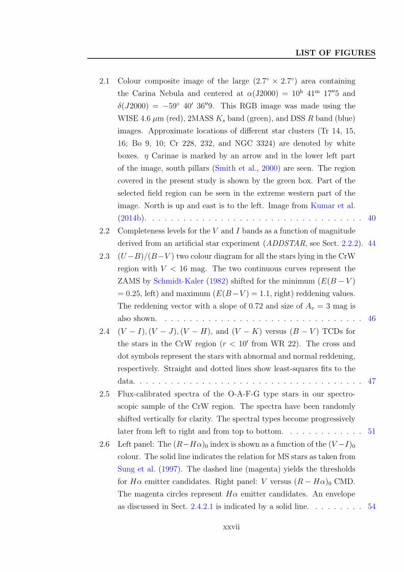
2.1 Colour composite image of the large (2.7 × 2.7) area containing
the Carina Nebula and centered at α(J2000) = 10h 41m 17′′5 and
δ(J2000) = −59 40′ 36′′9. This RGB image was made using the
WISE 4.6 µm (red), 2MASS Ks band (green), and DSS R band (blue)
images. Approximate locations of different star clusters (Tr 14, 15,
16; Bo 9, 10; Cr 228, 232, and NGC 3324) are denoted by white
boxes. η Carinae is marked by an arrow and in the lower left part
of the image, south pillars (Smith et al., 2000) are seen. The region
covered in the present study is shown by the green box. Part of the
selected field region can be seen in the extreme western part of the
image. North is up and east is to the left. Image from Kumar et al.
(2014b). . . . . . . . . . . . . . . . . . . . . . . . . . . . . . . . . . . 40
2.2 Completeness levels for the V and I bands as a function of magnitude
derived from an artificial star experiment (ADDSTAR, see Sect. 2.2.2). 44
2.3 (U−B)/(B−V ) two colour diagram for all the stars lying in the CrW
region with V < 16 mag. The two continuous curves represent the
ZAMS by Schmidt-Kaler (1982) shifted for the minimum (E(B − V )
= 0.25, left) and maximum (E(B−V ) = 1.1, right) reddening values.
The reddening vector with a slope of 0.72 and size of Av = 3 mag is
also shown. . . . . . . . . . . . . . . . . . . . . . . . . . . . . . . . . 46
2.4 (V − I), (V − J), (V − H), and (V − K) versus (B − V ) TCDs for
the stars in the CrW region (r < 10′ from WR 22). The cross and
dot symbols represent the stars with abnormal and normal reddening,
respectively. Straight and dotted lines show least-squares fits to the
data. . . . . . . . . . . . . . . . . . . . . . . . . . . . . . . . . . . . . 47
2.5 Flux-calibrated spectra of the O-A-F-G type stars in our spectro-
scopic sample of the CrW region. The spectra have been randomly
shifted vertically for clarity. The spectral types become progressively
later from left to right and from top to bottom. . . . . . . . . . . . . 51
2.6 Left panel: The (R−Hα)0 index is shown as a function of the (V −I)0
colour. The solid line indicates the relation for MS stars as taken from
Sung et al. (1997). The dashed line (magenta) yields the thresholds
for Hα emitter candidates. Right panel: V versus (R−Hα)0 CMD.
The magenta circles represent Hα emitter candidates. An envelope
as discussed in Sect. 2.4.2.1 is indicated by a solid line. . . . . . . . . 54
xxvii
LIST OF FIGURES
2.7 Column density distribution of the molecular cloud in our field of
view, as derived from the near-infrared reddening of stars. The lowest
contour corresponds to Av = 3.4, the step size of the contours is 0.2.
The RA and Dec are in degrees. . . . . . . . . . . . . . . . . . . . . . 56
2.8 K0/(H − K)0 CMD for (a) stars in the CrW region, (b) stars in
the field region and (c) same stars as in panel (a) along with identi-
fied probable NIR-excess stars. The blue dashed line represents the
envelope of field CMD, whereas the red solid line demarcates the
distribution of IR excess sources from MS stars. . . . . . . . . . . . . 57
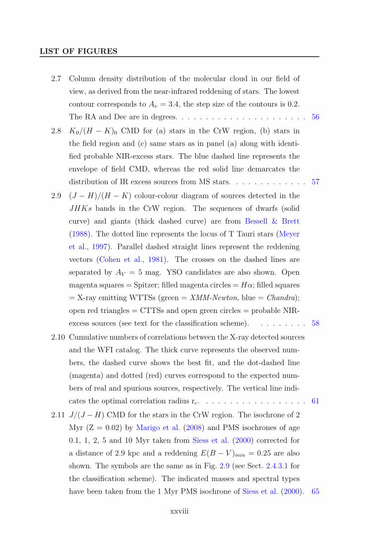
2.9 (J − H)/(H − K) colour-colour diagram of sources detected in the
JHKs bands in the CrW region. The sequences of dwarfs (solid
curve) and giants (thick dashed curve) are from Bessell & Brett
(1988). The dotted line represents the locus of T Tauri stars (Meyer
et al., 1997). Parallel dashed straight lines represent the reddening
vectors (Cohen et al., 1981). The crosses on the dashed lines are
separated by AV = 5 mag. YSO candidates are also shown. Open
magenta squares = Spitzer; filled magenta circles =Hα; filled squares
= X-ray emitting WTTSs (green = XMM-Newton, blue = Chandra);
open red triangles = CTTSs and open green circles = probable NIR-
excess sources (see text for the classification scheme). . . . . . . . . 58
2.10 Cumulative numbers of correlations between the X-ray detected sources
and the WFI catalog. The thick curve represents the observed num-
bers, the dashed curve shows the best fit, and the dot-dashed line
(magenta) and dotted (red) curves correspond to the expected num-
bers of real and spurious sources, respectively. The vertical line indi-
cates the optimal correlation radius rc. . . . . . . . . . . . . . . . . . 61
2.11 J/(J −H) CMD for the stars in the CrW region. The isochrone of 2
Myr (Z = 0.02) by Marigo et al. (2008) and PMS isochrones of age
0.1, 1, 2, 5 and 10 Myr taken from Siess et al. (2000) corrected for
a distance of 2.9 kpc and a reddening E(B − V )min = 0.25 are also
shown. The symbols are the same as in Fig. 2.9 (see Sect. 2.4.3.1 for
the classification scheme). The indicated masses and spectral types
have been taken from the 1 Myr PMS isochrone of Siess et al. (2000). 65
xxviii
LIST OF FIGURES
2.12 V/(V −I) CMD for all the detected YSOs (symbols as in Fig. 2.9, see
Sect. 2.4.2.2 for details). The isochrone for 2 Myr by Marigo et al.
(2008) (continuous line) and PMS isochrones for 1, 2, 5, and 10 Myr
by Siess et al. (2000) (dashed lines) are also shown. All the isochrones
are corrected for a distance of 2.9 kpc and reddening E(B−V ) = 0.25.
The horizontal line with an arrow corresponds to the completeness
limit of the observations. . . . . . . . . . . . . . . . . . . . . . . . . . 66
2.13 Histograms showing the distribution of YSO candidates ages (left
panel) and masses (right panel) in the observed CrW region. The
green and red histograms are for the estimated ages and masses of
YSOs assuming a distance of 2.9 kpc and 2.3 kpc, respectively. The
error bars along the ordinates represent ±√N Poisson errors. . . . . 67
2.14 Plot of the mass function in the CrW region. Log Φ represents
logN(log m). The error bars represent ±√N errors. The solid line
shows a least-squares fit over the entire mass range 0.5 < M/M⊙ <
4.8. Open and filled circles represent the points below and above the
completeness limit of our data, respectively. . . . . . . . . . . . . . . 69
2.15 Panel (a) Comparison between the observed KLF in the reference field
(red filled circles) and the simulated KLF from star counts modeling
(blue filled triangles). If the star counts represent the number N of
stars in a bin, the associated error bars are ±√N . The KLF slope
(α, see Sect. 2.4.5) of the reference field (solid line) is 0.34 ± 0.01.
The simulated model (dashed line) also gives the same value of slope
(0.34 ± 0.02). Panel (b) The KLF for the CrW region (filled red
circles) and the simulated star counts (blue filled triangles). In the
magnitude range 10.5 − 14.25, the best-fit KLF slope (α) for the
CrW region (solid line) is 0.31± 0.01, whereas for the model (dashed
line), after taking extinction into account, it comes out to be 0.36±0.02. 71
xxix
LIST OF FIGURES
2.16 Spatial distributions of different classes of YSOs. Various symbols are
overlaid on the WISE 4.6 µm image. The filled square symbols rep-
resent X-ray identified sources (XMM-Newton bigger green, Chandra
sources small blue). Open magenta squares, open red triangles, filled
magenta circles, and open green circles are Spitzer-identified YSOs,
CTTSs, Hα emission stars, and probable NIR-excess YSOs, respec-
tively. Purple star symbols are Herschel YSO sources. The abscissae
and the ordinates represent RA and Dec, respectively for the J2000
epoch. . . . . . . . . . . . . . . . . . . . . . . . . . . . . . . . . . . . 73
2.17 Cumulative distribution of the MST branch lengths. In panel (a), the
solid lines represent the linear fits to the points smaller and larger
than the chosen critical branch length. The critical radius is shown
by a vertical line. Panel (b) is the histogram of the MST branch
lengths for the YSOs in the CrW region (see text). . . . . . . . . . . 75
2.18 Top: Minimal spanning tree of the YSOs overplotted on a colour
composite image of the CrW region (WISE 22 µm (red), Hα band
(green), and V band (blue) images). WR 22 is situated in the center.
The white circles connected with dotted lines, and black circles con-
nected with solid lines are the branches that are larger and smaller
than the basic critical length, respectively. The identified ten cluster
cores are encircled with yellow colour and labeled with A to J. Bot-
tom: Two zoomed images of YSO cores, C and E, are shown in the
lower left and right panels, respectively (see text for detail). . . . . . 77
2.19 Spatial distribution of the optically identified YSO candidates in the
CrW region. The size of the symbols represents the age of the YSO
candidate, i.e. bigger the size younger the YSO is. Various colours
represent YSO candidates identified using different schemes (Spitzer
- orange, Hα - purple, CTTS - red, Chandra sources - black, XMM-
Newton - blue, and IR excess - green). . . . . . . . . . . . . . . . . . 79
3.1 V -band image of the SN 2011fu field around the galaxy UGC 01626,
observed on 2011 November 16 with the 1-m ST, India. The SN is
marked with a black arrow. The reference standard stars used for
calibration are marked with numbers 1-8. On this image, north is up
and east is to the left. . . . . . . . . . . . . . . . . . . . . . . . . . . 85
xxx
LIST OF FIGURES
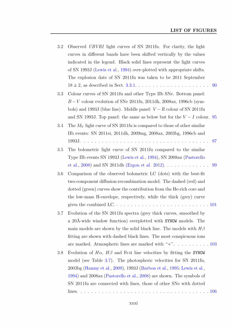
3.2 Observed UBVRI light curves of SN 2011fu. For clarity, the light
curves in different bands have been shifted vertically by the values
indicated in the legend. Black solid lines represent the light curves
of SN 1993J (Lewis et al., 1994) over-plotted with appropriate shifts.
The explosion date of SN 2011fu was taken to be 2011 September
18± 2, as described in Sect. 3.3.1. . . . . . . . . . . . . . . . . . . . . 90
3.3 Colour curves of SN 2011fu and other Type IIb SNe. Bottom panel:
B−V colour evolution of SNe 2011fu, 2011dh, 2008ax, 1996cb (sym-
bols) and 1993J (blue line). Middle panel: V −R colour of SN 2011fu
and SN 1993J. Top panel: the same as below but for the V − I colour. 95
3.4 TheMV light curve of SN 2011fu is compared to those of other similar
IIb events: SN 2011ei, 2011dh, 2009mg, 2008ax, 2003bg, 1996cb and
1993J. . . . . . . . . . . . . . . . . . . . . . . . . . . . . . . . . . . . 97
3.5 The bolometric light curve of SN 2011fu compared to the similar
Type IIb events SN 1993J (Lewis et al., 1994), SN 2008ax (Pastorello
et al., 2008) and SN 2011dh (Ergon et al. 2012). . . . . . . . . . . . . 99
3.6 Comparison of the observed bolometric LC (dots) with the best-fit
two-component diffusion-recombination model. The dashed (red) and
dotted (green) curves show the contribution from the He-rich core and
the low-mass H-envelope, respectively, while the thick (grey) curve
gives the combined LC. . . . . . . . . . . . . . . . . . . . . . . . . . . 101
3.7 Evolution of the SN 2011fu spectra (grey thick curves, smoothed by
a 20A-wide window function) overplotted with SYNOW models. The
main models are shown by the solid black line. The models with Hβ
fitting are shown with dashed black lines. The most conspicuous ions
are marked. Atmospheric lines are marked with “+”. . . . . . . . . . 103
3.8 Evolution of Hα, Hβ and Fe ii line velocities by fitting the SYNOW
model (see Table 3.7). The photospheric velocities for SN 2011fu,
2003bg (Hamuy et al., 2009), 1993J (Barbon et al., 1995; Lewis et al.,
1994) and 2008ax (Pastorello et al., 2008) are shown. The symbols of
SN 2011fu are connected with lines, those of other SNe with dotted
lines. . . . . . . . . . . . . . . . . . . . . . . . . . . . . . . . . . . . . 106
xxxi
LIST OF FIGURES
3.9 Metallicity-luminosity relation for various types of SNe host galax-
ies. The tiny dots belong to all galaxies used by Prieto et al. (2008)
(This catalog is based on SDSS DR4 Adelman-McCarthy et al., 2006,
database). Red squares refere to Type II, stars to Type Ib/c and black
dots to Type IIb SNe, respectively. The analytic relations collected
from several papers (see text) are also over-plotted. The SN 2011fu
host metallicity is denoted by a black triangle. . . . . . . . . . . . . . 109
4.1 R-band image of the SN 2012aw field around the host galaxy M95,
observed on 2012 April 17 using AIMPOL with the 1.04 m ST, India.
Each object has two images. The ordinary and extra-ordinary images
of SN 2012aw and its host galaxy are labeled as o and e, respectively.
The galaxy is marked with a white arrow and the SN is located 60′′
west, 115′′ south of the center of the M95 galaxy. The North and
East directions are also indicated. . . . . . . . . . . . . . . . . . . . . 116
4.2 Left panel: Optical layout of the AIMPOL (image reproduced from
Rautela et al. (2004)). Right panel: AIMPOL mounted on the 1.04-m
ST telescope. . . . . . . . . . . . . . . . . . . . . . . . . . . . . . . . 119
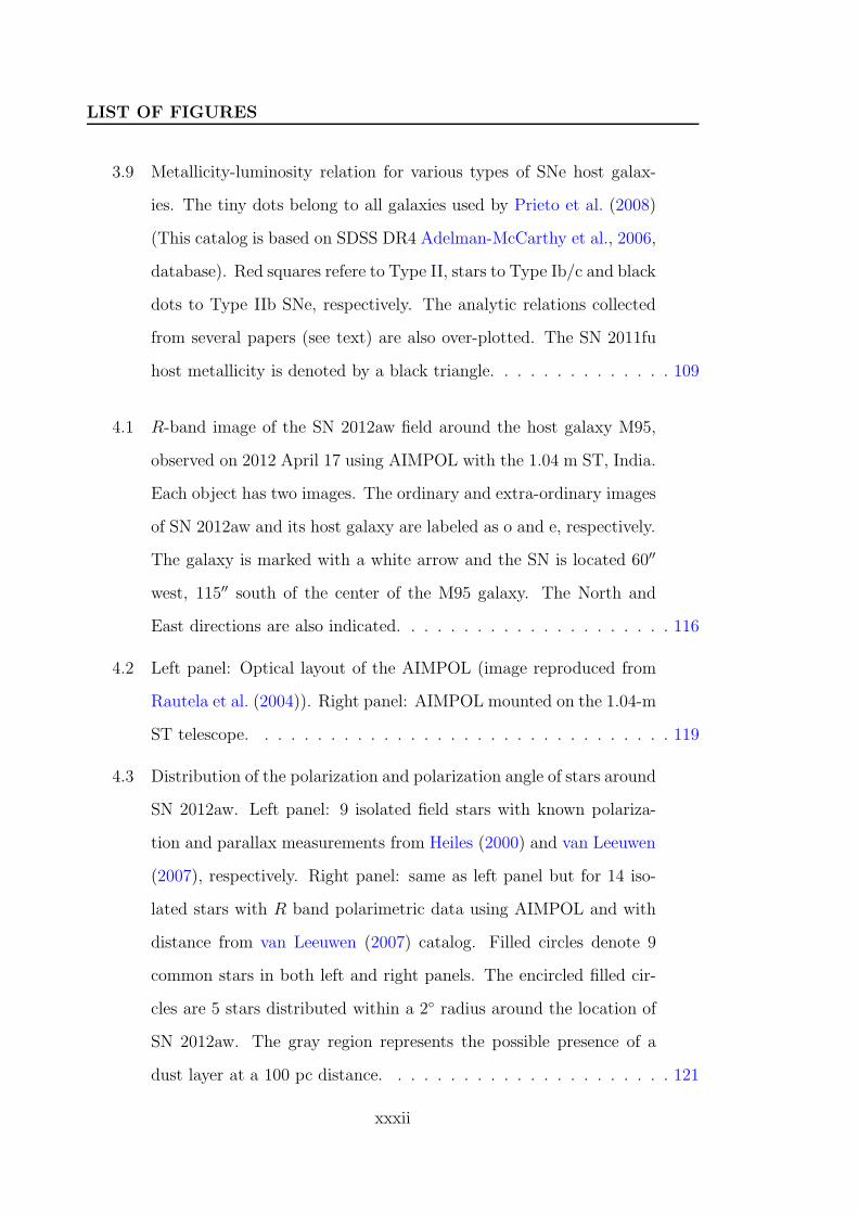
4.3 Distribution of the polarization and polarization angle of stars around
SN 2012aw. Left panel: 9 isolated field stars with known polariza-
tion and parallax measurements from Heiles (2000) and van Leeuwen
(2007), respectively. Right panel: same as left panel but for 14 iso-
lated stars with R band polarimetric data using AIMPOL and with
distance from van Leeuwen (2007) catalog. Filled circles denote 9
common stars in both left and right panels. The encircled filled cir-
cles are 5 stars distributed within a 2 radius around the location of
SN 2012aw. The gray region represents the possible presence of a
dust layer at a 100 pc distance. . . . . . . . . . . . . . . . . . . . . . 121
xxxii
LIST OF FIGURES
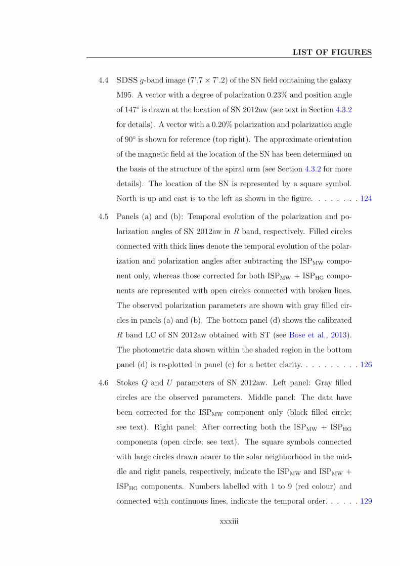
4.4 SDSS g-band image (7’.7 × 7’.2) of the SN field containing the galaxy
M95. A vector with a degree of polarization 0.23% and position angle
of 147 is drawn at the location of SN 2012aw (see text in Section 4.3.2
for details). A vector with a 0.20% polarization and polarization angle
of 90 is shown for reference (top right). The approximate orientation
of the magnetic field at the location of the SN has been determined on
the basis of the structure of the spiral arm (see Section 4.3.2 for more
details). The location of the SN is represented by a square symbol.
North is up and east is to the left as shown in the figure. . . . . . . . 124
4.5 Panels (a) and (b): Temporal evolution of the polarization and po-
larization angles of SN 2012aw in R band, respectively. Filled circles
connected with thick lines denote the temporal evolution of the polar-
ization and polarization angles after subtracting the ISPMW compo-
nent only, whereas those corrected for both ISPMW + ISPHG compo-
nents are represented with open circles connected with broken lines.
The observed polarization parameters are shown with gray filled cir-
cles in panels (a) and (b). The bottom panel (d) shows the calibrated
R band LC of SN 2012aw obtained with ST (see Bose et al., 2013).
The photometric data shown within the shaded region in the bottom
panel (d) is re-plotted in panel (c) for a better clarity. . . . . . . . . . 126
4.6 Stokes Q and U parameters of SN 2012aw. Left panel: Gray filled
circles are the observed parameters. Middle panel: The data have
been corrected for the ISPMW component only (black filled circle;
see text). Right panel: After correcting both the ISPMW + ISPHG
components (open circle; see text). The square symbols connected
with large circles drawn nearer to the solar neighborhood in the mid-
dle and right panels, respectively, indicate the ISPMW and ISPMW +
ISPHG components. Numbers labelled with 1 to 9 (red colour) and
connected with continuous lines, indicate the temporal order. . . . . . 129
xxxiii
LIST OF FIGURES
4.7 Comparison of the polarization and polarization angle values of SN 2012aw
with those of other Type IIP SNe: SN 1987A, SN 1999em, SN 2004dj,
SN 2005af, SN 2006ov, SN 2007aa and SN 2008bk. The upper and
lower panels show the degree of polarization and polarization angle,
respectively. All values are intrinsic to a particular SN and symbols
used in both panels are same. Thick and broken lines denote ISPMW
and both ISPMW + ISPHG subtracted components, respectively for
SN 2012aw. . . . . . . . . . . . . . . . . . . . . . . . . . . . . . . . . 131
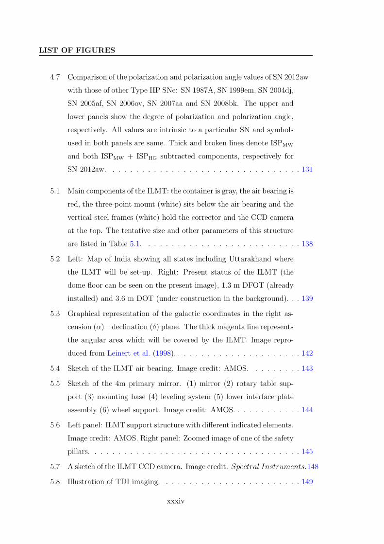
5.1 Main components of the ILMT: the container is gray, the air bearing is
red, the three-point mount (white) sits below the air bearing and the
vertical steel frames (white) hold the corrector and the CCD camera
at the top. The tentative size and other parameters of this structure
are listed in Table 5.1. . . . . . . . . . . . . . . . . . . . . . . . . . . 138
5.2 Left: Map of India showing all states including Uttarakhand where
the ILMT will be set-up. Right: Present status of the ILMT (the
dome floor can be seen on the present image), 1.3 m DFOT (already
installed) and 3.6 m DOT (under construction in the background). . . 139
5.3 Graphical representation of the galactic coordinates in the right as-
cension (α) – declination (δ) plane. The thick magenta line represents
the angular area which will be covered by the ILMT. Image repro-
duced from Leinert et al. (1998). . . . . . . . . . . . . . . . . . . . . . 142
5.4 Sketch of the ILMT air bearing. Image credit: AMOS. . . . . . . . . 143
5.5 Sketch of the 4m primary mirror. (1) mirror (2) rotary table sup-
port (3) mounting base (4) leveling system (5) lower interface plate
assembly (6) wheel support. Image credit: AMOS. . . . . . . . . . . . 144
5.6 Left panel: ILMT support structure with different indicated elements.
Image credit: AMOS. Right panel: Zoomed image of one of the safety
pillars. . . . . . . . . . . . . . . . . . . . . . . . . . . . . . . . . . . . 145
5.7 A sketch of the ILMT CCD camera. Image credit: Spectral Instruments.148
5.8 Illustration of TDI imaging. . . . . . . . . . . . . . . . . . . . . . . . 149
xxxiv
LIST OF FIGURES
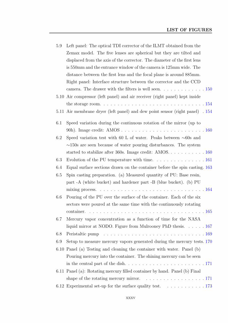
5.9 Left panel: The optical TDI corrector of the ILMT obtained from the
Zemax model. The five lenses are spherical but they are tilted and
displaced from the axis of the corrector. The diameter of the first lens
is 550mm and the entrance window of the camera is 125mm wide. The
distance between the first lens and the focal plane is around 885mm.
Right panel: Interface structure between the corrector and the CCD
camera. The drawer with the filters is well seen. . . . . . . . . . . . . 150
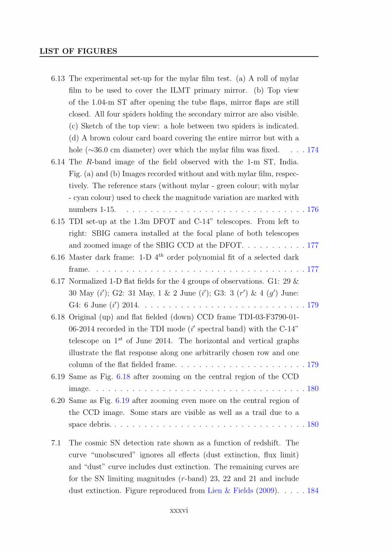
5.10 Air compressor (left panel) and air receiver (right panel) kept inside
the storage room. . . . . . . . . . . . . . . . . . . . . . . . . . . . . . 154
5.11 Air membrane dryer (left panel) and dew point sensor (right panel) . 154
6.1 Speed variation during the continuous rotation of the mirror (up to
90h). Image credit: AMOS . . . . . . . . . . . . . . . . . . . . . . . . 160
6.2 Speed variation test with 60 L of water. Peaks between ∼60s and
∼150s are seen because of water pouring disturbances. The system
started to stabilize after 360s. Image credit: AMOS. . . . . . . . . . . 160
6.3 Evolution of the PU temperature with time. . . . . . . . . . . . . . . 161
6.4 Equal surface sections drawn on the container before the spin casting. 163
6.5 Spin casting preparation. (a) Measured quantity of PU: Base resin,
part -A (white bucket) and hardener part -B (blue bucket). (b) PU
mixing process. . . . . . . . . . . . . . . . . . . . . . . . . . . . . . . 164
6.6 Pouring of the PU over the surface of the container. Each of the six
sectors were poured at the same time with the continuously rotating
container. . . . . . . . . . . . . . . . . . . . . . . . . . . . . . . . . . 165
6.7 Mercury vapor concentration as a function of time for the NASA
liquid mirror at NODO. Figure from Mulrooney PhD thesis. . . . . . 167
6.8 Peristaltic pump . . . . . . . . . . . . . . . . . . . . . . . . . . . . . 169
6.9 Setup to measure mercury vapors generated during the mercury tests. 170
6.10 Panel (a) Testing and cleaning the container with water. Panel (b)
Pouring mercury into the container. The shining mercury can be seen
in the central part of the dish. . . . . . . . . . . . . . . . . . . . . . . 171
6.11 Panel (a): Rotating mercury filled container by hand. Panel (b) Final
shape of the rotating mercury mirror. . . . . . . . . . . . . . . . . . 171
6.12 Experimental set-up for the surface quality test. . . . . . . . . . . . 173
xxxv
LIST OF FIGURES
6.13 The experimental set-up for the mylar film test. (a) A roll of mylar
film to be used to cover the ILMT primary mirror. (b) Top view
of the 1.04-m ST after opening the tube flaps, mirror flaps are still
closed. All four spiders holding the secondary mirror are also visible.
(c) Sketch of the top view: a hole between two spiders is indicated.
(d) A brown colour card board covering the entire mirror but with a
hole (∼36.0 cm diameter) over which the mylar film was fixed. . . . 174
6.14 The R-band image of the field observed with the 1-m ST, India.
Fig. (a) and (b) Images recorded without and with mylar film, respec-
tively. The reference stars (without mylar - green colour; with mylar
- cyan colour) used to check the magnitude variation are marked with
numbers 1-15. . . . . . . . . . . . . . . . . . . . . . . . . . . . . . . 176
6.15 TDI set-up at the 1.3m DFOT and C-14” telescopes. From left to
right: SBIG camera installed at the focal plane of both telescopes
and zoomed image of the SBIG CCD at the DFOT. . . . . . . . . . . 177
6.16 Master dark frame: 1-D 4th order polynomial fit of a selected dark
frame. . . . . . . . . . . . . . . . . . . . . . . . . . . . . . . . . . . . 177
6.17 Normalized 1-D flat fields for the 4 groups of observations. G1: 29 &
30 May (i′); G2: 31 May, 1 & 2 June (i′); G3: 3 (r′) & 4 (g′) June:
G4: 6 June (i′) 2014. . . . . . . . . . . . . . . . . . . . . . . . . . . . 179
6.18 Original (up) and flat fielded (down) CCD frame TDI-03-F3790-01-
06-2014 recorded in the TDI mode (i′ spectral band) with the C-14”
telescope on 1st of June 2014. The horizontal and vertical graphs
illustrate the flat response along one arbitrarily chosen row and one
column of the flat fielded frame. . . . . . . . . . . . . . . . . . . . . . 179
6.19 Same as Fig. 6.18 after zooming on the central region of the CCD
image. . . . . . . . . . . . . . . . . . . . . . . . . . . . . . . . . . . . 180
6.20 Same as Fig. 6.19 after zooming even more on the central region of
the CCD image. Some stars are visible as well as a trail due to a
space debris. . . . . . . . . . . . . . . . . . . . . . . . . . . . . . . . . 180
7.1 The cosmic SN detection rate shown as a function of redshift. The
curve “unobscured” ignores all effects (dust extinction, flux limit)
and “dust” curve includes dust extinction. The remaining curves are
for the SN limiting magnitudes (r-band) 23, 22 and 21 and include
dust extinction. Figure reproduced from Lien & Fields (2009). . . . . 184
xxxvi
LIST OF FIGURES
7.2 A plot showing the ILMT limiting magnitudes for the g′, r′ and i′
filters. The parameters to estimate these values are discussed in
Sect. 7.2. The X-axis represents the magnitude and the Y-axis rep-
resents the signal-to-noise ratio and the corresponding error in mag-
nitude. In this plot, the results for the three filters i.e. g′ (in red),
r′ (in blue) and i′ (in black) have been reproduced for the exposure
of a single scan (i.e. 102 sec) and three scans (i.e. 306 sec). Around
0.5 mag is gained once we stage images taken on three nights in any
single filter. . . . . . . . . . . . . . . . . . . . . . . . . . . . . . . . . 188
7.3 Evolution of the SN rate with the redshift (z) for CCSNe and Type
Ia. The continuous curves indicate the modelled SNe rate from Oguri
& Marshall (2010). Open squares are from recent CCSNe studies
of Bazin et al. (2009); Botticella et al. (2008); Dahlen et al. (2004)
and the filled squares represent Type Ia studies from Blanc et al.
(2004); Botticella et al. (2008); Dahlen et al. (2008, 2004); Dilday
et al. (2008); Hardin et al. (2000); Horesh et al. (2008); Kuznetsova
et al. (2008); Neill et al. (2006); Pain et al. (2002); Poznanski et al.
(2007b). Figure taken from Oguri & Marshall (2010). . . . . . . . . . 190
7.4 Illustration of the proposed processing data flow for SNe detection
and follow-up scheme. Upper left is a sketch of the ILMT and lower
left: images of the 3.6m and 1.3m optical telescopes and ILMT are
indicated. . . . . . . . . . . . . . . . . . . . . . . . . . . . . . . . . . 193
7.5 Image subtraction. Right panel: Galaxy UGC 01626 image with
SN 2011fu. The SN can be seen in one of the spiral arms indicated
by a circle. Left panel: Subtracted image where the SN is clearly
visible without galaxy contamination. . . . . . . . . . . . . . . . . . . 194
7.6 Demonstration of the spectra identification with the SNID code. The
flux is in arbitrary units. Observed and template spectra are shown
with black and red, respectively. The best fitted template is SN 1993J
(shown in the top left, blue characters with the estimated phase (+68)
relative to the light maximum). . . . . . . . . . . . . . . . . . . . . . 198
xxxvii
LIST OF FIGURES
7.7 Present and upcoming facilities at ARIES, Manora peak and Dev-
asthal observatories. Top left and right panels: 1.04m ST and 0.5m
Schmidt telescope, respectively. Bottom left and right panels are the
images of the 1.3m DFOT and upcoming 3.6m DOT telescopes, re-
spectively. These facilities will be used for the followup observations
of the ILMT detected SNe and other transient events for photometry
and/or spectroscopy. . . . . . . . . . . . . . . . . . . . . . . . . . . . 199
8.1 Lay-out of the ILMT location at Devasthal, India. The main en-
closure is on the right side of the image where the central pier is
indicated with a circle. The air compressor room is located left to
the main enclosure (central top in the image). Image credit: PPS. . . 207
8.2 Sketch of the front face of the proposed ILMT enclosure. The full
structure will be established over the concrete pillars. The top of the
roof is inclined in order to avoid as much as possible the effects of the
prevailing wind. Image credit: PPS. . . . . . . . . . . . . . . . . . . . 208
8.3 Present status of the ILMT enclosure along with the compressor room
(front). The enclosure of the upcoming 3.6m DOT telescope is also
visible in the background. . . . . . . . . . . . . . . . . . . . . . . . . 209
8.4 Computer clusters installed at the Poznan Observatory, Poland. These
machines will be later used for the ILMT data base as well as for the
image processing. . . . . . . . . . . . . . . . . . . . . . . . . . . . . . 211
xxxviii
List of Tables
1.1 Core-collapse SN fractions from theoretical models (rotating and non-
rotating) and observed samples (see text). . . . . . . . . . . . . . . . 25
2.1 Extinction, distance, and reddening values for the Carina region col-
lected from the literature. . . . . . . . . . . . . . . . . . . . . . . . . 48
2.2 Cross-identification of 43 X-ray sources from Claeskens et al. (2011)
with CrW optical photometry. Stars brighter than V = 11.3 are
from the literature. The YSOs identified in Section 2.4.2 are also
mentioned in the last column. . . . . . . . . . . . . . . . . . . . . . . 62
2.3 Sample of the optically identified YSO candidates along with their
derived ages and masses. Error bars in magnitude and colour rep-
resent formal internal (comparative) errors and do not include the
colour transformation and zero-point uncertainties. . . . . . . . . . . 65
2.4 The YSO cores identified in the CrW region and their characteristics. 75
3.1 Identification number (ID), coordinates (α, δ) and calibrated magni-
tudes of standard stars in the field of SN 2011fu. . . . . . . . . . . . . 86
3.2 Photometric observational log of SN 2011fu . . . . . . . . . . . . . . 89
3.3 Log of spectroscopic observations of SN 2011fu. . . . . . . . . . . . . 91
3.4 Epochs of the LC valley (tv) and the secondary peak (tp) in days after
explosion, and their respective apparent magnitudes for SN 2011fu
and SN 1993J. . . . . . . . . . . . . . . . . . . . . . . . . . . . . . . 91
3.5 Magnitude decay rate (in mag day−1) before valley (α1), rising rate
between valley to peak (α2) and decay rate after the peak (α3) for
SN 2011fu and SN 1993J. . . . . . . . . . . . . . . . . . . . . . . . . 94
3.6 Log of parameters derived from bolometric light curve modelling (Ku-
mar et al., 2013). . . . . . . . . . . . . . . . . . . . . . . . . . . . . . 100
xxxix
LIST OF TABLES
3.7 Velocities of the pseudo-photosphere, Hα and Hβ at different epochs
for SN 2011fu, derived with SYNOW. We assumed that the photospheric
velocity (Vphot) is equal to the velocity of Fe ii. All velocities are
given in km s−1. Tbb is the blackbody temperature of the pseudo-
photosphere in Kelvin degrees. The colour temperature (Tcol) de-
rived from the effective temperature − colour relations (see Bersten
& Hamuy, 2009; Dessart & Hillier, 2005b) is given in the last column. 105
4.1 Polarimetric observation log and estimated polarimetric parameters
of SN 2012aw. . . . . . . . . . . . . . . . . . . . . . . . . . . . . . . 115
4.2 Observational detail of 14 isolated field stars selected to subtract
the interstellar polarization. Observations of all field stars were per-
formed on 20 January 2013 in R band with the 1.04 m ST. All
these stars were selected with known distances and within 10 ra-
dius around SN 2012aw. The distance mentioned in the last column
has been taken from the van Leeuwen (2007) catalog. . . . . . . . . 117
4.3 Estimated polarimetric parameters for ISPMW (see Section 4.3.1 for
detail). . . . . . . . . . . . . . . . . . . . . . . . . . . . . . . . . . . 120
4.4 Observed and intrinsic (ISPMW and ISPMW + ISPHG subtracted) Q−U parameters for SN 2012aw. . . . . . . . . . . . . . . . . . . . . . . 127
5.1 Comparison between the characteristics of the LZT and ILMT. . . . . 140
5.2 Technical specifications of the 3.6m DOT and its instruments. . . . . 141
5.3 ILMT CCD chip (E2V-231) characteristics. . . . . . . . . . . . . . . . 148
5.4 Characteristics of the ILMT filters . . . . . . . . . . . . . . . . . . . . 150
5.5 Technical specifications: air compressor and air receiver. . . . . . . . 155
5.6 Technical specifications: Beko membrane dryer. . . . . . . . . . . . . 155
5.7 Technical specifications: Vaisala dew point and temperature trans-
mitter. . . . . . . . . . . . . . . . . . . . . . . . . . . . . . . . . . . 155
6.1 Zonal radial position . . . . . . . . . . . . . . . . . . . . . . . . . . . 162
6.2 Polyurethane Properties . . . . . . . . . . . . . . . . . . . . . . . . . 162
6.3 Some facts about mercury. . . . . . . . . . . . . . . . . . . . . . . . . 167
7.1 Different parameters used to calculate the ILMT limiting magnitude.
See also Finet (2013). . . . . . . . . . . . . . . . . . . . . . . . . . . 187
xl
LIST OF TABLES
7.2 Volume of the sky for different redshifts. . . . . . . . . . . . . . . . . 189
7.3 Predicted SNe Ia discovery rates for different redshifts. These num-
bers are estimated for a 4m diameter LMT similar to the ILMT. . . . 191
A.1 List of the optically identified YSOs along with their derived ages
and masses. . . . . . . . . . . . . . . . . . . . . . . . . . . . . . . . . 214
xli


Part I
Introduction
1

Chapter 1
Massive stars, supernovae and
liquid mirror telescopes
1.1 Massive stars
There are billions of stars in our universe with different physical properties (e.g.,
mass, size, temperature, and age). Stars with an initial mass greater than 8 M⊙
are broadly classified as massive stars. Rigel, Betelgeuse and Deneb having mass
between 15 to 19 M⊙ are a few examples of Galactic massive stars, prominently
visible with the naked eye. Although in the present-day universe, massive stars
are less in number than low and intermediate mass stars (see Kolmogorov, 1941;
Salpeter, 1955), their paramount role in astrophysics is well known. They are usually
born within the dense core of giant molecular clouds. During their short lifetime,
the radiation output from these stars ionizes the interstellar medium and perhaps
affects the subsequent formation of stars in their surrounding environments (Abbott,
1982; Leitherer et al., 1992).
Massive stars generally end their life as catastrophic explosions and enrich the
interstellar medium in galaxies with the products of the various nucleosynthesis
processes that have occurred during their lifetime (see Arnett, 1995, 1996; Fowler &
Hoyle, 1964; Hoyle & Fowler, 1960; Woosley & Weaver, 1995). These explosions may
be sources of compact objects (neutron stars, black holes) and many high energy
objects such as pulsars, magnetars that occur when compact objects remain bound
in a binary system (e.g., Remillard & McClintock, 2006). Therefore, indeed massive
stars are very important astrophysical sources to understand the evolution of the
universe.
3
1. MASSIVE STARS, SUPERNOVAE AND LIQUID MIRRORTELESCOPES
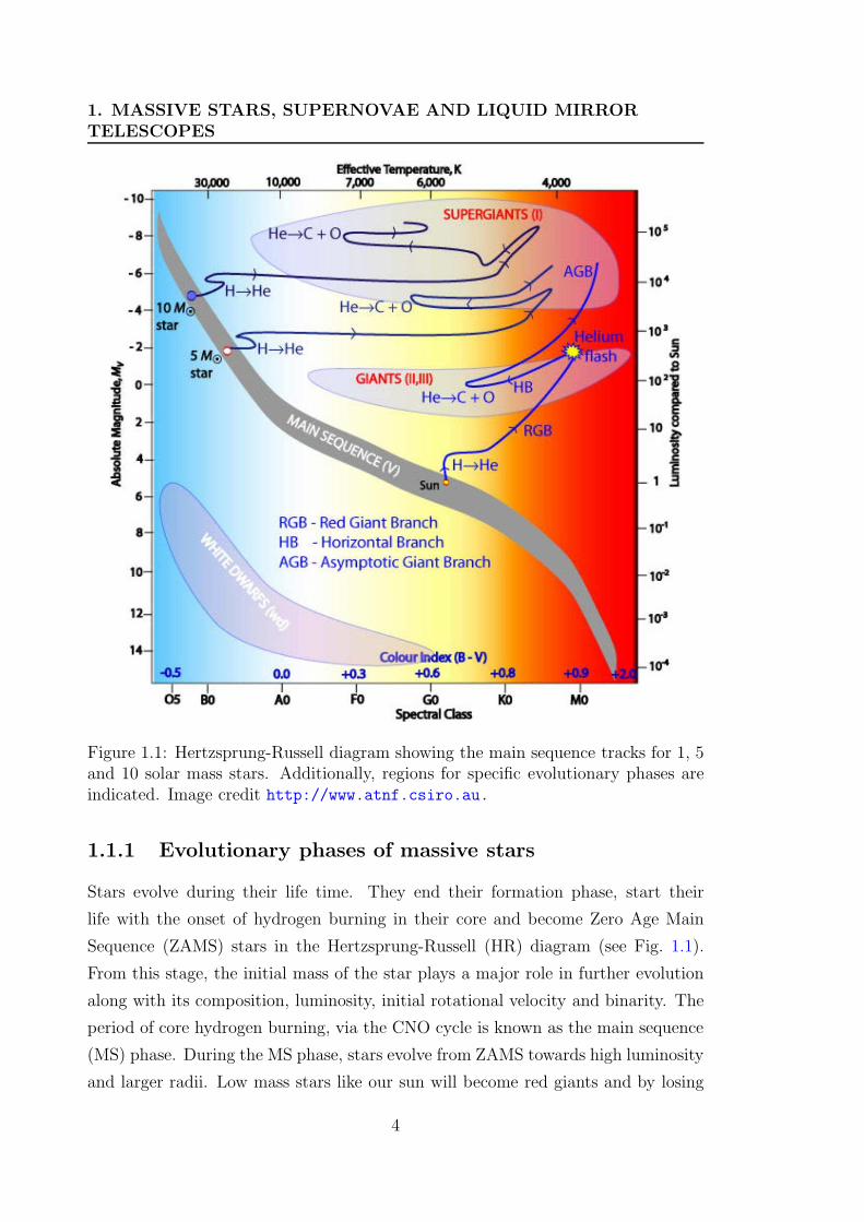
Figure 1.1: Hertzsprung-Russell diagram showing the main sequence tracks for 1, 5and 10 solar mass stars. Additionally, regions for specific evolutionary phases areindicated. Image credit http://www.atnf.csiro.au.
1.1.1 Evolutionary phases of massive stars
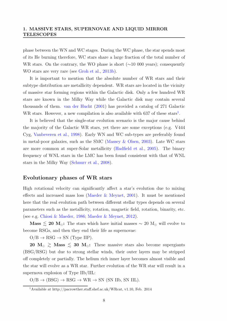
Stars evolve during their life time. They end their formation phase, start their
life with the onset of hydrogen burning in their core and become Zero Age Main
Sequence (ZAMS) stars in the Hertzsprung-Russell (HR) diagram (see Fig. 1.1).
From this stage, the initial mass of the star plays a major role in further evolution
along with its composition, luminosity, initial rotational velocity and binarity. The
period of core hydrogen burning, via the CNO cycle is known as the main sequence
(MS) phase. During the MS phase, stars evolve from ZAMS towards high luminosity
and larger radii. Low mass stars like our sun will become red giants and by losing
4
1.1 Massive stars
the outer shells of their atmosphere, they will finally cool to become white dwarfs.
Massive stars start at the ZAMS as an O or early B spectral type. On the main
sequence, they will gradually increase in radius, reducing their effective temperature
and to some extent increase their luminosity. In their path of evolution, massive
stars may follow various phases like supergiant, luminous blue variable and Wolf-
Rayet, and finally end their life as supernova explosions. In the following section we
briefly describe different characteristics of these stars.
1.1.1.1 Supergiants (SGs)
Supergiant stars are evolved phases of massive stars. They tend to be situated
towards the top of the HR diagram to the right of the main sequence (see Fig. 1.1).
These stars can be broadly classified into three major groups.
• Red supergiants (RSGs)
Red supergiant stars are massive stars with spectral type M (Chiosi & Maeder,
1986). They may have initial masses less than ∼30 M⊙ (at solar metallicity)
evolving beyond the main sequence and passing a fraction of their lives in the
cool upper region of the HR diagram. Mostly they have effective temperature
from 3000 K to 4000 K, and their luminosity is between 2 × 10⁴ - 6 × 10⁵
L⊙. These stars may lose mass at a rate of 10−6 to 10−4 M⊙ yr−1 (see Mauron
& Josselin, 2011). Their radii are very huge, typically 500–1500 R⊙. RSGs
are proposed as metallicity indicators (Bergemann et al., 2012, 2013; Davies
et al., 2010). They are also proposed as distance and age indicators (see
Lancon et al., 2009). Examples: Betelgeuse, Mu Cephei, VY Canis Majoris,
KW Sagitarii.
• Blue supergiants (BSGs)
Blue supergiants are very hot and bright stars. They are classified as spectral
class B or A (Chiosi & Maeder, 1986) and may have surface temperatures be-
tween 20,000K and 50,000K. These stars are highly illustrated in the night sky
because of their extreme luminosity. They typically appear in open clusters,
irregular galaxies, or the arms of spiral galaxies. At a solar metallicity, recent
modelling by Ekstrom et al. (2012) indicates that a star with a sufficiently
large initial mass ignites He in the center during the BSG stage, evolves to
the RSG region, and returns to the BSG region during He burning (blue-red-
blue evolution). The degree of mixing in radiative layers and the strength of
5
1. MASSIVE STARS, SUPERNOVAE AND LIQUID MIRRORTELESCOPES
wind mass loss govern the lowest initial mass for the blue-red-blue evolution.
Examples: Rigel, Sk-69 202, Sher 25.
• Yellow supergiants (YSGs)
These are rare stars which appear in the middle of the HR diagram (F to
G spectral type Chiosi & Maeder, 1986). Stars with initial masses between
approximately 9 M⊙ and 40 M⊙ briefly pass through this region. Possibly
these stars are post-RSGs, and usually have strong mass loss (Drout et al.,
2012). In both binary and single-star models, the lifetime of the YSG phase
is short-lived, only on the order of tens of thousands of years. Examples: Q
Cas, V509 Cas (HD 217476).
1.1.1.2 Luminous blue variables (LBVs)
Luminous blue variable stars (also known as S Doradus stars) were first defined by
Conti (1984). LBVs are very massive and intrinsically bright stars. They evolve
from O-type main sequence stars to become Wolf-Rayet stars. LBVs are highly
luminous (106 L⊙), exhibit high mass-loss (up to 10−4 M⊙ yr−1) and sometimes
giant eruptions occur (e.g. η Car). They are remarkably photometrically as well
as spectroscopically variable on timescales of years (short S Dor phases) to decades
(long S Dor phases, c.f. van Genderen, 2001). A significant increase in the degree
of mass loss rate also appears in the form of a variability. Most of LBVs have
strong winds and strong emission-line spectra (see Humphreys & Davidson, 1994,
for various characteristics of LBVs).
On the basis of their luminosity and positions on the H-R diagram, LBVs can be
categorized into three broad luminosity types (see Humphreys & Davidson, 1994;
Vink, 2012): (i) The most luminous star, η Carinae, occupies a class of its own. (ii)
A group containing stars which range from – 11 > Mbol > – 9.9. It includes most of
the well-known LBVs: R127, S Dor, P Cyg and AG Car. (iii) The lowest luminosity
LBVs are classified as R71 type (see Wolf et al., 1981).
1.1.1.3 WR stars
In 1867, Wolf-Rayet (WR) stars were first identified in the Cygnus constellation by
Charles-Joseph-Etienne Wolf and Georges-Antoine-Pons Rayet. WR stars originate
from O-type stars and have a typical mass range of 10-25 M⊙. These stars spend
a lifetime of a few 105 Myr i.e. 10% of the MS O phase (Crowther, 2007). Due to
6
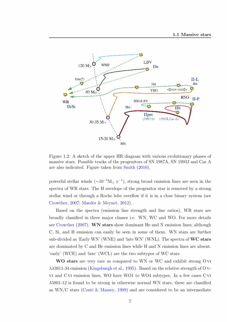
1.1 Massive stars
Figure 1.2: A sketch of the upper HR diagram with various evolutionary phases ofmassive stars. Possible tracks of the progenitors of SN 1987A, SN 1993J and Cas Aare also indicated. Figure taken from Smith (2010).
powerful stellar winds (∼10−5M⊙ y−1), strong broad emission lines are seen in the
spectra of WR stars. The H envelope of the progenitor star is removed by a strong
stellar wind or through a Roche lobe overflow if it is in a close binary system (see
Crowther, 2007; Maeder & Meynet, 2012).
Based on the spectra (emission line strength and line ratios), WR stars are
broadly classified in three major classes i.e. WN, WC and WO. For more details
see Crowther (2007). WN stars show dominant He and N emission lines; although
C, Si, and H emission can easily be seen in some of them. WN stars are further
sub-divided as ‘Early WN’ (WNE) and ‘late WN’ (WNL). The spectra ofWC stars
are dominated by C and He emission lines while H and N emission lines are absent.
‘early’ (WCE) and ‘late’ (WCL) are the two subtypes of WC stars.
WO stars are very rare as compared to WN or WC and exhibit strong Ovi
λλ3811-34 emission (Kingsburgh et al., 1995). Based on the relative strength of Ov-
vi and Cvi emission lines, WO have WO1 to WO4 subtypes. In a few cases Cvi
λ5801-12 is found to be strong in otherwise normal WN stars, these are classified
as WN/C stars (Conti & Massey, 1989) and are considered to be an intermediate
7
1. MASSIVE STARS, SUPERNOVAE AND LIQUID MIRRORTELESCOPES
phase between the WN and WC stages. During the WC phase, the star spends most
of its He burning therefore, WC stars share a large fraction of the total number of
WR stars. On the contrary, the WO phase is short (∼10 000 years); consequently
WO stars are very rare (see Groh et al., 2013b).
It is important to mention that the absolute number of WR stars and their
subtype distribution are metallicity dependent. WR stars are located in the vicinity
of massive star forming regions within the Galactic disk. Only a few hundred WR
stars are known in the Milky Way while the Galactic disk may contain several
thousands of them. van der Hucht (2001) has provided a catalog of 271 Galactic
WR stars. However, a new compilation is also available with 637 of these stars1.
It is believed that the single-star evolution scenario is the major cause behind
the majority of the Galactic WR stars, yet there are some exceptions (e.g. V444
Cyg, Vanbeveren et al., 1998). Early WN and WC sub-types are preferably found
in metal-poor galaxies, such as the SMC (Massey & Olsen, 2003). Late WC stars
are more common at super-Solar metallicity (Hadfield et al., 2005). The binary
frequency of WNL stars in the LMC has been found consistent with that of WNL
stars in the Milky Way (Schnurr et al., 2008).
Evolutionary phases of WR stars
High rotational velocity can significantly affect a star’s evolution due to mixing
effects and increased mass loss (Maeder & Meynet, 2001). It must be mentioned
here that the real evolution path between different stellar types depends on several
parameters such as the metallicity, rotation, magnetic field, rotation, binarity, etc.
(see e.g. Chiosi & Maeder, 1986; Maeder & Meynet, 2012).
Mass . 20 M⊙: The stars which have initial masses ∼ 20 M⊙ will evolve to
become RSGs, and then they end their life as supernovae:
O/B → RSG → SN (Type IIP).
20 M⊙ & Mass . 30 M⊙: These massive stars also become supergiants
(BSG/RSG) but due to strong stellar winds, their outer layers may be stripped
off completely or partially. The helium rich inner layer becomes almost visible and
the star will evolve as a WR star. Further evolution of the WR star will result in a
supernova explosion of Type IIb/IIL:
O/B → (BSG) → RSG → WR → SN (SN IIb, SN IIL).
1Available at http://pacrowther.staff.shef.ac.uk/WRcat, v1.10, Feb. 2014
8
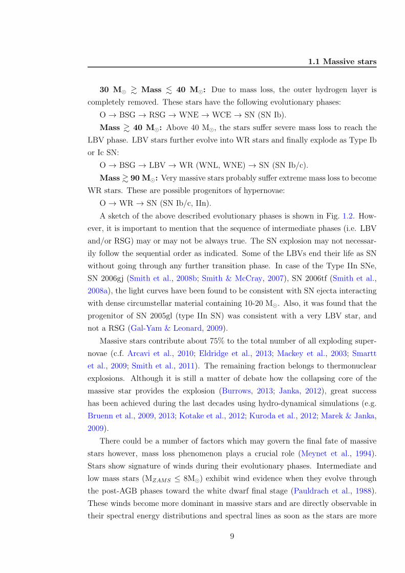
1.1 Massive stars
30 M⊙ & Mass . 40 M⊙: Due to mass loss, the outer hydrogen layer is
completely removed. These stars have the following evolutionary phases:
O → BSG → RSG → WNE → WCE → SN (SN Ib).
Mass & 40 M⊙: Above 40 M⊙, the stars suffer severe mass loss to reach the
LBV phase. LBV stars further evolve into WR stars and finally explode as Type Ib
or Ic SN:
O → BSG → LBV → WR (WNL, WNE) → SN (SN Ib/c).
Mass & 90 M⊙: Very massive stars probably suffer extreme mass loss to become
WR stars. These are possible progenitors of hypernovae:
O → WR → SN (SN Ib/c, IIn).
A sketch of the above described evolutionary phases is shown in Fig. 1.2. How-
ever, it is important to mention that the sequence of intermediate phases (i.e. LBV
and/or RSG) may or may not be always true. The SN explosion may not necessar-
ily follow the sequential order as indicated. Some of the LBVs end their life as SN
without going through any further transition phase. In case of the Type IIn SNe,
SN 2006gj (Smith et al., 2008b; Smith & McCray, 2007), SN 2006tf (Smith et al.,
2008a), the light curves have been found to be consistent with SN ejecta interacting
with dense circumstellar material containing 10-20 M⊙. Also, it was found that the
progenitor of SN 2005gl (type IIn SN) was consistent with a very LBV star, and
not a RSG (Gal-Yam & Leonard, 2009).
Massive stars contribute about 75% to the total number of all exploding super-
novae (c.f. Arcavi et al., 2010; Eldridge et al., 2013; Mackey et al., 2003; Smartt
et al., 2009; Smith et al., 2011). The remaining fraction belongs to thermonuclear
explosions. Although it is still a matter of debate how the collapsing core of the
massive star provides the explosion (Burrows, 2013; Janka, 2012), great success
has been achieved during the last decades using hydro-dynamical simulations (e.g.
Bruenn et al., 2009, 2013; Kotake et al., 2012; Kuroda et al., 2012; Marek & Janka,
2009).
There could be a number of factors which may govern the final fate of massive
stars however, mass loss phenomenon plays a crucial role (Meynet et al., 1994).
Stars show signature of winds during their evolutionary phases. Intermediate and
low mass stars (MZAMS ≤ 8M⊙) exhibit wind evidence when they evolve through
the post-AGB phases toward the white dwarf final stage (Pauldrach et al., 1988).
These winds become more dominant in massive stars and are directly observable in
their spectral energy distributions and spectral lines as soon as the stars are more
9
1. MASSIVE STARS, SUPERNOVAE AND LIQUID MIRRORTELESCOPES
luminous than 104 L⊙ in the HR diagram (for massive stars of spectral type O,
B, and A; Kudritzki & Puls, 2000). The strength of wind depends upon various
parameters such as luminosity (L), mass (M), and metallicity (Z) (see Vink, 2008).
In luminous stars, stellar winds are the main cause of mass loss as strong radi-
ation pressure pushes the mass outside (see Castor et al., 1975; Pauldrach et al.,
1986). Mass losses play an important role in the advanced evolutionary stages and
consequently influence all the outputs of stellar evolution and nucleosynthesis. Mass
loss rates of OB stars reach about 10−5 M⊙ yr−1 with wind velocities up to 3000
km s−1. Due to high mass loss these stars (red giants and supergiants) suffer from
high extinction.
1.1.2 Massive stars forming regions and their environments
Massive stars are usually born in dense clusters. The formation of these stars orig-
inates with collapsing dense cores inside larger clumps of giant molecular clouds
(Williams et al., 2000). It is believed that most stars in our Galaxy are to be born
in massive star forming regions and therefore, in the neighborhood of massive stars
(see Briceno et al., 2007, and references therein). Presence of high mass stars in star
forming regions may profoundly influence their environments compared to those in
the regions where only low/intermediate mass stars form (see, e.g., Preibisch et al.,
2011c). First, their strong ionizing radiation, powerful stellar winds, and finally, su-
pernova explosions can disperse the surrounding natal molecular clouds (e.g., Freyer
et al., 2003), and thus terminate the star formation process. Secondly, the ioniza-
tion fronts and expanding superbubbles can also compress nearby clouds and con-
sequently trigger the formation of new generations of stars (e.g., Elmegreen, 1998;
Gritschneder et al., 2010; Preibisch & Zinnecker, 2007) and new cluster formation
(Beuther et al., 2008).
The dense gravitationally bound OB star clusters or loose unbound OB associa-
tions1 are the final products of massive star formation (Briceno et al., 2007; Lada &
Lada, 2003). The enormous amount of UV radiation from the OB stars ionizes the
surrounding hydrogen, which is termed as Hii region (also known as diffuse nebula
or emission nebula). Some of the classical examples of OB star clusters are Orion
Nebula Cluster (Hillenbrand, 1997; Hillenbrand & Hartmann, 1998); NGC 3603
(Drissen et al., 1995; Moffat et al., 1994); R136 (Massey & Hunter, 1998; Parker
1These are loose, easily identifiable concentrations of bright, high-mass stars (see Blaauw, 1964;Humphreys, 1978)
10
1.2 Core collapse supernovae
& Garmany, 1993). Scorpius OB2, Orion OB1 (Blaauw, 1964, 1991) are a few ex-
amples of OB associations. Studies of these regions have provided very important
information. However, it should also be kept in mind that these nearby quiescent
regions of low-mass star formation may not be representative, because most stars
in our Galaxy form in a very different environment (see Preibisch, 2011).
Characterizing the nature of PMS stars in the vicinity of massive stars may play
an important role to understand the characteristics and physical conditions of their
evolution. Different stages of PMS are grouped into Classes 0-I-II-III that represent
infalling protostars, evolved protostars, classical T-Tauri stars (CTTS) and Weak
line T Tauri stars (WTTS), respectively (cf. Feigelson & Montmerle, 1999). Both
CTTS and WTTS exhibit emission lines (Balmer emission lines of hydrogen) and
absorption line of Li 6707 A in their spectra but the near infra red (NIR) excess
is limited in WTTS. Recent X-ray observations (eg. Chandra or XMM-Newton) of
star clusters boosted general consensus to understand the physical processes of PMS
stars.
The Carina nebula in Carina (NGC 3372) provides a unique target for studies
of massive star feedback which hosts 65 known O-type stars, 3 WR stars and the
well known luminous blue variable η Car (see also Smith & Brooks, 2008, for more
details). This region represents the early stages of the birth of an OB association,
and it is an environment where this young OB association is triggering the birth of
a second generation of stars as they destroy their own natal giant molecular cloud
(see Smith & Brooks, 2007). As most of the very massive stars in this complex are
located in several clusters (e.g. Tr14, 15 and 16 etc.), a number of wide field surveys
have been performed (for example, see Preibisch et al., 2011a,c,d; Roccatagliata
et al., 2013; Smith, 2006a; Smith et al., 2010, and references therein).
We have studied the stellar content in a wide field located west of η Carinae and
centered on the WN7ha + O binary system WR 22 (HD 92740). The data analysis
and results are presented in Chapter 2.
1.2 Core collapse supernovae
In general, lives of massive stars end after millions of years with a catastrophic
explosion. Some of these stellar explosions are termed supernovae (SN, plural: su-
pernovae, SNe). Core collapse supernovae (CCSNe) are end stages of those massive
stars which have a mass ≥ 8 M⊙. An enormous amount of energy (order of 1046
11
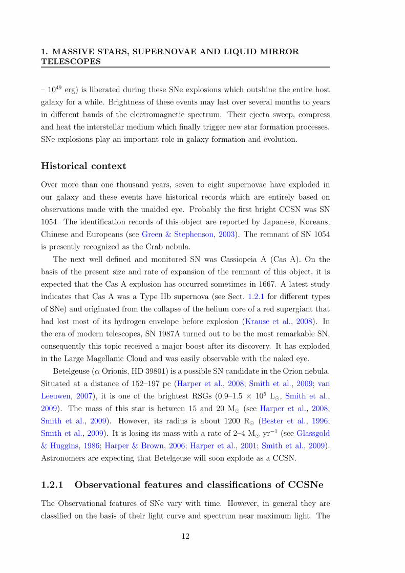
1. MASSIVE STARS, SUPERNOVAE AND LIQUID MIRRORTELESCOPES
– 1049 erg) is liberated during these SNe explosions which outshine the entire host
galaxy for a while. Brightness of these events may last over several months to years
in different bands of the electromagnetic spectrum. Their ejecta sweep, compress
and heat the interstellar medium which finally trigger new star formation processes.
SNe explosions play an important role in galaxy formation and evolution.
Historical context
Over more than one thousand years, seven to eight supernovae have exploded in
our galaxy and these events have historical records which are entirely based on
observations made with the unaided eye. Probably the first bright CCSN was SN
1054. The identification records of this object are reported by Japanese, Koreans,
Chinese and Europeans (see Green & Stephenson, 2003). The remnant of SN 1054
is presently recognized as the Crab nebula.
The next well defined and monitored SN was Cassiopeia A (Cas A). On the
basis of the present size and rate of expansion of the remnant of this object, it is
expected that the Cas A explosion has occurred sometimes in 1667. A latest study
indicates that Cas A was a Type IIb supernova (see Sect. 1.2.1 for different types
of SNe) and originated from the collapse of the helium core of a red supergiant that
had lost most of its hydrogen envelope before explosion (Krause et al., 2008). In
the era of modern telescopes, SN 1987A turned out to be the most remarkable SN,
consequently this topic received a major boost after its discovery. It has exploded
in the Large Magellanic Cloud and was easily observable with the naked eye.
Betelgeuse (α Orionis, HD 39801) is a possible SN candidate in the Orion nebula.
Situated at a distance of 152–197 pc (Harper et al., 2008; Smith et al., 2009; van
Leeuwen, 2007), it is one of the brightest RSGs (0.9–1.5 × 10⁵ L⊙, Smith et al.,
2009). The mass of this star is between 15 and 20 M⊙ (see Harper et al., 2008;
Smith et al., 2009). However, its radius is about 1200 R⊙ (Bester et al., 1996;
Smith et al., 2009). It is losing its mass with a rate of 2–4 M⊙ yr−1 (see Glassgold
& Huggins, 1986; Harper & Brown, 2006; Harper et al., 2001; Smith et al., 2009).
Astronomers are expecting that Betelgeuse will soon explode as a CCSN.
1.2.1 Observational features and classifications of CCSNe
The Observational features of SNe vary with time. However, in general they are
classified on the basis of their light curve and spectrum near maximum light. The
12
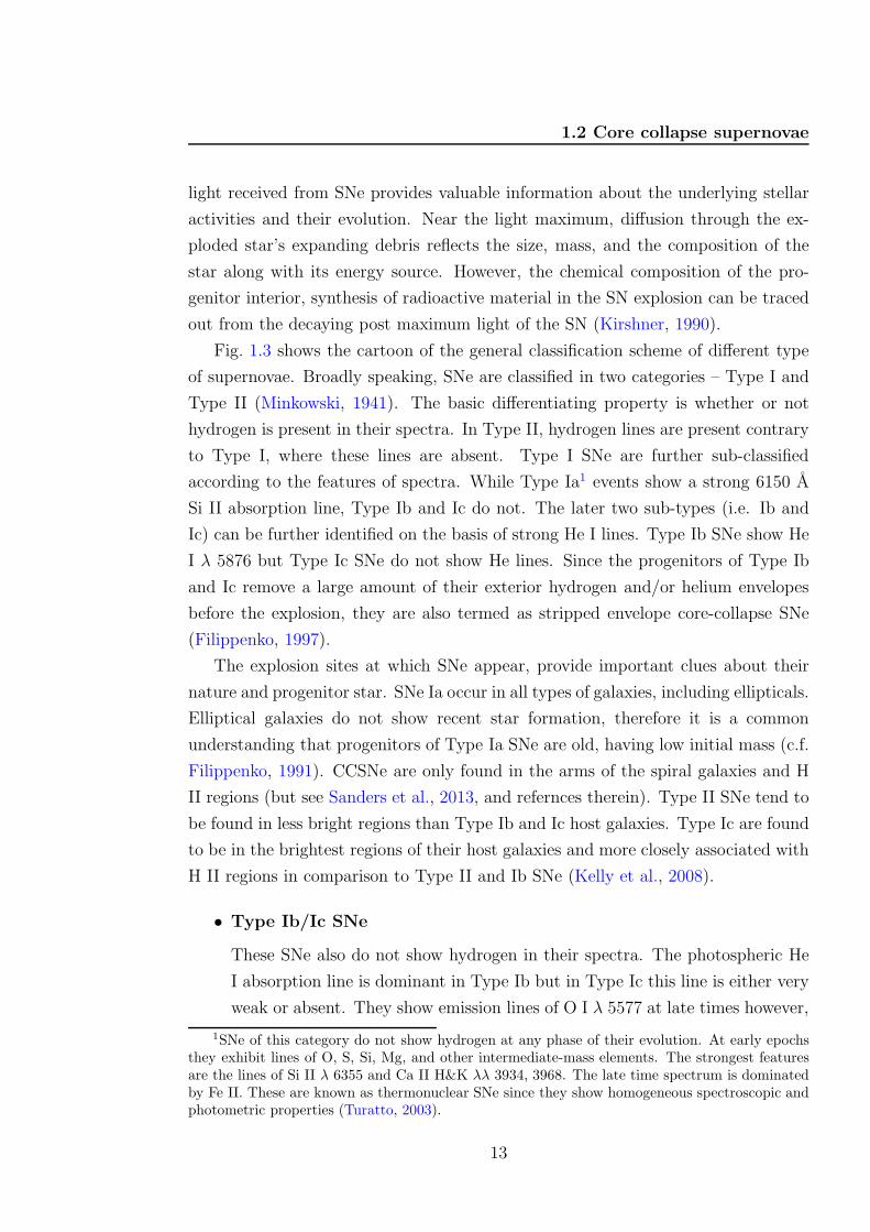
1.2 Core collapse supernovae
light received from SNe provides valuable information about the underlying stellar
activities and their evolution. Near the light maximum, diffusion through the ex-
ploded star’s expanding debris reflects the size, mass, and the composition of the
star along with its energy source. However, the chemical composition of the pro-
genitor interior, synthesis of radioactive material in the SN explosion can be traced
out from the decaying post maximum light of the SN (Kirshner, 1990).
Fig. 1.3 shows the cartoon of the general classification scheme of different type
of supernovae. Broadly speaking, SNe are classified in two categories – Type I and
Type II (Minkowski, 1941). The basic differentiating property is whether or not
hydrogen is present in their spectra. In Type II, hydrogen lines are present contrary
to Type I, where these lines are absent. Type I SNe are further sub-classified
according to the features of spectra. While Type Ia1 events show a strong 6150 A
Si II absorption line, Type Ib and Ic do not. The later two sub-types (i.e. Ib and
Ic) can be further identified on the basis of strong He I lines. Type Ib SNe show He
I λ 5876 but Type Ic SNe do not show He lines. Since the progenitors of Type Ib
and Ic remove a large amount of their exterior hydrogen and/or helium envelopes
before the explosion, they are also termed as stripped envelope core-collapse SNe
(Filippenko, 1997).
The explosion sites at which SNe appear, provide important clues about their
nature and progenitor star. SNe Ia occur in all types of galaxies, including ellipticals.
Elliptical galaxies do not show recent star formation, therefore it is a common
understanding that progenitors of Type Ia SNe are old, having low initial mass (c.f.
Filippenko, 1991). CCSNe are only found in the arms of the spiral galaxies and H
II regions (but see Sanders et al., 2013, and refernces therein). Type II SNe tend to
be found in less bright regions than Type Ib and Ic host galaxies. Type Ic are found
to be in the brightest regions of their host galaxies and more closely associated with
H II regions in comparison to Type II and Ib SNe (Kelly et al., 2008).
• Type Ib/Ic SNe
These SNe also do not show hydrogen in their spectra. The photospheric He
I absorption line is dominant in Type Ib but in Type Ic this line is either very
weak or absent. They show emission lines of O I λ 5577 at late times however,
1SNe of this category do not show hydrogen at any phase of their evolution. At early epochsthey exhibit lines of O, S, Si, Mg, and other intermediate-mass elements. The strongest featuresare the lines of Si II λ 6355 and Ca II H&K λλ 3934, 3968. The late time spectrum is dominatedby Fe II. These are known as thermonuclear SNe since they show homogeneous spectroscopic andphotometric properties (Turatto, 2003).
13
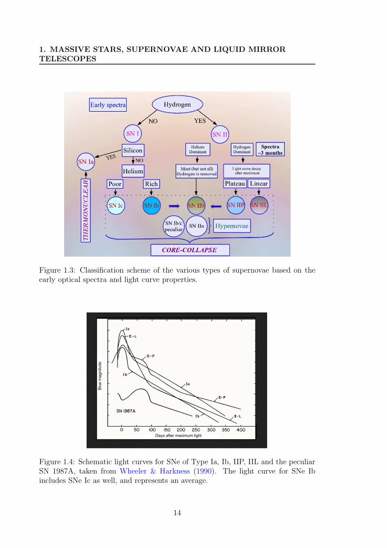
1. MASSIVE STARS, SUPERNOVAE AND LIQUID MIRRORTELESCOPES
Figure 1.3: Classification scheme of the various types of supernovae based on theearly optical spectra and light curve properties.
Figure 1.4: Schematic light curves for SNe of Type Ia, Ib, IIP, IIL and the peculiarSN 1987A, taken from Wheeler & Harkness (1990). The light curve for SNe Ibincludes SNe Ic as well, and represents an average.
14
1.2 Core collapse supernovae
maximum 3 weeks one year
Ηβ
Ηα
HeI
CaII SII
SiII
[Fe III]
[Fe II]+[Fe III]
[Co III]
Na I
[Ca II]
[O I]
[O I]
II
Ib
Ic
Ia
Ηα
Na I
Ca II
Ηα
O I
Figure 1.5: Spectral evolution of different types of SNe at various epochs – nearmaxima, 3 weeks and one year after maxima (from, Turatto, 2003)
Type Ic SNe exhibit strong features of O I λ 7774 absorption and Ca II H&K
absorption. The shape of the light curves (in B and V bands) of both SNe are
generally like those of Type Ia SNe but are less luminous by a factor of ∼4
than Type Ia (c.f. Filippenko, 1991).
There is a subclass of type Ib/Ic SNe which are known as “hypernovae”
(Woosley & Weaver, 1982). It is believed that hypernovae represent more
energetic events than normal CCSNe (kinetic energy > 1052 erg). A few exam-
ples of hypernovae are SN 1998bw (Iwamoto et al., 1998), SN 2002ap (Mazzali
et al., 2002), SN 2003dh (Mazzali et al., 2003), SN 1997ef (Mazzali et al.,
2000). Some of the Type Ic hypernovae have been found to be associated with
gamma ray bursts 1.
• Type IIP(‘Plateau’) SNe
These are the most common events in Type II. They contribute about 70%
of the total population of Type II SNe (Lennarz et al., 2012). The lumi-
1These are the most luminous explosions in the universe with intense flashes of gamma rays(10 keV - 10GeV) and lasting from a fraction of a second to up to a few minutes. They may releasean isotropic energy of the order of 1054 erg.
15
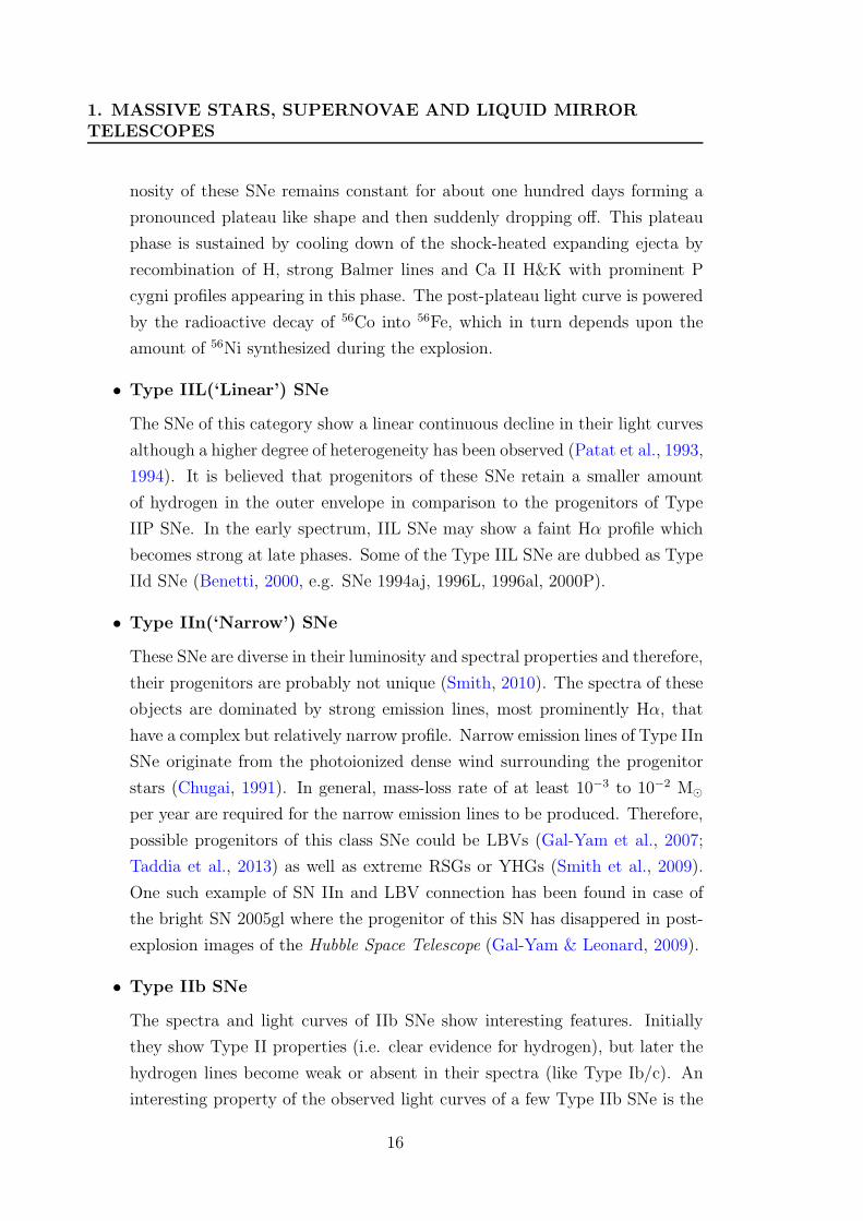
1. MASSIVE STARS, SUPERNOVAE AND LIQUID MIRRORTELESCOPES
nosity of these SNe remains constant for about one hundred days forming a
pronounced plateau like shape and then suddenly dropping off. This plateau
phase is sustained by cooling down of the shock-heated expanding ejecta by
recombination of H, strong Balmer lines and Ca II H&K with prominent P
cygni profiles appearing in this phase. The post-plateau light curve is powered
by the radioactive decay of 56Co into 56Fe, which in turn depends upon the
amount of 56Ni synthesized during the explosion.
• Type IIL(‘Linear’) SNe
The SNe of this category show a linear continuous decline in their light curves
although a higher degree of heterogeneity has been observed (Patat et al., 1993,
1994). It is believed that progenitors of these SNe retain a smaller amount
of hydrogen in the outer envelope in comparison to the progenitors of Type
IIP SNe. In the early spectrum, IIL SNe may show a faint Hα profile which
becomes strong at late phases. Some of the Type IIL SNe are dubbed as Type
IId SNe (Benetti, 2000, e.g. SNe 1994aj, 1996L, 1996al, 2000P).
• Type IIn(‘Narrow’) SNe
These SNe are diverse in their luminosity and spectral properties and therefore,
their progenitors are probably not unique (Smith, 2010). The spectra of these
objects are dominated by strong emission lines, most prominently Hα, that
have a complex but relatively narrow profile. Narrow emission lines of Type IIn
SNe originate from the photoionized dense wind surrounding the progenitor
stars (Chugai, 1991). In general, mass-loss rate of at least 10−3 to 10−2 M⊙
per year are required for the narrow emission lines to be produced. Therefore,
possible progenitors of this class SNe could be LBVs (Gal-Yam et al., 2007;
Taddia et al., 2013) as well as extreme RSGs or YHGs (Smith et al., 2009).
One such example of SN IIn and LBV connection has been found in case of
the bright SN 2005gl where the progenitor of this SN has disappered in post-
explosion images of the Hubble Space Telescope (Gal-Yam & Leonard, 2009).
• Type IIb SNe
The spectra and light curves of IIb SNe show interesting features. Initially
they show Type II properties (i.e. clear evidence for hydrogen), but later the
hydrogen lines become weak or absent in their spectra (like Type Ib/c). An
interesting property of the observed light curves of a few Type IIb SNe is the
16
1.2 Core collapse supernovae
initial peak and rapid decline, followed by a subsequent rise and a secondary
maximum (for example SN 1993J (Barbon et al., 1995; Richmond et al., 1994);
SN 2011dh (Arcavi et al., 2011) and SN 2011fu (Kumar et al., 2013)). The first
maximum is associated with the shock heating of the hydrogen-rich envelope
and the second maximum is caused by the radioactive decay of nickel (Benson
et al., 1994). Type IIb SNe are further divided into two subgroups: Type cIIb
with compact progenitors, (e.g. SNe 1996cb, 2001ig and 2008ax) and Type
eIIb with extended progenitors, such as SNe 1993J and 2001gd (Chevalier
& Soderberg, 2010). However, Maeda (2013) has expressed doubt about the
existence of these two subgroups.
• Superluminous SNe
In addition to the above described SNe, the past decade has seen the discov-
ery of plentiful superluminous supernovae (SLSNe). They are characterized
by peak magnitudes (MV . –21 mag) that are 2–3 magnitudes higher than
those of typical CCSNe and comparable, or brighter than Type Ia observed in
the nearby universe (Quimby et al., 2013). Till now around 20 SLSNe have
been discussed in the literature (see Gal-Yam, 2012). It should be noted that
although in comparison to other Types of SNe, the SNLSe number is very
small but due to their copious ultraviolet flux, these SLSN events may be-
come useful cosmic beacons enabling studies of distant star-forming galaxies
and their gaseous environments (Gal-Yam, 2012). Spectroscopically SLSNe
belong to Type IIn or Ic.
One of the possible mechanisms behind SLSNe is pair-instability. Extremely
massive stars in the mass range of 100 – 260 M⊙ may die in a thermonu-
clear runaway triggered by pair production instability and resulting as ther-
monuclear explosion known as pair instability supernova (PISN) (see Barkat
et al., 1967; Bisnovatyi-Kogan & Kazhdan, 1967; Fowler & Hoyle, 1964; Fra-
ley, 1967; Heger & Woosley, 2002; Kasen et al., 2011; Kippenhahn & Weigert,
1990; Rakavy & Shaviv, 1967). A number of SNe belonging to this class have
been discovered during the last few years (see Gal-Yam, 2012; Gal-Yam et al.,
2009; Quimby et al., 2011). PISN explosions completely disrupt very massive
stars and a huge amount of newly formed heavy elements are expelled in the
surrounding medium. Theoretical models predict that a PISN can produce
up to 55 M⊙ Ni (Heger & Woosley, 2002; Kozyreva et al., 2014; Umeda &
17
1. MASSIVE STARS, SUPERNOVAE AND LIQUID MIRRORTELESCOPES
Nomoto, 2002). However, in the case of SN 2007bi the spectral and photo-
metric analyses indicate that more than 3 M⊙ of Ni were ejected during the
explosion (Gal-Yam et al., 2009). This Ni mass production is significantly
higher than the normal CCSN explosion which is limited to about 0.5 M⊙
(Heger & Woosley, 2010; Umeda & Nomoto, 2008; Woosley & Weaver, 1995).
SLSNe could also arise due to the pulsational pair instability process (Woosley
et al., 2007) or magnetar-driven mechanisms (Dessart et al., 2012; Kasen &
Bildsten, 2010; Woosley, 2010).
1.2.2 Explosion mechanisms of CCSNe
The core collapse SNe arise due to the gravitational collapse of massive stars (M ≥ 8
M⊙). Various stages occuring in CCSNe are shown schematically in Fig. 1.6. At the
end stage of their evolutionary path massive stars reach the red supergiant phase
or blue supergiant phase and finally explode as supernovae. Several research groups
have performed detailed simulations for the pre-collapse evolutionary stages (see e.g.
Woosley et al., 2002; Woosley & Weaver, 1995). A series of nuclear reactions occur
before the explosion.
Starting from the fusion of hydrogen, the buildup of heavier elements in the core
of a massive star continues until the isotope of iron 56Fe is formed. The hydrogen
nuclei first fuse to form helium for a few million years in the core of the star until the
entire hydrogen is used up. Helium burning sets in when the core contracts, causing
an increase in the density and temperature and the Helium fusion forms carbon.
Simultaneously the hydrogen burning begins in the surrounding layers. After he-
lium is exhausted, the core contracts further and becomes dense and hot enough to
start the carbon burning to form oxygen and neon. Neon further undergoes photo-
rearrangement reactions with oxygen and magnesium. Oxygen burns to silicon and
silicon burning finally gives iron group elements through a series of reactions.
Since iron is the most stable nucleus, no further fusion reactions take place and
thus, finally the star has an inert Fe core surrounded by an onion shell structure
(left most in Fig. 1.6) in which silicon, oxygen, neon, carbon, helium, hydrogen are
burning in different layers. Electron degeneracy pressure holds the inert Fe core
against collapse under its own gravity. Ashes from the sorrounding burning layers
keep increasing the mass of the core. Once the core goes beyond the Chandrasekhar
limit of about 1.4M⊙ there is nothing to support it, and it collapses.
18
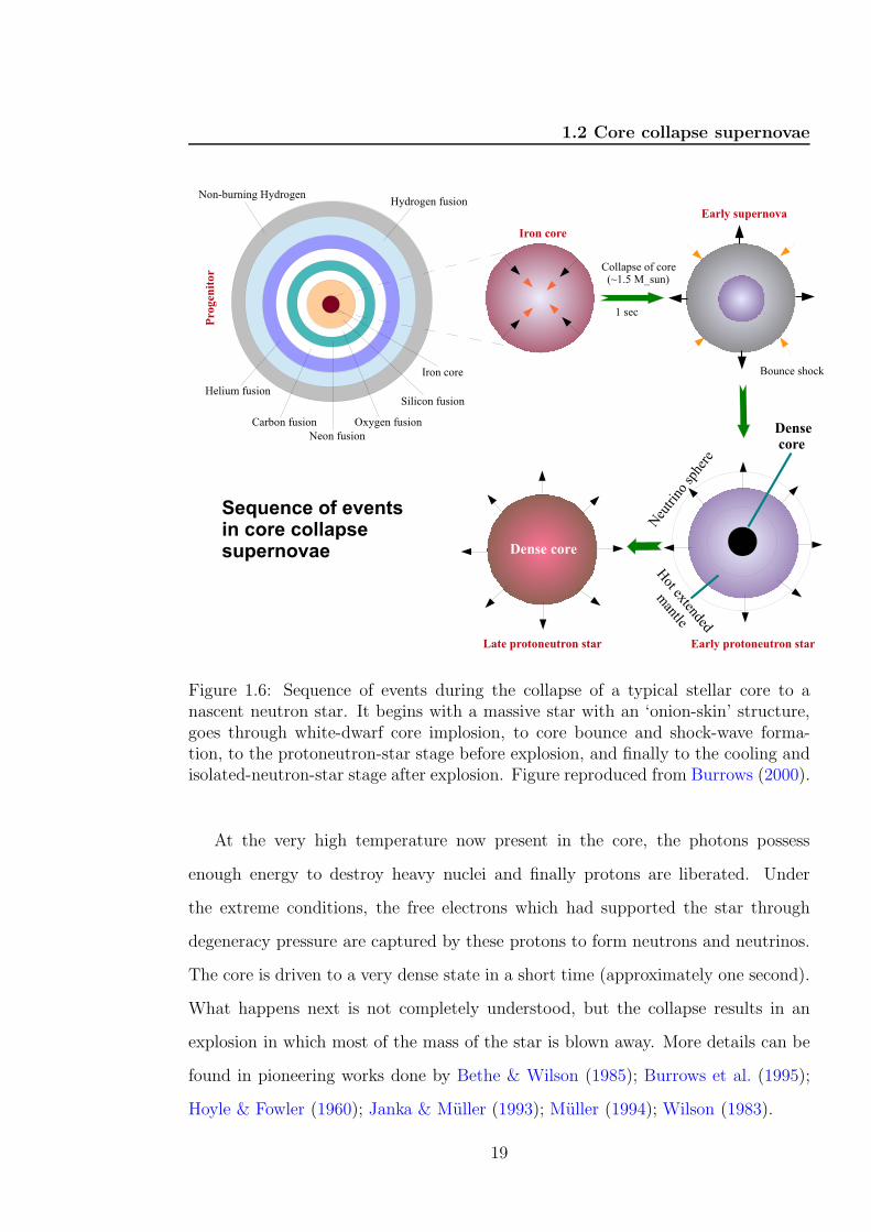
1.2 Core collapse supernovae
Figure 1.6: Sequence of events during the collapse of a typical stellar core to anascent neutron star. It begins with a massive star with an ‘onion-skin’ structure,goes through white-dwarf core implosion, to core bounce and shock-wave forma-tion, to the protoneutron-star stage before explosion, and finally to the cooling andisolated-neutron-star stage after explosion. Figure reproduced from Burrows (2000).
At the very high temperature now present in the core, the photons possess
enough energy to destroy heavy nuclei and finally protons are liberated. Under
the extreme conditions, the free electrons which had supported the star through
degeneracy pressure are captured by these protons to form neutrons and neutrinos.
The core is driven to a very dense state in a short time (approximately one second).
What happens next is not completely understood, but the collapse results in an
explosion in which most of the mass of the star is blown away. More details can be
found in pioneering works done by Bethe & Wilson (1985); Burrows et al. (1995);
Hoyle & Fowler (1960); Janka & Muller (1993); Muller (1994); Wilson (1983).
19
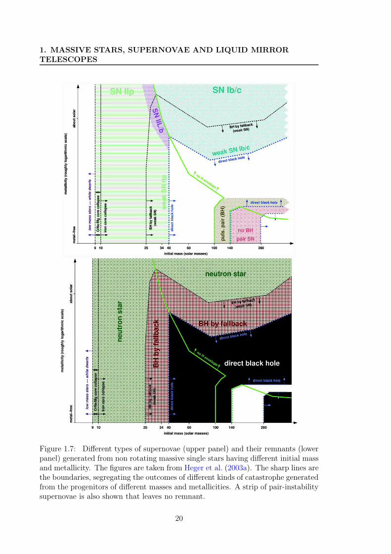
1. MASSIVE STARS, SUPERNOVAE AND LIQUID MIRRORTELESCOPES
Figure 1.7: Different types of supernovae (upper panel) and their remnants (lowerpanel) generated from non rotating massive single stars having different initial massand metallicity. The figures are taken from Heger et al. (2003a). The sharp lines arethe boundaries, segregating the outcomes of different kinds of catastrophe generatedfrom the progenitors of different masses and metallicities. A strip of pair-instabilitysupernovae is also shown that leaves no remnant.
20
1.2 Core collapse supernovae
Fate of the progenitors of CCSNe
The fate of the progenitors of CCSNe (i.e. massive stars) mainly depends upon their
mass, composition at birth and by the history of their mass loss. SN properties
depend on the progenitor mass in a complex way. Large differences in the explosion
characteristics are possible for small mass differences (Janka, 2012). In the literature,
it is often argued that massive stars with initial masses higher than about > 25–30
M⊙ collapse to form a black hole rather than a neutron star (Burrows, 2013; Fryer,
1999; Heger et al., 2003b). However, it is not fully understood which stars die as
bright supernovae leaving neutron stars as remnants and which stars collapse into
black holes with or without supernovae. For example recently Ugliano et al. (2012)
have investigated the question of the mass-dependence of the neutron star/black-
hole formation and show that stars less massive than 20 M⊙ can result in black holes
and stars of 20–40 M⊙ can end their evolution with the formation of a neutron star.
Fig. 1.7 represents the nature of the explosion (upper panel) and its remnant
(lower panel) on the basis of the initial mass of the progenitor and metallicity of the
environment. Here, the progenitor is assumed to be non-rotating. For each area (top
panel), the type of the SN is indicated. The shading on the bottom panel indicates
the area where formation of a black hole is expected; elsewhere, the remnant is a
neutron star. In between the dark shaded region (bottom panel, white colour), a
strip of pair-instability supernovae is also indicated which leave no remnant. See
Heger et al. (2003b) for more details.
1.2.3 Polarization properties of CCSNe
It is interesting that SNe are traditionally assumed to be spherically symmetric.
However, there are observational evidences such as aspherical structure of many
young Galactic SN remnants (see Fesen, 2001; Manchester, 1987), the asymmetric
distribution of material inferred from direct speckle imaging of young SNe (e.g.,
SN 1987A, Papaliolios et al., 1989) which indicate that there is an asymmetry in
the explosion mechanism and/or distribution of the SN ejecta (see also Filippenko
& Leonard, 2004).
The first SN polarization observations have been reported by Serkowski (1970).
But a direct observational test for the presence of asphericity in SNe was pro-
posed by Shapiro & Sutherland (1982). With growing attention in the SNe study,
subsequent polarimetric observations of additional SNe led to the conclusion that
21
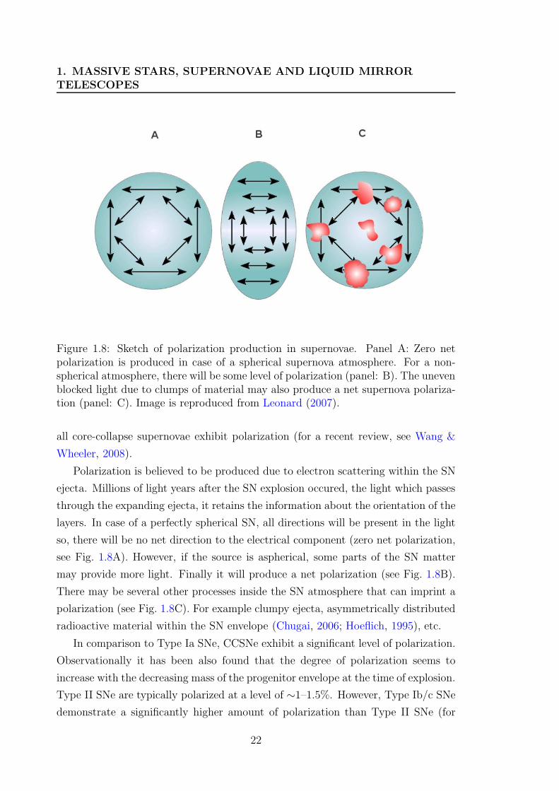
1. MASSIVE STARS, SUPERNOVAE AND LIQUID MIRRORTELESCOPES
Figure 1.8: Sketch of polarization production in supernovae. Panel A: Zero netpolarization is produced in case of a spherical supernova atmosphere. For a non-spherical atmosphere, there will be some level of polarization (panel: B). The unevenblocked light due to clumps of material may also produce a net supernova polariza-tion (panel: C). Image is reproduced from Leonard (2007).
all core-collapse supernovae exhibit polarization (for a recent review, see Wang &
Wheeler, 2008).
Polarization is believed to be produced due to electron scattering within the SN
ejecta. Millions of light years after the SN explosion occured, the light which passes
through the expanding ejecta, it retains the information about the orientation of the
layers. In case of a perfectly spherical SN, all directions will be present in the light
so, there will be no net direction to the electrical component (zero net polarization,
see Fig. 1.8A). However, if the source is aspherical, some parts of the SN matter
may provide more light. Finally it will produce a net polarization (see Fig. 1.8B).
There may be several other processes inside the SN atmosphere that can imprint a
polarization (see Fig. 1.8C). For example clumpy ejecta, asymmetrically distributed
radioactive material within the SN envelope (Chugai, 2006; Hoeflich, 1995), etc.
In comparison to Type Ia SNe, CCSNe exhibit a significant level of polarization.
Observationally it has been also found that the degree of polarization seems to
increase with the decreasing mass of the progenitor envelope at the time of explosion.
Type II SNe are typically polarized at a level of ∼1–1.5%. However, Type Ib/c SNe
demonstrate a significantly higher amount of polarization than Type II SNe (for
22
1.2 Core collapse supernovae
more details, see Gorosabel et al., 2006; Kawabata et al., 2003, 2002; Leonard &
Filippenko, 2001; Maund et al., 2013, 2007; Patat et al., 2012; Tanaka et al., 2012;
Wang et al., 2003a, and references therein).
We have studied the polarimetric properties of the Type II plateau supernova
SN 2012aw. The analysis and results are presented in Chapter 4.
1.2.4 Supernova rate: observational and theoretical overview
With a growing interest in supernovae science, several scientific groups such as the
Catalina Real-Time Transient Surveys (Drake et al., 2009), the Lick Observatory
Supernova Search (Leaman et al., 2009), the Palomar Transient Factory (Rau et al.,
2009), and the La Silla Quest (Hadjiyska et al., 2011) are engaged in supernovae dis-
covery. While the majority of SNe discoveries are done by professional astronomers,
groups of amateur astronomers also contribute significantly to it. There are also
many robotic telescopes which are involved in prompt optical observations of GRBs
and discovery of new SNe (e.g. the Robotic Optical Transient Search Experiment,
ROTSE (Akerlof et al., 2000), the Rapid Eye Mount, REM (Covino et al., 2004;
Cutispoto et al., 2004; Zerbi et al., 2004), the Globle Master Robotic Net). In ad-
dition, there are two upcoming big facilities like the Panoramic Survey Telescope
And Rapid Response System, Pan-STARRS (Hodapp et al., 2004) and the Large
Synoptic Survey Telescope, LSST (Ivezic et al., 2008). Both of these have a wide
field imaging facility which will be useful for transient imaging.
Along with the above cited ground based observatories, there are several space
based telescopes which are mainly used in high energy bands. Some of them are the
Swift (Barthelmy et al., 2005), the GALaxy Evolution eXplorer, GALEX (Martin
et al., 2005), the Rossi X-ray Timing explorer, RXT (Jahoda et al., 1996), the
Monitor of All-sky X-ray Image, MAXI (Matsuoka et al., 2009) and the Fermi
Large Area Telescope, LAT (Atwood et al., 2009). The most recently launched
GAIA spacecraft will possibly detect thousands of supernovae before they reach
their maximum brightness.
As can be seen from Fig. 1.9, the SNe discovery enhanced after the SN 1987A
event. Presently several hundreds of SNe are discovered every year, though the
number of bright SNe (brighter than 15 mag) is still very small. There have been a
few volume-limited studies of nearby CCSNe in different SNe search programs1 (e.g.
the Lick observatory Supernova Search, LOSS; the Katzman Automatic Imaging
1see also (Arcavi et al., 2010; Cappellaro et al., 1997; Li et al., 2011; Smartt et al., 2009)
23
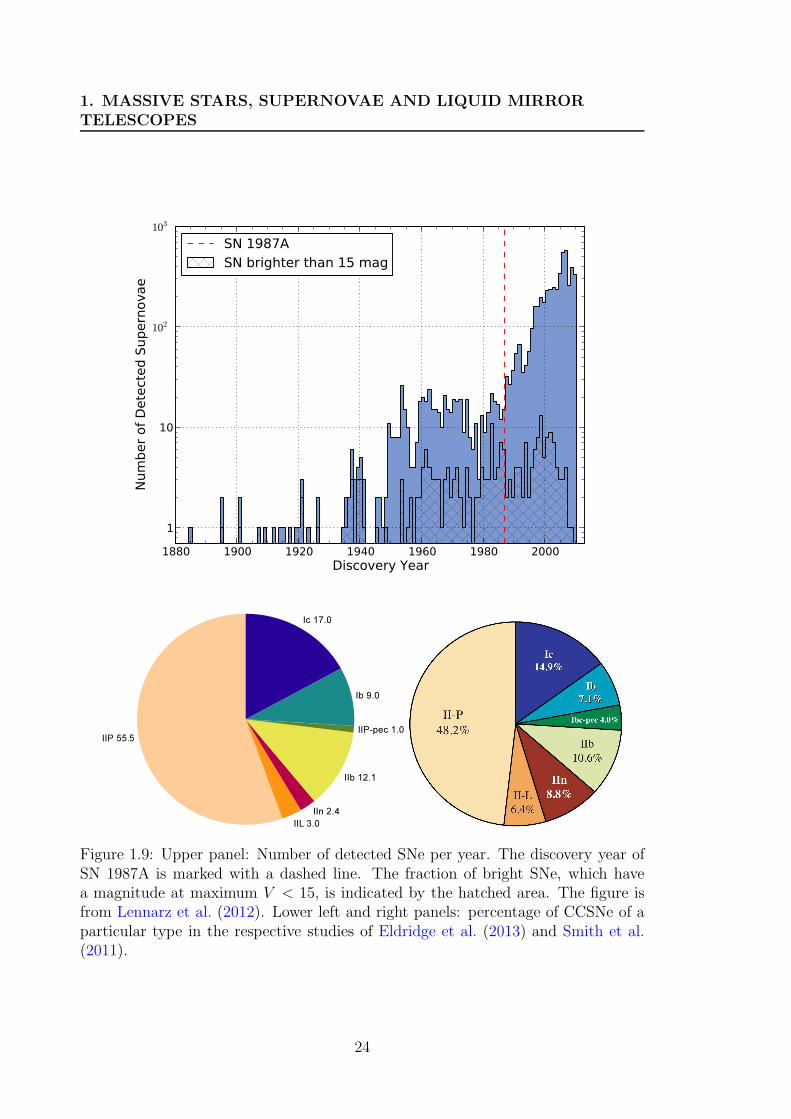
1. MASSIVE STARS, SUPERNOVAE AND LIQUID MIRRORTELESCOPES
Figure 1.9: Upper panel: Number of detected SNe per year. The discovery year ofSN 1987A is marked with a dashed line. The fraction of bright SNe, which havea magnitude at maximum V < 15, is indicated by the hatched area. The figure isfrom Lennarz et al. (2012). Lower left and right panels: percentage of CCSNe of aparticular type in the respective studies of Eldridge et al. (2013) and Smith et al.(2011).
24
1.3 Liquid mirror telescopes (LMTs)
Table 1.1: Core-collapse SN fractions from theoretical models (rotating and non-rotating) and observed samples (see text).
SN Non-rotating Rotating Observed sample (%) Observed sample (%)Type model (%) model (%) (Eldridge et al., 2013) (Smith et al., 2011)
IIP 70.7 64.9 55.5 ± 6.6 48.2 +5.7−5.6
IIL + IIb 16.2 13.1 15.1 ± 3.4 17.0 +4.6−4.0
IIn − − 2.4 ± 1.4 8.8 +3.3−2.9
IIpec − − 1.0 ± 0.9 −Ib 8.1 7.8 9.0 ± 2.7 8.4 +3.1
−2.6
Ic 5.0 14.2 17.0 ± 3.7 17.6 +4.2−3.8
Telescope, KAIT; the Palomar Transient Factory, PTF). Two most recent studies
of the observed fraction of CCSNe have been analysed by Smith et al. (2011) and
Eldridge et al. (2013). Their results are presented in the lower left and right panels
of Fig. 1.9 and summarized in Table 1.1. It is obvious from this figure that the
majority of CCSNe belong to the Type II category.
Recently, Groh et al. (2013b) have presented their rotating and non-rotating
models of stellar evolution for different SNe progenitors. It is interesting to note
that within the errors, the results of Groh et al. (2013b) modelling yields similar
SNe rates as those found by Smith et al. (2011) and Eldridge et al. (2013). While
the modelled Type IIP SNe rate is relatively high for both rotating and non-rotating
models in comparison to the observed ones, the Type Ic SNe rate is found to be
slightly low (see Table 1.1).
1.3 Liquid mirror telescopes (LMTs)
Presently it is feasible to construct large high-quality liquid mirrors at a relatively
low cost, thanks to advancements in the liquid-mirror technology. This technology
is now so proven that large liquid mirror telescopes for astronomical purposes can
be easily built and existing advanced techniques can be used (e.g. adaptive optics
and interferometry, etc.) to achieve such goals. In the past, several LMTs were
proposed but presently only a few of them are in a working condition (see http://
www.astro.ubc.ca/lmt/projects.html).
Although it is difficult to mention the precise time of the start of the various
LMT projects yet some contributors and their role are described below (for more
detail see Gibson, 1991; Olsson-Steel, 1986).
25
1. MASSIVE STARS, SUPERNOVAE AND LIQUID MIRRORTELESCOPES
1.3.1 LMT history and recent progress
The idea of using a rotating liquid to create a perfect paraboloid was originally
proposed by Sir Isaac Newton however, E. Capocci at Naples Observatory in
Italy, first presented an article before the Royal Academy of Belgium in 1850 (Mailly,
1872) about an astronomical telescope made of a parabolic mirror out of a rotating
vessel containing liquid mercury. Henry Skey in 1872 built the first 0.35m working
LMT in Dunedin, New Zealand. He applied two different techniques (regulated
electromagnetic device and small hydroelectric turbine) and got clear images using
each. Skey work was mainly to show that LMT could work. Professor Robert Wood
from the Johns Hopkins University was the person who made LMTs of different
sizes. His major contribution was to quantify the optical degrading effects caused
by ripples in the reflecting surface of the mercury mirror and minimize it. He
concluded that the most practical way to eliminate the surface ripples was to cover
the mercury surface with a thin layer of transparent glycerine (glycerol) or castor
oil. Despite of early successes in LMT making, Wood stopped the LMT because of
its restriction to zenith pointing only and limited astronomical observations.
The present era of LMT research began with Ermanno Borra’s important paper
(Borra, 1982). He reassessed the details of the theory and the practical limitations
of LMTs as true astronomical tools in the light of the technological advances since
Wood’s time. He proposed the use of near-frictionless air bearings upon which a
mercury container could be rotated by a synchronous motor driven by an oscillator-
stabilized AC power supply, consequently eliminating the various sources of image-
degrading ripples in the mercury’s surface (see Gibson, 1991). The preliminary
research of Borra’s group was based upon the 1.2m (f/4.58) LMT, situated at
Laval University near Quebec City in Canada. The initial experiments with this
telescope can be found in Borra et al. (1985) and Beauchemin (1985). The optical
shop tests (e.g. Hartmann, Ronchi, knife-edge, direct imaging etc.) demonstrated
that diffraction limited images can be achieved using LMTs. Further optical tests
were performed on the 1m (f/1.6) and 1.65m (f/0.89) LMTs but due to few possible
aberrations some of the tests were limited to a 0.4m diameter. In these experiments
the thickness of the mercury layer was between 4 to 7 mm (see Borra et al., 1985).
In a second stage of their work, the Laval group produced two mirrors of 1m
(f/4.7) and 1.2m (f/4.58). These telescopes were operated over two consecutive
summers in 1986 and 1987. More information can be found in Borra, Beauchemin,
26
1.3 Liquid mirror telescopes (LMTs)
Arsenault & Lalande (1985) and Borra, Content & Boily (1988). A 35mm photo-
graphic camera was used to acquire data. The FWHM of a star trail was ∼2” which
was excellent considering the sea level location (elevation ∼175m). Furthemore the
1.2m (f/4.58) telescope was operated to collect more than 200 hours of data. The
major difference of imaging in this later telescope was that the mercury surface
was covered with a mylar film to protect the layer from wind induced waves. With
continuous progress, presently, the 6.0 m Large Zenithal Telescope (see Sect. 1.3.4)
in Vancouver (Canada) is the largest working liquid mirror (Hickson et al., 2007).
1.3.2 Basic principle
The basic principle of the liquid mirror has been described by Borra (1982). If a
liquid in a container is rotated around the vertical axis, the equipotential surface of
the liquid undergoes two different forces; the gravity that follows a constant vertical
downward direction and the centrifugal pseudo-force that is horizontal and increases
linearly with the radius. Hence, the surface of the liquid sets in a paraboloid shape
under the combined action of both forces (Fig. 1.10; see also Finet, 2013; Magette,
2010).
Suppose a dish with an angular velocity ω and filled with a liquid, is rotating
around the vertical z direction as shown in Fig. 1.10. The tangent of the angle
between the vertical axis and the net force, θ will be
tan θ =dz
dr=
ω2r
g, (1.1)
where ω2r is the centrifugal acceleration and g is the acceleration of gravity.
Now by keeping the origin of the z axis at the fluid surface and integrating
Eq. 1.1, we can get the shape of the liquid surface as follows:
z =ω2r2
2g. (1.2)
Eq. 1.2 represents the equation of a parabola with a focal length of F = g/2ω2.
This relation is used to set the angular velocity ω that corresponds to the desired
focal length of the telescope at a particular place under constant local gravity.
As shown in Fig. 1.10, the parallel light rays coming from a distant stellar object
are reflected from the surface of the parabolic surface and finally get at the focal
point which is located at a zenithal distance F from the center of the mirror. An
27
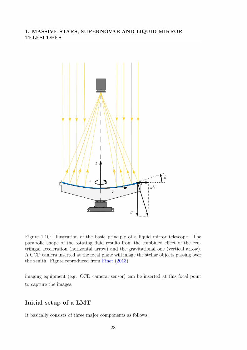
1. MASSIVE STARS, SUPERNOVAE AND LIQUID MIRRORTELESCOPES
Figure 1.10: Illustration of the basic principle of a liquid mirror telescope. Theparabolic shape of the rotating fluid results from the combined effect of the cen-trifugal acceleration (horizontal arrow) and the gravitational one (vertical arrow).A CCD camera inserted at the focal plane will image the stellar objects passing overthe zenith. Figure reproduced from Finet (2013).
imaging equipment (e.g. CCD camera, sensor) can be inserted at this focal point
to capture the images.
Initial setup of a LMT
It basically consists of three major components as follows:
28
1.3 Liquid mirror telescopes (LMTs)
• A dish container
- Initially, a large amount of mercury is poured to build up the mirror. With a
density of 13.534 g/cm3, mercury turns out to be a very heavy metal. There-
fore, a very stiff and light designed container is important. For the mirrors with
average aperture size, a simple dish spincast with epoxy or other polymer-resin
has sufficient stiffness.
• An air bearing system
- The optical quality of the liquid surface depends mainly on three parameters:
the Hg-air interface, vibrations and the vertical alignment of the rotation axis.
The third parameter implies that wobbling should be controlled accurately. A
search for the available technology (late 80’s) showed that only air-bearings
provided a sufficient angular stiffness, low friction and a precision compatible
with LMT requirements.
• A drive system
- This component of the mirror has undergone a major evolution in its design
since the first LMTs. The drive system has to be regular (precision better
than 10−6 ) and must not transmit vibrations to the mirror that would disturb
the surface.The first designs used a synchronous motor linked to a precise
oscillator. Previously, the mirror was driven by a belt over a pulley attached
to its base. This design was sufficient for a laboratory LMT but it was not
adapted for night observing conditions. The system suffered from moisture
and temperature variations.
1.3.3 Usefulness of LMTs
The technology advancements have led to construct several sophisticated large glass
mirror telescopes and presently, up to ∼10 m diameter telescopes are already con-
tributing to astronomical research. In the upcoming future, various ground based
giant-telescope projects are proposed (e.g. the Thirty Meter Telescope (TMT) and
the European Extremely Large Telescope (E-ELT)) projects1. However, LMTs have
some unique advantages over the glass mirror telescopes as described below.
1TMT is a 30m diameter telescope project while E-ELT is even larger than TMT consistingof a 39m diameter for the primary mirror; for more details on TMT and E-ELT see the respectivesites e.g. http://www.tmt.org/ and http://www.eso.org/public/teles-instr/e-elt/.
29
1. MASSIVE STARS, SUPERNOVAE AND LIQUID MIRRORTELESCOPES
• Inexpensive and simple design
The most important advantage of LMTs is its low cost. In comparison to glass
mirror telescopes, LMTs will cost an order of magnitude less for an equivalent
aperture (Borra, 1982). A 4m diameter glass telescope may cost more than
$100 millions, while similar diameter LMs will be very cheap, around $5 mil-
lions. More complicated designs of glass mirror will further increase the total
cost of these telescopes. Because of its very simple design, a small team of
people can run large LMTs working full-time on a specific project. Unlike the
traditional telescopes where a rotating dome is essential while the telescope
tracks stellar objects in different directions of the sky, the LMT dome struc-
ture is very simplified. Only a roll off roof is sufficient in a LMT enclosure
building.
• Easy maintenance
LMTs are low maintenance instruments. The complex tracking system of the
telescope and of a complex mirror support is not required in LMTs. Therefore,
maintenance is very easy. In case of glass mirror telescopes, when dust is
settled over the aluminized coating surface of the glass mirror, the telescope
is stopped and the mirror is removed from the tube. After that, several days
of precise work of mirror aluminizing starts. Once aluminizing is completed,
the next step begins with the alignment of the mirror. The whole process
of aluminizing and re-installing the mirrors kills several days up to one week
before new observations may start. In contrast to glass mirrors, the cleaning
of LMs is extremely simple. After a continuous run of 1-2 months, if the image
quality of a LMT degrades, the LM can be stopped to clean the mercury. The
complete process of cleaning and restarting the liquid mirror takes less than
one day.
• Optimal imaging position
Since the seeing and atmospheric transparency are best at zenith, LMTs are
mostly benefited with zenithal pointing. Therefore, images obtained with these
telescopes are of optimal quality. The image acquisition procedure in LMTs
(TDI mode, see Sect.5.2.4 for more details) are in such a way that stellar
images are formed by averaging the signal over the whole range of CCD rows.
Consequently, the image reduction is done by dividing each column by a one-
dimensional flat field.
30
1.3 Liquid mirror telescopes (LMTs)
• Continuous data acquisition
During the observations with traditional telescopes, a significant fraction of
the observing time is lost in slewing, making flat acquisition, waiting for the
readout time, etc. On the contrary, LMTs continuously observe each night
the same strip of sky without losing any time.
• Appropriate for survey programs
LMTs have the restriction to point towards the zenith only but these telescopes
are still very suitable for many survey programs (e.g. large-scale structure,
galaxy evolution, galaxy survey, long term photometric monitoring programs
etc.). As these kinds of survey programs are very much time consuming,
it is therefore not possible to get sufficient time on traditional telescopes to
properly carrying them out.
1.3.4 Major LMT observing facilities and their scientific
contributions
LMTs were initially developed for astronomical research. However, they have been
found to be useful in other fields of science, such as LIDAR science, atmospheric
science, optical testing and search for space debris. In the following section we
present some of the LMT facilities which were working till recently.
2.7 m UBC/Laval LMT
This LMT was jointly built by the Universities of British Columbia and Laval
(Canada). It had a 2048 × 2048 CCD detector to capture images over its field
of view. The primary scientific program of this project was to obtain spectral en-
ergy distributions of all objects in the survey area. The quasar survey program
using this telescope has been presented in Gibson & Hickson (1991). Hickson et al.
(1994) have reported the successful construction and operation of the UBC/Laval
LMT. The primary mirror and an image obtained are shown in Fig. 1.11.
3.0 m NODO LMT
The NASA Orbital Debris Observatory (NODO) project was located near Cloud-
croft in New Mexico. It was a three meter class LMT. This telescope was started
31
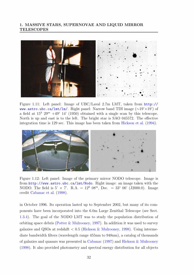
1. MASSIVE STARS, SUPERNOVAE AND LIQUID MIRRORTELESCOPES
Figure 1.11: Left panel: Image of UBC/Laval 2.7m LMT, taken from http://
www.astro.ubc.ca/lmt/lm/. Right panel: Narrow band TDI image (∼19’×19’) ofa field at 15h 29m +49 14’ (1950) obtained with a single scan by this telescope.North is up and east is to the left. The bright star is SAO 045572. The effectiveintegration time is 129 sec. This image has been taken from Hickson et al. (1994).
Figure 1.12: Left panel: Image of the primary mirror NODO telescope. Image isfrom http://www.astro.ubc.ca/lmt/Nodo. Right image: an image taken with theNODO. The field is 5’ × 7’. R.A. = 12h 08m, Dec. = 33 00’ (J2000.0). Imagecredit Cabanac et al. (1998).
in October 1996. Its operation lasted up to September 2002, but many of its com-
ponents have been incorporated into the 6.0m Large Zenithal Telescope (see Sect.
1.3.4). The goal of the NODO LMT was to study the population distribution of
orbiting space debris (Potter & Mulrooney, 1997). In addition it was used to survey
galaxies and QSOs at redshift < 0.5 (Hickson & Mulrooney, 1998). Using interme-
diate bandwidth filters (wavelength range 455nm to 948nm), a catalog of thousands
of galaxies and quasars was presented in Cabanac (1997) and Hickson & Mulrooney
(1998). It also provided photometry and spectral energy distribution for all objects
32
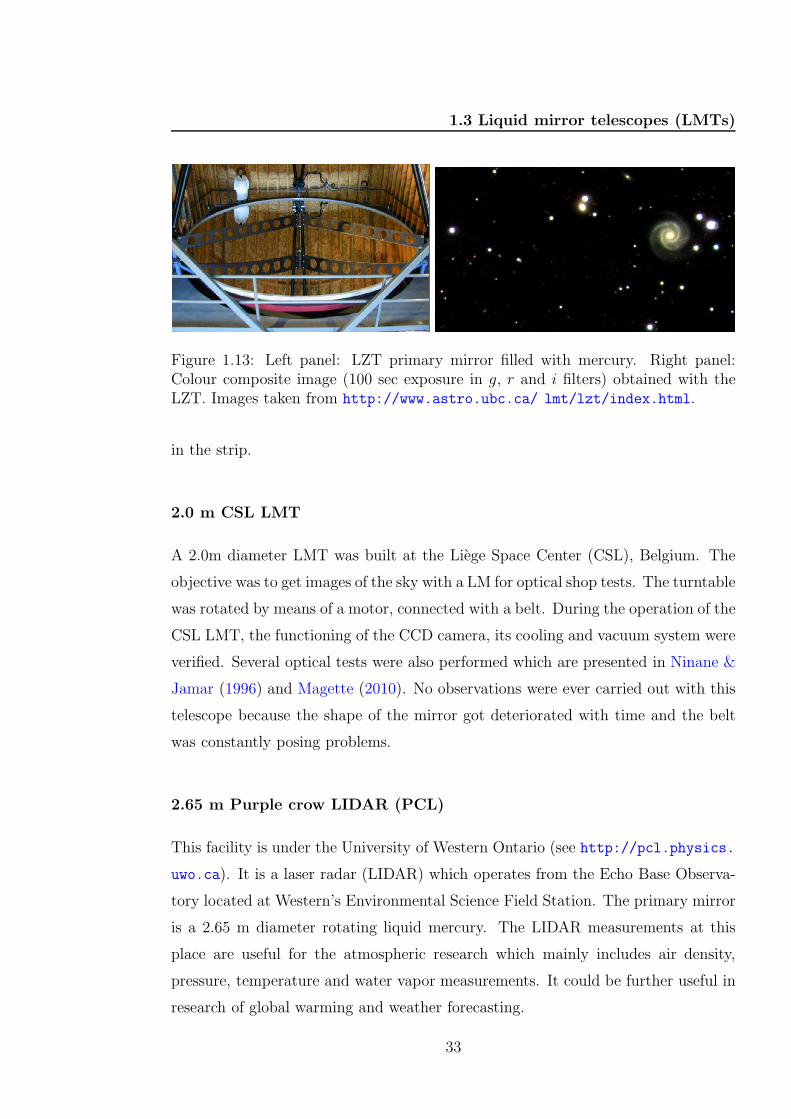
1.3 Liquid mirror telescopes (LMTs)
Figure 1.13: Left panel: LZT primary mirror filled with mercury. Right panel:Colour composite image (100 sec exposure in g, r and i filters) obtained with theLZT. Images taken from http://www.astro.ubc.ca/ lmt/lzt/index.html.
in the strip.
2.0 m CSL LMT
A 2.0m diameter LMT was built at the Liege Space Center (CSL), Belgium. The
objective was to get images of the sky with a LM for optical shop tests. The turntable
was rotated by means of a motor, connected with a belt. During the operation of the
CSL LMT, the functioning of the CCD camera, its cooling and vacuum system were
verified. Several optical tests were also performed which are presented in Ninane &
Jamar (1996) and Magette (2010). No observations were ever carried out with this
telescope because the shape of the mirror got deteriorated with time and the belt
was constantly posing problems.
2.65 m Purple crow LIDAR (PCL)
This facility is under the University of Western Ontario (see http://pcl.physics.
uwo.ca). It is a laser radar (LIDAR) which operates from the Echo Base Observa-
tory located at Western’s Environmental Science Field Station. The primary mirror
is a 2.65 m diameter rotating liquid mercury. The LIDAR measurements at this
place are useful for the atmospheric research which mainly includes air density,
pressure, temperature and water vapor measurements. It could be further useful in
research of global warming and weather forecasting.
33
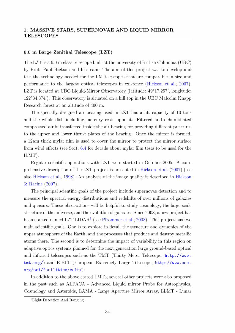
1. MASSIVE STARS, SUPERNOVAE AND LIQUID MIRRORTELESCOPES
6.0 m Large Zenithal Telescope (LZT)
The LZT is a 6.0 m class telescope built at the university of British Columbia (UBC)
by Prof. Paul Hickson and his team. The aim of this project was to develop and
test the technology needed for the LM telescopes that are comparable in size and
performance to the largest optical telescopes in existence (Hickson et al., 2007).
LZT is located at UBC Liquid-Mirror Observatory (latitude: 4917.257’, longitude:
12234.374’). This observatory is situated on a hill top in the UBC Malcolm Knapp
Research forest at an altitude of 400 m.
The specially designed air bearing used in LZT has a lift capacity of 10 tons
and the whole dish including mercury rests upon it. Filtered and dehumidiated
compressed air is transferred inside the air bearing for providing different pressures
to the upper and lower thrust plates of the bearing. Once the mirror is formed,
a 12µm thick mylar film is used to cover the mirror to protect the mirror surface
from wind effects (see Sect. 6.4 for details about mylar film tests to be used for the
ILMT).
Regular scientific operations with LZT were started in October 2005. A com-
prehensive description of the LZT project is presented in Hickson et al. (2007) (see
also Hickson et al., 1998). An analysis of the image quality is described in Hickson
& Racine (2007).
The principal scientific goals of the project include supernovae detection and to
measure the spectral energy distributions and redshifts of over millions of galaxies
and quasars. These observations will be helpful to study cosmology, the large-scale
structure of the universe, and the evolution of galaxies. Since 2008, a new project has
been started named LZT LIDAR1 (see Pfrommer et al., 2008). This project has two
main scientific goals. One is to explore in detail the structure and dynamics of the
upper atmosphere of the Earth, and the processes that produce and destroy metallic
atoms there. The second is to determine the impact of variability in this region on
adaptive optics systems planned for the next generation large ground-based optical
and infrared telescopes such as the TMT (Thirty Meter Telescope, http://www.
tmt.org/) and E-ELT (European Extremely Large Telescope, http://www.eso.
org/sci/facilities/eelt/).
In addition to the above stated LMTs, several other projects were also proposed
in the past such as ALPACA - Advanced Liquid mirror Probe for Astrophysics,
Cosmology and Asteroids, LAMA - Large Aperture Mirror Array, LLMT - Lunar
1LIght Detection And Ranging
34
1.3 Liquid mirror telescopes (LMTs)
Liquid Mirror Telescope (for more details visit http://www.astro.ubc.ca/lmt/
projects.html). Utilizing the emergence of the LM technology, a 4.0m LM project
(known as the International Liquid Mirror Telescope, ILMT) is in an advanced
stage. The first light of this telescope is expected in the year 2015. Part III of this
thesis is associated with it where we describe the design, construction, operational
experiments made with the ILMT and also present the current status of the telescope
site.
35


Part II
Massive stars and supernovae
37

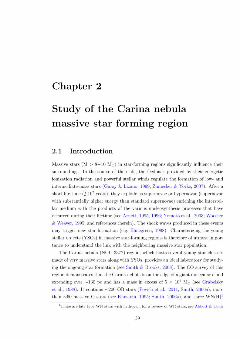
Chapter 2
Study of the Carina nebula
massive star forming region
2.1 Introduction
Massive stars (M > 8−10 M⊙) in star-forming regions significantly influence their
surroundings. In the course of their life, the feedback provided by their energetic
ionization radiation and powerful stellar winds regulate the formation of low- and
intermediate-mass stars (Garay & Lizano, 1999; Zinnecker & Yorke, 2007). After a
short life time (.107 years), they explode as supernovae or hypernovae (supernovae
with substantially higher energy than standard supernovae) enriching the interstel-
lar medium with the products of the various nucleosynthesis processes that have
occurred during their lifetime (see Arnett, 1995, 1996; Nomoto et al., 2003; Woosley
& Weaver, 1995, and references therein). The shock waves produced in these events
may trigger new star formation (e.g. Elmegreen, 1998). Characterizing the young
stellar objects (YSOs) in massive star-forming regions is therefore of utmost impor-
tance to understand the link with the neighboring massive star population.
The Carina nebula (NGC 3372) region, which hosts several young star clusters
made of very massive stars along with YSOs, provides an ideal laboratory for study-
ing the ongoing star formation (see Smith & Brooks, 2008). The CO survey of this
region demonstrates that the Carina nebula is on the edge of a giant molecular cloud
extending over ∼130 pc and has a mass in excess of 5 × 10⁵ M⊙ (see Grabelsky
et al., 1988). It contains ∼200 OB stars (Povich et al., 2011; Smith, 2006a), more
than ∼60 massive O stars (see Feinstein, 1995; Smith, 2006a), and three WN(H)1
1These are late type WN stars with hydrogen; for a review of WR stars, see Abbott & Conti
39
2. STUDY OF THE CARINA NEBULA MASSIVE STAR FORMINGREGION
Figure 2.1: Colour composite image of the large (2.7×2.7) area containing the Ca-rina Nebula and centered at α(J2000) = 10h 41m 17′′5 and δ(J2000) = −59 40′ 36′′9.This RGB image was made using the WISE 4.6 µm (red), 2MASS Ks band (green),and DSS R band (blue) images. Approximate locations of different star clusters(Tr 14, 15, 16; Bo 9, 10; Cr 228, 232, and NGC 3324) are denoted by white boxes. ηCarinae is marked by an arrow and in the lower left part of the image, south pillars(Smith et al., 2000) are seen. The region covered in the present study is shown bythe green box. Part of the selected field region can be seen in the extreme westernpart of the image. North is up and east is to the left. Image from Kumar et al.(2014b).
stars (i.e. WR 22, 24, and 25; Smith 2006a; Smith & Brooks 2008).
Initially, on the basis of infrared (IR) and molecular studies of the central Carina
(1987) and Crowther (2007).
40
2.1 Introduction
region, several authors (see Cox, 1995; de Graauw et al., 1981; Ghosh et al., 1988;
Harvey et al., 1979) have reported that the Carina nebula is an evolved Hii region
and that there is a paucity of active star formation. However, following the detection
of several embedded IR sources, Smith et al. (2000) showed that star formation is
still going on in this region. Later, Brooks et al. (2001) also identified two compact
Hii regions possibly linked with very young O-type stars. Rathborne et al. (2002)
traced the photodissociation regions (PDRs) that are expected to be present in the
massive star-forming regions. They conclude that the star formation within the Ca-
rina region has certainly not been completely halted despite prevailing unfavorable
conditions imposed by the very hot massive stars (see for more details Claeskens
et al., 2011). Detection of proplyds-like objects in these regions (see Dufour et al.,
1998; Smith et al., 2003) proves the ongoing active low- and intermediate-mass star
formation. Very recently, an isolated neutron star candidate discovered in the neigh-
borhood of η Carinae suggests there have been at least two episodes of massive star
formation (Hamaguchi et al., 2007; Pires et al., 2009).
Figure 2.1 shows a three-colour composite image, using the WISE 4.6 µm,
2MASS Ks band and DSS R band images, of the large region of the Carina nebula.
The prominent V-shaped lane is associated with the nebular complex and consists of
dust and molecular gas (Dickel, 1974). Trumpler (Tr) 16 is located near the central
portion of this lane and thought to be ∼3 Myr old. This cluster also hosts one of the
most massive stars in our galaxy, η Carinae (indicated by an arrow in the image),
which has an estimated initial mass & 150 M⊙ (Hillier et al., 2001). Tr 14 is younger
with an age of < 2Myr (Carraro et al., 2004; Smith & Brooks, 2008). In between
Tr 14 and Tr 16, there is another cluster named Collinder (Cr) 232. The cluster
Cr 228 near Tr 16 is very young and probably located in front of the Carina nebula
complex (Carraro & Patat, 2001). Finally NGC 3324 (upper part in the image) is
believed to be located inside the Carina spiral arm and embedded in a filamentary
elliptical shaped nebulosity (see Carraro et al., 2001).
Since the Carina nebula is a typical star-forming region, feedback from the young
and massive stars has cleared out the nebulosity in the central region and a large
number of elongated structures, so-called Pillars (Smith et al. 2000, seen in the lower
left part of the image) have formed in the outer regions. We can see many of them
in the southern part of the image. We also observe large bubbles in the northern
region, probably caused by the gusts of hot gas leaking from the powerful stars at
the center of the nebula (Smith et al., 2000). The central clusters Tr 14 and Tr 16
41
2. STUDY OF THE CARINA NEBULA MASSIVE STAR FORMINGREGION
tend to be devoid of star formation (Smith & Brooks, 2008), but there are active
sites of ongoing star formation in the outer regions of the nebula. In the present
study, our aim was to understand the star formation in one of the peripheral regions
of the Carina nebula, influenced by the presence of hot massive stars.
Because of its relatively low obscuration and proximity and its rich stellar con-
tent, this nebula is one of the most extensively explored nearby objects (Smith &
Brooks, 2008). Several wide-field surveys of the Carina Nebula complex (CNC) have
recently been carried out at different wavelengths. The combination of a large Chan-
dra X-ray survey (see Townsley et al., 2011) with a deep near-infrared (NIR) survey
(Preibisch et al., 2011c,d), Spitzer mid-infrared (MIR) observations (Povich et al.,
2011; Smith et al., 2010), and Herschel far-infrared (FIR) observations (Gaczkowski
et al., 2013; Roccatagliata et al., 2013) provides comprehensive information about
the young stellar populations. In the remainder, we discuss our new optical pho-
tometry, along with some low resolution spectroscopy, archival NIR (2MASS), and
X-ray (Chandra, XMM-Newton) data of a field located west of η Carinae (hereafter
CrW) and centered on the WN7ha + O binary system WR 22 (HD 92740; Conti
et al., 1979; Crowther et al., 1995; Gosset et al., 2009, 1991; Hamann et al., 1991;
Niemela, 1979; Rauw et al., 1996; van der Hucht et al., 1981) positioned just outside
the V-shaped dark lane.
2.2 Observations and data analysis
2.2.1 Optical photometry
A set of UBV RI and Hα observations of CrW (α(J2000) = 10h 41m 17′′5 and
δ(J2000) = −59 40′ 36′′9) were obtained with the Wide Field Imager (WFI) in-
strument at the ESO/MPG 2.2 m telescope at La Silla in March 2004 (service mode,
72.D-0093 PI: E. Gosset). The WFI instrument has a field of view of about 34′×33′,
covered by a mosaic of eight CCD chips with a pixel size of 0.238 arcsec. The ob-
servations typically consisted of three dithered frames with a short exposure time
(about 50s in U , 10s in BV RI, and 100s in Hα) and three dithered frames with
about 18 times longer exposures to allow measurements of both bright and faint
objects. Additional frames of a field located closer to the main Carina region were
also acquired in order to connect our photometric system to those of previous works.
42
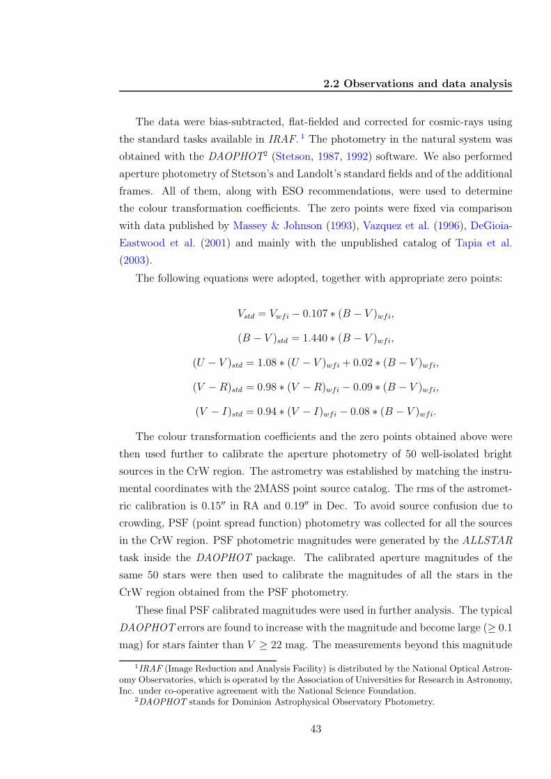
2.2 Observations and data analysis
The data were bias-subtracted, flat-fielded and corrected for cosmic-rays using
the standard tasks available in IRAF. 1 The photometry in the natural system was
obtained with the DAOPHOT2 (Stetson, 1987, 1992) software. We also performed
aperture photometry of Stetson’s and Landolt’s standard fields and of the additional
frames. All of them, along with ESO recommendations, were used to determine
the colour transformation coefficients. The zero points were fixed via comparison
with data published by Massey & Johnson (1993), Vazquez et al. (1996), DeGioia-
Eastwood et al. (2001) and mainly with the unpublished catalog of Tapia et al.
(2003).
The following equations were adopted, together with appropriate zero points:
Vstd = Vwfi − 0.107 ∗ (B − V )wfi,
(B − V )std = 1.440 ∗ (B − V )wfi,
(U − V )std = 1.08 ∗ (U − V )wfi + 0.02 ∗ (B − V )wfi,
(V −R)std = 0.98 ∗ (V − R)wfi − 0.09 ∗ (B − V )wfi,
(V − I)std = 0.94 ∗ (V − I)wfi − 0.08 ∗ (B − V )wfi.
The colour transformation coefficients and the zero points obtained above were
then used further to calibrate the aperture photometry of 50 well-isolated bright
sources in the CrW region. The astrometry was established by matching the instru-
mental coordinates with the 2MASS point source catalog. The rms of the astromet-
ric calibration is 0.15′′ in RA and 0.19′′ in Dec. To avoid source confusion due to
crowding, PSF (point spread function) photometry was collected for all the sources
in the CrW region. PSF photometric magnitudes were generated by the ALLSTAR
task inside the DAOPHOT package. The calibrated aperture magnitudes of the
same 50 stars were then used to calibrate the magnitudes of all the stars in the
CrW region obtained from the PSF photometry.
These final PSF calibrated magnitudes were used in further analysis. The typical
DAOPHOT errors are found to increase with the magnitude and become large (≥ 0.1
mag) for stars fainter than V ≥ 22 mag. The measurements beyond this magnitude
1IRAF (Image Reduction and Analysis Facility) is distributed by the National Optical Astron-omy Observatories, which is operated by the Association of Universities for Research in Astronomy,Inc. under co-operative agreement with the National Science Foundation.
2DAOPHOT stands for Dominion Astrophysical Observatory Photometry.
43
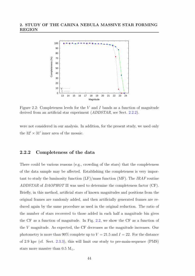
2. STUDY OF THE CARINA NEBULA MASSIVE STAR FORMINGREGION
0
10
20
30
40
50
60
70
80
90
100
13 14 15 16 17 18 19 20 21 22 23 24
Co
mp
lete
ne
ss (
%)
Magnitude
VI
Figure 2.2: Completeness levels for the V and I bands as a function of magnitudederived from an artificial star experiment (ADDSTAR, see Sect. 2.2.2).
were not considered in our analysis. In addition, for the present study, we used only
the 32′ × 31′ inner area of the mosaic.
2.2.2 Completeness of the data
There could be various reasons (e.g., crowding of the stars) that the completeness
of the data sample may be affected. Establishing the completeness is very impor-
tant to study the luminosity function (LF)/mass function (MF). The IRAF routine
ADDSTAR of DAOPHOT II was used to determine the completeness factor (CF).
Briefly, in this method, artificial stars of known magnitudes and positions from the
original frames are randomly added, and then artificially generated frames are re-
duced again by the same procedure as used in the original reduction. The ratio of
the number of stars recovered to those added in each half a magnitude bin gives
the CF as a function of magnitude. In Fig. 2.2, we show the CF as a function of
the V magnitude. As expected, the CF decreases as the magnitude increases. Our
photometry is more than 90% complete up to V = 21.5 and I = 22. For the distance
of 2.9 kpc (cf. Sect. 2.3.3), this will limit our study to pre-main-sequence (PMS)
stars more massive than 0.5 M⊙.
44
2.3 Basic parameters
2.2.3 Spectroscopy
For a set of 15 X-ray sources1 identified using XMM-Newton observations in the
CrW field (see Claeskens et al., 2011), we obtained their optical spectra between
4 and 6 March 2003 using the EMMI instrument mounted on the ESO 3.5 m New
Technology Telescope (NTT) at La Silla (PI: E. Gosset). This instrument was used
in the Red Imaging and Low Dispersion Spectroscopy (RILD) mode with grism
#5 (wavelength range 4000 - 8700 A). One spectrum was obtained with the VLT
+ FORS1 (see Claeskens et al., 2011). The data were reduced in the standard
way using the long context of the ESO-MIDAS (European Southern Observatory
Munich Image Data Analysis System) package2. Since the observing conditions were
favorable during our run, target spectra were calibrated using the flux spectrum of
the standard star LTT 2415 (Hamuy et al., 1992).
2.2.4 Archival data: 2MASS
We used the 2MASS Point Source Catalog (PSC) (Cutri et al., 2003) for NIR
(JHKs) photometry of point sources in the CrW region. This catalog is said to
be 99% complete up to the limiting magnitudes of 15.8, 15.1 and 14.3 in the J
(1.24µm), H (1.66µm), and Ks (2.16µm) bands, respectively3. We selected only
those sources that have a NIR photometric accuracy < 0.2 mag and detection in
at least the Ks and H bands. Since the seeing (∼FWHM of the stars intensity
profile) for the WFI observations was around 1 arcsec, the optical counterparts of
the 2MASS sources were searched using a matching radius of 1 arcsec.
2.3 Basic parameters
2.3.1 Reddening
The (U−B)/(B−V ) two-colour diagram (TCD) was used to estimate the extinction
toward the CrW region. In Fig. 2.3, we show the TCD with the zero-age-main-
sequence (ZAMS) from Schmidt-Kaler (1982) shifted along the reddening vector
with a slope of E(U − B)/E(B − V ) = 0.72 to match the observations. This shift
1Throughout this paper, we used the numbering convention of X-ray sources as introduced inClaeskens et al. (2011).
2ESO-MIDAS has been developed by the European Southern Observatory.3http://tdc-www.harvard.edu/catalogs/tmpsc.html
45
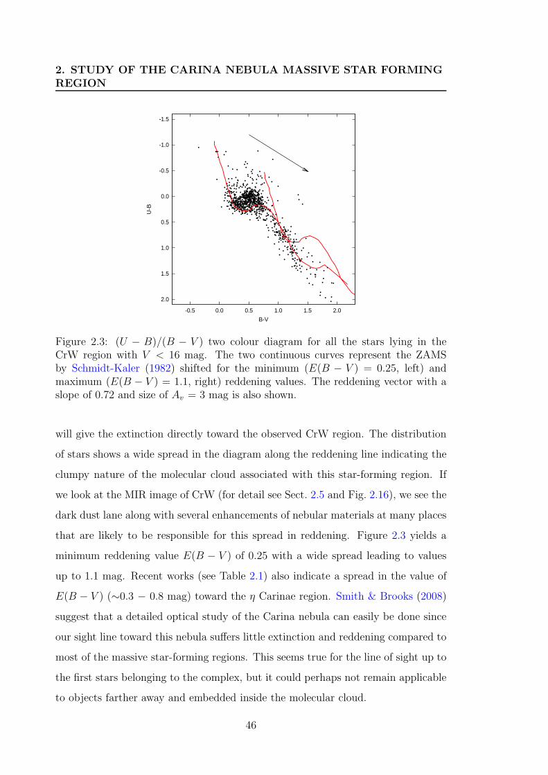
2. STUDY OF THE CARINA NEBULA MASSIVE STAR FORMINGREGION
-1.5
-1.0
-0.5
0.0
0.5
1.0
1.5
2.0
-0.5 0.0 0.5 1.0 1.5 2.0
U-B
B-V
Figure 2.3: (U − B)/(B − V ) two colour diagram for all the stars lying in theCrW region with V < 16 mag. The two continuous curves represent the ZAMSby Schmidt-Kaler (1982) shifted for the minimum (E(B − V ) = 0.25, left) andmaximum (E(B − V ) = 1.1, right) reddening values. The reddening vector with aslope of 0.72 and size of Av = 3 mag is also shown.
will give the extinction directly toward the observed CrW region. The distribution
of stars shows a wide spread in the diagram along the reddening line indicating the
clumpy nature of the molecular cloud associated with this star-forming region. If
we look at the MIR image of CrW (for detail see Sect. 2.5 and Fig. 2.16), we see the
dark dust lane along with several enhancements of nebular materials at many places
that are likely to be responsible for this spread in reddening. Figure 2.3 yields a
minimum reddening value E(B − V ) of 0.25 with a wide spread leading to values
up to 1.1 mag. Recent works (see Table 2.1) also indicate a spread in the value of
E(B − V ) (∼0.3 − 0.8 mag) toward the η Carinae region. Smith & Brooks (2008)
suggest that a detailed optical study of the Carina nebula can easily be done since
our sight line toward this nebula suffers little extinction and reddening compared to
most of the massive star-forming regions. This seems true for the line of sight up to
the first stars belonging to the complex, but it could perhaps not remain applicable
to objects farther away and embedded inside the molecular cloud.
46
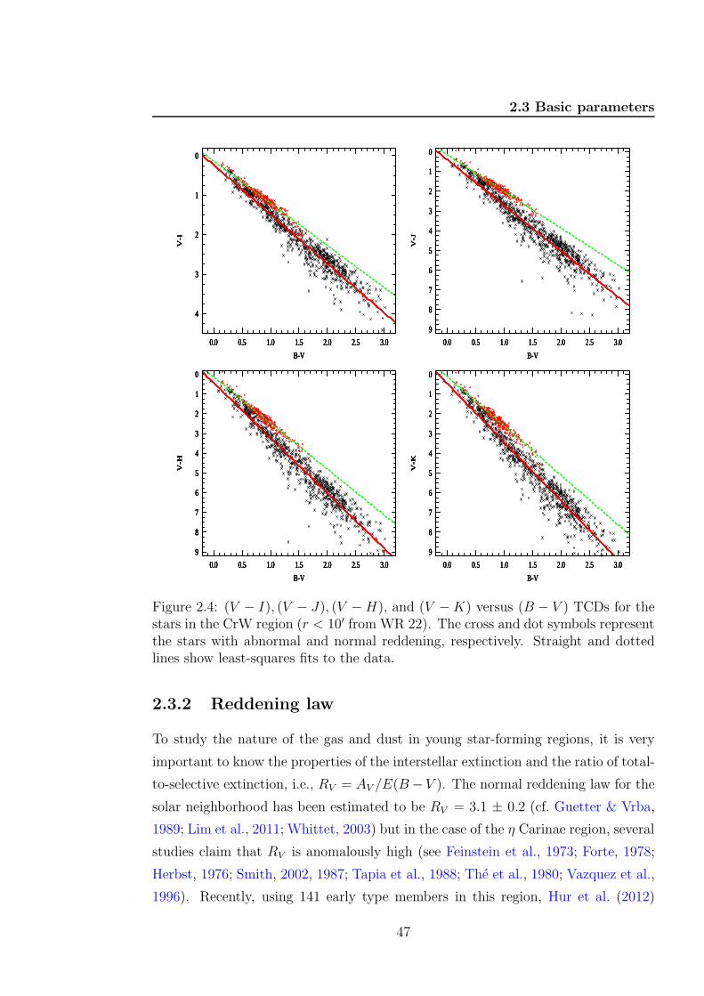
2.3 Basic parameters
0
1
2
3
4
0.0 0.5 1.0 1.5 2.0 2.5 3.0
V-I
B-V
0
1
2
3
4
0.0 0.5 1.0 1.5 2.0 2.5 3.0
V-I
B-V
0
1
2
3
4
0.0 0.5 1.0 1.5 2.0 2.5 3.0
V-I
B-V
0
1
2
3
4
0.0 0.5 1.0 1.5 2.0 2.5 3.0
V-I
B-V
0
1
2
3
4
5
6
7
8
9
0.0 0.5 1.0 1.5 2.0 2.5 3.0
V-J
B-V
0
1
2
3
4
5
6
7
8
9
0.0 0.5 1.0 1.5 2.0 2.5 3.0
V-J
B-V
0
1
2
3
4
5
6
7
8
9
0.0 0.5 1.0 1.5 2.0 2.5 3.0
V-J
B-V
0
1
2
3
4
5
6
7
8
9
0.0 0.5 1.0 1.5 2.0 2.5 3.0
V-J
B-V
0
1
2
3
4
5
6
7
8
9
0.0 0.5 1.0 1.5 2.0 2.5 3.0
V-H
B-V
0
1
2
3
4
5
6
7
8
9
0.0 0.5 1.0 1.5 2.0 2.5 3.0
V-H
B-V
0
1
2
3
4
5
6
7
8
9
0.0 0.5 1.0 1.5 2.0 2.5 3.0
V-H
B-V
0
1
2
3
4
5
6
7
8
9
0.0 0.5 1.0 1.5 2.0 2.5 3.0
V-H
B-V
0
1
2
3
4
5
6
7
8
9
0.0 0.5 1.0 1.5 2.0 2.5 3.0
V-K
B-V
0
1
2
3
4
5
6
7
8
9
0.0 0.5 1.0 1.5 2.0 2.5 3.0
V-K
B-V
0
1
2
3
4
5
6
7
8
9
0.0 0.5 1.0 1.5 2.0 2.5 3.0
V-K
B-V
0
1
2
3
4
5
6
7
8
9
0.0 0.5 1.0 1.5 2.0 2.5 3.0
V-K
B-V
Figure 2.4: (V − I), (V − J), (V −H), and (V −K) versus (B − V ) TCDs for thestars in the CrW region (r < 10′ from WR 22). The cross and dot symbols representthe stars with abnormal and normal reddening, respectively. Straight and dottedlines show least-squares fits to the data.
2.3.2 Reddening law
To study the nature of the gas and dust in young star-forming regions, it is very
important to know the properties of the interstellar extinction and the ratio of total-
to-selective extinction, i.e., RV = AV /E(B−V ). The normal reddening law for the
solar neighborhood has been estimated to be RV = 3.1 ± 0.2 (cf. Guetter & Vrba,
1989; Lim et al., 2011; Whittet, 2003) but in the case of the η Carinae region, several
studies claim that RV is anomalously high (see Feinstein et al., 1973; Forte, 1978;
Herbst, 1976; Smith, 2002, 1987; Tapia et al., 1988; The et al., 1980; Vazquez et al.,
1996). Recently, using 141 early type members in this region, Hur et al. (2012)
47
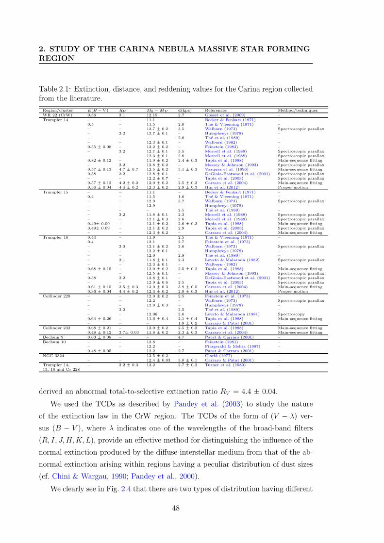
2. STUDY OF THE CARINA NEBULA MASSIVE STAR FORMINGREGION
Table 2.1: Extinction, distance, and reddening values for the Carina region collectedfrom the literature.
Region/cluster E(B − V ) RV M0 − MV d(kpc) References Method/techniquesWR 22 (CrW) 0.36 3.1 12.15 2.7 Gosset et al. (2009) –Trumpler 14 – – 11.1 – Becker & Fenkart (1971) –
0.5 – 11.5 2.0 The & Vleeming (1971) –– – 12.7 ± 0.2 3.5 Walborn (1973) Spectroscopic parallax– 3.2 12.7 ± 0.1 – Humphreys (1978) –– – – 2.8 The et al. (1980) –– – 12.3 ± 0.1 – Walborn (1982) –0.55 ± 0.08 – 12.2 ± 0.2 – Feinstein (1983) –– 3.2 12.7 ± 0.1 3.5 Morrell et al. (1988) Spectroscopic parallax– – 12.3 ± 0.1 2.8 Morrell et al. (1988) Spectroscopic parallax0.82 ± 0.12 – 11.9 ± 0.2 2.4 ± 0.3 Tapia et al. (1988) Main-sequence fitting– 3.2 12.8 ± 0.2 – Massey & Johnson (1993) Spectroscopic parallax0.57 ± 0.13 4.7 ± 0.7 12.5 ± 0.2 3.1 ± 0.3 Vazquez et al. (1996) Main-sequence fitting0.58 3.2 12.8 ± 0.1 – DeGioia-Eastwood et al. (2001) Spectroscopic parallax– – 12.2 ± 0.7 – Tapia et al. (2003) Spectroscopic parallax0.57 ± 0.12 4.2 ± 0.2 12.0 ± 0.2 2.5 ± 0.3 Carraro et al. (2004) Main-sequence fitting0.36 ± 0.04 4.4 ± 0.2 12.3 ± 0.2 2.9 ± 0.3 Hur et al. (2012) Proper motion
Trumpler 15 – – 11.1 – Becker & Fenkart (1971) –0.4 – 11.5 1.6 The & Vleeming (1971) –– – 12.9 3.7 Walborn (1973) Spectroscopic parallax– – 12.9 – Humphreys (1978) –– – – 2.5 The et al. (1980) –– 3.2 11.8 ± 0.1 2.3 Morrell et al. (1988) Spectroscopic parallax– – 12.1 ± 0.3 2.6 Morrell et al. (1988) Spectroscopic parallax0.49± 0.09 – 12.1 ± 0.2 2.6 ± 0.3 Tapia et al. (1988) Main-sequence fitting0.49± 0.09 – 12.1 ± 0.2 2.9 Tapia et al. (2003) Spectroscopic parallax– – 12.3 ± 0.2 – Carraro et al. (2004) Main-sequence fitting
Trumpler 16 0.44 – 11.9 2.5 The & Vleeming (1971) –0.4 – 12.1 2.7 Feinstein et al. (1973) –– 3.0 12.1 ± 0.2 2.6 Walborn (1973) Spectroscopic parallax– – 12.2 ± 0.1 – Humphreys (1978) –– – 12.0 2.8 The et al. (1980) –– 3.1 11.8 ± 0.1 2.3 Levato & Malaroda (1982) Spectroscopic parallax– – 12.3 ± 0.1 – Walborn (1982) –0.68 ± 0.15 – 12.0 ± 0.2 2.5 ± 0.2 Tapia et al. (1988) Main-sequence fitting– – 12.5 ± 0.1 – Massey & Johnson (1993) Spectroscopic parallax0.58 3.2 12.8 ± 0.1 – DeGioia-Eastwood et al. (2001) Spectroscopic parallax– – 12.0 ± 0.6 2.5 Tapia et al. (2003) Spectroscopic parallax0.61 ± 0.15 3.5 ± 0.3 13.0 ± 0.3 3.9 ± 0.5 Carraro et al. (2004) Main-sequence fitting0.36 ± 0.04 4.4 ± 0.2 12.3 ± 0.2 2.9 ± 0.3 Hur et al. (2012) Proper motion
Collinder 228 – – 12.0 ± 0.2 2.5 Feinstein et al. (1973) –– – 12.2 – Walborn (1973) Spectroscopic parallax– – 12.0 ± 0.3 – Humphreys (1978) –– 3.2 – 2.5 The et al. (1980) –– – 12.06 2.6 Levato & Malaroda (1981) Spectroscopy0.64 ± 0.26 – 11.6 ± 0.4 2.1 ± 0.4 Tapia et al. (1988) Main-sequence fitting– – – 1.9 ± 0.2 Carraro & Patat (2001) –
Collinder 232 0.68 ± 0.21 – 12.0 ± 0.2 2.5 ± 0.2 Tapia et al. (1988) Main-sequence fitting0.48 ± 0.12 3.7± 0.03 11.8 ± 0.2 2.3 ± 0.3 Carraro et al. (2004) Main-sequence fitting
Bochum 9 0.63 ± 0.08 – – 4.7 Patat & Carraro (2001) –Bochum 10 – – 12.8 – Feinstein (1981) –
– – 12.2 – Fitzgerald & Mehta (1987) –0.48 ± 0.05 – 12.2 2.7 Patat & Carraro (2001) –
NGC 3324 – – 12.5 ± 0.2 – Claria (1977) –– – 12.4 ± 0.03 3.0 ± 0.1 Carraro & Patat (2001) –
Trumpler 14, – 3.2 ± 0.3 12.2 2.7 ± 0.2 Turner et al. (1980) –15, 16 and Cr 228
derived an abnormal total-to-selective extinction ratio RV = 4.4 ± 0.04.
We used the TCDs as described by Pandey et al. (2003) to study the nature
of the extinction law in the CrW region. The TCDs of the form of (V − λ) ver-
sus (B − V ), where λ indicates one of the wavelengths of the broad-band filters
(R, I, J,H,K, L), provide an effective method for distinguishing the influence of the
normal extinction produced by the diffuse interstellar medium from that of the ab-
normal extinction arising within regions having a peculiar distribution of dust sizes
(cf. Chini & Wargau, 1990; Pandey et al., 2000).
We clearly see in Fig. 2.4 that there are two types of distribution having different
48
2.3 Basic parameters
slopes. We selected all the stars belonging to these two populations and plotted their
(V −I), (V −J), (V −H) and (V −K) vs. (B−V ) TCDs in Fig. 2.4. The respective
slopes relating these colours were found, for the red-dot stars, to be 1.07±0.02, 1.86±0.02, 2.33±0.03, and 2.50±0.03, which are approximately equivalent to the normal
galactic values, i.e., 1.10, 1.96, 2.42, and 2.60, respectively. The objects with black
crosses display steeper slopes, i.e., 1.28±0.01, 2.34±0.03, 2.84±0.03 and 3.03±0.03
for (V − I), (V − J), (V −H) and (V −K) vs. (B− V ), respectively. If we plot the
spatial distribution of the red dots and black crosses, we clearly see that all the red
dots are uniformly distributed, whereas all the black crosses are distributed away
from the obscured region of the molecular cloud. It means that the black crosses
are most probably background stars, and their light is seen through the molecular
cloud (see Preibisch et al., 2011a; Roccatagliata et al., 2013, and references therein).
Therefore, the ratios [E(V −λ)]/[E(B−V )] (λ ≥ λI) for the stars in the background
yield a high value for RV (∼3.7 ± 0.1), indicating an abnormal grain size in the
observed region. Many investigators (see column 3 of Table 2.1) have also found
evidence of larger dust grains in the Carina region. Marraco et al. (1993) have found
that the value of λmax (the wavelength at which maximum polarization occurred,
which is also an indicator of the mean dust grain size distribution) is higher than
the canonical value for the general diffuse ISM.
Several studies have already pointed toward an anomalous reddening law with a
high RV value in the vicinity of star-forming regions (see, e.g., Pandey et al., 2003).
However, for the Galactic diffuse interstellar medium, a normal value of RV = 3.1 is
well accepted. The higher-than-normal value of RV has usually been attributed to
the presence of larger dust grains. There is evidence that, within the dark clouds,
accretion of ice mantles on grains and coagulation due to colliding grains change
the size distribution towards larger particles. On the other hand, in star-forming
regions, radiation from massive stars may evaporate ice mantles resulting in small
particles. Here, it is interesting to mention that Okada et al. (2003) suggest that
efficient dust destruction is undergoing in the ionized region on the basis of the
[Si II] 35 to [N II] 122 µm ratio. Chini & Kruegel (1983) and Chini & Wargau
(1990) have shown that both larger and smaller grains may increase the ratio of
total-to-selective extinction.
49
2. STUDY OF THE CARINA NEBULA MASSIVE STAR FORMINGREGION
2.3.3 Distance
The Carina nebula is a very large (angular size > 2 × 1.5) active star-forming
region containing a number of young star clusters featuring very massive O-type
stars. Recently many authors have considered that the distance to η Carinae and
to the whole Carina region is 2.3 kpc (see, e.g., Povich et al., 2011; Smith, 2006b).
There is a large discrepancy in the measured distances to the clusters situated
within this nebula, as can be seen from Table 2.1. This large scatter in the distance
occurs because, as noted by Smith & Brooks (2008), the direction of the Galactic
plane in the Carina nebula nearly looks down the tangent point of the Sagittarius-
Carina spiral arm. The two clusters Tr 14 and Tr 16, located towards the center of
the Carina nebula, have been extensively studied by several authors, but the debate
about their distance is still open. Vazquez et al. (1996) estimated a distance modulus
of V0 −MV = 12.5 ± 0.2 mag for Tr 14. By applying an abnormal reddening law,
Tapia et al. (2003) derived V0−MV = 12.1 mag. In their study, they adopted AV =
1.39E(V − J) and found that both clusters are situated at the same distance. But
in another study, Carraro et al. (2004) concluded that both clusters are situated at
different distances with V0 −MV = 12.3 ± 0.2 mag for Tr 14 and 13.0 ± 0.3 mag
for Tr 16. Recently, Hur et al. (2012) concluded that Tr 14 and Tr 16 are at the
same distance within the observational errors (V0 − MV = 12.3 ± 0.2 mag, i.e., d
= 2.9 ± 0.3 kpc). Their derived distance is based upon the proper motion, which
is comparatively more accurate than other methods. Since we are concentrating on
the western side of the Carina nebula containing some part of Tr 14, for the present
study, we have adopted a distance of 2.9 kpc for CrW as given by Hur et al. (2012).
2.4 Results
2.4.1 Spectroscopically identified sources
The MK spectral types of 15 X-ray emitting sources in the CrW region have been
established using newly acquired spectra (see Sect. 2.2.3) and their comparison with
the digital spectral classification atlas compiled by R.O. Gray and available on the
web1. The results are summarized in Table 2.2, from which we may infer that the
majority of identified sources are late-type stars (see Fig. 2.5 for different spectral
types), and none of these stars features an Hα emission.
1http://www.ned.ipac.caltech.edu/level/Gray/frames.html
50
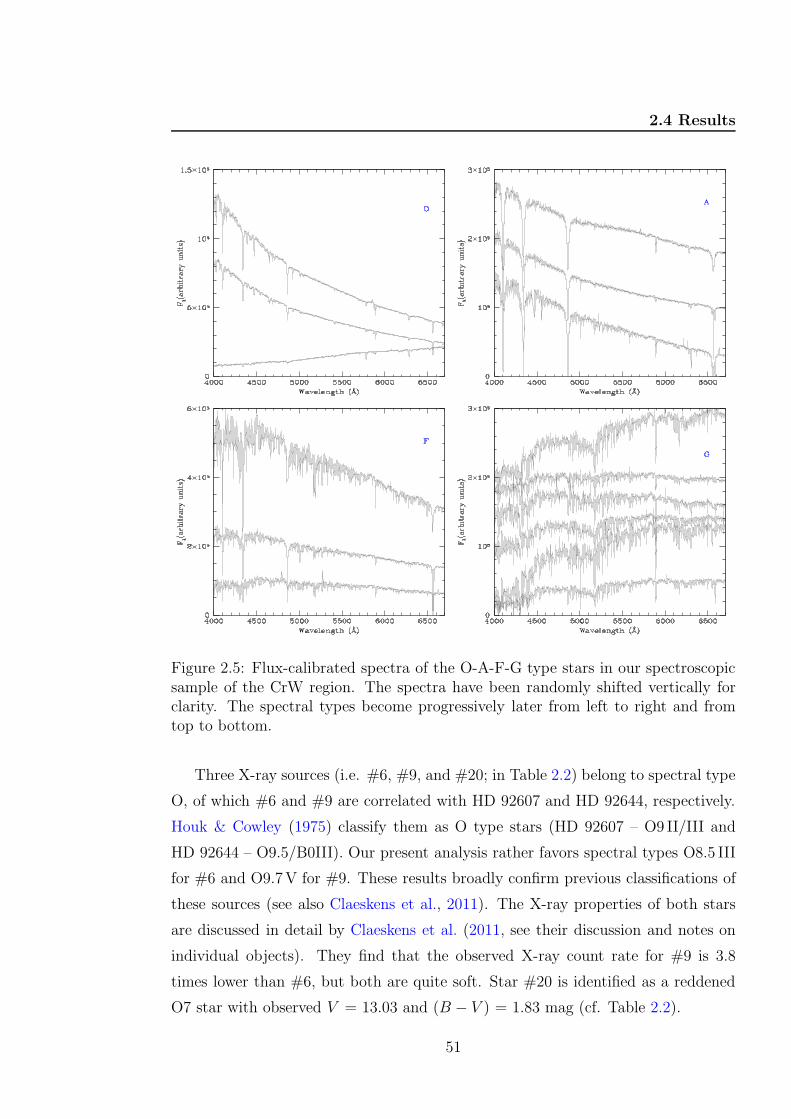
2.4 Results
Figure 2.5: Flux-calibrated spectra of the O-A-F-G type stars in our spectroscopicsample of the CrW region. The spectra have been randomly shifted vertically forclarity. The spectral types become progressively later from left to right and fromtop to bottom.
Three X-ray sources (i.e. #6, #9, and #20; in Table 2.2) belong to spectral type
O, of which #6 and #9 are correlated with HD 92607 and HD 92644, respectively.
Houk & Cowley (1975) classify them as O type stars (HD 92607 – O9 II/III and
HD 92644 – O9.5/B0III). Our present analysis rather favors spectral types O8.5 III
for #6 and O9.7V for #9. These results broadly confirm previous classifications of
these sources (see also Claeskens et al., 2011). The X-ray properties of both stars
are discussed in detail by Claeskens et al. (2011, see their discussion and notes on
individual objects). They find that the observed X-ray count rate for #9 is 3.8
times lower than #6, but both are quite soft. Star #20 is identified as a reddened
O7 star with observed V = 13.03 and (B − V ) = 1.83 mag (cf. Table 2.2).
51
2. STUDY OF THE CARINA NEBULA MASSIVE STAR FORMINGREGION
The remaining 12 sources have counterparts that are classified as late-type stars:
three are of spectral type A, three are F stars, and six are classified as G-type stars.
Stars #11, #19, and #37 are identified as A5 V, A1 III, and A1 V, respectively.
Similarly #3, #10, and #23 belong to F5 V, F8 V, and F3 V spectral types,
respectively. Claeskens et al. (2011) in their study found that source #18 is among
the brightest X-ray sources in this field; however, they could not identify any optical
counterpart for this object from the GSC2.2 catalog. Based on IR colours, they
computed the V band magnitude of this object to be in between 20.2 − 21.5. Later
on by visual inspection of Digital Sky Survey images, they found a star having
brightness V = 18 − 19 at the exact source location. We also found a star with
magnitude 18.214 ± 0.012 (cf. Table 2.2, column 4) at a similar position. Binarity
could explain why this star is brighter in the optical than expected from its near-IR
magnitudes (Claeskens et al., 2011). It could reside in front of the Carina, but it
could also be intrinsically brighter than a main-sequence (MS) star. Sources #7,
#12, #15, #32, #40, and #42 are characterized as G6 III, G9 V, G8 III, G3 V-III,
G8 V, and G9 III spectral type, respectively. Based on the observed X-ray counts,
Claeskens et al. (2011) claim that #42 is a variable star. It is also worthwhile to
mention that two sources (#7 and #15) are identified as PMS sources (see Table 2.2)
in the present study (cf. Sect. 2.4.2.3).
2.4.2 YSOs identification
The PMS stars (YSOs) are mainly grouped into the classes 0-I-II-III, which represent
in-falling protostars, evolved protostars, classical T-Tauri stars (CTTSs), and weak
line T Tauri stars (WTTSs), respectively (cf. Feigelson & Montmerle, 1999). Class
0 & I YSOs are so deeply buried inside the molecular clouds that they are not
visible at optical wavelengths. The CTTSs feature disks from which the material
is accreted, and emission in Hα can be seen as due to this accreting material.
These disks can also be probed through their IR excess (compared to normal stellar
photospheres). WTTSs, on the contrary, have little or no disk material left, hence
have no strong Hα emission and IR excess. It is evident from the recent studies
that the X-ray luminosity from WTTSs is significantly higher than for the CTTSs
with circumstellar disks or protostars with accreting envelopes (Prisinzano et al.,
2008; Stassun et al., 2004; Telleschi et al., 2007). In this section we report the
tentative identification of YSOs on the basis of their Hα emission, IR excess, and
X-ray emission.
52
2.4 Results
2.4.2.1 On the basis of Hα emission
The stars showing emission in Hα might be considered as PMS stars or candidates,
and the strength of the Hα line (measured by its equivalent width ‘EW(Hα)’) is a
direct indicator of their evolutionary stage. The conventional distinction between
CTTSs and WTTSs is an EW(Hα) > 10A for the former (see Herbig & Bell,
1988). However, Bertout (1989) has suggested that a limiting value of 5A might be
more appropriate. More recently, investigators have tied the definition to the shape
(width) of the Hα line profile (see Jayawardhana et al., 2003; White & Basri, 2003).
In the study of NGC 6383, Rauw et al. (2010) find that an Hα equivalent width of
10A corresponds to an (R−Hα) index of 0.24 ± 0.04 above the MS relation of Sung
et al. (1997). They have further used this as a selection criterion for identifying Hα
emitters. In our study, we have considered a source as probable Hα emitter only if
the (R −Hα) index is 0.24 above the MS relation by Sung et al. (1997).
The Hα filter at WFI has a special passband, therefore it cannot be directly
linked to any existing standard photometric system (see also Rauw et al., 2010).
By selecting ten stars observed with EMMI (see Sect. 2.2.3), whose spectra do not
exhibit Hα emission, we calibrated the zero point by comparing the observed R−Hα
and dereddened (V −I) with the (R−Hα)0 versus the (V −I)0 relation of emission
free MS stars as determined by Sung et al. (1997) for NGC 2264. The (V −I) colour
is dereddened by the E(V − I) value of E(B − V )min × 1.5. In Fig. 2.6, we plotted
the (R−Hα)0 vs. (V − I)0 distribution of all the stars along with the MS given by
Sung et al. (1997).
Since there is a large scatter in the distribution (cf. Fig. 2.6; left panel), there
may be false identifications ofHα emitters. To minimize this, we introduced another
selection criterion to identify the Hα emitters in addition to the previous one. We
used the V vs. (R − Hα)0 colour magnitude diagram (CMD) (cf. Fig. 2.6; right
panel) and defined an envelope that contains most of the stars following the MS.
The stars that have a value of (R−Hα)0−σ(R−Hα) greater than that of the envelope
of the MS can be assumed to be probable Hα emitters. In our study, we therefore
consider that a star is a good Hα emission candidate if it satisfies both conditions.
We have identified 41 YSOs in our study as potential Hα emitters, and these can
be seen in Fig. 2.16.
53
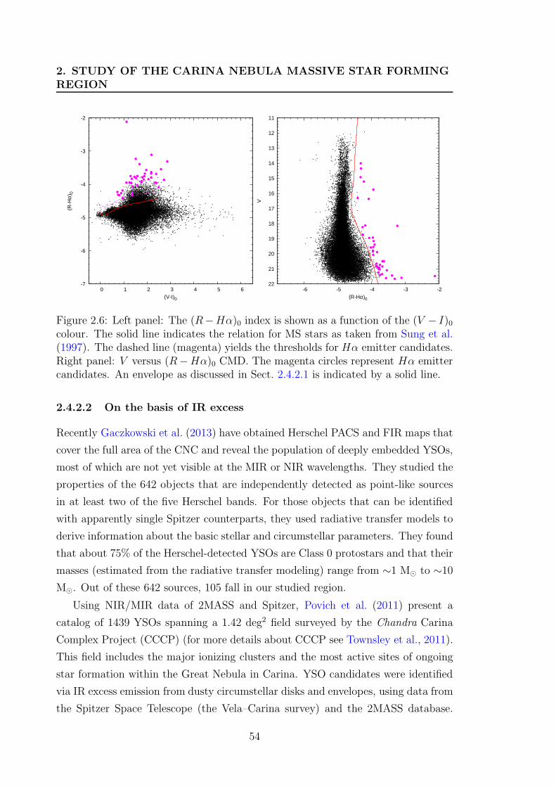
2. STUDY OF THE CARINA NEBULA MASSIVE STAR FORMINGREGION
-7
-6
-5
-4
-3
-2
0 1 2 3 4 5 6
(R-H
α)0
(V-I)0
11
12
13
14
15
16
17
18
19
20
21
22 -6 -5 -4 -3 -2
V
(R-Hα)0
Figure 2.6: Left panel: The (R−Hα)0 index is shown as a function of the (V − I)0colour. The solid line indicates the relation for MS stars as taken from Sung et al.(1997). The dashed line (magenta) yields the thresholds for Hα emitter candidates.Right panel: V versus (R−Hα)0 CMD. The magenta circles represent Hα emittercandidates. An envelope as discussed in Sect. 2.4.2.1 is indicated by a solid line.
2.4.2.2 On the basis of IR excess
Recently Gaczkowski et al. (2013) have obtained Herschel PACS and FIR maps that
cover the full area of the CNC and reveal the population of deeply embedded YSOs,
most of which are not yet visible at the MIR or NIR wavelengths. They studied the
properties of the 642 objects that are independently detected as point-like sources
in at least two of the five Herschel bands. For those objects that can be identified
with apparently single Spitzer counterparts, they used radiative transfer models to
derive information about the basic stellar and circumstellar parameters. They found
that about 75% of the Herschel-detected YSOs are Class 0 protostars and that their
masses (estimated from the radiative transfer modeling) range from ∼1 M⊙ to ∼10
M⊙. Out of these 642 sources, 105 fall in our studied region.
Using NIR/MIR data of 2MASS and Spitzer, Povich et al. (2011) present a
catalog of 1439 YSOs spanning a 1.42 deg2 field surveyed by the Chandra Carina
Complex Project (CCCP) (for more details about CCCP see Townsley et al., 2011).
This field includes the major ionizing clusters and the most active sites of ongoing
star formation within the Great Nebula in Carina. YSO candidates were identified
via IR excess emission from dusty circumstellar disks and envelopes, using data from
the Spitzer Space Telescope (the Vela–Carina survey) and the 2MASS database.
54
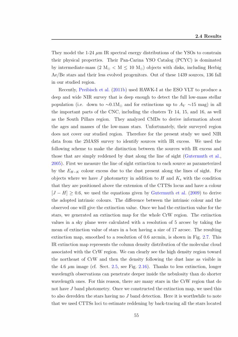
2.4 Results
They model the 1-24 µm IR spectral energy distributions of the YSOs to constrain
their physical properties. Their Pan-Carina YSO Catalog (PCYC) is dominated
by intermediate-mass (2 M⊙ < M ≤ 10 M⊙) objects with disks, including Herbig
Ae/Be stars and their less evolved progenitors. Out of these 1439 sources, 136 fall
in our studied region.
Recently, Preibisch et al. (2011b) used HAWK-I at the ESO VLT to produce a
deep and wide NIR survey that is deep enough to detect the full low-mass stellar
population (i.e. down to ∼0.1M⊙ and for extinctions up to AV ∼15 mag) in all
the important parts of the CNC, including the clusters Tr 14, 15, and 16, as well
as the South Pillars region. They analyzed CMDs to derive information about
the ages and masses of the low-mass stars. Unfortunately, their surveyed region
does not cover our studied region. Therefore for the present study we used NIR
data from the 2MASS survey to identify sources with IR excess. We used the
following scheme to make the distinction between the sources with IR excess and
those that are simply reddened by dust along the line of sight (Gutermuth et al.,
2005). First we measure the line of sight extinction to each source as parameterized
by the EH−K colour excess due to the dust present along the lines of sight. For
objects where we have J photometry in addition to H and Ks with the condition
that they are positioned above the extension of the CTTSs locus and have a colour
[J − H ] ≥ 0.6, we used the equations given by Gutermuth et al. (2009) to derive
the adopted intrinsic colours. The difference between the intrinsic colour and the
observed one will give the extinction value. Once we had the extinction value for the
stars, we generated an extinction map for the whole CrW region. The extinction
values in a sky plane were calculated with a resolution of 5 arcsec by taking the
mean of extinction value of stars in a box having a size of 17 arcsec. The resulting
extinction map, smoothed to a resolution of 0.6 arcmin, is shown in Fig. 2.7. This
IR extinction map represents the column density distribution of the molecular cloud
associated with the CrW region. We can clearly see the high density region toward
the northeast of CrW and then the density following the dust lane as visible in
the 4.6 µm image (cf. Sect. 2.5, see Fig. 2.16). Thanks to less extinction, longer
wavelength observations can penetrate deeper inside the nebulosity than do shorter
wavelength ones. For this reason, there are many stars in the CrW region that do
not have J band photometry. Once we constructed the extinction map, we used this
to also deredden the stars having no J band detection. Here it is worthwhile to note
that we used CTTSs loci to estimate reddening by back-tracing all the stars located
55
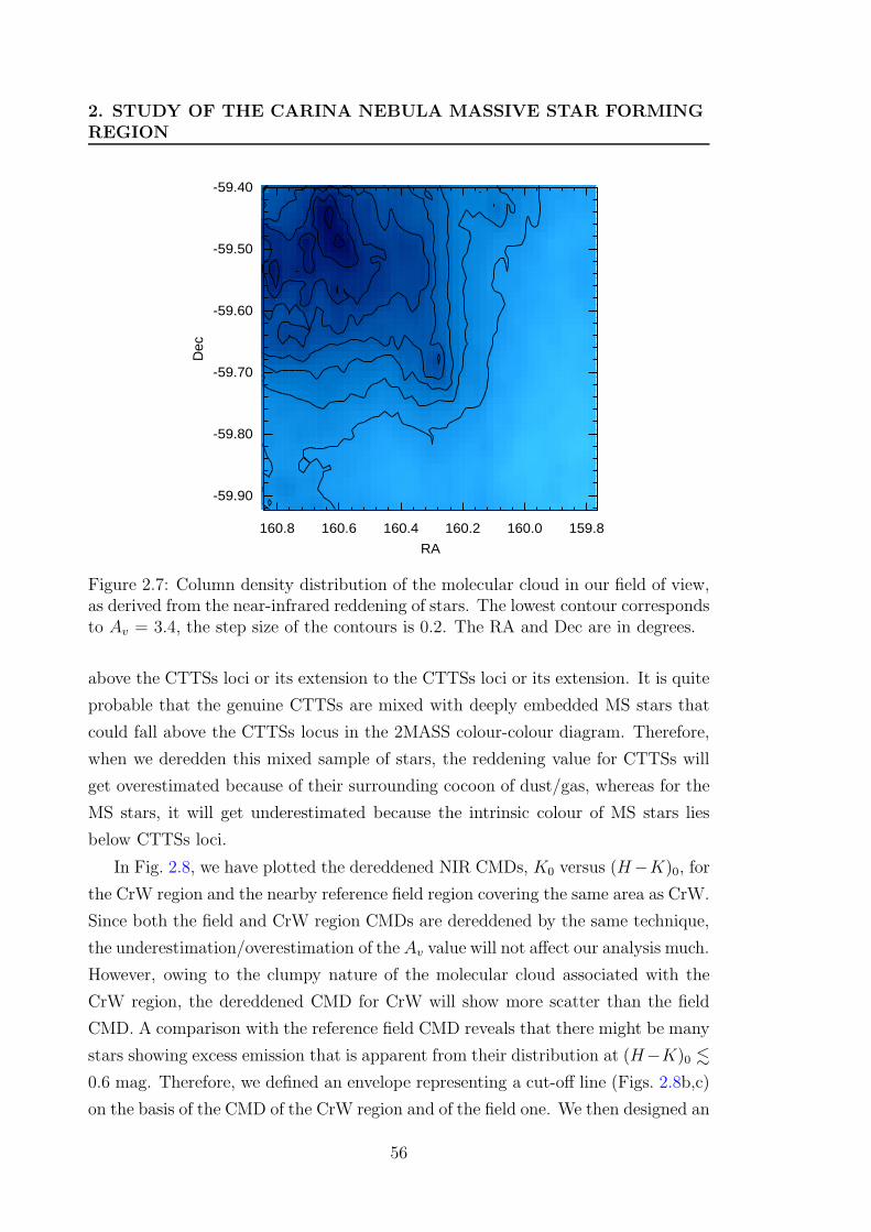
2. STUDY OF THE CARINA NEBULA MASSIVE STAR FORMINGREGION
159.8160.0160.2160.4160.6160.8
RA
-59.90
-59.80
-59.70
-59.60
-59.50
-59.40D
ec
Figure 2.7: Column density distribution of the molecular cloud in our field of view,as derived from the near-infrared reddening of stars. The lowest contour correspondsto Av = 3.4, the step size of the contours is 0.2. The RA and Dec are in degrees.
above the CTTSs loci or its extension to the CTTSs loci or its extension. It is quite
probable that the genuine CTTSs are mixed with deeply embedded MS stars that
could fall above the CTTSs locus in the 2MASS colour-colour diagram. Therefore,
when we deredden this mixed sample of stars, the reddening value for CTTSs will
get overestimated because of their surrounding cocoon of dust/gas, whereas for the
MS stars, it will get underestimated because the intrinsic colour of MS stars lies
below CTTSs loci.
In Fig. 2.8, we have plotted the dereddened NIR CMDs, K0 versus (H−K)0, for
the CrW region and the nearby reference field region covering the same area as CrW.
Since both the field and CrW region CMDs are dereddened by the same technique,
the underestimation/overestimation of the Av value will not affect our analysis much.
However, owing to the clumpy nature of the molecular cloud associated with the
CrW region, the dereddened CMD for CrW will show more scatter than the field
CMD. A comparison with the reference field CMD reveals that there might be many
stars showing excess emission that is apparent from their distribution at (H−K)0 .
0.6 mag. Therefore, we defined an envelope representing a cut-off line (Figs. 2.8b,c)
on the basis of the CMD of the CrW region and of the field one. We then designed an
56
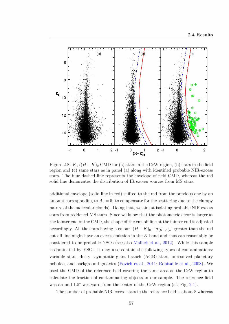
2.4 Results
Figure 2.8: K0/(H−K)0 CMD for (a) stars in the CrW region, (b) stars in the fieldregion and (c) same stars as in panel (a) along with identified probable NIR-excessstars. The blue dashed line represents the envelope of field CMD, whereas the redsolid line demarcates the distribution of IR excess sources from MS stars.
additional envelope (solid line in red) shifted to the red from the previous one by an
amount corresponding to Av = 5 (to compensate for the scattering due to the clumpy
nature of the molecular clouds). Doing that, we aim at isolating probable NIR excess
stars from reddened MS stars. Since we know that the photometric error is larger at
the fainter end of the CMD, the shape of the cut-off line at the fainter end is adjusted
accordingly. All the stars having a colour ‘(H−K)0−σ(H−K)0 ’ greater than the red
cut-off line might have an excess emission in the K band and thus can reasonably be
considered to be probable YSOs (see also Mallick et al., 2012). While this sample
is dominated by YSOs, it may also contain the following types of contaminations:
variable stars, dusty asymptotic giant branch (AGB) stars, unresolved planetary
nebulae, and background galaxies (Povich et al., 2011; Robitaille et al., 2008). We
used the CMD of the reference field covering the same area as the CrW region to
calculate the fraction of contaminating objects in our sample. The reference field
was around 1.5 westward from the center of the CrW region (cf. Fig. 2.1).
The number of probable NIR excess stars in the reference field is about 8 whereas
57
2. STUDY OF THE CARINA NEBULA MASSIVE STAR FORMINGREGION
0 1 2 3
0
1
2
3
H-K
Figure 2.9: (J − H)/(H − K) colour-colour diagram of sources detected in theJHKs bands in the CrW region. The sequences of dwarfs (solid curve) and giants(thick dashed curve) are from Bessell & Brett (1988). The dotted line represents thelocus of T Tauri stars (Meyer et al., 1997). Parallel dashed straight lines representthe reddening vectors (Cohen et al., 1981). The crosses on the dashed lines areseparated by AV = 5 mag. YSO candidates are also shown. Open magenta squares= Spitzer; filled magenta circles = Hα; filled squares = X-ray emitting WTTSs(green = XMM-Newton, blue = Chandra); open red triangles = CTTSs and opengreen circles = probable NIR-excess sources (see text for the classification scheme).
the number of probable NIR excess stars in the CrW region is 60. This means that
we have a contamination of about 13% in our sample. The majority of these probable
NIR excess stars follow the high density region in the CrW region (see Fig. 2.16)
and may be deeply embedded in that nebulosity. Povich et al. (2011) have identified
many YSOs that are mainly in the irradiated surface of the cloud (see Fig. 2.16)
but recently, based on Herschel FIR data, Gaczkowski et al. (2013) have identified
YSOs that are also located within the dark lane of the CrW region.
YSOs such as CTTSs, WTTSs, and Herbig Ae/Be stars tend to occupy differ-
ent regions on the NIR TCDs. In Fig. 2.9, we have plotted the NIR TCD using
58
2.4 Results
the 2MASS data for all the sources lying in the observed region. All the 2MASS
magnitudes and colours were converted into the California Institute of Technology
(CIT) system1. All the curves and lines are also in the CIT system. The shown
reddening vectors are drawn from the tip (spectral type M4) of the giant branch
(“upper reddening line”), from the base (spectral type A0) of the MS branch (“mid-
dle reddening line”) and from the tip of the intrinsic CTTSs line (“lower reddening
line”). The extinction ratios AJ/AV = 0.265, AH/AV = 0.155 and AK/AV = 0.090
have been taken from Cohen et al. (1981). We classified the sources according to
three regions in this diagram (cf. Ojha et al., 2004). The ‘F’ sources are located
between the upper and middle reddening lines and are considered to be either field
stars (MS stars, giants) or Class III and Class II sources with small NIR-excess. ‘T’
sources are located between the middle and lower reddening lines. These sources are
considered to be mostly CTTSs (or Class II objects) with large NIR-excess. There
may be an overlap of Herbig Ae/Be stars in the ‘T’ region (Hillenbrand et al., 1992).
‘P’ sources are those located in the region redward of the lower reddening line and
are most likely Class 0/I objects (protostellar-like objects; Ojha et al. (2004)). It is
worthwhile also mentioning that Robitaille et al. (2006) show that there is a signifi-
cant overlap between protostars and CTTSs. The NIR TCD of the observed region
(Fig. 2.9) indicates that a significant number of sources that have previously been
identified as probable NIR-excess stars lie in the ‘T’ region. Forty-one sources have
been designated as CTTSs in our study under the condition that they fall in the ‘T’
region of the NIR TCD (Fig. 2.9) and are redward of the dashed blue cut-off line in
the dereddened CMD (Fig. 2.8). We also have plotted probable NIR excess sources
that are detected in ‘J ’ band (10 out of 60). Most of these sources are located in
the ‘P’ region in Fig. 2.9, which means that they are most likely Class 0/I objects.
2.4.2.3 On the basis of X-ray emission
The NIR-excess-selected YSO candidate samples are generally considered incom-
plete because the NIR-excess emission in young stars disappears on timescales of
just a few Myr (see Briceno et al., 2007). At an age of ∼3 Myr, only ∼50% of the
young stars still show NIR excesses, and by ∼5 Myr this fraction is reduced to ∼15%
(Preibisch et al., 2011c). Since the expected ages of most young stars in the CNC
are several Myr, any IR-excess-selected YSO sample will be highly incomplete. To
1http://www.astro.caltech.edu/~jmc/2mass/v3/transformations/
59
2. STUDY OF THE CARINA NEBULA MASSIVE STAR FORMINGREGION
tackle this problem, we used the X-ray emitting point sources in the region to iden-
tify YSO candidates. The X-ray detection methods are sensitive to young stars that
have already dispersed their circumstellar disks, thus avoiding the bias introduced
when selecting samples only based on IR excess (Preibisch et al., 2011c).
XMM-Newton observations
The XMM-Newton satellite has observed the CrW region in the course of the study
of the massive binary WR 22. The corresponding results have been presented in
separate papers (see Claeskens et al., 2011; Gosset et al., 2009). In this section we
cross-correlated the sources detected in our photometric data of the CrW region
with the positions of 43 X-ray sources from Claeskens et al. (2011). The positions of
the X-ray sources as given by Claeskens et al. (2011, columns 8 and 9 of their table
2) refer to the astrometric frame as determined from the XMM-Newton on-board
Attitude and Orbit Control System. The cross-correlation with the GSC and the
present optical catalog suggests making a small correction. We therefore suggest
decreasing the right ascension of Claeskens et al. (2011) by 0′′.25 and increasing the
declination by 0′′.96. No rotation was detected. We adopt these new positions for
the 43 X-ray sources.
We defined an optimal cross-correlation radius to find a compromise between
correlations missed due to astrometric errors and spurious associations in the CrW
field. To derive the optimal correlation radius, we applied the technique of Jeffries
et al. (1997). In this method, the distribution of the cumulative number of cataloged
sources as a function of the cross-correlation radius rc is given by
Φ(d ≤ rc) =A
[
1− exp
(−r2c2 σ2
)]
+ (N −A)[
1− exp(−π B r2c )]
. (2.1)
In this equation N , A, σ, and B represent the total number of cross-correlated
X-ray sources (N = 43), the number of true correlations, the uncertainty in the
X-ray source position, and the surface density of the catalog of photometric sources,
respectively. In the course of fitting the integrated number of correlations with the
CrW photometric catalog as a function of the separation (where 43 X-ray sources
have an optical source located closer than 8 arcsec), we derived the fitting parameters
as A = 33.78, σ = 0.9 arcsec, and B = 2.3 × 10⁻² arcsec−2 (see Fig. 2.10). The
optimal correlation radius was chosen to be rc = 2.7 ′′, which implies that there is
60
2.4 Results
0 1 2 3 4 5 6 70
5
10
15
20
25
30
35
40
45
Cross correlation radius
Cum
ula
tive
num
ber
Figure 2.10: Cumulative numbers of correlations between the X-ray detected sourcesand the WFI catalog. The thick curve represents the observed numbers, the dashedcurve shows the best fit, and the dot-dashed line (magenta) and dotted (red) curvescorrespond to the expected numbers of real and spurious sources, respectively. Thevertical line indicates the optimal correlation radius rc.
no more than one spurious association among the 34 correlations; i.e., the optical
counterparts of 79% of the XMM-Newton sources in the CrW field should thus be
reliably identified.
Claeskens et al. (2011) also cross-correlated these X-ray sources (N = 43), but
they searched the optical counterparts using the Guide Star Catalog version 2.2
(GSC2.2). Their fitting parameters are A = 35.4, B = 2 × 10⁻³ arcsec−2, and
σ = 1.8 arcsec. The number of true correlations (A) of both studies are very much
consistent. The surface density (B) of the catalog of optical sources in the present
study is an order of magnitude higher than in Claeskens et al. (2011), while our σ
value is half that of these authors. The results of the cross-identification are listed
in Table 2.2. When several optical counterparts are present, only the closest one is
given. The first column is the ID of the X-ray sources from Claeskens et al. (2011).
Columns 2 and 3 are their respective RA and Dec in degree (from our photometric
catalog). In the next columns the V magnitude, (V − I), (V − R), (B − V ) and
(U − B) colours are reported. Sources with a spectral classification are mentioned
61
2. STUDY OF THE CARINA NEBULA MASSIVE STAR FORMINGREGION
Table 2.2: Cross-identification of 43 X-ray sources from Claeskens et al. (2011) withCrW optical photometry. Stars brighter than V = 11.3 are from the literature. TheYSOs identified in Section 2.4.2 are also mentioned in the last column.
ID(X-ray) α(J2000) δ(J2000) V (V − I) (V − R) (B − V ) (U − B) Spectral YSOtype number†
#1 159.894496 -59.737510 20.386 2.860 1.438 2.250 N/A – 183#2 159.947016 -59.608981 12.991 0.809 0.436 0.653 -0.042 – –#3 159.948029 -59.746218 10.470 N/A N/A 0.440 N/A F5V –#4 159.983333 -59.618056 11.279 N/A N/A 0.668 N/A – –#5 160.042973 -59.619011 17.720 2.299 1.195 1.721 1.051 – 57#6 160.051779 -59.802809 8.140 N/A N/A -0.020 -0.780 O8.5 III –#7 160.069977 -59.534346 14.720 1.386 0.787 1.006 0.673 G6 III 13#8 – – – – – – – – –#9 160.132138 -59.778854 8.880 N/A N/A -0.030 -0.900 O9.7V –#10 160.161981 -59.462519 12.839 0.807 0.419 0.590 0.028 F8V –#11 160.174252 -59.621872 12.609 0.429 0.258 0.320 0.108 A5V –#12 160.174412 -59.539547 14.974 0.954 0.540 0.736 0.149 G9V –#13 160.184003 -59.826372 17.565 3.222 1.551 2.103 1.018 – –#14 160.193248 -59.700809 19.680 2.144 1.115 1.544 N/A – –#15 160.214424 -59.622191 15.365 1.332 0.716 1.109 0.609 G8 III 18#16 – – – – – – – – –#17 160.229239 -59.639602 17.422 1.552 0.835 1.217 0.607 – 48#18 160.230446 -59.710999 18.214 1.586 0.928 1.086 0.373 F8V –#19 160.235367 -59.862561 11.363 0.340 N/A N/A N/A A1 III –#20 160.247070 -59.457005 13.031 1.825 0.860 1.340 -0.031 O7 –#21 – – – – – – – – –#22a 160.322983 -59.676915 6.420 N/A N/A 0.080 -0.730 – –#23 160.335850 -59.589894 11.692 0.718 N/A 0.841 -0.285 F3V –#24 160.338038 -59.659587 17.131 1.316 0.758 0.978 0.259 – –#25 – – – – – – – – –#26 160.362639 -59.656561 16.698 1.334 0.774 0.896 0.494 – –#27 160.364564 -59.686933 16.339 1.174 0.658 0.903 0.215 – –#28 160.387108 -59.604288 19.416 2.737 1.136 1.667 N/A – –#29 160.426017 -59.635431 16.982 1.335 0.712 1.054 0.482 – –#30 160.437963 -59.807270 19.050 2.058 0.922 1.818 N/A – –#31 160.464076 -59.720771 12.626 0.782 0.442 0.550 -0.019 – –#32 160.478811 -59.689836 13.146 1.224 0.793 0.935 0.923 G3V-III –#33 – – – – – – – – –#34 – – – – – – – – –#35 – – – – – – – – –#36 – – – – – – – – –#37 160.523400 -59.604232 14.022 0.554 0.316 0.357 0.158 A1V –#38 160.556738 -59.599388 18.204 2.910 1.446 2.081 0.479 – 87#39 160.564481 -59.565945 19.215 2.738 1.145 1.679 N/A – –#40 160.603836 -59.669004 14.842 1.105 0.636 0.576 0.164 G8 V –#41 160.636112 -59.611374 16.242 1.834 0.975 1.461 1.079 – 30#42 160.652591 -59.731771 15.372 1.454 0.764 1.096 0.746 G9 III –#43 160.679111 -59.591296 15.898 1.365 0.738 1.165 0.425 – –
a WR 22 itself; †The YSO entry numbers are from Table 2.3, see also Appendix 8.
in the next-to-last column.
Chandra X-ray observations
Recently, a wide area (1.42 deg2) of the Carina complex has been mapped by the
Chandra X-ray Observatory (CCCP, Townsley et al., 2011). These images were
obtained with the Advanced CCD Imaging Spectrometer (ACIS; Garmire et al.,
62
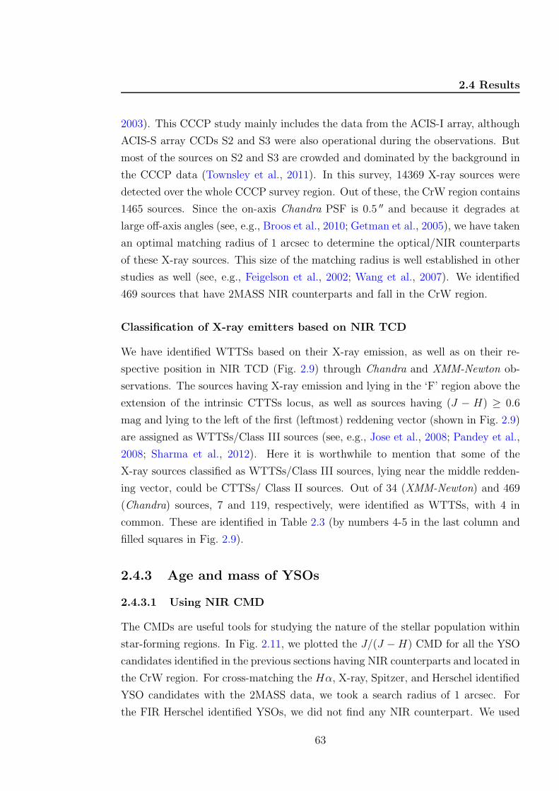
2.4 Results
2003). This CCCP study mainly includes the data from the ACIS-I array, although
ACIS-S array CCDs S2 and S3 were also operational during the observations. But
most of the sources on S2 and S3 are crowded and dominated by the background in
the CCCP data (Townsley et al., 2011). In this survey, 14369 X-ray sources were
detected over the whole CCCP survey region. Out of these, the CrW region contains
1465 sources. Since the on-axis Chandra PSF is 0.5 ′′ and because it degrades at
large off-axis angles (see, e.g., Broos et al., 2010; Getman et al., 2005), we have taken
an optimal matching radius of 1 arcsec to determine the optical/NIR counterparts
of these X-ray sources. This size of the matching radius is well established in other
studies as well (see, e.g., Feigelson et al., 2002; Wang et al., 2007). We identified
469 sources that have 2MASS NIR counterparts and fall in the CrW region.
Classification of X-ray emitters based on NIR TCD
We have identified WTTSs based on their X-ray emission, as well as on their re-
spective position in NIR TCD (Fig. 2.9) through Chandra and XMM-Newton ob-
servations. The sources having X-ray emission and lying in the ‘F’ region above the
extension of the intrinsic CTTSs locus, as well as sources having (J − H) ≥ 0.6
mag and lying to the left of the first (leftmost) reddening vector (shown in Fig. 2.9)
are assigned as WTTSs/Class III sources (see, e.g., Jose et al., 2008; Pandey et al.,
2008; Sharma et al., 2012). Here it is worthwhile to mention that some of the
X-ray sources classified as WTTSs/Class III sources, lying near the middle redden-
ing vector, could be CTTSs/ Class II sources. Out of 34 (XMM-Newton) and 469
(Chandra) sources, 7 and 119, respectively, were identified as WTTSs, with 4 in
common. These are identified in Table 2.3 (by numbers 4-5 in the last column and
filled squares in Fig. 2.9).
2.4.3 Age and mass of YSOs
2.4.3.1 Using NIR CMD
The CMDs are useful tools for studying the nature of the stellar population within
star-forming regions. In Fig. 2.11, we plotted the J/(J −H) CMD for all the YSO
candidates identified in the previous sections having NIR counterparts and located in
the CrW region. For cross-matching the Hα, X-ray, Spitzer, and Herschel identified
YSO candidates with the 2MASS data, we took a search radius of 1 arcsec. For
the FIR Herschel identified YSOs, we did not find any NIR counterpart. We used
63
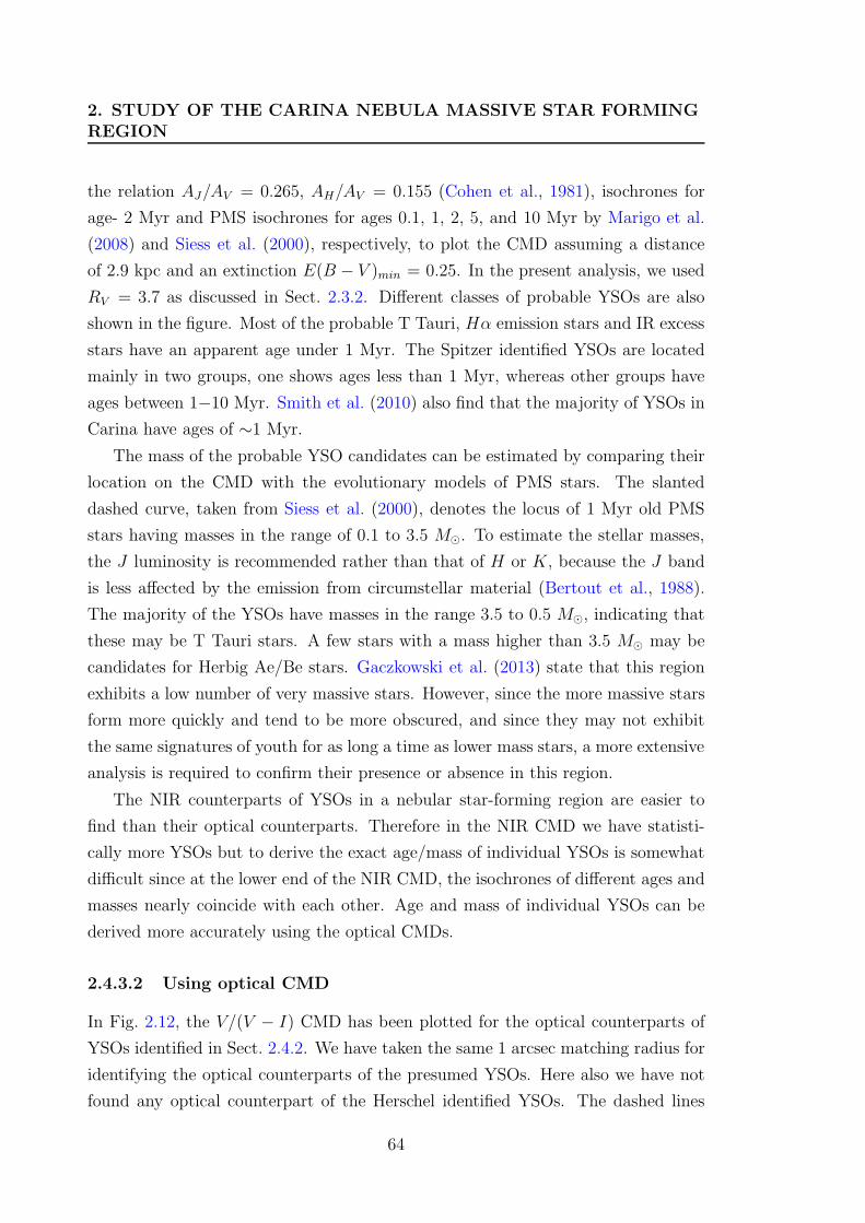
2. STUDY OF THE CARINA NEBULA MASSIVE STAR FORMINGREGION
the relation AJ/AV = 0.265, AH/AV = 0.155 (Cohen et al., 1981), isochrones for
age- 2 Myr and PMS isochrones for ages 0.1, 1, 2, 5, and 10 Myr by Marigo et al.
(2008) and Siess et al. (2000), respectively, to plot the CMD assuming a distance
of 2.9 kpc and an extinction E(B − V )min = 0.25. In the present analysis, we used
RV = 3.7 as discussed in Sect. 2.3.2. Different classes of probable YSOs are also
shown in the figure. Most of the probable T Tauri, Hα emission stars and IR excess
stars have an apparent age under 1 Myr. The Spitzer identified YSOs are located
mainly in two groups, one shows ages less than 1 Myr, whereas other groups have
ages between 1−10 Myr. Smith et al. (2010) also find that the majority of YSOs in
Carina have ages of ∼1 Myr.
The mass of the probable YSO candidates can be estimated by comparing their
location on the CMD with the evolutionary models of PMS stars. The slanted
dashed curve, taken from Siess et al. (2000), denotes the locus of 1 Myr old PMS
stars having masses in the range of 0.1 to 3.5 M⊙. To estimate the stellar masses,
the J luminosity is recommended rather than that of H or K, because the J band
is less affected by the emission from circumstellar material (Bertout et al., 1988).
The majority of the YSOs have masses in the range 3.5 to 0.5 M⊙, indicating that
these may be T Tauri stars. A few stars with a mass higher than 3.5 M⊙ may be
candidates for Herbig Ae/Be stars. Gaczkowski et al. (2013) state that this region
exhibits a low number of very massive stars. However, since the more massive stars
form more quickly and tend to be more obscured, and since they may not exhibit
the same signatures of youth for as long a time as lower mass stars, a more extensive
analysis is required to confirm their presence or absence in this region.
The NIR counterparts of YSOs in a nebular star-forming region are easier to
find than their optical counterparts. Therefore in the NIR CMD we have statisti-
cally more YSOs but to derive the exact age/mass of individual YSOs is somewhat
difficult since at the lower end of the NIR CMD, the isochrones of different ages and
masses nearly coincide with each other. Age and mass of individual YSOs can be
derived more accurately using the optical CMDs.
2.4.3.2 Using optical CMD
In Fig. 2.12, the V/(V − I) CMD has been plotted for the optical counterparts of
YSOs identified in Sect. 2.4.2. We have taken the same 1 arcsec matching radius for
identifying the optical counterparts of the presumed YSOs. Here also we have not
found any optical counterpart of the Herschel identified YSOs. The dashed lines
64
2.4 Results
0 1 2 3
18
16
14
12
10
8
6
J-H
G9
K1.5
K4
K5.5M0M5
Figure 2.11: J/(J − H) CMD for the stars in the CrW region. The isochrone of2 Myr (Z = 0.02) by Marigo et al. (2008) and PMS isochrones of age 0.1, 1, 2, 5and 10 Myr taken from Siess et al. (2000) corrected for a distance of 2.9 kpc anda reddening E(B − V )min = 0.25 are also shown. The symbols are the same as inFig. 2.9 (see Sect. 2.4.3.1 for the classification scheme). The indicated masses andspectral types have been taken from the 1 Myr PMS isochrone of Siess et al. (2000).
Table 2.3: Sample of the optically identified YSO candidates along with their derivedages and masses. Error bars in magnitude and colour represent formal internal(comparative) errors and do not include the colour transformation and zero-pointuncertainties.
ID α(J2000) δ(J2000) V ± σ (V − I)± σ Age ±σ Mass ±σ Technique() () (mag) (mag) (Myrs) (M⊙) 1,2,3,4,5,6
(1) (2) (3) (4) (5) (6) (7) (8)1 160.544858 -59.643538 12.316±0.009 0.373±0.018 0.9±0.2 3.7±0.2 12 160.586232 -59.898926 12.726±0.011 0.211±0.018 2.6±2.1 4.8±0.3 13 160.556561 -59.735036 13.079±0.011 0.422±0.014 1.4±0.2 2.8±0.3 14 159.827622 -59.759030 13.508±0.006 0.677±0.010 2.5±0.4 2.0±0.3 15 160.509158 -59.674841 13.527±0.009 1.000±0.014 1.4±0.2 3.4±0.3 1– – – – – – – –
1 Spitzer identified sources, 2 Hα sources, 3 CTTS, 4 Chandra sources, 5 XMM-Newton sources, 6 Probable NIRexcess
(This table is fully available in Appendix 8)
65
2. STUDY OF THE CARINA NEBULA MASSIVE STAR FORMINGREGION
Figure 2.12: V/(V − I) CMD for all the detected YSOs (symbols as in Fig. 2.9,see Sect. 2.4.2.2 for details). The isochrone for 2 Myr by Marigo et al. (2008)(continuous line) and PMS isochrones for 1, 2, 5, and 10 Myr by Siess et al. (2000)(dashed lines) are also shown. All the isochrones are corrected for a distance of 2.9kpc and reddening E(B−V ) = 0.25. The horizontal line with an arrow correspondsto the completeness limit of the observations.
(for different ages 0.1, 0.5, 1, 2, 5 and 10 Myr) show PMS isochrones by Siess et al.
(2000) and the post-main-sequence isochrone (continuous line) for 2 Myr by Marigo
et al. (2008). These isochrones are corrected for the CrW distance (2.9 kpc) and
minimum reddening (E(B − V ) = 0.25 mag, see previous section). It is clear from
Fig. 2.12 that a majority of the sources have ages < 1 Myr with a possible age
spread up to 10 Myr.
The age and mass of the YSOs have been derived using the V/(V − I) CMD.
The Siess et al. (2000) isochrones have very coarse resolution (30 points over their
whole mass range of 0.1 to 7 M⊙); therefore, for a better estimation of mass, these
isochrones were interpolated (2000 points). We used photometric errors along with
the error in the distance modulus and reddening to draw an error box around each
66
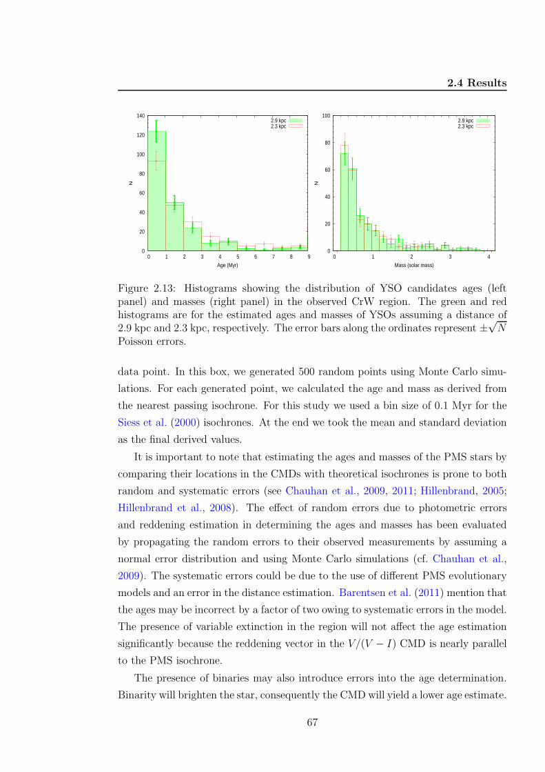
2.4 Results
0
20
40
60
80
100
120
140
0 1 2 3 4 5 6 7 8 9
N
Age (Myr)
2.9 kpc2.3 kpc
0
20
40
60
80
100
0 1 2 3 4
N
Mass (solar mass)
2.9 kpc2.3 kpc
Figure 2.13: Histograms showing the distribution of YSO candidates ages (leftpanel) and masses (right panel) in the observed CrW region. The green and redhistograms are for the estimated ages and masses of YSOs assuming a distance of2.9 kpc and 2.3 kpc, respectively. The error bars along the ordinates represent ±
√N
Poisson errors.
data point. In this box, we generated 500 random points using Monte Carlo simu-
lations. For each generated point, we calculated the age and mass as derived from
the nearest passing isochrone. For this study we used a bin size of 0.1 Myr for the
Siess et al. (2000) isochrones. At the end we took the mean and standard deviation
as the final derived values.
It is important to note that estimating the ages and masses of the PMS stars by
comparing their locations in the CMDs with theoretical isochrones is prone to both
random and systematic errors (see Chauhan et al., 2009, 2011; Hillenbrand, 2005;
Hillenbrand et al., 2008). The effect of random errors due to photometric errors
and reddening estimation in determining the ages and masses has been evaluated
by propagating the random errors to their observed measurements by assuming a
normal error distribution and using Monte Carlo simulations (cf. Chauhan et al.,
2009). The systematic errors could be due to the use of different PMS evolutionary
models and an error in the distance estimation. Barentsen et al. (2011) mention that
the ages may be incorrect by a factor of two owing to systematic errors in the model.
The presence of variable extinction in the region will not affect the age estimation
significantly because the reddening vector in the V/(V − I) CMD is nearly parallel
to the PMS isochrone.
The presence of binaries may also introduce errors into the age determination.
Binarity will brighten the star, consequently the CMD will yield a lower age estimate.
67
2. STUDY OF THE CARINA NEBULA MASSIVE STAR FORMINGREGION
In the case of an equal-mass binary, we expect an error of∼50% to ∼60% in the PMS
age estimation. However, it is difficult to estimate the influence of binaries/variables
on the mean age estimation because the fraction of binaries/variables is not known.
In the study of TTSs in the Hii region IC 1396, Barentsen et al. (2011) point out
that the number of binaries in their sample of TTSs could be very low since close
binaries lose their disk significantly faster than single stars (cf. Bouwman et al.,
2006).
We have calculated ages and masses for 241 optically identified individual YSO
candidates classified using different schemes (see Table 2.3). Here we would like to
point out that out of six optically identified probable NIR excess stars, five have
ages .1 Myr. They may be YSOs that are deeply embedded and are formed by
the collapse of the core of a molecular cloud. Estimated ages and masses of the
YSOs range from ∼0.1 to 10 Myr and ∼0.3 to 4.8 M⊙, respectively. This age range
indicates a wide spread in the formation of stars in the region. The histograms of
age and mass distribution of YSOs are shown in Fig. 2.13.
As stated in Sect. 2.3.3, several authors have used different distances (2.3 kpc)
than ours (2.9 kpc) for the Carina nebula. Therefore, we also examined the above
results (ages and masses of YSOs) for the distance of 2.3 kpc. The ages and masses
of YSOs are once again derived using the same procedure as described above and
the corresponding histograms are overplotted in Fig. 2.13. As can be seen in this
figure, both derived values are more or less similar within their corresponding errors,
although there are slight differences in the numbers of YSOs that are less than 1
Myr. By looking at this figure, we can safely conclude that the majority of the
YSOs are younger than 1 Myr and have a mass lower than 2 M⊙. These age and
mass are comparable with the lifetime and mass of TTSs.
2.4.4 Initial mass function
The distribution of stellar masses that formed in one star-formation event in a given
volume of space is called the initial mass function (IMF), and together with the
star formation rate, the IMF dictates the evolution and fate of galaxies and star
clusters. The effects of environment may be more revealing at the low-mass end of
the IMF, since one might imagine that the lower end of the mass spectrum is most
strongly affected by external effects. The goals of this study are to identify the PMS
populations in order to study the IMF down to the substellar regime.
68
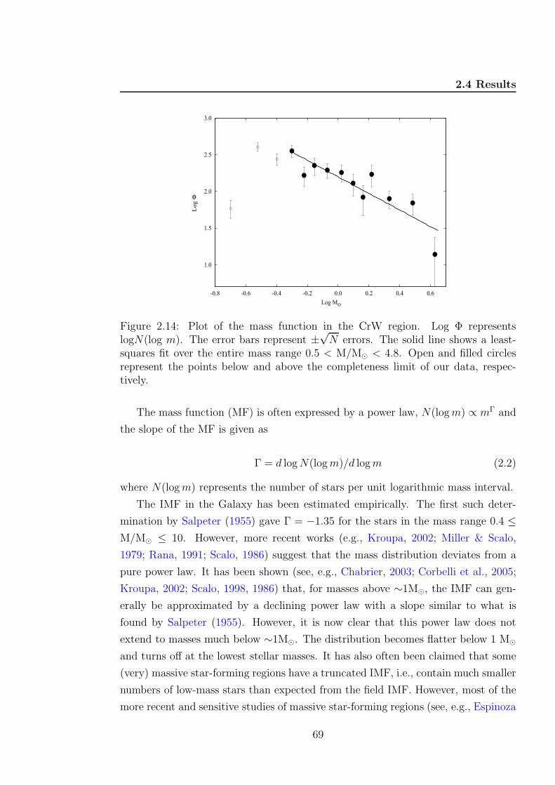
2.4 Results
1.0
1.5
2.0
2.5
3.0
-0.8 -0.6 -0.4 -0.2 0.0 0.2 0.4 0.6
Lo
g Φ
Log MO·
Figure 2.14: Plot of the mass function in the CrW region. Log Φ representslogN(log m). The error bars represent ±
√N errors. The solid line shows a least-
squares fit over the entire mass range 0.5 < M/M⊙ < 4.8. Open and filled circlesrepresent the points below and above the completeness limit of our data, respec-tively.
The mass function (MF) is often expressed by a power law, N(logm) ∝ mΓ and
the slope of the MF is given as
Γ = d logN(logm)/d logm (2.2)
where N(logm) represents the number of stars per unit logarithmic mass interval.
The IMF in the Galaxy has been estimated empirically. The first such deter-
mination by Salpeter (1955) gave Γ = −1.35 for the stars in the mass range 0.4 ≤M/M⊙ ≤ 10. However, more recent works (e.g., Kroupa, 2002; Miller & Scalo,
1979; Rana, 1991; Scalo, 1986) suggest that the mass distribution deviates from a
pure power law. It has been shown (see, e.g., Chabrier, 2003; Corbelli et al., 2005;
Kroupa, 2002; Scalo, 1998, 1986) that, for masses above ∼1M⊙, the IMF can gen-
erally be approximated by a declining power law with a slope similar to what is
found by Salpeter (1955). However, it is now clear that this power law does not
extend to masses much below ∼1M⊙. The distribution becomes flatter below 1 M⊙
and turns off at the lowest stellar masses. It has also often been claimed that some
(very) massive star-forming regions have a truncated IMF, i.e., contain much smaller
numbers of low-mass stars than expected from the field IMF. However, most of the
more recent and sensitive studies of massive star-forming regions (see, e.g., Espinoza
69
2. STUDY OF THE CARINA NEBULA MASSIVE STAR FORMINGREGION
et al., 2009; Liu et al., 2009) find the numbers of low-mass stars in agreement with
the expectation from the “normal” field star IMF. Preibisch et al. (2011c) confirm
these results for the Carina Nebula and support the assumption of a universal IMF
(at least in our Galaxy). In consequence, this result also supports the notion that
OB associations and very massive star clusters are the dominant formation sites of
the galactic field star population, as already suggested by Miller & Scalo (1978).
We have optically identified 241 YSO candidates (cf. Sect. 2.4.2) in the region of
CrW and then calculated their masses (cf. Sect. 2.4.3) with the help of optical CMD
using the theoretical PMS of Siess et al. (2000). Here we would like to mention that
for our photometry, the completeness limit is 0.5 M⊙ for a distance of 2.9 kpc. The
MF of the CrW region is plotted in Fig. 2.14. The slope of the MF ‘Γ’ in the mass
range 0.5 < M/M⊙ < 4.8 comes out to be −1.13 ± 0.20, which is a bit shallower
than the value given by Salpeter (1955), and there seems to be no break in the
slope at M ∼1 M⊙, as has been noticed in previous works (Jose et al., 2008; Pandey
et al., 2008; Sharma et al., 2007). On the other hand, Preibisch et al. (2011c) show
that, down to a mass limit around 0.5 − 1 M⊙, the shape of the IMF in Carina is
consistent with that in Orion (and thus the field IMF). Their results directly show
that there is clearly no deficit of low-mass stars in the CNC down to ∼1M⊙.
2.4.5 K-band luminosity function
The K-band luminosity function (KLF) represents the number of stars as a function
of the K-band magnitude. It is frequently used in studies of young clusters and star-
forming regions as a diagnostic tool of the mass function and the star formation
history of their stellar populations. The interpretation of KLF has been presented
by several authors (see, e.g., Lada & Lada, 2003; Muench et al., 2000; Zinnecker
et al., 1993, and references therein).
To obtain the KLF, it is essential to take the incompleteness of the data and the
foreground and background source contaminations into account. The completeness
of the data is estimated using the ADDSTAR routine of DAOPHOT as described
in Section 2.2.2. To consider the foreground/background field star contaminations,
we used both the Besancon Galactic model of stellar population synthesis (Robin
et al., 2003) and the nearby reference field stars. Star counts are predicted using
the Besancon model in the direction of the control field. We checked the validity
of the simulated model by comparing the model KLF with that of the control field
and found that both KLFs match rather well. An advantage to using the model is
70
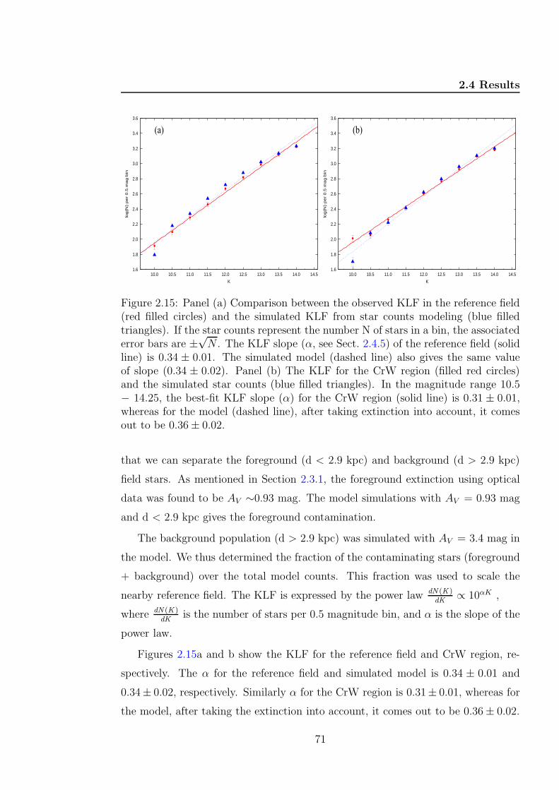
2.4 Results
1.6
1.8
2.0
2.2
2.4
2.6
2.8
3.0
3.2
3.4
3.6
10.0 10.5 11.0 11.5 12.0 12.5 13.0 13.5 14.0 14.5
log(N
) per
0.5
mag b
in
K
(a)
1.6
1.8
2.0
2.2
2.4
2.6
2.8
3.0
3.2
3.4
3.6
10.0 10.5 11.0 11.5 12.0 12.5 13.0 13.5 14.0 14.5
log(N
) per
0.5
mag b
in
K
(b)
Figure 2.15: Panel (a) Comparison between the observed KLF in the reference field(red filled circles) and the simulated KLF from star counts modeling (blue filledtriangles). If the star counts represent the number N of stars in a bin, the associatederror bars are ±
√N . The KLF slope (α, see Sect. 2.4.5) of the reference field (solid
line) is 0.34 ± 0.01. The simulated model (dashed line) also gives the same valueof slope (0.34 ± 0.02). Panel (b) The KLF for the CrW region (filled red circles)and the simulated star counts (blue filled triangles). In the magnitude range 10.5− 14.25, the best-fit KLF slope (α) for the CrW region (solid line) is 0.31 ± 0.01,whereas for the model (dashed line), after taking extinction into account, it comesout to be 0.36± 0.02.
that we can separate the foreground (d < 2.9 kpc) and background (d > 2.9 kpc)
field stars. As mentioned in Section 2.3.1, the foreground extinction using optical
data was found to be AV ∼0.93 mag. The model simulations with AV = 0.93 mag
and d < 2.9 kpc gives the foreground contamination.
The background population (d > 2.9 kpc) was simulated with AV = 3.4 mag in
the model. We thus determined the fraction of the contaminating stars (foreground
+ background) over the total model counts. This fraction was used to scale the
nearby reference field. The KLF is expressed by the power law dN (K )dK
∝ 10αK ,
where dN (K )dK
is the number of stars per 0.5 magnitude bin, and α is the slope of the
power law.
Figures 2.15a and b show the KLF for the reference field and CrW region, re-
spectively. The α for the reference field and simulated model is 0.34 ± 0.01 and
0.34± 0.02, respectively. Similarly α for the CrW region is 0.31± 0.01, whereas for
the model, after taking the extinction into account, it comes out to be 0.36± 0.02.
71
2. STUDY OF THE CARINA NEBULA MASSIVE STAR FORMINGREGION
2.5 Discussion: star formation scenario in the CrW
region
Povich et al. (2011) using Spitzer MIR data identified 1439 YSOs (Pan Carina YSO
Catalog) in the field surveyed by the CCCP. The spatial distribution of these YSOs
throughout the Carina Nebula shows a highly complex structure with clustering
at several positions. The majority of YSOs identified by them are located inside
the Hii cavities near, but less frequently within, the boundaries of dense molecular
clouds and the ends of the pillars. They also found that the high concentration of
the intermediate mass YSOs is in Tr 14 itself. They have concluded that the recent
star formation history in the Carina Nebula has been driven or at least regulated
by feedback from the massive stars.
Recently, Gaczkowski et al. (2013) identified 642 YSOs in the Carina Complex
with the help of FIR Herschel data. These YSOs are also found to be highly hetero-
geneously distributed in the region, and they do not follow the distribution of cloud
mass. Gaczkowski et al. (2013) show that the Herschel selected YSO candidates are
located near the irradiated surfaces of clouds (see Fig. 2.16) and pillars, whereas the
Spitzer selected ‘YSO’ candidates (Povich et al., 2011) often surround these pillars.
This characteristic spatial distribution of the young stellar populations in different
evolutionary stages has been related by Gaczkowski et al. (2013) to the idea that
the advancing ionization fronts compress the clouds and lead to cloud collapse and
star formation in these clouds, just ahead of the ionization fronts. They further
state that some fraction of the cloud mass is transformed into stars (and these are
the YSOs detected by Herschel), while another fraction of the cloud material is dis-
persed by the process of photo-evaporation. As time proceeds, the pillars shrink,
and a population of slightly older YSOs is left behind and revealed after the passage
of the ionization front. Their results provide additional evidence that the formation
of these YSOs was indeed triggered by the advancing ionization fronts of the massive
stars as suggested by the theoretical models (see Gritschneder et al., 2010).
Roccatagliata et al. (2013) with the help of the wide-field Herschel SPIRE and
PACS maps, determined the temperatures, surface densities, and the local strength
of the far-UV irradiation for all the cloud structures over the entire spatial extent
of the CNC. They find that the density and temperature structure of the clouds in
most parts of the CNC are dominated by the strong feedback from the numerous
massive stars, rather than by random turbulence. They also conclude that the CNC
72
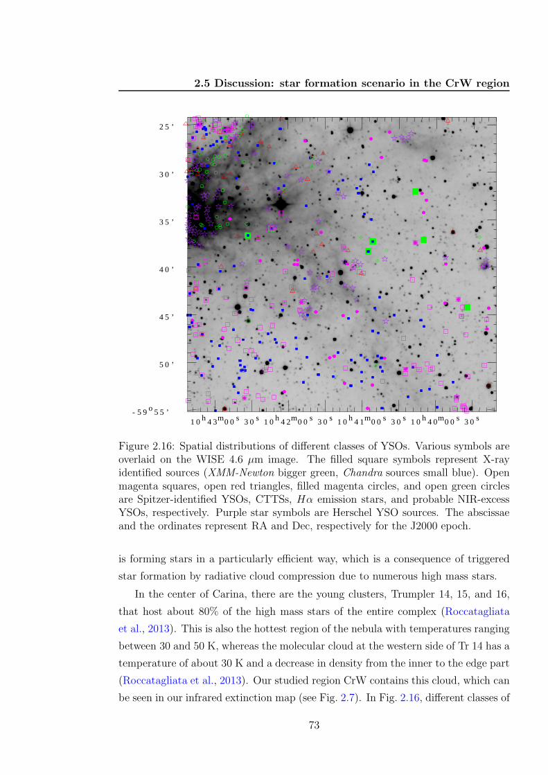
2.5 Discussion: star formation scenario in the CrW region
3 0 s1 0 4 0 0 0 h m s3 0 s1 0 4 1 0 0 h m s3 0 s1 0 4 2 0 0 h m s3 0 s1 0 4 3 0 0 h m s- 5 9 5 5 ’ o
5 0 ’
4 5 ’
4 0 ’
3 5 ’
3 0 ’
2 5 ’
Figure 2.16: Spatial distributions of different classes of YSOs. Various symbols areoverlaid on the WISE 4.6 µm image. The filled square symbols represent X-rayidentified sources (XMM-Newton bigger green, Chandra sources small blue). Openmagenta squares, open red triangles, filled magenta circles, and open green circlesare Spitzer-identified YSOs, CTTSs, Hα emission stars, and probable NIR-excessYSOs, respectively. Purple star symbols are Herschel YSO sources. The abscissaeand the ordinates represent RA and Dec, respectively for the J2000 epoch.
is forming stars in a particularly efficient way, which is a consequence of triggered
star formation by radiative cloud compression due to numerous high mass stars.
In the center of Carina, there are the young clusters, Trumpler 14, 15, and 16,
that host about 80% of the high mass stars of the entire complex (Roccatagliata
et al., 2013). This is also the hottest region of the nebula with temperatures ranging
between 30 and 50 K, whereas the molecular cloud at the western side of Tr 14 has a
temperature of about 30 K and a decrease in density from the inner to the edge part
(Roccatagliata et al., 2013). Our studied region CrW contains this cloud, which can
be seen in our infrared extinction map (see Fig. 2.7). In Fig. 2.16, different classes of
73
2. STUDY OF THE CARINA NEBULA MASSIVE STAR FORMINGREGION
YSOs identified in our study are overlaid on the WISE 4.6 µm (MIR) image. We can
easily see the extension of the dust lane in the figure from northeast to southwest of
the CrW region. The northeast region contains the outer most part of the cluster
Tr 14 along with the high density region of the molecular cloud (see Fig. 2.7). Smith
& Brooks (2008) show the spatial relationship of Tr 14, the ionized gas, the PDR
emission, the molecular gas, and the dust lane. The brightest molecular emission is
concentrated towards the dark western dust lane offset from the center of Tr 14 by
4 arcmin. The radio continuum for emission source “Car I” can also be seen here
at the interface of the dust lane and the bright Hii region. Between this source and
the molecular cloud, a widespread PDR emission can also be seen in the form of an
arc like PAH emission feature at 3.3 µm (Rathborne et al., 2002). At a projected
distance of ∼2 pc, the UV output of Tr 14 dominates the other Carina Nebula
clusters such as Tr 16 in determining the local flux at the PDR in the northern
cloud (Brooks et al., 2003; Smith, 2006a; Smith & Brooks, 2008). This spatial
sequence of Tr 14, radio source, PAH emission, and then strong molecular emission
delineates a classical edge-on PDR (Brooks et al., 2003). The edge of this region
contains many Spitzer-identified YSOs. The alignment of the YSOs in this region
may be due to the star formation triggered by high mass stars of Tr 14.
The Herschel-identified YSOs (Gaczkowski et al., 2013) are located mainly in
the high density region of the molecular clumps and in small groupings at several
places along the dust lane. Gaczkowski et al. (2013) have derived an age of ∼0.1
Myr for their sample of YSOs. The probable NIR excess stars identified in this
study also follow this region. For some of them, we derived ages .1 Myr. These
sets of identified YSOs are basically very young in nature and are embedded in the
cores of the molecular cloud. We could not say anything about the northwest region
of CrW, which is not well covered by previous surveys.
Smith et al. (2010) observed in their western mosaic (which contains most of
our observed region including the dark lane, see their Fig. 3), the YSOs density
of around 500 sources/deg2 with little signs of clustering. In this study we have
identified 467 YSOs falling in the CrW region. The overall density of this region
then turns out to be ∼1700 sources/deg2 which is higher than three times the YSOs
density given by Smith et al. (2010). Here it is worthwhile to mention that the
PCYC used in previous studies has a sensitivity problem at the ionization front
between Tr 14 and the Car I molecular cloud core to the west (Ascenso et al., 2007;
74
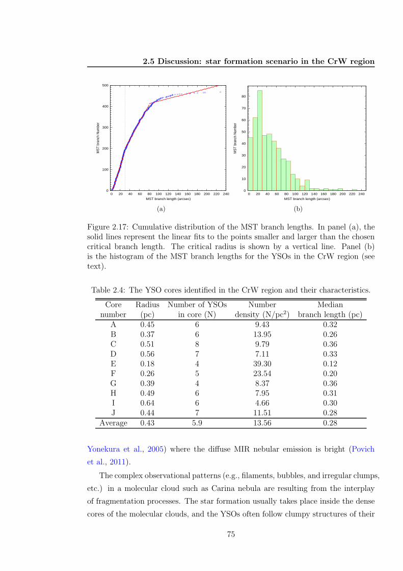
2.5 Discussion: star formation scenario in the CrW region
0
100
200
300
400
500
0 20 40 60 80 100 120 140 160 180 200 220 240
MS
T br
anch
Num
ber
MST branch length (arcsec)
(a)
0
10
20
30
40
50
60
70
80
0 20 40 60 80 100 120 140 160 180 200 220 240
MS
T br
anch
Num
ber
MST branch length (arcsec)
(b)
Figure 2.17: Cumulative distribution of the MST branch lengths. In panel (a), thesolid lines represent the linear fits to the points smaller and larger than the chosencritical branch length. The critical radius is shown by a vertical line. Panel (b)is the histogram of the MST branch lengths for the YSOs in the CrW region (seetext).
Table 2.4: The YSO cores identified in the CrW region and their characteristics.
Core Radius Number of YSOs Number Mediannumber (pc) in core (N) density (N/pc2) branch length (pc)
A 0.45 6 9.43 0.32B 0.37 6 13.95 0.26C 0.51 8 9.79 0.36D 0.56 7 7.11 0.33E 0.18 4 39.30 0.12F 0.26 5 23.54 0.20G 0.39 4 8.37 0.36H 0.49 6 7.95 0.31I 0.64 6 4.66 0.30J 0.44 7 11.51 0.28
Average 0.43 5.9 13.56 0.28
Yonekura et al., 2005) where the diffuse MIR nebular emission is bright (Povich
et al., 2011).
The complex observational patterns (e.g., filaments, bubbles, and irregular clumps,
etc.) in a molecular cloud such as Carina nebula are resulting from the interplay
of fragmentation processes. The star formation usually takes place inside the dense
cores of the molecular clouds, and the YSOs often follow clumpy structures of their
75
2. STUDY OF THE CARINA NEBULA MASSIVE STAR FORMINGREGION
parent molecular clouds (see, e.g., Allen et al., 2002; Gomez et al., 1993; Gutermuth
et al., 2005, 2008; Lada et al., 1996; Motte et al., 1998; Teixeira et al., 2006; Winston
et al., 2007). Recently, fragmentations in gas with turbulence (e.g., Ballesteros-
Paredes et al., 2007) and magnetic fields (e.g., Ward-Thompson et al., 2007) have
been discussed, leading to detailed predictions for the distributions of fragment spac-
ings. The spatial distribution of YSOs in a region can be analyzed in terms of a
typical spacing between them in order to compare this spacing to the Jeans frag-
mentation scale for a self-gravitating medium with thermal pressure (Gomez et al.,
1993). Some recent observations of star-forming regions have been analyzed in terms
of the distribution of nearest neighbor (NN) distances (see Gutermuth et al., 2005;
Teixeira et al., 2006) and find a strong peak in their histogram of NN spacings for
the protostars in young embedded clusters. This peak indicated a significant degree
of Jeans fragmentation, since this most frequent spacing agreed with an estimate
of the Jeans length for the dense gas within which the YSOs are embedded. These
results also suggest that the tendency for a narrow range of spacings among YSOs
in a cluster can last into the Class II phase of YSO evolution.
Recently, Gutermuth et al. (2009) have done a complete characterization of
the spectrum of source spacings using the minimal spanning tree (MST) of source
positions. The MST is defined as the network of lines, or branches, that connect
a set of points together such that the total length of the branches is minimized
and there are no closed loops (see, e.g., Cartwright & Whitworth, 2004; Gutermuth
et al., 2009, and references therein). Gutermuth et al. (2009) demonstrate that
the MST method yields a more complete characterization than the NN method.
Therefore, for the present study, we used the same MST algorithm to analyze the
spatial distribution of YSOs in the CrW region.
In Fig. 2.17b, we plotted the histogram of MST branch lengths for the YSOs
in the CrW region. From this plot, it is clear that they have a peak at small
spacings and that they also have a relatively long tail of large spacings. Peaked
distance distributions typically suggest a significant subregion (or subregions) of
relatively uniform, elevated surface density. By adopting an MST length threshold,
we can isolate those sources that are closer together than this threshold, yielding
populations of sources that make up a local surface density enhancement. To get this
threshold distance, in Fig. 2.17a, we plotted the cumulative distribution function
(CDF) for the branch length of YSOs. The curve shows three different slopes: first a
steep-sloped segment at short spacings then a transition segment that approximates
76
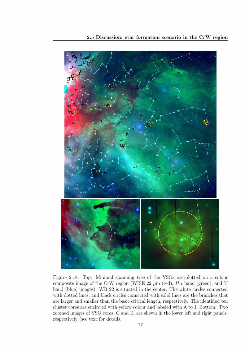
2.5 Discussion: star formation scenario in the CrW region
Figure 2.18: Top: Minimal spanning tree of the YSOs overplotted on a colourcomposite image of the CrW region (WISE 22 µm (red), Hα band (green), and Vband (blue) images). WR 22 is situated in the center. The white circles connectedwith dotted lines, and black circles connected with solid lines are the branches thatare larger and smaller than the basic critical length, respectively. The identified tencluster cores are encircled with yellow colour and labeled with A to J. Bottom: Twozoomed images of YSO cores, C and E, are shown in the lower left and right panels,respectively (see text for detail).
77
2. STUDY OF THE CARINA NEBULA MASSIVE STAR FORMINGREGION
the curved character of the intermediate-length spacings, and finally a shallow-
sloped segment at long spacings. For the present study, we have chosen the peak in
the histogram (∼30 arcsec i.e. ∼0.42 pc), which corresponds to the first steep-sloped
segment, as a threshold or critical length.
In Fig 2.18, the results from the MST analysis are overplotted on the RGB image
of the CrW region. This image was created using red, green, and blue colours for the
WISE 22 µm, Hα, and V band images, respectively. Circles and MST connections
in black deal with the objects that are more closely spaced than the critical length
(0.42 pc).
A close inspection of Fig. 2.18 reveals that the CrW region exhibits heterogeneous
structures, and there are several close concentrations of YSOs distributed along the
molecular clumps. Prominent YSO clustering can be seen in the northeastern part
of this figure and are possibly part of the star cluster Tr 14. There are also ten
cores (having MST branch lengths less than the critical distance) distributed along
the molecular cloud (indicated in Fig. 2.18). A close view of the cores C and E
can be seen in the lower left and right panels of Fig 2.18. The details about these
cores have been given in Table 2.4. The majority of the members of all these cores
are the YSOs identified in the Herschel survey having very young ages. Our result
agrees with the conclusions of Gutermuth et al. (2009) and Gunther et al. (2012),
indicating that the young protostars are found in a region having marginally higher
surface densities than the more evolved PMS stars. The average of median branch
length and core radius is found to be 0.28 pc and 0.43 pc, respectively (see Table
2.4).
To check the role of WR 22 in the formation of stars in this region, we tried to
look at the spatial distribution of YSOs (Fig. 2.19) with optical counterparts (whose
age has been derived using the V/(V −I) CMD, cf. Sect. 2.4.3.2) in the CrW region.
The general observation is that within the detection limit of optical observations, the
YSOs show mixed populations of different ages throughout the CrW region. The
extreme northeastern region contains a group of YSOs that are under the direct
influence of the high-mass stars of Tr 14, and it also shows a mixed population. For
most of the YSOs in the dust lane, we have not found their optical counterparts.
This age distribution around CrW does not show any trend even in the presence of
a very massive star such as WR 22. It seems that WR 22 has not influenced these
YSOs much. Smith et al. (2010) presented Spitzer observations of a part of the CrW
region studied here. These authors reached similar conclusions, suggesting that this
78
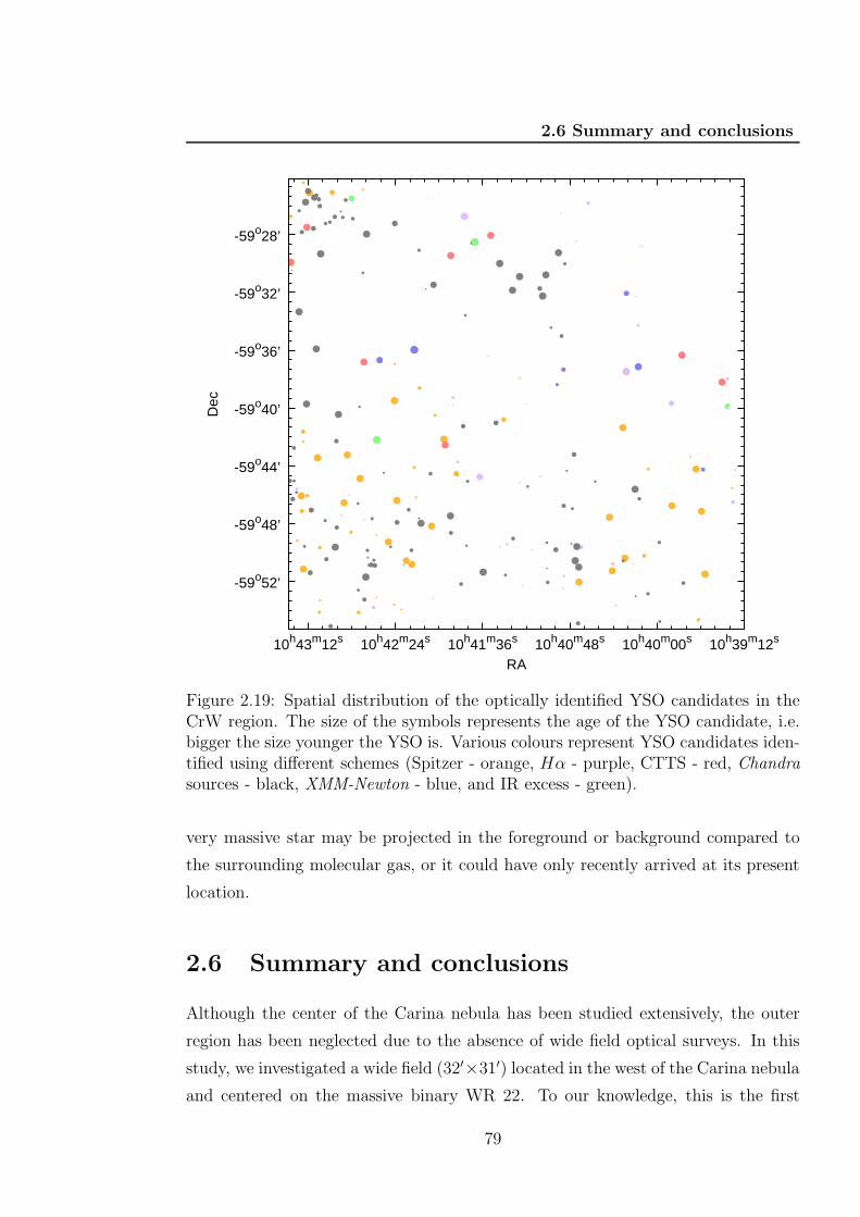
2.6 Summary and conclusions
-59o28’
-59o32’
-59o36’
-59o40’
-59o44’
-59o48’
-59o52’
10h39m12s10h40m00s10h40m48s10h41m36s10h42m24s10h43m12s
Dec
RA
Figure 2.19: Spatial distribution of the optically identified YSO candidates in theCrW region. The size of the symbols represents the age of the YSO candidate, i.e.bigger the size younger the YSO is. Various colours represent YSO candidates iden-tified using different schemes (Spitzer - orange, Hα - purple, CTTS - red, Chandrasources - black, XMM-Newton - blue, and IR excess - green).
very massive star may be projected in the foreground or background compared to
the surrounding molecular gas, or it could have only recently arrived at its present
location.
2.6 Summary and conclusions
Although the center of the Carina nebula has been studied extensively, the outer
region has been neglected due to the absence of wide field optical surveys. In this
study, we investigated a wide field (32′×31′) located in the west of the Carina nebula
and centered on the massive binary WR 22. To our knowledge, this is the first
79
2. STUDY OF THE CARINA NEBULA MASSIVE STAR FORMINGREGION
detailed study of this region. We used deep optical (UBV RI) and Hα photometric
data obtained with the WFI instrument at the ESO/MPG 2.2 m telescope (La Silla).
Our V band photometry is complete up to ∼21.5 mag. Low-resolution spectroscopy
along with Chandra, XMM-Newton, and 2MASS archival data sets, were also used
in this analysis. We generated various combinations of optical and NIR TCD, CMDs
and calculated several parameters such as reddening, reddening law, etc. We also
identified the YSOs located in the region and studied their spatial distribution using
the MST method. Ages and masses of the 241 YSOs having optical counterparts,
were derived based on V/(V − I) CMD. These YSOs have been further used to
constrain the IMF of the region. The main scientific results from our study are as
follows:
• The region shows a large amount of differential reddening with minimum and
maximum E(B − V ) values of 0.25 and 1.1 mag., respectively. This region
shows an unusual reddening law with a total-to-selective extinction ratio RV =
3.7± 0.1.
• The MK spectral types for a subsample of 15 X-ray emitting sources in the
CrW region are established that indicates that the majority of them are late
spectral type stars. There are three sources belonging to each O, A, and F
spectral types; however, six sources are of spectral type G.
• We cross-correlated the 43 XMM-Newton X-ray sources from Claeskens et al.
(2011) with our optical photometry and found that 34 of them are well matched.
Out of these 34 sources, 7 have been identified as YSOs. We also cross-
identified the Chandra X-ray sources (1465 in our region) with our source list
and found 469 objects with optical/NIR counterparts. In total, 119 X-ray
sources are identified as YSOs, four of them in common with XMM-Newton.
• We collected a sample of 467 YSOs identified in the CrW region based on
their IR-excess, Hα and X-ray emission. In some cases, the same YSOs were
identified in more than one scheme. Out of these, there are 41 Hα emitters,
105 Herschel identified YSOs, 136 Spitzer identified YSOs, and 225 2MASS
identified YSOs in our list. The YSO density for the CrW region turns out
to be ∼1700 sources/degree2, which is higher when compared to the reported
values (500 sources/degree2, Smith et al. 2010).
80
2.6 Summary and conclusions
• We calculated the age and mass of 241 individual optically identified YSOs.
Estimated ages and masses of the YSOs range from∼0.1 to 10 Myr and∼0.3 to
4.8 M⊙, respectively. This age range indicates a wide spread in the formation
of stars in the region. The majority of these YSOs are younger than 1 Myr,
and their mass is below 2 M⊙.
• We derived the IMF and calculated the slope ‘Γ’ in the CrW region. In the
mass range 0.5 < M/M⊙ < 4.8, it comes out as −1.13 ± 0.20 which is a bit
shallower than the value of −1.35 given by Salpeter (1955), and there seems
to be no break in the slope at M ∼1M⊙. The slope of the K-band luminosity
function is found to be α = 0.31± 0.01.
• The spatial distribution of all 467 YSOs has been studied in detail. The edge
of the irradiated surface between Tr 14 and the molecular cloud contains many
Spitzer identified YSOs whose formation was probably triggered by the high-
mass stars of Tr 14. The high-density region of molecular clumps contains
many probable NIR excess stars, as well as Herschel-identified YSOs that are
very young in age (.1 Myr).
• We used the well-established MST method to identify local density enhance-
ments in the YSO distributions. The northeastern part of the studied region
presents a more prominent YSO clustering. However, there are at least ten
cores of four or more very young YSO members distributed all over the CrW
region and having different core radii. The average core radii and median
branch length values for these cores are found to be 0.43 pc and 0.28 pc,
respectively. The YSOs having optical counterparts in CrW are uniformly
distributed having mixed populations of different ages. The age distribution
around CrW does not show any trend in the presence of the very massive star
WR 22. It seems that WR 22 is a foreground/background star which has not
influenced the formation of YSOs in the CrW region.
81

Chapter 3
CCSNe, progenitors: the Type IIb
supernova 2011fu
3.1 Introduction
It is commonly recognized that core-collapse supernovae (CCSNe) represent the final
stages of the life of massive stars (M > 8−10 M⊙; Anderson & James, 2009; Heger
et al., 2003a; Smartt, 2009). Generally, the fate of a massive star is governed by
its mass, metallicity, rotation and magnetic field (Fryer, 1999; Heger et al., 2003a;
Woosley & Janka, 2005). Massive stars show a wide variety in these fundamental
parameters, causing diverse observational properties among various types of CCSNe.
The presence of dominant hydrogen lines in the spectra of Type II SNe strongly
suggests that their progenitors belong to massive stars, which are still surrounded by
significantly thick hydrogen envelopes before the explosion (for a review on different
types of SNe, see Filippenko, 1997). In contrast, Type Ib events are H-deficient but
He is still present in their spectra, unlike Type Ic SNe, where both H and He features
are absent. After the discovery of SN 1987K, another class, referred as Type IIb
(see Filippenko, 1988; Woosley et al., 1987), was included in the CCSN zoo. The
observational properties of these SNe closely resemble those of Type II SNe during
the early phases, while they are more similar to Type Ib/c events at later epochs.
However, in a few cases, the spectral classification of Type IIb SNe is more
controversial: for example, SN 2000H (Benetti et al., 2000; Branch et al., 2002;
Elmhamdi et al., 2006); SN 2003bg (Filippenko & Chornock, 2003; Soderberg et al.,
2006); SN 2007Y (although this event is classified as Type Ib/c by e.g. Monard
(2007); Stritzinger et al. (2009) however, Maurer et al. (2010) suggested that it is a
83
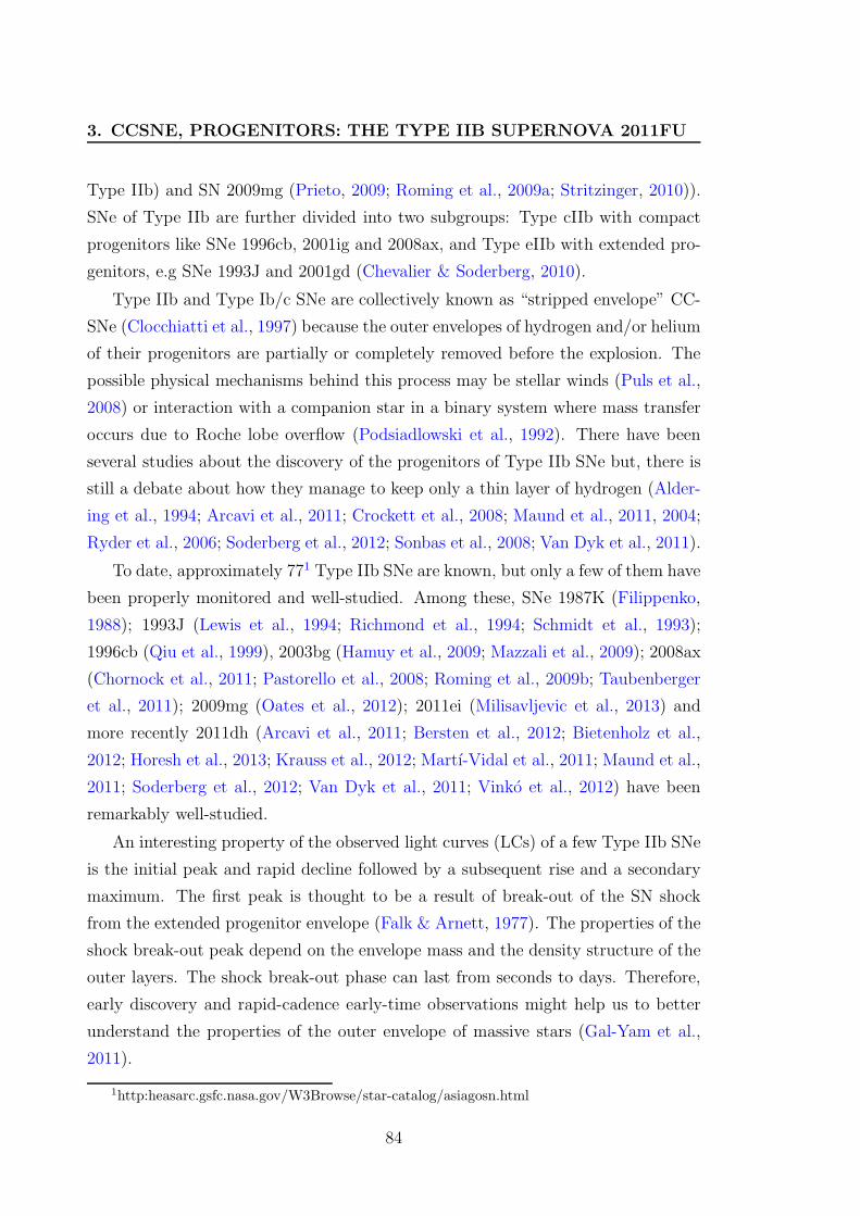
3. CCSNE, PROGENITORS: THE TYPE IIB SUPERNOVA 2011FU
Type IIb) and SN 2009mg (Prieto, 2009; Roming et al., 2009a; Stritzinger, 2010)).
SNe of Type IIb are further divided into two subgroups: Type cIIb with compact
progenitors like SNe 1996cb, 2001ig and 2008ax, and Type eIIb with extended pro-
genitors, e.g SNe 1993J and 2001gd (Chevalier & Soderberg, 2010).
Type IIb and Type Ib/c SNe are collectively known as “stripped envelope” CC-
SNe (Clocchiatti et al., 1997) because the outer envelopes of hydrogen and/or helium
of their progenitors are partially or completely removed before the explosion. The
possible physical mechanisms behind this process may be stellar winds (Puls et al.,
2008) or interaction with a companion star in a binary system where mass transfer
occurs due to Roche lobe overflow (Podsiadlowski et al., 1992). There have been
several studies about the discovery of the progenitors of Type IIb SNe but, there is
still a debate about how they manage to keep only a thin layer of hydrogen (Alder-
ing et al., 1994; Arcavi et al., 2011; Crockett et al., 2008; Maund et al., 2011, 2004;
Ryder et al., 2006; Soderberg et al., 2012; Sonbas et al., 2008; Van Dyk et al., 2011).
To date, approximately 771 Type IIb SNe are known, but only a few of them have
been properly monitored and well-studied. Among these, SNe 1987K (Filippenko,
1988); 1993J (Lewis et al., 1994; Richmond et al., 1994; Schmidt et al., 1993);
1996cb (Qiu et al., 1999), 2003bg (Hamuy et al., 2009; Mazzali et al., 2009); 2008ax
(Chornock et al., 2011; Pastorello et al., 2008; Roming et al., 2009b; Taubenberger
et al., 2011); 2009mg (Oates et al., 2012); 2011ei (Milisavljevic et al., 2013) and
more recently 2011dh (Arcavi et al., 2011; Bersten et al., 2012; Bietenholz et al.,
2012; Horesh et al., 2013; Krauss et al., 2012; Martı-Vidal et al., 2011; Maund et al.,
2011; Soderberg et al., 2012; Van Dyk et al., 2011; Vinko et al., 2012) have been
remarkably well-studied.
An interesting property of the observed light curves (LCs) of a few Type IIb SNe
is the initial peak and rapid decline followed by a subsequent rise and a secondary
maximum. The first peak is thought to be a result of break-out of the SN shock
from the extended progenitor envelope (Falk & Arnett, 1977). The properties of the
shock break-out peak depend on the envelope mass and the density structure of the
outer layers. The shock break-out phase can last from seconds to days. Therefore,
early discovery and rapid-cadence early-time observations might help us to better
understand the properties of the outer envelope of massive stars (Gal-Yam et al.,
2011).
1http:heasarc.gsfc.nasa.gov/W3Browse/star-catalog/asiagosn.html
84
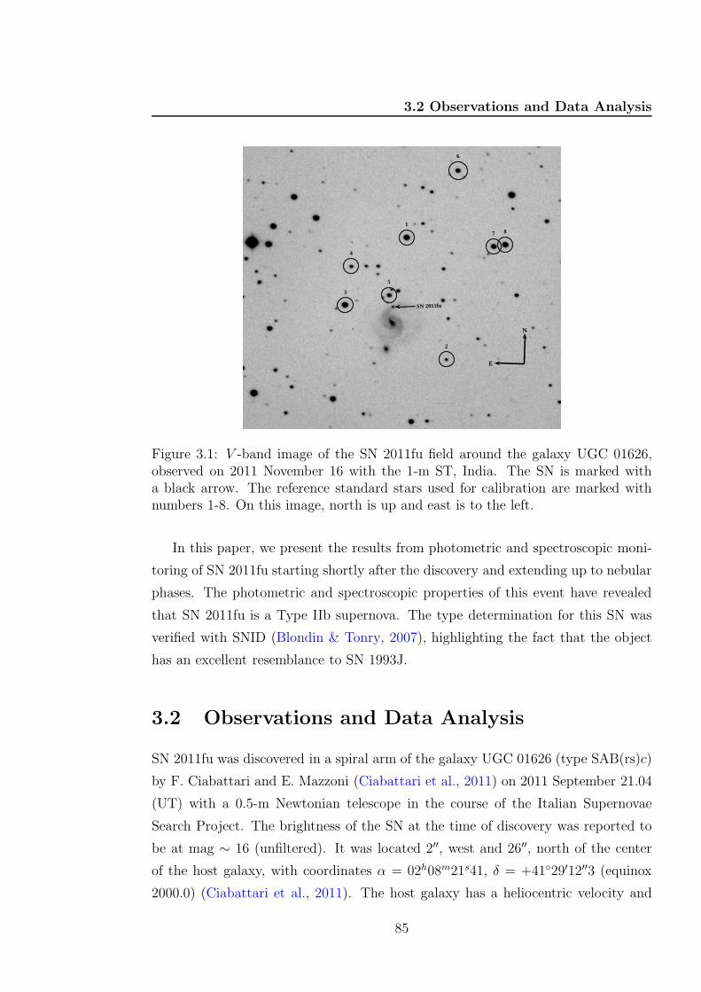
3.2 Observations and Data Analysis
E
N
6
SN 2011fu
87
5
4
3
2
1
Figure 3.1: V -band image of the SN 2011fu field around the galaxy UGC 01626,observed on 2011 November 16 with the 1-m ST, India. The SN is marked witha black arrow. The reference standard stars used for calibration are marked withnumbers 1-8. On this image, north is up and east is to the left.
In this paper, we present the results from photometric and spectroscopic moni-
toring of SN 2011fu starting shortly after the discovery and extending up to nebular
phases. The photometric and spectroscopic properties of this event have revealed
that SN 2011fu is a Type IIb supernova. The type determination for this SN was
verified with SNID (Blondin & Tonry, 2007), highlighting the fact that the object
has an excellent resemblance to SN 1993J.
3.2 Observations and Data Analysis
SN 2011fu was discovered in a spiral arm of the galaxy UGC 01626 (type SAB(rs)c)
by F. Ciabattari and E. Mazzoni (Ciabattari et al., 2011) on 2011 September 21.04
(UT) with a 0.5-m Newtonian telescope in the course of the Italian Supernovae
Search Project. The brightness of the SN at the time of discovery was reported to
be at mag ∼ 16 (unfiltered). It was located 2′′, west and 26′′, north of the center
of the host galaxy, with coordinates α = 02h08m21s41, δ = +4129′12′′3 (equinox
2000.0) (Ciabattari et al., 2011). The host galaxy has a heliocentric velocity and
85
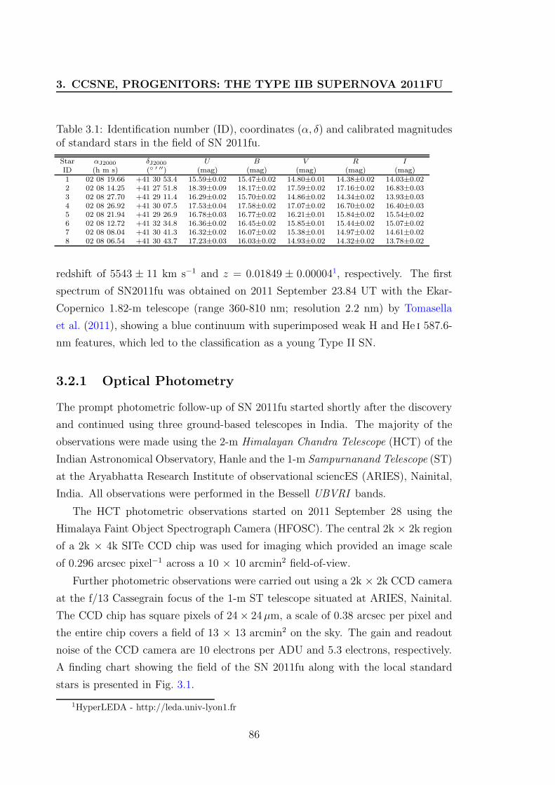
3. CCSNE, PROGENITORS: THE TYPE IIB SUPERNOVA 2011FU
Table 3.1: Identification number (ID), coordinates (α, δ) and calibrated magnitudesof standard stars in the field of SN 2011fu.
Star αJ2000 δJ2000 U B V R I
ID (h m s) ( ′ ′′) (mag) (mag) (mag) (mag) (mag)1 02 08 19.66 +41 30 53.4 15.59±0.02 15.47±0.02 14.80±0.01 14.38±0.02 14.03±0.022 02 08 14.25 +41 27 51.8 18.39±0.09 18.17±0.02 17.59±0.02 17.16±0.02 16.83±0.033 02 08 27.70 +41 29 11.4 16.29±0.02 15.70±0.02 14.86±0.02 14.34±0.02 13.93±0.034 02 08 26.92 +41 30 07.5 17.53±0.04 17.58±0.02 17.07±0.02 16.70±0.02 16.40±0.035 02 08 21.94 +41 29 26.9 16.78±0.03 16.77±0.02 16.21±0.01 15.84±0.02 15.54±0.026 02 08 12.72 +41 32 34.8 16.36±0.02 16.45±0.02 15.85±0.01 15.44±0.02 15.07±0.027 02 08 08.04 +41 30 41.3 16.32±0.02 16.07±0.02 15.38±0.01 14.97±0.02 14.61±0.028 02 08 06.54 +41 30 43.7 17.23±0.03 16.03±0.02 14.93±0.02 14.32±0.02 13.78±0.02
redshift of 5543 ± 11 km s−1 and z = 0.01849 ± 0.000041, respectively. The first
spectrum of SN2011fu was obtained on 2011 September 23.84 UT with the Ekar-
Copernico 1.82-m telescope (range 360-810 nm; resolution 2.2 nm) by Tomasella
et al. (2011), showing a blue continuum with superimposed weak H and He i 587.6-
nm features, which led to the classification as a young Type II SN.
3.2.1 Optical Photometry
The prompt photometric follow-up of SN 2011fu started shortly after the discovery
and continued using three ground-based telescopes in India. The majority of the
observations were made using the 2-m Himalayan Chandra Telescope (HCT) of the
Indian Astronomical Observatory, Hanle and the 1-m Sampurnanand Telescope (ST)
at the Aryabhatta Research Institute of observational sciencES (ARIES), Nainital,
India. All observations were performed in the Bessell UBVRI bands.
The HCT photometric observations started on 2011 September 28 using the
Himalaya Faint Object Spectrograph Camera (HFOSC). The central 2k × 2k region
of a 2k × 4k SITe CCD chip was used for imaging which provided an image scale
of 0.296 arcsec pixel−1 across a 10 × 10 arcmin2 field-of-view.
Further photometric observations were carried out using a 2k × 2k CCD camera
at the f/13 Cassegrain focus of the 1-m ST telescope situated at ARIES, Nainital.
The CCD chip has square pixels of 24× 24µm, a scale of 0.38 arcsec per pixel and
the entire chip covers a field of 13 × 13 arcmin2 on the sky. The gain and readout
noise of the CCD camera are 10 electrons per ADU and 5.3 electrons, respectively.
A finding chart showing the field of the SN 2011fu along with the local standard
stars is presented in Fig. 3.1.
1HyperLEDA - http://leda.univ-lyon1.fr
86
3.2 Observations and Data Analysis
In addition, we also observed this SN in the V and R bands on 2011 December
01 and 2012 March 02 using the 1.3m Devasthal Fast Optical Telescope (DFOT)
(Sagar et al., 2012, 2011), recently installed at Devasthal, Naintial. DFOT uses a
2048 × 2048 ANDOR CCD camera having 13.5µm× 13.5µm pixels mounted at the
f/4 Cassegrain focus of the telescope. With a 0.54 arcsec per pixel plate scale, the
entire chip covers a 18 × 18 arcmin2 field-of-view on the sky. The CCD can be read
out with 31, 62, 500 and 1000 kHz speed, with a system RMS noise of 2.5, 4.1, 6.5,
7 electrons and a gain of 0.7, 1.4, 2, 2 electrons/ADU respectively. We selected the
500 kHz readout frequency during our observations.
To improve the signal-to-noise ratio (S/N), all the photometric observations
were carried out with a 2×2 binning. Along with the science frames several bias
and twilight flat frames were also collected. Alignment and determination of the
mean FWHM on all science frames were performed after the usual bias subtraction,
flat fielding and cosmic-ray removal. The standard tasks available in iraf and
daophot (Stetson, 1987, 1992) were used for pre-processing and photometry.
The pre-processing steps for images taken with all three telescopes were per-
formed in a similar fashion. The stellar FWHM on the V -band frames typically
varied from 2′′, to 4′′, with a median value of around 2′′5. We also co-added indi-
vidual frames, wherever necessary, before computing the final photometry.
For photometric calibration, we observed the standard field PG0231 (Landolt,
2009) in UBVRI bands with the 1-m ST on 2011 December 17 under good pho-
tometric conditions (transparent sky, seeing FWHM in V ∼ 2′′). The profile fit-
ting technique was applied for the photometry of SN 2011fu and Landolt field and
then instrumental magnitudes were converted into standard system following least-
square linear regression procedures outlined in Stetson (1992). The average atmo-
spheric extinction values (0.57, 0.28, 0.17, 0.11 and 0.07 mag per unit airmass for
U , B, V , R and I bands, respectively) for the site were adopted from Kumar et al.
(2000). The chosen Landolt stars for calibration were in the brightness range of
12.77 ≤ V ≤ 16.11 mag and colour range of −0.33 ≤ B − V ≤ 1.45 mag. Us-
ing these stars, transformation to the standard system was derived by applying the
following zero-points and colour coefficients:
u− U = (7.27± 0.01) + (−0.08± 0.02)(U −B)
b− B = (4.90± 0.004) + (−0.04± 0.01)(B − V )
v − V = (4.34± 0.01) + (−0.04± 0.01)(B − V )
87
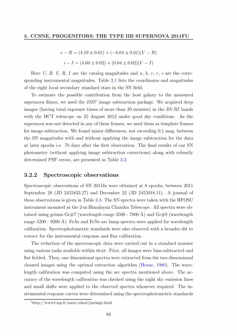
3. CCSNE, PROGENITORS: THE TYPE IIB SUPERNOVA 2011FU
r − R = (4.19± 0.01) + (−0.04± 0.01)(V − R)
i− I = (4.60± 0.02) + (0.04± 0.02)(V − I)
Here U, B, V, R, I are the catalog magnitudes and u, b, v, r, i are the corre-
sponding instrumental magnitudes. Table 3.1 lists the coordinates and magnitudes
of the eight local secondary standard stars in the SN field.
To estimate the possible contribution from the host galaxy to the measured
supernova fluxes, we used the ISIS1 image subtraction package. We acquired deep
images (having total exposure times of more than 20 minutes) in the BV RI bands
with the HCT telescope on 25 August 2012 under good sky conditions. As the
supernova was not detected in any of these frames, we used them as template frames
for image subtraction. We found minor differences, not exceeding 0.1 mag, between
the SN magnitudes with and without applying the image subtraction for the data
at later epochs i.e. 70 days after the first observation. The final results of our SN
photometry (without applying image subtraction corrections) along with robustly
determined PSF errors, are presented in Table 3.2.
3.2.2 Spectroscopic observations
Spectroscopic observations of SN 2011fu were obtained at 8 epochs, between 2011
September 28 (JD 2455833.27) and December 22 (JD 2455918.11). A journal of
these observations is given in Table 3.3. The SN spectra were taken with the HFOSC
instrument mounted at the 2-m Himalayan Chandra Telescope. All spectra were ob-
tained using grisms Gr#7 (wavelength range 3500 - 7800 A) and Gr#8 (wavelength
range 5200 - 9200 A). FeAr and FeNe arc lamp spectra were applied for wavelength
calibration. Spectrophotometric standards were also observed with a broader slit to
correct for the instrumental response and flux calibration.
The reduction of the spectroscopic data were carried out in a standard manner
using various tasks available within iraf. First, all images were bias-subtracted and
flat fielded. Then, one dimensional spectra were extracted from the two-dimensional
cleaned images using the optimal extraction algorithm (Horne, 1986). The wave-
length calibration was computed using the arc spectra mentioned above. The ac-
curacy of the wavelength calibration was checked using the night sky emission lines
and small shifts were applied to the observed spectra whenever required. The in-
strumental response curves were determined using the spectrophotometric standards
1http://www2.iap.fr/users/alard/package.html
88
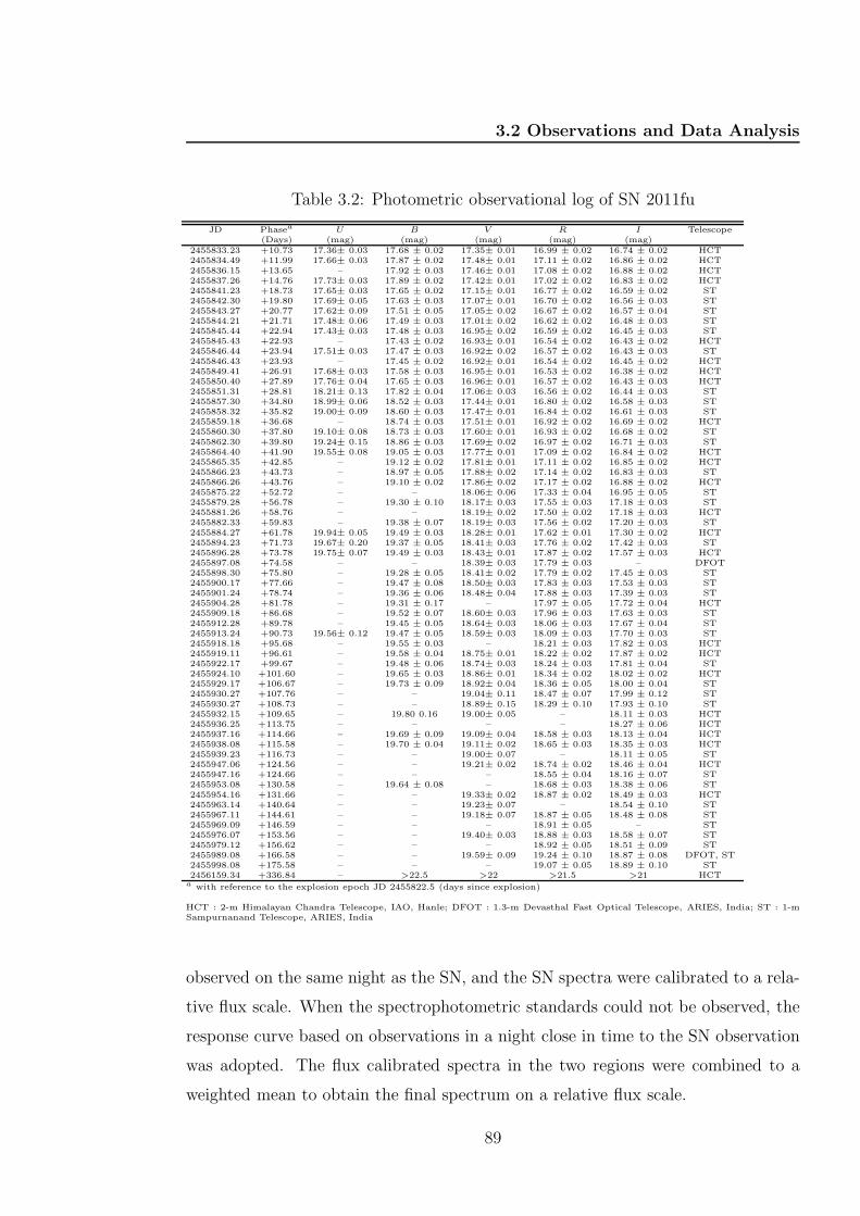
3.2 Observations and Data Analysis
Table 3.2: Photometric observational log of SN 2011fu
JD Phasea U B V R I Telescope(Days) (mag) (mag) (mag) (mag) (mag)
2455833.23 +10.73 17.36± 0.03 17.68 ± 0.02 17.35± 0.01 16.99 ± 0.02 16.74 ± 0.02 HCT2455834.49 +11.99 17.66± 0.03 17.87 ± 0.02 17.48± 0.01 17.11 ± 0.02 16.86 ± 0.02 HCT2455836.15 +13.65 – 17.92 ± 0.03 17.46± 0.01 17.08 ± 0.02 16.88 ± 0.02 HCT2455837.26 +14.76 17.73± 0.03 17.89 ± 0.02 17.42± 0.01 17.02 ± 0.02 16.83 ± 0.02 HCT2455841.23 +18.73 17.65± 0.03 17.65 ± 0.02 17.15± 0.01 16.77 ± 0.02 16.59 ± 0.02 ST2455842.30 +19.80 17.69± 0.05 17.63 ± 0.03 17.07± 0.01 16.70 ± 0.02 16.56 ± 0.03 ST2455843.27 +20.77 17.62± 0.09 17.51 ± 0.05 17.05± 0.02 16.67 ± 0.02 16.57 ± 0.04 ST2455844.21 +21.71 17.48± 0.06 17.49 ± 0.03 17.01± 0.02 16.62 ± 0.02 16.48 ± 0.03 ST2455845.44 +22.94 17.43± 0.03 17.48 ± 0.03 16.95± 0.02 16.59 ± 0.02 16.45 ± 0.03 ST2455845.43 +22.93 – 17.43 ± 0.02 16.93± 0.01 16.54 ± 0.02 16.43 ± 0.02 HCT2455846.44 +23.94 17.51± 0.03 17.47 ± 0.03 16.92± 0.02 16.57 ± 0.02 16.43 ± 0.03 ST2455846.43 +23.93 – 17.45 ± 0.02 16.92± 0.01 16.54 ± 0.02 16.45 ± 0.02 HCT2455849.41 +26.91 17.68± 0.03 17.58 ± 0.03 16.95± 0.01 16.53 ± 0.02 16.38 ± 0.02 HCT2455850.40 +27.89 17.76± 0.04 17.65 ± 0.03 16.96± 0.01 16.57 ± 0.02 16.43 ± 0.03 HCT2455851.31 +28.81 18.21± 0.13 17.82 ± 0.04 17.06± 0.03 16.56 ± 0.02 16.44 ± 0.03 ST2455857.30 +34.80 18.99± 0.06 18.52 ± 0.03 17.44± 0.01 16.80 ± 0.02 16.58 ± 0.03 ST2455858.32 +35.82 19.00± 0.09 18.60 ± 0.03 17.47± 0.01 16.84 ± 0.02 16.61 ± 0.03 ST2455859.18 +36.68 – 18.74 ± 0.03 17.51± 0.01 16.92 ± 0.02 16.69 ± 0.02 HCT2455860.30 +37.80 19.10± 0.08 18.73 ± 0.03 17.60± 0.01 16.93 ± 0.02 16.68 ± 0.02 ST2455862.30 +39.80 19.24± 0.15 18.86 ± 0.03 17.69± 0.02 16.97 ± 0.02 16.71 ± 0.03 ST2455864.40 +41.90 19.55± 0.08 19.05 ± 0.03 17.77± 0.01 17.09 ± 0.02 16.84 ± 0.02 HCT2455865.35 +42.85 – 19.12 ± 0.02 17.81± 0.01 17.11 ± 0.02 16.85 ± 0.02 HCT2455866.23 +43.73 – 18.97 ± 0.05 17.88± 0.02 17.14 ± 0.02 16.83 ± 0.03 ST2455866.26 +43.76 – 19.10 ± 0.02 17.86± 0.02 17.17 ± 0.02 16.88 ± 0.02 HCT2455875.22 +52.72 – – 18.06± 0.06 17.33 ± 0.04 16.95 ± 0.05 ST2455879.28 +56.78 – 19.30 ± 0.10 18.17± 0.03 17.55 ± 0.03 17.18 ± 0.03 ST2455881.26 +58.76 – – 18.19± 0.02 17.50 ± 0.02 17.18 ± 0.03 HCT2455882.33 +59.83 – 19.38 ± 0.07 18.19± 0.03 17.56 ± 0.02 17.20 ± 0.03 ST2455884.27 +61.78 19.94± 0.05 19.49 ± 0.03 18.28± 0.01 17.62 ± 0.01 17.30 ± 0.02 HCT2455894.23 +71.73 19.67± 0.20 19.37 ± 0.05 18.41± 0.03 17.76 ± 0.02 17.42 ± 0.03 ST2455896.28 +73.78 19.75± 0.07 19.49 ± 0.03 18.43± 0.01 17.87 ± 0.02 17.57 ± 0.03 HCT2455897.08 +74.58 – – 18.39± 0.03 17.79 ± 0.03 – DFOT2455898.30 +75.80 – 19.28 ± 0.05 18.41± 0.02 17.79 ± 0.02 17.45 ± 0.03 ST2455900.17 +77.66 – 19.47 ± 0.08 18.50± 0.03 17.83 ± 0.03 17.53 ± 0.03 ST2455901.24 +78.74 – 19.36 ± 0.06 18.48± 0.04 17.88 ± 0.03 17.39 ± 0.03 ST2455904.28 +81.78 – 19.31 ± 0.17 – 17.97 ± 0.05 17.72 ± 0.04 HCT2455909.18 +86.68 – 19.52 ± 0.07 18.60± 0.03 17.96 ± 0.03 17.63 ± 0.03 ST2455912.28 +89.78 – 19.45 ± 0.05 18.64± 0.03 18.06 ± 0.03 17.67 ± 0.04 ST2455913.24 +90.73 19.56± 0.12 19.47 ± 0.05 18.59± 0.03 18.09 ± 0.03 17.70 ± 0.03 ST2455918.18 +95.68 – 19.55 ± 0.03 – 18.21 ± 0.03 17.82 ± 0.03 HCT2455919.11 +96.61 – 19.58 ± 0.04 18.75± 0.01 18.22 ± 0.02 17.87 ± 0.02 HCT2455922.17 +99.67 – 19.48 ± 0.06 18.74± 0.03 18.24 ± 0.03 17.81 ± 0.04 ST2455924.10 +101.60 – 19.65 ± 0.03 18.86± 0.01 18.34 ± 0.02 18.02 ± 0.02 HCT2455929.17 +106.67 – 19.73 ± 0.09 18.92± 0.04 18.36 ± 0.05 18.00 ± 0.04 ST2455930.27 +107.76 – – 19.04± 0.11 18.47 ± 0.07 17.99 ± 0.12 ST2455930.27 +108.73 – – 18.89± 0.15 18.29 ± 0.10 17.93 ± 0.10 ST2455932.15 +109.65 – 19.80 0.16 19.00± 0.05 – 18.11 ± 0.03 HCT2455936.25 +113.75 – – – – 18.27 ± 0.06 HCT2455937.16 +114.66 – 19.69 ± 0.09 19.09± 0.04 18.58 ± 0.03 18.13 ± 0.04 HCT2455938.08 +115.58 – 19.70 ± 0.04 19.11± 0.02 18.65 ± 0.03 18.35 ± 0.03 HCT2455939.23 +116.73 – – 19.00± 0.07 – 18.11 ± 0.05 ST2455947.06 +124.56 – – 19.21± 0.02 18.74 ± 0.02 18.46 ± 0.04 HCT2455947.16 +124.66 – – – 18.55 ± 0.04 18.16 ± 0.07 ST2455953.08 +130.58 – 19.64 ± 0.08 – 18.68 ± 0.03 18.38 ± 0.06 ST2455954.16 +131.66 – – 19.33± 0.02 18.87 ± 0.02 18.49 ± 0.03 HCT2455963.14 +140.64 – – 19.23± 0.07 – 18.54 ± 0.10 ST2455967.11 +144.61 – – 19.18± 0.07 18.87 ± 0.05 18.48 ± 0.08 ST2455969.09 +146.59 – – – 18.91 ± 0.05 – ST2455976.07 +153.56 – – 19.40± 0.03 18.88 ± 0.03 18.58 ± 0.07 ST2455979.12 +156.62 – – – 18.92 ± 0.05 18.51 ± 0.09 ST2455989.08 +166.58 – – 19.59± 0.09 19.24 ± 0.10 18.87 ± 0.08 DFOT, ST2455998.08 +175.58 – – – 19.07 ± 0.05 18.89 ± 0.10 ST2456159.34 +336.84 – >22.5 >22 >21.5 >21 HCT
a with reference to the explosion epoch JD 2455822.5 (days since explosion)
HCT : 2-m Himalayan Chandra Telescope, IAO, Hanle; DFOT : 1.3-m Devasthal Fast Optical Telescope, ARIES, India; ST : 1-mSampurnanand Telescope, ARIES, India
observed on the same night as the SN, and the SN spectra were calibrated to a rela-
tive flux scale. When the spectrophotometric standards could not be observed, the
response curve based on observations in a night close in time to the SN observation
was adopted. The flux calibrated spectra in the two regions were combined to a
weighted mean to obtain the final spectrum on a relative flux scale.
89
3. CCSNE, PROGENITORS: THE TYPE IIB SUPERNOVA 2011FU
Figure 3.2: Observed UBVRI light curves of SN 2011fu. For clarity, the light curvesin different bands have been shifted vertically by the values indicated in the legend.Black solid lines represent the light curves of SN 1993J (Lewis et al., 1994) over-plotted with appropriate shifts. The explosion date of SN 2011fu was taken to be2011 September 18± 2, as described in Sect. 3.3.1.
Finally, the spectra were brought to an absolute flux scale using zero points
determined from the calibrated, broad-band UBVRI magnitudes. The SN spectra
were also corrected for the redshift of the host galaxy (z = 0.018), and de-reddened
assuming a total reddening of E(B − V ) = 0.22 mag (see Sect. 3.3.3). The telluric
lines have not been removed from the spectra.
90
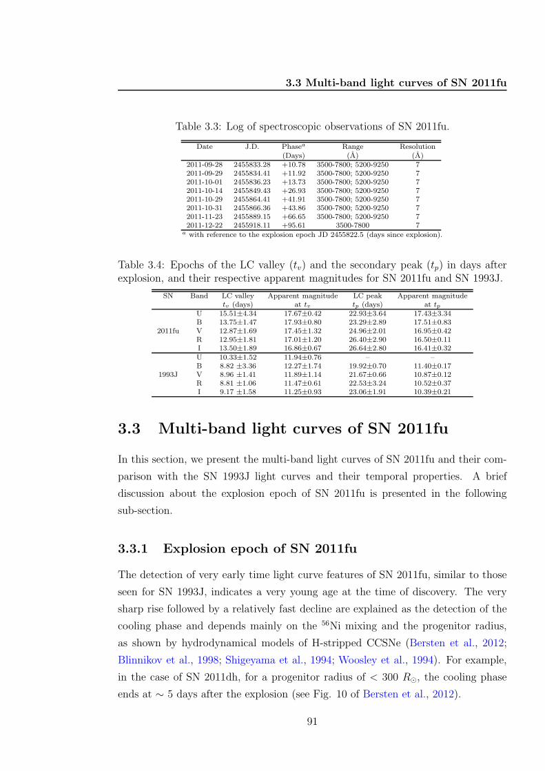
3.3 Multi-band light curves of SN 2011fu
Table 3.3: Log of spectroscopic observations of SN 2011fu.
Date J.D. Phasea Range Resolution(Days) (A) (A)
2011-09-28 2455833.28 +10.78 3500-7800; 5200-9250 72011-09-29 2455834.41 +11.92 3500-7800; 5200-9250 72011-10-01 2455836.23 +13.73 3500-7800; 5200-9250 72011-10-14 2455849.43 +26.93 3500-7800; 5200-9250 72011-10-29 2455864.41 +41.91 3500-7800; 5200-9250 72011-10-31 2455866.36 +43.86 3500-7800; 5200-9250 72011-11-23 2455889.15 +66.65 3500-7800; 5200-9250 72011-12-22 2455918.11 +95.61 3500-7800 7
a with reference to the explosion epoch JD 2455822.5 (days since explosion).
Table 3.4: Epochs of the LC valley (tv) and the secondary peak (tp) in days afterexplosion, and their respective apparent magnitudes for SN 2011fu and SN 1993J.
SN Band LC valley Apparent magnitude LC peak Apparent magnitudetv (days) at tv tp (days) at tp
U 15.51±4.34 17.67±0.42 22.93±3.64 17.43±3.34B 13.75±1.47 17.93±0.80 23.29±2.89 17.51±0.83
2011fu V 12.87±1.69 17.45±1.32 24.96±2.01 16.95±0.42R 12.95±1.81 17.01±1.20 26.40±2.90 16.50±0.11I 13.50±1.89 16.86±0.67 26.64±2.80 16.41±0.32U 10.33±1.52 11.94±0.76 – –B 8.82 ±3.36 12.27±1.74 19.92±0.70 11.40±0.17
1993J V 8.96 ±1.41 11.89±1.14 21.67±0.66 10.87±0.12R 8.81 ±1.06 11.47±0.61 22.53±3.24 10.52±0.37I 9.17 ±1.58 11.25±0.93 23.06±1.91 10.39±0.21
3.3 Multi-band light curves of SN 2011fu
In this section, we present the multi-band light curves of SN 2011fu and their com-
parison with the SN 1993J light curves and their temporal properties. A brief
discussion about the explosion epoch of SN 2011fu is presented in the following
sub-section.
3.3.1 Explosion epoch of SN 2011fu
The detection of very early time light curve features of SN 2011fu, similar to those
seen for SN 1993J, indicates a very young age at the time of discovery. The very
sharp rise followed by a relatively fast decline are explained as the detection of the
cooling phase and depends mainly on the 56Ni mixing and the progenitor radius,
as shown by hydrodynamical models of H-stripped CCSNe (Bersten et al., 2012;
Blinnikov et al., 1998; Shigeyama et al., 1994; Woosley et al., 1994). For example,
in the case of SN 2011dh, for a progenitor radius of < 300 R⊙, the cooling phase
ends at ∼ 5 days after the explosion (see Fig. 10 of Bersten et al., 2012).
91
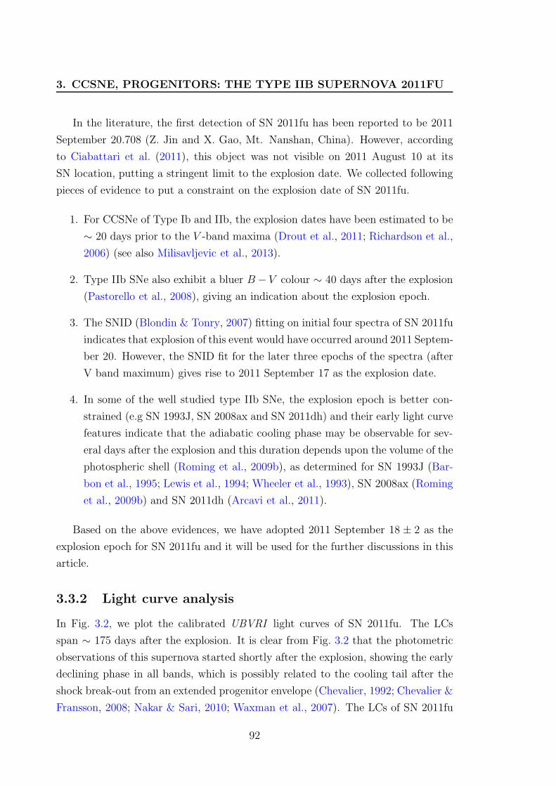
3. CCSNE, PROGENITORS: THE TYPE IIB SUPERNOVA 2011FU
In the literature, the first detection of SN 2011fu has been reported to be 2011
September 20.708 (Z. Jin and X. Gao, Mt. Nanshan, China). However, according
to Ciabattari et al. (2011), this object was not visible on 2011 August 10 at its
SN location, putting a stringent limit to the explosion date. We collected following
pieces of evidence to put a constraint on the explosion date of SN 2011fu.
1. For CCSNe of Type Ib and IIb, the explosion dates have been estimated to be
∼ 20 days prior to the V -band maxima (Drout et al., 2011; Richardson et al.,
2006) (see also Milisavljevic et al., 2013).
2. Type IIb SNe also exhibit a bluer B− V colour ∼ 40 days after the explosion
(Pastorello et al., 2008), giving an indication about the explosion epoch.
3. The SNID (Blondin & Tonry, 2007) fitting on initial four spectra of SN 2011fu
indicates that explosion of this event would have occurred around 2011 Septem-
ber 20. However, the SNID fit for the later three epochs of the spectra (after
V band maximum) gives rise to 2011 September 17 as the explosion date.
4. In some of the well studied type IIb SNe, the explosion epoch is better con-
strained (e.g SN 1993J, SN 2008ax and SN 2011dh) and their early light curve
features indicate that the adiabatic cooling phase may be observable for sev-
eral days after the explosion and this duration depends upon the volume of the
photospheric shell (Roming et al., 2009b), as determined for SN 1993J (Bar-
bon et al., 1995; Lewis et al., 1994; Wheeler et al., 1993), SN 2008ax (Roming
et al., 2009b) and SN 2011dh (Arcavi et al., 2011).
Based on the above evidences, we have adopted 2011 September 18 ± 2 as the
explosion epoch for SN 2011fu and it will be used for the further discussions in this
article.
3.3.2 Light curve analysis
In Fig. 3.2, we plot the calibrated UBVRI light curves of SN 2011fu. The LCs
span ∼ 175 days after the explosion. It is clear from Fig. 3.2 that the photometric
observations of this supernova started shortly after the explosion, showing the early
declining phase in all bands, which is possibly related to the cooling tail after the
shock break-out from an extended progenitor envelope (Chevalier, 1992; Chevalier &
Fransson, 2008; Nakar & Sari, 2010; Waxman et al., 2007). The LCs of SN 2011fu
92
3.3 Multi-band light curves of SN 2011fu
are strikingly similar to those of SN 1993J, both in the initial and the following
phases, exhibiting valley-like structures followed by rising peaks in all bands. At
late epochs the LCs are monotonically decreasing in all bands, as expected for
expanding, cooling ejecta heated by only the radioactive decay of 56Ni and 56Co.
Beside SNe 1993J and 2011dh, SN 2011fu is the third known case among IIb SNe
to date where all the initial decline phase, the rise of the broader secondary peak
and the final decline have been observed (although Roming et al. (2010) reported
similar observations for SN 2008ax). In the following, we refer the first minimum
of the LC (when the initial decline stops and the rise to the secondary maximum
starts) as the “valley”.
To determine the epochs of the valleys (tv, in days), the subsequent peaks (tp, in
days) and their corresponding brightness values, we fitted a third-order polynomial
using a χ2 minimization technique to the LCs of both SN 2011fu and SN 1993J.
The errors in the fitting procedure were estimated by the error propagation method.
We have taken 1993 March 27.5 as the explosion date for SN 1993J (Wheeler et al.,
1993). The derived values of tv, tp and corresponding brightness values for both
SNe are listed in Table 3.4.
The values of tv and tp for both these SNe are similar within the errors in all the
bands. However, for both SNe, the light curves peak earlier in the blue bands than
in the red bands (see Table 3.4) which is a common feature seen in CCSNe. By
applying the linear regression method, the decline and rising rates (in mag day−1)
were also estimated for the three phases, i.e. the pre-valley (α1), valley-to-peak (α2)
and after-peak phases (α3). The results of the fitting are shown in Table 3.5. These
values suggest that for SN 2011fu the pre-valley decay rates (α1) are steeper (i.e.
the decay is faster) at shorter wavelengths. This is also true for SN 1993J, where
the decay rates (α1) were even steeper. Thus, the initial LC decay of SN 1993J was
steeper than that of SN 2011fu during this early phase (see also Barbon et al., 1995).
Between valley to peak phase (α2), the LC of SN 2011fu evolved with a similar rate
in all the bands, but slower than that seen for SN 1993J. During the post-peak
phase, the LCs gradually became flatter at longer wavelengths (see the α3 values in
Table 3.5). This trend has also been observed for SN 1993J and other Type IIb SNe.
The B-band LC of SN 2011fu between 50 and 100 days after explosion might even
show a plateau, similar to SNe 1993J (see Fig. 3 of Lewis et al., 1994) and 1996cb
(see Fig. 2 and the discussions of Qiu et al., 1999). The plateau-like behaviour of
the U -band LC of SN 2011fu is more prominent than the U -band LC of SN 1993J.
93
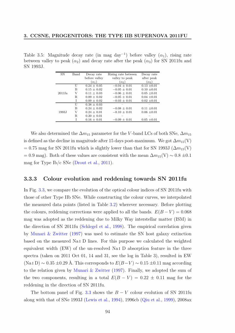
3. CCSNE, PROGENITORS: THE TYPE IIB SUPERNOVA 2011FU
Table 3.5: Magnitude decay rate (in mag day−1) before valley (α1), rising ratebetween valley to peak (α2) and decay rate after the peak (α3) for SN 2011fu andSN 1993J.
SN Band Decay rate Rising rate between Decay ratebefore valley valley to peak after peak
(α1) (α2) (α3)U 0.24 ± 0.05 −0.04 ± 0.01 0.13 ±0.01B 0.15 ± 0.02 −0.05 ± 0.01 0.10 ±0.01
2011fu V 0.11 ± 0.03 −0.06 ± 0.01 0.05 ±0.01R 0.09 ± 0.02 −0.05 ± 0.01 0.04 ±0.01I 0.09 ± 0.02 −0.03 ± 0.01 0.02 ±0.01U 0.38 ± 0.03 – –B 0.24 ± 0.02 −0.08 ± 0.01 0.11 ±0.01
1993J V 0.24 ± 0.01 −0.10 ± 0.01 0.06 ±0.01R 0.20 ± 0.01 – –I 0.16 ± 0.01 −0.09 ± 0.01 0.05 ±0.01
We also determined the ∆m15 parameter for the V -band LCs of both SNe, ∆m15
is defined as the decline in magnitude after 15 days post-maximum. We got ∆m15(V)
= 0.75 mag for SN 2011fu which is slightly lower than that for SN 1993J (∆m15(V)
= 0.9 mag). Both of these values are consistent with the mean ∆m15(V) ∼ 0.8 ±0.1
mag for Type Ib/c SNe (Drout et al., 2011).
3.3.3 Colour evolution and reddening towards SN 2011fu
In Fig. 3.3, we compare the evolution of the optical colour indices of SN 2011fu with
those of other Type IIb SNe. While constructing the colour curves, we interpolated
the measured data points (listed in Table 3.2) wherever necessary. Before plotting
the colours, reddening corrections were applied to all the bands. E(B− V ) = 0.068
mag was adopted as the reddening due to Milky Way interstellar matter (ISM) in
the direction of SN 2011fu (Schlegel et al., 1998). The empirical correlation given
by Munari & Zwitter (1997) was used to estimate the SN host galaxy extinction
based on the measured Na i D lines. For this purpose we calculated the weighted
equivalent width (EW) of the un-resolved Na i D absorption feature in the three
spectra (taken on 2011 Oct 01, 14 and 31, see the log in Table 3), resulted in EW
(Na i D) ∼ 0.35 ±0.29 A. This corresponds to E(B−V ) ∼ 0.15 ±0.11 mag according
to the relation given by Munari & Zwitter (1997). Finally, we adopted the sum of
the two components, resulting in a total E(B − V ) = 0.22 ± 0.11 mag for the
reddening in the direction of SN 2011fu.
The bottom panel of Fig. 3.3 shows the B − V colour evolution of SN 2011fu
along with that of SNe 1993J (Lewis et al., 1994), 1996cb (Qiu et al., 1999), 2008ax
94
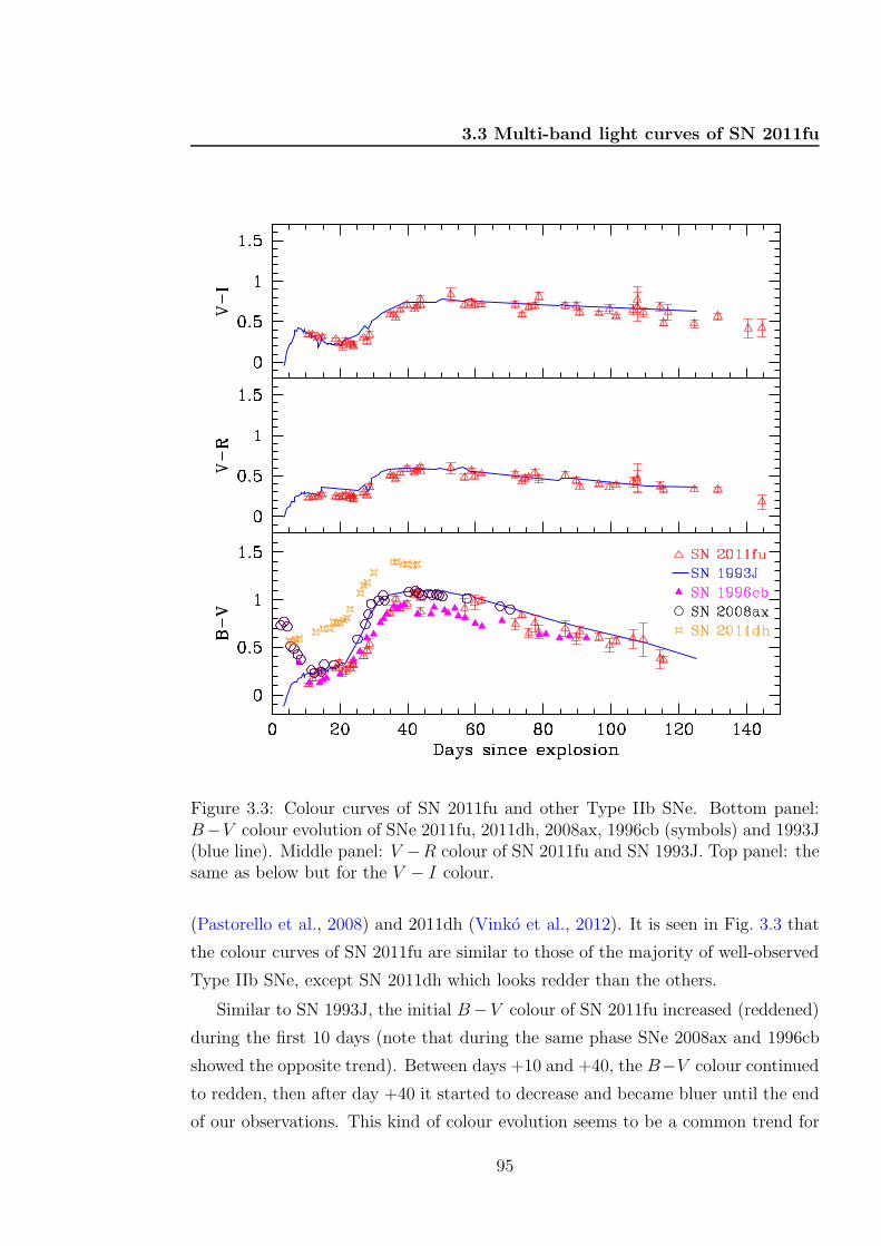
3.3 Multi-band light curves of SN 2011fu
Figure 3.3: Colour curves of SN 2011fu and other Type IIb SNe. Bottom panel:B−V colour evolution of SNe 2011fu, 2011dh, 2008ax, 1996cb (symbols) and 1993J(blue line). Middle panel: V −R colour of SN 2011fu and SN 1993J. Top panel: thesame as below but for the V − I colour.
(Pastorello et al., 2008) and 2011dh (Vinko et al., 2012). It is seen in Fig. 3.3 that
the colour curves of SN 2011fu are similar to those of the majority of well-observed
Type IIb SNe, except SN 2011dh which looks redder than the others.
Similar to SN 1993J, the initial B−V colour of SN 2011fu increased (reddened)
during the first 10 days (note that during the same phase SNe 2008ax and 1996cb
showed the opposite trend). Between days +10 and +40, the B−V colour continued
to redden, then after day +40 it started to decrease and became bluer until the end
of our observations. This kind of colour evolution seems to be a common trend for
95
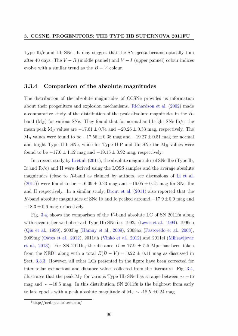
3. CCSNE, PROGENITORS: THE TYPE IIB SUPERNOVA 2011FU
Type Ib/c and IIb SNe. It may suggest that the SN ejecta became optically thin
after 40 days. The V −R (middle pannel) and V − I (upper pannel) colour indices
evolve with a similar trend as the B − V colour.
3.3.4 Comparison of the absolute magnitudes
The distribution of the absolute magnitudes of CCSNe provides us information
about their progenitors and explosion mechanisms. Richardson et al. (2002) made
a comparative study of the distribution of the peak absolute magnitudes in the B-
band (MB) for various SNe. They found that for normal and bright SNe Ib/c, the
mean peak MB values are −17.61± 0.74 and −20.26± 0.33 mag, respectively. The
MB values were found to be −17.56± 0.38 mag and −19.27± 0.51 mag for normal
and bright Type II-L SNe, while for Type II-P and IIn SNe the MB values were
found to be −17.0± 1.12 mag and −19.15± 0.92 mag, respectively.
In a recent study by Li et al. (2011), the absolute magnitudes of SNe Ibc (Type Ib,
Ic and Ib/c) and II were derived using the LOSS samples and the average absolute
magnitudes (close to R-band as claimed by authors, see discussions of Li et al.
(2011)) were found to be −16.09 ± 0.23 mag and −16.05 ± 0.15 mag for SNe Ibc
and II respectively. In a similar study, Drout et al. (2011) also reported that the
R-band absolute magnitudes of SNe Ib and Ic peaked arround −17.9±0.9 mag and
−18.3 ± 0.6 mag respectively.
Fig. 3.4, shows the comparison of the V -band absolute LC of SN 2011fu along
with seven other well-observed Type IIb SNe i.e. 1993J (Lewis et al., 1994), 1996cb
(Qiu et al., 1999), 2003bg (Hamuy et al., 2009), 2008ax (Pastorello et al., 2008),
2009mg (Oates et al., 2012), 2011dh (Vinko et al., 2012) and 2011ei (Milisavljevic
et al., 2013). For SN 2011fu, the distance D = 77.9 ± 5.5 Mpc has been taken
from the NED1 along with a total E(B − V ) = 0.22 ± 0.11 mag as discussed in
Sect. 3.3.3. However, all other LCs presented in the figure have been corrected for
interstellar extinctions and distance values collected from the literature. Fig. 3.4,
illustrates that the peak MV for various Type IIb SNe has a range between ∼ −16
mag and ∼ −18.5 mag. In this distribution, SN 2011fu is the brightest from early
to late epochs with a peak absolute magnitude of MV ∼ -18.5 ±0.24 mag.
1http://ned.ipac.caltech.edu/
96
3.4 Bolometric light curve
Figure 3.4: The MV light curve of SN 2011fu is compared to those of other similarIIb events: SN 2011ei, 2011dh, 2009mg, 2008ax, 2003bg, 1996cb and 1993J.
3.4 Bolometric light curve
3.4.1 Construction of the bolometric light curve
The quasi-bolometric lightcurve (UBVRI ) was computed by integrating the extinction-
corrected flux1 in all 5-bands. The data were interpolated wherever it was necessary
and total UBVRI flux was integrated using a simple trapezoidal rule.
1Fluxes were corrected for interstellar reddening using the idl program ccm unred.pro avail-able at ASTROLIB (http://idlastro.gsfc.nasa.gov/ftp/) by adopting E(B − V ) = 0.22 mag forthe total (Milky Way plus in-host) reddening and by assuming the classical reddening law for thediffused interstellar medium (Rv = 3.1).
97
3. CCSNE, PROGENITORS: THE TYPE IIB SUPERNOVA 2011FU
In Fig. 3.5, we compare the quasi-bolometric LC of SN 2011fu along with other
three Type IIb events i.e. SNe 1993J (Lewis et al., 1994), 2008ax (Pastorello et al.,
2008) and SN 2011dh (Ergon et al., 2014). It is obvious that the shape of the quasi-
bolometric LC of SN 2011fu is similar to that of SN 1993J. However, SN 2011fu is
more luminous in comparison with the other SNe during the observed phases.
The un-observed part of the bolometric LC in the Infra-red was approximated by
assuming blackbody flux distributions fitted to the observed R- and I-band fluxes
for each epoch. At first, we used the Rayleigh-Jeans approximation for the fluxes
redward of the I-band, and integrated the flux distribution between the I-band
central wavelength and infinity. This resulted in an analytic estimate for the IR
(infra-red) contribution as LIR ≈ λI · FI/3, where λI and FI are the I-band central
wavelength and monochromatic flux, respectively. Second, we fitted a blackbody
to the R- and I-band fluxes at each epoch, and numerically integrated the fitted
blackbody flux distributions from the I-band to radio wavelengths (∼ 1 mm). These
two estimates gave consistent results within a few percent, which convinced us that
they are more-or-less realistic estimates of the IR-contribution. Because the R-band
fluxes may also be affected by the presence of Hα, we adopted the result of the first,
analytic estimate as the final result. Comparison of the integrated UBVRI - and
IR-fluxes showed that the IR-contribution was ∼ 20 percent at the earliest observed
phases, but it increased up to ∼ 50 percent by day +40 and stayed roughly constant
after that.
3.4.2 Bolometric light curve modelling
The bolometric light curve (see Sect. 3.4.1) was fitted by the semi-analytic light
curve model of Arnett & Fu (1989) (see also Chatzopoulos et al., 2009). This model
assumes homologously expanding spherical ejecta having a constant opacity, and
solves the photon diffusion equation by taking into account the laws of thermody-
namics. This approach was first introduced by Arnett (1980) and Arnett (1982),
and further extended by Arnett & Fu (1989) by taking into account the rapid change
of the opacity due to recombination. The extended diffusion-recombination model
was succesfully applied to describe the observed light curve of SN 1987A assuming
realistic physical parameters (Arnett & Fu, 1989).
The bolometric LC of SN 2011fu is qualitatively similar to that of SN 1987A,
because of the presence of the rapid initial decline and the secondary bump, after
which the LC settles down onto the radioactive tail due to the 56Co-decay. This
98
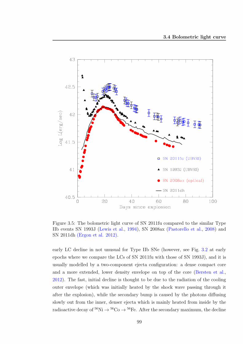
3.4 Bolometric light curve
Figure 3.5: The bolometric light curve of SN 2011fu compared to the similar TypeIIb events SN 1993J (Lewis et al., 1994), SN 2008ax (Pastorello et al., 2008) andSN 2011dh (Ergon et al. 2012).
early LC decline in not unusual for Type IIb SNe (however, see Fig. 3.2 at early
epochs where we compare the LCs of SN 2011fu with those of SN 1993J), and it is
usually modelled by a two-component ejecta configuration: a dense compact core
and a more extended, lower density envelope on top of the core (Bersten et al.,
2012). The fast, initial decline is thought to be due to the radiation of the cooling
outer envelope (which was initially heated by the shock wave passing through it
after the explosion), while the secondary bump is caused by the photons diffusing
slowly out from the inner, denser ejecta which is mainly heated from inside by the
radioactive decay of 56Ni→ 56Co→ 56Fe. After the secondary maximum, the decline
99
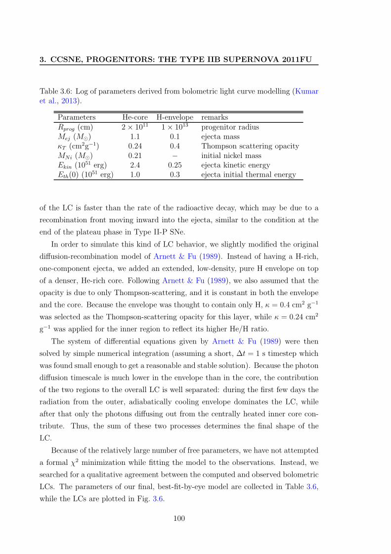
3. CCSNE, PROGENITORS: THE TYPE IIB SUPERNOVA 2011FU
Table 3.6: Log of parameters derived from bolometric light curve modelling (Kumaret al., 2013).
Parameters He-core H-envelope remarksRprog (cm) 2× 10¹¹ 1× 10¹³ progenitor radiusMej (M⊙) 1.1 0.1 ejecta massκT (cm2g−1) 0.24 0.4 Thompson scattering opacityMNi (M⊙) 0.21 − initial nickel massEkin (1051 erg) 2.4 0.25 ejecta kinetic energyEth(0) (10
51 erg) 1.0 0.3 ejecta initial thermal energy
of the LC is faster than the rate of the radioactive decay, which may be due to a
recombination front moving inward into the ejecta, similar to the condition at the
end of the plateau phase in Type II-P SNe.
In order to simulate this kind of LC behavior, we slightly modified the original
diffusion-recombination model of Arnett & Fu (1989). Instead of having a H-rich,
one-component ejecta, we added an extended, low-density, pure H envelope on top
of a denser, He-rich core. Following Arnett & Fu (1989), we also assumed that the
opacity is due to only Thompson-scattering, and it is constant in both the envelope
and the core. Because the envelope was thought to contain only H, κ = 0.4 cm2 g−1
was selected as the Thompson-scattering opacity for this layer, while κ = 0.24 cm2
g−1 was applied for the inner region to reflect its higher He/H ratio.
The system of differential equations given by Arnett & Fu (1989) were then
solved by simple numerical integration (assuming a short, ∆t = 1 s timestep which
was found small enough to get a reasonable and stable solution). Because the photon
diffusion timescale is much lower in the envelope than in the core, the contribution
of the two regions to the overall LC is well separated: during the first few days the
radiation from the outer, adiabatically cooling envelope dominates the LC, while
after that only the photons diffusing out from the centrally heated inner core con-
tribute. Thus, the sum of these two processes determines the final shape of the
LC.
Because of the relatively large number of free parameters, we have not attempted
a formal χ2 minimization while fitting the model to the observations. Instead, we
searched for a qualitative agreement between the computed and observed bolometric
LCs. The parameters of our final, best-fit-by-eye model are collected in Table 3.6,
while the LCs are plotted in Fig. 3.6.
100
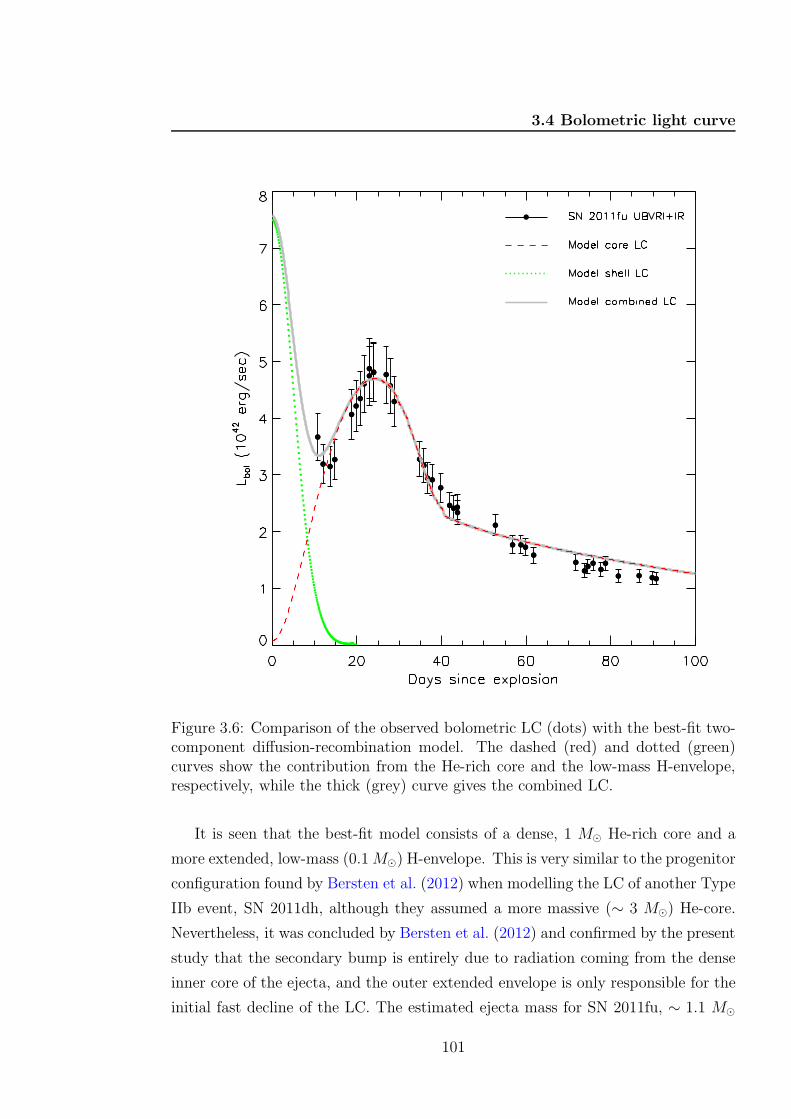
3.4 Bolometric light curve
Figure 3.6: Comparison of the observed bolometric LC (dots) with the best-fit two-component diffusion-recombination model. The dashed (red) and dotted (green)curves show the contribution from the He-rich core and the low-mass H-envelope,respectively, while the thick (grey) curve gives the combined LC.
It is seen that the best-fit model consists of a dense, 1 M⊙ He-rich core and a
more extended, low-mass (0.1M⊙) H-envelope. This is very similar to the progenitor
configuration found by Bersten et al. (2012) when modelling the LC of another Type
IIb event, SN 2011dh, although they assumed a more massive (∼ 3 M⊙) He-core.
Nevertheless, it was concluded by Bersten et al. (2012) and confirmed by the present
study that the secondary bump is entirely due to radiation coming from the dense
inner core of the ejecta, and the outer extended envelope is only responsible for the
initial fast decline of the LC. The estimated ejecta mass for SN 2011fu, ∼ 1.1 M⊙
101
3. CCSNE, PROGENITORS: THE TYPE IIB SUPERNOVA 2011FU
is consistent with the observed rise time (∼ 24 days) to the secondary maximum of
the LC (see Eq.10 of Chatzopoulos et al., 2012). The parameters in Table 3.6 are
also qualitatively similar to the ones derived by Young et al. (1995) for modelling
the LC of SN 1993J.
There are a number of caveats in the simple diffusion-recombination model used
above, which naturally limit the accuracy of the derived physical parameters. The
most obvious limitation is the assumption of constant opacity in the ejecta. The
pre-selected density and temperature profiles in the ejecta (assumed as exponential
functions) are also strong simplifications, but they enable the approximate, semi-
analytic treatment of the complex problem of radiative diffusion, as shown by Arnett
& Fu (1989). Thus, the parameters in Table 3.6 can be considered only as order-of-
magnitude estimates, which could be significantly improved by more sophisticated
modelling codes (e.g. Bersten et al., 2012).
3.5 Spectral analysis
Properties of the SN 2011fu ejecta were investigated with the multi-parametric reso-
nance scattering code SYNOW (Fisher et al., 1997) (see also Baron et al., 2005; Branch
et al., 2002; Elmhamdi et al., 2006). The evolution of temperature and velocities
of layers were traced through several months of spectral observations. The SYNOW
code is based on several assumptions: spherical symmetry; homologous expansion of
layers (v ∼ r); sharp photosphere producing a blackbody spectrum and associated
with a shock wave at early stages.
3.5.1 Comparison between observed and synthetic spectra
In the photospheric phase the spectral lines with P Cygni profiles are formed by
resonance scattering in a shell above the optically thick photosphere which produces
the continuum (see Branch et al., 2001). On the other hand, during the nebular
phase the ejecta is transparent (optically thin) in the optical wavelength range. In
this case the spectrum is dominated by strong emission features including forbidden
lines. Each of these two phases of SN evolution can be explained with individual
approximations and the modelling of the observed spectra should be generated with
different synthetic codes. There is no sharp boundary between these two phases.
No strong transition to the nebular phase with conspicuous emission features can be
seen in the observed spectra of SN 2011fu (Fig. 3.7). The shape of the lines remains
102
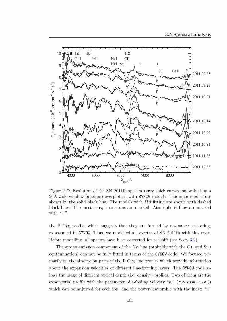
3.5 Spectral analysis
4000 5000 6000 7000 8000λ
rest, A
0
1
2
3
4
5
6
7
8
9
10F
λ + c
onst
. [ 1
0-16 , e
rg c
m-2
A-1
s-1
]
2011.12.22
2011.11.23
2011.10.31
2011.10.29
2011.10.14
2011.10.01
2011.09.29
2011.09.28CaIIOI
HαCII
SiIINaIHeI
HβFeII
TiIIFeII
CaII
++
Figure 3.7: Evolution of the SN 2011fu spectra (grey thick curves, smoothed by a20A-wide window function) overplotted with SYNOW models. The main models areshown by the solid black line. The models with Hβ fitting are shown with dashedblack lines. The most conspicuous ions are marked. Atmospheric lines are markedwith “+”.
the P Cyg profile, which suggests that they are formed by resonance scattering,
as assumed in SYNOW. Thus, we modelled all spectra of SN 2011fu with this code.
Before modelling, all spectra have been corrected for redshift (see Sect. 3.2).
The strong emission component of the Hα line (probably with the C ii and Si ii
contamination) can not be fully fitted in terms of the SYNOW code. We focused pri-
marily on the absorption parts of the P Cyg line profiles which provide information
about the expansion velocities of different line-forming layers. The SYNOW code al-
lows the usage of different optical depth (i.e. density) profiles. Two of them are the
exponential profile with the parameter of e-folding velocity “ve” (τ ∝ exp(−v/ve))
which can be adjusted for each ion, and the power-law profile with the index “n”
103
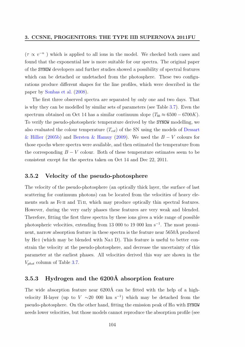
3. CCSNE, PROGENITORS: THE TYPE IIB SUPERNOVA 2011FU
(τ ∝ v−n ) which is applied to all ions in the model. We checked both cases and
found that the exponential law is more suitable for our spectra. The original paper
of the SYNOW developers and further studies showed a possibility of spectral features
which can be detached or undetached from the photosphere. These two configu-
rations produce different shapes for the line profiles, which were described in the
paper by Sonbas et al. (2008).
The first three observed spectra are separated by only one and two days. That
is why they can be modelled by similar sets of parameters (see Table 3.7). Even the
spectrum obtained on Oct 14 has a similar continuum slope (Tbb ≈ 6500− 6700K).
To verify the pseudo-photospheric temperature derived by the SYNOW modelling, we
also evaluated the colour temperature (Tcol) of the SN using the models of Dessart
& Hillier (2005b) and Bersten & Hamuy (2009). We used the B − V colours for
those epochs where spectra were available, and then estimated the temperature from
the corresponding B − V colour. Both of these temperature estimates seem to be
consistent except for the spectra taken on Oct 14 and Dec 22, 2011.
3.5.2 Velocity of the pseudo-photosphere
The velocity of the pseudo-photosphere (an optically thick layer, the surface of last
scattering for continuum photons) can be located from the velocities of heavy ele-
ments such as Fe ii and Ti ii, which may produce optically thin spectral features.
However, during the very early phases these features are very weak and blended.
Therefore, fitting the first three spectra by these ions gives a wide range of possible
photospheric velocities, extending from 13 000 to 19 000 km s−1. The most promi-
nent, narrow absorption feature in these spectra is the feature near 5650A produced
by He i (which may be blended with Na i D). This feature is useful to better con-
strain the velocity at the pseudo-photosphere, and decrease the uncertainty of this
parameter at the earliest phases. All velocities derived this way are shown in the
Vphot column of Table 3.7.
3.5.3 Hydrogen and the 6200A absorption feature
The wide absorption feature near 6200A can be fitted with the help of a high-
velocity H-layer (up to V ∼20 000 km s−1) which may be detached from the
pseudo-photosphere. On the other hand, fitting the emission peak of Hα with SYNOW
needs lower velocities, but those models cannot reproduce the absorption profile (see
104
3.5 Spectral analysis
Table 3.7: Velocities of the pseudo-photosphere, Hα and Hβ at different epochsfor SN 2011fu, derived with SYNOW. We assumed that the photospheric velocity(Vphot) is equal to the velocity of Fe ii. All velocities are given in km s−1. Tbb is theblackbody temperature of the pseudo-photosphere in Kelvin degrees. The colourtemperature (Tcol) derived from the effective temperature − colour relations (seeBersten & Hamuy, 2009; Dessart & Hillier, 2005b) is given in the last column.
UT Date Vphot V (Hα) V (Hβ) Tbb Tcol
(yyyy/mm/dd) (Fe II)2011/09/28 14000 16000 16000 6700 69522011/09/29 14000 16000 14000 6500 64762011/10/01 11000 15000 11000 6500 60522011/10/14 8000 11000 8500 6700 57912011/10/29 6200 9500 9500 5000 46982011/10/31 6000 9000 9000 5000 47952011/11/23 6000 9000 9000 5000 50942011/12/22 5000 9000 9000 5000 5718
Fig. 3.7). In the V (Hα) column of Table 3.7 we list the results from the latter, more
conservative solution.
The broad absorption at 6200A can be also explained with the presence of the
C ii ion having a high-velocity almost identical to that of Hα. Moreover, C ii also
produces a small feature near 4400A. This feature can constrain the reference optical
depth (τ) for ionized carbon. But the contamination from heavy elements in the
blue region makes the fitting of the C ii 4400A feature uncertain. Thus, the presence
of carbon cannot be confirmed from these spectra.
It is also possible to explain the 6200A feature by singly ionized silicon. In this
case the velocity of Si ii must be very low. On the other hand, it is expected that
the velocity of Si ii should be equal or only slightly higher than the photospheric
velocity. It turned out that only the blue wing of this wide feature can be fitted by
Si ii. Although the small absorption near 5880 A might be explained by the presence
of Si ii, the observed shape of the 6200A feature does not confirm this hypothesis.
In order to look for other possibilities, we also checked different blends of H,
Si ii, C ii and some other ions with different velocities (assuming undetached as
well as detached line formation) in our models. At the early phases the range
of derived velocities turned out to be wide due to the lack of observable spectral
features formed close to the photosphere, as discussed above. At the late phases, the
wide absorption near 6200A splitted into at least three separate features (6100A,
6200A, 6350A). These features might be explained as a line formation effect for
Hα in layers with different velocities or the appearance of blending due to the ions
105
3. CCSNE, PROGENITORS: THE TYPE IIB SUPERNOVA 2011FU
Figure 3.8: Evolution of Hα, Hβ and Fe ii line velocities by fitting the SYNOW model(see Table 3.7). The photospheric velocities for SN 2011fu, 2003bg (Hamuy et al.,2009), 1993J (Barbon et al., 1995; Lewis et al., 1994) and 2008ax (Pastorello et al.,2008) are shown. The symbols of SN 2011fu are connected with lines, those of otherSNe with dotted lines.
mentioned above. Unfortunately, no firm conclusion can be drawn based on the
simple parametric models that SYNOW can produce.
The deep absorption near 4700A can be naturally explained identifying it as the
Hβ line. We fitted this line and the Hα line independently because they cannot
be modeled by the same set of parameters: τ , vphot and ve (see also Quimby et al.,
2007). From Table 3.7 it is visible that for the spectra obtained before Oct 29 the
fitting of Hα needs higher velocities than the fitting of Hβ. Although both the Hα
and Hβ velocities declined in time, the formation of the absorption component of
Hα stayed at higher velocities than for Hβ. This may suggest that Hα remained
optically thick for a longer time than Hβ in the expanding, diluting H-rich envelope.
106
3.5 Spectral analysis
3.5.4 Other ions
To fit the main features in the spectra, we included the following elements and ions
in SYNOW: H, Fe ii, Ti ii, Na i, Si ii, O i and Ca ii. Some models were also computed
containing the following elements and ions as alternatives: C ii, He i, Fe i, Ti i, Sc ii,
Mg i and the consistency of these ions were cross-examined with Hatano et al. (1999).
The heavier atoms/ions should have velocities close to vphot but the lighter ones may
be detached due to e.g. stratification of elements in the ejecta.
In the following, we show some possibilities to explain these features in the
observed spectra. Weak features near 4810A and 6370A can be explained by the
presence of low-velocity He i. He can also be found as a blend with Na i in the deep
absorption near 5650A mentioned above, and as a blend with Ti ii and Fe ii near
4300A. However, the velocity of He i may be higher than the photospheric velocity.
Even in this case, the presence of He can explain all these features.
A small absorption in the blue wing of Hα at 6630A could be modeled by He i
or low-velocity C ii. The feature near 5050A could be fitted with Mg i as well. The
Ca ii H+K feature cannot be fitted well around 3730A, because this regime is at the
blue end of our observed spectra and all of them are very noisy at these wavelengths.
But the absorption feature near 8400A is compatible with the Ca ii IR-triplet.
3.5.5 Results of spectral modelling
Almost all spectral features are well described with elements and ions which are
usually applied to the case of Type IIb SNe. However, the strong emission of Hα
dominating during some intermediate epochs cannot be fully fitted with the models
applied.
The fitting of redder and especially bluer parts has some uncertainties due to
strong blending of metal lines such as Ca ii, Ti ii, Fe ii and others. Even without
a precise modelling, all spectral sequences can be divided into two groups: the
first four spectra (up to Oct 14) which are fitted with models with the blackbody
temperature Tbb ≈ 6500 - 6700 K and the following four spectra with Tbb ≈ 5000 K.
Generally, the modelling of the SN 2011fu spectra shows a decline of the pho-
tospheric velocities up to ∼ 40 days after the explosion (see Fig. 3.8). Then, all
velocities remain approximately at the same, stable level. This behaviour was also
described in previous works on CCSNe (Branch et al., 2002; Moskvitin et al., 2010;
107
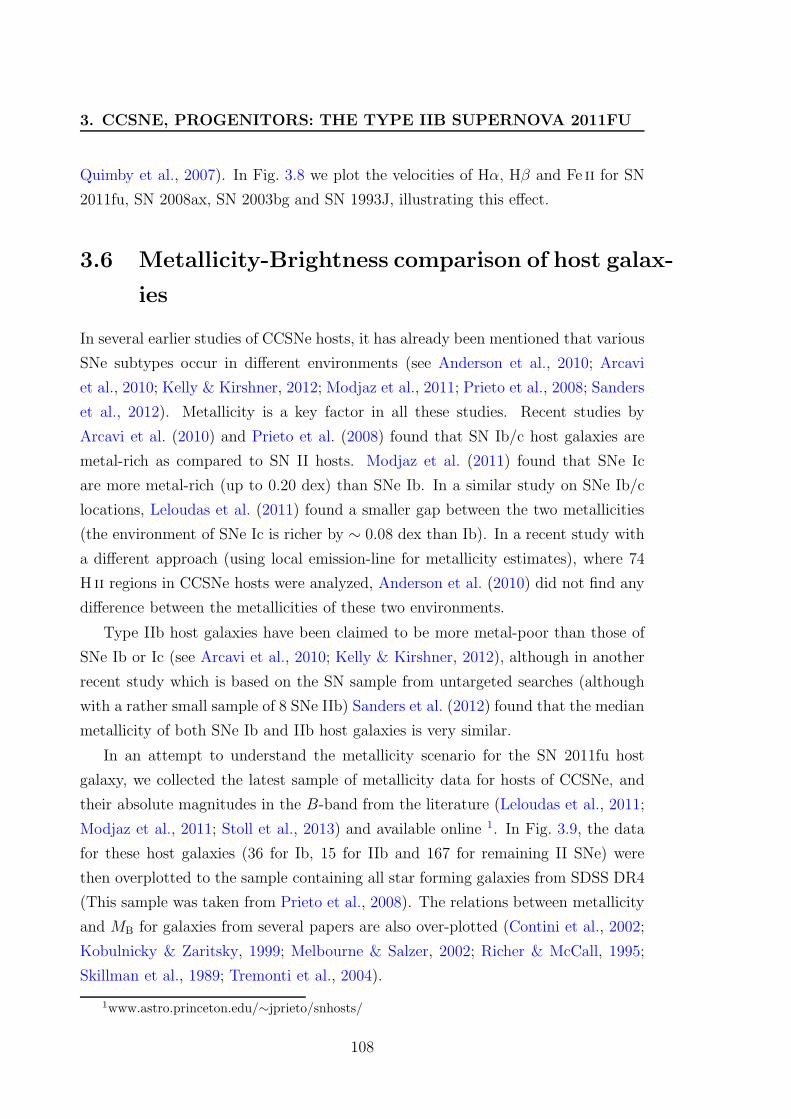
3. CCSNE, PROGENITORS: THE TYPE IIB SUPERNOVA 2011FU
Quimby et al., 2007). In Fig. 3.8 we plot the velocities of Hα, Hβ and Fe ii for SN
2011fu, SN 2008ax, SN 2003bg and SN 1993J, illustrating this effect.
3.6 Metallicity-Brightness comparison of host galax-
ies
In several earlier studies of CCSNe hosts, it has already been mentioned that various
SNe subtypes occur in different environments (see Anderson et al., 2010; Arcavi
et al., 2010; Kelly & Kirshner, 2012; Modjaz et al., 2011; Prieto et al., 2008; Sanders
et al., 2012). Metallicity is a key factor in all these studies. Recent studies by
Arcavi et al. (2010) and Prieto et al. (2008) found that SN Ib/c host galaxies are
metal-rich as compared to SN II hosts. Modjaz et al. (2011) found that SNe Ic
are more metal-rich (up to 0.20 dex) than SNe Ib. In a similar study on SNe Ib/c
locations, Leloudas et al. (2011) found a smaller gap between the two metallicities
(the environment of SNe Ic is richer by ∼ 0.08 dex than Ib). In a recent study with
a different approach (using local emission-line for metallicity estimates), where 74
H ii regions in CCSNe hosts were analyzed, Anderson et al. (2010) did not find any
difference between the metallicities of these two environments.
Type IIb host galaxies have been claimed to be more metal-poor than those of
SNe Ib or Ic (see Arcavi et al., 2010; Kelly & Kirshner, 2012), although in another
recent study which is based on the SN sample from untargeted searches (although
with a rather small sample of 8 SNe IIb) Sanders et al. (2012) found that the median
metallicity of both SNe Ib and IIb host galaxies is very similar.
In an attempt to understand the metallicity scenario for the SN 2011fu host
galaxy, we collected the latest sample of metallicity data for hosts of CCSNe, and
their absolute magnitudes in the B-band from the literature (Leloudas et al., 2011;
Modjaz et al., 2011; Stoll et al., 2013) and available online 1. In Fig. 3.9, the data
for these host galaxies (36 for Ib, 15 for IIb and 167 for remaining II SNe) were
then overplotted to the sample containing all star forming galaxies from SDSS DR4
(This sample was taken from Prieto et al., 2008). The relations between metallicity
and MB for galaxies from several papers are also over-plotted (Contini et al., 2002;
Kobulnicky & Zaritsky, 1999; Melbourne & Salzer, 2002; Richer & McCall, 1995;
Skillman et al., 1989; Tremonti et al., 2004).
1www.astro.princeton.edu/∼jprieto/snhosts/
108
3.6 Metallicity-Brightness comparison of host galaxies
Figure 3.9: Metallicity-luminosity relation for various types of SNe host galaxies.The tiny dots belong to all galaxies used by Prieto et al. (2008) (This catalog isbased on SDSS DR4 Adelman-McCarthy et al., 2006, database). Red squares refereto Type II, stars to Type Ib/c and black dots to Type IIb SNe, respectively. Theanalytic relations collected from several papers (see text) are also over-plotted. TheSN 2011fu host metallicity is denoted by a black triangle.
We estimated the metallicity of the host of SN 2011fu using the relation given by
Garnett (2002) (see their equation 6). We considered MB = −20.62 mag for UGC
01626 from HyperLeda. The calculated log(O/H) + 12 for UGC 01626 is 8.90+0.10−0.06.
This value is slightly higher than log(O/H) + 12 = 8.55 (Arcavi et al., 2010) and
log(O/H)+12 = 8.44 (Sanders et al., 2012) for the SN type II sample. Our analysis
using the most updated sample of absolute magnitudes and metallicities of CCSNe
host galaxies also supports the results described in Sanders et al. (2012). However,
it is noticeable that methods used to determine metallicities are based on statistical
samples, affected by incompleteness of the sample and should be used with caution.
109
3. CCSNE, PROGENITORS: THE TYPE IIB SUPERNOVA 2011FU
3.7 Conclusions
We present a comprehensive UBVRI photometric and low-resolution spectroscopic
monitoring of the Type IIb SN 2011fu. To date, only a handful of SNe belonging to
this class have been observed and studied in detail.
To the best of our knowledge, our photometric and spectroscopic observations
described here are the earliest ones reported for this event. The early photometric
observations strongly suggest the presence of the early-time decline of the light
curve (which is thought to be related to the shock break-out phase) as seen in case
of SN 1993J. The early-time LC decay rate (α1) of this SN is slower than that derived
for SN 1993J in all the bands. The rising rates between the LC valley to peak (α2)
observed in SN 2011fu is also somewhat slower than in SN 1993J. However, the post
peak LC decay rate (α3) are similar in the two events.
The colour evolution of SN 2011fu was studied using our UBVRI band obser-
vations. Our data showed that during the very early phases the B − V colour was
very similar to that of SN 1993J. A similar trend has been found in the V −R and
V − I colours as well. The evolution of these three colours after +40 days were also
similar to those seen in other CCSNe. The V -band absolute magnitudes of a sam-
ple of 8 Type IIb SNe were compared after applying proper extinction corrections
and taking into account distances collected from the literature. In this sample, SN
2011fu seems to be the most luminous event. However, the peak V -band absolute
magnitude of SN 2011fu is not an outlier when it is compared to the peak brightness
of CCSNe of other types.
The quasi-bolometric LC of SN 2011fu was assembled using our UBVRI data
and accounting for the IR contribution as specified in Section 3.4. Comparison
of these data with other known Type IIb SNe also shows that SN 2011fu is the
brightest Type IIb SN in the sample. The bolometric LC was modeled by applying
a semi-analytical model of Arnett & Fu (1989). This model suggests a 1.1 M⊙
He-rich core and an extended, low-mass (∼ 0.1 M⊙) H-envelope as the progenitor
of SN 2011fu, similar to that of SN 2011dh. However, the progenitor radius of
SN 2011fu (∼ 1 × 1013 cm) turned out to be smaller than that of SN 1993J (∼4 × 1013 cm) (Woosley et al., 1994). The ejected nickel mass for SN 2011fu was
∼ 0.21 M⊙, higher than that of SN 1993J (0.07 − 0.11 M⊙).
The spectra of SN 2011fu taken at eight epochs were analyzed using the multi-
parameter resonance scattering code SYNOW. The derived parameters describe the
110
3.7 Conclusions
evolution of the velocities related to various atoms/ions and the variation of the
blackbody temperature of the pseudo-photosphere. The photospheric velocities at
the early epochs were higher than those of other Type IIb SNe. The pseudo photo-
spheric temperatures were found to be between 6700 K and 5000 K, decreasing from
initial to later phases. The temperatures from SYNOW were also checked by compar-
ing them with colour temperatures calculated from B−V vs Teff relations (Bersten
& Hamuy, 2009; Dessart & Hillier, 2005b). These different temperature estimates
were found to be consistent. The appearance of the main observed spectral features
was also successfully modeled with SYNOW by assuming H, He i and various metals
(mostly Fe ii, Ti ii and Ca ii), which are typical of CCSNe spectra. The estimated
value of the metallicity of the host galaxy of SN 2011fu is 8.90+0.10−0.06 similar to those
for other Type IIb SNe.
111

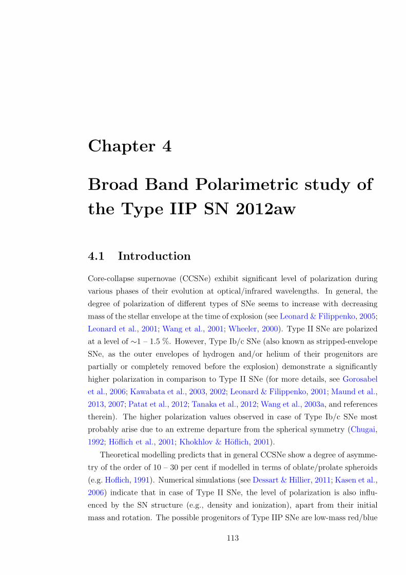
Chapter 4
Broad Band Polarimetric study of
the Type IIP SN 2012aw
4.1 Introduction
Core-collapse supernovae (CCSNe) exhibit significant level of polarization during
various phases of their evolution at optical/infrared wavelengths. In general, the
degree of polarization of different types of SNe seems to increase with decreasing
mass of the stellar envelope at the time of explosion (see Leonard & Filippenko, 2005;
Leonard et al., 2001; Wang et al., 2001; Wheeler, 2000). Type II SNe are polarized
at a level of ∼1 – 1.5 %. However, Type Ib/c SNe (also known as stripped-envelope
SNe, as the outer envelopes of hydrogen and/or helium of their progenitors are
partially or completely removed before the explosion) demonstrate a significantly
higher polarization in comparison to Type II SNe (for more details, see Gorosabel
et al., 2006; Kawabata et al., 2003, 2002; Leonard & Filippenko, 2001; Maund et al.,
2013, 2007; Patat et al., 2012; Tanaka et al., 2012; Wang et al., 2003a, and references
therein). The higher polarization values observed in case of Type Ib/c SNe most
probably arise due to an extreme departure from the spherical symmetry (Chugai,
1992; Hoflich et al., 2001; Khokhlov & Hoflich, 2001).
Theoretical modelling predicts that in general CCSNe show a degree of asymme-
try of the order of 10 – 30 per cent if modelled in terms of oblate/prolate spheroids
(e.g. Hoflich, 1991). Numerical simulations (see Dessart & Hillier, 2011; Kasen et al.,
2006) indicate that in case of Type II SNe, the level of polarization is also influ-
enced by the SN structure (e.g., density and ionization), apart from their initial
mass and rotation. The possible progenitors of Type IIP SNe are low-mass red/blue
113
4. BROAD BAND POLARIMETRIC STUDY OF THE TYPE IIPSN 2012AW
supergiants and their polarization studies are extremely useful to understand the SN
structure in detail. In spite of being the most common subtypes among the known
CCSNe, polarization studies of Type IIP SNe have only been done for a handful of
cases (e.g. Barrett, 1988; Chornock et al., 2010; Chugai, 2006; Leonard et al., 2012a;
Leonard & Filippenko, 2001; Leonard et al., 2001, 2006). In general, intrinsic po-
larization in these SNe is observed below 1 per cent but a few exceptions exist in
the literature (for example Chornock et al. (2010) reported ∼1.5% for SN 2006ov).
Systematic polarimetric studies have been started, only after the observations of
Type IIP SN 1987A (see Cropper et al., 1988; Jeffery, 1991; Mendez et al., 1988).
Shapiro & Sutherland (1982) first pointed out that polarimetry provides direct pow-
erful probe to understand the SN geometry (see also Hoflich, 1991; McCall, 1984).
Polarization is believed to be produced due to electron scattering within the SN
ejecta. When light passes through the expanding ejecta of CCSNe, it retains infor-
mation about the orientation of the layers. In the spherically symmetric scenario,
the equally present directional components of the electric vectors will be canceled
out to produce a zero net polarization. If the source is aspherical, incomplete can-
cellation occurs which finally imprints a net polarization (see Fig. 1 of Filippenko
& Leonard 2004 and Leonard & Filippenko 2005). In addition to asphericity of the
electron scattering atmosphere, there are several other processes which can produce
polarization in CCSNe such as scattering by dust (e.g. Wang & Wheeler, 1996),
clumpy ejecta or asymmetrically distributed radioactive material within the SN en-
velope (e.g. Chugai, 2006; Hoeflich, 1995), and aspherical ionization produced by
hard X−rays from the interaction between the SN shock front and a non-spherical
progenitor wind (Wheeler & Filippenko, 1996).
To diagnose the underlying polarization in SNe explosions, two basic techniques
i.e. broad-band polarimetry and spectropolarimetry have been used. Both of these
techniques have advantages and disadvantages relative to each other. One of the
main advantages of spectropolarimetry of SNe with respect to broad-band polarime-
try is its ability to infer geometric and dynamical information for the different chem-
ical constituents of the explosion. Broad-band polarimetric observations construct
a rather rough picture of the stellar death but require a lesser number of total pho-
tons than spectropolarimetry. Hence broad-band polarimetric observations can be
extended to objects at higher red-shifts or/and allow to enhance the polarimetric
coverage and sampling of the light curve (LC), especially at epochs far from the
maximum when the SN is dimmer.
114
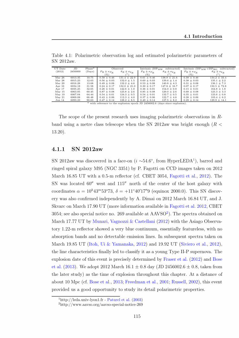
4.1 Introduction
Table 4.1: Polarimetric observation log and estimated polarimetric parameters ofSN 2012aw.
UT Date JD Phasea Observed Intrinsic (ISPMW subtracted) Intrinsic (ISPMW+ISPHG subtracted)(2012) 2450000 (Days) PR ± σPR
θR ± σθRPR ± σPR
θR ± σθRPR ± σPR
θR ± σθR
(%) () (%) () (%) ()Mar 26 6013.35 10.75 0.58 ± 0.46 131.4 ± 22.9 0.61 ± 0.46 138.9 ± 21.6 0.39 ± 0.46 134.2 ± 33.4Mar 28 6015.23 12.63 0.56 ± 0.03 132.0 ± 1.5 0.60 ± 0.03 139.6 ± 1.4 0.38 ± 0.03 135.1 ± 2.2Mar 29 6016.28 13.68 0.49 ± 0.08 132.2 ± 4.6 0.53 ± 0.08 140.8 ± 4.3 0.31 ± 0.08 136.1 ± 7.3Apr 16 6034.18 31.58 0.24 ± 0.17 132.0 ± 21.0 0.30 ± 0.17 147.8 ± 16.7 0.07 ± 0.17 150.5 ± 72.8Apr 17 6035.25 32.65 0.26 ± 0.01 142.6 ± 1.0 0.36 ± 0.01 154.0 ± 0.8 0.15 ± 0.01 164.8 ± 1.8May 15 6063.05 60.45 0.87 ± 0.08 123.8 ± 2.6 0.85 ± 0.08 129.0 ± 2.6 0.68 ± 0.08 123.3 ± 3.3May 19 6067.04 64.44 0.54 ± 0.01 124.3 ± 0.5 0.54 ± 0.01 132.7 ± 0.5 0.35 ± 0.01 123.6 ± 0.8May 21 6069.08 66.48 0.43 ± 0.06 112.3 ± 4.0 0.37 ± 0.06 122.7 ± 4.6 0.28 ± 0.06 103.4 ± 6.2Jun 14 6093.23 90.63 0.47 ± 0.14 128.2 ± 8.5 0.49 ± 0.14 137.5 ± 8.2 0.29 ± 0.14 129.9 ± 14.1
a with reference to the explosion epoch JD 2456002.6 (days since explosion).
The scope of the present research uses imaging polarimetric observations in R-
band using a metre class telescope when the SN 2012aw was bright enough (R <
13.20).
4.1.1 SN 2012aw
SN 2012aw was discovered in a face-on (i ∼54.6, from HyperLEDA1), barred and
ringed spiral galaxy M95 (NGC 3351) by P. Fagotti on CCD images taken on 2012
March 16.85 UT with a 0.5-m reflector (cf. CBET 3054, Fagotti et al., 2012). The
SN was located 60′′ west and 115′′ north of the center of the host galaxy with
coordinates α = 10h43m53s73, δ = +1140′17′′9 (equinox 2000.0). This SN discov-
ery was also confirmed independently by A. Dimai on 2012 March 16.84 UT, and J.
Skvarc on March 17.90 UT (more information available in Fagotti et al. 2012, CBET
3054; see also special notice no. 269 available at AAVSO2). The spectra obtained on
March 17.77 UT by Munari, Vagnozzi & Castellani (2012) with the Asiago Observa-
tory 1.22-m reflector showed a very blue continuum, essentially featureless, with no
absorption bands and no detectable emission lines. In subsequent spectra taken on
March 19.85 UT (Itoh, Ui & Yamanaka, 2012) and 19.92 UT (Siviero et al., 2012),
the line characteristics finally led to classify it as a young Type II-P supernova. The
explosion date of this event is precisely determined by Fraser et al. (2012) and Bose
et al. (2013). We adopt 2012 March 16.1 ± 0.8 day (JD 2456002.6 ± 0.8, taken from
the later study) as the time of explosion throughout this chapter. At a distance of
about 10 Mpc (cf. Bose et al., 2013; Freedman et al., 2001; Russell, 2002), this event
provided us a good opportunity to study its detail polarimetric properties.
1http://leda.univ-lyon1.fr - Paturel et al. (2003)2http://www.aavso.org/aavso-special-notice-269
115
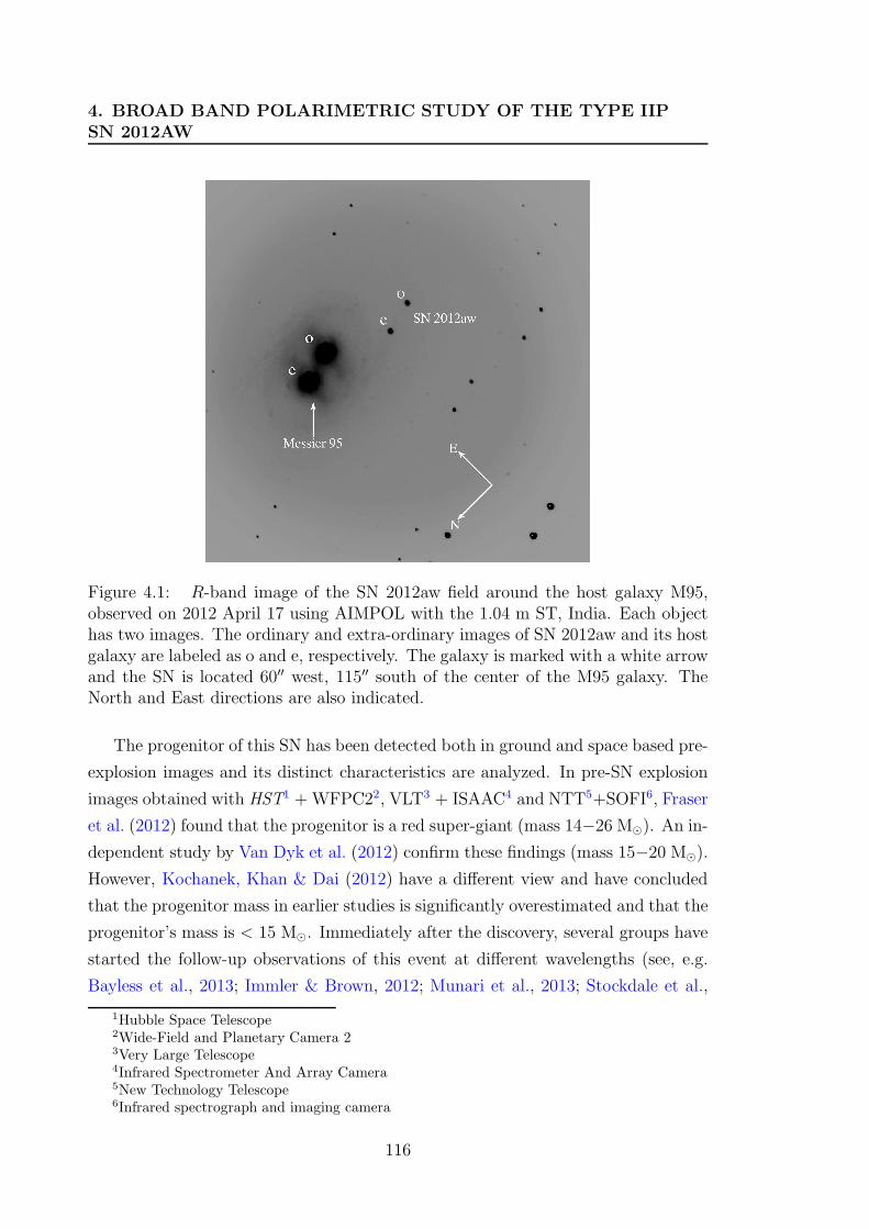
4. BROAD BAND POLARIMETRIC STUDY OF THE TYPE IIPSN 2012AW
Figure 4.1: R-band image of the SN 2012aw field around the host galaxy M95,observed on 2012 April 17 using AIMPOL with the 1.04 m ST, India. Each objecthas two images. The ordinary and extra-ordinary images of SN 2012aw and its hostgalaxy are labeled as o and e, respectively. The galaxy is marked with a white arrowand the SN is located 60′′ west, 115′′ south of the center of the M95 galaxy. TheNorth and East directions are also indicated.
The progenitor of this SN has been detected both in ground and space based pre-
explosion images and its distinct characteristics are analyzed. In pre-SN explosion
images obtained with HST1 +WFPC22, VLT3 + ISAAC4 and NTT5+SOFI6, Fraser
et al. (2012) found that the progenitor is a red super-giant (mass 14−26 M⊙). An in-
dependent study by Van Dyk et al. (2012) confirm these findings (mass 15−20 M⊙).
However, Kochanek, Khan & Dai (2012) have a different view and have concluded
that the progenitor mass in earlier studies is significantly overestimated and that the
progenitor’s mass is < 15 M⊙. Immediately after the discovery, several groups have
started the follow-up observations of this event at different wavelengths (see, e.g.
Bayless et al., 2013; Immler & Brown, 2012; Munari et al., 2013; Stockdale et al.,
1Hubble Space Telescope2Wide-Field and Planetary Camera 23Very Large Telescope4Infrared Spectrometer And Array Camera5New Technology Telescope6Infrared spectrograph and imaging camera
116
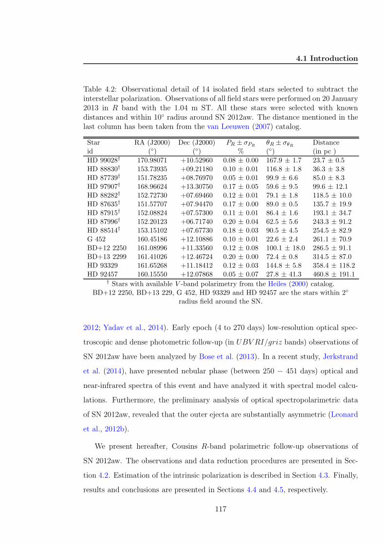
4.1 Introduction
Table 4.2: Observational detail of 14 isolated field stars selected to subtract theinterstellar polarization. Observations of all field stars were performed on 20 January2013 in R band with the 1.04 m ST. All these stars were selected with knowndistances and within 10 radius around SN 2012aw. The distance mentioned in thelast column has been taken from the van Leeuwen (2007) catalog.
Star RA (J2000) Dec (J2000) PR ± σPRθR ± σθR Distance
id () () % () (in pc )
HD 99028† 170.98071 +10.52960 0.08 ± 0.00 167.9 ± 1.7 23.7 ± 0.5HD 88830† 153.73935 +09.21180 0.10 ± 0.01 116.8 ± 1.8 36.3 ± 3.8HD 87739† 151.78235 +08.76970 0.05 ± 0.01 99.9 ± 6.6 85.0 ± 8.3HD 97907† 168.96624 +13.30750 0.17 ± 0.05 59.6 ± 9.5 99.6 ± 12.1HD 88282† 152.72730 +07.69460 0.12 ± 0.01 79.1 ± 1.8 118.5 ± 10.0HD 87635† 151.57707 +07.94470 0.17 ± 0.00 89.0 ± 0.5 135.7 ± 19.9HD 87915† 152.08824 +07.57300 0.11 ± 0.01 86.4 ± 1.6 193.1 ± 34.7HD 87996† 152.20123 +06.71740 0.20 ± 0.04 62.5 ± 5.6 243.3 ± 91.2HD 88514† 153.15102 +07.67730 0.18 ± 0.03 90.5 ± 4.5 254.5 ± 82.9G 452 160.45186 +12.10886 0.10 ± 0.01 22.6 ± 2.4 261.1 ± 70.9BD+12 2250 161.08996 +11.33560 0.12 ± 0.08 100.1 ± 18.0 286.5 ± 91.1BD+13 2299 161.41026 +12.46724 0.20 ± 0.00 72.4 ± 0.8 314.5 ± 87.0HD 93329 161.65268 +11.18412 0.12 ± 0.03 144.8 ± 5.8 358.4 ± 118.2HD 92457 160.15550 +12.07868 0.05 ± 0.07 27.8 ± 41.3 460.8 ± 191.1
† Stars with available V -band polarimetry from the Heiles (2000) catalog.BD+12 2250, BD+13 229, G 452, HD 93329 and HD 92457 are the stars within 2
radius field around the SN.
2012; Yadav et al., 2014). Early epoch (4 to 270 days) low-resolution optical spec-
troscopic and dense photometric follow-up (in UBV RI/griz bands) observations of
SN 2012aw have been analyzed by Bose et al. (2013). In a recent study, Jerkstrand
et al. (2014), have presented nebular phase (between 250 − 451 days) optical and
near-infrared spectra of this event and have analyzed it with spectral model calcu-
lations. Furthermore, the preliminary analysis of optical spectropolarimetric data
of SN 2012aw, revealed that the outer ejecta are substantially asymmetric (Leonard
et al., 2012b).
We present hereafter, Cousins R-band polarimetric follow-up observations of
SN 2012aw. The observations and data reduction procedures are presented in Sec-
tion 4.2. Estimation of the intrinsic polarization is described in Section 4.3. Finally,
results and conclusions are presented in Sections 4.4 and 4.5, respectively.
117
4. BROAD BAND POLARIMETRIC STUDY OF THE TYPE IIPSN 2012AW
4.2 Observations and data reduction
Polarimetric observations of SN 2012aw field were carried out during nine nights,
i.e., 26, 28, 29 March; 16, 17 April; 15, 19, 21 May and 12 June 2012 using the ARIES
Imaging Polarimeter (AIMPOL, Rautela et al., 2004) mounted at the Cassegrain
focus of the 104-cm Sampurnanand telescope (ST) at Manora Peak, Nainital. This
telescope is operated by the Aryabhatta Research Institute of Observational sciences
(ARIES), India. A complete log of these observations is presented in Table 4.1. The
position of the SN, which is fairly isolated from the host galaxy and lies on a smooth
and faint galaxy background is shown in Fig. 4.1. The observations were carried
out in the R (λReff= 0.67µm) photometric band using a liquid nitrogen cooled
Tektronix 1024 × 1024 pixel2 CCD camera. Each pixel of the CCD corresponds
to 1.73 arcsec and the field-of-view (FOV) is ∼8 arcmin in diameter on the sky.
The full width at half-maximum of the stellar images vary from 2 to 3 pixels. The
readout noise and the gain of the CCD are 7.0 e− and 11.98 e−/ADU respectively.
Fig. 4.2 illustrates the optical design of AIMPOL. The f/13 beam from the
telescope falls on the field lens (50mm, f/6 Karl Lambrecht part no. 322305) which
in combination with the camera lens (85mm, f /1.8 ) makes the image of the object
on the CCD chip. A rotatable HWP modulator and a Wollaston beam splitter
prism (analyzer) are mounted in between the camera lens and the field lines. The
Wollaston prism provides ordinary and extra-ordinary beams separated by 28 pixels
along the north-south direction on the sky plane. This set-up gives one of the Stoke’s
parameter Q or U . The other Stoke’s parameters can be obtained by rotating the
plane of polarization of the incoming light. This is accomplished by introducing
a HWP. When the half-wave plate is rotated through an angle α, the plane of
polarization rotates through an angle 2α. At this new position of the HWP another
measurement of the orthogonally polarized beams can be made to determine the
second Stoke parameter.
In order to get measurements with a good signal-to-noise ratio for the present
set of observations ratio, the images that were acquired at each position of the half-
wave plate were combined. Since AIMPOL is not equipped with a narrow-window
mask, care was taken to exclude the stars that were contaminated because of the
overlap of their ordinary and extraordinary images with those of another star in the
FOV.
118
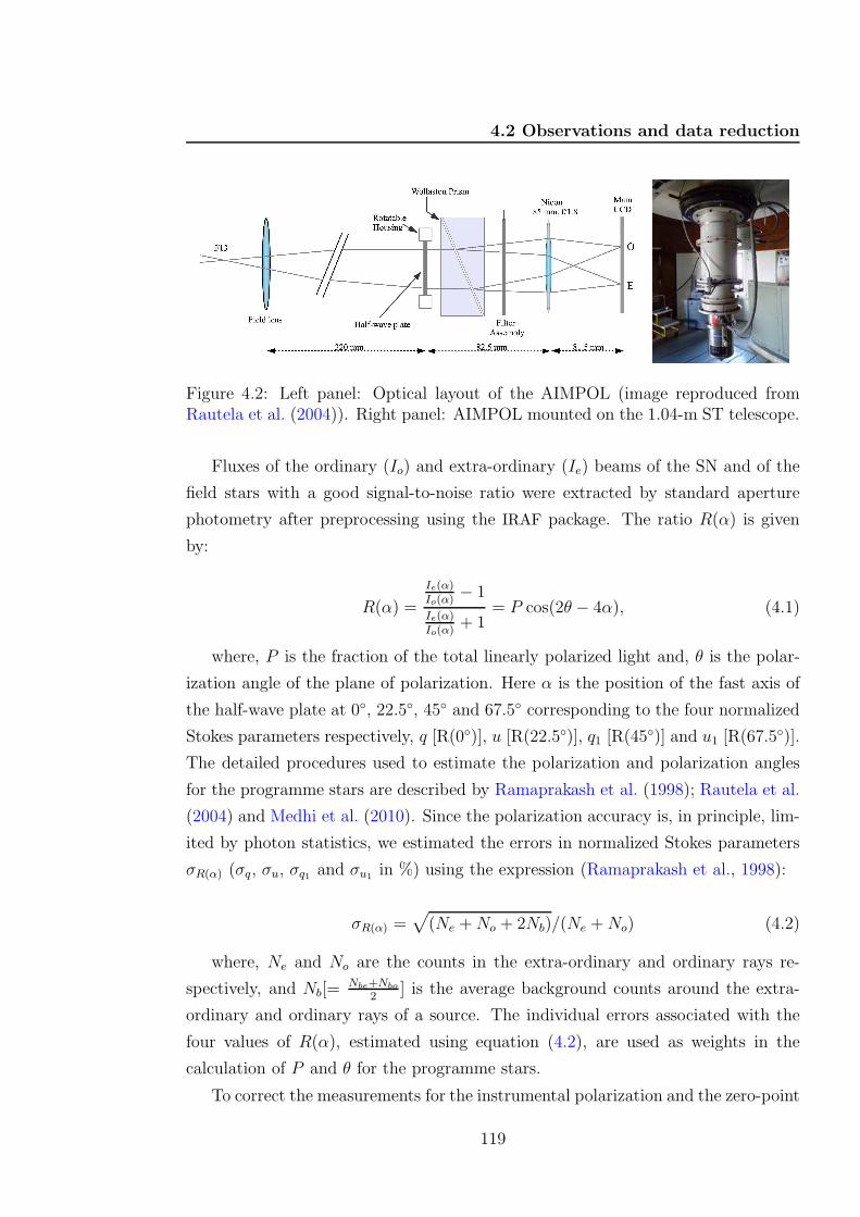
4.2 Observations and data reduction
Figure 4.2: Left panel: Optical layout of the AIMPOL (image reproduced fromRautela et al. (2004)). Right panel: AIMPOL mounted on the 1.04-m ST telescope.
Fluxes of the ordinary (Io) and extra-ordinary (Ie) beams of the SN and of the
field stars with a good signal-to-noise ratio were extracted by standard aperture
photometry after preprocessing using the IRAF package. The ratio R(α) is given
by:
R(α) =
Ie(α)Io(α)
− 1
Ie(α)Io(α)
+ 1= P cos(2θ − 4α), (4.1)
where, P is the fraction of the total linearly polarized light and, θ is the polar-
ization angle of the plane of polarization. Here α is the position of the fast axis of
the half-wave plate at 0, 22.5, 45 and 67.5 corresponding to the four normalized
Stokes parameters respectively, q [R(0)], u [R(22.5)], q1 [R(45)] and u1 [R(67.5
)].
The detailed procedures used to estimate the polarization and polarization angles
for the programme stars are described by Ramaprakash et al. (1998); Rautela et al.
(2004) and Medhi et al. (2010). Since the polarization accuracy is, in principle, lim-
ited by photon statistics, we estimated the errors in normalized Stokes parameters
σR(α) (σq, σu, σq1 and σu1 in %) using the expression (Ramaprakash et al., 1998):
σR(α) =√
(Ne +No + 2Nb)/(Ne +No) (4.2)
where, Ne and No are the counts in the extra-ordinary and ordinary rays re-
spectively, and Nb[=Nbe+Nbo
2] is the average background counts around the extra-
ordinary and ordinary rays of a source. The individual errors associated with the
four values of R(α), estimated using equation (4.2), are used as weights in the
calculation of P and θ for the programme stars.
To correct the measurements for the instrumental polarization and the zero-point
119
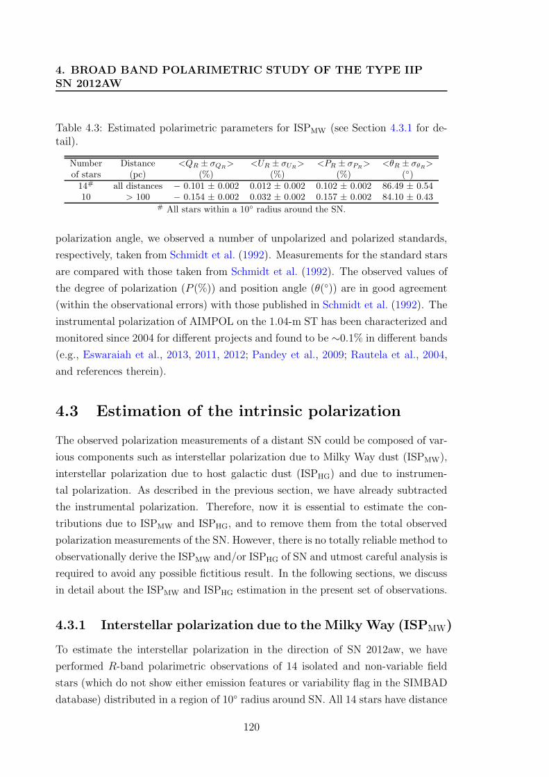
4. BROAD BAND POLARIMETRIC STUDY OF THE TYPE IIPSN 2012AW
Table 4.3: Estimated polarimetric parameters for ISPMW (see Section 4.3.1 for de-tail).
Number Distance <QR ± σQR> <UR ± σUR
> <PR ± σPR> <θR ± σθR
>
of stars (pc) (%) (%) (%) ()
14# all distances − 0.101 ± 0.002 0.012 ± 0.002 0.102 ± 0.002 86.49 ± 0.5410 > 100 − 0.154 ± 0.002 0.032 ± 0.002 0.157 ± 0.002 84.10 ± 0.43
# All stars within a 10 radius around the SN.
polarization angle, we observed a number of unpolarized and polarized standards,
respectively, taken from Schmidt et al. (1992). Measurements for the standard stars
are compared with those taken from Schmidt et al. (1992). The observed values of
the degree of polarization (P (%)) and position angle (θ()) are in good agreement
(within the observational errors) with those published in Schmidt et al. (1992). The
instrumental polarization of AIMPOL on the 1.04-m ST has been characterized and
monitored since 2004 for different projects and found to be ∼0.1% in different bands
(e.g., Eswaraiah et al., 2013, 2011, 2012; Pandey et al., 2009; Rautela et al., 2004,
and references therein).
4.3 Estimation of the intrinsic polarization
The observed polarization measurements of a distant SN could be composed of var-
ious components such as interstellar polarization due to Milky Way dust (ISPMW),
interstellar polarization due to host galactic dust (ISPHG) and due to instrumen-
tal polarization. As described in the previous section, we have already subtracted
the instrumental polarization. Therefore, now it is essential to estimate the con-
tributions due to ISPMW and ISPHG, and to remove them from the total observed
polarization measurements of the SN. However, there is no totally reliable method to
observationally derive the ISPMW and/or ISPHG of SN and utmost careful analysis is
required to avoid any possible fictitious result. In the following sections, we discuss
in detail about the ISPMW and ISPHG estimation in the present set of observations.
4.3.1 Interstellar polarization due to the Milky Way (ISPMW)
To estimate the interstellar polarization in the direction of SN 2012aw, we have
performed R-band polarimetric observations of 14 isolated and non-variable field
stars (which do not show either emission features or variability flag in the SIMBAD
database) distributed in a region of 10 radius around SN. All 14 stars have distance
120
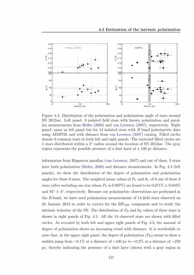
4.3 Estimation of the intrinsic polarization
Figure 4.3: Distribution of the polarization and polarization angle of stars aroundSN 2012aw. Left panel: 9 isolated field stars with known polarization and paral-lax measurements from Heiles (2000) and van Leeuwen (2007), respectively. Rightpanel: same as left panel but for 14 isolated stars with R band polarimetric datausing AIMPOL and with distance from van Leeuwen (2007) catalog. Filled circlesdenote 9 common stars in both left and right panels. The encircled filled circles are5 stars distributed within a 2 radius around the location of SN 2012aw. The grayregion represents the possible presence of a dust layer at a 100 pc distance.
information from Hipparcos parallax (van Leeuwen, 2007) and out of these, 9 stars
have both polarization (Heiles, 2000) and distance measurements. In Fig. 4.3 (left
panels), we show the distribution of the degree of polarization and polarization
angles for these 9 stars. The weighted mean values of PV and θV of 8 out of these 9
stars (after excluding one star whose PV is 0.007%) are found to be 0.071%± 0.010%
and 83 ± 4, respectively. Because our polarimetric observations are performed in
the R-band, we have used polarization measurements of 14 field stars observed on
20 January 2013 in order to correct for the ISPMW component and to study the
intrinsic behavior of the SN. The distribution of PR and θR values of these stars is
shown in right panels of Fig. 4.3. All the 14 observed stars are shown with filled
circles. As revealed by both left and upper right panels of Fig. 4.3, the amount of
degree of polarization shows an increasing trend with distance. It is worthwhile to
note that, in the upper right panel, the degree of polarization (PR) seems to show a
sudden jump from ∼0.1% at a distance of ∼100 pc to ∼0.2% at a distance of ∼250
pc, thereby indicating the presence of a dust layer (shown with a gray region in
121
4. BROAD BAND POLARIMETRIC STUDY OF THE TYPE IIPSN 2012AW
Fig. 4.3) at ∼100 pc. Whereas, the polarization angles of the stars from the Heiles
catalog (left bottom panel) and those observed from the present set-up in R-band
(except few stars) are distributed between 50 − 100 as shown with the dashed
lines (in Fig. 4.3). The Gaussian mean value of θR using the 14 stars is found to be
∼82. This indicates the presence of a uniform dust layer towards the direction of
SN 2012aw, which nearly contributes ∼0.1% to ∼0.2% of polarization and having
a mean magnetic field orientation ∼82. Therefore, we believe that most probably,
the ISPMW component is dominated by the contribution from this dust layer.
To determine the ISPMW component, firstly the PR and θR values of all the
field stars as well as the SN were transformed into the Stokes parameters using the
following relations1:
QR = PR cos 2θR, (4.3)
UR = PR sin 2θR. (4.4)
Then, the weighted mean Stokes parameters were estimated considering (a) all
the 14 field stars distributed over all distances, and (b) only 10 field stars distributed
beyond a distance of 100 pc. These weighted Stokes parameters (<UR>, <QR>)
were converted back to PR and θR using the following relations:
PR =
√
QR2 + UR
2, (4.5)
θR = 0.5× arctan
(
UR
QR
)
. (4.6)
The <UR>, <QR>, <PR> and <θR> values (as estimated following two ways)
are listed in Table 4.3. It is clear from this table that the <PR> of the 14 stars
is relatively smaller than that determined using the 10 stars. This could be due
to the fact that the weighted mean values for stars at all distances may skew the
result towards the brighter and more nearby stars which is likely incorrect. Whereas
the <θR> values in the two cases nearly matches each other and mimic the mean
magnetic field orientation (∼82) of the dust layer as noticed above. To avoid the
values biased towards the lower end due to nearby and brighter stars, we have
1Our polarimeter and software have been designed in such a way that we get P and θ throughfitting the equation 4.1 on four Stokes parameters obtained at four positions of the half-wave plateas mentioned in Section 4.2
122
4.3 Estimation of the intrinsic polarization
considered the polarization measurements of the 10 stars distributed beyond a 100
pc distance to estimate the ISPMW component. In addition, using these 10 stars
which are distributed beyond 100 pc essentially may take care of the contribution
from the dust layer at a distance of 100 pc. Therefore, we consider the <QR>
= − 0.154 ± 0.002%, <UR> = 0.032 ± 0.002% values as the ISPMW component
(i.e. <QISPMW> = <QR> and <UISPMW
> = <UR>). These weighted mean values
have been subtracted vectorially from the Stokes parameters of the SN using the
relations:
Qint = QSN −<QISPMW>, (4.7)
Uint = USN −<UISPMW>, (4.8)
where QSN , USN and Qint , Uint denote respectively the observed and intrinsic
(ISPMW corrected) Stokes parameters of the SN. The resulting intrinsic Stokes pa-
rameters (Qint, Uint) were converted into Pint and θint using the relations 4.5 and
4.6. These intrinsic values for the SN are respectively listed in columns 6 and 7
in Table 4.1 and plotted in Fig. 4.5(a) and (b), with filled circles connected with a
thick line.
The reddening, E(B−V ) due to Milky Way dust in the direction of SN 2012aw,
as derived from the 100-µm all-sky dust extinction map of Schlegel, Finkbeiner
& Davis (1998), was found to be 0.0278 ± 0.0002 mag. According to the mean
polarization efficiency relation Pmean = 5 × E(B − V ) (Serkowski et al., 1975), the
polarization value is estimated to be Pmean ∼0.14% which closely matches with the
weighted mean polarization value, 0.157 ± 0.002% obtained using the 10 fields stars
distributed beyond a 100 pc distance (cf. Table 4.3). It is clear that polarization
values obtained both from the present observations of the field stars and the mean
polarization efficiency relation are similar which implies that the dust grains in the
local interstellar medium (ISM) probably exhibit a mean polarization efficiency.
4.3.2 Interstellar polarization due to the host galactic dust
(ISPHG)
The reddening, E(B−V ), due to dust in the SN 2012aw host galaxy was found to be
0.046 ± 0.008 mag (see Bose et al., 2013). This value was derived using the empirical
correlation, between reddening and the Na I D lines, given by Poznanski et al.
123
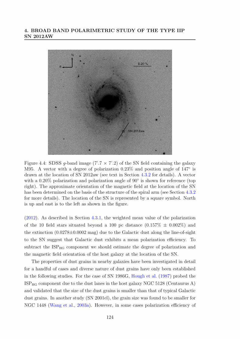
4. BROAD BAND POLARIMETRIC STUDY OF THE TYPE IIPSN 2012AW
Figure 4.4: SDSS g-band image (7’.7 × 7’.2) of the SN field containing the galaxyM95. A vector with a degree of polarization 0.23% and position angle of 147 isdrawn at the location of SN 2012aw (see text in Section 4.3.2 for details). A vectorwith a 0.20% polarization and polarization angle of 90 is shown for reference (topright). The approximate orientation of the magnetic field at the location of the SNhas been determined on the basis of the structure of the spiral arm (see Section 4.3.2for more details). The location of the SN is represented by a square symbol. Northis up and east is to the left as shown in the figure.
(2012). As described in Section 4.3.1, the weighted mean value of the polarization
of the 10 field stars situated beyond a 100 pc distance (0.157% ± 0.002%) and
the extinction (0.0278±0.0002 mag) due to the Galactic dust along the line-of-sight
to the SN suggest that Galactic dust exhibits a mean polarization efficiency. To
subtract the ISPHG component we should estimate the degree of polarization and
the magnetic field orientation of the host galaxy at the location of the SN.
The properties of dust grains in nearby galaxies have been investigated in detail
for a handful of cases and diverse nature of dust grains have only been established
in the following studies. For the case of SN 1986G, Hough et al. (1987) probed the
ISPHG component due to the dust lanes in the host galaxy NGC 5128 (Centaurus A)
and validated that the size of the dust grains is smaller than that of typical Galactic
dust grains. In another study (SN 2001el), the grain size was found to be smaller for
NGC 1448 (Wang et al., 2003a). However, in some cases polarization efficiency of
124
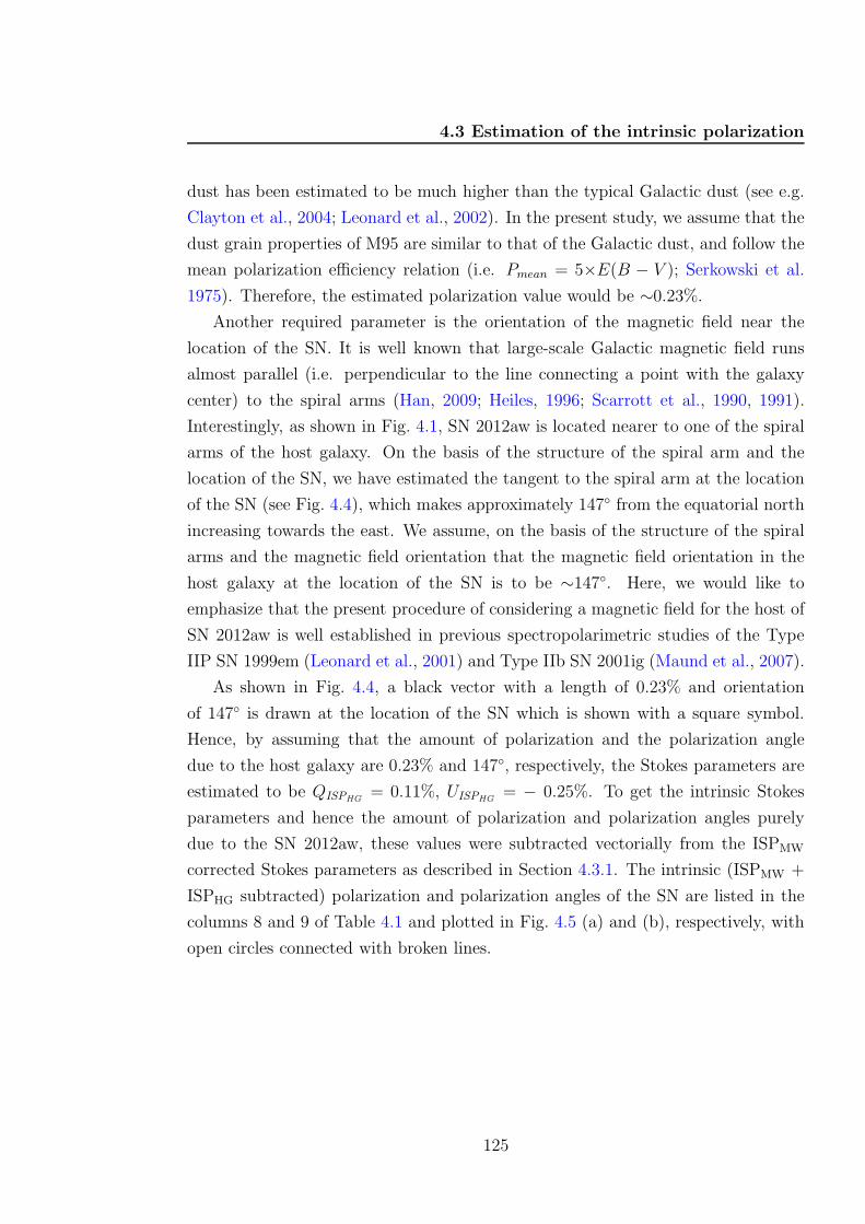
4.3 Estimation of the intrinsic polarization
dust has been estimated to be much higher than the typical Galactic dust (see e.g.
Clayton et al., 2004; Leonard et al., 2002). In the present study, we assume that the
dust grain properties of M95 are similar to that of the Galactic dust, and follow the
mean polarization efficiency relation (i.e. Pmean = 5×E(B − V ); Serkowski et al.
1975). Therefore, the estimated polarization value would be ∼0.23%.
Another required parameter is the orientation of the magnetic field near the
location of the SN. It is well known that large-scale Galactic magnetic field runs
almost parallel (i.e. perpendicular to the line connecting a point with the galaxy
center) to the spiral arms (Han, 2009; Heiles, 1996; Scarrott et al., 1990, 1991).
Interestingly, as shown in Fig. 4.1, SN 2012aw is located nearer to one of the spiral
arms of the host galaxy. On the basis of the structure of the spiral arm and the
location of the SN, we have estimated the tangent to the spiral arm at the location
of the SN (see Fig. 4.4), which makes approximately 147 from the equatorial north
increasing towards the east. We assume, on the basis of the structure of the spiral
arms and the magnetic field orientation that the magnetic field orientation in the
host galaxy at the location of the SN is to be ∼147. Here, we would like to
emphasize that the present procedure of considering a magnetic field for the host of
SN 2012aw is well established in previous spectropolarimetric studies of the Type
IIP SN 1999em (Leonard et al., 2001) and Type IIb SN 2001ig (Maund et al., 2007).
As shown in Fig. 4.4, a black vector with a length of 0.23% and orientation
of 147 is drawn at the location of the SN which is shown with a square symbol.
Hence, by assuming that the amount of polarization and the polarization angle
due to the host galaxy are 0.23% and 147, respectively, the Stokes parameters are
estimated to be QISPHG= 0.11%, UISPHG
= − 0.25%. To get the intrinsic Stokes
parameters and hence the amount of polarization and polarization angles purely
due to the SN 2012aw, these values were subtracted vectorially from the ISPMW
corrected Stokes parameters as described in Section 4.3.1. The intrinsic (ISPMW +
ISPHG subtracted) polarization and polarization angles of the SN are listed in the
columns 8 and 9 of Table 4.1 and plotted in Fig. 4.5 (a) and (b), respectively, with
open circles connected with broken lines.
125
4. BROAD BAND POLARIMETRIC STUDY OF THE TYPE IIPSN 2012AW
Figure 4.5: Panels (a) and (b): Temporal evolution of the polarization and polariza-tion angles of SN 2012aw in R band, respectively. Filled circles connected with thicklines denote the temporal evolution of the polarization and polarization angles aftersubtracting the ISPMW component only, whereas those corrected for both ISPMW +ISPHG components are represented with open circles connected with broken lines.The observed polarization parameters are shown with gray filled circles in panels(a) and (b). The bottom panel (d) shows the calibrated R band LC of SN 2012awobtained with ST (see Bose et al., 2013). The photometric data shown within theshaded region in the bottom panel (d) is re-plotted in panel (c) for a better clarity.
126
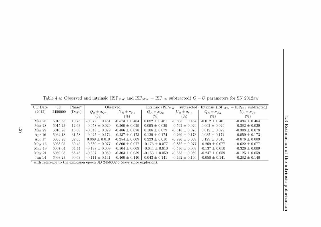
4.3
Estim
atio
nofth
eintrin
sicpolariz
atio
n
Table 4.4: Observed and intrinsic (ISPMW and ISPMW + ISPHG subtracted) Q− U parameters for SN 2012aw.
UT Date JD Phasea Observed Intrinsic (ISPMW subtracted) Intrinsic (ISPMW + ISPHG subtracted)(2012) 2450000 (Days) QR ± σQR
UR ± σURQR ± σQR
UR ± σURQR ± σQR
UR ± σUR
(%) (%) (%) (%) (%) (%)Mar 26 6013.35 10.75 -0.072 ± 0.461 -0.573 ± 0.464 0.082 ± 0.461 -0.605 ± 0.464 -0.012 ± 0.461 -0.394 ± 0.464Mar 28 6015.23 12.63 -0.058 ± 0.029 -0.560 ± 0.029 0.095 ± 0.029 -0.592 ± 0.029 0.002 ± 0.029 -0.382 ± 0.029Mar 29 6016.28 13.68 -0.048 ± 0.079 -0.486 ± 0.078 0.106 ± 0.079 -0.518 ± 0.078 0.012 ± 0.079 -0.308 ± 0.078Apr 16 6034.18 31.58 -0.025 ± 0.174 -0.237 ± 0.173 0.129 ± 0.174 -0.269 ± 0.173 0.035 ± 0.174 -0.059 ± 0.173Apr 17 6035.25 32.65 0.069 ± 0.010 -0.254 ± 0.009 0.223 ± 0.010 -0.286 ± 0.009 0.129 ± 0.010 -0.076 ± 0.009May 15 6063.05 60.45 -0.330 ± 0.077 -0.800 ± 0.077 -0.176 ± 0.077 -0.832 ± 0.077 -0.269 ± 0.077 -0.622 ± 0.077May 19 6067.04 64.44 -0.198 ± 0.009 -0.504 ± 0.009 -0.044 ± 0.010 -0.536 ± 0.009 -0.137 ± 0.010 -0.326 ± 0.009May 21 6069.08 66.48 -0.307 ± 0.059 -0.303 ± 0.059 -0.153 ± 0.059 -0.335 ± 0.059 -0.247 ± 0.059 -0.125 ± 0.059Jun 14 6093.23 90.63 -0.111 ± 0.141 -0.460 ± 0.140 0.043 ± 0.141 -0.492 ± 0.140 -0.050 ± 0.141 -0.282 ± 0.140
a with reference to the explosion epoch JD 2456002.6 (days since explosion).
127
4. BROAD BAND POLARIMETRIC STUDY OF THE TYPE IIPSN 2012AW
4.4 Discussion
4.4.1 Polarization light curve (PLC) analysis
In this section, we analyze the evolution of the PLC and its possible resemblance with
the photometric light curve (LC) of SN 2012aw as shown in Fig 4.5. The calibrated
R-band magnitudes have been taken from Bose et al. (2013) which shows different
evolutionary phases of the LC as described in Falk & Arnett (1977); Grassberg
et al. (1971); Utrobin (2007). Since in the present study, polarimetric data sets are
limited up to the plateau phase, in Fig. 4.5 (panels c and d), only the adiabatic
cooling phase and the phase of cooling and recombination wave are shown.
The temporal variation of the ISPMW corrected degree of polarization (PR) val-
ues (shown with filled circles, Fig. 4.5a) shows a maximum and minimum values of
∼0.9% and ∼0.3%, respectively with a possible trend of variations in accordance
with the R-band LC as shown in panel 4.5(c). Although there is a significant
reduction in ISPMW + ISPHG corrected PR values (open circles, Fig. 4.5a), its re-
semblance with the photometric light curve (panel c) remains similar. However,
both the ISPMW and ISPMW + ISPHG corrected polarization angles (θR, shown with
filled circles in Fig. 4.5(b)) do not show much variation during the similar epochs
of observations and are distributed around a weighted mean value of ∼138. Inter-
estingly, the first (10-14 days) three measurements of ISPMW corrected PR and θR
are almost constant. During this adiabatic cooling phase, the SN LC seems to be
brightened by ∼0.12 magnitude as shown in Fig. 4.5c.
It is worthwhile to note that dips observed around 35 days in the LC of the
SN and in the ISPMW + ISPHG corrected PR are temporally correlated with a
minimum amount of polarization (∼0.07%). This observed feature during the end
of the adiabatic cooling or early recombination phase could be attributed to several
reasons e.g., (i) changes in the geometry i.e., transition from more asphericity to
sphericity of the SN, (ii) modification in the density of scatterers (electrons and/or
ions), (iii) mechanism of scattering i.e., single and (or) multiple scattering, (iv)
changes in the clumpiness of the SN envelope, (v) changes in the electron-scattering
atmosphere of the SN, and (vi) interaction of the SN with a dense circumstellar
medium. In the recombination phase (∼40 days onwards), the evolution in the
values of ISPMW + ISPHG corrected PR and θR are in such a way that the amount
of polarization shows an increasing trend. This increasing trend could suggest that
128
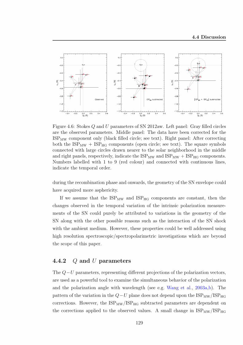
4.4 Discussion
Figure 4.6: Stokes Q and U parameters of SN 2012aw. Left panel: Gray filled circlesare the observed parameters. Middle panel: The data have been corrected for theISPMW component only (black filled circle; see text). Right panel: After correctingboth the ISPMW + ISPHG components (open circle; see text). The square symbolsconnected with large circles drawn nearer to the solar neighborhood in the middleand right panels, respectively, indicate the ISPMW and ISPMW + ISPHG components.Numbers labelled with 1 to 9 (red colour) and connected with continuous lines,indicate the temporal order.
during the recombination phase and onwards, the geometry of the SN envelope could
have acquired more asphericity.
If we assume that the ISPMW and ISPHG components are constant, then the
changes observed in the temporal variation of the intrinsic polarization measure-
ments of the SN could purely be attributed to variations in the geometry of the
SN along with the other possible reasons such as the interaction of the SN shock
with the ambient medium. However, these properties could be well addressed using
high resolution spectroscopic/spectropolarimetric investigations which are beyond
the scope of this paper.
4.4.2 Q and U parameters
The Q−U parameters, representing different projections of the polarization vectors,
are used as a powerful tool to examine the simultaneous behavior of the polarization
and the polarization angle with wavelength (see e.g. Wang et al., 2003a,b). The
pattern of the variation in the Q−U plane does not depend upon the ISPMW/ISPHG
corrections. However, the ISPMW/ISPHG subtracted parameters are dependent on
the corrections applied to the observed values. A small change in ISPMW/ISPHG
129
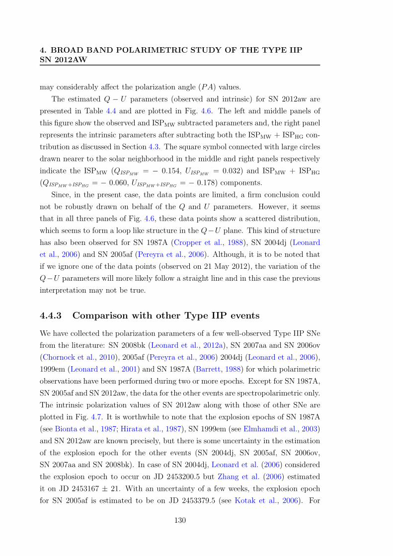
4. BROAD BAND POLARIMETRIC STUDY OF THE TYPE IIPSN 2012AW
may considerably affect the polarization angle (PA) values.
The estimated Q − U parameters (observed and intrinsic) for SN 2012aw are
presented in Table 4.4 and are plotted in Fig. 4.6. The left and middle panels of
this figure show the observed and ISPMW subtracted parameters and, the right panel
represents the intrinsic parameters after subtracting both the ISPMW + ISPHG con-
tribution as discussed in Section 4.3. The square symbol connected with large circles
drawn nearer to the solar neighborhood in the middle and right panels respectively
indicate the ISPMW (QISPMW= − 0.154, UISPMW
= 0.032) and ISPMW + ISPHG
(QISPMW +ISPHG= − 0.060, UISPMW+ISPHG
= − 0.178) components.
Since, in the present case, the data points are limited, a firm conclusion could
not be robustly drawn on behalf of the Q and U parameters. However, it seems
that in all three panels of Fig. 4.6, these data points show a scattered distribution,
which seems to form a loop like structure in the Q−U plane. This kind of structure
has also been observed for SN 1987A (Cropper et al., 1988), SN 2004dj (Leonard
et al., 2006) and SN 2005af (Pereyra et al., 2006). Although, it is to be noted that
if we ignore one of the data points (observed on 21 May 2012), the variation of the
Q−U parameters will more likely follow a straight line and in this case the previous
interpretation may not be true.
4.4.3 Comparison with other Type IIP events
We have collected the polarization parameters of a few well-observed Type IIP SNe
from the literature: SN 2008bk (Leonard et al., 2012a), SN 2007aa and SN 2006ov
(Chornock et al., 2010), 2005af (Pereyra et al., 2006) 2004dj (Leonard et al., 2006),
1999em (Leonard et al., 2001) and SN 1987A (Barrett, 1988) for which polarimetric
observations have been performed during two or more epochs. Except for SN 1987A,
SN 2005af and SN 2012aw, the data for the other events are spectropolarimetric only.
The intrinsic polarization values of SN 2012aw along with those of other SNe are
plotted in Fig. 4.7. It is worthwhile to note that the explosion epochs of SN 1987A
(see Bionta et al., 1987; Hirata et al., 1987), SN 1999em (see Elmhamdi et al., 2003)
and SN 2012aw are known precisely, but there is some uncertainty in the estimation
of the explosion epoch for the other events (SN 2004dj, SN 2005af, SN 2006ov,
SN 2007aa and SN 2008bk). In case of SN 2004dj, Leonard et al. (2006) considered
the explosion epoch to occur on JD 2453200.5 but Zhang et al. (2006) estimated
it on JD 2453167 ± 21. With an uncertainty of a few weeks, the explosion epoch
for SN 2005af is estimated to be on JD 2453379.5 (see Kotak et al., 2006). For
130
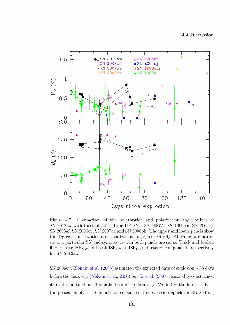
4.4 Discussion
Figure 4.7: Comparison of the polarization and polarization angle values ofSN 2012aw with those of other Type IIP SNe: SN 1987A, SN 1999em, SN 2004dj,SN 2005af, SN 2006ov, SN 2007aa and SN 2008bk. The upper and lower panels showthe degree of polarization and polarization angle, respectively. All values are intrin-sic to a particular SN and symbols used in both panels are same. Thick and brokenlines denote ISPMW and both ISPMW + ISPHG subtracted components, respectivelyfor SN 2012aw.
SN 2006ov, Blondin et al. (2006) estimated the expected date of explosion ∼36 days
before the discovery (Nakano et al., 2006) but Li et al. (2007) reasonably constrained
its explosion to about 3 months before the discovery. We follow the later study in
the present analysis. Similarly we considered the explosion epoch for SN 2007aa,
131
4. BROAD BAND POLARIMETRIC STUDY OF THE TYPE IIPSN 2012AW
∼20 days before the discovery (see Doi et al., 2007; Folatelli et al., 2007) and for
SN 2008bk, JD 2454550 (2008 March 24) has been considered as the explosion epoch
(see Morrell & Stritzinger, 2008; Van Dyk et al., 2010).
Shifting the phase (days after the explosion) by 21 days, the evolution of the
degree of polarization of SN 2004dj is very much similar to what has been seen
for SN 2012aw as shown in Fig. 4.7. However, it is important to mention that
for SN 2004dj the degree of polarization increased after the end of the plateau
phase (when we see through the H-rich shell); whereas for SN 2012aw, the degree
of polarization increased (around 60 days) during the plateau phase which could be
a possible indication of a diverse nature of the two events. However, it is noticeable
that like for SN 2008bk, SN 2012aw is also strongly polarized well before the end
of the plateau (see Leonard et al., 2012a), indicating a possible similarity for both
these events. In the early phase (∼10 − 30 days), the ISPMW corrected PLC of
SN 2012aw matched that of SN 1987A, whereas in the later phase (∼30 − 45 days)
it closely matched that of SN 2005af. Nonetheless, it is worthwhile to mention that
in order to derive the polarization parameters of SN 1987A and SN 2005af, the
ISPHG components were not subtracted in the respective studies. The polarimetric
observations of SN 1999em are sparse; the polarization levels at different epochs seem
to match the ISPMW + ISPHG corrected PLC of SN 2012aw. It is also obvious from
Fig. 4.7 that the polarization values of SN 2006ov remained more than 1% during all
three epochs of observation which is higher than that of any of the Type IIP events
in the list. Fig. 4.7 gives an important information regarding the evolution of the
ejecta for similar types of SNe. By comparing the PLCs of various IIP SNe shown
with different symbols in Fig. 4.7 (filled star: SN 1987A, filled triangle: SN 1999em,
filled square: SN 2004dj, open star: SN 2005af, open triangle: SN 2006ov, cross:
SN 2007aa, open square: SN 2008bk and for SN 2012aw symbols are the same as
in Fig. 4.5), it could be conjectured that the properties of the ejecta from Type IIP
SNe are diverse in nature as noticed by Chornock et al. (2010).
We have also compared the ISPMW and ISPHG corrected PLCs of SN 2012aw with
those of other Type Ib/c CCSNe. Type Ib/c SNe are naturally more asymmetric in
comparison to Type IIP SNe because they lack a thick He blanket that smears out
the internal geometry. Therefore, a higher degree of polarization is observed in case
of Type Ib/c SNe. In the present analysis, the PLC of SN 2012aw is also clearly
showing a lower degree of polarization in comparison to various well studied Type
Ib/c CCSNe (e.g. SN 2007uy, SN 2008D; Gorosabel et al., 2010). However, it is
132
4.5 Conclusions
important to note that the PR peak value for SN 2012aw seen at ∼60 days is slightly
less than the intrinsic polarization value of ∼1% for Type Ic SN 2008D which was
related to a violent X-ray transient (see Gorosabel et al., 2010). Here it is noticeable
that present PLC interpretations of SN 2012aw depend a lot on a single data point
(May 15) which is significantly higher in the percentage polarization than the data
taken at other epochs.
4.5 Conclusions
We have presented results based on 9 epoch R band imaging polarimetric observa-
tions of Type IIP supernova SN 2012aw. To the best of our knowledge, the initial
three epoch polarimetric observations presented here are the earliest optical polari-
metric data reported for this event. It was not possible to monitor the SN during
the beginning of the nebular or post-nebular phase due to observational constraintsi.
However present observations cover almost up to the end of the plateau phase (∼90
days). The main results of our present study are the following:
• The observed broad-band polarization for the initial three epochs is ∼0.6%,
then decreases down to ∼0.3% following a sudden increase up to ∼0.9% on 15
may 2013 and at later epochs it seems to show a declining trend. However,
the observed polarization angle is almost constant, superimposed with slight
variations.
• To study the intrinsic polarization properties of SN 2012aw, we subtracted
the contribution due to ISPMW and ISPHG from the observed P and θ values
of the SN. The ISPMW component was determined using the polarimetric
observations of 10 field stars distributed within a 10 radius around the SN
and located beyond a 100 pc distance. The estimated Stokes parameters of
ISPMW are found to be <QISPMW> = − 0.154 ± 0.002% and <UISPMW
> =
0.032 ± 0.002% (equivalent to <PISPMW> = 0.157 ± 0.002 and <θISPMW
> =
84.10 ± 0.56). We also estimated the degree of polarization (0.23%) and
polarization angle (147) at the location of the SN by using the extinction
value from the Schlegel map assuming that the host galactic dust follows the
mean polarization efficiency and that the magnetic field in the host galaxy
follows the structure of the spiral arms.
133
4. BROAD BAND POLARIMETRIC STUDY OF THE TYPE IIPSN 2012AW
• The intrinsic polarization parameters of SN 2012aw follow trends of the pho-
tometric LC which could be attributed to the small scale variations in the SN
atmosphere or their interaction with the ambient medium.
• Polarimetric parameters of this SN are compared with other well studied Type
IIP events. During the early phase (∼10 − 30 days), the ISPMW subtracted
PLC of SN 2012aw matches that of SN 1987A whereas at later epochs (∼30
− 45 days) it matches that of SN 2005af.
134
Part III
The 4m International Liquid
Mirror Telescope and search for
supernovae
135

Chapter 5
The 4m International Liquid
Mirror Telescope project
5.1 Introduction
Presently, the Large Zenithal Telescope (LZT) is the largest working LMT (see
Sect. 1.3.4 for other LMTs). But the conditions are not optimal in order to carry
out astronomical observations. The site has average seeing of ∼2.2” and average
30% clear sky (Hickson et al., 2007). These numbers are not encouraging in terms
of astronomical efficiency. Therefore, a full time LMT project entirely dedicated to
astronomical observations was proposed and the idea of building an International
Liquid Mirror Telescope (ILMT1) was born. During the last recent years, several
experiments have been performed and the telescope is now ready for installation.
First light is expected in the year 2015.
The ILMT project is a scientific collaboration between four countries: Belgium,
India, Canada and Poland. The main participating institutions are: Liege Institute
of Astrophysics and Geophysics (University of Liege, Belgium), the Royal Obser-
vatory of Belgium, the Aryabhatta Research Institute of Observational Sciences
(ARIES, Nainital, India), the Observatory of Poznan (Poland) and several Cana-
dian universities (British Columbia, Laval, Montreal, Toronto, Victoria and York).
The AMOS (Advanced Mechanical and Optical Systems) company in Belgium has
participated to the fabrication of the telescope.
It should be noted that the working principles of LZT and ILMT are the same
but there are some technical differences as listed in Table 5.1.
1more details about the ILMT can be found at http://www.aeos.ulg.ac.be/LMT
137
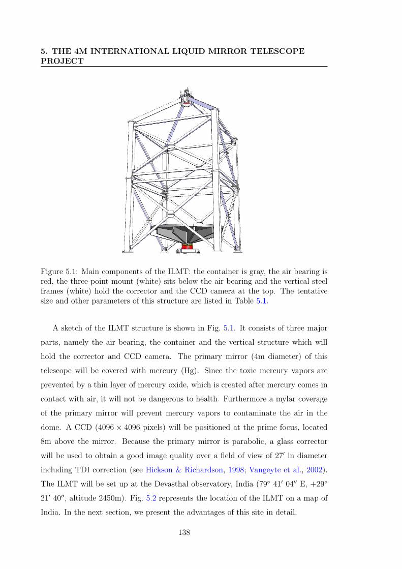
5. THE 4M INTERNATIONAL LIQUID MIRROR TELESCOPEPROJECT
Figure 5.1: Main components of the ILMT: the container is gray, the air bearing isred, the three-point mount (white) sits below the air bearing and the vertical steelframes (white) hold the corrector and the CCD camera at the top. The tentativesize and other parameters of this structure are listed in Table 5.1.
A sketch of the ILMT structure is shown in Fig. 5.1. It consists of three major
parts, namely the air bearing, the container and the vertical structure which will
hold the corrector and CCD camera. The primary mirror (4m diameter) of this
telescope will be covered with mercury (Hg). Since the toxic mercury vapors are
prevented by a thin layer of mercury oxide, which is created after mercury comes in
contact with air, it will not be dangerous to health. Furthermore a mylar coverage
of the primary mirror will prevent mercury vapors to contaminate the air in the
dome. A CCD (4096 × 4096 pixels) will be positioned at the prime focus, located
8m above the mirror. Because the primary mirror is parabolic, a glass corrector
will be used to obtain a good image quality over a field of view of 27′ in diameter
including TDI correction (see Hickson & Richardson, 1998; Vangeyte et al., 2002).
The ILMT will be set up at the Devasthal observatory, India (79 41′ 04′′ E, +29
21′ 40′′, altitude 2450m). Fig. 5.2 represents the location of the ILMT on a map of
India. In the next section, we present the advantages of this site in detail.
138
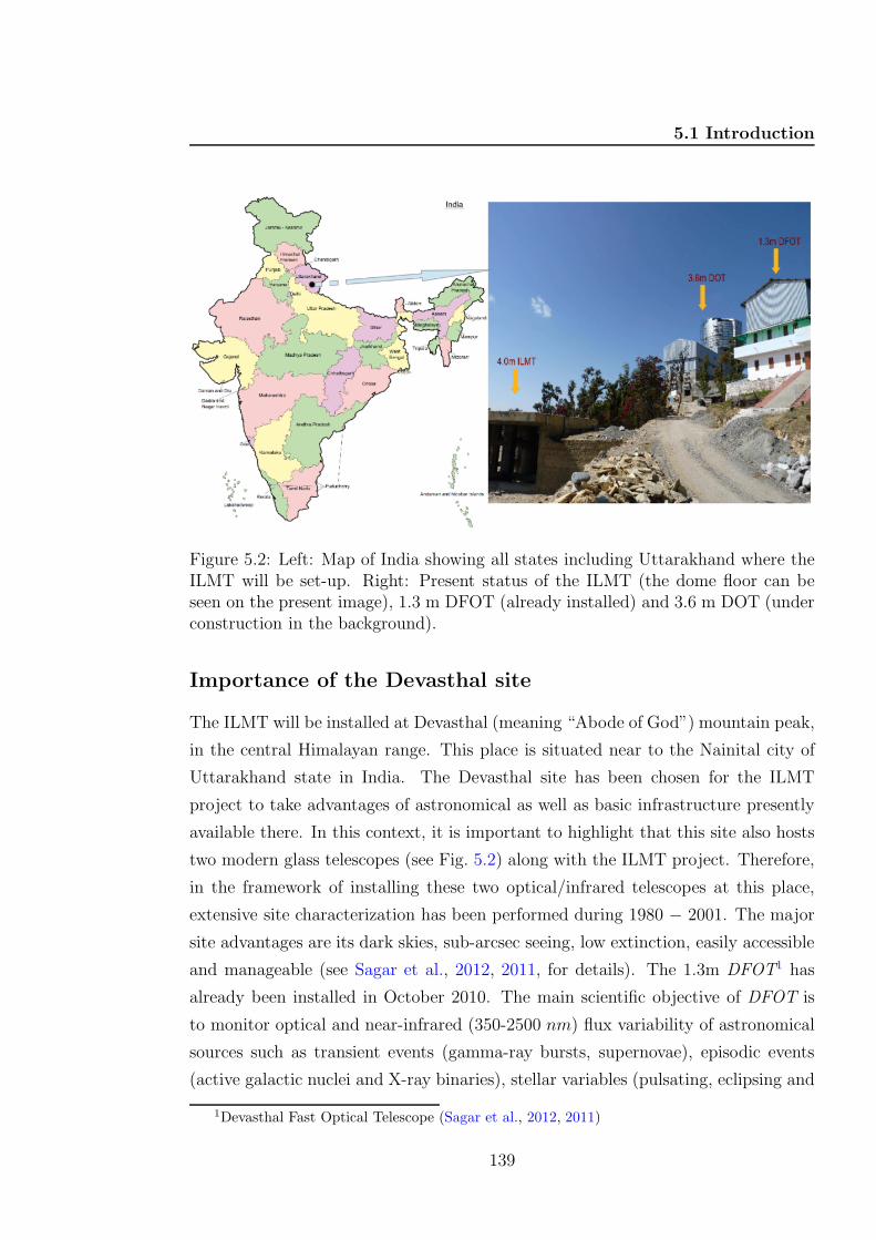
5.1 Introduction
Figure 5.2: Left: Map of India showing all states including Uttarakhand where theILMT will be set-up. Right: Present status of the ILMT (the dome floor can beseen on the present image), 1.3 m DFOT (already installed) and 3.6 m DOT (underconstruction in the background).
Importance of the Devasthal site
The ILMT will be installed at Devasthal (meaning “Abode of God”) mountain peak,
in the central Himalayan range. This place is situated near to the Nainital city of
Uttarakhand state in India. The Devasthal site has been chosen for the ILMT
project to take advantages of astronomical as well as basic infrastructure presently
available there. In this context, it is important to highlight that this site also hosts
two modern glass telescopes (see Fig. 5.2) along with the ILMT project. Therefore,
in the framework of installing these two optical/infrared telescopes at this place,
extensive site characterization has been performed during 1980 − 2001. The major
site advantages are its dark skies, sub-arcsec seeing, low extinction, easily accessible
and manageable (see Sagar et al., 2012, 2011, for details). The 1.3m DFOT1 has
already been installed in October 2010. The main scientific objective of DFOT is
to monitor optical and near-infrared (350-2500 nm) flux variability of astronomical
sources such as transient events (gamma-ray bursts, supernovae), episodic events
(active galactic nuclei and X-ray binaries), stellar variables (pulsating, eclipsing and
1Devasthal Fast Optical Telescope (Sagar et al., 2012, 2011)
139
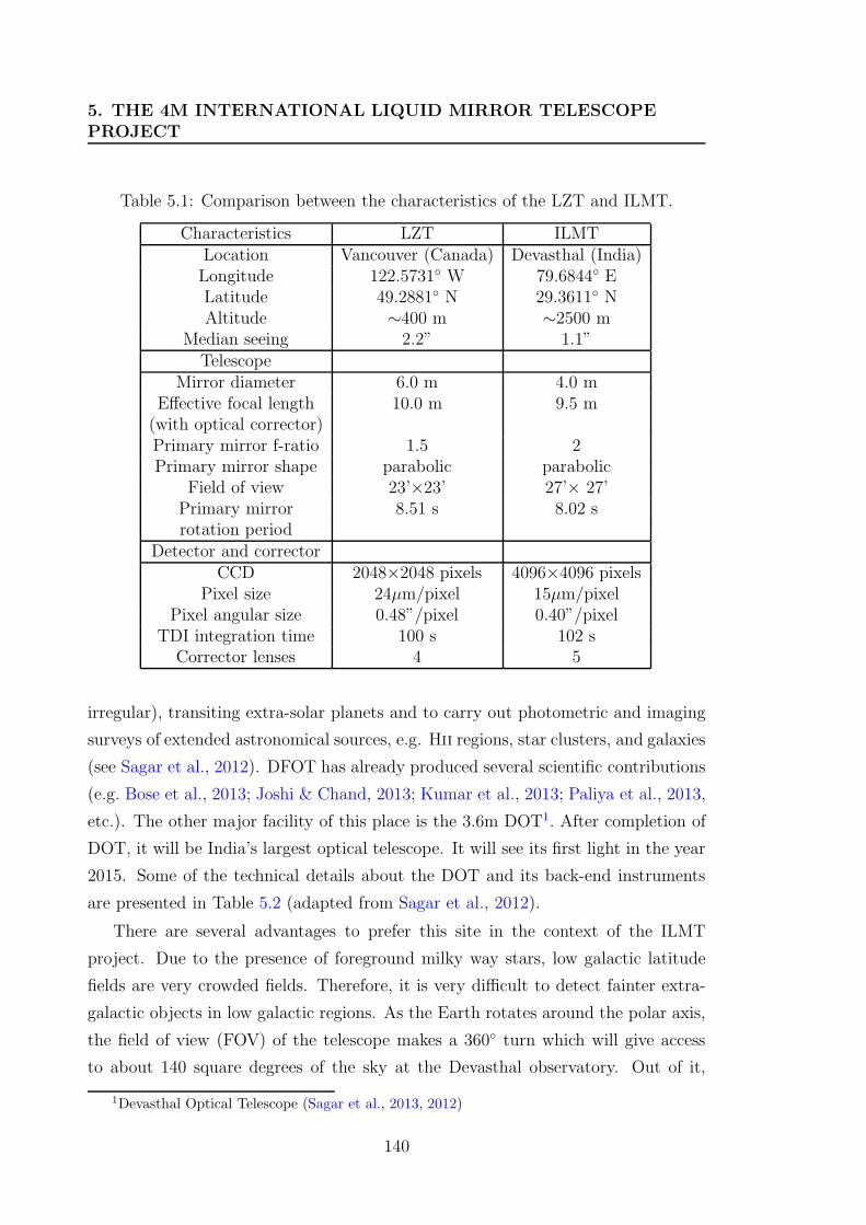
5. THE 4M INTERNATIONAL LIQUID MIRROR TELESCOPEPROJECT
Table 5.1: Comparison between the characteristics of the LZT and ILMT.
Characteristics LZT ILMTLocation Vancouver (Canada) Devasthal (India)Longitude 122.5731 W 79.6844 ELatitude 49.2881 N 29.3611 NAltitude ∼400 m ∼2500 m
Median seeing 2.2” 1.1”Telescope
Mirror diameter 6.0 m 4.0 mEffective focal length 10.0 m 9.5 m(with optical corrector)Primary mirror f-ratio 1.5 2Primary mirror shape parabolic parabolic
Field of view 23’×23’ 27’× 27’Primary mirror 8.51 s 8.02 srotation period
Detector and correctorCCD 2048×2048 pixels 4096×4096 pixels
Pixel size 24µm/pixel 15µm/pixelPixel angular size 0.48”/pixel 0.40”/pixel
TDI integration time 100 s 102 sCorrector lenses 4 5
irregular), transiting extra-solar planets and to carry out photometric and imaging
surveys of extended astronomical sources, e.g. Hii regions, star clusters, and galaxies
(see Sagar et al., 2012). DFOT has already produced several scientific contributions
(e.g. Bose et al., 2013; Joshi & Chand, 2013; Kumar et al., 2013; Paliya et al., 2013,
etc.). The other major facility of this place is the 3.6m DOT1. After completion of
DOT, it will be India’s largest optical telescope. It will see its first light in the year
2015. Some of the technical details about the DOT and its back-end instruments
are presented in Table 5.2 (adapted from Sagar et al., 2012).
There are several advantages to prefer this site in the context of the ILMT
project. Due to the presence of foreground milky way stars, low galactic latitude
fields are very crowded fields. Therefore, it is very difficult to detect fainter extra-
galactic objects in low galactic regions. As the Earth rotates around the polar axis,
the field of view (FOV) of the telescope makes a 360 turn which will give access
to about 140 square degrees of the sky at the Devasthal observatory. Out of it,
1Devasthal Optical Telescope (Sagar et al., 2013, 2012)
140
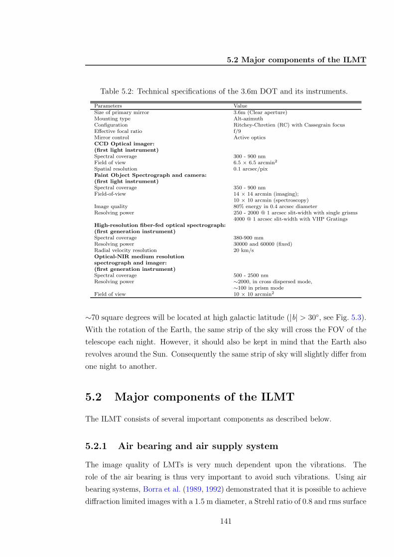
5.2 Major components of the ILMT
Table 5.2: Technical specifications of the 3.6m DOT and its instruments.
Parameters ValueSize of primary mirror 3.6m (Clear aperture)Mounting type Alt-azimuthConfiguration Ritchey-Chretien (RC) with Cassegrain focusEffective focal ratio f/9Mirror control Active opticsCCD Optical imager:(first light instrument)Spectral coverage 300 - 900 nmField of view 6.5 × 6.5 arcmin2
Spatial resolution 0.1 arcsec/pixFaint Object Spectrograph and camera:(first light instrument)Spectral coverage 350 - 900 nmField-of-view 14 × 14 arcmin (imaging);
10 × 10 arcmin (spectroscopy)Image quality 80% energy in 0.4 arcsec diameterResolving power 250 - 2000 @ 1 arcsec slit-width with single grisms
4000 @ 1 arcsec slit-width with VHP GratingsHigh-resolution fiber-fed optical spectrograph:(first generation instrument)Spectral coverage 380-900 mmResolving power 30000 and 60000 (fixed)Radial velocity resolution 20 km/sOptical-NIR medium resolutionspectrograph and imager:(first generation instrument)Spectral coverage 500 - 2500 nmResolving power ∼2000, in cross dispersed mode,
∼100 in prism modeField of view 10 × 10 arcmin2
∼70 square degrees will be located at high galactic latitude (|b| > 30, see Fig. 5.3).
With the rotation of the Earth, the same strip of the sky will cross the FOV of the
telescope each night. However, it should also be kept in mind that the Earth also
revolves around the Sun. Consequently the same strip of sky will slightly differ from
one night to another.
5.2 Major components of the ILMT
The ILMT consists of several important components as described below.
5.2.1 Air bearing and air supply system
The image quality of LMTs is very much dependent upon the vibrations. The
role of the air bearing is thus very important to avoid such vibrations. Using air
bearing systems, Borra et al. (1989, 1992) demonstrated that it is possible to achieve
diffraction limited images with a 1.5 m diameter, a Strehl ratio of 0.8 and rms surface
141
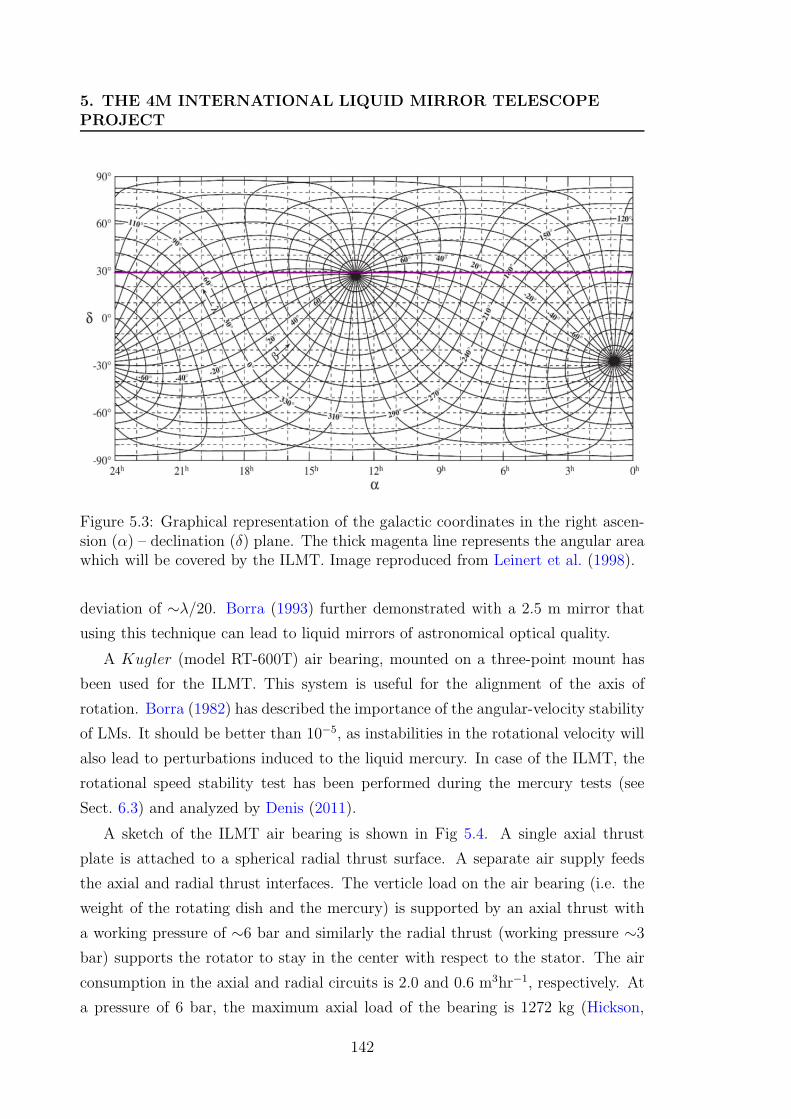
5. THE 4M INTERNATIONAL LIQUID MIRROR TELESCOPEPROJECT
Figure 5.3: Graphical representation of the galactic coordinates in the right ascen-sion (α) – declination (δ) plane. The thick magenta line represents the angular areawhich will be covered by the ILMT. Image reproduced from Leinert et al. (1998).
deviation of ∼λ/20. Borra (1993) further demonstrated with a 2.5 m mirror that
using this technique can lead to liquid mirrors of astronomical optical quality.
A Kugler (model RT-600T) air bearing, mounted on a three-point mount has
been used for the ILMT. This system is useful for the alignment of the axis of
rotation. Borra (1982) has described the importance of the angular-velocity stability
of LMs. It should be better than 10−5, as instabilities in the rotational velocity will
also lead to perturbations induced to the liquid mercury. In case of the ILMT, the
rotational speed stability test has been performed during the mercury tests (see
Sect. 6.3) and analyzed by Denis (2011).
A sketch of the ILMT air bearing is shown in Fig 5.4. A single axial thrust
plate is attached to a spherical radial thrust surface. A separate air supply feeds
the axial and radial thrust interfaces. The verticle load on the air bearing (i.e. the
weight of the rotating dish and the mercury) is supported by an axial thrust with
a working pressure of ∼6 bar and similarly the radial thrust (working pressure ∼3
bar) supports the rotator to stay in the center with respect to the stator. The air
consumption in the axial and radial circuits is 2.0 and 0.6 m3hr−1, respectively. At
a pressure of 6 bar, the maximum axial load of the bearing is 1272 kg (Hickson,
142
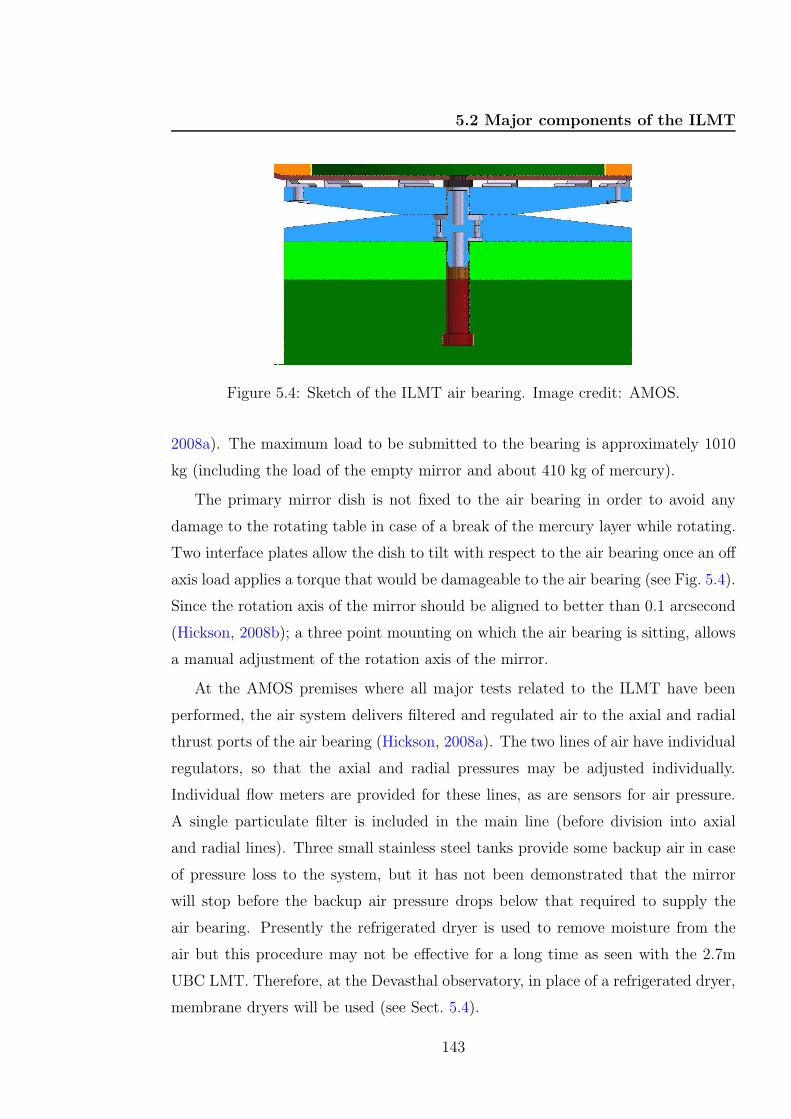
5.2 Major components of the ILMT
Figure 5.4: Sketch of the ILMT air bearing. Image credit: AMOS.
2008a). The maximum load to be submitted to the bearing is approximately 1010
kg (including the load of the empty mirror and about 410 kg of mercury).
The primary mirror dish is not fixed to the air bearing in order to avoid any
damage to the rotating table in case of a break of the mercury layer while rotating.
Two interface plates allow the dish to tilt with respect to the air bearing once an off
axis load applies a torque that would be damageable to the air bearing (see Fig. 5.4).
Since the rotation axis of the mirror should be aligned to better than 0.1 arcsecond
(Hickson, 2008b); a three point mounting on which the air bearing is sitting, allows
a manual adjustment of the rotation axis of the mirror.
At the AMOS premises where all major tests related to the ILMT have been
performed, the air system delivers filtered and regulated air to the axial and radial
thrust ports of the air bearing (Hickson, 2008a). The two lines of air have individual
regulators, so that the axial and radial pressures may be adjusted individually.
Individual flow meters are provided for these lines, as are sensors for air pressure.
A single particulate filter is included in the main line (before division into axial
and radial lines). Three small stainless steel tanks provide some backup air in case
of pressure loss to the system, but it has not been demonstrated that the mirror
will stop before the backup air pressure drops below that required to supply the
air bearing. Presently the refrigerated dryer is used to remove moisture from the
air but this procedure may not be effective for a long time as seen with the 2.7m
UBC LMT. Therefore, at the Devasthal observatory, in place of a refrigerated dryer,
membrane dryers will be used (see Sect. 5.4).
143
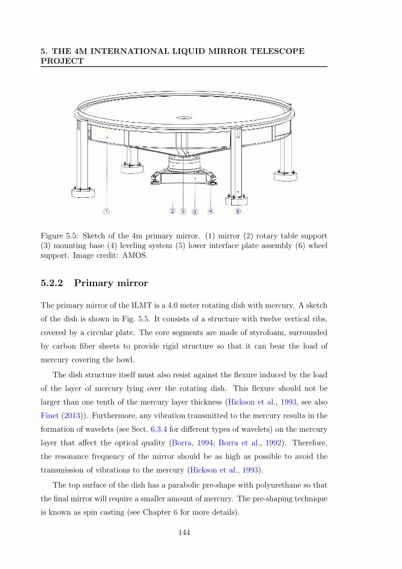
5. THE 4M INTERNATIONAL LIQUID MIRROR TELESCOPEPROJECT
Figure 5.5: Sketch of the 4m primary mirror. (1) mirror (2) rotary table support(3) mounting base (4) leveling system (5) lower interface plate assembly (6) wheelsupport. Image credit: AMOS.
5.2.2 Primary mirror
The primary mirror of the ILMT is a 4.0 meter rotating dish with mercury. A sketch
of the dish is shown in Fig. 5.5. It consists of a structure with twelve vertical ribs,
covered by a circular plate. The core segments are made of styrofoam, surrounded
by carbon fiber sheets to provide rigid structure so that it can bear the load of
mercury covering the bowl.
The dish structure itself must also resist against the flexure induced by the load
of the layer of mercury lying over the rotating dish. This flexure should not be
larger than one tenth of the mercury layer thickness (Hickson et al., 1993, see also
Finet (2013)). Furthermore, any vibration transmitted to the mercury results in the
formation of wavelets (see Sect. 6.3.4 for different types of wavelets) on the mercury
layer that affect the optical quality (Borra, 1994; Borra et al., 1992). Therefore,
the resonance frequency of the mirror should be as high as possible to avoid the
transmission of vibrations to the mercury (Hickson et al., 1993).
The top surface of the dish has a parabolic pre-shape with polyurethane so that
the final mirror will require a smaller amount of mercury. The pre-shaping technique
is known as spin casting (see Chapter 6 for more details).
144
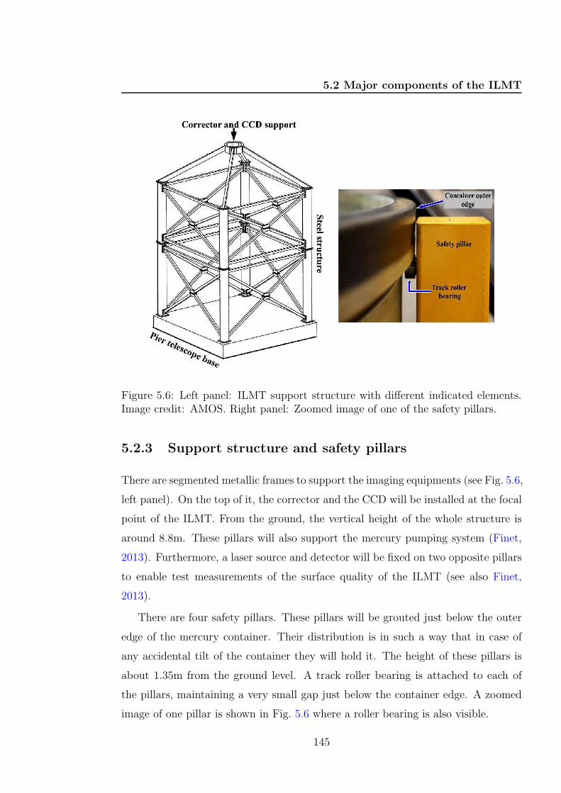
5.2 Major components of the ILMT
Figure 5.6: Left panel: ILMT support structure with different indicated elements.Image credit: AMOS. Right panel: Zoomed image of one of the safety pillars.
5.2.3 Support structure and safety pillars
There are segmented metallic frames to support the imaging equipments (see Fig. 5.6,
left panel). On the top of it, the corrector and the CCD will be installed at the focal
point of the ILMT. From the ground, the vertical height of the whole structure is
around 8.8m. These pillars will also support the mercury pumping system (Finet,
2013). Furthermore, a laser source and detector will be fixed on two opposite pillars
to enable test measurements of the surface quality of the ILMT (see also Finet,
2013).
There are four safety pillars. These pillars will be grouted just below the outer
edge of the mercury container. Their distribution is in such a way that in case of
any accidental tilt of the container they will hold it. The height of these pillars is
about 1.35m from the ground level. A track roller bearing is attached to each of
the pillars, maintaining a very small gap just below the container edge. A zoomed
image of one pillar is shown in Fig. 5.6 where a roller bearing is also visible.
145
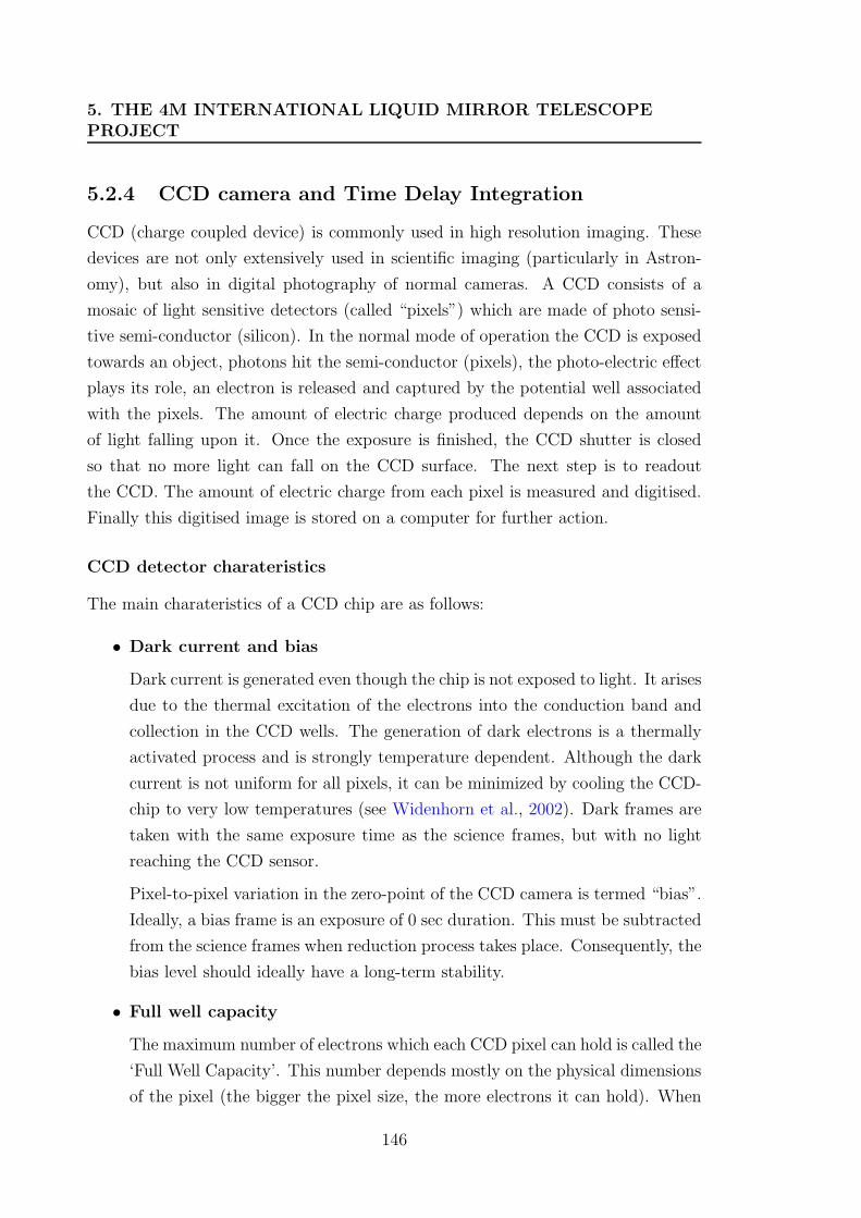
5. THE 4M INTERNATIONAL LIQUID MIRROR TELESCOPEPROJECT
5.2.4 CCD camera and Time Delay Integration
CCD (charge coupled device) is commonly used in high resolution imaging. These
devices are not only extensively used in scientific imaging (particularly in Astron-
omy), but also in digital photography of normal cameras. A CCD consists of a
mosaic of light sensitive detectors (called “pixels”) which are made of photo sensi-
tive semi-conductor (silicon). In the normal mode of operation the CCD is exposed
towards an object, photons hit the semi-conductor (pixels), the photo-electric effect
plays its role, an electron is released and captured by the potential well associated
with the pixels. The amount of electric charge produced depends on the amount
of light falling upon it. Once the exposure is finished, the CCD shutter is closed
so that no more light can fall on the CCD surface. The next step is to readout
the CCD. The amount of electric charge from each pixel is measured and digitised.
Finally this digitised image is stored on a computer for further action.
CCD detector charateristics
The main charateristics of a CCD chip are as follows:
• Dark current and bias
Dark current is generated even though the chip is not exposed to light. It arises
due to the thermal excitation of the electrons into the conduction band and
collection in the CCD wells. The generation of dark electrons is a thermally
activated process and is strongly temperature dependent. Although the dark
current is not uniform for all pixels, it can be minimized by cooling the CCD-
chip to very low temperatures (see Widenhorn et al., 2002). Dark frames are
taken with the same exposure time as the science frames, but with no light
reaching the CCD sensor.
Pixel-to-pixel variation in the zero-point of the CCD camera is termed “bias”.
Ideally, a bias frame is an exposure of 0 sec duration. This must be subtracted
from the science frames when reduction process takes place. Consequently, the
bias level should ideally have a long-term stability.
• Full well capacity
The maximum number of electrons which each CCD pixel can hold is called the
‘Full Well Capacity’. This number depends mostly on the physical dimensions
of the pixel (the bigger the pixel size, the more electrons it can hold). When
146
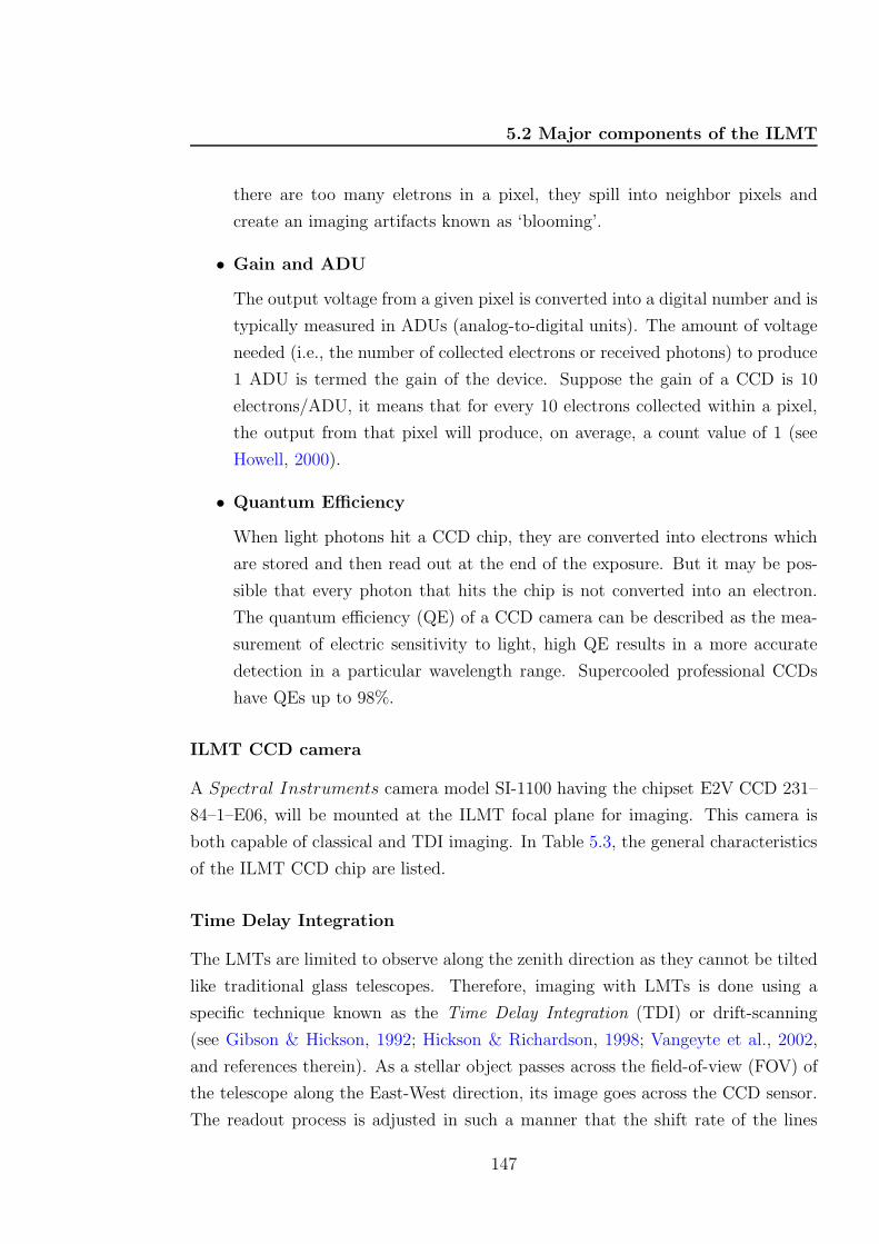
5.2 Major components of the ILMT
there are too many eletrons in a pixel, they spill into neighbor pixels and
create an imaging artifacts known as ‘blooming’.
• Gain and ADU
The output voltage from a given pixel is converted into a digital number and is
typically measured in ADUs (analog-to-digital units). The amount of voltage
needed (i.e., the number of collected electrons or received photons) to produce
1 ADU is termed the gain of the device. Suppose the gain of a CCD is 10
electrons/ADU, it means that for every 10 electrons collected within a pixel,
the output from that pixel will produce, on average, a count value of 1 (see
Howell, 2000).
• Quantum Efficiency
When light photons hit a CCD chip, they are converted into electrons which
are stored and then read out at the end of the exposure. But it may be pos-
sible that every photon that hits the chip is not converted into an electron.
The quantum efficiency (QE) of a CCD camera can be described as the mea-
surement of electric sensitivity to light, high QE results in a more accurate
detection in a particular wavelength range. Supercooled professional CCDs
have QEs up to 98%.
ILMT CCD camera
A Spectral Instruments camera model SI-1100 having the chipset E2V CCD 231–
84–1–E06, will be mounted at the ILMT focal plane for imaging. This camera is
both capable of classical and TDI imaging. In Table 5.3, the general characteristics
of the ILMT CCD chip are listed.
Time Delay Integration
The LMTs are limited to observe along the zenith direction as they cannot be tilted
like traditional glass telescopes. Therefore, imaging with LMTs is done using a
specific technique known as the Time Delay Integration (TDI) or drift-scanning
(see Gibson & Hickson, 1992; Hickson & Richardson, 1998; Vangeyte et al., 2002,
and references therein). As a stellar object passes across the field-of-view (FOV) of
the telescope along the East-West direction, its image goes across the CCD sensor.
The readout process is adjusted in such a manner that the shift rate of the lines
147
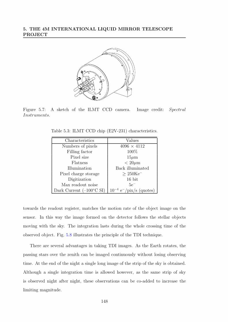
5. THE 4M INTERNATIONAL LIQUID MIRROR TELESCOPEPROJECT
Figure 5.7: A sketch of the ILMT CCD camera. Image credit: SpectralInstruments.
Table 5.3: ILMT CCD chip (E2V-231) characteristics.
Characteristics ValuesNumbers of pixels 4096 × 4112
Filling factor 100%Pixel size 15µmFlatness < 20µm
Illumination Back illuminatedPixel charge storage ≥ 250Ke−
Digitization 16 bitMax readout noise 5e−
Dark Current (–100C SI) 10−4 e−/pix/s (quotes)
towards the readout register, matches the motion rate of the object image on the
sensor. In this way the image formed on the detector follows the stellar objects
moving with the sky. The integration lasts during the whole crossing time of the
observed object. Fig. 5.8 illustrates the principle of the TDI technique.
There are several advantages in taking TDI images. As the Earth rotates, the
passing stars over the zenith can be imaged continuously without losing observing
time. At the end of the night a single long image of the strip of the sky is obtained.
Although a single integration time is allowed however, as the same strip of sky
is observed night after night, these observations can be co-added to increase the
limiting magnitude.
148
5.2 Major components of the ILMT
Figure 5.8: Illustration of TDI imaging.
5.2.5 Filters
The ILMT filter system comprises g′, r′ and i′ which is based on the SDSS photo-
metric system. These filters cover the optical and near infrared wavelength range.
The adopted filters were prefered in order to directly compare the data produced
by the ILMT with those from other large surveys e.g. SDSS, CFHT, etc. It should
be mentioned that the SDSS has a slightly different photometric system (u, g, r, i, z
bands instead of u′, g′, r′, i′, z′) therefore, a straightforward colour transformation
will be peformed (for example, see http://classic.sdss.org/dr4/algorithms/
jeg_photometric_eq_dr1.html#usno2SDSS).
The telescope will mostly operate in the i′ filter dedicated to the time variability
survey. In addition, observations during a larger number of nights will be possible
with the i′ filter because this spectral range is less sensitive to the bright phases
of the moon. Imaging in g′ and r′ will be performed in order to ensure a correct
photometric calibration and rough characterization of all the detected objects. A
few characteristics of the g′, r′, and i′ filters are summarized in Table 5.4.
149
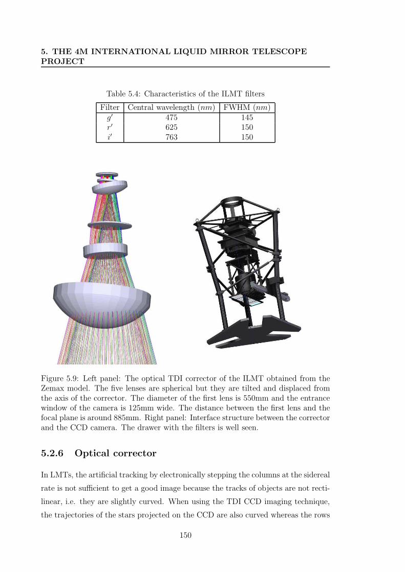
5. THE 4M INTERNATIONAL LIQUID MIRROR TELESCOPEPROJECT
Table 5.4: Characteristics of the ILMT filters
Filter Central wavelength (nm) FWHM (nm)g′ 475 145r′ 625 150i′ 763 150
Figure 5.9: Left panel: The optical TDI corrector of the ILMT obtained from theZemax model. The five lenses are spherical but they are tilted and displaced fromthe axis of the corrector. The diameter of the first lens is 550mm and the entrancewindow of the camera is 125mm wide. The distance between the first lens and thefocal plane is around 885mm. Right panel: Interface structure between the correctorand the CCD camera. The drawer with the filters is well seen.
5.2.6 Optical corrector
In LMTs, the artificial tracking by electronically stepping the columns at the sidereal
rate is not sufficient to get a good image because the tracks of objects are not recti-
linear, i.e. they are slightly curved. When using the TDI CCD imaging technique,
the trajectories of the stars projected on the CCD are also curved whereas the rows
150
5.3 Science with the ILMT
of the CCD along which the photoelectrons are shifted are straight. Consequently,
the telescope PSF gets spread along the N-S direction over several rows, producing a
deformation of the PSF. Furthermore, since the primary mirror is parabolic, off-axis
imaging is very quickly blurred due to a dominant coma aberration and astigmatism
(Schroeder, 1987). Therefore, an optical corrector must be introduced in front of
the sensor to rectify these problems (Hickson & Richardson, 1998). The star trail
curvature should be compensated so that they are aligned with the CCD rows and
the variation of the star crossing speed should also be accounted for.
To correct a field of 27 × 27 arcminutes, the ILMT is equipped with an optical
corrector to obtain seeing limited images. The Zeemax model of the corrector is
shown in Fig. 5.9 on the left hand panel and the right hand panel shows the whole
corrector assembly with its mount. This corrector is the first attempt of correcting
optically the TDI distortion, leading to a system of tilted lenses as seen on the
Zeemax model. The assembly is equipped with a mechanical mount allowing a
tip-tilt alignment of the corrector.
5.3 Science with the ILMT
The ILMT will be entirely dedicated to photometric and astrometric variability
studies. The ILMT strip crosses the galactic plane twice which gives access to both
very crowded low galactic fields and high galactic latitude fields. The detection of
fainter and more distant objects (e.g. galaxies, quasars,...) will be possible in this
survey. The ILMT survey will cover a total field of ∼140 sq. deg., with 70 sq. deg.
at a galactic latitude |b| > 30.
There are mainly two benefits of imaging each night the same strip of sky.
(1) We can co-add these images to increase the signal-to-noise ratio and thus
obtain a longer integration time to detect fainter objects;
(2) or successive night images can be subtracted from a reference frame image
to detect variable objects including transient objects such as supernovae.
The study of quasars and the statistical aspect of gravitational lensing in the
population of QSOs consist of one of the main research topics to be carried out with
the ILMT (see Finet, 2013). A detailed account of the science cases based upon the
ILMT may be found in Borra (1982); Finet (2013); Magette (2010); Surdej et al.
(2006). Some of the science drivers are as follows:
151
5. THE 4M INTERNATIONAL LIQUID MIRROR TELESCOPEPROJECT
- statistical determination of the cosmological parameters H0, ΩM and ΩΛ based
upon surveys for multiply imaged quasars which consist of compact gravitational
lens systems;
- statistical determination of these same cosmological parameters based upon sur-
veys for supernovae;
- search for quasars and observational studies of large scale structures;
- trigonometric parallaxes of faint nearby objects (e.g. faint red, white, brown
dwarfs, halo stars and other very low mass stars, etc.);
- detection of high stellar proper motions to probe a new range of small scale kine-
matics (stars, trans-neptunian objects, etc.);
- astrometry of multiple star systems;
- a wide range of photometric variability studies (cf. photometry of stars, RR Lyrae,
micro-lensing effects, photometry of variable AGN over day to year time scales, etc.);
- detection of low surface brightness and star-forming galaxies, and other faint ex-
tended objects (galactic nebulae, supernova remnants, etc.);
- galaxy clustering and evolution;
- serendipitous phenomena;
- and, finally, production of a unique database for follow up studies with the 3.6m
Devasthal Optical Telescope (DOT) and with other large telescopes (cf. VLT, Gem-
ini, Keck, GranTecan, SALT, etc.).
Possibility of massive star studies with the ILMT
As previously stated, massive stars are the progenitors of core-collapse supernovae.
Observationally, RSGs have been confirmed as SN progenitors for stars with up
to 18 M⊙ (Smartt, 2009). Out of ∼ 20 pre-explosion locations of SNe IIP which
have been directly imaged with the Hubble Space Telescope or deep ground-based
images, only a few detections of progenitor stars are found (Kleiser et al., 2011).
These detected progenitor stars belong to SN 2003gd (Smartt et al., 2004; Van Dyk
et al., 2003b), SN 2005cs (Li et al., 2006; Maund et al., 2005), SN 2004am (Smartt
et al., 2009), SN 2004dj (Maund & Smartt, 2005; Van Dyk et al., 2003a), SN 2008bk
(Mattila et al., 2008) and SN 2012aw (Van Dyk et al., 2012) (all are IIP SNe). The
progenitor of SN 1987A was a compact blue supergiant (Arnett et al., 1989). There
are several other SNe whose progenitors do not belong to RSG: Type IIb SN 1993J
(Aldering et al., 1994; Maund et al., 2004), Type IIP SN 2008cn (Elias-Rosa et al.,
152
5.4 Essential ILMT equipment
2009), Type IIL SN 2009kr (Elias-Rosa et al., 2010; Fraser et al., 2010), and Type
IIb SN 2011dh (Maund et al., 2011), all have a yellow supergiant progenitor.
Although in the evolutionary phase of massive stars, WR stars belong to the pro-
genitor stars of core-collapse supernovae. However, some of the theoretical overviews
suggest that massive WR stars collapse to form black holes and that, at solar metal-
licity and below, they do not form bright SN explosions (see Heger et al., 2003b;
Woosley et al., 2002). The observed WC/WN ratio is between 0.1 (SMC metallic-
ity) and 1.2 (solar metallicity) (see Crowther, 2007; Massey & Olsen, 2003), but the
Type Ib/Ic rate is 2 ± 0.8. This may suggest that in the estimate of the relative
frequency of discovery of Type Ib/c SNe, at least a fraction of their progenitors
come from interacting binaries. There are 10 SNe classified as Ib/c that have deep
pre-explosion images available and none of them have a progenitor detected1. The
only possible direct detection of a WR star as a SN progenitor (mass 25−30 M⊙) has
been found for SN 2008ax in NGC 4990. This object was a Type IIb SN. Crockett
et al. (2008) analyzed the HST pre-explosion images in which they found a bright
point-like source and they proposed that it is also a WNL star.
It will be an interesting objective to survey massive stars. There have been
several survey programs devoted to the search of WR stars (e.g. Hadfield et al.,
2007; Shara et al., 1999; van der Hucht, 2006). Such surveys require a large amount
of telescope time. A continuous and unbiased imaging could be very fruitful in this
contex and the ILMT can provide a great opportunity by imaging the strip of sky
passing over it.
5.4 Essential ILMT equipment
We have already described various ILMT components in Sect. 5.2. Here, we briefly
present some important equipment which will be used when operating the ILMT.
5.4.1 Air compressor and air receiver
The ILMT air bearing will be running at a pressure of ∼6 bar to support a load
of ∼1000 kg (including mercury and empty container). For our specific purpose,
two units of CompAir (model number L07) air compressor have been procured
1In a latest study of the supernova iPTF13bvn, there has been a debate about the possibleprogenitor of this object (see Bersten et al., 2014; Cao et al., 2013; Fremling et al., 2014; Grohet al., 2013a).
153
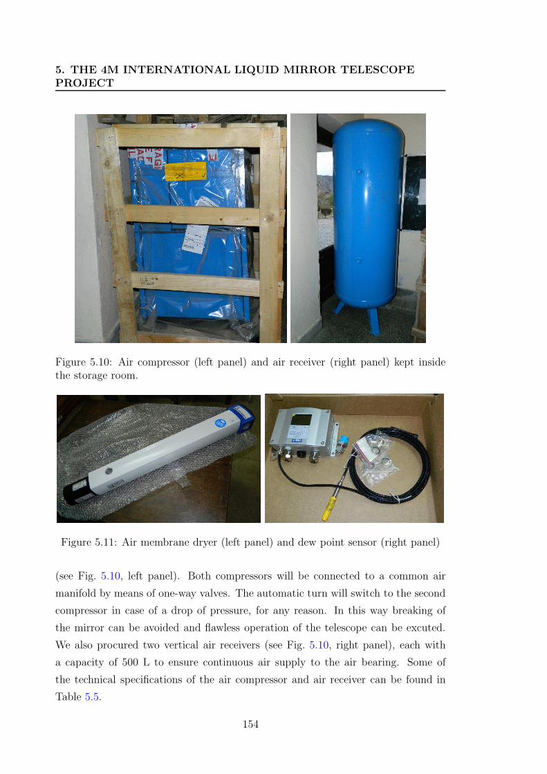
5. THE 4M INTERNATIONAL LIQUID MIRROR TELESCOPEPROJECT
Figure 5.10: Air compressor (left panel) and air receiver (right panel) kept insidethe storage room.
Figure 5.11: Air membrane dryer (left panel) and dew point sensor (right panel)
(see Fig. 5.10, left panel). Both compressors will be connected to a common air
manifold by means of one-way valves. The automatic turn will switch to the second
compressor in case of a drop of pressure, for any reason. In this way breaking of
the mirror can be avoided and flawless operation of the telescope can be excuted.
We also procured two vertical air receivers (see Fig. 5.10, right panel), each with
a capacity of 500 L to ensure continuous air supply to the air bearing. Some of
the technical specifications of the air compressor and air receiver can be found in
Table 5.5.
154
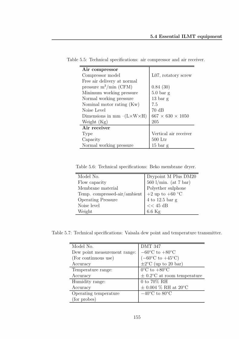
5.4 Essential ILMT equipment
Table 5.5: Technical specifications: air compressor and air receiver.
Air compressorCompressor model L07, rotatory screwFree air delivery at normalpressure m3/min (CFM) 0.84 (30)Minimum working pressure 5.0 bar gNormal working pressure 13 bar gNominal motor rating (Kw) 7.5Noise Level 70 dBDimensions in mm –(L×W×H) 667 × 630 × 1050Weight (Kg) 205Air receiverType Vertical air receiverCapacity 500 LtrNormal working pressure 15 bar g
Table 5.6: Technical specifications: Beko membrane dryer.
Model No. Drypoint M Plus DM20Flow capacity 560 l/min. (at 7 bar)Membrane material Polyether sulphoneTemp. compressed-air/ambient +2 up to +60 COperating Pressure 4 to 12.5 bar gNoise level << 45 dBWeight 6.6 Kg
Table 5.7: Technical specifications: Vaisala dew point and temperature transmitter.
Model No. DMT 347Dew point measurement range: −60C to +80C(For continuous use) (−60C to +45C)Accuracy ±2C (up to 20 bar)Temperature range: 0C to +80CAccuracy ± 0.2C at room temperatureHumidity range: 0 to 70% RHAccuracy ± 0.004 % RH at 20COperating temperature −40C to 80C(for probes)
155
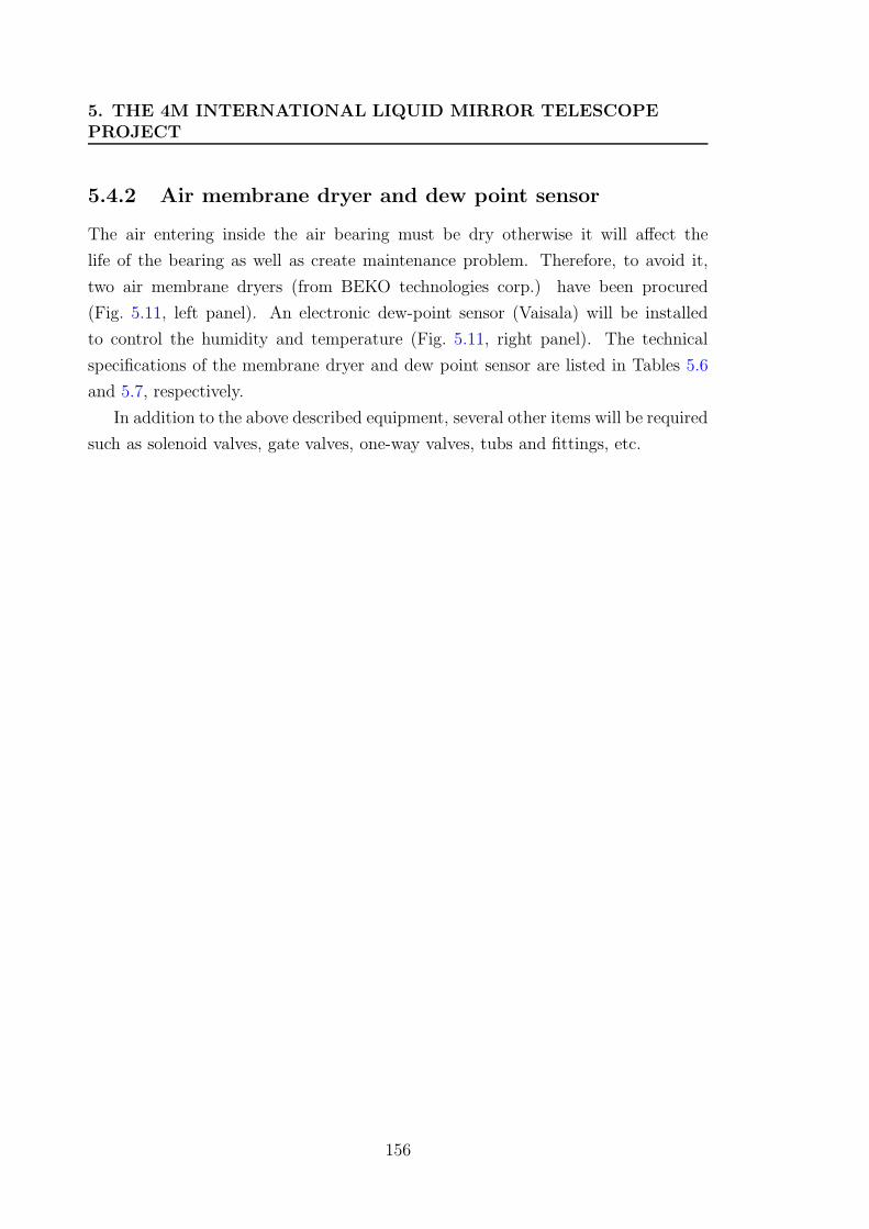
5. THE 4M INTERNATIONAL LIQUID MIRROR TELESCOPEPROJECT
5.4.2 Air membrane dryer and dew point sensor
The air entering inside the air bearing must be dry otherwise it will affect the
life of the bearing as well as create maintenance problem. Therefore, to avoid it,
two air membrane dryers (from BEKO technologies corp.) have been procured
(Fig. 5.11, left panel). An electronic dew-point sensor (Vaisala) will be installed
to control the humidity and temperature (Fig. 5.11, right panel). The technical
specifications of the membrane dryer and dew point sensor are listed in Tables 5.6
and 5.7, respectively.
In addition to the above described equipment, several other items will be required
such as solenoid valves, gate valves, one-way valves, tubs and fittings, etc.
156
Chapter 6
Preliminary tests with the 4m
ILMT
In this section we discuss various procedures which were carried out during the
developmental process of the ILMT. It includes reinforcement of the container, spin
casting of the primary mirror, mercury tests and mylar film tests.
6.1 Container reinforcement
The ILMT primary mirror is a composite structure constructed of bi-directional
carbon fiber cloth-epoxy skin over a closed-cell foam core. The principal elements
are a concave upper shell, of uniform thickness, supported by 12 radial ribs. The air
bearing interface presently employed by AMOS is a thin aluminum plate attached
to the bottom of the ribs by six M6 machine screws anchored with blind nuts glued
to the back of the lower skin. The plate is attached to the air bearing by three
bolts whose lengths can be adjusted. The mass of the composite structure alone
was measured by AMOS to be 210 kg (before spincasting). Although the composite
structure was quite strong and stiff, it was found after the tests that the interface
was not strong enough so that it could support an axial load of about 1000 kg
(including the weight of epoxy and mercury).
157
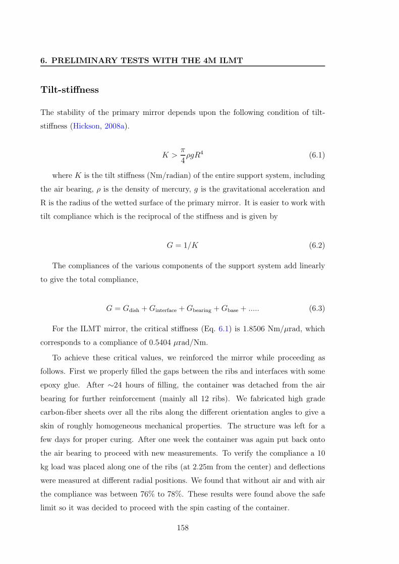
6. PRELIMINARY TESTS WITH THE 4M ILMT
Tilt-stiffness
The stability of the primary mirror depends upon the following condition of tilt-
stiffness (Hickson, 2008a).
K >π
4ρgR4 (6.1)
where K is the tilt stiffness (Nm/radian) of the entire support system, including
the air bearing, ρ is the density of mercury, g is the gravitational acceleration and
R is the radius of the wetted surface of the primary mirror. It is easier to work with
tilt compliance which is the reciprocal of the stiffness and is given by
G = 1/K (6.2)
The compliances of the various components of the support system add linearly
to give the total compliance,
G = Gdish +Ginterface +Gbearing +Gbase + ..... (6.3)
For the ILMT mirror, the critical stiffness (Eq. 6.1) is 1.8506 Nm/µrad, which
corresponds to a compliance of 0.5404 µrad/Nm.
To achieve these critical values, we reinforced the mirror while proceeding as
follows. First we properly filled the gaps between the ribs and interfaces with some
epoxy glue. After ∼24 hours of filling, the container was detached from the air
bearing for further reinforcement (mainly all 12 ribs). We fabricated high grade
carbon-fiber sheets over all the ribs along the different orientation angles to give a
skin of roughly homogeneous mechanical properties. The structure was left for a
few days for proper curing. After one week the container was again put back onto
the air bearing to proceed with new measurements. To verify the compliance a 10
kg load was placed along one of the ribs (at 2.25m from the center) and deflections
were measured at different radial positions. We found that without air and with air
the compliance was between 76% to 78%. These results were found above the safe
limit so it was decided to proceed with the spin casting of the container.
158
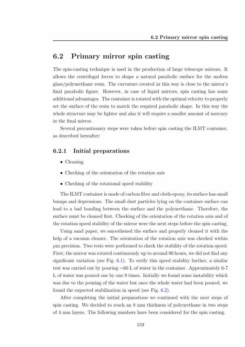
6.2 Primary mirror spin casting
6.2 Primary mirror spin casting
The spin-casting technique is used in the production of large telescope mirrors. It
allows the centrifugal forces to shape a natural parabolic surface for the molten
glass/polyurethane resin. The curvature created in this way is close to the mirror’s
final parabolic figure. However, in case of liquid mirrors, spin casting has some
additional advantages. The container is rotated with the optimal velocity to properly
set the surface of the resin to match the required parabolic shape. In this way the
whole structure may be lighter and also it will require a smaller amount of mercury
in the final mirror.
Several precautionary steps were taken before spin casting the ILMT container,
as described hereafter:
6.2.1 Initial preparations
• Cleaning
• Checking of the orientation of the rotation axis
• Checking of the rotational speed stability
The ILMT container is made of carbon fiber and cloth-epoxy, its surface has small
bumps and depressions. The small dust particles lying on the container surface can
lead to a bad bonding between the surface and the polyurethane. Therefore, the
surface must be cleaned first. Checking of the orientation of the rotation axis and of
the rotation speed stability of the mirror were the next steps before the spin casting.
Using sand paper, we smoothened the surface and properly cleaned it with the
help of a vacuum cleaner. The orientation of the rotation axis was checked within
µm precision. Two tests were performed to check the stability of the rotation speed.
First, the mirror was rotated continuously up to around 90 hours, we did not find any
significant variation (see Fig. 6.1). To verify this speed stability further, a similar
test was carried out by pouring ∼60 L of water in the container. Approximately 6-7
L of water was poured one by one 9 times. Initially we found some instability which
was due to the pouring of the water but once the whole water had been poured, we
found the expected stabilization in speed (see Fig. 6.2).
After completing the initial preparations we continued with the next steps of
spin casting. We decided to reach an 8 mm thickness of polyurethane in two steps
of 4 mm layers. The following numbers have been considered for the spin casting.
159
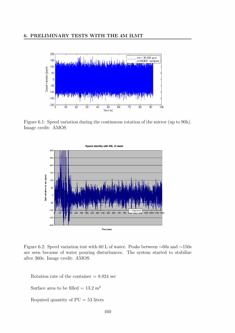
6. PRELIMINARY TESTS WITH THE 4M ILMT
Figure 6.1: Speed variation during the continuous rotation of the mirror (up to 90h).Image credit: AMOS
Figure 6.2: Speed variation test with 60 L of water. Peaks between ∼60s and ∼150sare seen because of water pouring disturbances. The system started to stabilizeafter 360s. Image credit: AMOS.
Rotation rate of the container = 8.024 sec
Surface area to be filled = 13.2 m2
Required quantity of PU = 53 liters
160
6.2 Primary mirror spin casting
Figure 6.3: Evolution of the PU temperature with time.
6.2.2 Final preparations
After these initial preparations, the container was ready for the final spin casting.
Polymerization test of PU
For a greater tear strength and more durability we used LS-30 A/B (a polyurethane
elastomer, product of BJB Enterprises, Inc.). It is resistant to moisture absorption
and cures easily at room temperature. Some of the other physical and chemical
properties are listed in Table 6.2. This product is available in two parts A and B.
To check the starting time of polymerization we made separately a small test. We
mixed up 8.8 liters of PU (45:100, A:B) and poured it in a tray. The temperature
variation with time was recorded (see Fig. 6.3). It is obvious from this figure that for
better bonding, we must complete the whole process of mixing and pouring within
15 minutes.
To mix and pour the PU within time, we decided to involve 6 persons. For a
proper pouring of PU over a 13.2 m2 surface area, the container was divided into 6
sections, each having an equal area of 2.199 m2 (see Fig. 6.4). The radial position
of each zone is given in Table 6.1. Each person was allowed to pour one section
only. When the polyurethane was poured on the mirror, the viscosity prevented a
fast spreading of the resin from one section to the next and finally we got a nearly
uniform surface with the required thickness. Before starting the spin casting, the
161
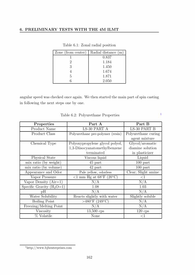
6. PRELIMINARY TESTS WITH THE 4M ILMT
Table 6.1: Zonal radial position
Zone (from center) Radial distance (m)1 0.8372 1.1843 1.4504 1.6745 1.8716 2.050
angular speed was checked once again. We then started the main part of spin casting
in following the next steps one by one.
Table 6.2: Polyurethane Properties 1
Properties Part A Part BProduct Name LS-30 PART A LS-30 PART BProduct Class Polyurethane pre-polymer (resin) Polyurethane curing
agent mixtureChemical Type Polyoxypropylene glycol polyol, Glycol/aromatic
1,3-Diisocyanatomethylbenzene diamine solutionterminated in plasticizer
Physical State Viscous liquid Liquidmix ratio (by weight) 45 part 100 partmix ratio (by volume) 42 part 100 partAppearance and Odor Pale yellow, odorless Clear; Slight amine
Vapor Pressure <1 mm Hg at 68F (20C) <1Vapor Density (Air=1) N/A N/A
Specific Gravity (H2O=1) 1.08 1.03pH N/A N/A
Water Solubility Reacts slightly with water Slightly solubleBoiling Point >480F (249C) N/A
Freezing/Melting Point N/A N/AViscosity 13,500 cps 120 cps% Volatile None <1
1http://www.bjbenterprises.com
162
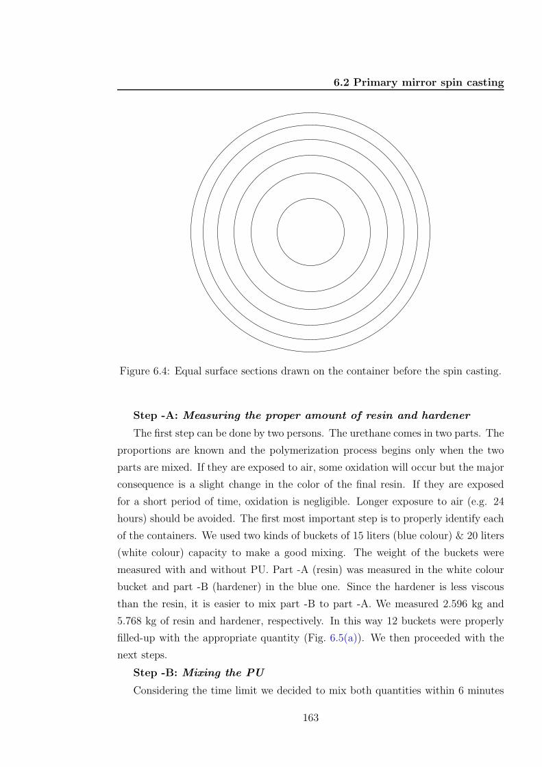
6.2 Primary mirror spin casting
Figure 6.4: Equal surface sections drawn on the container before the spin casting.
Step -A: Measuring the proper amount of resin and hardener
The first step can be done by two persons. The urethane comes in two parts. The
proportions are known and the polymerization process begins only when the two
parts are mixed. If they are exposed to air, some oxidation will occur but the major
consequence is a slight change in the color of the final resin. If they are exposed
for a short period of time, oxidation is negligible. Longer exposure to air (e.g. 24
hours) should be avoided. The first most important step is to properly identify each
of the containers. We used two kinds of buckets of 15 liters (blue colour) & 20 liters
(white colour) capacity to make a good mixing. The weight of the buckets were
measured with and without PU. Part -A (resin) was measured in the white colour
bucket and part -B (hardener) in the blue one. Since the hardener is less viscous
than the resin, it is easier to mix part -B to part -A. We measured 2.596 kg and
5.768 kg of resin and hardener, respectively. In this way 12 buckets were properly
filled-up with the appropriate quantity (Fig. 6.5(a)). We then proceeded with the
next steps.
Step -B: Mixing the PU
Considering the time limit we decided to mix both quantities within 6 minutes
163
6. PRELIMINARY TESTS WITH THE 4M ILMT
(a)
(b)
Figure 6.5: Spin casting preparation. (a) Measured quantity of PU: Base resin, part-A (white bucket) and hardener part -B (blue bucket). (b) PU mixing process.
(Fig. 6.5(b)). A signal was given to mix part B in part A. This was done within 2
minutes and during the remaining 4 minutes, the whole liquid was homogeneously
mixed by a hand held wooden mixer. It is very important to give at least ∼10%
of time to scrape the side and the bottom of the bucket at the same time to avoid
formation of bubbles in the process.
Step -C: Pouring the PU over the container surface
Once the PU is mixed properly, the next step consisted in pouring it over the
surface of the container. To pour each sector (as described previously), 4 persons
used a ladder which was lying above the container and 2 persons near two opposite
sides of the mirror (see Fig. 6.6). Due to its high viscosity all the resin will spread
over each annular sector. Some small holes may remain on the container surface
but they will eventually filled-up. The resin takes about ∼24 hours to polymerize
164

6.3 Mercury tests: constructing the liquid mirror
Figure 6.6: Pouring of the PU over the surface of the container. Each of the sixsectors were poured at the same time with the continuously rotating container.
adequately however, complete polymerization will take much longer time. We left
the rotating mirror for 24 hours for a perfect bonding.
6.3 Mercury tests: constructing the liquid mirror
In this section we present a short description about various liquids which have the
ability to be used for LM and various safety equipments that were used in the process
of mercury tests.
6.3.1 Mercury as a reflecting liquid
Mostly metals are good reflectors. To fabricate a rotating mirror a metal can be
used which is liquid at the room temperature and at the same time it must be highly
reflective. Francium (Fr), Cesium (Cs), Gallium (Ga) and Rubidium (Rb) melt a few
degrees above room temperature but Bromine (Br), and Mercury (Hg) are liquid at
room temperature. Laboratory experiments have shown that mercury, gallium, and
165
6. PRELIMINARY TESTS WITH THE 4M ILMT
gallium-indium can be used to construct LMTs but these liquids have advantages
and disadvantages relative to each other. Extensive tests of gallium, and gallium-
indium LMs have been examined by Borra et al. (1997). They found that the image
quality of Ga LM is comparable to that of Hg LM. But the use of Ga requires a
particular process, like supercooling. Also Gallium oxidizes very rapidly and forms
a transparent thin oxide skin that protects the liquid from additional oxidation.
However, this skin is repeatedly broken upon start-up, ruining the optical quality
of the mirror. This has been a major problem with Ga LM.
Mercury is a naturally occurring metal and exists in various forms: elemental (or
metallic); inorganic (e.g. mercuric sulphide, mercuric oxide and mercuric chloride);
and organic (e.g. methyl- and ethylmercury). Some of the properties of mercury are
mentioned in Table 6.3.2. Mercury has a reflectivity between ∼75 to ∼78 percent in
the wavelength range of 4000A– 10000A (see Boiani & Rice, 1969). This corresponds
to 90 percent of the reflectivity of an aluminium-coated glass mirror. Therefore, in
general mercury has been used primarily for constructing LMTs. It must be noted
that human exposure to all forms of mercury is toxic however, the toxicity and
implications depend upon its chemical form and the route of exposure. Both the
liquid and vapors of elemental mercury are poorly absorbed through the skin but
the vapors can be highly toxic if inhaled.
The toxic mercury vapors are greatly reduced after 7-8 hours, thanks to a mer-
cury oxide layer which forms when the mercury reacts with the ambient air. Once
it is created, the oxide layer “reinforces” the mirror as it prevents the surface to
break because of small perturbations such as insects/dust falling on the mercury.
Figure 6.7 represents the mercury vapor concentration as a function of time for the
NASA liquid mirror at NODO. The initial peak (∼200 min) is because the mirror
was halted after rotation otherwise mercury oxide layer could have begun to form to
suppress these vapors. At ∼1350 min the mirror was cleaned and reformed. Then
after around 8 hours a thin mercury oxide layer keeps the vapor below the Oc-
cupational Safety and Health Administration, U.S. (OSHA) limit (25µg/m3, pink
horizontal line).
6.3.2 Mercury exposure limit
Various organizations have set different threshold limit values1 (TLV). The Scien-
tific Committee on Occupational Exposure Limits for elemental mercury and inor-
1Daily exposure level above which it is believed a worker could suffer adverse health effects
166
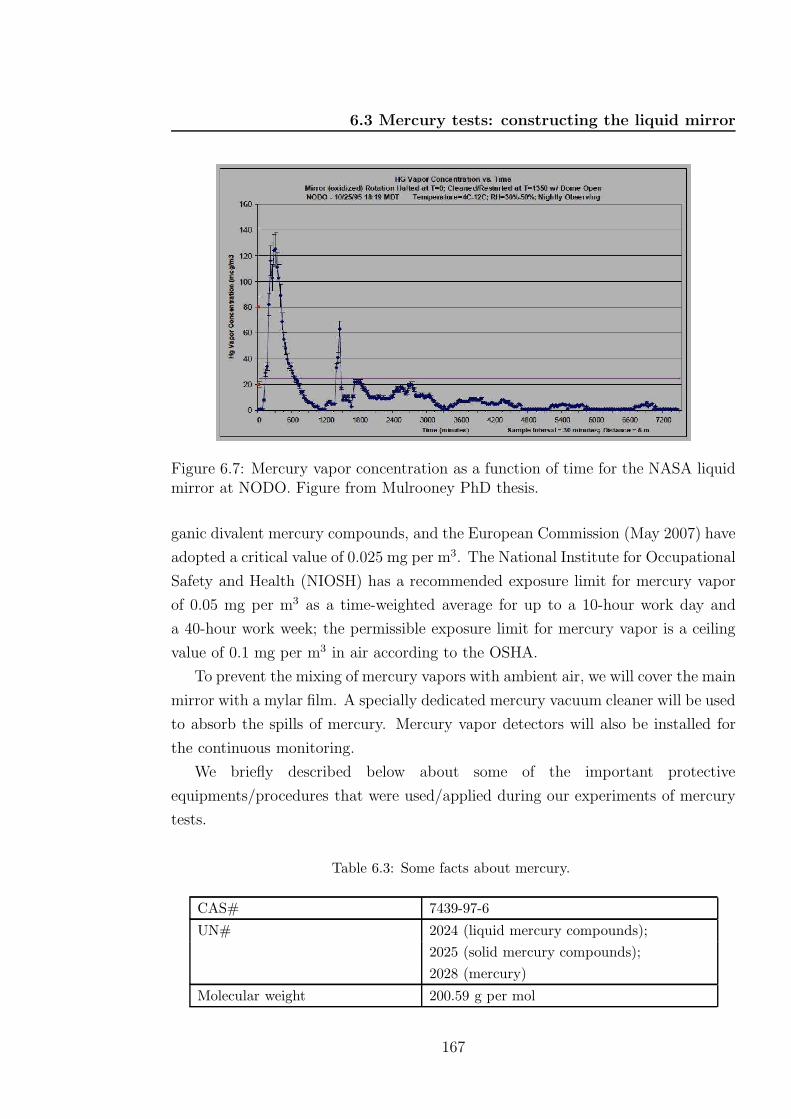
6.3 Mercury tests: constructing the liquid mirror
Figure 6.7: Mercury vapor concentration as a function of time for the NASA liquidmirror at NODO. Figure from Mulrooney PhD thesis.
ganic divalent mercury compounds, and the European Commission (May 2007) have
adopted a critical value of 0.025 mg per m3. The National Institute for Occupational
Safety and Health (NIOSH) has a recommended exposure limit for mercury vapor
of 0.05 mg per m3 as a time-weighted average for up to a 10-hour work day and
a 40-hour work week; the permissible exposure limit for mercury vapor is a ceiling
value of 0.1 mg per m3 in air according to the OSHA.
To prevent the mixing of mercury vapors with ambient air, we will cover the main
mirror with a mylar film. A specially dedicated mercury vacuum cleaner will be used
to absorb the spills of mercury. Mercury vapor detectors will also be installed for
the continuous monitoring.
We briefly described below about some of the important protective
equipments/procedures that were used/applied during our experiments of mercury
tests.
Table 6.3: Some facts about mercury.
CAS# 7439-97-6
UN# 2024 (liquid mercury compounds);
2025 (solid mercury compounds);
2028 (mercury)
Molecular weight 200.59 g per mol
167
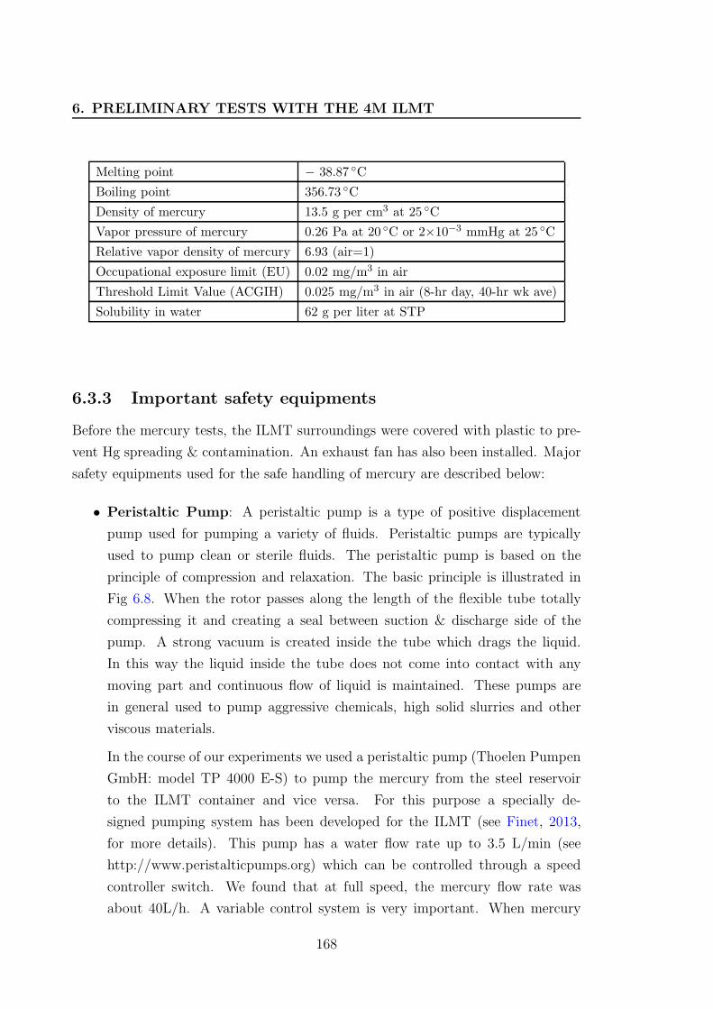
6. PRELIMINARY TESTS WITH THE 4M ILMT
Melting point − 38.87 C
Boiling point 356.73 C
Density of mercury 13.5 g per cm3 at 25 C
Vapor pressure of mercury 0.26 Pa at 20 C or 2×10⁻³ mmHg at 25 C
Relative vapor density of mercury 6.93 (air=1)
Occupational exposure limit (EU) 0.02 mg/m3 in air
Threshold Limit Value (ACGIH) 0.025 mg/m3 in air (8-hr day, 40-hr wk ave)
Solubility in water 62 g per liter at STP
6.3.3 Important safety equipments
Before the mercury tests, the ILMT surroundings were covered with plastic to pre-
vent Hg spreading & contamination. An exhaust fan has also been installed. Major
safety equipments used for the safe handling of mercury are described below:
• Peristaltic Pump: A peristaltic pump is a type of positive displacement
pump used for pumping a variety of fluids. Peristaltic pumps are typically
used to pump clean or sterile fluids. The peristaltic pump is based on the
principle of compression and relaxation. The basic principle is illustrated in
Fig 6.8. When the rotor passes along the length of the flexible tube totally
compressing it and creating a seal between suction & discharge side of the
pump. A strong vacuum is created inside the tube which drags the liquid.
In this way the liquid inside the tube does not come into contact with any
moving part and continuous flow of liquid is maintained. These pumps are
in general used to pump aggressive chemicals, high solid slurries and other
viscous materials.
In the course of our experiments we used a peristaltic pump (Thoelen Pumpen
GmbH: model TP 4000 E-S) to pump the mercury from the steel reservoir
to the ILMT container and vice versa. For this purpose a specially de-
signed pumping system has been developed for the ILMT (see Finet, 2013,
for more details). This pump has a water flow rate up to 3.5 L/min (see
http://www.peristalticpumps.org) which can be controlled through a speed
controller switch. We found that at full speed, the mercury flow rate was
about 40L/h. A variable control system is very important. When mercury
168
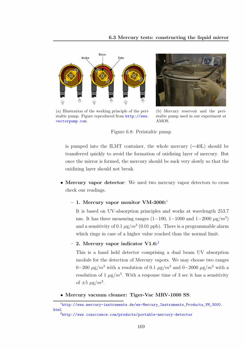
6.3 Mercury tests: constructing the liquid mirror
(a) Illustration of the working principle of the peri-staltic pump. Figure reproduced from http://www.
vectorpump.com.
(b) Mercury reservoir and the peri-staltic pump used in our experiment atAMOS.
Figure 6.8: Peristaltic pump
is pumped into the ILMT container, the whole mercury (∼40L) should be
transferred quickly to avoid the formation of oxidizing layer of mercury. But
once the mirror is formed, the mercury should be suck very slowly so that the
oxidizing layer should not break.
• Mercury vapor detector: We used two mercury vapor detectors to cross
check our readings.
– 1. Mercury vapor monitor VM-3000:1
It is based on UV-absorption principles and works at wavelength 253.7
nm. It has three measuring ranges (1−100, 1−1000 and 1−2000 µg/m3)
and a sensitivity of 0.1 µg/m3 (0.01 ppb). There is a programmable alarm
which rings in case of a higher value reached than the normal limit.
– 2. Mercury vapor indicator V1.6:2
This is a hand held detector comprising a dual beam UV absorption
module for the detection of Mercury vapors. We may choose two ranges
0−200 µg/m3 with a resolution of 0.1 µg/m3 and 0−2000 µg/m3 with a
resolution of 1 µg/m3. With a response time of 3 sec it has a sensitivity
of ±5 µg/m3.
• Mercury vacuum cleaner: Tiger-Vac MRV-1000 SS:
1http://www.mercury-instruments.de/en-Mercury_Instruments_Products_VM_3000.
html2http://www.ionscience.com/products/portable-mercury-detector
169
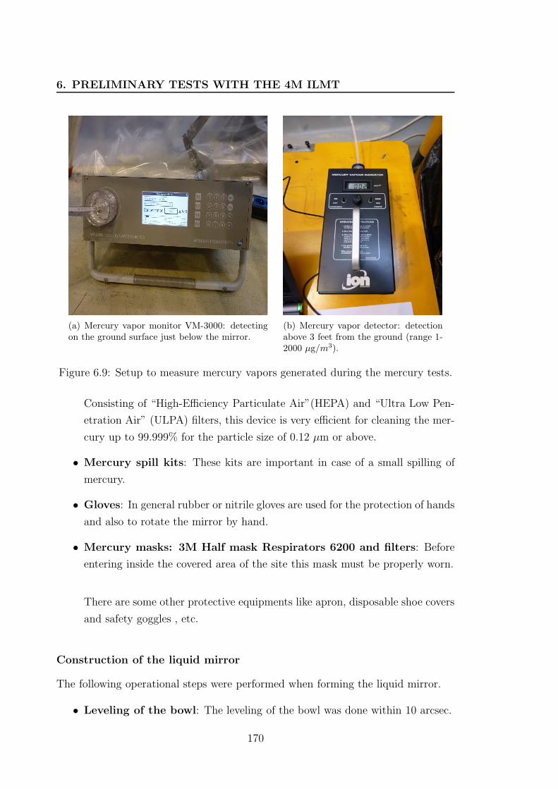
6. PRELIMINARY TESTS WITH THE 4M ILMT
(a) Mercury vapor monitor VM-3000: detectingon the ground surface just below the mirror.
(b) Mercury vapor detector: detectionabove 3 feet from the ground (range 1-2000 µg/m3).
Figure 6.9: Setup to measure mercury vapors generated during the mercury tests.
Consisting of “High-Efficiency Particulate Air”(HEPA) and “Ultra Low Pen-
etration Air” (ULPA) filters, this device is very efficient for cleaning the mer-
cury up to 99.999% for the particle size of 0.12 µm or above.
• Mercury spill kits: These kits are important in case of a small spilling of
mercury.
• Gloves: In general rubber or nitrile gloves are used for the protection of hands
and also to rotate the mirror by hand.
• Mercury masks: 3M Half mask Respirators 6200 and filters: Before
entering inside the covered area of the site this mask must be properly worn.
There are some other protective equipments like apron, disposable shoe covers
and safety goggles , etc.
Construction of the liquid mirror
The following operational steps were performed when forming the liquid mirror.
• Leveling of the bowl: The leveling of the bowl was done within 10 arcsec.
170
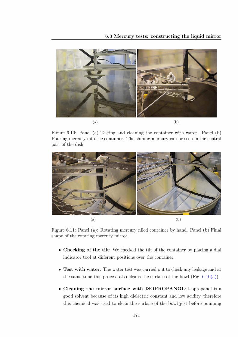
6.3 Mercury tests: constructing the liquid mirror
(a) (b)
Figure 6.10: Panel (a) Testing and cleaning the container with water. Panel (b)Pouring mercury into the container. The shining mercury can be seen in the centralpart of the dish.
(a) (b)
Figure 6.11: Panel (a): Rotating mercury filled container by hand. Panel (b) Finalshape of the rotating mercury mirror.
• Checking of the tilt: We checked the tilt of the container by placing a dial
indicator tool at different positions over the container.
• Test with water: The water test was carried out to check any leakage and at
the same time this process also cleans the surface of the bowl (Fig. 6.10(a)).
• Cleaning the mirror surface with ISOPROPANOL: Isopropanol is a
good solvent because of its high dielectric constant and low acidity, therefore
this chemical was used to clean the surface of the bowl just before pumping
171
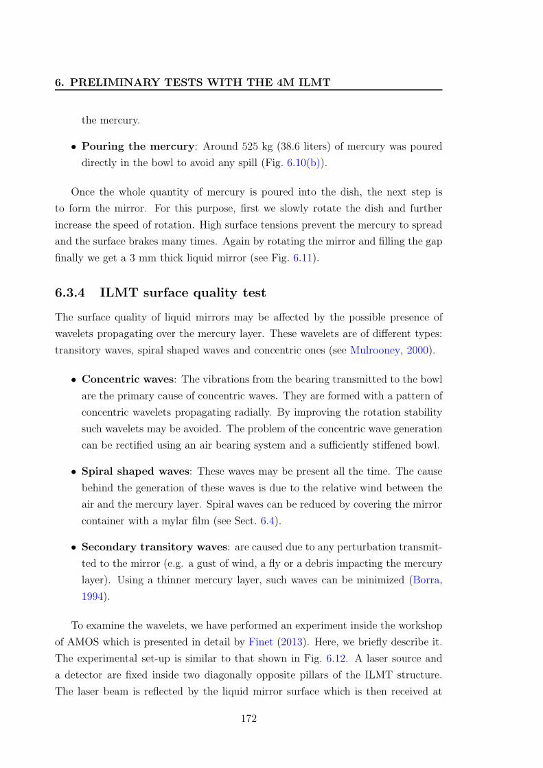
6. PRELIMINARY TESTS WITH THE 4M ILMT
the mercury.
• Pouring the mercury: Around 525 kg (38.6 liters) of mercury was poured
directly in the bowl to avoid any spill (Fig. 6.10(b)).
Once the whole quantity of mercury is poured into the dish, the next step is
to form the mirror. For this purpose, first we slowly rotate the dish and further
increase the speed of rotation. High surface tensions prevent the mercury to spread
and the surface brakes many times. Again by rotating the mirror and filling the gap
finally we get a 3 mm thick liquid mirror (see Fig. 6.11).
6.3.4 ILMT surface quality test
The surface quality of liquid mirrors may be affected by the possible presence of
wavelets propagating over the mercury layer. These wavelets are of different types:
transitory waves, spiral shaped waves and concentric ones (see Mulrooney, 2000).
• Concentric waves: The vibrations from the bearing transmitted to the bowl
are the primary cause of concentric waves. They are formed with a pattern of
concentric wavelets propagating radially. By improving the rotation stability
such wavelets may be avoided. The problem of the concentric wave generation
can be rectified using an air bearing system and a sufficiently stiffened bowl.
• Spiral shaped waves: These waves may be present all the time. The cause
behind the generation of these waves is due to the relative wind between the
air and the mercury layer. Spiral waves can be reduced by covering the mirror
container with a mylar film (see Sect. 6.4).
• Secondary transitory waves: are caused due to any perturbation transmit-
ted to the mirror (e.g. a gust of wind, a fly or a debris impacting the mercury
layer). Using a thinner mercury layer, such waves can be minimized (Borra,
1994).
To examine the wavelets, we have performed an experiment inside the workshop
of AMOS which is presented in detail by Finet (2013). Here, we briefly describe it.
The experimental set-up is similar to that shown in Fig. 6.12. A laser source and
a detector are fixed inside two diagonally opposite pillars of the ILMT structure.
The laser beam is reflected by the liquid mirror surface which is then received at
172
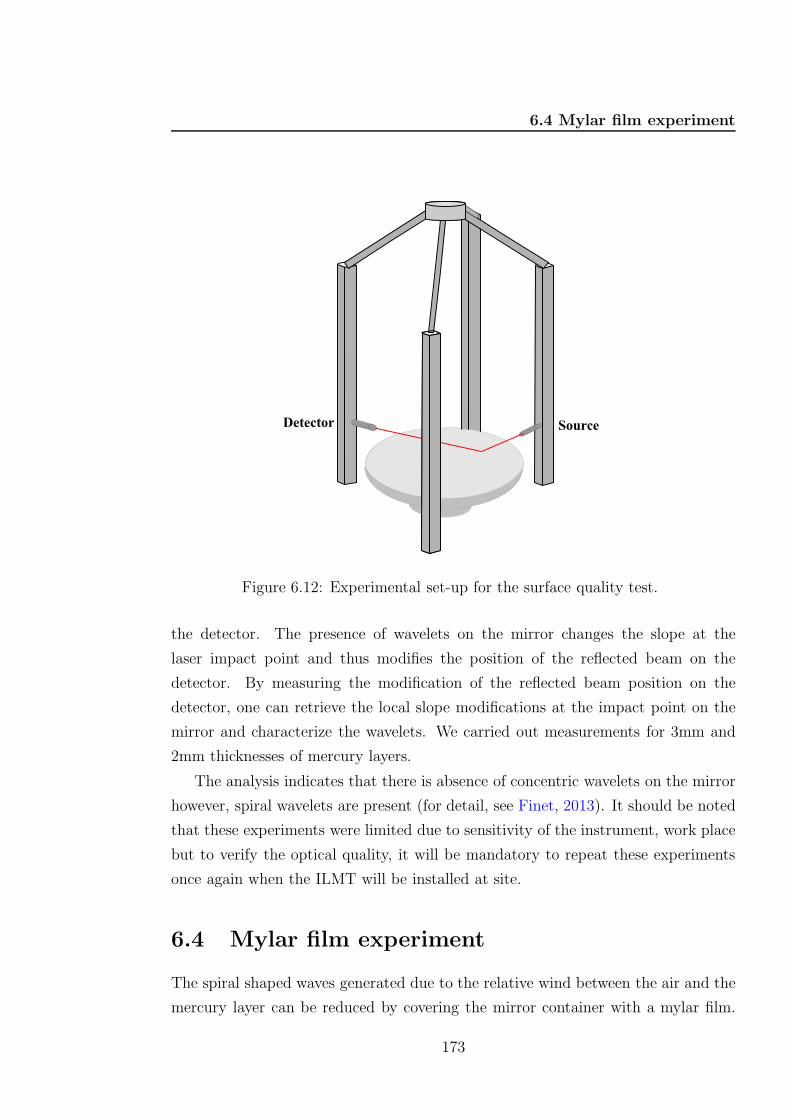
6.4 Mylar film experiment
Figure 6.12: Experimental set-up for the surface quality test.
the detector. The presence of wavelets on the mirror changes the slope at the
laser impact point and thus modifies the position of the reflected beam on the
detector. By measuring the modification of the reflected beam position on the
detector, one can retrieve the local slope modifications at the impact point on the
mirror and characterize the wavelets. We carried out measurements for 3mm and
2mm thicknesses of mercury layers.
The analysis indicates that there is absence of concentric wavelets on the mirror
however, spiral wavelets are present (for detail, see Finet, 2013). It should be noted
that these experiments were limited due to sensitivity of the instrument, work place
but to verify the optical quality, it will be mandatory to repeat these experiments
once again when the ILMT will be installed at site.
6.4 Mylar film experiment
The spiral shaped waves generated due to the relative wind between the air and the
mercury layer can be reduced by covering the mirror container with a mylar film.
173
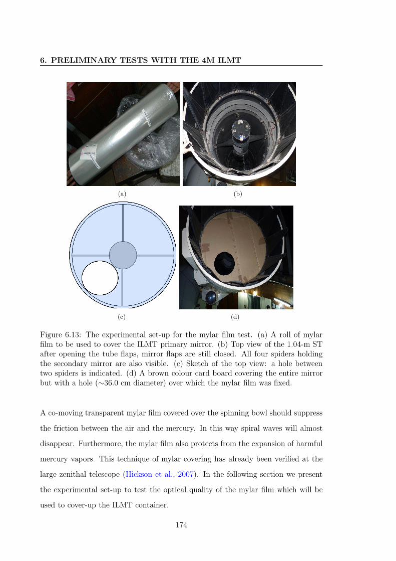
6. PRELIMINARY TESTS WITH THE 4M ILMT
(a) (b)
(c) (d)
Figure 6.13: The experimental set-up for the mylar film test. (a) A roll of mylarfilm to be used to cover the ILMT primary mirror. (b) Top view of the 1.04-m STafter opening the tube flaps, mirror flaps are still closed. All four spiders holdingthe secondary mirror are also visible. (c) Sketch of the top view: a hole betweentwo spiders is indicated. (d) A brown colour card board covering the entire mirrorbut with a hole (∼36.0 cm diameter) over which the mylar film was fixed.
A co-moving transparent mylar film covered over the spinning bowl should suppress
the friction between the air and the mercury. In this way spiral waves will almost
disappear. Furthermore, the mylar film also protects from the expansion of harmful
mercury vapors. This technique of mylar covering has already been verified at the
large zenithal telescope (Hickson et al., 2007). In the following section we present
the experimental set-up to test the optical quality of the mylar film which will be
used to cover-up the ILMT container.
174
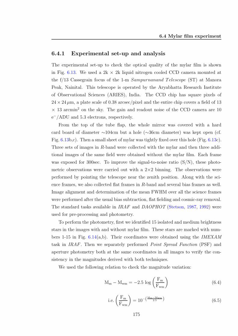
6.4 Mylar film experiment
6.4.1 Experimental set-up and analysis
The experimental set-up to check the optical quality of the mylar film is shown
in Fig. 6.13. We used a 2k × 2k liquid nitrogen cooled CCD camera mounted at
the f/13 Cassegrain focus of the 1-m Sampurnanand Telescope (ST) at Manora
Peak, Nainital. This telescope is operated by the Aryabhatta Research Institute
of Observational Sciences (ARIES), India. The CCD chip has square pixels of
24× 24µm, a plate scale of 0.38 arcsec/pixel and the entire chip covers a field of 13
× 13 arcmin2 on the sky. The gain and readout noise of the CCD camera are 10
e−/ADU and 5.3 electrons, respectively.
From the top of the tube flap, the whole mirror was covered with a hard
card board of diameter ∼104cm but a hole (∼36cm diameter) was kept open (cf.
Fig. 6.13b,c). Then a small sheet of mylar was tightly fixed over this hole (Fig. 6.13c).
Three sets of images in R-band were collected with the mylar and then three addi-
tional images of the same field were obtained without the mylar film. Each frame
was exposed for 300sec. To improve the signal-to-noise ratio (S/N), these photo-
metric observations were carried out with a 2×2 binning. The observations were
performed by pointing the telescope near the zenith position. Along with the sci-
ence frames, we also collected flat frames in R-band and several bias frames as well.
Image alignment and determination of the mean FWHM over all the science frames
were performed after the usual bias subtraction, flat fielding and cosmic-ray removal.
The standard tasks available in IRAF and DAOPHOT (Stetson, 1987, 1992) were
used for pre-processing and photometry.
To perform the photometry, first we identified 15 isolated and medium brightness
stars in the images with and without mylar film. These stars are marked with num-
bers 1-15 in Fig. 6.14(a,b). Their coordinates were obtained using the IMEXAM
task in IRAF . Then we separately performed Point Spread Function (PSF) and
aperture photometry both at the same coordinates in all images to verify the con-
sistency in the magnitudes derived with both techniques.
We used the following relation to check the magnitude variation:
Mm −Mwm = −2.5 log
(
Fm
Fwm
)
(6.4)
i.e.
(
Fm
Fwm
)
= 10−(Mm−Mwm
2.5 ) (6.5)
175
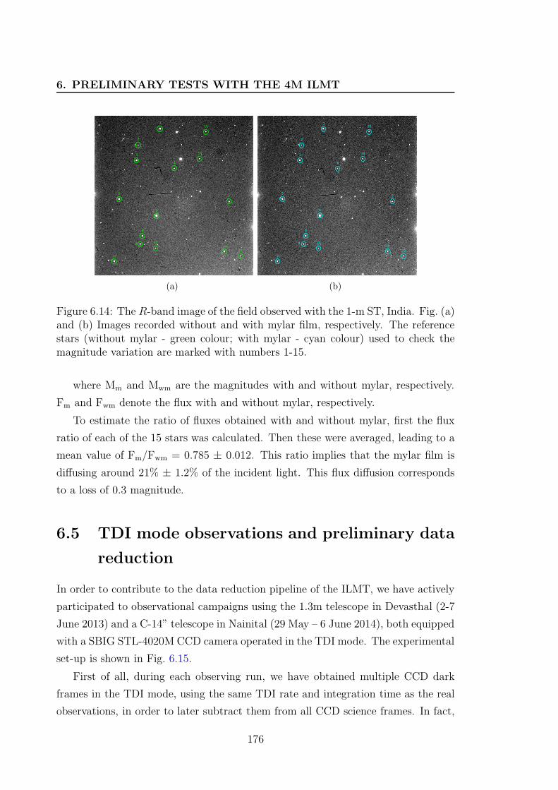
6. PRELIMINARY TESTS WITH THE 4M ILMT
9
15
14
1312
11
10
8
7
6
5
4
3
2
1
(a)
9
15
14
1312
11
10
8
7
6
5
4
3
2
1
(b)
Figure 6.14: The R-band image of the field observed with the 1-m ST, India. Fig. (a)and (b) Images recorded without and with mylar film, respectively. The referencestars (without mylar - green colour; with mylar - cyan colour) used to check themagnitude variation are marked with numbers 1-15.
where Mm and Mwm are the magnitudes with and without mylar, respectively.
Fm and Fwm denote the flux with and without mylar, respectively.
To estimate the ratio of fluxes obtained with and without mylar, first the flux
ratio of each of the 15 stars was calculated. Then these were averaged, leading to a
mean value of Fm/Fwm = 0.785 ± 0.012. This ratio implies that the mylar film is
diffusing around 21% ± 1.2% of the incident light. This flux diffusion corresponds
to a loss of 0.3 magnitude.
6.5 TDI mode observations and preliminary data
reduction
In order to contribute to the data reduction pipeline of the ILMT, we have actively
participated to observational campaigns using the 1.3m telescope in Devasthal (2-7
June 2013) and a C-14” telescope in Nainital (29 May – 6 June 2014), both equipped
with a SBIG STL-4020M CCD camera operated in the TDI mode. The experimental
set-up is shown in Fig. 6.15.
First of all, during each observing run, we have obtained multiple CCD dark
frames in the TDI mode, using the same TDI rate and integration time as the real
observations, in order to later subtract them from all CCD science frames. In fact,
176
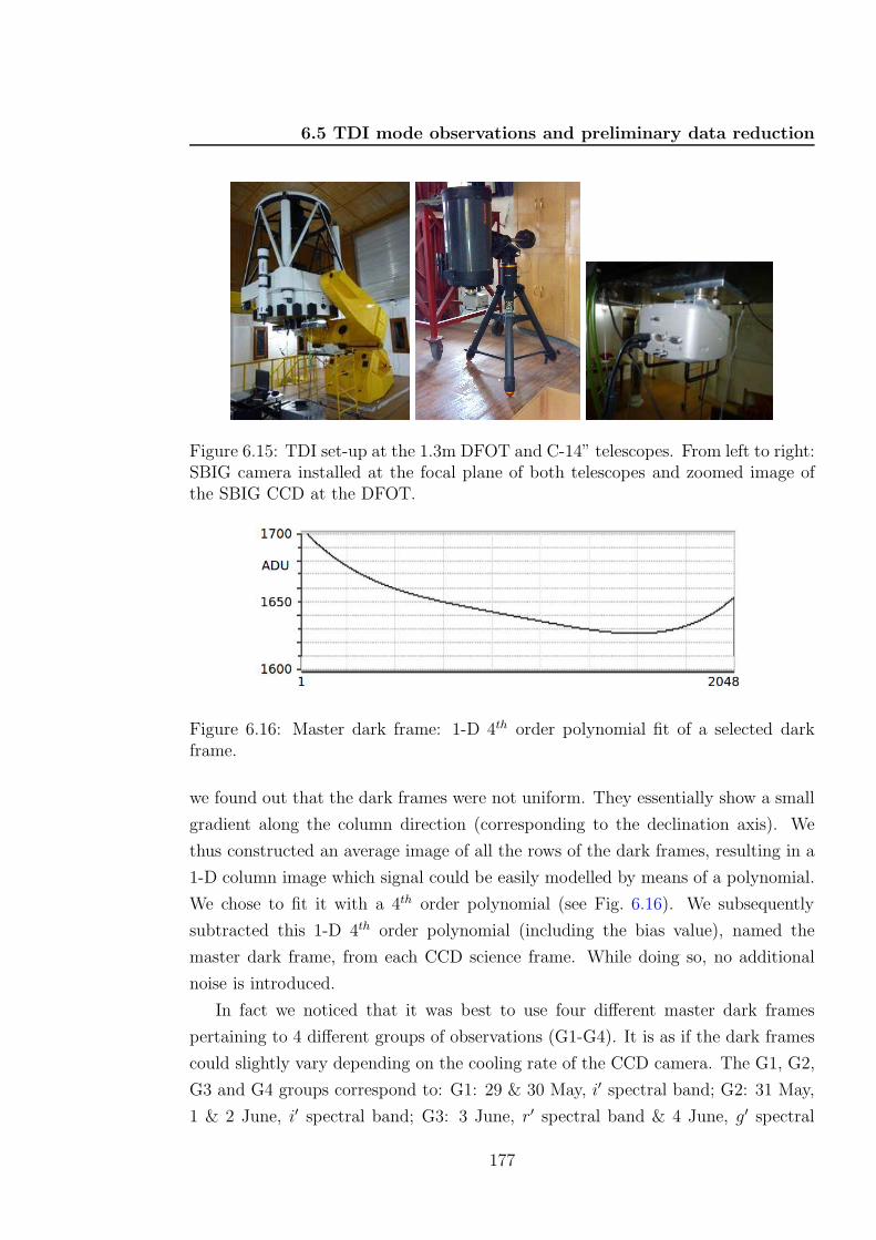
6.5 TDI mode observations and preliminary data reduction
Figure 6.15: TDI set-up at the 1.3m DFOT and C-14” telescopes. From left to right:SBIG camera installed at the focal plane of both telescopes and zoomed image ofthe SBIG CCD at the DFOT.
Figure 6.16: Master dark frame: 1-D 4th order polynomial fit of a selected darkframe.
we found out that the dark frames were not uniform. They essentially show a small
gradient along the column direction (corresponding to the declination axis). We
thus constructed an average image of all the rows of the dark frames, resulting in a
1-D column image which signal could be easily modelled by means of a polynomial.
We chose to fit it with a 4th order polynomial (see Fig. 6.16). We subsequently
subtracted this 1-D 4th order polynomial (including the bias value), named the
master dark frame, from each CCD science frame. While doing so, no additional
noise is introduced.
In fact we noticed that it was best to use four different master dark frames
pertaining to 4 different groups of observations (G1-G4). It is as if the dark frames
could slightly vary depending on the cooling rate of the CCD camera. The G1, G2,
G3 and G4 groups correspond to: G1: 29 & 30 May, i′ spectral band; G2: 31 May,
1 & 2 June, i′ spectral band; G3: 3 June, r′ spectral band & 4 June, g′ spectral
177
6. PRELIMINARY TESTS WITH THE 4M ILMT
band; G4: 6 June, i′ spectral band, 2014.
From each CCD science frame, we then constructed a flat field frame as fol-
lows. First of all, we subtracted from each column of the CCD science frames the
corresponding 1-D master dark frame.
Since the observations were taken in the TDI mode, all stellar images were
naturally trailed through all the columns of the CCD camera (30000 columns in our
case). This means that unlike for the case of classical CCD observations, but alike
for the master dark frame, the flat field frame needs to be just one-dimensional.
Typically, it was either obtained by taking the median value of each row of the
science CCD frames (excluding in this way all stellar objects and other defects like
cosmic rays, etc.). We similarly found out that it was even better to take the average
value of all individual rows of the science frames after applying a sigma clipping.
Considering the CCD frames obtained with the C-14” telescope in May-June 2014,
we found out that the best was to adopt a one-sigma clipping and 6 iterations. This
led to very nice results (see below).
The 1-D flat field frame is thus obtained using the background sky light of each
science frame which exposure time was typically 15 min. It could have been longer
but was limited (to 30000 columns) due to the RAM memory of the PC being used
to run the MaxImDL program when collecting the data in the TDI mode. This
ensures that when we shall deal with the photometry of very faint objects observed
in the TDI mode with the ILMT, the resulting flat field will be the most appropriate
one since the dominating light affecting the faint objects is mainly due to the sky
background. Constructing a 1-D flat field from so many columns (typically 30000
in our case during an average exposure time of approximately 15 minutes) ensures
a very good S/N ratio for the resulting flat fields.
We then normalized each individual 1-D flat field by their average value.
The G1, G2, G3 and G4 1-D master normalized flat fields were obtained by
taking the average of all 1-D normalized flat fields pertaining to each individual
science frame integrations belonging to those individual groups (see Fig. 6.17). All
resulting 1-D master normalized flat fields look very similar (even when considering
the different broadband filters i′, g′ and r′ that were used).
In summary, we recommend at this moment to flat field each science frame
using the normalized 1-D flat field obtained from their own sky background. After
checking that all those normalized 1-D flat fields are the same, one may of course
178

6.5 TDI mode observations and preliminary data reduction
Figure 6.17: Normalized 1-D flat fields for the 4 groups of observations. G1: 29 &30 May (i′); G2: 31 May, 1 & 2 June (i′); G3: 3 (r′) & 4 (g′) June: G4: 6 June (i′)2014.
Figure 6.18: Original (up) and flat fielded (down) CCD frame TDI-03-F3790-01-06-2014 recorded in the TDI mode (i′ spectral band) with the C-14” telescope on 1st
of June 2014. The horizontal and vertical graphs illustrate the flat response alongone arbitrarily chosen row and one column of the flat fielded frame.
construct a master flat field out of them and perform a final reduction of all science
observations.
An example of raw and flat fielded science frame obtained in the TDI mode with
the C-14” telescope equipped with a i′ filter is shown in Figs. 6.18 - 6.20. As it can
be seen, our proposed way of correcting CCD frames recorded in the TDI mode by
means of a 1-D normalized flat field looks very promising.
Photometric and astrometric measurements of objects detected on those reduced
frames were later performed using standard IRAF applications.
179
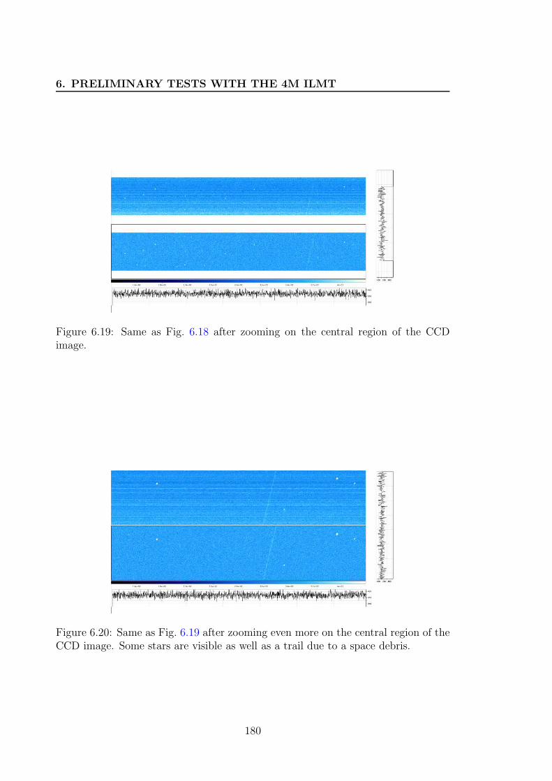
6. PRELIMINARY TESTS WITH THE 4M ILMT
Figure 6.19: Same as Fig. 6.18 after zooming on the central region of the CCDimage.
Figure 6.20: Same as Fig. 6.19 after zooming even more on the central region of theCCD image. Some stars are visible as well as a trail due to a space debris.
180
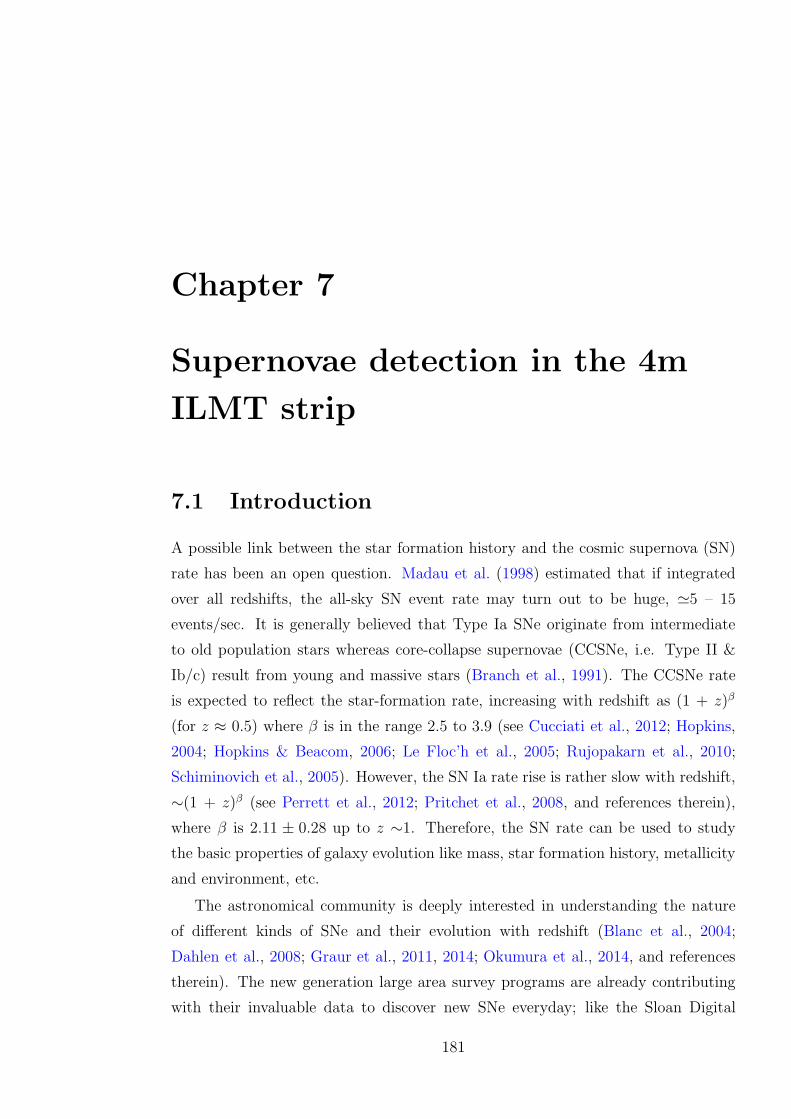
Chapter 7
Supernovae detection in the 4m
ILMT strip
7.1 Introduction
A possible link between the star formation history and the cosmic supernova (SN)
rate has been an open question. Madau et al. (1998) estimated that if integrated
over all redshifts, the all-sky SN event rate may turn out to be huge, ≃5 – 15
events/sec. It is generally believed that Type Ia SNe originate from intermediate
to old population stars whereas core-collapse supernovae (CCSNe, i.e. Type II &
Ib/c) result from young and massive stars (Branch et al., 1991). The CCSNe rate
is expected to reflect the star-formation rate, increasing with redshift as (1 + z)β
(for z ≈ 0.5) where β is in the range 2.5 to 3.9 (see Cucciati et al., 2012; Hopkins,
2004; Hopkins & Beacom, 2006; Le Floc’h et al., 2005; Rujopakarn et al., 2010;
Schiminovich et al., 2005). However, the SN Ia rate rise is rather slow with redshift,
∼(1 + z)β (see Perrett et al., 2012; Pritchet et al., 2008, and references therein),
where β is 2.11 ± 0.28 up to z ∼1. Therefore, the SN rate can be used to study
the basic properties of galaxy evolution like mass, star formation history, metallicity
and environment, etc.
The astronomical community is deeply interested in understanding the nature
of different kinds of SNe and their evolution with redshift (Blanc et al., 2004;
Dahlen et al., 2008; Graur et al., 2011, 2014; Okumura et al., 2014, and references
therein). The new generation large area survey programs are already contributing
with their invaluable data to discover new SNe everyday; like the Sloan Digital
181
7. SUPERNOVAE DETECTION IN THE 4M ILMT STRIP
Sky Survey1 (SDSS), Supernova Cosmology Project2 (SCP) and intermediate Palo-
mar Transient Factory3 (iPTF), Supernova Legacy Survey4 (SNLS), Catalina Real-
Time Transient Survey5 (CRTS), Southern inTermediate Redshift ESO Supernova
Search (STRESS), Panoramic Survey Telescope & Rapid Response System6 (Pan-
STARRS) etc. Some upcoming facilities will continue to grow these efforts such as
the Large Synoptic Survey Telescope7 (LSST) and the Zwicky Transient Facility8
(ZTF), SkyMapper9 All-Sky Automated Survey for Supernovae10 (ASAS-SN).
It is notable that despite their great contribution to SN search programs, these
kinds of projects are observationally expensive, requiring many hours of valuable
telescope time to complete. The Liquid Mirror Telescopes (LMTs) may provide
a unique way to overcome some of these issues in a certain fashion. For the SNe
study, LMT observations are useful over the generic facilities in several aspects as
described below.
• Unbiased imaging: Most nearby SNe are discovered by repeated imaging of
cataloged galaxies (Filippenko et al., 2001) which introduces a possible bias.
But the ILMT will image a same strip of sky without any selection bias.
• Inexpensive technology: The cost of building such a mirror (4m diameter)
is roughly 1/50 that of building a conventional instrument of the same class
(Borra, 2001b, 2003; Poels et al., 2012).
• Continuous data flow: There will be no loss of precious observing time as
the ILMT will observe continuously during the nights except for bad weather
or technical problems. It is expected that during one night it will produce
around 10 GB of scientific data (see Surdej et al., 2006).
• Deeper imaging: Since each night the same strip of sky will pass over the
telescope, we can co-add the consecutive night data to produce deeper images.
1http://www.sdss.org/2http://supernova.lbl.gov/3http://www.ptf.caltech.edu/iptf4http://cfht.hawaii.edu/SNLS/5http://crts.caltech.edu/6http://pan-starrs.ifa.hawaii.edu/public/7http://www.lsst.org/lsst/8http://www.ptf.caltech.edu/ztf9http://rsaa.anu.edu.au/research/projects/skymapper-southern-sky-survey
10http://www.astronomy.ohio-state.edu/~assassin/index.shtml
182
7.1 Introduction
In a given cosmic volume, the frequency or rate of these SNe can be measured
by counting the number of SNe discovered within a specific region of the sky and
dividing it by the time span over which the observations have been made. Fig. 7.1
represents the expected number of SNe events as discussed by Lien & Fields (2009).
However, due to observational limits, the local SNe rate is found to be comparatively
very less as there are many constraints. For example,
• It requires several years or decades to collect sufficient statistics.
• In order to obtain accurate estimates of the SN rate, it is necessary to know
the sample of galaxies which have been searched for SNe, the frequency and
the limiting magnitude of the observations and the instruments/techniques
which are used for the detection in order to assess the observational biases
(see also, Cappellaro et al., 1999).
The International Liquid Mirror Telescope, having a 4m diameter primary mirror
and equipped with a modern optical CCD detector, will scan the same strip of sky
every night. By co-adding the consecutive night images, the liming magnitude
will be increased which will further allow to detect much fainter stellar objects
(Surdej et al., 2006). Once a SN like transient will be discovered by the ILMT,
the spectroscopic confirmation and further follow-up can be performed using other
available facilities (see Sect. 7.4.1). The ILMT observations will be mainly performed
with the i′ filter (although there are additional filters g′ and r′). This will allow us
for a maximum number of nights because the spectral range covered by the i′ filter
is less sensitive to the bright phases of the moon. Initially the ILMT project will be
for 5 years which will allow us to collect a large sample of SNe data.
In the past decade, Type Ia SNe have played a crucial role for cosmology. Due to
their high luminosity at explosion and their narrow range of observational properties,
they are reliably standard candles (see Branch & Miller, 1993; Branch & Tammann,
1992; Saha et al., 1999). These powerful explosions are detectable out to very high
redshift and are very useful for the distance determination. In this way, they are
generally supposed to constrain the geometry of the universe. However, it is notable
that a variation of about 0.2 to 0.4 magnitudes have been found near the light curve
(LC) peak in different studies (e.g. Tammann & Leibundgut, 1990; Tammann &
Sandage, 1995) of Type Ia SNe which translate into uncertainties of about 10% to
20% in distances.
183
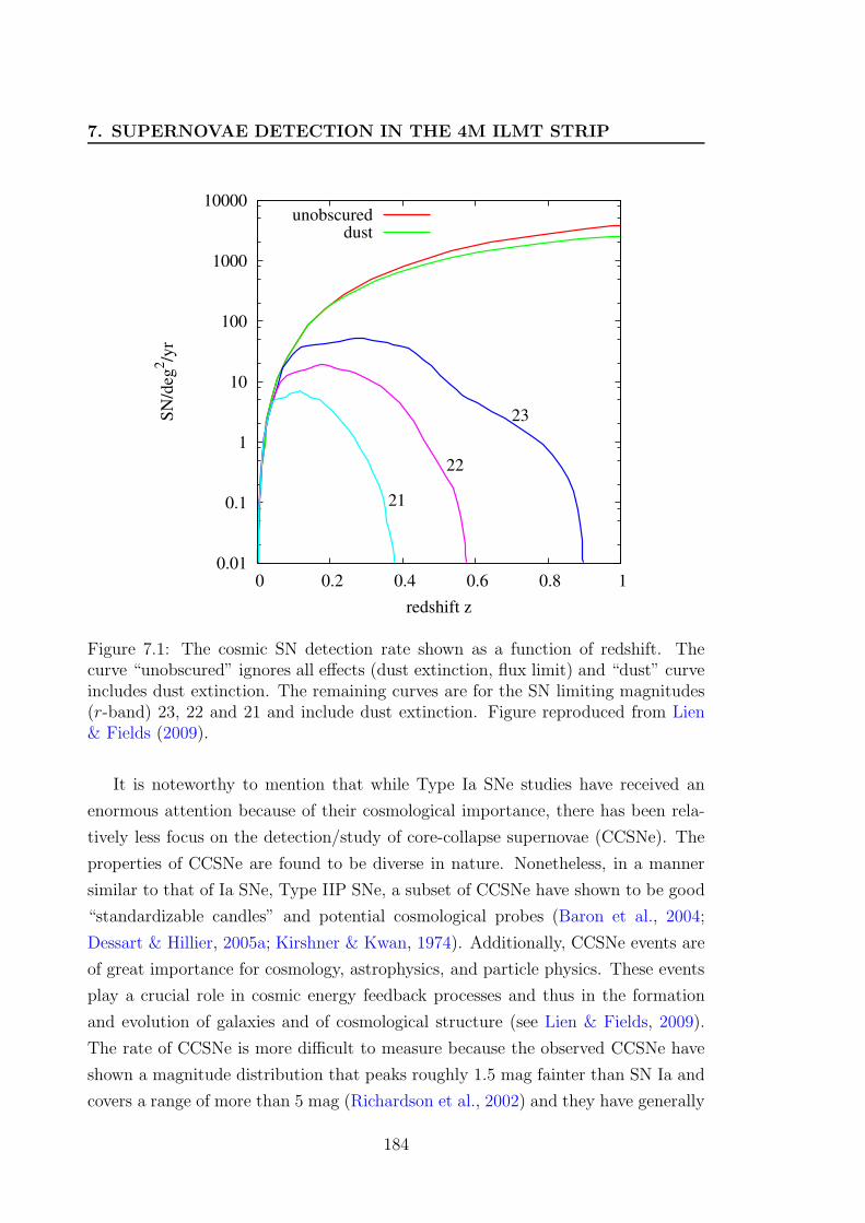
7. SUPERNOVAE DETECTION IN THE 4M ILMT STRIP
0.01
0.1
1
10
100
1000
10000
0 0.2 0.4 0.6 0.8 1
SN
/deg
2/y
r
redshift z
23
22
21
unobscureddust
Figure 7.1: The cosmic SN detection rate shown as a function of redshift. Thecurve “unobscured” ignores all effects (dust extinction, flux limit) and “dust” curveincludes dust extinction. The remaining curves are for the SN limiting magnitudes(r-band) 23, 22 and 21 and include dust extinction. Figure reproduced from Lien& Fields (2009).
It is noteworthy to mention that while Type Ia SNe studies have received an
enormous attention because of their cosmological importance, there has been rela-
tively less focus on the detection/study of core-collapse supernovae (CCSNe). The
properties of CCSNe are found to be diverse in nature. Nonetheless, in a manner
similar to that of Ia SNe, Type IIP SNe, a subset of CCSNe have shown to be good
“standardizable candles” and potential cosmological probes (Baron et al., 2004;
Dessart & Hillier, 2005a; Kirshner & Kwan, 1974). Additionally, CCSNe events are
of great importance for cosmology, astrophysics, and particle physics. These events
play a crucial role in cosmic energy feedback processes and thus in the formation
and evolution of galaxies and of cosmological structure (see Lien & Fields, 2009).
The rate of CCSNe is more difficult to measure because the observed CCSNe have
shown a magnitude distribution that peaks roughly 1.5 mag fainter than SN Ia and
covers a range of more than 5 mag (Richardson et al., 2002) and they have generally
184
7.2 Throughput and limiting magnitude of a telescope
been discovered in diverse types of galaxies.
7.2 Throughput and limiting magnitude of a tele-
scope
The scientific performance of an instrument depends on the maximization of its
throughput. The system throughput of an optical telescope (without a detector
like CCD) is generally expected to be about ∼60% for imaging mode. The expected
counts (Ne) from a star of certain brightness can be estimated considering the trans-
mission coefficients from the mirrors, filters, CCD glass, sky, extinction, quantum
efficiency of the CCD chip etc. using the formula given in McLean 1989, see also
Mayya (1991):
Ne = 3.95× 10¹¹ D2 λn ∆λn F n0 10−0.4mAF η (7.1)
where D is the diameter of the telescope, λn and ∆λn are the effective wavelength
and bandwidth of the filters, F n0 is the flux density from a star of magnitude 0 at
the wavelength λn above the Earth atmosphere, AF is the fractional reflecting area
of the mirror surface and η is the efficiency of the system.
Assuming that each optical photon will be able to produce a corresponding
photoelectron, the full well capacity of the required CCD pixel could be estimated
by assuming a certain integration time for a star of a known brightness. Also, if the
sky brightness is known, for a given CCD and the parameters like pixel size, dark
current, read out noise, we can also calculate the sky counts and the underlying
noise.
N =√
(Ne et + Se et np +Dc et np +R2n np) (7.2)
here Ne indicates the number of electrons (per sec), et the exposure time (sec),
Se the sky electrons, np the number of pixels, Dc the dark current (e−/pix/sec), Rn
the read out noise.
The signal-to-noise ratio can also be calculated for the stars of different bright-
ness (McLean, 1989).
185
7. SUPERNOVAE DETECTION IN THE 4M ILMT STRIP
Signal/Noise =
(
Ne × etN
)
. (7.3)
The CCD readout noise is Gaussian while the star counts, dark counts are Pois-
son in nature. The aperture to calculate the star light is considered as circular.
For the calculations, the FWHM is considered as 1.5 arcsec, nearly equal to the
median seeing at Devasthal. The optimal aperture is considered to be 1 × FWHM
(see Howell, 1989, 2000).
We can also estimate the corresponding error in the magnitude estimation by
knowing the value of the signal-to-noise ratio (Deep et al., 2011).
σmag = 2.5× log10(1 + 1/(Signal/Noise)). (7.4)
Estimation of the ILMT limiting magnitudes
We have estimated the limiting magnitudes of the ILMT for different filters (g′,
r′ and i′) using the previous equations. The various parameters used for these
estimations are listed in Table 7.1. The limiting magnitudes for different filters
are overplotted in Fig. 7.2 with different symbols. It is obvious from this figure
that with an exposure time of 102 sec, the limiting magnitudes are ∼21.4, ∼22.2
and ∼22.8 for the i′, r′ and g′ filters, respectively. Furthermore, since during each
night the same strip of sky will pass over the telescope, successive night images
can be co-added. This will yield longer integration times. Therefore, we have also
estimated the limiting magnitudes for 306 sec (3 night images) exposure time, using
the same parameters. The estimated magnitude limit improves to ∼22.0, ∼22.8
and ∼23.4 mag for g′, r′ and i′ filters, respectively. The co-addition technique is not
limited only for 3 nights but it can also be applied for several night imaging data.
Consequently, we may reach still fainter magnitude levels. It is also described in
Borra (2001a,b, 2003).
7.3 Area and accessible volume of the ILMT strip
Pointing towards zenith, the ILMT field-of-view (FOV) is centered at the Devasthal
observatory latitude which is 29.3611 N. The ILMT FOV is 27’ by 27’. As the
186
7.3 Area and accessible volume of the ILMT strip
Table 7.1: Different parameters used to calculate the ILMT limiting magnitude. Seealso Finet (2013).
Diameter 4.0mFraction of reflecting area 0.95Reflectivity 0.77Mylar transmission 0.80FWHM 1.5”CCD pixel size 0.4”/pixelCCD dark noise 0.00083 e−/pixel/secCCD readout noise 5.0 e−
Wavelength (g′, r′, i′) 4750, 6250, 7630 AWavelength FWHM (g′, r′, i′) 1450, 1500, 1500 AExtinction (∼ g′,∼ r′,∼ i′) 0.21, 0.13, 0.08 magSky mag (∼ g′,∼ r′,∼ i′) 21.3, 20.5, 18.9 mag/arcsec2
CCD quantum efficiency (g′, r′, i′) 0.70, 0.91, 0.91Filter transmission (g′, r′, i′) 0.92, 0.95, 0.95
Earth rotates, the ILMT will access a strip of sky. We can estimate the total solid
angle ΩILMT accessible by the ILMT using the following relation (see Finet, 2013):
ΩILMT =
∫ 2π
0
∫ +δ
−δ
cos(δ) dδ dα (7.5)
The sky coverage comes out to be 141.2 square degrees. Here α and δ denote
the right ascension and declination, respectively in radians. δ± = δILMT ±∆ILMT/2
represent the declinations of the accessible strip borders. ∆ILMT = 27 arcmin.
The area accessible with the ILMT is indicated in Fig. 5.3. It should be noted
that considering the site advantage, out of 141.2 square degrees of sky, ∼72 square
degrees will belong to high galactic latitude (|b| > 30). In this high galactic region
detection of fainter and more distant objects (e.g. SNe, galaxies, quasars,...) will
be possible (see Finet, 2013; Magette, 2010; Surdej et al., 2006).
For different redshifts, we calculated the volume of sky expected to be covered
by the ILMT using the formula given in Taylor et al. (2014, see eq. 7).
V =1
3∆θ∆φ(D3
z2 −D3z1) (7.6)
whereDz1 andDz2 are the co-moving distances at redshift z1 and z2, respectively.
∆θ is the declination range (0.45) and ∆φ is the right ascension (R.A.) range –50
187
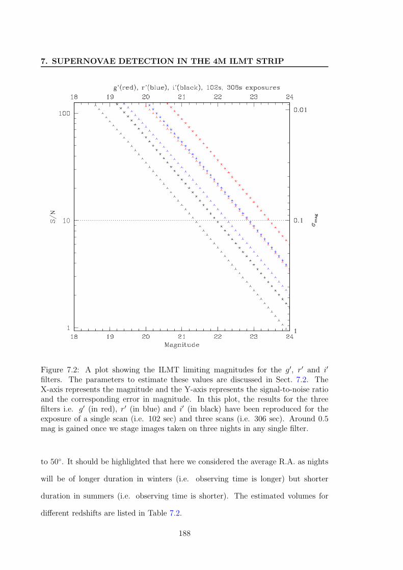
7. SUPERNOVAE DETECTION IN THE 4M ILMT STRIP
Figure 7.2: A plot showing the ILMT limiting magnitudes for the g′, r′ and i′
filters. The parameters to estimate these values are discussed in Sect. 7.2. TheX-axis represents the magnitude and the Y-axis represents the signal-to-noise ratioand the corresponding error in magnitude. In this plot, the results for the threefilters i.e. g′ (in red), r′ (in blue) and i′ (in black) have been reproduced for theexposure of a single scan (i.e. 102 sec) and three scans (i.e. 306 sec). Around 0.5mag is gained once we stage images taken on three nights in any single filter.
to 50. It should be highlighted that here we considered the average R.A. as nights
will be of longer duration in winters (i.e. observing time is longer) but shorter
duration in summers (i.e. observing time is shorter). The estimated volumes for
different redshifts are listed in Table 7.2.
188
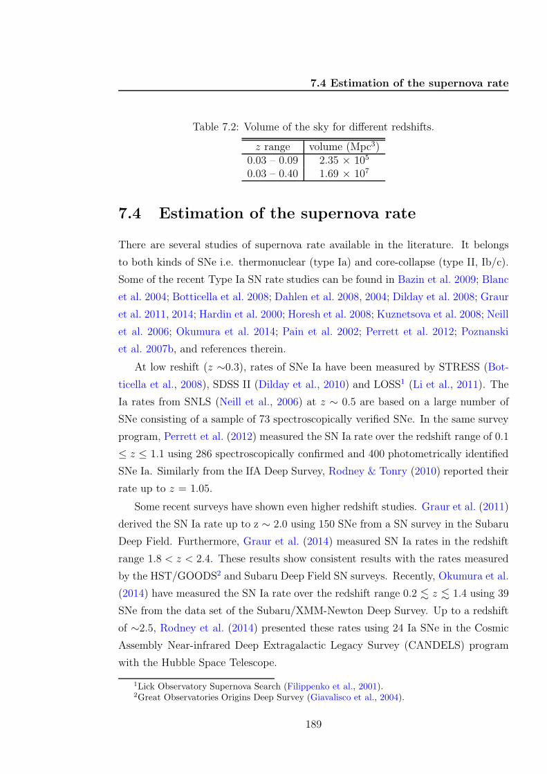
7.4 Estimation of the supernova rate
Table 7.2: Volume of the sky for different redshifts.
z range volume (Mpc3)0.03 – 0.09 2.35 × 10⁵
0.03 – 0.40 1.69 × 10⁷
7.4 Estimation of the supernova rate
There are several studies of supernova rate available in the literature. It belongs
to both kinds of SNe i.e. thermonuclear (type Ia) and core-collapse (type II, Ib/c).
Some of the recent Type Ia SN rate studies can be found in Bazin et al. 2009; Blanc
et al. 2004; Botticella et al. 2008; Dahlen et al. 2008, 2004; Dilday et al. 2008; Graur
et al. 2011, 2014; Hardin et al. 2000; Horesh et al. 2008; Kuznetsova et al. 2008; Neill
et al. 2006; Okumura et al. 2014; Pain et al. 2002; Perrett et al. 2012; Poznanski
et al. 2007b, and references therein.
At low reshift (z ∼0.3), rates of SNe Ia have been measured by STRESS (Bot-
ticella et al., 2008), SDSS II (Dilday et al., 2010) and LOSS1 (Li et al., 2011). The
Ia rates from SNLS (Neill et al., 2006) at z ∼ 0.5 are based on a large number of
SNe consisting of a sample of 73 spectroscopically verified SNe. In the same survey
program, Perrett et al. (2012) measured the SN Ia rate over the redshift range of 0.1
≤ z ≤ 1.1 using 286 spectroscopically confirmed and 400 photometrically identified
SNe Ia. Similarly from the IfA Deep Survey, Rodney & Tonry (2010) reported their
rate up to z = 1.05.
Some recent surveys have shown even higher redshift studies. Graur et al. (2011)
derived the SN Ia rate up to z ∼ 2.0 using 150 SNe from a SN survey in the Subaru
Deep Field. Furthermore, Graur et al. (2014) measured SN Ia rates in the redshift
range 1.8 < z < 2.4. These results show consistent results with the rates measured
by the HST/GOODS2 and Subaru Deep Field SN surveys. Recently, Okumura et al.
(2014) have measured the SN Ia rate over the redshift range 0.2 . z . 1.4 using 39
SNe from the data set of the Subaru/XMM-Newton Deep Survey. Up to a redshift
of ∼2.5, Rodney et al. (2014) presented these rates using 24 Ia SNe in the Cosmic
Assembly Near-infrared Deep Extragalactic Legacy Survey (CANDELS) program
with the Hubble Space Telescope.
1Lick Observatory Supernova Search (Filippenko et al., 2001).2Great Observatories Origins Deep Survey (Giavalisco et al., 2004).
189
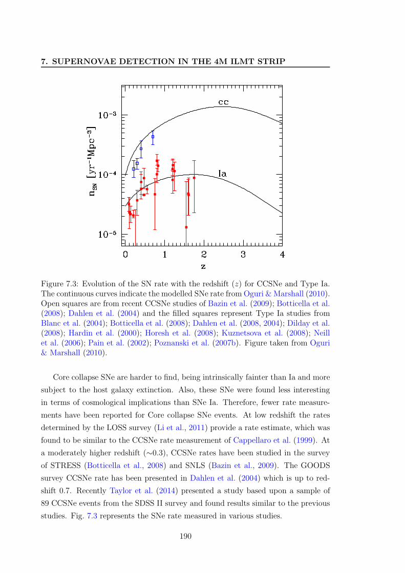
7. SUPERNOVAE DETECTION IN THE 4M ILMT STRIP
Figure 7.3: Evolution of the SN rate with the redshift (z) for CCSNe and Type Ia.The continuous curves indicate the modelled SNe rate from Oguri & Marshall (2010).Open squares are from recent CCSNe studies of Bazin et al. (2009); Botticella et al.(2008); Dahlen et al. (2004) and the filled squares represent Type Ia studies fromBlanc et al. (2004); Botticella et al. (2008); Dahlen et al. (2008, 2004); Dilday et al.(2008); Hardin et al. (2000); Horesh et al. (2008); Kuznetsova et al. (2008); Neillet al. (2006); Pain et al. (2002); Poznanski et al. (2007b). Figure taken from Oguri& Marshall (2010).
Core collapse SNe are harder to find, being intrinsically fainter than Ia and more
subject to the host galaxy extinction. Also, these SNe were found less interesting
in terms of cosmological implications than SNe Ia. Therefore, fewer rate measure-
ments have been reported for Core collapse SNe events. At low redshift the rates
determined by the LOSS survey (Li et al., 2011) provide a rate estimate, which was
found to be similar to the CCSNe rate measurement of Cappellaro et al. (1999). At
a moderately higher redshift (∼0.3), CCSNe rates have been studied in the survey
of STRESS (Botticella et al., 2008) and SNLS (Bazin et al., 2009). The GOODS
survey CCSNe rate has been presented in Dahlen et al. (2004) which is up to red-
shift 0.7. Recently Taylor et al. (2014) presented a study based upon a sample of
89 CCSNe events from the SDSS II survey and found results similar to the previous
studies. Fig. 7.3 represents the SNe rate measured in various studies.
190
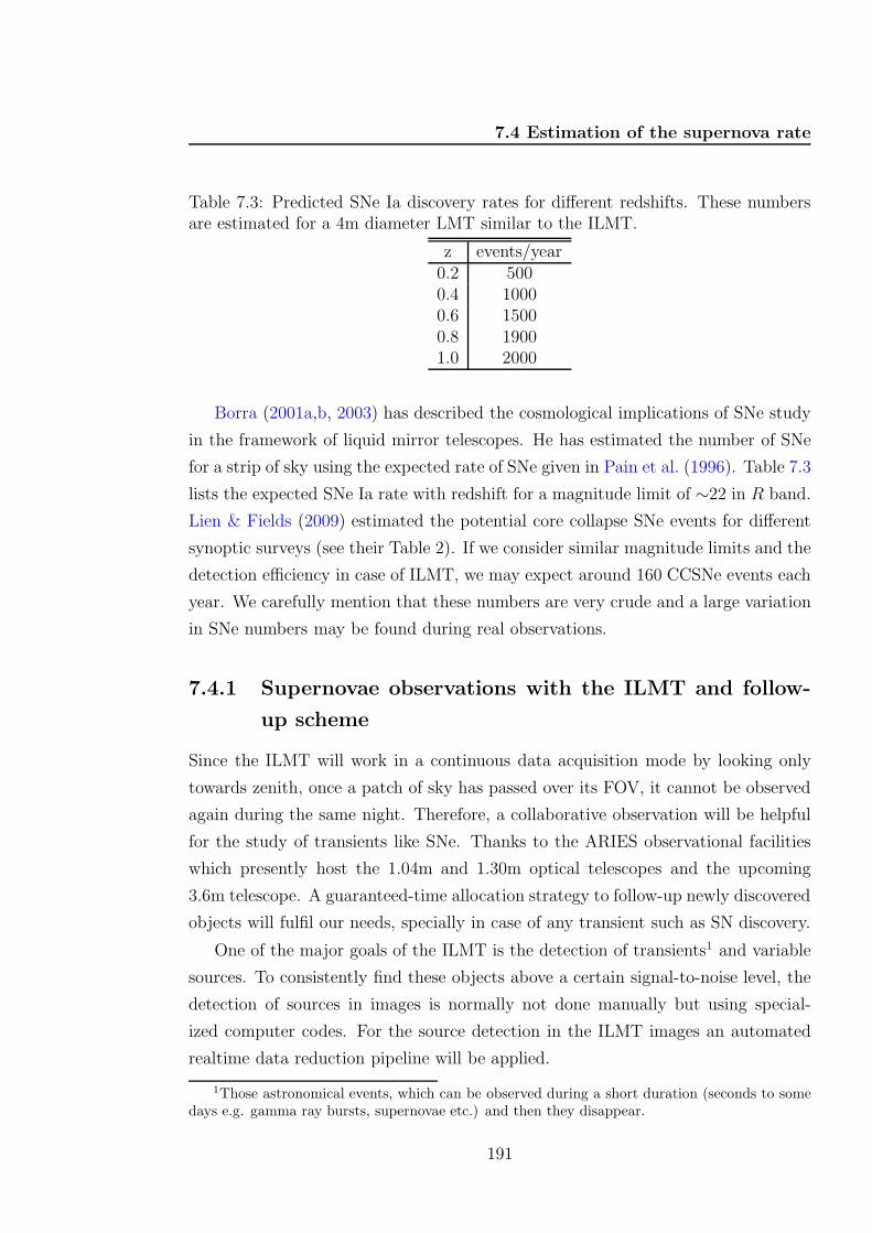
7.4 Estimation of the supernova rate
Table 7.3: Predicted SNe Ia discovery rates for different redshifts. These numbersare estimated for a 4m diameter LMT similar to the ILMT.
z events/year0.2 5000.4 10000.6 15000.8 19001.0 2000
Borra (2001a,b, 2003) has described the cosmological implications of SNe study
in the framework of liquid mirror telescopes. He has estimated the number of SNe
for a strip of sky using the expected rate of SNe given in Pain et al. (1996). Table 7.3
lists the expected SNe Ia rate with redshift for a magnitude limit of ∼22 in R band.
Lien & Fields (2009) estimated the potential core collapse SNe events for different
synoptic surveys (see their Table 2). If we consider similar magnitude limits and the
detection efficiency in case of ILMT, we may expect around 160 CCSNe events each
year. We carefully mention that these numbers are very crude and a large variation
in SNe numbers may be found during real observations.
7.4.1 Supernovae observations with the ILMT and follow-
up scheme
Since the ILMT will work in a continuous data acquisition mode by looking only
towards zenith, once a patch of sky has passed over its FOV, it cannot be observed
again during the same night. Therefore, a collaborative observation will be helpful
for the study of transients like SNe. Thanks to the ARIES observational facilities
which presently host the 1.04m and 1.30m optical telescopes and the upcoming
3.6m telescope. A guaranteed-time allocation strategy to follow-up newly discovered
objects will fulfil our needs, specially in case of any transient such as SN discovery.
One of the major goals of the ILMT is the detection of transients1 and variable
sources. To consistently find these objects above a certain signal-to-noise level, the
detection of sources in images is normally not done manually but using special-
ized computer codes. For the source detection in the ILMT images an automated
realtime data reduction pipeline will be applied.
1Those astronomical events, which can be observed during a short duration (seconds to somedays e.g. gamma ray bursts, supernovae etc.) and then they disappear.
191
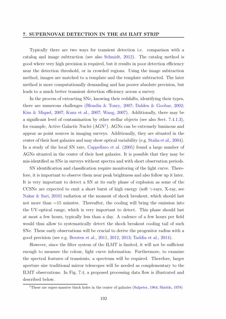
7. SUPERNOVAE DETECTION IN THE 4M ILMT STRIP
Typically there are two ways for transient detection i.e. comparison with a
catalog and image subtraction (see also Schmidt, 2012). The catalog method is
good where very high precision is required, but it results in poor detection efficiency
near the detection threshold, or in crowded regions. Using the image subtraction
method, images are matched to a template and the template subtracted. The later
method is more computationally demanding and has poorer absolute precision, but
leads to a much better transient detection efficiency across a survey.
In the process of extracting SNe, knowing their redshifts, identifying their types,
there are numerous challenges (Blondin & Tonry, 2007; Dahlen & Goobar, 2002;
Kim & Miquel, 2007; Kunz et al., 2007; Wang, 2007). Additionally, there may be
a significant level of contamination by other stellar objects (see also Sect. 7.4.1.3),
for example, Active Galactic Nuclei (AGN1). AGNs can be extremely luminous and
appear as point sources in imaging surveys. Additionally, they are situated in the
center of their host galaxies and may show optical variability (e.g. Stalin et al., 2004).
In a study of the local SN rate, Cappellaro et al. (2005) found a large number of
AGNs situated in the center of their host galaxies. It is possible that they may be
mis-identified as SNe in surveys without spectra and with short observation periods.
SN identification and classification require monitoring of the light curve. There-
fore, it is important to observe them near peak brightness and also follow up it later.
It is very important to detect a SN at its early phase of explosion as some of the
CCSNe are expected to emit a short burst of high energy (soft γ-rays, X-ray, see
Nakar & Sari, 2010) radiation at the moment of shock breakout, which should last
not more than ∼15 minutes. Thereafter, the cooling will bring the emission into
the UV-optical range, which is very important to detect. This phase should last
at most a few hours, typically less than a day. A cadence of a few hours per field
would thus allow to systematically detect the shock breakout cooling tail of such
SNe. These early observations will be crucial to derive the progenitor radius with a
good precision (see e.g. Bersten et al., 2011, 2012, 2013; Taddia et al., 2014).
However, since the filter system of the ILMT is limited, it will not be sufficient
enough to measure the colour, light curve information. Furthermore, to examine
the spectral features of transients, a spectrum will be required. Therefore, larger
aperture size traditional mirror telescopes will be needed as complementary to the
ILMT observations. In Fig. 7.4, a proposed processing data flow is illustrated and
described below.
1These are super-massive black holes in the center of galaxies (Salpeter, 1964; Shields, 1978)
192
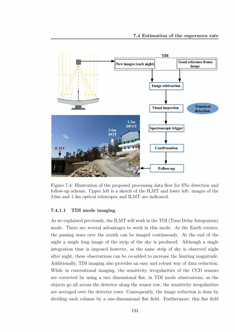
7.4 Estimation of the supernova rate
Figure 7.4: Illustration of the proposed processing data flow for SNe detection andfollow-up scheme. Upper left is a sketch of the ILMT and lower left: images of the3.6m and 1.3m optical telescopes and ILMT are indicated.
7.4.1.1 TDI mode imaging
As we explained previously, the ILMT will work in the TDI (Time Delay Integration)
mode. There are several advantages to work in this mode. As the Earth rotates,
the passing stars over the zenith can be imaged continuously. At the end of the
night a single long image of the strip of the sky is produced. Although a single
integration time is imposed however, as the same strip of sky is observed night
after night, these observations can be co-added to increase the limiting magnitude.
Additionally, TDI imaging also provides an easy and robust way of data reduction.
While in conventional imaging, the sensitivity irregularities of the CCD sensors
are corrected by using a two dimensional flat, in TDI mode observations, as the
objects go all across the detector along the sensor row, the sensitivity irregularities
are averaged over the detector rows. Consequently, the image reduction is done by
dividing each column by a one-dimensional flat field. Furthermore, this flat field
193
7. SUPERNOVAE DETECTION IN THE 4M ILMT STRIP
Figure 7.5: Image subtraction. Right panel: Galaxy UGC 01626 image withSN 2011fu. The SN can be seen in one of the spiral arms indicated by a circle.Left panel: Subtracted image where the SN is clearly visible without galaxy con-tamination.
can be directly estimated from the scientific data, contrary to what is done during
conventional imaging where flat field images must be taken before and/or after
scientific imaging. In this way precious telescope time is saved.
7.4.1.2 Image subtraction
Discovering a SN is not an easy task as in most cases the SN light will be a small
part of light measured from the galaxy. Furthermore, for high redshift galaxies, the
galaxies themselves will not be fully resolved by ground based observations so a SN
will be even less distinct and can be easily missed when looking in the individual
search epoch images.
However, in case of the ILMT since the same strip of sky will pass over the tele-
scope each night, observations will be performed under the best seeing conditions
by looking at the zenith during each clear night. Then previous night images or
a good reference image will be subtracted from the search night images using the
Optimal Image Subtraction (OIS) technique presented in Alard & Lupton (1998)
and further refined in Alard (ISIS, 2000). This method of image subtraction has
already been used to detect SNe in many projects (e.g. Botticella et al., 2008; Cap-
pellaro et al., 2005; Poznanski et al., 2007b; Wood-Vasey et al., 2007). In Fig. 7.5,
we demonstrate one example of the image subtraction technique.
194
7.4 Estimation of the supernova rate
7.4.1.3 Transient detection and possible contamination
The subtracted images may consist of astrophysical and non-astrophysical sources.
However, it has been found that in other transient surveys which use image sub-
traction techniques, that non-astrophysical sources always engulf the real sources
(e.g. Bloom et al., 2012; Brink et al., 2013). Non-astrophysical sources include cos-
mic rays that are not removed by cosmic ray removal software, extended features
around very bright saturated stars, and bad subtractions due to a mis-alignment of
the images. To remove these false detections, we must exclude the sources around
the bright, saturated stars and at the edges of the images.
Variable stars, quasars, active galaxies and moving objects also contaminate
the data. We can cross-match the detected object catalog with quasar and AGN
catalogs (Paris et al., 2014; Veron-Cetty & Veron, 2010). Variable stars can be
verified from SIMBAD1. The proper motion of asteroids is larger so they will show
significant variation in their position and can be removed easily. Furthermore, the
solar system objects can be checked from the Minor Planet Checker2.
7.4.1.4 Further observations
The light curves, the absolute luminosity and the colour evolution of SNe have pro-
vided major insights into the supernova phenomenon. Furthermore, the temporal
evolution of the energy release by the SNe is one of the major sources of information
about the nature of these events. Therefore, obtaining multi-band light curve obser-
vations is very important. Through light curves it has been possible to distinguish
between progenitor models, infer some aspects of the progenitor evolution, measure
the power sources, detail the explosion models, and probe the local environment of
the supernova explosions (Leibundgut & Suntzeff, 2003). The spectrum of a super-
nova contains a wealth of information about the composition and distribution of
elements in the exploding star. It also contains information on its redshift and age
(defined as the number of days from maximum light in a given filter). It is very
important to launch follow-up (photometric and spectroscopic) observations right
after the discovery of any transient.
1http://simbad.u-strasbg.fr/simbad/2http://scully.cfa.harvard.edu/cgi-bin/checkmp.cgi
195
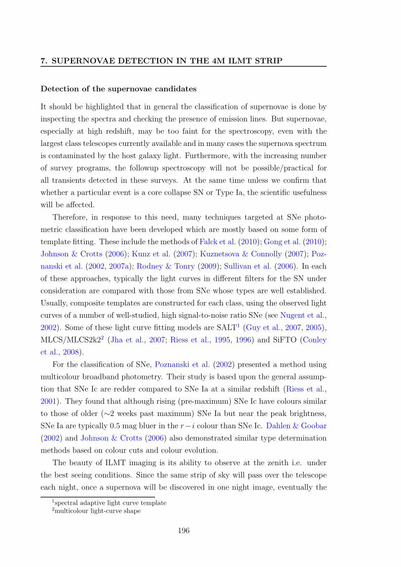
7. SUPERNOVAE DETECTION IN THE 4M ILMT STRIP
Detection of the supernovae candidates
It should be highlighted that in general the classification of supernovae is done by
inspecting the spectra and checking the presence of emission lines. But supernovae,
especially at high redshift, may be too faint for the spectroscopy, even with the
largest class telescopes currently available and in many cases the supernova spectrum
is contaminated by the host galaxy light. Furthermore, with the increasing number
of survey programs, the followup spectroscopy will not be possible/practical for
all transients detected in these surveys. At the same time unless we confirm that
whether a particular event is a core collapse SN or Type Ia, the scientific usefulness
will be affected.
Therefore, in response to this need, many techniques targeted at SNe photo-
metric classification have been developed which are mostly based on some form of
template fitting. These include the methods of Falck et al. (2010); Gong et al. (2010);
Johnson & Crotts (2006); Kunz et al. (2007); Kuznetsova & Connolly (2007); Poz-
nanski et al. (2002, 2007a); Rodney & Tonry (2009); Sullivan et al. (2006). In each
of these approaches, typically the light curves in different filters for the SN under
consideration are compared with those from SNe whose types are well established.
Usually, composite templates are constructed for each class, using the observed light
curves of a number of well-studied, high signal-to-noise ratio SNe (see Nugent et al.,
2002). Some of these light curve fitting models are SALT1 (Guy et al., 2007, 2005),
MLCS/MLCS2k22 (Jha et al., 2007; Riess et al., 1995, 1996) and SiFTO (Conley
et al., 2008).
For the classification of SNe, Poznanski et al. (2002) presented a method using
multicolour broadband photometry. Their study is based upon the general assump-
tion that SNe Ic are redder compared to SNe Ia at a similar redshift (Riess et al.,
2001). They found that although rising (pre-maximum) SNe Ic have colours similar
to those of older (∼2 weeks past maximum) SNe Ia but near the peak brightness,
SNe Ia are typically 0.5 mag bluer in the r−i colour than SNe Ic. Dahlen & Goobar
(2002) and Johnson & Crotts (2006) also demonstrated similar type determination
methods based on colour cuts and colour evolution.
The beauty of ILMT imaging is its ability to observe at the zenith i.e. under
the best seeing conditions. Since the same strip of sky will pass over the telescope
each night, once a supernova will be discovered in one night image, eventually the
1spectral adaptive light curve template2multicolour light-curve shape
196

7.4 Estimation of the supernova rate
same field will be observed again during the next nights. In this way a very good
sampling of data will be achieved to finally produce good sampled light curves in
different filters. If the ILMT observations could be performed in at least two filters
each night, the colour information or template fitting technique could be very much
useful to identify the supernova candidates for further followup.
Although a major drawback of the light curve fitting method is that its typing
determination is less accurate than the spectral method, it is much easier to obtain
photometry and construct light curves of faint SNe at high redshift in comparison
to obtaining spectra (see Melinder, 2011).
Spectroscopic trigger
Followup spectroscopy of a subset of events will be essential to calibrate the ac-
curacy of the photometric typing (and host redshifts). In particular, spectroscopy
will be invaluable in identifying and quantifying catastrophic failures in the typing
algorithms; on the basis of these it may be possible to refine the routines. As SNe
are random events i.e. there is no advance knowledge of where they will occur.
Therefore, it is not easy to obtain observing time in advance as in general the time
allocation is allotted on the basis of research proposals written about more than six
months in advance. Over that successful proposals are granted only a few nights
in a semester on bigger telescopes. Thanks to the upcoming 3.6m DOT telescope
situated near the ILMT site, it can be triggered in the target of opportunity ob-
servation mode in case of any transient like a SN is detected. Additionally, we can
collaborate with other existing facilities in India and world wide.
Confirmation
The individual emission/absorption lines in the spectra provide information about
the progenitor system and the new elements created in the explosion. Since the
classification of SNe is based on their optical spectra around maximum light (for a
review see Filippenko, 1997), therefore, for a rapid confirmation we can use available
SN classification codes e.g. GELATO1 and/or SNID2. The SNID tool is developed
to determine the type, redshift, and age of a SN, using a single spectrum. The
algorithm is based on the correlation techniques of Tonry & Davis (1979) and relies
on the comparison of an input spectrum with a database of high-S/N template
1GEneric cLAssification TOol https://gelato.tng.iac.es/2Supernova Identification http://people.lam.fr/blondin.stephane/software/snid/
197
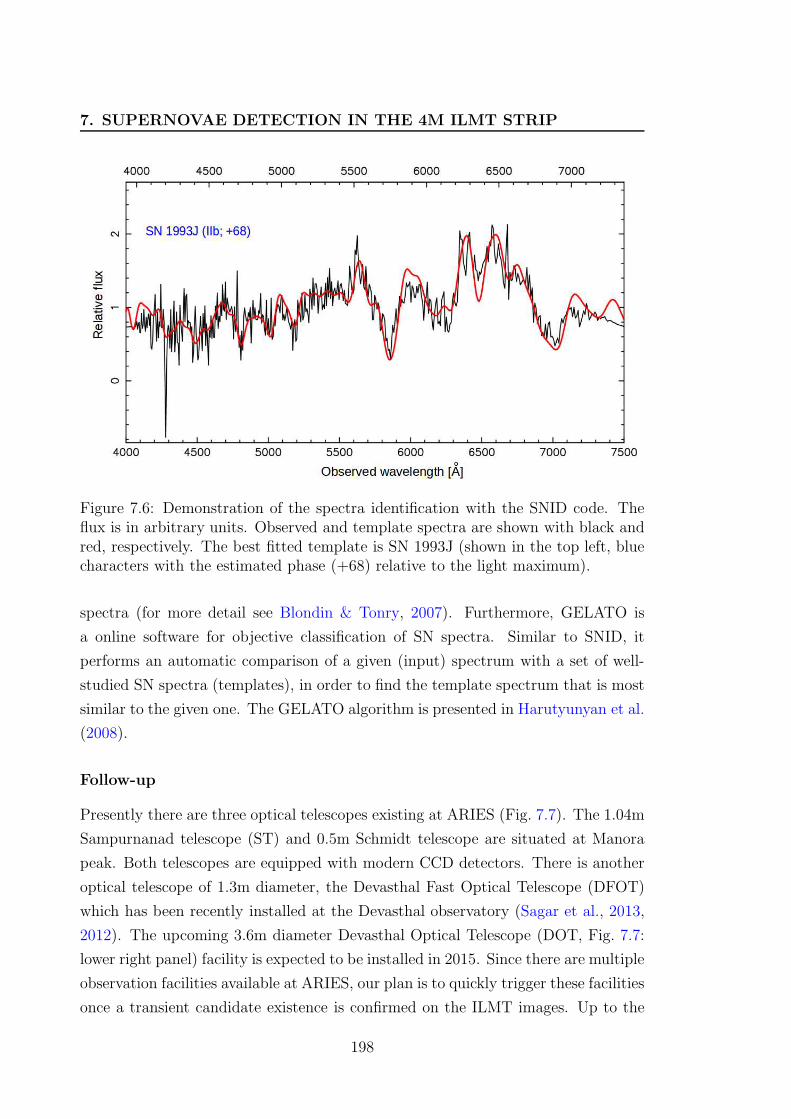
7. SUPERNOVAE DETECTION IN THE 4M ILMT STRIP
Figure 7.6: Demonstration of the spectra identification with the SNID code. Theflux is in arbitrary units. Observed and template spectra are shown with black andred, respectively. The best fitted template is SN 1993J (shown in the top left, bluecharacters with the estimated phase (+68) relative to the light maximum).
spectra (for more detail see Blondin & Tonry, 2007). Furthermore, GELATO is
a online software for objective classification of SN spectra. Similar to SNID, it
performs an automatic comparison of a given (input) spectrum with a set of well-
studied SN spectra (templates), in order to find the template spectrum that is most
similar to the given one. The GELATO algorithm is presented in Harutyunyan et al.
(2008).
Follow-up
Presently there are three optical telescopes existing at ARIES (Fig. 7.7). The 1.04m
Sampurnanad telescope (ST) and 0.5m Schmidt telescope are situated at Manora
peak. Both telescopes are equipped with modern CCD detectors. There is another
optical telescope of 1.3m diameter, the Devasthal Fast Optical Telescope (DFOT)
which has been recently installed at the Devasthal observatory (Sagar et al., 2013,
2012). The upcoming 3.6m diameter Devasthal Optical Telescope (DOT, Fig. 7.7:
lower right panel) facility is expected to be installed in 2015. Since there are multiple
observation facilities available at ARIES, our plan is to quickly trigger these facilities
once a transient candidate existence is confirmed on the ILMT images. Up to the
198
7.4 Estimation of the supernova rate
Figure 7.7: Present and upcoming facilities at ARIES, Manora peak and Devasthalobservatories. Top left and right panels: 1.04m ST and 0.5m Schmidt telescope,respectively. Bottom left and right panels are the images of the 1.3m DFOT andupcoming 3.6m DOT telescopes, respectively. These facilities will be used for thefollowup observations of the ILMT detected SNe and other transient events forphotometry and/or spectroscopy.
bright phase (∼19 magnitude) of SN , photometric observations will be performed
with different filters using small aperture telescopes and when it will become fainter
larger aperture telescopes (1.3m and 3.6m) will be utilized. However, spectroscopic
observations will be performed with the 3.6m DOT and other larger telescopes in
India and/or abroad.
199
7. SUPERNOVAE DETECTION IN THE 4M ILMT STRIP
7.5 Summary
We have presented the plans of SNe observations with the ILMT along with an
operational strategy and follow-up scheme. The ILMT survey will play an important
role is SNe detection with precise and unbiased imaging of a strip of sky at Devasthal.
During each night, the typical ILMT limiting magnitudes are 22.8, 22.2 and 21.4
mag in g′, r′ and i′ filters which can be obtained even deeper if we co-add the
successive night images. The multi-band and well sampled observations will enable
photometric type determination (by template fitting, colour information) of SNe
more accurately. Because of the tight link between SNe and star formation, the
ILMT with complementary observations and along with other sky surveys may
provide better measurements of the moderate red-shift history of the cosmic star-
formation rate.
Furthermore, the ILMT will provide an untargeted search with plentiful anony-
mous galaxies in each night images, which may allow us to construct a SN sample
without host-galaxy biases. By knowing the cosmic SN rate more precisely, the
cosmological uncertainties in the study of the wealth of observable properties of the
cosmic SN populations and their evolution with environment and redshift can be
removed. We are expecting to detect hundreds of Type Ia as well as core-collapse
SNe thanks to the ILMT survey over one year. New SNe discoveries and their light
curves could improve our knowledge on a variety of problems including cosmology
and SN physics.
200

Part IV
Conclusions and future prospects
201

Chapter 8
Conclusions and future prospects
This thesis is mainly based upon photometric and spectroscopic observations of
core-collapse supernovae (CCSNe), massive stars and activities related to the con-
struction and installation work of the 4m International Liquid Mirror Telescope
(ILMT) project. In addition to the photometric and spectroscopic observations, we
also performed polarimetric observations of a supernova to understand the effects
of the explosion from these highly energetic events on the ejected material.
The organization of this thesis is distributed into four parts having eight Chap-
ters. Part I gives a brief introduction about the massive stars and their evolution.
We briefly described various types of SNe along with their photometric, spectro-
scopic and polarimetric properties. Finally, we present the technological advance-
ment of liquid mirror telescopes and discussed their role in the context of the present
era of large astronomical telescopes.
In Part II “Study of supernovae and massive stars”, there are three Chapters.
We investigate the stellar content in the western part of the Carina nebula in Chap-
ter 2. The light curve and spectral properties of Type IIb SN 2011fu and broad
band polarimetric analysis of Type IIP SN 2012aw are presented in Chapters 3 and
4, respectively.
The low obscuration and proximity of the Carina nebula make it an ideal place
to study the ongoing star formation process and impact of massive stars on low-
mass stars in their surroundings. To investigate this process, we generated a new
catalog of the pre-main-sequence (PMS) stars in the Carina west (CrW) region and
studied their nature and spatial distribution. We also determined various parameters
(reddening, reddening law, age, mass), which are used further to estimate the initial
mass function (IMF) and K-band luminosity function (KLF) for the region under
study.
203
8. CONCLUSIONS AND FUTURE PROSPECTS
We obtained deep UBVRI Hα photometric data of the field situated to the west
of the main Carina nebula and centered on WR 22. Medium-resolution optical
spectroscopy of a subsample of X-ray selected objects along with archival data sets
from Chandra, XMM-Newton and 2MASS surveys were used for the present study.
Different sets of colour-colour and colour-magnitude diagrams are used to determine
reddening for the region and to identify young stellar objects (YSOs) and estimate
their age and mass.
Our spectroscopic results indicate that the majority of the X-ray sources are
late spectral type stars. The region shows a large amount of differential reddening
with minimum and maximum values of E(B−V ) as 0.25 and 1.1 mag, respectively.
Our analysis reveals that the total-to-selective absorption ratio RV is ∼3.7 ± 0.1,
suggesting an abnormal grain size in the observed region. We identified 467 YSO
candidates and studied their characteristics. The ages and masses of the 241 opti-
cally identified YSOs range from ∼0.1 to 10 Myr and ∼0.3 to 4.8 M⊙, respectively.
However, the majority of them are younger than 1 Myr and have masses below 2
M⊙.
The high mass star WR 22 does not seem to have contributed to the formation
of YSOs in the CrW region. The initial mass function slope, Γ, in this region
is found to be −1.13 ± 0.20 in the mass range of 0.5 < M/M⊙ < 4.8. The K-
band luminosity function slope (α) is estimated as 0.31 ± 0.01. We also performed
minimum spanning tree analysis of the YSOs in this region, which reveals that there
are at least ten YSO cores associated with the molecular cloud, and that leads to
an average core radius of 0.43 pc and a median branch length of 0.28 pc.
In Chapter 3, we have presented low-resolution spectroscopic and UBVRI broad-
band photometric investigations of the Type IIb supernova (SN) 2011fu, discovered
in the galaxy UGC 01626. The photometric follow-up of this event was initiated
within a few days after the explosion and covers a period of about 175 days. The
early-phase light curve shows a rise followed by a steep decay in all bands, and shares
properties very similar to those seen for SN 1993J, with a possible detection of the
adiabatic cooling phase. Modelling of the quasi-bolometric light curve suggests that
the progenitor had an extended (∼ 1 × 1013 cm), low-mass (∼ 0.1 M⊙) H-rich
envelope on top of a dense, compact (∼ 2 × 1011 cm), more massive (∼ 1.1 M⊙)
He-rich core. The nickel mass synthesized during the explosion was found to be ∼0.21 M⊙, slightly larger than that seen for the other Type IIb SNe. The spectral
modelling performed with SYNOW suggests that the early-phase line velocities of the H
204
and Fe ii features were ∼ 16000 km s−1 and ∼ 14000 km s−1, respectively. Then, the
velocities declined up to day +40 (after the explosion) and became nearly constant
at later epochs.
We have studied the polarimetric properties of the nearby (∼10 Mpc) Type II-
plateau SN 2012aw. Our analysis and results are presented in Chapter 4 which is
based upon the R-band polarimetric follow-up observations of this object. Starting
from ∼10 days after the SN explosion, these polarimetric observations cover ∼90
days (during the plateau phase) and are distributed over nine epochs. To charac-
terize the Milky Way interstellar polarization (ISPMW), we have observed 14 field
stars lying within a radius of 10 around the SN. We have also tried to subtract the
host galaxy dust polarization component assuming that the dust properties in the
host galaxy are similar to those observed for Galactic dust and the general magnetic
field follows the large scale structure of the spiral arms of the galaxy.
After correcting for the ISPMW, our analysis infers that SN 2012aw has a maxi-
mum polarization of 0.85% ± 0.08% and that the polarization angle does not show
much variation with a weighted mean value of ∼138. However, if both the ISPMW
and host galaxy polarization components are subtracted from the observed polar-
ization values of the SN, the maximum polarization of the SN becomes 0.68% ±0.08%. The distribution of the Q and U parameters appears to follow a loop like
structure. The evolution of the polarimetric light curve properties of this event is
also compared with other well studied core-collapse supernovae of similar type.
In Part III, we present our large efforts to make the liquid mirror technology
useful for the astronomical observations in the Northern hemisphere and in India
for the first time. We performed various experiments in the framework of building
the International Liquid Mirror Telescope. With a very simple structure, combined
with a CCD camera and an optical corrector, the ILMT will work in the time delay
integration imaging mode taking advantage of the best seeing conditions i.e. at the
zenith. This facility will be entirely dedicated and optimized for specific scientific
projects such as photometric and astrometric variability studies.
During the past few years, a number of experiments were executed to solve many
issues and technical problems related to the ILMT project. It includes spin casting
of the primary mirror, optical quality tests of the mercury surface and mylar film
experiments. The spin casting was performed to provide a pre-parabola shape of
the container so that later during the telescope operations it will require a smaller
amount of mercury which will finally lead to a better image quality.
205
8. CONCLUSIONS AND FUTURE PROSPECTS
To examine the optical quality of the mercury surface we performed experiments
using a laser source and a detector and verified the wavelets propagating on the
mercury surface. Measurements were carried out for different thicknesses of the
mercury layers. Our analysis indicates that there is absence of concentric wavelets
on the mirror however, signature of spiral wavelets was present. It is notable that
these experiments were limited due to sensitivity of the instrument, work place but,
it will be mandatory to repeat these experiments again when the ILMT will be
installed at site.
We have studied the influence of a mylar film by placing it on top of the tube of
the 1.04m Sampurnanad Telescope at ARIES, Nainital, in order to later suppress
the spiral waves induced by the rotation of the ILMT container. Our results infer
that use of this mylar film, diffuses ∼21% of the incident flux which is equivalent to
a loss of about 0.3 mag when imaging point-like celestial objects.
Along with the supernovae observations with the ILMT, we discussed its possible
scientific contributions. To detect the SNe candidates in the ILMT images, we
can co-add several night images and consequently deeper images will be obtained.
By applying the image subtraction technique we will be able to identify SN like
transients. The SNe type determination will be performed by spectral analysis and
also by the well established light curve template fitting methods. Further follow-
up observations will be done using ARIES as well as other observational facilities.
We are expecting to detect hundreds of supernovae every year thanks to the ILMT
observations.
Now the ILMT telescope is ready for its installation at Devasthal (Nainital,
India) observatory. For this purpose we have already procured several equipments
essential for the installation and smooth running of the ILMT facility. Some of
these items include air compressor, air receiver, dew point sensor, compressed air
membrane dryer, mercury vapor detectors, mercury vacuum cleaner, mercury safety
mask, etc. Many items are still to be procured in the near future such as computers,
storage devices, electrical UPS, automatic weather station, etc.
Future prospects
Major parts of the ILMT have already been shipped to India and safely reached at
the Devasthal observatory. Figures 8.1 and 8.2, respectively illustrate the proposed
layout of the ILMT location at Devasthal and the enclosure sketch. Along with
206
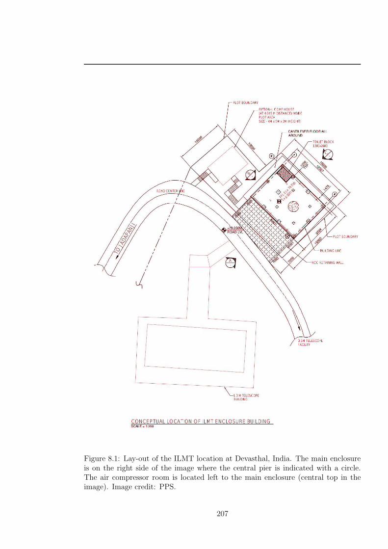
Figure 8.1: Lay-out of the ILMT location at Devasthal, India. The main enclosureis on the right side of the image where the central pier is indicated with a circle.The air compressor room is located left to the main enclosure (central top in theimage). Image credit: PPS.
207
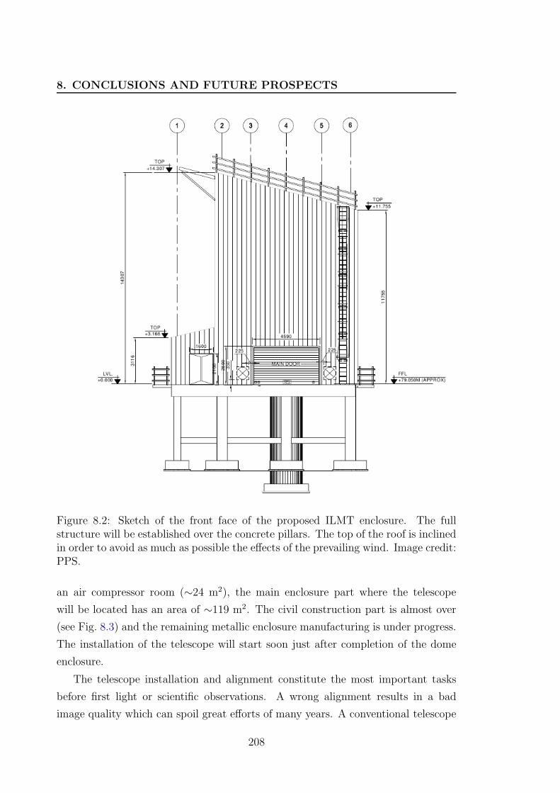
8. CONCLUSIONS AND FUTURE PROSPECTS
Figure 8.2: Sketch of the front face of the proposed ILMT enclosure. The fullstructure will be established over the concrete pillars. The top of the roof is inclinedin order to avoid as much as possible the effects of the prevailing wind. Image credit:PPS.
an air compressor room (∼24 m2), the main enclosure part where the telescope
will be located has an area of ∼119 m2. The civil construction part is almost over
(see Fig. 8.3) and the remaining metallic enclosure manufacturing is under progress.
The installation of the telescope will start soon just after completion of the dome
enclosure.
The telescope installation and alignment constitute the most important tasks
before first light or scientific observations. A wrong alignment results in a bad
image quality which can spoil great efforts of many years. A conventional telescope
208
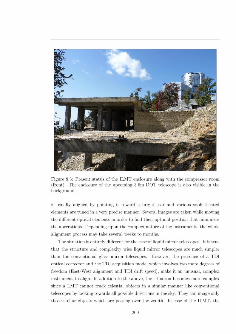
Figure 8.3: Present status of the ILMT enclosure along with the compressor room(front). The enclosure of the upcoming 3.6m DOT telescope is also visible in thebackground.
is usually aligned by pointing it toward a bright star and various sophisticated
elements are tuned in a very precise manner. Several images are taken while moving
the different optical elements in order to find their optimal position that minimizes
the aberrations. Depending upon the complex nature of the instruments, the whole
alignment process may take several weeks to months.
The situation is entirely different for the case of liquid mirror telescopes. It is true
that the structure and complexity wise liquid mirror telescopes are much simpler
than the conventional glass mirror telescopes. However, the presence of a TDI
optical corrector and the TDI acquisition mode, which involves two more degrees of
freedom (East-West alignment and TDI drift speed), make it an unusual, complex
instrument to align. In addition to the above, the situation becomes more complex
since a LMT cannot track celestial objects in a similar manner like conventional
telescopes by looking towards all possible directions in the sky. They can image only
those stellar objects which are passing over the zenith. In case of the ILMT, the
209
8. CONCLUSIONS AND FUTURE PROSPECTS
imaging instruments will be positioned at a height of around 8m above the rotating
mercury container and consequently the characterization and alignment will be a
difficult process. The astronomers involved in the large zenithal telescope project
which is presently the largest working liquid mirror facility are also associated with
the ILMT project. With their great expertise and dedicated team members, we are
extremely hopeful to install the ILMT facility in the near future and dedicate it to
the whole interested astronomical community.
An efficient software pipeline is necessary for the detection of transients and
real time observations. For a quick and responsive follow-up, image subtraction
technique must be included in the software so that each night, the previous night
images (or a good reference frame image) can be subtracted and spectroscopic trig-
ger can be requested immediately. Softwares have already been developed in due
course of time and preliminary processing tests have also been performed on it using
previously acquired TDI images with the 1.3m DFOT and a C-14” telescope. This
segment requires further involvement.
During night operation, the temperature inside the dome must be similar to the
temperature outside, within typically one C. Similar to a conventional telescope
enclosure building, it is necessary to design the ILMT enclosure so that the “dome”
seeing is minimized. Artificial sources of heat inside the mirror room, during the
day and, especially, at night must be minimized. The difference of temperature
inside and outside the dome shall in no time exceed 5C. Therefore, a rudimentary
air conditioning system is planned inside the ILMT dome in order to maintain a
temperature close to the external one at the beginning of the night.
Safety Related
Since mercury will be used to create the liquid mirror, safe handling of the mercury
constitutes one most important aspect during operations of the ILMT. In our ex-
periments for the surface quality verification over the mercury layer, we have learnt
many procedures for safe handling of the mercury. During our experiments we have
learnt how to properly operate mercury vapor detectors, mercury vacuum cleaner,
etc. We will follow all possible safety measures for the mercury vapor protection.
Four safety pillars just below the periphery of the bowl will be installed so that
if the mercury filled bowl accidently tilts in any direction, these pillars will prevent
it to tumble. To avoid the spread of mercury spilling, the floor of the enclosure base
210
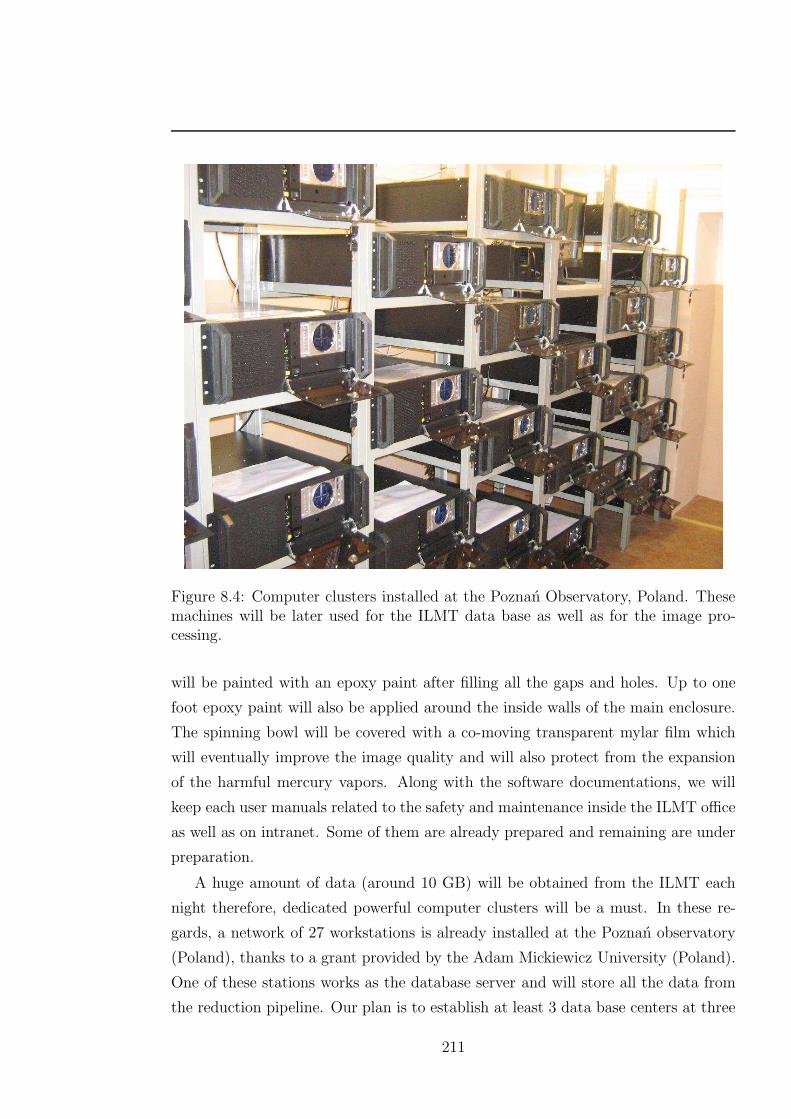
Figure 8.4: Computer clusters installed at the Poznan Observatory, Poland. Thesemachines will be later used for the ILMT data base as well as for the image pro-cessing.
will be painted with an epoxy paint after filling all the gaps and holes. Up to one
foot epoxy paint will also be applied around the inside walls of the main enclosure.
The spinning bowl will be covered with a co-moving transparent mylar film which
will eventually improve the image quality and will also protect from the expansion
of the harmful mercury vapors. Along with the software documentations, we will
keep each user manuals related to the safety and maintenance inside the ILMT office
as well as on intranet. Some of them are already prepared and remaining are under
preparation.
A huge amount of data (around 10 GB) will be obtained from the ILMT each
night therefore, dedicated powerful computer clusters will be a must. In these re-
gards, a network of 27 workstations is already installed at the Poznan observatory
(Poland), thanks to a grant provided by the Adam Mickiewicz University (Poland).
One of these stations works as the database server and will store all the data from
the reduction pipeline. Our plan is to establish at least 3 data base centers at three
211
8. CONCLUSIONS AND FUTURE PROSPECTS
different places. One base will be located at the Devasthal observatory, India. We
have to purchase large storage capacity devices along with high processing comput-
ers. We will also install a good quality video camera and an automatic weather
station for the continuous monitoring of the telescope and weather conditions, re-
spectively. A complete observatory control system is also planned in a later phase.
As obvious from Figs. 8.2 and 8.3, for cost saving purposes, the ILMT base has
been constructed on concrete pillars. There is ample space below the top portion.
We plan to manage this space for making offices, rest rooms and storage area for
the ILMT purposes.
The Devasthal observatory is soon going to host the 3.6m telescope (DOT)
which will be equipped with sophisticated instruments for low spectral resolution
observations and imaging capabilities in the visible and near-infrared bands. First
light of DOT is expected at the beginning of 2015. Once the 3.6m telescope will
be installed, it will be the largest telescope in Asia. Along with other science
goals, this telescope will be extremely useful for complementary observations of
the stellar objects detected with the ILMT (specially for the transients). We will
continue our follow-up programs (photometry, spectroscopy and polarimetry) to
study core collapse supernovae and other transients. The investigation of these
events may further tell us about some of the underlying question related to massive
star evolution.
212

Appendix
213
A. APPENDIX
Table A.1: List of the optically identified YSOs along with their derived
ages and masses. Error bars in magnitude and colour represent formal
internal (comparative) errors and do not include the colour transformation
and zero-point uncertainties. The numbers in the technique column indicate
the YSOs identified with different schemes (1: Spitzer identified sources, 2:
Hα sources, 3: CTTS, 4 Chandra sources, 5: XMM-Newton sources and 6:
Probable NIR excess)
ID α(J2000) δ(J2000) V ± σ (V − I)± σ Age ±σ Mass ±σ Technique
() () (mag) (mag) (Myrs) (M⊙) 1,2,3,4,5,6
(1) (2) (3) (4) (5) (6) (7) (8)
1 160.544858 -59.643538 12.316± 0.009 0.373± 0.018 0.9± 0.2 3.7± 0.2 1
2 160.586232 -59.898926 12.726± 0.011 0.211± 0.018 2.6± 2.1 4.8± 0.3 1
3 160.556561 -59.735036 13.079± 0.011 0.422± 0.014 1.4± 0.2 2.8± 0.3 1
4 159.827622 -59.759030 13.508± 0.006 0.677± 0.010 2.5± 0.4 2.0± 0.3 1
5 160.509158 -59.674841 13.527± 0.009 1.000± 0.014 1.4± 0.2 3.4± 0.3 1
6 160.773246 -59.888387 13.783± 0.014 0.890± 0.013 2.5± 0.4 2.7± 0.2 1
7 160.070496 -59.624432 14.001± 0.009 1.743± 0.010 0.1± 0.1 2.9± 0.1 1 2
8 160.314363 -59.631949 14.056± 0.037 0.899± 0.041 3.1± 0.5 2.5± 0.2 1
9 160.623657 -59.813984 14.220± 0.022 0.762± 0.016 5.0± 0.8 2.1± 0.3 1
10 160.580895 -59.847589 14.317± 0.020 1.014± 0.010 2.4± 0.4 2.8± 0.1 1
11 159.838120 -59.632839 14.342± 0.014 1.137± 0.010 1.2± 0.2 3.4± 0.1 2
12 160.705831 -59.767138 14.584± 0.024 0.923± 0.015 4.3± 0.6 2.1± 0.2 1
13 160.069977 -59.534346 14.720± 0.012 1.386± 0.007 0.3± 0.1 3.2± 0.1 5
14 160.671981 -59.794835 14.746± 0.018 0.965± 0.013 4.3± 0.7 2.2± 0.2 1
15 160.841873 -59.445595 14.917± 0.026 1.254± 0.041 0.8± 0.2 3.2± 0.1 1
16 160.101377 -59.846255 14.918± 0.015 1.184± 0.012 1.3± 0.3 3.0± 0.1 1 2
17 159.820572 -59.738407 15.208± 0.008 1.105± 0.012 3.0± 0.5 2.5± 0.1 2
18 160.214424 -59.622191 15.365± 0.008 1.332± 0.008 0.7± 0.1 2.8± 0.1 4 5
19 160.307350 -59.844427 15.454± 0.015 0.918± 0.014 8.6± 0.6 1.8± 0.1 1
20 160.642834 -59.703229 15.534± 0.012 2.053± 0.015 0.1± 0.1 1.2± 0.1 1 6
21 160.522348 -59.407467 15.739± 0.009 0.962± 0.007 9.3± 0.7 1.7± 0.1 3
22 160.700775 -59.424721 15.741± 0.010 1.622± 0.019 0.3± 0.1 1.6± 0.1 1 2 6
23 160.684442 -59.902335 15.749± 0.011 1.344± 0.012 0.9± 0.1 2.5± 0.1 1
24 160.206885 -59.738959 15.806± 0.009 1.207± 0.011 2.4± 0.5 2.4± 0.1 4
25 160.552671 -59.769595 15.833± 0.009 1.208± 0.007 2.3± 0.5 2.4± 0.1 1
26 160.187629 -59.842736 15.910± 0.017 1.974± 0.035 0.1± 0.1 1.0± 0.1 4
27 160.601418 -59.453720 15.936± 0.009 1.693± 0.012 0.3± 0.1 1.3± 0.1 4
28 160.190377 -59.720193 15.953± 0.009 1.517± 0.012 0.5± 0.1 1.8± 0.1 4
Continued on next page
214
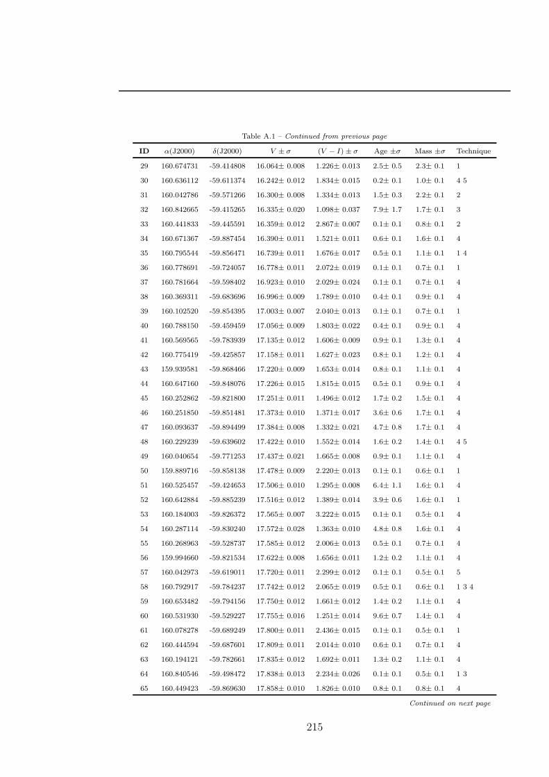
Table A.1 – Continued from previous page
ID α(J2000) δ(J2000) V ± σ (V − I)± σ Age ±σ Mass ±σ Technique
29 160.674731 -59.414808 16.064± 0.008 1.226± 0.013 2.5± 0.5 2.3± 0.1 1
30 160.636112 -59.611374 16.242± 0.012 1.834± 0.015 0.2± 0.1 1.0± 0.1 4 5
31 160.042786 -59.571266 16.300± 0.008 1.334± 0.013 1.5± 0.3 2.2± 0.1 2
32 160.842665 -59.415265 16.335± 0.020 1.098± 0.037 7.9± 1.7 1.7± 0.1 3
33 160.441833 -59.445591 16.359± 0.012 2.867± 0.007 0.1± 0.1 0.8± 0.1 2
34 160.671367 -59.887454 16.390± 0.011 1.521± 0.011 0.6± 0.1 1.6± 0.1 4
35 160.795544 -59.856471 16.739± 0.011 1.676± 0.017 0.5± 0.1 1.1± 0.1 1 4
36 160.778691 -59.724057 16.778± 0.011 2.072± 0.019 0.1± 0.1 0.7± 0.1 1
37 160.781664 -59.598402 16.923± 0.010 2.029± 0.024 0.1± 0.1 0.7± 0.1 4
38 160.369311 -59.683696 16.996± 0.009 1.789± 0.010 0.4± 0.1 0.9± 0.1 4
39 160.102520 -59.854395 17.003± 0.007 2.040± 0.013 0.1± 0.1 0.7± 0.1 1
40 160.788150 -59.459459 17.056± 0.009 1.803± 0.022 0.4± 0.1 0.9± 0.1 4
41 160.569565 -59.783939 17.135± 0.012 1.606± 0.009 0.9± 0.1 1.3± 0.1 4
42 160.775419 -59.425857 17.158± 0.011 1.627± 0.023 0.8± 0.1 1.2± 0.1 4
43 159.939581 -59.868466 17.220± 0.009 1.653± 0.014 0.8± 0.1 1.1± 0.1 4
44 160.647160 -59.848076 17.226± 0.015 1.815± 0.015 0.5± 0.1 0.9± 0.1 4
45 160.252862 -59.821800 17.251± 0.011 1.496± 0.012 1.7± 0.2 1.5± 0.1 4
46 160.251850 -59.851481 17.373± 0.010 1.371± 0.017 3.6± 0.6 1.7± 0.1 4
47 160.093637 -59.894499 17.384± 0.008 1.332± 0.021 4.7± 0.8 1.7± 0.1 4
48 160.229239 -59.639602 17.422± 0.010 1.552± 0.014 1.6± 0.2 1.4± 0.1 4 5
49 160.040654 -59.771253 17.437± 0.021 1.665± 0.008 0.9± 0.1 1.1± 0.1 4
50 159.889716 -59.858138 17.478± 0.009 2.220± 0.013 0.1± 0.1 0.6± 0.1 1
51 160.525457 -59.424653 17.506± 0.010 1.295± 0.008 6.4± 1.1 1.6± 0.1 4
52 160.642884 -59.885239 17.516± 0.012 1.389± 0.014 3.9± 0.6 1.6± 0.1 1
53 160.184003 -59.826372 17.565± 0.007 3.222± 0.015 0.1± 0.1 0.5± 0.1 4
54 160.287114 -59.830240 17.572± 0.028 1.363± 0.010 4.8± 0.8 1.6± 0.1 4
55 160.268963 -59.528737 17.585± 0.012 2.006± 0.013 0.5± 0.1 0.7± 0.1 4
56 159.994660 -59.821534 17.622± 0.008 1.656± 0.011 1.2± 0.2 1.1± 0.1 4
57 160.042973 -59.619011 17.720± 0.011 2.299± 0.012 0.1± 0.1 0.5± 0.1 5
58 160.792917 -59.784237 17.742± 0.012 2.065± 0.019 0.5± 0.1 0.6± 0.1 1 3 4
59 160.653482 -59.794156 17.750± 0.012 1.661± 0.012 1.4± 0.2 1.1± 0.1 4
60 160.531930 -59.529227 17.755± 0.016 1.251± 0.014 9.6± 0.7 1.4± 0.1 4
61 160.078278 -59.689249 17.800± 0.011 2.436± 0.015 0.1± 0.1 0.5± 0.1 1
62 160.444594 -59.687601 17.809± 0.011 2.014± 0.010 0.6± 0.1 0.7± 0.1 4
63 160.194121 -59.782661 17.835± 0.012 1.692± 0.011 1.3± 0.2 1.1± 0.1 4
64 160.840546 -59.498472 17.838± 0.013 2.234± 0.026 0.1± 0.1 0.5± 0.1 1 3
65 160.449423 -59.869630 17.858± 0.010 1.826± 0.010 0.8± 0.1 0.8± 0.1 4
Continued on next page
215

A. APPENDIX
Table A.1 – Continued from previous page
ID α(J2000) δ(J2000) V ± σ (V − I)± σ Age ±σ Mass ±σ Technique
66 160.808515 -59.826145 17.859± 0.013 1.667± 0.018 1.5± 0.2 1.1± 0.1 4
67 160.287467 -59.875219 17.869± 0.009 1.284± 0.008 9.3± 0.8 1.4± 0.1 4
68 160.181222 -59.914918 17.893± 0.009 1.955± 0.017 0.7± 0.1 0.7± 0.1 4
69 160.225893 -59.487413 17.906± 0.012 2.274± 0.015 0.1± 0.1 0.5± 0.1 4
70 160.666085 -59.465952 17.910± 0.010 2.446± 0.013 0.1± 0.1 0.5± 0.1 4
71 160.844931 -59.923162 17.926± 0.018 1.970± 0.016 0.7± 0.1 0.7± 0.1 1
72 160.141630 -59.751331 17.949± 0.008 1.601± 0.015 2.3± 0.4 1.2± 0.1 4
73 160.262140 -59.537419 17.970± 0.012 3.017± 0.011 0.1± 0.1 0.5± 0.1 4
74 160.347645 -59.859192 17.987± 0.010 1.707± 0.011 1.4± 0.2 1.0± 0.1 4
75 160.725325 -59.439794 18.003± 0.011 1.572± 0.016 2.9± 0.5 1.3± 0.1 4
76 160.360772 -59.499924 18.043± 0.011 2.634± 0.010 0.1± 0.1 0.5± 0.1 4
77 160.330190 -59.817178 18.086± 0.011 1.885± 0.009 0.9± 0.4 0.8± 1.4 4
78 160.735424 -59.704699 18.089± 0.014 1.998± 0.016 0.7± 0.1 0.7± 0.1 1 4
79 160.835598 -59.771479 18.095± 0.011 2.102± 0.021 0.6± 0.1 0.6± 0.1 4
80 160.620634 -59.742206 18.104± 0.015 1.391± 0.012 7.8± 1.1 1.4± 0.1 4
81 160.255001 -59.512966 18.109± 0.013 2.419± 0.013 0.1± 0.1 0.5± 0.1 4
82 160.594788 -59.655849 18.122± 0.016 1.324± 0.025 9.6± 0.6 1.3± 0.1 2
83 160.029372 -59.837043 18.128± 0.017 1.894± 0.018 0.9± 0.1 0.8± 0.1 1
84 160.231943 -59.830059 18.131± 0.013 2.192± 0.013 0.4± 0.1 0.5± 0.1 4
85 159.825531 -59.774998 18.143± 0.023 1.892± 0.014 0.9± 0.1 0.8± 0.1 2
86 160.517051 -59.802745 18.165± 0.014 2.389± 0.009 0.1± 0.1 0.5± 0.1 1
87 160.556738 -59.599388 18.204± 0.010 2.910± 0.013 0.1± 0.1 0.4± 0.1 1 3 4 5
88 160.655576 -59.847457 18.224± 0.014 2.149± 0.014 0.5± 0.1 0.5± 0.1 1 4
89 160.388550 -59.606377 18.232± 0.011 1.267± 0.011 10.0± 0.1 1.3± 0.1 2
90 160.218962 -59.583514 18.249± 0.013 1.990± 0.012 0.8± 0.1 0.7± 0.1 4
91 160.815765 -59.767838 18.366± 0.016 2.667± 0.020 0.1± 0.1 0.4± 0.1 1
92 160.667867 -59.861518 18.376± 0.018 2.603± 0.012 0.1± 0.1 0.4± 0.1 4
93 160.596668 -59.773186 18.391± 0.018 2.567± 0.018 0.1± 0.1 0.4± 0.1 1
94 159.965824 -59.779383 18.464± 0.011 2.424± 0.009 0.1± 0.1 0.4± 0.1 1
95 160.179539 -59.850030 18.488± 0.019 2.512± 0.012 0.1± 0.1 0.4± 0.1 4
96 160.213470 -59.779138 18.496± 0.011 1.473± 0.010 8.7± 1.0 1.2± 0.1 4
97 160.710477 -59.720586 18.506± 0.020 2.703± 0.017 0.1± 0.1 0.4± 0.1 1
98 160.750182 -59.452148 18.512± 0.014 1.908± 0.021 1.2± 0.1 0.8± 0.1 4
99 159.910376 -59.736938 18.524± 0.013 2.572± 0.010 0.1± 0.1 0.4± 0.1 1
100 160.811693 -59.705286 18.537± 0.019 1.777± 0.025 2.1± 0.3 0.9± 0.1 1
101 160.398495 -59.855793 18.544± 0.023 2.506± 0.012 0.1± 0.1 0.4± 0.1 4
102 159.942832 -59.605503 18.544± 0.017 5.495± 0.007 0.1± 0.1 0.3± 0.1 3
Continued on next page
216
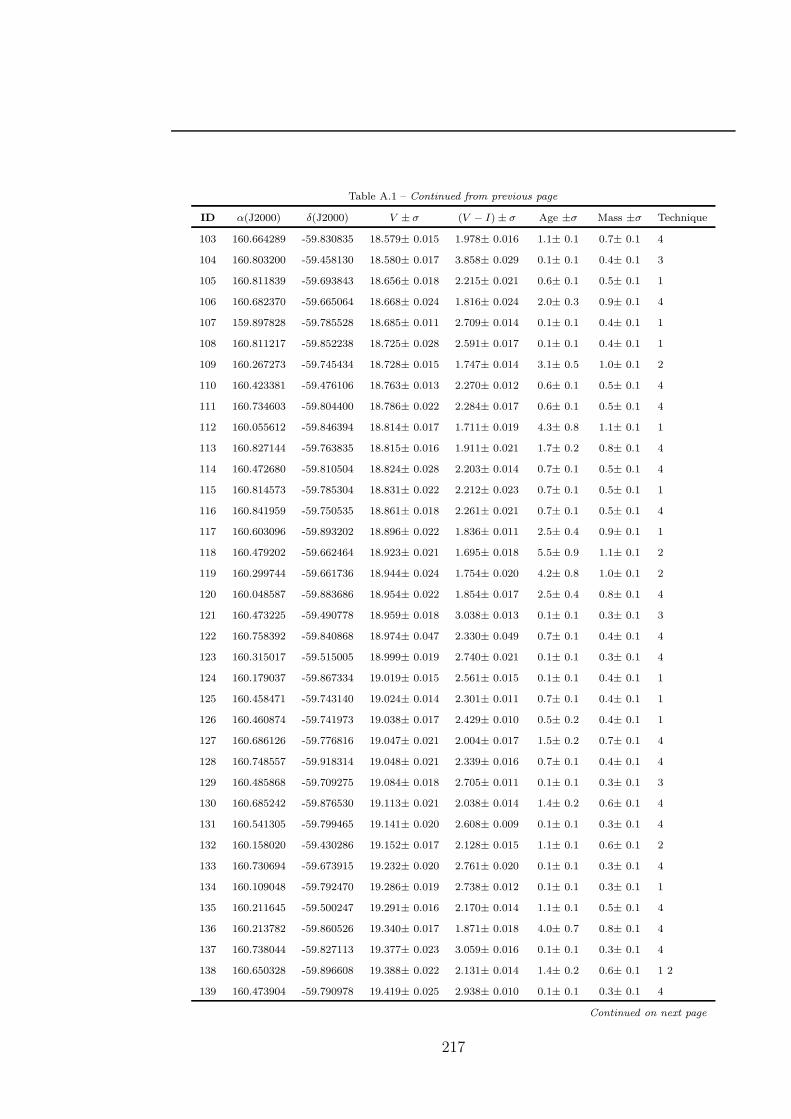
Table A.1 – Continued from previous page
ID α(J2000) δ(J2000) V ± σ (V − I)± σ Age ±σ Mass ±σ Technique
103 160.664289 -59.830835 18.579± 0.015 1.978± 0.016 1.1± 0.1 0.7± 0.1 4
104 160.803200 -59.458130 18.580± 0.017 3.858± 0.029 0.1± 0.1 0.4± 0.1 3
105 160.811839 -59.693843 18.656± 0.018 2.215± 0.021 0.6± 0.1 0.5± 0.1 1
106 160.682370 -59.665064 18.668± 0.024 1.816± 0.024 2.0± 0.3 0.9± 0.1 4
107 159.897828 -59.785528 18.685± 0.011 2.709± 0.014 0.1± 0.1 0.4± 0.1 1
108 160.811217 -59.852238 18.725± 0.028 2.591± 0.017 0.1± 0.1 0.4± 0.1 1
109 160.267273 -59.745434 18.728± 0.015 1.747± 0.014 3.1± 0.5 1.0± 0.1 2
110 160.423381 -59.476106 18.763± 0.013 2.270± 0.012 0.6± 0.1 0.5± 0.1 4
111 160.734603 -59.804400 18.786± 0.022 2.284± 0.017 0.6± 0.1 0.5± 0.1 4
112 160.055612 -59.846394 18.814± 0.017 1.711± 0.019 4.3± 0.8 1.1± 0.1 1
113 160.827144 -59.763835 18.815± 0.016 1.911± 0.021 1.7± 0.2 0.8± 0.1 4
114 160.472680 -59.810504 18.824± 0.028 2.203± 0.014 0.7± 0.1 0.5± 0.1 4
115 160.814573 -59.785304 18.831± 0.022 2.212± 0.023 0.7± 0.1 0.5± 0.1 1
116 160.841959 -59.750535 18.861± 0.018 2.261± 0.021 0.7± 0.1 0.5± 0.1 4
117 160.603096 -59.893202 18.896± 0.022 1.836± 0.011 2.5± 0.4 0.9± 0.1 1
118 160.479202 -59.662464 18.923± 0.021 1.695± 0.018 5.5± 0.9 1.1± 0.1 2
119 160.299744 -59.661736 18.944± 0.024 1.754± 0.020 4.2± 0.8 1.0± 0.1 2
120 160.048587 -59.883686 18.954± 0.022 1.854± 0.017 2.5± 0.4 0.8± 0.1 4
121 160.473225 -59.490778 18.959± 0.018 3.038± 0.013 0.1± 0.1 0.3± 0.1 3
122 160.758392 -59.840868 18.974± 0.047 2.330± 0.049 0.7± 0.1 0.4± 0.1 4
123 160.315017 -59.515005 18.999± 0.019 2.740± 0.021 0.1± 0.1 0.3± 0.1 4
124 160.179037 -59.867334 19.019± 0.015 2.561± 0.015 0.1± 0.1 0.4± 0.1 1
125 160.458471 -59.743140 19.024± 0.014 2.301± 0.011 0.7± 0.1 0.4± 0.1 1
126 160.460874 -59.741973 19.038± 0.017 2.429± 0.010 0.5± 0.2 0.4± 0.1 1
127 160.686126 -59.776816 19.047± 0.021 2.004± 0.017 1.5± 0.2 0.7± 0.1 4
128 160.748557 -59.918314 19.048± 0.021 2.339± 0.016 0.7± 0.1 0.4± 0.1 4
129 160.485868 -59.709275 19.084± 0.018 2.705± 0.011 0.1± 0.1 0.3± 0.1 3
130 160.685242 -59.876530 19.113± 0.021 2.038± 0.014 1.4± 0.2 0.6± 0.1 4
131 160.541305 -59.799465 19.141± 0.020 2.608± 0.009 0.1± 0.1 0.3± 0.1 4
132 160.158020 -59.430286 19.152± 0.017 2.128± 0.015 1.1± 0.1 0.6± 0.1 2
133 160.730694 -59.673915 19.232± 0.020 2.761± 0.020 0.1± 0.1 0.3± 0.1 4
134 160.109048 -59.792470 19.286± 0.019 2.738± 0.012 0.1± 0.1 0.3± 0.1 1
135 160.211645 -59.500247 19.291± 0.016 2.170± 0.014 1.1± 0.1 0.5± 0.1 4
136 160.213782 -59.860526 19.340± 0.017 1.871± 0.018 4.0± 0.7 0.8± 0.1 4
137 160.738044 -59.827113 19.377± 0.023 3.059± 0.016 0.1± 0.1 0.3± 0.1 4
138 160.650328 -59.896608 19.388± 0.022 2.131± 0.014 1.4± 0.2 0.6± 0.1 1 2
139 160.473904 -59.790978 19.419± 0.025 2.938± 0.010 0.1± 0.1 0.3± 0.1 4
Continued on next page
217
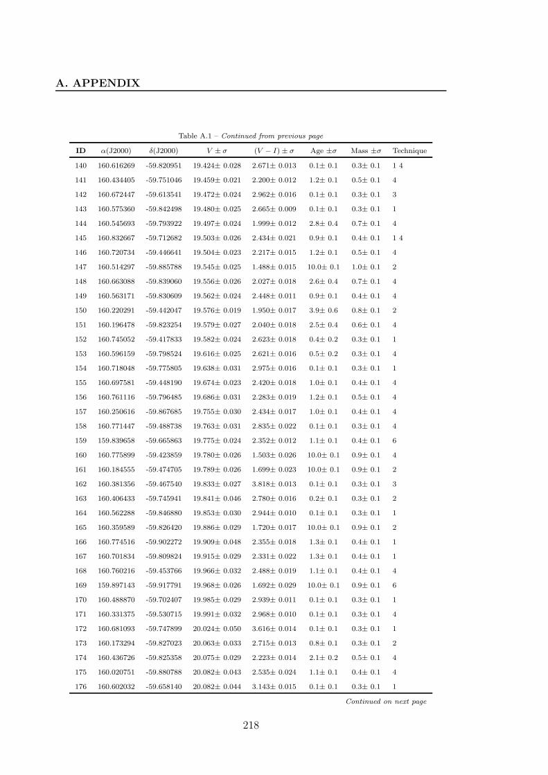
A. APPENDIX
Table A.1 – Continued from previous page
ID α(J2000) δ(J2000) V ± σ (V − I)± σ Age ±σ Mass ±σ Technique
140 160.616269 -59.820951 19.424± 0.028 2.671± 0.013 0.1± 0.1 0.3± 0.1 1 4
141 160.434405 -59.751046 19.459± 0.021 2.200± 0.012 1.2± 0.1 0.5± 0.1 4
142 160.672447 -59.613541 19.472± 0.024 2.962± 0.016 0.1± 0.1 0.3± 0.1 3
143 160.575360 -59.842498 19.480± 0.025 2.665± 0.009 0.1± 0.1 0.3± 0.1 1
144 160.545693 -59.793922 19.497± 0.024 1.999± 0.012 2.8± 0.4 0.7± 0.1 4
145 160.832667 -59.712682 19.503± 0.026 2.434± 0.021 0.9± 0.1 0.4± 0.1 1 4
146 160.720734 -59.446641 19.504± 0.023 2.217± 0.015 1.2± 0.1 0.5± 0.1 4
147 160.514297 -59.885788 19.545± 0.025 1.488± 0.015 10.0± 0.1 1.0± 0.1 2
148 160.663088 -59.839060 19.556± 0.026 2.027± 0.018 2.6± 0.4 0.7± 0.1 4
149 160.563171 -59.830609 19.562± 0.024 2.448± 0.011 0.9± 0.1 0.4± 0.1 4
150 160.220291 -59.442047 19.576± 0.019 1.950± 0.017 3.9± 0.6 0.8± 0.1 2
151 160.196478 -59.823254 19.579± 0.027 2.040± 0.018 2.5± 0.4 0.6± 0.1 4
152 160.745052 -59.417833 19.582± 0.024 2.623± 0.018 0.4± 0.2 0.3± 0.1 1
153 160.596159 -59.798524 19.616± 0.025 2.621± 0.016 0.5± 0.2 0.3± 0.1 4
154 160.718048 -59.775805 19.638± 0.031 2.975± 0.016 0.1± 0.1 0.3± 0.1 1
155 160.697581 -59.448190 19.674± 0.023 2.420± 0.018 1.0± 0.1 0.4± 0.1 4
156 160.761116 -59.796485 19.686± 0.031 2.283± 0.019 1.2± 0.1 0.5± 0.1 4
157 160.250616 -59.867685 19.755± 0.030 2.434± 0.017 1.0± 0.1 0.4± 0.1 4
158 160.771447 -59.488738 19.763± 0.031 2.835± 0.022 0.1± 0.1 0.3± 0.1 4
159 159.839658 -59.665863 19.775± 0.024 2.352± 0.012 1.1± 0.1 0.4± 0.1 6
160 160.775899 -59.423859 19.780± 0.026 1.503± 0.026 10.0± 0.1 0.9± 0.1 4
161 160.184555 -59.474705 19.789± 0.026 1.699± 0.023 10.0± 0.1 0.9± 0.1 2
162 160.381356 -59.467540 19.833± 0.027 3.818± 0.013 0.1± 0.1 0.3± 0.1 3
163 160.406433 -59.745941 19.841± 0.046 2.780± 0.016 0.2± 0.1 0.3± 0.1 2
164 160.562288 -59.846880 19.853± 0.030 2.944± 0.010 0.1± 0.1 0.3± 0.1 1
165 160.359589 -59.826420 19.886± 0.029 1.720± 0.017 10.0± 0.1 0.9± 0.1 2
166 160.774516 -59.902272 19.909± 0.048 2.355± 0.018 1.3± 0.1 0.4± 0.1 1
167 160.701834 -59.809824 19.915± 0.029 2.331± 0.022 1.3± 0.1 0.4± 0.1 1
168 160.760216 -59.453766 19.966± 0.032 2.488± 0.019 1.1± 0.1 0.4± 0.1 4
169 159.897143 -59.917791 19.968± 0.026 1.692± 0.029 10.0± 0.1 0.9± 0.1 6
170 160.488870 -59.702407 19.985± 0.029 2.939± 0.011 0.1± 0.1 0.3± 0.1 1
171 160.331375 -59.530715 19.991± 0.032 2.968± 0.010 0.1± 0.1 0.3± 0.1 4
172 160.681093 -59.747899 20.024± 0.050 3.616± 0.014 0.1± 0.1 0.3± 0.1 1
173 160.173294 -59.827023 20.063± 0.033 2.715± 0.013 0.8± 0.1 0.3± 0.1 2
174 160.436726 -59.825358 20.075± 0.029 2.223± 0.014 2.1± 0.2 0.5± 0.1 4
175 160.020751 -59.880788 20.082± 0.043 2.535± 0.024 1.1± 0.1 0.4± 0.1 4
176 160.602032 -59.658140 20.082± 0.044 3.143± 0.015 0.1± 0.1 0.3± 0.1 1
Continued on next page
218
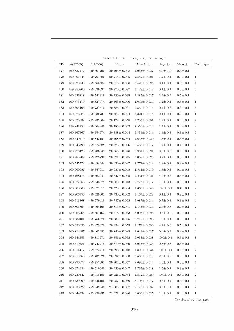
Table A.1 – Continued from previous page
ID α(J2000) δ(J2000) V ± σ (V − I)± σ Age ±σ Mass ±σ Technique
177 160.837272 -59.507790 20.163± 0.048 2.063± 0.027 5.0± 1.0 0.6± 0.1 4
178 160.801848 -59.767580 20.214± 0.035 2.589± 0.021 1.2± 0.1 0.3± 0.1 1
179 160.820948 -59.555584 20.216± 0.036 3.420± 0.025 0.1± 0.1 0.3± 0.1 4
180 159.850860 -59.636697 20.270± 0.027 3.128± 0.012 0.1± 0.1 0.3± 0.1 3
181 160.626818 -59.741319 20.289± 0.035 2.285± 0.027 2.2± 0.2 0.5± 0.1 4
182 160.773279 -59.827574 20.363± 0.040 2.649± 0.024 1.2± 0.1 0.3± 0.1 1
183 159.894496 -59.737510 20.386± 0.031 2.860± 0.014 0.7± 0.3 0.3± 0.1 5
184 160.073586 -59.839734 20.388± 0.034 3.324± 0.014 0.1± 0.1 0.2± 0.1 1
185 160.820832 -59.439064 20.479± 0.055 2.703± 0.031 1.2± 0.1 0.3± 0.1 4
186 159.841354 -59.664940 20.486± 0.042 2.550± 0.014 1.4± 0.1 0.3± 0.1 2
187 160.467667 -59.654774 20.488± 0.044 2.551± 0.014 1.4± 0.1 0.3± 0.1 2
188 160.649510 -59.842151 20.508± 0.034 2.638± 0.020 1.3± 0.1 0.3± 0.1 4
189 160.243190 -59.573888 20.523± 0.036 2.465± 0.017 1.7± 0.1 0.4± 0.1 4
190 160.773423 -59.433648 20.556± 0.046 2.931± 0.021 0.6± 0.3 0.3± 0.1 4
191 160.785809 -59.423738 20.621± 0.045 3.068± 0.025 0.2± 0.1 0.3± 0.1 4
192 160.545773 -59.484644 20.630± 0.037 2.773± 0.013 1.3± 0.1 0.3± 0.1 4
193 160.660687 -59.847911 20.635± 0.048 2.512± 0.019 1.7± 0.1 0.4± 0.1 4
194 160.468475 -59.662941 20.647± 0.045 2.234± 0.021 4.0± 0.6 0.5± 0.1 2
195 160.077556 -59.843072 20.680± 0.043 2.773± 0.017 1.3± 0.1 0.3± 0.1 4
196 160.308868 -59.871311 20.728± 0.084 1.669± 0.048 10.0± 0.1 0.7± 0.1 2
197 160.806156 -59.429061 20.730± 0.062 3.167± 0.028 0.1± 0.1 0.2± 0.1 4
198 160.213868 -59.779419 20.737± 0.052 2.987± 0.014 0.7± 0.3 0.3± 0.1 4
199 160.801895 -59.664165 20.816± 0.051 2.433± 0.034 2.5± 0.3 0.4± 0.1 2
200 159.966965 -59.661163 20.818± 0.053 3.093± 0.026 0.3± 0.2 0.3± 0.1 2
201 160.832401 -59.750670 20.830± 0.055 2.719± 0.023 1.5± 0.1 0.3± 0.1 4
202 160.038696 -59.479828 20.834± 0.053 2.279± 0.030 4.2± 0.6 0.5± 0.1 2
203 160.814697 -59.463681 20.840± 0.088 3.041± 0.027 0.6± 0.4 0.3± 0.1 4
204 160.644553 -59.813771 20.851± 0.052 2.053± 0.028 10.0± 0.1 0.6± 0.1 1
205 160.519581 -59.742278 20.870± 0.059 3.013± 0.035 0.8± 0.3 0.3± 0.1 4
206 160.214417 -59.874210 20.893± 0.048 1.899± 0.034 10.0± 0.1 0.6± 0.1 2
207 160.019358 -59.737023 20.897± 0.063 2.536± 0.019 2.0± 0.2 0.3± 0.1 1
208 160.296672 -59.757082 20.904± 0.057 2.690± 0.014 1.6± 0.1 0.3± 0.1 4
209 160.674684 -59.510640 20.920± 0.047 2.765± 0.018 1.5± 0.1 0.3± 0.1 4
210 160.230347 -59.915180 20.921± 0.054 1.832± 0.029 10.0± 0.1 0.6± 0.1 2
211 160.739090 -59.446106 20.957± 0.059 3.107± 0.017 0.6± 0.4 0.3± 0.1 4
212 160.033722 -59.549648 21.008± 0.057 2.176± 0.037 8.5± 1.4 0.5± 0.1 2
213 160.844292 -59.498935 21.021± 0.096 3.003± 0.025 1.0± 0.4 0.3± 0.1 1
Continued on next page
219
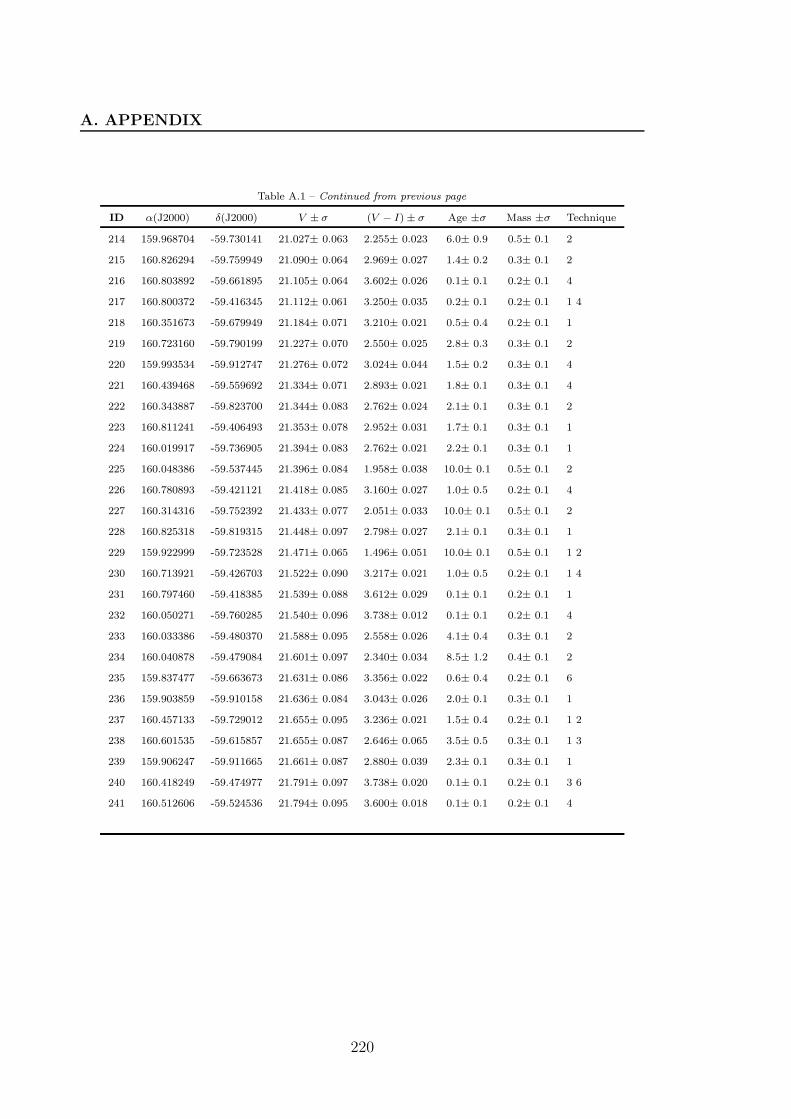
A. APPENDIX
Table A.1 – Continued from previous page
ID α(J2000) δ(J2000) V ± σ (V − I)± σ Age ±σ Mass ±σ Technique
214 159.968704 -59.730141 21.027± 0.063 2.255± 0.023 6.0± 0.9 0.5± 0.1 2
215 160.826294 -59.759949 21.090± 0.064 2.969± 0.027 1.4± 0.2 0.3± 0.1 2
216 160.803892 -59.661895 21.105± 0.064 3.602± 0.026 0.1± 0.1 0.2± 0.1 4
217 160.800372 -59.416345 21.112± 0.061 3.250± 0.035 0.2± 0.1 0.2± 0.1 1 4
218 160.351673 -59.679949 21.184± 0.071 3.210± 0.021 0.5± 0.4 0.2± 0.1 1
219 160.723160 -59.790199 21.227± 0.070 2.550± 0.025 2.8± 0.3 0.3± 0.1 2
220 159.993534 -59.912747 21.276± 0.072 3.024± 0.044 1.5± 0.2 0.3± 0.1 4
221 160.439468 -59.559692 21.334± 0.071 2.893± 0.021 1.8± 0.1 0.3± 0.1 4
222 160.343887 -59.823700 21.344± 0.083 2.762± 0.024 2.1± 0.1 0.3± 0.1 2
223 160.811241 -59.406493 21.353± 0.078 2.952± 0.031 1.7± 0.1 0.3± 0.1 1
224 160.019917 -59.736905 21.394± 0.083 2.762± 0.021 2.2± 0.1 0.3± 0.1 1
225 160.048386 -59.537445 21.396± 0.084 1.958± 0.038 10.0± 0.1 0.5± 0.1 2
226 160.780893 -59.421121 21.418± 0.085 3.160± 0.027 1.0± 0.5 0.2± 0.1 4
227 160.314316 -59.752392 21.433± 0.077 2.051± 0.033 10.0± 0.1 0.5± 0.1 2
228 160.825318 -59.819315 21.448± 0.097 2.798± 0.027 2.1± 0.1 0.3± 0.1 1
229 159.922999 -59.723528 21.471± 0.065 1.496± 0.051 10.0± 0.1 0.5± 0.1 1 2
230 160.713921 -59.426703 21.522± 0.090 3.217± 0.021 1.0± 0.5 0.2± 0.1 1 4
231 160.797460 -59.418385 21.539± 0.088 3.612± 0.029 0.1± 0.1 0.2± 0.1 1
232 160.050271 -59.760285 21.540± 0.096 3.738± 0.012 0.1± 0.1 0.2± 0.1 4
233 160.033386 -59.480370 21.588± 0.095 2.558± 0.026 4.1± 0.4 0.3± 0.1 2
234 160.040878 -59.479084 21.601± 0.097 2.340± 0.034 8.5± 1.2 0.4± 0.1 2
235 159.837477 -59.663673 21.631± 0.086 3.356± 0.022 0.6± 0.4 0.2± 0.1 6
236 159.903859 -59.910158 21.636± 0.084 3.043± 0.026 2.0± 0.1 0.3± 0.1 1
237 160.457133 -59.729012 21.655± 0.095 3.236± 0.021 1.5± 0.4 0.2± 0.1 1 2
238 160.601535 -59.615857 21.655± 0.087 2.646± 0.065 3.5± 0.5 0.3± 0.1 1 3
239 159.906247 -59.911665 21.661± 0.087 2.880± 0.039 2.3± 0.1 0.3± 0.1 1
240 160.418249 -59.474977 21.791± 0.097 3.738± 0.020 0.1± 0.1 0.2± 0.1 3 6
241 160.512606 -59.524536 21.794± 0.095 3.600± 0.018 0.1± 0.1 0.2± 0.1 4
220
References
Abbott D. C., 1982, ApJ, 263, 723 3
Abbott D. C., Conti P. S., 1987, ARA&A, 25, 113 39
Adelman-McCarthy J. K., Agueros M. A., Allam S. S., et al., 2006, ApJS, 162, 38 xxxii, 109
Akerlof C., Amrose S., Balsano R., et al., 2000, AJ, 119, 1901 23
Alard C., 2000, A&AS, 144, 363 194
Alard C., Lupton R. H., 1998, ApJ, 503, 325 194
Aldering G., Humphreys R. M., Richmond M., 1994, AJ, 107, 662 84, 152
Allen L. E., Myers P. C., Di Francesco J., Mathieu R., Chen H., Young E., 2002, ApJ, 566, 993 76
Anderson J. P., Covarrubias R. A., James P. A., Hamuy M., Habergham S. M., 2010, MNRAS,
407, 2660 108
Anderson J. P., James P. A., 2009, MNRAS, 399, 559 83
Arcavi I., Gal-Yam A., Kasliwal e. a. M. M., et al., 2010, ApJ, 721, 777 9, 23, 108, 109
Arcavi I., Gal-Yam A., Yaron O., et al., 2011, ApJ, 742, L18 17, 84, 92
Arnett D., 1995, ARA&A, 33, 115 3, 39
Arnett D., 1996, Supernovae and nucleosynthesis: an investigation of the history of matter, from
the Big Bang to the present, Princeton University Press. 3, 39
Arnett W. D., 1980, ApJ, 237, 541 98
Arnett W. D., 1982, ApJ, 253, 785 98
Arnett W. D., Bahcall J. N., Kirshner R. P., Woosley S. E., 1989, ARA&A, 27, 629 152
Arnett W. D., Fu A., 1989, ApJ, 340, 396 98, 100, 102, 110
Ascenso J., Alves J., Vicente S., Lago M. T. V. T., 2007, A&A, 476, 199 74
Atwood W. B., Abdo A. A., Ackermann M., et al., 2009, ApJ, 697, 1071 23
221
REFERENCES
Ballesteros-Paredes J., Klessen R. S., Mac Low M.-M., Vazquez-Semadeni E., 2007, Protostars
and Planets V, 63–80 76
Barbon R., Benetti S., Cappellaro E., Patat F., Turatto M., Iijima T., 1995, A&AS, 110, 513 xxxi,
17, 92, 93, 106
Barentsen G., Vink J. S., Drew J. E., et al., 2011, MNRAS, 415, 103 67, 68
Barkat Z., Rakavy G., Sack N., 1967, Physical Review Letters, 18, 379 17
Baron E., Nugent P. E., Branch D., Hauschildt P. H., 2004, ApJ, 616, L91 184
Baron E., Nugent P. E., Branch D., Hauschildt P. H., 2005, in 1604-2004: Supernovae as Cos-
mological Lighthouses, edited by M. Turatto, S. Benetti, L. Zampieri, W. Shea, vol. 342 of
Astronomical Society of the Pacific Conference Series, 351 102
Barrett P., 1988, MNRAS, 234, 937 114, 130
Barthelmy S. D., Barbier L. M., Cummings J. R., et al., 2005, Space Sci. Rev., 120, 143 23
Bayless A. J., Pritchard T. A., Roming P. W. A., et al., 2013, ApJ, 764, L13 116
Bazin G., Palanque-Delabrouille N., Rich J., et al., 2009, A&A, 499, 653 xxxvii, 189, 190
Beauchemin M., 1985, M.Sc. Thesis, Laval University 26
Becker W., Fenkart R., 1971, A&AS, 4, 241 48
Benetti S., 2000, Mem. Soc. Astron. Italiana, 71, 323 16
Benetti S., Cappellaro E., Turatto M., Pastorello A., 2000, IAU Circ., 7375, 2 83
Benson P. J., Herbst W., Salzer J. J., et al., 1994, AJ, 107, 1453 17
Bergemann M., Kudritzki R.-P., Plez B., Davies B., Lind K., Gazak Z., 2012, ApJ, 751, 156 5
Bergemann M., Kudritzki R.-P., Wurl M., Plez B., Davies B., Gazak Z., 2013, ApJ, 764, 115 5
Bersten M. C., Benvenuto O., Hamuy M., 2011, ApJ, 729, 61 192
Bersten M. C., Benvenuto O. G., Folatelli G., et al., 2014, AJ, 148, 68 153
Bersten M. C., Benvenuto O. G., Nomoto K., et al., 2012, ApJ, 757, 31 84, 91, 99, 101, 102, 192
Bersten M. C., Hamuy M., 2009, ApJ, 701, 200 xl, 104, 105, 111
Bersten M. C., Tanaka M., Tominaga N., Benvenuto O. G., Nomoto K., 2013, ApJ, 767, 143 192
Bertout C., 1989, ARA&A, 27, 351 53
Bertout C., Basri G., Bouvier J., 1988, ApJ, 330, 350 64
Bessell M. S., Brett J. M., 1988, PASP, 100, 1134 xxviii, 58
Bester M., Danchi W. C., Hale D., et al., 1996, ApJ, 463, 336 12
222
REFERENCES
Bethe H. A., Wilson J. R., 1985, ApJ, 295, 14 19
Beuther H., Linz H., Henning T., eds., 2008, Massive Star Formation: Observations Confront
Theory, vol. 387 of Astronomical Society of the Pacific Conference Series 10
Bietenholz M. F., Brunthaler A., Soderberg A. M., et al., 2012, ApJ, 751, 125 84
Bionta R. M., Blewitt G., Bratton C. B., Casper D., Ciocio A., 1987, Physical Review Letters, 58,
1494 130
Bisnovatyi-Kogan G. S., Kazhdan Y. M., 1967, SvA, 10, 604 17
Blaauw A., 1964, ARA&A, 2, 213 10, 11
Blaauw A., 1991, in NATO ASIC Proc. 342: The Physics of Star Formation and Early Stellar
Evolution, edited by C. J. Lada, N. D. Kylafis, 125 11
Blanc G., Afonso C., Alard C., et al., 2004, A&A, 423, 881 xxxvii, 181, 189, 190
Blinnikov S. I., Eastman R., Bartunov O. S., Popolitov V. A., Woosley S. E., 1998, ApJ, 496, 454
91
Blondin S., Modjaz M., Kirshner R., Challis P., Berlind P., 2006, Central Bureau Electronic
Telegrams, 757, 1 131
Blondin S., Tonry J. L., 2007, ApJ, 666, 1024 85, 92, 192, 198
Bloom J. S., Richards J. W., Nugent P. E., et al., 2012, PASP, 124, 1175 195
Boiani J., Rice S. A., 1969, Physical Review, 185, 931 166
Borra E. F., 1982, JRASC, 76, 245 26, 27, 30, 142, 151
Borra E. F., 1993, A&A, 278, 665 142
Borra E. F., 1994, ArXiv Astrophysics e-prints 144, 172
Borra E. F., 2001a, ArXiv Astrophysics e-prints 186, 190
Borra E. F., 2001b, ArXiv Astrophysics e-prints 182, 186, 191
Borra E. F., 2003, A&A, 404, 47 182, 186, 191
Borra E. F., Beauchemin M., Arsenault R., Lalande R., 1985, PASP, 97, 454 26
Borra E. F., Content R., Boily E., 1988, PASP, 100, 1399 27
Borra E. F., Content R., Drinkwater M. J., Szapiel S., 1989, ApJ, 346, L41 141
Borra E. F., Content R., Girard L., Szapiel S., Tremblay L. M., Boily E., 1992, ApJ, 393, 829 141,
144
Borra E. F., Tremblay G., Huot Y., Gauvin J., 1997, PASP, 109, 319 166
223
REFERENCES
Bose S., Kumar B., Sutaria F., et al., 2013, MNRAS, 433, 1871 xxxiii, 115, 117, 123, 126, 128, 140
Botticella M. T., Riello M., Cappellaro E., et al., 2008, A&A, 479, 49 xxxvii, 189, 190, 194
Bouwman J., Lawson W. A., Dominik C., et al., 2006, ApJ, 653, L57 68
Branch D., Baron E., Jeffery D. J., 2001, ArXiv Astrophysics e-prints, arXiv:astro-ph/0111573
102
Branch D., Benetti S., Kasen D., et al., 2002, ApJ, 566, 1005 83, 102, 107
Branch D., Miller D. L., 1993, ApJ, 405, L5 183
Branch D., Nomoto K., Filippenko A. V., 1991, Comments on Astrophysics, 15, 221 181
Branch D., Tammann G. A., 1992, ARA&A, 30, 359 183
Briceno C., Preibisch T., Sherry W. H., et al., 2007, Protostars and Planets V, 345–360 10, 59
Brink H., Richards J. W., Poznanski D., et al., 2013, MNRAS, 435, 1047 195
Brooks K. J., Cox P., Schneider N., et al., 2003, A&A, 412, 751 74
Brooks K. J., Storey J. W. V., Whiteoak J. B., 2001, MNRAS, 327, 46 41
Broos P. S., Townsley L. K., Feigelson E. D., Getman K. V., Bauer F. E., Garmire G. P., 2010,
ApJ, 714, 1582 63
Bruenn S. W., Mezzacappa A., Hix W. R., et al., 2009, Journal of Physics Conference Series, 180,
1, 012018 9
Bruenn S. W., Mezzacappa A., Hix W. R., et al., 2013, ApJ, 767, L6 9
Burrows A., 2000, Nature, 403, 727 xxv, 19
Burrows A., 2013, Reviews of Modern Physics, 85, 245 9, 21
Burrows A., Hayes J., Fryxell B. A., 1995, ApJ, 450, 830 19
Cabanac R. A., 1997, ArXiv Astrophysics e-prints 32
Cabanac R. A., Borra E. F., Beauchemin M., 1998, ApJ, 509, 309 xxvi, 32
Cao Y., Kasliwal M. M., Arcavi I., et al., 2013, ApJ, 775, L7 153
Cappellaro E., Evans R., Turatto M., 1999, A&A, 351, 459 183, 190
Cappellaro E., Riello M., Altavilla G., et al., 2005, A&A, 430, 83 192, 194
Cappellaro E., Turatto M., Tsvetkov D. Y., et al., 1997, A&A, 322, 431 23
Carraro G., Patat F., 2001, A&A, 379, 136 41, 48
Carraro G., Patat F., Baumgardt H., 2001, A&A, 371, 107 41
Carraro G., Romaniello M., Ventura P., Patat F., 2004, A&A, 418, 525 41, 48, 50
224
REFERENCES
Cartwright A., Whitworth A. P., 2004, MNRAS, 348, 589 76
Castor J. I., Abbott D. C., Klein R. I., 1975, ApJ, 195, 157 10
Chabrier G., 2003, PASP, 115, 763 69
Chatzopoulos E., Wheeler J. C., Vinko J., 2009, ApJ, 704, 1251 98
Chatzopoulos E., Wheeler J. C., Vinko J., 2012, ApJ, 746, 121 102
Chauhan N., Pandey A. K., Ogura K., et al., 2009, MNRAS, 396, 964 67
Chauhan N., Pandey A. K., Ogura K., et al., 2011, MNRAS, 415, 1202 67
Chevalier R. A., 1992, ApJ, 394, 599 92
Chevalier R. A., Fransson C., 2008, ApJ, 683, L135 92
Chevalier R. A., Soderberg A. M., 2010, ApJ, 711, L40 17, 84
Chini R., Kruegel E., 1983, A&A, 117, 289 49
Chini R., Wargau W. F., 1990, A&A, 227, 213 48, 49
Chiosi C., Maeder A., 1986, ARA&A, 24, 329 5, 6, 8
Chornock R., Filippenko A. V., Li W., et al., 2011, ApJ, 739, 41 84
Chornock R., Filippenko A. V., Li W., Silverman J. M., 2010, ApJ, 713, 1363 114, 130, 132
Chugai N. N., 1991, MNRAS, 250, 513 16
Chugai N. N., 1992, Soviet Astronomy Letters, 18, 168 113
Chugai N. N., 2006, Astronomy Letters, 32, 739 22, 114
Ciabattari F., Mazzoni E., Jin Z., et al., 2011, Central Bureau Electronic Telegrams, 2827, 1 85,
92
Claeskens J.-F., Gosset E., Naze Y., Rauw G., Vreux J.-M., 2011, A&A, 525, A142 xxxix, 41, 45,
51, 52, 60, 61, 62, 80
Claria J. J., 1977, A&AS, 27, 145 48
Clayton G. C., Wolff M. J., Gordon K. D., Smith P. S., Nordsieck K. H., Babler B. L., 2004, AJ,
127, 3382 125
Clocchiatti A., Wheeler J. C., Phillips M. M., et al., 1997, ApJ, 483, 675 84
Cohen J. G., Persson S. E., Elias J. H., Frogel J. A., 1981, ApJ, 249, 481 xxviii, 58, 59, 64
Conley A., Sullivan M., Hsiao E. Y., et al., 2008, ApJ, 681, 482 196
Conti P. S., 1984, in Observational Tests of the Stellar Evolution Theory, edited by A. Maeder,
A. Renzini, vol. 105 of IAU Symposium, 233 6
225
REFERENCES
Conti P. S., Massey P., 1989, ApJ, 337, 251 7
Conti P. S., Niemela V. S., Walborn N. R., 1979, ApJ, 228, 206 42
Contini T., Treyer M. A., Sullivan M., Ellis R. S., 2002, MNRAS, 330, 75 108
Corbelli E., Palla F., Zinnecker H., eds., 2005, The Initial Mass Function 50 years later, vol. 327
of Astrophysics and Space Science Library 69
Covino S., Stefanon M., Sciuto G., et al., 2004, in Ground-based Instrumentation for Astronomy,
edited by A. F. M. Moorwood, M. Iye, vol. 5492 of Society of Photo-Optical Instrumentation
Engineers (SPIE) Conference Series, 1613–1622 23
Cox P., 1995, in The Eta Carinae Region: A Laboratory of Stellar Evolution, eds. V. Niemela, N.
Morrell, & A. Feinstein, Rev. Mexicana Astron. Astrofis. Ser. Conf., 2, 105 41
Crockett R. M., Eldridge J. J., Smartt S. J., et al., 2008, MNRAS, 391, L5 84, 153
Cropper M., Bailey J., McCowage J., Cannon R. D., Couch W. J., 1988, MNRAS, 231, 695 114,
130
Crowther P. A., 2007, ARA&A, 45, 177 6, 7, 40, 153
Crowther P. A., Hillier D. J., Smith L. J., 1995, A&A, 293, 403 42
Cucciati O., Tresse L., Ilbert O., et al., 2012, A&A, 539, A31 181
Cutispoto G., Zerbi F. M., Chincarini G., REM/Ross Team, 2004, Baltic Astronomy, 13, 307 23
Cutri R. M., Skrutskie M. F., van Dyk S., et al., 2003, VizieR Online Data Catalog, 2246, 0 45
Dahlen T., Goobar A., 2002, PASP, 114, 284 192, 196
Dahlen T., Strolger L.-G., Riess A. G., 2008, ApJ, 681, 462 xxxvii, 181, 189, 190
Dahlen T., Strolger L.-G., Riess A. G., et al., 2004, ApJ, 613, 189 xxxvii, 189, 190
Davies B., Kudritzki R.-P., Figer D. F., 2010, MNRAS, 407, 1203 5
de Graauw T., Lidholm S., Fitton B., et al., 1981, A&A, 102, 257 41
Deep A., Fiorentino G., Tolstoy E., et al., 2011, A&A, 531, A151 186
DeGioia-Eastwood K., Throop H., Walker G., Cudworth K. M., 2001, ApJ, 549, 578 43, 48
Denis S., 2011, Test report - angular velocity stability of ILMT primary mirror with mercury
(3mm). Tech. Rep., AMOS 142
Dessart L., Hillier D. J., 2005a, A&A, 439, 671 184
Dessart L., Hillier D. J., 2005b, A&A, 437, 667 xl, 104, 105, 111
Dessart L., Hillier D. J., 2011, MNRAS, 410, 1739 113
226
REFERENCES
Dessart L., Hillier D. J., Waldman R., Livne E., Blondin S., 2012, MNRAS, 426, L76 18
Dickel H. R., 1974, A&A, 31, 11 41
Dilday B., Kessler R., Frieman J. A., et al., 2008, ApJ, 682, 262 xxxvii, 189, 190
Dilday B., Smith M., Bassett B., et al., 2010, ApJ, 713, 1026 189
Doi T., Nakano S., Itagaki K., Naito H., Iizuka R., 2007, Central Bureau Electronic Telegrams,
848, 1 132
Drake A. J., Djorgovski S. G., Mahabal A., et al., 2009, ApJ, 696, 870 23
Drissen L., Moffat A. F. J., Walborn N. R., Shara M. M., 1995, AJ, 110, 2235 10
Drout M. R., Massey P., Meynet G., 2012, ApJ, 750, 97 6
Drout M. R., Soderberg A. M., Gal-Yam A., et al., 2011, ApJ, 741, 97 92, 94, 96
Dufour R. J., van Orsow D., Walter D. K., Hester J. J., Currie D. G., 1998, in Astrophysical
plasmas - near and far, eds. R. J. Dufour, & S. Torres-Peimbert, Rev. Mexicana Astron. Astrofis.
Ser. Conf., 7, 217 41
Ekstrom S., Georgy C., Eggenberger P., et al., 2012, A&A, 537, A146 5
Eldridge J. J., Fraser M., Smartt S. J., Maund J. R., Crockett R. M., 2013, MNRAS, 436, 774
xxvi, 9, 24, 25
Elias-Rosa N., Van Dyk S. D., Li W., et al., 2009, ApJ, 706, 1174 152
Elias-Rosa N., Van Dyk S. D., Li W., et al., 2010, ApJ, 714, L254 153
Elmegreen B. G., 1998, in Origins, edited by C. E. Woodward, J. M. Shull, H. A. Thronson, Jr.,
vol. 148 of Astronomical Society of the Pacific Conference Series, 150 10, 39
Elmhamdi A., Danziger I. J., Branch D., Leibundgut B., Baron E., Kirshner R. P., 2006, A&A,
450, 305 83, 102
Elmhamdi A., Danziger I. J., Chugai N., et al., 2003, MNRAS, 338, 939 130
Ergon M., Sollerman J., Fraser M., et al., 2014, A&A, 562, A17 98
Espinoza P., Selman F. J., Melnick J., 2009, A&A, 501, 563 69
Eswaraiah C., Maheswar G., Pandey A. K., Jose J., Ramaprakash A. N., Bhatt H. C., 2013, A&A,
556, A65 120
Eswaraiah C., Pandey A. K., Maheswar G., et al., 2011, MNRAS, 411, 1418 120
Eswaraiah C., Pandey A. K., Maheswar G., Chen W. P., Ojha D. K., Chandola H. C., 2012,
MNRAS, 419, 2587 120
227
REFERENCES
Fagotti P., Dimai A., Quadri U., et al., 2012, Central Bureau Electronic Telegrams, 3054, 1 115
Falck B. L., Riess A. G., Hlozek R., 2010, ApJ, 723, 398 196
Falk S. W., Arnett W. D., 1977, ApJS, 33, 515 84, 128
Feigelson E. D., Broos P., Gaffney III J. A., et al., 2002, ApJ, 574, 258 63
Feigelson E. D., Montmerle T., 1999, ARA&A, 37, 363 11, 52
Feinstein A., 1981, PASP, 93, 202 48
Feinstein A., 1983, Ap&SS, 96, 293 48
Feinstein A., 1995, in The Eta Carinae Region: A Laboratory of Stellar Evolution, eds. V. Niemela,
N. Morrell, & A. Feinstein, Rev. Mexicana Astron. Astrofis. Ser. Conf., 2, 57 39
Feinstein A., Marraco H. G., Muzzio J. C., 1973, A&AS, 12, 331 47, 48
Fesen R. A., 2001, ApJS, 133, 161 21
Filippenko A. V., 1988, AJ, 96, 1941 83, 84
Filippenko A. V., 1991, in Supernovae and Stellar Evolution, edited by A. Ray, T. Velusamy, 58
13, 15
Filippenko A. V., 1997, ARA&A, 35, 309 13, 83, 197
Filippenko A. V., Chornock R., 2003, IAU Circ., 8084, 4 83
Filippenko A. V., Leonard D. C., 2004, in Cosmic explosions in three dimensions, edited by
P. Hoflich, P. Kumar, J. C. Wheeler, 30 21, 114
Filippenko A. V., Li W. D., Treffers R. R., Modjaz M., 2001, in IAU Colloq. 183: Small Telescope
Astronomy on Global Scales, edited by B. Paczynski, W.-P. Chen, C. Lemme, vol. 246 of
Astronomical Society of the Pacific Conference Series, 121 182, 189
Finet F., 2013, in PhD Thesis, University of Liege, Belgium, 13–170 xxvi, xl, 27, 28, 144, 145,
151, 168, 172, 173, 187
Fisher A., Branch D., Nugent P., Baron E., 1997, ApJ, 481, L89 102
Fitzgerald M. P., Mehta S., 1987, MNRAS, 228, 545 48
Folatelli G., Gonzalez S., Morrell N., 2007, Central Bureau Electronic Telegrams, 850, 1 132
Forte J. C., 1978, AJ, 83, 1199 47
Fowler W. A., Hoyle F., 1964, ApJS, 9, 201 3, 17
Fraley G. S., 1967, Supernovae Explosions Induced by Pair Production Instability., Ph.D. thesis,
CALIFORNIA INSTITUTE OF TECHNOLOGY. 17
228
REFERENCES
Fraser M., Maund J. R., Smartt S. J., et al., 2012, ApJ, 759, L13 115, 116
Fraser M., Takats K., Pastorello A., et al., 2010, ApJ, 714, L280 153
Freedman W. L., Madore B. F., Gibson B. K., et al., 2001, ApJ, 553, 47 115
Fremling C., Sollerman J., Taddia F., et al., 2014, A&A, 565, A114 153
Freyer T., Hensler G., Yorke H. W., 2003, ApJ, 594, 888 10
Fryer C. L., 1999, ApJ, 522, 413 21, 83
Gaczkowski B., Preibisch T., Ratzka T., Roccatagliata V., Ohlendorf H., Zinnecker H., 2013, A&A,
549, A67 42, 54, 58, 64, 72, 74
Gal-Yam A., 2012, Science, 337, 927 17
Gal-Yam A., Kasliwal M. M., Arcavi I., et al., 2011, ApJ, 736, 159 84
Gal-Yam A., Leonard D. C., 2009, Nature, 458, 865 9, 16
Gal-Yam A., Leonard D. C., Fox D. B., et al., 2007, ApJ, 656, 372 16
Gal-Yam A., Mazzali P., Ofek E. O., et al., 2009, Nature, 462, 624 17, 18
Garay G., Lizano S., 1999, PASP, 111, 1049 39
Garmire G. P., Bautz M. W., Ford P. G., Nousek J. A., Ricker Jr. G. R., 2003, in Society of Photo-
Optical Instrumentation Engineers (SPIE) Conf. Ser., eds. J. E. Truemper & H. D. Tananbaum,
vol. 4851, 28–44 62
Garnett D. R., 2002, ApJ, 581, 1019 109
Getman K. V., Flaccomio E., Broos P. S., et al., 2005, ApJS, 160, 319 63
Ghosh S. K., Iyengar K. V. K., Rengarajan T. N., Tandon S. N., Verma R. P., Daniel R. R., 1988,
ApJ, 330, 928 41
Giavalisco M., Ferguson H. C., Koekemoer A. M., et al., 2004, ApJ, 600, L93 189
Gibson B. K., 1991, JRASC, 85, 158 25, 26
Gibson B. K., Hickson P., 1991, in The Space Distribution of Quasars, edited by D. Crampton,
vol. 21 of Astronomical Society of the Pacific Conference Series, 80–83 31
Gibson B. K., Hickson P., 1992, MNRAS, 258, 543 147
Glassgold A. E., Huggins P. J., 1986, ApJ, 306, 605 12
Gomez M., Hartmann L., Kenyon S. J., Hewett R., 1993, AJ, 105, 1927 76
Gong Y., Cooray A., Chen X., 2010, ApJ, 709, 1420 196
Gorosabel J., de Ugarte Postigo A., Castro-Tirado A. J., et al., 2010, A&A, 522, A14 132, 133
229
REFERENCES
Gorosabel J., Larionov V., Castro-Tirado A. J., et al., 2006, A&A, 459, L33 23, 113
Gosset E., Naze Y., Sana H., Rauw G., Vreux J.-M., 2009, A&A, 508, 805 42, 48, 60
Gosset E., Remy M., Manfroid J., et al., 1991, Information Bulletin on Variable Stars, 3571, 1 42
Grabelsky D. A., Cohen R. S., Bronfman L., Thaddeus P., 1988, ApJ, 331, 181 39
Grassberg E. K., Imshennik V. S., Nadyozhin D. K., 1971, Ap&SS, 10, 28 128
Graur O., Poznanski D., Maoz D., et al., 2011, MNRAS, 417, 916 181, 189
Graur O., Rodney S. A., Maoz D., et al., 2014, ApJ, 783, 28 181, 189
Green D. A., Stephenson F. R., 2003, in Supernovae and Gamma-Ray Bursters, edited by
K. Weiler, vol. 598 of Lecture Notes in Physics, Berlin Springer Verlag, 7–19 12
Gritschneder M., Burkert A., Naab T., Walch S., 2010, ApJ, 723, 971 10, 72
Groh J. H., Georgy C., Ekstrom S., 2013a, A&A, 558, L1 153
Groh J. H., Meynet G., Georgy C., Ekstrom S., 2013b, A&A, 558, A131 8, 25
Guetter H. H., Vrba F. J., 1989, AJ, 98, 611 47
Gunther H. M., Wolk S. J., Spitzbart B., et al., 2012, AJ, 144, 101 78
Gutermuth R. A., Megeath S. T., Myers P. C., Allen L. E., Pipher J. L., Fazio G. G., 2009, ApJS,
184, 18 55, 76, 78
Gutermuth R. A., Megeath S. T., Pipher J. L., et al., 2005, ApJ, 632, 397 55, 76
Gutermuth R. A., Myers P. C., Megeath S. T., et al., 2008, ApJ, 674, 336 76
Guy J., Astier P., Baumont S., et al., 2007, A&A, 466, 11 196
Guy J., Astier P., Nobili S., Regnault N., Pain R., 2005, A&A, 443, 781 196
Hadfield L. J., Crowther P. A., Schild H., Schmutz W., 2005, A&A, 439, 265 8
Hadfield L. J., van Dyk S. D., Morris P. W., Smith J. D., Marston A. P., Peterson D. E., 2007,
MNRAS, 376, 248 153
Hadjiyska E., Rabinowitz D., Baltay C., et al., 2011, The Astronomer’s Telegram, 3812, 1 23
Hamaguchi K., Petre R., Matsumoto H., et al., 2007, PASJ, 59, 151 41
Hamann W.-R., Duennebeil G., Koesterke L., Wessolowski U., Schmutz W., 1991, A&A, 249, 443
42
Hamuy M., Deng J., Mazzali P. A., et al., 2009, ApJ, 703, 1612 xxxi, 84, 96, 106
Hamuy M., Walker A. R., Suntzeff N. B., Gigoux P., Heathcote S. R., Phillips M. M., 1992, PASP,
104, 533 45
230
REFERENCES
Han J., 2009, in IAU Symposium, edited by K. G. Strassmeier, A. G. Kosovichev, J. E. Beckman,
vol. 259 of IAU Symposium, 455–466 125
Hardin D., Afonso C., Alard C., et al., 2000, A&A, 362, 419 xxxvii, 189, 190
Harper G. M., Brown A., 2006, ApJ, 646, 1179 12
Harper G. M., Brown A., Guinan E. F., 2008, AJ, 135, 1430 12
Harper G. M., Brown A., Lim J., 2001, ApJ, 551, 1073 12
Harutyunyan A. H., Pfahler P., Pastorello A., et al., 2008, A&A, 488, 383 198
Harvey P. M., Hoffmann W. F., Campbell M. F., 1979, ApJ, 227, 114 41
Hatano K., Branch D., Fisher A., Millard J., Baron E., 1999, ApJS, 121, 233 107
Heger A., Fryer C. L., Woosley S. E., Langer N., Hartmann D. H., 2003a, ApJ, 591, 288 xxv, 20,
83
Heger A., Fryer C. L., Woosley S. E., Langer N., Hartmann D. H., 2003b, ApJ, 591, 288 21, 153
Heger A., Woosley S. E., 2002, ApJ, 567, 532 17
Heger A., Woosley S. E., 2010, ApJ, 724, 341 18
Heiles C., 1996, in Polarimetry of the Interstellar Medium, edited by W. G. Roberge, D. C. B.
Whittet, vol. 97 of Astronomical Society of the Pacific Conference Series, 457 125
Heiles C., 2000, AJ, 119, 923 xxxii, 117, 121
Herbig G. H., Bell K. R., 1988, Third Catalog of Emission-Line Stars of the Orion Population : 3
: 1988 53
Herbst W., 1976, ApJ, 208, 923 47
Hickson P., 2008a, Analysis and recommendations concerning the ILMT primary mirror, air bear-
ing, interface and air system, Tech. Rep. R01, The University of British Columbia 142, 143,
158
Hickson P., 2008b, Requirements for the ILMT primary mirror system, Tech. Rep. R02, The
University of British Columbia 143
Hickson P., Borra E. F., Cabanac R., et al., 1998, in Advanced Technology Optical/IR Telescopes
VI, edited by L. M. Stepp, vol. 3352 of Society of Photo-Optical Instrumentation Engineers
(SPIE) Conference Series, 226–232 34
Hickson P., Borra E. F., Cabanac R., Content R., Gibson B. K., Walker G. A. H., 1994, ApJ, 436,
L201 xxvi, 31, 32
Hickson P., Gibson B. K., Hogg D. W., 1993, PASP, 105, 501 144
231
REFERENCES
Hickson P., Mulrooney M. K., 1998, ApJS, 115, 35 32
Hickson P., Pfrommer T., Cabanac R., et al., 2007, PASP, 119, 444 27, 34, 137, 174
Hickson P., Racine R., 2007, PASP, 119, 456 34
Hickson P., Richardson E. H., 1998, PASP, 110, 1081 138, 147, 151
Hillenbrand L. A., 1997, AJ, 113, 1733 10
Hillenbrand L. A., 2005, arXiv:astro-ph/0511083 67
Hillenbrand L. A., Bauermeister A., White R. J., 2008, in 14th Cambridge Workshop on Cool
Stars, Stellar Systems, and the Sun, edited by G. van Belle, ASP Conf. Ser., 384, 200 67
Hillenbrand L. A., Hartmann L. W., 1998, ApJ, 492, 540 10
Hillenbrand L. A., Strom S. E., Vrba F. J., Keene J., 1992, ApJ, 397, 613 59
Hillier D. J., Davidson K., Ishibashi K., Gull T., 2001, ApJ, 553, 837 41
Hirata K., Kajita T., Koshiba M., Nakahata M., Oyama Y., 1987, Physical Review Letters, 58,
1490 130
Hodapp K. W., Kaiser N., Aussel H., et al., 2004, Astronomische Nachrichten, 325, 636 23
Hoeflich P., 1995, ApJ, 440, 821 22, 114
Hoflich P., 1991, A&A, 246, 481 113, 114
Hoflich P., Khokhlov A., Wang L., 2001, in 20th Texas Symposium on relativistic astrophysics,
edited by J. C. Wheeler, H. Martel, vol. 586 of American Institute of Physics Conference Series,
459–471 113
Hopkins A. M., 2004, ApJ, 615, 209 181
Hopkins A. M., Beacom J. F., 2006, ApJ, 651, 142 181
Horesh A., Poznanski D., Ofek E. O., Maoz D., 2008, MNRAS, 389, 1871 xxxvii, 189, 190
Horesh A., Stockdale C., Fox D. B., et al., 2013, MNRAS, 436, 1258 84
Horne K., 1986, PASP, 98, 609 88
Hough J. H., Bailey J. A., Rouse M. F., Whittet D. C. B., 1987, MNRAS, 227, 1P 124
Houk N., Cowley A. P., 1975, University of Michigan Catalogue of two-dimensional spectral types
for the HD stars. Volume I 51
Howell S. B., 1989, PASP, 101, 616 186
Howell S. B., 2000, Handbook of CCD Astronomy 147, 186
Hoyle F., Fowler W. A., 1960, ApJ, 132, 565 3, 19
232
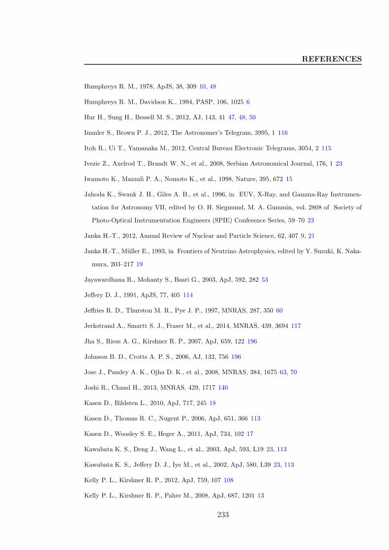
REFERENCES
Humphreys R. M., 1978, ApJS, 38, 309 10, 48
Humphreys R. M., Davidson K., 1994, PASP, 106, 1025 6
Hur H., Sung H., Bessell M. S., 2012, AJ, 143, 41 47, 48, 50
Immler S., Brown P. J., 2012, The Astronomer’s Telegram, 3995, 1 116
Itoh R., Ui T., Yamanaka M., 2012, Central Bureau Electronic Telegrams, 3054, 2 115
Ivezic Z., Axelrod T., Brandt W. N., et al., 2008, Serbian Astronomical Journal, 176, 1 23
Iwamoto K., Mazzali P. A., Nomoto K., et al., 1998, Nature, 395, 672 15
Jahoda K., Swank J. H., Giles A. B., et al., 1996, in EUV, X-Ray, and Gamma-Ray Instrumen-
tation for Astronomy VII, edited by O. H. Siegmund, M. A. Gummin, vol. 2808 of Society of
Photo-Optical Instrumentation Engineers (SPIE) Conference Series, 59–70 23
Janka H.-T., 2012, Annual Review of Nuclear and Particle Science, 62, 407 9, 21
Janka H.-T., Muller E., 1993, in Frontiers of Neutrino Astrophysics, edited by Y. Suzuki, K. Naka-
mura, 203–217 19
Jayawardhana R., Mohanty S., Basri G., 2003, ApJ, 592, 282 53
Jeffery D. J., 1991, ApJS, 77, 405 114
Jeffries R. D., Thurston M. R., Pye J. P., 1997, MNRAS, 287, 350 60
Jerkstrand A., Smartt S. J., Fraser M., et al., 2014, MNRAS, 439, 3694 117
Jha S., Riess A. G., Kirshner R. P., 2007, ApJ, 659, 122 196
Johnson B. D., Crotts A. P. S., 2006, AJ, 132, 756 196
Jose J., Pandey A. K., Ojha D. K., et al., 2008, MNRAS, 384, 1675 63, 70
Joshi R., Chand H., 2013, MNRAS, 429, 1717 140
Kasen D., Bildsten L., 2010, ApJ, 717, 245 18
Kasen D., Thomas R. C., Nugent P., 2006, ApJ, 651, 366 113
Kasen D., Woosley S. E., Heger A., 2011, ApJ, 734, 102 17
Kawabata K. S., Deng J., Wang L., et al., 2003, ApJ, 593, L19 23, 113
Kawabata K. S., Jeffery D. J., Iye M., et al., 2002, ApJ, 580, L39 23, 113
Kelly P. L., Kirshner R. P., 2012, ApJ, 759, 107 108
Kelly P. L., Kirshner R. P., Pahre M., 2008, ApJ, 687, 1201 13
233
REFERENCES
Khokhlov A., Hoflich P., 2001, in Explosive Phenomena in Astrophysical Compact Objects, edited
by H.-Y. Chang, C.-H. Lee, M. Rho, I. Yi, vol. 556 of American Institute of Physics Conference
Series, 301–312 113
Kim A. G., Miquel R., 2007, Astroparticle Physics, 28, 448 192
Kingsburgh R. L., Barlow M. J., Storey P. J., 1995, A&A, 295, 75 7
Kippenhahn R., Weigert A., 1990, Stellar Structure and Evolution 17
Kirshner R. P., 1990, in Supernovae, edited by A. G. Petschek, 59–75 13
Kirshner R. P., Kwan J., 1974, ApJ, 193, 27 184
Kleiser I. K. W., Poznanski D., Kasen D., et al., 2011, MNRAS, 415, 372 152
Kobulnicky H. A., Zaritsky D., 1999, ApJ, 511, 118 108
Kochanek C. S., Khan R., Dai X., 2012, ApJ, 759, 20 116
Kolmogorov A., 1941, Akademiia Nauk SSSR Doklady, 30, 301 3
Kotak R., Meikle P., Pozzo M., et al., 2006, ApJ, 651, L117 130
Kotake K., Sumiyoshi K., Yamada S., et al., 2012, Progress of Theoretical and Experimental
Physics, 2012, 1, 010000 9
Kozyreva A., Yoon S.-C., Langer N., 2014, A&A, 566, A146 17
Krause O., Birkmann S. M., Usuda T., et al., 2008, Science, 320, 1195 12
Krauss M. I., Soderberg A. M., Chomiuk L., et al., 2012, ApJ, 750, L40 84
Kroupa P., 2002, Science, 295, 82 69
Kudritzki R.-P., Puls J., 2000, ARA&A, 38, 613 10
Kumar B., Pandey S. B., Eswaraiah C., Gorosabel J., 2014a, MNRAS, 442, 2 vii, x
Kumar B., Pandey S. B., Sahu D. K., et al., 2013, MNRAS, 431, 308 vii, ix, xxxix, 17, 100, 140
Kumar B., Sagar R., Rautela B. S., Srivastava J. B., Srivastava R. K., 2000, Bulletin of the
Astronomical Society of India, 28, 675 87
Kumar B., Sharma S., Manfroid J., et al., 2014b, A&A, 567, A109 vii, ix, xxvii, 40
Kunz M., Bassett B. A., Hlozek R. A., 2007, Phys. Rev. D, 75, 10, 103508 192, 196
Kuroda T., Kotake K., Takiwaki T., 2012, ApJ, 755, 11 9
Kuznetsova N., Barbary K., Connolly B., et al., 2008, ApJ, 673, 981 xxxvii, 189, 190
Kuznetsova N. V., Connolly B. M., 2007, ApJ, 659, 530 196
Lada C. J., Alves J., Lada E. A., 1996, AJ, 111, 1964 76
234
REFERENCES
Lada C. J., Lada E. A., 2003, ARA&A, 41, 57 10, 70
Lancon A., Gallagher J. S., Mouhcine M., Smith L. J., Ladjal D., de Grijs R., 2009, Ap&SS, 324,
241 5
Landolt A. U., 2009, AJ, 137, 4186 87
Le Floc’h E., Papovich C., Dole H., et al., 2005, ApJ, 632, 169 181
Leaman J. F., Li W., Filippenko A., LOSS, 2009, in American Astronomical Society Meeting
Abstracts 214, vol. 214 of American Astronomical Society Meeting Abstracts, 316.02 23
Leibundgut B., Suntzeff N. B., 2003, in Supernovae and Gamma-Ray Bursters, edited by K.Weiler,
vol. 598 of Lecture Notes in Physics, Berlin Springer Verlag, 77–90 195
Leinert C., Bowyer S., Haikala L. K., et al., 1998, A&AS, 127, 1 xxxiv, 142
Leitherer C., Robert C., Drissen L., 1992, ApJ, 401, 596 3
Leloudas G., Gallazzi A., Sollerman J., et al., 2011, A&A, 530, A95 108
Lennarz D., Altmann D., Wiebusch C., 2012, A&A, 538, A120 xxvi, 15, 24
Leonard D. C., 2007, ArXiv e-prints xxvi, 22
Leonard D. C., Dessart L., Hillier D. J., Pignata G., 2012a, in American Institute of Physics
Conference Series, edited by J. L. Hoffman, J. Bjorkman, B. Whitney, vol. 1429 of American
Institute of Physics Conference Series, 204–207 114, 130, 132
Leonard D. C., Filippenko A. V., 2001, PASP, 113, 920 23, 113, 114
Leonard D. C., Filippenko A. V., 2005, in 1604-2004: Supernovae as Cosmological Lighthouses,
edited by M. Turatto, S. Benetti, L. Zampieri, W. Shea, vol. 342 of Astronomical Society of
the Pacific Conference Series, 330 113, 114
Leonard D. C., Filippenko A. V., Ardila D. R., Brotherton M. S., 2001, ApJ, 553, 861 113, 114,
125, 130
Leonard D. C., Filippenko A. V., Chornock R., Li W., 2002, AJ, 124, 2506 125
Leonard D. C., Filippenko A. V., Ganeshalingam M., et al., 2006, Nature, 440, 505 114, 130
Leonard D. C., Pignata G., Dessart L., et al., 2012b, The Astronomer’s Telegram, 4033, 1 117
Levato H., Malaroda S., 1981, PASP, 93, 714 48
Levato H., Malaroda S., 1982, PASP, 94, 807 48
Lewis J. R., Walton N. A., Meikle W. P. S., et al., 1994, MNRAS, 266, L27 xxxi, 84, 90, 92, 93,
94, 96, 98, 99, 106
235
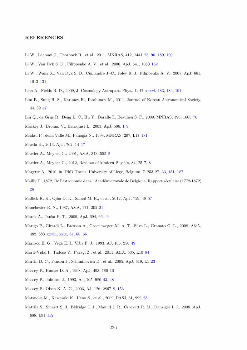
REFERENCES
Li W., Leaman J., Chornock R., et al., 2011, MNRAS, 412, 1441 23, 96, 189, 190
Li W., Van Dyk S. D., Filippenko A. V., et al., 2006, ApJ, 641, 1060 152
Li W., Wang X., Van Dyk S. D., Cuillandre J.-C., Foley R. J., Filippenko A. V., 2007, ApJ, 661,
1013 131
Lien A., Fields B. D., 2009, J. Cosmology Astropart. Phys., 1, 47 xxxvi, 183, 184, 191
Lim B., Sung H. S., Karimov R., Ibrahimov M., 2011, Journal of Korean Astronomical Society,
44, 39 47
Liu Q., de Grijs R., Deng L. C., Hu Y., Baraffe I., Beaulieu S. F., 2009, MNRAS, 396, 1665 70
Mackey J., Bromm V., Hernquist L., 2003, ApJ, 586, 1 9
Madau P., della Valle M., Panagia N., 1998, MNRAS, 297, L17 181
Maeda K., 2013, ApJ, 762, 14 17
Maeder A., Meynet G., 2001, A&A, 373, 555 8
Maeder A., Meynet G., 2012, Reviews of Modern Physics, 84, 25 7, 8
Magette A., 2010, in PhD Thesis, University of Liege, Belgium, 7–253 27, 33, 151, 187
Mailly E., 1872, De l’astronomie dans l’Academie royale de Belgique. Rapport seculaire (1772-1872)
26
Mallick K. K., Ojha D. K., Samal M. R., et al., 2012, ApJ, 759, 48 57
Manchester R. N., 1987, A&A, 171, 205 21
Marek A., Janka H.-T., 2009, ApJ, 694, 664 9
Marigo P., Girardi L., Bressan A., Groenewegen M. A. T., Silva L., Granato G. L., 2008, A&A,
482, 883 xxviii, xxix, 64, 65, 66
Marraco H. G., Vega E. I., Vrba F. J., 1993, AJ, 105, 258 49
Martı-Vidal I., Tudose V., Paragi Z., et al., 2011, A&A, 535, L10 84
Martin D. C., Fanson J., Schiminovich D., et al., 2005, ApJ, 619, L1 23
Massey P., Hunter D. A., 1998, ApJ, 493, 180 10
Massey P., Johnson J., 1993, AJ, 105, 980 43, 48
Massey P., Olsen K. A. G., 2003, AJ, 126, 2867 8, 153
Matsuoka M., Kawasaki K., Ueno S., et al., 2009, PASJ, 61, 999 23
Mattila S., Smartt S. J., Eldridge J. J., Maund J. R., Crockett R. M., Danziger I. J., 2008, ApJ,
688, L91 152
236
REFERENCES
Maund J. R., Fraser M., Ergon M., et al., 2011, ApJ, 739, L37 84, 153
Maund J. R., Smartt S. J., 2005, MNRAS, 360, 288 152
Maund J. R., Smartt S. J., Danziger I. J., 2005, MNRAS, 364, L33 152
Maund J. R., Smartt S. J., Kudritzki R. P., Podsiadlowski P., Gilmore G. F., 2004, Nature, 427,
129 84, 152
Maund J. R., Spyromilio J., Hoflich P. A., et al., 2013, MNRAS, 433, L20 23, 113
Maund J. R., Wheeler J. C., Patat F., Wang L., Baade D., Hoflich P. A., 2007, ApJ, 671, 1944
23, 113, 125
Maurer I., Mazzali P. A., Taubenberger S., Hachinger S., 2010, MNRAS, 409, 1441 83
Mauron N., Josselin E., 2011, A&A, 526, A156 5
Mayya Y. D., 1991, Journal of Astrophysics and Astronomy, 12, 319 185
Mazzali P. A., Deng J., Hamuy M., Nomoto K., 2009, ApJ, 703, 1624 84
Mazzali P. A., Deng J., Maeda K., et al., 2002, ApJ, 572, L61 15
Mazzali P. A., Deng J., Tominaga N., et al., 2003, ApJ, 599, L95 15
Mazzali P. A., Iwamoto K., Nomoto K., 2000, ApJ, 545, 407 15
McCall M. L., 1984, MNRAS, 210, 829 114
McLean I. S., 1989, Electronic and computer-aided astronomy: From eyes to electronic sensors
185
Medhi B. J., Maheswar G., Pandey J. C., Tamura M., Sagar R., 2010, MNRAS, 403, 1577 119
Melbourne J., Salzer J. J., 2002, AJ, 123, 2302 108
Melinder J., 2011, in PhD Thesis, Stockholm University, Sweden, 1–71 197
Mendez M., Clocchiatti A., Benvenuto O. G., Feinstein C., Marraco H. G., 1988, ApJ, 334, 295
114
Meyer M. R., Calvet N., Hillenbrand L. A., 1997, AJ, 114, 288 xxviii, 58
Meynet G., Maeder A., Schaller G., Schaerer D., Charbonnel C., 1994, A&AS, 103, 97 9
Milisavljevic D., Margutti R., Soderberg A. M., et al., 2013, ApJ, 767, 71 84, 92, 96
Miller G. E., Scalo J. M., 1978, PASP, 90, 506 70
Miller G. E., Scalo J. M., 1979, ApJS, 41, 513 69
Minkowski R., 1941, PASP, 53, 224 13
237
REFERENCES
Modjaz M., Kewley L., Bloom J. S., Filippenko A. V., Perley D., Silverman J. M., 2011, ApJ, 731,
L4 108
Moffat A. F. J., Drissen L., Shara M. M., 1994, ApJ, 436, 183 10
Monard L. A. G., 2007, Central Bureau Electronic Telegrams, 845, 1 83
Morrell N., Garcia B., Levato H., 1988, PASP, 100, 1431 48
Morrell N., Stritzinger M., 2008, Central Bureau Electronic Telegrams, 1335, 1 132
Moskvitin A. S., Sonbas E., Sokolov V. V., Fatkhullin T. A., Castro-Tirado A. J., 2010, Astro-
physical Bulletin, 65, 132 107
Motte F., Andre P., Neri R., 1998, A&A, 336, 150 76
Muench A. A., Lada E. A., Lada C. J., 2000, ApJ, 533, 358 70
Muller E., 1994, in Supernovae, edited by S. A. Bludman, R. Mochkovitch, J. Zinn-Justin, 393 19
Mulrooney M., 2000, A 3.0 meter liquid mirror telescope, Ph.D. thesis, RICE UNIVERSITY 172
Munari U., Henden A., Belligoli R., et al., 2013, New A, 20, 30 116
Munari U., Vagnozzi A., Castellani F., 2012, Central Bureau Electronic Telegrams, 3054, 3 115
Munari U., Zwitter T., 1997, A&A, 318, 269 94
Nakano S., Itagaki K., Kadota K., 2006, Central Bureau Electronic Telegrams, 756, 1 131
Nakar E., Sari R., 2010, ApJ, 725, 904 92, 192
Neill J. D., Sullivan M., Balam D., et al., 2006, AJ, 132, 1126 xxxvii, 189, 190
Niemela V. S., 1979, in Mass Loss and Evolution of O-Type Stars, edited by P. S. Conti, C. W. H.
De Loore, vol. 83 of IAU Symposium, 291–293 42
Ninane N. M., Jamar C. A., 1996, Appl. Opt., 35, 6131 33
Nomoto K., Maeda K., Umeda H., Ohkubo T., Deng J., Mazzali P., 2003, in A Massive Star
Odyssey: From Main Sequence to Supernova, eds. K. van der Hucht, A. Herrero, & C. Esteban,
vol. 212 of IAU Symposium, 395 39
Nugent P., Kim A., Perlmutter S., 2002, PASP, 114, 803 196
Oates S. R., Bayless A. J., Stritzinger M. D., et al., 2012, MNRAS, 424, 1297 84, 96
Oguri M., Marshall P. J., 2010, MNRAS, 405, 2579 xxxvii, 190
Ojha D. K., Tamura M., Nakajima Y., et al., 2004, ApJ, 608, 797 59
Okada Y., Onaka T., Shibai H., Doi Y., 2003, A&A, 412, 199 49
Okumura J. E., Ihara Y., Doi M., et al., 2014, PASJ, 66, 49 181, 189
238
REFERENCES
Olsson-Steel D., 1986, JRASC, 80, 128 25
Pain R., Fabbro S., Sullivan M., et al., 2002, ApJ, 577, 120 xxxvii, 189, 190
Pain R., Hook I. M., Deustua S., et al., 1996, ApJ, 473, 356 191
Paliya V. S., Stalin C. S., Kumar B., et al., 2013, MNRAS, 428, 2450 140
Pandey A. K., Ogura K., Sekiguchi K., 2000, PASJ, 52, 847 48
Pandey A. K., Sharma S., Ogura K., et al., 2008, MNRAS, 383, 1241 63, 70
Pandey A. K., Upadhyay K., Nakada Y., Ogura K., 2003, A&A, 397, 191 48, 49
Pandey J. C., Medhi B. J., Sagar R., Pandey A. K., 2009, MNRAS, 396, 1004 120
Papaliolios C., Krasovska M., Koechlin L., Nisenson P., Standley C., 1989, Nature, 338, 565 21
Paris I., Petitjean P., Aubourg E., et al., 2014, A&A, 563, A54 195
Parker J. W., Garmany C. D., 1993, AJ, 106, 1471 10
Pastorello A., Kasliwal M. M., Crockett R. M., et al., 2008, MNRAS, 389, 955 xxxi, 84, 92, 95,
96, 98, 99, 106
Patat F., Barbon R., Cappellaro E., Turatto M., 1993, A&AS, 98, 443 16
Patat F., Barbon R., Cappellaro E., Turatto M., 1994, A&A, 282, 731 16
Patat F., Carraro G., 2001, MNRAS, 325, 1591 48
Patat F., Hoflich P., Baade D., Maund J. R., Wang L., Wheeler J. C., 2012, A&A, 545, A7 23,
113
Paturel G., Petit C., Prugniel P., et al., 2003, A&A, 412, 45 115
Pauldrach A., Puls J., Kudritzki R. P., 1986, A&A, 164, 86 10
Pauldrach A., Puls J., Kudritzki R. P., Mendez R. H., Heap S. R., 1988, A&A, 207, 123 9
Pereyra A., Magalhaes A. M., Rodrigues C. V., et al., 2006, A&A, 454, 827 130
Perrett K., Sullivan M., Conley A., et al., 2012, AJ, 144, 59 181, 189
Pfrommer T., Hickson P., She C.-Y., Vance J. D., 2008, in Society of Photo-Optical Instrumenta-
tion Engineers (SPIE) Conference Series, vol. 7015 of Society of Photo-Optical Instrumentation
Engineers (SPIE) Conference Series 34
Pires A. M., Motch C., Turolla R., Treves A., Popov S. B., 2009, A&A, 498, 233 41
Podsiadlowski P., Joss P. C., Hsu J. J. L., 1992, ApJ, 391, 246 84
Poels J., Borra E., Hickson P., et al., 2012, in IAU Symposium, edited by E. Griffin, R. Hanisch,
R. Seaman, vol. 285 of IAU Symposium, 394–396 182
239
REFERENCES
Potter A. E., Mulrooney M., 1997, Advances in Space Research, 19, 213 32
Povich M. S., Smith N., Majewski S. R., et al., 2011, ApJS, 194, 14 39, 42, 50, 54, 57, 58, 72, 75
Poznanski D., Gal-Yam A., Maoz D., Filippenko A. V., Leonard D. C., Matheson T., 2002, PASP,
114, 833 196
Poznanski D., Maoz D., Gal-Yam A., 2007a, AJ, 134, 1285 196
Poznanski D., Maoz D., Yasuda N., et al., 2007b, MNRAS, 382, 1169 xxxvii, 189, 190, 194
Poznanski D., Prochaska J. X., Bloom J. S., 2012, MNRAS, 426, 1465 123
Preibisch T., 2011, in Reviews in Modern Astronomy: Zooming in: The Cosmos at High Reso-
lution, Volume 23 (ed R. von Berlepsch), Wiley-VCH Verlag GmbH & Co. KGaA, Weinheim,
Germany. doi: 10.1002/9783527644384.ch13 11
Preibisch T., Hodgkin S., Irwin M., et al., 2011a, ApJS, 194, 10 11, 49
Preibisch T., Ratzka T., Gehring T., et al., 2011b, A&A, 530, A40 55
Preibisch T., Ratzka T., Kuderna B., et al., 2011c, A&A, 530, A34 10, 11, 42, 59, 60, 70
Preibisch T., Schuller F., Ohlendorf H., Pekruhl S., Menten K. M., Zinnecker H., 2011d, A&A,
525, A92 11, 42
Preibisch T., Zinnecker H., 2007, in IAU Symposium, edited by B. G. Elmegreen, J. Palous, vol.
237 of IAU Symposium, 270–277 10
Prieto J., 2009, Central Bureau Electronic Telegrams, 2087, 1 84
Prieto J. L., Stanek K. Z., Beacom J. F., 2008, ApJ, 673, 999 xxxii, 108, 109
Prisinzano L., Micela G., Flaccomio E., et al., 2008, ApJ, 677, 401 52
Pritchet C. J., Howell D. A., Sullivan M., 2008, ApJ, 683, L25 181
Puls J., Vink J. S., Najarro F., 2008, A&A Rev., 16, 209 84
Qiu Y., Li W., Qiao Q., Hu J., 1999, AJ, 117, 736 84, 93, 94, 96
Quimby R. M., Kulkarni S. R., Kasliwal M. M., et al., 2011, Nature, 474, 487 17
Quimby R. M., Wheeler J. C., Hoflich P., Akerlof C. W., Brown P. J., Rykoff E. S., 2007, ApJ,
666, 1093 106, 108
Quimby R. M., Yuan F., Akerlof C., Wheeler J. C., 2013, MNRAS, 431, 912 17
Rakavy G., Shaviv G., 1967, ApJ, 148, 803 17
Ramaprakash A. N., Gupta R., Sen A. K., Tandon S. N., 1998, A&AS, 128, 369 119
Rana N. C., 1991, ARA&A, 29, 129 69
240
REFERENCES
Rathborne J. M., Burton M. G., Brooks K. J., Cohen M., Ashley M. C. B., Storey J. W. V., 2002,
MNRAS, 331, 85 41, 74
Rau A., Kulkarni S. R., Law N. M., et al., 2009, PASP, 121, 1334 23
Rautela B. S., Joshi G. C., Pandey J. C., 2004, Bulletin of the Astronomical Society of India, 32,
159 xxxii, 118, 119, 120
Rauw G., Manfroid J., De Becker M., 2010, A&A, 511, A25 53
Rauw G., Vreux J.-M., Gosset E., Hutsemekers D., Magain P., Rochowicz K., 1996, A&A, 306,
771 42
Remillard R. A., McClintock J. E., 2006, ARA&A, 44, 49 3
Richardson D., Branch D., Baron E., 2006, AJ, 131, 2233 92
Richardson D., Branch D., Casebeer D., Millard J., Thomas R. C., Baron E., 2002, AJ, 123, 745
96, 184
Richer M. G., McCall M. L., 1995, ApJ, 445, 642 108
Richmond M. W., Treffers R. R., Filippenko A. V., et al., 1994, AJ, 107, 1022 17, 84
Riess A. G., Nugent P. E., Gilliland R. L., et al., 2001, ApJ, 560, 49 196
Riess A. G., Press W. H., Kirshner R. P., 1995, ApJ, 438, L17 196
Riess A. G., Press W. H., Kirshner R. P., 1996, ApJ, 473, 88 196
Robin A. C., Reyle C., Derriere S., Picaud S., 2003, A&A, 409, 523 70
Robitaille T. P., Meade M. R., Babler B. L., et al., 2008, AJ, 136, 2413 57
Robitaille T. P., Whitney B. A., Indebetouw R., Wood K., Denzmore P., 2006, ApJS, 167, 256 59
Roccatagliata V., Preibisch T., Ratzka T., Gaczkowski B., 2013, A&A, 554, A6 11, 42, 49, 72, 73
Rodney S. A., Riess A. G., Strolger L.-G., et al., 2014, AJ, 148, 13 189
Rodney S. A., Tonry J. L., 2009, ApJ, 707, 1064 196
Rodney S. A., Tonry J. L., 2010, ApJ, 723, 47 189
Roming P., Prieto J., Milne P. A., 2009a, Central Bureau Electronic Telegrams, 2093, 1 84
Roming P., Pritchard T., Brown P., et al., 2010, in American Astronomical Society Meeting
Abstracts #215, vol. 42 of Bulletin of the American Astronomical Society, 342.03 93
Roming P. W. A., Pritchard T. A., Brown P. J., et al., 2009b, ApJ, 704, L118 84, 92
Rujopakarn W., Eisenstein D. J., Rieke G. H., et al., 2010, ApJ, 718, 1171 181
Russell D. G., 2002, ApJ, 565, 681 115
241
REFERENCES
Ryder S. D., Murrowood C. E., Stathakis R. A., 2006, MNRAS, 369, L32 84
Sagar R., Kumar B., Omar A., 2013, ArXiv e-prints 140, 198
Sagar R., Kumar B., Omar A., Joshi Y. C., 2012, in Astronomical Society of India Conference
Series, vol. 4 of Astronomical Society of India Conference Series, 173 87, 139, 140, 198
Sagar R., Omar A., Kumar B., et al., 2011, Current Science, 101, 8 87, 139
Saha A., Sandage A., Tammann G. A., Labhardt L., Macchetto F. D., Panagia N., 1999, ApJ,
522, 802 183
Salpeter E. E., 1955, ApJ, 121, 161 3, 69, 70, 81
Salpeter E. E., 1964, ApJ, 140, 796 192
Sanders N. E., Soderberg A. M., Foley R. J., et al., 2013, ApJ, 769, 39 13
Sanders N. E., Soderberg A. M., Levesque E. M., et al., 2012, ApJ, 758, 132 108, 109
Scalo J., 1998, in The Stellar Initial Mass Function (38th Herstmonceux Conference), eds. G.
Gilmore, & D. Howell, ASP Conf. Ser., 142, 201 69
Scalo J. M., 1986, Fund. Cosmic Phys., 11, 1 69
Scarrott S. M., Rolph C. D., Semple D. P., 1990, in Galactic and Intergalactic Magnetic Fields,
edited by R. Beck, R. Wielebinski, P. P. Kronberg, vol. 140 of IAU Symposium, 245–251 125
Scarrott S. M., Rolph C. D., Wolstencroft R. W., Tadhunter C. N., 1991, MNRAS, 249, 16P 125
Schiminovich D., Ilbert O., Arnouts S., et al., 2005, ApJ, 619, L47 181
Schlegel D. J., Finkbeiner D. P., Davis M., 1998, ApJ, 500, 525 94, 123
Schmidt B., 2012, in IAU Symposium, edited by E. Griffin, R. Hanisch, R. Seaman, vol. 285 of
IAU Symposium, 9–10 192
Schmidt B. P., Kirshner R. P., Eastman R. G., et al., 1993, Nature, 364, 600 84
Schmidt G. D., Elston R., Lupie O. L., 1992, AJ, 104, 1563 120
Schmidt-Kaler T., 1982, in Landolt-Bornstein: Numerical Data and Functional Relationship in
Science and Technology, Vol. 2b. eds. K. Schaifers, H. H. Voigt, H. Landolt (Springer-Verlag),
Berlin, p. 19 xxvii, 45, 46
Schnurr O., Moffat A. F. J., St-Louis N., Morrell N. I., Guerrero M. A., 2008, MNRAS, 389, 806 8
Schroeder D. J., 1987, Astronomical optics 151
Serkowski K., 1970, ApJ, 160, 1083 21
Serkowski K., Mathewson D. S., Ford V. L., 1975, ApJ, 196, 261 123, 125
242
REFERENCES
Shapiro P. R., Sutherland P. G., 1982, ApJ, 263, 902 21, 114
Shara M. M., Moffat A. F. J., Smith L. F., Niemela V. S., Potter M., Lamontagne R., 1999, AJ,
118, 390 153
Sharma S., Pandey A. K., Ojha D. K., et al., 2007, MNRAS, 380, 1141 70
Sharma S., Pandey A. K., Pandey J. C., et al., 2012, PASJ, 64, 107 63
Shields G. A., 1978, Nature, 272, 706 192
Shigeyama T., Suzuki T., Kumagai S., Nomoto K., Saio H., Yamaoka H., 1994, ApJ, 420, 341 91
Siess L., Dufour E., Forestini M., 2000, A&A, 358, 593 xxviii, xxix, 64, 65, 66, 67, 70
Siviero A., Tomasella L., Pastorello A., et al., 2012, Central Bureau Electronic Telegrams, 3054, 4
115
Skillman E. D., Kennicutt R. C., Hodge P. W., 1989, ApJ, 347, 875 108
Smartt S. J., 2009, ARA&A, 47, 63 83, 152
Smartt S. J., Eldridge J. J., Crockett R. M., Maund J. R., 2009, MNRAS, 395, 1409 9, 23, 152
Smartt S. J., Maund J. R., Hendry M. A., et al., 2004, Science, 303, 499 152
Smith N., 2002, MNRAS, 331, 7 47
Smith N., 2006a, MNRAS, 367, 763 11, 39, 40, 74
Smith N., 2006b, ApJ, 644, 1151 50
Smith N., 2010, in Hot and Cool: Bridging Gaps in Massive Star Evolution, edited by C. Leitherer,
P. D. Bennett, P. W. Morris, J. T. Van Loon, vol. 425 of Astronomical Society of the Pacific
Conference Series, 63 xxv, 7, 16
Smith N., Bally J., Morse J. A., 2003, ApJ, 587, L105 41
Smith N., Brooks K. J., 2007, MNRAS, 379, 1279 11
Smith N., Brooks K. J., 2008, The Carina Nebula: A Laboratory for Feedback and Triggered Star
Formation, 138 11, 39, 40, 41, 42, 46, 50, 74
Smith N., Chornock R., Li W., et al., 2008a, ApJ, 686, 467 9
Smith N., Egan M. P., Carey S., Price S. D., Morse J. A., Price P. A., 2000, ApJ, 532, L145 xxvii,
40, 41
Smith N., Foley R. J., Bloom J. S., et al., 2008b, ApJ, 686, 485 9
Smith N., Hinkle K. H., Ryde N., 2009, AJ, 137, 3558 12, 16
Smith N., Li W., Filippenko A. V., Chornock R., 2011, MNRAS, 412, 1522 xxvi, 9, 24, 25
243
REFERENCES
Smith N., McCray R., 2007, ApJ, 671, L17 9
Smith N., Povich M. S., Whitney B. A., et al., 2010, MNRAS, 406, 952 11, 42, 64, 74, 78, 80
Smith R. G., 1987, MNRAS, 227, 943 47
Soderberg A. M., Chevalier R. A., Kulkarni S. R., Frail D. A., 2006, ApJ, 651, 1005 83
Soderberg A. M., Margutti R., Zauderer B. A., et al., 2012, ApJ, 752, 78 84
Sonbas E., Moskvitin A. S., Fatkhullin T. A., et al., 2008, Astrophysical Bulletin, 63, 228 84, 104
Stalin C. S., Gopal Krishna, Sagar R., Wiita P. J., 2004, Journal of Astrophysics and Astronomy,
25, 1 192
Stassun K. G., Ardila D. R., Barsony M., Basri G., Mathieu R. D., 2004, AJ, 127, 3537 52
Stetson P. B., 1987, PASP, 99, 191 43, 87, 175
Stetson P. B., 1992, in Astronomical Data Analysis Software and Systems I, eds. D. M. Worrall,
C. Biemesderfer, & J. Barnes, ASP Conf. Ser., 25, 297 43, 87, 175
Stockdale C. J., Ryder S. D., Van Dyk S. D., et al., 2012, The Astronomer’s Telegram, 4012, 1
116
Stoll R., Prieto J. L., Stanek K. Z., Pogge R. W., 2013, ApJ, 773, 12 108
Stritzinger M., 2010, Central Bureau Electronic Telegrams, 2158, 1 84
Stritzinger M., Mazzali P., Phillips M. M., et al., 2009, ApJ, 696, 713 83
Sullivan M., Howell D. A., Perrett K., et al., 2006, AJ, 131, 960 196
Sung H., Bessell M. S., Lee S.-W., 1997, AJ, 114, 2644 xxvii, 53, 54
Surdej J., Absil O., Bartczak P., et al., 2006, in Society of Photo-Optical Instrumentation Engi-
neers (SPIE) Conference Series, vol. 6267 of Society of Photo-Optical Instrumentation Engineers
(SPIE) Conference Series 151, 182, 183, 187
Taddia F., Sollerman J., Leloudas G., et al., 2014, ArXiv e-prints 192
Taddia F., Stritzinger M. D., Sollerman J., et al., 2013, A&A, 555, A10 16
Tammann G. A., Leibundgut B., 1990, A&A, 236, 9 183
Tammann G. A., Sandage A., 1995, ApJ, 452, 16 183
Tanaka M., Kawabata K. S., Hattori T., et al., 2012, ApJ, 754, 63 23, 113
Tapia M., Roth M., Marraco H., Ruiz M. T., 1988, MNRAS, 232, 661 47, 48
Tapia M., Roth M., Vazquez R. A., Feinstein A., 2003, MNRAS, 339, 44 43, 48, 50
Taubenberger S., Navasardyan H., Maurer J. I., et al., 2011, MNRAS, 413, 2140 84
244
REFERENCES
Taylor M., Cinabro Y., Dilday B., et al., 2014, The Astrophysical Journal, 792, 2, 135 187, 190
Teixeira P. S., Lada C. J., Young E. T., et al., 2006, ApJ, 636, L45 76
Telleschi A., Gudel M., Briggs K. R., Audard M., Palla F., 2007, A&A, 468, 425 52
The P. S., Bakker R., Tjin A Djie H. R. E., 1980, A&A, 89, 209 47, 48
The P. S., Vleeming G., 1971, A&A, 14, 120 48
Tomasella L., Valenti S., Ochner P., Benetti S., Cappellaro E., Pastorello A., 2011, Central Bureau
Electronic Telegrams, 2827, 2 86
Tonry J., Davis M., 1979, AJ, 84, 1511 197
Townsley L. K., Broos P. S., Corcoran M. F., et al., 2011, ApJS, 194, 1 42, 54, 62, 63
Tremonti C. A., Heckman T. M., Kauffmann G., et al., 2004, ApJ, 613, 898 108
Turatto M., 2003, in Supernovae and Gamma-Ray Bursters, edited by K. Weiler, vol. 598 of
Lecture Notes in Physics, Berlin Springer Verlag, 21–36 xxv, 13, 15
Turner D. G., Grieve G. R., Herbst W., Harris W. E., 1980, AJ, 85, 1193 48
Ugliano M., Janka H.-T., Marek A., Arcones A., 2012, ApJ, 757, 69 21
Umeda H., Nomoto K., 2002, ApJ, 565, 385 17
Umeda H., Nomoto K., 2008, ApJ, 673, 1014 18
Utrobin V. P., 2007, A&A, 461, 233 128
van der Hucht K. A., 2001, New A Rev., 45, 135 8
van der Hucht K. A., 2006, A&A, 458, 453 153
van der Hucht K. A., Conti P. S., Lundstrom I., Stenholm B., 1981, Space Sci. Rev., 28, 227 42
Van Dyk S. D., Cenko S. B., Poznanski D., et al., 2012, ApJ, 756, 131 116, 152
Van Dyk S. D., Davidge T. J., Elias-Rosa N., et al., 2010, ArXiv e-prints 132
Van Dyk S. D., Li W., Cenko S. B., et al., 2011, ApJ, 741, L28 84
Van Dyk S. D., Li W., Filippenko A. V., 2003a, PASP, 115, 1 152
Van Dyk S. D., Li W., Filippenko A. V., 2003b, PASP, 115, 1289 152
van Genderen A. M., 2001, A&A, 366, 508 6
van Leeuwen F., 2007, A&A, 474, 653 xxxii, xl, 12, 117, 121
Vanbeveren D., De Loore C., Van Rensbergen W., 1998, A&A Rev., 9, 63 8
Vangeyte B., Manfroid J., Surdej J., 2002, A&A, 388, 712 138, 147
Vazquez R. A., Baume G., Feinstein A., Prado P., 1996, A&AS, 116, 75 43, 47, 48, 50
245
REFERENCES
Veron-Cetty M.-P., Veron P., 2010, A&A, 518, A10 195
Vink J. S., 2008, in IAU Symposium, edited by L. Deng, K. L. Chan, vol. 252 of IAU Symposium,
271–281 10
Vink J. S., 2012, in Astrophysics and Space Science Library, edited by K. Davidson, R. M.
Humphreys, vol. 384 of Astrophysics and Space Science Library, 221 6
Vinko J., Takats K., Szalai T., et al., 2012, A&A, 540, A93 84, 95, 96
Walborn N. R., 1973, ApJ, 179, 517 48
Walborn N. R., 1982, AJ, 87, 1300 48
Wang J., Townsley L. K., Feigelson E. D., et al., 2007, ApJS, 168, 100 63
Wang L., Baade D., Hoflich P., et al., 2003a, ApJ, 591, 1110 23, 113, 124, 129
Wang L., Baade D., Hoflich P., Wheeler J. C., 2003b, ApJ, 592, 457 129
Wang L., Howell D. A., Hoflich P., Wheeler J. C., 2001, ApJ, 550, 1030 113
Wang L., Wheeler J. C., 1996, ApJ, 462, L27 114
Wang L., Wheeler J. C., 2008, ARA&A, 46, 433 22
Wang Y., 2007, ApJ, 654, L123 192
Ward-Thompson D., Andre P., Crutcher R., Johnstone D., Onishi T., Wilson C., 2007, Protostars
and Planets V, eds. B. Reipurth, D. Jewitt, & K. Keil, 33–46 76
Waxman E., Meszaros P., Campana S., 2007, ApJ, 667, 351 92
Wheeler J. C., 2000, in American Institute of Physics Conference Series, edited by S. S. Holt,
W. W. Zhang, vol. 522 of American Institute of Physics Conference Series, 445–466 113
Wheeler J. C., Barker E., Benjamin R., et al., 1993, ApJ, 417, L71 92, 93
Wheeler J. C., Filippenko A. V., 1996, in IAU Colloq. 145: Supernovae and Supernova Remnants,
edited by T. S. Kuhn, 241 114
Wheeler J. C., Harkness R. P., 1990, Reports on Progress in Physics, 53, 1467 xxv, 14
White R. J., Basri G., 2003, ApJ, 582, 1109 53
Whittet D. C. B., ed., 2003, Dust in the galactic environment 47
Widenhorn R., Blouke M. M., Weber A., Rest A., Bodegom E., 2002, in Sensors and Camera
Systems for Scientific, Industrial, and Digital Photography Applications III, edited by M. M.
Blouke, J. Canosa, N. Sampat, vol. 4669 of Society of Photo-Optical Instrumentation Engineers
(SPIE) Conference Series, 193–201 146
246
Williams J. P., Blitz L., McKee C. F., 2000, Protostars and Planets IV, 97 10
Wilson J. R., 1983, Energy Technology Review, 12–19 19
Winston E., Megeath S. T., Wolk S. J., et al., 2007, ApJ, 669, 493 76
Wolf B., Appenzeller I., Stahl O., 1981, A&A, 103, 94 6
Wood-Vasey W. M., Miknaitis G., Stubbs C. W., et al., 2007, ApJ, 666, 694 194
Woosley S., Janka T., 2005, Nature Physics, 1, 147 83
Woosley S. E., 2010, ApJ, 719, L204 18
Woosley S. E., Blinnikov S., Heger A., 2007, Nature, 450, 390 18
Woosley S. E., Eastman R. G., Weaver T. A., Pinto P. A., 1994, ApJ, 429, 300 91, 110
Woosley S. E., Heger A., Weaver T. A., 2002, Reviews of Modern Physics, 74, 1015 18, 153
Woosley S. E., Pinto P. A., Martin P. G., Weaver T. A., 1987, ApJ, 318, 664 83
Woosley S. E., Weaver T. A., 1982, in NATO ASIC Proc. 90: Supernovae: A Survey of Current
Research, edited by M. J. Rees, R. J. Stoneham, 79 15
Woosley S. E., Weaver T. A., 1995, ApJS, 101, 181 3, 18, 39
Yadav N., Ray A., Chakraborti S., et al., 2014, ApJ, 782, 30 117
Yonekura Y., Asayama S., Kimura K., et al., 2005, ApJ, 634, 476 75
Young T. R., Baron E., Branch D., 1995, ApJ, 449, L51 102
Zerbi F. M., Chincarini G., Ghisellini G., et al., 2004, in Ground-based Instrumentation for
Astronomy, edited by A. F. M. Moorwood, M. Iye, vol. 5492 of Society of Photo-Optical
Instrumentation Engineers (SPIE) Conference Series, 1590–1601 23
Zhang T., Wang X., Li W., et al., 2006, AJ, 131, 2245 130
Zinnecker H., McCaughrean M. J., Wilking B. A., 1993, in Protostars and Planets III, edited by
E. H. Levy, J. I. Lunine, 429–495 70
Zinnecker H., Yorke H. W., 2007, ARA&A, 45, 481 39
Related Documents